propagation of radio wave
TRANSCRIPT


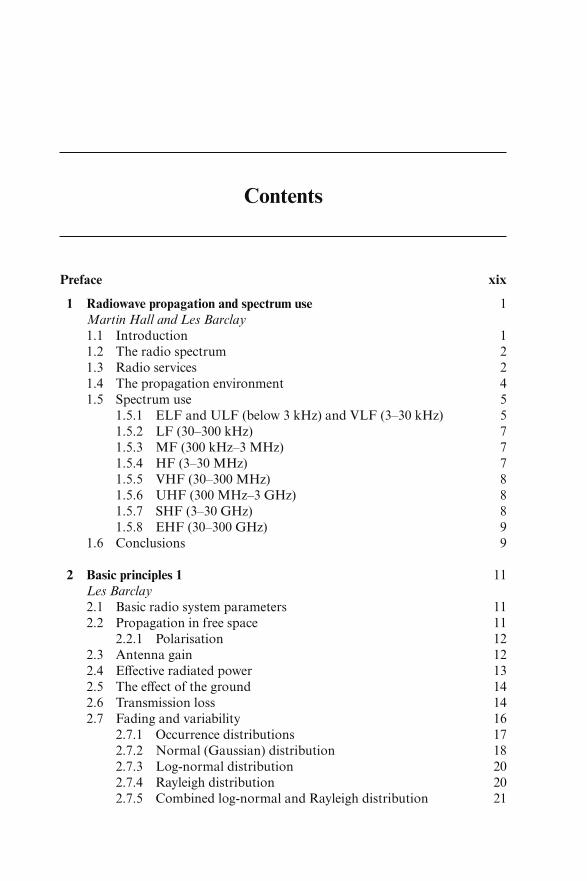
Contents
Preface xix
1 Radiowave propagation and spectrum use 1Martin Hall and Les Barclay
1.1 Introduction 11.2 The radio spectrum 21.3 Radio services 21.4 The propagation environment 41.5 Spectrum use 5
1.5.1 ELF and ULF (below 3 kHz) and VLF (3–30 kHz) 51.5.2 LF (30–300 kHz) 71.5.3 MF (300 kHz–3 MHz) 71.5.4 HF (3–30 MHz) 71.5.5 VHF (30–300 MHz) 81.5.6 UHF (300 MHz–3 GHz) 81.5.7 SHF (3–30 GHz) 81.5.8 EHF (30–300 GHz) 9
1.6 Conclusions 9
2 Basic principles 1 11Les Barclay
2.1 Basic radio system parameters 112.2 Propagation in free space 11
2.2.1 Polarisation 122.3 Antenna gain 122.4 Effective radiated power 132.5 The effect of the ground 142.6 Transmission loss 142.7 Fading and variability 16
2.7.1 Occurrence distributions 172.7.2 Normal (Gaussian) distribution 182.7.3 Log-normal distribution 202.7.4 Rayleigh distribution 202.7.5 Combined log-normal and Rayleigh distribution 21
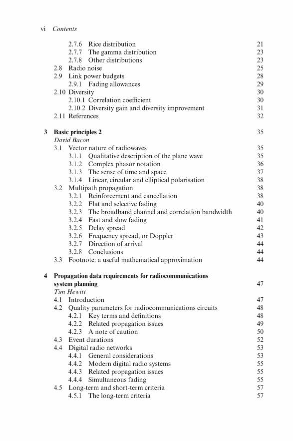
2.7.6 Rice distribution 212.7.7 The gamma distribution 232.7.8 Other distributions 23
2.8 Radio noise 252.9 Link power budgets 28
2.9.1 Fading allowances 292.10 Diversity 30
2.10.1 Correlation coefficient 302.10.2 Diversity gain and diversity improvement 31
2.11 References 32
3 Basic principles 2 35David Bacon
3.1 Vector nature of radiowaves 353.1.1 Qualitative description of the plane wave 353.1.2 Complex phasor notation 363.1.3 The sense of time and space 373.1.4 Linear, circular and elliptical polarisation 38
3.2 Multipath propagation 383.2.1 Reinforcement and cancellation 383.2.2 Flat and selective fading 403.2.3 The broadband channel and correlation bandwidth 403.2.4 Fast and slow fading 413.2.5 Delay spread 423.2.6 Frequency spread, or Doppler 433.2.7 Direction of arrival 443.2.8 Conclusions 44
3.3 Footnote: a useful mathematical approximation 44
4 Propagation data requirements for radiocommunicationssystem planning 47Tim Hewitt
4.1 Introduction 474.2 Quality parameters for radiocommunications circuits 48
4.2.1 Key terms and definitions 484.2.2 Related propagation issues 494.2.3 A note of caution 50
4.3 Event durations 524.4 Digital radio networks 53
4.4.1 General considerations 534.4.2 Modern digital radio systems 554.4.3 Related propagation issues 554.4.4 Simultaneous fading 55
4.5 Long-term and short-term criteria 574.5.1 The long-term criteria 57
vi Contents
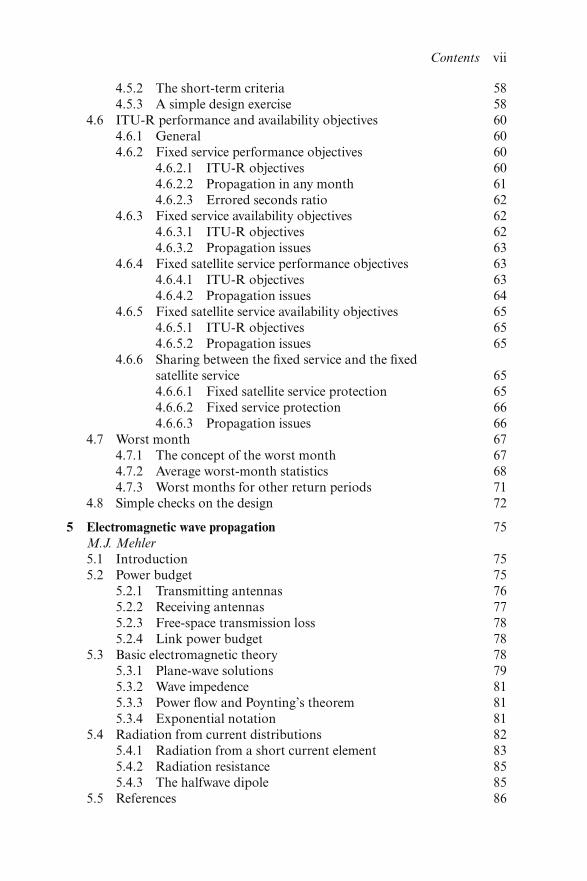
4.5.2 The short-term criteria 584.5.3 A simple design exercise 58
4.6 ITU-R performance and availability objectives 604.6.1 General 604.6.2 Fixed service performance objectives 60
4.6.2.1 ITU-R objectives 604.6.2.2 Propagation in any month 614.6.2.3 Errored seconds ratio 62
4.6.3 Fixed service availability objectives 624.6.3.1 ITU-R objectives 624.6.3.2 Propagation issues 63
4.6.4 Fixed satellite service performance objectives 634.6.4.1 ITU-R objectives 634.6.4.2 Propagation issues 64
4.6.5 Fixed satellite service availability objectives 654.6.5.1 ITU-R objectives 654.6.5.2 Propagation issues 65
4.6.6 Sharing between the fixed service and the fixedsatellite service 654.6.6.1 Fixed satellite service protection 654.6.6.2 Fixed service protection 664.6.6.3 Propagation issues 66
4.7 Worst month 674.7.1 The concept of the worst month 674.7.2 Average worst-month statistics 684.7.3 Worst months for other return periods 71
4.8 Simple checks on the design 72
5 Electromagnetic wave propagation 75M.J. Mehler
5.1 Introduction 755.2 Power budget 75
5.2.1 Transmitting antennas 765.2.2 Receiving antennas 775.2.3 Free-space transmission loss 785.2.4 Link power budget 78
5.3 Basic electromagnetic theory 785.3.1 Plane-wave solutions 795.3.2 Wave impedence 815.3.3 Power flow and Poynting’s theorem 815.3.4 Exponential notation 81
5.4 Radiation from current distributions 825.4.1 Radiation from a short current element 835.4.2 Radiation resistance 855.4.3 The halfwave dipole 85
5.5 References 86
Contents vii
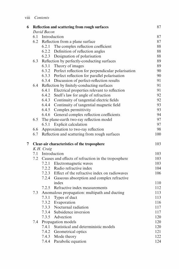
6 Reflection and scattering from rough surfaces 87David Bacon
6.1 Introduction 876.2 Reflection from a plane surface 87
6.2.1 The complex reflection coefficient 886.2.2 Definition of reflection angles 886.2.3 Designation of polarisation 88
6.3 Reflection by perfectly-conducting surfaces 896.3.1 Theory of images 896.3.2 Perfect reflection for perpendicular polarisation 906.3.3 Perfect reflection for parallel polarisation 906.3.4 Discussion of perfect-reflection results 91
6.4 Reflection by finitely-conducting surfaces 916.4.1 Electrical properties relevant to reflection 916.4.2 Snell’s law for angle of refraction 926.4.3 Continuity of tangential electric fields 926.4.4 Continuity of tangential magnetic field 936.4.5 Complex permittivity 936.4.6 General complex reflection coefficients 94
6.5 The plane-earth two-ray reflection model 976.5.1 Explicit calculation 97
6.6 Approximation to two-ray reflection 986.7 Reflection and scattering from rough surfaces 100
7 Clear-air characteristics of the troposphere 103K.H. Craig
7.1 Introduction 1037.2 Causes and effects of refraction in the troposphere 103
7.2.1 Electromagnetic waves 1037.2.2 Radio refractive index 1047.2.3 Effect of the refractive index on radiowaves 1067.2.4 Gaseous absorption and complex refractive
index 1107.2.5 Refractive index measurements 112
7.3 Anomalous propagation: multipath and ducting 1137.3.1 Types of duct 1137.3.2 Evaporation 1167.3.3 Nocturnal radiation 1177.3.4 Subsidence inversion 1177.3.5 Advection 120
7.4 Propagation models 1207.4.1 Statistical and deterministic models 1207.4.2 Geometrical optics 1217.4.3 Mode theory 1227.4.4 Parabolic equation 124
viii Contents
7.5 Turbulent scatter 1247.6 References 127
8 Introduction to diffraction 129David Bacon
8.1 Underlying principles 1298.1.1 Signal variations at the edge of a radio shadow 1298.1.2 Huygens’ construction 1308.1.3 Fresnel knife-edge diffraction and the Cornu Spiral 131
8.2 Mathematical formulation for knife-edge diffraction 1338.3 Application of knife-edge diffraction 136
8.3.1 Diffraction loss 1368.3.2 Fresnel clearance 137
8.4 Ray-based diffraction methods 1388.4.1 GTD/UTD in two dimensions 1398.4.2 A specific UTD formulation 1398.4.3 Sample UTD results 1418.4.4 Diffraction in three dimensions 1428.4.5 Ray-tracing methods 1438.4.6 Further reading 143
8.5 References 143
9 Short-range propagation 145Les Barclay
9.1 Introduction 1459.2 Outdoor propagation 146
9.2.1 Outdoor path categories 1469.2.2 Path loss models 147
9.2.2.1 Line-of-sight within a street canyon 1479.2.2.2 Models for nonline-of-sight situations 149
9.2.3 Influence of vegetation 1529.2.4 Default parameters for site-general calculations 152
9.3 Indoor propagation 1539.3.1 Propagation impairments and measures of quality in
indoor radio systems 1549.3.2 Indoor path loss models 1549.3.3 Delay spread models 156
9.3.3.1 Multipath 1569.3.3.2 RMS delay spread 1569.3.3.3 Effect of polarisation and antenna radiation
pattern 1569.3.3.4 Effect of building materials, furnishings and
furniture 1579.3.3.5 Effect of movement of objects in the room 159
9.4 Propagation in tunnels 160
Contents ix
9.5 Leaky feeder systems 1609.6 The near field 162
10 Numerically intensive propagation prediction methods 163C.C. Constantinou
10.1 Introduction 16310.1.1 Intractability of exact solutions 16310.1.2 General remarks on numerical methods 16410.1.3 Chapter outline 164
10.2 Integral equation methods 16410.2.1 Derivation of integral equation 16510.2.2 Assumptions made in the derivation of the integral
equation 16710.2.3 Numerical evaluation of integral equations 168
10.3 Parabolic equation methods 16910.3.1 Derivation of the parabolic equation 16910.3.2 Summary of assumptions and approximations 17110.3.3 Parabolic equation marching (I) – the split step fast
Fourier transform method 17210.3.4 Parabolic equation marching (II) – finite difference
implementation 17410.3.5 Parabolic equation conclusions 17710.3.6 Sample applications of the parabolic equation method 177
10.4 Ray-tracing methods 17910.4.1 Ray-tracing elements 17910.4.2 Field strength calculation 181
10.5 References 182
11 Outdoor mobile propagation 185Simon R. Saunders
11.1 Introduction 18511.1.1 The outdoor mobile radio channel 18511.1.2 System types 188
11.2 Macrocells 18811.2.1 Introduction 18811.2.2 Definition of parameters 18911.2.3 Empirical path loss models 190
11.2.3.1 Clutter factor models 19111.2.3.2 The Okumura–Hata model 19211.2.3.3 The COST 231–Hata model 19411.2.3.4 Environment categories 194
11.2.4 Physical models 19511.2.4.1 The Ikegami model 19511.2.4.2 Rooftop diffraction 19611.2.4.3 The flat edge model 197
x Contents

11.2.4.4 The Walfisch–Bertoni model 20111.2.4.5 COST231/Walfisch–Ikegami model 202
11.2.5 Computerised planning tools 20311.2.6 Conclusions 203
11.3 Shadowing 20411.3.1 Introduction 20411.3.2 Statistical characterisation 20511.3.3 Impact on coverage 20611.3.4 Location variability 20811.3.5 Correlated shadowing 20911.3.6 Conclusions 210
11.4 Microcells 21111.4.1 Introduction 21111.4.2 Dual-slope empirical models 21111.4.3 Physical models 21311.4.4 Line-of-sight models 213
11.4.4.1 Two-ray models 21311.4.4.2 Street canyon models 214
11.4.5 Nonline-of-sight models 21511.4.5.1 Propagation mechanisms 21511.4.5.2 Site-specific ray models 218
11.4.6 Discussion 21811.4.7 Microcell shadowing 21811.4.8 Conclusions 219
11.5 References 219
12 Propagation in rain and clouds 223J.W.F. Goddard
12.1 Introduction 22312.2 Rain 223
12.2.1 Rain drop size distributions 22312.2.2 Rain drop shapes 226
12.3 Other forms of hydrometeor 22612.3.1 Liquid water clouds and fog 22612.3.2 Ice hydrometeors 22712.3.3 Ice crystals 22712.3.4 Snow 22812.3.5 Hail and graupel 22812.3.6 Melting layer 228
12.4 Refractive indices of ice and water 23012.5 Hydrometeor scattering theory 232
12.5.1 General 23212.5.2 Rayleigh scattering region 23312.5.3 Optical and resonance scattering regions 234
12.6 Attenuation effects 235
Contents xi
12.6.1 Rain and cloud 23512.6.2 Melting layer 237
12.7 Polarisation dependence 23712.7.1 Concept of principal planes 23812.7.2 Differential attenuation and phase shift in rain 23812.7.3 Attenuation – XPD relations 23812.7.4 Rain drop canting angles 24012.7.5 Ice crystal principal planes 24112.7.6 Differential phase shift due to ice 241
12.8 Spatial–temporal structure of rain 24112.8.1 Temporal (rainfall rate) 24112.8.2 Spatial (vertical and horizontal structure) 242
12.9 Bistatic scatter in rain 24312.10 References 245
13 The propagation aspects of broadcasting at VHF and UHF 247J. Middleton
13.1 Introduction 24713.2 Limit of service determination 24813.3 Protection ratios 24913.4 Characteristics of propagation 251
13.4.1 Ground reflections and surface roughness 25113.4.2 Other multipath effects 25213.4.3 Diffraction 25313.4.4 Tropospheric refraction 253
13.5 The measurement of field strength 25413.6 The prediction of field strength 25613.7 Digital broadcasting 258
13.7.1 DAB 25813.7.2 DTT 259
13.8 Appendix 25913.8.1 Field strength measurement and the antenna factor 25913.8.2 The voltage induced in a halfwave dipole 261
14 Propagation aspects of mobile spread spectrum networks 263M.A. Beach and S.A. Allpress
14.1 Introduction to spread spectrum 26314.2 Properties of DS-CDMA waveforms 26414.3 Impact of the mobile channel 26714.4 DS-CDMA system performance 26914.5 DS-CDMA channel measurements and models 27514.6 Support of handover in cellular networks 28014.7 Conclusions 28114.8 Acknowledgements 28314.9 References 283
xii Contents
15 Basic physics of the ionosphere 285H. Rishbeth
15.1 Introduction 28515.1.1 What is the ionosphere? 28515.1.2 Where does the ionosphere fit into the atmosphere? 28515.1.3 When was the ionosphere discovered? 28615.1.4 How do we study the ionosphere? 28715.1.5 Why do we study the ionosphere? 28715.1.6 What are the most important characteristics of the
ionosphere? 28715.2 The environment of the ionosphere 287
15.2.1 Ionising solar radiations 28715.2.2 Temperature at ionospheric heights 28915.2.3 Composition of the upper atmosphere 28915.2.4 The scale height 29015.2.5 The geomagnetic field 291
15.3 Formation and photochemistry of the ionised layers 29215.3.1 The Chapman formula for production of
ionisation 29215.3.2 Chapman layers 29315.3.3 The continuity equation 29415.3.4 Ion chemistry 29415.3.5 The photochemical scheme of the ionosphere 296
15.4 Dynamics of the ionosphere 29715.4.1 Equation of motion of the charged particles 29715.4.2 Motion of charged particles due to winds and electric
fields 29815.4.3 The ionospheric dynamo 29915.4.4 Atmospheric tides 30015.4.5 Atmospheric waves 30015.4.6 Thermospheric winds 30115.4.7 The vertical circulation 30215.4.8 The F2 peak 30215.4.9 The topside ionosphere 303
15.5 Ionospheric phenomena 30315.5.1 The D layer 30315.5.2 The E layer 30415.5.3 Sporadic E 30415.5.4 F layer behaviour 30415.5.5 F2 layer anomalies 30615.5.6 Small-scale irregularities 30715.5.7 The auroral ovals, polar cap and trough 307
15.6 Solar–terrestrial relations and ionospheric storms 30915.6.1 Solar flares and sudden ionospheric
disturbances 309
Contents xiii
15.6.2 Geomagnetic storms 30915.6.3 Ionospheric storms 30915.6.4 Space weather 31015.6.5 Long-term change 310
15.7 Conclusions 31015.8 Bibliography 311
16 Ionospheric propagation 313Paul S. Cannon and Peter A. Bradley
16.1 A systems perspective 31316.2 Ionospheric morphology 31616.3 Theory of propagation in the ionosphere 317
16.3.1 Vertical propagation – no collisions 31716.3.2 Group path and phase path 31816.3.3 Oblique propagation 31816.3.4 Absorption 320
16.4 Ray tracing 32116.4.1 Introduction 32116.4.2 Virtual techniques 321
16.4.2.1 Simple transionospheric models 32216.4.3 Numerical ray tracing 32316.4.4 Analytic ray tracing 323
16.5 The basic MUF, multipath and other HF issues 32316.6 Fading and Doppler effects 32916.7 Modem requirements on SNR, Doppler and
multipath 33016.8 References 333
17 Ionospherice prediction methods and models 335Paul S. Cannon
17.1 Introduction 33517.1.1 System design and service planning 33617.1.2 Short-term adaptation to the propagation
environment 33617.2 Ionospheric models 336
17.2.1 Introduction 33617.2.2 Empirical models 337
17.2.2.1 Electron density profile models 33717.2.2.2 ITU database of ionospheric coefficients 33817.2.2.3 URSI database of ionospheric
coefficients 33917.2.3 Physical ionospheric models 33917.2.4 Parameterised models 339
17.2.4.1 PIM 33917.3 Prediction methods 340
xiv Contents
17.3.1 HF 34017.3.1.1 ICEPAC 340
17.3.2 Computerised models of ionospheric scintillation 34317.4 Application specific models 34617.5 Ionospheric sounders for HF frequency management 34817.6 Real-time updates to models, ionospheric specification and
forecasting 34917.6.1 Introduction 34917.6.2 PRISM 34917.6.3 Ionospheric forecasting 351
17.7 References 352
18 Surface waves, and sky waves below 2 MHz 357John Milsom
18.1 Introduction 35718.2 Applications 35718.3 Surface-wave propagation 358
18.3.1 What is the surface wave? 35818.3.2 Theory for a homogeneous smooth earth 359
18.3.2.1 Plane finitely conducting earth 35918.3.2.2 Spherical finitely conducting earth 362
18.3.3 Atmospheric effects 36318.3.4 ITU-R recommended prediction method 36418.3.5 Ground conductivity maps 36618.3.6 Smooth earth of mixed conductivity 36618.3.7 The effects of buildings 370
18.4 Sky-wave propagation below 2 MHz 37018.4.1 What is the sky wave? – hops and modes 37018.4.2 Waveguide-mode field strength prediction theory 37118.4.3 Wave-hop field strength prediction theory 37318.4.4 An empirical field strength prediction theory 375
18.4.4.1 General features 37618.4.4.2 Terminal losses and sea gain 37618.4.4.3 Polarisation coupling loss 37818.4.4.4 Temporal variability 378
18.5 Antenna efficiency 37918.6 Surface-wave/sky-wave interactions 38118.7 Background noise 38118.8 Acknowledgments 38218.9 References 382
19 Terrestrial line-of-sight links: Recommendations ITU-R P.530 385R.G. Howell
19.1 Introduction 38519.2 Overview of propagation effects 386
Contents xv
19.3 Link design 38619.3.1 General 38619.3.2 Path clearance 387
19.3.2.1 Nondiversity case 38719.3.2.2 Height diversity case 389
19.4 Prediction of system performance 39019.4.1 Propagation in clear air 390
19.4.1.1 Multipath fading on a single hop of a link 39019.4.1.2 Simultaneous clear-air fading on multihop
links 39119.4.1.3 Signal level enhancement 39219.4.1.4 Conversion from average worst month to
average annual distributions 39219.4.1.5 Reduction of system cross-polar
performance due to clear air effects 39219.4.2 Propagation in rain 393
19.4.2.1 Attenuation by rain 39319.4.2.2 Frequency and polarisation scaling of rain
attenuation statistics 39319.4.2.3 Statistics of the number and duration of rain
fades 39419.4.2.4 Rain fading on multihop links 39419.4.2.5 Depolarisation by rain 395
19.5 Mitigation methods 39619.5.1 Techniques without diversity 39619.5.2 Diversity techniques 39619.5.3 Cross-polar cancellation 397
19.6 References 397
20 The principal elements of Recommendation ITU-R P.452 399Tim Hewitt
20.1 Introduction 39920.2 The COST210 approach to developing a new prediction
procedure 39920.3 Radio meteorological studies 40020.4 Propagation measurements 40020.5 The propagation modelling problem 40220.6 Worst month considerations 40320.7 Path profiles 40320.8 Path characterisation 40520.9 The propagation models 405
20.9.1 Line of sight 40620.9.2 Terrain diffraction 40620.9.3 Tropospheric scatter 40720.9.4 Ducting and elevated layer reflection/refraction 409
xvi Contents
20.9.4.1 Factors affecting the reference timepercentage, β per cent 409
20.9.4.2 Land, sea and coastal effects –determining the value of μ1 410
20.9.4.3 Path geometry – setting the value of μ2 41120.9.4.4 Terrain roughness – setting the value of μ3 414
20.9.5 Factors affecting the basic transmission lossreference value, Lbr dB 41520.9.5.1 Free-space loss between the antennas
and their respective horizons 41620.9.5.2 Specific attenuation within the stratified
layer or duct 41620.9.5.3 Coupling at the radio horizons 41620.9.5.4 Close coupling into over-sea ducts 41820.9.5.5 Terrain site shielding 418
20.9.6 Local clutter losses 41920.10 Hydrometeor scatter 421
20.10.1 The COST210 and Recommendation 452 models 42120.10.2 Basic scenario of the Recommendation P.452 version 423
20.11 Deriving the overall prediction 42520.12 References 426
21 Earth–space propagation: Recommendation ITU-R P.618 429R.G. Howell
21.1 Introduction 42921.2 Overview 429
21.2.1 General 42921.2.2 Propagation effects 430
21.3 Ionospheric effects 43121.4 Clear-air effects 431
21.4.1 General 43121.4.2 Free-space loss and attenuation by atmospheric gases 43221.4.3 Phase decorrelation across the antenna aperture 43321.4.4 Beam spreading loss 43321.4.5 Scintillation and multipath fading 43321.4.6 Angle of arrival 43421.4.7 Propagation delays 435
21.5 Hydrometeor effects 43521.5.1 General 43521.5.2 Prediction of attenuation statistics for an average year 436
21.5.2.1 Frequency scaling of rain attenuationstatistics 436
21.5.2.2 Calculation of rain attenuation statisticsfrom rainfall rate statistics 436
21.5.3 Seasonal variations – worst month 437
Contents xvii
21.5.4 Year-to-year variability of rain attenuation statistics 43821.5.5 Fade duration and rate of change 43821.5.6 Short-term variations in the frequency scaling
ratio of attenuations 43921.6 Estimation of total attenuation produced by multiple sources 43921.7 System noise 43921.8 Cross-polarisation effects 441
21.8.1 General 44121.8.2 Calculation of long-term statistics of
hydrometeor-induced cross polarisation 44221.8.3 Joint statistics of XPD and attenuation 44321.8.4 Long-term frequency and polarisation scaling of
statistics of hydrometeor-induced cross polarisation 44321.9 Bandwidth limitations 44421.10 Calculation of long-term statistics for nonGSO paths 44421.11 Mitigation techniques 445
21.11.1 Site diversity 44521.11.2 Transmit power control 44521.11.3 Cross-polarisation cancellation 445
21.12 References 446
Index 449
xviii Contents
Preface
This edition of the book ‘Propagation of Radiowaves’ is an update of theprevious edition and includes descriptions of new findings and of new andimproved propagation models. It is based on the series of lectures given at the8th IEE residential course held at Cambridge in 2000.
The preface to the previous edition noted that the topics of main interest inradio communication continue to change rapidly, with the consequent need fornew questions to be addressed, arising from the planning of new services. Thepressures to provide information for new applications, for improved servicequality and performance, and for more effective use of the radio spectrum,require a wider understanding of radiowave propagation and the developmentof improved prediction methods.
The intention of this book, and of the series of courses on which it is based, isto emphasise propagation engineering, giving sufficient fundamental informa-tion, but going on to describe the use of these principles, together with researchresults, in the formulation of prediction models and planning tools.
The lecture course was designed and organised by a committee comprisingD F Bacon, K H Craig, M T Hewitt and L W Barclay and thanks are due to thiscommittee for arranging a comprehensive and timely programme. Thanks arealso particularly due to the group of expert lecturers who prepared and deliveredthe course material contained in this book.
Study Group 3 of the International Telecommunication Union, Radiocom-munication Sector is devoted to studies of radiowave propagation. The annualmeetings of its working parties aim to include the most recent information intorevisions and updates of its Recommendations for propagation models, etc. Thecourse and this book emphasise the applications of these ITU-R Recommenda-tions, since these provide the most up to date, peer-reviewed information available.
ITU-R Recommendations are available in several series with a prefix letter toindicate the series and a suffix number to indicate the version. Thus Recom-mendation ITU-R P.341–7 refers to the 7th revision of Recommendationnumber 341 in the propagation series. Before using such Recommendations, itwill be desirable to refer to the ITU web site (www.itu.int) (correct at time ofpublication) to check that the version to be used is in fact the latest availablerevision.

Chapter 1
Radiowave propagation and spectrum use
Martin Hall and Les Barclay
1.1 Introduction
When Heinrich Hertz undertook his experiments to verify that radiowaves wereelectromagnetic radiation which behaved as expected from the theory developedby Maxwell, he probably used frequencies between 50 and 500 MHz. He selectedthe frequency by adjusting the size of the radiating structure, and chose it so thathe could observe the propagation effects of reflection and refraction within hislaboratory. The first public demonstration of a communication system by OliverLodge also probably used a frequency in the VHF range and signals werepropagated about 60 m into the lecture hall. Marconi and others took up thisidea, and Marconi in particular, by increasing the size of the antennas, reducedthe frequency and was able to exploit the better long-distance propagationproperties at progressively lower frequencies.
From the beginning it has been the practical use of the propagation of elec-tromagnetic waves over long distances, together with the ability to modulate thewaves and thus transfer information, which has provided the opportunity forthe development of radio and electronic technologies. This in turn has driven aneed to extend knowledge of the propagation environment, and to characterisethe transfer function of the radio channel to provide greater communicationbandwidths and greater quality of service.
Propagation in free space, or in a uniform dielectric medium, may bedescribed simply. It is the effect of the earth and its surrounding environmentwhich leads to variability and distortion of the radio signal, and which providesthe challenge for the propagation engineer. He seeks to provide a detaileddescription of the signal and a prediction capability for use in the design,planning and operation of radio systems.
1.2 The radio spectrum
Electromagnetic waves may exist with an extremely wide range of wavelengths,and with corresponding frequencies, where the product of frequency andwavelength is the velocity of propagation. In vacuum or air this is very close to3 × 108 m s−1.
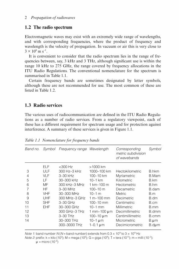
It is convenient to consider that the radio spectrum lies in the range of fre-quencies between, say, 3 kHz and 3 THz, although significant use is within therange 10 kHz to 275 GHz, the range covered by frequency allocations in theITU Radio Regulations. The conventional nomenclature for the spectrum issummarised in Table 1.1.
Certain frequency bands are sometimes designated by letter symbols,although these are not recommended for use. The most common of these arelisted in Table 1.2.
1.3 Radio services
The various uses of radiocommunication are defined in the ITU Radio Regula-tions as a number of radio services. From a regulatory viewpoint, each ofthese has a different requirement for spectrum usage and for protection againstinterference. A summary of these services is given in Figure 1.1.
Table 1.1 Nomenclature for frequency bands
Band no. Symbol Frequency range Wavelength Correspondingmetric subdivisionof wavebands
Symbol
ELF <300 Hz >1000 km3 ULF 300 Hz–3 kHz 1000–100 km Hectokilometric B.hkm4 VLF 3–30 kHz 100–10 km Myriametric B.Mam5 LF 30–300 kHz 10–1 km Kilometric B.km6 MF 300 kHz–3 MHz 1 km–100 m Hectometric B.hm7 HF 3–30 MHz 100–10 m Decametric B.dam8 VHF 30–300 MHz 10–1 m Metric B.m9 UHF 300 MHz–3 GHz 1 m–100 mm Decimetric B.dm
10 SHF 3–30 GHz 100–10 mm Centimetric B.cm11 EHF 30–300 GHz 10–1 mm Millimetric B.mm12 300 GHz–3 THz 1 mm–100 �m Decimillimetric B.dmm13 3–30 THz 100–10 �m Centimillimetric B.cmm14 30–300 THz 10–1 �m Micrometric B.�m
300–3000 THz 1–0.1 �m Decimicrometric B.d�m
Note 1: band number N (N = band number) extends from 0.3 × 10N to 3 × 10N HzNote 2: prefix: k = kilo (103); M = mega (106); G = giga (109); T = tera (1012); m = milli (10−3);
� = micro (10−6)
2 Propagation of radiowaves
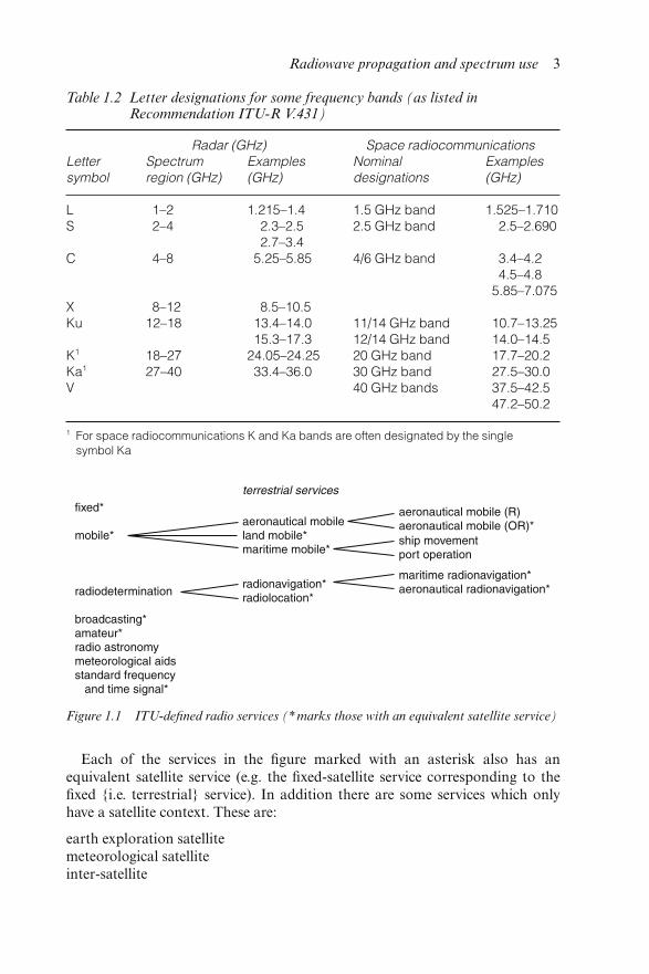
Each of the services in the figure marked with an asterisk also has anequivalent satellite service (e.g. the fixed-satellite service corresponding to thefixed {i.e. terrestrial} service). In addition there are some services which onlyhave a satellite context. These are:
earth exploration satellitemeteorological satelliteinter-satellite
Figure 1.1 ITU-defined radio services (*marks those with an equivalent satellite service)
Table 1.2 Letter designations for some frequency bands (as listed inRecommendation ITU-R V.431)
Radar (GHz) Space radiocommunicationsLettersymbol
Spectrumregion (GHz)
Examples(GHz)
Nominaldesignations
Examples(GHz)
L 1–2 1.215–1.4 1.5 GHz band 1.525–1.710S 2–4 2.3–2.5
2.7–3.42.5 GHz band 2.5–2.690
C 4–8 5.25–5.85 4/6 GHz band 3.4–4.24.5–4.8
5.85–7.075X 8–12 8.5–10.5Ku 12–18 13.4–14.0
15.3–17.311/14 GHz band12/14 GHz band
10.7–13.2514.0–14.5
K1 18–27 24.05–24.25 20 GHz band 17.7–20.2Ka1 27–40 33.4–36.0 30 GHz band 27.5–30.0V 40 GHz bands 37.5–42.5
47.2–50.2
1 For space radiocommunications K and Ka bands are often designated by the singlesymbol Ka
Radiowave propagation and spectrum use 3
space operationsspace research
Recent developments in the use of radio for a variety of applications means thatthis division into services may become increasingly less appropriate. It may bebetter to distinguish uses by the precision in the identification of the location ofthe radio link terminals, by the ability to exploit directional antennas, bythe height of the antennas in relation to the surrounding buildings or groundfeatures, or by the required bandwidth etc.
1.4 The propagation environment
Except for the inter-satellite service, where the propagation path may be entirelyin near free-space conditions, propagation for all radio applications may beaffected by the earth and its surrounding atmosphere.
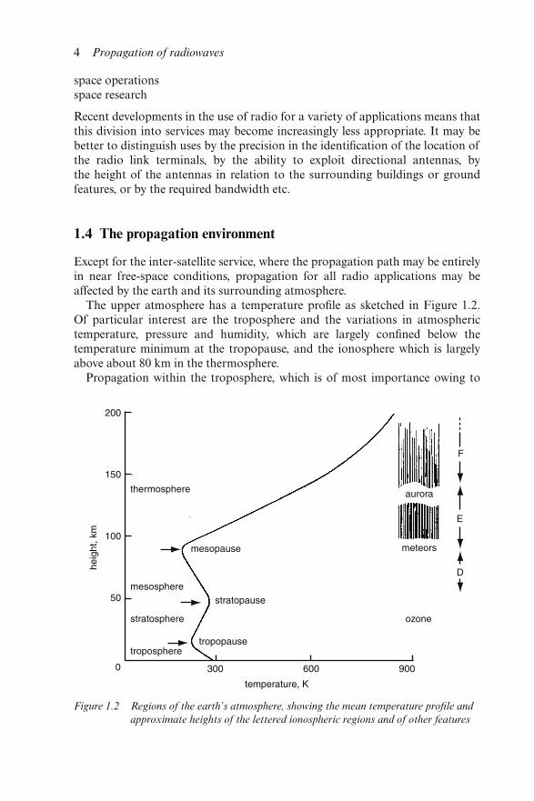
The upper atmosphere has a temperature profile as sketched in Figure 1.2.Of particular interest are the troposphere and the variations in atmospherictemperature, pressure and humidity, which are largely confined below thetemperature minimum at the tropopause, and the ionosphere which is largelyabove about 80 km in the thermosphere.
Propagation within the troposphere, which is of most importance owing to
Figure 1.2 Regions of the earth’s atmosphere, showing the mean temperature profile and
approximate heights of the lettered ionospheric regions and of other features
4 Propagation of radiowaves
the wide variety of uses and the very wide available bandwidths at higher fre-quencies, is complex due to irregularities in the refractive index profile and to thepresence of rain and other hydrometeors. The effects are summarised diagram-matically in Figure 1.3.
The profile of electron density in the ionosphere acts as a reflecting layercapable of reflecting signals at HF and lower frequencies back to earth. Thereare occasional effects which permit some reflection or scatter back to earth atVHF. The ionosphere also has some important effects on earth–space paths upto SHF.
In addition, diffraction, reflection and scatter in relation to the ground andboth man-made and natural structures on the surface are of great importance.
All of these aspects will be addressed in subsequent chapters.
1.5 Spectrum use
It is useful to review the way in which each part of the spectrum is used.Although the conventional way of describing the spectrum in decade frequencybands does not match the applications or the propagation characteristicsvery well, it is used here as a convenient shorthand. None of the frequencyboundaries indicated is clear and precise in terms of differing usage.
1.5.1 ELF and ULF (below 3 kHz) and VLF (3–30 kHz)
Typical services: worldwide telegraphy to ships and submarines;worldwide communication, mine and subterraneancommunication;
System considerations: even the largest antennas have a size which is only asmall fraction of a wavelength, resulting in lowradiation resistance; it is difficult to make transmitterantennas directional; bandwidth is very limited,resulting in only low or very low data rates; there is highatmospheric noise so that inefficient receiving antennasare satisfactory
Propagation: in earth–ionosphere waveguide, with relatively stablepropagation; affected by thick ice masses (e.g.Greenland); propagation east/west and west/east isasymmetric; useful propagation through sea water,which has significant skin depth at these wavelengths
Comment: there are no international frequency allocations below9 kHz; there is limited use of frequencies below 9 kHzfor military purposes; the successful Omega worldwidenavigation system has recently been closed
Radiowave propagation and spectrum use 5
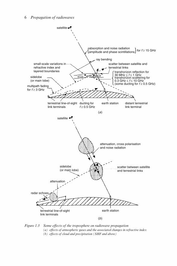
Figure 1.3 Some effects of the troposphere on radiowave propagation(a) effects of atmospheric gases and the associated changes in refractive index
(b) effects of cloud and precipitation (SHF and above)
6 Propagation of radiowaves
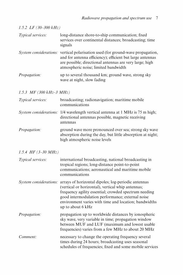
1.5.2 LF (30–300 kHz)
Typical services: long-distance shore-to-ship communication; fixedservices over continental distances; broadcasting; timesignals
System considerations: vertical polarisation used (for ground-wave propagation,and for antenna efficiency); efficient but large antennasare possible; directional antennas are very large; highatmospheric noise; limited bandwidth
Propagation: up to several thousand km; ground wave, strong skywave at night, slow fading
1.5.3 MF (300 kHz–3 MHz)
Typical services: broadcasting; radionavigation; maritime mobilecommunications
System considerations: 1/4 wavelength vertical antenna at 1 MHz is 75 m high;directional antennas possible, magnetic receivingantennas
Propagation: ground wave more pronounced over sea; strong sky waveabsorption during the day, but little absorption at night;high atmospheric noise levels
1.5.4 HF (3–30 MHz)
Typical services: international broadcasting, national broadcasting intropical regions; long-distance point-to-pointcommunications; aeronautical and maritime mobilecommunications
System considerations: arrays of horizontal dipoles; log-periodic antennas(vertical or horizontal), vertical whip antennas;frequency agility essential; crowded spectrum needinggood intermodulation performance; external noiseenvironment varies with time and location; bandwidthsup to about 6 kHz
Propagation: propagation up to worldwide distances by ionosphericsky wave, very variable in time; propagation windowbetween MUF and LUF (maximum and lowest usablefrequencies) varies from a few MHz to about 20 MHz
Comment: necessary to change the operating frequency severaltimes during 24 hours; broadcasting uses seasonalschedules of frequencies; fixed and some mobile services
Radiowave propagation and spectrum use 7
use intelligent frequency adaptive systems; continues toprovide the main intercontinental air traffic controlsystem; most modulation bandwidths may exceed thecorrelation bandwidth
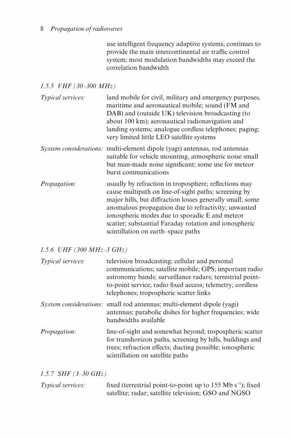
1.5.5 VHF (30–300 MHz)
Typical services: land mobile for civil, military and emergency purposes,maritime and aeronautical mobile; sound (FM andDAB) and (outside UK) television broadcasting (toabout 100 km); aeronautical radionavigation andlanding systems; analogue cordless telephones; paging;very limited little LEO satellite systems
System considerations: multi-element dipole (yagi) antennas, rod antennassuitable for vehicle mounting, atmospheric noise smallbut man-made noise significant; some use for meteorburst communications
Propagation: usually by refraction in troposphere; reflections maycause multipath on line-of-sight paths; screening bymajor hills, but diffraction losses generally small; someanomalous propagation due to refractivity; unwantedionospheric modes due to sporadic E and meteorscatter; substantial Faraday rotation and ionosphericscintillation on earth–space paths
1.5.6 UHF (300 MHz–3 GHz)
Typical services: television broadcasting; cellular and personalcommunications; satellite mobile; GPS; important radioastronomy bands; surveillance radars; terrestrial point-to-point service; radio fixed access; telemetry; cordlesstelephones; tropospheric scatter links
System considerations: small rod antennas; multi-element dipole (yagi)antennas; parabolic dishes for higher frequencies; widebandwidths available
Propagation: line-of-sight and somewhat beyond; tropospheric scatterfor transhorizon paths, screening by hills, buildings andtrees; refraction effects; ducting possible; ionosphericscintillation on satellite paths
1.5.7 SHF (3–30 GHz)
Typical services: fixed (terrestrial point-to-point up to 155 Mb s−1); fixedsatellite; radar; satellite television; GSO and NGSO
8 Propagation of radiowaves
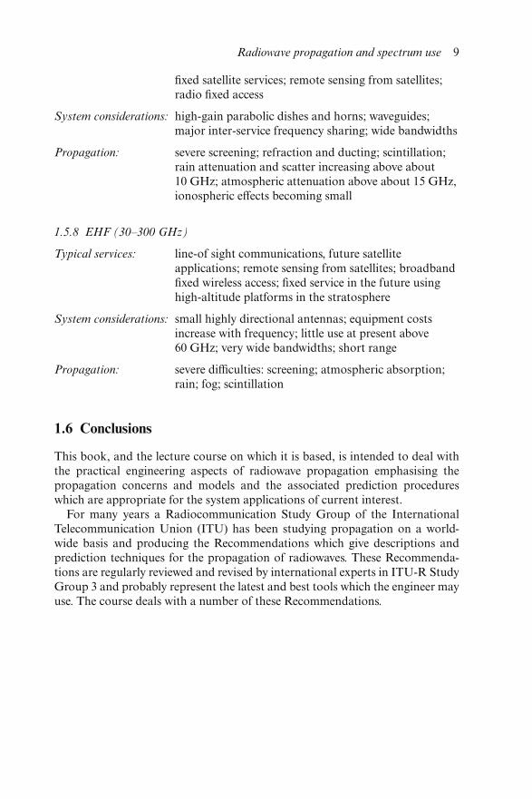
fixed satellite services; remote sensing from satellites;radio fixed access
System considerations: high-gain parabolic dishes and horns; waveguides;major inter-service frequency sharing; wide bandwidths
Propagation: severe screening; refraction and ducting; scintillation;rain attenuation and scatter increasing above about10 GHz; atmospheric attenuation above about 15 GHz,ionospheric effects becoming small
1.5.8 EHF (30–300 GHz)
Typical services: line-of sight communications, future satelliteapplications; remote sensing from satellites; broadbandfixed wireless access; fixed service in the future usinghigh-altitude platforms in the stratosphere
System considerations: small highly directional antennas; equipment costsincrease with frequency; little use at present above60 GHz; very wide bandwidths; short range
Propagation: severe difficulties: screening; atmospheric absorption;rain; fog; scintillation
1.6 Conclusions
This book, and the lecture course on which it is based, is intended to deal withthe practical engineering aspects of radiowave propagation emphasising thepropagation concerns and models and the associated prediction procedureswhich are appropriate for the system applications of current interest.
For many years a Radiocommunication Study Group of the InternationalTelecommunication Union (ITU) has been studying propagation on a world-wide basis and producing the Recommendations which give descriptions andprediction techniques for the propagation of radiowaves. These Recommenda-tions are regularly reviewed and revised by international experts in ITU-R StudyGroup 3 and probably represent the latest and best tools which the engineer mayuse. The course deals with a number of these Recommendations.
Radiowave propagation and spectrum use 9

Chapter 2
Basic principles 1
Les Barclay
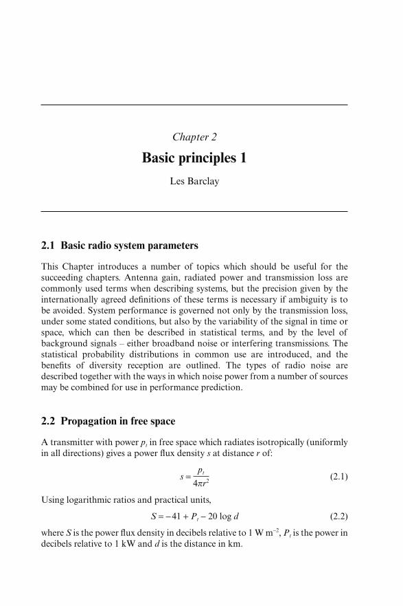
2.1 Basic radio system parameters
This Chapter introduces a number of topics which should be useful for thesucceeding chapters. Antenna gain, radiated power and transmission loss arecommonly used terms when describing systems, but the precision given by theinternationally agreed definitions of these terms is necessary if ambiguity is tobe avoided. System performance is governed not only by the transmission loss,under some stated conditions, but also by the variability of the signal in time orspace, which can then be described in statistical terms, and by the level ofbackground signals – either broadband noise or interfering transmissions. Thestatistical probability distributions in common use are introduced, and thebenefits of diversity reception are outlined. The types of radio noise aredescribed together with the ways in which noise power from a number of sourcesmay be combined for use in performance prediction.
2.2 Propagation in free space
A transmitter with power pt in free space which radiates isotropically (uniformlyin all directions) gives a power flux density s at distance r of:
s = pt
4πr2(2.1)
Using logarithmic ratios and practical units,
S = −41 + Pt − 20 log d (2.2)
where S is the power flux density in decibels relative to 1 W m−2, Pt is the power indecibels relative to 1 kW and d is the distance in km.
The corresponding field strength e is given by:
e = √120πs = √30pt
r(2.3)
This relationship applies when the power is radiated isotropically.A λ/2 dipole has a gain in its equatorial plane of 1.64 times (see below) and in
this case the field strength is:
e ≈ 7√pt
r(2.4)
From the above, for free-space propagation, the signal intensity, or the fieldstrength, decreases by 20 dB for each decade of increasing distance, or by 6 dBfor each doubling of distance.
2.2.1 Polarisation
The concept of wave polarisation will be discussed further in Chapters 5 and 6.Suffice it to say here that an electromagnetic wave will have a characteristicpolarisation, usually described by the plane of the electric field. For linearantennas in free space the polarisation plane will correspond to the plane con-taining the electric radiating element of the antenna. For the above expressionsfor signal intensity it is assumed that the receiving antenna is also oriented in theplane of polarisation.
2.3 Antenna gain
The ITU Radio Regulations formally define the gain of an antenna as: ‘Theratio, usually expressed in decibels, of the power required at the input of a loss-free reference antenna to the power supplied to the input of the given antenna toproduce, in a given direction, the same field strength or the same power fluxdensity at the same distance’. When not specified otherwise, the gain refers to thedirection of maximum radiation. The gain may be considered for a specifiedpolarisation. Gain greater than unity (positive in terms of decibels) will increasethe power radiated in a given direction and corresponds to an increase in theeffective aperture of a receiving antenna.
Depending on the choice of the reference antenna, a distinction is madebetween:
(a) absolute or isotropic gain (Gi), when the reference antenna is an isotropicantenna isolated in space (note that isotropic radiation relates to an equalintensity in all directions; the term omnidirectional radiation is often usedfor an antenna which radiates equally at all azimuths in the horizontalplane, such an antenna may radiate with a different intensity for otherelevation angles);
12 Propagation of radiowaves
(b) gain relative to a halfwave dipole (Gd), when the reference antenna is ahalfwave dipole isolated in space whose equatorial plane contains the givendirection;
(c) gain relative to a short vertical antenna conductor (Gv) much shorter thanone-quarter of the wavelength, on and normal to the surface of a perfectlyconducting plane which contains the given direction.
An isotropic radiator is often adopted as the reference at microwaves and at HF,and a halfwave dipole is often adopted at VHF and UHF, where this type ofantenna is convenient for practical implementation. A short vertical antennaover a conducting ground is an appropriate reference at MF and lower frequen-cies where ground-wave propagation is involved and this usage extends tosky-wave propagation at MF and, in older texts, at HF.
The comparative gains of these reference antennas, and of some otherantenna types, are given in Table 2.1.
2.4 Effective radiated power
The Radio Regulations also provide definitions for effective or equivalentradiated power, again in relation to the three reference antennas:
(i) equivalent isotropically radiated power (EIRP): the product of the powersupplied to the antenna and the antenna gain in a given direction relativeto an isotropic antenna (absolute or isotropic gain); specification of anEIRP in decibels may be made using the symbol dBi;
(ii) effective radiated power (ERP): the product of the power supp1ied to theantenna and its gain in a given direction relative to a halfwave dipole;
(iii) effective monopole radiated power (EMRP): the product of the power
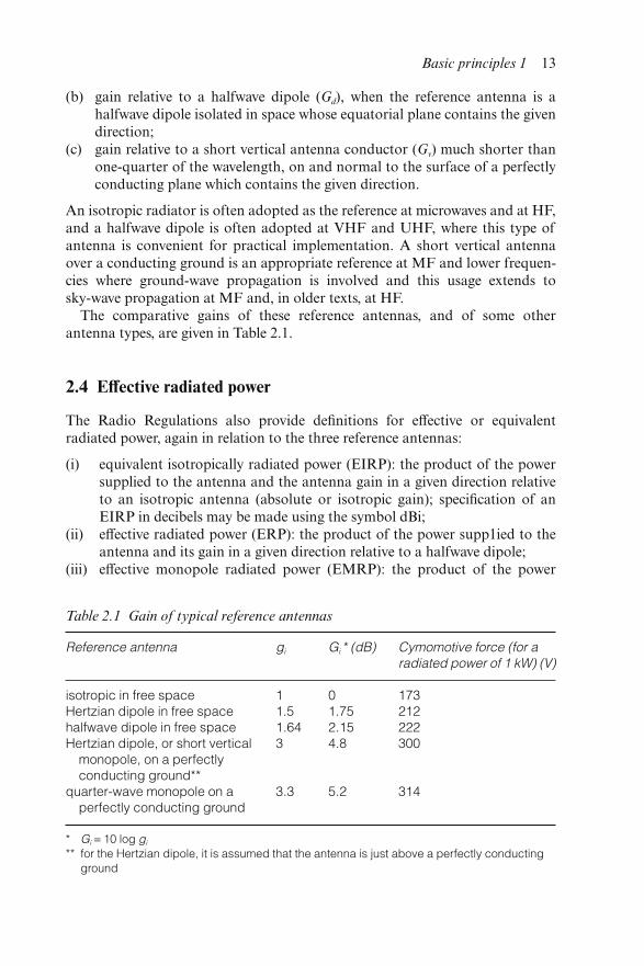
Table 2.1 Gain of typical reference antennas
Reference antenna gi Gi * (dB) Cymomotive force (for aradiated power of 1 kW) (V)
isotropic in free space 1 0 173Hertzian dipole in free space 1.5 1.75 212halfwave dipole in free space 1.64 2.15 222Hertzian dipole, or short vertical
monopole, on a perfectlyconducting ground**
3 4.8 300
quarter-wave monopole on aperfectly conducting ground
3.3 5.2 314
* Gi = 10 log gi
** for the Hertzian dipole, it is assumed that the antenna is just above a perfectly conductingground
Basic principles 1 13
supplied to the antenna and its gain in a given direction relative to a shortvertical antenna.
Note that ERP, which is often used as a general term for radiated power, strictlyonly applies when the reference antenna is a halfwave dipole.
An alternative way of indicating the intensity of radiation, which is some-times used at the lower frequencies, is in terms of the cymomotive force,expressed in volts. The cymomotive force is given by the product of the fieldstrength and the distance, assuming loss-free radiation. Values of cymomotiveforce when 1 kW is radiated from the reference antennas are also given inTable 2.1.
2.5 The effect of the ground
The proximity of the imperfectly conducting ground will affect the performanceof an antenna. In some cases, where the antenna is located several wavelengthsabove the ground, it may be convenient to consider signals directly from (or to)the antenna and those which are reflected from the ground or another nearbysurface as separate signal ray paths. When the antenna is close to, or on, theground it is no longer appropriate to consider separate rays and then the effectmay be taken into account by assuming a modified directivity pattern for theantenna, including the ground reflection; by modifying the effective aperture ofthe antenna; or by taking account of the change in radiation resistance etc. Adiscussion of this for the ground-wave case, where the problem is most difficult,is contained in Annex II of Recommendation ITU-R P.341.
Information concerning the electrical characteristics of the surface of theearth is contained in further ITU-R texts: Recommendations ITU-R P.527and P.832.
2.6 Transmission loss
The power available, pr, in a load which is conjugately matched to the impedanceof a receiving antenna is:
pr = sae (2.5)
where ae is the effective aperture of the antenna, given by λ2/4π for an idealloss-free isotropic antenna.
Thus from Eqn. 2.1 the power received by an ideal isotropic antenna atdistance r due to power pt radiated isotropically is given by:
pr = pt
4πr2 = pt� λ
4πr�2
(2.6)
and the free-space basic transmission loss is the ratio pt/pr.
14 Propagation of radiowaves
Transmission losses are almost always expressed in logarithmic terms, indecibels, and as a positive value of attenuation, i.e.
Lbf = 10 log �pt
pr� = Pt − Pr = 20 log �4πr
λ � (2.7)
or
Lbf = 32.44 + 20 log f + 20 log d (2.8)
where f is in MHz and d is in km.The concept of transmission loss may be extended to include the effects of the
following mechanisms in the propagation medium, and of the antennas and theradio system actually in use:
Free-space basic transmission loss Lbf relates to isotropic antennas and loss-freepropagation;
Basic transmission loss Lb includes the effect of the propagation medium, e.g.
(a) absorption loss due to atmospheric gases or in the ionosphere(b) diffraction loss due to obstructions such as hills or buildings(c) reflection losses, including focusing or defocusing due to curvature of
reflecting layers(d) scattering due to irregularities in the atmospheric refractive index or in the
ionosphere or by hydrometeors(e) aperture-to-medium coupling loss or antenna gain degradation, which may
be due to the presence of substantial scatter phenomena on the path(f) polarisation coupling loss; this can arise from any polarisation mismatch
between the antennas for the particular ray path considered(g) effect of wave interference between the direct ray and rays reflected from the
ground, other obstacles or atmospheric layers
Transmission loss L includes the directivity of the actual transmitting antennas,disregarding antenna circuit losses;
System loss Ls is obtained from the powers at the antenna terminals;
Total loss Lt is the ratio determined at convenient, specified, points within thetransmitter and receiver systems.
The relationships between these loss ratios are illustrated in Figure 2.1. It isimportant to be precise when using the terms, and the full definitions are given inRecommendation ITU-R P.341.
Basic principles 1 15
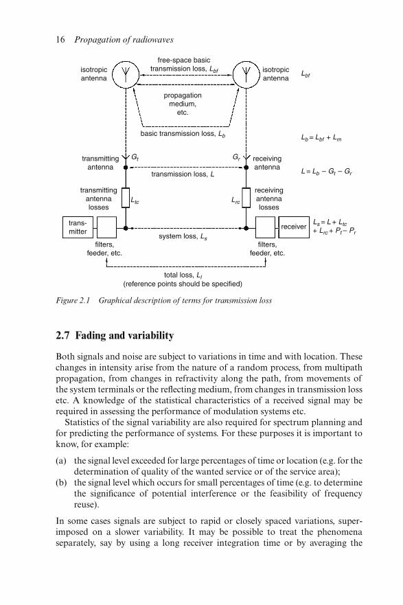
2.7 Fading and variability
Both signals and noise are subject to variations in time and with location. Thesechanges in intensity arise from the nature of a random process, from multipathpropagation, from changes in refractivity along the path, from movements ofthe system terminals or the reflecting medium, from changes in transmission lossetc. A knowledge of the statistical characteristics of a received signal may berequired in assessing the performance of modulation systems etc.
Statistics of the signal variability are also required for spectrum planning andfor predicting the performance of systems. For these purposes it is important toknow, for example:
(a) the signal level exceeded for large percentages of time or location (e.g. for thedetermination of quality of the wanted service or of the service area);
(b) the signal level which occurs for small percentages of time (e.g. to determinethe significance of potential interference or the feasibility of frequencyreuse).
In some cases signals are subject to rapid or closely spaced variations, super-imposed on a slower variability. It may be possible to treat the phenomenaseparately, say by using a long receiver integration time or by averaging the
Figure 2.1 Graphical description of terms for transmission loss
16 Propagation of radiowaves
level of the signal (e.g. with AGC) so that the time interval adopted encom-passes many individual short-term or closely spaced fluctuations. In othercases an understanding of the overall variability of the signal may require aconsideration of the combined effects of two types of variability.
2.7.1 Occurrence distributions
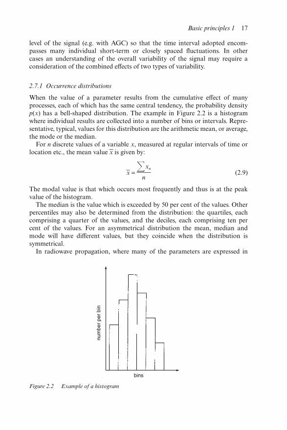
When the value of a parameter results from the cumulative effect of manyprocesses, each of which has the same central tendency, the probability densityp(x) has a bell-shaped distribution. The example in Figure 2.2 is a histogramwhere individual results are collected into a number of bins or intervals. Repre-sentative, typical, values for this distribution are the arithmetic mean, or average,the mode or the median.
For n discrete values of a variable x, measured at regular intervals of time orlocation etc., the mean value x is given by:
x = �xn
n(2.9)
The modal value is that which occurs most frequently and thus is at the peakvalue of the histogram.
The median is the value which is exceeded by 50 per cent of the values. Otherpercentiles may also be determined from the distribution: the quartiles, eachcomprising a quarter of the values, and the deciles, each comprising ten percent of the values. For an asymmetrical distribution the mean, median andmode will have different values, but they coincide when the distribution issymmetrical.
In radiowave propagation, where many of the parameters are expressed in
Figure 2.2 Example of a histogram
Basic principles 1 17
decibels, an arithmetic mean of a set of logarithmic values in decibels makeslittle sense, and the median and other percentiles are much more useful.
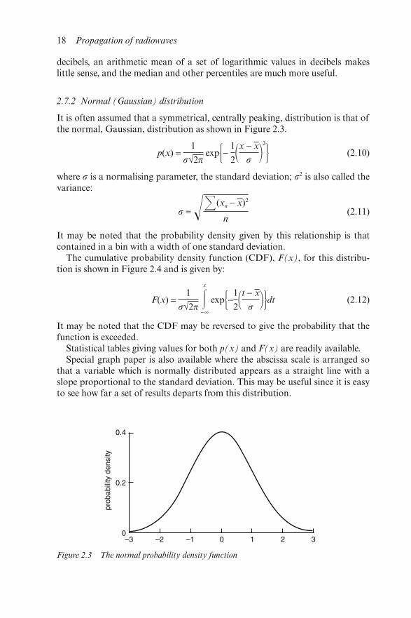
2.7.2 Normal (Gaussian) distribution
It is often assumed that a symmetrical, centrally peaking, distribution is that ofthe normal, Gaussian, distribution as shown in Figure 2.3.
p(x) = 1
σ√2π exp�− 1
2�x − x
σ �2
� (2.10)
where σ is a normalising parameter, the standard deviation; σ2 is also called thevariance:
σ = ��(xn − x)2
n(2.11)
It may be noted that the probability density given by this relationship is thatcontained in a bin with a width of one standard deviation.
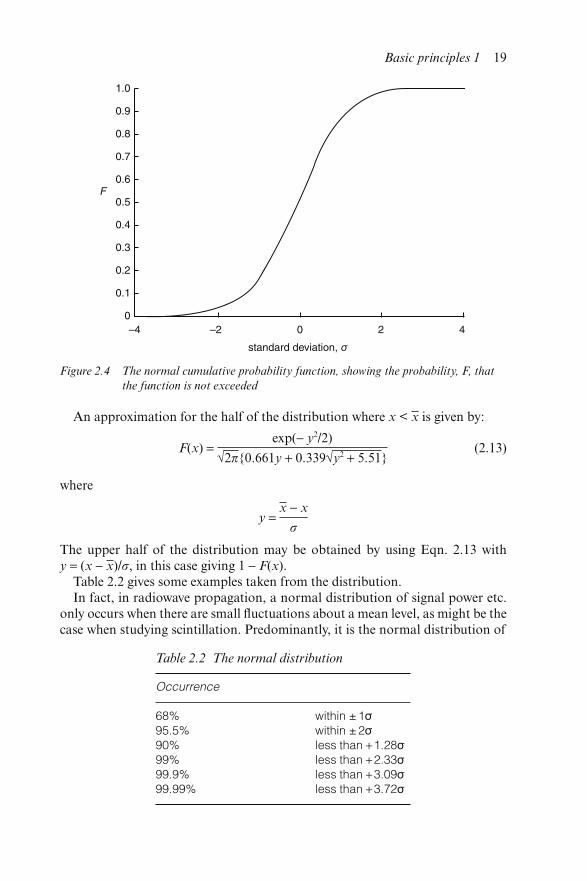
The cumulative probability density function (CDF), F(x), for this distribu-tion is shown in Figure 2.4 and is given by:
F(x) =1
σ√2π�x
−∞
exp�−1
2�t − x
σ ��dt (2.12)
It may be noted that the CDF may be reversed to give the probability that thefunction is exceeded.
Statistical tables giving values for both p(x) and F(x) are readily available.Special graph paper is also available where the abscissa scale is arranged so
that a variable which is normally distributed appears as a straight line with aslope proportional to the standard deviation. This may be useful since it is easyto see how far a set of results departs from this distribution.
Figure 2.3 The normal probability density function
18 Propagation of radiowaves
An approximation for the half of the distribution where x < x is given by:
F(x) =exp(− y2/2)
√2π{0.661y + 0.339√y2 + 5.51}(2.13)
where
y = x − x
σ
The upper half of the distribution may be obtained by using Eqn. 2.13 withy = (x − x)/σ, in this case giving 1 − F(x).
Table 2.2 gives some examples taken from the distribution.In fact, in radiowave propagation, a normal distribution of signal power etc.
only occurs when there are small fluctuations about a mean level, as might be thecase when studying scintillation. Predominantly, it is the normal distribution of
Figure 2.4 The normal cumulative probability function, showing the probability, F, that
the function is not exceeded
Table 2.2 The normal distribution
Occurrence
68% within ±1�95.5% within ±2�90% less than +1.28�99% less than +2.33�99.9% less than +3.09�99.99% less than +3.72�
Basic principles 1 19
the logarithms of the variable which gives useful information: the log-normaldistribution.
2.7.3 Log-normal distribution
In the case of a log-normal distribution, each parameter (the values of thevariable itself, the mean, the standard deviation etc.) is expressed in decibels andthe equations in Section 2.7.2 then apply. The log-normal distribution isappropriate for very many of the time series encountered in propagation studies,and in some cases also for the variations with location, for example within asmall area of the coverage of a mobile system. Note that, when a function is log-normally distributed, the mean and median of the function itself (for exampleexpressed in watts or volts) are not the same: the median is still defined as thecentral value of the distribution, whereas the mean of the numerical values uponwhich the log-normal distribution is based is given by x + σ2/2.
2.7.4 Rayleigh distribution
The combination of a large number (at least more than three) of componentsignal vectors with arbitrary phase and similar amplitude leads to the Rayleighdistribution. Thus, this is appropriate for situations where the signal results fromthe combination of multipath or scatter components. In this case
p(x) = 2x
bexp�− x2
b2� (2.14)
and
F(x) = 1 − exp�− x2
b2� (2.15)
where b is the root mean square value (note that x and b are numerical amplitudevalues, not decibels).
For this distribution the mean is 0.886b, the median is 0.833b, the mode is0.707b and the standard deviation is 0.463b.
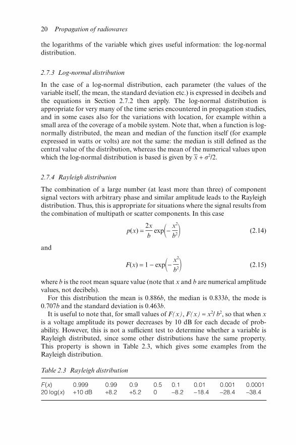
It is useful to note that, for small values of F(x), F(x) ≈ x2/ b2, so that when xis a voltage amplitude its power decreases by 10 dB for each decade of prob-ability. However, this is not a sufficient test to determine whether a variable isRayleigh distributed, since some other distributions have the same property.This property is shown in Table 2.3, which gives some examples from theRayleigh distribution.
Table 2.3 Rayleigh distribution
F (x) 0.999 0.99 0.9 0.5 0.1 0.01 0.001 0.000120 log(x) +10 dB +8.2 +5.2 0 −8.2 −18.4 −28.4 −38.4
20 Propagation of radiowaves
Special graph paper is also available on which a Rayleigh distribution is plot-ted as a straight line: this is the presentation used in Figure 2.6 where the linemarked −∞ dB is a Rayleigh distribution. Note, however, that such a presentationgreatly overemphasises the appearance of small time percentages, and careshould be taken that this does not mislead in the interpretation of plotted results.
2.7.5 Combined log-normal and Rayleigh distribution
In a number of cases the variation of the signal may be represented as havingtwo components: rapid or closely spaced fluctuations, which may be due tomultipath or scatter, with a Rayleigh distribution; and the mean of these rapidvariations, measured over a longer period of time or a longer distance, with alog-normal distribution.
This distribution is given by Boithias [1]:
1 − F(x) = 1
√2π �
∞
−∞
exp�− x2 exp{−0.23σu}u2
2 �du (2.16)
where σ is the standard deviation (in decibels) of the log-normal distribution.This combined distribution is shown in Figure 2.5. This combination of distri-butions has also been studied by Suzuki, and his proposed formulation has beenevaluated by Lorenz [2].
2.7.6 Rice distribution
The Rice distribution (also called the Nakagami-n distribution) applies to thecase where there is a steady, nonfading, component together with a randomvariable component with a Rayleigh distribution. This may occur where there isa direct signal together with a signal reflected from a rough surface, where thereis a steady signal together with multipath signals, or at LF and MF where thereis a steady ground-wave signal and a signal reflected from the ionosphere.
The probability density for the Rice distribution is given by
p(r) = 2r
b2exp�− r2 + a2
b2 �⋅I0�ax
σ2� (2.17)
and
1 − F(x) = 2exp(−a2/b2) �∞
x/b
v exp(−ν2)⋅I0�2aν
b �dν (2.18)
where
I0(z) = 1
π �
π
0
e−z cosθdθ (2.19)
Basic principles 1 21
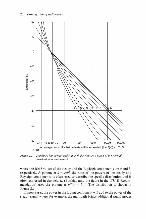
where the RMS values of the steady and the Rayleigh components are a and b,respectively. A parameter k = a2/b2, the ratio of the powers of the steady andRayleigh components, is often used to describe the specific distribution and isoften expressed in decibels, K. (Boithias (and the figure in the ITU-R Recom-mendation) uses the parameter b2/(a2 + b2).) The distribution is shown inFigure 2.6.
In most cases, the power in the fading component will add to the power of thesteady signal where, for example, the multipath brings additional signal modes
Figure 2.5 Combined log-normal and Rayleigh distribution (with σ of log-normal
distribution as parameter)
22 Propagation of radiowaves
to the receiver. In some other cases, the total power will be constant where therandom component originates from the steady signal.
2.7.7 The gamma distribution
For phenomena which mainly occur for small time percentages, for example forrainfall rates, the gamma distribution may be useful. The distribution is givenby:
p(x) = αν
Γ(ν) ⋅xν−1⋅e−αx (2.20)
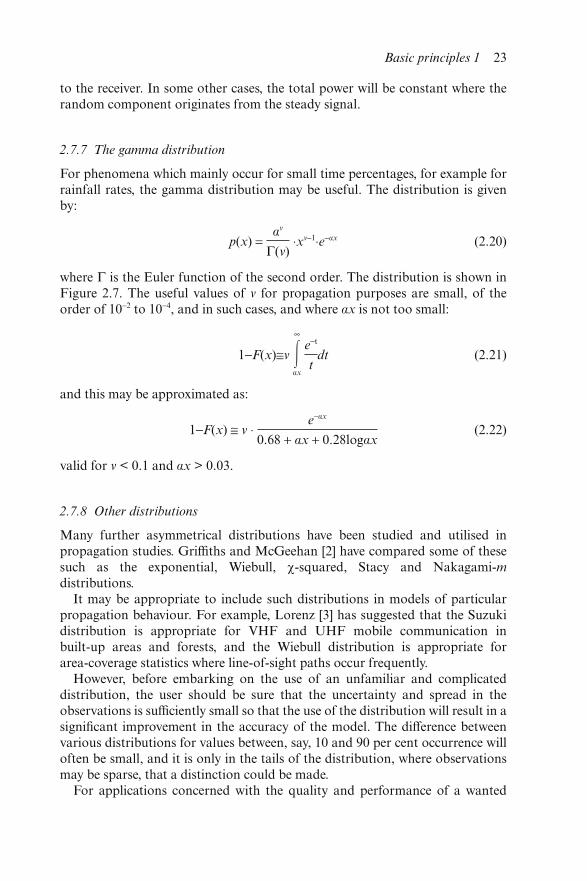
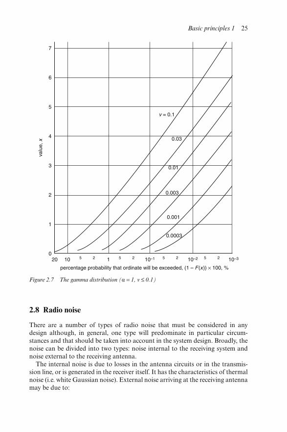
where Γ is the Euler function of the second order. The distribution is shown inFigure 2.7. The useful values of ν for propagation purposes are small, of theorder of 10−2 to 10−4, and in such cases, and where αx is not too small:
1−F(x)≅ν �∞
αx
e−t
tdt (2.21)
and this may be approximated as:
1−F(x) ≅ ν ⋅ e−αx
0.68 + αx + 0.28logαx(2.22)
valid for ν < 0.1 and αx > 0.03.
2.7.8 Other distributions
Many further asymmetrical distributions have been studied and utilised inpropagation studies. Griffiths and McGeehan [2] have compared some of thesesuch as the exponential, Wiebull, χ-squared, Stacy and Nakagami-mdistributions.
It may be appropriate to include such distributions in models of particularpropagation behaviour. For example, Lorenz [3] has suggested that the Suzukidistribution is appropriate for VHF and UHF mobile communication inbuilt-up areas and forests, and the Wiebull distribution is appropriate forarea-coverage statistics where line-of-sight paths occur frequently.
However, before embarking on the use of an unfamiliar and complicateddistribution, the user should be sure that the uncertainty and spread in theobservations is sufficiently small so that the use of the distribution will result in asignificant improvement in the accuracy of the model. The difference betweenvarious distributions for values between, say, 10 and 90 per cent occurrence willoften be small, and it is only in the tails of the distribution, where observationsmay be sparse, that a distinction could be made.
For applications concerned with the quality and performance of a wanted
Basic principles 1 23
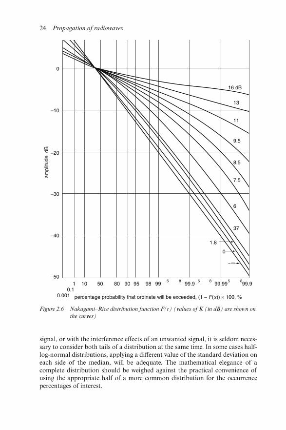
signal, or with the interference effects of an unwanted signal, it is seldom neces-sary to consider both tails of a distribution at the same time. In some cases half-log-normal distributions, applying a different value of the standard deviation oneach side of the median, will be adequate. The mathematical elegance of acomplete distribution should be weighed against the practical convenience ofusing the appropriate half of a more common distribution for the occurrencepercentages of interest.
Figure 2.6 Nakagami–Rice distribution function F(r) (values of K (in dB) are shown on
the curves)
24 Propagation of radiowaves
2.8 Radio noise
There are a number of types of radio noise that must be considered in anydesign although, in general, one type will predominate in particular circum-stances and that should be taken into account in the system design. Broadly, thenoise can be divided into two types: noise internal to the receiving system andnoise external to the receiving antenna.
The internal noise is due to losses in the antenna circuits or in the transmis-sion line, or is generated in the receiver itself. It has the characteristics of thermalnoise (i.e. white Gaussian noise). External noise arriving at the receiving antennamay be due to:
Figure 2.7 The gamma distribution (α = 1, ν ≤ 0.1)
Basic principles 1 25
(i) atmospheric noise generated by lightning discharges, or resulting fromabsorption by atmospheric gases (sky noise);
(ii) the cosmic background, primarily from the Galaxy, or from the sun;(iii) broadband man-made noise generated by machinery, power systems etc.
In general, noise is broadband, with an intensity varying only slowly with fre-quency, but in some cases, e.g. noise emanating from computer systems, theintensity may have considerable frequency variability.
The noise power due to external sources, pn, can conveniently be expressed asa noise factor, fa, which is the ratio of the noise power to the correspondingthermal noise, or as a noise temperature, ta, thus:
fa = Pn
kt0b =
ta
t0
(2.23)
where k is Boltzmann’s constant = 1.38 × 10⁻²³J K−1, t0 is the reference tempera-ture, taken as 288 K and b is the noise bandwidth of the receiving system in Hz.
Note there is some confusion in the currently used terminology but here fa
is the numerical noise factor, and the term noise figure, Fa, is used for thelogarithmic ratio, so that:
Fa = 10 log fa (2.24)
The available noise power in decibels above 1 W is given by:
Pn = Fa + B − 204 dBW (2.25)
where B = 10 log b.When measured with a halfwave dipole in free space the corresponding value
of the RMS field strength is given by:
En = Fa + 20 log fMHz + B − 99 dB(μV m−1) (2.26)
and for a short vertical grounded monopole by (taking account of the effect ofthe ground as mentioned in Section 2.5):
En = Fa + 20 log fMHz + B − 95.5 dB(μV m−1) (2.27)
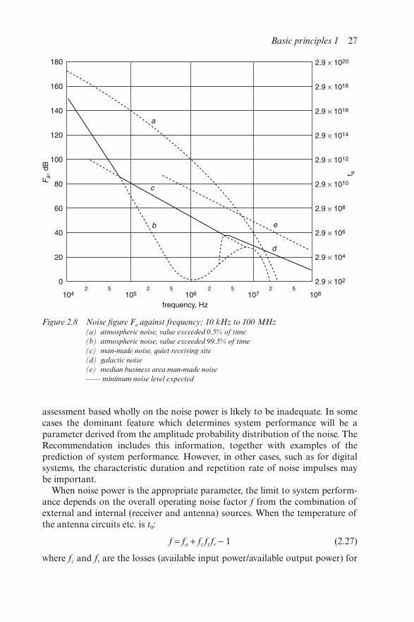
Minimum, and some maximum, values for the external noise figures are shownin Figures 2.8 and 2.9. Generally, one type of noise will predominate, but wherethe contributions of more than one type of noise are comparable, the noisefactors (not the figures in decibels) should be added. Atmospheric noise due tolightning varies with location on the earth, season, time of day and frequency.Maps and frequency correction charts are given in ITU-R RecommendationP.372. Man-made noise varies with the extent of man-made activity and the useof machinery, electrical equipment etc. The relationship for a range of environ-ments is also given in the Recommendation. Note that some care may be neededto ensure that an appropriate curve is selected since the noise generated, forexample in a business area, may differ from country to country.
Both atmospheric and man-made noise are impulsive in character, and an
26 Propagation of radiowaves
assessment based wholly on the noise power is likely to be inadequate. In somecases the dominant feature which determines system performance will be aparameter derived from the amplitude probability distribution of the noise. TheRecommendation includes this information, together with examples of theprediction of system performance. However, in other cases, such as for digitalsystems, the characteristic duration and repetition rate of noise impulses maybe important.
When noise power is the appropriate parameter, the limit to system perform-ance depends on the overall operating noise factor f from the combination ofexternal and internal (receiver and antenna) sources. When the temperature ofthe antenna circuits etc. is t0:
f = fa + fc ft fr − 1 (2.27)
where fc and ft are the losses (available input power/available output power) for
Figure 2.8 Noise figure Fa against frequency; 10 kHz to 100 MHz(a) atmospheric noise, value exceeded 0.5% of time
(b) atmospheric noise, value exceeded 99.5% of time
(c) man-made noise, quiet receiving site
(d) galactic noise
(e) median business area man-made noise
—— minimum noise level expected
Basic principles 1 27
the antenna circuit and transmission line, respectively; fr is the noise factor ofthe receiver and fa is the noise factor due to the external noise sources.
2.9 Link power budgets
In the design of a communications system it will be necessary to ensure that thelevel of the received signal is adequate to provide the required quality of service.
The way in which this is done will depend on the details of the system and therequirements for the application.
In some cases, where the performance of a typical, or minimum specification,receiver is assumed and where there may be no control over some of the antennacharacteristics, a minimum usable field strength or reference minimum fieldstrength may be specified. This has been done for some broadcast and mobileservices. Assuming that the reception approximately corresponds to free-spaceconditions, e.g. not too close to the ground, which is implicit in this kind ofcharacterisation, Eqns 2.3 and 2.5 may be used to relate the field strength to aminimum available power, pr,min, in the typical receiver. Then a simplified linkpower budget, with the terms expressed in decibels, may be determined:
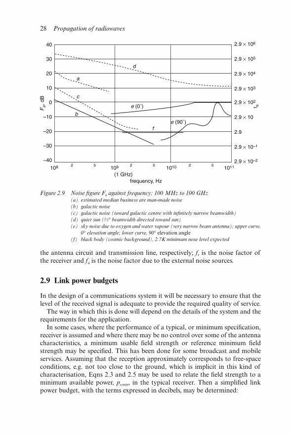
Figure 2.9 Noise figure Fa against frequency; 100 MHz to 100 GHz(a) estimated median business are man-made noise
(b) galactic noise
(c) galactic noise (toward galactic centre with infinitely narrow beamwidth)
(d) quiet sun (½° beamwidth directed toward sun)
(e) sky noise due to oxygen and water vapour (very narrow beam antenna); upper curve,
0° elevation angle; lower curve, 90° elevation angle(f) black body (cosmic background), 2.7K minimum nose level expected
28 Propagation of radiowaves
Pt + Gt = Lb + Pr, min (2.28)
In other cases it will be appropriate to consider the performance of individualreceiving installations and to specify the required signal/noise ratio, RS/N. Wherethe performance is limited by the effective receiver noise factor, the link powerbudget becomes:
Pt + Gt = Lb + RS/N + Fa + B − 204 (2.29)
where Pt is in dBW.In practical circumstances these skeleton link budgets would have to be
refined by adding antenna feeder losses etc. For digital systems other aspects,such as the impulse response of the channel, will also have to be considered, inaddition to the transmission loss.
In all cases, however, the basic transmission loss, Lb, is a determining termwhich will be obtained from propagation prediction or modelling. As describedin Section 2.6, the basic transmission loss includes losses due to propagationeffects in addition to the free-space spreading loss. These additional lossesshould be determined for the time percentage used in defining the quality ofservice. Typically, a service quality will be specified for 95, 99 or 99.99 per centof the time or location etc., and the channel fading or the incidence of the effectat this percentage should be determined. This will be the subject of laterchapters.
The procedure may, if necessary, be extended still further to include the prob-able error of the prediction of transmission loss which may be due, for example,to the sampling involved in establishing the method. Where no allowance for thisis included, the prediction has a confidence level of 50 per cent, since one half ofthe specific cases encountered are likely in practice to be below the predictedlevel. An assessment may be made of the probable error and, by applying anormal distribution, an allowance may be made for any other desired confidencelevel. This has been described by Barclay [4].
2.9.1 Fading allowances
In some cases, for service planning, the specified signal-to-noise ratio for therequired grade of service will probably include an allowance for the rapid fadingwhich will affect the intelligibility or the bit error ratio of the system. It may stillbe necessary to allow for other variations (hour-to-hour, day-to-day, location-to-location) of both signal and noise, which are likely to be log-normally dis-tributed, but uncorrelated. This may be done by determining the basic transmis-sion loss for median conditions and then adding a fading allowance, assuming alog-normal distribution with a variance, σ2, obtained by adding the variances ofeach contributing distribution, i.e.
σ2 = σ12 + σ2
2 + . . . (2.30)
Basic principles 1 29
2.10 Diversity
The allowance for propagation effects necessary to achieve a good grade ofservice may demand economically prohibitive transmitter powers and antennagains. In any case, the use of excessive radiated power conflicts with the need forgood spectrum utilisation. Techniques for overcoming this problem include cod-ing and diversity. Particularly for circuits with rapid fading, such as those whereRayleigh or Rician fading dominates, copies of the signal with the same charac-teristics are available displaced in time, position, frequency or, for some types ofpropagation, with angle of arrival or orthogonal polarisation. For example, asignal message may be repeated later in time if, when first transmitted, a fadehad reduced the signal-to-noise ratio. For digital systems this process may beautomated by the use of an error-detecting code using a method of automaticrepeat requests (ARQ) if errors are detected in the received signal. More moderntechniques use sophisticated error-correction and error-detection codes to com-bat the effects of fading, and these may take account of the expected patterns oferror occurrence (e.g. where errors occur in bursts). Spread-spectrum signals,both direct-sequence and frequency-hopping, employ techniques to take advan-tage of the frequency-selective nature of fading, and this is discussed in laterchapters.
Diversity techniques utilise two or more samples of the signal obtained fromseparated antennas, or sometimes from duplicated transmissions on several fre-quencies. These signals are then combined in the receiver to produce an outputwith a smaller fading variability. Signals may be combined by techniques suchas:
(i) selection of the stronger or strongest(ii) combining the output of channels with equal gain(iii) weighting the combination according to the signal-to-noise ratio of the
channel (maximal ratio combining).
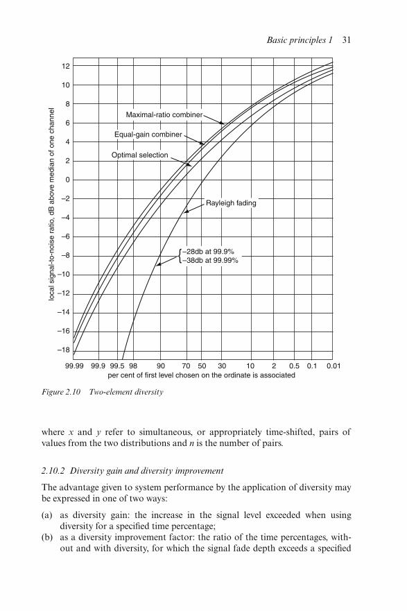
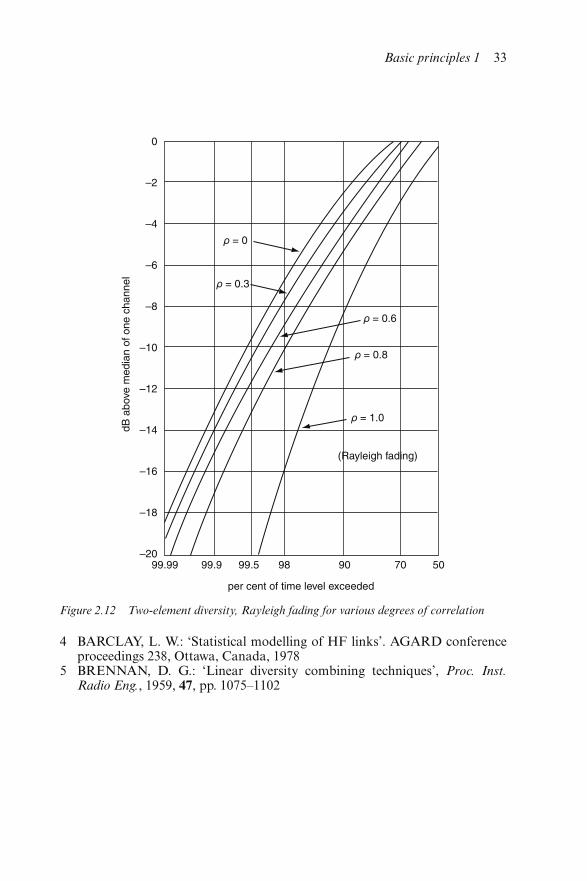
Figure 2.10 shows the distributions for two-element diversity [5], where the sig-nals are uncorrelated and each has a Rayleigh distribution, for various methodsof combination. The corresponding distribution for four-channel diversity (asmight be employed for tropospheric scatter systems) is shown in Figure 2.11.In fact, a substantial advantage is still obtained if the signals are partiallycorrelated. Figure 2.12 shows, for two-element-selection diversity, the effect ofvarying the correlation coefficient.
2.10.1 Correlation coefficient
The correlation coefficient is obtained as:
r = �{(x − x)(y − y)}
��(x − x)2�(y − y)2�0.5 =
�xy − nxy
nσxσy
(2.31)
30 Propagation of radiowaves
where x and y refer to simultaneous, or appropriately time-shifted, pairs ofvalues from the two distributions and n is the number of pairs.
2.10.2 Diversity gain and diversity improvement
The advantage given to system performance by the application of diversity maybe expressed in one of two ways:
(a) as diversity gain: the increase in the signal level exceeded when usingdiversity for a specified time percentage;
(b) as a diversity improvement factor: the ratio of the time percentages, with-out and with diversity, for which the signal fade depth exceeds a specified
Figure 2.10 Two-element diversity
Basic principles 1 31
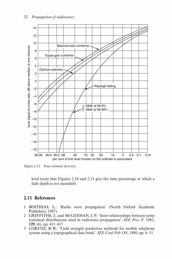
level (note that Figures 2.10 and 2.11 give the time percentage at which afade depth is not exceeded).
2.11 References
1 BOITHIAS, L.: ‘Radio wave propagation’ (North Oxford AcademicPublishers, 1987)
2 GRIFFITHS, J., and McGEEHAN, J. P.: ‘Inter-relationships between somestatistical distributions used in radiowave propagation’, IEE Proc F, 1982,129, (6), pp. 411–417
3 LORENZ, R.W.: ‘Field strength prediction methods for mobile telephonesystem using a topographical data bank’. IEE Conf Pub 188, 1980, pp. 6–11
Figure 2.11 Four-element diversity
32 Propagation of radiowaves
4 BARCLAY, L. W.: ‘Statistical modelling of HF links’. AGARD conferenceproceedings 238, Ottawa, Canada, 1978
5 BRENNAN, D. G.: ‘Linear diversity combining techniques’, Proc. Inst.Radio Eng., 1959, 47, pp. 1075–1102
Figure 2.12 Two-element diversity, Rayleigh fading for various degrees of correlation
Basic principles 1 33

Chapter 3
Basic principles 2
David Bacon
3.1 Vector nature of radiowaves
Although for many purposes a radiowave can be treated simply as a power flow,there are other situations where it is necessary to take into account the fact thatit consists of vector fields.
3.1.1 Qualitative description of the plane wave
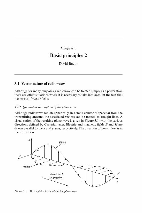
Although radiowaves radiate spherically, in a small volume of space far from thetransmitting antenna the associated vectors can be treated as straight lines. Avisualisation of the resulting plane wave is given in Figure 3.1, with the variousdirections defined by Cartesian axes. Electric and magnetic fields E and H aredrawn parallel to the x and y axes, respectively. The direction of power flow is inthe z direction.
Figure 3.1 Vector fields in an advancing plane wave
The E and H field sinusoids are in phase with each other, and the completepattern moves in the z direction. Thus the E and H fields vary in both space andtime. Although in Figure 3.1 the field vectors are drawn from a single z axis, infact they fill and are equal over any xy plane.
Two useful concepts in propagation studies are:
Ray: a ray is a mathematically thin line indicating the direction of propagation.In Figure 3.1, any line for which x and y are both constant can be viewed as aray.
Wavefront: a wavefront is any surface which is everywhere normal to the direc-tion of propagation. In Figure 3.1, any plane for which z is constant can beviewed as a wavefront.
3.1.2 Complex phasor notation
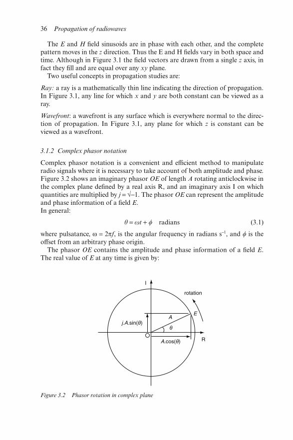
Complex phasor notation is a convenient and efficient method to manipulateradio signals where it is necessary to take account of both amplitude and phase.Figure 3.2 shows an imaginary phasor OE of length A rotating anticlockwise inthe complex plane defined by a real axis R, and an imaginary axis I on whichquantities are multiplied by j = √−1. The phasor OE can represent the amplitudeand phase information of a field E.In general:
θ = ωt + radians (3.1)
where pulsatance, ω = 2πf, is the angular frequency in radians s−1, and is theoffset from an arbitrary phase origin.
The phasor OE contains the amplitude and phase information of a field E.The real value of E at any time is given by:
Figure 3.2 Phasor rotation in complex plane
36 Propagation of radiowaves
Re(E) = A cos (θ) V m−1 (3.2)
and the so-called imaginary component of E is given by:
Im(E) = j.A sin (θ) V m−1 (3.3)
Complete information on the amplitude and phase of E is contained in the realand imaginary components, and hence E is fully defined by:
E = A {cos (θ) + j.sin (θ)} V m−1 (3.4)
Following the identity cos(x) + j.sin(x) = exp(jx), E can alternatively beexpressed in the complex exponential form:
E = A exp (j.θ) V m−1 (3.5)
3.1.3 The sense of time and space
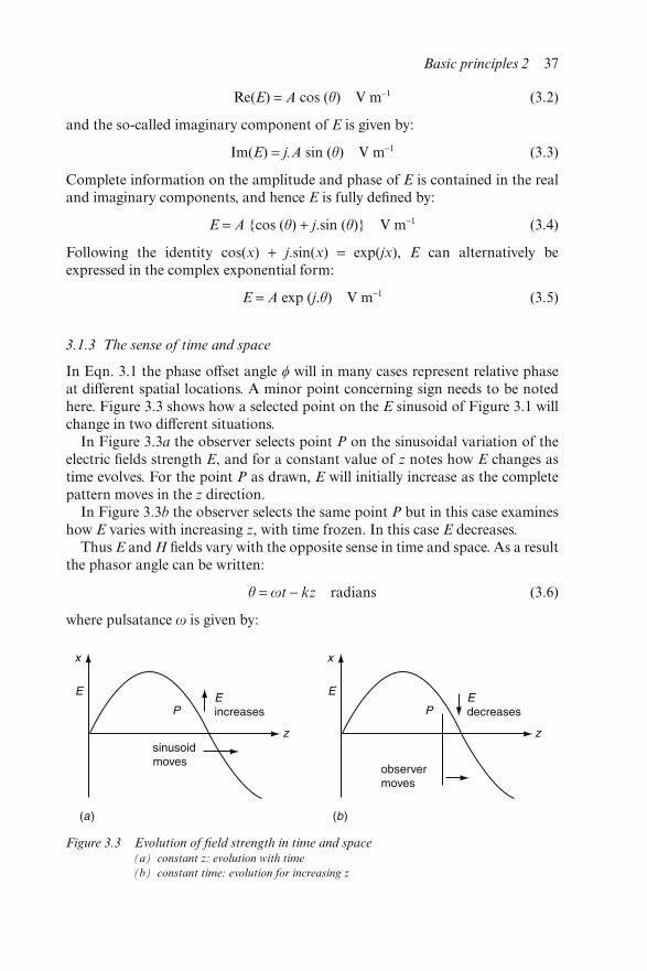
In Eqn. 3.1 the phase offset angle will in many cases represent relative phaseat different spatial locations. A minor point concerning sign needs to be notedhere. Figure 3.3 shows how a selected point on the E sinusoid of Figure 3.1 willchange in two different situations.
In Figure 3.3a the observer selects point P on the sinusoidal variation of theelectric fields strength E, and for a constant value of z notes how E changes astime evolves. For the point P as drawn, E will initially increase as the completepattern moves in the z direction.
In Figure 3.3b the observer selects the same point P but in this case examineshow E varies with increasing z, with time frozen. In this case E decreases.
Thus E and H fields vary with the opposite sense in time and space. As a resultthe phasor angle can be written:
θ = ωt − kz radians (3.6)
where pulsatance ω is given by:
Figure 3.3 Evolution of field strength in time and space(a) constant z: evolution with time
(b) constant time: evolution for increasing z
Basic principles 2 37
ω = 2πf radians s−1 (3.6a)
and wavenumber k is given by:
k = 2π/λ radians m−1 (3.6b)
with f = frequency in Hz and λ = wavelength in metres.Thus the temporal and spatial variation of field strength E for the coordinate
system used in Figure 3.1 can be expressed efficiently in complex form by:
E = exp (j.[ωt − kz]) V m−1 (3.7)
noting that for a plane wave E is constant with x and y.If only the spatial variation of E at a given instance of time is of interest, then
t can be set to zero, and E is given by:
E = exp (− j.kz) V m−1 (3.8)
This form for the complex representation of a signal is widely used in radiowavepropagation.
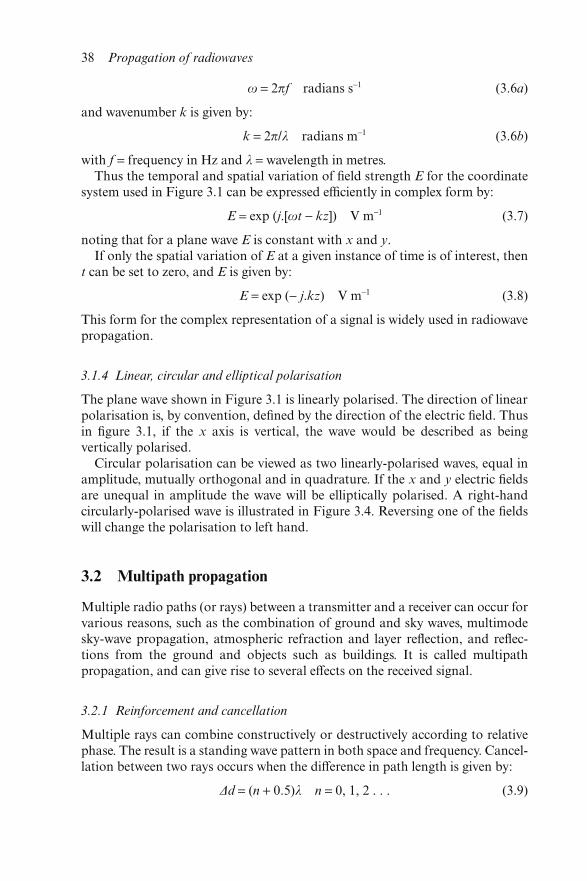
3.1.4 Linear, circular and elliptical polarisation
The plane wave shown in Figure 3.1 is linearly polarised. The direction of linearpolarisation is, by convention, defined by the direction of the electric field. Thusin figure 3.1, if the x axis is vertical, the wave would be described as beingvertically polarised.
Circular polarisation can be viewed as two linearly-polarised waves, equal inamplitude, mutually orthogonal and in quadrature. If the x and y electric fieldsare unequal in amplitude the wave will be elliptically polarised. A right-handcircularly-polarised wave is illustrated in Figure 3.4. Reversing one of the fieldswill change the polarisation to left hand.
3.2 Multipath propagation
Multiple radio paths (or rays) between a transmitter and a receiver can occur forvarious reasons, such as the combination of ground and sky waves, multimodesky-wave propagation, atmospheric refraction and layer reflection, and reflec-tions from the ground and objects such as buildings. It is called multipathpropagation, and can give rise to several effects on the received signal.
3.2.1 Reinforcement and cancellation
Multiple rays can combine constructively or destructively according to relativephase. The result is a standing wave pattern in both space and frequency. Cancel-lation between two rays occurs when the difference in path length is given by:
Δd = (n + 0.5)λ n = 0, 1, 2 . . . (3.9)
38 Propagation of radiowaves
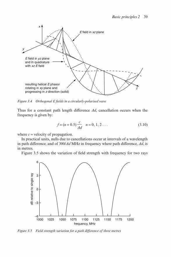
Thus for a constant path length difference Δd, cancellation occurs when thefrequency is given by:
f = (n + 0.5)c
Δdn = 0, 1, 2 . . . (3.10)
where c = velocity of propagation.In practical units, nulls due to cancellations occur at intervals of a wavelength
in path difference, and of 300/Δd MHz in frequency where path difference, Δd, isin metres.
Figure 3.5 shows the variation of field strength with frequency for two rays
Figure 3.4 Orthogonal E fields in a circularly-polarised wave
Figure 3.5 Field strength variation for a path difference of three metres
Basic principles 2 39
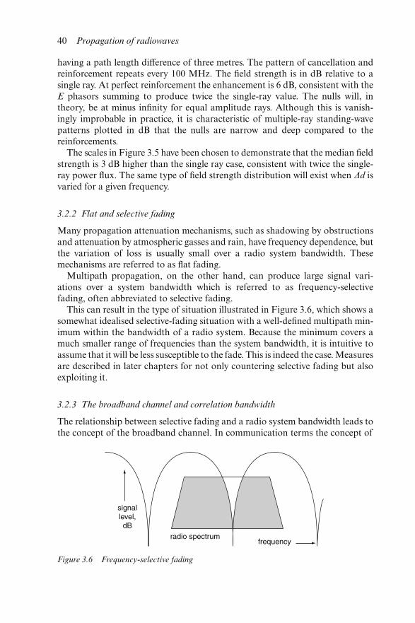
having a path length difference of three metres. The pattern of cancellation andreinforcement repeats every 100 MHz. The field strength is in dB relative to asingle ray. At perfect reinforcement the enhancement is 6 dB, consistent with theE phasors summing to produce twice the single-ray value. The nulls will, intheory, be at minus infinity for equal amplitude rays. Although this is vanish-ingly improbable in practice, it is characteristic of multiple-ray standing-wavepatterns plotted in dB that the nulls are narrow and deep compared to thereinforcements.
The scales in Figure 3.5 have been chosen to demonstrate that the median fieldstrength is 3 dB higher than the single ray case, consistent with twice the single-ray power flux. The same type of field strength distribution will exist when Δd isvaried for a given frequency.
3.2.2 Flat and selective fading
Many propagation attenuation mechanisms, such as shadowing by obstructionsand attenuation by atmospheric gasses and rain, have frequency dependence, butthe variation of loss is usually small over a radio system bandwidth. Thesemechanisms are referred to as flat fading.
Multipath propagation, on the other hand, can produce large signal vari-ations over a system bandwidth which is referred to as frequency-selectivefading, often abbreviated to selective fading.
This can result in the type of situation illustrated in Figure 3.6, which shows asomewhat idealised selective-fading situation with a well-defined multipath min-imum within the bandwidth of a radio system. Because the minimum covers amuch smaller range of frequencies than the system bandwidth, it is intuitive toassume that it will be less susceptible to the fade. This is indeed the case. Measuresare described in later chapters for not only countering selective fading but alsoexploiting it.
3.2.3 The broadband channel and correlation bandwidth
The relationship between selective fading and a radio system bandwidth leads tothe concept of the broadband channel. In communication terms the concept of
Figure 3.6 Frequency-selective fading
40 Propagation of radiowaves
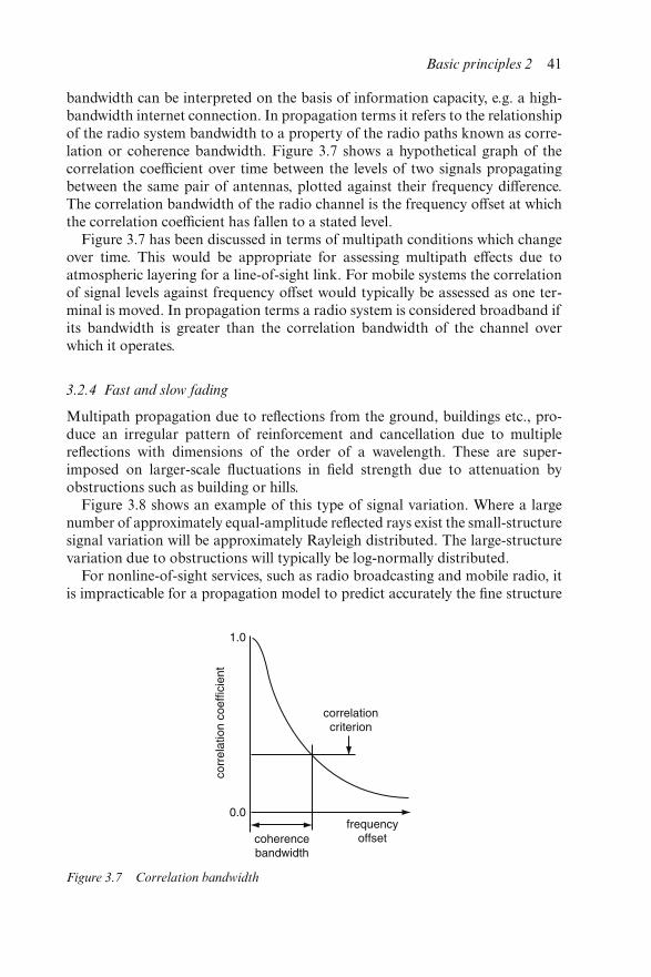
bandwidth can be interpreted on the basis of information capacity, e.g. a high-bandwidth internet connection. In propagation terms it refers to the relationshipof the radio system bandwidth to a property of the radio paths known as corre-lation or coherence bandwidth. Figure 3.7 shows a hypothetical graph of thecorrelation coefficient over time between the levels of two signals propagatingbetween the same pair of antennas, plotted against their frequency difference.The correlation bandwidth of the radio channel is the frequency offset at whichthe correlation coefficient has fallen to a stated level.
Figure 3.7 has been discussed in terms of multipath conditions which changeover time. This would be appropriate for assessing multipath effects due toatmospheric layering for a line-of-sight link. For mobile systems the correlationof signal levels against frequency offset would typically be assessed as one ter-minal is moved. In propagation terms a radio system is considered broadband ifits bandwidth is greater than the correlation bandwidth of the channel overwhich it operates.
3.2.4 Fast and slow fading
Multipath propagation due to reflections from the ground, buildings etc., pro-duce an irregular pattern of reinforcement and cancellation due to multiplereflections with dimensions of the order of a wavelength. These are super-imposed on larger-scale fluctuations in field strength due to attenuation byobstructions such as building or hills.
Figure 3.8 shows an example of this type of signal variation. Where a largenumber of approximately equal-amplitude reflected rays exist the small-structuresignal variation will be approximately Rayleigh distributed. The large-structurevariation due to obstructions will typically be log-normally distributed.
For nonline-of-sight services, such as radio broadcasting and mobile radio, itis impracticable for a propagation model to predict accurately the fine structure
Figure 3.7 Correlation bandwidth
Basic principles 2 41
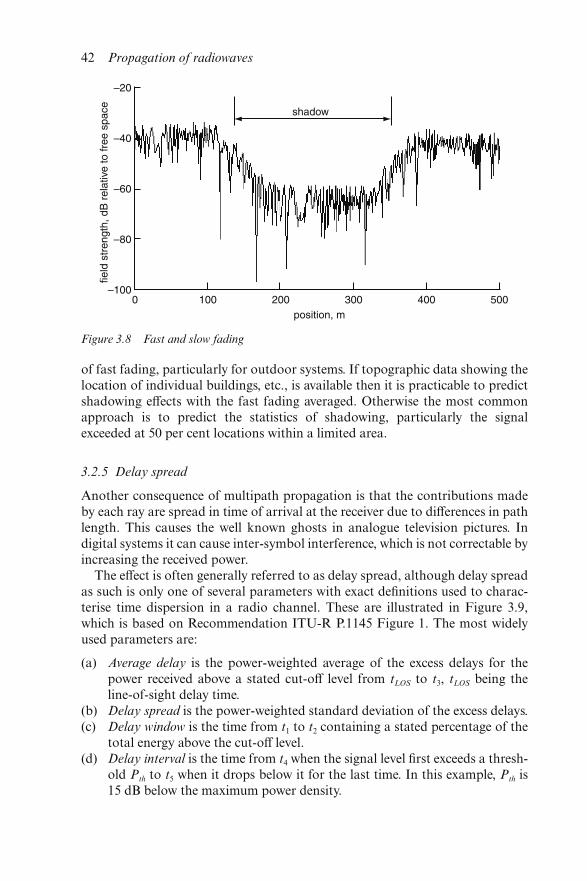
of fast fading, particularly for outdoor systems. If topographic data showing thelocation of individual buildings, etc., is available then it is practicable to predictshadowing effects with the fast fading averaged. Otherwise the most commonapproach is to predict the statistics of shadowing, particularly the signalexceeded at 50 per cent locations within a limited area.
3.2.5 Delay spread
Another consequence of multipath propagation is that the contributions madeby each ray are spread in time of arrival at the receiver due to differences in pathlength. This causes the well known ghosts in analogue television pictures. Indigital systems it can cause inter-symbol interference, which is not correctable byincreasing the received power.
The effect is often generally referred to as delay spread, although delay spreadas such is only one of several parameters with exact definitions used to charac-terise time dispersion in a radio channel. These are illustrated in Figure 3.9,which is based on Recommendation ITU-R P.1145 Figure 1. The most widelyused parameters are:
(a) Average delay is the power-weighted average of the excess delays for thepower received above a stated cut-off level from tLOS to t3, tLOS being theline-of-sight delay time.
(b) Delay spread is the power-weighted standard deviation of the excess delays.(c) Delay window is the time from t1 to t2 containing a stated percentage of the
total energy above the cut-off level.(d) Delay interval is the time from t4 when the signal level first exceeds a thresh-
old Pth to t5 when it drops below it for the last time. In this example, Pth is15 dB below the maximum power density.
Figure 3.8 Fast and slow fading
42 Propagation of radiowaves
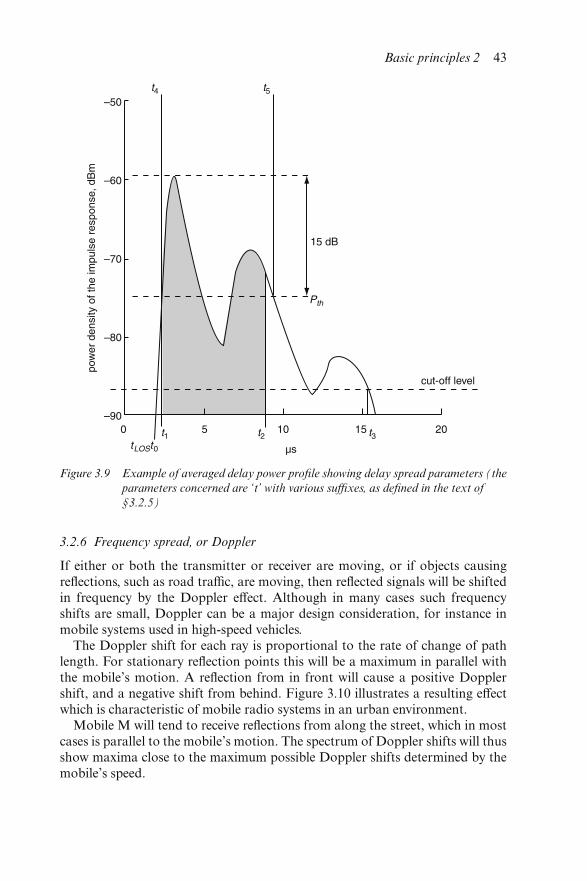
3.2.6 Frequency spread, or Doppler
If either or both the transmitter or receiver are moving, or if objects causingreflections, such as road traffic, are moving, then reflected signals will be shiftedin frequency by the Doppler effect. Although in many cases such frequencyshifts are small, Doppler can be a major design consideration, for instance inmobile systems used in high-speed vehicles.
The Doppler shift for each ray is proportional to the rate of change of pathlength. For stationary reflection points this will be a maximum in parallel withthe mobile’s motion. A reflection from in front will cause a positive Dopplershift, and a negative shift from behind. Figure 3.10 illustrates a resulting effectwhich is characteristic of mobile radio systems in an urban environment.
Mobile M will tend to receive reflections from along the street, which in mostcases is parallel to the mobile’s motion. The spectrum of Doppler shifts will thusshow maxima close to the maximum possible Doppler shifts determined by themobile’s speed.
Figure 3.9 Example of averaged delay power profile showing delay spread parameters (the
parameters concerned are ‘t’ with various suffixes, as defined in the text of
§3.2.5)
Basic principles 2 43
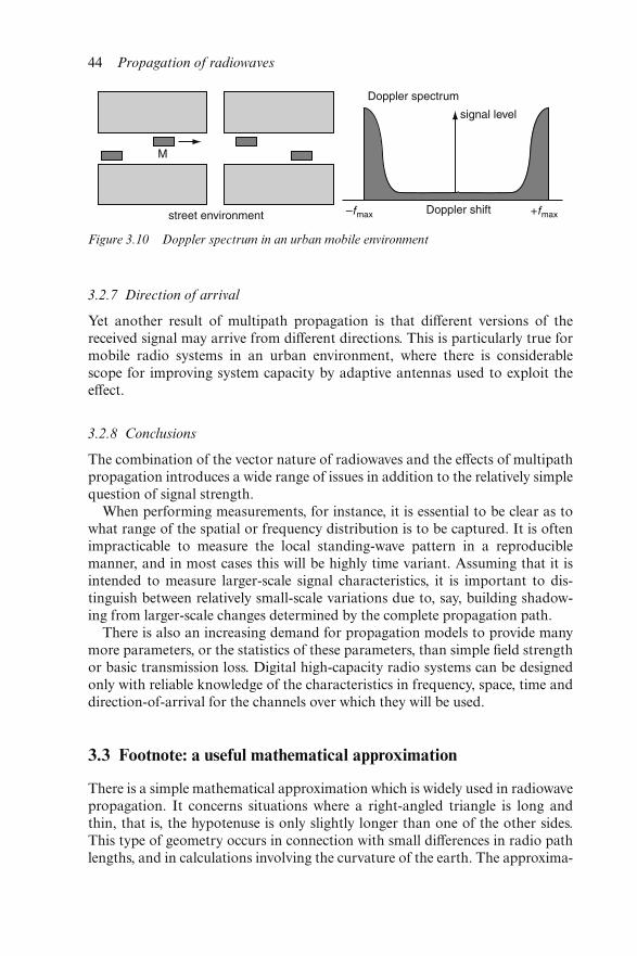
3.2.7 Direction of arrival
Yet another result of multipath propagation is that different versions of thereceived signal may arrive from different directions. This is particularly true formobile radio systems in an urban environment, where there is considerablescope for improving system capacity by adaptive antennas used to exploit theeffect.
3.2.8 Conclusions
The combination of the vector nature of radiowaves and the effects of multipathpropagation introduces a wide range of issues in addition to the relatively simplequestion of signal strength.
When performing measurements, for instance, it is essential to be clear as towhat range of the spatial or frequency distribution is to be captured. It is oftenimpracticable to measure the local standing-wave pattern in a reproduciblemanner, and in most cases this will be highly time variant. Assuming that it isintended to measure larger-scale signal characteristics, it is important to dis-tinguish between relatively small-scale variations due to, say, building shadow-ing from larger-scale changes determined by the complete propagation path.
There is also an increasing demand for propagation models to provide manymore parameters, or the statistics of these parameters, than simple field strengthor basic transmission loss. Digital high-capacity radio systems can be designedonly with reliable knowledge of the characteristics in frequency, space, time anddirection-of-arrival for the channels over which they will be used.
3.3 Footnote: a useful mathematical approximation
There is a simple mathematical approximation which is widely used in radiowavepropagation. It concerns situations where a right-angled triangle is long andthin, that is, the hypotenuse is only slightly longer than one of the other sides.This type of geometry occurs in connection with small differences in radio pathlengths, and in calculations involving the curvature of the earth. The approxima-
Figure 3.10 Doppler spectrum in an urban mobile environment
44 Propagation of radiowaves
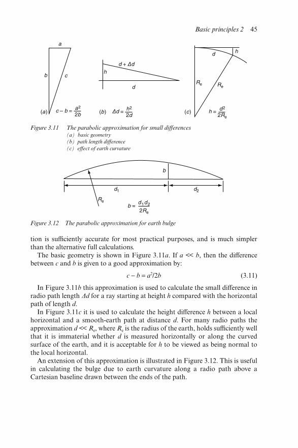
tion is sufficiently accurate for most practical purposes, and is much simplerthan the alternative full calculations.
The basic geometry is shown in Figure 3.11a. If a << b, then the differencebetween c and b is given to a good approximation by:
c − b = a2/2b (3.11)
In Figure 3.11b this approximation is used to calculate the small difference inradio path length Δd for a ray starting at height h compared with the horizontalpath of length d.
In Figure 3.11c it is used to calculate the height difference h between a localhorizontal and a smooth-earth path at distance d. For many radio paths theapproximation d << Re, where Re is the radius of the earth, holds sufficiently wellthat it is immaterial whether d is measured horizontally or along the curvedsurface of the earth, and it is acceptable for h to be viewed as being normal tothe local horizontal.
An extension of this approximation is illustrated in Figure 3.12. This is usefulin calculating the bulge due to earth curvature along a radio path above aCartesian baseline drawn between the ends of the path.
Figure 3.11 The parabolic approximation for small differences(a) basic geometry
(b) path length difference
(c) effect of earth curvature
Figure 3.12 The parabolic approximation for earth bulge
Basic principles 2 45

Chapter 4
Propagation data requirements forradiocommunications system planning
Tim Hewitt
4.1 Introduction
It is neither economically realistic nor spectrally efficient to engineer a radio-communications system to the extent that it can be guaranteed to work for 100per cent of the time, and realistic allowances have to be made for equipmentfailures, propagation problems, and interference. When planning a system it istherefore necessary to have design targets for the maximum percentages of timefor which the circuit may be interrupted, or its error performance degraded.
The amount of time for which a degraded level of service can be acceptedis dependent on the particular application. High-grade telecommunicationssystems are very tightly specified in this respect, typically needing to be fullyoperational for all but few hundredths of a per cent of the time. Even localaccess radio systems generally need to work to 99.99 per cent of the time, orbetter. Broadcasting is more tolerant, with perhaps 0.1 per cent of time beingallowed for interruptions. However, mobile networks, which live in aninterference-dominated environment in which performance is statistically lesscertain, are normally designed for median conditions and are not so concernedabout the smaller time percentages.
Once total allowable time percentages for degraded performance and outagehave been decided, they generally need to be apportioned (not necessarilyequally) between equipment failures, propagation effects and interference. Fur-thermore, for example, the propagation allowances may need to be furtherapportioned between several tandem hops in a radio network. In some cases thiscan result in very small time percentages indeed being allowed for propagationand interference effects on each individual radio hop. The system designer isthen working with the tails of the wanted signal and interference propagationdistributions, and with all the uncertainties that these represent.
In practice, the quality of a digital radio circuit is defined and/or measured intwo ways, i.e. by its availability for the transport of information, and by its errorperformance in terms of the number of errors that occur while it is available.These two quality objectives are discussed in greater detail below.
Designing radio systems to recommended performance and availability tar-gets raises a number of issues relating to the types of propagation informationrequired. Unfortunately, as things currently stand, the expectations of the designengineer cannot always be matched by the available propagation data and pre-diction models. It is therefore necessary for the designer to appreciate the limita-tions of current propagation knowledge, and to devise pragmatic solutions thatwill allow the design work to move forward within the constraints of the datathat is available.
The notes below explore the general issues associated with performance andavailability requirements for modern digital radiocommunications systems, asset out within the relevant ITU-R Recommendations. The emphasis is onexamples that illustrate the various propagation issues that can arise, and thenotes are not intended to be a tutorial on radio link design.
4.2 Quality parameters for radiocommunications circuits
4.2.1 Key terms and definitions
When discussing radio link design it is necessary to get a little involved in thelanguage of that art. In the context of this present discussion there are fourterms that are of particular relevance to the planning of digital radio-communications systems:
(i) Errored seconds (ES) are seconds during which errors occur in the informa-tion bits being carried. The errors will normally be in the context of thebaseband (information) signal rather than the RF channel. Modern digitalsystems with adaptive demodulators and error correction can do much tocorrect the basic transmission errors. Trade-offs between system sophisti-cation and fading and interference margins are therefore available, and arenowadays used to excellent effect.
(ii) Severely errored seconds (SES) are seconds during which the error rate(typically at the 64 kbit s−1 level) within the 1 s period exceeds a pre-definedthreshold, normally one error in 103 bits.
(iii) Error performance is the measure of the transmission quality that a circuitshould, or does, achieve while it is available for the transport of informa-tion. For digital circuits, performance is described in terms of the erroredseconds ratio (ESR) and the severely errored seconds ratio. These are theratios of errored and severely errored seconds, respectively, to the totalnumber of available seconds, usually in any month.
(iv) Availability is the percentage of the total time during which the circuitshould be, or is, delivering the required performance, i.e. the total time that
48 Propagation of radiowaves
it is not out of service due to equipment, propagation or interferenceproblems. For digital circuits, a period of unavailability begins at the startof a sequence of ten consecutive SES, and ceases at the start of the next tensecond without any SES.
Recommendation ITU-R F.557-4 states ‘. . . that in the estimation of unavail-ability, one must include all causes which are statistically predictable, uninten-tional and resulting from the radio equipment, power supplies, propagation,interference, and from auxiliary equipment and human activity, and that the esti-mate of unavailability should include consideration of the mean time to restore’.
This indicates that the overall recommended unavailability allowance must beapportioned between these different causes. This might imply that both thefading of the wanted signal and the statistics of unwanted interference must beanalysed together to ensure that the quality objectives are met. How the allow-ances are apportioned between the different causes is a fundamental decision forthe design engineer.
It is therefore necessary to have propagation models to predict the propaga-tion conditions on the wanted path (e.g. Recommendation ITU-R P.530 forterrestrial paths or Recommendation ITU-R P.618 for earth–space paths), aswell as those to predict the levels of interference between the wanted system andother cochannel systems (e.g. Recommendation ITU-R P.452). These importantpropagation recommendations are described in other chapters.
4.2.2 Related propagation issues
Ideally, the design engineer who is planning the system should have availablepropagation data that will enable him to demonstrate that the design will meetboth the performance and the availability objectives.
This provides the propagation engineer with many significant challenges. Fora digital radio circuit the concept of availability, as defined above, poses specialproblems in the context of propagation data.
Figure 4.1 shows a short period of transmission on a digital radio link. Dur-ing this period fading is occurring, sometimes to a significant extent. Within thefirst 24 seconds the fading is significant, but the event durations are short andthere are no continuous periods of SES of ten seconds or longer that wouldcount as unavailability, as defined above. All of the errors in this period willtherefore count towards the allowance for error performance degradation, i.e.they will contribute to the ESR and/or the SESR. From the 24th second there isa continuous block of 12 SES, and the start of this block constitutes the onset ofavailability. At the 36th second there begins a period of short events with theSES events being <10 s. However, as there is no clear ten second period withoutSES until after the 48th second, the unavailability continues until this latterpoint. Beyond this there are no further SES and the circuit again becomesavailable. The ES in the 49th second will count towards error performancedegradation.
Propagation data requirements for radiocommunications system planning 49
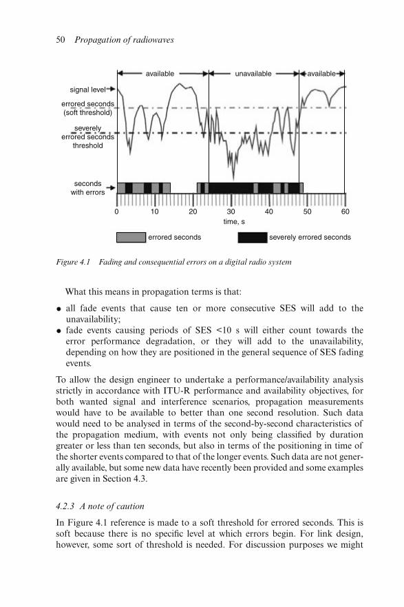
What this means in propagation terms is that:
• all fade events that cause ten or more consecutive SES will add to theunavailability;
• fade events causing periods of SES <10 s will either count towards theerror performance degradation, or they will add to the unavailability,depending on how they are positioned in the general sequence of SES fadingevents.
To allow the design engineer to undertake a performance/availability analysisstrictly in accordance with ITU-R performance and availability objectives, forboth wanted signal and interference scenarios, propagation measurementswould have to be available to better than one second resolution. Such datawould need to be analysed in terms of the second-by-second characteristics ofthe propagation medium, with events not only being classified by durationgreater or less than ten seconds, but also in terms of the positioning in time ofthe shorter events compared to that of the longer events. Such data are not gener-ally available, but some new data have recently been provided and some examplesare given in Section 4.3.
4.2.3 A note of caution
In Figure 4.1 reference is made to a soft threshold for errored seconds. This issoft because there is no specific level at which errors begin. For link design,however, some sort of threshold is needed. For discussion purposes we might
Figure 4.1 Fading and consequential errors on a digital radio system
50 Propagation of radiowaves
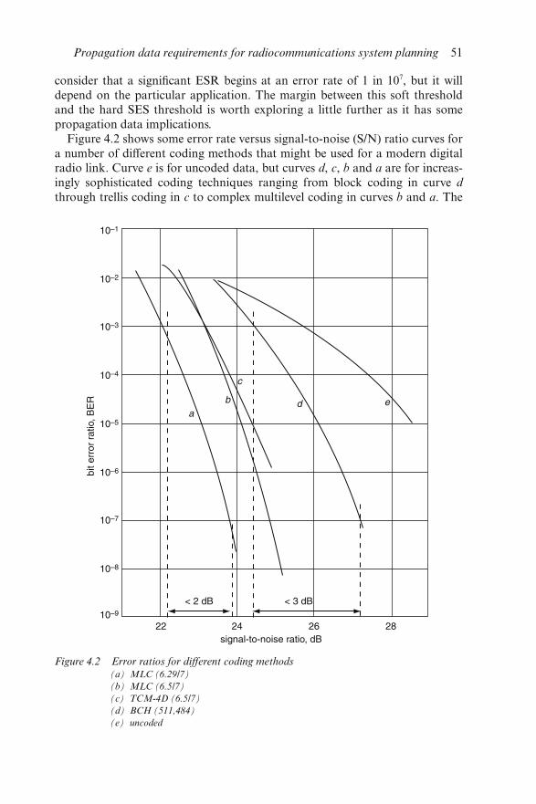
consider that a significant ESR begins at an error rate of 1 in 107, but it willdepend on the particular application. The margin between this soft thresholdand the hard SES threshold is worth exploring a little further as it has somepropagation data implications.
Figure 4.2 shows some error rate versus signal-to-noise (S/N) ratio curves fora number of different coding methods that might be used for a modern digitalradio link. Curve e is for uncoded data, but curves d, c, b and a are for increas-ingly sophisticated coding techniques ranging from block coding in curve d
through trellis coding in c to complex multilevel coding in curves b and a. The
Figure 4.2 Error ratios for different coding methods(a) MLC (6.29/7)
(b) MLC (6.5/7)
(c) TCM-4D (6.5/7)
(d) BCH (511,484)
(e) uncoded
Propagation data requirements for radiocommunications system planning 51
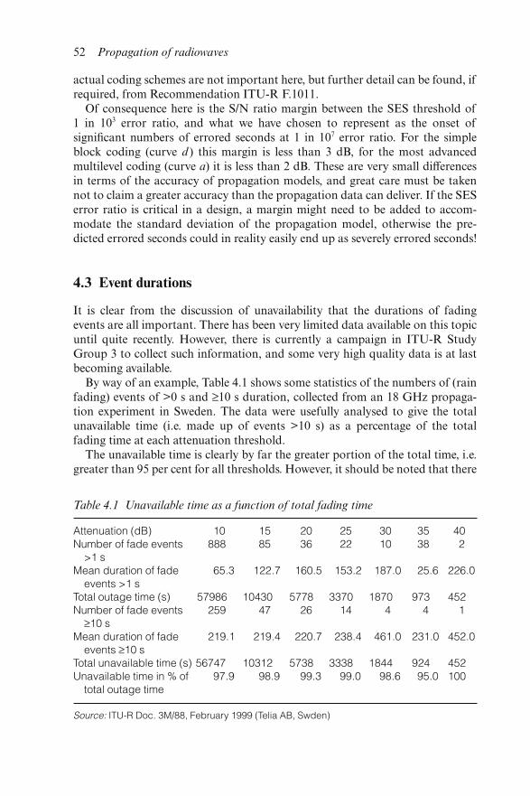
actual coding schemes are not important here, but further detail can be found, ifrequired, from Recommendation ITU-R F.1011.
Of consequence here is the S/N ratio margin between the SES threshold of1 in 103 error ratio, and what we have chosen to represent as the onset ofsignificant numbers of errored seconds at 1 in 107 error ratio. For the simpleblock coding (curve d ) this margin is less than 3 dB, for the most advancedmultilevel coding (curve a) it is less than 2 dB. These are very small differencesin terms of the accuracy of propagation models, and great care must be takennot to claim a greater accuracy than the propagation data can deliver. If the SESerror ratio is critical in a design, a margin might need to be added to accom-modate the standard deviation of the propagation model, otherwise the pre-dicted errored seconds could in reality easily end up as severely errored seconds!
4.3 Event durations
It is clear from the discussion of unavailability that the durations of fadingevents are all important. There has been very limited data available on this topicuntil quite recently. However, there is currently a campaign in ITU-R StudyGroup 3 to collect such information, and some very high quality data is at lastbecoming available.
By way of an example, Table 4.1 shows some statistics of the numbers of (rainfading) events of >0 s and ≥10 s duration, collected from an 18 GHz propaga-tion experiment in Sweden. The data were usefully analysed to give the totalunavailable time (i.e. made up of events >10 s) as a percentage of the totalfading time at each attenuation threshold.
The unavailable time is clearly by far the greater portion of the total time, i.e.greater than 95 per cent for all thresholds. However, it should be noted that there
Table 4.1 Unavailable time as a function of total fading time
Attenuation (dB) 10 15 20 25 30 35 40Number of fade events
>1 s888 85 36 22 10 38 2
Mean duration of fadeevents >1 s
65.3 122.7 160.5 153.2 187.0 25.6 226.0
Total outage time (s) 57986 10430 5778 3370 1870 973 452Number of fade events
≥10 s259 47 26 14 4 4 1
Mean duration of fadeevents ≥10 s
219.1 219.4 220.7 238.4 461.0 231.0 452.0
Total unavailable time (s) 56747 10312 5738 3338 1844 924 452Unavailable time in % of
total outage time97.9 98.9 99.3 99.0 98.6 95.0 100
Source: ITU-R Doc. 3M/88, February 1999 (Telia AB, Swden)
52 Propagation of radiowaves
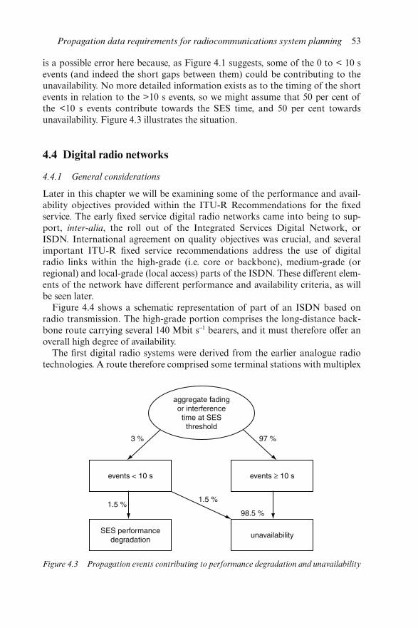
is a possible error here because, as Figure 4.1 suggests, some of the 0 to < 10 sevents (and indeed the short gaps between them) could be contributing to theunavailability. No more detailed information exists as to the timing of the shortevents in relation to the >10 s events, so we might assume that 50 per cent ofthe <10 s events contribute towards the SES time, and 50 per cent towardsunavailability. Figure 4.3 illustrates the situation.
4.4 Digital radio networks
4.4.1 General considerations
Later in this chapter we will be examining some of the performance and avail-ability objectives provided within the ITU-R Recommendations for the fixedservice. The early fixed service digital radio networks came into being to sup-port, inter-alia, the roll out of the Integrated Services Digital Network, orISDN. International agreement on quality objectives was crucial, and severalimportant ITU-R fixed service recommendations address the use of digitalradio links within the high-grade (i.e. core or backbone), medium-grade (orregional) and local-grade (local access) parts of the ISDN. These different elem-ents of the network have different performance and availability criteria, as willbe seen later.
Figure 4.4 shows a schematic representation of part of an ISDN based onradio transmission. The high-grade portion comprises the long-distance back-bone route carrying several 140 Mbit s−1 bearers, and it must therefore offer anoverall high degree of availability.
The first digital radio systems were derived from the earlier analogue radiotechnologies. A route therefore comprised some terminal stations with multiplex
Figure 4.3 Propagation events contributing to performance degradation and unavailability
Propagation data requirements for radiocommunications system planning 53
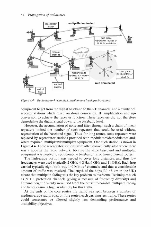
equipment to get from the digital baseband to the RF channels, and a number ofrepeater stations which relied on down conversion, IF amplification and up-conversion to achieve the repeater function. These repeaters did not thereforedemodulate the digital signal down to the baseband level.
However, the accumulation of noise and jitter through such a chain of linearrepeaters limited the number of such repeaters that could be used withoutregeneration of the baseband signal. Thus, for long routes, some repeaters werereplaced by regenerator stations provided with modulators/demodulators and,where required, multiplex/demultiplex equipment. One such station is shown inFigure 4.4. These regenerator stations were often conveniently sited where therewas a node in the radio network, because the same baseband and multiplexequipment was needed to split/combine baseband traffic from different routes.
The high-grade portion was needed to cover long distances, and thus lowfrequencies were used (typically 2 GHz, 4 GHz, 6 GHz and 11 GHz). Each hopcarried typically eight both-way 140 Mbit s−1 channels, and thus a considerableamount of traffic was involved. The length of the hops (30–45 km in the UK)meant that multipath fading was the key problem to overcome. Techniques suchas N + 1 protection channels (giving a measure of frequency diversity) andantenna height diversity were used from the outset to combat multipath fadingand hence ensure a high availability for this traffic.
At the ends of the core routes the traffic was split between a number ofmedium-grade radio, coax or fibre routes, each carrying less traffic. These routescould sometimes be allowed slightly less demanding performance andavailability objectives.
Figure 4.4 Radio network with high, medium and local grade sections
54 Propagation of radiowaves
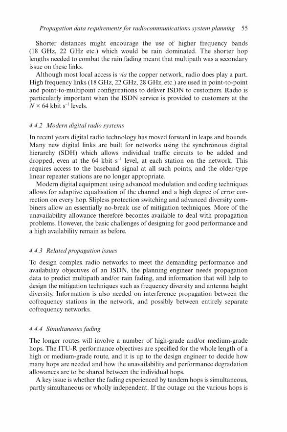
Shorter distances might encourage the use of higher frequency bands(18 GHz, 22 GHz etc.) which would be rain dominated. The shorter hoplengths needed to combat the rain fading meant that multipath was a secondaryissue on these links.
Although most local access is via the copper network, radio does play a part.High frequency links (18 GHz, 22 GHz, 28 GHz, etc.) are used in point-to-pointand point-to-multipoint configurations to deliver ISDN to customers. Radio isparticularly important when the ISDN service is provided to customers at theN × 64 kbit s−1 levels.
4.4.2 Modern digital radio systems
In recent years digital radio technology has moved forward in leaps and bounds.Many new digital links are built for networks using the synchronous digitalhierarchy (SDH) which allows individual traffic circuits to be added anddropped, even at the 64 kbit s−1 level, at each station on the network. Thisrequires access to the baseband signal at all such points, and the older-typelinear repeater stations are no longer appropriate.
Modern digital equipment using advanced modulation and coding techniquesallows for adaptive equalisation of the channel and a high degree of error cor-rection on every hop. Slipless protection switching and advanced diversity com-biners allow an essentially no-break use of mitigation techniques. More of theunavailability allowance therefore becomes available to deal with propagationproblems. However, the basic challenges of designing for good performance anda high availability remain as before.
4.4.3 Related propagation issues
To design complex radio networks to meet the demanding performance andavailability objectives of an ISDN, the planning engineer needs propagationdata to predict multipath and/or rain fading, and information that will help todesign the mitigation techniques such as frequency diversity and antenna heightdiversity. Information is also needed on interference propagation between thecofrequency stations in the network, and possibly between entirely separatecofrequency networks.
4.4.4 Simultaneous fading
The longer routes will involve a number of high-grade and/or medium-gradehops. The ITU-R performance objectives are specified for the whole length of ahigh or medium-grade route, and it is up to the design engineer to decide howmany hops are needed and how the unavailability and performance degradationallowances are to be shared between the individual hops.
A key issue is whether the fading experienced by tandem hops is simultaneous,partly simultaneous or wholly independent. If the outage on the various hops is
Propagation data requirements for radiocommunications system planning 55
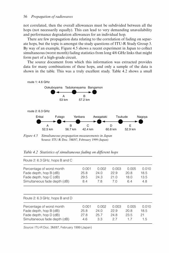
not correlated, then the overall allowances must be subdivided between all thehops (not necessarily equally). This can lead to very demanding unavailabilityand performance degradation allowances for an individual hop.
There are few propagation data relating to the correlation of fading on separ-ate hops, but the topic is amongst the study questions of ITU-R Study Group 3.By way of an example, Figure 4.5 shows a recent experiment in Japan to collectsimultaneous (worst month) fading statistics from long 4/6 GHz links that mightform part of a high-grade circuit.
The source document from which this information was extracted providesdata for many combinations of these hops, and only a sample of the data isshown in the table. This was a truly excellent study. Table 4.2 shows a small
Figure 4.5 Simultaneous propagation measurements in JapanSource: ITU-R Doc. 3M/87, February 1999 (Japan)
Table 4.2 Statistics of simultaneous fading on different hops
Route 2: 6.3 GHz, hops B and C
Percentage of worst month 0.001 0.002 0.003 0.005 0.010Fade depth, hop B (dB) 25.8 24.0 22.9 20.8 18.5Fade depth, hop C (dB) 29.5 24.3 21.0 18.0 13.5Simultaneous fade depth (dB) 8.4 7.8 7.0 6.4 4.8
Route 2: 6.3 GHz, hops B and D
Percentage of worst month 0.001 0.002 0.003 0.005 0.010Fade depth, hop B (dB) 25.8 24.0 22.9 20.8 18.5Fade depth, hop D (dB) 27.8 25.7 24.8 23.5 21Simultaneous fade depth (dB) 4.6 3.3 2.7 1.7 1.5
Source: ITU-R Doc. 3M/87, February 1999 (Japan)
56 Propagation of radiowaves
sample of the results from Route 2 of Figure 4.5. The upper part of the tableaddresses the simultaneous fading on hops B and C of Route 2, and the secondextract is for hops B and D. The data is shown for the high fading end of thedistributions, i.e. for time percentages from 0.001 per cent to 0.01 per cent.However, the data submitted to the ITU-R by Japan covers a much greater timepercentage range.
What is apparent from both these extracts is that, although all the hops sufferfading of up to about 30 dB for small time percentages, the levels of simul-taneous fading are quite small (8.4 dB maximum, even at 0.001 per cent of time).From these data one must conclude that all the significant fading (i.e. that likelyto cause errored seconds or severely errored seconds) is uncorrelated. This is badnews for the radio planner.
These data are for multipath fading. The limited work that has been done onrain fading on horizontally spaced or tandem paths shows broadly similar trends.
4.5 Long-term and short-term criteria
4.5.1 The long-term criteria
Customers for high-grade telecommunications services do not like errors.Indeed when the error rate is important, customers often keep their own regularcheck on the performance and availability of the circuits for which they arepaying. The challenge for radio networks has always been that coaxial cableand, more recently, optical fibre systems provide very high quality circuits, andfor radio to be a useful option for telecommunications networks, the samedemanding quality objectives have to be achieved.
Very short periods of errors due to propagation etc. are generally accepted,but regular errors under normal conditions are not. A margin must therefore beestablished above the noise level of the receiver such that the normal error rate isvery small indeed. This margin, together with the associated time percentage, isgenerally known as the long-term criterion.
The long-term performance requirements of modern digital telecommunica-tions circuits are very challenging indeed. Typically, for all but 10 or 20 per centof time, the expectation for fixed service links is an error rate of 1 in 1011 undernormal conditions. This represents one errored second in about 434 hours at the64 kbit s−1 level. This leaves little scope for accommodating adverse propagationeffects or interference problems.
Knowledge of the performance of the system hardware (e.g. the kind of datashown in Figure 4.2) allows the error performance and availability requirementsto be translated into equivalent carrier-to-noise or carrier-to-interference ratiorequirements.
For systems to achieve the required background error-rate performance, thedesign must provide a signal level that offers, for all but the stipulated timepercentage, an adequate margin to offset propagation fading and an assured
Propagation data requirements for radiocommunications system planning 57
margin over predictable interference levels from other stations in the networkand other spectrum users in the band. At around 10–20 per cent of time thepropagation and interference conditions are reasonably predictable, and areliable design can normally be achieved in this context.
4.5.2 The short-term criteria
For small percentages of time the propagation conditions and interference prob-lems will worsen. When the required signal fades too deeply (due, for instance, torain attenuation or multipath fading) and/or the incoming interference increasestoo much (perhaps due to ducting or hydrometeor scatter), the required systemwill eventually exceed a maximum permissible error rate (typically 1 in 103).When this occurs for periods longer than ten seconds, the system will be deemedto have become unavailable. Shorter periods of SES will affect the errorperformance. These situations must not be allowed to occur for more than astipulated percentage of time. The performance and availability objectives mustbe translated into short-term fade and interference margins which must beachieved by the system design for all but the acceptable percentages of time.
4.5.3 A simple design exercise
It is useful here to reflect on how the performance and availability requirementscan be matched to the available propagation data. This is a much-simplifiedexample, and it should not be taken as being the proper way to design aradio link. The first step is to convert the relevant error rates mentioned in theobjectives to the signal level margins which must exist above the noise and/orinterference levels.
As noted, to meet the errored seconds requirements it is necessary to keep thenominal signal at such a level above the background noise level that virtually noerrors occur for most of the time. This leaves the error allowances to be used upduring the short periods when the propagation conditions become more dif-ficult. The nominal (design) signal level should therefore equal or exceed thelevel required to achieve the necessary background error rate. The long-termthreshold A is shown associated with 20 per cent of time in Figure 4.6.
However, the signal will undoubtedly fade for some percentage of the time, asshown by the dashed line in Figure 4.6. Point B on this figure represents themargin, relative to the system noise floor (assuming a noise-limited situation), atwhich the system will produce an error rate of 1 in 103. If the signal falls beyondthis point severely errored seconds will occur and the hop could become unavail-able. The design received signal level must therefore be such that the predictedfading distribution passes through this level at, or below, the time percentageassociated with the short-term objective (in this case 0.01 per cent, purely chosenfor the purposes of illustration).
Furthermore, there may well be short periods of enhanced levels of interfer-ence, as illustrated by the predicted cumulative distribution for interference
58 Propagation of radiowaves
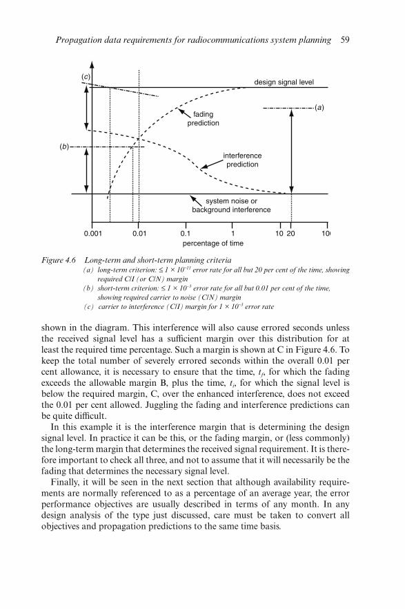
shown in the diagram. This interference will also cause errored seconds unlessthe received signal level has a sufficient margin over this distribution for atleast the required time percentage. Such a margin is shown at C in Figure 4.6. Tokeep the total number of severely errored seconds within the overall 0.01 percent allowance, it is necessary to ensure that the time, tf, for which the fadingexceeds the allowable margin B, plus the time, ti, for which the signal level isbelow the required margin, C, over the enhanced interference, does not exceedthe 0.01 per cent allowed. Juggling the fading and interference predictions canbe quite difficult.
In this example it is the interference margin that is determining the designsignal level. In practice it can be this, or the fading margin, or (less commonly)the long-term margin that determines the received signal requirement. It is there-fore important to check all three, and not to assume that it will necessarily be thefading that determines the necessary signal level.
Finally, it will be seen in the next section that although availability require-ments are normally referenced to as a percentage of an average year, the errorperformance objectives are usually described in terms of any month. In anydesign analysis of the type just discussed, care must be taken to convert allobjectives and propagation predictions to the same time basis.
Figure 4.6 Long-term and short-term planning criteria(a) long-term criterion: ≤ 1 × 10⁻¹¹ error rate for all but 20 per cent of the time, showing
required C/I (or C/N) margin
(b) short-term criterion: ≤ 1 × 10⁻³ error rate for all but 0.01 per cent of the time,
showing required carrier to noise (C/N) margin
(c) carrier to interference (C/I) margin for 1 × 10⁻³ error rate
Propagation data requirements for radiocommunications system planning 59
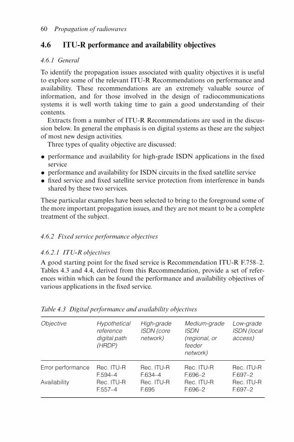
4.6 ITU-R performance and availability objectives
4.6.1 General
To identify the propagation issues associated with quality objectives it is usefulto explore some of the relevant ITU-R Recommendations on performance andavailability. These recommendations are an extremely valuable source ofinformation, and for those involved in the design of radiocommunicationssystems it is well worth taking time to gain a good understanding of theircontents.
Extracts from a number of ITU-R Recommendations are used in the discus-sion below. In general the emphasis is on digital systems as these are the subjectof most new design activities.
Three types of quality objective are discussed:
• performance and availability for high-grade ISDN applications in the fixedservice
• performance and availability for ISDN circuits in the fixed satellite service
• fixed service and fixed satellite service protection from interference in bandsshared by these two services.
These particular examples have been selected to bring to the foreground some ofthe more important propagation issues, and they are not meant to be a completetreatment of the subject.
4.6.2 Fixed service performance objectives
4.6.2.1 ITU-R objectives
A good starting point for the fixed service is Recommendation ITU-R F.758–2.Tables 4.3 and 4.4, derived from this Recommendation, provide a set of refer-ences within which can be found the performance and availability objectives ofvarious applications in the fixed service.
Table 4.3 Digital performance and availability objectives
Objective Hypotheticalreferencedigital path(HRDP)
High-gradeISDN (corenetwork)
Medium-gradeISDN(regional, orfeedernetwork)
Low-gradeISDN (localaccess)
Error performance Rec. ITU-RF.594–4
Rec. ITU-RF.634–4
Rec. ITU-RF.696–2
Rec. ITU-RF.697–2
Availability Rec. ITU-RF.557–4
Rec. ITU-RF.695
Rec. ITU-RF.696–2
Rec. ITU-RF.697–2
60 Propagation of radiowaves
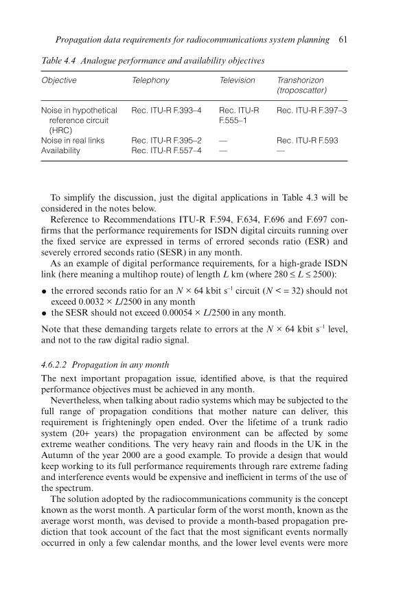
To simplify the discussion, just the digital applications in Table 4.3 will beconsidered in the notes below.
Reference to Recommendations ITU-R F.594, F.634, F.696 and F.697 con-firms that the performance requirements for ISDN digital circuits running overthe fixed service are expressed in terms of errored seconds ratio (ESR) andseverely errored seconds ratio (SESR) in any month.
As an example of digital performance requirements, for a high-grade ISDNlink (here meaning a multihop route) of length L km (where 280 ≤ L ≤ 2500):
• the errored seconds ratio for an N × 64 kbit s−1 circuit (N < = 32) should notexceed 0.0032 × L/2500 in any month
• the SESR should not exceed 0.00054 × L/2500 in any month.
Note that these demanding targets relate to errors at the N × 64 kbit s−1 level,and not to the raw digital radio signal.
4.6.2.2 Propagation in any month
The next important propagation issue, identified above, is that the requiredperformance objectives must be achieved in any month.
Nevertheless, when talking about radio systems which may be subjected to thefull range of propagation conditions that mother nature can deliver, thisrequirement is frighteningly open ended. Over the lifetime of a trunk radiosystem (20+ years) the propagation environment can be affected by someextreme weather conditions. The very heavy rain and floods in the UK in theAutumn of the year 2000 are a good example. To provide a design that wouldkeep working to its full performance requirements through rare extreme fadingand interference events would be expensive and inefficient in terms of the use ofthe spectrum.
The solution adopted by the radiocommunications community is the conceptknown as the worst month. A particular form of the worst month, known as theaverage worst month, was devised to provide a month-based propagation pre-diction that took account of the fact that the most significant events normallyoccurred in only a few calendar months, and the lower level events were more
Table 4.4 Analogue performance and availability objectives
Objective Telephony Television Transhorizon(troposcatter)
Noise in hypotheticalreference circuit(HRC)
Rec. ITU-R F.393–4 Rec. ITU-RF.555–1
Rec. ITU-R F.397–3
Noise in real links Rec. ITU-R F.395–2 — Rec. ITU-R F.593Availability Rec. ITU-R F.557–4 — —
Propagation data requirements for radiocommunications system planning 61
widely distributed through the year. The worst month is an important conceptand it is discussed more fully in Section 4.7.
4.6.2.3 Errored seconds ratio
The error performance objectives for the high-grade systems set out in Recom-mendation ITU-R F.634 (and indeed those for the medium-grade circuitsdescribed in Recommendation ITU-R F.696) specify both ESR and SESRtargets.
The SESR target is easiest to deal with as, via knowledge of the system hard-ware, it is possible to convert this to a defined attenuation threshold and adefined percentage of time.
The ESR target is more difficult, as it does not represent a fixed error rate, butrather a range of error rates from one per second up to 1 in 103. This translatesinto a range of attenuation values, with error rates increasing as the attenuationincreases, bounded at its upper limit by the SESR attenuation threshold. Todetermine the ESR performance, the predicted propagation distribution (forevents <10 s) would need to be convolved with the system fade/errorcharacteristics.
As the right kind of propagation information is not available, and as theanalysis would be complex, emphasis is generally placed on meeting the SESRobjective.
The errored seconds ratio is protected in another way. As just one error cancreate an ES, system designers try to keep the normal signal level well above thebackground noise and interference, i.e. the general design goal is virtually noerrors at all for most of the time. This leaves all of the ESR for the periods ofshort-term fading or interference. Having no errors is unrealistic, so a low errorrate (typically 1 in 1011 for terrestrial links and 1 in 107 for satellite links) is set asa long-term objective, i.e. for all but 10 or 20 per cent of time.
4.6.3 Fixed service availability objectives
4.6.3.1 ITU-R objectives
For digital systems, Recommendation 3 of Recommendation ITU-R F.557–4defines unavailability (of a both-way circuit) as ‘. . . at least 10 consecutiveseverely errored seconds (SES) in at least one direction of transmission’. Theunavailable time for the both-way circuit is therefore, theoretically, the combin-ation of the unavailable time for each direction of transmission, concurrentoutage in the two directions only counting once.
Reference to Recommendation ITU-R F.695 shows the availability objectiveA per cent for a high-grade ISDN link of length L km to be:
A = 100 − (0.3 × L/2500) %
This is 99.7 per cent of the time for the 2500 km route.However, what constitutes the time in this context remains, rather surpris-
62 Propagation of radiowaves
ingly, open to debate. Recommendation 1 of Recommendation 557 states ‘. . .the percentage being considered over a period of time sufficiently long to bestatistically valid, this period is probably greater than 1 year; the period of timeis under study . . .’.
On the assumption that the time in this case can be interpreted as an averageyear, then for a 300 km route, the value of A will be 99.976 per cent (an unavail-ability of only ∼7568 seconds).
Recommendation ITU-R F.696 shows that for medium-grade ISDN circuitsthere are four classes of system and that the unavailability in these cases is notdistance dependent and ranges from 0.033 to 0.1 per cent of time. Again,these represent time percentages of ‘. . . a period probably greater than oneyear . . .’.
Recommendation ITU-R F.697 shows that for local-grade ISDN circuits ‘theunavailability might range from 0.01% averaged over 1 year to up to 1.0%averaged over one or more years for a bi-directional radio system’.
There is clearly no single consistent definition of the base-line time for fixedservice availability, even after they have been in use for more than 30 years!
4.6.3.2 Propagation issues
The performance objectives discussed above were specified in the context of anymonth. Here we have a different requirement for propagation data relating to anaverage year.
The lack of clarity over the base-line time period to which the availabilityobjectives must be referenced is surprising. However, propagation predictionmodels are generally based, one way or another, on measured data, and the mostreliable data is that collected over a number of years in order to get a representa-tive average year. The pragmatic solution offered by the propagation communityis therefore the use of average year (otherwise known as average annual)statistics.
The ISDN performance and availability objectives generally apply to a wholehigh-grade (core network) route or a whole medium-grade (regional) route.These error performance and availability objectives cannot therefore be directlyapplied to a single hop on a route. The allowances for a single hop are generallysmaller.
Given that the unavailability also has to be apportioned between a number ofcauses, it becomes quite a complex task to determine the propagation fadingallowances for a particular hop, as they depend on the mitigation techniquesavailable (e.g. antenna height diversity, protection channels, error correction) onthe system to combat the effects of propagation fading and interference.
4.6.4 Fixed satellite service performance objectives
4.6.4.1 ITU-R objectives
It is possible to look at the comparable situation for the fixed satellite service,
Propagation data requirements for radiocommunications system planning 63
which generally provides high quality circuits over earth–space propagationpaths.
The ITU-R S. Series of Recommendations provides a set of texts dealing withthe performance and availability objectives for the fixed satellite service (FSS).Because of the particular nature of satellite circuits, and their heavy dependenceon coding, the FSS quality-of-service requirements tend to be more complexthan their fixed service counterparts.
With respect to the requirements for protecting FSS performance objectives,we can look to Recommendations ITU-R S.614-3 and S.1062-1.
For example, Recommendation ITU-R S.614 provides the allowable errorperformance for an HRDP in the fixed satellite service operating below 15 GHzwhen forming part of an international ISDN connection.
Recommendation 1 of Recommendation 614 states that: ‘The bit error ratio(BER) at the output (i.e. at either end of a two-way connection) of a satelliteHRDP operating below 15 GHz and forming part of a 64 kbit s−1 ISDNconnection should not exceed during the available time the values given below:
• 1 × 10⁻⁷ for more than 10 per cent of any month,
• 1 × 10⁻⁶ for more than 2 per cent of any month,
• 1 × 10⁻³ for more than 0.03 per cent of any month’.
In the case of this FSS ISDN application, the long-term error rate is specifiedas 1 in 107 at ten per cent of any month. In the FSS the link power budget has tobe tightly managed, and it is not possible to have a more generous backgrounderror rate. Furthermore, Note 11 of this Recommendation ventures into propa-gation advice when it states: ‘It is desirable that systems be planned on the basisof propagation data covering a period of at least 4 years. The performancerecommended to be met for any month should be based on the propagation datacorresponding to the median worst month of the year taken from the monthlystatistics of all the years for which reliable data are available’.
4.6.4.2 Propagation issues
As for the fixed service, the performance requirements of this example areexpressed in terms of a percentage of any month. What is different in this case isthat, instead of just long-term and short-term requirements, the performanceobjectives are described by a three-point distribution, with error-rate values forten, two, and 0.03 per cent of any month. In this case the propagation modelswould need to be able to provide fading and/or interference data for these vari-ous time percentages. It is therefore important that, to be of maximum use toplanning engineers now and in the future, propagation models can predict apropagation loss value for any time percentage likely to be needed. However, therealistic lower limit for average year statistics is about 0.0001 per cent (5.6 min-utes a year), although confidence falls much below 0.001 per cent unless datafrom an exceptionally long measurement period is available.
64 Propagation of radiowaves
4.6.5 Fixed satellite service availability objectives
4.6.5.1 ITU-R objectives
Recommendation ITU-R S.579-4 discusses the availability objectives for ahypothetical reference circuit (HRC) or hypothetical reference digital path(HRDP) when used in the FSS for PCM telephony, or as part of an ISDN.
Within this recommendation, Recommendation 3 states that: ‘the unavail-ability due to propagation should not be more than:
• 0.2 per cent of any month for one direction of an HRDP in the FSS
• 0.1 per cent of any year . . . for one direction of an HRC in the FSS’.
4.6.5.2 Propagation issues
In this case the availability requirement for digital circuits (the HRDP) isexpressed as a percentage of any month, and for the analogue case (the HRC)the requirement is based on any year. This is yet another descriptor of the base-line time which, if taken literally, would require the design engineer to addressthe most extreme years likely to be encountered over the planned lifetime of thesystem. However, pragmatism again comes into play, and for practical purposesit is taken to mean an average year.
4.6.6 Sharing between the fixed service and the fixed satellite service
As well as looking at the wanted signal performance and availability, it is usefulto look at the requirements for interference between fixed service and fixedsatellite service systems sharing the same frequency bands. Many of the mostimportant telecommunications bands are shared in this way.
When the performance and availability objectives for individual services aretranslated into sharing criteria the situation becomes more complex. ITU-RRecommendations in the SF Series apply here. For example, RecommendationITU-R SF.558-2 recommends maximum allowable values of interference fromterrestrial radio links to satellite systems employing 8-bit PCM encoded teleph-ony. To complement this, Recommendation ITU-R SF.615-1 gives maximumallowable values of interference from the fixed satellite service into terrestrialradio relay systems which may form part of an ISDN.
4.6.6.1 Fixed satellite service protection
For the protection of the fixed satellite service, Recommendation ITU-R SF.558makes the following recommendations:
• the interfering power, averaged over any ten minutes, should not exceed, formore than 20 per cent of any month, 10 per cent of the total noise powerat the input of the demodulator that would give rise to an error ratio of 1 in106;
Propagation data requirements for radiocommunications system planning 65
• the interfering RF power should not cause an increase of more than 0.03 percent of any month during which the bit error ratio exceeds 1 × 10⁻⁴ averagedover one minute;
• the interfering RF power should not cause an increase of more than 0.005 percent of any month during which the bit error ratio exceeds 1 × 10⁻³ averagedover one second.
These three protection criteria for the fixed satellite service protect both long-term and short-term error rate objectives, and all are clearly addressed in termsof any month.
4.6.6.2 Fixed service protection
For the protection of the fixed service, Recommendation ITU-R SF.615provides three equivalent criteria:
• the interfering emissions should not degrade the performance by causing anincrease of more than 0.0054 per cent of the period of time in any monthduring which the bit error ratio exceeds 1 × 10⁻³ (integration time onesecond);
• the interference emissions should not degrade the availability by causingan increase in the period of unavailability, as defined in RecommendationITU-R F.557, of more than 0.03 per cent of any year;
• the interference emissions should not degrade the performance by causing anincrease in the number of errored seconds measured at the 64 kbit s−1 interfaceby more than 0.032 per cent in any month.
In this case there are both worst-month performance and worst-monthavailability criteria to be met, together with an average year unavailabilityrequirement.
There is an apparent conflict between these recommendations and those forthe specific services discussed in Sections 4.6.3 and 4.6.4. The service-specificrecommendations (e.g. Recommendations F.557 and F.695) imply that the avail-ability objective should cover ‘. . . all causes that are statistically predictable . . .’,normally deemed to include propagation, interference and hardware failures(including restoration time). However, the recommendations discussed in thissection talk about not increasing the unavailability ‘. . . as defined in Recom-mendation ITU-R F.557 . . .’ by more than a given amount due to interferencearising from the sharing situation. This inconsistency is not helpful as it signifi-cantly affects the time percentages to be used for the interference prediction.
4.6.6.3 Propagation issues
For the protection of the fixed satellite service, Recommendation ITU-R SF.558introduces an additional requirement to those encountered in the examplesabove, i.e. that of specifying an integration time of longer than one second (e.g.ten minutes and one minute) for the counting of errors due to interference.
66 Propagation of radiowaves
To facilitate the evaluation of the interference environment for the satelliteservice the design engineer would ideally like to have available propagation datatailored to these integration times. Although interference propagation mechan-isms like ducting tend to have a relatively slow rate of change, there are manyothers (e.g. layer reflections, hydrometeor scatter and tropospheric scatter) thatcan be far more peaky in their behaviour. In some cases averaging over a minuteor ten minutes would make a significant difference compared to a one secondintegration time.
Unfortunately propagation models that can deal with different integrationtime requirements are not generally available, and it is difficult to see how suchcomplex performance requirements can be realistically fulfilled.
4.7 Worst month
4.7.1 The concept of the worst month
The need to design a radiocommunications system to meet performance andavailability objectives in any month is a tall order. Propagation conditions varyconsiderably from month to month, and the monthly variability can changesignificantly from year to year. Furthermore, it is not possible to be certainabout what might happen in any monthly period for the next 20 years or more,as it could be more extreme than anything so far observed. In order to providepropagation data to help the designer who is faced with quality objectives basedon any month, it was necessary to get away from this totally open-endedconcept. To provide a solution the propagation community came up with theconcept of the worst month, as defined in Recommendation ITU-R P.581-2.
The worst-month concept is only relevant to the higher-grade tele-communications services. It does not generally find applications in, for example,broadcasting, radio astronomy, space research, radio navigation or radiodetermination services, and arguably does not apply to terrestrial mobile orsatellite mobile telecommunications services which generally have more relaxedperformance and availability objectives than their fixed counterparts. In thecontext of interference assessment, worst month might only apply to some shar-ing scenarios and even then might only apply in one direction of interferencepropagation when only one of the sharing services required worst-monthprotection.
Worst-month propagation data has to be determined from extended meas-urement periods to ensure that a representative monthly variability is observed,particularly for the tails of the propagation distributions.
The propagation worst month concentrates on calendar months. Once severalyears of data are available, the data for the individual calendar months fromeach year (e.g. all the individual January data sets) can be averaged. The long-termaveraged data for each of the 12 calendar months can then be plotted togetherand the envelope of this set of monthly distributions provides the worst-month
Propagation data requirements for radiocommunications system planning 67
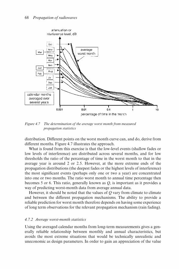
distribution. Different points on the worst month curve can, and do, derive fromdifferent months. Figure 4.7 illustrates the approach.
What is found from this exercise is that the low-level events (shallow fades orlow levels of interference) are distributed across several months, and for lowthresholds the ratio of the percentage of time in the worst month to that in theaverage year is around 2 or 2.5. However, at the more extreme ends of thepropagation distributions (the deepest fades or the highest levels of interference)the most significant events (perhaps only one or two a year) are concentratedinto one or two months. The ratio worst month to annual time percentage thenbecomes 5 or 6. This ratio, generally known as Q, is important as it provides away of predicting worst-month data from average annual data.
However, it should be noted that the values of Q vary from climate to climateand between the different propagation mechanisms. The ability to provide areliable prediction for worst month therefore depends on having some experienceof long term observations for the relevant propagation mechanism (rain fading).
4.7.2 Average worst-month statistics
Using the averaged calendar months from long-term measurements gives a gen-erally reliable relationship between monthly and annual characteristics, butavoids the most extreme situations that would be technically unrealistic anduneconomic as design parameters. In order to gain an appreciation of the value
Figure 4.7 The determination of the average worst month from measured
propagation statistics
68 Propagation of radiowaves
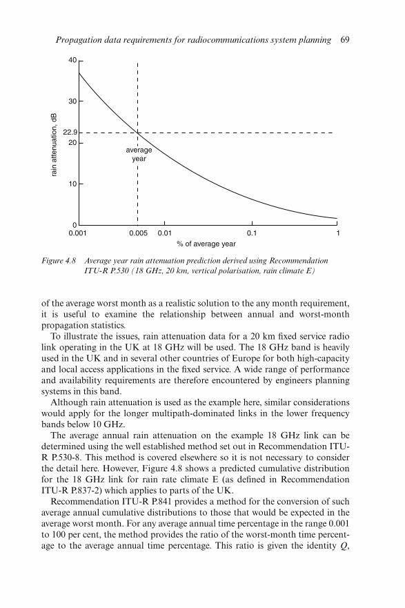
of the average worst month as a realistic solution to the any month requirement,it is useful to examine the relationship between annual and worst-monthpropagation statistics.
To illustrate the issues, rain attenuation data for a 20 km fixed service radiolink operating in the UK at 18 GHz will be used. The 18 GHz band is heavilyused in the UK and in several other countries of Europe for both high-capacityand local access applications in the fixed service. A wide range of performanceand availability requirements are therefore encountered by engineers planningsystems in this band.
Although rain attenuation is used as the example here, similar considerationswould apply for the longer multipath-dominated links in the lower frequencybands below 10 GHz.
The average annual rain attenuation on the example 18 GHz link can bedetermined using the well established method set out in Recommendation ITU-R P.530-8. This method is covered elsewhere so it is not necessary to considerthe detail here. However, Figure 4.8 shows a predicted cumulative distributionfor the 18 GHz link for rain rate climate E (as defined in RecommendationITU-R P.837-2) which applies to parts of the UK.
Recommendation ITU-R P.841 provides a method for the conversion of suchaverage annual cumulative distributions to those that would be expected in theaverage worst month. For any average annual time percentage in the range 0.001to 100 per cent, the method provides the ratio of the worst-month time percent-age to the average annual time percentage. This ratio is given the identity Q,
Figure 4.8 Average year rain attenuation prediction derived using Recommendation
ITU-R P.530 (18 GHz, 20 km, vertical polarisation, rain climate E)
Propagation data requirements for radiocommunications system planning 69
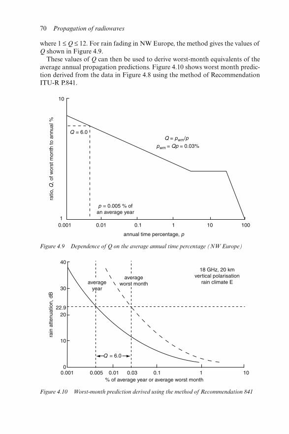
where 1 ≤ Q ≤ 12. For rain fading in NW Europe, the method gives the values ofQ shown in Figure 4.9.
These values of Q can then be used to derive worst-month equivalents of theaverage annual propagation predictions. Figure 4.10 shows worst month predic-tion derived from the data in Figure 4.8 using the method of RecommendationITU-R P.841.
Figure 4.9 Dependence of Q on the average annual time percentage (NW Europe)
Figure 4.10 Worst-month prediction derived using the method of Recommendation 841
70 Propagation of radiowaves
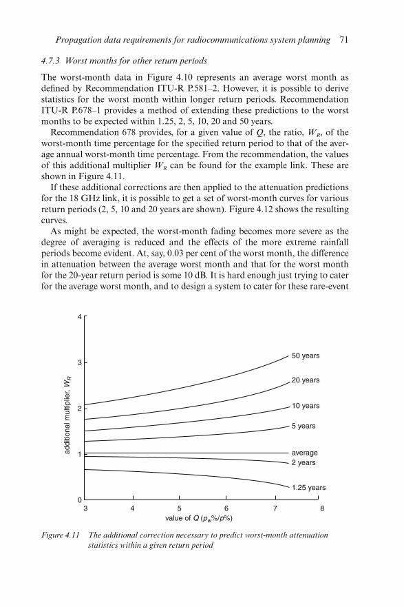
4.7.3 Worst months for other return periods
The worst-month data in Figure 4.10 represents an average worst month asdefined by Recommendation ITU-R P.581–2. However, it is possible to derivestatistics for the worst month within longer return periods. RecommendationITU-R P.678–1 provides a method of extending these predictions to the worstmonths to be expected within 1.25, 2, 5, 10, 20 and 50 years.
Recommendation 678 provides, for a given value of Q, the ratio, WR, of theworst-month time percentage for the specified return period to that of the aver-age annual worst-month time percentage. From the recommendation, the valuesof this additional multiplier WR can be found for the example link. These areshown in Figure 4.11.
If these additional corrections are then applied to the attenuation predictionsfor the 18 GHz link, it is possible to get a set of worst-month curves for variousreturn periods (2, 5, 10 and 20 years are shown). Figure 4.12 shows the resultingcurves.
As might be expected, the worst-month fading becomes more severe as thedegree of averaging is reduced and the effects of the more extreme rainfallperiods become evident. At, say, 0.03 per cent of the worst month, the differencein attenuation between the average worst month and that for the worst monthfor the 20-year return period is some 10 dB. It is hard enough just trying to caterfor the average worst month, and to design a system to cater for these rare-event
Figure 4.11 The additional correction necessary to predict worst-month attenuation
statistics within a given return period
Propagation data requirements for radiocommunications system planning 71
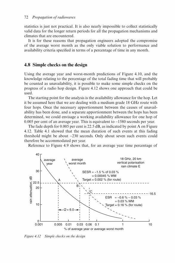
statistics is just not practical. It is also nearly impossible to collect statisticallyvalid data for the longer return periods for all the propagation mechanisms andclimates that are encountered.
It is for these reasons that propagation engineers adopted the compromiseof the average worst month as the only viable solution to performance andavailability criteria specified in terms of a percentage of time in any month.
4.8 Simple checks on the design
Using the average year and worst-month predictions of Figure 4.10, and theknowledge relating to the percentage of the total fading time that will probablybe counted as unavailability, it is possible to make some simple checks on theprogress of a radio hop design. Figure 4.12 shows one approach that could beused.
The starting point for the analysis is the availability allowance for the hop. Letit be assumed here that we are dealing with a medium grade 18 GHz route withfour hops. Once the necessary apportionment between the causes of unavail-ability has been done, and a separate apportionment between the hops has beendetermined, we could envisage a working availability allowance for one hop of0.005 per cent of an average year. This is equivalent to ∼1580 seconds per year.
The fade depth for 0.005 per cent is 22.5 dB, as indicated by point A on Figure4.12. Table 4.1 showed that the mean duration of such events at this fadingthreshold might be about ∼230 seconds. Only about seven such events couldtherefore be accommodated per year.
Reference to Figure 4.9 shows that, for an average year time percentage of
Figure 4.12 Simple checks on the design
72 Propagation of radiowaves
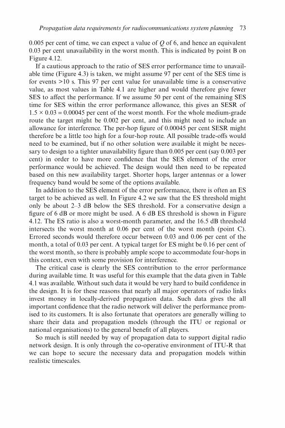
0.005 per cent of time, we can expect a value of Q of 6, and hence an equivalent0.03 per cent unavailability in the worst month. This is indicated by point B onFigure 4.12.
If a cautious approach to the ratio of SES error performance time to unavail-able time (Figure 4.3) is taken, we might assume 97 per cent of the SES time isfor events >10 s. This 97 per cent value for unavailable time is a conservativevalue, as most values in Table 4.1 are higher and would therefore give fewerSES to affect the performance. If we assume 50 per cent of the remaining SEStime for SES within the error performance allowance, this gives an SESR of1.5 × 0.03 = 0.00045 per cent of the worst month. For the whole medium-graderoute the target might be 0.002 per cent, and this might need to include anallowance for interference. The per-hop figure of 0.00045 per cent SESR mighttherefore be a little too high for a four-hop route. All possible trade-offs wouldneed to be examined, but if no other solution were available it might be neces-sary to design to a tighter unavailability figure than 0.005 per cent (say 0.003 percent) in order to have more confidence that the SES element of the errorperformance would be achieved. The design would then need to be repeatedbased on this new availability target. Shorter hops, larger antennas or a lowerfrequency band would be some of the options available.
In addition to the SES element of the error performance, there is often an EStarget to be achieved as well. In Figure 4.2 we saw that the ES threshold mightonly be about 2–3 dB below the SES threshold. For a conservative design afigure of 6 dB or more might be used. A 6 dB ES threshold is shown in Figure4.12. The ES ratio is also a worst-month parameter, and the 16.5 dB thresholdintersects the worst month at 0.06 per cent of the worst month (point C).Errored seconds would therefore occur between 0.03 and 0.06 per cent of themonth, a total of 0.03 per cent. A typical target for ES might be 0.16 per cent ofthe worst month, so there is probably ample scope to accommodate four-hops inthis context, even with some provision for interference.
The critical case is clearly the SES contribution to the error performanceduring available time. It was useful for this example that the data given in Table4.1 was available. Without such data it would be very hard to build confidence inthe design. It is for these reasons that nearly all major operators of radio linksinvest money in locally-derived propagation data. Such data gives the allimportant confidence that the radio network will deliver the performance prom-ised to its customers. It is also fortunate that operators are generally willing toshare their data and propagation models (through the ITU or regional ornational organisations) to the general benefit of all players.
So much is still needed by way of propagation data to support digital radionetwork design. It is only through the co-operative environment of ITU-R thatwe can hope to secure the necessary data and propagation models withinrealistic timescales.
Propagation data requirements for radiocommunications system planning 73

Chapter 5
Electromagnetic wave propagation
M.J. Mehler
5.1 Introduction
The objective of this Chapter is to introduce the principles of electromagnetictheory which are essential to an understanding of radiowave propagation.Where possible a practical engineering approach has been adopted. However,the material has been structured to provide those with a more mathematicalbackground with a satisfactory account of the subject, together with referencesto further reading material.
Initially, propagation between two antennas in free space is considered bymeans of power flux concepts. This enables important ideas such as free-spacepath loss, antenna gain and effective aperture to be introduced. Maxwell’s equa-tions are presented. and plane-wave solutions are derived as a means of intro-ducing polarisation, wave impedance and electromagnetic power flow. Finally,radiation from a current distribution is examined and illustrated by deriving thefields of a dipole antenna.
5.2 Power budget
Radio propagation engineers are often concerned with determining the powerreceived by a distant antenna when the transmitted power is given. Such acalculation is the key to the design of radio systems and involves the determin-ation of the power budget taking account of each element of the radio link. Inpractice, when both transmitter and receiver are in free space, this calculationcan easily be made using a simple conservation-of-energy argument. Moreover,even when the antennas are not in free space the concept of a link budget, basedon energy conservation, can be extended to take account of effects such asdiffraction loss.
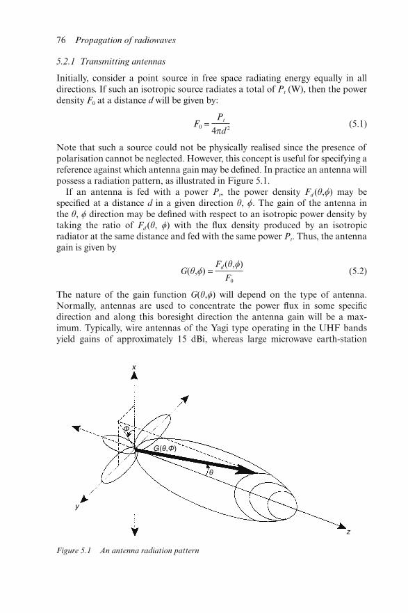
5.2.1 Transmitting antennas
Initially, consider a point source in free space radiating energy equally in alldirections. If such an isotropic source radiates a total of Pt (W), then the powerdensity F0 at a distance d will be given by:
F0 = Pt
4πd 2(5.1)
Note that such a source could not be physically realised since the presence ofpolarisation cannot be neglected. However, this concept is useful for specifying areference against which antenna gain may be defined. In practice an antenna willpossess a radiation pattern, as illustrated in Figure 5.1.
If an antenna is fed with a power Pt, the power density Fd (θ,) may bespecified at a distance d in a given direction θ, . The gain of the antenna inthe θ, direction may be defined with respect to an isotropic power density bytaking the ratio of Fd (θ, ) with the flux density produced by an isotropicradiator at the same distance and fed with the same power Pt. Thus, the antennagain is given by
G(θ,) = Fd (θ,)
F0
(5.2)
The nature of the gain function G(θ,) will depend on the type of antenna.Normally, antennas are used to concentrate the power flux in some specificdirection and along this boresight direction the antenna gain will be a max-imum. Typically, wire antennas of the Yagi type operating in the UHF bandsyield gains of approximately 15 dBi, whereas large microwave earth-station
Figure 5.1 An antenna radiation pattern
76 Propagation of radiowaves
antennas of about 3 m diameter can produce gains in the order of 50 dBi. Herethe i denotes the gain with respect to that of an isotropic antenna.
5.2.2 Receiving antennas
The power density at a distance d in a given direction from a transmittingantenna is Fd(θ,). A useful expression for this quantity can be found bycombining Eqns 5.1 and 5.2, to yield:
Fd(θ,) = PtGt(θ,)
4πd 2(5.3)
where Gt, is the gain of the transmitting antenna. A receiving antenna placed inthis power flux will deliver a power Pr into a load connected to the antennaterminals or waveguide port. To facilitate the calculation of Pr we may considerthe antenna to be presenting an effective collecting-aperture area Ae, to theincoming field. Hence, the received power becomes:
Pr = PtGt(θ,)Ae
4πd 2(5.4)
The concept of an effective aperture area is easily interpreted for reflectorantennas, where a paraboloid of diameter D presents a projected area πD2/4 to anormally incident wave. Even if ohmic losses in the antenna are neglected, someof the incident field will be reflected and hence not all of the incident energy willbe absorbed in the antenna load. If the paraboloid is rotated, the incident wavewill no longer be normal to the aperture. Hence, additional incident energy willbe reflected and thus the received power in the load will be further reduced in amanner consistent with the antenna pattern. These considerations illustrate thatthe effective aperture area of an antenna is not necessarily equal to the physicalarea A = πD2/4. Moreover, the effective area will depend on the direction of theincident field. It is possible to relate the effective aperture to the antenna gainthrough the relation:
Ae(θ,) = G(θ,)λ2
4π(5.5)
The ratio between the effective aperture and the physical area, in the directionof maximum gain, is a measure of antenna efficiency η, so that η = Ae /A.Combining this definition with Eqn. 5.5 yields a useful expression for themaximum antenna gain, namely:
G = �πD
λ �2
η (5.6)
Although the above discussion has been concerned with reflector antennas, theconcept of effective aperture area is also commonly applied to wire antennas.
Electromagnetic wave propagation 77
5.2.3 Free-space transmission loss
Combining Eqn. 5.4 with Eqn. 5.5 permits the received power to be written interms of the transmitting and receiving antenna gains Gt, and Gr, respectively.The resulting expression takes the form:
Pr = PtGtGr� λ
4πD�2
(5.7)
To interpret this result, note that if both transmitting and receiving antennaspossess a gain of unity, then in free space the ratio Pr/Pt depends on (λ/4πD)2,which is simply the free-space loss.
5.2.4 Link power budget
Radio engineers usually express Eqn. 5.7 in decibels, so that we may write:
Pr(dBw) = Pt(dBw) + Gt(dBi) + Gr(dBi) − Lbf (dB) (5.8)
where:
Lbf = 20{log10(4πd) − log10(λ)}
noting that λ = c/f (c is the velocity of light in a vacuum = 3 × 10⁸ ms−1) andtaking f to be in MHz and d in km, the following standard result is obtained:
Lbf = 32.44 + 20log10 f + 20log10d (5.9)
(Note that dBw is with respect to 1 W; dBi is the gain with respect to an isotropicantenna.)
Eqn. 5.8 can be extended to treat propagation between antennas which are notin free space by making allowance for additional sources of path loss. Forexample, propagation over a path with terrain features introduces loss inaddition to that of free space. This additional diffraction loss, Ld, can easilybe included into the link budget, so that Eqn. 5.8 becomes
Pr = Pt + Gt + Gr − Lbf − Ld (5.10)
Clearly, this approach can be extended to include other loss mechanisms, such asantenna feeder losses. Eqn. 5.10 forms the basis of many radio-system-linkbudget calculations.
5.3 Basic electromagnetic theory
The above discussion has only been concerned with the use of conservation-of-energy arguments where the electromagnetic field has been treated as a scalarpower flux. In reality this model is inadequate and better agreement withexperimental observation is achieved by treating electromagnetic effects in termsof the interaction of charged particles with a vector field. For engineering
78 Propagation of radiowaves
applications it is often sufficient to describe these electromagnetic phenomenaby means of a classical field theory, namely Maxwell’s equations. These equa-tions relate the electric field E (V m−1) and the magnetic field H (A m−1) to thecurrent density J (A m−2) and the charge density ρ (C m−3).
They may be written in the form:
∇ × E = −μ ∂H∂t
(5.11a)
∇ × H = J + ε∂E∂t
(5.11b)
∇ . (εE) = ρ (5.11c)
∇ . (μH) = 0 (5.11d)
where ε and μ are the permittivity and permeability of the medium. They areoften written as ε = ε0 εr, and μ = μ0 μr, where μr = εr = 1 in free space, and ε0 =8.854 × 10¹² F m−1, μ0 = 4π × 10−7 H m−1.
Significant simplification of Maxwell’s equations can be achieved in freespace where both J and ρ are zero. Taking the curl of Eqn. 5.11a and using Eqn.5.11b to eliminate H gives:
∇ × ∇ × E = −μ0ε0
∂2E∂t2
(5.12)
This may be further simplified by means of a standard vector identity to give
−∇2E + ∇(∇ .E) = −μ0ε∂2E∂t2
(5.13)
Since in Eqn. 5.11c ρ = 0 and ε = ε0 (constant), Eqn. 5.13 may be furtherreduced to:
∇2E − μ0ε0
∂2E∂t2
= 0 (5.14)
This is the well known free-space wave equation for E.
5.3.1 Plane-wave solutions
In general, solutions to Eqn. 5.14 are difficult to obtain for many importantengineering problems. However, a number of very useful properties of the elec-tromagnetic field can be deduced by considering simple plane-wave solutions.The equation for a plane wave which is travelling in the positive z direction, withpolarisation in the x direction, may be written as:
E = E0 cos(ωt − kz)x (5.15)
where E0 is the amplitude of the wave, ω is the angular frequency 2πf and k the
Electromagnetic wave propagation 79
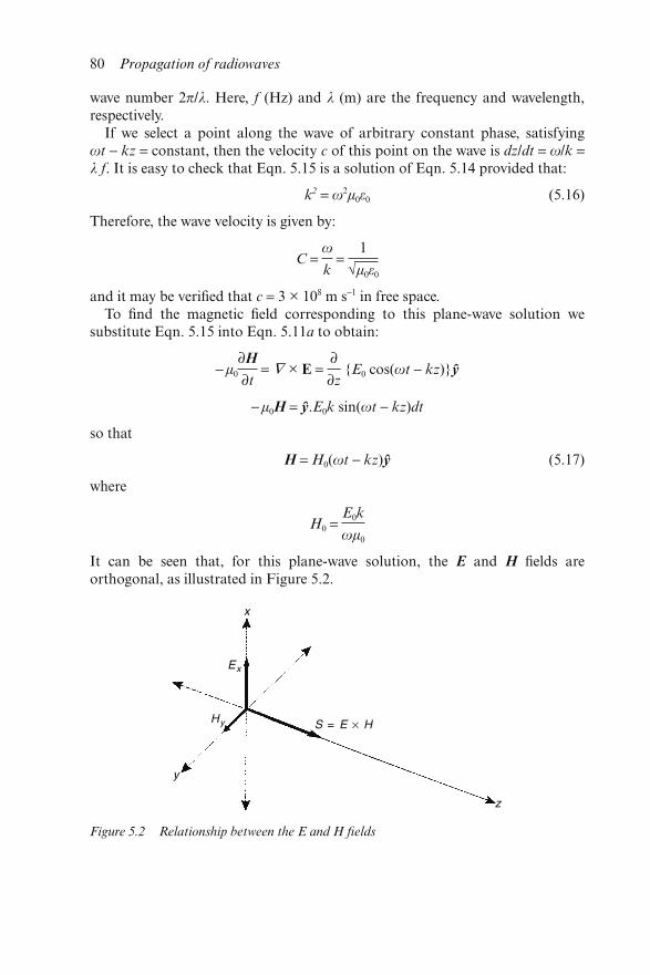
wave number 2π/λ. Here, f (Hz) and λ (m) are the frequency and wavelength,respectively.
If we select a point along the wave of arbitrary constant phase, satisfyingωt − kz = constant, then the velocity c of this point on the wave is dz/dt = ω/k =λ f. It is easy to check that Eqn. 5.15 is a solution of Eqn. 5.14 provided that:
k2 = ω2μ0ε0 (5.16)
Therefore, the wave velocity is given by:
C = ω
k =
1
√μ0ε0
and it may be verified that c = 3 × 10⁸ m s−1 in free space.To find the magnetic field corresponding to this plane-wave solution we
substitute Eqn. 5.15 into Eqn. 5.11a to obtain:
−μ0
∂H∂t
= ∇ × E = ∂∂z
{E0 cos(ωt − kz)}y
−μ0H = y.E0k sin(ωt − kz)dt
so that
H = H0(ωt − kz)y (5.17)
where
H0 = E0k
ωμ0
It can be seen that, for this plane-wave solution, the E and H fields areorthogonal, as illustrated in Figure 5.2.
Figure 5.2 Relationship between the E and H fields
80 Propagation of radiowaves
5.3.2 Wave impedance
It is evident that the ratio of the E- and H-field amplitudes in Eqn. 5.15 andEqn. 5.l7 is a constant, namely:
|E|
|H| =
Ex
Hy
= ωμ0
k = �μ0
ε0
(5.18)
This ratio is called the free-space wave impedance since it has units of ohms, andis usually denoted by Z0, which for this free-space case has an approximate valueof 377Ω. It is analogous to the ratio of voltage and current in an electric circuit.
5.3.3 Power flow and Poynting’s theorem
In the same way that the product of voltage and current may be used to calculatepower in an electric circuit, a vector product of E and H gives the power densityin the electromagnetic field. For the plane-wave solution, the power flow alongthe Z direction is (|E| |H|)/2 W m−2. Here the factor 1/2 in this expression has beenintroduced because E0 and H0 are peak values, whereas the power density is inroot mean square units. Using Eqns. 5.15 and 5.17, this expression reduces to:
E20
2z0
= Z0
2 H2
0
In general the E and H fields may not be orthogonal and in this case the aboveresult is not valid. However, it is possible to show that the power flow in anelectromagnetic field may be represented by the Poynting vector S [122], whichpoints in the direction of power flow and has a magnitude equal to the powerdensity, and is defined by:
S = E × H (5.19)
5.3.4 Exponential notation
Plane-wave solutions occur commonly in engineering problems. Indeed, it ispossible to represent arbitrary field distributions by a sum of plane waves ofvarying amplitude, phase and direction. It is also possible to simplify themanipulation of plane-wave expressions by introducing exponential notation,namely:
Re[exp{j(ωt − kz)}] = cos(ωt − kz) (5.20)
Hence, Eqn. 5.15 is written as:
E = E0 Re{exp(jωt)exp(−jkz)}x (5.21)
The exp(jωt) term is present because the field varies harmonically with time.Such steady-state solutions arise commonly in radio engineering problems. InMaxwell’s equations the adoption of the harmonic time dependence of Eqn.
Electromagnetic wave propagation 81
5.21 implies that differentiation with respect to time is replaced by jω, so thatEqns. 5.11a–d reduce to:
∇ × E = − jωμH (5.22a)
∇ × H = J + jωεE (5.22b)
∇ . εE = ρ (5.22c)
∇ .μH = 0 (5.22d)
The wave equation corresponding to Eqn. 5.14 follows by taking the curl ofEqn. 5.22a and using Eqn. 5.22b to eliminate H, and is given by:
∇ 2 E + k2 E = 0 (5.23)
It is easily shown that Eqn. 5.21 is a solution of Eqn. 5.23. Thus, using thisshorthand notation, Eqn. 5.21 becomes:
E = E0 exp(− jkz)x (5.24)
When interpreting this equation, or any solution of Eqn. 5.23, the need tomultiply by exp(− jkz) and take the real part should be borne in mind.
5.4 Radiation from current distributions
So far the plane-wave solutions considered have been obtained without anyreference to the current distribution which excites them. This is manifest by thearbitrary nature of E0 in Eqn. 5.15. In reality, E0 would be determined by thesource currents. More generally, if the field were represented by a superpositionof plane waves, known as a plane-wave spectrum, the amplitude, phase anddirection of each plane wave would be determined by the source-currentdistribution.
When calculating the field radiated by a current distribution, such as thatsupported on an antenna structure, it is often more convenient to work with avector potential, namely A. This potential may be introduced through thestandard result ∇.∇ × A = 0, and it may be deduced from Eqn. 5.11d that:
μH = ∇ × A (5.25)
Substituting Eqn. 5.25 into Eqns 5.11a–d yields a wave equation for A of theform:
∇ 2 A + k2 A = −μ0J (5.26)
If the current distribution is bounded by a volume v0, the field A in thefree-space region outside the volume v0 can be written explicitly in the form:
A(r) = μ
4π �J(r0)
exp(−jk|r − r0|)
|r − r0|dv0 (5.27)
82 Propagation of radiowaves
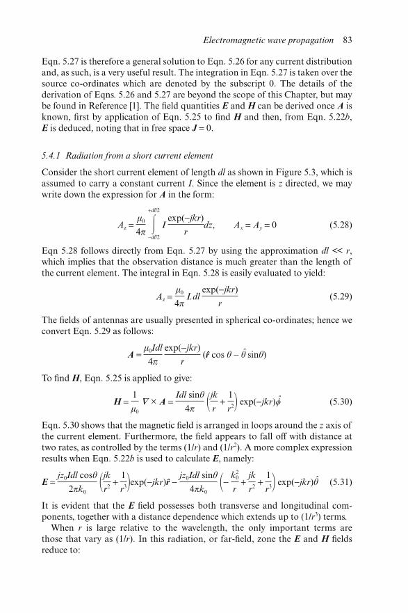
Eqn. 5.27 is therefore a general solution to Eqn. 5.26 for any current distributionand, as such, is a very useful result. The integration in Eqn. 5.27 is taken over thesource co-ordinates which are denoted by the subscript 0. The details of thederivation of Eqns. 5.26 and 5.27 are beyond the scope of this Chapter, but maybe found in Reference [1]. The field quantities E and H can be derived once A isknown, first by application of Eqn. 5.25 to find H and then, from Eqn. 5.22b,E is deduced, noting that in free space J = 0.
5.4.1 Radiation from a short current element
Consider the short current element of length dl as shown in Figure 5.3, which isassumed to carry a constant current I. Since the element is z directed, we maywrite down the expression for A in the form:
Az = μ0
4π �+dl/2
−dl/2
Iexp(−jkr)
rdz, Ax = Ay = 0 (5.28)
Eqn 5.28 follows directly from Eqn. 5.27 by using the approximation dl << r,which implies that the observation distance is much greater than the length ofthe current element. The integral in Eqn. 5.28 is easily evaluated to yield:
Az = μ0
4π I.dl
exp(−jkr)
r(5.29)
The fields of antennas are usually presented in spherical co-ordinates; hence weconvert Eqn. 5.29 as follows:
A = μ0Idl
4π
exp(−jkr)
r (r cos θ − θ sinθ)
To find H, Eqn. 5.25 is applied to give:
H = 1
μ0
∇ × A = Idl sinθ
4π �jkr +
1
r2� exp(−jkr) (5.30)
Eqn. 5.30 shows that the magnetic field is arranged in loops around the z axis ofthe current element. Furthermore, the field appears to fall off with distance attwo rates, as controlled by the terms (1/r) and (1/r2). A more complex expressionresults when Eqn. 5.22b is used to calculate E, namely:
E = jz0Idl cosθ
2πk0�jkr2
+ 1
r3�exp(−jkr)r − jz0Idl sinθ
4πk0
�− k2
0
r +
jk
r2 +
1
r3� exp(−jkr)θ (5.31)
It is evident that the E field possesses both transverse and longitudinal com-ponents, together with a distance dependence which extends up to (1/r3) terms.
When r is large relative to the wavelength, the only important terms arethose that vary as (1/r). In this radiation, or far-field, zone the E and H fieldsreduce to:
Electromagnetic wave propagation 83
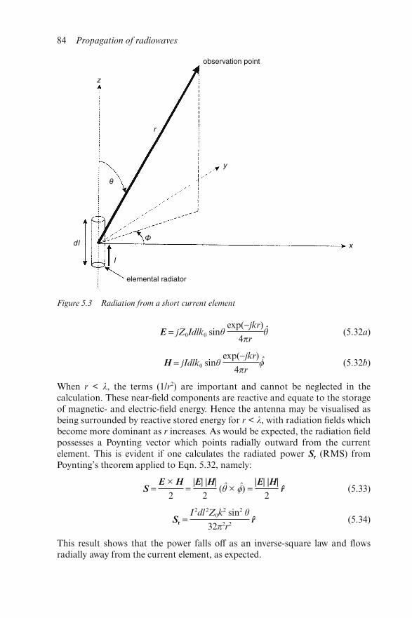
E = jZ0Idlk0 sinθ exp(−jkr)
4πrθ (5.32a)
H = jIdlk0 sinθ exp(−jkr)
4πr (5.32b)
When r < λ, the terms (1/r2) are important and cannot be neglected in thecalculation. These near-field components are reactive and equate to the storageof magnetic- and electric-field energy. Hence the antenna may be visualised asbeing surrounded by reactive stored energy for r < λ, with radiation fields whichbecome more dominant as r increases. As would be expected, the radiation fieldpossesses a Poynting vector which points radially outward from the currentelement. This is evident if one calculates the radiated power Sr (RMS) fromPoynting’s theorem applied to Eqn. 5.32, namely:
S = E × H
2 =
|E| |H|
2(θ × ) =
|E| |H|
2r (5.33)
Sr = I 2dl 2Z0k
2 sin2 θ
32π2r2r (5.34)
This result shows that the power falls off as an inverse-square law and flowsradially away from the current element, as expected.
Figure 5.3 Radiation from a short current element
84 Propagation of radiowaves
To calculate the total radiated power Pr it is necessary to integrate Eqn. 5.34over a complete sphere enclosing the current element, which yields the surfaceintegral:
Pr = I 2dl 2Z0k
2
32π2 �2π
0
�π
0
sin2θ
r2 (r2 sinθ)dθd
Integration over is straightforward, but to facilitate the integration over θ
the substitution u = cosθ is made, to yield:
Pr = I 2dl 2Z0k
2
16π �+1
−1
(1−u 2)du
which reduces to
Pr = I 2dl 2Z0k
2
12π(5.35)
5.4.2 Radiation resistance
If a source is connected to the antenna terminals and supplies a given power PR,we may regard the power as being supplied to an effective radiation resistanceRrad. Although this is not a physical resistance, it absorbs a power equal to thatbeing radiated in to the far field. Since I is a peak value, equating the powersupplied to Rrad to that which is radiated gives:
1
2 I 2Rrad =
I 2 dl 2Z0k2
12π
Therefore
Rrad = Z0(kdl)2
6π = 80π2 �dl
λ �2
(5.36)
As an example, at a frequency of 1 MHz (λ = 300 m) and with an antenna oflength dl = 1 m, Rrad = 0.0084 Ω. In practice it would be difficult to match anantenna with such a small radiation resistance to a source and achieve efficientpower transfer. As a result, practical wire antennas are usually of the order ofone wavelength in length.
5.4.3 The halfwave dipole
The starting point for calculating the fields radiated by the short current elementwas an assumed current distribution. Since the short current element is assumedto be small compared with the wavelength, taking the current to be uniformalong the element is a good approximation. However, for the halfwave dipole
Electromagnetic wave propagation 85
a physically realisable distribution would take the form of a cosinusoidaldistribution falling to zero at the wire ends.
Such a distribution can be justified as a good approximation theoretically andmay be written as:
I = I0 cos �2π
λZ� − λ
4 ≤ Z ≤
λ
4(5.37)
Again, the antenna is assumed to be located along the z axis, as illustrated inFigure 5.3.
Although the algebra is more complex with the current distribution of Eqn.5.37, a calculation analogous to that used for the short current element may berepeated to derive the halfwave dipole fields. For brevity, the results are merelystated here and in the far field are given by [75]:
E = jI0Z0
2πrexp(−jkr)
cos(π2 cosθ)
sinθθ (5.38a)
H = jI0
2πrexp(−jkr)
cos(π2 cosθ)
sinθ (5.38b)
The radiation resistance of the halfwave dipole can be calculated by followingthe approach adopted for the short current element, and may be shown to beapproximately 73 Ω.
5.5 Reference
1 KRAUS, and CARRER: ‘Electromagnetics’, International Students edition(McGraw Hill, New York, 1973, 2nd Edn.)
86 Propagation of radiowaves
Chapter 6
Reflection and scattering from rough surfaces
David Bacon
6.1 Introduction
Radiowaves are reflected by the ground and from objects such as buildings. Thiscan have various effects on radio systems. Reflections from buildings, etc., canpermit a radio service to exist where the signal would otherwise be excessivelyattenuated by shadowing. Conversely, reflections can cause interference whereshadowing alone would provide adequate attenuation of an unwanted signal.Reflections are also a major cause of multipath propagation. This can some-times be exploited, particularly in a mobile radio system using code divisionmultiple access (CDMA). For point-to-point links, on the other hand, groundreflections are generally viewed as an impairment, and every effort is made tominimise their effect.
6.2 Reflection from a plane surface
Surface reflection occurs at an abrupt change in the electrical properties of themedium through which electromagnetic radiation passes. The general situationfor a plane smooth surface is shown in Figure 6.1.
The line A–A′ is the interface between two media of different electrical prop-erties. Radio energy in medium 1 meets this interface at incidence angle θi. Dueto the change in wave impedence at the interface, part of the incident energy isreflected, and by geometrical optics this will be at angle θr, equal to θi. Theremainder will penetrate medium 2 at angle θp which in general will not equal θi.The change in direction of the penetrating ray is referred to as refraction, andthe penetrating ray is often referred as the refracted ray. In radiowavepropagation studies one of the two media is nearly always air.
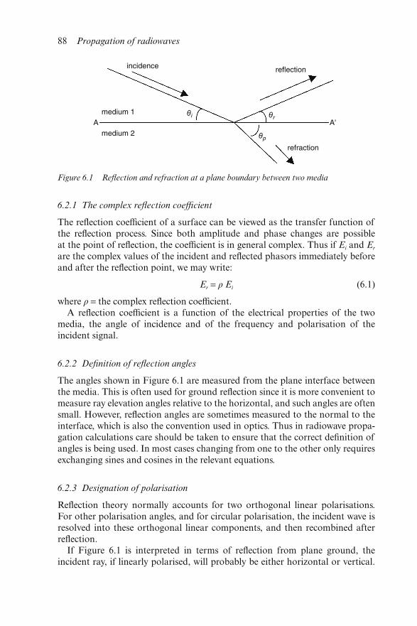
6.2.1 The complex reflection coefficient
The reflection coefficient of a surface can be viewed as the transfer function ofthe reflection process. Since both amplitude and phase changes are possibleat the point of reflection, the coefficient is in general complex. Thus if Ei and Er
are the complex values of the incident and reflected phasors immediately beforeand after the reflection point, we may write:
Er = ρ Ei (6.1)
where ρ = the complex reflection coefficient.A reflection coefficient is a function of the electrical properties of the two
media, the angle of incidence and of the frequency and polarisation of theincident signal.
6.2.2 Definition of reflection angles
The angles shown in Figure 6.1 are measured from the plane interface betweenthe media. This is often used for ground reflection since it is more convenient tomeasure ray elevation angles relative to the horizontal, and such angles are oftensmall. However, reflection angles are sometimes measured to the normal to theinterface, which is also the convention used in optics. Thus in radiowave propa-gation calculations care should be taken to ensure that the correct definition ofangles is being used. In most cases changing from one to the other only requiresexchanging sines and cosines in the relevant equations.
6.2.3 Designation of polarisation
Reflection theory normally accounts for two orthogonal linear polarisations.For other polarisation angles, and for circular polarisation, the incident wave isresolved into these orthogonal linear components, and then recombined afterreflection.
If Figure 6.1 is interpreted in terms of reflection from plane ground, theincident ray, if linearly polarised, will probably be either horizontal or vertical.
Figure 6.1 Reflection and refraction at a plane boundary between two media
88 Propagation of radiowaves
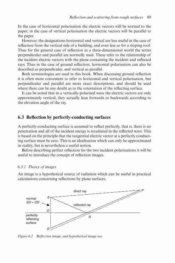
In the case of horizontal polarisation the electric vectors will be normal to thepaper; in the case of vertical polarisation the electric vectors will be parallel tothe paper.
However, the designations horizontal and vertical are less useful in the case ofreflection from the vertical side of a building, and even less so for a sloping roof.Thus for the general case of reflection in a three-dimensional world the termsperpendicular and parallel are normally used. These refer to the relationship ofthe incident electric vectors with the plane containing the incident and reflectedrays. Thus in the case of ground reflection, horizontal polarisation can also bedescribed as perpendicular, and vertical as parallel.
Both terminologies are used in this book. When discussing ground reflectionit is often more convenient to refer to horizontal and vertical polarisation, butperpendicular and parallel are more exact descriptions, and should be usedwhere there can be any doubt as to the orientation of the reflecting surface.
It can be noted that in a vertically-polarised wave the electric vectors are onlyapproximately vertical; they actually lean forwards or backwards according tothe elevation angle of the ray.
6.3 Reflection by perfectly-conducting surfaces
A perfectly-conducting surface is assumed to reflect perfectly, that is, there is nopenetration and all of the incident energy is reradiated in the reflected wave. Thisis based on the principle that the tangential electric vector at a perfectly conduct-ing surface must be zero. This is an idealisation which can only be approximatedin reality, but is nevertheless a useful notion.
Before describing perfect reflection for the two incident polarisations it will beuseful to introduce the concept of reflection images.
6.3.1 Theory of images
An image is a hypothetical source of radiation which can be useful in practicalcalculations concerning reflections by plane surfaces.
Figure 6.2 Reflection image, and hypothetical image ray
Reflection and scattering from rough surfaces 89
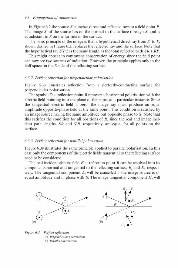
In Figure 6.2 the source S launches direct and reflected rays to a field point P.The image S′ of the source lies on the normal to the surface through S, and isequidistant to S on the far side of the surface.
The basic principle of the image is that a hypothetical direct ray from S′ to P,shown dashed in Figure 6.2, replaces the reflected ray and the surface. Note thatthe hypothetical ray S′P has the same length as the total reflected path SR + RP.
This might appear to contravene conservation of energy, since the field pointcan now see two sources of radiation. However, the principle applies only to thehalf space on the S side of the reflecting surface.
6.3.2 Perfect reflection for perpendicular polarisation
Figure 6.3a illustrates reflection from a perfectly-conducting surface forperpendicular polarisation.
The symbol ⊕ at reflection point R represents horizontal polarisation with theelectric field pointing into the plane of the paper at a particular instance. Sincethe tangential electric field is zero, the image ray must produce an equi-amplitude opposite-phase field at the same point. This condition is satisfied byan image source having the same amplitude but opposite phase to S. Note thatthis satisfies the condition for all positions of R, since the real and image inci-dent path lengths, SR and S′R, respectively, are equal for all points on thesurface.
6.3.3 Perfect reflection for parallel polarisation
Figure 6.3b illustrates the same principle applied to parallel polarisation. In thiscase only the components of the electric fields tangential to the reflecting surfaceneed to be considered.
The real incident electric field E at reflection point R can be resolved into itscomponents normal and tangential to the reflecting surface, En and Et, respect-ively. The tangential component Et will be cancelled if the image source is ofequal amplitude and in phase with S. The image tangential component E′t will
Figure 6.3 Perfect reflection(a) Perpendicular polarisation
(b) Parallel polarisation
90 Propagation of radiowaves
then be equal and opposite to Et, and again this will be true for any point on thesurface.
6.3.4 Discussion of perfect-reflection results
The above results suggest that for a perfect conductor the reflection coefficientwill be −1 + j.0 for perpendicular polarisation and 1 + j.0 for parallel polarisa-tion. In fact, as shown in the following section of this Chapter, for small inci-dence angles (relative to the surface) reflection coefficients tend in practice to beclose to −1 for both polarisations.
6.4 Reflection by finitely-conducting surfaces
The reflection coefficient at a general plane interface between two media can bederived from first principles as described below. Before doing so it will be con-venient to define the relevant electrical properties of media involved in thereflection.
6.4.1 Electrical properties relevant to reflection
The following electrical properties must be known for both media in order tocalculate the complex reflection coefficient at a plane boundary between them:
Permittivity:ε = ε0εr
where:
ε0 = permittivity of vacuum= 8.854.10−12 F m−1
εr = relative permittivity= 1.0 for vacuum (and to a good approximation for air)
Permeability:
μ = μ0μr
where:
μ0 = permeability of vacuum= 4 π.10−7 H m−1
μr = relative permeability= 1.0 for vacuum (and ≈ 1.0 for nonferromagnetics)
Two important characteristics of radiowaves are derived from these quantities:
wave impedance = √ (μ/ε)impedance of vacuum = √ (μ0/ε0) = 376.7 Ω
Reflection and scattering from rough surfaces 91
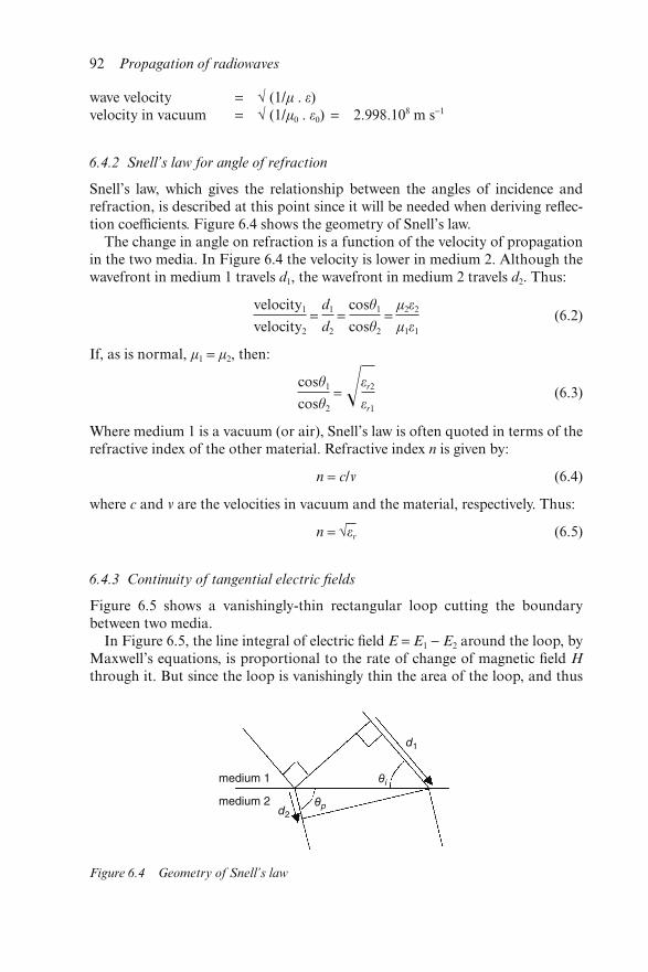
wave velocity = √ (1/μ . ε)velocity in vacuum = √ (1/μ0 . ε0) = 2.998.108 m s−1
6.4.2 Snell’s law for angle of refraction
Snell’s law, which gives the relationship between the angles of incidence andrefraction, is described at this point since it will be needed when deriving reflec-tion coefficients. Figure 6.4 shows the geometry of Snell’s law.
The change in angle on refraction is a function of the velocity of propagationin the two media. In Figure 6.4 the velocity is lower in medium 2. Although thewavefront in medium 1 travels d1, the wavefront in medium 2 travels d2. Thus:
velocity1
velocity2
= d1
d2
= cosθ1
cosθ2
= μ2ε2
μ1ε1
(6.2)
If, as is normal, μ1 = μ2, then:
cosθ1
cosθ2
= �εr2
εr1
(6.3)
Where medium 1 is a vacuum (or air), Snell’s law is often quoted in terms of therefractive index of the other material. Refractive index n is given by:
n = c/v (6.4)
where c and v are the velocities in vacuum and the material, respectively. Thus:
n = √εr (6.5)
6.4.3 Continuity of tangential electric fields
Figure 6.5 shows a vanishingly-thin rectangular loop cutting the boundarybetween two media.
In Figure 6.5, the line integral of electric field E = E1 − E2 around the loop, byMaxwell’s equations, is proportional to the rate of change of magnetic field Hthrough it. But since the loop is vanishingly thin the area of the loop, and thus
Figure 6.4 Geometry of Snell’s law
92 Propagation of radiowaves
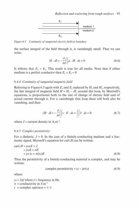
the surface integral of the field through it, is vanishingly small. Thus we canwrite:
E ⋅ dl = −δ
δt��μ ⋅ H ⋅ ds = 0 (6.6)
It follows that E1 = E2. This result is true for all media. Note that if eithermedium is a perfect conductor then E1 = E2 = 0.
6.4.4 Continuity of tangential magnetic field
Referring to Figure 6.5 again with E1 and E2 replaced by H1 and H2, respectively,the line integral of magnetic field H = H1 − H2 around this loop, by Maxwell’sequations, is proportional both to the rate of change of electric field and ofactual current through it. For a vanishingly thin loop these will both also bevanishing, and thus:
H ⋅ dl = −δ
δt�s
�ε ⋅ E ⋅ ds + �s
�J ⋅ ds = 0 (6.7)
where J = current density in A.m−2.
6.4.5 Complex permittivity
For a dieletric, J = 0. In the case of a finitely-conducting medium and a har-monic signal, Maxwell’s equation for curl.H can be written:
curl.H = jωεE + J= jωE + σE
= jω (ε + σ/jω)E (6.8)
Thus the permittivity of a finitely-conducting material is complex, and may bewritten:
complex permittivity = (ε − jσ/ω) (6.9)
where:
ω = 2πf where f = frequency in Hzσ = conductivity in S m−1
j = complex operator = √−1
Figure 6.5 Continuity of tangential electric field at boundary
Reflection and scattering from rough surfaces 93
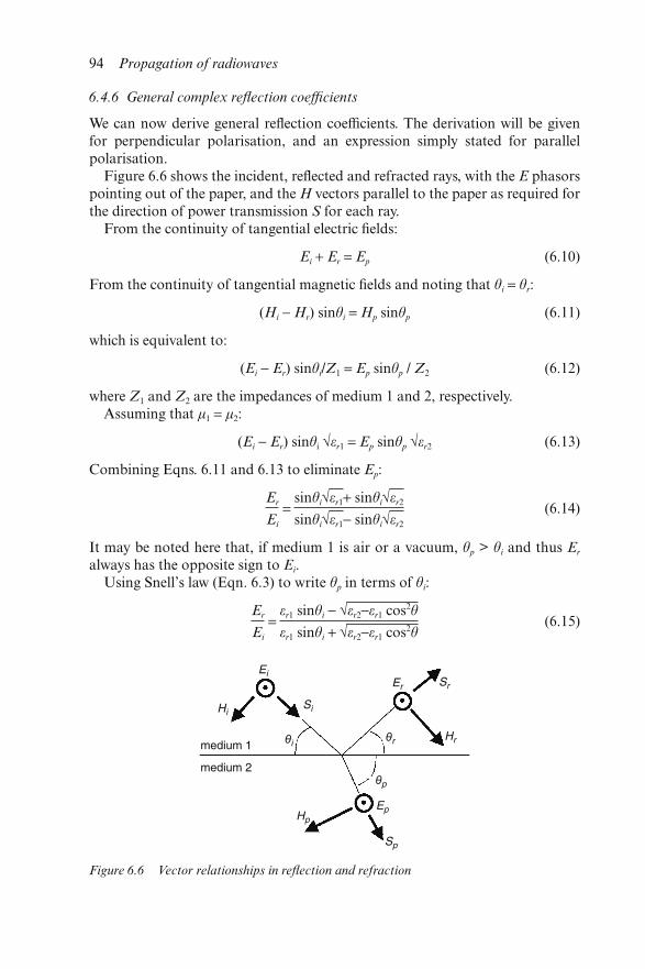
6.4.6 General complex reflection coefficients
We can now derive general reflection coefficients. The derivation will be givenfor perpendicular polarisation, and an expression simply stated for parallelpolarisation.
Figure 6.6 shows the incident, reflected and refracted rays, with the E phasorspointing out of the paper, and the H vectors parallel to the paper as required forthe direction of power transmission S for each ray.
From the continuity of tangential electric fields:
Ei + Er = Ep (6.10)
From the continuity of tangential magnetic fields and noting that θi = θr:
(Hi − Hr) sinθi = Hp sinθp (6.11)
which is equivalent to:
(Ei − Er) sinθi/Z1 = Ep sinθp / Z2 (6.12)
where Z1 and Z2 are the impedances of medium 1 and 2, respectively.Assuming that μ1 = μ2:
(Ei − Er) sinθi √εr1 = Ep sinθp √εr2 (6.13)
Combining Eqns. 6.11 and 6.13 to eliminate Ep:
Er
Ei
= sinθi√εr1+ sinθi√εr2
sinθi√εr1− sinθi√εr2
(6.14)
It may be noted here that, if medium 1 is air or a vacuum, θp > θi and thus Er
always has the opposite sign to Ei.Using Snell’s law (Eqn. 6.3) to write θp in terms of θi:
Er
Ei
= εr1 sinθi − √εr2−εr1 cos2θ
εr1 sinθi + √εr2−εr1 cos2θ(6.15)
Figure 6.6 Vector relationships in reflection and refraction
94 Propagation of radiowaves
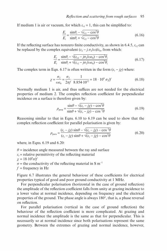
If medium 1 is air or vacuum, for which εr1 = 1, this can be simplified to:
Er
Ei
= sinθi − √εr2 − cos2θ
sinθi + √εr2 − cos2θ(6.16)
If the reflecting surface has nonzero finite conductivity, as shown in 6.4.5, εr2 canbe replaced by the complex equivalent (ε2 − j.σ2/ω)/ε0, from which:
Er
Ei
= sinθi − √(εr2 − jσ2/ωε0) − cos2θi
sinθi + √(εr2 − jσ2/ωε0) − cos2θi
(6.17)
The complex term in Eqn. 6.17 is often written in the form (εr − jχ) where:
χ = σ2
ωε0
= σ2
2πf ⋅
1
8.854⋅1012 = 18 ⋅ 109 σ2/f (6.18)
Normally medium 1 is air, and thus suffices are not needed for the electricalproperties of medium 2. The complex reflection coefficient for perpendicularincidence on a surface is therefore given by:
ρperp = sinθ − √(εr − jχ) − cos2θ
sinθ + √(εr − jχ) − cos 2θ(6.19)
Reasoning similar to that in Eqns. 6.10 to 6.19 can be used to show that thecomplex reflection coefficient for parallel polarisation is given by:
ρpara = (εr − jχ) sinθ − √(εr − jχ) − cos 2θ
(εr − jχ) sinθ + √(εr − jχ) − cos2θ(6.20)
where, in Eqns. 6.19 and 6.20:
θ = incidence angle measured between the ray and surfaceεr = relative permittivity of the reflecting materialχ = 18⋅109σ/fσ = the conductivity of the reflecting material in S m−1
f = frequency in Hz
Figure 6.7 illustrates the general behaviour of these coefficients for electricalproperties typical of good and poor ground conductivity at 1 MHz.
For perpendicular polarisation (horizontal in the case of ground reflection)the amplitude of the reflection coefficient falls from unity at grazing incidence toa lower value at normal incidence, depending on frequency and the electricalproperties of the ground. The phase angle is always 180°, that is, a phase reversalon reflection.
For parallel polarisation (vertical in the case of ground reflection) thebehaviour of the reflection coefficient is more complicated. At grazing andnormal incidence the amplitude is the same as that for perpendicular. This isnecessarily so at normal incidence since both polarisations represent the samegeometry. Between the extremes of grazing and normal incidence, however,
Reflection and scattering from rough surfaces 95
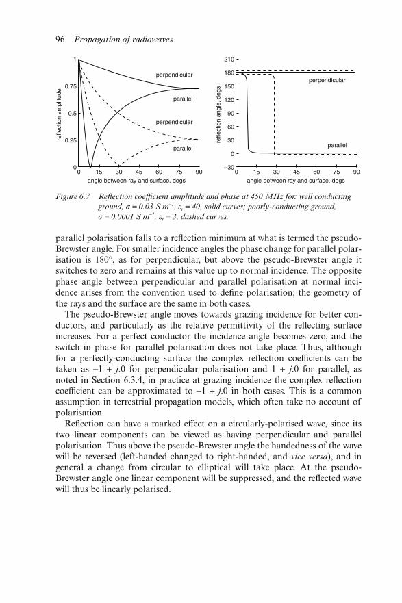
parallel polarisation falls to a reflection minimum at what is termed the pseudo-Brewster angle. For smaller incidence angles the phase change for parallel polar-isation is 180°, as for perpendicular, but above the pseudo-Brewster angle itswitches to zero and remains at this value up to normal incidence. The oppositephase angle between perpendicular and parallel polarisation at normal inci-dence arises from the convention used to define polarisation; the geometry ofthe rays and the surface are the same in both cases.
The pseudo-Brewster angle moves towards grazing incidence for better con-ductors, and particularly as the relative permittivity of the reflecting surfaceincreases. For a perfect conductor the incidence angle becomes zero, and theswitch in phase for parallel polarisation does not take place. Thus, althoughfor a perfectly-conducting surface the complex reflection coefficients can betaken as −1 + j.0 for perpendicular polarisation and 1 + j.0 for parallel, asnoted in Section 6.3.4, in practice at grazing incidence the complex reflectioncoefficient can be approximated to −1 + j.0 in both cases. This is a commonassumption in terrestrial propagation models, which often take no account ofpolarisation.
Reflection can have a marked effect on a circularly-polarised wave, since itstwo linear components can be viewed as having perpendicular and parallelpolarisation. Thus above the pseudo-Brewster angle the handedness of the wavewill be reversed (left-handed changed to right-handed, and vice versa), and ingeneral a change from circular to elliptical will take place. At the pseudo-Brewster angle one linear component will be suppressed, and the reflected wavewill thus be linearly polarised.
Figure 6.7 Reflection coefficient amplitude and phase at 450 MHz for: well conducting
ground, σ = 0.03 S m−1, εr = 40, solid curves; poorly-conducting ground,
σ = 0.0001 S m−1, εr = 3, dashed curves.
96 Propagation of radiowaves
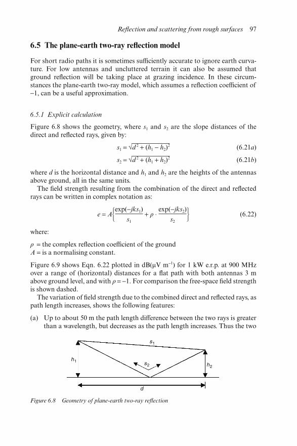
6.5 The plane-earth two-ray reflection model
For short radio paths it is sometimes sufficiently accurate to ignore earth curva-ture. For low antennas and uncluttered terrain it can also be assumed thatground reflection will be taking place at grazing incidence. In these circum-stances the plane-earth two-ray model, which assumes a reflection coefficient of−1, can be a useful approximation.
6.5.1 Explicit calculation
Figure 6.8 shows the geometry, where s1 and s2 are the slope distances of thedirect and reflected rays, given by:
s1 = √d 2 + (h1 − h2)2 (6.21a)
s2 = √d 2 + (h1 + h2)2 (6.21b)
where d is the horizontal distance and h1 and h2 are the heights of the antennasabove ground, all in the same units.
The field strength resulting from the combination of the direct and reflectedrays can be written in complex notation as:
e = A�exp(−jks1)
s1
+ ρ ⋅ exp(−jks2)
s2� (6.22)
where:
ρ = the complex reflection coefficient of the groundA = is a normalising constant.
Figure 6.9 shows Eqn. 6.22 plotted in dB(μV m−1) for 1 kW e.r.p. at 900 MHzover a range of (horizontal) distances for a flat path with both antennas 3 mabove ground level, and with ρ = −1. For comparison the free-space field strengthis shown dashed.
The variation of field strength due to the combined direct and reflected rays, aspath length increases, shows the following features:
(a) Up to about 50 m the path length difference between the two rays is greaterthan a wavelength, but decreases as the path length increases. Thus the two
Figure 6.8 Geometry of plane-earth two-ray reflection
Reflection and scattering from rough surfaces 97
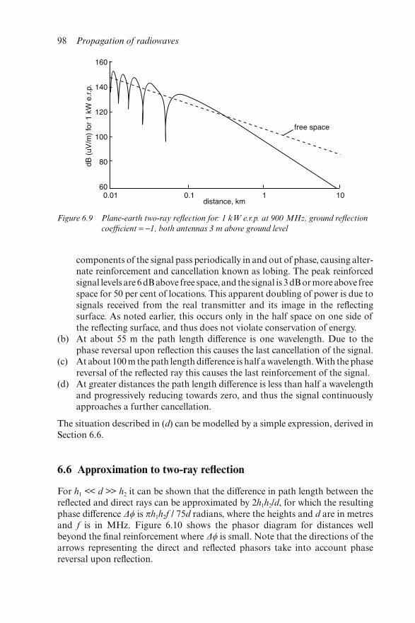
components of the signal pass periodically in and out of phase, causing alter-nate reinforcement and cancellation known as lobing. The peak reinforcedsignal levels are 6 dB above free space, and the signal is 3 dB or more above freespace for 50 per cent of locations. This apparent doubling of power is due tosignals received from the real transmitter and its image in the reflectingsurface. As noted earlier, this occurs only in the half space on one side ofthe reflecting surface, and thus does not violate conservation of energy.
(b) At about 55 m the path length difference is one wavelength. Due to thephase reversal upon reflection this causes the last cancellation of the signal.
(c) At about 100 m the path length difference is half a wavelength. With the phasereversal of the reflected ray this causes the last reinforcement of the signal.
(d) At greater distances the path length difference is less than half a wavelengthand progressively reducing towards zero, and thus the signal continuouslyapproaches a further cancellation.
The situation described in (d) can be modelled by a simple expression, derived inSection 6.6.
6.6 Approximation to two-ray reflection
For h1 << d >> h2 it can be shown that the difference in path length between thereflected and direct rays can be approximated by 2h1h2/d, for which the resultingphase difference Δ is πh1h2f / 75d radians, where the heights and d are in metresand f is in MHz. Figure 6.10 shows the phasor diagram for distances wellbeyond the final reinforcement where Δ is small. Note that the directions of thearrows representing the direct and reflected phasors take into account phasereversal upon reflection.
Figure 6.9 Plane-earth two-ray reflection for: 1 kW e.r.p. at 900 MHz, ground reflection
coefficient = −1, both antennas 3 m above ground level
98 Propagation of radiowaves
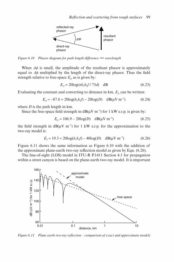
When Δ is small, the amplitude of the resultant phasor is approximatelyequal to Δ multiplied by the length of the direct-ray phasor. Thus the fieldstrength relative to free-space Efs as is given by:
Erf = 20log(πh1h2f / 75d) dB (6.23)
Evaluating the constant and converting to distance in km, Efs can be written:
Erf = −87.6 + 20log(h1h2f) − 20log(D) dB(μV m−1) (6.24)
where D is the path length in km.Since the free-space field strength in dB(μV m−1) for 1 kW e.r.p. is given by:
Efs = 106.9 − 20log(D) dB(μV m−1) (6.25)
the field strength in dB(μV m−1) for 1 kW e.r.p. for the approximation to thetwo-ray model is:
E2 = 19.3 + 20log(h1h2f) − 40log(D) dB(μV m−1) (6.26)
Figure 6.11 shows the same information as Figure 6.10 with the addition ofthe approximate plane-earth two-ray reflection model as given by Eqn. (6.26).
The line-of-sight (LOS) model in ITU-R P.1411 Section 4.1 for propagationwithin a street canyon is based on the plane-earth two-ray model. It is important
Figure 6.10 Phasor diagram for path length difference << wavelength
Figure 6.11 Plane earth two-ray reflection – comparison of exact and approximate models
Reflection and scattering from rough surfaces 99
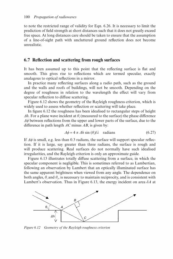
to note the restricted range of validity for Eqn. 6.26. It is necessary to limit theprediction of field strength at short distances such that it does not greatly exceedfree space. At long distances care should be taken to ensure that the assumptionof a line-of-sight path with uncluttered ground reflection does not becomeunrealistic.
6.7 Reflection and scattering from rough surfaces
It has been assumed up to this point that the reflecting surface is flat andsmooth. This gives rise to reflections which are termed specular, exactlyanalagous to optical reflections in a mirror.
In practice many reflecting surfaces along a radio path, such as the groundand the walls and roofs of buildings, will not be smooth. Depending on thedegree of roughness in relation to the wavelength the effect will vary fromspecular reflection to diffuse scattering.
Figure 6.12 shows the geometry of the Rayleigh roughness criterion, which iswidely used to assess whether reflection or scattering will take place.
In figure 6.12 the roughness has been idealised to rectangular steps of heightΔh. For a plane wave incident at θi (measured to the surface) the phase differenceΔ between reflections from the upper and lower parts of the surface, due to thedifference in path length AC minus AB, is given by:
Δ = 4 π Δh sin (θi)/λ radians (6.27)
If Δ is small, e.g. less than 0.3 radians, the surface will support specular reflec-tion. If it is large, say greater than three radians, the surface is rough andwill produce scattering. Real surfaces do not normally have such idealisedirregularities, and the Rayleigh criterion is only an approximate guide.
Figure 6.13 illustrates totally diffuse scattering from a surface, in which thespecular component is negligible. This is sometimes referred to as Lambertian,following an observation by Lambert that an optically illuminated surface hasthe same apparent brightness when viewed from any angle. The dependence onboth angles, θi and θs, is necessary to maintain reciprocity, and is consistent withLambert’s observation. Thus in Figure 6.13, the energy incident on area δA at
Figure 6.12 Geometry of the Rayleigh roughness criterion
100 Propagation of radiowaves
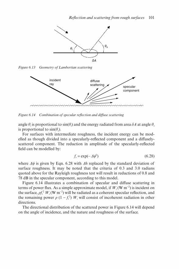
angle θi is proportional to sin(θi) and the energy radiated from area δA at angle θs
is proportional to sin(θs).For surfaces with intermediate roughness, the incident energy can be mod-
elled as though divided into a specularly-reflected component and a diffusely-scattered component. The reduction in amplitude of the specularly-reflectedfield can be modelled by:
fr = exp(−Δ2) (6.28)
where Δ is given by Eqn. 6.28 with Δh replaced by the standard deviation ofsurface roughness. It may be noted that the criteria of 0.3 and 3.0 radiansquoted above for the Rayleigh roughness test will result in reductions of 0.8 and78 dB in the specular component, according to this model.
Figure 6.14 illustrates a combination of specular and diffuse scattering interms of power flux. As a simple approximate model, if Wi (W m−2) is incident onthe surface, ρfr
2 Wi (W m−2) will be radiated as a coherent specular reflection, andthe remaining power ρ (1 − fr
2) Wi will consist of incoherent radiation in otherdirections.
The directional distribution of the scattered power in Figure 6.14 will dependon the angle of incidence, and the nature and roughness of the surface.
Figure 6.13 Geometry of Lambertian scattering
Figure 6.14 Combination of specular reflection and diffuse scattering
Reflection and scattering from rough surfaces 101

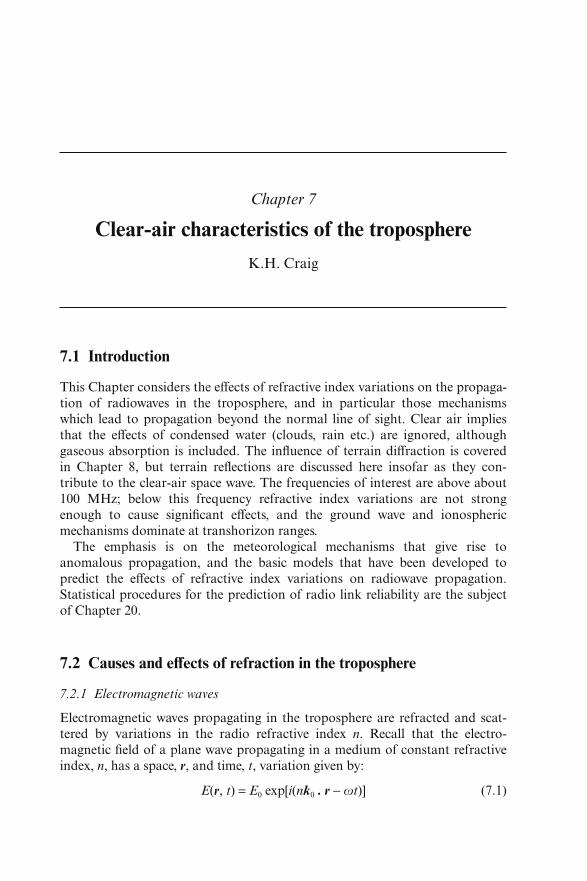
Chapter 7
Clear-air characteristics of the troposphere
K.H. Craig
7.1 Introduction
This Chapter considers the effects of refractive index variations on the propaga-tion of radiowaves in the troposphere, and in particular those mechanismswhich lead to propagation beyond the normal line of sight. Clear air impliesthat the effects of condensed water (clouds, rain etc.) are ignored, althoughgaseous absorption is included. The influence of terrain diffraction is coveredin Chapter 8, but terrain reflections are discussed here insofar as they con-tribute to the clear-air space wave. The frequencies of interest are above about100 MHz; below this frequency refractive index variations are not strongenough to cause significant effects, and the ground wave and ionosphericmechanisms dominate at transhorizon ranges.
The emphasis is on the meteorological mechanisms that give rise toanomalous propagation, and the basic models that have been developed topredict the effects of refractive index variations on radiowave propagation.Statistical procedures for the prediction of radio link reliability are the subjectof Chapter 20.
7.2 Causes and effects of refraction in the troposphere
7.2.1 Electromagnetic waves
Electromagnetic waves propagating in the troposphere are refracted and scat-tered by variations in the radio refractive index n. Recall that the electro-magnetic field of a plane wave propagating in a medium of constant refractiveindex, n, has a space, r, and time, t, variation given by:
E(r, t) = E0 exp[i(nk0 . r − ωt)] (7.1)
where ω = 2π × frequency and k0 is a vector normal to the wavefront with amagnitude equal to the free space wavenumber (= 2π/wavelength).
In the troposphere, the refractive index is not constant. At microwave fre-quencies, however, it varies slowly on the scale of a wavelength. In this case it isstill possible to write:
E(r,t) ≈ E0 exp[i(n(r)k0 . r − ωt)] (7.2)
although the magnitude of E(r,t) will in general vary with position. The valueand variations of n(r) are fundamental to understanding the way in which elec-tromagnetic waves propagate through the troposphere. For example, Snell’s lawof refraction and the Fresnel coefficients for reflection and transmission at aninterface follow from Eqn. 7.2 by applying appropriate boundary conditionsacross a boundary separating media of different refractive indices. In thisChapter we are principally interested in refractive effects. We first consider thedetermination of n in the troposphere.
7.2.2 Radio refractive index
The radio refractive index of the troposphere is due to the molecular constitu-ents of the air, principally nitrogen, oxygen, carbon dioxide and water vapour.The value of n deviates from unity because of the polarisability of these mol-ecules due to the incident electromagnetic field, and quantum mechanicalmolecular resonances. The latter effect is limited to narrow frequency bands (forexample, around 22 GHz and 60 GHz). We first discuss the former effect whichis independent of frequency at the frequencies of interest (up to millimetrewaves).
The deviation of n from unity is very small in absolute terms, a typical valuebeing 1.0003 at the earth’s surface. Because of the closeness of n to unity, it isusual to work with the refractivity, N, defined by:
N = (n − 1) × 106 (7.3)
N is dimensionless, but for convenience is measured in N units. N depends on thepressure P (mbar), the absolute temperature T (K) and the partial pressure ofwater vapour e (mbar):
N = 77.6 P
T + 3.73 × 10⁵
e
T 2(7.4)
This is derived from the Debye formula [1] for the polarisability of polar (i.e.with a strong permanent electric dipole moment) and nonpolar molecules. Thefirst (dry) term is due principally to the nonpolar nitrogen and oxygen mol-ecules, and the second (wet) term is from the polar water vapour molecules. Theconstants are empirically determined, based on experimental measurements [2].An excellent discussion of Eqn. 7.4 is given in Reference [3].
The variation of P, T and e can be considered at various scales:
104 Propagation of radiowaves
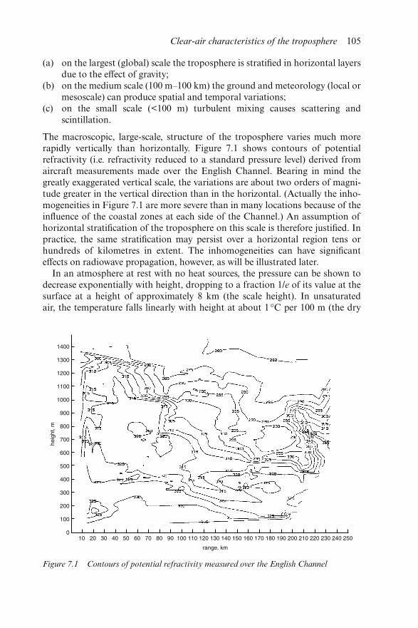
(a) on the largest (global) scale the troposphere is stratified in horizontal layersdue to the effect of gravity;
(b) on the medium scale (100 m–100 km) the ground and meteorology (local ormesoscale) can produce spatial and temporal variations;
(c) on the small scale (<100 m) turbulent mixing causes scattering andscintillation.
The macroscopic, large-scale, structure of the troposphere varies much morerapidly vertically than horizontally. Figure 7.1 shows contours of potentialrefractivity (i.e. refractivity reduced to a standard pressure level) derived fromaircraft measurements made over the English Channel. Bearing in mind thegreatly exaggerated vertical scale, the variations are about two orders of magni-tude greater in the vertical direction than in the horizontal. (Actually the inho-mogeneities in Figure 7.1 are more severe than in many locations because of theinfluence of the coastal zones at each side of the Channel.) An assumption ofhorizontal stratification of the troposphere on this scale is therefore justified. Inpractice, the same stratification may persist over a horizontal region tens orhundreds of kilometres in extent. The inhomogeneities can have significanteffects on radiowave propagation, however, as will be illustrated later.
In an atmosphere at rest with no heat sources, the pressure can be shown todecrease exponentially with height, dropping to a fraction 1/e of its value at thesurface at a height of approximately 8 km (the scale height). In unsaturatedair, the temperature falls linearly with height at about 1 °C per 100 m (the dry
Figure 7.1 Contours of potential refractivity measured over the English Channel
Clear-air characteristics of the troposphere 105
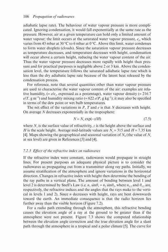
adiabatic lapse rate). The behaviour of water vapour pressure is more compli-cated. Ignoring condensation, it would fall exponentially at the same rate as thepressure. However, air at a given temperature can hold only a limited amount ofwater vapour; the limit occurs at the saturated water vapour pressure, es, whichvaries from 43 mbar at 30 °C to 6 mbar at 0 °C. Above this limit, water condensesto form water droplets (clouds). Since the saturation vapour pressure decreasesas temperature decreases, and temperature decreases with height, condensationwill occur above a certain height, reducing the water vapour content of the air.Thus the water vapour pressure decreases more rapidly with height than pres-sure and for practical purposes is negligible above 2 or 3 km. Above the conden-sation level, the temperature follows the saturated adiabatic lapse rate which isless than the dry adiabatic lapse rate because of the latent heat released by thecondensation process.
For reference, note that several quantities other than water vapour pressureare used to characterise the water vapour content of the air: examples are rela-tive humidity, (= e/es, expressed as a percentage), water vapour density (= 216.7e/T, g m−3) and humidity mixing ratio (= 622 e/P, g kg−1); it may also be specifiedin terms of the dew point or wet bulb temperatures.
The net effect of the variations in P, T and e is that N decreases with height.On average N decreases exponentially in the troposphere:
N = Ns exp(−z/H) (7.5)
where Ns is the surface value of refractivity, z is the height above the surface andH is the scale height. Average mid-latitude values are Ns = 315 and H = 7.35 km[4]. Maps showing the geographical and seasonal variation of N0 (the value of Ns
at sea level) are given in References [3] and [4].
7.2.3 Effect of the refractive index on radiowaves
If the refractive index were constant, radiowaves would propagate in straightlines. For present purposes an adequate physical picture is to consider theradiowaves as propagating out from a transmitter along ray paths. Initially, weassume stratification of the atmosphere and ignore variations in the horizontaldirection. Changes in refractive index with height then determine the bending ofthe ray paths in a vertical plane. The amount of bending between level 1 andlevel 2 is determined by Snell’s Law (i.e. n1 sinθ1 = n2 sinθ2, where n1,2 and θ1,2 are,respectively, the refractive indices and the angles that the rays make to the verti-cal in levels 1 and 2). Since n decreases with height, rays are bent downwardstoward the earth. An immediate consequence is that the radio horizon liesfurther away than the visible horizon (Figure 7.2).
For a radio path extending through the atmosphere, this refractive bendingcauses the elevation angle of a ray at the ground to be greater than if theatmosphere were not present. Figure 7.3 shows the computed relationshipbetween the elevation angle correction and the true elevation angle for a slantpath through the atmosphere in a tropical and a polar climate [5]. The curve for
106 Propagation of radiowaves
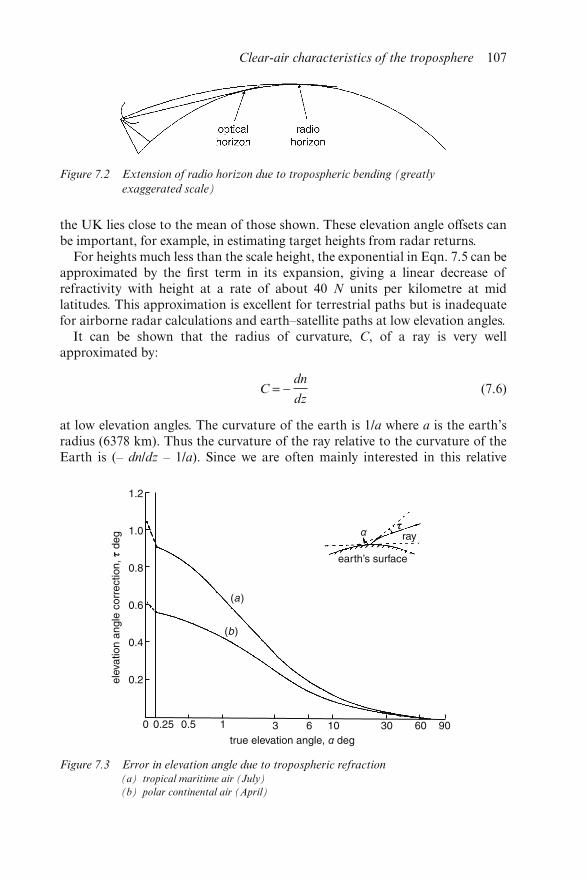
the UK lies close to the mean of those shown. These elevation angle offsets canbe important, for example, in estimating target heights from radar returns.
For heights much less than the scale height, the exponential in Eqn. 7.5 can beapproximated by the first term in its expansion, giving a linear decrease ofrefractivity with height at a rate of about 40 N units per kilometre at midlatitudes. This approximation is excellent for terrestrial paths but is inadequatefor airborne radar calculations and earth–satellite paths at low elevation angles.
It can be shown that the radius of curvature, C, of a ray is very wellapproximated by:
C = − dn
dz(7.6)
at low elevation angles. The curvature of the earth is 1/a where a is the earth’sradius (6378 km). Thus the curvature of the ray relative to the curvature of theEarth is (– dn/dz – 1/a). Since we are often mainly interested in this relative
Figure 7.2 Extension of radio horizon due to tropospheric bending (greatly
exaggerated scale)
Figure 7.3 Error in elevation angle due to tropospheric refraction(a) tropical maritime air (July)
(b) polar continental air (April)
Clear-air characteristics of the troposphere 107
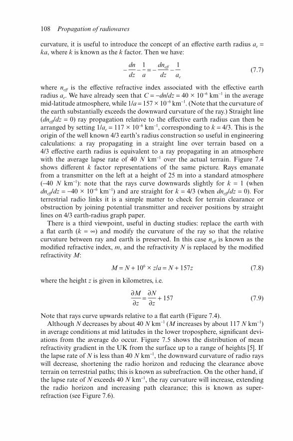
curvature, it is useful to introduce the concept of an effective earth radius ae =ka, where k is known as the k factor. Then we have:
−dn
dz−
1
a= −
dneff
dz−
1
ae
(7.7)
where neff is the effective refractive index associated with the effective earthradius ae. We have already seen that C = −dn/dz = 40 × 10−6 km−1 in the averagemid-latitude atmosphere, while 1/a = 157 × 10−6 km−1. (Note that the curvature ofthe earth substantially exceeds the downward curvature of the ray.) Straight line(dneff/dz = 0) ray propagation relative to the effective earth radius can then bearranged by setting 1/ae = 117 × 10−6 km−1, corresponding to k = 4/3. This is theorigin of the well known 4/3 earth’s radius construction so useful in engineeringcalculations: a ray propagating in a straight line over terrain based on a4/3 effective earth radius is equivalent to a ray propagating in an atmospherewith the average lapse rate of 40 N km−1 over the actual terrain. Figure 7.4shows different k factor representations of the same picture. Rays emanatefrom a transmitter on the left at a height of 25 m into a standard atmosphere(−40 N km−1): note that the rays curve downwards slightly for k = 1 (whendneff/dz = −40 × 10−6 km−1) and are straight for k = 4/3 (when dneff/dz = 0). Forterrestrial radio links it is a simple matter to check for terrain clearance orobstruction by joining potential transmitter and receiver positions by straightlines on 4/3 earth-radius graph paper.
There is a third viewpoint, useful in ducting studies: replace the earth witha flat earth (k = ∞) and modify the curvature of the ray so that the relativecurvature between ray and earth is preserved. In this case neff is known as themodified refractive index, m, and the refractivity N is replaced by the modifiedrefractivity M:
M = N + 106 × z/a = N + 157z (7.8)
where the height z is given in kilometres, i.e.
∂M
∂z =
∂N
∂z + 157 (7.9)
Note that rays curve upwards relative to a flat earth (Figure 7.4).Although N decreases by about 40 N km−1 (M increases by about 117 N km−1)
in average conditions at mid latitudes in the lower troposphere, significant devi-ations from the average do occur. Figure 7.5 shows the distribution of meanrefractivity gradient in the UK from the surface up to a range of heights [5]. Ifthe lapse rate of N is less than 40 N km−1, the downward curvature of radio rayswill decrease, shortening the radio horizon and reducing the clearance aboveterrain on terrestrial paths; this is known as subrefraction. On the other hand, ifthe lapse rate of N exceeds 40 N km−1, the ray curvature will increase, extendingthe radio horizon and increasing path clearance; this is known as super-refraction (see Figure 7.6).
108 Propagation of radiowaves
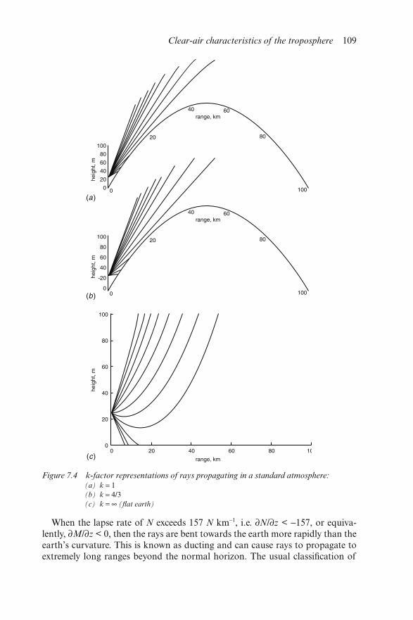
When the lapse rate of N exceeds 157 N km−1, i.e. ∂N/∂z < −157, or equiva-lently, ∂M/∂z < 0, then the rays are bent towards the earth more rapidly than theearth’s curvature. This is known as ducting and can cause rays to propagate toextremely long ranges beyond the normal horizon. The usual classification of
Figure 7.4 k-factor representations of rays propagating in a standard atmosphere:(a) k = 1(b) k = 4/3(c) k = ∞ (flat earth)
Clear-air characteristics of the troposphere 109
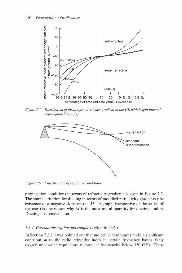
propagation conditions in terms of refractivity gradients is given in Figure 7.7.The simple criterion for ducting in terms of modified refractivity gradients (theexistence of a negative slope on the M − z graph, irrespective of the scales ofthe axes) is one reason why M is the most useful quantity for ducting studies.Ducting is discussed later.
7.2.4 Gaseous absorption and complex refractive index
In Section 7.2.2 it was pointed out that molecular resonances make a significantcontribution to the radio refractive index in certain frequency bands. Onlyoxygen and water vapour are relevant at frequencies below 350 GHz. These
Figure 7.5 Distribution of mean refractive index gradient in the UK with height interval
above ground level [5]
Figure 7.6 Classification of refractive conditions
110 Propagation of radiowaves
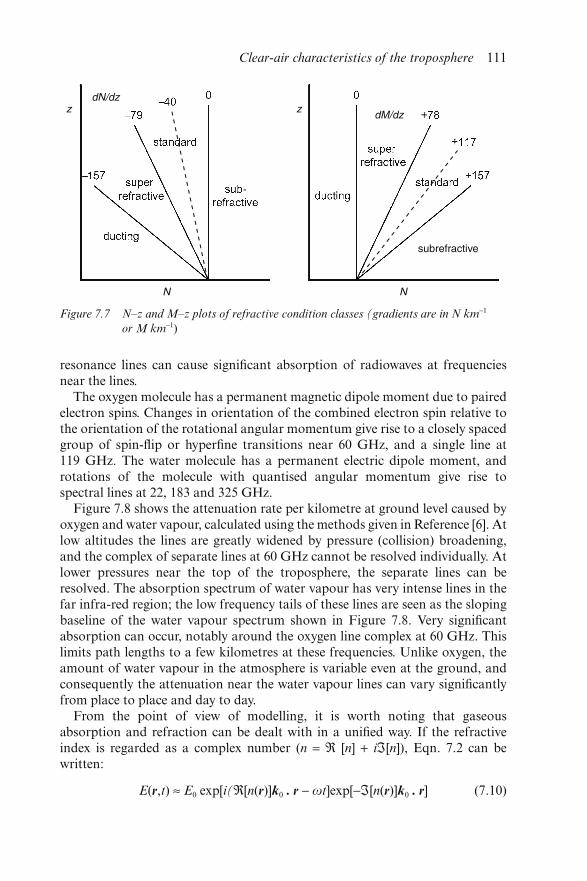
resonance lines can cause significant absorption of radiowaves at frequenciesnear the lines.
The oxygen molecule has a permanent magnetic dipole moment due to pairedelectron spins. Changes in orientation of the combined electron spin relative tothe orientation of the rotational angular momentum give rise to a closely spacedgroup of spin-flip or hyperfine transitions near 60 GHz, and a single line at119 GHz. The water molecule has a permanent electric dipole moment, androtations of the molecule with quantised angular momentum give rise tospectral lines at 22, 183 and 325 GHz.
Figure 7.8 shows the attenuation rate per kilometre at ground level caused byoxygen and water vapour, calculated using the methods given in Reference [6]. Atlow altitudes the lines are greatly widened by pressure (collision) broadening,and the complex of separate lines at 60 GHz cannot be resolved individually. Atlower pressures near the top of the troposphere, the separate lines can beresolved. The absorption spectrum of water vapour has very intense lines in thefar infra-red region; the low frequency tails of these lines are seen as the slopingbaseline of the water vapour spectrum shown in Figure 7.8. Very significantabsorption can occur, notably around the oxygen line complex at 60 GHz. Thislimits path lengths to a few kilometres at these frequencies. Unlike oxygen, theamount of water vapour in the atmosphere is variable even at the ground, andconsequently the attenuation near the water vapour lines can vary significantlyfrom place to place and day to day.
From the point of view of modelling, it is worth noting that gaseousabsorption and refraction can be dealt with in a unified way. If the refractiveindex is regarded as a complex number (n = ℜ [n] + iℑ[n]), Eqn. 7.2 can bewritten:
E(r,t) ≈ E0 exp[i(ℜ[n(r)]k0 . r − ωt]exp[−ℑ[n(r)]k0 . r] (7.10)
Figure 7.7 N–z and M–z plots of refractive condition classes (gradients are in N km−1
or M km−1)
Clear-air characteristics of the troposphere 111
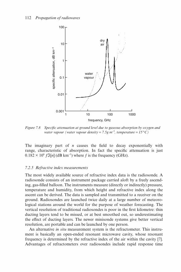
The imaginary part of n causes the field to decay exponentially withrange, characteristic of absorption. In fact the specific attenuation is just0.182 × 106 ƒℑ[n] (dB km−1) where ƒ is the frequency (GHz).
7.2.5 Refractive index measurements
The most widely available source of refractive index data is the radiosonde. Aradiosonde consists of an instrument package carried aloft by a freely ascend-ing, gas-filled balloon. The instruments measure (directly or indirectly) pressure,temperature and humidity, from which height and refractive index along theascent can be derived. The data is sampled and transmitted to a receiver on theground. Radiosondes are launched twice daily at a large number of meteoro-logical stations around the world for the purpose of weather forecasting. Thevertical resolution of traditional radiosondes is poor in the first kilometre: thinducting layers tend to be missed, or at best smoothed out, so underestimatingthe effect of ducting layers. The newer minisonde systems give better verticalresolution, are portable and can be launched by one person.
An alternative in situ measurement system is the refractometer. This instru-ment is basically an open-ended resonant microwave cavity, whose resonantfrequency is determined by the refractive index of the air within the cavity [7].Advantages of refractometers over radiosondes include rapid response time
Figure 7.8 Specific attenuation at ground level due to gaseous absorption by oxygen and
water vapour (water vapour density = 7.5g m−3, temperature = 15 °C)
112 Propagation of radiowaves
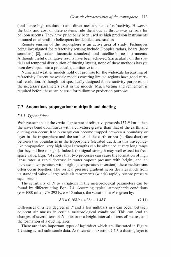
(and hence high resolution) and direct measurement of refractivity. However,the bulk and cost of these systems rule them out as throw-away sensors forballoon ascents. They have principally been used as high precision instrumentsmounted on aircraft or helicopters for detailed case studies.
Remote sensing of the troposphere is an active area of study. Techniquesbeing investigated for refractivity sensing include Doppler radars, lidars (lasersounders) [8], sodars (acoustic sounders) and satellite-borne instruments.Although useful qualitative results have been achieved (particularly on the spa-tial and temporal distribution of ducting layers), none of these methods has yetbeen developed into a practical, quantitative tool.
Numerical weather models hold out promise for the widescale forecasting ofrefractivity. Recent mesoscale models covering limited regions have good verti-cal resolution. Although not specifically designed for refractivity purposes, allthe necessary parameters exist in the models. Much testing and refinement isrequired before these can be used for radiowave prediction purposes.
7.3 Anomalous propagation: multipath and ducting
7.3.1 Types of duct
We have seen that if the vertical lapse rate of refractivity exceeds 157 N km−1, thenthe waves bend downwards with a curvature greater than that of the earth, andducting can occur. Radio energy can become trapped between a boundary orlayer in the troposphere and the surface of the earth or sea (surface duct) orbetween two boundaries in the troposphere (elevated duct). In this waveguide-like propagation, very high signal strengths can be obtained at very long range(far beyond line of sight). Indeed, the signal strength may well exceed its free-space value. Eqn. 7.4 shows that two processes can cause the formation of highlapse rates: a rapid decrease in water vapour pressure with height, and anincrease in temperature with height (a temperature inversion); these mechanismsoften occur together. The vertical pressure gradient never deviates much fromits standard value – large scale air movements (winds) rapidly restore pressureequilibrium.
The sensitivity of N to variations in the meteorological parameters can befound by differentiating Eqn. 7.4. Assuming typical atmospheric conditions(P = 1000 mbar, T = 293 K, e = 15 mbar), the variation in N is given by:
δN = 0.26δP + 4.3δe − 1.4δT (7.11)
Differences of a few degrees in T and a few millibars in e can occur betweenadjacent air masses in certain meteorological conditions. This can lead tochanges of several tens of N units over a height interval of tens of metres, andthe formation of a ducting layer.
There are three important types of layer/duct which are illustrated in Figure7.9 using actual radiosonde data. As discussed in Section 7.2.3, a ducting layer is
Clear-air characteristics of the troposphere 113
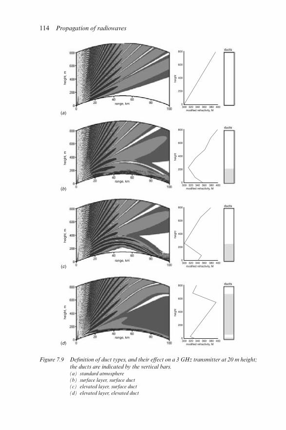
Figure 7.9 Definition of duct types, and their effect on a 3 GHz transmitter at 20 m height;
the ducts are indicated by the vertical bars.(a) standard atmosphere
(b) surface layer, surface duct
(c) elevated layer, surface duct
(d) elevated layer, elevated duct
114 Propagation of radiowaves
immediately identifiable by a negative slope in the modified refractivity–heightcurve; the duct (marked by a vertical bar in Figure 7.9) extends from the top ofthe ducting layer down to the ground (in the case of a surface duct) or down tothe height at which the modified refractivity returns to the same value as at thetop of the layer (in the case of an elevated duct).
Figure 7.9a shows the standard atmosphere for reference. Figure 7.9b shows asurface duct caused by a surface layer. Figures 7.9c and d show elevated layers:Figure 7.9c forms a surface duct, while Figure 7.9d forms an elevated duct. Itshould be borne in mind that the refractivity profiles can be complicated andmultiple layers do occur (such as the low surface duct in Figure 7.9d accompany-ing the elevated duct); nevertheless the concept of surface and elevated ducts isuseful. In northern Europe, surface ducts occur for about 5 per cent, and ele-vated ducts for 5–10 per cent, of the time, averaged over the year. The percentageof the time that a radio link is affected by ducting will in general be less thanthese figures, because of the importance of the path geometry relative to theducting layers.
The contour plots show the effect of the associated layers on a 3 GHz trans-mitter located on the left at a height of 20 m over the sea; the contours are givenin terms of path loss. The common feature in all the plots is the lobing caused byinterference between energy arriving at a point via the direct and groundreflected paths. The term multipath is often used to describe the situation whereradiowaves propagate from transmitter to receiver by more than one path,especially on a line-of-sight link. The secondary paths may occur by groundreflection (as here) or by refraction. The distinction between ducting and multi-path caused by interference between two or more refractive paths through theatmosphere is more a descriptive convenience than a fundamental difference inmechanism. At longer (transhorizon) ranges, the number of multiple pathsbecomes very large, and it is more appropriate to use models based on ductingtheory. The effects of multipath on terrestrial line-of-sight paths are discussed inChapter 20.
The distance to the normal radio horizon, d (km), is given in terms of thetransmitter height, h (m) by:
d = 4.12 √h (7.12)
Both types of surface duct are seen to propagate energy well beyond the normalradio horizon (at 18.4 km range for a 20 m high transmitter). However, notethe skip zone that occurs in the elevated layer, surface duct example.
A ducting layer will only trap radiowaves if certain geometrical constraintsapply. In particular, the angle of incidence of electromagnetic energy at the layermust be very small. A simple rule of thumb, derived from the total-internal-reflection condition of geometrical optics, is that the maximum angle of inci-dence θmax (degrees) is related to the change in refractivity ΔN (N units) acrossthe layer by:
θmax = 0.081√|ΔN| (7.13)
Clear-air characteristics of the troposphere 115
As ΔN rarely exceeds 50 N units, θmax will be limited to 0.5–1°. Simplegeometrical considerations show that even energy launched horizontally willintercept an elevated layer at a nonzero angle due to the earth’s curvature. Itfollows that ducting layers higher than about 1 km will not significantly affectterrestrial radio links. For example, although the elevated duct of Figure 7.9d
distorts the interference lobes significantly, it is not strong enough to trap theenergy completely.
The dependence of ducted field strength on frequency and path geometry iscomplicated. At long ranges from the transmitter, a simple single mode propaga-tion model of a surface duct (see Section 7.4.3) predicts that the field strengthshould decrease exponentially with distance (i.e. linear in decibels) because ofmode attenuation. This is indeed reflected in the ITU-R prediction method forthe prediction of interference levels caused by ducting and layer reflection (seeChapter 20, Figure 20.17, where γd represents the specific attenuation of theduct). However, the attenuation rate should theoretically become smaller athigher frequencies for a uniform duct; this is opposite to what is observed (seeSection 20.9.5.2), indicating that horizontal inhomogeneities and small scalescatter begin to be important at microwave frequencies. The strongest couplingof energy into or out of a duct occurs when the transmitter or receiver itselflies within the duct: the ITU-R prediction method incorporates an antennaheight-dependent factor to account for coupling into coastal advection ducts.
If the change in refractivity between two air masses is very abrupt, it is moreappropriate to consider the radiowaves to be reflected by the layer, rather thanrefracted by it. A layer of thickness t can be considered to be a discontinuity if:
t < 14 λ/θ (7.14)
where λ is the wavelength (in the same units as t) and θ is the angle of incidence(degrees). In this case the strength of the field reflected and transmitted by thelayer can be calculated by means of Fresnel’s formulae for reflection and trans-mission coefficients. From Eqn. 7.14 the distinction between refraction andreflection is frequency dependent, and is really a choice in the way the mechan-ism is modelled, rather than a difference in the mechanism itself. The layerreflection model is most useful at lower (VHF) frequencies, while refraction/ducting is a better model at UHF and above.
The meteorological mechanisms causing duct formation are now discussed.More details can be found in References [3] and [9].
7.3.2 Evaporation
A shallow surface-based duct, the evaporation duct, exists for most of the timeover the sea (and other large bodies of water), caused by the very rapid decreaseof water vapour pressure with height in the lowest few metres above the seasurface. The mean duct thickness varies with geographical location, rangingfrom 5–6 m in the North Sea through 13–14 m in the Mediterranean to over20 m in the Gulf area. The evaporation duct is the dominant propagation
116 Propagation of radiowaves
mechanism for ship-based radar and communication systems. It can also havean important modifying effect at coastal sites in the presence of other surfaceducts, such as the advection duct described below.
Because of its influence on naval sensor performance, much effort has goneinto understanding the evaporation duct. There are well established boundarylayer models [10–13] based on the similarity theory of turbulence; these enablethe evaporation duct height to be estimated from a bulk measurement of seatemperature, and the air temperature, water vapour pressure and wind velocity afew metres above the surface. In open ocean conditions where the sea tempera-ture and meteorology vary relatively slowly with range, the evaporation duct canextend for hundreds of kilometres with almost constant duct height. In coastalregions, and in enclosed areas such as the Gulf area, significant variations induct height can occur.
Figure 7.10 shows the effect of a 15 m evaporation duct on the coverage of aradar at a height of 25 m above the sea at 3 GHz (S band) and 18 GHz (Kuband). The contours here are given in terms of propagation factor (field strengthrelative to free space); this is a better quantity than path loss for comparingsystems operating at different frequencies. Note that the effects are stronger atthe higher frequency, and that the interference lobes are trapped in the duct eventhough the antenna lies above the duct.
7.3.3 Nocturnal radiation
Radiative heat loss from the ground during clear, still nights produces a tempera-ture inversion. This can result in the formation of a duct over inland or coastalregions, depending on the humidity profile. If there is sufficient water vapourpresent, condensation can occur, forming a radiative fog; the temperature inver-sion will cause an increase in water vapour pressure with height, leading tosubrefraction. On the other hand, if the air is dry, the temperature inversioncauses super refraction and ducting. In dry, hot climates (such as North Africaor the Middle East), radiation inversions cause severe problems to broadcastservices [14].
The inversion layer weakens after sunrise, and is finally destroyed by solarheating. Hence periods of anomalous propagation associated with nocturnalradiation ducting are fairly short (one or two hours). In northern Europe thistype of ducting tends to be localised, since it depends on the nature of theground cover and of local topographical features. It is therefore less likely thanother forms of ducting to cause interference over long distances. However, it cancause a severe multipath problem for low lying terrestrial links, particularlywhen the ducting layers are in the process of forming and breaking up.
7.3.4 Subsidence inversion
Elevated ducts can be formed by large scale atmospheric subsidence occurringduring anticyclonic conditions. Large cooler air masses associated with high
Clear-air characteristics of the troposphere 117
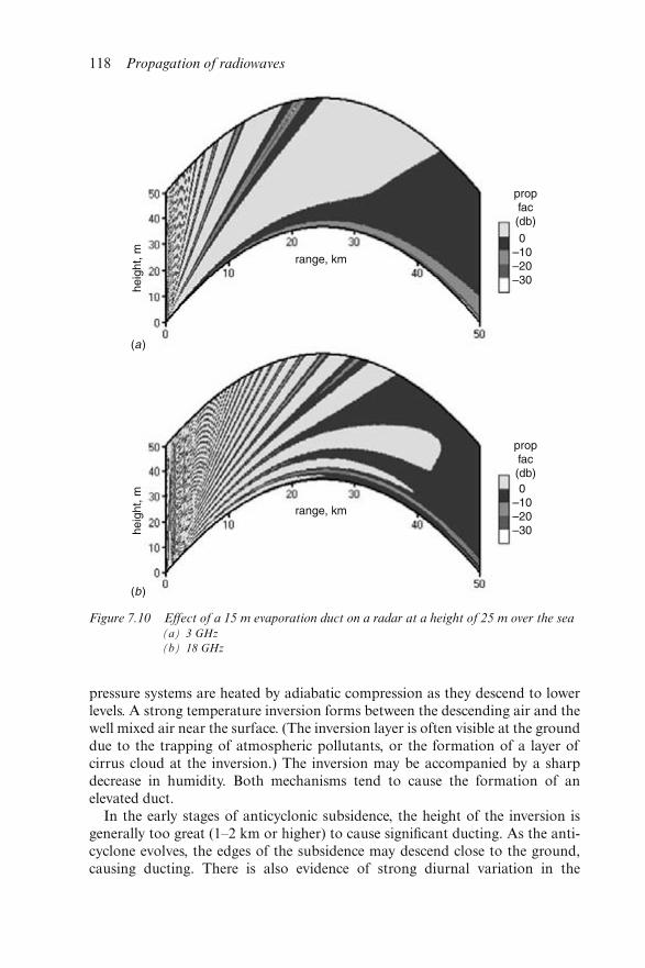
pressure systems are heated by adiabatic compression as they descend to lowerlevels. A strong temperature inversion forms between the descending air and thewell mixed air near the surface. (The inversion layer is often visible at the grounddue to the trapping of atmospheric pollutants, or the formation of a layer ofcirrus cloud at the inversion.) The inversion may be accompanied by a sharpdecrease in humidity. Both mechanisms tend to cause the formation of anelevated duct.
In the early stages of anticyclonic subsidence, the height of the inversion isgenerally too great (1–2 km or higher) to cause significant ducting. As the anti-cyclone evolves, the edges of the subsidence may descend close to the ground,causing ducting. There is also evidence of strong diurnal variation in the
Figure 7.10 Effect of a 15 m evaporation duct on a radar at a height of 25 m over the sea(a) 3 GHz
(b) 18 GHz
118 Propagation of radiowaves
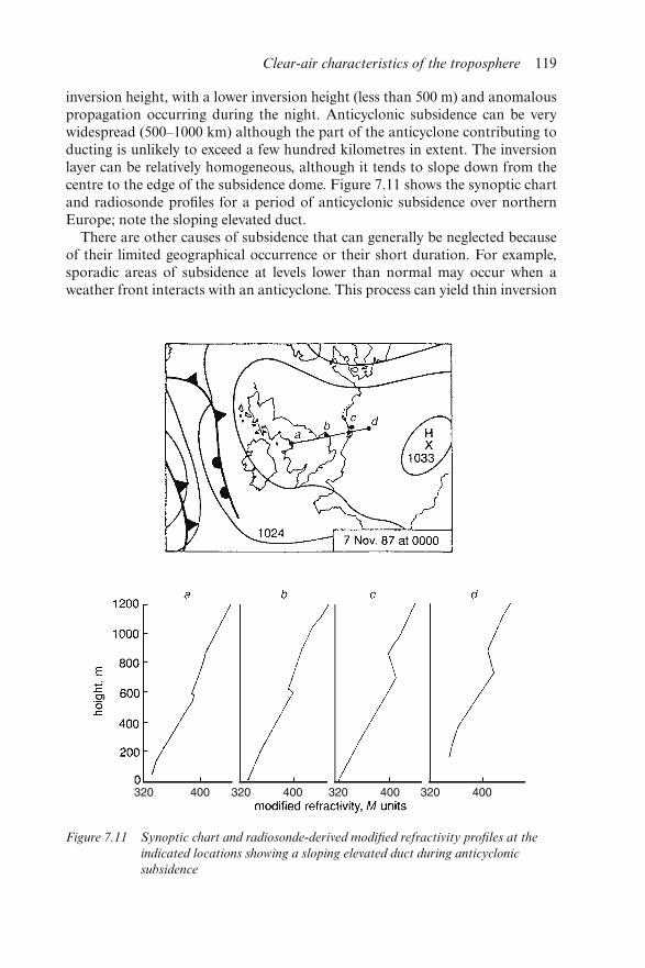
inversion height, with a lower inversion height (less than 500 m) and anomalouspropagation occurring during the night. Anticyclonic subsidence can be verywidespread (500–1000 km) although the part of the anticyclone contributing toducting is unlikely to exceed a few hundred kilometres in extent. The inversionlayer can be relatively homogeneous, although it tends to slope down from thecentre to the edge of the subsidence dome. Figure 7.11 shows the synoptic chartand radiosonde profiles for a period of anticyclonic subsidence over northernEurope; note the sloping elevated duct.
There are other causes of subsidence that can generally be neglected becauseof their limited geographical occurrence or their short duration. For example,sporadic areas of subsidence at levels lower than normal may occur when aweather front interacts with an anticyclone. This process can yield thin inversion
Figure 7.11 Synoptic chart and radiosonde-derived modified refractivity profiles at the
indicated locations showing a sloping elevated duct during anticyclonic
subsidence
Clear-air characteristics of the troposphere 119
layers with very strong gradients of humidity and temperature, and hence verysevere periods of anomalous propagation. This type of subsidence is short livedand localised, and appears more like a perturbation of the general anticyclonicpattern.
7.3.5 Advection
Advection ducts are of considerable importance in coastal regions such as theNorth Sea or enclosed seas with adjoining hot, dry land areas such as theMediterranean and the Gulf area. Advection is the large scale motion of airmasses. A duct can be formed when a warm, well mixed air mass flows off a landsurface over a cooler sea. In Northern Europe, advection is generally associatedwith anticyclonic subsidence: when a summer anticyclone is positioned overcontinental Europe, warm dry air is carried by advection from the continent outover the North Sea. The interaction of the continental air with the underlyingcooler, moister air just above the sea surface results in the formation of highhumidity lapse rates and temperature inversions, producing marked refractivitygradients. Advection ducts are usually surface based, typically less than 200 mthick. (Figure 7.9b shows an example.)
Whereas subsidence ducts are characterised by an almost trilinear shape, thetypical advection duct profile is smoother. As a result, these ducts are weakerand leakier than subsidence ducts. Nevertheless they constitute a major cause ofanomalous propagation in coastal areas as the surface duct couples strongly toterrestrial links and advection ducts tend to persist for several days at a time.Like subsidence, advection shows some diurnal variation, with a peak of activityexpected in the early evening. Advection ducts weaken away from the coast, butcan still be significant several hundred kilometres from it.
7.4 Propagation models
7.4.1 Statistical and deterministic models
Statistical models are often used for planning purposes to estimate the reliabilityof a system, or the level of interference to be expected to a service. They can bebased on the underlying physics of the problem, but because of a shortage orabsence of real-time input meteorological and other environmental data, andthe need for wide applicability and short computation times, these models tendto be semi-empirical, the model parameters being deduced from experimentaldata.
A different requirement arises when the operating environment of a system iswell characterised, the expense of obtaining real-time meteorological measure-ments is justified and there is a requirement to predict the performance of asystem in near real-time; this may include the need for a propagation forecasta day or two ahead. The performance of military surveillance radars and
120 Propagation of radiowaves
communication systems also comes into this category. Here a more completemodel based on physical principles is required.
We now describe the most important deterministic methods that have beenused to model radiowave propagation in clear-air conditions. Statistical modelsof clear-air propagation are described in Chapters 19 and 20.
7.4.2 Geometrical optics
Probably the simplest conceptual model for radiowave propagation is geo-metrical optics. When the medium changes slowly on the scale of a wavelength,the electromagnetic field is a plane wave locally, and the energy propagates alongrays which are trajectories orthogonal to the wavefronts. The rays are tracedoutwards from the transmitter, with the radius of curvature of the ray pathsdepending on the local refractive index gradients. Differential equations describ-ing the ray paths can be derived from repeated application of Snell’s law. Thesecan be integrated numerically in general, or in the case of one-dimensionalvertical refractive index profiles, can be integrated semi-analytically, yielding acomputationally efficient algorithm.
Figure 7.12 shows an example of ray tracing for a transmitter at 25 m heightin the presence of a simple elevated ducting layer. Ground reflected rays havebeen included. Note that the lower turning points of the ducted rays occur abovethe ground, typical of an elevated duct. There are several limitations of thisnaïve ray trace:
(a) when an individual ray encounters the layer it either penetrates it (such asthe ground reflected rays) or is turned round by it; there is no concept of aray splitting into two components (leakage out of the duct, partialreflection);
(b) the ray trace is frequency independent;(c) a single ray by itself carries no amplitude information.
The field strength can be derived from geometrical optics either by explicitlycalculating the cross section of a pencil of rays, or by integrating a further set ofdifferential equations – the transport equations. To calculate the field strength ata point, it is necessary to carefully categorise the rays into separate families (eachfamily containing rays that have followed similar trajectories), and to add coher-ently the contributions from all ray families passing through the point. Thiscoherent addition requires the phase of the field, obtained from the optical pathlength of the ray. Two-dimensional field plots based on these methods have beengenerated [15].
Apart from the difficulty of classifying rays into families automatically, thereis the problem that geometrical optics fails at ray caustics. A caustic is a locus ofpoints defining the boundary of a ray family. On one side of the caustic, two rayspass through each point, while on the other side there are no rays of that family.A caustic occurs between 60 and 80 km at a height of 20 m in Figure 7.12, andthere is a second caustic above this one at the boundary of the ray envelopes; the
Clear-air characteristics of the troposphere 121

two caustics meet at a point called a cusp. The ray equations predict infinite fieldstrength at caustics and cusps, with no energy reaching the region beyond acaustic from rays in the family giving rise to it. The problem is that geometricaloptics ignores the effects of diffraction. Unfortunately, these situations are likelyto arise in association with the anomalous refractive index structures that giverise to ducting. At long ranges in the presence of ducts many rays may linktransmitter and receiver and the number of caustics will build up with distancefrom the transmitter. In addition, the numerical accuracy required to calculatethe optical path lengths of these long rays is difficult to achieve, even if it isassumed that the refractive index along the path is sufficiently well characterisedfor stable results, which it rarely is in practice. If surface reflected rays arepresent, as in the case of a surface duct, the problem is compounded by thedifficulties of modelling the reflection, particularly if the surface is rough.
Although several sophisticated ray tracing programs are available which givegood qualitative results, and quantitative results in the shorter range, line-of-sight region, geometrical optics has severe difficulties for quantitativecalculations in the transhorizon region.
7.4.3 Mode theory
At ranges beyond a transmitter’s radio horizon, or in regions where the assump-tions of ray theory break down, field strength calculations can be made byfull wave methods. These attempt to find exact solutions (in principle) to Max-well’s equations for the given refractive index profile and transmitter–receivergeometry. For real situations, of course, such a solution is computationallyintractable, and approximating assumptions are inevitable.
Historically, a common approach was to impose strong constraints onthe representation of the measured refractive index profile. For example, if therefractive index is assumed to vary only in the vertical direction, the wave
Figure 7.12 Ray trace for a transmitter at 25 m height in the elevated duct shown
122 Propagation of radiowaves
equation can be separated and the imposition of matching conditions yieldsa one-dimensional equation, the mode equation. Even this one-dimensionalequation is difficult to solve in general; to simplify the problem, the profile wasoften approximated by simple shapes (such as linear segments) to which thereare standard solutions. Mode theory was first applied to tropospheric radio-wave propagation in Reference [16] and is fully described in Reference [17]; theapplication to elevated ducts was first given in Reference [18].
Mode theory in the troposphere is similar to mode propagation in a parallelplate waveguide. A duct of a given width will support a certain number ofpropagating (trapped) modes, the number being larger at higher frequencies.Higher-order modes are cut off and are evanescent. Each mode has an eigen-value and eigenfunction: the eigenvalue defines the phase velocity and attenu-ation rate of the mode; the eigenfunction is a height gain function that definesthe vertical distribution of energy in the mode. However, there is an importantdifference between tropospheric and waveguide modes: in the troposphere, atleast one of the duct boundaries is soft, as it is defined by a change in therefractive index gradient, rather than by a perfectly conducting plate. The con-sequence is that all tropospheric modes are leaky to some extent (that is, they areattenuated as they propagate) although the attenuation rate for the lowest-ordermodes may be very small. A physical picture of tropospheric modes is given inReference [19]; in particular Reference [19], Eqn. 9 shows that the total-internal-reflection criterion of geometrical optics given in Eqn. 7.13 is equivalent to thecondition for a mode to be well trapped. The field at a receiver is obtained bysumming the field contributions from all significant modes. Each contribution isa product of three terms: the height gain function evaluated at the transmitterheight, expressing the strength of coupling of the transmitter to the mode; theheight gain function evaluated at the receiver height; a term expressing theattenuation of the mode with range.
Mode theory has been successfully applied to long range propagation in theevaporation duct where there are a few, well trapped, modes and the transmitterand receiver are both strongly coupled into the duct. Mode theory becomesintractable at short range near the line of sight, and at high frequencies (or fordeep ducts) where the number of trapped modes becomes very large.
Although a one-dimensional approximation may be adequate for evaporationducts, it is inadequate for representing the meteorological structures which leadto elevated ducts. In general, horizontally homogeneous mode theory modelsoverestimate the path loss for terminals that are located outside a duct. Inhomo-geneities can give rise to higher field strengths due to mode mixing between thestrongly coupled, but leaky modes and the low loss, well trapped modes. Exten-sions of the theory to account for mode conversion in a stepped layer modelhave been made, but these are complex and there seems little future for thisapproach in practical prediction models. Another disadvantage of mode theoryis that there is no simple way of including the effects of terrain diffraction at theearth’s surface.
Clear-air characteristics of the troposphere 123
7.4.4 Parabolic equation
A more recent alternative to mode theory is the parabolic equation (PE) model[20–24]. Parabolic equation methods are described in some detail in Chapter 10,where they are applied to terrain diffraction. However, radiowave PE methodswere first developed for predicting the effects of atmospheric ducting over thesea. For this application, a two-dimensional split-step algorithm proved veryeffective and computationally efficient for calculating radar coverage diagrams/field strength contours on a personal computer. The method works at all ranges,thus avoiding the need for different models for the short and long distanceregimes. It also works equally well with real or complex refractive index, so theeffects of gaseous absorption (which can be variable from point to point) arevery easy to include within the PE framework. PE and hybrid ray PE models arenow incorporated in operational radar performance tools.
All the field contour plots in this Chapter were generated using the PE. Figure7.13 shows the PE results at three frequencies (3 GHz, 9.5 GHz and 18 GHz) forthe same refractive index profile as the ray trace of Figure 7.12, together with thestandard atmosphere picture at 9.5 GHz for reference. In the radar’s line-of-sight region the main feature is the interference lobing; the lobes are seen to bedistorted significantly by the presence of the layer. (Note that the lobes becomemore numerous at higher frequencies; in fact the number of lobes in a sector isproportional to h/λ where h is the antenna height and λ is the wavelength.) Asthe frequency increases, the pictures become more optical and begin to resemblethe ray trace as one would expect (compare Figures 7.13d and 7.12); note, how-ever, that the full-wave PE calculation contains much information missing fromthe ray trace: (a) the PE results are quantitative, and are frequency dependent;(b) leakage through the top of the layer is visible at all frequencies; at 3 GHz thefield is much more diffuse than the ray trace would suggest; (c) the PE solution isvalid at caustics and cusps, giving finite results. One of the principle advantagesof the PE method is its ability to handle two-dimensional refractive index data.Figure 7.14 shows the picture for the same case as Figure 7.13c, except that theducting layer has been assumed to weaken with range, returning to a standardatmosphere at 100 km (such as could occur in coastal advection). The secondlayer bounce at 90 km no longer occurs.
7.5 Turbulent scatter
In the troposphere small-scale irregularities in the propagation medium arecaused by small deviations of the temperature or humidity from the backgroundvalue. The process of creating these irregularities begins with the shear forcesbetween two moving air masses; this force creates large turbulent eddies at theouter scale of turbulence (typically 100 m). These large eddies spawn smallerand smaller eddies, transferring energy from the input range to smaller scalestructures in the transformation or inertial range. In fully developed turbulence,
124 Propagation of radiowaves
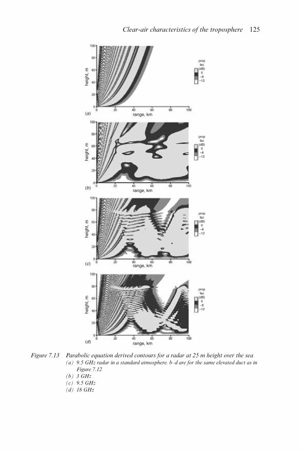
Figure 7.13 Parabolic equation derived contours for a radar at 25 m height over the sea(a) 9.5 GHz radar in a standard atmosphere. b–d are for the same elevated duct as in
Figure 7.12
(b) 3 GHz
(c) 9.5 GHz
(d) 18 GHz
Clear-air characteristics of the troposphere 125
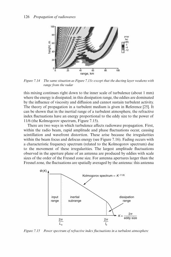
this mixing continues right down to the inner scale of turbulence (about 1 mm)where the energy is dissipated; in this dissipation range, the eddies are dominatedby the influence of viscosity and diffusion and cannot sustain turbulent activity.The theory of propagation in a turbulent medium is given in Reference [25]. Itcan be shown that in the inertial range of a turbulent atmosphere, the refractiveindex fluctuations have an energy proportional to the eddy size to the power of11/6 (the Kolmogorov spectrum, Figure 7.15).
There are two ways in which turbulence affects radiowave propagation. First,within the radio beam, rapid amplitude and phase fluctuations occur, causingscintillation and wavefront distortion. These arise because the irregularitieswithin the beam focus and defocus energy (see Figure 7.16). Fading occurs witha characteristic frequency spectrum (related to the Kolmogorov spectrum) dueto the movement of these irregularities. The largest amplitude fluctuationsobserved in the aperture plane of an antenna are produced by eddies with scalesizes of the order of the Fresnel zone size. For antenna apertures larger than theFresnel zone, the fluctuations are spatially averaged by the antenna: this antenna
Figure 7.14 The same situation as Figure 7.13c except that the ducting layer weakens with
range from the radar
Figure 7.15 Power spectrum of refractive index fluctuations in a turbulent atmosphere
126 Propagation of radiowaves
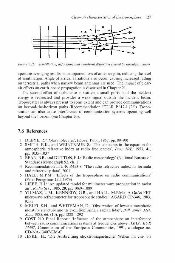
aperture averaging results in an apparent loss of antenna gain, reducing the levelof scintillation. Angle of arrival variations also occur, causing increased fadingon terrestrial paths when narrow beam antennas are used. The impact of clear-air effects on earth–space propagation is discussed in Chapter 21.
The second effect of turbulence is scatter: a small portion of the incidentenergy is redirected and provides a weak signal outside the incident beam.Troposcatter is always present to some extent and can provide communicationson beyond-the-horizon paths (Recommendation ITU-R P.617-1 [26]). Tropo-scatter can also cause interference to communication systems operating wellbeyond the horizon (see Chapter 20).
7.6 References
1 DEBYE, P.: ‘Polar molecules’, (Dover Publ., 1957, pp. 89–90)2 SMITH, E.K., and WEINTRAUB, S.: ‘The constants in the equation for
atmospheric refractive index at radio frequencies’, Proc. IRE, 1953, 41,pp. 1035–1037
3 BEAN, B.R. and DUTTON, E.J.: ‘Radio meteorology’ (National Bureau ofStandards Monograph 92, ch. 1)
4 Recommendation ITU-R P.453-8: ‘The radio refractive index: its formulaand refractivity data’, 2001
5 HALL, M.P.M.: ‘Effects of the troposphere on radio communications’(Peter Peregrinus Ltd, 1979)
6 LIEBE, H.J.: ‘An updated model for millimeter wave propagation in moistair’, Radio Sci., 1985, 20, pp. 1069–1089
7 YILMAZ, U.M., KENNEDY, G.R., and HALL, M.P.M.: ‘A GaAs FETmicrowave refractometer for tropospheric studies’. AGARD CP-346, 1983,9.1-5
8 MELFI, S.H., and WHITEMAN, D.: ‘Observation of lower-atmosphericmoisture structure and its evolution using a raman lidar’, Bull. Amer. Met.Soc., 1985, 66, (10), pp. 1288–1292
9 COST 210 Final Report: ‘Influence of the atmosphere on interferencebetween radio communications systems at frequencies above 1GHz’. EUR13407, Commission of the European Communities, 1991, catalogue no.CD-NA-13407-EM-C
10 JESKE, H.: ‘Die Ausbreitung elecktromagnetischer Wellen im cm- bis
Figure 7.16 Scintillation, defocusing and wavefront distortion caused by turbulent scatter
Clear-air characteristics of the troposphere 127
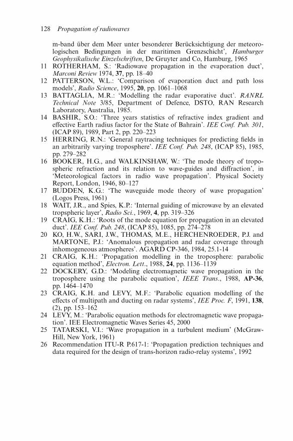
m-band über dem Meer unter besonderer Berücksichtigung der meteoro-logischen Bedingungen in der maritimen Grenzschicht’, HamburgerGeophysikalische Einzelschriften, De Gruyter and Co, Hamburg, 1965
11 ROTHERHAM, S.: ‘Radiowave propagation in the evaporation duct’,Marconi Review 1974, 37, pp. 18–40
12 PATTERSON, W.L.: ‘Comparison of evaporation duct and path lossmodels’, Radio Science, 1995, 20, pp. 1061–1068
13 BATTAGLIA, M.R.: ‘Modelling the radar evaporative duct’. RANRLTechnical Note 3/85, Department of Defence, DSTO, RAN ResearchLaboratory, Australia, 1985.
14 BASHIR, S.O.: ‘Three years statistics of refractive index gradient andeffective Earth radius factor for the State of Bahrain’. IEE Conf. Pub. 301,(ICAP 89), 1989, Part 2, pp. 220–223
15 HERRING, R.N.: ‘General raytracing techniques for predicting fields inan arbitrarily varying troposphere’. IEE Conf. Pub. 248, (ICAP 85), 1985,pp. 279–282
16 BOOKER, H.G., and WALKINSHAW, W.: ‘The mode theory of tropo-spheric refraction and its relation to wave-guides and diffraction’, in‘Meteorological factors in radio wave propagation’. Physical SocietyReport, London, 1946, 80–127
17 BUDDEN, K.G.: ‘The waveguide mode theory of wave propagation’(Logos Press, 1961)
18 WAIT, J.R., and Spies, K.P.: ‘Internal guiding of microwave by an elevatedtropspheric layer’, Radio Sci., 1969, 4, pp. 319–326
19 CRAIG, K.H.: ‘Roots of the mode equation for propagation in an elevatedduct’. IEE Conf. Pub. 248, (ICAP 85), 1085, pp. 274–278
20 KO, H.W., SARI, J.W., THOMAS, M.E., HERCHENROEDER, P.J. andMARTONE, P.J.: ‘Anomalous propagation and radar coverage throughinhomogeneous atmospheres’. AGARD CP-346, 1984, 25.1-14
21 CRAIG, K.H.: ‘Propagation modelling in the troposphere: parabolicequation method’, Electron. Lett., 1988, 24, pp. 1136–1139
22 DOCKERY, G.D.: ‘Modeling electromagnetic wave propagation in thetroposphere using the parabolic equation’, IEEE Trans., 1988, AP-36,pp. 1464–1470
23 CRAIG, K.H. and LEVY, M.F.: ‘Parabolic equation modelling of theeffects of multipath and ducting on radar systems’, IEE Proc. F, 1991, 138,(2), pp. 153–162
24 LEVY, M.: ‘Parabolic equation methods for electromagnetic wave propaga-tion’. IEE Electromagnetic Waves Series 45, 2000
25 TATARSKI, V.I.: ‘Wave propagation in a turbulent medium’ (McGraw-Hill, New York, 1961)
26 Recommendation ITU-R P.617-1: ‘Propagation prediction techniques anddata required for the design of trans-horizon radio-relay systems’, 1992
128 Propagation of radiowaves
Chapter 8
Introduction to diffraction
David Bacon
8.1 Underlying principles
Diffraction can be treated as a highly theoretical subject, although the under-lying process can be visualised quite readily. It is usually interpreted in terms ofthe wave nature of electromagnetic radiation, although there is an argument thatquantum uncertainty provides a better physical description. Whatever the case,this Chapter will use the concept of radiowaves to describe the cause and effectsof diffraction.
8.1.1 Signal variations at the edge of a radio shadow
Radio energy does not simply travel in straight lines. As an example, Figure 8.1shows the variation of illumination at the edge of a radio shadow. On the left aplane radio wavefront travelling to the right is obstructed up to a certain heightby a thin totally absorbing obstruction. The graph on the right shows the vari-ation of signal level in dB (horizontal scale) against height (vertical scale) at apoint beyond the obstruction.
In Figure 8.1 the dB scale is relative to the signal level that would exist ifthe obstruction were absent; it is clearly not the sharp-edged shadow we are usedto with light. Just above the obstruction the signal level oscillates; at the edge ofthe physical obstruction the signal is at −6 dB, not the half-power value of −3 dBas might be assumed, and the signal level does not immediately fall to zerobehind the obstruction.
However, exactly the same pattern does in fact exist with light, it is just toosmall to see under normal circumstances. Due to the much longer wavelengths,the patterns which exist at radio frequencies can be large and highlysignificant.
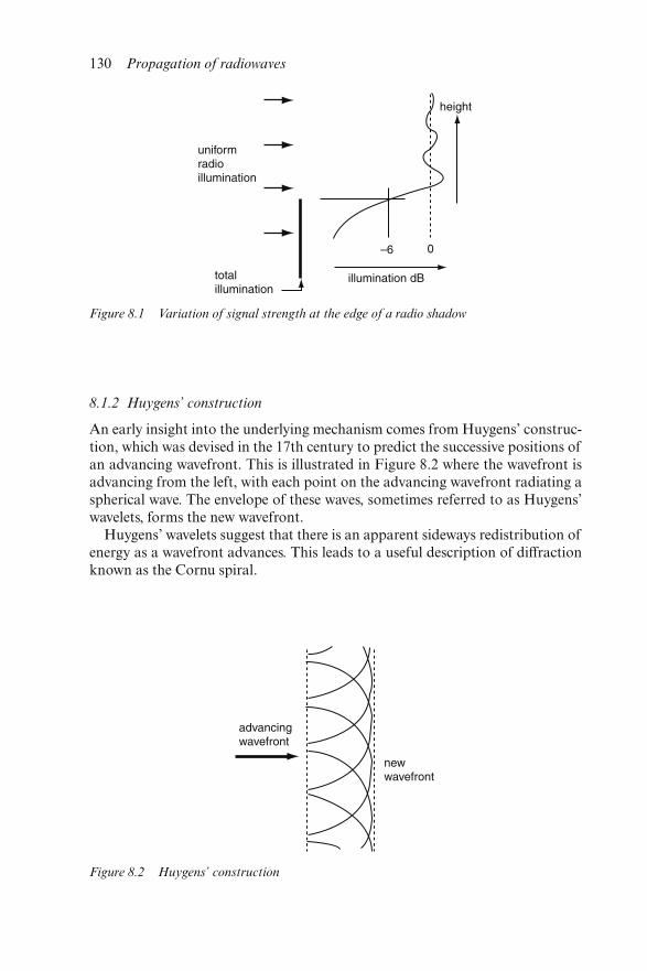
8.1.2 Huygens’ construction
An early insight into the underlying mechanism comes from Huygens’ construc-tion, which was devised in the 17th century to predict the successive positions ofan advancing wavefront. This is illustrated in Figure 8.2 where the wavefront isadvancing from the left, with each point on the advancing wavefront radiating aspherical wave. The envelope of these waves, sometimes referred to as Huygens’wavelets, forms the new wavefront.
Huygens’ wavelets suggest that there is an apparent sideways redistribution ofenergy as a wavefront advances. This leads to a useful description of diffractionknown as the Cornu spiral.
Figure 8.1 Variation of signal strength at the edge of a radio shadow
Figure 8.2 Huygens’ construction
130 Propagation of radiowaves
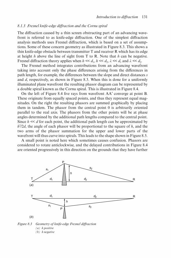
8.1.3 Fresnel knife-edge diffraction and the Cornu spiral
The diffraction caused by a thin screen obstructing part of an advancing wave-front is referred to as knife-edge diffraction. One of the simplest diffractionanalysis methods uses Fresnel diffraction, which is based on a set of assump-tions. Some of these concern geometry as illustrated in Figure 8.3. This shows athin knife-edge obstacle between transmitter T and receiver R which has its edgeat height h above the line of sight from T to R. Note that h can be negative.Fresnel diffraction theory applies when h << d1, h << d2, λ << d1 and λ << d2.
The Fresnel method integrates contributions from an advancing wavefronttaking into account only the phase differences arising from the differences inpath length, for example, the differences between the slope and direct distances sand d, respectively, as shown in Figure 8.3. When this is done for a uniformlyilluminated plane wavefront the resulting phasor diagram can be represented bya double spiral known as the Cornu spiral. This is illustrated in Figure 8.4.
On the left of Figure 8.4 five rays from wavefront AA′ converge at point B.These originate from equally spaced points, and thus they represent equal mag-nitudes. On the right the resulting phasors are summed graphically by placingthem in tandem. The phasor from the central point 0 is arbitrarily orientedparallel to the real axis. The phasors from the other points will be at phaseangles determined by the additional path lengths compared to the central point.Since h << d for each point, the additional path length can be approximated byh2/2d, the angle of each phasor will be proportional to the square of h, and thetwo arms of the phasor summation for the upper and lower parts of thewavefront will thus curve into spirals. This leads to the shape shown in Figure 8.5.
A small point is noted here which sometimes causes confusion. Phasors areconsidered to rotate anticlockwise, and the delayed contributions in Figure 8.4are oriented progressively in this direction on the grounds that they have further
Figure 8.3 Geometry of knife-edge Fresnel diffraction(a) h positive
(b) h negative
Introduction to diffraction 131
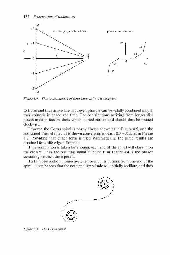
to travel and thus arrive late. However, phasors can be validly combined only ifthey coincide in space and time. The contributions arriving from longer dis-tances must in fact be those which started earlier, and should thus be rotatedclockwise.
However, the Cornu spiral is nearly always shown as in Figure 8.5, and theassociated Fresnel integral is shown converging towards 0.5 + j0.5, as in Figure8.7. Providing that either form is used systematically, the same results areobtained for knife-edge diffraction.
If the summation is taken far enough, each end of the spiral will close in onthe crosses. Thus the resulting signal at point B in Figure 8.4 is the phasorextending between these points.
If a thin obstruction progressively removes contributions from one end of thespiral, it can be seen that the net signal amplitude will initially oscillate, and then
Figure 8.4 Phasor summation of contributions from a wavefront
Figure 8.5 The Cornu spiral
132 Propagation of radiowaves
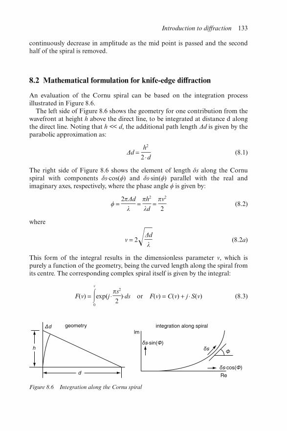
continuously decrease in amplitude as the mid point is passed and the secondhalf of the spiral is removed.
8.2 Mathematical formulation for knife-edge diffraction
An evaluation of the Cornu spiral can be based on the integration processillustrated in Figure 8.6.
The left side of Figure 8.6 shows the geometry for one contribution from thewavefront at height h above the direct line, to be integrated at distance d alongthe direct line. Noting that h << d, the additional path length Δd is given by theparabolic approximation as:
Δd = h2
2 ⋅d(8.1)
The right side of Figure 8.6 shows the element of length δs along the Cornuspiral with components δs⋅cos() and δs⋅sin() parallel with the real andimaginary axes, respectively, where the phase angle is given by:
= 2πΔd
λ =
πh2
λd =
πν2
2(8.2)
where
ν = 2�Δd
λ(8.2a)
This form of the integral results in the dimensionless parameter ν, which ispurely a function of the geometry, being the curved length along the spiral fromits centre. The corresponding complex spiral itself is given by the integral:
F(ν) = �ν
0
exp(j ⋅πs2
2)⋅ds or F(ν) = C(ν) + j ⋅S(ν) (8.3)
Figure 8.6 Integration along the Cornu spiral
Introduction to diffraction 133
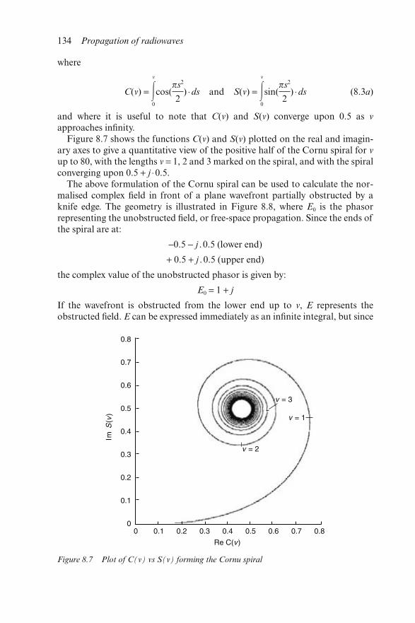
where
C(ν) = �ν
0
cos(πs2
2) ⋅ds and S(ν) = �
ν
0
sin(πs2
2) ⋅ds (8.3a)
and where it is useful to note that C(ν) and S(ν) converge upon 0.5 as ν
approaches infinity.Figure 8.7 shows the functions C(ν) and S(ν) plotted on the real and imagin-
ary axes to give a quantitative view of the positive half of the Cornu spiral for νup to 80, with the lengths ν = 1, 2 and 3 marked on the spiral, and with the spiralconverging upon 0.5 + j ⋅0.5.
The above formulation of the Cornu spiral can be used to calculate the nor-malised complex field in front of a plane wavefront partially obstructed by aknife edge. The geometry is illustrated in Figure 8.8, where E0 is the phasorrepresenting the unobstructed field, or free-space propagation. Since the ends ofthe spiral are at:
−0.5 − j . 0.5 (lower end)
+ 0.5 + j . 0.5 (upper end)
the complex value of the unobstructed phasor is given by:
E0 = 1 + j
If the wavefront is obstructed from the lower end up to ν, E represents theobstructed field. E can be expressed immediately as an infinite integral, but since
Figure 8.7 Plot of C(ν) vs S(ν) forming the Cornu spiral
134 Propagation of radiowaves
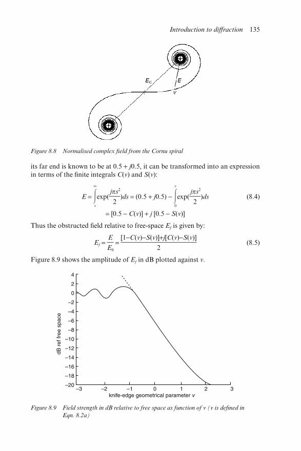
its far end is known to be at 0.5 + j0.5, it can be transformed into an expressionin terms of the finite integrals C(ν) and S(ν):
E = �∞
ν
exp(jπs2
2)ds = (0.5 + j0.5) − �
ν
0
exp(jπs2
2)ds (8.4)
= [0.5 − C(ν)] + j [0.5 − S(ν)]
Thus the obstructed field relative to free-space Ef is given by:
Ef = E
E0
= [1−C(ν)−S(ν)]+j[C(ν)−S(ν)]
2(8.5)
Figure 8.9 shows the amplitude of Ef in dB plotted against ν.
Figure 8.8 Normalised complex field from the Cornu spiral
Figure 8.9 Field strength in dB relative to free space as function of ν (ν is defined in
Eqn. 8.2a)
Introduction to diffraction 135
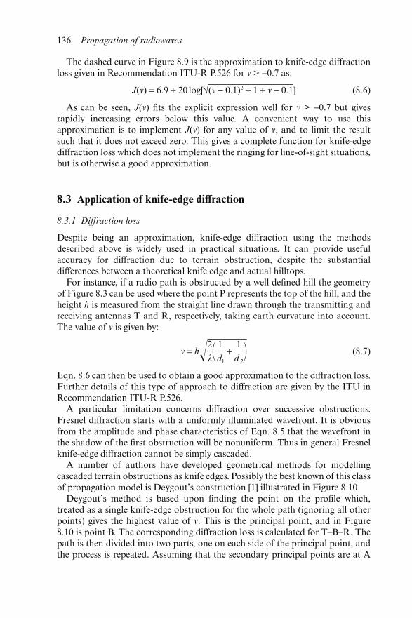
The dashed curve in Figure 8.9 is the approximation to knife-edge diffractionloss given in Recommendation ITU-R P.526 for ν > −0.7 as:
J(ν) = 6.9 + 20 log[√(ν − 0.1)2 + 1 + ν − 0.1] (8.6)
As can be seen, J(ν) fits the explicit expression well for ν > −0.7 but givesrapidly increasing errors below this value. A convenient way to use thisapproximation is to implement J(ν) for any value of ν, and to limit the resultsuch that it does not exceed zero. This gives a complete function for knife-edgediffraction loss which does not implement the ringing for line-of-sight situations,but is otherwise a good approximation.
8.3 Application of knife-edge diffraction
8.3.1 Diffraction loss
Despite being an approximation, knife-edge diffraction using the methodsdescribed above is widely used in practical situations. It can provide usefulaccuracy for diffraction due to terrain obstruction, despite the substantialdifferences between a theoretical knife edge and actual hilltops.
For instance, if a radio path is obstructed by a well defined hill the geometryof Figure 8.3 can be used where the point P represents the top of the hill, and theheight h is measured from the straight line drawn through the transmitting andreceiving antennas T and R, respectively, taking earth curvature into account.The value of ν is given by:
ν = h�2
λ�1
d1
+ 1
d 2� (8.7)
Eqn. 8.6 can then be used to obtain a good approximation to the diffraction loss.Further details of this type of approach to diffraction are given by the ITU inRecommendation ITU-R P.526.
A particular limitation concerns diffraction over successive obstructions.Fresnel diffraction starts with a uniformly illuminated wavefront. It is obviousfrom the amplitude and phase characteristics of Eqn. 8.5 that the wavefront inthe shadow of the first obstruction will be nonuniform. Thus in general Fresnelknife-edge diffraction cannot be simply cascaded.
A number of authors have developed geometrical methods for modellingcascaded terrain obstructions as knife edges. Possibly the best known of this classof propagation model is Deygout’s construction [1] illustrated in Figure 8.10.
Deygout’s method is based upon finding the point on the profile which,treated as a single knife-edge obstruction for the whole path (ignoring all otherpoints) gives the highest value of ν. This is the principal point, and in Figure8.10 is point B. The corresponding diffraction loss is calculated for T–B–R. Thepath is then divided into two parts, one on each side of the principal point, andthe process is repeated. Assuming that the secondary principal points are at A
136 Propagation of radiowaves
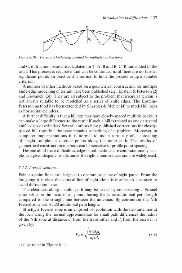
and C, diffraction losses are calculated for T–A–B and B–C–R and added to thetotal. This process is recursive, and can be continued until there are no furthersignificant points. In practice it is normal to limit the process using a suitablecriterion.
A number of other methods based on a geometrical construction for multipleknife-edge modelling of terrain have been published (e.g., Epstein & Peterson [2]and Giovanelli [3]). They are all subject to the problem that irregular terrain isnot always suitable to be modelled as a series of knife edges. The Epstein–Peterson method has been extended by Sharples & Mehler [4] to model hill topsas horizontal cylinders.
A further difficulty is that a hill top may have closely-spaced multiple peaks; itcan make a large difference to the result if such a hill is treated as one or severalknife edges or cylinders. Several authors have published corrections for closely-spaced hill tops, but the issue remains something of a problem. Moreover, incomputer implementations it is normal to use a terrain profile consistingof height samples at discrete points along the radio path. The results ofgeometrical construction methods can be sensitive to profile point spacing.
Despite all of these difficulties, edge-based methods are computationally sim-ple, can give adequate results under the right circumstances and are widely used.
8.3.2 Fresnel clearance
Point-to-point links are designed to operate over line-of-sight paths. From theforegoing it is clear that optical line of sight alone is insufficient clearance toavoid diffraction losses.
The clearance along a radio path may be tested by constructing a Fresnelzone, which is the locus of all points having the same additional path lengthcompared to the straight line between the antennas. By convention the NthFresnel zone has N .λ/2 additional path length.
Strictly, a Fresnel zone is an ellipsoid of revolution with the two antennas atthe foci. Using the normal approximation for small path differences the radiusof the Nth zone at distance d1 from the transmitter and d2 from the receiver isgiven by:
FN = �Nλd1d2
d1+d2
(8.8)
as illustrated in Figure 8.11.
Figure 8.10 Deygout’s knife-edge method for multiple obstructions
Introduction to diffraction 137
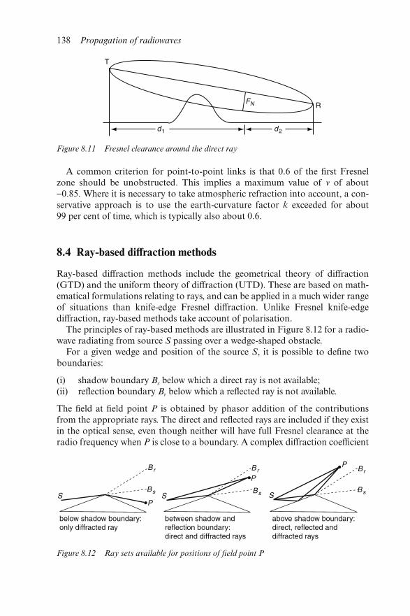
A common criterion for point-to-point links is that 0.6 of the first Fresnelzone should be unobstructed. This implies a maximum value of ν of about−0.85. Where it is necessary to take atmospheric refraction into account, a con-servative approach is to use the earth-curvature factor k exceeded for about99 per cent of time, which is typically also about 0.6.
8.4 Ray-based diffraction methods
Ray-based diffraction methods include the geometrical theory of diffraction(GTD) and the uniform theory of diffraction (UTD). These are based on math-ematical formulations relating to rays, and can be applied in a much wider rangeof situations than knife-edge Fresnel diffraction. Unlike Fresnel knife-edgediffraction, ray-based methods take account of polarisation.
The principles of ray-based methods are illustrated in Figure 8.12 for a radio-wave radiating from source S passing over a wedge-shaped obstacle.
For a given wedge and position of the source S, it is possible to define twoboundaries:
(i) shadow boundary Bs below which a direct ray is not available;(ii) reflection boundary Br below which a reflected ray is not available.
The field at field point P is obtained by phasor addition of the contributionsfrom the appropriate rays. The direct and reflected rays are included if they existin the optical sense, even though neither will have full Fresnel clearance at theradio frequency when P is close to a boundary. A complex diffraction coefficient
Figure 8.11 Fresnel clearance around the direct ray
Figure 8.12 Ray sets available for positions of field point P
138 Propagation of radiowaves
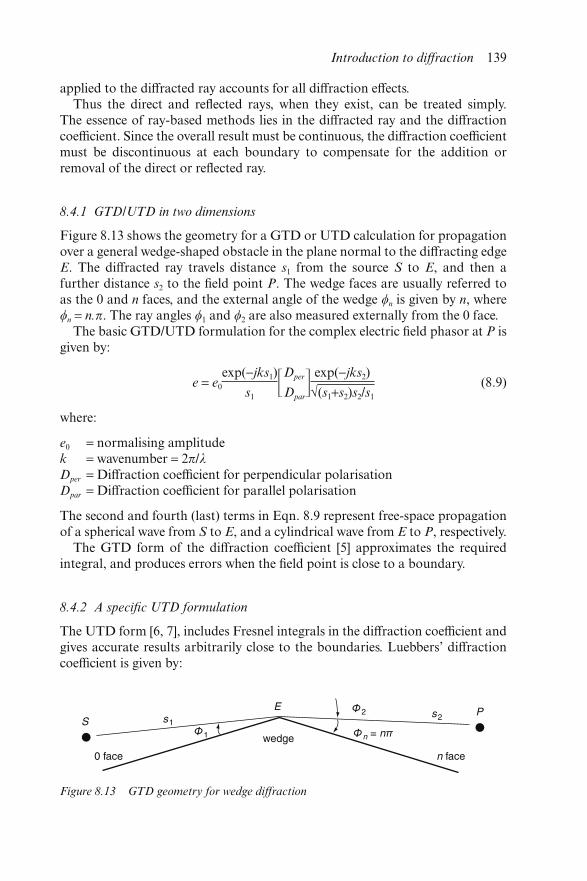
applied to the diffracted ray accounts for all diffraction effects.Thus the direct and reflected rays, when they exist, can be treated simply.
The essence of ray-based methods lies in the diffracted ray and the diffractioncoefficient. Since the overall result must be continuous, the diffraction coefficientmust be discontinuous at each boundary to compensate for the addition orremoval of the direct or reflected ray.
8.4.1 GTD/UTD in two dimensions
Figure 8.13 shows the geometry for a GTD or UTD calculation for propagationover a general wedge-shaped obstacle in the plane normal to the diffracting edgeE. The diffracted ray travels distance s1 from the source S to E, and then afurther distance s2 to the field point P. The wedge faces are usually referred toas the 0 and n faces, and the external angle of the wedge n is given by n, wheren = n.π. The ray angles 1 and 2 are also measured externally from the 0 face.
The basic GTD/UTD formulation for the complex electric field phasor at P isgiven by:
e = e0
exp(−jks1)
s1Dper
Dpar� exp(−jks2)
√(s1+s2)s2/s1
(8.9)
where:
e0 = normalising amplitudek = wavenumber = 2π/λDper = Diffraction coefficient for perpendicular polarisationDpar = Diffraction coefficient for parallel polarisation
The second and fourth (last) terms in Eqn. 8.9 represent free-space propagationof a spherical wave from S to E, and a cylindrical wave from E to P, respectively.
The GTD form of the diffraction coefficient [5] approximates the requiredintegral, and produces errors when the field point is close to a boundary.
8.4.2 A specific UTD formulation
The UTD form [6, 7], includes Fresnel integrals in the diffraction coefficient andgives accurate results arbitrarily close to the boundaries. Luebbers’ diffractioncoefficient is given by:
Figure 8.13 GTD geometry for wedge diffraction
Introduction to diffraction 139
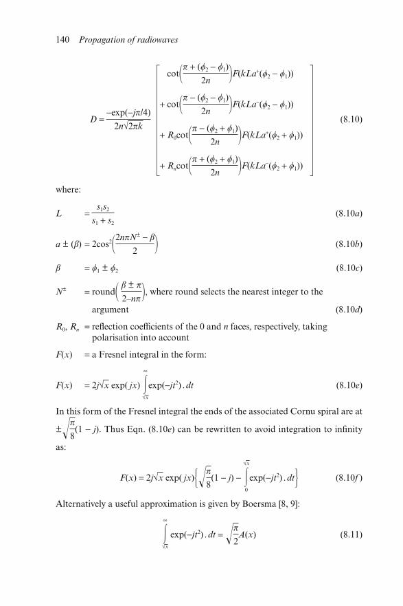
D =−exp(−jπ/4)
2n√2πk
cot�π + (2 − 1)
2n �F(kLa+(2 − 1))
(8.10)
+ cot�π − (2 − 1)
2n �F(kLa−(2 − 1))
+ R0cot�π − (2 + 1)
2n �F(kLa+(2 + 1))
+ Rncot�π + (2 + 1)
2n �F(kLa−(2 + 1))
where:
L = s1s2
s1 + s2
(8.10a)
a ± (β) = 2cos2�2nπN± − β
2 � (8.10b)
β = 1 ± 2 (8.10c)
N± = round� β ± π
2–nπ�, where round selects the nearest integer to the
argument (8.10d)
R0, Rn = reflection coefficients of the 0 and n faces, respectively, taking polarisation into account
F(x) = a Fresnel integral in the form:
F(x) = 2j√x exp( jx) �∞
√x
exp(−jt2) .dt (8.10e)
In this form of the Fresnel integral the ends of the associated Cornu spiral are at
±�π
8(1 − j). Thus Eqn. (8.10e) can be rewritten to avoid integration to infinity
as:
F(x) = 2j√x exp( jx)��π
8(1 − j) − �
√x
0
exp(−jt2) .dt� (8.10f )
Alternatively a useful approximation is given by Boersma [8, 9]:
�∞
√x
exp(−jt2) .dt = �π
2A(x) (8.11)
140 Propagation of radiowaves
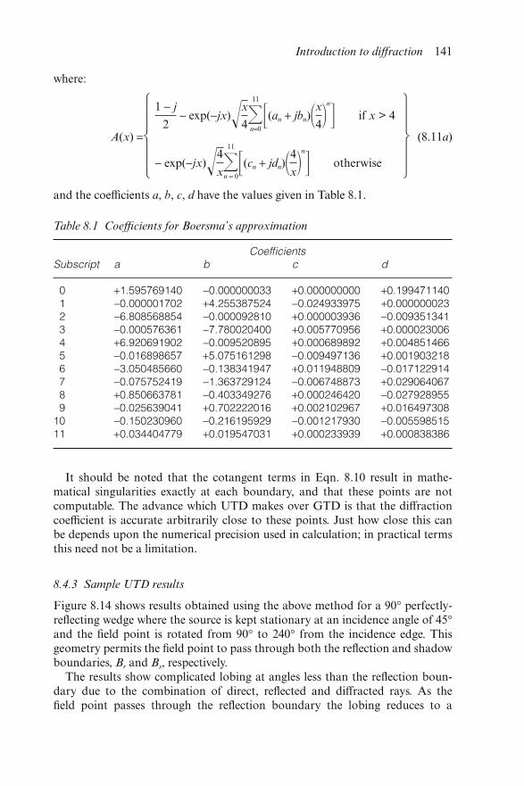
where:
A(x) =
1 − j
2 − exp(−jx)�x
4�11
n=0(an + jbn)�x4�
n
� if x > 4
(8.11a)
− exp(−jx)�4
x�
11
n = 0(cn + jdn)�4
x�n
� otherwise
⎧ ⎫⎪ ⎪⎭ ⎩⎫ ⎧⎪ ⎪⎩ ⎭
and the coefficients a, b, c, d have the values given in Table 8.1.
It should be noted that the cotangent terms in Eqn. 8.10 result in mathe-matical singularities exactly at each boundary, and that these points are notcomputable. The advance which UTD makes over GTD is that the diffractioncoefficient is accurate arbitrarily close to these points. Just how close this canbe depends upon the numerical precision used in calculation; in practical termsthis need not be a limitation.
8.4.3 Sample UTD results
Figure 8.14 shows results obtained using the above method for a 90° perfectly-reflecting wedge where the source is kept stationary at an incidence angle of 45°and the field point is rotated from 90° to 240° from the incidence edge. Thisgeometry permits the field point to pass through both the reflection and shadowboundaries, Br and Bs, respectively.
The results show complicated lobing at angles less than the reflection boun-dary due to the combination of direct, reflected and diffracted rays. As thefield point passes through the reflection boundary the lobing reduces to a
Table 8.1 Coefficients for Boersma’s approximation
CoefficientsSubscript a b c d
0 +1.595769140 −0.000000033 +0.000000000 +0.1994711401 −0.000001702 +4.255387524 −0.024933975 +0.0000000232 −6.808568854 −0.000092810 +0.000003936 −0.0093513413 −0.000576361 −7.780020400 +0.005770956 +0.0000230064 +6.920691902 −0.009520895 +0.000689892 +0.0048514665 −0.016898657 +5.075161298 −0.009497136 +0.0019032186 −3.050485660 −0.138341947 +0.011948809 −0.0171229147 −0.075752419 −1.363729124 −0.006748873 +0.0290640678 +0.850663781 −0.403349276 +0.000246420 −0.0279289559 −0.025639041 +0.702222016 +0.002102967 +0.016497308
10 −0.150230960 −0.216195929 −0.001217930 −0.00559851511 +0.034404779 +0.019547031 +0.000233939 +0.000838386
Introduction to diffraction 141
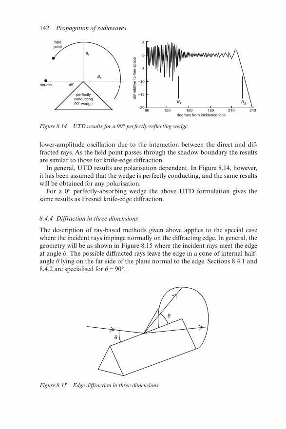
lower-amplitude oscillation due to the interaction between the direct and dif-fracted rays. As the field point passes through the shadow boundary the resultsare similar to those for knife-edge diffraction.
In general, UTD results are polarisation dependent. In Figure 8.14, however,it has been assumed that the wedge is perfectly conducting, and the same resultswill be obtained for any polarisation.
For a 0° perfectly-absorbing wedge the above UTD formulation gives thesame results as Fresnel knife-edge diffraction.
8.4.4 Diffraction in three dimensions
The description of ray-based methods given above applies to the special casewhere the incident rays impinge normally on the diffracting edge. In general, thegeometry will be as shown in Figure 8.15 where the incident rays meet the edgeat angle θ. The possible diffracted rays leave the edge in a cone of internal half-angle θ lying on the far side of the plane normal to the edge. Sections 8.4.1 and8.4.2 are specialised for θ = 90°.
Figure 8.14 UTD results for a 90° perfectly-reflecting wedge
Figure 8.15 Edge diffraction in three dimensions
142 Propagation of radiowaves
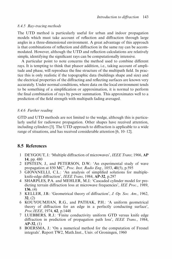
8.4.5 Ray-tracing methods
The UTD method is particularly useful for urban and indoor propagationmodels which must take account of reflection and diffraction through largeangles in a three-dimensional environment. A great advantage of this approachis that combinations of reflection and diffraction in the same ray can be accom-modated. However, although the UTD and reflection calculations are relativelysimple, identifying the significant rays can be computationally intensive.
A particular point to note concerns the method used to combine differentrays. It is tempting to think that phasor addition, i.e., taking account of ampli-tude and phase, will reproduce the fine structure of the multipath field. In prac-tice this is only realistic if the topographic data (buildings shape and size) andthe electrical properties of the diffracting and reflecting surfaces are known veryaccurately. Under normal conditions, where data on the local environment tendsto be something of a simplification or approximation, it is normal to performthe final combination of rays by power summation. This approximates well to aprediction of the field strength with multipath fading averaged.
8.4.6 Further reading
GTD and UTD methods are not limited to the wedge, although this is particu-larly useful for radiowave propagation. Other shapes have received attention,including cylinders [3]. The UTD approach to diffraction is applicable to a widerange of situations, and has received considerable attention [6, 10–12].
8.5 References
1 DEYGOUT, J.: ‘Multiple diffraction of microwaves’, IEEE Trans; 1966, AP14, pp. 480
2 EPSTEIN, J., and PETERSON, D.W.: ‘An experimental study of wavepropagation at 850 MC’, Proc. Inst. Radio Eng., 1053, 41(5), p.595
3 GIOVANELLI, C.L.: ‘An analysis of simplified solutions for multiple-knife-edge diffraction’, IEEE Trans, 1984, AP-32, p.297
4 SHARPLES, P.A. and MEHLER, M.J.: ‘Cascaded cylinder model for pre-dicting terrain diffraction loss at microwave frequencies’, IEE Proc., 1989,136, (4)
5 KELLER, J.B.: ‘Geometrical theory of diffraction’, J. Op. Soc. Am., 1962,32, (2)
6 KOUYOUMJIAN, R.G., and PATHAK, P.H.: ‘A uniform geometricaltheory of diffraction for an edge in a perfectly conducting surface’,Proc.IEEE, 1974, 62, p.1448
7 LUEBBERS, R.J.: ‘Finite conductivity uniform GTD versus knife edgediffraction in prediction of propagation path loss’, IEEE Trans., 1984,AP-32, (1)
8 BOERSMA, J.: ‘On a numerical method for the computation of Fresnelintegrals’. Report TW2, Math.Inst., Univ. of Groningen, 1960
Introduction to diffraction 143

9 BOERSMA, J.: ‘Computation of Fresnel integrals’, J.Math.Comput., 1960,14, p.380
10 VOGLER, L.E.: ‘An attenuation factor for multiple knife edge diffraction’,Radio Sci, 1982, 17, (6)
11 DEMETRESCU, C.: ‘A general solution of the second-order differenceequation occurring in diffraction theory’, Radio Sci., 1996, 31, (3)
12 DEMETRESCU, C., et al.: ‘TM electromagnetic scattering by a trans-parent wedge with resistive faces’ IEEE Trans. 1999, AP-47, (1)
144 Propagation of radiowaves
Chapter 9
Short-range propagation
Les Barclay
9.1 Introduction
Short-range radio systems are used for many purposes – for telemetry, remotecontrol and games, as well as for communications. Communications uses includecordless telephony, radio local area networks (RLANs), radio fixed access andmicrocellular systems.
For some of these applications very low powers are used with poor andpoorly located antennas where the user only expects the range to be of theorder of a few metres. For example, for remote car door locks, the userwill expect to point the transmitter towards the car and probably has someunderstanding of the need to provide a near line-of-sight path. For such appli-cations there seems to be very little requirement to attempt to provide goodpropagation models.
For RLANs and other indoor applications there will be a need for some kindof generic modelling of the effects of the room size and shape, obstructions inthe room, the construction materials and the penetration through walls andfloors. For high-speed data transmission it may also be necessary to model themultipath time spreads.
But for outdoor microcellular systems and similar applications it will benecessary to model propagation at distances ranging out to a kilometre or so,where the longer-range area coverage prediction methods may take over. 1 km isthe dividing distance used by the ITU-R in its Recommendations betweenshort-range and longer-range prediction methods.
However, the above considerations mainly apply to VHF and UHF systems,where although the distances are short the propagation is in the far field regimeand the usual propagation techniques are applicable. Another interpretation ofshort range would be to consider paths within the near field regime around thetransmitting antenna. This is mainly of significance at lower frequencies.

It is also useful to include a discussion of propagation in tunnels and otherrestricted areas.
9.2 Outdoor propagation
9.2.1 Outdoor path categories
This Section presents the methods outlined in Recommendation ITU-R P.1411,and is restricted to a discussion of methods applicable to ranges up to 1 km. Themethods may extend to somewhat longer ranges, see Chapter 11.
Account should be taken of the details of the environment and of the serviceapplication. Tables 9.1 to 9.3 summarise the factors to be considered.
Various propagation environments can be envisaged for short range outdoorpropagation in urban areas.
Table 9.1 Physical operating environments
Environment Description and propagation impairments of concern
Urban high-rise • urban canyon, characterised by streets lined withtall buildings of several floors each
• building height makes significant contributionsfrom propagation over rooftops unlikely
• rows of tall buildings provide the possibility of longpath delays
• large numbers of moving vehicles in the area act asreflectors adding Doppler shift to the reflectedwaves
Urban/suburban low-rise • typified by wide streets• building heights are generally less than three
stories making diffraction over rooftop likely• reflections and shadowing from moving vehicles
can occur• primary effects are long delays and small Doppler
shiftsResidential • single and double story dwellings
• roads are generally two lanes wide with carsparked along sides
• heavy to light foliage possible• motor traffic usually light
Rural • small houses surrounded by large gardens• influence of terrain height (topography)• heavy to light foliage possible• motor traffic sometimes high
146 Propagation of radiowaves
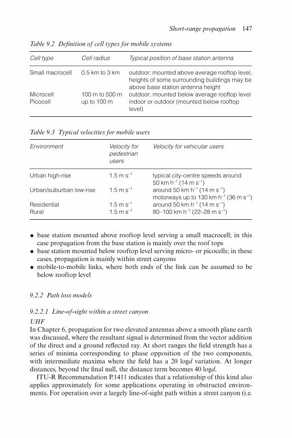
• base station mounted above rooftop level serving a small macrocell; in thiscase propagation from the base station is mainly over the roof tops
• base station mounted below rooftop level serving micro- or picocells; in thesecases, propagation is mainly within street canyons
• mobile-to-mobile links, where both ends of the link can be assumed to bebelow rooftop level
9.2.2 Path loss models
9.2.2.1 Line-of-sight within a street canyon
UHF
In Chapter 6, propagation for two elevated antennas above a smooth plane earthwas discussed, where the resultant signal is determined from the vector additionof the direct and a ground reflected ray. At short ranges the field strength has aseries of minima corresponding to phase opposition of the two components,with intermediate maxima where the field has a 20 logd variation. At longerdistances, beyond the final null, the distance term becomes 40 logd.
ITU-R Recommendation P.1411 indicates that a relationship of this kind alsoapplies approximately for some applications operating in obstructed environ-ments. For operation over a largely line-of-sight path within a street canyon (i.e.
Table 9.2 Definition of cell types for mobile systems
Cell type Cell radius Typical position of base station antenna
Small macrocell 0.5 km to 3 km outdoor; mounted above average rooftop level,heights of some surrounding buildings may beabove base station antenna height
Microcell 100 m to 500 m outdoor; mounted below average rooftop levelPicocell up to 100 m indoor or outdoor (mounted below rooftop
level)
Table 9.3 Typical velocities for mobile users
Environment Velocity forpedestrianusers
Velocity for vehicular users
Urban high-rise 1.5 m s−1 typical city-centre speeds around50 km h−1 (14 m s−1)
Urban/suburban low-rise 1.5 m s−1 around 50 km h−1 (14 m s−1)motorways up to 130 km h−1 (36 m s−1)
Residential 1.5 m s−1 around 50 km h−1 (14 m s−1)Rural 1.5 m s−1 80–100 km h−1 (22–28 m s−1)
Short-range propagation 147
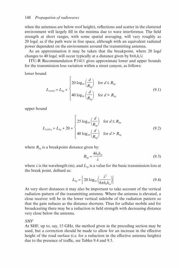
when the antennas are below roof height), reflections and scatter in the clutteredenvironment will largely fill in the minima due to wave interference. The fieldstrength at short ranges, with some spatial averaging, will vary roughly as20 logd, as if the path were in free space, although with an equivalent radiatedpower dependent on the environment around the transmitting antenna.
As an approximation it may be taken that the breakpoint, where 20 logd
changes to 40 logd, will occur typically at a distance given by 8πhthr/λ
ITU-R Recommendation P.1411 gives approximate lower and upper boundsfor the transmission loss variation within a street canyon, as follows:
lower bound
LLOS,l = Lbp +
20 log10 � d
Rbp� for d ≤ Rbp
(9.1)40 log10 � d
Rbp� for d > Rbp
⎧⎪⎨⎪⎩
upper bound
LLOS,u = Lbp + 20 +
25 log10 � d
Rbp� for d ≤ Rbp
(9.2)40 log10 � d
Rbp� for d > Rbp
⎧⎪⎨⎪⎩
where Rbp is a breakpoint distance given by:
Rbp ≈ 4hbhm
λ(9.3)
where λ is the wavelength (m), and Lbp is a value for the basic transmission loss atthe break point, defined as:
Lbp = � 20 log10 � λ2
8πhbhm�� (9.4)
At very short distances it may also be important to take account of the verticalradiation pattern of the transmitting antenna. Where the antenna is elevated, aclose receiver will be in the lower vertical sidelobe of the radiation pattern sothat the gain reduces as the distance shortens. Thus for cellular mobile and forbroadcasting there may be a reduction in field strength with decreasing distancevery close below the antenna.
SHF
At SHF, up to, say, 15 GHz, the method given in the preceding section may beused, but a correction should be made to allow for an increase in the effectiveheight of the road surface (i.e. for a reduction in the effective antenna heights)due to the presence of traffic, see Tables 9.4 and 9.5.
148 Propagation of radiowaves
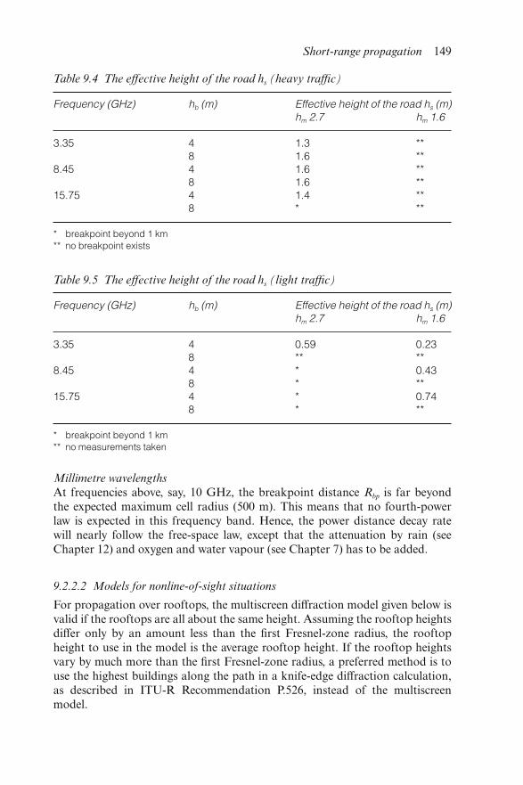
Millimetre wavelengths
At frequencies above, say, 10 GHz, the breakpoint distance Rbp is far beyondthe expected maximum cell radius (500 m). This means that no fourth-powerlaw is expected in this frequency band. Hence, the power distance decay ratewill nearly follow the free-space law, except that the attenuation by rain (seeChapter 12) and oxygen and water vapour (see Chapter 7) has to be added.
9.2.2.2 Models for nonline-of-sight situations
For propagation over rooftops, the multiscreen diffraction model given below isvalid if the rooftops are all about the same height. Assuming the rooftop heightsdiffer only by an amount less than the first Fresnel-zone radius, the rooftopheight to use in the model is the average rooftop height. If the rooftop heightsvary by much more than the first Fresnel-zone radius, a preferred method is touse the highest buildings along the path in a knife-edge diffraction calculation,as described in ITU-R Recommendation P.526, instead of the multiscreenmodel.
Table 9.4 The effective height of the road hs (heavy traffic)
Frequency (GHz) hb (m) Effective height of the road hs (m)hm 2.7 hm 1.6
3.35 4 1.3 **8 1.6 **
8.45 4 1.6 **8 1.6 **
15.75 4 1.4 **8 * **
* breakpoint beyond 1 km** no breakpoint exists
Table 9.5 The effective height of the road hs (light traffic)
Frequency (GHz) hb (m) Effective height of the road hs (m)hm 2.7 hm 1.6
3.35 4 0.59 0.238 ** **
8.45 4 * 0.438 * **
15.75 4 * 0.748 * **
* breakpoint beyond 1 km** no measurements taken
Short-range propagation 149
For rooftops of similar height, the loss between isotropic antennas isexpressed as the sum of free space loss, Lbf, the diffraction loss from rooftop tostreet Lrts and the reduction due to multiple screen diffraction past rows ofbuildings, Lmsd.
In this model Lbf and Lrts are independent of the base station antenna height,and Lmsd is dependent on whether the base station antenna is at, below or abovebuilding heights:
LNLOS1 =Lbf + Lrts + Lmsd for Lrts + Lmsd > 0
(9.5)Lbf for Lrts + Lmsd ≤ 0
⎧⎨⎩
The term Lori describes the coupling of the wave propagating along themultiple-screen path into the street where the mobile station is located. It takesinto account the width of the street and its orientation:
Lrts = −16.9 − 10 log10 (w) + 10 log10 (f) + 20 log10 (Δhm) + Lori (9.6)
−10 + 0.345φ for 0° ≤ φ < 35°
Lori = 2.5 + 0.075 (φ − 35) for 35° ≤ φ < 55° (9.7)
4.0 − 0.114 (φ − 55) for 55° ≤ φ ≤ 90°
⎧⎭⎫⎩
where
Δhm = hr − hm (9.8)
Lori is the street orientation correction factor, which takes into account the effectof rooftop-to-street diffraction into streets that are not perpendicular to thedirection of propagation.
The multiple-screen diffraction loss from the base station due to propagationpast rows of buildings depends on the base station antenna height relative to thebuilding heights and on the incidence angle. A criterion for grazing incidence isthe settled field distance ds:
ds = λd 2
Δhb2
(9.9)
where
Δhb = hb − hr (9.10)
For the calculation of Lmsd, ds is compared with the distance l over which thebuildings extend.
Calculation of Lmsd for l >> ds
Lmsd = Lbsh + ka + kd log10 (d/1000) + kf log10 (f) − 9 log10 (b) (9.11)
where
150 Propagation of radiowaves
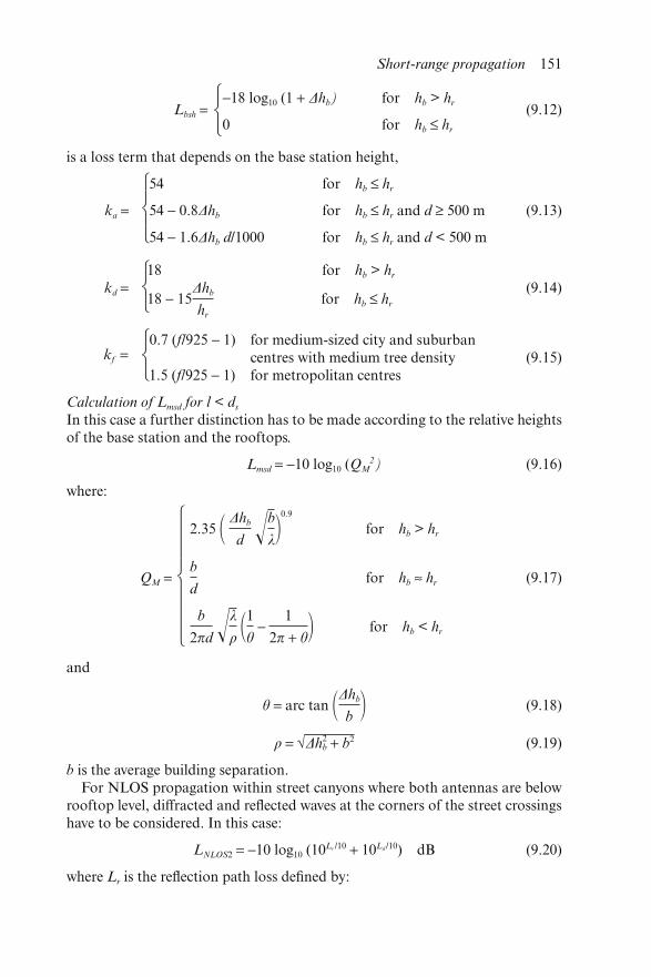
Lbsh =−18 log10 (1 + Δhb) for hb > hr
(9.12)0 for hb ≤ hr
⎧⎨⎩
is a loss term that depends on the base station height,
54 for hb ≤ hr
ka = 54 − 0.8Δhb for hb ≤ hr and d ≥ 500 m (9.13)
54 − 1.6Δhb d/1000 for hb ≤ hr and d < 500 m
⎧⎭⎫⎩
kd = 18 for hb > hr
(9.14)18 − 15
Δhb
hr
for hb ≤ hr
⎧⎨⎩
kf =0.7 (f/925 − 1) for medium-sized city and suburban
centres with medium tree density (9.15)1.5 (f/925 − 1) for metropolitan centres
⎧⎨⎩
Calculation of Lmsd for l < ds
In this case a further distinction has to be made according to the relative heightsof the base station and the rooftops.
Lmsd = −10 log10 (QM2) (9.16)
where:
2.35 � Δhb
d �b
λ�0.9
for hb > hr
QM =b
dfor hb ≈ hr (9.17)
b
2πd �λ
ρ �1θ − 1
2π + θ� for hb < hr
⎧⎪⎪⎭⎫⎪⎪⎩
and
θ = arc tan �Δhb
b � (9.18)
ρ = √Δh2b + b2 (9.19)
b is the average building separation.For NLOS propagation within street canyons where both antennas are below
rooftop level, diffracted and reflected waves at the corners of the street crossingshave to be considered. In this case:
LNLOS2 = −10 log10 (10Lr /10 + 10Ld /10) dB (9.20)
where Lr is the reflection path loss defined by:
Short-range propagation 151
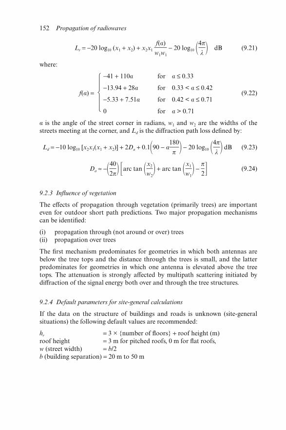
Lr = −20 log10 (x1 + x2) + x2x1 f(α)
w1w1
− 20 log10 �4π
λ � dB (9.21)
where:
−41 + 110α for α ≤ 0.33
f(α) =−13.94 + 28α for 0.33 < α ≤ 0.42
(9.22)−5.33 + 7.51α for 0.42 < α ≤ 0.71
0 for α > 0.71
⎧⎪⎨⎪⎩
α is the angle of the street corner in radians, w1 and w2 are the widths of thestreets meeting at the corner, and Ld is the diffraction path loss defined by:
Ld = −10 log10 [x2x1(x1 + x2)] + 2Da + 0.1�90 − α180
π � − 20 log10 �4π
λ � dB (9.23)
Da ≈ −�40
2π� arc tan �x2
w2� + arc tan �x1
w1� −
π
2� (9.24)
9.2.3 Influence of vegetation
The effects of propagation through vegetation (primarily trees) are importanteven for outdoor short path predictions. Two major propagation mechanismscan be identified:
(i) propagation through (not around or over) trees(ii) propagation over trees
The first mechanism predominates for geometries in which both antennas arebelow the tree tops and the distance through the trees is small, and the latterpredominates for geometries in which one antenna is elevated above the treetops. The attenuation is strongly affected by multipath scattering initiated bydiffraction of the signal energy both over and through the tree structures.
9.2.4 Default parameters for site-general calculations
If the data on the structure of buildings and roads is unknown (site-generalsituations) the following default values are recommended:
hr = 3 × {number of floors} + roof height (m)roof height = 3 m for pitched roofs, 0 m for flat roofs,w (street width) = b/2b (building separation) = 20 m to 50 m
152 Propagation of radiowaves
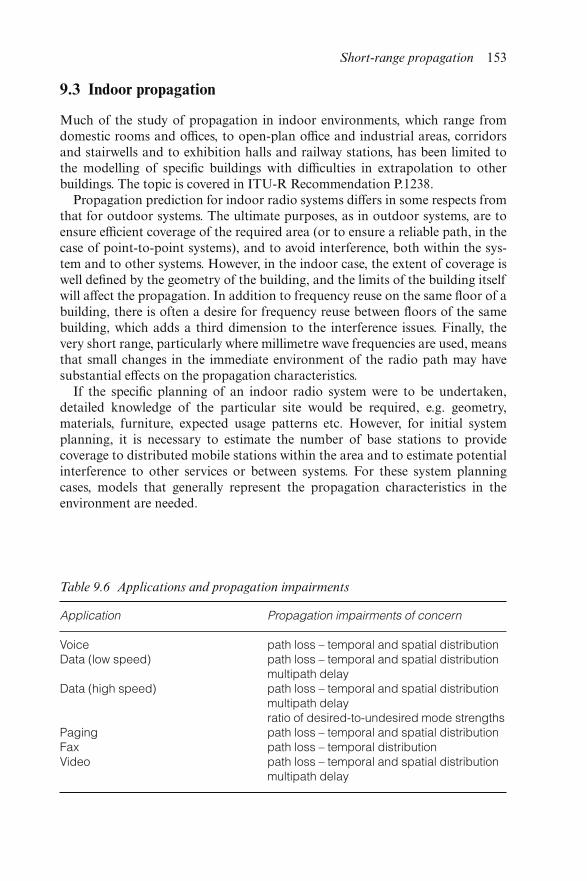
9.3 Indoor propagation
Much of the study of propagation in indoor environments, which range fromdomestic rooms and offices, to open-plan office and industrial areas, corridorsand stairwells and to exhibition halls and railway stations, has been limited tothe modelling of specific buildings with difficulties in extrapolation to otherbuildings. The topic is covered in ITU-R Recommendation P.1238.
Propagation prediction for indoor radio systems differs in some respects fromthat for outdoor systems. The ultimate purposes, as in outdoor systems, are toensure efficient coverage of the required area (or to ensure a reliable path, in thecase of point-to-point systems), and to avoid interference, both within the sys-tem and to other systems. However, in the indoor case, the extent of coverage iswell defined by the geometry of the building, and the limits of the building itselfwill affect the propagation. In addition to frequency reuse on the same floor of abuilding, there is often a desire for frequency reuse between floors of the samebuilding, which adds a third dimension to the interference issues. Finally, thevery short range, particularly where millimetre wave frequencies are used, meansthat small changes in the immediate environment of the radio path may havesubstantial effects on the propagation characteristics.
If the specific planning of an indoor radio system were to be undertaken,detailed knowledge of the particular site would be required, e.g. geometry,materials, furniture, expected usage patterns etc. However, for initial systemplanning, it is necessary to estimate the number of base stations to providecoverage to distributed mobile stations within the area and to estimate potentialinterference to other services or between systems. For these system planningcases, models that generally represent the propagation characteristics in theenvironment are needed.
Table 9.6 Applications and propagation impairments
Application Propagation impairments of concern
Voice path loss – temporal and spatial distributionData (low speed) path loss – temporal and spatial distribution
multipath delayData (high speed) path loss – temporal and spatial distribution
multipath delayratio of desired-to-undesired mode strengths
Paging path loss – temporal and spatial distributionFax path loss – temporal distributionVideo path loss – temporal and spatial distribution
multipath delay
Short-range propagation 153
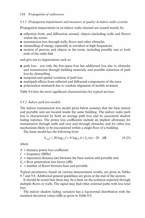
9.3.1 Propagation impairments and measures of quality in indoor radio systems
Propagation impairments in an indoor radio channel are caused mainly by:
• reflection from, and diffraction around, objects (including walls and floors)within the rooms
• transmission loss through walls, floors and other obstacles
• channelling of energy, especially in corridors at high frequencies
• motion of persons and objects in the room, including possibly one or bothends of the radio link
and give rise to impairments such as:
• path loss – not only the free-space loss but additional loss due to obstaclesand transmission through building materials, and possible reduction of pathloss by channelling
• temporal and spatial variation of path loss
• multipath effects from reflected and diffracted components of the wave
• polarisation mismatch due to random alignment of mobile terminal.
Table 9.6 lists the most significant characteristics for typical services.
9.3.2 Indoor path loss models
The indoor transmission loss model given below assumes that the base stationand portable unit are located inside the same building. The indoor radio pathloss is characterised by both an average path loss and its associated shadowfading statistics. The power loss coefficients include an implicit allowance fortransmission through walls and over and through obstacles, and for other lossmechanisms likely to be encountered within a single floor of a building.
The basic model has the following form:
Ltotal = 20 log10 f + N log10 d + Lf (n) − 28 dB (9.25)
where
N = distance power loss coefficientf = frequency (MHz)d = separation distance (m) between the base station and portable unitLf = floor penetration loss factor (dB)n = number of floors between base and portable
Typical parameters, based on various measurement results, are given in Tables9.7 and 9.8. Additional general guidelines are given at the end of the section.
It should be noted that there may be a limit on the isolation expected throughmultiple floors or walls. The signal may find other external paths with less totalloss.
The indoor shadow fading variation has a log-normal distribution with thestandard deviation values (dB) as given in Table 9.9.
154 Propagation of radiowaves
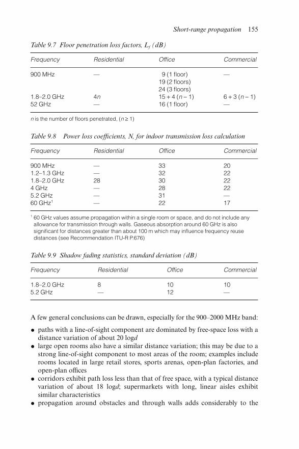
A few general conclusions can be drawn, especially for the 900–2000 MHz band:
• paths with a line-of-sight component are dominated by free-space loss with adistance variation of about 20 logd
• large open rooms also have a similar distance variation; this may be due to astrong line-of-sight component to most areas of the room; examples includerooms located in large retail stores, sports arenas, open-plan factories, andopen-plan offices
• corridors exhibit path loss less than that of free space, with a typical distancevariation of about 18 logd; supermarkets with long, linear aisles exhibitsimilar characteristics
• propagation around obstacles and through walls adds considerably to the
Table 9.7 Floor penetration loss factors, Lf (dB)
Frequency Residential Office Commercial
900 MHz — 9 (1 floor)19 (2 floors)24 (3 floors)
—
1.8–2.0 GHz 4n 15 + 4 (n − 1) 6 + 3 (n − 1)52 GHz — 16 (1 floor) —
n is the number of floors penetrated, (n ≥ 1)
Table 9.8 Power loss coefficients, N, for indoor transmission loss calculation
Frequency Residential Office Commercial
900 MHz — 33 201.2–1.3 GHz — 32 221.8–2.0 GHz 28 30 224 GHz — 28 225.2 GHz — 31 —60 GHz1 — 22 17
1 60 GHz values assume propagation within a single room or space, and do not include anyallowance for transmission through walls. Gaseous absorption around 60 GHz is alsosignificant for distances greater than about 100 m which may influence frequency reusedistances (see Recommendation ITU-R P.676)
Table 9.9 Shadow fading statistics, standard deviation (dB)
Frequency Residential Office Commercial
1.8–2.0 GHz 8 10 105.2 GHz — 12 —
Short-range propagation 155
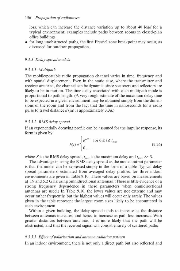
loss, which can increase the distance variation up to about 40 logd for atypical environment; examples include paths between rooms in closed-planoffice buildings
• for long unobstructed paths, the first Fresnel zone breakpoint may occur, asdiscussed for outdoor propagation.
9.3.3 Delay spread models
9.3.3.1 Multipath
The mobile/portable radio propagation channel varies in time, frequency andwith spatial displacement. Even in the static case, where the transmitter andreceiver are fixed, the channel can be dynamic, since scatterers and reflectors arelikely to be in motion. The time delay associated with each multipath mode isproportional to path length. (A very rough estimate of the maximum delay timeto be expected in a given environment may be obtained simply from the dimen-sions of the room and from the fact that the time in nanoseconds for a radiopulse to travel distance d (m) is approximately 3.3d.)
9.3.3.2 RMS delay spread
If an exponentially decaying profile can be assumed for the impulse response, itsform is given by:
h(t) =e−t/S for 0 ≤ t ≤ tmax
(9.26)0 . . .
⎧⎨⎩
where S is the RMS delay spread, tmax is the maximum delay and tmax >> S.The advantage in using the RMS delay spread as the model output parameter
is that the model can be expressed simply in the form of a table. Typical delayspread parameters, estimated from averaged delay profiles, for three indoorenvironments are given in Table 9.10. These values are based on measurementsat 1.9 and 5.2 GHz using omnidirectional antennas. (There is little evidence of astrong frequency dependence in these parameters when omnidirectionalantennas are used.) In Table 9.10, the lower values are not extreme and mayoccur rather frequently, but the highest values will occur only rarely. The valuesgiven in the table represent the largest room sizes likely to be encountered ineach environment.
Within a given building, the delay spread tends to increase as the distancebetween antennas increases, and hence to increase as path loss increases. Withgreater distances between antennas, it is more likely that the path will beobstructed, and that the received signal will consist entirely of scattered paths.
9.3.3.3 Effect of polarisation and antenna radiation pattern
In an indoor environment, there is not only a direct path but also reflected and
156 Propagation of radiowaves
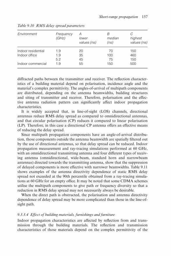
diffracted paths between the transmitter and receiver. The reflection character-istics of a building material depend on polarisation, incidence angle and thematerial’s complex permittivity. The angles-of-arrival of multipath componentsare distributed, depending on the antenna beamwidths, building structuresand siting of transmitter and receiver. Therefore, polarisation and the effec-tive antenna radiation pattern can significantly affect indoor propagationcharacteristics.
It is widely accepted that, in line-of-sight (LOS) channels, directionalantennas reduce RMS delay spread as compared to omnidirectional antennas,and that circular polarisation (CP) reduces it compared to linear polarisation(LP). Therefore, in this case a directional CP antenna offers an effective meansof reducing the delay spread.
Since multipath propagation components have an angle-of-arrival distribu-tion, those components outside the antenna beamwidth are spatially filtered outby the use of directional antennas, so that delay spread can be reduced. Indoorpropagation measurement and ray-tracing simulations performed at 60 GHz,with an omnidirectional transmitting antenna and four different types of receiv-ing antenna (omnidirectional, wide-beam, standard horn and narrowbeamantennas) directed towards the transmitting antenna, show that the suppressionof delayed components is more effective with narrower beamwidths. Table 9.11shows examples of the antenna directivity dependence of static RMS delayspread not exceeded at the 90th percentile obtained from a ray-tracing simula-tions at 60 GHz for an empty office. It may be noted that some CDMA schemesutilise the multipath components to give path or frequency diversity so that areduction in RMS delay spread may not necessarily always be desirable.
When the direct path is obstructed, the polarisation and antenna directivitydependence of delay spread may be more complicated than those in the line-of-sight path.
9.3.3.4 Effect of building materials, furnishings and furniture
Indoor propagation characteristics are affected by reflection from and trans-mission through the building materials. The reflection and transmissioncharacteristics of those materials depend on the complex permittivity of the
Table 9.10 RMS delay spread parameters
Environment Frequency(GHz)
Alowervalues (ns)
Bmedian(ns)
Chighestvalues (ns)
Indoor residential 1.9 20 70 150Indoor office 1.9
5.23545
10075
460150
Indoor commercial 1.9 55 150 500
Short-range propagation 157
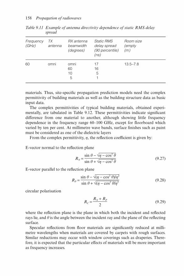
materials. Thus, site-specific propagation prediction models need the complexpermittivity of building materials as well as the building structure data as basicinput data.
The complex permittivities of typical building materials, obtained experi-mentally, are tabulated in Table 9.12. These permittivities indicate significantdifference from one material to another, although showing little frequencydependence in the frequency range 60–100 GHz, except for floorboard whichvaried by ten per cent. At millimetre wave bands, surface finishes such as paintmust be considered as one of the dielectric layers
From the complex permittivity, η, the reflection coefficient is given by:
E-vector normal to the reflection plane
RN = sin θ − √η − cos2 θ
sin θ + √η − cos2 θ(9.27)
E-vector parallel to the reflection plane
RP = sin θ − √(η − cos2 θ)/η2
sin θ + √(η − cos2 θ/η2(9.28)
circular polarisation
RC = RN + RP
2(9.29)
where the reflection plane is the plane in which both the incident and reflectedrays lie, and θ is the angle between the incident ray and the plane of the reflectingsurface.
Specular reflections from floor materials are significantly reduced at milli-metre wavelengths when materials are covered by carpets with rough surfaces.Similar reductions may occur with window coverings such as draperies. There-fore, it is expected that the particular effects of materials will be more importantas frequency increases.
Table 9.11 Example of antenna directivity dependence of static RMS delayspread
Frequency(GHz)
TXantenna
RX antennabeamwidth(degrees)
Static RMSdelay spread(90 percentile)(ns)
Room size(empty(m)
60 omni omni60105
171651
13.5∼7.8
158 Propagation of radiowaves
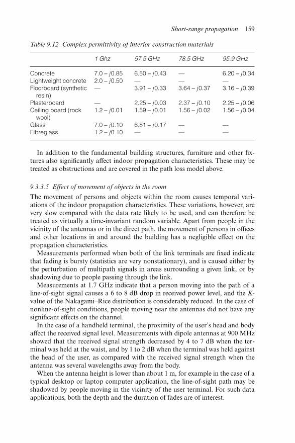
In addition to the fundamental building structures, furniture and other fix-tures also significantly affect indoor propagation characteristics. These may betreated as obstructions and are covered in the path loss model above.
9.3.3.5 Effect of movement of objects in the room
The movement of persons and objects within the room causes temporal vari-ations of the indoor propagation characteristics. These variations, however, arevery slow compared with the data rate likely to be used, and can therefore betreated as virtually a time-invariant random variable. Apart from people in thevicinity of the antennas or in the direct path, the movement of persons in officesand other locations in and around the building has a negligible effect on thepropagation characteristics.
Measurements performed when both of the link terminals are fixed indicatethat fading is bursty (statistics are very nonstationary), and is caused either bythe perturbation of multipath signals in areas surrounding a given link, or byshadowing due to people passing through the link.
Measurements at 1.7 GHz indicate that a person moving into the path of aline-of-sight signal causes a 6 to 8 dB drop in received power level, and the K-value of the Nakagami–Rice distribution is considerably reduced. In the case ofnonline-of-sight conditions, people moving near the antennas did not have anysignificant effects on the channel.
In the case of a handheld terminal, the proximity of the user’s head and bodyaffect the received signal level. Measurements with dipole antennas at 900 MHzshowed that the received signal strength decreased by 4 to 7 dB when the ter-minal was held at the waist, and by 1 to 2 dB when the terminal was held againstthe head of the user, as compared with the received signal strength when theantenna was several wavelengths away from the body.
When the antenna height is lower than about 1 m, for example in the case of atypical desktop or laptop computer application, the line-of-sight path may beshadowed by people moving in the vicinity of the user terminal. For such dataapplications, both the depth and the duration of fades are of interest.
Table 9.12 Complex permittivity of interior construction materials
1 Ghz 57.5 GHz 78.5 GHz 95.9 GHz
Concrete 7.0 − j0.85 6.50 − j0.43 — 6.20 − j0.34Lightweight concrete 2.0 − j0.50 — — —Floorboard (synthetic
resin)— 3.91 − j0.33 3.64 − j0.37 3.16 − j0.39
Plasterboard — 2.25 − j0.03 2.37 − j0.10 2.25 − j0.06Ceiling board (rock
wool)1.2 − j0.01 1.59 − j0.01 1.56 − j0.02 1.56 − j0.04
Glass 7.0 − j0.10 6.81 − j0.17 — —Fibreglass 1.2 − j0.10 — — —
Short-range propagation 159
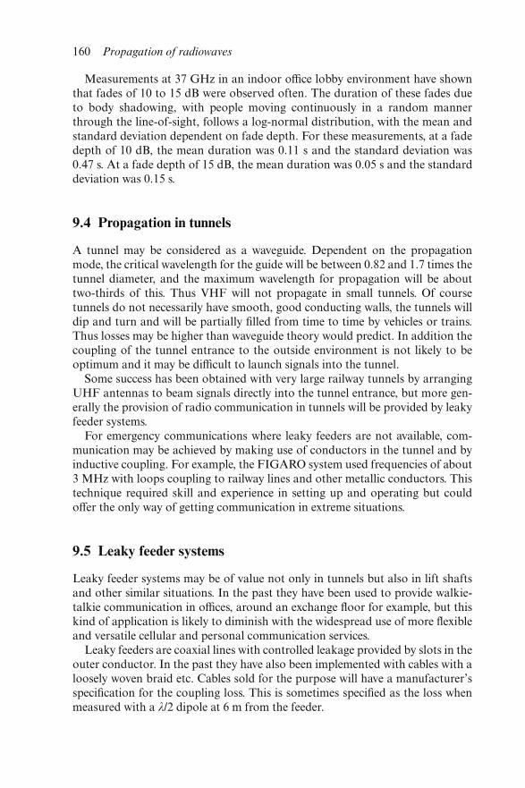
Measurements at 37 GHz in an indoor office lobby environment have shownthat fades of 10 to 15 dB were observed often. The duration of these fades dueto body shadowing, with people moving continuously in a random mannerthrough the line-of-sight, follows a log-normal distribution, with the mean andstandard deviation dependent on fade depth. For these measurements, at a fadedepth of 10 dB, the mean duration was 0.11 s and the standard deviation was0.47 s. At a fade depth of 15 dB, the mean duration was 0.05 s and the standarddeviation was 0.15 s.
9.4 Propagation in tunnels
A tunnel may be considered as a waveguide. Dependent on the propagationmode, the critical wavelength for the guide will be between 0.82 and 1.7 times thetunnel diameter, and the maximum wavelength for propagation will be abouttwo-thirds of this. Thus VHF will not propagate in small tunnels. Of coursetunnels do not necessarily have smooth, good conducting walls, the tunnels willdip and turn and will be partially filled from time to time by vehicles or trains.Thus losses may be higher than waveguide theory would predict. In addition thecoupling of the tunnel entrance to the outside environment is not likely to beoptimum and it may be difficult to launch signals into the tunnel.
Some success has been obtained with very large railway tunnels by arrangingUHF antennas to beam signals directly into the tunnel entrance, but more gen-erally the provision of radio communication in tunnels will be provided by leakyfeeder systems.
For emergency communications where leaky feeders are not available, com-munication may be achieved by making use of conductors in the tunnel and byinductive coupling. For example, the FIGARO system used frequencies of about3 MHz with loops coupling to railway lines and other metallic conductors. Thistechnique required skill and experience in setting up and operating but couldoffer the only way of getting communication in extreme situations.
9.5 Leaky feeder systems
Leaky feeder systems may be of value not only in tunnels but also in lift shaftsand other similar situations. In the past they have been used to provide walkie-talkie communication in offices, around an exchange floor for example, but thiskind of application is likely to diminish with the widespread use of more flexibleand versatile cellular and personal communication services.
Leaky feeders are coaxial lines with controlled leakage provided by slots in theouter conductor. In the past they have also been implemented with cables with aloosely woven braid etc. Cables sold for the purpose will have a manufacturer’sspecification for the coupling loss. This is sometimes specified as the loss whenmeasured with a λ/2 dipole at 6 m from the feeder.
160 Propagation of radiowaves
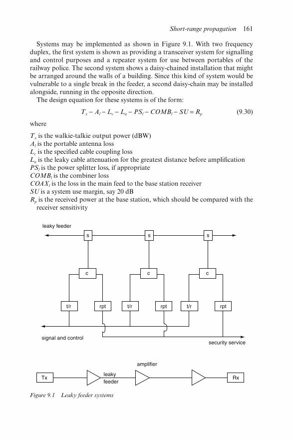
Systems may be implemented as shown in Figure 9.1. With two frequencyduplex, the first system is shown as providing a transceiver system for signallingand control purposes and a repeater system for use between portables of therailway police. The second system shows a daisy-chained installation that mightbe arranged around the walls of a building. Since this kind of system would bevulnerable to a single break in the feeder, a second daisy-chain may be installedalongside, running in the opposite direction.
The design equation for these systems is of the form:
Tx − Al − Lc − La − PSl − COMBl − SU = Rp (9.30)
where
Tx is the walkie-talkie output power (dBW)Al is the portable antenna lossLc is the specified cable coupling lossLa is the leaky cable attenuation for the greatest distance before amplificationPSl is the power splitter loss, if appropriateCOMBl is the combiner lossCOAXl is the loss in the main feed to the base station receiverSU is a system use margin, say 20 dBRp is the received power at the base station, which should be compared with the
receiver sensitivity
Figure 9.1 Leaky feeder systems
Short-range propagation 161
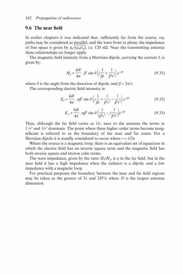
9.6 The near field
In earlier chapters it was indicated that, sufficiently far from the source, raypaths may be considered as parallel, and the wave front as plane; the impedanceof free space is given by η0√(μ0/ε0), i.e. 120 πΩ. Near the transmitting antennathese relationships no longer apply.
The magnetic field intensity from a Hertzian dipole, carrying the current I, isgiven by:
H = Id�
4π. β2 sin θ �j 1
βr +
1
β2r2� e−jβr (9.31)
where θ is the angle from the direction of dipole, and β = 2π/λ.The corresponding electric field intensity is:
Eθ = Id�
4π. ηβ2 sin θ �j 1
βr +
1
β2r2 −
1
β3r3� e−jβr (9.32)
Eri = Id�
4π. ηβ2 sin θ � 1
β2r2 − j
1
β3r3�e−jβr (9.33)
Thus, although the far field varies as 1/r, near to the antenna the terms in1 /r2 and 1/r3 dominate. The point where these higher order terms become insig-nificant is referred to as the boundary of the near and far zones. For aHertzian dipole it is usually considered to occur where r = λ/2π
Where the source is a magnetic loop, there is an equivalent set of equations inwhich the electric field has an inverse square term and the magnetic field hasboth inverse square and inverse cube terms.
The wave impedance, given by the ratio Hθ/H, is η in the far field, but in thenear field it has a high impedance when the radiator is a dipole, and a lowimpedance with a magnetic loop
For practical purposes the boundary between the near and far field regionsmay be taken as the greater of 3λ and 2D2/λ where D is the largest antennadimension.
162 Propagation of radiowaves
Chapter 10
Numerically intensive propagationprediction methods
C.C. Constantinou
10.1 Introduction
This Chapter aims to introduce a number of deterministic radiowave propaga-tion prediction methods and discuss briefly the computational issues arising intheir practical implementation.
Ideally, we wish to solve Maxwell’s equations exactly by specifying a boun-dary value problem to a sufficient degree of accuracy, subject to some initialconditions. The boundary value problem in this case is the geometrical andelectrical description of the radio environment down to subwavelength accuracy,whereas the initial conditions are the current distribution on the transmittingantenna.
10.1.1 Intractability of exact solutions
Let us consider the numerical complexity in attempting to solve the reducedvector wave equation, which can be derived from Maxwell’s equations. Take atypical GSM900 macrocell of a 10 km radius. A stable numerical solutionrequires that we discretise the domain (macrocell) into a cubic grid whose sizeis at most λ/2 long. Taking the cell height to be 100 m so as to include thetallest possible buildings in it, the minimum required number of grid points is∼πr2h/(λ/2)3 ∼ 7 × 10¹². In the calculation, at each grid point we need to use onecomplex double precision variable for each Cartesian component of the electricfield and one complex double precision variable for the complex dielectric con-stant of the medium. Since a complex double precision variable corresponds to16 bytes of memory, the total amount of memory space required for a straight-forward numerical solution to the problem is ∼ 4 × 1014 bytes, or 400 Tbytes.
A similar consideration applied to the boundary data (i.e. the amount of
information to be extracted from a building and terrain database) shows that thesmallest database that can be used would have a size of at least 100 Gbytes.
Clearly, the problem of solving the full, vector wave equation exactly formeaningful problems in radiowave propagation is intractable for two reasons:
(i) the computational complexity of the problem is beyond the capability ofany computer in the foreseeable future (even taking into account Moore’slaw);
(ii) the collection of the input data at this level of accuracy – even ifautomated fully – is a near practical impossibility.
10.1.2 General remarks on numerical methods
Numerically intensive radiowave propagation prediction methods share onecommon feature: they make judicious use of approximations and simplificationsto render the problem at hand tractable. These approximations may be based onhigh-frequency asymptotic solutions to exact problems, a priori knowledge onthe propagation direction, the paraxial approximation etc. Therefore, no singlepractical solution of Maxwell’s equations exists that is applicable to allpropagation problems.
10.1.3 Chapter outline
In this Chapter, we shall restrict our attention to tropospheric, clear air propaga-tion in the VHF and UHF bands (30 MHz–3 GHz) only. Typical applicationsthat would employ these numerically intensive methods include broadcasting,radar operation prediction and point-to-point radio link and mobile radioplanning.
The deterministic propagation techniques considered here are:
(a) integral equations(b) the parabolic equation(c) ray tracing
In all of the above methods, the dominant consideration will be the terraineffects, whereas in the case of the parabolic equation method the effect of theatmosphere will also be included.
10.2 Integral equation methods
Here we shall consider only one integral equation formulation, based onHufford’s original work [1]. This formulation is based on the use of Green’sintegral theorem and approximate boundary conditions. For simplicity we shallconsider only the case of an elevated Hertzian dipole source over an irregular,inhomogeneous earth.
164 Propagation of radiowaves
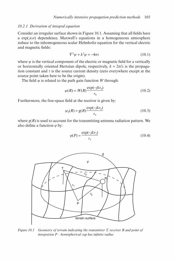
10.2.1 Derivation of integral equation
Consider an irregular surface shown in Figure 10.1. Assuming that all fields havea exp( jωt) dependence, Maxwell’s equations in a homogeneous atmospherereduce to the inhomogeneous scalar Helmholtz equation for the vertical electricand magnetic fields:
∇ 2ψ + k2ψ = −4πτ (10.1)
where ψ is the vertical component of the electric or magnetic field for a verticallyor horizontally oriented Hertzian dipole, respectively, k = 2π/λ is the propaga-tion constant and τ is the source current density (zero everywhere except at thesource point taken here to be the origin).
The field ψ is related to the path gain function W through:
ψ(R) = W(R)exp(−jkr0)
r0
(10.2)
Furthermore, the free-space field at the receiver is given by:
ψ0(R) = g(R)exp(−jkr0)
r0
(10.3)
where g(R) is used to account for the transmitting antenna radiation pattern. Wealso define a function φ by:
φ(P) = exp(−jkr2)
r2
(10.4)
Figure 10.1 Geometry of terrain indicating the transmitter T, receiver R and point of
integration P – hemispherical cap has infinite radius
Numerically intensive propagation prediction methods 165
related to the free-space Green’s function and satisfying the homogeneous scalarHelmholtz equation:
∇ 2φ + k2φ = 0 (10.5)
Finally, the field ψ satisfies the simple Leontovich [2] boundary condition:
∂ψ
∂n(P) = jkδψ(P) (10.6a)
where
δ = �√ε − 1/ε for vertical polarisation (10.6b)
√ε − 1 for horizontal polarisation
and ε = εr + jσ/ωε0 is the complex dielectric constant for the ground.Green’s theorem states that any two continuous differentiable scalar functions
of position ψ and φ defined in a closed volume V bounded by a surface S = ∂V
satisfy:
��v
�(ψ∇ 2φ − φ∇ 2ψ)dV = �s
�φ∂ψ
∂n −ψ
∂φ
∂n�da (10.7)
where ∂/∂n denotes a normal derivative. We define the volume V to be that of thehemisphere shown in Figure 10.1 minus the volume of an infinitesimally smallsphere surrounding the receiving point. Using Eqns. 10.1, 10.4, 10.5 and 10.6Green’s theorem reduces to:
��v
�(ψ(−k2φ) − φ(−k2ψ − 4πτ))dV
= �s
�exp(−jkr2)
r2
⋅ jkδψ − ψ ⋅ exp(− jkr2)
r2
jk�−1 −1
jkr2�∂r2
∂n�da + 4πψ(R) (10.8)
where the last term arises from the surface integral around the infinitesimallysmall sphere centred at the receiving point. The left-hand side of Eqn. 10.8identically simplifies to 4πψ0(R). Finally, using Eqns. 10.2 and 10.3 to derive anequation for the path gain function and after some rearranging Eqn. 10.8 can bereduced to:
W(R) = g(R)−jk
4π ��W(P)exp(− jk[r1 + r2 − r0])
r0
r1r2�δ + �1 +
1
jkr2�∂r2
∂n�da (10.9)
earth’ssurface
where we have made use of the fact that as the radius of the hemisphere tends toinfinity, the radiation condition ensures that we have no contribution to theintegral from the hemispherical cap.
166 Propagation of radiowaves
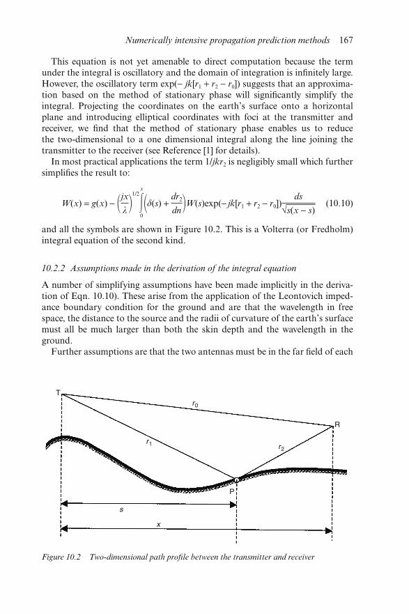
This equation is not yet amenable to direct computation because the termunder the integral is oscillatory and the domain of integration is infinitely large.However, the oscillatory term exp(− jk[r1 + r2 − r0]) suggests that an approxima-tion based on the method of stationary phase will significantly simplify theintegral. Projecting the coordinates on the earth’s surface onto a horizontalplane and introducing elliptical coordinates with foci at the transmitter andreceiver, we find that the method of stationary phase enables us to reducethe two-dimensional to a one dimensional integral along the line joining thetransmitter to the receiver (see Reference [1] for details).
In most practical applications the term 1/jkr2 is negligibly small which furthersimplifies the result to:
W(x) = g(x) − �jxλ �1/2
�x
0
�δ(s) + dr2
dn�W(s)exp(− jk[r1 + r2 − r0])ds
√s(x − s)(10.10)
and all the symbols are shown in Figure 10.2. This is a Volterra (or Fredholm)integral equation of the second kind.
10.2.2 Assumptions made in the derivation of the integral equation
A number of simplifying assumptions have been made implicitly in the deriva-tion of Eqn. 10.10). These arise from the application of the Leontovich imped-ance boundary condition for the ground and are that the wavelength in freespace, the distance to the source and the radii of curvature of the earth’s surfacemust all be much larger than both the skin depth and the wavelength in theground.
Further assumptions are that the two antennas must be in the far field of each
Figure 10.2 Two-dimensional path profile between the transmitter and receiver
Numerically intensive propagation prediction methods 167
other and that the transverse terrain variation to the path profile between thetransmitter and the receiver (great circle path) is sufficiently slow in order not toinvalidate the stationary phase analysis results. This latter approximation breaksdown when there are strong reflected field components from laterally displacedterrain obstacles, as is often the case. Thus, the main approximation arises ingoing from Eqn. 10.9 to Eqn. 10.10.
10.2.3 Numerical evaluation of integral equations
The integral Eqn. 10.10 can only be easily solved at low to medium frequencieswhen the oscillating exponential exp(− jk [r1 + r2 − r0]) does not vary too rapidly.At high frequencies (typically in the UHF band and above) the numerical evalu-ation of the integral equation tends to become unstable resulting in significantloss of accuracy.
To evaluate Eqn. 10.10 we start by first solving the corresponding equation fora ground-based receiver. This is done by discretising the domain of integrationinto subintervals and solving this in an iterative manner as follows.
Dividing the interval [0, x] into m steps each of length h then yields:
W(nh) = g(mh) − �jmh
λ �1/2
×
�m−1
i=0�h
0
W(ih + y)�δ(ih + y) + dr2
dn�exp(− jk[r1 + r2 − r0])dy
√(ih + y)(mh − ih − y)(10.11)
Any discrete approximation to the integral in Eqn. 10.11 will contain only oneW(mh) term, which can then be moved to the left-hand side of the equation.Therefore, the integral equation becomes an iterative equation as the mth termonly depends on the previous m − 1 terms. Care needs to be taken in the numer-ical integration scheme at the two endpoints as they both have an integrable
singularity of the form �h
0
dx/√x = 2√h.
Furthermore, the method usually requires the a priori knowledge of at leastthe first, if not the first few, terms in the sequence {W(0), W(h), W(2h), . . . }.Estimating these first few values accurately usually relies on an appropriateanalytical solution such as Sommerfeld’s solution for a plane homogeneousearth, the two-ray model etc.
Finally, at high frequencies identification of the stationary points of the inte-grand in Eqn. 10.10 as a function of x can be exploited to assist the accuratenumerical evaluation of the iterative Eqn. 10.11.
When the path gain function is found for all points on the ground along thepath between the transmitter and receiver, deriving the attenuation at an ele-vated receiver is trivial, as we no longer identify the two W(mh) terms on bothsides of Eqn. 10.11. Then using values for r0 and r2 appropriate to the elevatedantenna we evaluate this equation one last time.
168 Propagation of radiowaves
As software capable of performing computations of (similar) integral equa-tions is readily available [3], no numerical result examples will be presented here.
10.3 Parabolic equation methods
The parabolic equation is an example of a full-wave method, which attempts todirectly solve the wave equation numerically, subject to a number of assump-tions and simplifications. The method was derived as far back as the 1940s byLeontovich and Fock [4], but was deemed too computationally intensive tobecome a practical prediction tool.
With the advent of digital computers it found widespread use in underwateracoustic propagation prediction in the 1970s and 1980s [5, 6]. In underwateracoustics the wavelength tends to be long, thus easing the computationalrequirements somewhat.
By the 1990s, digital computers became fast enough and the parabolic equa-tion method was applied to model propagation of radiowaves up to the UHFand SHF frequencies in the troposphere [7–9].
10.3.1 Derivation of the parabolic equation
Once again, we begin by reducing Maxwell’s equations to the Helmholtz equa-tion. However, in this instance we assume the presence of an atmospheredescribed by a complex refractive index:
n(r) = √ε(r) = √εr(r) + jσ(r)ωε0 (10.12)
which is a continuously varying function of position. Provided that λ0∇ ln n<<1,the scalar Helmholtz equation describes accurately each of the Cartesiancomponents of the electric and magnetic fields,
∇ 2ψ + k20n
2ψ = 0 (10.13)
The wavenumber in vacuo is now given by k0 = 2π/λ0. Considering a two-dimensional propagation problem along the great circle path and making theapproximation that the earth is flat1 for simplicity, Eqn. 10.13 can be expandedin Cartesian co-ordinates as:
∂2ψ
∂x2 +
∂2ψ
∂z2 + k2
0n2ψ = 0 (10.14)
We now introduce the assumption that an a priori preferred direction of propa-gation exists and identify this with the x axis. It is, therefore, reasonable that wecan write the following form for the solution:
1 The derivation of the parabolic equation in spherical co-ordinates appropriate to a spherical earthand the subsequent transformation to a (range, height) rectangular co-ordinate system is covered inReference [7] and only changes the term (n2 − 1) in Eqn. 10.16 through to Eqn. 10.23 to (n2 − 1 − 2z/ae)where ae is the effective earth radius
Numerically intensive propagation prediction methods 169
ψ(x,z) = u(x,z)exp(− jk0x) (10.15)
where the reduced wave amplitude u(x,z) can now be assumed to vary slowlyalong the x direction on the scale of a free-space wavelength, λ. SubstitutingEqn. 10.15 into Eqn. 10.14 and discarding the common factor exp(− jk0x) afterperforming the differentiations, yields the following equation for the reducedwave amplitude:
∂2u
∂x2 −2jk0
∂u
∂x +
∂2u
∂z2 + k2
0(n2 − 1)u = 0 (10.16)
Eqn. 10.16 describes waves propagating both along the positive and negativex directions. By analogy with the one-dimensional wave equation
∂2w
∂x2 −
1
c2
∂2w
∂t2 = 0 ⇒ � ∂
∂x −
1
c
∂∂t��
∂∂x
+ 1
c
∂∂t�w = 0 (10.17a)
which has linearly independent solutions
w = ƒ(x − ct) and w = g(x + ct) (10.17b)
which can be identified as forward and backward travelling waves correspondingto the two differential operators in Eqn. 10.17a. We factorise Eqn. 10.16 intoforward and backward travelling wave operators:
� ∂∂x
− jk0 + jk0 �1 + (n2 − 1) + 1
k20
∂∂z2 �×
� ∂∂x
− jk0 − jk0 �1 + (n2 − 1) + 1
k20
∂2
∂z2 �u = 0 (10.18)
and discard the backward travelling wave for consistency with Eqn. 10.15, whichfinally gives:
� ∂∂x
− jk0 + jk0 �1 + (n2 − 1) + 1
k20
∂2
∂z2 �u = 0 (10.19)
It is to be understood that the differential operator under the square root sign inEqn. 10.19 can only be interpreted in a formal sense. Its numerical evaluationcan only be achieved by replacing the square root by a power series, or rationalfractions, of operators, as we shall shortly see.
Thus, we rewrite Eqn. 10.19 as:
∂u
∂x = jk0�1 − �1 + (n2 − 1) +
1
k20
∂2
∂z2 �u ≡ jk0�1 − √1 + Q(x,z) �u (10.20)
The differential operator Q(x,z) must give a significantly smaller answer than theunity operator when operated on u(x,z) since, by assumption, the oscillatoryvariation of i(x,z) is predominantly along the x direction, perpendicular to thez axis. Therefore, the z derivative on a scale of a wavelength (1/k0) is much
170 Propagation of radiowaves
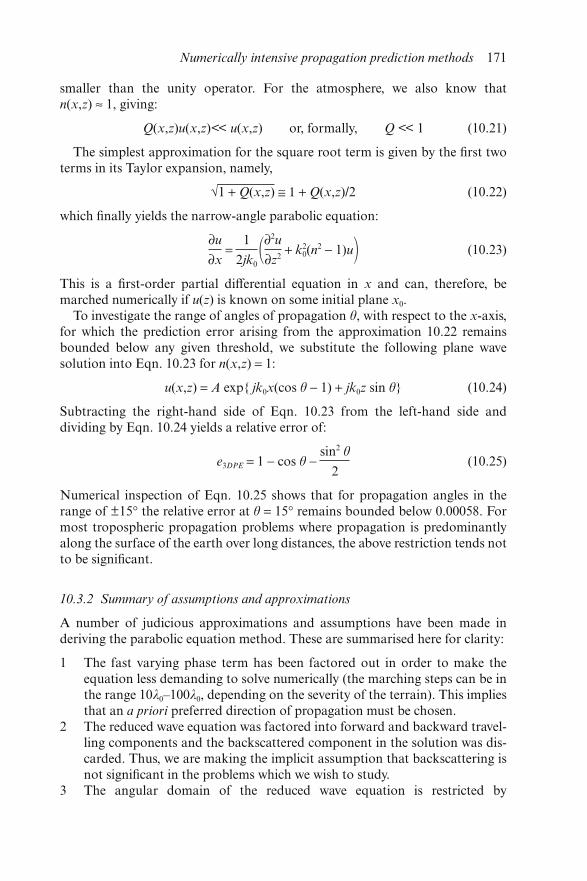
smaller than the unity operator. For the atmosphere, we also know thatn(x,z) ≈ 1, giving:
Q(x,z)u(x,z)<< u(x,z) or, formally, Q << 1 (10.21)
The simplest approximation for the square root term is given by the first twoterms in its Taylor expansion, namely,
√1 + Q(x,z) ≅ 1 + Q(x,z)/2 (10.22)
which finally yields the narrow-angle parabolic equation:
∂u
∂x =
1
2jk0�∂
2u
∂z2 + k0
2(n2 − 1)u� (10.23)
This is a first-order partial differential equation in x and can, therefore, bemarched numerically if u(z) is known on some initial plane x0.
To investigate the range of angles of propagation θ, with respect to the x-axis,for which the prediction error arising from the approximation 10.22 remainsbounded below any given threshold, we substitute the following plane wavesolution into Eqn. 10.23 for n(x,z) = 1:
u(x,z) = A exp{ jk0x(cos θ − 1) + jk0z sin θ} (10.24)
Subtracting the right-hand side of Eqn. 10.23 from the left-hand side anddividing by Eqn. 10.24 yields a relative error of:
e3DPE = 1 − cos θ − sin2 θ
2(10.25)
Numerical inspection of Eqn. 10.25 shows that for propagation angles in therange of ±15° the relative error at θ = 15° remains bounded below 0.00058. Formost tropospheric propagation problems where propagation is predominantlyalong the surface of the earth over long distances, the above restriction tends notto be significant.
10.3.2 Summary of assumptions and approximations
A number of judicious approximations and assumptions have been made inderiving the parabolic equation method. These are summarised here for clarity:
1 The fast varying phase term has been factored out in order to make theequation less demanding to solve numerically (the marching steps can be inthe range 10λ0–100λ0, depending on the severity of the terrain). This impliesthat an a priori preferred direction of propagation must be chosen.
2 The reduced wave equation was factored into forward and backward travel-ling components and the backscattered component in the solution was dis-carded. Thus, we are making the implicit assumption that backscattering isnot significant in the problems which we wish to study.
3 The angular domain of the reduced wave equation is restricted by
Numerically intensive propagation prediction methods 171
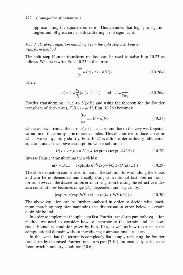
approximating the square root term. This assumes that high propagationangles and off great circle path scattering is not significant.
10.3.3 Parabolic equation marching (I) – the split step fast Fourier
transform method
The split step Fourier transform method can be used to solve Eqn 10.23 asfollows. We first rewrite Eqn. 10.23 in the form:
∂u
∂x = (a(x,z) + bD2
z)u (10.26a)
where
a(x,z) ≡ k0
2j(n2(x,z) − 1) and b ≡
1
2jk0
(10.26b)
Fourier transforming u(x,z) to U (x,kz) and using the theorem for the Fouriertransform of derivatives, F(Dzu) = jkzU, Eqn. 10.26a becomes:
∂U
∂x ≅ aU − k2
z bU (10.27)
where we have treated the term a(x,z) as a constant due to the very weak spatialvariation of the atmospheric refractive index. This of course introduces an errorwhich we will quantify shortly. Eqn. 10.27 is a first-order ordinary differentialequation under the above assumption, whose solution is:
U(x + Δx,kz) = U(x,kz)exp(aΔx)exp(− bk2z Δx) (10.28)
Inverse Fourier transforming then yields:
u(x + Δx,z) = exp(aΔx)F−1(exp(−bk2z Δx)F(u(x,z))) (10.29)
The above equation can be used to march the solution forward along the x axisand can be implemented numerically using conventional fast Fourier trans-forms. However, the discretisation error arising from treating the refractive indexas a constant now becomes range (Δx) dependent and is given by:
{exp(aΔx)exp(bD2z Δx) − exp((a + bD2
z )Δx)}u (10.30)
The above equation can be further analysed in order to decide what maxi-mum marching step size maintains the discretisation error below a certaindesirable bound.
In order to implement the split step fast Fourier transform parabolic equationmethod we need to consider how to incorporate the terrain and its asso-ciated boundary condition given by Eqn. 10.6, as well as how to truncate thecomputational domain without introducing computational artefacts.
In the event that the terrain is completely flat, simply replacing the Fouriertransform by the mixed Fourier transform pair [7,10], automatically satisfies theLeontovich boundary condition (10.6):
172 Propagation of radiowaves
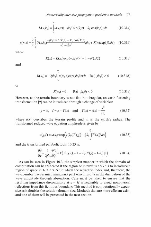
U(x,kz) = �∞
0
u(x,z){− jk0δ sin(kzz) − k2 cos(kzz)}dz (10.31a)
u(x,z) = 2
π �∞
0
U(x,kz)− jk0δ sin(kzz) − kz cos(kzz)
k2z −k2
0δ2
dkz + K(x)exp( jk0δz) (10.31b)
where
K(x) = K(x0)exp{− jk0δ(n2 − 1 − δ2)x/2} (10.31c)
and
K(x0) = −2jk0δ�∞
0
u(x0,z)exp( jk0δz)dz Re(− jk0δ) > 0 (10.31d )
or
K(x0) = 0 Re(− jk0δ) < 0 (10.31e)
However, as the terrain boundary is not flat, but irregular, an earth flatteningtransformation [9] can be introduced through a change of variables:
χ = x, ζ = z − T(x) and T(x) = t(x) − x2
2ae
(10.32)
where t(x) describes the terrain profile and ae is the earth’s radius. Thetransformed reduced wave equation amplitude is given by:
û(χ,ζ) = u(x,z)exp�j [k0ζT′(χ)] + –³²k0�
χ
0
[T′(α)]2dα� (10.33)
and the transformed parabolic Eqn. 10.23 is:
∂û
∂χ =
1
2jk0�∂
2û
∂ζ2 + k2
0[n2(χ,ζ) − 1 − 2ζ{t″(χ) − 1/ae}]û� (10.34)
As can be seen in Figure 10.3, the simplest manner in which the domain ofcomputation can be truncated if the region of interest is z ≤ H is to introduce aregion of space at H ≤ z ≤ 2H in which the refractive index and, therefore, thewavenumber have a small imaginary part which results in the dissipation of thewave amplitude through absorption. Care must be taken to ensure that theresulting impedance discontinuity at z = H is negligible to avoid nonphysicalreflections from this fictitious boundary. This method is computationally expen-sive as it doubles the solution domain size. Methods that are more efficient exist,and one of them will be presented in the next section.
Numerically intensive propagation prediction methods 173
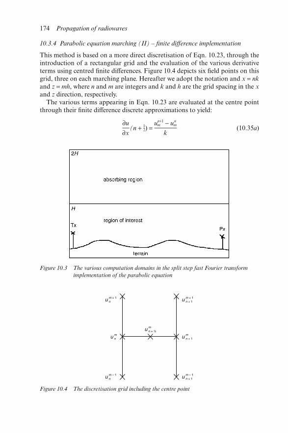
10.3.4 Parabolic equation marching (II) – finite difference implementation
This method is based on a more direct discretisation of Eqn. 10.23, through theintroduction of a rectangular grid and the evaluation of the various derivativeterms using centred finite differences. Figure 10.4 depicts six field points on thisgrid, three on each marching plane. Hereafter we adopt the notation and x = nk
and z = mh, where n and m are integers and k and h are the grid spacing in the xand z direction, respectively.
The various terms appearing in Eqn. 10.23 are evaluated at the centre pointthrough their finite difference discrete approximations to yield:
∂u
∂x(n + 12) =
un+1m − un
m
k(10.35a)
Figure 10.3 The various computation domains in the split step fast Fourier transform
implementation of the parabolic equation
Figure 10.4 The discretisation grid including the centre point
174 Propagation of radiowaves
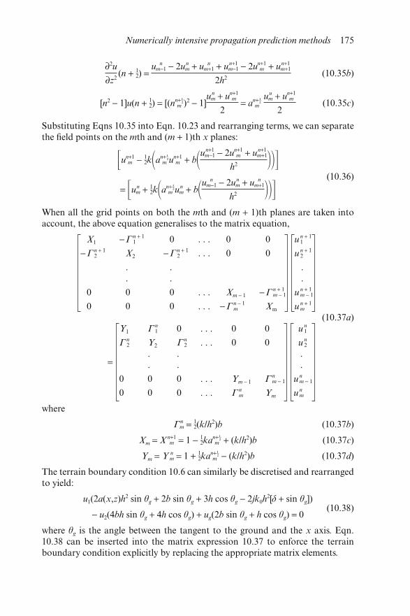
∂2u
∂z2(n + 12) =
u nm−1 − 2un
m + u nm+1 + un+1
m−1 − 2un+1m + un+1
m+1
2h2(10.35b)
[n2 − 1]u(n + 12) = [(nn+–¹²m )2 − 1]
unm + un+1
m
2 = an+–¹
²m uu
m + un+1m
2(10.35c)
Substituting Eqns 10.35 into Eqn. 10.23 and rearranging terms, we can separatethe field points on the mth and (m + 1)th x planes:
un+1m − 12k�an+–¹
²m un+1m + b�u
n+1m−1 − 2un+1
m + un+1m+1
h2 ���
= unm + 12k�an+–¹
²m unm + b�u
nm−1 − 2un
m + u nm+1
h2 ���(10.36)
When all the grid points on both the mth and (m + 1)th planes are taken intoaccount, the above equation generalises to the matrix equation,
X1 −Γ n + 11 0 . . . 0 0 u n + 1
1
−Γ n + 12 X2 −Γ n + 1
2 . . . 0 0 u n + 12
. . .
. . .
0 0 0 . . . Xm − 1 −Γ n + 1m − 1 u n + 1
m − 1
0 0 0 . . . −Γ n − 1m Xm u n + 1
m
=
(10.37a)Y1 Γ n
1 0 . . . 0 0 u n1
Γ n2 Y2 Γ n
2 . . . 0 0 u n2
. . .
. . .
0 0 0 . . . Ym − 1 Γ nm − 1 u n
m − 1
0 0 0 . . . Γ nm Ym u n
m
where
Γnm = 12(k/h2)b (10.37b)
Xm = X n+1m = 1 − 12kan+–¹
²m + (k/h2)b (10.37c)
Ym = Y nm = 1 + 12kan+–¹
²m − (k/h2)b (10.37d)
The terrain boundary condition 10.6 can similarly be discretised and rearrangedto yield:
u1(2a(x,z)h2 sin θg + 2b sin θg + 3h cos θg − 2jk0h2[δ + sin θg])
− u2(4bh sin θg + 4h cos θg) + ug(2b sin θg + h cos θg) = 0(10.38)
where θg is the angle between the tangent to the ground and the x axis. Eqn.10.38 can be inserted into the matrix expression 10.37 to enforce the terrainboundary condition explicitly by replacing the appropriate matrix elements.
Numerically intensive propagation prediction methods 175
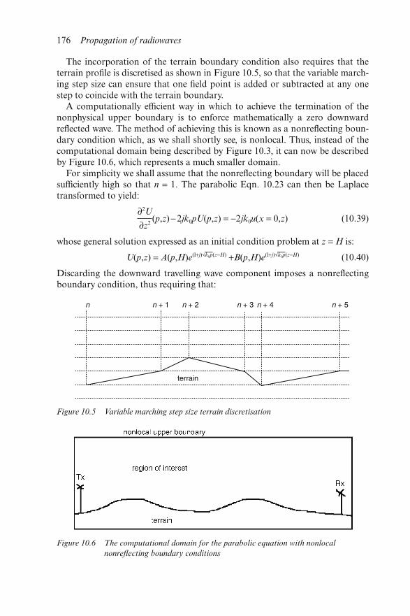
The incorporation of the terrain boundary condition also requires that theterrain profile is discretised as shown in Figure 10.5, so that the variable march-ing step size can ensure that one field point is added or subtracted at any onestep to coincide with the terrain boundary.
A computationally efficient way in which to achieve the termination of thenonphysical upper boundary is to enforce mathematically a zero downwardreflected wave. The method of achieving this is known as a nonreflecting boun-dary condition which, as we shall shortly see, is nonlocal. Thus, instead of thecomputational domain being described by Figure 10.3, it can now be describedby Figure 10.6, which represents a much smaller domain.
For simplicity we shall assume that the nonreflecting boundary will be placedsufficiently high so that n = 1. The parabolic Eqn. 10.23 can then be Laplacetransformed to yield:
∂2U
∂z2(p,z)−2jk0pU(p,z) = −2jk0u(x = 0,z) (10.39)
whose general solution expressed as an initial condition problem at z = H is:
U(p,z) = A(p,H)e(l+j)√k0p(z−H) +B(p,H)e(l+j)√k0p(z−H) (10.40)
Discarding the downward travelling wave component imposes a nonreflectingboundary condition, thus requiring that:
Figure 10.5 Variable marching step size terrain discretisation
Figure 10.6 The computational domain for the parabolic equation with nonlocal
nonreflecting boundary conditions
176 Propagation of radiowaves
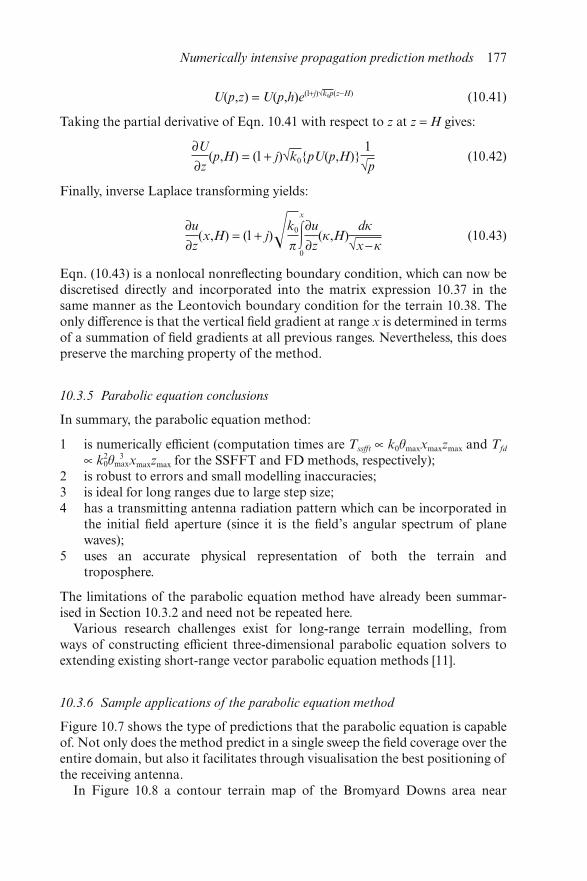
U(p,z) = U(p,h)e(l+j)√k0p(z−H) (10.41)
Taking the partial derivative of Eqn. 10.41 with respect to z at z = H gives:
∂U
∂z(p,H) = (l + j)√k0{pU(p,H)}
1
√p(10.42)
Finally, inverse Laplace transforming yields:
∂u
∂z(x,H) = (l + j)�k0
π�x
0
∂u
∂z(κ,H)
dκ
√x −κ(10.43)
Eqn. (10.43) is a nonlocal nonreflecting boundary condition, which can now bediscretised directly and incorporated into the matrix expression 10.37 in thesame manner as the Leontovich boundary condition for the terrain 10.38. Theonly difference is that the vertical field gradient at range x is determined in termsof a summation of field gradients at all previous ranges. Nevertheless, this doespreserve the marching property of the method.
10.3.5 Parabolic equation conclusions
In summary, the parabolic equation method:
1 is numerically efficient (computation times are Tssfft ∝ k0θmaxxmaxzmax and Tfd
∝ k20θ
3maxxmaxzmax for the SSFFT and FD methods, respectively);
2 is robust to errors and small modelling inaccuracies;3 is ideal for long ranges due to large step size;4 has a transmitting antenna radiation pattern which can be incorporated in
the initial field aperture (since it is the field’s angular spectrum of planewaves);
5 uses an accurate physical representation of both the terrain andtroposphere.
The limitations of the parabolic equation method have already been summar-ised in Section 10.3.2 and need not be repeated here.
Various research challenges exist for long-range terrain modelling, fromways of constructing efficient three-dimensional parabolic equation solvers toextending existing short-range vector parabolic equation methods [11].
10.3.6 Sample applications of the parabolic equation method
Figure 10.7 shows the type of predictions that the parabolic equation is capableof. Not only does the method predict in a single sweep the field coverage over theentire domain, but also it facilitates through visualisation the best positioning ofthe receiving antenna.
In Figure 10.8 a contour terrain map of the Bromyard Downs area near
Numerically intensive propagation prediction methods 177
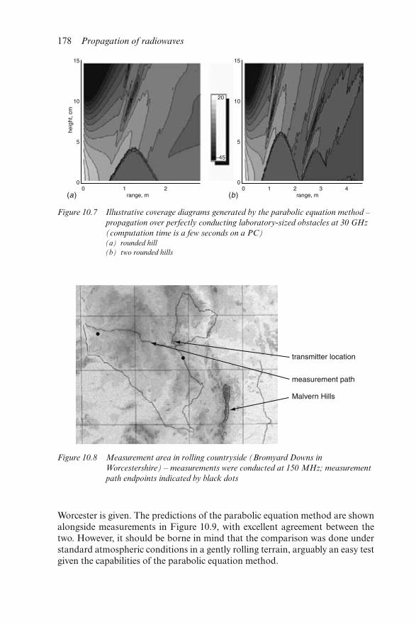
Worcester is given. The predictions of the parabolic equation method are shownalongside measurements in Figure 10.9, with excellent agreement between thetwo. However, it should be borne in mind that the comparison was done understandard atmospheric conditions in a gently rolling terrain, arguably an easy testgiven the capabilities of the parabolic equation method.
Figure 10.7 Illustrative coverage diagrams generated by the parabolic equation method –
propagation over perfectly conducting laboratory-sized obstacles at 30 GHz
(computation time is a few seconds on a PC)(a) rounded hill
(b) two rounded hills
Figure 10.8 Measurement area in rolling countryside (Bromyard Downs in
Worcestershire) – measurements were conducted at 150 MHz; measurement
path endpoints indicated by black dots
178 Propagation of radiowaves
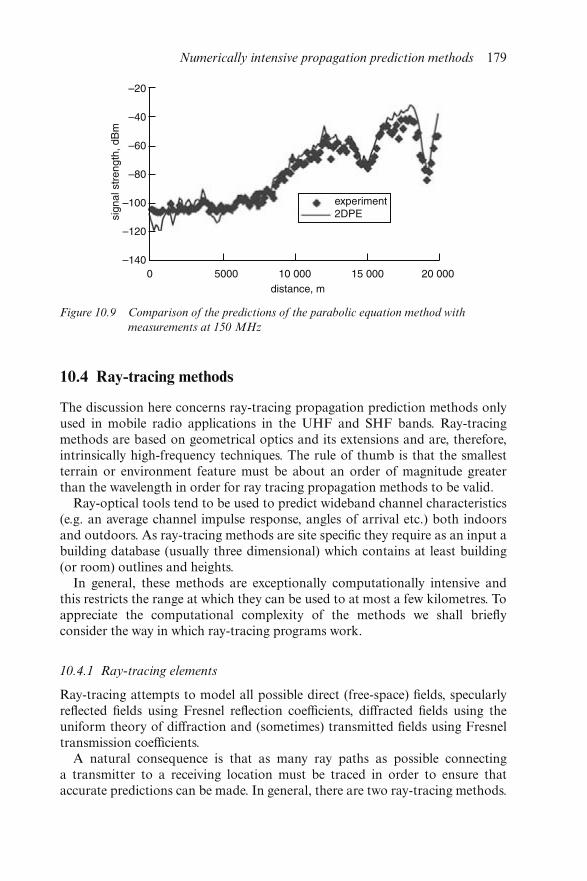
10.4 Ray-tracing methods
The discussion here concerns ray-tracing propagation prediction methods onlyused in mobile radio applications in the UHF and SHF bands. Ray-tracingmethods are based on geometrical optics and its extensions and are, therefore,intrinsically high-frequency techniques. The rule of thumb is that the smallestterrain or environment feature must be about an order of magnitude greaterthan the wavelength in order for ray tracing propagation methods to be valid.
Ray-optical tools tend to be used to predict wideband channel characteristics(e.g. an average channel impulse response, angles of arrival etc.) both indoorsand outdoors. As ray-tracing methods are site specific they require as an input abuilding database (usually three dimensional) which contains at least building(or room) outlines and heights.
In general, these methods are exceptionally computationally intensive andthis restricts the range at which they can be used to at most a few kilometres. Toappreciate the computational complexity of the methods we shall brieflyconsider the way in which ray-tracing programs work.
10.4.1 Ray-tracing elements
Ray-tracing attempts to model all possible direct (free-space) fields, specularlyreflected fields using Fresnel reflection coefficients, diffracted fields using theuniform theory of diffraction and (sometimes) transmitted fields using Fresneltransmission coefficients.
A natural consequence is that as many ray paths as possible connectinga transmitter to a receiving location must be traced in order to ensure thataccurate predictions can be made. In general, there are two ray-tracing methods.
Figure 10.9 Comparison of the predictions of the parabolic equation method with
measurements at 150 MHz
Numerically intensive propagation prediction methods 179
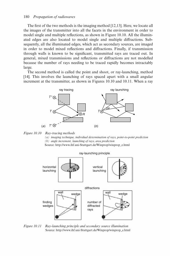
The first of the two methods is the imaging method [12,13]. Here, we locate allthe images of the transmitter into all the facets in the environment in order tomodel single and multiple reflections, as shown in Figure 10.10. All the illumin-ated edges are also located to model single and multiple diffractions. Sub-sequently, all the illuminated edges, which act as secondary sources, are imagedin order to model mixed reflections and diffractions. Finally, if transmissionthrough walls is known to be significant, transmitted rays are traced out. Ingeneral, mixed transmissions and reflections or diffractions are not modelledbecause the number of rays needing to be traced rapidly becomes intractablylarge.
The second method is called the point and shoot, or ray-launching, method[14]. This involves the launching of rays spaced apart with a small angularincrement at the transmitter, as shown in Figures 10.10 and 10.11. When a ray
Figure 10.10 Ray-tracing methods(a) imaging technique, individual determination of rays, point-to-point prediction
(b) angle increment, launching of rays, area prediction
Source: http://www.ihf.uni-Stuttgart.de/Winprop/winprop_e.html
Figure 10.11 Ray-launching principle and secondary source illuminationSource: http://www.ihf.uni-Stuttgart.de/Winprop/winprop_e.html
180 Propagation of radiowaves
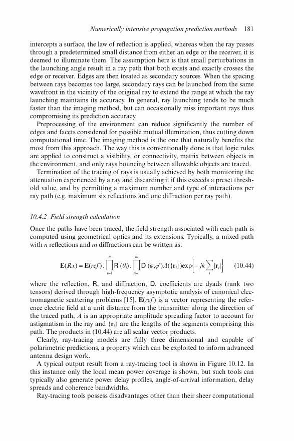
intercepts a surface, the law of reflection is applied, whereas when the ray passesthrough a predetermined small distance from either an edge or the receiver, it isdeemed to illuminate them. The assumption here is that small perturbations inthe launching angle result in a ray path that both exists and exactly crosses theedge or receiver. Edges are then treated as secondary sources. When the spacingbetween rays becomes too large, secondary rays can be launched from the samewavefront in the vicinity of the original ray to extend the range at which the raylaunching maintains its accuracy. In general, ray launching tends to be muchfaster than the imaging method, but can occasionally miss important rays thuscompromising its prediction accuracy.
Preprocessing of the environment can reduce significantly the number ofedges and facets considered for possible mutual illumination, thus cutting downcomputational time. The imaging method is the one that naturally benefits themost from this approach. The way this is conventionally done is that logic rulesare applied to construct a visibility, or connectivity, matrix between objects inthe environment, and only rays bouncing between allowable objects are traced.
Termination of the tracing of rays is usually achieved by both monitoring theattenuation experienced by a ray and discarding it if this exceeds a preset thresh-old value, and by permitting a maximum number and type of interactions perray path (e.g. maximum six reflections and one diffraction per ray path).
10.4.2 Field strength calculation
Once the paths have been traced, the field strength associated with each path iscomputed using geometrical optics and its extensions. Typically, a mixed pathwith n reflections and m diffractions can be written as:
E(Rx) = E(ref ) . n
ν=1
R (θi) . m
μ=1
D (φ,φ′)A({ri})exp�− jk�i
|ri|� (10.44)
where the reflection, R, and diffraction, D, coefficients are dyads (rank twotensors) derived through high-frequency asymptotic analysis of canonical elec-tromagnetic scattering problems [15]. E(ref ) is a vector representing the refer-ence electric field at a unit distance from the transmitter along the direction ofthe traced path, A is an appropriate amplitude spreading factor to account forastigmatism in the ray and {ri} are the lengths of the segments comprising thispath. The products in (10.44) are all scalar vector products.
Clearly, ray-tracing models are fully three dimensional and capable ofpolarimetric predictions, a property which can be exploited to inform advancedantenna design work.
A typical output result from a ray-tracing tool is shown in Figure 10.12. Inthis instance only the local mean power coverage is shown, but such tools cantypically also generate power delay profiles, angle-of-arrival information, delayspreads and coherence bandwidths.
Ray-tracing tools possess disadvantages other than their sheer computational
Numerically intensive propagation prediction methods 181
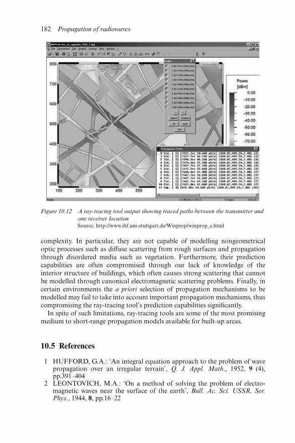
complexity. In particular, they are not capable of modelling nongeometricaloptic processes such as diffuse scattering from rough surfaces and propagationthrough disordered media such as vegetation. Furthermore, their predictioncapabilities are often compromised through our lack of knowledge of theinterior structure of buildings, which often causes strong scattering that cannotbe modelled through canonical electromagnetic scattering problems. Finally, incertain environments the a priori selection of propagation mechanisms to bemodelled may fail to take into account important propagation mechanisms, thuscompromising the ray-tracing tool’s prediction capabilities significantly.
In spite of such limitations, ray-tracing tools are some of the most promisingmedium to short-range propagation models available for built-up areas.
10.5 References
1 HUFFORD, G.A.: ‘An integral equation approach to the problem of wavepropagation over an irregular terrain’, Q. J. Appl. Math., 1952, 9 (4),pp.391–404
2 LEONTOVICH, M.A.: ‘On a method of solving the problem of electro-magnetic waves near the surface of the earth’, Bull. Ac. Sci. USSR, Ser.Phys., 1944, 8, pp.16–22
Figure 10.12 A ray-tracing tool output showing traced paths between the transmitter and
one receiver locationSource: http://www.ihf.uni-stuttgart.de/Winprop/winprop_e.html
182 Propagation of radiowaves
3 WU, Z., and MACLEAN, T.S.M.: ‘Radiowave propagation over groundsoftware’ (Chapman and Hall, London, 1998)
4 LEONTOVICH, M.A. and FOCK, V.: ‘Solution of the problem of elec-tromagnetic waves along the earth’s surface by the method of parabolicequation’, J. Physics (USSR), 1946, 10, pp.13–24
5 TAPPERT, F.D.: ‘The parabolic equation method’, in KELLER, J.B.,and PAPADAKIS, J. (Eds.): ‘Wave propagation and underwater acoustics,Lecture notes in physics, 70’ (Springer, Berlin, 1977)
6 LEE, D., and McDANIEL, S.T.: ‘Ocean acoustic propagation by finitedifference methods’, J. Comp. & Math. With Appl., 1987, 14, pp.305–423
7 KUTTLER, J.R., and DOCKERY, G.D.: ‘Theoretical description of theparabolic approximation/Fourier split-step method of representingelectromagnetic propagation in the troposphere’, Radio Sci., 1991, 26,pp.381–393
8 CRAIG, K.H., and LEVY, M.F.: ‘Parabolic equation modelling of theeffects of multipath and ducting on radar systems’, IEE Proc. F., 1991, 138,pp.153–162
9 BARRIOS, A.E.: ‘A terrain parabolic equation model for propagation inthe troposphere’, IEEE Trans. Antennas Propag., 1994, 42, pp.90–98
10 DOCKERY, G.D., and KUTTLER, J.R.: ‘An improved impedance-boundary algorithm for Fourier split-step solutions of the parabolicequation’, IEEE Trans. Antennas Propag., 1996, 44, pp.1592–1599
11 ZAPOROZHETS, A.A.: ‘Application of the vector parabolic equationmethod to urban radiowave propagation problems’, IEE Proc. H, 1999, 146,pp.253–256
12 IKEGAMI, F., TAKEUCHI, T., and YOSHIDA, S.: ‘Theoretical predic-tion of mean field strength for urban mobile radio’, IEEE Trans. AntennasPropag., 1991, 39, pp.299–302
13 ROSSI, J.-P., and LEVY, A.J.: ‘A ray model for decimetric radiowavepropagation in an urban area’, Radio Sci., 1992, 27, pp.971–979
14 LUEBBERS, R., and SCHUSTER, J.: ‘Site-specific propagation predictionmethods for urban environments’. AGARD CP-574, 1995, pp.41.1–12
15 HANSEN, R.C. (Ed.): ‘Geometric theory of diffraction’ (IEEE Press, NewYork, 1981)
Numerically intensive propagation prediction methods 183

Chapter 11
Outdoor mobile propagation
Simon R. Saunders
11.1 Introduction
This Chapter describes key modelling concepts for mobile communication sys-tems operated in outdoor environments. Much of the content is adapted fromSaunders [1], to which the reader is referred for further detail.
Figure 11.1 shows a few of the many interactions between electromagneticwaves, the antennas which launch and receive them and the environmentthrough which they propagate, in order to understand outdoor mobile propaga-tion. Sometimes these effects are treated using detailed physical models, butmore usually they are considered too complex and are treated in an empirical orstatistical manner. This Chapter examines how these effects are modelled formacrocells and microcells, which together comprise the main system types usedin cellular mobile communications.
11.1.1 The outdoor mobile radio channel
The outdoor mobile channel is a special case of the channel defined for genericcommunication systems by Shannon [2]. The transmitted information, encodedas suitable waveforms by the transmitter, is modified by channel noise in wayswhich may be more or less unpredictable to the receiver, so the receiver must bedesigned to overcome these modifications and hence to deliver the informationto its final destination with as few errors or distortions as possible.
In the wireless channel, the noise sources can be subdivided into multiplicativeand additive effects. The additive noise arises from noise generated within thereceiver itself, such as thermal and shot noise in passive and active devices andalso from external sources particularly interference from other transmitters andelectrical systems. Some of this interference may be intentionally introduced,but carefully controlled, such as when channels are reused in order to maximisethe capacity of a cellular radio system.
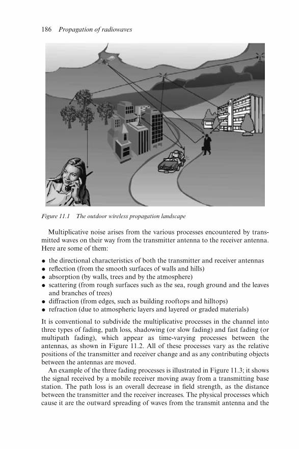
Multiplicative noise arises from the various processes encountered by trans-mitted waves on their way from the transmitter antenna to the receiver antenna.Here are some of them:
• the directional characteristics of both the transmitter and receiver antennas
• reflection (from the smooth surfaces of walls and hills)
• absorption (by walls, trees and by the atmosphere)
• scattering (from rough surfaces such as the sea, rough ground and the leavesand branches of trees)
• diffraction (from edges, such as building rooftops and hilltops)
• refraction (due to atmospheric layers and layered or graded materials)
It is conventional to subdivide the multiplicative processes in the channel intothree types of fading, path loss, shadowing (or slow fading) and fast fading (ormultipath fading), which appear as time-varying processes between theantennas, as shown in Figure 11.2. All of these processes vary as the relativepositions of the transmitter and receiver change and as any contributing objectsbetween the antennas are moved.
An example of the three fading processes is illustrated in Figure 11.3; it showsthe signal received by a mobile receiver moving away from a transmitting basestation. The path loss is an overall decrease in field strength, as the distancebetween the transmitter and the receiver increases. The physical processes whichcause it are the outward spreading of waves from the transmit antenna and the
Figure 11.1 The outdoor wireless propagation landscape
186 Propagation of radiowaves
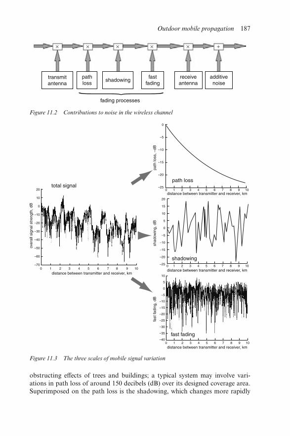
obstructing effects of trees and buildings; a typical system may involve vari-ations in path loss of around 150 decibels (dB) over its designed coverage area.Superimposed on the path loss is the shadowing, which changes more rapidly
Figure 11.2 Contributions to noise in the wireless channel
Figure 11.3 The three scales of mobile signal variation
Outdoor mobile propagation 187
with significant variations over distances of hundreds of metres and generallyinvolves variations of up to around 20 dB. Shadowing arises due to the varyingnature of the particular obstructions between the base and the mobile, such asparticular tall buildings or dense woods. Fast fading involves variations on thescale of a half wavelength (50 cm at 300 MHz, 17 cm at 900 MHz) and fre-quently introduces variations as large as 35 to 40 dB. It results from the con-structive and destructive interference between multiple waves reaching themobile from the base station. In this Chapter only the path loss and shadowingfor outdoor terrestrial mobile systems will be examined. These are the keyvariations for predicting area coverage for practical systems.
Most outdoor mobile propagation occurs at VHF and above. The corres-ponding wavelengths, of the order of metres or less, are shorter than thecritical dimensions of most objects encountered, such as hills or buildings. Thisallows the application of various high-frequency approximations to simplify theanalysis of propagation effects.
11.1.2 System types
This Chapter covers two main outdoor system types, namely macrocells andmicrocells.
(i) Macrocells (Section 11.2): designed to provide mobile services (includingboth voice and paging), particularly outdoors, to rural, suburban andurban environments with medium traffic densities. Base station antennaheights are greater than the surrounding buildings, providing a cell radiusfrom around 1 km to many tens of kilometres. Mostly operated at VHFand UHF.
(ii) Microcells (Section 11.4): designed for high traffic densities in urban andsuburban areas to users both outdoors and within buildings. Base stationantennas are lower than nearby building rooftops, so coverage area is definedby street layout. Cell length up to around 500 m. Again, mostly operated atVHF and UHF, but services as high as 60 GHz have been proposed.
Several other system types are examined in depth in Saunders [1].
11.2 Macrocells
11.2.1 Introduction
This Section introduces methods for predicting the path loss encountered inmacrocells. In principle, wave propagation could be analysed in detail to predictthe loss over every path between the base station and every possible mobilelocation. However, the data describing the terrain and clutter would be verylarge and the computational effort involved would often be excessive. Even ifsuch resources were available, the important parameter for the macrocelldesigner is the overall area covered, rather than the specific field strength atparticular locations.
188 Propagation of radiowaves
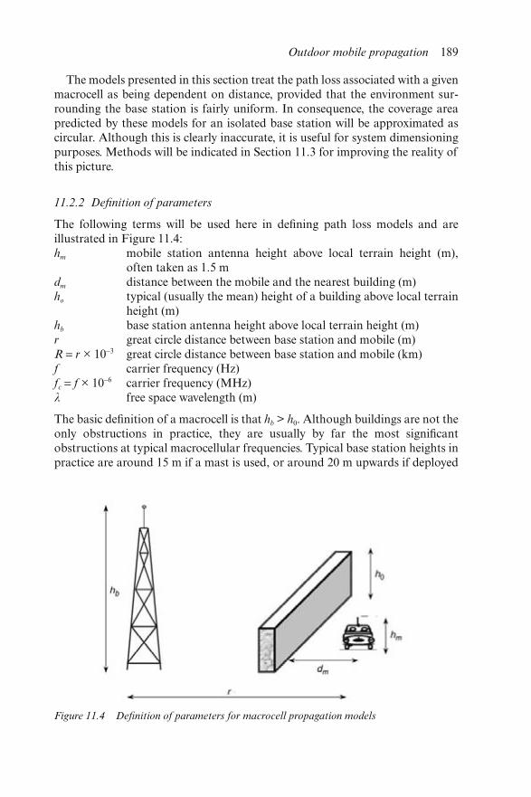
The models presented in this section treat the path loss associated with a givenmacrocell as being dependent on distance, provided that the environment sur-rounding the base station is fairly uniform. In consequence, the coverage areapredicted by these models for an isolated base station will be approximated ascircular. Although this is clearly inaccurate, it is useful for system dimensioningpurposes. Methods will be indicated in Section 11.3 for improving the reality ofthis picture.
11.2.2 Definition of parameters
The following terms will be used here in defining path loss models and areillustrated in Figure 11.4:hm mobile station antenna height above local terrain height (m),
often taken as 1.5 mdm distance between the mobile and the nearest building (m)ho typical (usually the mean) height of a building above local terrain
height (m)hb base station antenna height above local terrain height (m)r great circle distance between base station and mobile (m)R = r × 10−3 great circle distance between base station and mobile (km)f carrier frequency (Hz)fc = f × 10−6 carrier frequency (MHz)λ free space wavelength (m)
The basic definition of a macrocell is that hb > h0. Although buildings are not theonly obstructions in practice, they are usually by far the most significantobstructions at typical macrocellular frequencies. Typical base station heights inpractice are around 15 m if a mast is used, or around 20 m upwards if deployed
Figure 11.4 Definition of parameters for macrocell propagation models
Outdoor mobile propagation 189
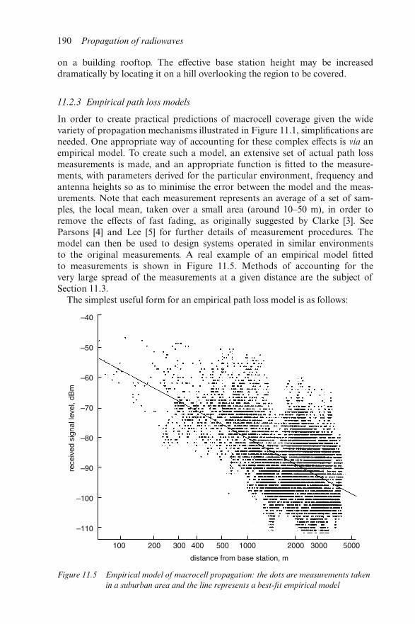
on a building rooftop. The effective base station height may be increaseddramatically by locating it on a hill overlooking the region to be covered.
11.2.3 Empirical path loss models
In order to create practical predictions of macrocell coverage given the widevariety of propagation mechanisms illustrated in Figure 11.1, simplifications areneeded. One appropriate way of accounting for these complex effects is via anempirical model. To create such a model, an extensive set of actual path lossmeasurements is made, and an appropriate function is fitted to the measure-ments, with parameters derived for the particular environment, frequency andantenna heights so as to minimise the error between the model and the meas-urements. Note that each measurement represents an average of a set of sam-ples, the local mean, taken over a small area (around 10–50 m), in order toremove the effects of fast fading, as originally suggested by Clarke [3]. SeeParsons [4] and Lee [5] for further details of measurement procedures. Themodel can then be used to design systems operated in similar environmentsto the original measurements. A real example of an empirical model fittedto measurements is shown in Figure 11.5. Methods of accounting for thevery large spread of the measurements at a given distance are the subject ofSection 11.3.
The simplest useful form for an empirical path loss model is as follows:
Figure 11.5 Empirical model of macrocell propagation: the dots are measurements taken
in a suburban area and the line represents a best-fit empirical model
190 Propagation of radiowaves
PR
PT
= 1
L =
k
rn or in decibels L = 10n log r + K (11.1)
where PT and PR are the effective transmitted and predicted isotropic receivedpowers, L is the path loss, r is the distance between the base station and themobile and K = 10 log10k and n are constants of the model. This will be referredto as a power law model. A more convenient form (in decibels) is
L = 10n log(r/rref) + Lref (11.2)
where Lref is the predicted loss at a reference distance rref.Both the free-space loss and the plane earth loss can be expressed in this form.
The parameter n is known as the path loss exponent and is found by measure-ment to depend on the system parameters, such as antenna heights and theenvironment. The path loss exponent is critical in establishing the coverage andcapacity of a cellular system. Parameter k can be considered as the reciprocal ofthe propagation loss that would be experienced at one metre range (r = 1 m).
11.2.3.1 Clutter factor models
Measurements taken in urban and suburban areas usually find a path lossexponent close to 4, just as in the plane earth loss but with a greater absolute lossvalue – smaller K in Eqn. 11.1. This has led to some models being proposedwhich consist of the plane earth loss (see Chapter 6), plus (in decibels) an extraloss component called the clutter factor, as shown in Figure 11.6. The variousmodels differ basically in the values which they assign to k and n for differentfrequencies and environments.
A good example of a clutter factor model is the method due to Egli [6], whichis based upon a large number of measurements taken around American cities.Egli’s overall results were originally presented in nomograph form, but Delisle[7] has given an approximation to these results for easier computation:
L = 40 log R + 20 log fc − 20 log hb + Lm (11.3)
where
Lm = 76.3 − 10 log hm for hm <10
(11.4)76.3 − 20 log hm for hm ≥10
⎧⎨⎩
Note that this approximation (Eqn. 11.4) involves a small discontinuity athm = 10 m. Although plane earth loss is frequency independent, this model intro-duces an additional f −2
c received power dependence, which is more representa-tive of the results of real measurements. For very large antenna heights, theloss predicted by Eqn. 11.3 may be less than the free-space value, in which casethe free-space value is used.
The mobile antenna height-gain characteristic is approximately linear forantennas which clear the surrounding terrain features, assumed to be above10 m. Elsewhere there is a square root variation for heights in the range
Outdoor mobile propagation 191
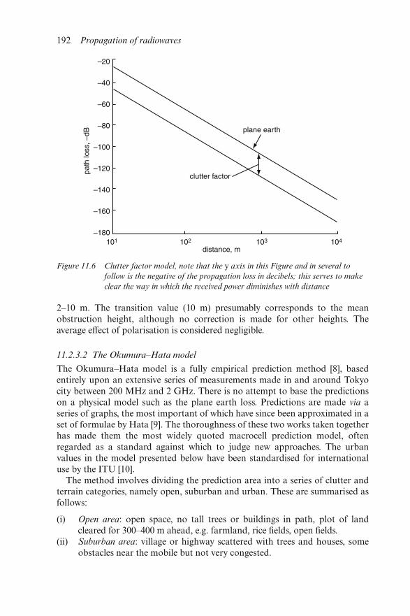
2–10 m. The transition value (10 m) presumably corresponds to the meanobstruction height, although no correction is made for other heights. Theaverage effect of polarisation is considered negligible.
11.2.3.2 The Okumura–Hata model
The Okumura–Hata model is a fully empirical prediction method [8], basedentirely upon an extensive series of measurements made in and around Tokyocity between 200 MHz and 2 GHz. There is no attempt to base the predictionson a physical model such as the plane earth loss. Predictions are made via aseries of graphs, the most important of which have since been approximated in aset of formulae by Hata [9]. The thoroughness of these two works taken togetherhas made them the most widely quoted macrocell prediction model, oftenregarded as a standard against which to judge new approaches. The urbanvalues in the model presented below have been standardised for internationaluse by the ITU [10].
The method involves dividing the prediction area into a series of clutter andterrain categories, namely open, suburban and urban. These are summarised asfollows:
(i) Open area: open space, no tall trees or buildings in path, plot of landcleared for 300–400 m ahead, e.g. farmland, rice fields, open fields.
(ii) Suburban area: village or highway scattered with trees and houses, someobstacles near the mobile but not very congested.
Figure 11.6 Clutter factor model, note that the y axis in this Figure and in several to
follow is the negative of the propagation loss in decibels; this serves to make
clear the way in which the received power diminishes with distance
192 Propagation of radiowaves
(iii) Urban area: built-up city or large town with large buildings and houseswith two or more storeys, or larger villages with close houses and tall,thickly grown trees.
Okumura takes urban areas as a reference and applies correction factors forconversion to the other classifications. This is a sensible choice, since such areasavoid the large variability present in suburban areas (see Chapter 9) and yetinclude the effects of obstructions better than could be done with open areas. Aseries of terrain types is also defined for when such information is available.Quasi-smooth terrain is taken as the reference and correction factors are addedfor the other types of terrain.
Okumura’s predictions of median path loss are usually calculated usingHata’s approximations as follows [9]:
urban areas LdB = A + B log R − Esuburban areas LdB = A + B log R − C (11.5)open areas LdB = A + B log R − D
where
A = 69.55 + 26.16 log fc − 13.82 log hb
B = 44.9 − 6.55 log hb
C = 2(log(fc/28))2 + 5.4(11.6)D = 4.78(log fc)
2 + 18.33 log fc + 40.94E = 3.2 (log(11.75 hm))2 − 4.97 for large cities, fc ≥ 300 MHzE = 8.29 (log(1.54 hm))2 − 1.1 for large cities, fc < 300 MHzE = (1.1 log fc − 0.7)hm − (1.56 log fc − 0.8) for medium to small cities
The model is valid only for 150 MHz ≤ fc ≤ 1500 MHz, 30 m ≤ hb ≤ 200 m,1 m < hm < 10 m and R > 1 km. The path loss exponent is given by B/10, whichis a little less than 4, decreasing with increasing base station antenna height.
Base station antenna height hb is defined as the height above the averageground level in the range 3–10 km from the base station; hb may therefore varyslightly with the direction of the mobile from the base. The height gain factorvaries between 6 dB octave−1 and 9 dB octave−1 as the height increases from 30 mto 1 km. Measurements also suggest that this factor depends upon range.
Okumura found that mobile antenna height gain is 3 dB octave−1 up to hm = 3 mand 8 dB octave−1 beyond. It depends partially upon urban density, apparentlyas a result of the effect of building heights on the angle-of-arrival of wave energyat the mobile and the consequent shadow loss variation. Urban areas are there-fore subdivided into large cities and medium/small cities, where an area havingan average building height in excess of 15 m is defined as a large city.
Other correction factors are included in Okumura’s original work for theeffects of street orientation (if an area has a large proportion of streets whichare either radial or tangential to the propagation direction) and a fine correctionfor rolling hilly terrain (used if a large proportion of streets are placed at eitherthe peaks or valleys of the terrain undulations). Application of the method
Outdoor mobile propagation 193
involves first finding the basic median field strength in concentric circles aroundthe base station, then amending them according to the terrain and cluttercorrection graphs.
Okumura’s predictions have been found useful in many cases [11], par-ticularly in suburban areas. However, other measurements have been indisagreement with these predictions; the reasons for error are often cited asthe difference in the characteristics of the area under test with Tokyo. Otherauthors such as Kozono [12] have attempted to modify Okumura’s methodto include a measure of building density, but such approaches have not foundcommon acceptance.
The Okumura–Hata model, together with related corrections, is probablythe single most common model used in designing real systems. Several com-mercial prediction tools essentially rely on variations of this model, optimisedfor the particular environments they are catering for, as the basis of theirpredictions.
11.2.3.3 The COST 231–Hata model
The Okumura–Hata model for medium to small cities has been extended tocover the band 1500 MHz < fc < 2000 MHz [13]:
LdB = F + B log R − E + G (11.7)
where
F = 46.3 + 33.9 log fc − 13.82 log hb (11.8)
E is as defined in Eqn. 11.6 for medium to small cities and
G = 0 dB medium-sized cities and suburban areas (11.9)
3 dB metropolitan areas
⎧⎨⎩
11.2.3.4 Environment categories
In an empirical model, it is crucial to correctly classify the environment in whichthe system is operating. The models assume that the characteristics of theenvironment to be predicted are sufficiently similar to those where the originalmeasurements were taken that the propagation loss at a given distance will besimilar. Good results will therefore only be obtained if the correct classificationis chosen. The categories of environment should also be sufficiently numerousthat the properties of different locations classed within the same category arenot too variable. The decision as to which category an environment fits into isusually purely subjective and may vary between individuals and countries. Forexample, the Okumura–Hata model uses four categories: large cities, medium-small cities, suburban areas and open areas. Since the original measurementswere made in Tokyo, the model relies on other parts of the world having charac-teristics which are somehow similar to those in Tokyo. Although this is an
194 Propagation of radiowaves
extremely questionable assumption, it is nevertheless true that the model hasbeen applied to many successful system designs.
Many more detailed schemes exist for qualitative classification of land usage.Schemes often correspond to sources of data, such as satellite remote-sensingdata which classifies land according to the degree of scattering experienced atvarious wavelengths. This at least avoids the need for ambiguous judgements tobe made. Nevertheless, there is no guarantee that there is any one-to-one map-ping between the propagation characteristics and such measures of land usage.In order to find more appropriate parameters, the growing tendency in macrocel-lular propagation is towards models which have a physical basis, and these areexamined in the next section.
11.2.4 Physical models
Although empirical models have been extensively applied with good results, theysuffer from a number of disadvantages:
• they can only be used over parameter ranges included in the originalmeasurement set;
• environments must be classified subjectively according to categories such asurban, which have different meanings in different countries;
• they provide no physical insight into the mechanisms by which propagationoccurs.
The last point is particularly significant, as empirical models are unable toaccount for factors such as an unusually large building or hill which may greatlymodify propagation in particular locations.
Although the plane earth model has a path loss exponent close to thatobserved in actual measurements (i.e. 4), the simple physical situation itdescribes is rarely applicable in practice. The mobile is almost always operated(at least in macrocells) in situations where it does not have a line-of-sight path toeither the base station or to the ground reflection point, so the two-ray situationwhich the plane earth model relies upon is hardly ever applicable. In order tofind a more satisfactory physical propagation model, we examine diffraction as apotential mechanism.
11.2.4.1 The Ikegami model
This model attempts to produce an entirely deterministic prediction of fieldstrengths at specified points [14]. Using a detailed map of building heights,shapes and positions, ray paths between the transmitter and receiver are traced,with the restriction that only single reflections from walls are accounted for.Diffraction is calculated using a single edge approximation at the building near-est the mobile, and wall reflection loss is assumed to be fixed at a constant value.The two rays (reflected and diffracted) are power summed, resulting in thefollowing approximate model:
Outdoor mobile propagation 195
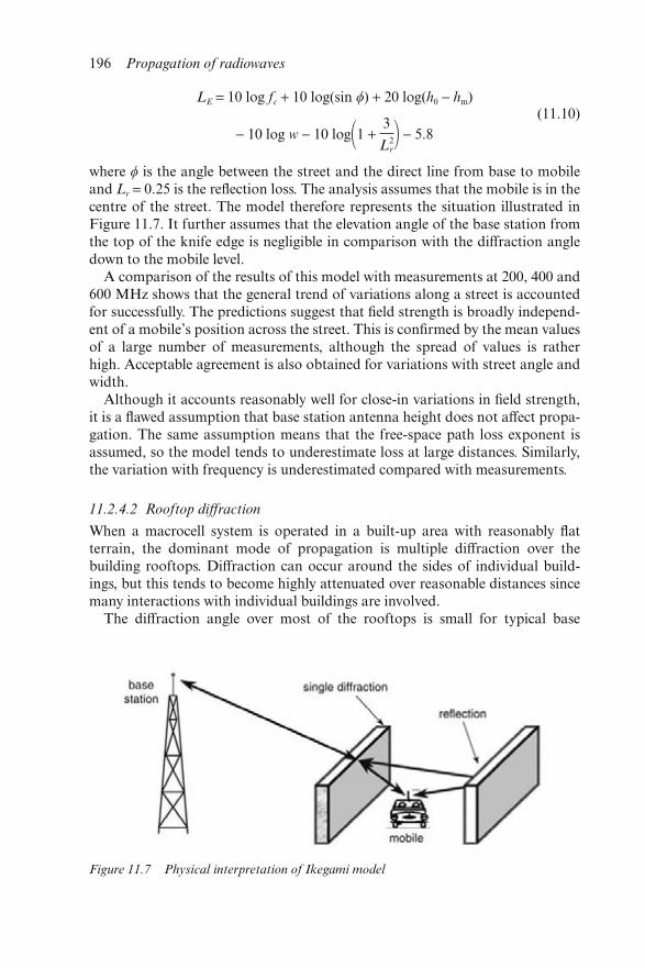
LE = 10 log fc + 10 log(sin ) + 20 log(h0 − hm)
− 10 log w − 10 log�1 + 3
L2r� − 5.8
(11.10)
where is the angle between the street and the direct line from base to mobileand Lr = 0.25 is the reflection loss. The analysis assumes that the mobile is in thecentre of the street. The model therefore represents the situation illustrated inFigure 11.7. It further assumes that the elevation angle of the base station fromthe top of the knife edge is negligible in comparison with the diffraction angledown to the mobile level.
A comparison of the results of this model with measurements at 200, 400 and600 MHz shows that the general trend of variations along a street is accountedfor successfully. The predictions suggest that field strength is broadly independ-ent of a mobile’s position across the street. This is confirmed by the mean valuesof a large number of measurements, although the spread of values is ratherhigh. Acceptable agreement is also obtained for variations with street angle andwidth.
Although it accounts reasonably well for close-in variations in field strength,it is a flawed assumption that base station antenna height does not affect propa-gation. The same assumption means that the free-space path loss exponent isassumed, so the model tends to underestimate loss at large distances. Similarly,the variation with frequency is underestimated compared with measurements.
11.2.4.2 Rooftop diffraction
When a macrocell system is operated in a built-up area with reasonably flatterrain, the dominant mode of propagation is multiple diffraction over thebuilding rooftops. Diffraction can occur around the sides of individual build-ings, but this tends to become highly attenuated over reasonable distances sincemany interactions with individual buildings are involved.
The diffraction angle over most of the rooftops is small for typical base
Figure 11.7 Physical interpretation of Ikegami model
196 Propagation of radiowaves
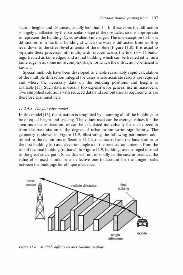
station heights and distances, usually less than 1°. In these cases the diffractionis largely unaffected by the particular shape of the obstacles, so it is appropriateto represent the buildings by equivalent knife edges. The one exception to this isdiffraction from the final building at which the wave is diffracted from rooftoplevel down to the street-level antenna of the mobile (Figure 11.8). It is usual toseparate these processes into multiple diffraction across the first (n − 1) build-ings, treated as knife edges, and a final building which can be treated either as aknife edge or as some more complex shape for which the diffraction coefficient isknown.
Special methods have been developed to enable reasonably rapid calculationof the multiple diffraction integral for cases where accurate results are requiredand where the necessary data on the building positions and heights isavailable [15]. Such data is usually too expensive for general use in macrocells.Two simplified solutions with reduced data and computational requirements aretherefore examined here.
11.2.4.3 The flat edge model
In this model [16], the situation is simplified by assuming all of the buildings tobe of equal height and spacing. The values used can be average values for thearea under consideration, or can be calculated individually for each directionfrom the base station if the degree of urbanisation varies significantly. Thegeometry is shown in Figure 11.9, illustrating the following parameters add-itional to the definitions in Section 11.2.2, distance r1 from the base station tothe first building (m) and elevation angle α of the base station antenna from thetop of the final building (radians). In Figure 11.9, buildings are arranged normalto the great circle path. Since this will not normally be the case in practice, thevalue of w used should be an effective one to account for the longer pathsbetween the buildings for oblique incidence.
Figure 11.8 Multiple diffraction over building rooftops
Outdoor mobile propagation 197
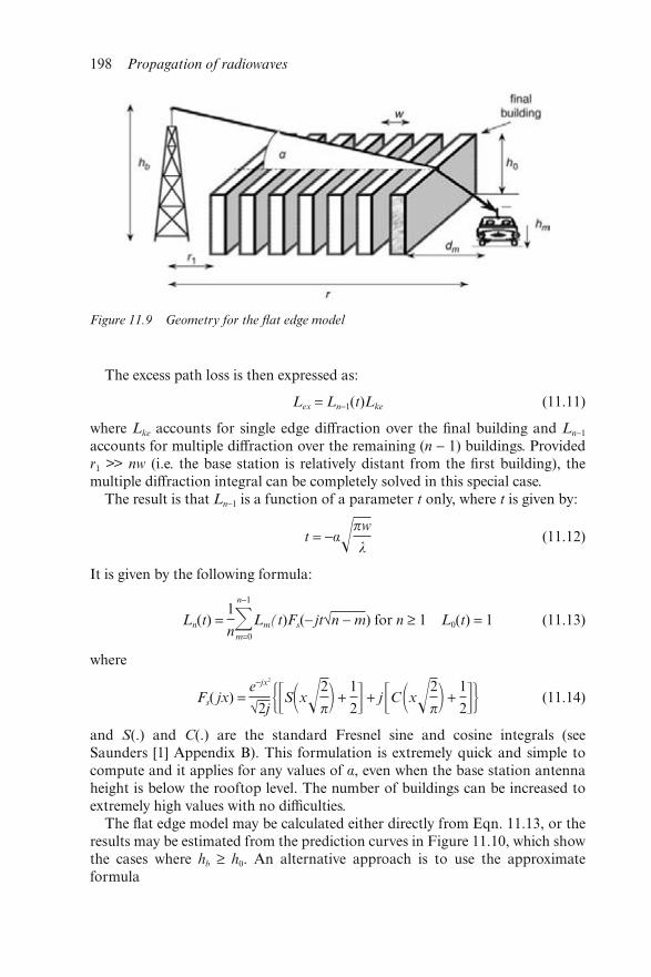
The excess path loss is then expressed as:
Lex = Ln−1(t)Lke (11.11)
where Lke accounts for single edge diffraction over the final building and Ln−1
accounts for multiple diffraction over the remaining (n − 1) buildings. Providedr1 >> nw (i.e. the base station is relatively distant from the first building), themultiple diffraction integral can be completely solved in this special case.
The result is that Ln−1 is a function of a parameter t only, where t is given by:
t = −α�πw
λ(11.12)
It is given by the following formula:
Ln(t) = 1
n�n−1
m=0
Lm(t)Fs(− jt√n − m) for n ≥ 1 L0(t) = 1 (11.13)
where
Fs( jx) = e−jx2
√2j �S�x�2
π� + 1
2� + j C �x�2
π� + 1
2�� (11.14)
and S(.) and C(.) are the standard Fresnel sine and cosine integrals (seeSaunders [1] Appendix B). This formulation is extremely quick and simple tocompute and it applies for any values of α, even when the base station antennaheight is below the rooftop level. The number of buildings can be increased toextremely high values with no difficulties.
The flat edge model may be calculated either directly from Eqn. 11.13, or theresults may be estimated from the prediction curves in Figure 11.10, which showthe cases where hb ≥ h0. An alternative approach is to use the approximateformula
Figure 11.9 Geometry for the flat edge model
198 Propagation of radiowaves
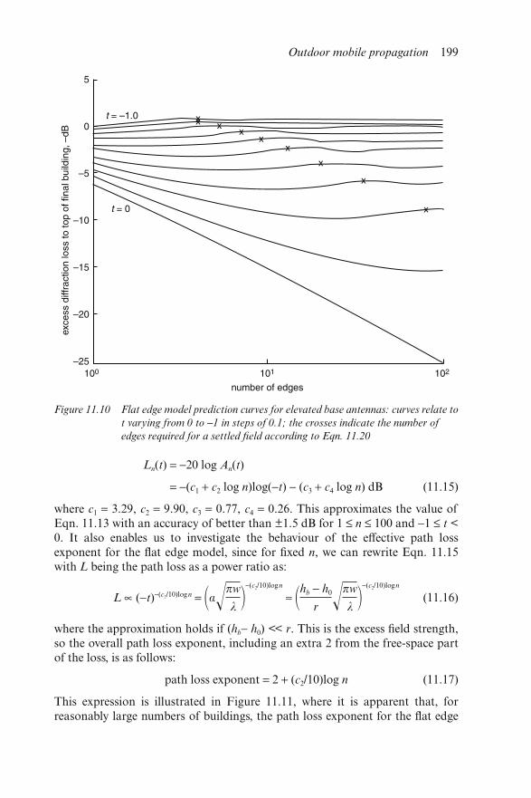
Ln(t) = −20 log An(t)
= −(c1 + c2 log n)log(−t) − (c3 + c4 log n) dB (11.15)
where c1 = 3.29, c2 = 9.90, c3 = 0.77, c4 = 0.26. This approximates the value ofEqn. 11.13 with an accuracy of better than ±1.5 dB for 1 ≤ n ≤ 100 and −1 ≤ t <0. It also enables us to investigate the behaviour of the effective path lossexponent for the flat edge model, since for fixed n, we can rewrite Eqn. 11.15with L being the path loss as a power ratio as:
L ∝ (−t)−(c2/10)logn = �α�πw
λ �−(c2/10)logn
≈ �hb − h0
r �πw
λ �−(c2/10)logn
(11.16)
where the approximation holds if (hb− h0) << r. This is the excess field strength,so the overall path loss exponent, including an extra 2 from the free-space partof the loss, is as follows:
path loss exponent = 2 + (c2/10)log n (11.17)
This expression is illustrated in Figure 11.11, where it is apparent that, forreasonably large numbers of buildings, the path loss exponent for the flat edge
Figure 11.10 Flat edge model prediction curves for elevated base antennas: curves relate to
t varying from 0 to −1 in steps of 0.1; the crosses indicate the number of
edges required for a settled field according to Eqn. 11.20
Outdoor mobile propagation 199
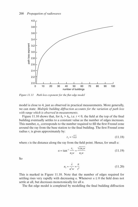
model is close to 4, just as observed in practical measurements. More generally,we can state: Multiple building diffraction accounts for the variation of path loss
with range which is observed in measurements.Figure 11.10 shows that, for hb > h0, i.e. t < 0, the field at the top of the final
building eventually settles to a constant value as the number of edges increases.This number, ns, corresponds to the number required to fill the first Fresnel zonearound the ray from the base station to the final building. The first Fresnel zoneradius r1 is given approximately by:
r1 = √λs (11.18)
where s is the distance along the ray from the field point. Hence, for small α:
α = tan−1 r1
nsw ≈
√λnsw
nsw(11.19)
So
ns ≈ λ
α2w =
π
t2(11.20)
This is marked in Figure 11.10. Note that the number of edges required forsettling rises very rapidly with decreasing α. Whenever α ≤ 0 the field does notsettle at all, but decreases monotonically for all n.
The flat edge model is completed by modelling the final building diffraction
Figure 11.11 Path loss exponent for the flat edge model
200 Propagation of radiowaves
loss and the reflections from the buildings across the street using the Ikegamimodel from Section 11.2.4.1. Thus the total path loss is given by:
LT = Ln(t) + LF + LE (11.21)
where Ln(t) can be found from Eqn. 11.13, Figure 11.10 or Eqn. 11.15, LF is thefree space loss (2.7) and LE is given in Eqn. 11.10.
11.2.4.4 The Walfisch–Bertoni model
This model can be considered as the limiting case of the flat edge model whenthe number of buildings is sufficient for the field to settle, i.e. n ≥ ns. The multiplediffraction process was investigated by Walfisch and Bertoni [17] using a numer-ical evaluation of the Kirchhoff–Huygens integral and a power law formula isfitted to the results for the settled field. The Walfisch–Bertoni model was thefirst to actually demonstrate that multiple building diffraction accounts for thevariation of distance with range which is observed in measurements.
The settled field approximation is as follows:
Asettled(t) ≈ 0.1 � α
0.03�w
λ�0.9
= 0.1 � −t
0.03�0.9
(11.22)
This is only valid for 0.03 ≤ t ≤ 0.4. For large ranges, we can again put:
t ≈ −α�πw
λ ≈ −
hb − hm
r �πw
λ(11.23)
Hence Lsettled ∝ r−1.8. The free-space loss is proportional to r−2, so this modelpredicts that the total propagation loss is proportional to r−3.8, which is closeto the r−4 law which is commonly assumed in empirical models and found inmeasurements. A single knife-edge approximation with a reflection from thebuilding opposite is again used, just as in the Ikegami model, to account forthe diffraction from the final building. The complete model is expressed as:
Lex = 57.1 + LA + log fc + 18 log R − 18 log(hb − h0)
− 18 log1 − R2
17(hb − h0)� (11.24)
where
LA = 5 log�w2� + (h0 − hm)2� − 9 log w
+ 20 log�tan−1 2(h0 − hm)
w �� (11.25)
The use of the settled field approximation requires that large numbers of build-ings are present, particularly when α is small. Despite this limitation, theWalfisch–Bertoni model is the first to have accounted for observed path loss
Outdoor mobile propagation 201
variation using realistic physical assumptions rather than relying upon forcingagreement using propagation models of entirely different situations.
11.2.4.5 COST 231 / Walfisch–Ikegami model
The Walfisch–Bertoni model for the settled field has been combined with theIkegami model for diffraction down to street level and some empirical correctionfactors to improve agreement with measurements in a single integrated model bythe COST 231 project [13].
For nonline-of-sight conditions the total loss is given by:
L = LF + Lmsd + Lsd (11.26)
where LF is the free space loss, Lmsd accounts for multiple knife-edge diffractionto the top of the final building and Lsd accounts for the single diffraction andscattering process down to street level. L is given a minimum value of LF in casethe other terms become negative. The individual terms are:
Lsd = −16.9 + 10 log fc + 10 log (h0 − hm)2
wm
+ L() (11.27)
where wm is the distance between the building faces on either side of the streetcontaining the mobile (typically wm = w/2), and the final term accounts for streetorientation at an angle to the great circle path:
− 10 + 0.354 for 0° < < 35°
L() = 2.5 + 0.075( − 35°) for 35° ≤ < 55° (11.28)
4.0 + 0.114( − 55°) for 55° ≤ < 90°
⎧⎭⎫⎩
Finally, the rooftop diffraction term is given by
Lmsd = Lbsh + ka + kd log R + kf log fc − 9 log w (11.29)
where
Lbsh = �−18 log[1 + (hb − h0)]
0
for hb > h0
for hb ≤ h0
(11.30)
54 for hb > h0
ka = 54 − 0.8(hb − h0) for R ≥ 0.5 km and hb ≤ h0 (11.31)
54 − 0.8(hb − h0)R
0.5for R < 0.5 km and hb ≤ h0
⎧⎪⎨⎪⎩
kd =18
18 − 15(hb − h0)
h0
for hb > h0
for hb ≤ h0(11.32)
⎧⎨⎩
202 Propagation of radiowaves
kf = −4 + 0.7� fc
925 − 1� for medium-sized city and
suburban areas with medium tree density (11.33)
kf = −4 + 1.5� fc
925 − 1� for metropolitan centres
For approximate work, the following parameter values can be used:
h0 = � 3nfloors
3nfloors + 3
for flat roofs
for pitched roofs(11.34)
w = 20 − 50 m, dm = w/2, = 90°
where nfloors is the number of floors in the building. The model is applicablefor 800 MHz ≤ fc ≤ 2000 MHz, 4 m ≤ hb ≤ 50 m, 1 m ≤ hm ≤ 3 m and0.02 km ≤ R ≤ 5 km.
An alternative approach is to replace the Lmsd term by Ln(t) from the flat edgemodel. This would enable the path loss exponent to vary according to the num-ber of buildings and to be uniformly valid for hb ≤ h0. Note, however, that forvery low base station antennas other propagation mechanisms, such as diffrac-tion around vertical building edges and multiple reflections from building walls,are likely to be significant.
11.2.5 Computerised planning tools
The methods described in this Chapter are most often implemented for practicalplanning within computer software. The development of such software has beenmotivated and enabled by a number of factors:
• the enormous increase in the need to plan cellular systems accurately andquickly
• the development of fast, affordable computing resources
• the development of geographical information systems, which index data onterrain, clutter and land usage in an easily accessible and manipulable form.
Such techniques have been implemented in a wide range of commercially avail-able and company-specific planning tools. Although most are based on com-bined empirical and simple physical models, it is anticipated that there will beprogressive evolution in the future towards more physical or physical–statisticalmethods as computing resources continue to cheapen, clutter data improves inresolution and cost and as research develops into numerically efficient path lossprediction algorithms
11.2.6 Conclusions
The accuracy of the path loss predictions is crucial in determining whether aparticular mobile system design will be viable. In macrocells, empirical models
Outdoor mobile propagation 203
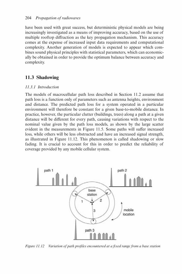
have been used with great success, but deterministic physical models are beingincreasingly investigated as a means of improving accuracy, based on the use ofmultiple rooftop diffraction as the key propagation mechanism. This accuracycomes at the expense of increased input data requirements and computationalcomplexity. Another generation of models is expected to appear which com-bines sound physical principles with statistical parameters, which can economic-ally be obtained in order to provide the optimum balance between accuracy andcomplexity.
11.3 Shadowing
11.3.1 Introduction
The models of macrocellular path loss described in Section 11.2 assume thatpath loss is a function only of parameters such as antenna heights, environmentand distance. The predicted path loss for a system operated in a particularenvironment will therefore be constant for a given base-to-mobile distance. Inpractice, however, the particular clutter (buildings, trees) along a path at a givendistance will be different for every path, causing variations with respect to thenominal value given by the path loss models, as shown by the large scatterevident in the measurements in Figure 11.5. Some paths will suffer increasedloss, while others will be less obstructed and have an increased signal strength,as illustrated in Figure 11.12. This phenomenon is called shadowing or slowfading. It is crucial to account for this in order to predict the reliability ofcoverage provided by any mobile cellular system.
Figure 11.12 Variation of path profiles encountered at a fixed range from a base station
204 Propagation of radiowaves
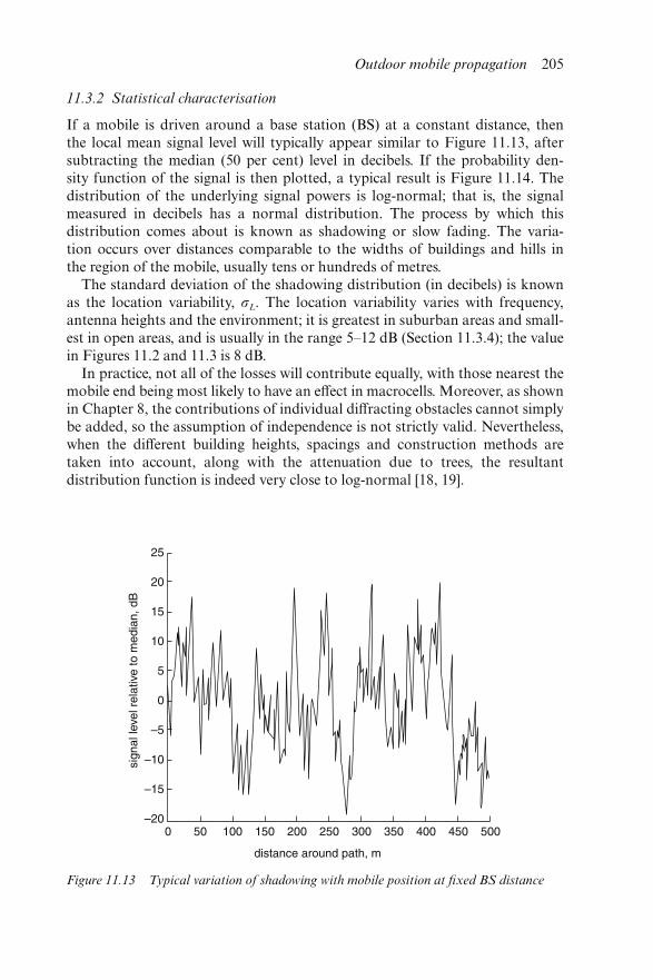
11.3.2 Statistical characterisation
If a mobile is driven around a base station (BS) at a constant distance, thenthe local mean signal level will typically appear similar to Figure 11.13, aftersubtracting the median (50 per cent) level in decibels. If the probability den-sity function of the signal is then plotted, a typical result is Figure 11.14. Thedistribution of the underlying signal powers is log-normal; that is, the signalmeasured in decibels has a normal distribution. The process by which thisdistribution comes about is known as shadowing or slow fading. The varia-tion occurs over distances comparable to the widths of buildings and hills inthe region of the mobile, usually tens or hundreds of metres.
The standard deviation of the shadowing distribution (in decibels) is knownas the location variability, σL. The location variability varies with frequency,antenna heights and the environment; it is greatest in suburban areas and small-est in open areas, and is usually in the range 5–12 dB (Section 11.3.4); the valuein Figures 11.2 and 11.3 is 8 dB.
In practice, not all of the losses will contribute equally, with those nearest themobile end being most likely to have an effect in macrocells. Moreover, as shownin Chapter 8, the contributions of individual diffracting obstacles cannot simplybe added, so the assumption of independence is not strictly valid. Nevertheless,when the different building heights, spacings and construction methods aretaken into account, along with the attenuation due to trees, the resultantdistribution function is indeed very close to log-normal [18, 19].
Figure 11.13 Typical variation of shadowing with mobile position at fixed BS distance
Outdoor mobile propagation 205
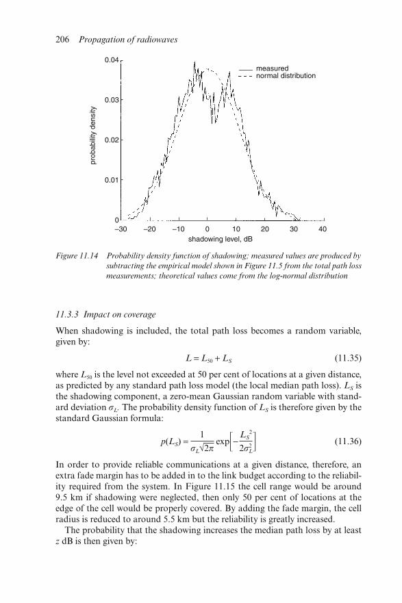
11.3.3 Impact on coverage
When shadowing is included, the total path loss becomes a random variable,given by:
L = L50 + LS (11.35)
where L50 is the level not exceeded at 50 per cent of locations at a given distance,as predicted by any standard path loss model (the local median path loss). LS isthe shadowing component, a zero-mean Gaussian random variable with stand-ard deviation σL. The probability density function of LS is therefore given by thestandard Gaussian formula:
p(LS) = 1
σL√2π exp− LS
2
2σ2L� (11.36)
In order to provide reliable communications at a given distance, therefore, anextra fade margin has to be added in to the link budget according to the reliabil-ity required from the system. In Figure 11.15 the cell range would be around9.5 km if shadowing were neglected, then only 50 per cent of locations at theedge of the cell would be properly covered. By adding the fade margin, the cellradius is reduced to around 5.5 km but the reliability is greatly increased.
The probability that the shadowing increases the median path loss by at leastz dB is then given by:
Figure 11.14 Probability density function of shadowing; measured values are produced by
subtracting the empirical model shown in Figure 11.5 from the total path loss
measurements; theoretical values come from the log-normal distribution
206 Propagation of radiowaves
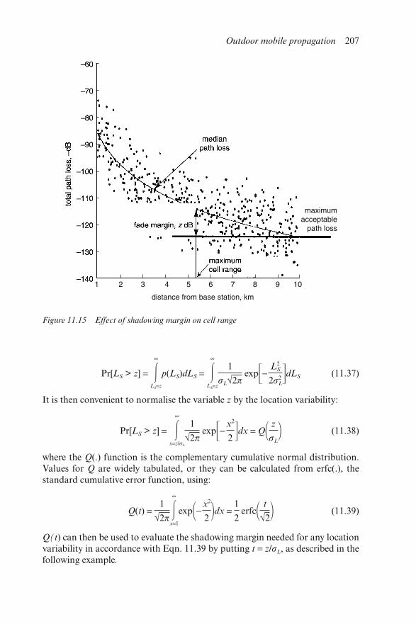
Pr[LS > z] = �∞
LS=z
p(LS)dLS = �∞
LS=z
1
σL√2πexp− L2
S
2σ2L�dLS (11.37)
It is then convenient to normalise the variable z by the location variability:
Pr[LS > z] = �∞
x=z/σL
1
√2π exp−x2
2 �dx = Q� z
σL� (11.38)
where the Q(.) function is the complementary cumulative normal distribution.Values for Q are widely tabulated, or they can be calculated from erfc(.), thestandard cumulative error function, using:
Q(t) = 1
√2π�∞
x=1
exp�−x2
2 �dx = 1
2 erfc� t
√2� (11.39)
Q(t) can then be used to evaluate the shadowing margin needed for any locationvariability in accordance with Eqn. 11.39 by putting t = z/σL, as described in thefollowing example.
Figure 11.15 Effect of shadowing margin on cell range
Outdoor mobile propagation 207
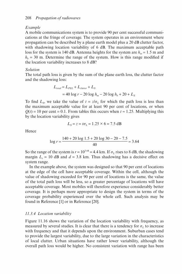
Example
A mobile communications system is to provide 90 per cent successful communi-cations at the fringe of coverage. The system operates in an environment wherepropagation can be described by a plane earth model plus a 20 dB clutter factor,with shadowing location variability of 6 dB. The maximum acceptable pathloss for the system is 140 dB. Antenna heights for the system are hm = 1.5 m andhb = 30 m. Determine the range of the system. How is this range modified ifthe location variability increases to 8 dB?
Solution
The total path loss is given by the sum of the plane earth loss, the clutter factorand the shadowing loss:
Ltotal = LPEL + Lclutter + LS
= 40 log r − 20 log hm − 20 log hb + 20 + LS
To find LS, we take the value of t = z/σL for which the path loss is less thanthe maximum acceptable value for at least 90 per cent of locations, or whenQ(t) = 10 per cent = 0.1. From tables this occurs when t ≈ 1.25. Multiplying thisby the location variability gives
LS = z = tσL = 1.25 × 6 = 7.5 dB
Hence
log r = 140 + 20 log 1.5 + 20 log 30 − 20 − 7.5
40 = 3.64
So the range of the system is r = 103.64 = 4.4 km. If σL rises to 8 dB, the shadowingmargin Ls = 10 dB and d = 3.8 km. Thus shadowing has a decisive effect onsystem range.
In the example above, the system was designed so that 90 per cent of locationsat the edge of the cell have acceptable coverage. Within the cell, although thevalue of shadowing exceeded for 90 per cent of locations is the same, the valueof the total path loss will be less, so a greater percentage of locations will haveacceptable coverage. Most mobiles will therefore experience considerably bettercoverage. It is perhaps more appropriate to design the system in terms of thecoverage probability experienced over the whole cell. Such analysis may befound in Reference [1] or in Reference [20].
11.3.4 Location variability
Figure 11.16 shows the variation of the location variability with frequency, asmeasured by several studies. It is clear that there is a tendency for σL to increasewith frequency and that it depends upon the environment. Suburban cases tendto provide the largest variability, due to the large variation in the characteristicsof local clutter. Urban situations have rather lower variability, although theoverall path loss would be higher. No consistent variation with range has been
208 Propagation of radiowaves
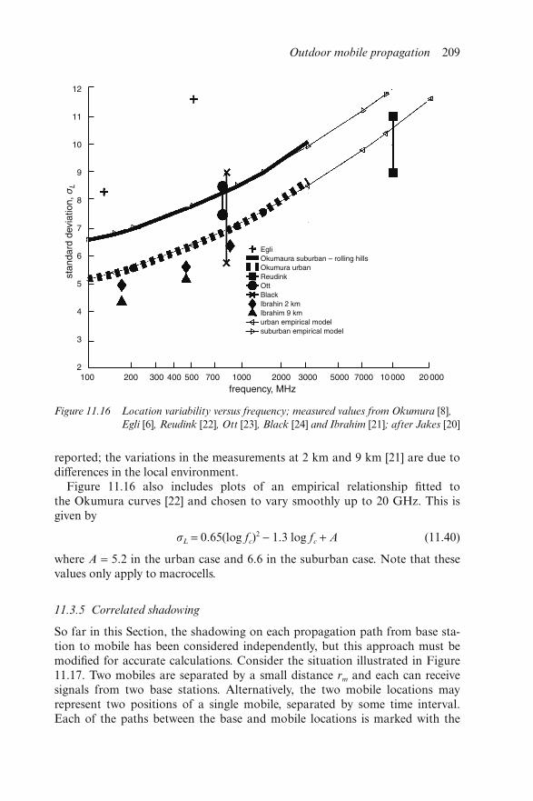
reported; the variations in the measurements at 2 km and 9 km [21] are due todifferences in the local environment.
Figure 11.16 also includes plots of an empirical relationship fitted tothe Okumura curves [22] and chosen to vary smoothly up to 20 GHz. This isgiven by
σL = 0.65(log fc)2 − 1.3 log fc + A (11.40)
where A = 5.2 in the urban case and 6.6 in the suburban case. Note that thesevalues only apply to macrocells.
11.3.5 Correlated shadowing
So far in this Section, the shadowing on each propagation path from base sta-tion to mobile has been considered independently, but this approach must bemodified for accurate calculations. Consider the situation illustrated in Figure11.17. Two mobiles are separated by a small distance rm and each can receivesignals from two base stations. Alternatively, the two mobile locations mayrepresent two positions of a single mobile, separated by some time interval.Each of the paths between the base and mobile locations is marked with the
Figure 11.16 Location variability versus frequency; measured values from Okumura [8],Egli [6], Reudink [22], Ott [23], Black [24] and Ibrahim [21]; after Jakes [20]
Outdoor mobile propagation 209
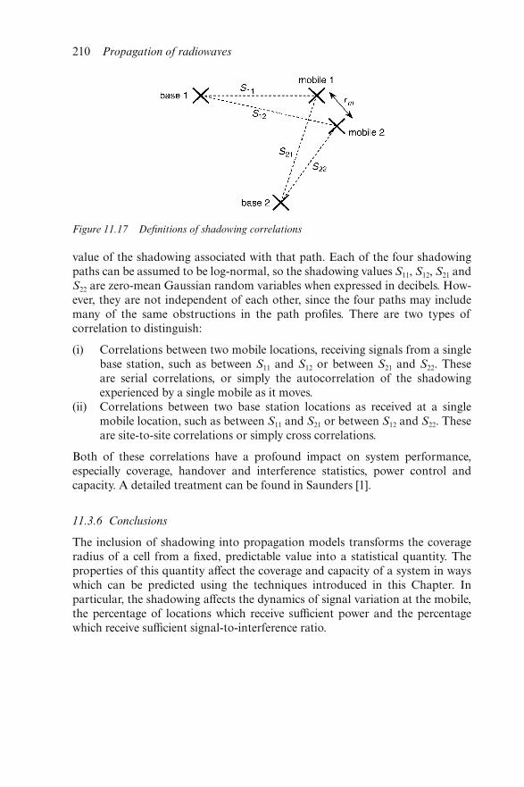
value of the shadowing associated with that path. Each of the four shadowingpaths can be assumed to be log-normal, so the shadowing values S11, S12, S21 andS22 are zero-mean Gaussian random variables when expressed in decibels. How-ever, they are not independent of each other, since the four paths may includemany of the same obstructions in the path profiles. There are two types ofcorrelation to distinguish:
(i) Correlations between two mobile locations, receiving signals from a singlebase station, such as between S11 and S12 or between S21 and S22. Theseare serial correlations, or simply the autocorrelation of the shadowingexperienced by a single mobile as it moves.
(ii) Correlations between two base station locations as received at a singlemobile location, such as between S11 and S21 or between S12 and S22. Theseare site-to-site correlations or simply cross correlations.
Both of these correlations have a profound impact on system performance,especially coverage, handover and interference statistics, power control andcapacity. A detailed treatment can be found in Saunders [1].
11.3.6 Conclusions
The inclusion of shadowing into propagation models transforms the coverageradius of a cell from a fixed, predictable value into a statistical quantity. Theproperties of this quantity affect the coverage and capacity of a system in wayswhich can be predicted using the techniques introduced in this Chapter. Inparticular, the shadowing affects the dynamics of signal variation at the mobile,the percentage of locations which receive sufficient power and the percentagewhich receive sufficient signal-to-interference ratio.
Figure 11.17 Definitions of shadowing correlations
210 Propagation of radiowaves
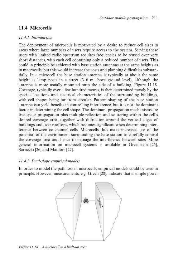
11.4 Microcells
11.4.1 Introduction
The deployment of microcells is motivated by a desire to reduce cell sizes inareas where large numbers of users require access to the system. Serving theseusers with limited radio spectrum requires frequencies to be reused over veryshort distances, with each cell containing only a reduced number of users. Thiscould in principle be achieved with base station antennas at the same heights asin macrocells, but this would increase the costs and planning difficulties substan-tially. In a microcell the base station antenna is typically at about the sameheight as lamp posts in a street (3–6 m above ground level), although theantenna is more usually mounted onto the side of a building, Figure 11.18.Coverage, typically over a few hundred metres, is then determined mostly by thespecific locations and electrical characteristics of the surrounding buildings,with cell shapes being far from circular. Pattern shaping of the base stationantenna can yield benefits in controlling interference, but it is not the dominantfactor in determining the cell shape. The dominant propagation mechanisms arefree-space propagation plus multiple reflection and scattering within the cell’sdesired coverage area, together with diffraction around the vertical edges ofbuildings and over rooftops, which becomes significant when determining inter-ference between co-channel cells. Microcells thus make increased use of thepotential of the environment surrounding the base station to carefully controlthe coverage area and hence to manage the interference between sites. Moregeneral information on microcell systems is available in Greenstein [25],Sarnecki [26] and Madfors [27].
11.4.2 Dual-slope empirical models
In order to model the path loss in microcells, empirical models could be used inprinciple. However, measurements, e.g. Green [28], indicate that a simple power
Figure 11.18 A microcell in a built-up area
Outdoor mobile propagation 211
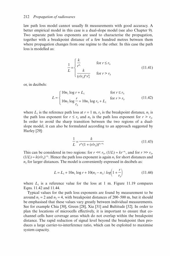
law path loss model cannot usually fit measurements with good accuracy. Abetter empirical model in this case is a dual-slope model (see also Chapter 9).Two separate path loss exponents are used to characterise the propagation,together with a breakpoint distance of a few hundred metres between themwhere propagation changes from one regime to the other. In this case the pathloss is modelled as:
1
L=
k
rn1for r ≤ rb
(11.41)k
(r/rb)n2rn1
b
for r > rb
⎧⎭⎫⎩
or, in decibels:
L =10n1 log r + L1
10n2 logr
rb
+ 10n1 log rb + L1
for r ≤ rb
for r > rb(11.42)
⎧⎨⎩
where L1 is the reference path loss at r = 1 m, rb is the breakpoint distance, n1 isthe path loss exponent for r ≤ rb and n2 is the path loss exponent for r > rb.In order to avoid the sharp transition between the two regions of a dual-slope model, it can also be formulated according to an approach suggested byHarley [29]:
1
L =
k
rn1(1 + (r/rb))n2−n1
(11.43)
This can be considered in two regions: for r << rb, (1/L) ≈ kr−n1, and for r >> rb,(1/L) ≈ k(r/rb)
−n2. Hence the path loss exponent is again n1 for short distances andn2 for larger distances. The model is conveniently expressed in decibels as:
L = L1 + 10n1 log r + 10(n2 − n1) log�1 + r
rb� (11.44)
where L1 is a reference value for the loss at 1 m. Figure 11.19 comparesEqns. 11.42 and 11.44.
Typical values for the path loss exponents are found by measurement to bearound n1 = 2 and n2 = 4, with breakpoint distances of 200–500 m, but it shouldbe emphasised that these values vary greatly between individual measurements.See for example Chia [30], Green [28], Xia [31] and Bultitude [32]. In order toplan the locations of microcells effectively, it is important to ensure that co-channel cells have coverage areas which do not overlap within the breakpointdistance. The rapid reduction of signal level beyond the breakpoint then pro-duces a large carrier-to-interference ratio, which can be exploited to maximisesystem capacity.
212 Propagation of radiowaves
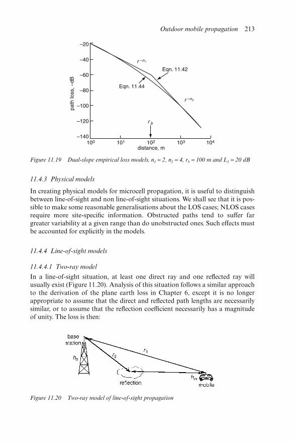
11.4.3 Physical models
In creating physical models for microcell propagation, it is useful to distinguishbetween line-of-sight and non line-of-sight situations. We shall see that it is pos-sible to make some reasonable generalisations about the LOS cases; NLOS casesrequire more site-specific information. Obstructed paths tend to suffer fargreater variability at a given range than do unobstructed ones. Such effects mustbe accounted for explicitly in the models.
11.4.4 Line-of-sight models
11.4.4.1 Two-ray model
In a line-of-sight situation, at least one direct ray and one reflected ray willusually exist (Figure 11.20). Analysis of this situation follows a similar approachto the derivation of the plane earth loss in Chapter 6, except it is no longerappropriate to assume that the direct and reflected path lengths are necessarilysimilar, or to assume that the reflection coefficient necessarily has a magnitudeof unity. The loss is then:
Figure 11.19 Dual-slope empirical loss models, n1 = 2, n2 = 4, rb = 100 m and L1 = 20 dB
Figure 11.20 Two-ray model of line-of-sight propagation
Outdoor mobile propagation 213
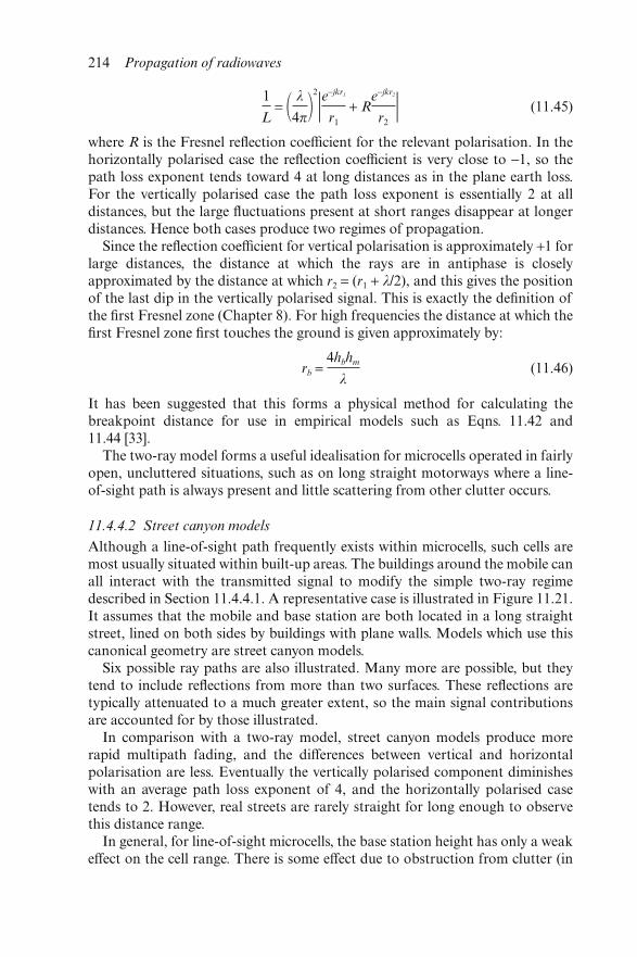
1
L = � λ
4π�2
�e−jkr1
r1
+ Re−jkr2
r2� (11.45)
where R is the Fresnel reflection coefficient for the relevant polarisation. In thehorizontally polarised case the reflection coefficient is very close to −1, so thepath loss exponent tends toward 4 at long distances as in the plane earth loss.For the vertically polarised case the path loss exponent is essentially 2 at alldistances, but the large fluctuations present at short ranges disappear at longerdistances. Hence both cases produce two regimes of propagation.
Since the reflection coefficient for vertical polarisation is approximately +1 forlarge distances, the distance at which the rays are in antiphase is closelyapproximated by the distance at which r2 = (r1 + λ/2), and this gives the positionof the last dip in the vertically polarised signal. This is exactly the definition ofthe first Fresnel zone (Chapter 8). For high frequencies the distance at which thefirst Fresnel zone first touches the ground is given approximately by:
rb = 4hbhm
λ(11.46)
It has been suggested that this forms a physical method for calculating thebreakpoint distance for use in empirical models such as Eqns. 11.42 and11.44 [33].
The two-ray model forms a useful idealisation for microcells operated in fairlyopen, uncluttered situations, such as on long straight motorways where a line-of-sight path is always present and little scattering from other clutter occurs.
11.4.4.2 Street canyon models
Although a line-of-sight path frequently exists within microcells, such cells aremost usually situated within built-up areas. The buildings around the mobile canall interact with the transmitted signal to modify the simple two-ray regimedescribed in Section 11.4.4.1. A representative case is illustrated in Figure 11.21.It assumes that the mobile and base station are both located in a long straightstreet, lined on both sides by buildings with plane walls. Models which use thiscanonical geometry are street canyon models.
Six possible ray paths are also illustrated. Many more are possible, but theytend to include reflections from more than two surfaces. These reflections aretypically attenuated to a much greater extent, so the main signal contributionsare accounted for by those illustrated.
In comparison with a two-ray model, street canyon models produce morerapid multipath fading, and the differences between vertical and horizontalpolarisation are less. Eventually the vertically polarised component diminisheswith an average path loss exponent of 4, and the horizontally polarised casetends to 2. However, real streets are rarely straight for long enough to observethis distance range.
In general, for line-of-sight microcells, the base station height has only a weakeffect on the cell range. There is some effect due to obstruction from clutter (in
214 Propagation of radiowaves
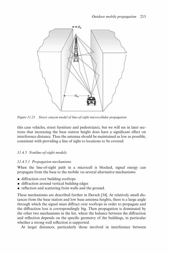
this case vehicles, street furniture and pedestrians), but we will see in later sec-tions that increasing the base station height does have a significant effect oninterference distance. Thus the antenna should be maintained as low as possible,consistent with providing a line of sight to locations to be covered.
11.4.5 Nonline-of-sight models
11.4.5.1 Propagation mechanisms
When the line-of-sight path in a microcell is blocked, signal energy canpropagate from the base to the mobile via several alternative mechanisms:
• diffraction over building rooftops
• diffraction around vertical building edges
• reflection and scattering from walls and the ground.
These mechanisms are described further in Dersch [34]. At relatively small dis-tances from the base station and low base antenna heights, there is a large anglethrough which the signal must diffract over rooftops in order to propagate andthe diffraction loss is correspondingly big. Then propagation is dominated bythe other two mechanisms in the list, where the balance between the diffractionand reflection depends on the specific geometry of the buildings, in particularwhether a strong wall reflection is supported.
At larger distances, particularly those involved in interference between
Figure 11.21 Street canyon model of line-of-sight microcellular propagation
Outdoor mobile propagation 215
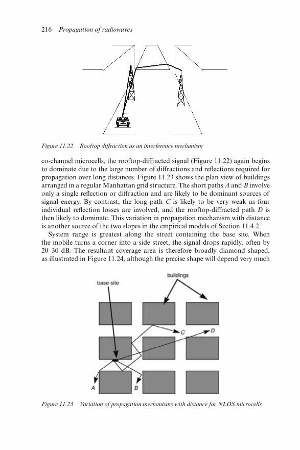
co-channel microcells, the rooftop-diffracted signal (Figure 11.22) again beginsto dominate due to the large number of diffractions and reflections required forpropagation over long distances. Figure 11.23 shows the plan view of buildingsarranged in a regular Manhattan grid structure. The short paths A and B involveonly a single reflection or diffraction and are likely to be dominant sources ofsignal energy. By contrast, the long path C is likely to be very weak as fourindividual reflection losses are involved, and the rooftop-diffracted path D isthen likely to dominate. This variation in propagation mechanism with distanceis another source of the two slopes in the empirical models of Section 11.4.2.
System range is greatest along the street containing the base site. Whenthe mobile turns a corner into a side street, the signal drops rapidly, often by20–30 dB. The resultant coverage area is therefore broadly diamond shaped,as illustrated in Figure 11.24, although the precise shape will depend very much
Figure 11.22 Rooftop diffraction as an interference mechanism
Figure 11.23 Variation of propagation mechanisms with distance for NLOS microcells
216 Propagation of radiowaves
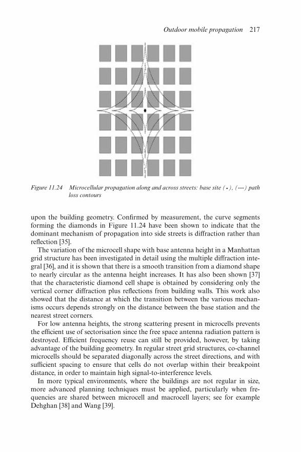
upon the building geometry. Confirmed by measurement, the curve segmentsforming the diamonds in Figure 11.24 have been shown to indicate that thedominant mechanism of propagation into side streets is diffraction rather thanreflection [35].
The variation of the microcell shape with base antenna height in a Manhattangrid structure has been investigated in detail using the multiple diffraction inte-gral [36], and it is shown that there is a smooth transition from a diamond shapeto nearly circular as the antenna height increases. It has also been shown [37]that the characteristic diamond cell shape is obtained by considering only thevertical corner diffraction plus reflections from building walls. This work alsoshowed that the distance at which the transition between the various mechan-isms occurs depends strongly on the distance between the base station and thenearest street corners.
For low antenna heights, the strong scattering present in microcells preventsthe efficient use of sectorisation since the free space antenna radiation pattern isdestroyed. Efficient frequency reuse can still be provided, however, by takingadvantage of the building geometry. In regular street grid structures, co-channelmicrocells should be separated diagonally across the street directions, and withsufficient spacing to ensure that cells do not overlap within their breakpointdistance, in order to maintain high signal-to-interference levels.
In more typical environments, where the buildings are not regular in size,more advanced planning techniques must be applied, particularly when fre-quencies are shared between microcell and macrocell layers; see for exampleDehghan [38] and Wang [39].
Figure 11.24 Microcellular propagation along and across streets: base site (⋅), (---) path
loss contours
Outdoor mobile propagation 217
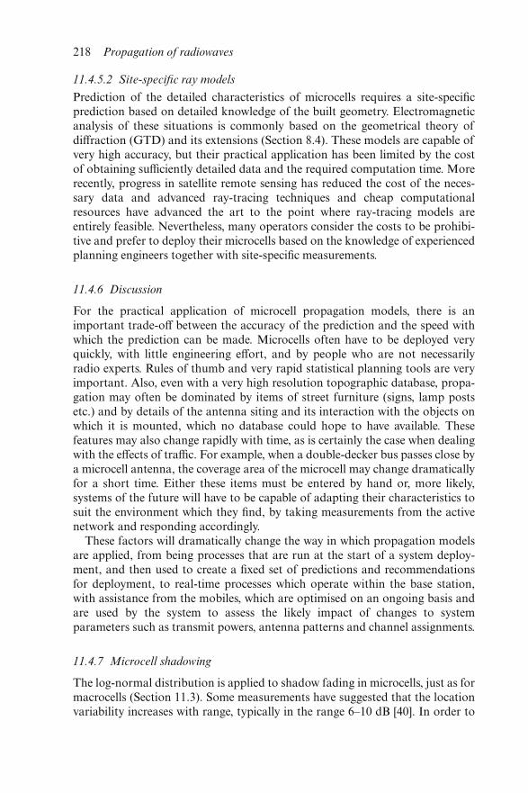
11.4.5.2 Site-specific ray models
Prediction of the detailed characteristics of microcells requires a site-specificprediction based on detailed knowledge of the built geometry. Electromagneticanalysis of these situations is commonly based on the geometrical theory ofdiffraction (GTD) and its extensions (Section 8.4). These models are capable ofvery high accuracy, but their practical application has been limited by the costof obtaining sufficiently detailed data and the required computation time. Morerecently, progress in satellite remote sensing has reduced the cost of the neces-sary data and advanced ray-tracing techniques and cheap computationalresources have advanced the art to the point where ray-tracing models areentirely feasible. Nevertheless, many operators consider the costs to be prohibi-tive and prefer to deploy their microcells based on the knowledge of experiencedplanning engineers together with site-specific measurements.
11.4.6 Discussion
For the practical application of microcell propagation models, there is animportant trade-off between the accuracy of the prediction and the speed withwhich the prediction can be made. Microcells often have to be deployed veryquickly, with little engineering effort, and by people who are not necessarilyradio experts. Rules of thumb and very rapid statistical planning tools are veryimportant. Also, even with a very high resolution topographic database, propa-gation may often be dominated by items of street furniture (signs, lamp postsetc.) and by details of the antenna siting and its interaction with the objects onwhich it is mounted, which no database could hope to have available. Thesefeatures may also change rapidly with time, as is certainly the case when dealingwith the effects of traffic. For example, when a double-decker bus passes close bya microcell antenna, the coverage area of the microcell may change dramaticallyfor a short time. Either these items must be entered by hand or, more likely,systems of the future will have to be capable of adapting their characteristics tosuit the environment which they find, by taking measurements from the activenetwork and responding accordingly.
These factors will dramatically change the way in which propagation modelsare applied, from being processes that are run at the start of a system deploy-ment, and then used to create a fixed set of predictions and recommendationsfor deployment, to real-time processes which operate within the base station,with assistance from the mobiles, which are optimised on an ongoing basis andare used by the system to assess the likely impact of changes to systemparameters such as transmit powers, antenna patterns and channel assignments.
11.4.7 Microcell shadowing
The log-normal distribution is applied to shadow fading in microcells, just as formacrocells (Section 11.3). Some measurements have suggested that the locationvariability increases with range, typically in the range 6–10 dB [40]. In order to
218 Propagation of radiowaves
account for microcell shadowing cross correlation, the shadowing can be separ-ated into two parts, one of which is caused by obstructions very local to themobile and is therefore common to all paths, and another which is specific to thetransport of energy from the mobile to a particular base station [41].
11.4.8 Conclusions
Propagation in microcells can be modelled using either empirical or physicalmodels, just like the macrocells in section 11.2. In either case, however, theclutter surrounding the base station has a significant impact on the cell shapeand this must be accounted for to avoid serious prediction errors. In particular, asimple path loss exponent model is inadequate and dual-slope behaviour mustbe accounted for. This clutter also creates difficulties in deploying antennas,since the clutter disrupts the free-space antenna radiation pattern. Nevertheless,the enormous potential offered by microcells in creating high-capacity cellularsystems makes them increasingly attractive methods of providing outdoorcoverage in areas with high user densities [38].
11.5 References
1 SAUNDERS, S.R.: ‘Antennas and propagation for wireless communicationsystems’ (John Wiley, Chichester, 1999)
2 SHANNON, C.: ‘A mathematical theory of communication’, Bell Syst.Tech. J., 1948, 27, 379–423 and 623–56. Reprinted in SLOANE, N.J.A. andWYNER, A.D.: ‘Claude Elwood Shannon: collected papers’ (IEEE Press,New York, 1993)
3 CLARKE, R.H.: ‘A statistical theory of mobile radio reception’, Bell Syst.Tech. J., 1968, 47, (6), pp.957–1000
4 PARSONS, J. D. ‘The mobile radio propagation channel’ (John Wiley,Chichester, 1992)
5 LEE, W.C.Y.: ‘Estimate of local average power of a mobile radio signal’,IEEE Trans. Veh. Tech., 1985, 34 (1), pp.22–27
6 EGLI, J.J, ‘Radio propagation above 40 MC over irregular terrain’, Proc.IRE, 1957, pp.1383–91
7 DELISLE, G.Y, LEFEVRE, J., LECOURS, M., and CHOUINARD, J.:‘Propagation loss prediction: a comparative study with application to themobile radio channel’, IEEE Trans. Veh. Tech., 1985, 26, (4), pp.295–308
8 OKUMURA, Y., OHMORI, E., KAWANO, T. and FUKUDA, K.: ‘Fieldstrength and its variability in VHF and UHF land mobile radio service’,Rev. Electr. Commun. Lab., 1968, 16, pp.825–73
9 HATA, M.: ‘Empirical formula for propagation loss in land mobile radioservices’, IEEE Trans. Veh. Tech., 1980, 29, pp.317–25
10 International Telecommunication Union: ‘Recommendation ITU-RP.529-2: Prediction methods for the terrestrial land mobile service in theVHF and UHF bands’, Geneva, 1997
11 Final report of the COST-207 management committee: ‘Digital land mobile
Outdoor mobile propagation 219
radio communications’ Commission of the European Communities,L-2920, Luxembourg, 1989
12 KOZONO, S. and WATANABE, K.: ‘Influence of environmental buildingson UHF land mobile radio propagation’, IEEE Trans. Commun., 1977, 25,(10), pp.1133–43
13 COST 231 final report: ‘Digital mobile radio: COST 231 view on the evolu-tion towards 3rd generation systems’, Commission of the EuropeanCommunities and COST Telecommunications, Brussels, 1999
14 IKEGAMI, F., TAKEUCHI, T., and YOSHIDA, S.: ‘Theoretical predic-tion of mean field strength for urban mobile radio’, IEEE Trans. AntennasPropag., 39, (3), pp.299–302
15 SAUNDERS, S.R., and BONAR, F.R.: ‘Prediction of mobile radio wavepropagation over buildings of irregular heights and spacings’, IEEE Trans.Antennas Propag., 1994, 42, (2), pp.137–44
16 SAUNDERS, S.R., and BONAR, F.R.: ‘Explicit multiple building diffrac-tion attenuation function for mobile radio wave propagation’, Electron.Lett., 1991, 27 (14), pp.1276–77
17 WALFISCH, J., and BERTONI, H.L.: ‘A theoretical model of UHFpropagation in urban environments, IEEE Trans. Antennas. Propag., 1988,36, (12), pp. 1788–96
18 CHRYSANTHOU, C., and BERTONI, H.L.: ‘Variability of sector aver-aged signals for UHF propagation in cities’, IEEE Trans. Veh. Tech., 1990,39 (4), pp.352–58
19 SAUNDERS, S.R., and BONAR, F.R.: ‘Mobile radio propagation in built-up areas: a numerical model of slow fading’, Proc. 41st IEEE VehicularTechnology Society Conference, 1991, pp.295–300
20 JAKES, W.C.: ‘Microwave mobile communications’, (IEEE, New York,1994)
21 IBRAHIM, M.F., and PARSONS, J.D.: ‘Signal strength prediction inbuilt-up areas’, IEE Proc. F, 1983, 130, (5), pp.377–84
22 REUDINK, D.O.: ‘Comparison of radio transmission at X-band frequen-cies in suburban and urban areas’, IEEE Trans. Antennas Propag., 1972, 20,p.470
23 OTT, G.D.: ‘Data processing summary and path loss statistics for Philadel-phia HCNTS measurements program’. Quoted in JAKES [20]
24 BLACK, D.M., and REUDINK, D.O.: ‘Some characteristics of mobileradio propagation at 836 MHz in the Philadelphia area’, IEEE Trans. Veh.Tech., 1972, 21 (2), pp.45–51
25 GREENSTEIN, L.J., ARMITAY, N., CHU, T.S. et al.: ‘Microcells inpersonal communication systems’, IEEE Commun. Mag., 1992, 30, (12),pp.76–88
26 SARNECKI, J., VINODRAI, C., JAVED, A., O’KELLY, P. and DICK,K.: ‘Microcell design principles’, IEEE Commun. Mag, 1993, 31, (4),pp.76–82
27 MADFORS, M., WALLSTEDT, K., et al.: ‘High capacity with limitedspectrum in cellular systems’, IEEE Commun. Mag., 1997, 35, (8), pp.38–46
28 GREEN, E.: ‘Radio link design for microcellular systems’, BT Tech. J,1990, 8, (1), pp.85–96
29 HARLEY, P.: ‘Short distance attenuation measurements at 900 MHz and
220 Propagation of radiowaves
1.8 GHz using low antenna heights for microcells’, IEEE J. Sel. AreasCommun., 1989, 7, (1), pp.5–11
30 CHIA, S.T.S.: ‘Radiowave propagation and handover criteria for micro-cells’, BT Tech. J., 1990, 8, (4), pp.50–61
31 XIA, H.H., BERTONI, H.L., MACIEL, L.R., LINDSAY-STEWART, A.and ROWE, R.: ‘Microcellular propagation characteristics for personalcommunications in urban and suburban environments’, IEEE Trans. Veh.Tech., 1994, 43, (3), pp.743–752
32 BULTITUDE, R.J.C., and HUGHES. D.A.: ‘Propagation loss at 1.8 GHzon microcellular mobile radio channels’. Proc. IEEE international sym-posium on Personal, indoor and mobile radio communications, (PIMRC ’96),October 1996, pp.786–90
33 XIA, H.H., BERTONI, H.L., MACIEL, L.R., LINDSAY-STEWART, A.,and ROWE, R.: ‘Radio propagation characteristics for line-of-sight micro-cellular and personal communications’, IEEE Trans. Antennas Propag.,1993, 41, (10), pp.1439–1447
34 DERSCH, U., and ZOLLINGER, E.: ‘Propagation mechanisms in micro-cell and indoor environments’ IEEE Trans. Veh. Tech, 1994, 43, (4),pp.1058–66
35 GOLDSMITH, A.J., and GOLDSMITH, L.J.: ‘A measurement-basedmodel for predicting coverage areas of urban microcells’, IEEE J. Sel. AreasCommun., 1993, 11, (7), pp.1013–23
36 MACIEL, L.R., and BERTONI, H.L.: ‘Cell shape for microcellular sys-tems in residential and commercial environments’, IEEE Trans. Veh. Tech.,1994, 43, (2), pp.270–278
37 ERCEG, V., RUSTAKO, A.J., and ROMAN, P.S.: ‘Diffraction around cor-ners and its effects on the microcell coverage area in urban and suburbanenvironments at 900 MHz, 2 GHz, and 6 GHz’, IEEE Trans. Veh. Tech.,1994, 43, (3), pp.762–66
38 DEHGHAN, S., and STEELE, R.: ‘Small cell city’, IEEE Commun. Mag.,1997, 35, (8), pp.52–59
39 WANG, L.C., STUBEA, G.L., and LEA, C.T.: ‘Architecture design,frequency planning, and performance analysis for a microcell/macrocelloverlaying system’, IEEE Trans. Veh. Tech., 1997, 46, (4), pp.836–48
40 FEUERSTEIN, M.J., BLACKARD, K.L., RAPPAPORT, T.S., and SEI-DEL, S.Y.: ‘Path loss, delay spread and outage models as functions ofantenna height for microcellular system design’, IEEE Trans. Veh. Tech.,1994, 43, (3), pp.487–98
41 ARNOLD, H.W., COX, D.C., and MURRAY, R.R.: ‘Macroscopic diver-sity performance measured in the 800 MHz portable radio communicationsenvironment’, IEEE Trans. Antennas Propag., 1988, 36, (2), pp.277–80
Outdoor mobile propagation 221

Chapter 12
Propagation in rain and clouds
J.W.F. Goddard
12.1 Introduction
Water appears in the atmosphere in a variety of forms, usually referred to by theterm hydrometeor, which includes particles as diverse as cloud, rain drops,snowflakes, ice crystals, hail and graupel. Of these, rain, hail, graupel and snoware generally recognised as precipitation. The effects that hydrometeors have oncommunications systems are dependent both on the system frequency and thetype of particle present. At any given instant, of course, more than one type ofparticle will affect a given link. For example, an earth–space link may oftenencounter rain over the lower part of the path, and snow at greater heights.
We will consider first the various forms of hydrometeor, together with theirrelevance to radiowave propagation. A brief theoretical framework will thenbe presented as a background to the model development process and, finally,specific effects of hydrometeors on systems will be considered.
12.2 Rain
12.2.1 Rain drop size distributions
In modelling the effects of rain on radiowaves propagating through it, or scat-tered from it, the usual problem is to numerically relate two physically distinctquantities. For example, we might wish to relate a microwave-specific attenuationto a rain rate or to a radar reflectivity, a rain rate to a reflectivity, or a differentialattenuation between two polarisations to an absolute attenuation in one etc. Allthese quantities are obtained as integrals over the drop size distribution functionN(D), defined such that N(D)dD is the number of drops per cubic metre withdrop diameters D between D and D + dD. (As all but the smallest drops arenonspherical, D is usually defined as being that of an equivolumic sphere.)
Nearly always the contributions to the two quantities to be related have a differ-ent diameter dependence, and some assumptions about the shape of the func-tion N(D) must be made.
Satisfactory results are generally obtained by using an ideal mathematicalform for N(D), described by a small number of free parameters. Large depar-tures from the ideal forms undoubtedly occur in real rain, but the situation iseased by the fact that relationships between quantities are in practice often onlyrequired to hold on a mean statistical basis. Also, fine structure in N(D) tends todisappear in the integration.
Much modelling to date has used an exponential form for N(D):
N(D) = N0exp(−ΛD) (12.1)
Early work [1] indicated that Λ tends to increase with rain rate R, and that thesedistributions can be reduced to a one-parameter family by treating the relationas deterministic, with:
Λ = 4.1 R−0.21 (12.2)
where Λ is in mm−1 and R is in mm h−1.Once Λ is determined from R, so is N0 by the requirement that the integral of
N(D)D3 V(D), where V is the drop terminal velocity, actually gives R. Typicalvalues of N0 were found to be around 8000 mm−1 m−3, with this form of distribu-tion becoming known as the Marshall–Palmer distribution. The parameter, Λ,can be shown to be related to the median volume drop diameter of the distribu-tion, D0, through the relation:
Λ = 3.67 / D0 (12.3)
The Laws–Parsons distribution [2], which predates the Marshall–Palmerapproach and is also much used, is an empirically measured form for N(D)which is tabulated numerically rather than expressed mathematically. It is similarto the Marshall–Palmer form except that it has slightly fewer small drops.
Subsequent work which followed the development of disdrometers, instru-ments capable of automatically recording the size distribution of drops, showedthat N0 could, in fact, vary quite considerably, both from one event to anotherand even within a rain event. In addition, the shape of the distribution was alsofound to vary significantly, which led to a more general form of distribution, thegamma-type distribution, being proposed [3]:
N(D) = N0Dme−(3.67+m)D/D0 (12.4)
Positive values of m reduce the numbers of drops at both the large and smallends of the size spectrum, compared with the exponential distribution obtainedwhen m = 0. In contrast, negative values of m increase the numbers of dropsat each end of the spectrum. Figure 12.1 shows this effect for three differentdistributions, all with the same rainfall rate (5 mm h−1) and the same D0 (1 mm).
It is interesting to note from Figure 12.1 that the three distributions have verydifferent numbers of small and large drops, but the same integrated rainfall rate.
224 Propagation of radiowaves
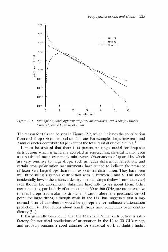
The reason for this can be seen in Figure 12.2, which indicates the contributionfrom each drop size to the total rainfall rate. For example, drops between 1 and2 mm diameter contribute 60 per cent of the total rainfall rate of 5 mm h−1.
It must be stressed that there is at present no single model for drop-sizedistributions which is generally accepted as representing physical reality, evenas a statistical mean over many rain events. Observations of quantities whichare very sensitive to large drops, such as radar differential reflectivity, andcertain cross-polarisation measurements, have tended to indicate the presenceof fewer very large drops than in an exponential distribution. They have beenwell fitted using a gamma distribution with m between 3 and 5. This modelincidentally lowers the assumed density of small drops (below 1 mm diameter)even though the experimental data may have little to say about them. Othermeasurements, particularly of attenuation at 30 to 300 GHz, are more sensitiveto small drops and make no strong implication about the presumed cut-offpoint for large drops, although work in the UK has suggested that a log-normal form of distribution would be appropriate for millimetric attenuationprediction [4]. Deductions about small drops have sometimes been contra-dictory [3,4].
It has generally been found that the Marshall–Palmer distribution is satis-factory for statistical predictions of attenuation in the 10 to 30 GHz range,and probably remains a good estimate for statistical work at slightly higher
Figure 12.1 Examples of three different drop-size distributions, with a rainfall rate of
5 mm h−1, and a D0 value of 1 mm
Propagation in rain and clouds 225
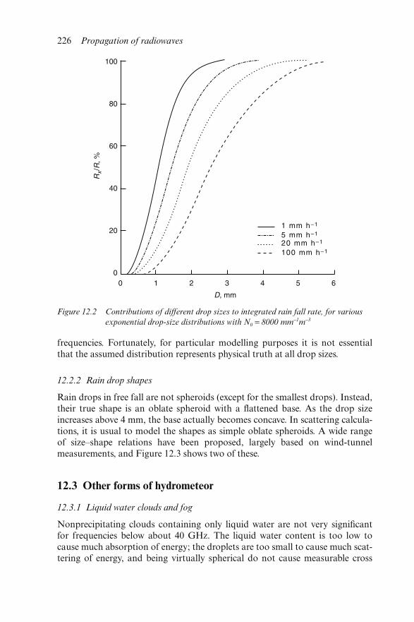
frequencies. Fortunately, for particular modelling purposes it is not essentialthat the assumed distribution represents physical truth at all drop sizes.
12.2.2 Rain drop shapes
Rain drops in free fall are not spheroids (except for the smallest drops). Instead,their true shape is an oblate spheroid with a flattened base. As the drop sizeincreases above 4 mm, the base actually becomes concave. In scattering calcula-tions, it is usual to model the shapes as simple oblate spheroids. A wide rangeof size–shape relations have been proposed, largely based on wind-tunnelmeasurements, and Figure 12.3 shows two of these.
12.3 Other forms of hydrometeor
12.3.1 Liquid water clouds and fog
Nonprecipitating clouds containing only liquid water are not very significantfor frequencies below about 40 GHz. The liquid water content is too low tocause much absorption of energy; the droplets are too small to cause much scat-tering of energy, and being virtually spherical do not cause measurable cross
Figure 12.2 Contributions of different drop sizes to integrated rain fall rate, for various
exponential drop-size distributions with N0 = 8000 mm−1m−3
226 Propagation of radiowaves
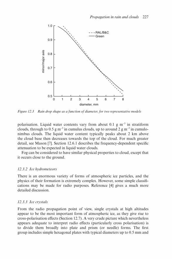
polarisation. Liquid water contents vary from about 0.1 g m−3 in stratiformclouds, through to 0.5 g m−3 in cumulus clouds, up to around 2 g m−3 in cumulo-nimbus clouds. The liquid water content typically peaks about 2 km abovethe cloud base then decreases towards the top of the cloud. For much greaterdetail, see Mason [7]. Section 12.6.1 describes the frequency-dependent specificattenuation to be expected in liquid water clouds.
Fog can be considered to have similar physical properties to cloud, except thatit occurs close to the ground.
12.3.2 Ice hydrometeors
There is an enormous variety of forms of atmospheric ice particles, and thephysics of their formation is extremely complex. However, some simple classifi-cations may be made for radio purposes. Reference [4] gives a much moredetailed discussion.
12.3.3 Ice crystals
From the radio propagation point of view, single crystals at high altitudesappear to be the most important form of atmospheric ice, as they give rise tocross-polarisation effects (Section 12.7). A very crude picture which neverthelessappears adequate to interpret radio effects (particularly cross polarisation) isto divide them broadly into plate and prism (or needle) forms. The firstgroup includes simple hexagonal plates with typical diameters up to 0.5 mm and
Figure 12.3 Rain drop shape as a function of diameter, for two representative models
Propagation in rain and clouds 227
thicknesses of perhaps 1/10 of the diameter, and the classical dendritic formwith complex hexagonal symmetry. The latter may reach 5 mm in diameter, witha thickness of probably less than 0.05 mm. The second group includes a varietyof long thin shapes including both needles and hexagonal prisms; typical lengthsare around 0.5 mm, and the ratio of length to breadth ranges from one to five.For modelling radio scatter when the crystals are small compared with the wave-length, a start can be made by treating them as either very oblate or very prolatespheroids.
The type of crystal depends in a complex way on the temperature at which itformed, and hence on the height. In the range −8 ° to −27 °C, plate types aretypical, with dendrites dominant in the subrange −14 ° to −17 °C. Below −27 °Cprisms are formed. Both classes can form in the 0 ° to −8 °C range, but they areprobably less important for propagation, except where differential phase effectsare of concern.
12.3.4 Snow
Snow consists of aggregated ice crystals, with large flakes forming only at tem-peratures just below freezing when the crystal surfaces become particularlysticky. In stratiform rain most of the ice is present as large flakes down to a fewhundred metres above the melting level, and at greater heights single crystals aremainly present. Dry snow does not appear to be very important for propagationof radiowaves, at least below 30 GHz. This is partly because of its low densitystructure (generally around 0.1 g m−3), giving it a permittivity close to unity, and(for polarisation effects) partly because the flakes tend to tumble without apreferred orientation.
12.3.5 Hail and graupel
Particles of hail and graupel are mainly formed by the accretion of supercooledcloud droplets in convective storms. Hail particles have densities close to that ofwater, and are often of roughly spherical shape, although a wide variety ofshapes have been recorded. Graupel has a density intermediate between those ofhail and snow and is usually of conical shape. Although of a higher apparentpermittivity than snow, dry hail and graupel are only weakly attenuating below30 GHz and do not appear to be very important for wave propagation effects.However, when they begin to melt, they scatter like very large raindrops. Notice-able polarisation effects might be expected but these seem to be of littlesignificance on a statistical basis, at least in a climate such as that in the UK.
12.3.6 Melting layer
In stratiform rain, partially melted snowflakes exist within a height interval ofabout 500 m around the 0 °C isotherm, and this melting layer can produceintense radio scattering effects, due to a combination of factors. The melting
228 Propagation of radiowaves
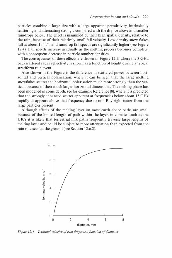
particles combine a large size with a large apparent permittivity, intrinsicallyscattering and attenuating strongly compared with the dry ice above and smallerraindrops below. The effect is magnified by their high spatial density, relative tothe rain, because of their relatively small fall velocity. Low density snow flakesfall at about 1 m s−1, and raindrop fall speeds are significantly higher (see Figure12.4). Fall speeds increase gradually as the melting process becomes complete,with a consequent decrease in particle number densities.
The consequences of these effects are shown in Figure 12.5, where the 3 GHzbackscattered radar reflectivity is shown as a function of height during a typicalstratiform rain event.
Also shown in the Figure is the difference in scattered power between hori-zontal and vertical polarisation, where it can be seen that the large meltingsnowflakes scatter the horizontal polarisation much more strongly than the ver-tical, because of their much larger horizontal dimensions. The melting phase hasbeen modelled in some depth, see for example Reference [8], where it is predictedthat the strongly enhanced scatter apparent at frequencies below about 15 GHzrapidly disappears above that frequency due to non-Rayleigh scatter from thelarge particles present.
Although effects of the melting layer on most earth–space paths are smallbecause of the limited length of path within the layer, in climates such as theUK’s it is likely that terrestrial link paths frequently traverse large lengths ofmelting layer and could be subject to more attenuation than expected from therain rate seen at the ground (see Section 12.6.2).
Figure 12.4 Terminal velocity of rain drops as a function of diameter
Propagation in rain and clouds 229
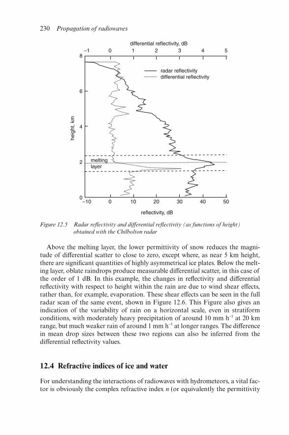
Above the melting layer, the lower permittivity of snow reduces the magni-tude of differential scatter to close to zero, except where, as near 5 km height,there are significant quantities of highly asymmetrical ice plates. Below the melt-ing layer, oblate raindrops produce measurable differential scatter, in this case ofthe order of 1 dB. In this example, the changes in reflectivity and differentialreflectivity with respect to height within the rain are due to wind shear effects,rather than, for example, evaporation. These shear effects can be seen in the fullradar scan of the same event, shown in Figure 12.6. This Figure also gives anindication of the variability of rain on a horizontal scale, even in stratiformconditions, with moderately heavy precipitation of around 10 mm h−1 at 20 kmrange, but much weaker rain of around 1 mm h−1 at longer ranges. The differencein mean drop sizes between these two regions can also be inferred from thedifferential reflectivity values.
12.4 Refractive indices of ice and water
For understanding the interactions of radiowaves with hydrometeors, a vital fac-tor is obviously the complex refractive index n (or equivalently the permittivity
Figure 12.5 Radar reflectivity and differential reflectivity (as functions of height)
obtained with the Chilbolton radar
230 Propagation of radiowaves
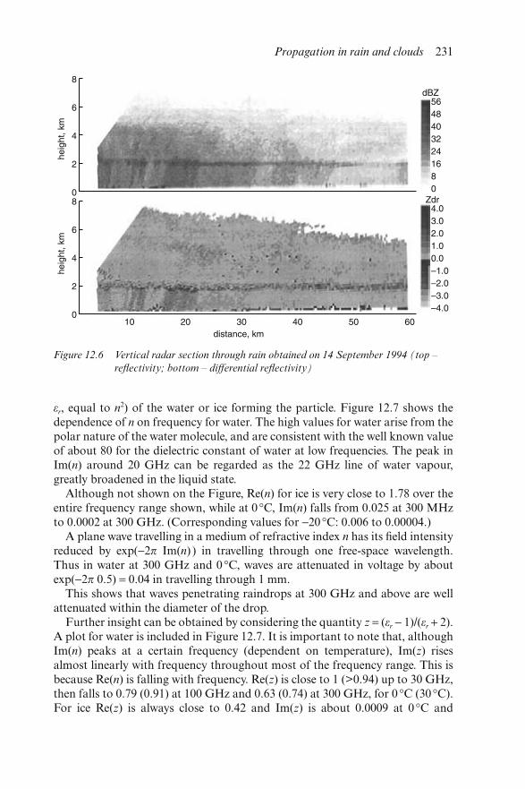
εr, equal to n2) of the water or ice forming the particle. Figure 12.7 shows thedependence of n on frequency for water. The high values for water arise from thepolar nature of the water molecule, and are consistent with the well known valueof about 80 for the dielectric constant of water at low frequencies. The peak inIm(n) around 20 GHz can be regarded as the 22 GHz line of water vapour,greatly broadened in the liquid state.
Although not shown on the Figure, Re(n) for ice is very close to 1.78 over theentire frequency range shown, while at 0 °C, Im(n) falls from 0.025 at 300 MHzto 0.0002 at 300 GHz. (Corresponding values for −20 °C: 0.006 to 0.00004.)
A plane wave travelling in a medium of refractive index n has its field intensityreduced by exp(−2π Im(n) ) in travelling through one free-space wavelength.Thus in water at 300 GHz and 0 °C, waves are attenuated in voltage by aboutexp(−2π 0.5) = 0.04 in travelling through 1 mm.
This shows that waves penetrating raindrops at 300 GHz and above are wellattenuated within the diameter of the drop.
Further insight can be obtained by considering the quantity z = (εr − 1)/(εr + 2).A plot for water is included in Figure 12.7. It is important to note that, althoughIm(n) peaks at a certain frequency (dependent on temperature), Im(z) risesalmost linearly with frequency throughout most of the frequency range. This isbecause Re(n) is falling with frequency. Re(z) is close to 1 (>0.94) up to 30 GHz,then falls to 0.79 (0.91) at 100 GHz and 0.63 (0.74) at 300 GHz, for 0 °C (30 °C).For ice Re(z) is always close to 0.42 and Im(z) is about 0.0009 at 0 °C and
Figure 12.6 Vertical radar section through rain obtained on 14 September 1994 (top –
reflectivity; bottom – differential reflectivity)
Propagation in rain and clouds 231
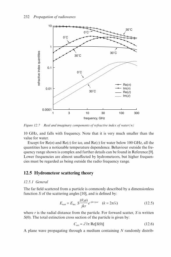
10 GHz, and falls with frequency. Note that it is very much smaller than thevalue for water.
Except for Re(n) and Re(z) for ice, and Re(z) for water below 100 GHz, all thequantities have a noticeable temperature dependence. Behaviour outside the fre-quency range shown is complex and further details can be found in Reference [9].Lower frequencies are almost unaffected by hydrometeors, but higher frequen-cies must be regarded as being outside the radio frequency range.
12.5 Hydrometeor scattering theory
12.5.1 General
The far field scattered from a particle is commonly described by a dimensionlessfunction S of the scattering angles [10], and is defined by:
Escat = Einc. S(θ,φ)
jkre−jkr+jωt (k = 2π/λ) (12.5)
where r is the radial distance from the particle. For forward scatter, S is writtenS(0). The total extinction cross section of the particle is given by:
Cext = λ2/π Re[S(0)] (12.6)
A plane wave propagating through a medium containing N randomly distrib-
Figure 12.7 Real and imaginary components of refractive index of water(n)
232 Propagation of radiowaves
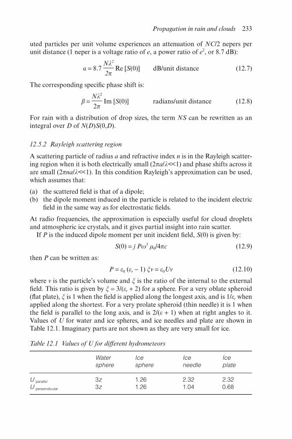
uted particles per unit volume experiences an attenuation of NC/2 nepers perunit distance (1 neper is a voltage ratio of e, a power ratio of e2, or 8.7 dB):
α = 8.7 Nλ2
2π Re [S(0)] dB/unit distance (12.7)
The corresponding specific phase shift is:
β = Nλ2
2π Im [S(0)] radians/unit distance (12.8)
For rain with a distribution of drop sizes, the term NS can be rewritten as anintegral over D of N(D)S(0,D).
12.5.2 Rayleigh scattering region
A scattering particle of radius a and refractive index n is in the Rayleigh scatter-ing region when it is both electrically small (2πa/λ<<1) and phase shifts across itare small (2πna/λ<<1). In this condition Rayleigh’s approximation can be used,which assumes that:
(a) the scattered field is that of a dipole;(b) the dipole moment induced in the particle is related to the incident electric
field in the same way as for electrostatic fields.
At radio frequencies, the approximation is especially useful for cloud dropletsand atmospheric ice crystals, and it gives partial insight into rain scatter.
If P is the induced dipole moment per unit incident field, S(0) is given by:
S(0) = j Pω3 μ0/4πc (12.9)
then P can be written as:
P = ε0 (εr − 1) ξν = ε0Uν (12.10)
where ν is the particle’s volume and ξ is the ratio of the internal to the externalfield. This ratio is given by ξ = 3/(εr + 2) for a sphere. For a very oblate spheroid(flat plate), ξ is 1 when the field is applied along the longest axis, and is 1/εr whenapplied along the shortest. For a very prolate spheroid (thin needle) it is 1 whenthe field is parallel to the long axis, and is 2/(ε + 1) when at right angles to it.Values of U for water and ice spheres, and ice needles and plate are shown inTable 12.1. Imaginary parts are not shown as they are very small for ice.
Table 12.1 Values of U for different hydrometeors
Watersphere
Icesphere
Iceneedle
Iceplate
U parallel 3z 1.26 2.32 2.32U perpendicular 3z 1.26 1.04 0.68
Propagation in rain and clouds 233
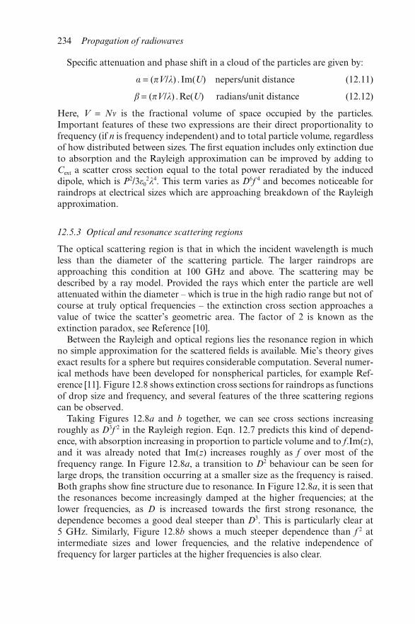
Specific attenuation and phase shift in a cloud of the particles are given by:
α = (πV/λ) . Im(U) nepers/unit distance (12.11)
β = (πV/λ) .Re(U) radians/unit distance (12.12)
Here, V = Nν is the fractional volume of space occupied by the particles.Important features of these two expressions are their direct proportionality tofrequency (if n is frequency independent) and to total particle volume, regardlessof how distributed between sizes. The first equation includes only extinction dueto absorption and the Rayleigh approximation can be improved by adding toCext a scatter cross section equal to the total power reradiated by the induceddipole, which is P2/3ε0
2λ4. This term varies as D6f 4 and becomes noticeable forraindrops at electrical sizes which are approaching breakdown of the Rayleighapproximation.
12.5.3 Optical and resonance scattering regions
The optical scattering region is that in which the incident wavelength is muchless than the diameter of the scattering particle. The larger raindrops areapproaching this condition at 100 GHz and above. The scattering may bedescribed by a ray model. Provided the rays which enter the particle are wellattenuated within the diameter – which is true in the high radio range but not ofcourse at truly optical frequencies – the extinction cross section approaches avalue of twice the scatter’s geometric area. The factor of 2 is known as theextinction paradox, see Reference [10].
Between the Rayleigh and optical regions lies the resonance region in whichno simple approximation for the scattered fields is available. Mie’s theory givesexact results for a sphere but requires considerable computation. Several numer-ical methods have been developed for nonspherical particles, for example Ref-erence [11]. Figure 12.8 shows extinction cross sections for raindrops as functionsof drop size and frequency, and several features of the three scattering regionscan be observed.
Taking Figures 12.8a and b together, we can see cross sections increasingroughly as D3f 2 in the Rayleigh region. Eqn. 12.7 predicts this kind of depend-ence, with absorption increasing in proportion to particle volume and to f.Im(z),and it was already noted that Im(z) increases roughly as f over most of thefrequency range. In Figure 12.8a, a transition to D2 behaviour can be seen forlarge drops, the transition occurring at a smaller size as the frequency is raised.Both graphs show fine structure due to resonance. In Figure 12.8a, it is seen thatthe resonances become increasingly damped at the higher frequencies; at thelower frequencies, as D is increased towards the first strong resonance, thedependence becomes a good deal steeper than D3. This is particularly clear at5 GHz. Similarly, Figure 12.8b shows a much steeper dependence than f 2 atintermediate sizes and lower frequencies, and the relative independence offrequency for larger particles at the higher frequencies is also clear.
234 Propagation of radiowaves
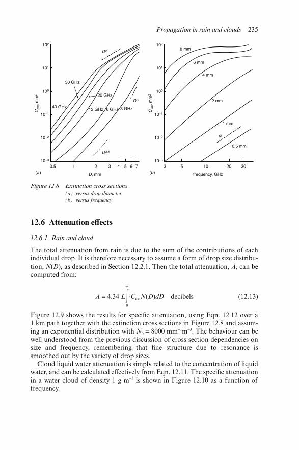
12.6 Attenuation effects
12.6.1 Rain and cloud
The total attenuation from rain is due to the sum of the contributions of eachindividual drop. It is therefore necessary to assume a form of drop size distribu-tion, N(D), as described in Section 12.2.1. Then the total attenuation, A, can becomputed from:
A = 4.34 L�∞
0
⋅CextN(D)dD decibels (12.13)
Figure 12.9 shows the results for specific attenuation, using Eqn. 12.12 over a1 km path together with the extinction cross sections in Figure 12.8 and assum-ing an exponential distribution with N0 = 8000 mm−1m−3. The behaviour can bewell understood from the previous discussion of cross section dependencies onsize and frequency, remembering that fine structure due to resonance issmoothed out by the variety of drop sizes.
Cloud liquid water attenuation is simply related to the concentration of liquidwater, and can be calculated effectively from Eqn. 12.11. The specific attenuationin a water cloud of density 1 g m−3 is shown in Figure 12.10 as a function offrequency.
Figure 12.8 Extinction cross sections(a) versus drop diameter
(b) versus frequency
Propagation in rain and clouds 235
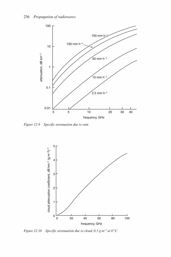
Figure 12.9 Specific attenuation due to rain
Figure 12.10 Specific attenuation due to cloud, 0.5 g m−3 at 0 °C
236 Propagation of radiowaves
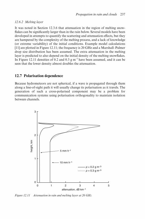
12.6.2 Melting layer
It was noted in Section 12.3.6 that attenuation in the region of melting snow-flakes can be significantly larger than in the rain below. Several models have beendeveloped in attempts to quantify the scattering and attenuation effects, but theyare hampered by the complexity of the melting process, and a lack of knowledge(or extreme variability) of the initial conditions. Example model calculations[11] are plotted in Figure 12.11; the frequency is 20 GHz and a Marshall–Palmerdrop size distribution has been assumed. The extra attenuation in the meltinglayer is predicted to also depend on the initial density of the melting snowflakes.In Figure 12.11 densities of 0.2 and 0.3 g m−3 have been assumed, and it can beseen that the lower density almost doubles the attenuation.
12.7 Polarisation dependence
Because hydrometeors are not spherical, if a wave is propagated through themalong a line-of-sight path it will usually change its polarisation as it travels. Thegeneration of such a cross-polarised component may be a problem forcommunication systems using polarisation orthogonality to maintain isolationbetween channels.
Figure 12.11 Attenuation in rain and melting layer at 20 GHz
Propagation in rain and clouds 237
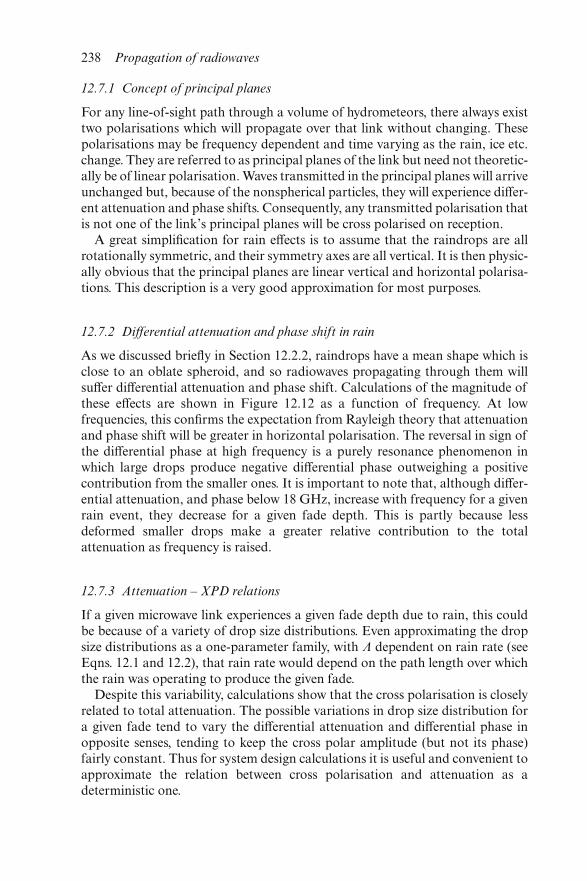
12.7.1 Concept of principal planes
For any line-of-sight path through a volume of hydrometeors, there always existtwo polarisations which will propagate over that link without changing. Thesepolarisations may be frequency dependent and time varying as the rain, ice etc.change. They are referred to as principal planes of the link but need not theoretic-ally be of linear polarisation. Waves transmitted in the principal planes will arriveunchanged but, because of the nonspherical particles, they will experience differ-ent attenuation and phase shifts. Consequently, any transmitted polarisation thatis not one of the link’s principal planes will be cross polarised on reception.
A great simplification for rain effects is to assume that the raindrops are allrotationally symmetric, and their symmetry axes are all vertical. It is then physic-ally obvious that the principal planes are linear vertical and horizontal polarisa-tions. This description is a very good approximation for most purposes.
12.7.2 Differential attenuation and phase shift in rain
As we discussed briefly in Section 12.2.2, raindrops have a mean shape which isclose to an oblate spheroid, and so radiowaves propagating through them willsuffer differential attenuation and phase shift. Calculations of the magnitude ofthese effects are shown in Figure 12.12 as a function of frequency. At lowfrequencies, this confirms the expectation from Rayleigh theory that attenuationand phase shift will be greater in horizontal polarisation. The reversal in sign ofthe differential phase at high frequency is a purely resonance phenomenon inwhich large drops produce negative differential phase outweighing a positivecontribution from the smaller ones. It is important to note that, although differ-ential attenuation, and phase below 18 GHz, increase with frequency for a givenrain event, they decrease for a given fade depth. This is partly because lessdeformed smaller drops make a greater relative contribution to the totalattenuation as frequency is raised.
12.7.3 Attenuation – XPD relations
If a given microwave link experiences a given fade depth due to rain, this couldbe because of a variety of drop size distributions. Even approximating the dropsize distributions as a one-parameter family, with Λ dependent on rain rate (seeEqns. 12.1 and 12.2), that rain rate would depend on the path length over whichthe rain was operating to produce the given fade.
Despite this variability, calculations show that the cross polarisation is closelyrelated to total attenuation. The possible variations in drop size distribution fora given fade tend to vary the differential attenuation and differential phase inopposite senses, tending to keep the cross polar amplitude (but not its phase)fairly constant. Thus for system design calculations it is useful and convenient toapproximate the relation between cross polarisation and attenuation as adeterministic one.
238 Propagation of radiowaves
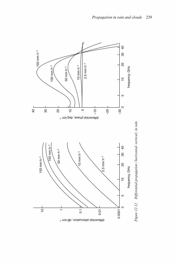
Fig
ure
12.1
2D
iffer
enti
al
pro
paga
tion (
hori
zonta
l–ve
rtic
al)
in r
ain
Propagation in rain and clouds 239
The cross polar magnitude is usually expressed as cross polar discrimination(XPD), defined as the decibel ratio, at the receiving point of a link, of the fieldintensity in the wanted or normal polarisation to that induced by the propaga-tion medium in the orthogonal polarisation. XPD is worst (numerically lowest)when the transmitted polarisation is either circular or is a linear polarisationbisecting the principal planes of the medium.
As a first-order approximation, it can be assumed that the cross polar fieldintensity (voltage) is proportional to the total amount of rain traversed and thusto the total fade. Reverting to the decibel XPD scale this leads to the equation:
XPD = U − 20 log A + I(θ) (12.14)
where A is the fade depth of the copolarised signal in dB, U is a constant for aparticular link frequency. I(θ) is the improvement factor applicable when thetransmitted polarisation is not one of the worst case ones just mentioned. It isapproximately given by 20 log |sin 2θ|, if the transmitted polarisation is linearand makes an angle of θ with the principal planes of the rain medium.
Some experimenters have derived a relationship in which the term 20 log A isreplaced by V log A, V being a second frequency dependent constant. This canmake some allowance for the tendency of deeper fades to be associated withhigher rain rates and thus larger raindrops. Between 8 and 35 GHz, ITU-Rrecommends: U = −30 log f, where f is the link frequency in GHz, with V = 20between 8 and 15 GHz, and V = 23 between 15 and 35 GHz [15]. Relations athigher frequencies appear not to be well established. Note that the f dependenceof U is consistent with the previous comment that differential propagationreduces with f for a given fade depth. Eqn. 12.14 assumes a horizontally propa-gating wave. For an elevated path, the term −40 log(cos elevation) should beadded to XPD because raindrops appear more spherical when viewed at agreater elevation. At 10 GHz, a fade of 15 dB which is quite severe would give aworst case XPD of 6.5 dB at zero elevation.
12.7.4 Rain drop canting angles
It has been shown experimentally that the rain medium exhibits small tilts of itsprincipal planes, so that horizontally and vertically polarised waves do suffermeasurable cross polarisation. This effect is called the canting angle of raindrops. Cross polar measurements [16] suggest that a drop falls so that its sym-metry axis is parallel to the velocity of air flow relative to the drop. If a drop fallsthrough a vertical wind shear, its horizontal velocity is not equal to that of thelocal air and a horizontal component of drag force is produced. The air velocityvector relative to the drop is thus tilted from vertical, hence the symmetry axis isalso tilted.
Calculations show that terrestrial links within about 40 m of the ground couldsee canting angles up to about 5°, and experimental values have been of thisorder. As wind shears reduce with height the model implies equally strongly thattilts seen on earth–satellite paths at elevations of more than a few degrees would
240 Propagation of radiowaves
be unlikely to see angles greater than 1°, which is negligible for practical pur-poses. This has not been conclusively demonstrated in experimental data, due tomeasurement errors.
12.7.5 Ice crystal principal planes
Of the two general types of ice crystal shape thought to affect elevated earth–satellite paths, it is known that plate types generally fall with their flat faces in ahorizontal plane. For a medium of these crystals the principal planes are clearlylinear vertical/linear horizontal.
Needle crystal types are thought to fall with their symmetry axes (which arealso their longest axes) in a horizontal plane. It is also believed that the azimuthsof these long axes may be systematically aligned in one direction by wind shearor sometimes by atmospheric electrostatic fields. The evidence for this comesfrom observations of rapid changes in XPD coinciding with changes in fieldstrength measured by nearby electric field probes [17].
Experimental data suggest that all principal plane angles occur occasionally,but show [18] that they spend about 80 per cent of the time within ±15°of vertical/horizontal when the event is significant. This is consistent with thepicture that needles are usually accompanied by plates at a lower altitude.
12.7.6 Differential phase shift due to ice
Statistics of ice differential phase shift on elevated paths are inferable frommeasurements made at a few sites using satellite beacons. In Europe a typicalvalue exceeded for 0.01 per cent of the time at about 30° elevation would beabout 10° at 12 GHz [18] corresponding to a worst case XPD of 22 dB. Suchstatistics are difficult to relate to any features of the ground rainfall. The phaseshift can, however, be scaled linearly to much higher frequencies still in theRayleigh region. It is also very difficult from any ground-based radio or radarmeasurement to make any detailed inferences about ice particle shapes and sizedistributions. Ice may exhibit resonant scatter in the millimetric region, whichwould be hard to model on the basis of existing data.
12.8 Spatial–temporal structure of rain
12.8.1 Temporal (rainfall rate)
Rainfall rate is obviously the key factor in determining the amount of attenu-ation likely to be suffered by a link. The most widely used statistics are those ofannual rainfall, expressed as rain rate exceeded for a given percentage of theyear. Because of the extreme variability of rainfall statistics at a given location(see Figure 12.13), averages of statistics over many years are recommended. Asthe Figure also shows, even individual gauges can give different results, perhapsdue to calibration differences.
Propagation in rain and clouds 241
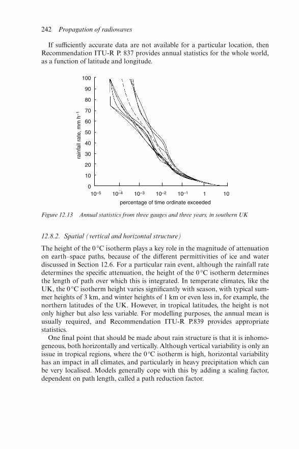
If sufficiently accurate data are not available for a particular location, thenRecommendation ITU-R P. 837 provides annual statistics for the whole world,as a function of latitude and longitude.
12.8.2. Spatial (vertical and horizontal structure)
The height of the 0 °C isotherm plays a key role in the magnitude of attenuationon earth–space paths, because of the different permittivities of ice and waterdiscussed in Section 12.6. For a particular rain event, although the rainfall ratedetermines the specific attenuation, the height of the 0 °C isotherm determinesthe length of path over which this is integrated. In temperate climates, like theUK, the 0 °C isotherm height varies significantly with season, with typical sum-mer heights of 3 km, and winter heights of 1 km or even less in, for example, thenorthern latitudes of the UK. However, in tropical latitudes, the height is notonly higher but also less variable. For modelling purposes, the annual mean isusually required, and Recommendation ITU-R P.839 provides appropriatestatistics.
One final point that should be made about rain structure is that it is inhomo-geneous, both horizontally and vertically. Although vertical variability is only anissue in tropical regions, where the 0 oC isotherm is high, horizontal variabilityhas an impact in all climates, and particularly in heavy precipitation which canbe very localised. Models generally cope with this by adding a scaling factor,dependent on path length, called a path reduction factor.
Figure 12.13 Annual statistics from three gauges and three years, in southern UK
242 Propagation of radiowaves
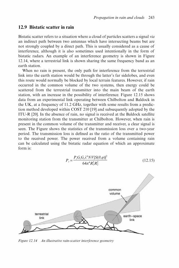
12.9 Bistatic scatter in rain
Bistatic scatter refers to a situation where a cloud of particles scatters a signal via
an indirect path between two antennas which have intersecting beams but arenot strongly coupled by a direct path. This is usually considered as a cause ofinterference, although it is also sometimes used intentionally in the form ofbistatic radars. An example of an interference geometry is shown in Figure12.14, where a terrestrial link is shown sharing the same frequency band as anearth station.
When no rain is present, the only path for interference from the terrestriallink into the earth station would be through the latter’s far sidelobes, and eventhis route would normally be blocked by local terrain features. However, if rainoccurred in the common volume of the two systems, then energy could bescattered from the terrestrial transmitter into the main beam of the earthstation, with an increase in the possibility of interference. Figure 12.15 showsdata from an experimental link operating between Chilbolton and Baldock inthe UK, at a frequency of 11.2 GHz, together with some results from a predic-tion method developed within COST 210 [19] and subsequently adopted by theITU-R [20]. In the absence of rain, no signal is received at the Baldock satellitemonitoring station from the transmitter at Chilbolton. However, when rain ispresent in the common volume of the transmitter and receiver, a clear signal isseen. The Figure shows the statistics of the transmission loss over a two-yearperiod. The transmission loss is defined as the ratio of the transmitted powerto the received power. The power received from a volume containing raincan be calculated using the bistatic radar equation of which an approximateform is:
Pr = PtGtGrλ
4NV|S(θ,φ)|2
64π4R21R
22
(12.15)
Figure 12.14 An illustrative rain-scatter interference geometry
Propagation in rain and clouds 243
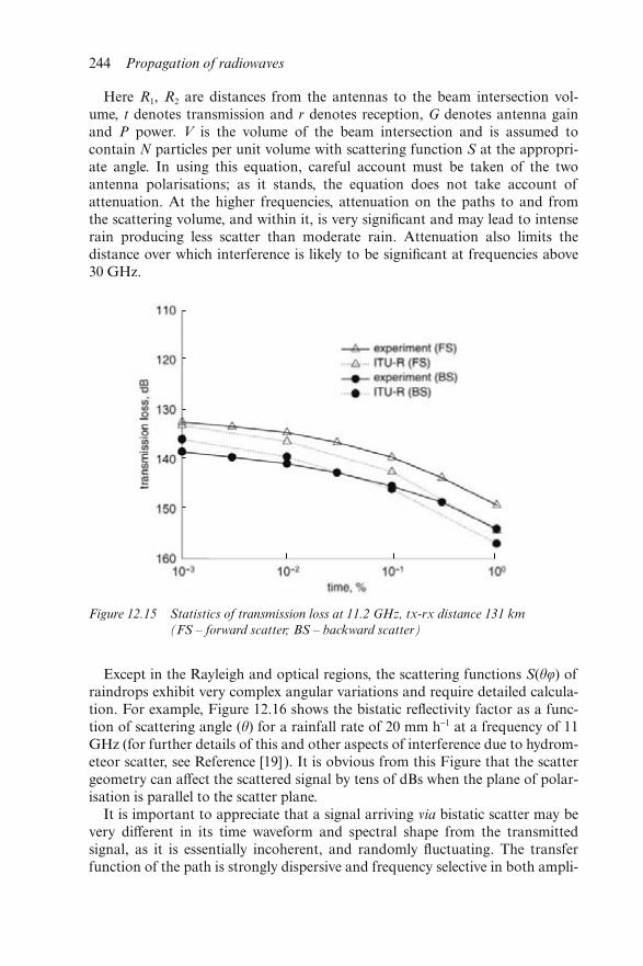
Here R1, R2 are distances from the antennas to the beam intersection vol-ume, t denotes transmission and r denotes reception, G denotes antenna gainand P power. V is the volume of the beam intersection and is assumed tocontain N particles per unit volume with scattering function S at the appropri-ate angle. In using this equation, careful account must be taken of the twoantenna polarisations; as it stands, the equation does not take account ofattenuation. At the higher frequencies, attenuation on the paths to and fromthe scattering volume, and within it, is very significant and may lead to intenserain producing less scatter than moderate rain. Attenuation also limits thedistance over which interference is likely to be significant at frequencies above30 GHz.
Except in the Rayleigh and optical regions, the scattering functions S(θφ) ofraindrops exhibit very complex angular variations and require detailed calcula-tion. For example, Figure 12.16 shows the bistatic reflectivity factor as a func-tion of scattering angle (θ) for a rainfall rate of 20 mm h−1 at a frequency of 11GHz (for further details of this and other aspects of interference due to hydrom-eteor scatter, see Reference [19] ). It is obvious from this Figure that the scattergeometry can affect the scattered signal by tens of dBs when the plane of polar-isation is parallel to the scatter plane.
It is important to appreciate that a signal arriving via bistatic scatter may bevery different in its time waveform and spectral shape from the transmittedsignal, as it is essentially incoherent, and randomly fluctuating. The transferfunction of the path is strongly dispersive and frequency selective in both ampli-
Figure 12.15 Statistics of transmission loss at 11.2 GHz, tx-rx distance 131 km
(FS – forward scatter; BS – backward scatter)
244 Propagation of radiowaves
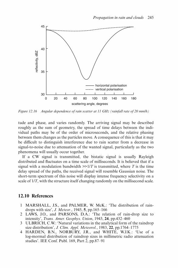
tude and phase, and varies randomly. The arriving signal may be describedroughly as the sum of geometry, the spread of time delays between the indi-vidual paths may be of the order of microseconds, and the relative phasingbetween them changes as the particles move. A consequence of this is that it maybe difficult to distinguish interference due to rain scatter from a decrease insignal-to-noise due to attenuation of the wanted signal, particularly as the twophenomena will usually occur together.
If a CW signal is transmitted, the bistatic signal is usually Rayleighdistributed and fluctuates on a time scale of milliseconds. It is believed that if asignal with a modulation bandwidth >>1/T is transmitted, where T is the timedelay spread of the paths, the received signal will resemble Gaussian noise. Theshort-term spectrum of this noise will display intense frequency selectivity on ascale of 1/T, with the structure itself changing randomly on the millisecond scale.
12.10 References
1 MARSHALL, J.S., and PALMER, W. McK.: ‘The distribution of rain-drops with size’, J. Meteor., 1945, 5, pp.165–166
2 LAWS, J.O., and PARSONS, D.A.: ‘The relation of rain-drop size tointensity’, Trans. Amer. Geophys. Union, 1943, 24, pp.432–460
3 ULBRICH, C.W.: ‘Natural variations in the analytical form of the raindropsize distribution’, J. Clim. Appl. Meteorol., 1983, 22, pp.1764–1775
4 HARDEN, B.N., NORBURY, J.R., and WHITE, W.J.K.: ‘Use of alog-mormal distribution of raindrop sizes in millimetric radio attenuationstudies’. IEE Conf. Publ. 169, Part 2, pp.87–91
Figure 12.16 Angular dependence of rain scatter at 11 GHz (rainfall rate of 20 mm/h)
Propagation in rain and clouds 245
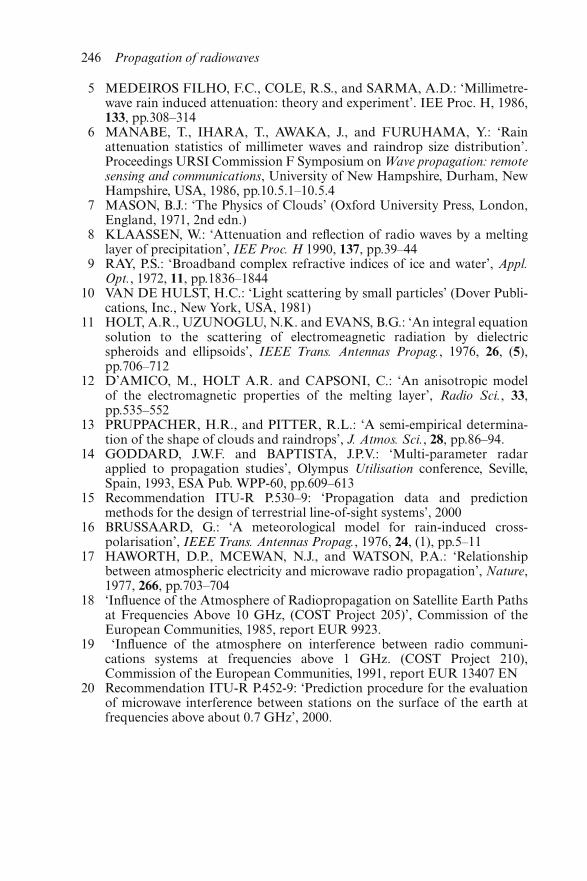
5 MEDEIROS FILHO, F.C., COLE, R.S., and SARMA, A.D.: ‘Millimetre-wave rain induced attenuation: theory and experiment’. IEE Proc. H, 1986,133, pp.308–314
6 MANABE, T., IHARA, T., AWAKA, J., and FURUHAMA, Y.: ‘Rainattenuation statistics of millimeter waves and raindrop size distribution’.Proceedings URSI Commission F Symposium on Wave propagation: remotesensing and communications, University of New Hampshire, Durham, NewHampshire, USA, 1986, pp.10.5.1–10.5.4
7 MASON, B.J.: ‘The Physics of Clouds’ (Oxford University Press, London,England, 1971, 2nd edn.)
8 KLAASSEN, W.: ‘Attenuation and reflection of radio waves by a meltinglayer of precipitation’, IEE Proc. H 1990, 137, pp.39–44
9 RAY, P.S.: ‘Broadband complex refractive indices of ice and water’, Appl.Opt., 1972, 11, pp.1836–1844
10 VAN DE HULST, H.C.: ‘Light scattering by small particles’ (Dover Publi-cations, Inc., New York, USA, 1981)
11 HOLT, A.R., UZUNOGLU, N.K. and EVANS, B.G.: ‘An integral equationsolution to the scattering of electromeagnetic radiation by dielectricspheroids and ellipsoids’, IEEE Trans. Antennas Propag., 1976, 26, (5),pp.706–712
12 D’AMICO, M., HOLT A.R. and CAPSONI, C.: ‘An anisotropic modelof the electromagnetic properties of the melting layer’, Radio Sci., 33,pp.535–552
13 PRUPPACHER, H.R., and PITTER, R.L.: ‘A semi-empirical determina-tion of the shape of clouds and raindrops’, J. Atmos. Sci., 28, pp.86–94.
14 GODDARD, J.W.F. and BAPTISTA, J.P.V.: ‘Multi-parameter radarapplied to propagation studies’, Olympus Utilisation conference, Seville,Spain, 1993, ESA Pub. WPP-60, pp.609–613
15 Recommendation ITU-R P.530–9: ‘Propagation data and predictionmethods for the design of terrestrial line-of-sight systems’, 2000
16 BRUSSAARD, G.: ‘A meteorological model for rain-induced cross-polarisation’, IEEE Trans. Antennas Propag., 1976, 24, (1), pp.5–11
17 HAWORTH, D.P., MCEWAN, N.J., and WATSON, P.A.: ‘Relationshipbetween atmospheric electricity and microwave radio propagation’, Nature,1977, 266, pp.703–704
18 ‘Influence of the Atmosphere of Radiopropagation on Satellite Earth Pathsat Frequencies Above 10 GHz, (COST Project 205)’, Commission of theEuropean Communities, 1985, report EUR 9923.
19 ‘Influence of the atmosphere on interference between radio communi-cations systems at frequencies above 1 GHz. (COST Project 210),Commission of the European Communities, 1991, report EUR 13407 EN
20 Recommendation ITU-R P.452-9: ‘Prediction procedure for the evaluationof microwave interference between stations on the surface of the earth atfrequencies above about 0.7 GHz’, 2000.
246 Propagation of radiowaves
Chapter 13
The propagation aspects of broadcasting atVHF and UHF
J. Middleton
13.1 Introduction
Broadcasting is defined in the ITU Radio Regulations as ‘a radiocommunica-tion service in which the transmissions are intended for direct reception by thegeneral public’. European broadcasting at VHF and UHF takes place in thefrequency ranges shown in Figure 13.1. In the UK, 88–108 MHz is used for FMradio, 218–230 MHz is used for digital radio and 470–860 MHz is used foranalogue and digital television.
The propagation of radiowaves relies on fundamental principles and is
Figure 13.1 Spectrum allocation for VHF/UHF broadcasting
obviously independent of the application. However, the particular require-ments of the broadcaster, where transmitters are required to cover large areas,with little control over the receiving installation, mean that certain aspects ofpropagation have greater significance than for, say, a point-to-point link.
13.2 Limit of service determination
Broadcasters define coverage in terms of field strength, unlike point-to-pointservices where the concept of transmission loss is used. For example, the limit ofservice for television in Band IV is 64 dBμV m−1. Using a typical roof-mountedreceiving antenna, this level of field strength will give sufficient signal at thetelevision receiver to provide a noise-free picture.
This limit of service field strength is based on the requirements of the service.For example, it can be shown that the minimum acceptable signal/noise ratio atthe video output of a domestic television receiver is about 33 dB:
S
N = 20 logPk –Pk picture voltage
RMS noise voltage � = 33 dB
For a vestigial sideband system, the corresponding RF signal/noise = 33 + 8 =41 dB.
The thermal noise voltage at the input of a domestic TV receiver is given by
VN = 10 log[kt0 br] + N + 120 dBμV m−1
where
k = 1.38 × 10⁻²³ the Boltzman constantt0 = 290K reference temperatureb = 5.5 × 10⁶ Hz receiver bandwidthr = 75 Ω receiver input impedanceN = 7 dB receiver noise figure
Therefore VN = 9 dBμV and the minimum voltage at the receiver input:
VR = 9 + 41 = 50 dBμV
This input voltage is related to the field strength E at the receiving antenna bythe following equation:
E = VR + L − G + 20 log f − 33.6 dB
where, in this example:
L = 4 dB feeder lossG = 10 dB antenna gainf = 495 MHz centre of Band IV
248 Propagation of radiowaves
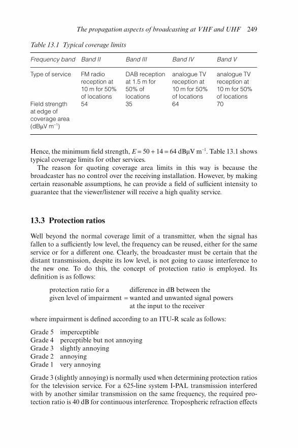
Hence, the minimum field strength, E = 50 + 14 = 64 dBμV m−1. Table 13.1 showstypical coverage limits for other services.
The reason for quoting coverage area limits in this way is because thebroadcaster has no control over the receiving installation. However, by makingcertain reasonable assumptions, he can provide a field of sufficient intensity toguarantee that the viewer/listener will receive a high quality service.
13.3 Protection ratios
Well beyond the normal coverage limit of a transmitter, when the signal hasfallen to a sufficiently low level, the frequency can be reused, either for the sameservice or for a different one. Clearly, the broadcaster must be certain that thedistant transmission, despite its low level, is not going to cause interference tothe new one. To do this, the concept of protection ratio is employed. Itsdefinition is as follows:
protection ratio for a difference in dB between thegiven level of impairment = wanted and unwanted signal powers
at the input to the receiver
where impairment is defined according to an ITU-R scale as follows:
Grade 5 imperceptibleGrade 4 perceptible but not annoyingGrade 3 slightly annoyingGrade 2 annoyingGrade 1 very annoying
Grade 3 (slightly annoying) is normally used when determining protection ratiosfor the television service. For a 625-line system I-PAL transmission interferedwith by another similar transmission on the same frequency, the required pro-tection ratio is 40 dB for continuous interference. Tropospheric refraction effects
Table 13.1 Typical coverage limits
Frequency band Band II Band III Band IV Band V
Type of service FM radioreception at10 m for 50%of locations
DAB receptionat 1.5 m for50% oflocations
analogue TVreception at10 m for 50%of locations
analogue TVreception at10 m for 50%of locations
Field strengthat edge ofcoverage area(dBμV m−1)
54 35 64 70
The propagation aspects of broadcasting at VHF and UHF 249
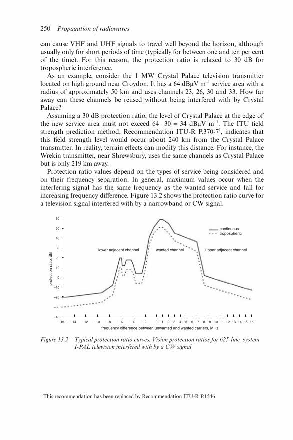
can cause VHF and UHF signals to travel well beyond the horizon, althoughusually only for short periods of time (typically for between one and ten per centof the time). For this reason, the protection ratio is relaxed to 30 dB fortropospheric interference.
As an example, consider the 1 MW Crystal Palace television transmitterlocated on high ground near Croydon. It has a 64 dBμV m−1 service area with aradius of approximately 50 km and uses channels 23, 26, 30 and 33. How faraway can these channels be reused without being interfered with by CrystalPalace?
Assuming a 30 dB protection ratio, the level of Crystal Palace at the edge ofthe new service area must not exceed 64 −30 = 34 dBμV m−1. The ITU fieldstrength prediction method, Recommendation ITU-R P.370-71, indicates thatthis field strength level would occur about 240 km from the Crystal Palacetransmitter. In reality, terrain effects can modify this distance. For instance, theWrekin transmitter, near Shrewsbury, uses the same channels as Crystal Palacebut is only 219 km away.
Protection ratio values depend on the types of service being considered andon their frequency separation. In general, maximum values occur when theinterfering signal has the same frequency as the wanted service and fall forincreasing frequency difference. Figure 13.2 shows the protection ratio curve fora television signal interfered with by a narrowband or CW signal.
Figure 13.2 Typical protection ratio curves. Vision protection ratios for 625-line, system
I-PAL television interfered with by a CW signal
1 This recommendation has been replaced by Recommendation ITU-R P.1546
250 Propagation of radiowaves
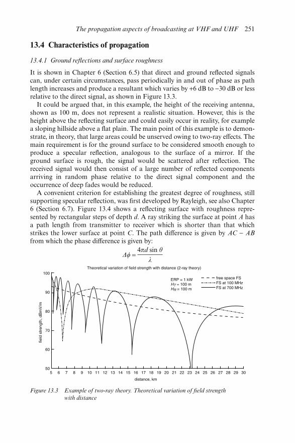
13.4 Characteristics of propagation
13.4.1 Ground reflections and surface roughness
It is shown in Chapter 6 (Section 6.5) that direct and ground reflected signalscan, under certain circumstances, pass periodically in and out of phase as pathlength increases and produce a resultant which varies by +6 dB to −30 dB or lessrelative to the direct signal, as shown in Figure 13.3.
It could be argued that, in this example, the height of the receiving antenna,shown as 100 m, does not represent a realistic situation. However, this is theheight above the reflecting surface and could easily occur in reality, for examplea sloping hillside above a flat plain. The main point of this example is to demon-strate, in theory, that large areas could be unserved owing to two-ray effects. Themain requirement is for the ground surface to be considered smooth enough toproduce a specular reflection, analogous to the surface of a mirror. If theground surface is rough, the signal would be scattered after reflection. Thereceived signal would then consist of a large number of reflected componentsarriving in random phase relative to the direct signal component and theoccurrence of deep fades would be reduced.
A convenient criterion for establishing the greatest degree of roughness, stillsupporting specular reflection, was first developed by Rayleigh, see also Chapter6 (Section 6.7). Figure 13.4 shows a reflecting surface with roughness repre-sented by rectangular steps of depth d. A ray striking the surface at point A hasa path length from transmitter to receiver which is shorter than that whichstrikes the lower surface at point C. The path difference is given by AC − AB
from which the phase difference is given by:
Δ = 4πd sin θ
λ
Figure 13.3 Example of two-ray theory. Theoretical variation of field strength
with distance
The propagation aspects of broadcasting at VHF and UHF 251
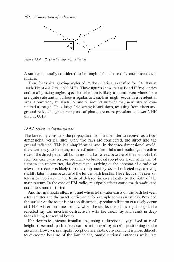
A surface is usually considered to be rough if this phase difference exceeds π/4radians.
Thus, for typical grazing angles of 1°, the criterion is satisfied for d > 10 m at100 MHz or d > 2 m at 600 MHz. These figures show that at Band II frequenciesand small grazing angles, specular reflection is likely to occur, even where thereare quite substantial surface irregularities, such as might occur in a residentialarea. Conversely, at Bands IV and V, ground surfaces may generally be con-sidered as rough. Thus, large field strength variations, resulting from direct andground reflected signals being out of phase, are more prevalent at lower VHFthan at UHF.
13.4.2 Other multipath effects
The foregoing considers the propagation from transmitter to receiver as a two-dimensional vertical slice. Only two rays are considered, the direct and theground reflected. This is a simplification and, in the three-dimensional world,there are likely to be many more reflections from hills and buildings on eitherside of the direct path. Tall buildings in urban areas, because of their smooth flatsurfaces, can cause serious problems to broadcast reception. Even when line ofsight to the transmitter, the direct signal arriving at the antenna of a radio ortelevision receiver is likely to be accompanied by several reflected rays arrivingslightly later in time because of the longer path lengths. The effect can be seen ontelevision receivers in the form of delayed images slightly to the right of themain picture. In the case of FM radio, multipath effects cause the demodulatedaudio to sound distorted.
Another multipath effect is found where tidal water exists on the path betweena transmitter and the target service area, for example across an estuary. Providedthe surface of the water is not too disturbed, specular reflection can easily occurat UHF. At certain times of day, when the sea level is at the right height, thereflected ray can interfere destructively with the direct ray and result in deepfades lasting for several hours.
For domestic antenna installations, using a directional yagi fixed at roofheight, these multipath effects can be minimised by careful positioning of theantenna. However, multipath reception in a mobile environment is more difficultto overcome because of the low height, omnidirectional antennas which are
Figure 13.4 Rayleigh roughness criterion
252 Propagation of radiowaves
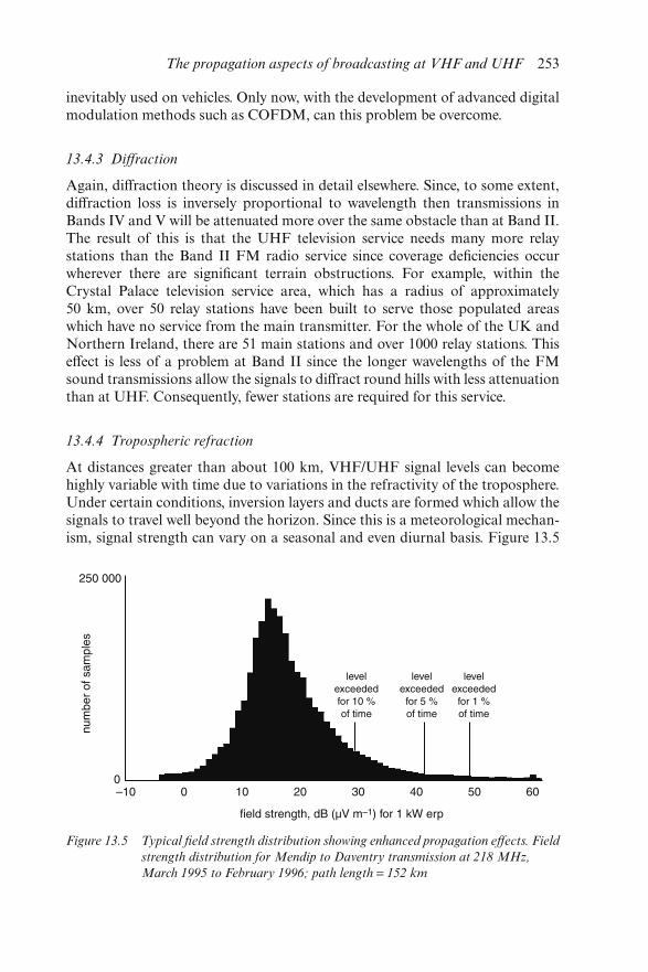
inevitably used on vehicles. Only now, with the development of advanced digitalmodulation methods such as COFDM, can this problem be overcome.
13.4.3 Diffraction
Again, diffraction theory is discussed in detail elsewhere. Since, to some extent,diffraction loss is inversely proportional to wavelength then transmissions inBands IV and V will be attenuated more over the same obstacle than at Band II.The result of this is that the UHF television service needs many more relaystations than the Band II FM radio service since coverage deficiencies occurwherever there are significant terrain obstructions. For example, within theCrystal Palace television service area, which has a radius of approximately50 km, over 50 relay stations have been built to serve those populated areaswhich have no service from the main transmitter. For the whole of the UK andNorthern Ireland, there are 51 main stations and over 1000 relay stations. Thiseffect is less of a problem at Band II since the longer wavelengths of the FMsound transmissions allow the signals to diffract round hills with less attenuationthan at UHF. Consequently, fewer stations are required for this service.
13.4.4 Tropospheric refraction
At distances greater than about 100 km, VHF/UHF signal levels can becomehighly variable with time due to variations in the refractivity of the troposphere.Under certain conditions, inversion layers and ducts are formed which allow thesignals to travel well beyond the horizon. Since this is a meteorological mechan-ism, signal strength can vary on a seasonal and even diurnal basis. Figure 13.5
Figure 13.5 Typical field strength distribution showing enhanced propagation effects. Field
strength distribution for Mendip to Daventry transmission at 218 MHz,
March 1995 to February 1996; path length = 152 km
The propagation aspects of broadcasting at VHF and UHF 253
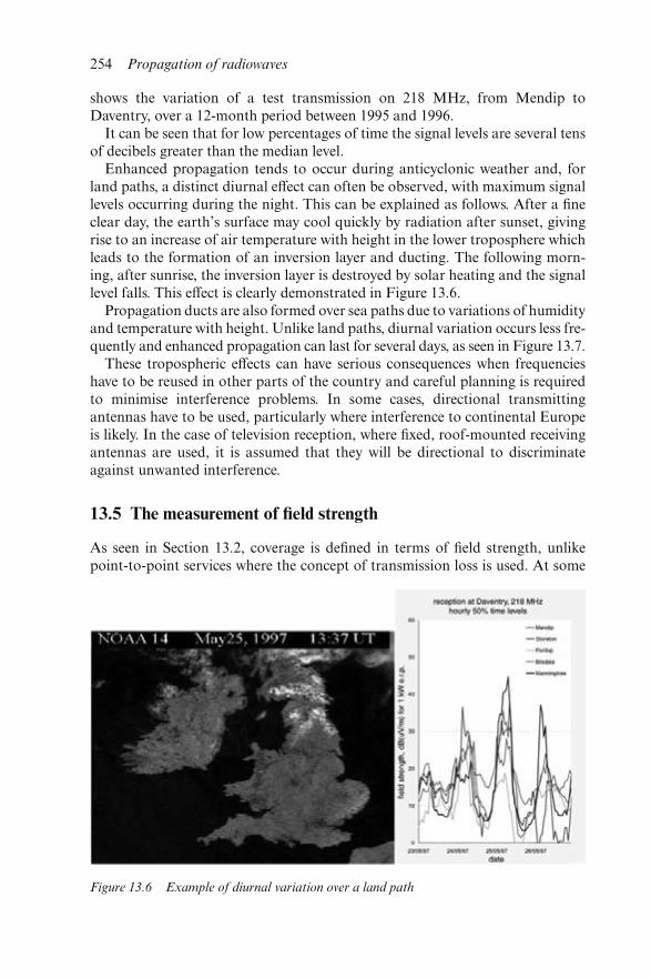
shows the variation of a test transmission on 218 MHz, from Mendip toDaventry, over a 12-month period between 1995 and 1996.
It can be seen that for low percentages of time the signal levels are several tensof decibels greater than the median level.
Enhanced propagation tends to occur during anticyclonic weather and, forland paths, a distinct diurnal effect can often be observed, with maximum signallevels occurring during the night. This can be explained as follows. After a fineclear day, the earth’s surface may cool quickly by radiation after sunset, givingrise to an increase of air temperature with height in the lower troposphere whichleads to the formation of an inversion layer and ducting. The following morn-ing, after sunrise, the inversion layer is destroyed by solar heating and the signallevel falls. This effect is clearly demonstrated in Figure 13.6.
Propagation ducts are also formed over sea paths due to variations of humidityand temperature with height. Unlike land paths, diurnal variation occurs less fre-quently and enhanced propagation can last for several days, as seen in Figure 13.7.
These tropospheric effects can have serious consequences when frequencieshave to be reused in other parts of the country and careful planning is requiredto minimise interference problems. In some cases, directional transmittingantennas have to be used, particularly where interference to continental Europeis likely. In the case of television reception, where fixed, roof-mounted receivingantennas are used, it is assumed that they will be directional to discriminateagainst unwanted interference.
13.5 The measurement of field strength
As seen in Section 13.2, coverage is defined in terms of field strength, unlikepoint-to-point services where the concept of transmission loss is used. At some
Figure 13.6 Example of diurnal variation over a land path
254 Propagation of radiowaves
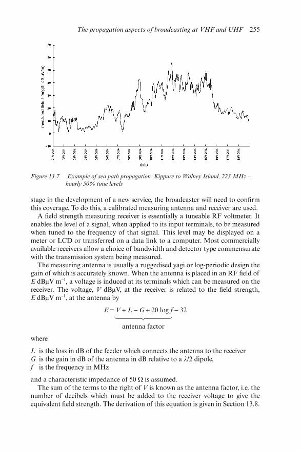
stage in the development of a new service, the broadcaster will need to confirmthis coverage. To do this, a calibrated measuring antenna and receiver are used.
A field strength measuring receiver is essentially a tuneable RF voltmeter. Itenables the level of a signal, when applied to its input terminals, to be measuredwhen tuned to the frequency of that signal. This level may be displayed on ameter or LCD or transferred on a data link to a computer. Most commerciallyavailable receivers allow a choice of bandwidth and detector type commensuratewith the transmission system being measured.
The measuring antenna is usually a ruggedised yagi or log-periodic design thegain of which is accurately known. When the antenna is placed in an RF field ofE dBμV m−1, a voltage is induced at its terminals which can be measured on thereceiver. The voltage, V dBμV, at the receiver is related to the field strength,E dBμV m−1, at the antenna by
E = V + L − G + 20 log f − 32
⎧ ⎪ ⎪ ⎨ ⎪ ⎪ ⎩
antenna factor
where
L is the loss in dB of the feeder which connects the antenna to the receiverG is the gain in dB of the antenna in dB relative to a λ/2 dipole,f is the frequency in MHz
and a characteristic impedance of 50 Ω is assumed.The sum of the terms to the right of V is known as the antenna factor, i.e. the
number of decibels which must be added to the receiver voltage to give theequivalent field strength. The derivation of this equation is given in Section 13.8.
Figure 13.7 Example of sea path propagation. Kippure to Walney Island, 223 MHz –
hourly 50% time levels
The propagation aspects of broadcasting at VHF and UHF 255
Two methods of measurement are normally used. For the television service,where it is assumed that the domestic receiving antenna is roof mounted, themeasuring antenna is mounted on a pneumatic mast so that it can be elevated toa height of 10 m. The field strength is then measured with the vehicle stationaryalthough, at UHF, particularly in urban or suburban areas, the measurementsare made over a short distance to average out any multipath effects. Thismethod, although giving an accurate assessment of the coverage, can be a verytime-consuming process.
For evaluating in-car radio reception, the measuring antenna is usually a λ/4whip mounted on the vehicle roof. The field strength is measured while thevehicle is moving and the results are logged on a computer. Some form ofpositional information can also be fed to the computer either from a GPSreceiver or some other radio-based location system.
13.6 The prediction of field strength
When planning a new service the broadcaster needs to know where to build thetransmitters and what powers to radiate to get the most effective coverage. Wehave seen in Section 13.3 that he also needs to know where he can reuse the samefrequencies without causing interference. To do this some form of field strengthprediction technique is required. There are two approaches to propagationprediction, empirical and deterministic.
A well known empirical method, recommended by the ITU for many years, isITU Recommendation P.370. It has been used for VHF and UHF planning,particularly where coordination is required between neighbouring countries.The method was based on a set of curves of field strength plotted againstdistance, obtained from an extensive measurement campaign. The curvesallowed field strengths to be predicted for 50, 10, 5 and 1 per cent time for landand sea paths. Although path profile information was not essential, accuracywas improved through a series of corrections for which knowledge of the terrainat both ends of the propagation path was required. Although not generallyrenowned for its accuracy of prediction, this method has been widely used fornational and international planning since it had the benefit of impartiality. Simi-lar methods may now be used with the current successor Recommendation,ITU-R P.1546.
The deterministic approach attempts to mathematically model the propaga-tion path and associated propagation conditions. The so-called BBC method isan example of this, and most broadcasting organisations have similar methods.A terrain height database is required from which is constructed a path profile.This determines the existence of sea or land and characterises the terrain intoa series of discrete geometric shapes, i.e. smooth earth, knife edge, wedge orcylinder. A path loss calculation is then made according to how the pro-file approaches or intrudes into the line between the transmitter and receiver.Figure 13.8 shows a typical example.
256 Propagation of radiowaves
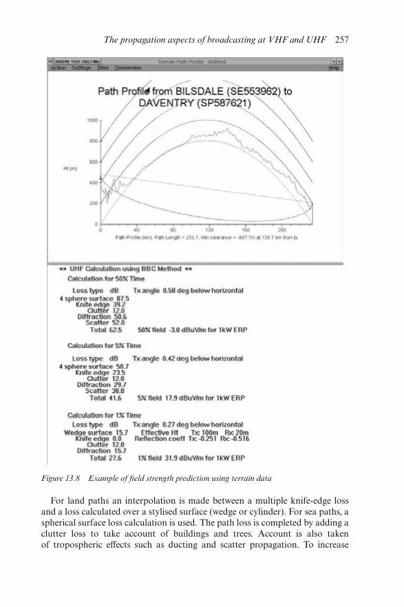
For land paths an interpolation is made between a multiple knife-edge lossand a loss calculated over a stylised surface (wedge or cylinder). For sea paths, aspherical surface loss calculation is used. The path loss is completed by adding aclutter loss to take account of buildings and trees. Account is also takenof tropospheric effects such as ducting and scatter propagation. To increase
Figure 13.8 Example of field strength prediction using terrain data
The propagation aspects of broadcasting at VHF and UHF 257
the accuracy of the results the theoretical calculations are modified by anoptimisation factor based on many field strength measurements made in popu-lated areas. The standard deviation of the prediction error is normally about7 dB.
The deterministic method tends to be more accurate than the empirical onealthough not as much as might be expected. This is mainly because it only modelsa single path between transmitter and receiver. In reality, the level of the receivedsignal is the resultant of many additional signals due to reflections from hills orbuildings. As a result, these programs are used only to provide a rough guide oftransmitter coverage. Their main application is to calculate low-percentage timeinterference levels in conjunction with network planning software.
Nevertheless, modern high-speed computers, with large memories, are enabl-ing new approaches to field strength prediction to be considered, such as theparabolic equation method. This method models the propagation environmentbetween the transmitter and receiver on a three-dimensional basis and has thepotential for making more accurate predictions. However, it may be several yearsbefore such methods are used on a regular basis for planning purposes.
13.7 Digital broadcasting
So far, the discussion has been about conventional analogue broadcasting sys-tems. New digital techniques are now being developed which have the potentialfor greatly improving the quality and efficiency of broadcasting.
13.7.1 DAB
The implementation of digital audio broadcasting (DAB) is well advanced in theUK and uses a COFDM (coded orthogonal frequency division multiplex) sys-tem which has been standardised throughout Europe by the EUREKA 147consortium. UK transmissions are in Band III (218 to 230 MHz) and comprise a1.5 MHz wide block which can carry five high quality audio services.
A fundamental feature of the system is the ability to operate satisfactorily inareas having high levels of multipath propagation. This is achieved by theincorporation of a guard interval in the time domain. Provided the longestmultipath delay time does not significantly exceed this guard interval then allreceived signal components add constructively. Therefore, the system is capableof providing excellent coverage to moving vehicles.
From the viewpoint of signal processing within the receiver, a multipath signalis indistinguishable from another suitably delayed transmission carrying exactlythe same modulation. It follows that a network of DAB transmitters can cover alarge area using a single frequency block without mutual interference. This con-cept of the single frequency network (SFN) makes for high spectral efficiencywhich is ideally suited to national broadcasting.
Another advantage of the SFN is the concept of network gain. This arises
258 Propagation of radiowaves
from the fact that, in many areas, the coverage from adjacent transmitters willoverlap hence signal powers are added in the receiver. There is also a statisticalcomponent due to the location variation distributions of the different fields. Theoverall standard deviation of the composite received signal is less than that ofa single signal. Hence, the power margin to achieve 99 per cent of locationsrelative to, say, 50 per cent coverage is less than for a single transmitter case.
Signals which arrive outside the guard interval will degrade reception of themain signal and this can happen with distant DAB transmissions, albeit fromthe same network, when they are received due to tropospheric refraction. Theeffect will be to cause service areas to shrink slightly. If this becomes a problemin a particular area then, being a single frequency network, the solution isrelatively easy – provide a low power fill-in station to serve that area.
13.7.2 DTT
Digital terrestrial television (DTT) is also being implemented in the UK – thefirst stage of the transmitter network, consisting of 80 transmitters, is nowcomplete. However, unlike DAB, the requirements of the system mean that asingle frequency network is not feasible. Instead, six 8 MHz wide blocks areradiated from each transmitting site on frequencies interleaved with the existingUHF television channels. Each block or multiplex can carry up to five programswith a quality comparable to system I-PAL. Clearly there is potential for inter-ference to and from the existing analogue television transmissions and great carehas gone into defining and measuring the transmitting antenna radiation pat-terns. In some cases, directional antennas having patterns with 20 to 30 dBnotches have been specified.
13.8 Appendix
13.8.1 Field strength measurement and the antenna factor
If we consider a halfwave dipole in an electric field of e V m−1 the voltage inducedacross the terminals of this dipole is e.λ/π V (see Figure 13.9a). The derivation ofthis voltage is given in Section 13.8.2. The equivalent circuit of such an antenna,terminated in a load resistance RL, is shown in Figure 13.9b where RA is theradiation resistance of the antenna.
The voltage across the load, vL is given by:
vL = eλ
π
iRL
RA + RL
V
It is usual to express field strength in dBμV m−1 hence:
VL = E + 20 logλ
π − 20 log(1 +
RA
RL
) dBμV/m
where VL = 20 log vL and E = 20 log e.
The propagation aspects of broadcasting at VHF and UHF 259
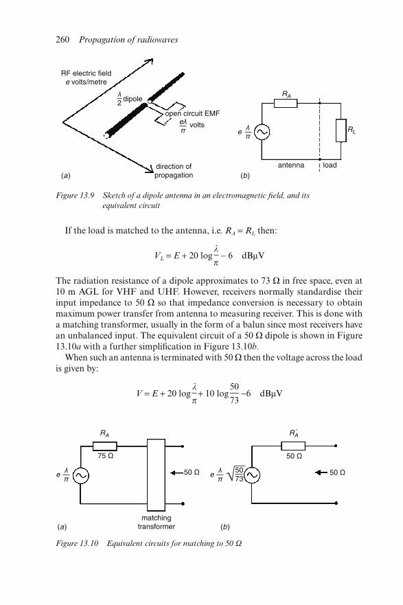
If the load is matched to the antenna, i.e. RA = RL then:
VL = E + 20 logλ
π − 6 dBμV
The radiation resistance of a dipole approximates to 73 Ω in free space, even at10 m AGL for VHF and UHF. However, receivers normally standardise theirinput impedance to 50 Ω so that impedance conversion is necessary to obtainmaximum power transfer from antenna to measuring receiver. This is done witha matching transformer, usually in the form of a balun since most receivers havean unbalanced input. The equivalent circuit of a 50 Ω dipole is shown in Figure13.10a with a further simplification in Figure 13.10b.
When such an antenna is terminated with 50 Ω then the voltage across the loadis given by:
V = E + 20 logλ
π+ 10 log
50
73−6 dBμV
Figure 13.9 Sketch of a dipole antenna in an electromagnetic field, and its
equivalent circuit
Figure 13.10 Equivalent circuits for matching to 50 Ω
260 Propagation of radiowaves
which reduces to:
V = E + 20 logλ
π − 7.6 dBμV
If the antenna in use has a gain G dB relative to a λ/2 dipole and is connected tothe receiver through a feeder with a loss L dB then the equation becomes:
V = E + G − L + 20 logλ
π − 7.6 dBμV
This can be rewritten as:
E = V + L − G + 20 log f − 32 dBμV m−1
where f is the frequency in MHz.The sum of the terms to the right of V is the antenna factor, i.e. the number of
decibels which must be added to the receiver voltage to give the equivalent fieldstrength.
Occasionally, equipment is encountered which has a characteristic impedanceof 75 Ω. In this case the equation becomes: E = V + L − G + 20 log f − 33.7.
13.8.2 The voltage induced in a halfwave dipole
The effective area of an antenna is given by
λ2
4πg m2
where g is the antenna gain relative to an isotropic source.If the antenna is placed in a field whose power density is s W m−2 the power
extracted by the antenna is given by:
p = sλ2
4πg W
A plane wave in free space with a field strength of e V m−1 has a power densitygiven by:
s = e2
120πW m−2
Hence the power received by the antenna is:
p = e2λ2
π2
g
480W
The impedance of a λ/2 dipole in free space is 73 Ω. When connected to amatched load this power will be developed in the load and the equivalentopen-circuit EMF, voc, is related to the received power by:
p = voc
2
4.73W
The propagation aspects of broadcasting at VHF and UHF 261
Hence, for a halfwave dipole (g = 1.64), the open-circuit EMF, voc, can be definedin terms of field strength e by combining these two power relationships to give:
voc = eλ
πV
The ratio λ/π is called the effective length of the halfwave dipole antenna.
262 Propagation of radiowaves
Chapter 14
Propagation aspects of mobile spreadspectrum networks
M.A. Beach and S.A. Allpress
14.1 Introduction to spread spectrum
Spread spectrum has been adopted as the core radio access method in many ofthe third-generation (3G) wireless standards [1], where high capacity networkssupporting multimedia-like services are desired [2]. This selection was based onnumerous research initiatives conducted both privately within numerous organ-isations [3], as well as publicly under initiatives such as the UK DTI LINKprogramme and the European RACE1 and ACTS2 programmes, addressing theselection of the primary air interface technique for the universal mobile tele-communication system (UMTS). Relevant examples include the RACEII [4]ATDMA and CODIT projects, as well as the UK DTI/SERC LINK CDMA [5]programme. More recently, a body called the Third Generation PartnershipProject (3PP) [6] was established with the aim of harmonising the numerousproposals for 3G systems on a global basis.
Networks employing spread spectrum [7] access methods are extremely goodexamples of wideband radio access. Here a narrowband message signal is spreadto a much wider bandwidth than is strictly necessary for RF transmission, thenat the receiver the wideband representation is despread to yield an estimate ofthe original narrowband message signal. Ratios of 10 kHz message bandwidthto several MHz RF channel bandwidth are commonplace in such systems.
There are principally two techniques employed to spread the spectrum. Infrequency hopping (FH) spread spectrum systems the narrowband message sig-nal is modulated with a carrier frequency which is rapidly shifted in discreteincrements in a pattern dictated by a spreading function. This spreading
1 Research into Advanced Communications for Europe2 Advanced Communications Technologies Societies
function is also available at the receiver, and enables it to retune to the correctchannel at the end of each hop. Although the simplest spread spectrum tech-nique to visualise, only a few have attempted to commercially exploit thismethod for personal communication networks. The Geotek [8] system was onesuch embodiment and an analysis of FH propagation in urban cellularenvironments is given by Purle [9]. More recently, FH has been adopted in theBluetooth [10] personal area network (PAN) standard. However, much of thecurrent interest in spread spectrum systems is focused towards the implementa-tion and deployment of direct sequence systems within 3G networks.
Direct sequence (DS) spread spectrum systems take an already modulatednarrowband message signal and apply secondary modulation in the form ofpseudo random noise (PN), thereby spreading the spectrum. This secondarymodulation process is usually implemented in the form of phase shift keying(PSK), and the PN sequence is known as the spreading waveform or sequence,or code. At the receiver, the incoming spread spectrum waveform is multipliedwith an identical synchronised spreading sequence thus resulting in the recoveryof the information or message signal. By associating a unique spreading codewith each user in the network, multiple users can be simultaneously overlaid inboth the time and frequency domains, and the concept of code division multipleaccess (CDMA) realised. Given the considerable interest and investment madeby the early pioneers of this technology (companies such as Qualcomm [11],InterDigital [12] and others [13]), the generic term CDMA has become syn-onymous with cellular systems specially employing the DS spread spectrumtechnique.
The user capacity of all cellular radio access techniques is self interferencelimited [13]. However, CDMA differs from frequency and time multiple accessmethods in as much as the primary source of this interference arises from userssimultaneously occupying the same frequency and time allocations within boththe same cell and cochannel cells. In CDMA terminology this is usually referredto as intra- and intercell interference respectively. The resultant capacity of suchsystems can be significantly increased by employing signal processing techniquesat the receiver which are able to exploit the wideband propagation character-istics of the DS-CDMA channel. It is this fundamental aspect of high capacityCDMA cellular networks that is described in this Chapter.
14.2 Properties of DS-CDMA waveforms
In order to fully understand the propagation and sensitivity analysis of wirelessnetworks employing CDMA access techniques, it is first necessary to considerthe correlation properties of the spreading codes frequently employed in suchsystems. In the context of this discussion it is only necessary to consider theautocorrelation properties [15] of binary pseudo random or m-sequences, asthis gives a measure with which the code can be distinguished from a time-shifted version of itself. M-sequences display an almost ideal two-valued
264 Propagation of radiowaves
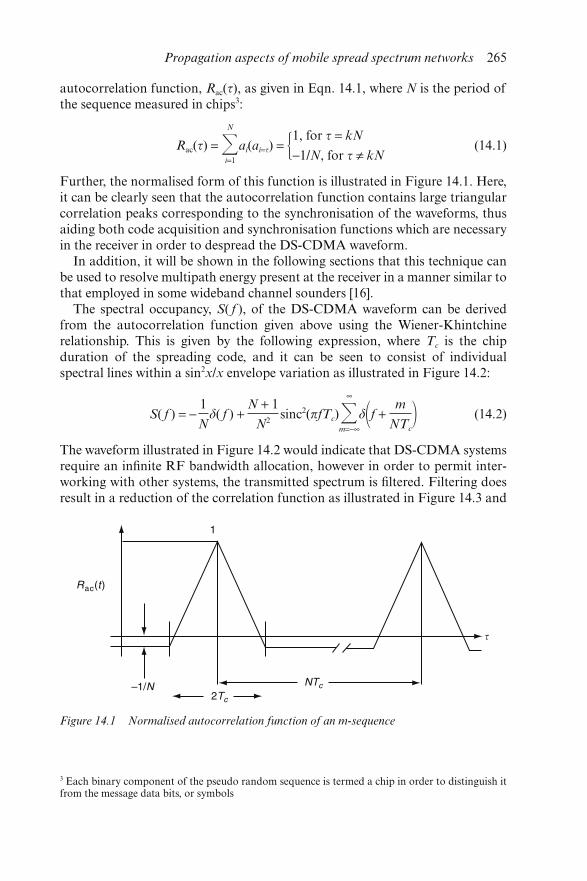
autocorrelation function, Rac(τ), as given in Eqn. 14.1, where N is the period ofthe sequence measured in chips3:
Rac(τ) = �N
i=1
ai(ai=τ) = �1, for τ = kN
−1/N, for τ ≠ kN(14.1)
Further, the normalised form of this function is illustrated in Figure 14.1. Here,it can be clearly seen that the autocorrelation function contains large triangularcorrelation peaks corresponding to the synchronisation of the waveforms, thusaiding both code acquisition and synchronisation functions which are necessaryin the receiver in order to despread the DS-CDMA waveform.
In addition, it will be shown in the following sections that this technique canbe used to resolve multipath energy present at the receiver in a manner similar tothat employed in some wideband channel sounders [16].
The spectral occupancy, S( f ), of the DS-CDMA waveform can be derivedfrom the autocorrelation function given above using the Wiener-Khintchinerelationship. This is given by the following expression, where Tc is the chipduration of the spreading code, and it can be seen to consist of individualspectral lines within a sin2x/x envelope variation as illustrated in Figure 14.2:
S( f ) = −1
Nδ( f ) +
N + 1
N2sinc2(πfTc)�
∞
m=−∞
δ�f + m
NTc� (14.2)
The waveform illustrated in Figure 14.2 would indicate that DS-CDMA systemsrequire an infinite RF bandwidth allocation, however in order to permit inter-working with other systems, the transmitted spectrum is filtered. Filtering doesresult in a reduction of the correlation function as illustrated in Figure 14.3 and
Figure 14.1 Normalised autocorrelation function of an m-sequence
3 Each binary component of the pseudo random sequence is termed a chip in order to distinguish itfrom the message data bits, or symbols
Propagation aspects of mobile spread spectrum networks 265
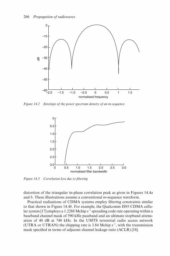
distortion of the triangular in-phase correlation peak as given in Figures 14.4a
and b. These illustrations assume a conventional m-sequence waveform.Practical realisations of CDMA systems employ filtering constraints similar
to that shown in Figure 14.4b. For example, the Qualcomm IS95 CDMA cellu-lar system [17] employs a 1.2288 Mchip s−1 spreading code rate operating within abaseband channel mask of 590 kHz passband and an ultimate stopband attenu-ation of 40 dB at 740 kHz. In the UMTS terrestrial radio access network(UTRA or UTRAN) the chipping rate is 3.84 Mchip s−1, with the transmissionmask specified in terms of adjacent channel leakage ratio (ACLR) [18].
Figure 14.2 Envelope of the power spectrum density of an m-sequence
Figure 14.3 Correlation loss due to filtering
266 Propagation of radiowaves
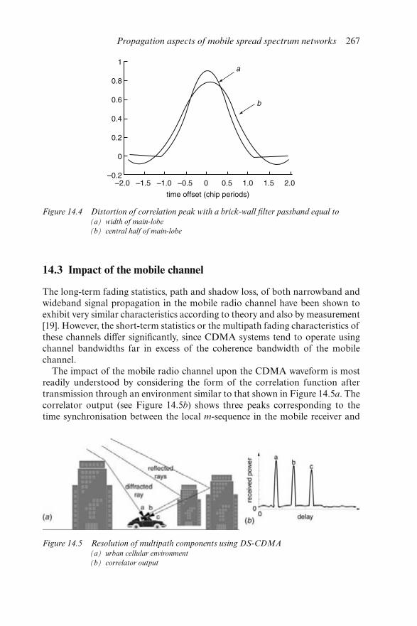
14.3 Impact of the mobile channel
The long-term fading statistics, path and shadow loss, of both narrowband andwideband signal propagation in the mobile radio channel have been shown toexhibit very similar characteristics according to theory and also by measurement[19]. However, the short-term statistics or the multipath fading characteristics ofthese channels differ significantly, since CDMA systems tend to operate usingchannel bandwidths far in excess of the coherence bandwidth of the mobilechannel.
The impact of the mobile radio channel upon the CDMA waveform is mostreadily understood by considering the form of the correlation function aftertransmission through an environment similar to that shown in Figure 14.5a. Thecorrelator output (see Figure 14.5b) shows three peaks corresponding to thetime synchronisation between the local m-sequence in the mobile receiver and
Figure 14.4 Distortion of correlation peak with a brick-wall filter passband equal to(a) width of main-lobe
(b) central half of main-lobe
Figure 14.5 Resolution of multipath components using DS-CDMA(a) urban cellular environment
(b) correlator output
Propagation aspects of mobile spread spectrum networks 267
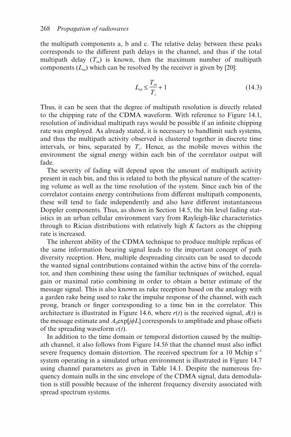
the multipath components a, b and c. The relative delay between these peakscorresponds to the different path delays in the channel, and thus if the totalmultipath delay (Tm) is known, then the maximum number of multipathcomponents (Lm) which can be resolved by the receiver is given by [20]:
Lm ≤ Tm
Tc
+ 1 (14.3)
Thus, it can be seen that the degree of multipath resolution is directly relatedto the chipping rate of the CDMA waveform. With reference to Figure 14.1,resolution of individual multipath rays would be possible if an infinite chippingrate was employed. As already stated, it is necessary to bandlimit such systems,and thus the multipath activity observed is clustered together in discrete timeintervals, or bins, separated by Tc. Hence, as the mobile moves within theenvironment the signal energy within each bin of the correlator output willfade.
The severity of fading will depend upon the amount of multipath activitypresent in each bin, and this is related to both the physical nature of the scatter-ing volume as well as the time resolution of the system. Since each bin of thecorrelator contains energy contributions from different multipath components,these will tend to fade independently and also have different instantaneousDoppler components. Thus, as shown in Section 14.5, the bin level fading stat-istics in an urban cellular environment vary from Rayleigh-like characteristicsthrough to Rician distributions with relatively high K factors as the chippingrate is increased.
The inherent ability of the CDMA technique to produce multiple replicas ofthe same information bearing signal leads to the important concept of pathdiversity reception. Here, multiple despreading circuits can be used to decodethe wanted signal contributions contained within the active bins of the correla-tor, and then combining these using the familiar techniques of switched, equalgain or maximal ratio combining in order to obtain a better estimate of themessage signal. This is also known as rake reception based on the analogy witha garden rake being used to rake the impulse response of the channel, with eachprong, branch or finger corresponding to a time bin in the correlator. Thisarchitecture is illustrated in Figure 14.6, where r(t) is the received signal, d(t) isthe message estimate and A0exp[jL] corresponds to amplitude and phase offsetsof the spreading waveform c(t).
In addition to the time domain or temporal distortion caused by the multip-ath channel, it also follows from Figure 14.5b that the channel must also inflictsevere frequency domain distortion. The received spectrum for a 10 Mchip s−1
system operating in a simulated urban environment is illustrated in Figure 14.7using channel parameters as given in Table 14.1. Despite the numerous fre-quency domain nulls in the sinc envelope of the CDMA signal, data demodula-tion is still possible because of the inherent frequency diversity associated withspread spectrum systems.
268 Propagation of radiowaves
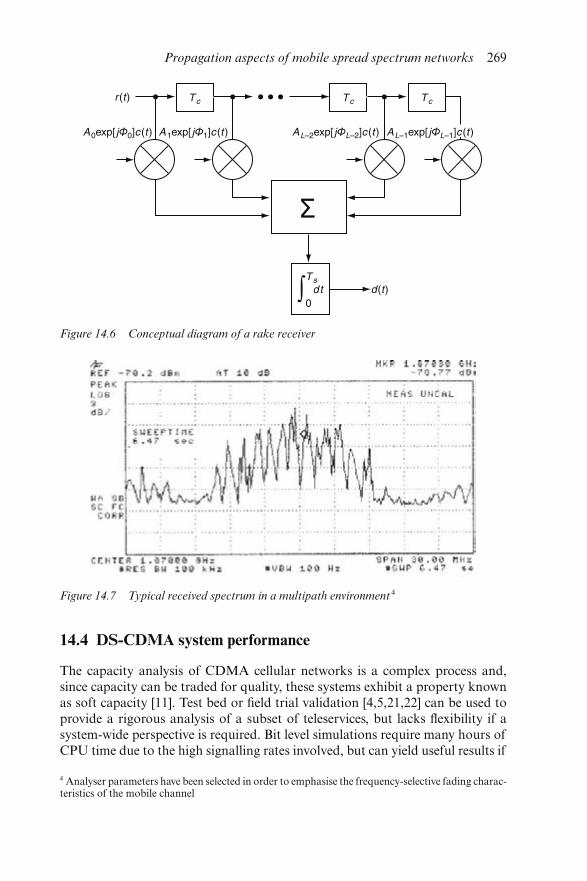
14.4 DS-CDMA system performance
The capacity analysis of CDMA cellular networks is a complex process and,since capacity can be traded for quality, these systems exhibit a property knownas soft capacity [11]. Test bed or field trial validation [4,5,21,22] can be used toprovide a rigorous analysis of a subset of teleservices, but lacks flexibility if asystem-wide perspective is required. Bit level simulations require many hours ofCPU time due to the high signalling rates involved, but can yield useful results if
Figure 14.6 Conceptual diagram of a rake receiver
Figure 14.7 Typical received spectrum in a multipath environment 4
4 Analyser parameters have been selected in order to emphasise the frequency-selective fading charac-teristics of the mobile channel
Propagation aspects of mobile spread spectrum networks 269
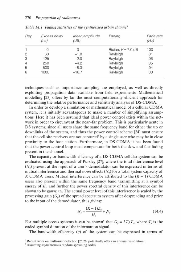
techniques such as importance sampling are employed, as well as directlyexploiting propagation data available from field experiments. Mathematicalmodelling [23] offers by far the most computationally efficient approach fordetermining the relative performance and sensitivity analysis of DS-CDMA.
In order to develop a simulation or mathematical model of a cellular CDMAsystem, it is initially advantageous to make a number of simplifying assump-tions. Here it has been assumed that ideal power control exists within the net-work in order to circumvent the near–far problem. This is particularly acute inDS systems, since all users share the same frequency band for either the up ordownlinks of the system, and thus the power control scheme [24] must ensurethat the cell site receivers are not captured5 by a single user who may be in closeproximity to the base station. Furthermore, in DS-CDMA it has been foundthat the power control loop must compensate for both the slow and fast fadingpresent in the channel.
The capacity or bandwidth efficiency of a DS-CDMA cellular system can beevaluated using the approach of Pursley [27], where the total interference level(NI) present at the input of a user’s demodulator can be expressed in terms ofmutual interference and thermal noise effects (N0) for a total system capacity ofK CDMA users. Mutual interference can be attributed to the (K − 1) CDMAusers also present within the same frequency band transmitting at a symbolenergy of Es, and further the power spectral density of this interference can beshown to be gaussian. The actual power level of this interference is scaled by theprocessing gain (Gp) of the spread spectrum system after despreading and priorto the input of the demodulator, thus giving:
NI = (K − 1)Es
Gp
+ N0 (14.4)
For multiple access systems it can be shown6 that Gp = 3Ts/Tc, where Ts is thecoded symbol duration of the information signal.
The bandwidth efficiency (η) of the system can be expressed in terms of
Table 14.1 Fading statistics of the synthesised urban channel
Ray Excess delay(ns)
Mean amplitude(dB)
Fading Fade rate(Hz)
1 0 0 Rician, K = 7.0 dB 1002 60 −1.0 Rayleigh 313 125 −2.0 Rayleigh 964 250 −4.2 Rayleigh 355 500 −8.3 Rayleigh 946 1000 −16.7 Rayleigh 80
5 Recent work on multi-user detection [25,26] potentially offers an alternative solution6 Assuming asynchronous random spreading codes
270 Propagation of radiowaves
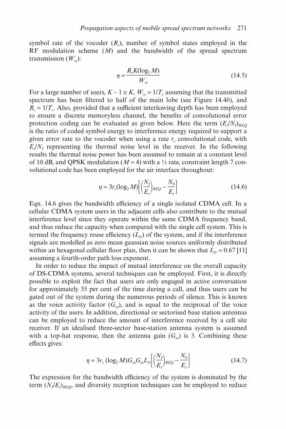
symbol rate of the vocoder (Rs), number of symbol states employed in theRF modulation scheme (M) and the bandwidth of the spread spectrumtransmission (Wss):
η = RsK(log2 M)
Wss
(14.5)
For a large number of users, K − 1 ≅ K, Wss = 1/Tc assuming that the transmittedspectrum has been filtered to half of the main lobe (see Figure 14.4b), andRs = 1/Ts. Also, provided that a sufficient interleaving depth has been employedto ensure a discrete memoryless channel, the benefits of convolutional errorprotection coding can be evaluated as given below. Here the term (Es/NI)REQ
is the ratio of coded symbol energy to interference energy required to support agiven error rate to the vocoder when using a rate rc convolutional code, withEs/NI representing the thermal noise level in the receiver. In the followingresults the thermal noise power has been assumed to remain at a constant levelof 10 dB, and QPSK modulation (M = 4) with a ½ rate, constraint length 7 con-volutional code has been employed for the air interface throughout:
η ≈ 3rc(log2 M)�NI
Es�REQ −
N0
Es� (14.6)
Eqn. 14.6 gives the bandwidth efficiency of a single isolated CDMA cell. In acellular CDMA system users in the adjacent cells also contribute to the mutualinterference level since they operate within the same CDMA frequency band,and thus reduce the capacity when compared with the single cell system. This istermed the frequency reuse efficiency (Lfr) of the system, and if the interferencesignals are modelled as zero mean gaussian noise sources uniformly distributedwithin an hexagonal cellular floor plan, then it can be shown that Lfr = 0.67 [11]assuming a fourth-order path loss exponent.
In order to reduce the impact of mutual interference on the overall capacityof DS-CDMA systems, several techniques can be employed. First, it is directlypossible to exploit the fact that users are only engaged in active conversationfor approximately 35 per cent of the time during a call, and thus users can begated out of the system during the numerous periods of silence. This is knownas the voice activity factor (Gva), and is equal to the reciprocal of the voiceactivity of the users. In addition, directional or sectorised base station antennascan be employed to reduce the amount of interference received by a cell sitereceiver. If an idealised three-sector base-station antenna system is assumedwith a top-hat response, then the antenna gain (Gsa) is 3. Combining theseeffects gives:
η ≈ 3rc (log2 M)GvaGsaLfr�NI
Es�REQ −
N0
Es� (14.7)
The expression for the bandwidth efficiency of the system is dominated by theterm (NI/Es)REQ, and diversity reception techniques can be employed to reduce
Propagation aspects of mobile spread spectrum networks 271

the symbol energy necessary to maintain a given bit error rate (BER), and thusenhance the capacity of the network. In particular, CDMA receivers make useof path diversity reception techniques as illustrated in Figure 14.5, and using theconcept of the coded channel described by Simon [20], the bandwidth efficiencyof a CDMA system can be calculated including the effects of diversity receptionmethods operating in both log-normal Rayleigh and log-normal Rician mobileradio channels [28].
Figure 14.8 gives the BER performance versus Es/NI for varying orders ofinternal diversity while operating in a log-normal Rayleigh channel with astandard deviation of 8 dB. In these results the diversity branches have beencombined using maximal ratio combining (MRC), and it can be seen for a fixedBER that increasing the number of diversity branches results in a considerablereduction of the required Es/NI.
Figure 14.9 illustrates the BER performance versus Es/NI when equal gaincombining (EGC) is employed for a system operating under the same channelconditions as given in Figure 14.8. Again, it can be seen that there are consider-able benefits to be obtained from employing diversity reception techniques, andwhen comparing MRC against EGC there is an approximate power saving of3 dB in favour of MRC for fifth-order path diversity at a BER of 10−3.
Figure 14.10 gives the bandwidth efficiency versus diversity order for bothMRC and EGC architectures operating in the log-normal Rayleigh channel fora BER of 10−3, assuming no base station sectorisation (Gsa = 1). Again, thebenefits of employing MRC combining against EGC can be clearly seen, andalso that there are considerable benefits to be attained in terms of capacityenhancement when employing up to four diversity branches, whereas increasing
Figure 14.8 BER versus Es/NI for MRC operation in a log-normal Rayleigh channel
272 Propagation of radiowaves
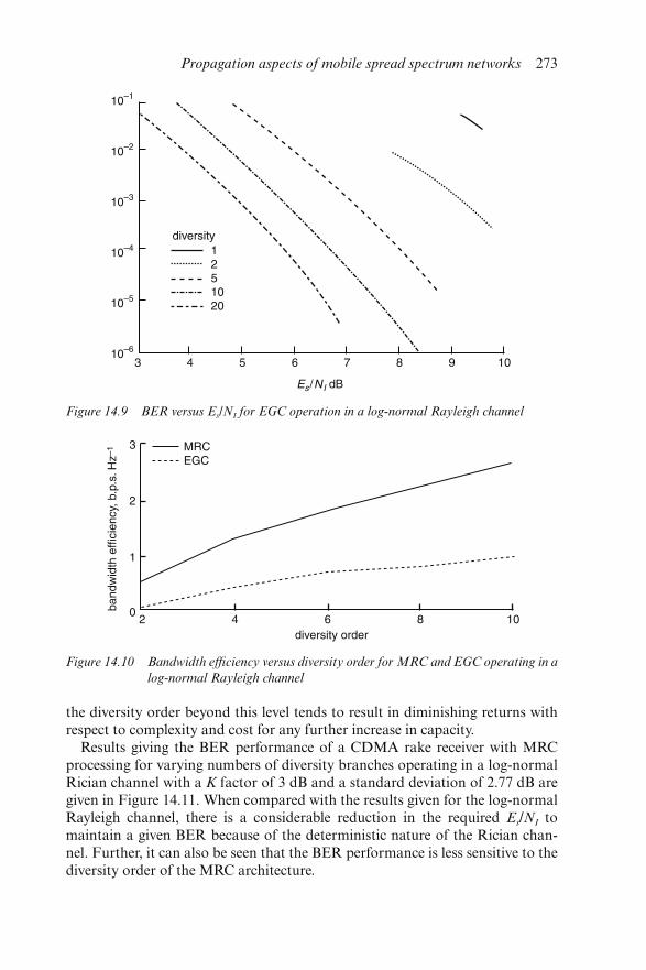
the diversity order beyond this level tends to result in diminishing returns withrespect to complexity and cost for any further increase in capacity.
Results giving the BER performance of a CDMA rake receiver with MRCprocessing for varying numbers of diversity branches operating in a log-normalRician channel with a K factor of 3 dB and a standard deviation of 2.77 dB aregiven in Figure 14.11. When compared with the results given for the log-normalRayleigh channel, there is a considerable reduction in the required Es/NI tomaintain a given BER because of the deterministic nature of the Rician chan-nel. Further, it can also be seen that the BER performance is less sensitive to thediversity order of the MRC architecture.
Figure 14.9 BER versus Es/NI for EGC operation in a log-normal Rayleigh channel
Figure 14.10 Bandwidth efficiency versus diversity order for MRC and EGC operating in a
log-normal Rayleigh channel
Propagation aspects of mobile spread spectrum networks 273
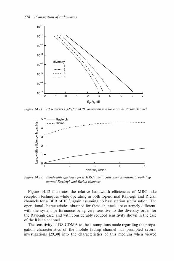
Figure 14.12 illustrates the relative bandwidth efficiencies of MRC rakereception techniques while operating in both log-normal Rayleigh and Ricianchannels for a BER of 10−3, again assuming no base station sectorisation. Theoperational characteristics obtained for these channels are extremely different,with the system performance being very sensitive to the diversity order forthe Rayleigh case, and with considerably reduced sensitivity shown in the caseof the Rician channel.
The sensitivity of DS-CDMA to the assumptions made regarding the propa-gation characteristics of the mobile fading channel has prompted severalinvestigations [29,30] into the characteristics of this medium when viewed
Figure 14.11 BER versus Es/NI for MRC operation in a log-normal Rician channel
Figure 14.12 Bandwidth efficiency for a MRC rake architecture operating in both log-
normal Rayleigh and Rician channels
274 Propagation of radiowaves
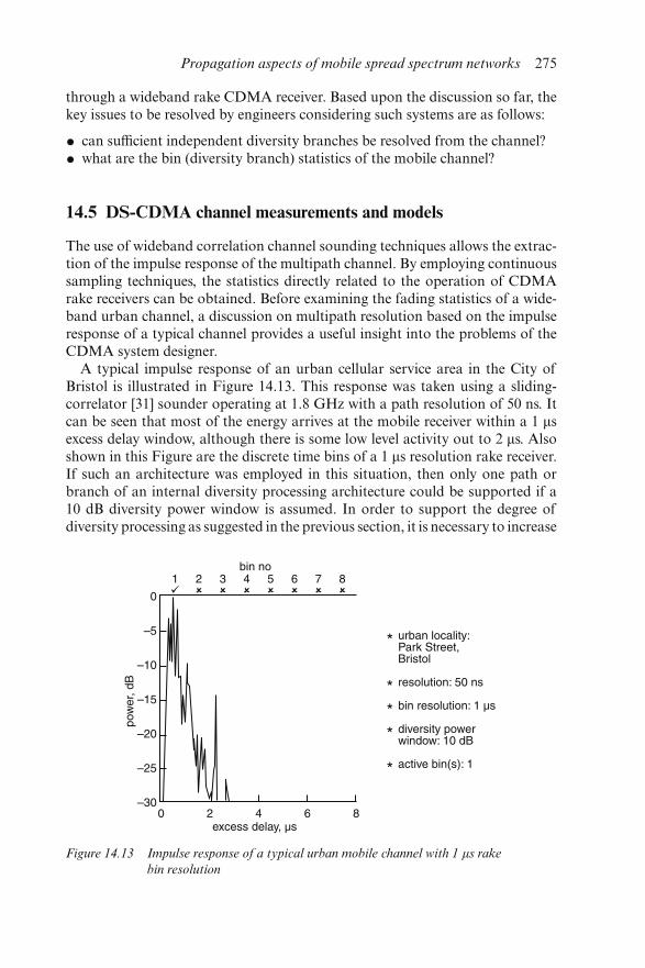
through a wideband rake CDMA receiver. Based upon the discussion so far, thekey issues to be resolved by engineers considering such systems are as follows:
• can sufficient independent diversity branches be resolved from the channel?
• what are the bin (diversity branch) statistics of the mobile channel?
14.5 DS-CDMA channel measurements and models
The use of wideband correlation channel sounding techniques allows the extrac-tion of the impulse response of the multipath channel. By employing continuoussampling techniques, the statistics directly related to the operation of CDMArake receivers can be obtained. Before examining the fading statistics of a wide-band urban channel, a discussion on multipath resolution based on the impulseresponse of a typical channel provides a useful insight into the problems of theCDMA system designer.
A typical impulse response of an urban cellular service area in the City ofBristol is illustrated in Figure 14.13. This response was taken using a sliding-correlator [31] sounder operating at 1.8 GHz with a path resolution of 50 ns. Itcan be seen that most of the energy arrives at the mobile receiver within a 1 μsexcess delay window, although there is some low level activity out to 2 μs. Alsoshown in this Figure are the discrete time bins of a 1 μs resolution rake receiver.If such an architecture was employed in this situation, then only one path orbranch of an internal diversity processing architecture could be supported if a10 dB diversity power window is assumed. In order to support the degree ofdiversity processing as suggested in the previous section, it is necessary to increase
Figure 14.13 Impulse response of a typical urban mobile channel with 1 μs rake
bin resolution
Propagation aspects of mobile spread spectrum networks 275
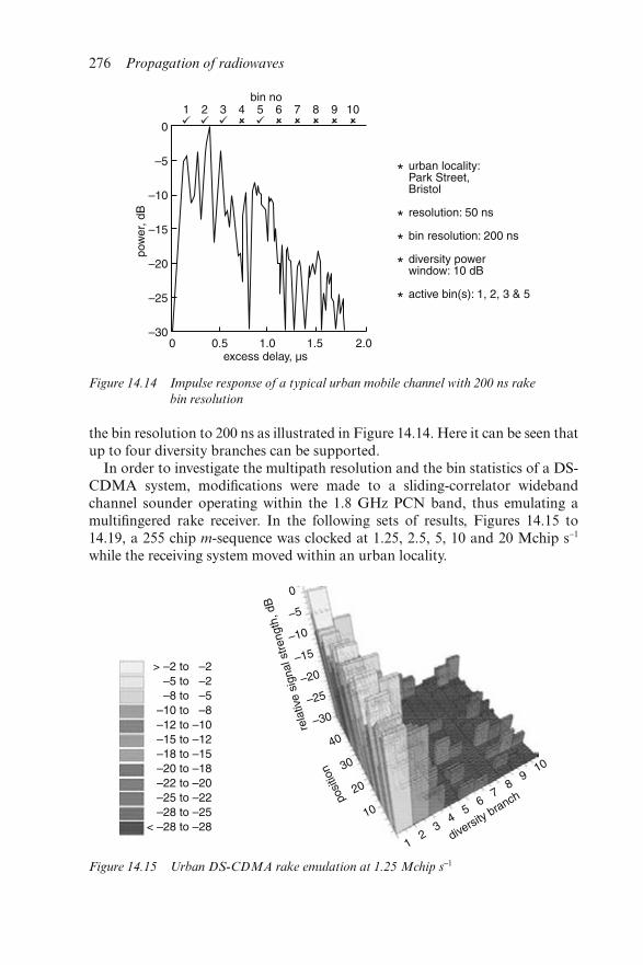
the bin resolution to 200 ns as illustrated in Figure 14.14. Here it can be seen thatup to four diversity branches can be supported.
In order to investigate the multipath resolution and the bin statistics of a DS-CDMA system, modifications were made to a sliding-correlator widebandchannel sounder operating within the 1.8 GHz PCN band, thus emulating amultifingered rake receiver. In the following sets of results, Figures 14.15 to14.19, a 255 chip m-sequence was clocked at 1.25, 2.5, 5, 10 and 20 Mchip s−1
while the receiving system moved within an urban locality.
Figure 14.14 Impulse response of a typical urban mobile channel with 200 ns rake
bin resolution
Figure 14.15 Urban DS-CDMA rake emulation at 1.25 Mchip s−1
276 Propagation of radiowaves
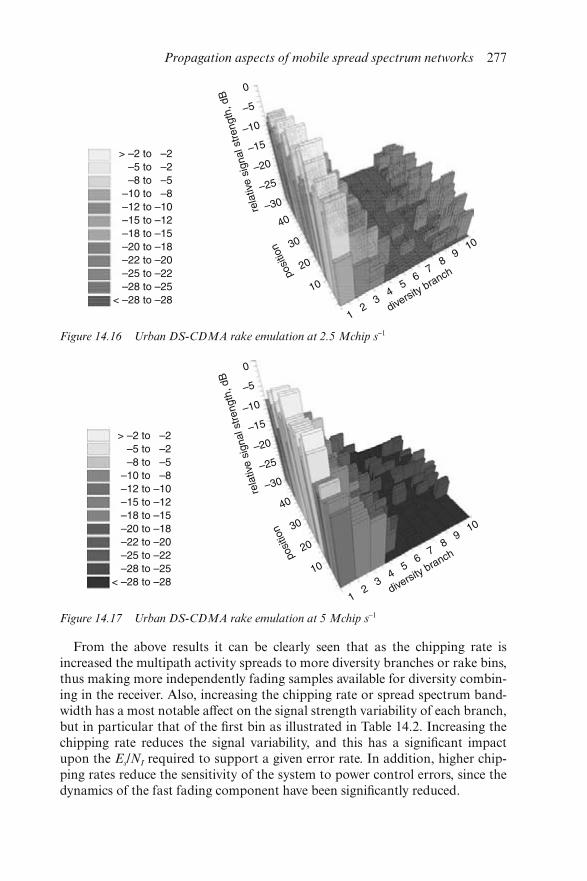
From the above results it can be clearly seen that as the chipping rate isincreased the multipath activity spreads to more diversity branches or rake bins,thus making more independently fading samples available for diversity combin-ing in the receiver. Also, increasing the chipping rate or spread spectrum band-width has a most notable affect on the signal strength variability of each branch,but in particular that of the first bin as illustrated in Table 14.2. Increasing thechipping rate reduces the signal variability, and this has a significant impactupon the Es/NI required to support a given error rate. In addition, higher chip-ping rates reduce the sensitivity of the system to power control errors, since thedynamics of the fast fading component have been significantly reduced.
Figure 14.16 Urban DS-CDMA rake emulation at 2.5 Mchip s−1
Figure 14.17 Urban DS-CDMA rake emulation at 5 Mchip s−1
Propagation aspects of mobile spread spectrum networks 277
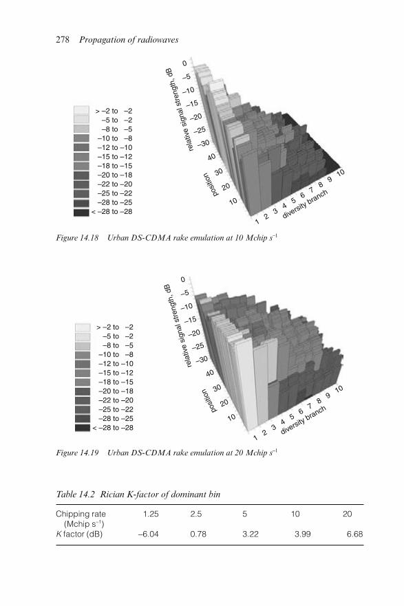
Figure 14.18 Urban DS-CDMA rake emulation at 10 Mchip s−1
Figure 14.19 Urban DS-CDMA rake emulation at 20 Mchip s−1
Table 14.2 Rician K-factor of dominant bin
Chipping rate(Mchip s−1)
1.25 2.5 5 10 20
K factor (dB) −6.04 0.78 3.22 3.99 6.68
278 Propagation of radiowaves
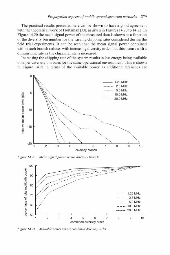
The practical results presented here can be shown to have a good agreementwith the theoretical work of Holtzman [33], as given in Figures 14.20 to 14.22. InFigure 14.20 the mean signal power of the measured data is shown as a functionof the diversity bin number for the varying chipping rates considered during thefield trial experiments. It can be seen that the mean signal power containedwithin each branch reduces with increasing diversity order, but this occurs with adiminishing rate as the chipping rate is increased.
Increasing the chipping rate of the system results in less energy being availableon a per diversity bin basis for the same operational environment. This is shownin Figure 14.21 in terms of the available power as additional branches are
Figure 14.20 Mean signal power versus diversity branch
Figure 14.21 Available power versus combined diversity order
Propagation aspects of mobile spread spectrum networks 279
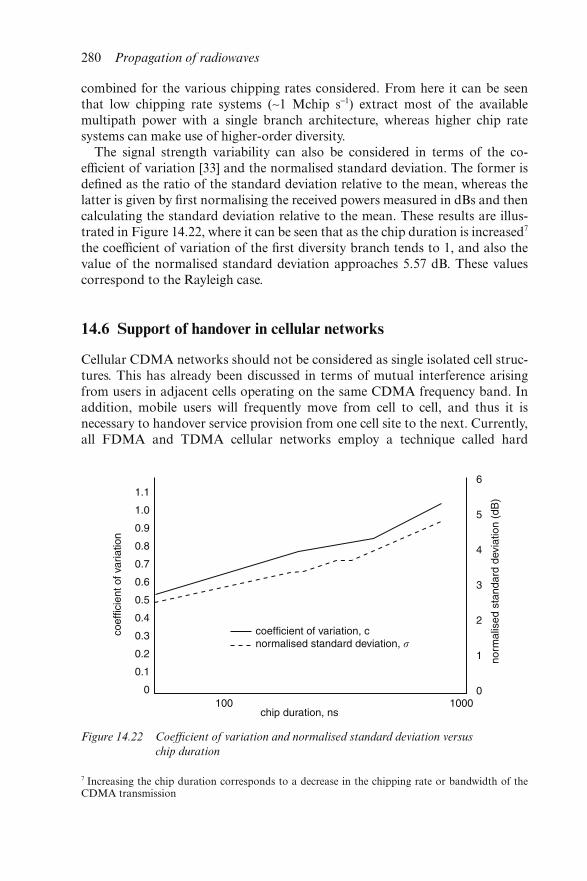
combined for the various chipping rates considered. From here it can be seenthat low chipping rate systems (∼1 Mchip s−1) extract most of the availablemultipath power with a single branch architecture, whereas higher chip ratesystems can make use of higher-order diversity.
The signal strength variability can also be considered in terms of the co-efficient of variation [33] and the normalised standard deviation. The former isdefined as the ratio of the standard deviation relative to the mean, whereas thelatter is given by first normalising the received powers measured in dBs and thencalculating the standard deviation relative to the mean. These results are illus-trated in Figure 14.22, where it can be seen that as the chip duration is increased7
the coefficient of variation of the first diversity branch tends to 1, and also thevalue of the normalised standard deviation approaches 5.57 dB. These valuescorrespond to the Rayleigh case.
14.6 Support of handover in cellular networks
Cellular CDMA networks should not be considered as single isolated cell struc-tures. This has already been discussed in terms of mutual interference arisingfrom users in adjacent cells operating on the same CDMA frequency band. Inaddition, mobile users will frequently move from cell to cell, and thus it isnecessary to handover service provision from one cell site to the next. Currently,all FDMA and TDMA cellular networks employ a technique called hard
Figure 14.22 Coefficient of variation and normalised standard deviation versus
chip duration
7 Increasing the chip duration corresponds to a decrease in the chipping rate or bandwidth of theCDMA transmission
280 Propagation of radiowaves
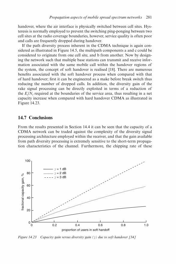
handover, where the air interface is physically switched between cell sites. Hys-teresis is normally employed to prevent the switching ping-ponging between twocell sites at the radio coverage boundaries, however, service quality is often poorand calls are frequently dropped during handover.
If the path diversity process inherent in the CDMA technique is again con-sidered as illustrated in Figure 14.5, the multipath components a and c could beconsidered to originate from one cell site, and b from another. Now by design-ing the network such that multiple base stations can transmit and receive infor-mation associated with the same mobile call within the handover regions ofthe system, the concept of soft handover is realised [18]. There are numerousbenefits associated with the soft handover process when compared with thatof hard handover; first it can be engineered as a make before break switch thusreducing the number of dropped calls. In addition, the diversity gain of therake signal processing can be directly exploited in terms of a reduction ofthe Es/NI required at the boundaries of the service area, thus resulting in a netcapacity increase when compared with hard handover CDMA as illustrated inFigure 14.23.
14.7 Conclusions
From the results presented in Section 14.4 it can be seen that the capacity of aCDMA network can be traded against the complexity of the diversity signalprocessing architecture employed within the receiver, and that the gain availablefrom path diversity processing is extremely sensitive to the short-term propaga-tion characteristics of the channel. Furthermore, the chipping rate of these
Figure 14.23 Capacity gain versus diversity gain (γ) due to soft handover [34]
Propagation aspects of mobile spread spectrum networks 281
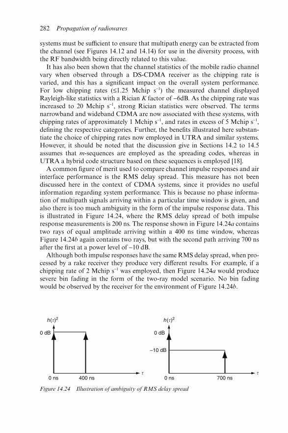
systems must be sufficient to ensure that multipath energy can be extracted fromthe channel (see Figures 14.12 and 14.14) for use in the diversity process, withthe RF bandwidth being directly related to this value.
It has also been shown that the channel statistics of the mobile radio channelvary when observed through a DS-CDMA receiver as the chipping rate isvaried, and this has a significant impact on the overall system performance.For low chipping rates (≤1.25 Mchip s−1) the measured channel displayedRayleigh-like statistics with a Rician K factor of −6dB. As the chipping rate wasincreased to 20 Mchip s−1, strong Rician statistics were observed. The termsnarrowband and wideband CDMA are now associated with these systems, withchipping rates of approximately 1 Mchip s−1, and rates in excess of 5 Mchip s−1,defining the respective categories. Further, the benefits illustrated here substan-tiate the choice of chipping rates now employed in UTRA and similar systems.However, it should be noted that the discussion give in Sections 14.2 to 14.5assumes that m-sequences are employed as the spreading codes, whereas inUTRA a hybrid code structure based on these sequences is employed [18].
A common figure of merit used to compare channel impulse responses and airinterface performance is the RMS delay spread. This measure has not beendiscussed here in the context of CDMA systems, since it provides no usefulinformation regarding system performance. This is because no phase informa-tion of multipath signals arriving within a particular time window is given, andalso there is too much ambiguity in the form of the impulse response data. Thisis illustrated in Figure 14.24, where the RMS delay spread of both impulseresponse measurements is 200 ns. The response shown in Figure 14.24a containstwo rays of equal amplitude arriving within a 400 ns time window, whereasFigure 14.24b again contains two rays, but with the second path arriving 700 nsafter the first at a power level of −10 dB.
Although both impulse responses have the same RMS delay spread, when pro-cessed by a rake receiver they produce very different results. For example, if achipping rate of 2 Mchip s−1 was employed, then Figure 14.24a would producesevere bin fading in the form of the two-ray model scenario. No bin fadingwould be observed by the receiver for the environment of Figure 14.24b.
Figure 14.24 Illustration of ambiguity of RMS delay spread
282 Propagation of radiowaves
14.8 Acknowledgments
The authors wish to express their sincere thanks to colleagues at the Centre forCommunication Research (University of Bristol), in particular to Prof. JoeMcGeehan, Dr. Simon Swales, Dr. Andy Nix and Dr. Joseph Cheung fortheir invaluable help and support of this work. We also greatly value the earlycontributions from Dr. Amnon Hammer on CDMA capacity analysis.
14.9 References
1 RICHARDSON, K.W.: ‘UMTS overview’, Electron. Commun. Eng. J.,2000, 12, 3, pp.93–100
2 BULL, D.R., CANAGARAJAH, C.N. and NIX, N.R.: ‘Insights intomobile multimedia communications’ (Academic Press, 2000)
3 PAJUKOSKI, K. and SAVUSALO, J.: ‘Wideband CDMA test system’.Proceedings of IEEE international conference on Personal indoor andmobile radio communications, PIMRC’97, Helsinki, Finland, 1–4 September1997, pp.667–672
4 ‘CEC, RACE mobile telecommunications workshop’’. DG XIII/B,RA129–93, Metz, France, 16–18 June 1993
5 BEACH, M.A.: ‘A CDMA air interface for mobile access’, ‘Digital mobileradio towards future generation systems’ (COST231 final report), ch. 7.2
6 http://www.3gpp.org7 DIXON, R.C.: ‘Spread spectrum systems’ (John Wiley & Sons, Inc., 1984,
2nd edn.)8 LIVNEH, N. et al.: ‘Frequency hopping CDMA for future cellular radio’.
IEEE 42nd VTC, Denver, May 1992, pp.400–4049 PURLE, D.J. et al.: ‘Investigation of propagation through a frequency
hopped channel’, Electron. Lett., 1992, 29, 9, pp.785–610 http://www.bluetooth.org/11 GILHOUSEN, K.S. et al.: ‘On the capacity of a cellular CDMA system’,
IEEE Trans. Veh. Technol., 1991, 40, pp.303–31212 SCHILLING, D.S.: ‘Broadband CDMA overlay’. IEEE 43rd VTC, New
Jersey, May 1993, pp.452–45513 OMURA, J.K.: ‘Spread spectrum radios for personal communication
services’. IEEE International symposium on Personal, indoor and mobileradio communications, November 1992
14 PARSONS, J.D: ‘The mobile radio propagation channel’ (Wiley, 2000, 2ndedn.)
15 GOLOMB, S.W.: ‘Shift register sequences’ (Aegean Park Press, California,1982, revised edn.)
16 Digital land mobile radio communications, final report. CEC COST207,CD-NA-12160-EN-C, Brussels, 1989
17 YANG, S.C.: CDMA RF system engineering (Artech House, 1998)18 HOLMA, H, and TOSKALA, A.: ‘WCDMA for UMTS’, (Wiley, 2000)19 LEE, W.C.Y.: ‘Overview of cellular CDMA’, IEEE Trans. Vch. Technol.,
1991, 40, pp. 291–310
Propagation aspects of mobile spread spectrum networks 283
20 SIMON, M.K. et al.: ‘Spread spectrum communications’ (ComputerScience Press, Rockville, 1985, vols. I–III)
21 LEE, J.S., & MILLER, L.E.: ‘CDMA systems engineering handbook’(Artech House, 1998)
22 NIKULA, E., TOSKALA, A., DAHLMAN, E., GIRARD, L., andKLEIN, L.: ‘FRAMES multiple access for UMTS and IMT2000’, IEEEPers. Commun., 1998, pp.16–24
23 BEACH, M.A. et al.: ‘An evaluation of direct sequence CDMA for futuremobile personal communication networks’. IEEE VTC, St. Louis, May1991, pp.63–70
24 GILHOUSEN, K.S.: ‘Mobile power control for CDMA’, IEEE Trans.Commun., 1992, pp.34–38
25 WIJAYASURIYA, S.S.H. et al.: ‘Rake Decorrelating Receiver for DS-CDMA mobile radio networks’, Electron. Lett., 1992, 29, pp.395–396
26 HONIG, M., and TSATSANIS, M.K.: ‘Adaptive techniques for multiuserCDMA receivers’, IEEE Signal Process. Mag., 2000, 17, (3), pp.49–61
27 PURSLEY, M.B.: ‘Performance evaluation for phased-coded spread spec-trum multiple access communications – part I: system analysis’, IEEETrans. Commun., 1977, COM-25, pp.795–799
28 ALLPRESS, S.A.: ‘Optimising signalling rate and internal diversity orderfor the mobile cellular DS-CDMA systems’. PhD thesis, University ofBristol, Bristol, December 1993
29 ALLPRESS, S.A. and BEACH, M.A.: ‘Measurement & characterisation ofthe wideband DS-CDMA radio channel’. IEE ICAP93, Edinburgh, March1993, pp.429–432
30 ALLPRESS, S.A. and BEACH, M.A.: ‘On the optimum DS-CDMA chan-nel bandwidth for personal communication systems’. IEEE 43rd VTC, NewJersey, May 1993, pp.436–439
31 COX, D.C., and LECK, R.P.: ‘Correlation bandwidth and delay spreadmultipath propagation statistics for 910 MHz urban mobile radio channels’,IEEE Trans. on Commun., 1985, 23, pp.1275–1280
32 HOLTZMAN, J.M. and JALLOUL, L.M.A.: ‘Rayleigh fading effect reduc-tion with wideband DS-CDMA signals’. Technical Report, RutgersUniversity, August 1991
33 MILLER, I. and FREUD, J.: ‘Probability and statistics for engineers’,(Prentice-Hall, 1985, 3rd edn. 1985)
34 CHEUNG, J.C.S. et al.: ‘On the impact of soft handoff on cellular directsequence code division multiple access system’. CEC RACE PLATON/UOB/037/WPD2/07/ 93/Issue1, July 1993
284 Propagation of radiowaves
Chapter 15
Basic physics of the ionosphere
H. Rishbeth
15.1 Introduction
15.1.1 What is the ionosphere?
The ionosphere is the part of the atmosphere in which free electrons are suf-ficiently numerous to influence the propagation of radiowaves. Very roughly, itextends in height from 70 to 600 km, although its upper limit is not well defined.In ionospheric parlance the term region (D, E, F) denotes parts of the atmo-sphere, the D/E boundary being conventionally at 90 km height and the E/Fboundary at 150 km. The term layer refers to ionisation within a region, such asthe F1 and F2 layers in the F region and the E, E2 and sporadic E layers in theE region (Figure 15.1).
The term plasma is used for an ionised gas; the ionosphere is a weak plasmabecause, even in the F region by day, no more than one part in 106 of the gas isionised. The ionosphere is electrically neutral to a high degree of approximation,as positive and negative charged particles are always created and destroyedtogether.
15.1.2 Where does the ionosphere fit into the atmosphere?
Figure 1.2 of Chapter 1 shows the main regions of the neutral atmosphere: thetroposphere (0–12 km), where the temperature decreases upwards; stratosphere(12–30 km), a turbulent region of fairly uniform temperature; mesosphere(30–80 km), heated by absorption of solar UV radiation by ozone; and thethermosphere above 80 km, strongly heated by solar extreme ultraviolet (EUV)and X-rays. In the thermosphere, the temperature increases rapidly upwardstowards the limiting exospheric temperature, which on average is about 1000 K.In the exosphere, above about 600 km, individual atoms move freely in satellite-like orbits controlled by the earth’s gravity. The solar EUV and X-rays dissociate
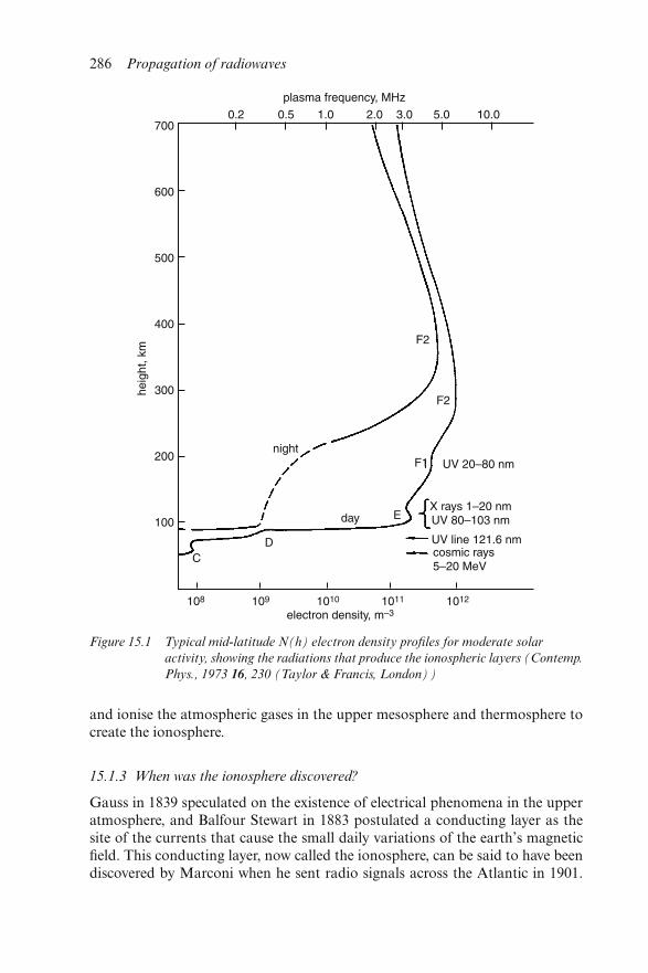
and ionise the atmospheric gases in the upper mesosphere and thermosphere tocreate the ionosphere.
15.1.3 When was the ionosphere discovered?
Gauss in 1839 speculated on the existence of electrical phenomena in the upperatmosphere, and Balfour Stewart in 1883 postulated a conducting layer as thesite of the currents that cause the small daily variations of the earth’s magneticfield. This conducting layer, now called the ionosphere, can be said to have beendiscovered by Marconi when he sent radio signals across the Atlantic in 1901.
Figure 15.1 Typical mid-latitude N(h) electron density profiles for moderate solar
activity, showing the radiations that produce the ionospheric layers (Contemp.
Phys., 1973 16, 230 (Taylor & Francis, London))
286 Propagation of radiowaves
Lodge in 1902 correctly surmised that it contains free electrons and ions pro-duced by solar ionising radiation. Research really began in 1924 when Appletonand Barnett and Breit and Tuve measured the height of the reflecting layers.
15.1.4 How do we study the ionosphere?
Ground-based techniques sound the ionosphere with radiowaves, which arereturned from the ionosphere in three ways: by total reflection (ionosondes); bypartial reflection or coherent scatter from small-scale structures in the iono-sphere; or by incoherent scatter from the ion and electrons. These techniques areclassed as radar; there is a historical link between the invention of radar andionospheric research. Rockets and satellites enable in situ measurements andspace/ground radio propagation experiments. See Table 15.1.
15.1.5 Why do we study the ionosphere?
The ionosphere is important because of its role in radiocommunications, andalso scientifically because the electrons are easier to detect experimentally thanthe neutral air and thus act as tracers for studying the upper atmosphere. Theelectrons and ions form a weakly ionised gas or plasma, and the plasma physicsassociated with detailed ionospheric structure is relevant to radio propagation.Other current research topics are prediction and forecasting of ionospheric con-ditions on various time scales (space weather) and long-term studies of globalchange.
15.1.6 What are the most important characteristics of the ionosphere?
For radio propagation, the most important ionospheric characteristics are thecritical frequencies (penetration frequencies at vertical incidence) for the ordin-ary magnetoionic mode (the extraordinary critical frequencies, which existbecause of the birefringence caused by the Earth’s magnetic field, are lessimportant). For any layer the ordinary critical frequency is related to the peakelectron density (electron concentration) Nm by:
f0 = 80.6 Nm or f0 ≈ 9√Nm (15.1)
in which the MKS numerical factors are derived from physical constants. Otherimportant characteristics are the heights hm of the peaks of the layers, and thetotal or height-integrated electron content of the whole ionosphere.
15.2 The environment of the ionosphere
15.2.1 Ionising solar radiations
The sun emits radiations in the X-ray and extreme ultraviolet (EUV) parts ofthe electromagnetic spectrum, which comprise spectral lines and a background
Basic physics of the ionosphere 287
of continuum radiation. The sun also emits energetic particles, but most of thesehave insufficient energy to ionise the atmosphere.
Sunspots themselves do not influence the ionosphere, but the strength ofmany solar emissions that do influence the ionosphere are linked to the sunspotnumber, a standard index of solar activity that rises and falls with the 11-yearsolar cycle; its values go back to 1749. Since 1948, the radio flux density of thesun at 10.7 cm wavelength has been routinely measured, as it also is found to bea good indicator of the ionising radiation (although the radio emission itself hasno geophysical consequences).
Any particular radiation (wavelength λ) ionises gases for which the ionisation
Table 15.1 Experimental techniques for studying the ionosphere
Radio probing• Total reflection at plasma frequency fp = √(80.6 N) (typically HF/MF/LF in
daytime F/E/D layers respectively). Used for routine sounding byionosondes (which produce records known as ionograms). Cannot observeabove F2 peak, except by topside sounders carried in satellites. Reflection isinfluenced by the geomagnetic field.
• Coherent scatter at frequencies >> fp (HF, VHF, UHF). Scattering fromirregularities of scale size λ/2 (λ = radar wavelength), which occur in the auroraloval and near the magnetic equator; also from meteor trails. Measures velocityby Doppler effect.
• Incoherent scatter at frequencies >> fp (VHF, UHF). Thomson scattering fromthermal random irregularities (ion-acoustic waves) of scale size λ/2. Very weak(depends on electron cross section, 10−28 m2; the total target area is ∼1 mm2).Measures ion density, ion and electron temperatures, ion drift velocity, andindirectly some neutral atmosphere parameters.
Active remote sensing (using man-made signals traversing ionosphere)• radio phase and polarisation (Faraday rotation)• LF, VLF reflection, MF partial reflection in lower ionosphere• radiowave absorption (signal strength)• radar studies of meteor echoes (neutral winds, density)
Passive remote sensing from ground or space (using natural emissions); thesetechniques suffer from lack of height discrimination• absorption of cosmic radiowaves; radio star refraction• aurora – interferometry and imaging• airglow – temperature and velocity of emitting gases
In situ measurements (using instruments on rockets and satellites); good space andtime resolution but no systematic coverage• density, composition, temperature, velocity of ionised and neutral gas• electric and magnetic fields• tracking of objects and chemical trails released from spacecraft• analysis of satellite orbits (giving air density)
Active experiments (e.g. r.f. heating, release of active chemicals)
288 Propagation of radiowaves
limit (79.6 nm for N2, 91.1 nm for O and H, 102.7 nm for O2 and 134 nm for NO)is longer than λ; the height to which the radiation penetrates depends on itsabsorption cross section σ (see section 15.3.1). The ionosphere is layered becauseσ is different for different radiations, the sources of the layers shown in Figure15.1 being as follows (with some important lines indicated):
F1 layer (150–180 km): EUV 20–80 nm (He II 30.4 nm, He I 58.4 nm)E layer (100–120 km): X-rays 1–20 nm, EUV 80–103 nm (Lyβ 102.6 nm)D layer (70–90 km): Lyα 121.6 nm, X-rays 0.1–1 nmC layer (50–70 km, an insignificant layer): MeV cosmic rays
No photon radiation has a large enough σ to be strongly absorbed at the heightof the F2 layer; this layer is produced by the same band of radiation thatproduces the F1 layer. The electron density is greater in the F2 layer than in theF1 layer because of the smaller electron loss (Section 15.3.4). Charged particlescan also ionise, at a height which depends on their energy.
15.2.2 Temperature at ionospheric heights
The ionospheric layers lie within the thermosphere, where the temperature T
varies with height h. At the base, T is governed by the mesopause temperature,usually 150–180 K, but it increases rapidly upwards with a gradient dT/dh
determined by the solar heat input. Higher up, the thermal conductivity ofthe air becomes large and the temperature gradient flattens out. Above about300 km, the temperature tends to a limit known as the exospheric temperatureT∞ which varies considerably with local time (LT), latitude, season and the11-year sunspot cycle. The temperature variations are mainly due to solarheating, which causes the atmosphere to expand on the daylit side of the earth,creating a high-pressure region sometimes called the daytime bulge. Typically atmid-latitudes T∞ is 800 K at midday and 600 K at midnight at sunspot minimum,and 1400 K and 1100 K, respectively, at sunspot maximum.
From observations of satellite orbits, which yield extensive data on air density,it is deduced that T∞ is highest around 1400 local time (LT) and lowest around0300 LT; the maxima and minima are in low latitudes near equinox but migrateseasonally, as shown for example in Figure 15.2 which is a simplified map of T∞
at the June solstice. Not shown in the Figure is the localised heating in theauroral ovals (Sections 15.2.5, 15.5.7), which is due to the energy deposited byenergetic particles and electric currents from the magnetosphere.
15.2.3 Composition of the upper atmosphere
The formation of ionospheric layers depends on the density and composition ofthe ambient neutral air. From the ground up to 100 km, the major gases N2 andO2 (mean molar masses M of 28 and 32) are well mixed by winds and turbulencewith a concentration ratio of about 4:1, giving a mean molar mass of about 29.The distributions of minor constituents H2O, CO2, NO and O3 are controlled by
Basic physics of the ionosphere 289
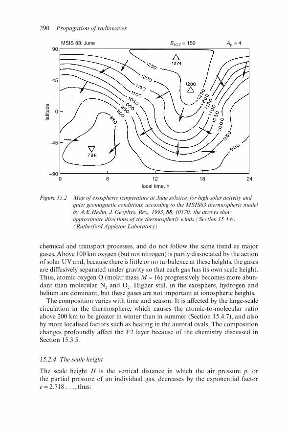
chemical and transport processes, and do not follow the same trend as majorgases. Above 100 km oxygen (but not nitrogen) is partly dissociated by the actionof solar UV and, because there is little or no turbulence at these heights, the gasesare diffusively separated under gravity so that each gas has its own scale height.Thus, atomic oxygen O (molar mass M = 16) progressively becomes more abun-dant than molecular N2 and O2. Higher still, in the exosphere, hydrogen andhelium are dominant, but these gases are not important at ionospheric heights.
The composition varies with time and season. It is affected by the large-scalecirculation in the thermosphere, which causes the atomic-to-molecular ratioabove 200 km to be greater in winter than in summer (Section 15.4.7), and alsoby more localised factors such as heating in the auroral ovals. The compositionchanges profoundly affect the F2 layer because of the chemistry discussed inSection 15.3.5.
15.2.4 The scale height
The scale height H is the vertical distance in which the air pressure p, orthe partial pressure of an individual gas, decreases by the exponential factore = 2.718 . . ., thus:
Figure 15.2 Map of exospheric temperature at June solstice, for high solar activity and
quiet geomagnetic conditions, according to the MSIS83 thermospheric model
by A.E.Hedin, J. Geophys. Res., 1993, 88, 10170; the arrows show
approximate directions of the thermospheric winds (Section 15.4.6)
(Rutherford Appleton Laboratory)
290 Propagation of radiowaves
(1/H) = −d(ln p)/dh (15.2)
The scale height may be deduced from the hydrostatic or barometric Eqn. 15.3 inwhich the vertical pressure gradient is balanced against gravity:
−dp/dh = ρg = nmg (15.3)
where h = height, ρ = density, n = concentration, g = acceleration due to gravity,m = particle mass (in kg, as compared to M which is the molar mass in atomicmass units). Using the perfect gas law in either of two forms:
p = nkT = ρRT/M (15.4)
where k = Boltzmann’s constant, R = gas constant and T = temperature, toeliminate the density ρ, the scale height is found to be (again in either of twoforms):
H = kT/mg = RT/Mg (15.5)
H may be defined either for a single gas or for the air as a whole (in which case Mis averaged over all the gases present). Integrating Eqn. 15.2 with respect toheight gives the variation of pressure above any chosen base level h0, at which p =p0, viz.:
p = p0 e−z ∼ p0 exp ( (h0 − h)/H) (15.6)
where
z = ∫ (dh/H) ∼ (h0 − h)/H (15.7)
is known as the reduced height, and is measured in units of H above the baselevel h0. In Eqns. 15.6 and 15.7 the simplified expressions that follow the symbol ∼apply if H is constant with height – which is not really the case in the thermo-sphere, because T increases upwards and M decreases upwards, while g
decreases upwards by about three per cent per 100 km. Whether or not H varieswith height, it is easily shown that the total number of particles in a verticalcolumn above any height h0 is Hn(h0), so H may be regarded as the thickness ofthe atmosphere.
15.2.5 The geomagnetic field
The earth’s magnetic field plays an important role in the ionosphere, because itlargely governs the motions of ionospheric ions and electrons. It may beapproximated by a dipole inclined at 12° to the earth’s axis, slightly offset fromthe earth’s centre in the direction of the Pacific Ocean. In low and middlelatitudes the geomagnetic field lines are closed, but at higher latitudes they arelinked to the magnetosphere, the tenuous region around the earth that is perme-ated by the geomagnetic field. The small daily variations of the geomagneticfield (of the order of 0.1 per cent) are produced by currents flowing in the iono-sphere, generated by dynamo action of winds blowing across the geomagneticfield lines (Section 15.4.3).
Basic physics of the ionosphere 291
The high latitude ionosphere is profoundly affected by charged particles andelectric currents, originating in the magnetosphere, which cause the aurora andmagnetic storms. The particles and currents mainly enter the atmosphere in theauroral ovals, rings 2000–3000 km in diameter that surround the magnetic poles(Section 15.5.7). In turn the magnetosphere is influenced by the stream ofcharged particles emitted by the sun (the solar wind) and the interplanetarymagnetic field.
Magnetic storms tend to follow solar disturbances and the resulting strength-ening of the solar wind (Section 15.6.2). During storms, the electric currents inthe high latitude ionosphere may locally perturb the geomagnetic field by up tofive per cent. The degree of geomagnetic disturbance is characterised by planet-ary geomagnetic indices (Ap and Kp), which are computed for every three hoursof universal time from records made at several magnetic observatories.
15.3 Formation and photochemistry of the ionised layers
15.3.1 The Chapman formula for production of ionisation
The simple Chapman theory of the production of an ionised layer starts byassuming (a) monochromatic solar radiation acting on (b) a plane atmospherecontaining (c) a single ionisable gas with (d) a constant scale height. All foursimplifications (a–d) can be removed, but the equations then become morecomplicated.
Figure 15.3 shows the principles of the theory. Ionising radiation, initially ofintensity I∞, strikes the top of the atmosphere at zenith angle (obliquity) χ, andits intensity I(h) decreases as it travels downwards, according to the equation:
dI/I = −σn dh sec χ = −dτ (15.8)
where σ is the absorption cross section and τ is optical depth. By integratingEqn. 15.8 along the path of the radiation, from the top of the atmosphere downto height h, and using the property that ∫ n dh = n(h).H (as mentioned in Section15.2.2), it is found that:
I(h) = I∞ exp(−nσH sec χ) = I∞ exp (− τ(h) ) (15.9)
From Eqn. 15.9 it may be seen that, for oblique sun, attenuation begins at ahigher height (as shown by dots in Figure 15.3) than for overhead sun. Theproduction rate q is found by multiplying the intensity of the radiation (dashedcurve) by the gas concentration n (continuous curve) and by the cross section σand ionising efficiency η. Thus:
q(h) = I(h) ησn(h) = I∞ ησn(h) exp (− τ(h) ) (15.10)
On differentiating Eqn. 15.10, it is found that the peak value of q occurs at theheight where τ = 1 (unit optical depth). The height of peak production is givenby:
292 Propagation of radiowaves
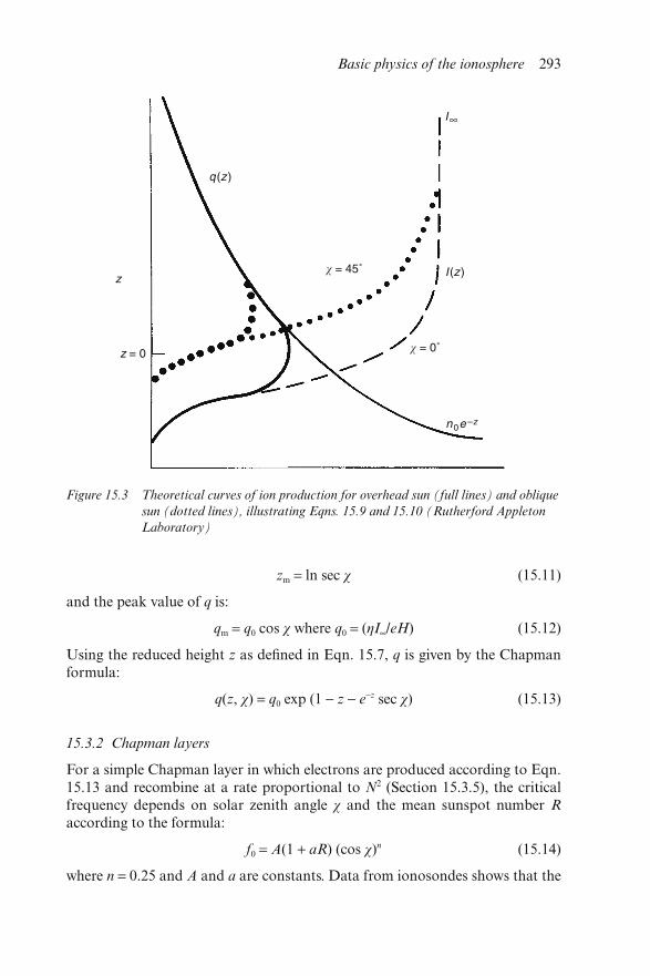
zm = ln sec χ (15.11)
and the peak value of q is:
qm = q0 cos χ where q0 = (ηI∞/eH) (15.12)
Using the reduced height z as defined in Eqn. 15.7, q is given by the Chapmanformula:
q(z, χ) = q0 exp (1 − z − e−z sec χ) (15.13)
15.3.2 Chapman layers
For a simple Chapman layer in which electrons are produced according to Eqn.15.13 and recombine at a rate proportional to N2 (Section 15.3.5), the criticalfrequency depends on solar zenith angle χ and the mean sunspot number R
according to the formula:
f0 = A(1 + aR) (cos χ)n (15.14)
where n = 0.25 and A and a are constants. Data from ionosondes shows that the
Figure 15.3 Theoretical curves of ion production for overhead sun (full lines) and oblique
sun (dotted lines), illustrating Eqns. 15.9 and 15.10 (Rutherford Appleton
Laboratory)
Basic physics of the ionosphere 293
daytime E and F1 layers follow this formula quite well when χ varies with timeof day, season, and latitude, although the index n actually varies between about0.2 and 0.35. The incident solar flux I∞ varies with the solar cycle and so f0 variesregularly with the sunspot number. Figure 15.4 shows the regular seasonal andsolar cycle variations of the E and F1 layers at Slough and Port Stanley, togetherwith solar and interplanetary parameters. The normal D layer (although notpossessing a measurable critical frequency) also varies quite regularly with cos χ.The F2 layer does not: careful examination of the seasonal ripple of Slough f0
F2 shows that it is out of phase with those of f0F1 and f0E, which do conform tothe variation of cos χ. At Port Stanley, however, the F2 layer has a predomin-antly semiannual variation, with maxima at the equinoxes.
15.3.3 The continuity equation
The electron density in the ionosphere is subject to the basic physical principlesof conservation of mass, momentum and energy which, respectively, areexpressed mathematically by the continuity equation for the electron density, theequation of motion for the electrons and ions, and equations expressing the heatbalance (which is not discussed here). These equations may be formulated forany charged or neutral constituent of the atmosphere. Equations of motion areconsidered in Section 15.4.1. The present section deals with the continuityequation for the electrons and ions (the ionised plasma), which is:
∂N/∂t = q − L(N) − div (NV) (15.15)
The loss term L(N) can generally be simplified as follows:
E & F1 layers: L(N) = αN2
F2 layer: L(N) = βN(15.16)
where α, β are the square-law and linear loss coefficients (Section 15.3.5). Thetransport term, in which V is the plasma drift velocity, the drift velocity of theionisation, is often simplified by omitting horizontal motion, which usually con-tributes little to div (NV), and including only the vertical drift velocity, W, inwhich case:
div (NV) = ∂(NW)/∂h (15.17)
15.3.4 Ion chemistry
Reactions in the ionosphere have to conserve energy and momentum, besidessatisfying the principles of quantum theory. One consequence is that atomic ionscannot recombine easily with electrons, unless a third body takes part in thereaction and absorbs the excess energy. This requires a three-body collision,which is only likely to occur below 100 km where the air density is sufficientlyhigh. Molecular ions, however, recombine easily at any height, since theycan dissociate to give two products as in Eqns. 15.24–15.26. Throughout the
294 Propagation of radiowaves
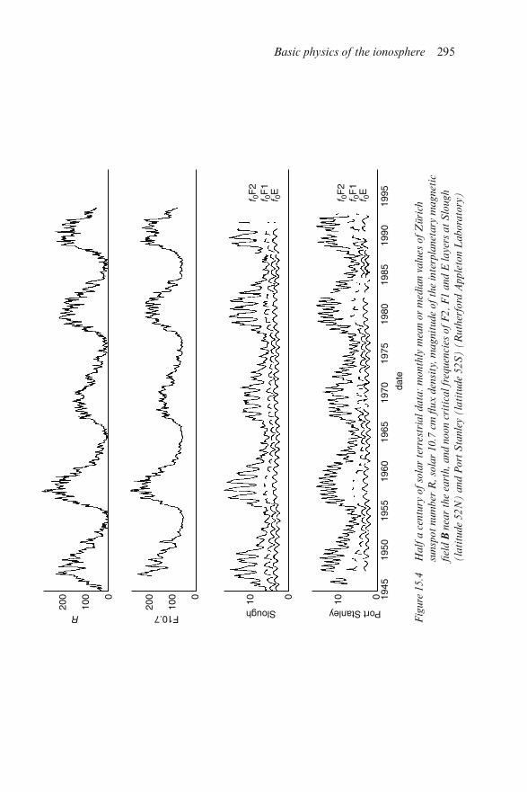
Fig
ure
15.4
Half
a c
entu
ry o
f so
lar
terr
estr
ial
data
: m
onth
ly m
ean o
r m
edia
n v
alu
es o
f Z
üri
ch
sunsp
ot
num
ber
R,
sola
r 10.7
cm
flux
den
sity
, m
agnit
ude
of
the
inte
rpla
net
ary
magnet
ic
fiel
d B
nea
r th
e ea
rth,
and n
oon c
riti
cal
freq
uen
cies
of
F2,
F1 a
nd E
layer
s at
Slo
ugh
(la
titu
de
52N
) a
nd P
ort
Sta
nle
y (
lati
tude
52S
) (
Ruth
erfo
rd A
pple
ton L
abora
tory
)
Basic physics of the ionosphere 295
ionosphere, reactions may leave atoms and molecules in excited states, whichsubsequently decay by emitting radiation. This is the origin of the upperatmosphere luminescence, the airglow.
In the D region, the atmosphere is relatively dense, so both two-body andthree-body collisions occur and complicated chemical reactions take place.Electrons may become attached to atoms or molecules to form negative ions.Negative ions are more abundant than electrons at all heights below 90 km atnight but, being destroyed by visible and ultraviolet sunlight, they are onlyabundant below 70 km by day. Many ions, both positive and negative, becomeattached to water molecules to form complex clusters.
In the E region, the atmosphere is more rarefied and only two-body collisionsoccur, so atomic ions cannot recombine easily with electrons, but are readilyconverted to molecular ions by reactions such as Eqns 15.21–15.23. The overallresult is that the positive ions are mostly molecular, NO− and O2
+, and the losscoefficient α is of the square-law type in Eqn. 15.16. Some metal atoms (Fe+,Mg+, Ca+), traces of which are deposited in the atmosphere by meteors, becomeionised to produce long-lived metallic ions that are the main ionic component ofmid-latitude sporadic E layers (Section 15.5.3). At greater heights, in the Fregion, the ions are mainly NO+ and O2
+ (F1 layer) and O+ (F2 layer), asdescribed in the following simplified summary of the chemistry.
15.3.5 The photochemical scheme of the ionosphere
Up to the F2 peak, the distribution of ions and electrons is essentially deter-mined by photochemical processes of production and loss. As described in Sec-tion 15.2.1, the major gases in the thermosphere are ionised by EUV photons(hν), giving O+, N2
+ and some O2+ ions, plus electrons. For example:
O + hν → O+ + e− (15.18)
N2 + hν → N2+ + e− (15.19)
O2 + hν → O2+ + e− (15.20)
Ions collide with neutral molecules and undergo charge transfer or chargeexchange reactions which produce molecular ions, for example:
O+ + O2 → O2+ + O (15.21)
O+ + N2 → NO+ + N (15.22)
N2+ + O → NO+ + N (15.23)
Molecular ions recombine with electrons and dissociate thus:
NO+ + e− → N + O (15.24)
O2+ + e− → O + O (15.25)
N2+ + e− → N + N (15.26)
296 Propagation of radiowaves
This photochemical scheme has several consequences; the experimental evi-dence for (a)–(d) comes mainly from observations made by rocket-borne andsatellite-borne instruments, such as mass spectrometers, and for (e)–(h) from theelectron distributions measured by ionosondes:
(a) Despite the abundance of neutral N2, very few N2+ ions are present, as they
are rapidly destroyed via reaction 15.23 as well as by reaction 15.24.(b) NO+ ions are abundant because they are rapidly formed via reactions 15.22
and 15.23, even though neutral NO is hardly present at all.(c) Below about 200 km molecular ions dominate, because the O+ ions are
rapidly converted to O2+ and NO+ via reactions 15.21 and 15.22 by the
relatively abundant O2 and N2.(d) Above about 200 km, reactions 15.21 and 15.22 proceed very slowly
because of the scarcity of N2 and O2 at these heights. Once formed, how-ever, the NO+ and O2
+ ions rapidly recombine with electrons via reactions15.24 and 15.25. As a result, O+ is the dominant ion.
(e) In the E and F1 layers where NO+ and O2+ ions dominate, the loss term in
eqn. 15.15 takes the form aN2, as in Eqn. 15.16.(f) In the F2 layer, the loss term takes the form βN as in Eqn. 15.16, where
β = k′n[O2] + k″n[N2] (15.27)
where k′, k″ are the rate coefficients of reactions 15.21 and 15.22.(g) The F1 layer is the transition between (e) and (f). It is a distinct feature with
its own critical frequency at certain times (mainly summer and at sunspotminimum) but not at other times (especially winter). Its appearance isfound to depend on the relative values of q, α and β.
(h) Above the F1 layer, the electron density increases upwards, because the losscoefficient β (which depends on the N2 and O2 concentrations) decreasesupwards faster than the production rate q (which depends on the O concen-tration). The increase ends at the F2 peak (Section 15.4.8).
This photochemical scheme accounts for the general form of the N(h) profiles asshown in Figure 15.5, up to the F2 peak which is discussed in Section 15.4.7,together with the sketches on the right of the Figure.
15.4 Dynamics of the ionosphere
15.4.1 Equation of motion of the charged particles
To understand the transport processes which determine the transport term inthe continuity equation 15.15, one needs to understand how the ions and elec-trons move under the influence of the forces acting on them, namely gravity g,electrostatic field E, the geomagnetic field B, collisions with the neutral air(which moves with the wind velocity U) and gradients in their own partialpressures pi and pe (thus regarding them as an ion-electron gas or plasma). The
Basic physics of the ionosphere 297
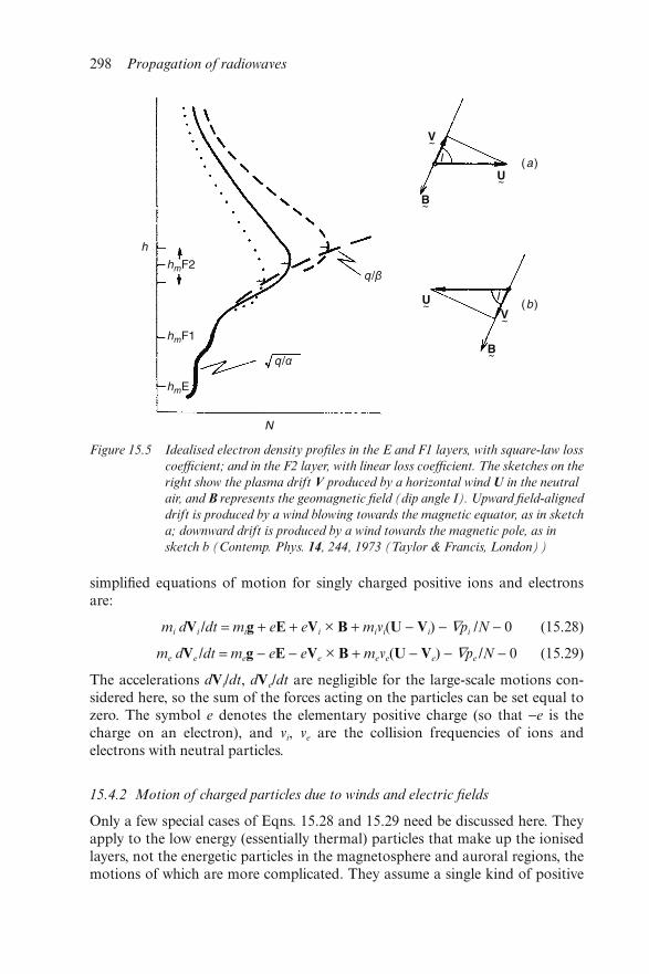
simplified equations of motion for singly charged positive ions and electronsare:
mi dVi /dt = mig + eE + eVi × B + mivi(U − Vi) − ∇pi /N − 0 (15.28)
me dVe /dt = meg − eE − eVe × B + meve(U − Ve) − ∇pe /N − 0 (15.29)
The accelerations dVi/dt, dVe/dt are negligible for the large-scale motions con-sidered here, so the sum of the forces acting on the particles can be set equal tozero. The symbol e denotes the elementary positive charge (so that −e is thecharge on an electron), and vi, ve are the collision frequencies of ions andelectrons with neutral particles.
15.4.2 Motion of charged particles due to winds and electric fields
Only a few special cases of Eqns. 15.28 and 15.29 need be discussed here. Theyapply to the low energy (essentially thermal) particles that make up the ionisedlayers, not the energetic particles in the magnetosphere and auroral regions, themotions of which are more complicated. They assume a single kind of positive
Figure 15.5 Idealised electron density profiles in the E and F1 layers, with square-law loss
coefficient; and in the F2 layer, with linear loss coefficient. The sketches on the
right show the plasma drift V produced by a horizontal wind U in the neutral
air, and B represents the geomagnetic field (dip angle I). Upward field-aligned
drift is produced by a wind blowing towards the magnetic equator, as in sketch
a; downward drift is produced by a wind towards the magnetic pole, as in
sketch b (Contemp. Phys. 14, 244, 1973 (Taylor & Francis, London))
298 Propagation of radiowaves
ion and ignore negative ions (but can easily be generalized to remove theserestrictions). Deleting the acceleration, gravitational and pressure gradientterms, Eqns. 15.28 and 15.29 can be solved to give the following conclusions.
For motion parallel to B: if the neutral air wind has a component parallel toB, it moves both ions and electrons freely in that direction. If the electric fieldhas a component parallel to B, it drives electrons and ions in opposite directions,i.e. there is a high electrical conductivity.
For motion perpendicular to B, the direction of motion depends on the ratioof the collision frequency v (with neutral particles) to the magnetic gyrofre-quency ω = Be/m. Since v decreases exponentially upwards, while ω is almostconstant, the ratio v/ω falls off rapidly with height; it is different for ions andelectrons. The important cases are:
(i) v >> ω (up to 100 km for ions, 60 km for electrons). A wind drives the ionsand electrons at its own speed, U, and the magnetic field has no effect. Anelectric field moves ions parallel and electrons antiparallel to itself, butonly slowly because of the high collision frequency, and the conductivity islow.
(ii) v ∼ ω (at about 125 km for ions, 75 km for electrons). A wind or an electricfield drive ions and electrons in directions inclined to the applied force. Theangle is given by arc tan (v/ω), and is thus 45° at the level where v = ω.
(iii) v << ω (above 150 km for ions, 90 km for electrons). The particles move at90° to the applied force. An electric field moves both ions and electrons atspeed E/B in the same direction; this is the electromagnetic drift velocity(Hall drift), written vectorially as E × B/B2. Since electrons and ions moveat almost exactly the same velocity, there is virtually no current. A neutralair wind U produces practically no motion of ions and electrons across themagnetic field.
Electric currents can flow at heights between 60 and 150 km, where the positiveions and electrons move in different directions because their ratios v/ω are differ-ent. Very little curent flows below 100 km, however, because the electron densityN is usually so small. The current density is given by Ohm’s law for theionosphere which can be expressed in two equivalent ways:
j = Ne(Vi − Ve) = σ . E (15.30)
Eqn. 15.30 shows that the conductivity σ (a tensor quantity because j and E areusually not parallel) depends on the difference between the ion and electronvelocities, as well as on N.
15.4.3 The ionospheric dynamo
The charge separation resulting from the different ion and electron motions isthe basis of the ionospheric dynamo, which is driven by tidal winds (Section15.4.4). The dynamo action was envisaged by Balfour Stuart in 1883, before itsphysical nature was known. The dynamo produces the ionospheric currents that
Basic physics of the ionosphere 299
cause the small daily variations in the geomagnetic field, first detected in the18th century. Most of the dynamo current flows in the E layer where the con-ductivity σ is greatest. At night, the E layer current is very weak because N issmall, although some current flows in the F layer. The electric field that arisesfrom the charge separation causes drift motions of ions and electrons in the Eand F layers, which contribute to the transport term in the continuity equation15.15. Additional currents enter and leave the ionosphere in the auroral oval(Section 15.5.7), flowing along the lines of force of the earth’s magnetic field.They are generated by processes that lead to charge separation in themagnetosphere.
For complicated geometrical reasons, charge separation in the ionosphere isparticularly strong near the magnetic equator where a strong polarisation fielddevelops in the E layer. It has the effect of creating high electric conductivity inthe east–west direction, giving rise to a strong east–west electrojet current. Theequatorial electrojet flows in a narrow belt extending about three degrees eitherside of the dip equator.
In addition to the wind-driven dynamo fields and currents in the ionosphere,electric fields and currents are generated in the magnetosphere and transmittedalong geomagnetic field lines to the high latitude ionosphere and the auroralovals, and spread to some extent to lower latitudes. They cause the strong local-ised east–west currents known as the auroral electrojets which, especially duringmagnetic storms, are major sources of heating at high latitudes mentioned inSection 15.2.2.
15.4.4 Atmospheric tides
Atmospheric tides form a complex system containing many components. Theyare forced (driven) by the heating effect of the sun or the gravitational attractionof the sun and moon. Unlike the case of marine tides (dominated by the moon’sgravitational attraction) the atmospheric tidal motions are forced in three mainways: (1) the absorption of solar EUV and X-rays in the thermosphere; (2) theabsorption of solar UV in the ozone layer; (3) the heating of the ground andlower atmosphere by solar visible and infra-red radiation. The tidal motionsinclude diurnal (24-hour), semidiurnal (12-hour) and other components, plus aweak lunar gravitational (12.4-hour) component. The global winds described inSection 15.4.6 can be regarded as being a special type of diurnal tide.
15.4.5 Atmospheric waves
The upper atmosphere contains many kinds of wave. Besides the tides just men-tioned, they include planetary waves (periods of days); gravity waves (period >5 min); acoustic or compressional waves (period < 4 min); and infrasonicwaves (periods < 1 s), some associated with aurora or with seismic activity.
Gravity waves are oscillations controlled by the buoyancy of the air, i.e. bygravity, and have a minimum period of about five minutes (the Brunt–Väisälä
300 Propagation of radiowaves
period) in the thermosphere. Unlike ocean waves which are virtually confined tothe surface, gravity waves permeate the whole upper atmosphere. They have acomplicated phase structure and, in addition to horizontal propagation, thephase velocity has a downward component which gives the appearance of adownward travelling wave on ionograms, although the group velocity andenergy propagation is inclined slightly upwards.
Short and medium period gravity waves (5–30 min) are generated in the loweratmosphere by storms, by winds blowing over mountains and occasionally byman-made explosions. Long period gravity waves (periods 0.5–3 hours) origin-ate from disturbances in the auroral oval; they often travel for thousands ofkilometres, and are prevalent at times of geomagnetic disturbance. Such large-scale waves can have some effect on radio propagation, even at frequencies farabove the ionospheric critical frequencies.
15.4.6 Thermospheric winds
The thermosphere is a vast heat engine driven by solar, magnetospheric andinterplanetary sources, which produce the global temperature variations shownin Figure 15.2; these give rise to horizontal pressure gradients that drive winds inthe directions shown by the arrows. The winds form a global circulation whichcarries heat away from the source regions and liberates it elsewhere. The velocityU is controlled by the Coriolis force due to the earth’s rotation with angularvelocity Ω, by the molecular viscosity of the air (coefficient μ), and by ion drag,the friction due to collisions between air molecules and ions. Ion drag existsbecause the ions are constrained by the geomagnetic field and cannot movefreely with the wind (although they may be driven across the geomagnetic fieldby electric fields, Section 15.4.2). The equation of motion for the horizontalwind is:
dU/dt = F − 2 Ω × U − KN(U − V) − (μ/ρ) ∇ 2U (15.31)
where F is the driving force due to the horizontal pressure gradients ∂p/∂x, ∂p/∂y.Its zonal (west-to-east) and meridional (south-to-north) components are,respectively:
Fx = −(1/ρ) ∂p/∂x, Fy = −(1/ρ) ∂p/∂y (15.32)
The vertical component of F is omitted, as it almost exactly balanced bygravity as in the hydrostatic equation, Eqn. 15.3. The product KN is the ion-neutral collision frequency. At great heights (small ρ) the kinematic viscosity(μ/ρ) is large and viscosity tends to smooth out any wind shears (variations ofwind velocity with height).
Unlike winds in the lower atmosphere, thermospheric winds are described bythe direction towards which they blow. Their direction depends on the ratio ofCoriolis force to ion drag. Two limiting cases are:
U = F/(2 Ω sin φ) (15.33)
Basic physics of the ionosphere 301
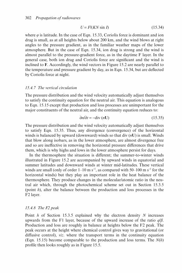
U = F/(KN sin I) (15.34)
where φ is latitude. In the case of Eqn. 15.33, Coriolis force is dominant and iondrag is small, as at all heights below about 200 km, and the wind blows at rightangles to the pressure gradient, as in the familiar weather maps of the loweratmosphere. But in the case of Eqn. 15.34, ion drag is strong and the wind isalmost parallel to the pressure-gradient force, as in the daytime F layer. In thegeneral case, both ion drag and Coriolis force are significant and the wind isinclined to F. Accordingly, the wind vectors in Figure 15.2 are nearly parallel tothe temperature and pressure gradient by day, as in Eqn. 15.34, but are deflectedby Coriolis force at night.
15.4.7 The vertical circulation
The pressure distribution and the wind velocity automatically adjust themselvesto satisfy the continuity equation for the neutral air. This equation is analogousto Eqn. 15.15 except that production and loss processes are unimportant for themajor constituents of the neutral air, and the continuity equation reduces to:
∂n/∂t = −div (nU) (15.35)
The pressure distribution and the wind velocity automatically adjust themselvesto satisfy Eqn. 15.35. Thus, any divergence (convergence) of the horizontalwinds is balanced by upward (downward) winds so that div (nU) is small. Windsthat blow along isobars, as in the lower atmosphere, are almost divergence freeand so are ineffective in removing the horizontal pressure differences that drivethem, which is why highs and lows in the lower atmosphere persist for days.
In the thermosphere the situation is different; the summer-to-winter windsillustrated in Figure 15.2 are accompanied by upward winds in equatorial andsummer latitudes and downward winds at winter mid-latitudes. These verticalwinds are small (only of order 1–10 m s−1, as compared with 50–100 m s−1 for thehorizontal winds) but they play an important role in the heat balance of thethermosphere. They produce changes in the molecular/atomic ratio in the neu-tral air which, through the photochemical scheme set out in Section 15.3.5(point h), alter the balance between the production and loss processes in theF2 layer.
15.4.8 The F2 peak
Point h of Section 15.3.5 explained why the electron density N increasesupwards from the F1 layer, because of the upward increase of the ratio q/β.Production and loss are roughly in balance at heights below the F2 peak. Thepeak occurs at the height where chemical control gives way to gravitational (ordiffusive control), viz. where the transport terms in the continuity equation(Eqn. 15.15) become comparable to the production and loss terms. The N(h)profile then looks roughly as in Figure 15.5.
302 Propagation of radiowaves
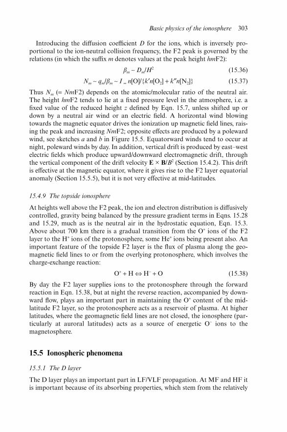
Introducing the diffusion coefficient D for the ions, which is inversely pro-portional to the ion-neutral collision frequency, the F2 peak is governed by therelations (in which the suffix m denotes values at the peak height hmF2):
βm ∼ Dm/H2 (15.36)
Nm ∼ qm/βm ∼ I ∞ n[O]/{k′n[O2] + k″n[N2]} (15.37)
Thus Nm (= NmF2) depends on the atomic/molecular ratio of the neutral air.The height hmF2 tends to lie at a fixed pressure level in the atmosphere, i.e. afixed value of the reduced height z defined by Eqn. 15.7, unless shifted up ordown by a neutral air wind or an electric field. A horizontal wind blowingtowards the magnetic equator drives the ionization up magnetic field lines, rais-ing the peak and increasing NmF2; opposite effects are produced by a polewardwind, see sketches a and b in Figure 15.5. Equatorward winds tend to occur atnight, poleward winds by day. In addition, vertical drift is produced by east–westelectric fields which produce upward/downward electromagnetic drift, throughthe vertical component of the drift velocity E × B/B2 (Section 15.4.2). This driftis effective at the magnetic equator, where it gives rise to the F2 layer equatorialanomaly (Section 15.5.5), but it is not very effective at mid-latitudes.
15.4.9 The topside ionosphere
At heights well above the F2 peak, the ion and electron distribution is diffusivelycontrolled, gravity being balanced by the pressure gradient terms in Eqns. 15.28and 15.29, much as is the neutral air in the hydrostatic equation, Eqn. 15.3.Above about 700 km there is a gradual transition from the O+ ions of the F2layer to the H+ ions of the protonosphere, some He+ ions being present also. Animportant feature of the topside F2 layer is the flux of plasma along the geo-magnetic field lines to or from the overlying protonosphere, which involves thecharge-exchange reaction:
O+ + H ⇔ H− + O (15.38)
By day the F2 layer supplies ions to the protonosphere through the forwardreaction in Eqn. 15.38, but at night the reverse reaction, accompanied by down-ward flow, plays an important part in maintaining the O+ content of the mid-latitude F2 layer, so the protonosphere acts as a reservoir of plasma. At higherlatitudes, where the geomagnetic field lines are not closed, the ionosphere (par-ticularly at auroral latitudes) acts as a source of energetic O− ions to themagnetosphere.
15.5 Ionospheric phenomena
15.5.1 The D layer
The D layer plays an important part in LF/VLF propagation. At MF and HF itis important because of its absorbing properties, which stem from the relatively
Basic physics of the ionosphere 303
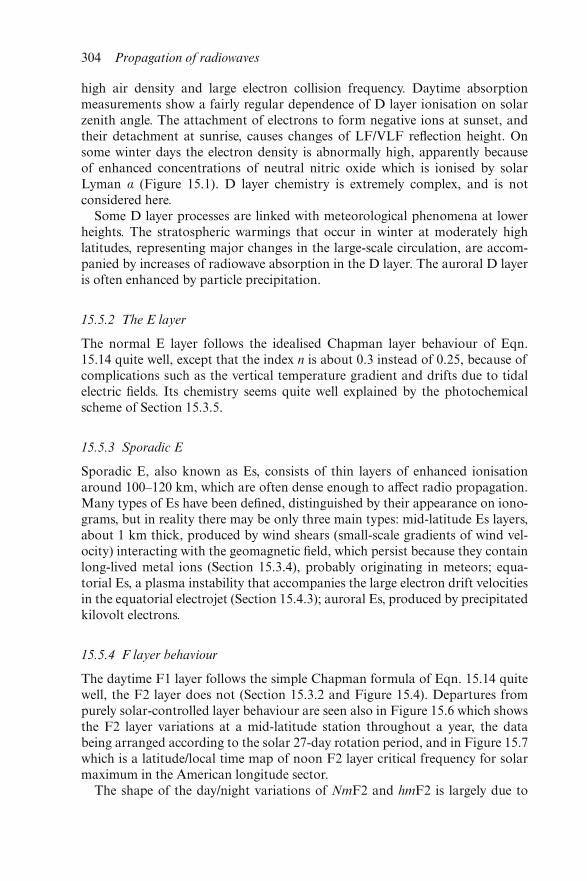
high air density and large electron collision frequency. Daytime absorptionmeasurements show a fairly regular dependence of D layer ionisation on solarzenith angle. The attachment of electrons to form negative ions at sunset, andtheir detachment at sunrise, causes changes of LF/VLF reflection height. Onsome winter days the electron density is abnormally high, apparently becauseof enhanced concentrations of neutral nitric oxide which is ionised by solarLyman α (Figure 15.1). D layer chemistry is extremely complex, and is notconsidered here.
Some D layer processes are linked with meteorological phenomena at lowerheights. The stratospheric warmings that occur in winter at moderately highlatitudes, representing major changes in the large-scale circulation, are accom-panied by increases of radiowave absorption in the D layer. The auroral D layeris often enhanced by particle precipitation.
15.5.2 The E layer
The normal E layer follows the idealised Chapman layer behaviour of Eqn.15.14 quite well, except that the index n is about 0.3 instead of 0.25, because ofcomplications such as the vertical temperature gradient and drifts due to tidalelectric fields. Its chemistry seems quite well explained by the photochemicalscheme of Section 15.3.5.
15.5.3 Sporadic E
Sporadic E, also known as Es, consists of thin layers of enhanced ionisationaround 100–120 km, which are often dense enough to affect radio propagation.Many types of Es have been defined, distinguished by their appearance on iono-grams, but in reality there may be only three main types: mid-latitude Es layers,about 1 km thick, produced by wind shears (small-scale gradients of wind vel-ocity) interacting with the geomagnetic field, which persist because they containlong-lived metal ions (Section 15.3.4), probably originating in meteors; equa-torial Es, a plasma instability that accompanies the large electron drift velocitiesin the equatorial electrojet (Section 15.4.3); auroral Es, produced by precipitatedkilovolt electrons.
15.5.4 F layer behaviour
The daytime F1 layer follows the simple Chapman formula of Eqn. 15.14 quitewell, the F2 layer does not (Section 15.3.2 and Figure 15.4). Departures frompurely solar-controlled layer behaviour are seen also in Figure 15.6 which showsthe F2 layer variations at a mid-latitude station throughout a year, the databeing arranged according to the solar 27-day rotation period, and in Figure 15.7which is a latitude/local time map of noon F2 layer critical frequency for solarmaximum in the American longitude sector.
The shape of the day/night variations of NmF2 and hmF2 is largely due to
304 Propagation of radiowaves
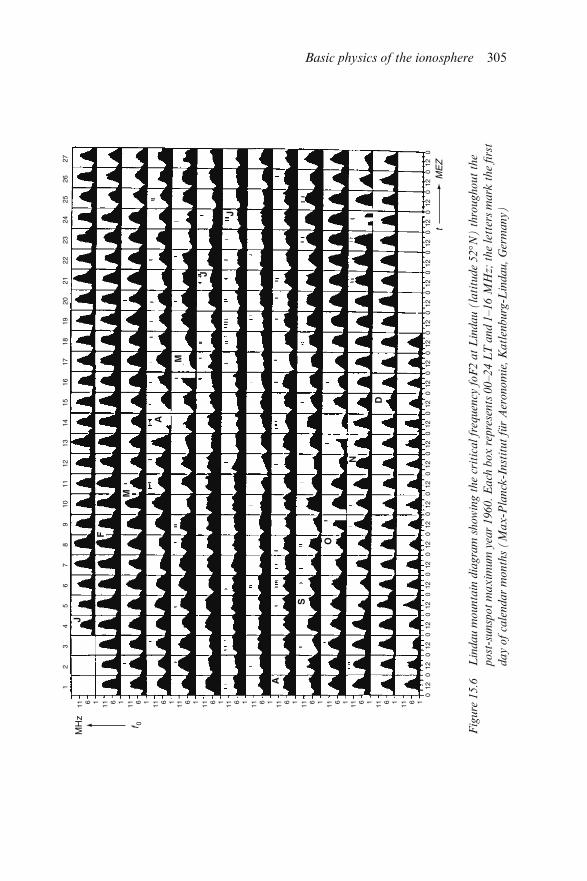
Fig
ure
15.6
Lin
dau m
ounta
in d
iagra
m s
how
ing t
he
crit
ical
freq
uen
cy f
oF
2 a
t L
indau (
lati
tude
52°N
) t
hro
ughout
the
post
-sunsp
ot
max
imum
yea
r 1960.
Each
box
rep
rese
nts
00–24 L
T a
nd 1
–16 M
Hz;
the
lett
ers
mark
the
firs
t
day o
f ca
lendar
month
s (M
ax
-Pla
nck
-Inst
itut
für
Aer
onom
ie,
Katl
enburg
-Lin
dau,
Ger
many)
Basic physics of the ionosphere 305
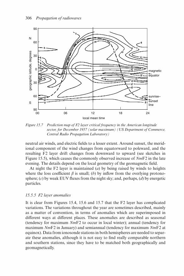
neutral air winds, and electric fields to a lesser extent. Around sunset, the merid-ional component of the wind changes from equatorward to poleward, and theresulting F2 layer drift changes from downward to upward (see sketches inFigure 15.5), which causes the commonly observed increase of NmF2 in the lateevening. The details depend on the local geometry of the geomagnetic field.
At night the F2 layer is maintained (a) by being raised by winds to heightswhere the loss coefficient β is small; (b) by inflow from the overlying protono-sphere; (c) by weak EUV fluxes from the night sky; and, perhaps, (d) by energeticparticles.
15.5.5 F2 layer anomalies
It is clear from Figures 15.4, 15.6 and 15.7 that the F2 layer has complicatedvariations. The variations throughout the year are sometimes described, mainlyas a matter of convention, in terms of anomalies which are superimposed indifferent ways at different places. These anomalies are described as seasonal(tendency for maximum NmF2 to occur in local winter); annual (tendency formaximum NmF2 in January) and semiannual (tendency for maximum NmF2 atequinox). Data from ionosonde stations in both hemispheres are needed to separ-ate these anomalies, although it is not easy to find really comparable northernand southern stations, since they have to be matched both geographically andgeomagnetically.
Figure 15.7 Prediction map of F2 layer critical frequency in the American longitude
sector, for December 1957 (solar maximum) (US Department of Commerce,
Central Radio Propagation Laboratory)
306 Propagation of radiowaves
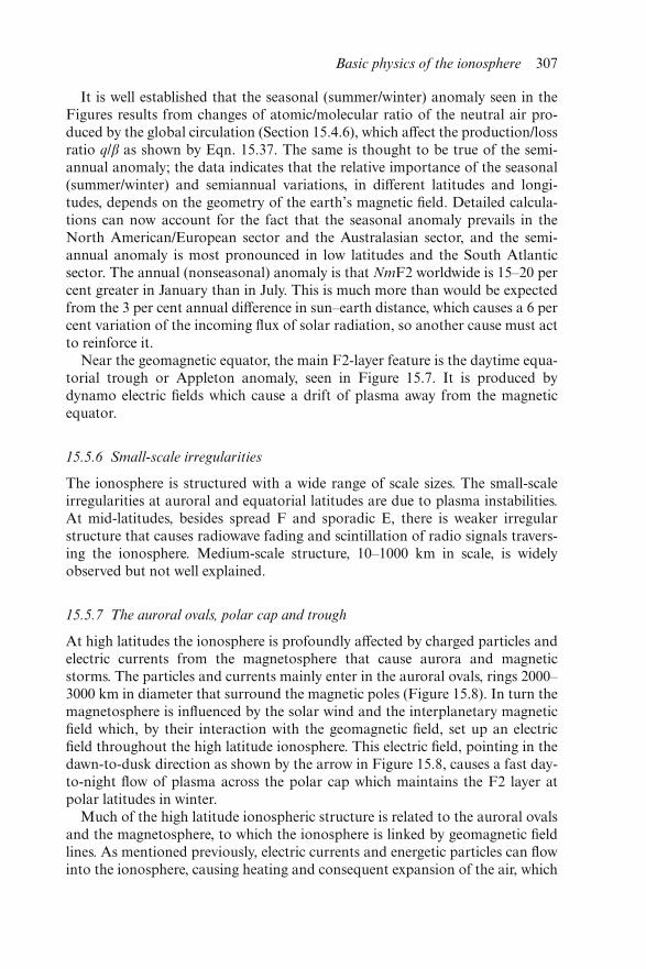
It is well established that the seasonal (summer/winter) anomaly seen in theFigures results from changes of atomic/molecular ratio of the neutral air pro-duced by the global circulation (Section 15.4.6), which affect the production/lossratio q/β as shown by Eqn. 15.37. The same is thought to be true of the semi-annual anomaly; the data indicates that the relative importance of the seasonal(summer/winter) and semiannual variations, in different latitudes and longi-tudes, depends on the geometry of the earth’s magnetic field. Detailed calcula-tions can now account for the fact that the seasonal anomaly prevails in theNorth American/European sector and the Australasian sector, and the semi-annual anomaly is most pronounced in low latitudes and the South Atlanticsector. The annual (nonseasonal) anomaly is that NmF2 worldwide is 15–20 percent greater in January than in July. This is much more than would be expectedfrom the 3 per cent annual difference in sun–earth distance, which causes a 6 percent variation of the incoming flux of solar radiation, so another cause must actto reinforce it.
Near the geomagnetic equator, the main F2-layer feature is the daytime equa-torial trough or Appleton anomaly, seen in Figure 15.7. It is produced bydynamo electric fields which cause a drift of plasma away from the magneticequator.
15.5.6 Small-scale irregularities
The ionosphere is structured with a wide range of scale sizes. The small-scaleirregularities at auroral and equatorial latitudes are due to plasma instabilities.At mid-latitudes, besides spread F and sporadic E, there is weaker irregularstructure that causes radiowave fading and scintillation of radio signals travers-ing the ionosphere. Medium-scale structure, 10–1000 km in scale, is widelyobserved but not well explained.
15.5.7 The auroral ovals, polar cap and trough
At high latitudes the ionosphere is profoundly affected by charged particles andelectric currents from the magnetosphere that cause aurora and magneticstorms. The particles and currents mainly enter in the auroral ovals, rings 2000–3000 km in diameter that surround the magnetic poles (Figure 15.8). In turn themagnetosphere is influenced by the solar wind and the interplanetary magneticfield which, by their interaction with the geomagnetic field, set up an electricfield throughout the high latitude ionosphere. This electric field, pointing in thedawn-to-dusk direction as shown by the arrow in Figure 15.8, causes a fast day-to-night flow of plasma across the polar cap which maintains the F2 layer atpolar latitudes in winter.
Much of the high latitude ionospheric structure is related to the auroral ovalsand the magnetosphere, to which the ionosphere is linked by geomagnetic fieldlines. As mentioned previously, electric currents and energetic particles can flowinto the ionosphere, causing heating and consequent expansion of the air, which
Basic physics of the ionosphere 307
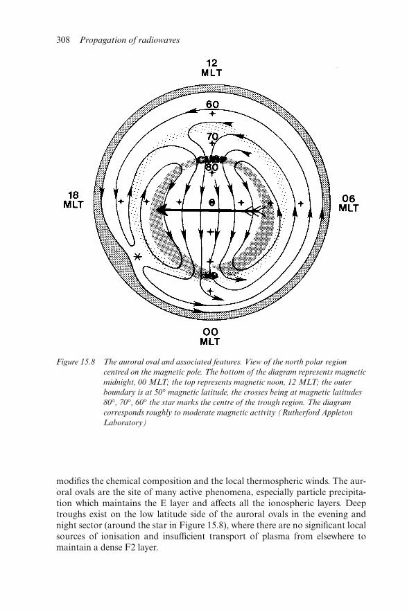
modifies the chemical composition and the local thermospheric winds. The aur-oral ovals are the site of many active phenomena, especially particle precipita-tion which maintains the E layer and affects all the ionospheric layers. Deeptroughs exist on the low latitude side of the auroral ovals in the evening andnight sector (around the star in Figure 15.8), where there are no significant localsources of ionisation and insufficient transport of plasma from elsewhere tomaintain a dense F2 layer.
Figure 15.8 The auroral oval and associated features. View of the north polar region
centred on the magnetic pole. The bottom of the diagram represents magnetic
midnight, 00 MLT; the top represents magnetic noon, 12 MLT; the outer
boundary is at 50° magnetic latitude, the crosses being at magnetic latitudes
80°, 70°, 60° the star marks the centre of the trough region. The diagram
corresponds roughly to moderate magnetic activity (Rutherford Appleton
Laboratory)
308 Propagation of radiowaves
15.6 Solar–terrestrial relations and ionospheric storms
15.6.1 Solar flares and sudden ionospheric disturbances
The intense X-rays from solar flares produce strong enhancements of electrondensity in the D layer, giving rise to sudden ionospheric disturbances (SID), aterm which embraces radio shortwave fadeouts, effects on LF/VLF propagationand magnetic perturbations. These occur in the sunlit hemisphere and typicallylast for half an hour. Soon afterwards MeV particles from the flare arrive andcause enhanced radio absorption at high latitudes (polar cap absorption, PCA).
15.6.2 Geomagnetic storms
Streams of plasma ejected from the solar corona travel outwards as gusts in thesolar wind, taking about 24 hours to reach the earth. The impact of a plasmastream on the magnetosphere causes a magnetic storm, starting with a compres-sion of the geomagnetic field observed at the ground as a storm sudden com-mencement (SSC). The interaction of the plasma stream and the magnetospheresets up a ring current around the earth, mainly carried by keV ions, which causesa decrease of the geomagnetic field, greatest at 12–24 hours after the SSC anddecaying in 2–3 days. The auroral oval expands equatorwards and associatedionospheric features move to lower latitudes during the storm.
15.6.3 Ionospheric storms
During a geomagnetic storm, particle precipitation at high latitudes producesdisturbances at D layer heights, probably chemical in nature, such as through theproduction of extra nitric oxide which is then ionised by solar Lyman α. Theeffects are propagated to the mid-latitude D layer, where they last for severaldays. The F2 layer is often profoundly affected during magnetic storms, withsevere effects on radio propagation. At mid-latitudes the F2 layer electron dens-ity initially increases, then decreases during the main phase, and recovers in2–3 days. Examples of these negative storm effects can be seen in Figure 15.6.In winter, however, there is often a positive effect, i.e. an increase of F2 layerdensity in the main phase. Storm effects are very complicated, with many differ-ences between individual events that depend on place, the time of year and thelocal time when the storm begins, so summarised descriptions can bemisleading.
The F2 layer storm effects are largely due to changes of temperature and thehorizontal and vertical thermospheric winds, driven by the enhanced heating inthe auroral zone which modifies the quiet day wind system shown in Figure 15.2.Equatorward winds are enhanced, causing lifting of the F2 layer which affectsNmF2 in the manner shown in Figure 15.5. The equatorward winds bring airwith an enhanced molecular/atomic ratio from high latitudes to mid-latitudes,which in turn increases the loss coefficient β (see Eqn. 15.37) and hence decreases
Basic physics of the ionosphere 309
NmF2 at mid-latitudes; this is the main cause of negative storm effects at mid-latitudes. Positive F2 layer storm effects in winter and at low latitudes are due todecreases of molecular/atomic ratio, induced by increased downward airmotions, or to lifting produced by winds or by enhanced electric fields.
15.6.4 Space weather
The ionosphere is part of the space environment, and space weather includes theshort-term variability of the ionosphere, which is still not well understood. Itsmajor aspects are the vagaries of sporadic E and of the F2 layer. At mid-latitudes, day-to-day variability of NmF2 is typically 20 per cent by day and30 per cent at night: the factors thought to cause it are geomagnetic distur-bance, waves and tides transmitted from the lower atmosphere and variationsof the incoming solar photon radiation, which is probably a minor factor as faras day-to-day variations are concerned.
15.6.5 Long-term change
This is a different kind of disturbance! Increasing concentrations of carbondioxide and methane that cause global warming in the lower atmosphere resultin global cooling in the upper atmosphere (because of the enhanced loss of heatto space by infrared radiation). If the mesospheric concentrations of these gasesare doubled in, say, the next fifty years, as is anticipated, it is estimated that:
• the mean tropospheric temperature will increase by 1–2 K
• the mean mesospheric temperature will decrease by 5 K
• the mean exospheric temperature will decrease by 40 K
The resulting thermal contraction of the thermosphere will decrease the airdensity at 300 km by about 40 per cent, thereby prolonging satellite lifetimes,and lower the E layer by about 2 km and F2 layer by 20 km, with some change ofMUF. There is experimental evidence that mesospheric temperature hasdecreased in recent decades, and lowering of hmF2 has been reported at somestations, although the observations do not give a clear-cut result, as there appearto be regional variations. Other possible long-term effects are changes in upperatmosphere tides, resulting from the depletion of the ozone layer where sometidal forcing originates, and chemical contamination by spacecraft launches.
15.7 Conclusions
Contemporary ionospheric science has many aspects: as a branch of solar-terrestrial physics and the earth’s environment; the science of radiocommunica-tions, e.g. predicting and forecasting; the mathematics of wave propagation inthe ionosphere; man-made radio transmissions, and natural electromagneticemissions, magnetic pulsations and other phenomena. As a natural plasma,
310 Propagation of radiowaves
often nonlinear and nonthermal, the ionosphere is a site for active experimentswith radiowaves, powerful enough to produce observable ionospheric modifi-cations, in the form of increased temperatures and plasma instabilities, and withchemical releases and particle beam experiments. Such ionospheric plasmaphysics experiments provide new physical insights, although they often raisemore questions than they solve.
Problems remain at the upper and lower boundaries; i.e. the interactions withthe lower atmosphere and the magnetosphere, and how their effects spreadworldwide. Large electric fields generated in thunderstorms can affect theionosphere. There are suggestions of topographic influences, e.g. of mountainranges, on the ionosphere. The reverse question of ionospheric, geomagneticand solar effects on weather and climate is contentious; possible relationsbetween magnetic and solar disturbance and the weather have been found, buttheir physical mechanisms are not well established.
The basic mechanisms of the ionosphere seem to be known, but surprises arepossible in any active area of science, and many questions remain. The everydaymonitoring of this important part of the environment is as vital for progress inthe future as it has been in the past.
15.8 Bibliography
JURSA, A.S. (Ed.): ‘Handbook of geophysics and the space environment’ (AirForce Geophysics Laboratory, Bedford, Mass., 1985)HARGREAVES, J.K.: ‘The upper atmosphere and solar-terrestrial environment’(Cambridge University Press, 1992)RATCLIFFE, J.A.: ‘Sun, earth and radio’ (World University Library, 1970)RISHBETH, H., and GARRIOTT, O.K: ‘Introduction to ionospheric physics’(Academic, New York, 1969)RUSSELL, C.T. and KIVELSON, M.: ‘Introduction to space physics’(Cambridge University Press, 1995)SCHUNK, R.W., and NAGY, A.F.: ‘Ionospheres: physics, plasma physics andchemistry’ (Cambridge University Press, 2000)TASCIONE, T.F.: ‘Introduction to the space environment’ (Orbit, 1988)
Basic physics of the ionosphere 311

Chapter 16
Ionospheric propagation
Paul S. Cannon and Peter A. Bradley
16.1 A systems perspective
The ionosphere, which extends from ∼60 km to ∼1000 km, significantly affectsthe propagation of high-frequency (HF) to ultrahigh-frequency (UHF) signalswhich pass through it. The effects are varied but include refraction, retardationand scintillation. Ground–ground HF communications systems, ground–spacecommunications systems, single frequency GPS (global positioning system),HF over-the-horizon radars, satellite altimeters and space-based radars [1] areexamples of radio systems constrained by this medium.
HF communications and radar systems are of course dependent on theionosphere for long distance operation but most systems are degraded by theionosphere. Loss of phase lock and range errors in GPS are examples of suchdeleterious effects.
As with all radio systems the design of ionospheric systems must address theissues of signal-to-noise plus interference ratio (SNR), multipath and Dopplershift and spread. For many systems, however, signal group delay, phase scintilla-tion and other issues are also important. Table 16.1 provides quantitative esti-mates of some of these effects.
For ionospheric signals the SNR is determined by a number of factors. ForHF signals whether the signal is actually reflected by the ionosphere is critical.All transionospheric signals also experience some excess attenuation over freespace but, as we will see, because this is frequency dependent, the effects athigher frequencies are generally negligible. In the HF band interferencedominates over the noise but further discussion falls outside of the remit of thisChapter. The reader is referred to Reference [2] for further discussion.
Multipath arises from various sources. A transmitted HF signal can bereflected from more than one of the several layers in the ionosphere. The trans-mission of a single pulse of energy is consequently received as a number of
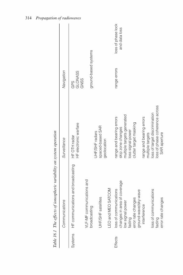
Tabl
e 16.1
The
effec
ts o
f io
nosp
her
ic v
ari
abil
ity o
n s
yst
em o
per
ati
on
Com
mun
icat
ions
Sur
veill
ance
Nav
igat
ion
Sys
tem
sH
F co
mm
unic
atio
ns a
nd b
road
cast
ing
HF
OTH
rad
arH
F el
ectro
nic
war
fare
GP
SG
LON
AS
SG
NS
SV
LF-M
F co
mm
unic
atio
ns a
ndb
road
cast
ing
gro
und
-bas
ed s
yste
ms
UH
F/S
HF
sate
llite
s
LEO
and
ME
O S
ATC
OM
UH
F/S
HF
rad
ars
spac
ed-b
ased
SA
Rg
eolo
catio
n
Effe
cts
loss
of c
omm
unic
atio
nsch
ang
es in
are
a of
cov
erag
elo
w s
igna
l pow
erfa
din
ger
ror r
ate
chan
ges
gro
und
-wav
e/sk
y-w
ave
inte
rfer
ence
loss
of c
omm
unic
atio
nsfa
din
ger
ror r
ate
chan
ges
rang
e an
d b
earin
g e
rror
ssk
ip z
one
chan
ges
mul
tiple
targ
ets
gen
erat
edlo
ss s
igna
l pow
ercl
utte
r tar
get
mas
king
rang
e an
d b
earin
g e
rror
sm
ultip
le ta
rget
slo
ss o
f tar
get
dis
crim
inat
ion
loss
of p
hase
coh
eren
ce a
cros
sS
AR
ap
ertu
re
rang
e er
rors
loss
of p
hase
lock
and
dat
a lo
ss
314 Propagation of radiowaves
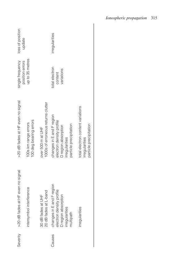
Sev
erity
>20
dB
fad
es a
t HF
even
no
sig
nal
inte
rsym
bol
inte
rfer
ence
30 d
B fa
des
at U
HF
20 d
B fa
des
at L
-ban
d
>20
dB
fad
es a
t HF
even
no
sig
nal
100s
km
rang
e er
rors
100
deg
bea
ring
err
ors
over
500
m a
t UH
F10
00s
of e
rron
eous
retu
rns
clut
ter
sing
le fr
eque
ncy
pos
ition
err
ors
up to
35
met
res
loss
of p
ositi
onup
dat
e
Cau
ses
chan
ges
in E
and
F re
gio
nel
ectro
n d
ensi
ty p
rofil
eD
reg
ion
abso
rptio
nirr
egul
ariti
esm
ultip
ath
irreg
ular
ities
chan
ges
in E
and
F re
gio
nel
ectro
n d
ensi
ty p
rofil
eD
reg
ion
abso
rptio
nirr
egul
ariti
esp
artic
le p
reci
pita
tion
tota
l ele
ctro
n co
nten
t var
iatio
nsirr
egul
ariti
esp
artic
le p
reci
pita
tion
tota
l ele
ctro
nco
nten
tva
riatio
ns
irreg
ular
ities
Ionospheric propagation 315
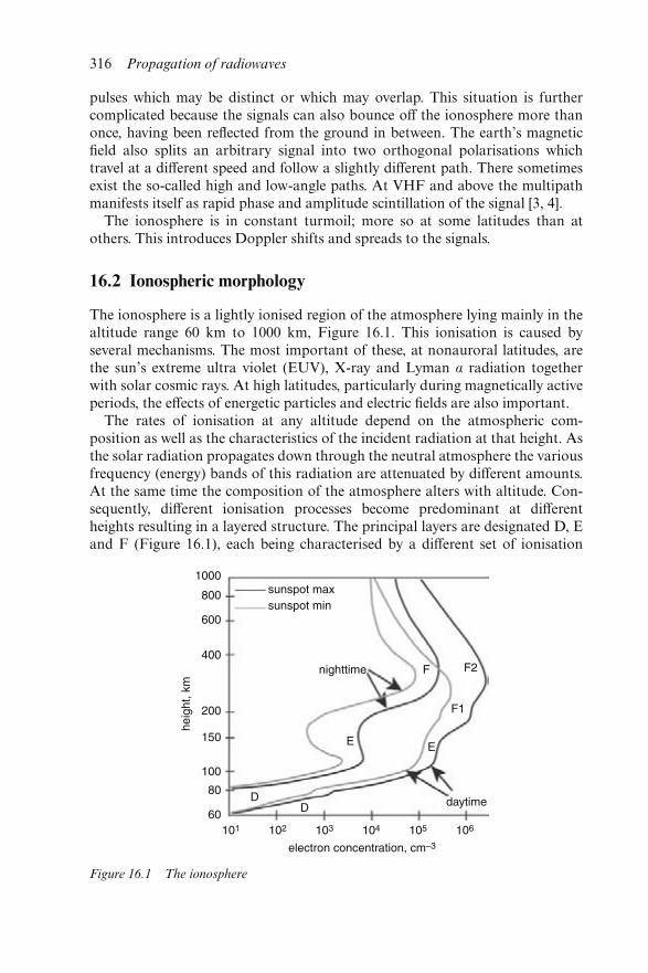
pulses which may be distinct or which may overlap. This situation is furthercomplicated because the signals can also bounce off the ionosphere more thanonce, having been reflected from the ground in between. The earth’s magneticfield also splits an arbitrary signal into two orthogonal polarisations whichtravel at a different speed and follow a slightly different path. There sometimesexist the so-called high and low-angle paths. At VHF and above the multipathmanifests itself as rapid phase and amplitude scintillation of the signal [3, 4].
The ionosphere is in constant turmoil; more so at some latitudes than atothers. This introduces Doppler shifts and spreads to the signals.
16.2 Ionospheric morphology
The ionosphere is a lightly ionised region of the atmosphere lying mainly in thealtitude range 60 km to 1000 km, Figure 16.1. This ionisation is caused byseveral mechanisms. The most important of these, at nonauroral latitudes, arethe sun’s extreme ultra violet (EUV), X-ray and Lyman α radiation togetherwith solar cosmic rays. At high latitudes, particularly during magnetically activeperiods, the effects of energetic particles and electric fields are also important.
The rates of ionisation at any altitude depend on the atmospheric com-position as well as the characteristics of the incident radiation at that height. Asthe solar radiation propagates down through the neutral atmosphere the variousfrequency (energy) bands of this radiation are attenuated by different amounts.At the same time the composition of the atmosphere alters with altitude. Con-sequently, different ionisation processes become predominant at differentheights resulting in a layered structure. The principal layers are designated D, Eand F (Figure 16.1), each being characterised by a different set of ionisation
Figure 16.1 The ionosphere
316 Propagation of radiowaves
processes. These regions are themselves layered or structured into the E, Es, F1and F2 regions. The number of layers, their heights and their ionisation densityvary with time and in space. The high latitude ionosphere is particularly compli-cated and will not be dealt with here, but is described in Reference [5].
16.3 Theory of propagation in the ionosphere
16.3.1 Vertical propagation – no collisions
The ionosphere is a dispersive medium, that is to say the refractive index of themedium varies as a function of frequency. As a consequence, different frequen-cies travel with different speeds causing spreading of the pulse. The ionosphere isalso layered, as we have described, and this leads to multipath propagation. Theearth’s magnetic field introduces a further complication in as much as it rendersthe ionosphere anisotropic. This means that the incident ray will be split intotwo rays on entering the ionosphere in a manner similar to that of crystal optics.The two differently polarised rays are referred to as ordinary (O) and extra-ordinary (X). One result of this splitting is the phenomenon of Faraday rotationof the plane of polarisation as it traverses the ionosphere. The ionosphere,however, is above all a region where the refractive index is less than unity result-ing in a group velocity which is less than that of light in free space. A con-sequence of this is that vertically launched rays can be reflected and oblique raysare progressively bent away from the vertical. Obliquely launched HF rays can infact be turned back towards the ground providing the phenomenon of sky-wavecommunications.
A fundamental ionospheric propagation equation is the Appleton-Lassenformula, which describes the complex refractive index, n2. In particular, theequation describes the propagation of HF waves. When collisions betweenthe electrons and neutrals are negligible (in the E and F regions) the real part ofthe refractive index μ can be determined from a simplified form of the Appleton-Lassen formula:
μ2 = 1 −2X(1 − X)
2(1 − X) − Y 2T ± [Y 4
T + 4(1 − X)2Y 2L]1/2
(16.1)
where
X = Ne2
ε0mω2, YL =
eBL
mω and YT =
eBT
mω(16.2)
The subscripts T and L refer to transverse and longitudinal components of theimposed geomagnetic flux (B) with reference to the direction of the wave normalof propagation. N is the electron density, e is the charge on the electron, m is themass of the electron, ε0 is the permittivity of free space and ω is the angular wavefrequency. The plus sign above refers to the ordinary wave and the minus signrefers to the extraordinary wave.
If, the magnetic field is ignored the above reduces to:
Ionospheric propagation 317
μ2 = 1 − X = 1 − �fN
f �2
= 1 − kN
f 2(16.3)
where
fN = �Ne2
ε0m�
0.5
(16.4)
This parameter, fN, is known as the plasma or critical frequency. The constant
k = 80.5 (16.5)
when N is in electrons per cubic metre and f is in Hz.Reflection at vertical incidence occurs when μ = 0, i.e. when f = fN. At higher
frequencies, where f > fN, the refractive index never drops to zero, reflectionnever occurs and the vertical ray passes through the ionosphere into space. Thisis the normal condition for signals above the HF band.
16.3.2 Group path and phase path
Two important concepts in ionospheric radio propagation are those of grouppath and phase path. Due to the embedded geomagnetic field the ionosphere isanisotropic, that is the phase velocity, ν, of the wave is dependent on direction.As a consequence the phase paths and group paths differ. It can be shown thatthe angle α between the wave normal and the ray direction is given by:
tan α = −1
ν
dν
dθ = +
1
μ
dμ
dθ(16.6)
where θ is the angle at which the wave normal direction cuts a reference axis. Thephase path in an anisotropic medium is:
P = �s
μ cos α ds (16.7)
integrated over the ray path s. The corresponding group path, P′ is:
P′ = �s
μ′ cos α ds (16.8)
where μ′ is the group refractive index such that:
μ′ = c
μ(16.9)
16.3.3 Oblique propagation
Obliquely launched HF rays can also return to the ground, and this can even
318 Propagation of radiowaves
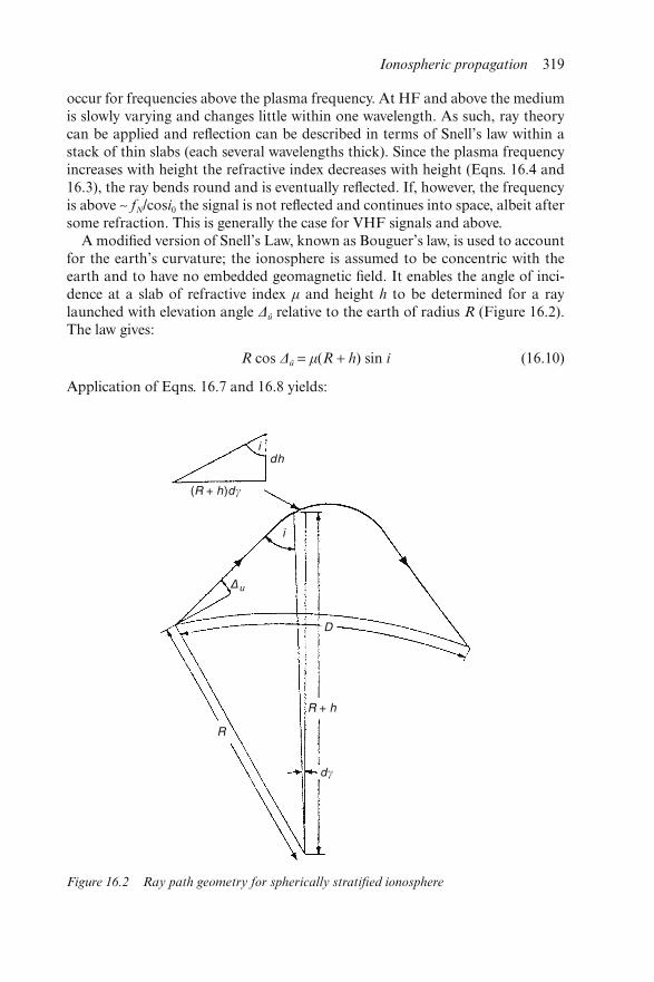
occur for frequencies above the plasma frequency. At HF and above the mediumis slowly varying and changes little within one wavelength. As such, ray theorycan be applied and reflection can be described in terms of Snell’s law within astack of thin slabs (each several wavelengths thick). Since the plasma frequencyincreases with height the refractive index decreases with height (Eqns. 16.4 and16.3), the ray bends round and is eventually reflected. If, however, the frequencyis above ∼ fN/cosi0 the signal is not reflected and continues into space, albeit aftersome refraction. This is generally the case for VHF signals and above.
A modified version of Snell’s Law, known as Bouguer’s law, is used to accountfor the earth’s curvature; the ionosphere is assumed to be concentric with theearth and to have no embedded geomagnetic field. It enables the angle of inci-dence at a slab of refractive index μ and height h to be determined for a raylaunched with elevation angle Δû relative to the earth of radius R (Figure 16.2).The law gives:
R cos Δû = μ(R + h) sin i (16.10)
Application of Eqns. 16.7 and 16.8 yields:
Figure 16.2 Ray path geometry for spherically stratified ionosphere
Ionospheric propagation 319
P = �h
0
μ dh
cos i = �
h
0
μ2 dh
�μ2 − � R
R + h�2
cos2 Δu
(16.11)
P = �h
0
dh
�μ2 − � R
R + h�2
cos2 Δu
(16.12)
and
D = R�γ
0
dγ = R �h
0
tan i dh
R + h = R2 cos Δu�
h
0
dh
(R + h)2�μ2 − � R
R + h�2
cos2 Δu
(16.13)
In reality of course the ray paths travel in an ionosphere which is not concentricand which has a magnetic field. Often, we find, however, that approximationssuch as the one just described provide adequate accuracy. This is particularlytrue at mid-latitudes.
16.3.4 Absorption
If the effects of collisions are included then Eqn. 16.1 becomes more compli-cated via the introduction of a term Z = ν/ω, where ν is the electron-neutralcollision frequency:
n2 = (μ − iχ)2 = 1 − X
1 − iZ −Y 2
T
2(1 − X − iZ)± � Y 4
T
4(1 − X − iZ)2+ Y 2
z
(16.14)
For a wave travelling in the z direction at time, t:
E = E0 exp i�ωt − w
cnz� (16.15)
where, c is the velocity of light, or:
E = E0 exp�− ω
cχz� exp i�ωt −
w
cμz� 16.16)
If χ, the imaginary term in the refractive index, is nonzero the quantity (ωχ/c)is a measure of the decay of amplitude per unit distance and is called theabsorption coefficient, κ (kappa):
κ = ωχ
c(16.17)
320 Propagation of radiowaves
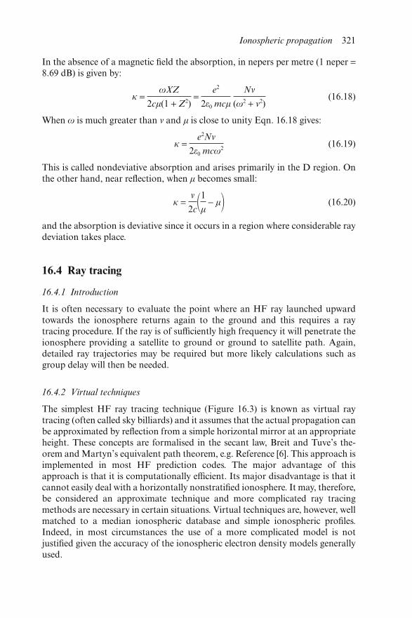
In the absence of a magnetic field the absorption, in nepers per metre (1 neper =8.69 dB) is given by:
κ = ωXZ
2cμ(1 + Z2) =
e2
2ε0 mcμ
Nν
(ω2 + ν2)(16.18)
When ω is much greater than ν and μ is close to unity Eqn. 16.18 gives:
κ = e2Nν
2ε0 mcω2(16.19)
This is called nondeviative absorption and arises primarily in the D region. Onthe other hand, near reflection, when μ becomes small:
κ = v
2c�1
μ − μ� (16.20)
and the absorption is deviative since it occurs in a region where considerable raydeviation takes place.
16.4 Ray tracing
16.4.1 Introduction
It is often necessary to evaluate the point where an HF ray launched upwardtowards the ionosphere returns again to the ground and this requires a raytracing procedure. If the ray is of sufficiently high frequency it will penetrate theionosphere providing a satellite to ground or ground to satellite path. Again,detailed ray trajectories may be required but more likely calculations such asgroup delay will then be needed.
16.4.2 Virtual techniques
The simplest HF ray tracing technique (Figure 16.3) is known as virtual raytracing (often called sky billiards) and it assumes that the actual propagation canbe approximated by reflection from a simple horizontal mirror at an appropriateheight. These concepts are formalised in the secant law, Breit and Tuve’s the-orem and Martyn’s equivalent path theorem, e.g. Reference [6]. This approach isimplemented in most HF prediction codes. The major advantage of thisapproach is that it is computationally efficient. Its major disadvantage is that itcannot easily deal with a horizontally nonstratified ionosphere. It may, therefore,be considered an approximate technique and more complicated ray tracingmethods are necessary in certain situations. Virtual techniques are, however, wellmatched to a median ionospheric database and simple ionospheric profiles.Indeed, in most circumstances the use of a more complicated model is notjustified given the accuracy of the ionospheric electron density models generallyused.
Ionospheric propagation 321
16.4.2.1 Simple transionospheric models
A radio signal, which penetrates the anisotropic ionosphere, is modified in anumber of ways. Both large-scale changes due to variations in the electrondensity and small-scale irregularities affect the signal. The effects include scintil-lation, absorption, variations in the direction of arrival, group path delay, dis-persion, Doppler shift, polarisation rotation, refraction and phase advances. Allof these effects are proportional to the total electron content, NT, or its timederivative and inversely proportional to frequency to the appropriate power.(The total electron content (TEC) is the total number of electrons in a columnof unit area, along the path from the transmitter to the receiver.) For frequencieswell above the critical frequency the following simple relationships can be used:
RF carrier phase advance:
ΔΦ = 8.44 × 10⁻¹³
fNT (radians) (16.21)
where NT is measured in electrons.m−2 and the frequency f is measured in Hz.
Group path delay: the excess time delay, over the free space transit time is givenby:
Δt = 40.3
cf 2NT (s) (16.22)
Distortion of pulse waveforms: the ionospheric dispersion causes pulse broaden-ing by virtue of the differential time delay across the signal bandwidth, Δf
according to:
Δt = 80.6 × 10⁶
cf 3ΔfNT(s) (16.23)
Faraday rotation: At frequencies above 100 MHz this may be approximated by:
Figure 16.3 Geometry for ray propagation; earth and ionosphere are plane surfaces; the
transmitter and receiver are at T (t) and R (r) respectively, the true point of
reflection is at B (b) and the virtual point of reflection is at A (a)
322 Propagation of radiowaves
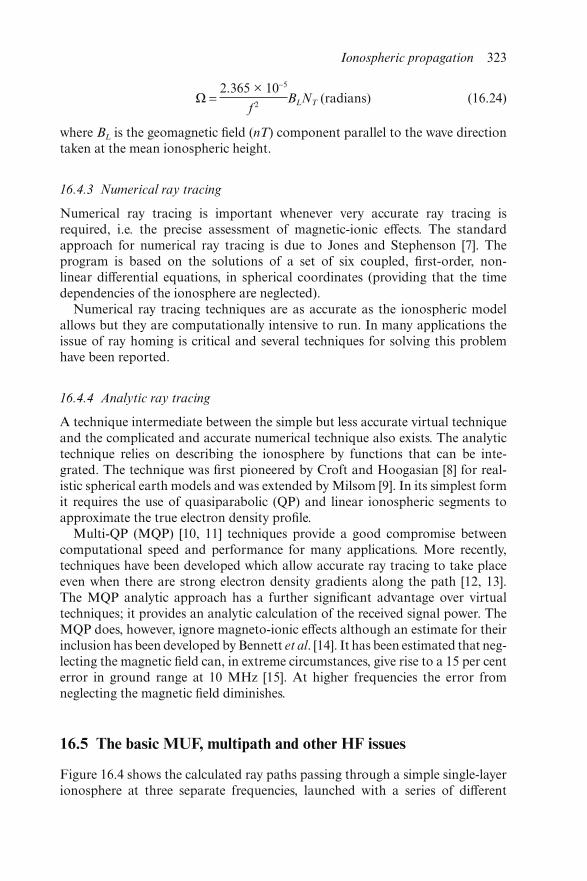
Ω = 2.365 × 10⁻⁵
f 2BLNT (radians) (16.24)
where BL is the geomagnetic field (nT) component parallel to the wave directiontaken at the mean ionospheric height.
16.4.3 Numerical ray tracing
Numerical ray tracing is important whenever very accurate ray tracing isrequired, i.e. the precise assessment of magnetic-ionic effects. The standardapproach for numerical ray tracing is due to Jones and Stephenson [7]. Theprogram is based on the solutions of a set of six coupled, first-order, non-linear differential equations, in spherical coordinates (providing that the timedependencies of the ionosphere are neglected).
Numerical ray tracing techniques are as accurate as the ionospheric modelallows but they are computationally intensive to run. In many applications theissue of ray homing is critical and several techniques for solving this problemhave been reported.
16.4.4 Analytic ray tracing
A technique intermediate between the simple but less accurate virtual techniqueand the complicated and accurate numerical technique also exists. The analytictechnique relies on describing the ionosphere by functions that can be inte-grated. The technique was first pioneered by Croft and Hoogasian [8] for real-istic spherical earth models and was extended by Milsom [9]. In its simplest formit requires the use of quasiparabolic (QP) and linear ionospheric segments toapproximate the true electron density profile.
Multi-QP (MQP) [10, 11] techniques provide a good compromise betweencomputational speed and performance for many applications. More recently,techniques have been developed which allow accurate ray tracing to take placeeven when there are strong electron density gradients along the path [12, 13].The MQP analytic approach has a further significant advantage over virtualtechniques; it provides an analytic calculation of the received signal power. TheMQP does, however, ignore magneto-ionic effects although an estimate for theirinclusion has been developed by Bennett et al. [14]. It has been estimated that neg-lecting the magnetic field can, in extreme circumstances, give rise to a 15 per centerror in ground range at 10 MHz [15]. At higher frequencies the error fromneglecting the magnetic field diminishes.
16.5 The basic MUF, multipath and other HF issues
Figure 16.4 shows the calculated ray paths passing through a simple single-layerionosphere at three separate frequencies, launched with a series of different
Ionospheric propagation 323
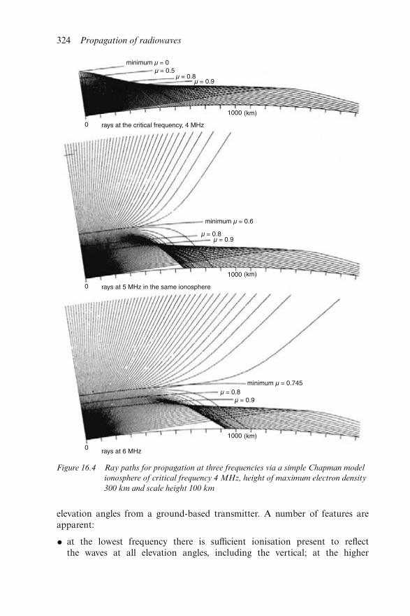
elevation angles from a ground-based transmitter. A number of features areapparent:
• at the lowest frequency there is sufficient ionisation present to reflectthe waves at all elevation angles, including the vertical; at the higher
Figure 16.4 Ray paths for propagation at three frequencies via a simple Chapman model
ionosphere of critical frequency 4 MHz, height of maximum electron density
300 km and scale height 100 km
324 Propagation of radiowaves
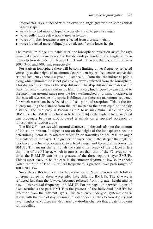
frequencies, rays launched with an elevation angle greater than some criticalvalue escape;
• waves launched more obliquely, generally, travel to greater ranges
• waves suffer more refraction at greater heights
• waves of higher frequencies are reflected from a greater height
• waves launched more obliquely are reflected from a lower height
The maximum range attainable after one ionospheric reflection arises for rayslaunched at grazing incidence and this depends primarily on the height of maxi-mum electron density. For typical E, F1 and F2 layers, the maximum range is2000, 3400 and 4000 km, respectively.
For a given ionosphere there will be some limiting upper frequency reflectedvertically at the height of maximum electron density. At frequencies above thiscritical frequency there is a ground distance out from the transmitter at pointsalong which illumination is not possible by waves reflected from the ionosphere.This distance is known as the skip distance. The skip distance increases as thewave frequency increases and in the limit for a very high frequency can extend tothe maximum ground range possible for rays launched at grazing incidence; inthat case all rays escape into space. It follows that there is a maximum frequencyfor which waves can be reflected to a fixed point of reception. This is the fre-quency making the distance from the transmitter to the point equal to the skipdistance. The frequency is known as the basic maximum usable frequency(BMUF). The BMUF is defined in Reference [16] as the highest frequency thatcan propagate between ground-based terminals on a specified occasion byionospheric refraction alone.
The BMUF increases with ground distance and depends also on the amountof ionisation present. It depends too on the height of the ionosphere since thedetermining factor as to whether reflection or transmission occurs is the angleof incidence at the layer. The greater the layer height, the steeper the angle ofincidence to achieve propagation to a fixed range, and therefore the lower theBMUF. This means that although the critical frequency of the E layer is lessthan that of the F1 layer, which in turn is less than that of the F2 layer, some-times the E-BMUF can be the greatest of the three separate layer BMUFs.This is most likely to be the case in the summer daytime at low solar epochs(when the ratio of E to F2 critical frequencies is greatest) over path ranges of1000–2000 km.
Since the earth’s field leads to the production of O and X waves which followdifferent ray paths, these waves also have differing BMUFs. The O wave isrefracted less than the X wave, becomes reflected from a greater height and sohas a lower critical frequency and BMUF. For propagation between a pair offixed terminals the path BMUF is the greatest of the individual BMUFs forreflection from the different layers. This frequency undergoes systematic vari-ations with the time of day, season and solar epoch as the electron density andlayer heights vary; there are also large day-to-day changes that create problemsfor modelling.
Ionospheric propagation 325
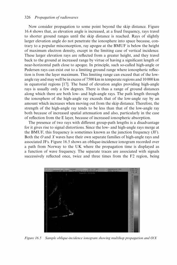
Now consider propagation to some point beyond the skip distance. Figure16.4 shows that, as elevation angle is increased, at a fixed frequency, rays travelto shorter ground ranges until the skip distance is reached. Rays of slightlylarger elevation angle do not penetrate the ionosphere into space because, con-trary to a popular misconception, ray apogee at the BMUF is below the heightof maximum electron density, except in the limiting case of vertical incidence.These larger elevation rays are reflected from a greater height, and they travelback to the ground at increased range by virtue of having a significant length ofnear-horizontal path close to apogee. In principle, such so-called high-angle orPedersen rays can exist out to a limiting ground range where ionospheric reflec-tion is from the layer maximum. This limiting range can exceed that of the low-angle ray and may well be in excess of 7500 km in temperate regions and 10 000 kmin equatorial regions [17]. The band of elevation angles providing high-anglerays is usually only a few degrees. There is thus a range of ground distancesalong which there are both low- and high-angle rays. The path length throughthe ionosphere of the high-angle ray exceeds that of the low-angle ray by anamount which increases when moving out from the skip distance. Therefore, thestrength of the high-angle ray tends to be less than that of the low-angle rayboth because of increased spatial attenuation and also, particularly in the caseof reflection from the E layer, because of increased ionospheric absorption.
The presence of two rays with different group-path lengths is a disadvantagefor it gives rise to signal distortions. Since the low- and high-angle rays merge atthe BMUF, this frequency is sometimes known as the junction frequency (JF).Both the O and X waves have their own separate families of high-angle rays andassociated JFs. Figure 16.5 shows an oblique-incidence ionogram recorded overa path from Norway to the UK where the propagation time is displayed asa function of wave frequency. The separate traces are associated with signalssuccessively reflected once, twice and three times from the F2 region, being
Figure 16.5 Sample oblique-incidence ionogram showing multihop propagation and O/X
326 Propagation of radiowaves
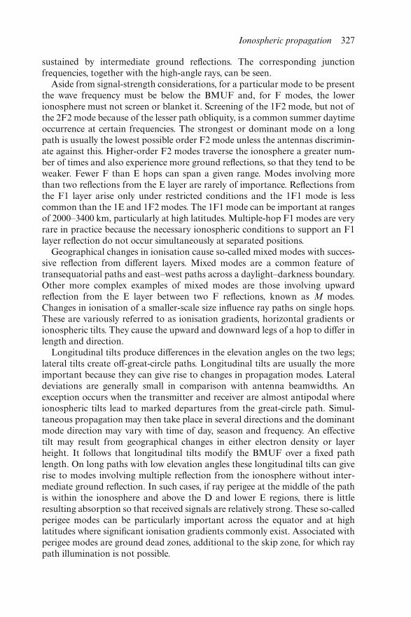
sustained by intermediate ground reflections. The corresponding junctionfrequencies, together with the high-angle rays, can be seen.
Aside from signal-strength considerations, for a particular mode to be presentthe wave frequency must be below the BMUF and, for F modes, the lowerionosphere must not screen or blanket it. Screening of the 1F2 mode, but not ofthe 2F2 mode because of the lesser path obliquity, is a common summer daytimeoccurrence at certain frequencies. The strongest or dominant mode on a longpath is usually the lowest possible order F2 mode unless the antennas discrimin-ate against this. Higher-order F2 modes traverse the ionosphere a greater num-ber of times and also experience more ground reflections, so that they tend to beweaker. Fewer F than E hops can span a given range. Modes involving morethan two reflections from the E layer are rarely of importance. Reflections fromthe F1 layer arise only under restricted conditions and the 1F1 mode is lesscommon than the 1E and 1F2 modes. The 1F1 mode can be important at rangesof 2000–3400 km, particularly at high latitudes. Multiple-hop F1 modes are veryrare in practice because the necessary ionospheric conditions to support an F1layer reflection do not occur simultaneously at separated positions.
Geographical changes in ionisation cause so-called mixed modes with succes-sive reflection from different layers. Mixed modes are a common feature oftransequatorial paths and east–west paths across a daylight–darkness boundary.Other more complex examples of mixed modes are those involving upwardreflection from the E layer between two F reflections, known as M modes.Changes in ionisation of a smaller-scale size influence ray paths on single hops.These are variously referred to as ionisation gradients, horizontal gradients orionospheric tilts. They cause the upward and downward legs of a hop to differ inlength and direction.
Longitudinal tilts produce differences in the elevation angles on the two legs;lateral tilts create off-great-circle paths. Longitudinal tilts are usually the moreimportant because they can give rise to changes in propagation modes. Lateraldeviations are generally small in comparison with antenna beamwidths. Anexception occurs when the transmitter and receiver are almost antipodal whereionospheric tilts lead to marked departures from the great-circle path. Simul-taneous propagation may then take place in several directions and the dominantmode direction may vary with time of day, season and frequency. An effectivetilt may result from geographical changes in either electron density or layerheight. It follows that longitudinal tilts modify the BMUF over a fixed pathlength. On long paths with low elevation angles these longitudinal tilts can giverise to modes involving multiple reflection from the ionosphere without inter-mediate ground reflection. In such cases, if ray perigee at the middle of the pathis within the ionosphere and above the D and lower E regions, there is littleresulting absorption so that received signals are relatively strong. These so-calledperigee modes can be particularly important across the equator and at highlatitudes where significant ionisation gradients commonly exist. Associated withperigee modes are ground dead zones, additional to the skip zone, for which raypath illumination is not possible.
Ionospheric propagation 327
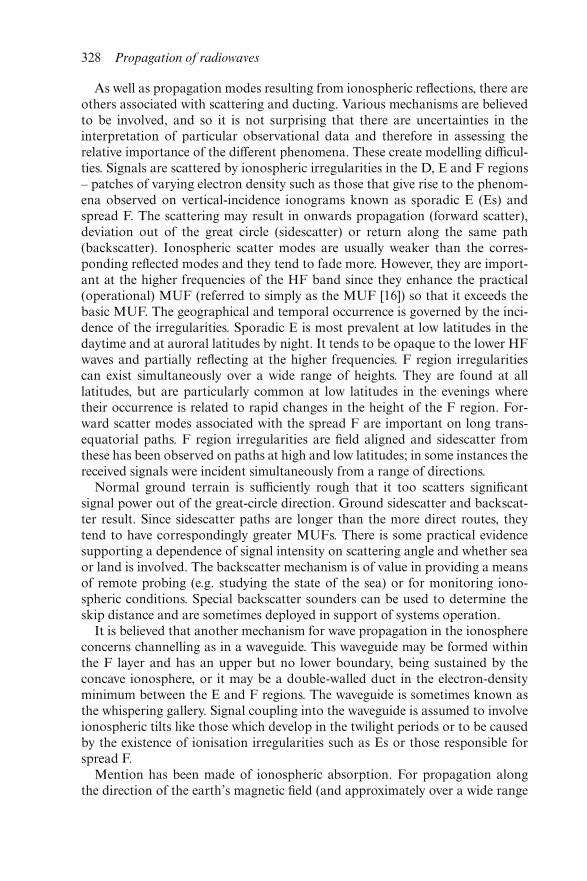
As well as propagation modes resulting from ionospheric reflections, there areothers associated with scattering and ducting. Various mechanisms are believedto be involved, and so it is not surprising that there are uncertainties in theinterpretation of particular observational data and therefore in assessing therelative importance of the different phenomena. These create modelling difficul-ties. Signals are scattered by ionospheric irregularities in the D, E and F regions– patches of varying electron density such as those that give rise to the phenom-ena observed on vertical-incidence ionograms known as sporadic E (Es) andspread F. The scattering may result in onwards propagation (forward scatter),deviation out of the great circle (sidescatter) or return along the same path(backscatter). Ionospheric scatter modes are usually weaker than the corres-ponding reflected modes and they tend to fade more. However, they are import-ant at the higher frequencies of the HF band since they enhance the practical(operational) MUF (referred to simply as the MUF [16]) so that it exceeds thebasic MUF. The geographical and temporal occurrence is governed by the inci-dence of the irregularities. Sporadic E is most prevalent at low latitudes in thedaytime and at auroral latitudes by night. It tends to be opaque to the lower HFwaves and partially reflecting at the higher frequencies. F region irregularitiescan exist simultaneously over a wide range of heights. They are found at alllatitudes, but are particularly common at low latitudes in the evenings wheretheir occurrence is related to rapid changes in the height of the F region. For-ward scatter modes associated with the spread F are important on long trans-equatorial paths. F region irregularities are field aligned and sidescatter fromthese has been observed on paths at high and low latitudes; in some instances thereceived signals were incident simultaneously from a range of directions.
Normal ground terrain is sufficiently rough that it too scatters significantsignal power out of the great-circle direction. Ground sidescatter and backscat-ter result. Since sidescatter paths are longer than the more direct routes, theytend to have correspondingly greater MUFs. There is some practical evidencesupporting a dependence of signal intensity on scattering angle and whether seaor land is involved. The backscatter mechanism is of value in providing a meansof remote probing (e.g. studying the state of the sea) or for monitoring iono-spheric conditions. Special backscatter sounders can be used to determine theskip distance and are sometimes deployed in support of systems operation.
It is believed that another mechanism for wave propagation in the ionosphereconcerns channelling as in a waveguide. This waveguide may be formed withinthe F layer and has an upper but no lower boundary, being sustained by theconcave ionosphere, or it may be a double-walled duct in the electron-densityminimum between the E and F regions. The waveguide is sometimes known asthe whispering gallery. Signal coupling into the waveguide is assumed to involveionospheric tilts like those which develop in the twilight periods or to be causedby the existence of ionisation irregularities such as Es or those responsible forspread F.
Mention has been made of ionospheric absorption. For propagation alongthe direction of the earth’s magnetic field (and approximately over a wide range
328 Propagation of radiowaves
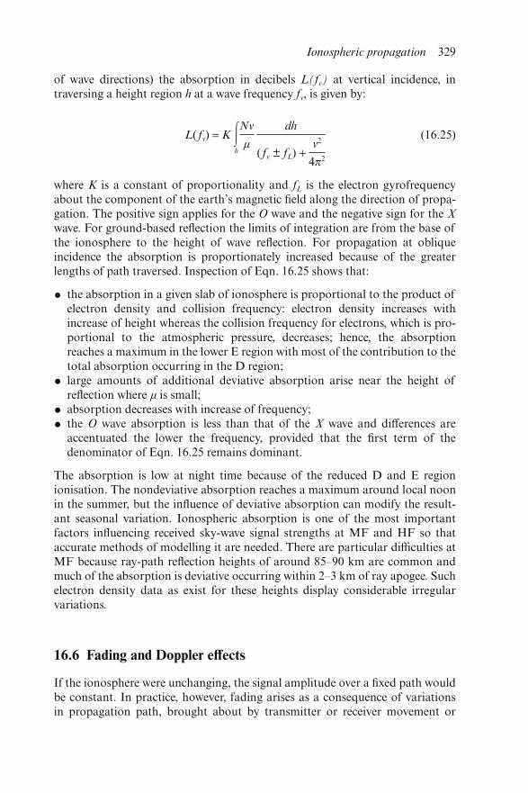
of wave directions) the absorption in decibels L(fν) at vertical incidence, intraversing a height region h at a wave frequency fν, is given by:
L( fν) = K �h
Nν
μ
dh
( fν ± fL) +ν2
4π2
(16.25)
where K is a constant of proportionality and fL is the electron gyrofrequencyabout the component of the earth’s magnetic field along the direction of propa-gation. The positive sign applies for the O wave and the negative sign for the Xwave. For ground-based reflection the limits of integration are from the base ofthe ionosphere to the height of wave reflection. For propagation at obliqueincidence the absorption is proportionately increased because of the greaterlengths of path traversed. Inspection of Eqn. 16.25 shows that:
• the absorption in a given slab of ionosphere is proportional to the product ofelectron density and collision frequency: electron density increases withincrease of height whereas the collision frequency for electrons, which is pro-portional to the atmospheric pressure, decreases; hence, the absorptionreaches a maximum in the lower E region with most of the contribution to thetotal absorption occurring in the D region;
• large amounts of additional deviative absorption arise near the height ofreflection where μ is small;
• absorption decreases with increase of frequency;
• the O wave absorption is less than that of the X wave and differences areaccentuated the lower the frequency, provided that the first term of thedenominator of Eqn. 16.25 remains dominant.
The absorption is low at night time because of the reduced D and E regionionisation. The nondeviative absorption reaches a maximum around local noonin the summer, but the influence of deviative absorption can modify the result-ant seasonal variation. Ionospheric absorption is one of the most importantfactors influencing received sky-wave signal strengths at MF and HF so thataccurate methods of modelling it are needed. There are particular difficulties atMF because ray-path reflection heights of around 85–90 km are common andmuch of the absorption is deviative occurring within 2–3 km of ray apogee. Suchelectron density data as exist for these heights display considerable irregularvariations.
16.6 Fading and Doppler effects
If the ionosphere were unchanging, the signal amplitude over a fixed path wouldbe constant. In practice, however, fading arises as a consequence of variationsin propagation path, brought about by transmitter or receiver movement or
Ionospheric propagation 329
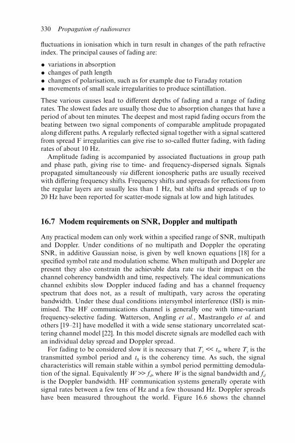
fluctuations in ionisation which in turn result in changes of the path refractiveindex. The principal causes of fading are:
• variations in absorption
• changes of path length
• changes of polarisation, such as for example due to Faraday rotation
• movements of small scale irregularities to produce scintillation.
These various causes lead to different depths of fading and a range of fadingrates. The slowest fades are usually those due to absorption changes that have aperiod of about ten minutes. The deepest and most rapid fading occurs from thebeating between two signal components of comparable amplitude propagatedalong different paths. A regularly reflected signal together with a signal scatteredfrom spread F irregularities can give rise to so-called flutter fading, with fadingrates of about 10 Hz.
Amplitude fading is accompanied by associated fluctuations in group pathand phase path, giving rise to time- and frequency-dispersed signals. Signalspropagated simultaneously via different ionospheric paths are usually receivedwith differing frequency shifts. Frequency shifts and spreads for reflections fromthe regular layers are usually less than 1 Hz, but shifts and spreads of up to20 Hz have been reported for scatter-mode signals at low and high latitudes.
16.7 Modem requirements on SNR, Doppler and multipath
Any practical modem can only work within a specified range of SNR, multipathand Doppler. Under conditions of no multipath and Doppler the operatingSNR, in additive Gaussian noise, is given by well known equations [18] for aspecified symbol rate and modulation scheme. When multipath and Doppler arepresent they also constrain the achievable data rate via their impact on thechannel coherency bandwidth and time, respectively. The ideal communicationschannel exhibits slow Doppler induced fading and has a channel frequencyspectrum that does not, as a result of multipath, vary across the operatingbandwidth. Under these dual conditions intersymbol interference (ISI) is min-imised. The HF communications channel is generally one with time-variantfrequency-selective fading. Watterson, Angling et al., Mastrangelo et al. andothers [19–21] have modelled it with a wide sense stationary uncorrelated scat-tering channel model [22]. In this model discrete signals are modelled each withan individual delay spread and Doppler spread.
For fading to be considered slow it is necessary that Ts << t0, where Ts is thetransmitted symbol period and t0 is the coherency time. As such, the signalcharacteristics will remain stable within a symbol period permitting demodula-tion of the signal. Equivalently W >> fd, where W is the signal bandwidth and fd
is the Doppler bandwidth. HF communication systems generally operate withsignal rates between a few tens of Hz and a few thousand Hz. Doppler spreadshave been measured throughout the world. Figure 16.6 shows the channel
330 Propagation of radiowaves
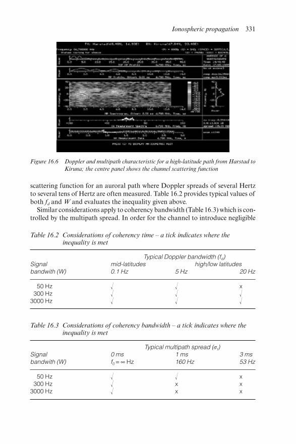
scattering function for an auroral path where Doppler spreads of several Hertzto several tens of Hertz are often measured. Table 16.2 provides typical values ofboth fd and W and evaluates the inequality given above.
Similar considerations apply to coherency bandwidth (Table 16.3) which is con-trolled by the multipath spread. In order for the channel to introduce negligible
Figure 16.6 Doppler and multipath characteristic for a high-latitude path from Harstad to
Kiruna; the centre panel shows the channel scattering function
Table 16.2 Considerations of coherency time – a tick indicates where theinequality is met
Typical Doppler bandwidth (fd)Signal mid-latitudes high/low latitudesbandwith (W) 0.1 Hz 5 Hz 20 Hz
50 Hz � � x300 Hz � � �
3000 Hz � � �
Table 16.3 Considerations of coherency bandwidth – a tick indicates where theinequality is met
Typical multipath spread (σt)Signal 0 ms 1 ms 3 msbandwith (W) f0 = ∞ Hz 160 Hz 53 Hz
50 Hz � � x300 Hz � x x
3000 Hz � x x
Ionospheric propagation 331
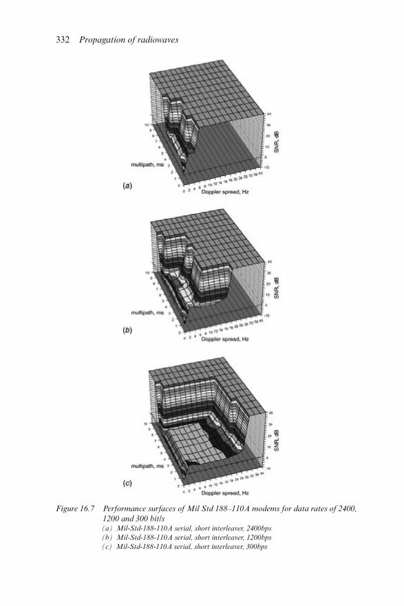
Figure 16.7 Performance surfaces of Mil Std 188–110A modems for data rates of 2400,
1200 and 300 bit/s(a) Mil-Std-188-110A serial, short interleaver, 2400bps
(b) Mil-Std-188-110A serial, short interleaver, 1200bps
(c) Mil-Std-188-110A serial, short interleaver, 300bps
332 Propagation of radiowaves
channel distortion it is necessary for f0 >> W, where f0 is the channel coherencybandwidth. In the ionospheric community we define a root mean squared(RMS) delay spread, σt and write f0 = 1/2πσt. Equivalently, we therefore require1/2πσt >> W.
Table 16.3 shows that it is difficult to achieve flat fading at anything more thanmoderate symbol rates and only low rate modems (50 to 100 baud) can operatewithout significant ISI. Conversely, Table 16.2 has demonstrated that these lowrate modems are susceptible to Doppler effects at high and low latitudes.
Historically, the issues of coherency bandwidth and coherency time limitedreliable HF digital data transmissions to mid-latitudes and even then at lowsymbol rates. However, for many applications these rates were simply unaccept-able. In order to overcome the coherency bandwidth problem multicarriermodems using a number of orthogonal carriers within the operating bandwidthwere developed, thereby keeping the symbol rate low. Adaptive channelequalisers have also been developed.
Figure 16.7 shows the performance of a standard single carrier modemoperating at different bit rates, where the surface is that combination of SNR,multipath and Doppler spread required to provide a BER of 1 in 103 whenthe Doppler shift is zero Hz. The improved operating range at lower data ratesis clear.
16.8 References
1 GOODMAN, J.M., and AARONS, J.: ‘Ionospheric effects on modernelectronic systems,’ Proc. IEEE, pp. 512–528, 78, 1990.
2 GOTT, G.F., CHAN, S.K., PANTJIAROS, C.A., and LAYCOCK, P.J.:‘High frequency spectral occupancy at the solstices’, IEE Proc. Commun.1997, 144
3 KNEPP, D.L., and HOUPIS, H.L.F.: ‘Altair VHF/UHF observations ofmultipath and backscatter enhancement’, IEEE Trans. Antennas Propag.,1991, 39, 528–534
4 BISHOP, G.J., MAZZELLA, A.J., HOLLAND, A., and RAO, S.: ‘Anoverview of ionospheric effects and mitigation in RF communication, navi-gation and surveillance’, Ionospheric effects symposium, Alexandria, USA,1996 (JMG Associates Ltd, Alexandria, VA.)
5 CANNON, P.S.: ‘Morphology of the high latitude ionosphere and itsimplications for HF communications systems,’ IEE Proc. I, 1989, 136,pp.1–10
6 NcNAMARA, L.F.: ‘The ionosphere, communications, surveillance anddirection finding’ (Krieger Publishing Company, Malabar, Florida; 1991)
7 JONES, R.M., and STEPHENSON, J.J.: ‘A three-dimensional ray tracingcomputer program for radio waves in the ionosphere’. US Dept. ofCommerce, Office of Telecommunications OT report 75–76, 1975
8 CROFT, T.A. and HOOGASIAN, H.: ‘Exact ray calculations in aquasi-parabolic ionosphere’, Radio Sci. 1968, 3, pp.69–74
9 MILSOM, J.D.: ‘Exact ray path calculations in a modified Bradley-
Ionospheric propagation 333
Dudeney model ionosphere’, IEE Proc. H, Microw. Antennas Propag. 1985,132, 33–38
10 DYSON, P. and BENNETT, J.A.: ‘A model of the vertical distribution ofthe electron concentration in the Ionosphere and its application to obliquepropagation studies’, J. Atmos. Terr. Phys. 1980, 50, pp.251–262
11 BAKER, D.C., and LAMBERT, S.: ‘Range estimation for SSL HFDF bymeans of a multi-quasi-parabolic ionospheric model’, IEE Proc. H, 1989,136, pp.120–125
12 NORMAN, R.J., and CANNON, P.S.: ‘An evaluation of a new 2-Danalytic ionospheric ray tracing technique – SMART’, Radio Sci. 1999, 34,489–499
13 NORMAN, R.J., and CANNON, P.S.: Cannon, ‘A two-dimensional ana-lytic ray tracing technique accommodating horizontal gradients’, RadioSci., 1997, 32, pp.387–396
14 BENNETT, J.A., CHEN, J., and DYSON, P.L.: ‘Analytic ray tracing for thestudy of HF magneto-ionic radio propagation in the ionosphere’, Appl.Comput. Electromagn. Soc. J., 1991, 6, pp.192–210
15 GOODMAN, J.M.: ‘HF communications science and technology’ (VanNostrand Reinhold, 1992)
16 ITU-R Recommendation P.373–7: ‘Definitions of maximum and minimumtransmission frequencies’. International Telecommunication Union,Geneva, 1995
17 CCIR Report 250–6: ‘Long-distance ionospheric propagation withoutintermediate ground reflection’, International Telecommunication Union,Geneva, 1990
18 PROAKIS, J.G.: ‘Digital communications’ (McGraw-Hill, 1989, 2nd edn.)19 WATTERSON, C.C., JUROSHEK, J.J., and BENSEMA, W.D.: ‘Experi-
mental confirmation of an HF channel model’, IEEE Trans. Commun.Technol. 1970, 18, pp.792–803
20 ANGLING, M.J., CANNON, P.C., DAVIES, N.C., WILLINK, T.J.,JODALEN, V., and LUNDBORG, B.: ‘Measurements of doppler andmultipath spread on oblique high-latitude HF paths and their use in charac-terising data modem performance’, Radio Sci. 1998, 33, pp.97–107
21 MASTRANGELO, J.F., LEMMON, J.E., VOGLER, L.E.,HOFFMEYER, J.A., PRATT, L.E., and BEHM, C.J.: ‘A new widebandhigh frequency channel simulation system’, IEEE Trans. Commun. 1997, 45,pp.26–34
22 BELLO, P.A.: ‘Characterization of randomly time variant linear channels’,IEEE Trans. Commun. Systems, 1963, 11, pp.360–393
334 Propagation of radiowaves
Chapter 17
Ionospheric prediction methods and models
Paul S. Cannon
17.1 Introduction
The ionosphere, the ionised region of the atmosphere between about 60 km and1000 km, affects all radio signals below ∼5 GHz which pass through or travel via
it. Some of the associated radio systems can only operate because of the iono-sphere, but it can also degrade radio system operation. Sometimes the effects ofthe ionosphere are highly significant, sometimes they can all but be ignored. Forhigh frequency (HF) sky-wave propagation the ionosphere is, of course, aprerequisite.
If the ionosphere were stable in time and constant in space it would be rela-tively easy to determine the effect of the ionisation on the radio propagation andhence on the radio system. Unfortunately, stability is not the norm, particularlyin the high-latitude regions [1], and as a consequence ionospheric predictionmethods and models are required to support system design, service planningand frequency management. These methods and models characterise themedium and estimate the system performance. Some operate in real, or close toreal, time and they may even directly advise the radio operator on a course ofaction which would improve system performance.
Ionospheric prediction methods can be considered to incorporate one ormore of a number of elements:
• an ionospheric model
• a ray tracing method
• system factors including antennas, noise etc.
• a calculation of the parameter(s) of interest, e.g. SNR
17.1.1 System design and service planning
A prediction method containing all four elements noted above is often used forlong-term prediction of system performance. In such cases it is usual to providemonthly median estimates of system performance at specific hours. In HFmodels ray-path and launch angle information can be obtained from the modelfor antenna optimisation. The main use of such models is, however, the calcula-tion of signal field strength and signal-to-noise ratio (SNR) at a number offrequencies. This is usually accompanied by a statistical quantification of day-to-day variability and the probability that an acceptable quality-of-service(QOS) will be met. At higher frequencies the parameter of interest might well bethe signal group delay to support the development of spaceborne navigationsystems or it might be scintillation depth to support the development of UHFsatellite communications modems.
17.1.2 Short-term adaptation to the propagation environment
Frequency management involves real-time adaptation of the operating fre-quency to optimise system operation. In many modern point-to-point HF sys-tems this is achieved using automatic link establishment (ALE) systems such asMilStd 188–141A [2] but this is not possible for broadcast systems. Further,ALE takes no account of interference, both within a network and on otherusers. Therefore, some HF users need a real-time specification of theionosphere or system performance or even a forecast of the likely situation.Likewise, a number of UHF systems require an up-to-date assessment of theionosphere. A good example of this is single-frequency operation of the globalpositioning system (GPS) when high accuracy is required. Short-term adapta-tion is, of course, far more difficult to achieve than the median prediction sinceit requires up-to-date ionospheric measurements and strategies for using thesedata.
17.2. Ionospheric models
17.2.1 Introduction
The most difficult aspect of propagation modelling is the generation of theionospheric model of the vertical distribution of electron concentration in the Eand F regions. The efficacy of a prediction or forecasting model is no better thanthe knowledge of the ionospheric electron density profile. Fortunately, therehave been substantial improvements in ionospheric modelling capabilities overthe past few years, both as a result of improved computing facilities and as aresult of improved ground-based sensors which can be used to provide real-timeupdates.
Bilitza [3,4] provides excellent summaries of the various ionospheric models.These cover electron density, temperature, ion composition, ionospheric electric
336 Propagation of radiowaves
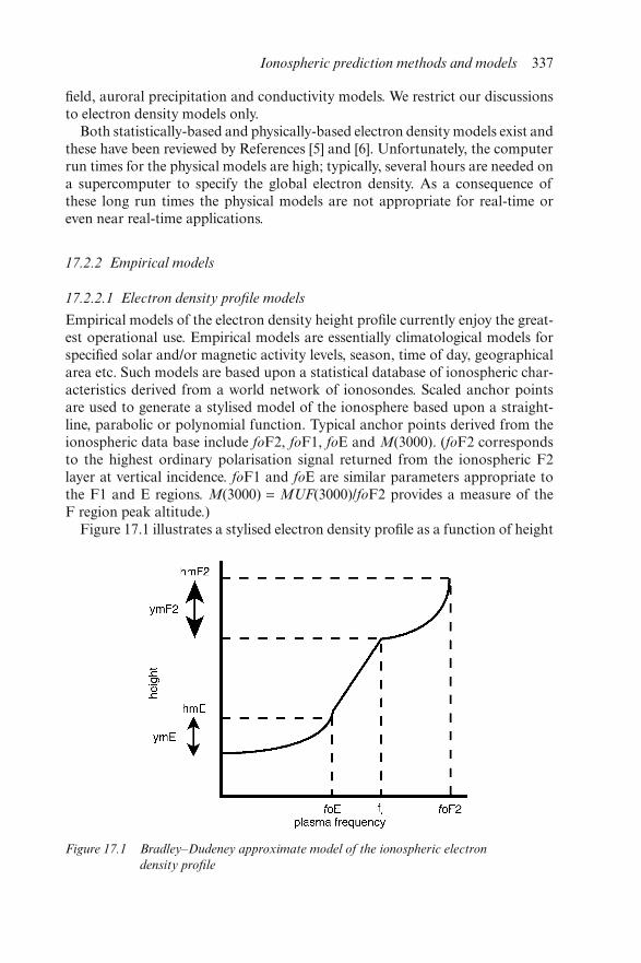
field, auroral precipitation and conductivity models. We restrict our discussionsto electron density models only.
Both statistically-based and physically-based electron density models exist andthese have been reviewed by References [5] and [6]. Unfortunately, the computerrun times for the physical models are high; typically, several hours are needed ona supercomputer to specify the global electron density. As a consequence ofthese long run times the physical models are not appropriate for real-time oreven near real-time applications.
17.2.2 Empirical models
17.2.2.1 Electron density profile models
Empirical models of the electron density height profile currently enjoy the great-est operational use. Empirical models are essentially climatological models forspecified solar and/or magnetic activity levels, season, time of day, geographicalarea etc. Such models are based upon a statistical database of ionospheric char-acteristics derived from a world network of ionosondes. Scaled anchor pointsare used to generate a stylised model of the ionosphere based upon a straight-line, parabolic or polynomial function. Typical anchor points derived from theionospheric data base include foF2, foF1, foE and M(3000). (foF2 correspondsto the highest ordinary polarisation signal returned from the ionospheric F2layer at vertical incidence. foF1 and foE are similar parameters appropriate tothe F1 and E regions. M(3000) = MUF(3000)/foF2 provides a measure of theF region peak altitude.)
Figure 17.1 illustrates a stylised electron density profile as a function of height
Figure 17.1 Bradley–Dudeney approximate model of the ionospheric electron
density profile
Ionospheric prediction methods and models 337
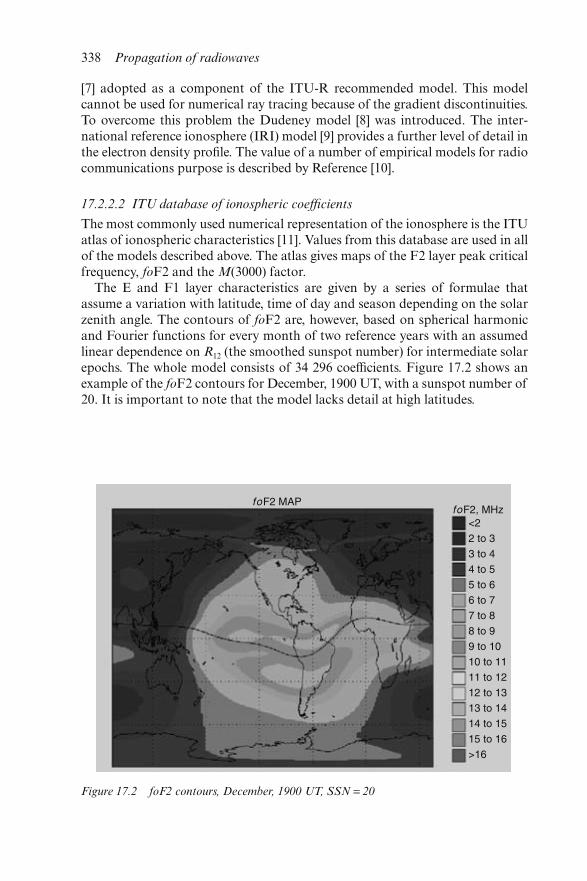
[7] adopted as a component of the ITU-R recommended model. This modelcannot be used for numerical ray tracing because of the gradient discontinuities.To overcome this problem the Dudeney model [8] was introduced. The inter-national reference ionosphere (IRI) model [9] provides a further level of detail inthe electron density profile. The value of a number of empirical models for radiocommunications purpose is described by Reference [10].
17.2.2.2 ITU database of ionospheric coefficients
The most commonly used numerical representation of the ionosphere is the ITUatlas of ionospheric characteristics [11]. Values from this database are used in allof the models described above. The atlas gives maps of the F2 layer peak criticalfrequency, foF2 and the M(3000) factor.
The E and F1 layer characteristics are given by a series of formulae thatassume a variation with latitude, time of day and season depending on the solarzenith angle. The contours of foF2 are, however, based on spherical harmonicand Fourier functions for every month of two reference years with an assumedlinear dependence on R12 (the smoothed sunspot number) for intermediate solarepochs. The whole model consists of 34 296 coefficients. Figure 17.2 shows anexample of the foF2 contours for December, 1900 UT, with a sunspot number of20. It is important to note that the model lacks detail at high latitudes.
Figure 17.2 foF2 contours, December, 1900 UT, SSN = 20
338 Propagation of radiowaves
17.2.2.3 URSI database of ionospheric coefficients
It has long been known that the ITU model is inaccurate above oceans and inthe southern hemisphere where ionosonde measurements are scarce or do notexist. Rush et al. [12,13] suggested a framework for introducing theoreticalvalues in regions of no measurements and this led to a new model which wasadopted by the International Union of Radio Science (URSI) [14].
17.2.3 Physical ionospheric models
Physical models are based on self-consistent theoretical simulations of the iono-sphere via a solution of the coupled continuity, energy and momentum equa-tions for electrons and ions. Typical input parameters required to drive themodel are the solar EUV radiation, the auroral particle precipitation (togetherwith the interaction cross sections) and the atmospheric and magnetosphericboundary conditions. From those inputs and equations the plasma densities,temperatures and drifts are obtained numerically from the nonlinear coupledsystem of equations. The value of physical models is that they can be used tounderstand the complex processes which lead to the changes in the ionosphere.For instance the coupled thermosphere ionosphere models [15,16] have beenused extensively to untangle the complex response of the ionosphere togeomagnetic storms [17,18].
17.2.4 Parameterised models
The statistical (or climatological) models and the physical models each haveadvantages and disadvantages for operational use. The accuracy of the former islimited by averaging and the rules adopted for spatial extrapolation. The secondis more intellectually appealing but the computational demands are high and themodel drivers are in reality not sufficiently well known.
A third approach is the parameterised version of the physical model. Theparameterised model begins with a physical model which gives a more realisticrepresentation of the spatial structure of the ionosphere than the statisticalmodel can provide. (Any statistical database inevitably averages over similargeophysical conditions resulting in a smoothed model which is unrepresentativeof the instantaneous ionosphere.) The physical model is then parameterised interms of solar and geographical parameters to provide an easy to use and quickto run ionospheric model.
17.2.4.1 PIM
The PIM (parameterised ionospheric model) [19] uses either the foF2 ITU coef-ficients for normalisation of the electron density profiles or it uses coefficientsproduced by a Utah State University model. The calculation of the electrondensity profile is based upon the underlying neutral composition, temperatureand wind together with electric field distributions, auroral precipitation and the
Ionospheric prediction methods and models 339
solar EUV spectrum. Inputs to the model consist of universal time and the dailyvalue of F10.7 (the solar flux at a wavelength of 10.7 cm) or the solar sunspotnumber. The current value of Kp (the index of geomagnetic activity) is alsorequired together with the sign (positive or negative) of the interplanetarymagnetic field y component. This latter factor is used to select one, of two,solar-wind-driven transport (convection) patterns in the high latitude region.The PIM model is at its most powerful, however, when it is adjusted by real timeinput data.
17.3 Prediction methods
17.3.1 HF
Prediction method development has largely followed the evolution of the iono-spheric model and more recently the development of analytic ray tracing. HFpropagation methods are in fact not new, but date back to World War II.Through the years a large number of methods have been developed and are stillbeing developed. Many are, however, not generally available and, of course, anumber have fallen into disuse because of the availability of the newer models.As a consequence this Chapter will restrict itself to a small number of the mostpopular and accessible models:
IONCAP [20]: this very popular program developed by the Institute for Tele-communications Sciences (ITS) in the USA will run on a variety of computerplatforms. A number of user friendly front ends have also been developed, forexample the derivative VOACAP [21] which also makes a number of smallchanges to the calculations used in IONCAP. IONCAP and its derivatives usevirtual mirror techniques.
ITU REC533 [22]: this is the method recommended by the International Tele-communication Union. It is a relatively simple technique but tests show that itsaccuracy is comparable to that provided by more complex methods.
ICEPAC [23]: the ionospheric communications enhanced profile analysis andcircuit (ICEPAC) prediction method is the latest program from ITS. It uses theICED electron density model which should give improved performance in thehigh latitude regions.
17.3.1.1 ICEPAC
ICEPAC represents one of the newest of the HF prediction decision aids and assuch it is worthy of more detailed discussion. Its outputs are very similar toIONCAP and it provides in total 29 different output options. The BMUF isassumed to follow a given distribution so that it is possible to determine, for eachwave frequency and mode, the fraction of days for which that mode exists – thisis known as the availability. Reference values also exist for the upper and lowerstandard deviations of the day-to-day signal variability to estimate theprobability that the signal strength will exceed a prescribed threshold.
340 Propagation of radiowaves
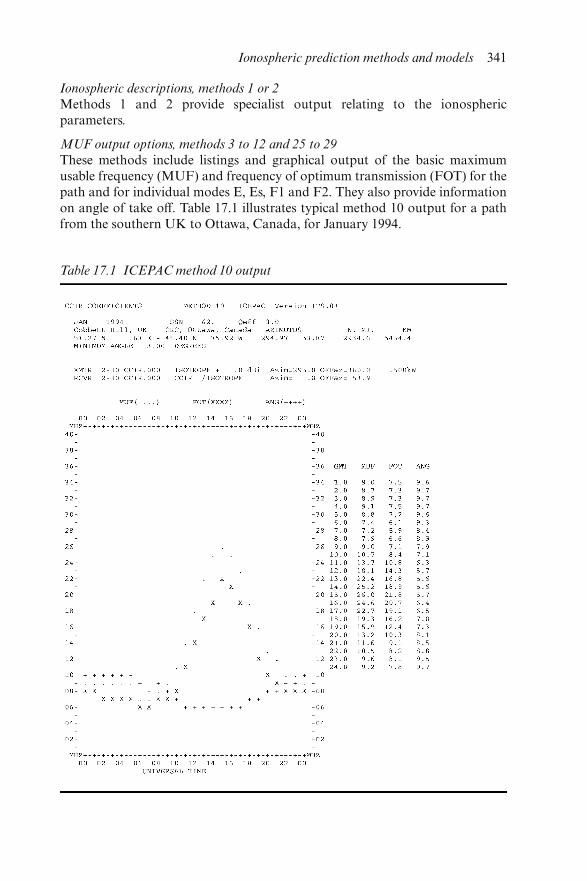
Ionospheric descriptions, methods 1 or 2
Methods 1 and 2 provide specialist output relating to the ionosphericparameters.
MUF output options, methods 3 to 12 and 25 to 29
These methods include listings and graphical output of the basic maximumusable frequency (MUF) and frequency of optimum transmission (FOT) for thepath and for individual modes E, Es, F1 and F2. They also provide informationon angle of take off. Table 17.1 illustrates typical method 10 output for a pathfrom the southern UK to Ottawa, Canada, for January 1994.
Table 17.1 ICEPAC method 10 output
Ionospheric prediction methods and models 341
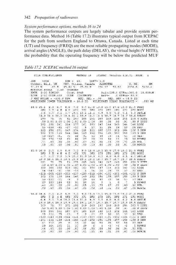
System performance options, methods 16 to 24
The system performance outputs are largely tabular and provide system per-formance data. Method 16 (Table 17.2) illustrates typical output from ICEPACfor the path from southern England to Ottawa, Canada. Listed at each time(UT) and frequency (FREQ) are the most reliable propagating modes (MODE),arrival angles (ANGLE), the path delay (DELAY), the virtual height (V HITE),the probability that the operating frequency will be below the predicted MUF
Table 17.2 ICEPAC method 16 output
342 Propagation of radiowaves
(F DAYS), the median system loss in decibels (LOSS), field strength in dBμV m−1
(DBU), median signal and noise powers at the receiver input terminals in dBw (SDBW and N DBW), signal-to-noise ratio (SNR), the required combination oftransmitter power and antenna gains needed to achieve the required reliability indecibels (RPWG), reliability, i.e. the probability that the SNR exceeds therequired SNR (REL), and the probability of an additional mode within themultipath tolerances (MPROB).
Antenna output options, methods 13 to 15
ICEPAC includes the antenna gain description of a number of antennas thatmay be specified at the transmitter and receiver. These antennas include theisotropic reference radiator, dipoles, rhombics and sloping-V antennas. Theradiation pattern of the antennas can be plotted and the effects of the antennason the system performance evaluated via methods 16 to 24.
17.3.2 Computerised models of ionospheric scintillation
The regions of ionospheric scintillation consist of a belt 20° wide centred on thegeomagnetic equator and in the polar regions above 55° to 60° latitude. Withinthe equatorial scintillation belt, Rayleigh distributed scintillation is often experi-enced at frequencies in the VHF and UHF bands during the late evening andearly morning hours from about 2000 to 0200 local time (LT). In the polarregions the scintillation is more irregular and can occur any time of day andnight although at lower levels than equatorial scintillation.
The climatology of scintillation in the equatorial regions is reasonably wellestablished and long-term average scintillation conditions in particular geo-graphic regions can be modelled using the WBMOD computer programme[25, 26]. This model also includes a climatological model of the high latitude;however this is less rigorous.
The electron density irregularities model, EDIM, within WBMOD is a collec-tion of empirical models which describe the geometry, orientation, strength andmotion of the irregularities as a function of latitude, date, time of day, solaractivity and geomagnetic activity.
One of the basic parameters generated by the model is the height-integratedelectron density irregularity strength, CkL, which is a measure of the verticalheight integrated power in the irregularities. It is this parameter which is mostdynamic and controls the worldwide scintillation.
The propagation model implemented in WBMOD is that described by Rino[27]. This model assumes that all propagation is line-of-sight, and that the scin-tillation effects can be calculated as though the effect of the ionosphericirregularities can be ascribed to an infinitely thin, phase-changing screen set atsome altitude within the irregularity layer. A propagating ray passing throughthe screen will have its phase changed according to the spectral characteristics ofthe irregularities, and the resulting intensity and phase scintillation will developas the ray propagates beyond the screen to the receiver. The irregularities are
Ionospheric prediction methods and models 343
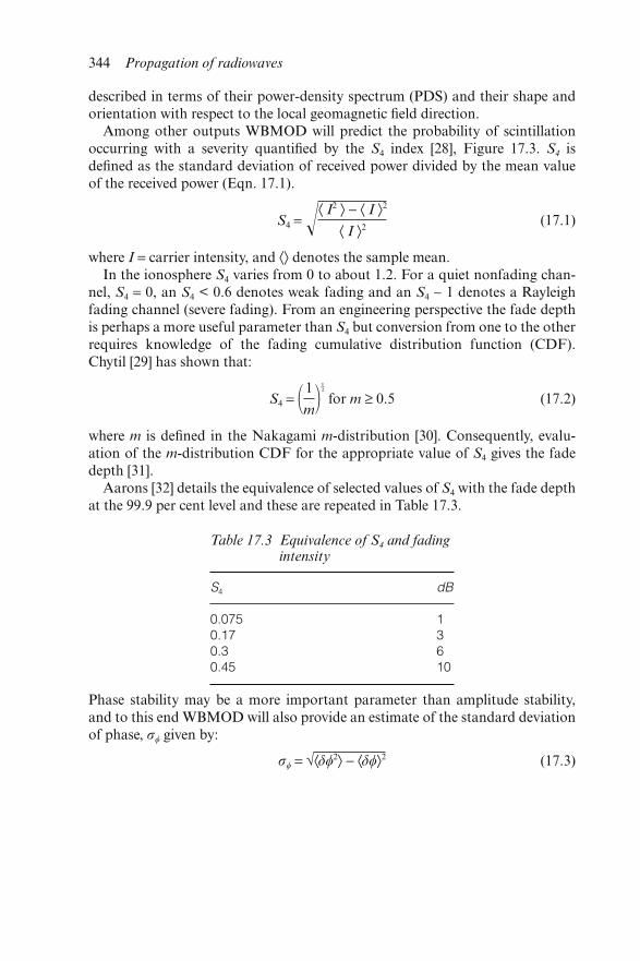
described in terms of their power-density spectrum (PDS) and their shape andorientation with respect to the local geomagnetic field direction.
Among other outputs WBMOD will predict the probability of scintillationoccurring with a severity quantified by the S4 index [28], Figure 17.3. S4 isdefined as the standard deviation of received power divided by the mean valueof the received power (Eqn. 17.1).
S4 = �⟨ I2 ⟩ − ⟨ I ⟩2
⟨ I ⟩2(17.1)
where I = carrier intensity, and ⟨⟩ denotes the sample mean.In the ionosphere S4 varies from 0 to about 1.2. For a quiet nonfading chan-
nel, S4 = 0, an S4 < 0.6 denotes weak fading and an S4 ∼ 1 denotes a Rayleighfading channel (severe fading). From an engineering perspective the fade depthis perhaps a more useful parameter than S4 but conversion from one to the otherrequires knowledge of the fading cumulative distribution function (CDF).Chytil [29] has shown that:
S4 = �1
m�–¹² for m ≥ 0.5 (17.2)
where m is defined in the Nakagami m-distribution [30]. Consequently, evalu-ation of the m-distribution CDF for the appropriate value of S4 gives the fadedepth [31].
Aarons [32] details the equivalence of selected values of S4 with the fade depthat the 99.9 per cent level and these are repeated in Table 17.3.
Phase stability may be a more important parameter than amplitude stability,and to this end WBMOD will also provide an estimate of the standard deviationof phase, σ given by:
σ = √⟨δ2⟩ − ⟨δ⟩2 (17.3)
Table 17.3 Equivalence of S4 and fadingintensity
S4 dB
0.075 10.17 30.3 60.45 10
344 Propagation of radiowaves
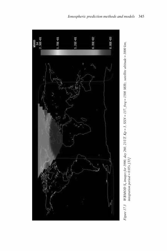
Fig
ure
17.3
WB
MO
D S
4 i
mage
s fo
r 1990,
day 2
60,
21U
T,
Kp =
3,
SS
N =
137,
freq
= 1
500 M
Hz,
sate
llit
e alt
itude
= 1000 k
m,
inte
gra
tion p
erio
d =
0.0
5s
[33]
Ionospheric prediction methods and models 345
17.4 Application specific models
The aforementioned propagation models exhibit a general architecture whichmakes them useful in many applications. A number of prediction methods have,however, been developed which take these generalised architectures and developthem for specific applications.
In military HF, low probability of interception/jamming (LPI/LPJ) is import-ant and is generally based on techniques such as spread spectrum, cryptographyand antenna nulling. Even with such sophisticated strategies the signals can stillpropagate to unwanted or unauthorised receivers causing interference or result-ing in the transmission of intelligence. An alternative technique, based on thetactical use of signal propagation prediction [34,35], may then be advantageous.The tactical technique exploits detailed knowledge of the ionosphere and raytracing to minimise the signal coverage and thereby deny, or minimise, the hos-tile receiver’s access to the radiated electromagnetic energy. The technique canbe used in isolation or in conjunction with more sophisticated LPI/LPJtechniques.
Although this tactical technique could be performed using any of a numberof current prediction programs it is operator intensive, specialist data (e.g. loca-tion of interceptors and frequency plans) are required and the contribution fromthe ground wave may not be assessed.
To overcome these deficiencies tactical HF decision aids have been developed.An example is the HF electromagnetic environmental modelling system (HF–EEMS)[36]. The aid is designed to enable both HF experts and inexperiencedoperators to predict those communications system parameters such as fre-quency, receiver station and radiated power which optimise the HF system. Thedecision aid uses a modified version of the REC533 prediction program [21].HF–EEMS V1.1 also contains a simple ground-wave propagation model forline-of-sight (LOS < 200 km) systems. The ground-wave propagation character-istics are calculated by a modified version of GRWAVE [37], which computesground wave field strengths over a smooth, curved, homogeneous earth.
The decision aid displays data to the operator in two formats: signal coveragemaps and frequency tables. In Figure 17.4 both the sky-wave and ground-wavesignals (the latter as concentric circles) are shown on the same map, along withfriendly and hostile station locations. These monthly median maps enable usersto inspect communications link configurations and evaluate the effectiveness ofbroadcast transmissions.
Via a table, the decision aid also recommends the best operating frequenciesto minimise hostile interception. There are two approaches which can beemployed, one based on LUF (lowest usable frequency) considerations and theother based upon the MUF. In the former the aim is to operate on a frequencywhich is below the LUF to the hostile receivers but above the LUF to thefriendly receivers. The latter approach aims to choose a frequency which is abovethe MUF to the hostile receivers but below the MUF to the friendly receivers. Itis to be noted that the LUF technique is more problematical since it relies on
346 Propagation of radiowaves
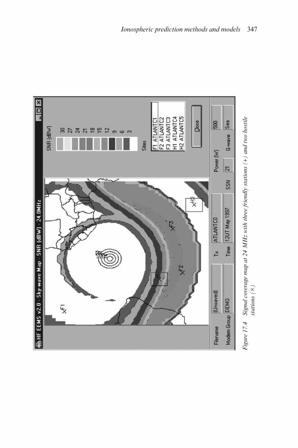
Fig
ure
17.4
Sig
nal
cove
rage
map a
t 24 M
Hz
wit
h t
hre
e fr
iendly
sta
tions
(+)
and t
wo h
ost
ile
stati
ons
(×
)
Ionospheric prediction methods and models 347
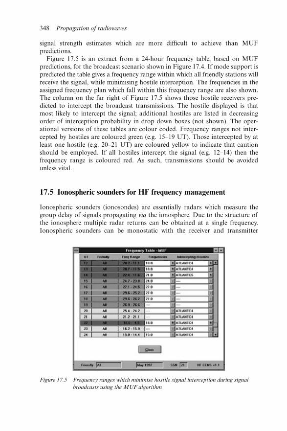
signal strength estimates which are more difficult to achieve than MUFpredictions.
Figure 17.5 is an extract from a 24-hour frequency table, based on MUFpredictions, for the broadcast scenario shown in Figure 17.4. If mode support ispredicted the table gives a frequency range within which all friendly stations willreceive the signal, while minimising hostile interception. The frequencies in theassigned frequency plan which fall within this frequency range are also shown.The column on the far right of Figure 17.5 shows those hostile receivers pre-dicted to intercept the broadcast transmissions. The hostile displayed is thatmost likely to intercept the signal; additional hostiles are listed in decreasingorder of interception probability in drop down boxes (not shown). The oper-ational versions of these tables are colour coded. Frequency ranges not inter-cepted by hostiles are coloured green (e.g. 15–19 UT). Those intercepted by atleast one hostile (e.g. 20–21 UT) are coloured yellow to indicate that cautionshould be employed. If all hostiles intercept the signal (e.g. 12–14) then thefrequency range is coloured red. As such, transmissions should be avoidedunless vital.
17.5 Ionospheric sounders for HF frequency management
Ionospheric sounders (ionosondes) are essentially radars which measure thegroup delay of signals propagating via the ionosphere. Due to the structure ofthe ionosphere multiple radar returns can be obtained at a single frequency.Ionospheric sounders can be monostatic with the receiver and transmitter
Figure 17.5 Frequency ranges which minimise hostile signal interception during signal
broadcasts using the MUF algorithm
348 Propagation of radiowaves
colocated or they can be bistatic with the transmitter and receiver separated bymany tens, hundreds or thousands of kilometres. The former generates verticalionograms and the latter oblique ionograms.
The oblique sounder provides ionospheric information such as propagatingfrequencies and multipath over the path from the sounder transmitter to thesounder receiver. If the HF communications is over the same path as thesounder, the latter provides an invaluable decision aid to choose the correctoperating frequency.
17.6 Real-time updates to models, ionospheric specificationand forecasting
17.6.1 Introduction
The performance of a wide variety of communications, surveillance, trackingand navigation systems is controlled by the ionosphere. Empirical models of thenonauroral, quiet ionosphere typically describe the median monthly or seasonalconditions at every hour. Day to day foF2 deviations from these median valuescan range from 10 to 30 per cent even for quiet magnetic conditions and willbe higher still during ionospheric storms. Furthermore, there are short-termvariations due to atmospheric gravity waves which typically have periods of 10–120 minutes. The difference between monthly median predicted and measuredsignal strengths can be up to 40 dB. These variations average out over a periodof a month or so and consequently we can use the median ionospheric modelsfor planning and certain other purposes.
However, there are circumstances where it is necessary to be able to correct forthese temporal variations in real time. Empirical or climatological models (suchas those used in the aforementioned REC533 and ICEPAC) are inadequate forthe specifications and forecasts required by many modern operational systems.We need both an ionospheric model capable of assimilating the necessary dataand also the appropriate data streams.
The most important developments in this field derive from the USA in sup-port of the Air Force Space Forecast Center (AFSFC). Both the ICED and PIMmodels were conceived to allow for real-time updates of the input parametersfrom a number of sensors. ICED updates are based only on changes of aneffective sunspot number SSNeff together with the auroral Q index whereas real-time control of PIM, via the model known as PRISM (parameterised real-timeionospheric specification model), is more sophisticated.
17.6.2 PRISM
An example of this emerging capability is the on-going development of theparameterised real-time ionospheric specification model (PRISM), now opera-tional at the U.S. Air Force Space Forecast Centre [19]. It is a parameterised
Ionospheric prediction methods and models 349
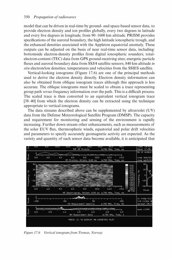
model that can be driven in real-time by ground- and space-based sensor data, toprovide electron density and ion profiles globally, every two degrees in latitudeand every five degrees in longitude, from 90–1600 km altitude. PRISM providesspecifications of the auroral boundary, the high latitude ionospheric trough, andthe enhanced densities associated with the Appleton equatorial anomaly. Theseoutputs can be adjusted on the basis of near real-time sensor data, including:bottomside electron-density profiles from digital ionospheric sounders; total-electron-content (TEC) data from GPS ground-receiving sites; energetic particlefluxes and auroral boundary data from SSJ/4 satellite sensors; 840 km altitude insitu electron/ion densities; temperatures and velocities from the SSIES satellite.
Vertical-looking ionograms (Figure 17.6) are one of the principal methodsused to derive the electron density directly. Electron density information canalso be obtained from oblique ionogram traces although this approach is lessaccurate. The oblique ionograms must be scaled to obtain a trace representinggroup path versus frequency information over the path. This is a difficult process.The scaled trace is then converted to an equivalent vertical ionogram trace[38–40] from which the electron density can be extracted using the techniqueappropriate to vertical ionograms.
The data streams described above can be supplemented by ultraviolet (UV)data from the Defense Meteorological Satellite Program (DMSP). The capacityand requirement for monitoring and sensing of the environment is rapidlyincreasing. Further down stream other enhancements, such as measurements ofthe solar EUV flux, thermospheric winds, equatorial and polar drift velocitiesand parameters to specify accurately geomagnetic activity are expected. As thevariety and quantity of such sensor data become available, it is anticipated that
Figure 17.6 Vertical ionogram from Tromsø, Norway
350 Propagation of radiowaves
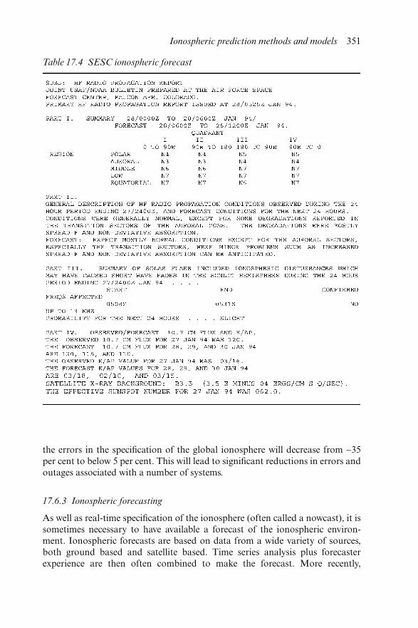
the errors in the specification of the global ionosphere will decrease from ∼35per cent to below 5 per cent. This will lead to significant reductions in errors andoutages associated with a number of systems.
17.6.3 Ionospheric forecasting
As well as real-time specification of the ionosphere (often called a nowcast), it issometimes necessary to have available a forecast of the ionospheric environ-ment. Ionospheric forecasts are based on data from a wide variety of sources,both ground based and satellite based. Time series analysis plus forecasterexperience are then often combined to make the forecast. More recently,
Table 17.4 SESC ionospheric forecast
Ionospheric prediction methods and models 351
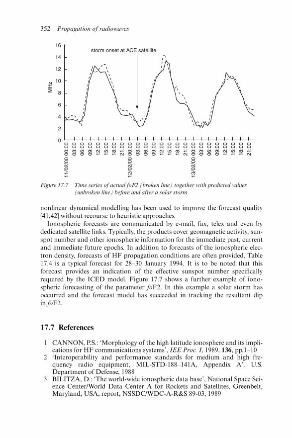
nonlinear dynamical modelling has been used to improve the forecast quality[41,42] without recourse to heuristic approaches.
Ionospheric forecasts are communicated by e-mail, fax, telex and even bydedicated satellite links. Typically, the products cover geomagnetic activity, sun-spot number and other ionospheric information for the immediate past, currentand immediate future epochs. In addition to forecasts of the ionospheric elec-tron density, forecasts of HF propagation conditions are often provided. Table17.4 is a typical forecast for 28–30 January 1994. It is to be noted that thisforecast provides an indication of the effective sunspot number specificallyrequired by the ICED model. Figure 17.7 shows a further example of iono-spheric forecasting of the parameter foF2. In this example a solar storm hasoccurred and the forecast model has succeeded in tracking the resultant dipin foF2.
17.7 References
1 CANNON, P.S.: ‘Morphology of the high latitude ionosphere and its impli-cations for HF communications systems’, IEE Proc. I, 1989, 136, pp.1–10
2 ‘Interoperability and performance standards for medium and high fre-quency radio equipment, MIL-STD-188–141A, Appendix A’. U.S.Department of Defense, 1988
3 BILITZA, D.: ‘The world-wide ionospheric data base’, National Space Sci-ence Center/World Data Center A for Rockets and Satellites, Greenbelt,Maryland, USA, report, NSSDC/WDC-A-R&S 89-03, 1989
Figure 17.7 Time series of actual foF2 (broken line) together with predicted values
(unbroken line) before and after a solar storm
352 Propagation of radiowaves
4 BILITZA, D.: ‘Solar-terrestrial models and application software’, NationalSpace Sciences Data Center, World Data Center A for Rockets and Satel-lites, Goddard Space Flight Center, Greenbelt, Maryland, USA, reportNSSDC/WDC-A-R&S 90-19, 1990
5 RUSH, C.M.: ‘Ionospheric radio propagation models and predictions – amini-review’, IEEE Trans. Antennas and Propag., 1986, 34, pp.1163–1170
6 SCHUNK, R.W. and SZUSZCZEWICZ, E.P.: ‘First principal and empiri-cal modelling of the global scale ionosphere’, Ann. Geophys., 1988, 6,pp.19–30
7 BRADLEY, P.A. and DUDENEY, J.R.: ‘A simplified model of the verticaldistribution of electron concentration in the ionosphere’, J. Atmos. Terr.Phys., 1973, 35, pp.2131–2146
8 DUDENEY, J.R.: ‘An improved model of electron concentration withheight in the ionosphere’, J. Atmos. Terr. Phys., 1983, 45, pp.629–640
9 RAWER, K. and BILITZA, D.: ‘International reference ionosphere –plasma densities: status 1988’, Adv. Space Res., 1990, 10, pp.5–14
10 DUDENEY, J.R. and KRESSMAN, R.I.: ‘Empirical models of theelectron concentration of the ionosphere and their value for radio com-munications purposes’, Radio Sci., 1986, 21, pp.319–330
11 ITU-R Recommendation P.1239: ‘ITU-R reference ionospheric charac-teristics and methods for basic MUF, operational MUF and ray-pathpredictions’, 1997
12 RUSH, C.M., POKEMPNER, M., ANDERSON, DN., STEWART, F.G.,and PERRY, J.: ‘Improving ionospheric maps using theoretically derivedvalues of foF2’, Radio Sci., 1983, 18, pp.95–107
13 RUSH, C.M., POKEMPNER, M., ANDERSON, D.N., STEWART, F.G.,and REASONER, R.: ‘Maps of FoF2 derived from observations and the-oretical data’, Radio Sci. 1984, 19, pp.1083–1097
14 FOX, M.W. and MCNAMARA, L.F.: ‘Improved empirical world maps ofFoF2:1. the method’, Ionospheric Prediction Service, Sydney, AustraliaTechnical Report IPS-TR-86-03, 1986
15 FULLER-ROWELL, T.J., REES, D., QUEGAN, S., MOFFETT, R.J.,CODRESCU, M.V., and MILLWARD, G.H.: ‘A coupled thermosphereionosphere model (CTIM)’, in SCHUNK, R.W. (Ed.): ‘Handbook ofionospheric models’, STEP Report, 1996
16 ROBLE, R.G.: ‘The NCAR thermosphere-ionosphere-mesosphere-electrodynamics general circulation model’, in SCHUNK, R.W. ‘Handbookof ionospheric models’, STEP Report, 1996
17 BURNS, A.G., KILLEEN, T.L., DENG, W., and CARIGNAN, D.R.G.:‘Geomagnetic storm effects in the low to mid latitude upper thermosphere’,J. Geophys. Res., 1995, 100, pp.14673–14691
18 FULLER-ROWELL, T.J., CODRESCU, M.V., MOFFETT, R.J., andQUEGAN, S.: ‘On the seasonal response of the thermosphere and iono-sphere to geomagnetic storms’, J. Geophys. Res, 1996, 101, pp.2343–2353
19 DANIELL, R.E., BROWN, L.D., ANDERSON, D.N., FOX, M.W.,DOHERTY, P.H., DECKER, D.T., SOJKA, J.J., and SCHUNK, R.W.:‘PRISM: a global ionospheric parameterisation based on first principlesmodels’, Radio Sci, 1995, 30, p.1499
20 TETERS, L.R., LLOYD, J.L., HAYDON, G.W., and LUCUS, D.L:
Ionospheric prediction methods and models 353
‘Estimating the performance of telecommunications systems using theionospheric transmission channel: ionospheric communications analysisand prediction program (IONCAP) user’s manual’, NTIA, Springfield, VA,USA, 1993, report 83-127, NTIS order no N70-24144
21 LANE, G., RHOADS, F.J., and DEBLASIO, L.: ‘Voice of America cover-age analysis program, (VOACAP). A guide to VOACAP’. US InformationAgency, Bureau of Broadcasting, Washington, D.C. 20547-0001, 1993, B/ESA technical report 01-93
22 ITU-R Recommendation P.533–6: ‘HF Propagation Prediction Method’,1999
23 STEWART, F.G. and HAND, G.: ‘Technical description of the ICEPACpropagation prediction program’. Institution of TelecommunicationsSciences, Boulder, Colorado, USA, 1994, private communication
24 TASCIONE, T.F., KROEHL, H.W., CREIGER, R., J.W. FREEMANJNR, WOLF, R.A., SPIRO, R.W., HILMER, R.V., SHADE, J.W., andHAUSMAN, B.A.: ‘New ionospheric and magnetospheric specificationmodels’, Radio Sci., 1988, 23, pp.211–222
25 SECAN, J.A., BUSSEY, R.M., and FREMOUW, E.J.: ‘High latitudeupgrade to the Wideband ionospheric scintillation model’, Radio Sci., 1997,32, pp.1567–1574
26 SECAN, J.A., BUSSEY, R.M., FREMOUW, E.J., and BASU, S.: ‘Animproved model of equatorial scintillation’, Radio Sci., 1995, 30, pp.607–617
27 RINO, C.L.: ‘A power law phase screen model for ionospheric scintillation,1 Weak scatter’, Radio Sci., 14, pp.1135–1145
28 BRIGGS, B.H. and PARKIN, I.A.: ‘On the variation of radio star andsatellite scintillations with zenith angle’, J. Atmos. Terr. Phys., 1963, 25,pp.339–366
29 CHYTIL, B.: ‘The distribution of amplitude scintillation and the conver-sion of scintillation indices’, J. Atmos. Terr. Phys., 1967, 29, pp.1175–1177
30 NAKAGAMI, M.: ‘Statistical methods’, in ‘Radio wave propagation’,HOFFMAN, W.C. (Ed.) (Pergamon, 1960) pp.3–36
31 WHITNEY, H.E., AARONS, J., ALLEN, R.S., and SEEMAN, D.R.:‘Estimation of the cumulative amplitude probability distribution functionof ionospheric scintillations’, Radio Sci. 1972, 7, pp.1095–1104
32 AARONS, J.: ‘Global morphology of ionospheric scintillation’, Proc.IEEE, 1982, 70, pp.360–377
33 HILMER, R.V.: ‘AF-GEOSpace user’s manual, Version 1.4 and 1.4P’ Tech.report AFRL-VS-TR-1999-1551. Hanscom AFB, MA, USA: AirForceResearch Laboratories, 1999
34 ARGO and ROTHMULLER: ‘PROPHET; an application of propagationforecasting principles’. Presented at Solar-terrestrial predictions workshopproc., 1979
35 GOODMAN, J.M., UFFELMAN, D.R., and FAHLSING, F.: ‘The role ofthe propagation environment in HF electronic warfare’. Presented at Propa-gation effects on ECM-resistant systems in communications and navigation,NATO-AGARD Electromagnetic Wave Propagation Panel, ConferenceNo. CP331, London, UK, 1982
36 SHUKLA, A.K., CANNON, P.S., ROBERTS, S., and LYNCH, D.: ‘Atactical HF decision aid for inexperienced operators and automated
354 Propagation of radiowaves
HF systems’, Presented at IEE 7th international conference on HF, radiosystems and techniques, Nottingham, UK, 1997, pp.383–387
37 ITU-R Recommendation P.386: ‘Groundwave propagation curves forfrequencies between 10 kHz and 30 MHz’, 1999
38 REILLY, M.H.: ‘Ionospheric true height profiles from oblique ionograms’,Radio Sci. 20, p.280–286
39 REILLY, M.H.: ‘A method for real height analysis of oblique ionograms’,Radio Sci. 1989, 24, pp.575–583
40 HEATON, J.A., CANNON, P.S., ROGERS, N.C., MITCHELL, C.N., andKERSLEY, L.: ‘Validation of electron density profiles derived from obliqueionograms over the UK’, Radio Sci., 36.5, p.149, 2001
41 FRANCIS, N.M., CANNON, P.S., BROWN, A.G., and BROOMHEAD,D.S.: ‘Nonlinear prediction of the ionospheric parameter foF2 on hourly,daily and monthly timescales’, J. Geophys. Res., 2000, 105, pp.12839–12849FRANCIS, N.M., BROWN, A.G., CANNON, P.S., and BROOMHEAD,D.S.: ‘Non-linear prediction of the hourly foF2 time series in conjunctionwith the interpolation of missing data points’, Phys. Chem. Earth, 2000, 25,pp.261–265
Ionospheric prediction methods and models 355

Chapter 18
Surface waves, and sky waves below 2 MHz
John Milsom
18.1 Introduction
The principal modes of radiowave propagation at frequencies below 2 MHz arethe surface wave and sky wave. In this Chapter these two modes are introducedand described. Rather than concentrate on the details of elaborate path-loss prediction theories, they are merely introduced and the discussion thenconcentrates on their application by the planning engineer.
The sky-wave propagation prediction methods described in this Chapter areonly applicable at frequencies below 2 MHz. However, the surface-wave modelsare based on more general theories and can also be applied in the HF band.
Antenna and external-noise aspects of system planning are discussed.Throughout, readers are directed towards relevant data sources, prediction
procedures and computer programs so that they might apply the planningmethods described.
18.2 Applications
The radio spectrum below 2 MHz is allocated to a variety of radio systems:
aeronautical radionavigationamateurfixed servicesland mobilemaritime mobile coastal radiotelegraphymaritime radionavigation (radio beacons)mobile (distress and calling)radiolocationradionavigation
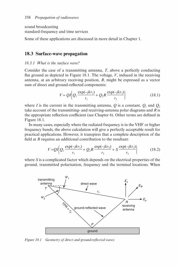
sound broadcastingstandard-frequency and time services
Some of these applications are discussed in more detail in Chapter 1.
18.3 Surface-wave propagation
18.3.1 What is the surface wave?
Consider the case of a transmitting antenna, T, above a perfectly conductingflat ground as depicted in Figure 18.1. The voltage, V, induced in the receivingantenna, at an arbitrary receiving position, R, might be expressed as a vectorsum of direct and ground-reflected components:
V = QI�Q1 exp(−jkr1)
r1
+ Q2Rexp(−jkr2)
r2� (18.1)
where I is the current in the transmitting antenna, Q is a constant, Q1 and Q2
take account of the transmitting- and receiving-antenna polar diagrams and R isthe appropriate reflection coefficient (see Chapter 6). Other terms are defined inFigure 18.1.
In many cases, especially where the radiated frequency is in the VHF or higherfrequency bands, the above calculation will give a perfectly acceptable result forpractical applications. However, it transpires that a complete description of thefield at R requires an additional contribution to the resultant:
V =QI�Q1
exp(−jkr1)
r1
+ Q2Rexp(−jkr2)
r2
+ Sexp(−jkr2)
r2� (18.2)
where S is a complicated factor which depends on the electrical properties of theground, transmitted polarisation, frequency and the terminal locations. When
Figure 18.1 Geometry of direct and ground-reflected waves
358 Propagation of radiowaves
introduced in this way, as an apparent afterthought to make up the numbers andsatisfy Maxwell’s equations, one is tempted to regard it as a minor contributionof interest primarily to the mathematical physicist. In fact, this third term repre-sents the surface wave and it is a propagation mode of great practical value toradio systems operating in the HF and lower frequency bands. We will see laterthat, when the points T and R are close to the ground, the direct and ground-reflected waves act to cancel each other, leaving only the surface wave. Therefore,for example, during the daytime when ionospheric absorption smothers MF sky-wave modes, the surface wave is the carrier of all the signals which occupy themedium-wave broadcasting band. Surface waves also support the operationsof LF broadcasting, VLF/LF communication and navigation systems, HFshort-range communication and some classes of HF radar.
The surface wave propagates by virtue of currents which flow in the groundand does not depend for its existence on the atmosphere. Horizontally polarisedsurface waves are very heavily attenuated and have little or no practical worth.All the applications mentioned earlier utilise vertically polarised surface waves.
At this stage it is appropriate to introduce some new terms and clarify therelationship between surface waves, space waves and ground waves:
Unlike ionospherically propagated signals, the surface wave suffers negligibledispersion so that, in principle, wideband signals can be transmitted when thesurface wave alone is active.
Fading only occurs when there is some temporal variation in the propagationpath. Overland ground waves are stable signals. Oversea ground waves can besubject to slow fading due to changing tidal effects and shifts in the seawavecharacteristics.
18.3.2 Theory for a homogeneous smooth earth
18.3.2.1 Plane finitely conducting earth
Sommerfeld–Norton flat-earth theory: after Sommerfeld [1], Norton [2, 3]derived expressions for the ground-wave field-strength components above afinitely conducting plane earth due to a short vertical current element. In its fullform Eqn. 18.2 becomes:
Ez = j30kIdl�cos2ψ1
exp(−jkr1)
r1
+ cos2ψ2Rν
exp(−jkr2)
r2� +
�(1 − Rν)(1 − u2 + u4 cos2 ψ2)Fexp(−jkr2)
r2�� (18.3)
Surface waves, and sky waves below 2 MHz 359
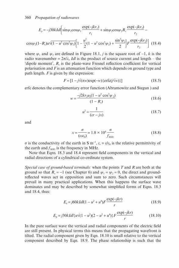
Eρ = −j30kIdlsinψ1cosψ1
exp(−jkr1)
r1
+ sinψ2cosψ2Rν
exp(−jkr2)
r2
−
cosψ2(1−Rν)u√(1 − u2 cos2ψ2)�1 − u2
2(1 − u2 cos2ψ2) +
sin2ψ2
2 �F exp(−jkr2)
r2� (18.4)
where ψ1 and ψ2 are defined in Figure 18.1, j is the square root of −1, k is theradio wavenumber = 2π/λ, Idl is the product of source current and length – the‘dipole moment’, Rν is the plane-wave Fresnel reflection coefficient for verticalpolarisation and F is an attenuation function which depends on ground type andpath length. F is given by the expression:
F = [1 − j√(πw)exp(−w){erfc(j√w)}] (18.5)
erfc denotes the complementary error function (Abramowitz and Stegun ) and
w = −j2kr2u2(1 − u2 cos2ψ 2)
(1 − Rν)(18.6)
u2 = 1
(εr − jx)(18.7)
and
x = σ
(ωε0) = 1.8 × 10⁴
σ
fMHz
(18.8)
σ is the conductivity of the earth in S m−1, εr = ε/ε0 is the relative permittivity ofthe earth and fMHz is the frequency in MHz.
Note that Eqns. 18.3 and 18.4 represent field components in the vertical andradial directions of a cylindrical co-ordinate system.
Special case of ground-based terminals: when the points T and R are both at theground so that Rν = −1 (see Chapter 6) and ψ1 = ψ2 = 0, the direct and ground-reflected waves act in opposition and sum to zero. Such circumstances willprevail in many practical applications. When this happens the surface wavedominates and may be described by somewhat simplified forms of Eqns. 18.3and 18.4, thus:
Ez = j60kIdl(1 − u2 + u4)F exp(−jkr)
r(18.9)
Ep = j30kIdl{u√(1 − u2)(2 − u2 + u4)}Fexp(−jkr)
r(18.10)
In the pure surface wave the vertical and radial components of the electric fieldare still present. In physical terms this means that the propagating wavefront istilted. The radial component given by Eqn. 18.10 is small relative to the verticalcomponent described by Eqn. 18.9. The phase relationship is such that the
360 Propagation of radiowaves
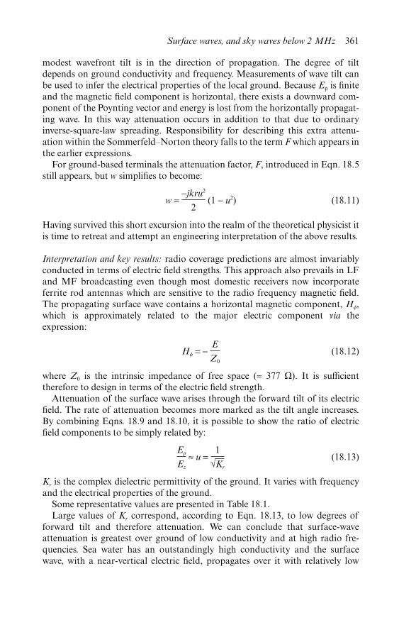
modest wavefront tilt is in the direction of propagation. The degree of tiltdepends on ground conductivity and frequency. Measurements of wave tilt canbe used to infer the electrical properties of the local ground. Because Ep is finiteand the magnetic field component is horizontal, there exists a downward com-ponent of the Poynting vector and energy is lost from the horizontally propagat-ing wave. In this way attenuation occurs in addition to that due to ordinaryinverse-square-law spreading. Responsibility for describing this extra attenu-ation within the Sommerfeld–Norton theory falls to the term F which appears inthe earlier expressions.
For ground-based terminals the attenuation factor, F, introduced in Eqn. 18.5still appears, but w simplifies to become:
w = −jkru2
2(1 − u2) (18.11)
Having survived this short excursion into the realm of the theoretical physicist itis time to retreat and attempt an engineering interpretation of the above results.
Interpretation and key results: radio coverage predictions are almost invariablyconducted in terms of electric field strengths. This approach also prevails in LFand MF broadcasting even though most domestic receivers now incorporateferrite rod antennas which are sensitive to the radio frequency magnetic field.The propagating surface wave contains a horizontal magnetic component, H,which is approximately related to the major electric component via theexpression:
H = −E
Z0
(18.12)
where Z0 is the intrinsic impedance of free space (≈ 377 Ω). It is sufficienttherefore to design in terms of the electric field strength.
Attenuation of the surface wave arises through the forward tilt of its electricfield. The rate of attenuation becomes more marked as the tilt angle increases.By combining Eqns. 18.9 and 18.10, it is possible to show the ratio of electricfield components to be simply related by:
Eρ
Ez
≈ u = 1
√Kr
(18.13)
Kr is the complex dielectric permittivity of the ground. It varies with frequencyand the electrical properties of the ground.
Some representative values are presented in Table 18.1.Large values of Kr correspond, according to Eqn. 18.13, to low degrees of
forward tilt and therefore attenuation. We can conclude that surface-waveattenuation is greatest over ground of low conductivity and at high radio fre-quencies. Sea water has an outstandingly high conductivity and the surfacewave, with a near-vertical electric field, propagates over it with relatively low
Surface waves, and sky waves below 2 MHz 361
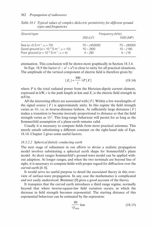
attenuation. This conclusion will be shown more graphically in Section 18.3.4.In Eqn. 18.9 the factor (1 − u2 + u4) is close to unity for all practical situations.
The amplitude of the vertical component of electric field is therefore given by:
| Ez | = 300
r √P | F | (18.14)
where P is the total radiated power from the Hertzian-dipole current element,expressed in kW, r is the path length in km and Ez is the electric field strength inmV/m.
All the interesting effects are associated with | F |. Within a few wavelengths ofthe signal source | F | is approximately unity. In this regime the field strengthvaries as 1/r, i.e. in inverse-distance fashion. At sufficiently large distances | F |makes a transition to become inversely proportional to distance so that the fieldstrength varies as 1/r2. This long-range behaviour will persist for as long as theSommerfeld assumption of a plane earth remains valid.
Usually it is necessary to compute fields from more practical antennas. Thismerely entails substituting a different constant on the right-hand side of Eqn.18.14. Chapter 2 gives some useful factors.
18.3.2.2 Spherical finitely conducting earth
The next stage of refinement in our efforts to devise a realistic propagationmodel involves substituting a spherical earth shape for Sommerfeld’s planemodel. At short ranges Sommerfeld’s ground-wave model can be applied with-out adaption. At longer ranges, and when the two terminals are beyond line ofsight, it is necessary to compute fields with proper regard for diffraction over thecurved earth [4–8].
It would serve no useful purpose to detail the associated theory in this over-view of surface-wave propagation. In any case the mathematics is complicatedand not easily understood. Bremmer [9] gives a good account of the theory.
It transpires that the curved earth introduces a third range regime, normallybeyond that where inverse-square-law field variation occurs, in which thedecrease in field strength becomes exponential. The starting distance of thisexponential behaviour can be estimated by the expression:
80
√fMHz
km (18.15)
Table 18.1 Typical values of complex dielectric permittivity for different groundtypes and frequencies
Ground type Frequency (kHz)200 (LF) 1000 (MF)
Sea (σ =5 S m−1, εr = 70) 70 − j450000 70 − j90000Good ground (σ = 10−2 S m−1, εr = 10) 10 − j900 10 − j180Poor ground (σ = 10−3 S m−1, εr = 4) 4 − j90 4 − j18
362 Propagation of radiowaves
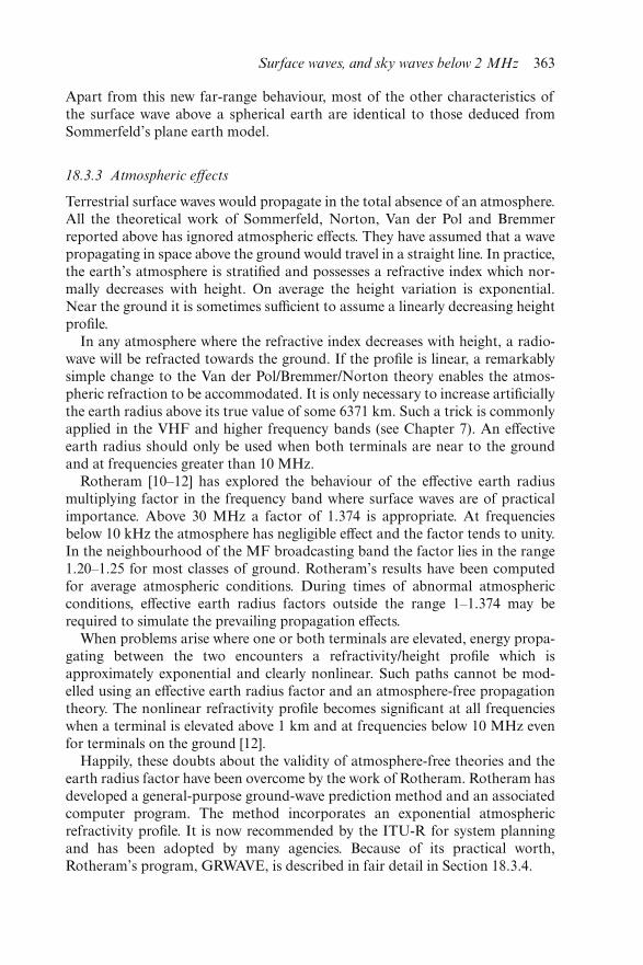
Apart from this new far-range behaviour, most of the other characteristics ofthe surface wave above a spherical earth are identical to those deduced fromSommerfeld’s plane earth model.
18.3.3 Atmospheric effects
Terrestrial surface waves would propagate in the total absence of an atmosphere.All the theoretical work of Sommerfeld, Norton, Van der Pol and Bremmerreported above has ignored atmospheric effects. They have assumed that a wavepropagating in space above the ground would travel in a straight line. In practice,the earth’s atmosphere is stratified and possesses a refractive index which nor-mally decreases with height. On average the height variation is exponential.Near the ground it is sometimes sufficient to assume a linearly decreasing heightprofile.
In any atmosphere where the refractive index decreases with height, a radio-wave will be refracted towards the ground. If the profile is linear, a remarkablysimple change to the Van der Pol/Bremmer/Norton theory enables the atmos-pheric refraction to be accommodated. It is only necessary to increase artificiallythe earth radius above its true value of some 6371 km. Such a trick is commonlyapplied in the VHF and higher frequency bands (see Chapter 7). An effectiveearth radius should only be used when both terminals are near to the groundand at frequencies greater than 10 MHz.
Rotheram [10–12] has explored the behaviour of the effective earth radiusmultiplying factor in the frequency band where surface waves are of practicalimportance. Above 30 MHz a factor of 1.374 is appropriate. At frequenciesbelow 10 kHz the atmosphere has negligible effect and the factor tends to unity.In the neighbourhood of the MF broadcasting band the factor lies in the range1.20–1.25 for most classes of ground. Rotheram’s results have been computedfor average atmospheric conditions. During times of abnormal atmosphericconditions, effective earth radius factors outside the range 1–1.374 may berequired to simulate the prevailing propagation effects.
When problems arise where one or both terminals are elevated, energy propa-gating between the two encounters a refractivity/height profile which isapproximately exponential and clearly nonlinear. Such paths cannot be mod-elled using an effective earth radius factor and an atmosphere-free propagationtheory. The nonlinear refractivity profile becomes significant at all frequencieswhen a terminal is elevated above 1 km and at frequencies below 10 MHz evenfor terminals on the ground [12].
Happily, these doubts about the validity of atmosphere-free theories and theearth radius factor have been overcome by the work of Rotheram. Rotheram hasdeveloped a general-purpose ground-wave prediction method and an associatedcomputer program. The method incorporates an exponential atmosphericrefractivity profile. It is now recommended by the ITU-R for system planningand has been adopted by many agencies. Because of its practical worth,Rotheram’s program, GRWAVE, is described in fair detail in Section 18.3.4.
Surface waves, and sky waves below 2 MHz 363
18.3.4 ITU-R recommended prediction method
Rotheram describes three methods of predicting space-wave and surface-wavefields over a smooth homogeneous earth surrounded by a uniform atmospherewhich exhibits an exponential refractivity/height profile. The methods cater forelevated terminals and a very wide frequency band. No single method is effec-tive for all path geometries but, using appropriate numerical techniques, it ispossible to establish whether or not one method is working and, if it is not,switch to a better approach. The methods and their approximate regions ofvalidity are:
(i) Residue series (mode summation): used at the farthest distances, for ele-vated terminals this is beyond the radio horizon. For terminals near theearth’s surface it is for distances greater than approximately 10 λ1/3 kmwhere λ is the radio wavelength in metres.
(ii) Extended Sommerfeld flat-earth theory: an extended Sommerfeld theorycan be applied at short ranges and small heights. These restrictions turnout to be ranges less than approximately 10 λ1/3 km and heights below35 λ2/3 m.
(iii) Geometrical optics (ray theory): this final method is applied within theradio horizon when the terminal heights are above that which can behandled by the Sommerfeld approach. It involves calculating the phaseand amplitude of the direct and ground-reflected paths with due regard forthe atmospheric refraction.
Fortunately, the three methods are able to deal with all reasonable geometries sothat inelegant interpolation between two inappropriate results is unnecessary.Under circumstances where two methods are simultaneously valid the results arefound to be in good agreement.
Rotheram has written a Fortran computer program to compute ground-wavefields using these theories. This program, GRWAVE, has been used by the ITU-R to produce a series of curves which show how vertically polarised electricalfield strength varies as a function of range, ground type and frequency (10 kHzto 30 MHz). In doing this the ITU-R has elected to adopt a global averagerefractivity profile given by:
n = 1 + (ns − 1)exp(−h/hs) (18.16)
where ns = surface refractivity = 1.000315 and hs = refractivity profile scale height= 7.35 km. These curves are to be found in Recommendation ITU-R P.368 [13].
Although the ITU-R curves are comprehensive, it is sometimes useful to useGRWAVE program itself.
Figure 18.2 shows some example ITU-R ground-wave curves for sea, land(σ = 0.03 S m−1) and very dry ground (σ = 0.000 1 S m−1). The latter two representsome extreme ground conditions. Sea is best regarded as being in a class of itsown. For these curves both terminals are on the ground so that, in their compu-tation, the geometrical optics parts of GRWAVE will not have been invoked.A close inspection of Figure 18.2 will reveal the inverse-distance,
364 Propagation of radiowaves
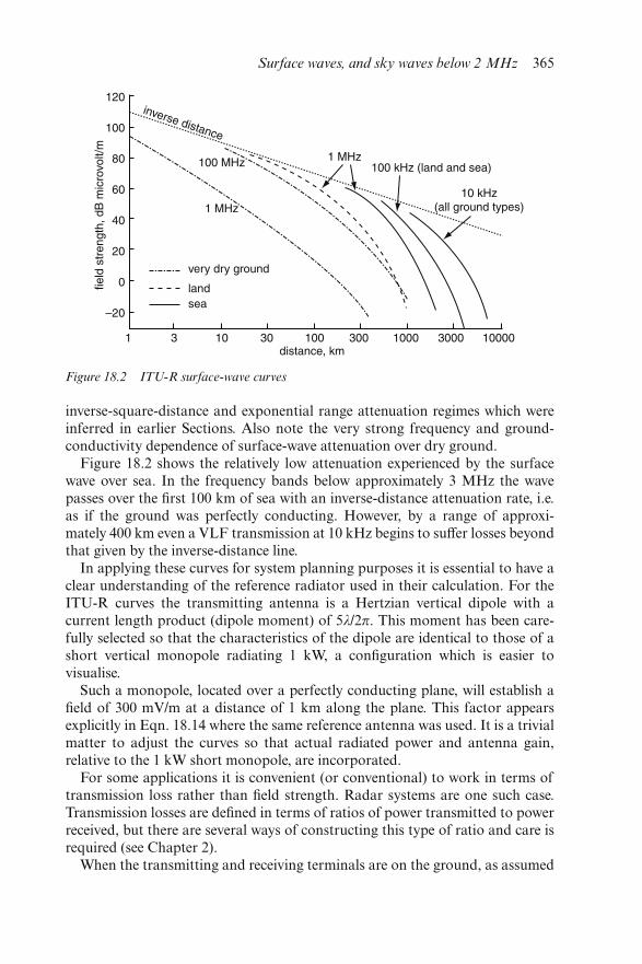
inverse-square-distance and exponential range attenuation regimes which wereinferred in earlier Sections. Also note the very strong frequency and ground-conductivity dependence of surface-wave attenuation over dry ground.
Figure 18.2 shows the relatively low attenuation experienced by the surfacewave over sea. In the frequency bands below approximately 3 MHz the wavepasses over the first 100 km of sea with an inverse-distance attenuation rate, i.e.as if the ground was perfectly conducting. However, by a range of approxi-mately 400 km even a VLF transmission at 10 kHz begins to suffer losses beyondthat given by the inverse-distance line.
In applying these curves for system planning purposes it is essential to have aclear understanding of the reference radiator used in their calculation. For theITU-R curves the transmitting antenna is a Hertzian vertical dipole with acurrent length product (dipole moment) of 5λ/2π. This moment has been care-fully selected so that the characteristics of the dipole are identical to those of ashort vertical monopole radiating 1 kW, a configuration which is easier tovisualise.
Such a monopole, located over a perfectly conducting plane, will establish afield of 300 mV/m at a distance of 1 km along the plane. This factor appearsexplicitly in Eqn. 18.14 where the same reference antenna was used. It is a trivialmatter to adjust the curves so that actual radiated power and antenna gain,relative to the 1 kW short monopole, are incorporated.
For some applications it is convenient (or conventional) to work in terms oftransmission loss rather than field strength. Radar systems are one such case.Transmission losses are defined in terms of ratios of power transmitted to powerreceived, but there are several ways of constructing this type of ratio and care isrequired (see Chapter 2).
When the transmitting and receiving terminals are on the ground, as assumed
Figure 18.2 ITU-R surface-wave curves
Surface waves, and sky waves below 2 MHz 365
in Figure 18.2, it is easy to relate ITU-R field strength curves to basic transmis-sion loss:
Lb = 142.0 + 20 log10 fMHz − E (18.17)
where E is the field strength, in dB (μV m−1) for the ITU-R reference radiator.The frequency term in the above equation arises because the collecting aper-
ture of a receiving antenna, and therefore the power available, depends on radiofrequency.
ITU-R Recommendation P.341 [14] and Chapter 2 discuss the use of Lb insystem design calculations. This will not be reiterated here. It is, however,important to address one key point and this relates to the antenna gain defini-tion which must be used when Lb is involved. In the system calculation, actualantenna gains must be introduced as relative to an isotropic antenna at the samelocation. This is not the convention commonly used by antenna manufacturersin their sales literature. They tend to use dB relative to a truly isotropic antennain free space.
This apparently trivial matter of antenna gain in ground and surface-wavepath-loss calculations can lead to great confusion and, worse, an incorrect sys-tem design. The problem is compounded by the existence of several different(but internally consistent) sets of definitions and papers in the open literaturewhich present vague or incorrect accounts of antenna gain.
18.3.5 Ground conductivity maps
In practice, when the propagation engineer has been asked to compute the via-bility of a link or the coverage of a broadcasting station, one of the mostdifficult stages is to acquire a proper description of the ground conductivityalong the path or in the area of interest. A useful source of data lies in ITU-RRecommendation P.832 [15]. Here, geographic maps are presented on whichareas of differing electrical properties are delineated. The maps are a con-glomerate of information collected over many years, and the degree of detailvaries from region to region.
Once the ITU-R maps have been consulted, it is often worth seeking sup-plementary local information about the ground types present. Broadcastingauthorities sometimes have details of ground conductivity in their areas whichmay not have found its way into Recommendation P.832.
When the ITU-R and local information sources both prove to be inadequate,it is sometimes instructive to consult geological maps of the district and attemptan association of mineral type with electrical properties.
18.3.6 Smooth earth of mixed conductivity
So far we have discussed increasingly elaborate models of surface-wavepropagation and the ways in which they might be applied. However, all of themodels only treat the case of a homogeneous smooth earth. In practice, it is
366 Propagation of radiowaves
often necessary to solve planning problems which involve changes in groundtype along the propagation path.
Suppose we have a situation where a surface-wave link must be establishedbetween two terminals which are located on ground of different electrical pro-perties. At some point along the smooth propagation path a transition occursbetween the two ground types. The upper half of Figure 18.3 shows the situationin schematic form. How do we compute the electric field strength at R due to thetransmission from T?
Eckersley suggested that this might be done by using sections of the surface-wave attenuation curves appropriate to the radio frequency and different groundtypes. Figure 18.3 shows the idea in graphical form. The Eckersley constructioncan be made using the curves for homogeneous ground such as those publishedby the ITU-R. Intuitively, this method appears correct. However, it producesresults in poor agreement with experiment and, furthermore, violates the need tohave reciprocity on the path. Reciprocity demands that, if the transmitter andreceiver were transposed, so that the wave encountered the two types of groundin reverse order, then the field strength at the receiver would be unchanged.
Millington, in a classic paper on ground-wave propagation, presented asimple but effective method of solving the problem depicted in Figure 18.3. Hiswork was done at a time when reliable measurements of field strength changes inthe neighbourhood of a conductivity transition were scarce. Others were devel-oping analytic solutions to the problem but their results were complicated andunsuitable for practical application. Millington’s approach was a blend ofknown theory and physical intuition. The argument proceeded along thefollowing lines.
Suppose T in Figure 18.3 is well removed from the conductivity transition atX. In this case the surface wave which is launched in the direction of R will havea rate of attenuation with horizontal distance and a variation with height aboveground which is characteristic of ground type 1. The field can be computedusing a model for the homogeneous earth with little loss of accuracy. Similarly,if R is well removed from X then the surface-wave field strength will vary withhorizontal distance and height in a way which is largely dictated by the groundtype 2. In effect, it might appear as if the signal had travelled from T to R overhomogeneous ground of type 2. The only residual evidence of its passage overthe type 1 ground will be a shift in the absolute signal level. Homogeneous earthpropagation models cannot be applied directly to compute the absolute fieldstrength on the receiver side of X.
Consider now what might be happening close to the conductivity transitionpoint X. Millington argued that some sort of distortion or disturbance of thesurface wave must occur. On approaching the transition from T the field willprobably be affected even before X itself is encountered. However, this must bemodest in comparison with the trauma undergone by the field on the receiverside of the transition.
Millington then elaborated the discussion and sought to establish a predictionmethod which would give a consistent change in the height profile of the field
Surface waves, and sky waves below 2 MHz 367
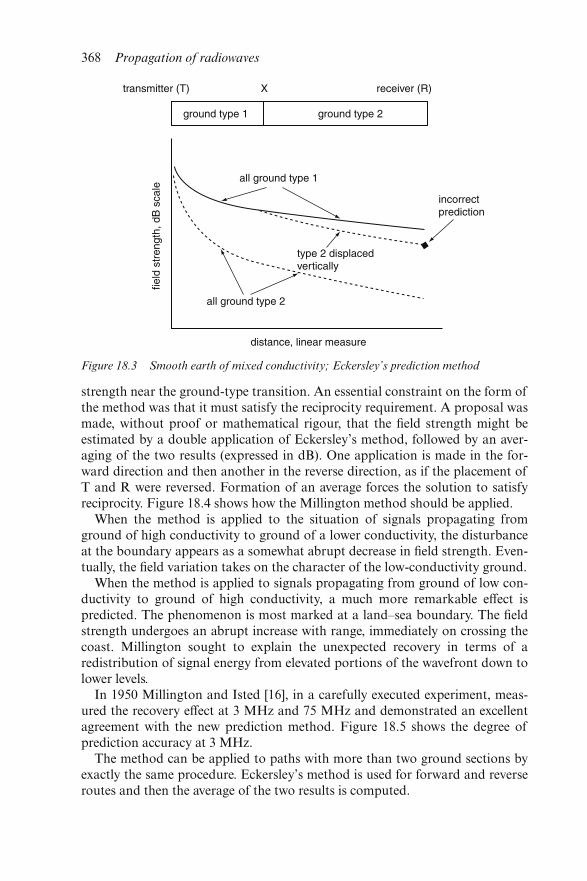
strength near the ground-type transition. An essential constraint on the form ofthe method was that it must satisfy the reciprocity requirement. A proposal wasmade, without proof or mathematical rigour, that the field strength might beestimated by a double application of Eckersley’s method, followed by an aver-aging of the two results (expressed in dB). One application is made in the for-ward direction and then another in the reverse direction, as if the placement ofT and R were reversed. Formation of an average forces the solution to satisfyreciprocity. Figure 18.4 shows how the Millington method should be applied.
When the method is applied to the situation of signals propagating fromground of high conductivity to ground of a lower conductivity, the disturbanceat the boundary appears as a somewhat abrupt decrease in field strength. Even-tually, the field variation takes on the character of the low-conductivity ground.
When the method is applied to signals propagating from ground of low con-ductivity to ground of high conductivity, a much more remarkable effect ispredicted. The phenomenon is most marked at a land–sea boundary. The fieldstrength undergoes an abrupt increase with range, immediately on crossing thecoast. Millington sought to explain the unexpected recovery in terms of aredistribution of signal energy from elevated portions of the wavefront down tolower levels.
In 1950 Millington and Isted [16], in a carefully executed experiment, meas-ured the recovery effect at 3 MHz and 75 MHz and demonstrated an excellentagreement with the new prediction method. Figure 18.5 shows the degree ofprediction accuracy at 3 MHz.
The method can be applied to paths with more than two ground sections byexactly the same procedure. Eckersley’s method is used for forward and reverseroutes and then the average of the two results is computed.
Figure 18.3 Smooth earth of mixed conductivity; Eckersley’s prediction method
368 Propagation of radiowaves
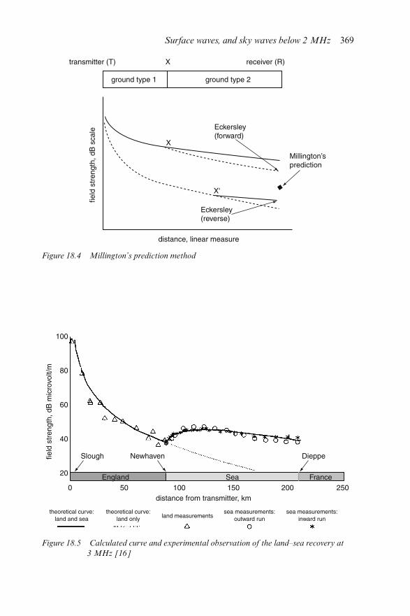
Figure 18.4 Millington’s prediction method
Figure 18.5 Calculated curve and experimental observation of the land–sea recovery at
3 MHz [16]
Surface waves, and sky waves below 2 MHz 369
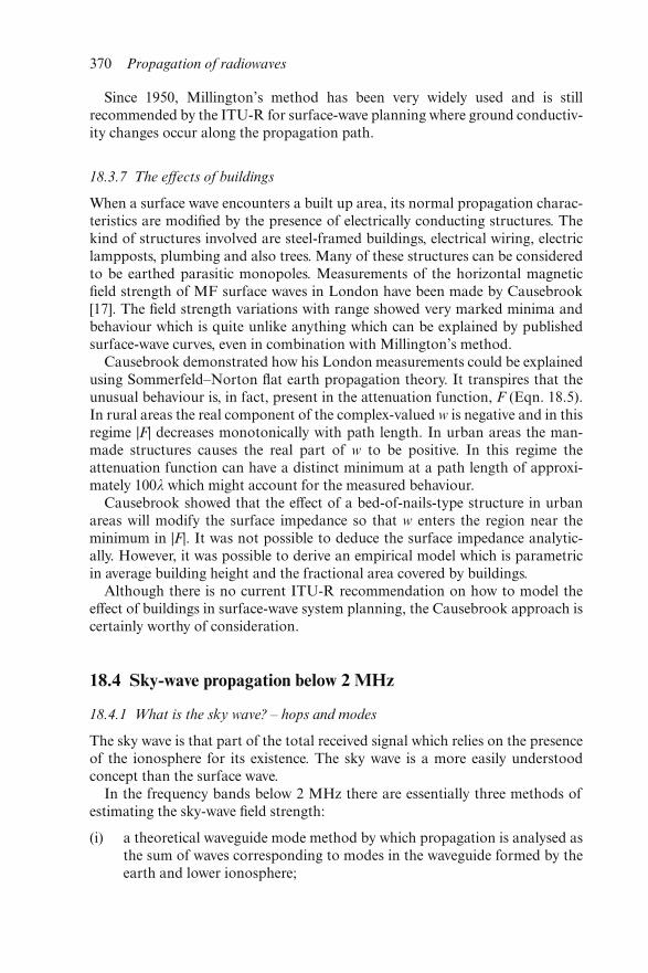
Since 1950, Millington’s method has been very widely used and is stillrecommended by the ITU-R for surface-wave planning where ground conductiv-ity changes occur along the propagation path.
18.3.7 The effects of buildings
When a surface wave encounters a built up area, its normal propagation charac-teristics are modified by the presence of electrically conducting structures. Thekind of structures involved are steel-framed buildings, electrical wiring, electriclampposts, plumbing and also trees. Many of these structures can be consideredto be earthed parasitic monopoles. Measurements of the horizontal magneticfield strength of MF surface waves in London have been made by Causebrook[17]. The field strength variations with range showed very marked minima andbehaviour which is quite unlike anything which can be explained by publishedsurface-wave curves, even in combination with Millington’s method.
Causebrook demonstrated how his London measurements could be explainedusing Sommerfeld–Norton flat earth propagation theory. It transpires that theunusual behaviour is, in fact, present in the attenuation function, F (Eqn. 18.5).In rural areas the real component of the complex-valued w is negative and in thisregime |F| decreases monotonically with path length. In urban areas the man-made structures causes the real part of w to be positive. In this regime theattenuation function can have a distinct minimum at a path length of approxi-mately 100λ which might account for the measured behaviour.
Causebrook showed that the effect of a bed-of-nails-type structure in urbanareas will modify the surface impedance so that w enters the region near theminimum in |F|. It was not possible to deduce the surface impedance analytic-ally. However, it was possible to derive an empirical model which is parametricin average building height and the fractional area covered by buildings.
Although there is no current ITU-R recommendation on how to model theeffect of buildings in surface-wave system planning, the Causebrook approach iscertainly worthy of consideration.
18.4 Sky-wave propagation below 2 MHz
18.4.1 What is the sky wave? – hops and modes
The sky wave is that part of the total received signal which relies on the presenceof the ionosphere for its existence. The sky wave is a more easily understoodconcept than the surface wave.
In the frequency bands below 2 MHz there are essentially three methods ofestimating the sky-wave field strength:
(i) a theoretical waveguide mode method by which propagation is analysed asthe sum of waves corresponding to modes in the waveguide formed by theearth and lower ionosphere;
370 Propagation of radiowaves
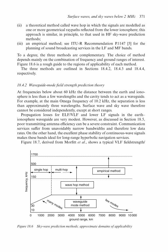
(ii) a theoretical method called wave hop in which the signals are modelled asone or more geometrical raypaths reflected from the lower ionosphere; thisapproach is similar, in principle, to that used in HF sky-wave predictionmethods;
(iii) an empirical method; see ITU-R Recommendation P.1147 [5] for theplanning of sound broadcasting services in the LF and MF bands.
To a degree, the three methods are complementary. The choice of methoddepends mainly on the combination of frequency and ground ranges of interest.Figure 18.6 is a rough guide to the regions of applicability of each method.
The three methods are outlined in Sections 18.4.2, 18.4.3 and 18.4.4,respectively.
18.4.2 Waveguide-mode field strength prediction theory
At frequencies below about 60 kHz the distance between the earth and iono-sphere is less than a few wavelengths and the cavity tends to act as a waveguide.For example, at the main Omega frequency of 10.2 kHz, the separation is lessthan approximately three wavelengths. Surface wave and sky wave thereforecannot be considered independently, except at short ranges.
Propagation losses for ELF/VLF and lower LF signals in the earth–ionosphere waveguide are very modest. However, as discussed in Section 18.5,poor transmitting antenna efficiency can be a severe constraint. Communicationservices suffer from unavoidably narrow bandwidths and therefore low datarates. On the other hand, the excellent phase stability of continuous-wave signalsmakes these bands ideal for long-range hyperbolic navigation services.
Figure 18.7, derived from Morfitt et al., shows a typical VLF fieldstrength/
Figure 18.6 Sky-wave prediction methods; approximate domains of applicability
Surface waves, and sky waves below 2 MHz 371
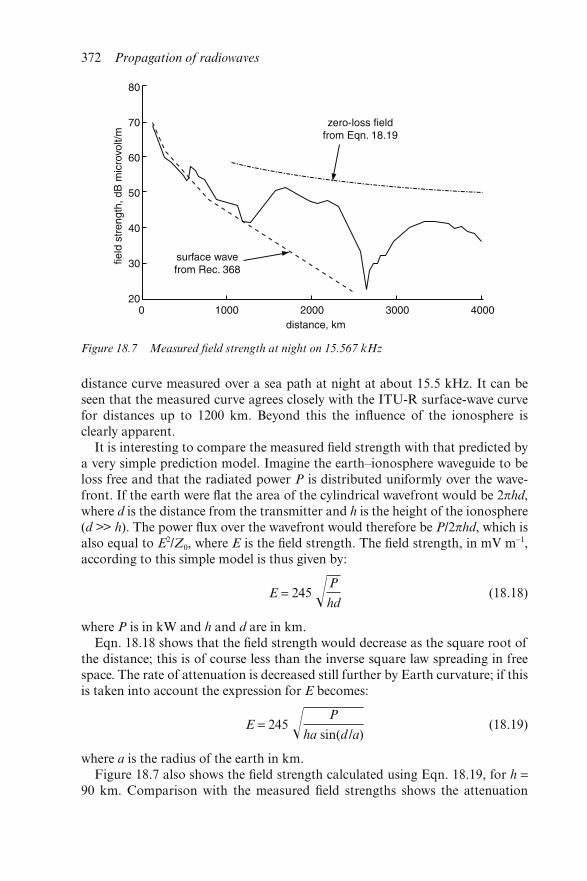
distance curve measured over a sea path at night at about 15.5 kHz. It can beseen that the measured curve agrees closely with the ITU-R surface-wave curvefor distances up to 1200 km. Beyond this the influence of the ionosphere isclearly apparent.
It is interesting to compare the measured field strength with that predicted bya very simple prediction model. Imagine the earth–ionosphere waveguide to beloss free and that the radiated power P is distributed uniformly over the wave-front. If the earth were flat the area of the cylindrical wavefront would be 2πhd,where d is the distance from the transmitter and h is the height of the ionosphere(d >> h). The power flux over the wavefront would therefore be P/2πhd, which isalso equal to E2/Z0, where E is the field strength. The field strength, in mV m−1,according to this simple model is thus given by:
E = 245 �P
hd(18.18)
where P is in kW and h and d are in km.Eqn. 18.18 shows that the field strength would decrease as the square root of
the distance; this is of course less than the inverse square law spreading in freespace. The rate of attenuation is decreased still further by Earth curvature; if thisis taken into account the expression for E becomes:
E = 245 � P
ha sin(d /a)(18.19)
where a is the radius of the earth in km.Figure 18.7 also shows the field strength calculated using Eqn. 18.19, for h =
90 km. Comparison with the measured field strengths shows the attenuation
Figure 18.7 Measured field strength at night on 15.567 kHz
372 Propagation of radiowaves
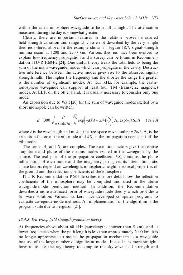
within the earth–ionosphere waveguide to be small at night. The attenuationmeasured during the day is somewhat greater.
Clearly, there are important features in the relation between measuredfield-strength variation and range which are not described by the very simpletheories offered above. In the example shown in Figure 18.7, signal-strengthminima occur at 1200 and 2700 km. Various theories have been evolved toexplain low-frequency propagation and a survey can be found in Recommen-dation ITU-R P.684-2 [24]. One useful theory treats the total field as being thesum of the main waveguide modes which can propagate in the cavity. Destruc-tive interference between the active modes gives rise to the observed signal-strength nulls. The higher the frequency and the shorter the range the greateris the number of significant modes. At 15.5 kHz, for example, the earth–ionosphere waveguide can support at least four TM (transverse magnetic)modes. At ELF, on the other hand, it is usually necessary to consider only onemode.
An expression due to Wait [20] for the sum of waveguide modes excited by ashort monopole can be written:
E = 300 � P
a sin(d /a) √λ
h exp�−j(kd + π/4)��
n
Λn exp(−jkSnd) (18.20)
where λ is the wavelength, in km, k is the free-space wavenumber = 2π/λ, Λn is theexcitation factor of the nth mode and kSn is the propagation coefficient of thenth mode.
The terms Λn and Sn are complex. The excitation factors give the relativeamplitude and phase of the various modes excited in the waveguide by thesource. The real part of the propagation coefficient kSn contains the phaseinformation of each mode and the imaginary part gives its attenuation rate.These factors depend on wavelength, ionospheric height, electrical properties ofthe ground and the reflection coefficients of the ionosphere.
ITU-R Recommendation P.684 describes in more detail how the reflectioncoefficients of the ionosphere may be computed and used in the abovewaveguide-mode prediction method. In addition, the Recommendationdescribes a more advanced form of waveguide-mode theory which provides afull-wave solution. Various workers have developed computer programs toevaluate waveguide-mode methods. An implementation of the algorithm is theprogram suite due to Ferguson [21].
18.4.3 Wave-hop field strength prediction theory
At frequencies above about 60 kHz (wavelengths shorter than 5 km), and atlower frequencies when the path length is less than approximately 2000 km, it isno longer appropriate to model the propagation mechanism as a waveguidebecause of the large number of significant modes. Instead it is more straight-forward to use the ray theory to compute the sky-wave field strength and
Surface waves, and sky waves below 2 MHz 373
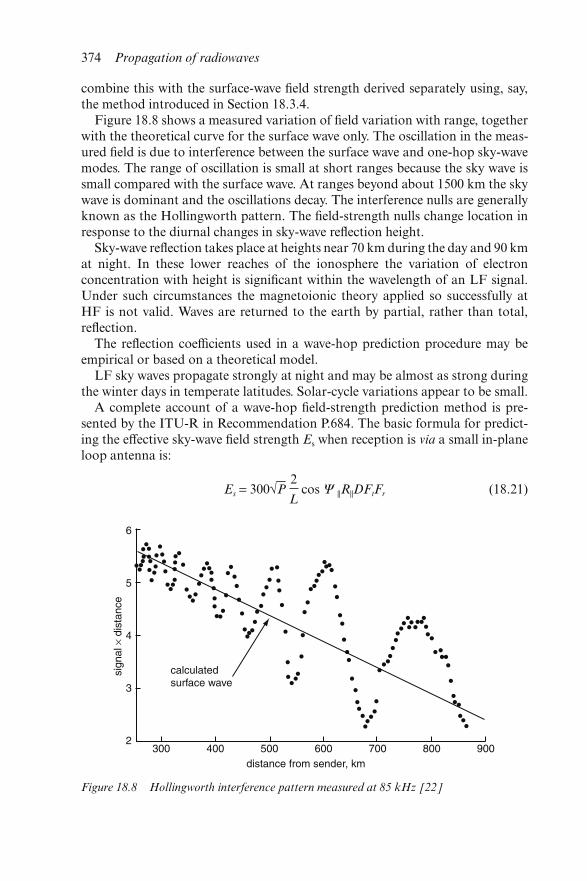
combine this with the surface-wave field strength derived separately using, say,the method introduced in Section 18.3.4.
Figure 18.8 shows a measured variation of field variation with range, togetherwith the theoretical curve for the surface wave only. The oscillation in the meas-ured field is due to interference between the surface wave and one-hop sky-wavemodes. The range of oscillation is small at short ranges because the sky wave issmall compared with the surface wave. At ranges beyond about 1500 km the skywave is dominant and the oscillations decay. The interference nulls are generallyknown as the Hollingworth pattern. The field-strength nulls change location inresponse to the diurnal changes in sky-wave reflection height.
Sky-wave reflection takes place at heights near 70 km during the day and 90 kmat night. In these lower reaches of the ionosphere the variation of electronconcentration with height is significant within the wavelength of an LF signal.Under such circumstances the magnetoionic theory applied so successfully atHF is not valid. Waves are returned to the earth by partial, rather than total,reflection.
The reflection coefficients used in a wave-hop prediction procedure may beempirical or based on a theoretical model.
LF sky waves propagate strongly at night and may be almost as strong duringthe winter days in temperate latitudes. Solar-cycle variations appear to be small.
A complete account of a wave-hop field-strength prediction method is pre-sented by the ITU-R in Recommendation P.684. The basic formula for predict-ing the effective sky-wave field strength Es when reception is via a small in-planeloop antenna is:
Es = 300√P 2
L cos Ψ ||R||DFtFr (18.21)
Figure 18.8 Hollingworth interference pattern measured at 85 kHz [22]
374 Propagation of radiowaves
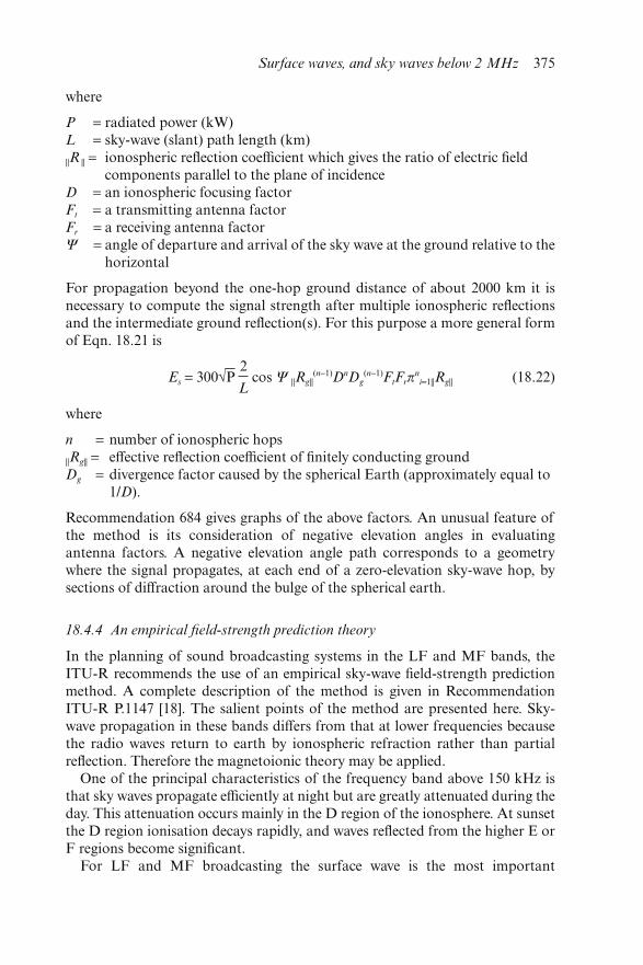
where
P = radiated power (kW)L = sky-wave (slant) path length (km)||R || = ionospheric reflection coefficient which gives the ratio of electric field
components parallel to the plane of incidenceD = an ionospheric focusing factorFt = a transmitting antenna factorFr = a receiving antenna factorΨ = angle of departure and arrival of the sky wave at the ground relative to the
horizontal
For propagation beyond the one-hop ground distance of about 2000 km it isnecessary to compute the signal strength after multiple ionospheric reflectionsand the intermediate ground reflection(s). For this purpose a more general formof Eqn. 18.21 is
Es = 300√P 2
L cos Ψ ||Rg||
(n−1)DnDg(n−1)FtFrπ
ni=1||Rg|| (18.22)
where
n = number of ionospheric hops||Rg|| = effective reflection coefficient of finitely conducting groundDg = divergence factor caused by the spherical Earth (approximately equal to
1/D).
Recommendation 684 gives graphs of the above factors. An unusual feature ofthe method is its consideration of negative elevation angles in evaluatingantenna factors. A negative elevation angle path corresponds to a geometrywhere the signal propagates, at each end of a zero-elevation sky-wave hop, bysections of diffraction around the bulge of the spherical earth.
18.4.4 An empirical field-strength prediction theory
In the planning of sound broadcasting systems in the LF and MF bands, theITU-R recommends the use of an empirical sky-wave field-strength predictionmethod. A complete description of the method is given in RecommendationITU-R P.1147 [18]. The salient points of the method are presented here. Sky-wave propagation in these bands differs from that at lower frequencies becausethe radio waves return to earth by ionospheric refraction rather than partialreflection. Therefore the magnetoionic theory may be applied.
One of the principal characteristics of the frequency band above 150 kHz isthat sky waves propagate efficiently at night but are greatly attenuated during theday. This attenuation occurs mainly in the D region of the ionosphere. At sunsetthe D region ionisation decays rapidly, and waves reflected from the higher E orF regions become significant.
For LF and MF broadcasting the surface wave is the most important
Surface waves, and sky waves below 2 MHz 375
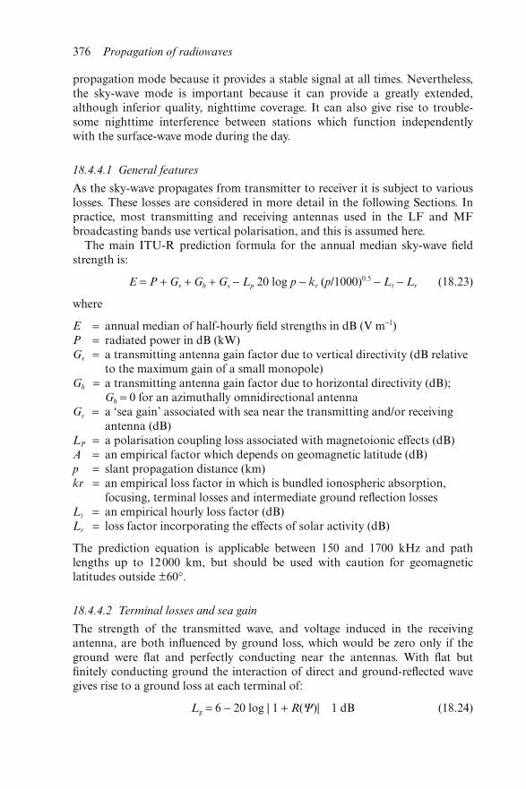
propagation mode because it provides a stable signal at all times. Nevertheless,the sky-wave mode is important because it can provide a greatly extended,although inferior quality, nighttime coverage. It can also give rise to trouble-some nighttime interference between stations which function independentlywith the surface-wave mode during the day.
18.4.4.1 General features
As the sky-wave propagates from transmitter to receiver it is subject to variouslosses. These losses are considered in more detail in the following Sections. Inpractice, most transmitting and receiving antennas used in the LF and MFbroadcasting bands use vertical polarisation, and this is assumed here.
The main ITU-R prediction formula for the annual median sky-wave fieldstrength is:
E = P + Gv + Gh + Gs − Lp 20 log p − kr (p/1000)0.5 − Lt − Lr (18.23)
where
E = annual median of half-hourly field strengths in dB (V m−1)P = radiated power in dB (kW)Gv = a transmitting antenna gain factor due to vertical directivity (dB relative
to the maximum gain of a small monopole)Gh = a transmitting antenna gain factor due to horizontal directivity (dB);
Gh = 0 for an azimuthally omnidirectional antennaGs = a ‘sea gain’ associated with sea near the transmitting and/or receiving
antenna (dB)LP = a polarisation coupling loss associated with magnetoionic effects (dB)A = an empirical factor which depends on geomagnetic latitude (dB)p = slant propagation distance (km)kr = an empirical loss factor in which is bundled ionospheric absorption,
focusing, terminal losses and intermediate ground reflection lossesLt = an empirical hourly loss factor (dB)Lr = loss factor incorporating the effects of solar activity (dB)
The prediction equation is applicable between 150 and 1700 kHz and pathlengths up to 12000 km, but should be used with caution for geomagneticlatitudes outside ±60°.
18.4.4.2 Terminal losses and sea gain
The strength of the transmitted wave, and voltage induced in the receivingantenna, are both influenced by ground loss, which would be zero only if theground were flat and perfectly conducting near the antennas. With flat butfinitely conducting ground the interaction of direct and ground-reflected wavegives rise to a ground loss at each terminal of:
Lg = 6 − 20 log | 1 + R(Ψ)| 1 dB (18.24)
376 Propagation of radiowaves
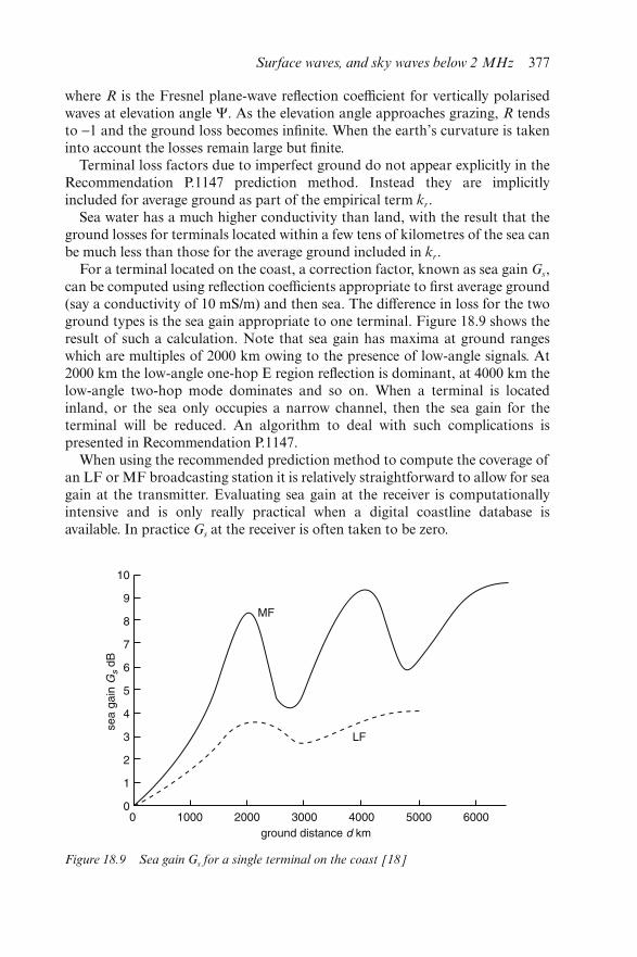
where R is the Fresnel plane-wave reflection coefficient for vertically polarisedwaves at elevation angle Ψ. As the elevation angle approaches grazing, R tendsto −1 and the ground loss becomes infinite. When the earth’s curvature is takeninto account the losses remain large but finite.
Terminal loss factors due to imperfect ground do not appear explicitly in theRecommendation P.1147 prediction method. Instead they are implicitlyincluded for average ground as part of the empirical term kr.
Sea water has a much higher conductivity than land, with the result that theground losses for terminals located within a few tens of kilometres of the sea canbe much less than those for the average ground included in kr.
For a terminal located on the coast, a correction factor, known as sea gain Gs,can be computed using reflection coefficients appropriate to first average ground(say a conductivity of 10 mS/m) and then sea. The difference in loss for the twoground types is the sea gain appropriate to one terminal. Figure 18.9 shows theresult of such a calculation. Note that sea gain has maxima at ground rangeswhich are multiples of 2000 km owing to the presence of low-angle signals. At2000 km the low-angle one-hop E region reflection is dominant, at 4000 km thelow-angle two-hop mode dominates and so on. When a terminal is locatedinland, or the sea only occupies a narrow channel, then the sea gain for theterminal will be reduced. An algorithm to deal with such complications ispresented in Recommendation P.1147.
When using the recommended prediction method to compute the coverage ofan LF or MF broadcasting station it is relatively straightforward to allow for seagain at the transmitter. Evaluating sea gain at the receiver is computationallyintensive and is only really practical when a digital coastline database isavailable. In practice Gs at the receiver is often taken to be zero.
Figure 18.9 Sea gain Gs for a single terminal on the coast [18]
Surface waves, and sky waves below 2 MHz 377
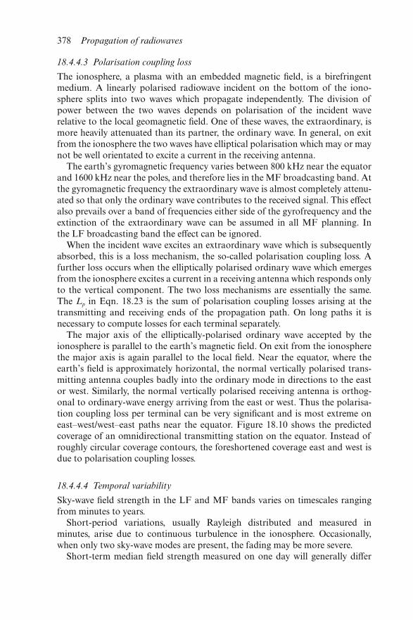
18.4.4.3 Polarisation coupling loss
The ionosphere, a plasma with an embedded magnetic field, is a birefringentmedium. A linearly polarised radiowave incident on the bottom of the iono-sphere splits into two waves which propagate independently. The division ofpower between the two waves depends on polarisation of the incident waverelative to the local geomagnetic field. One of these waves, the extraordinary, ismore heavily attenuated than its partner, the ordinary wave. In general, on exitfrom the ionosphere the two waves have elliptical polarisation which may or maynot be well orientated to excite a current in the receiving antenna.
The earth’s gyromagnetic frequency varies between 800 kHz near the equatorand 1600 kHz near the poles, and therefore lies in the MF broadcasting band. Atthe gyromagnetic frequency the extraordinary wave is almost completely attenu-ated so that only the ordinary wave contributes to the received signal. This effectalso prevails over a band of frequencies either side of the gyrofrequency and theextinction of the extraordinary wave can be assumed in all MF planning. Inthe LF broadcasting band the effect can be ignored.
When the incident wave excites an extraordinary wave which is subsequentlyabsorbed, this is a loss mechanism, the so-called polarisation coupling loss. Afurther loss occurs when the elliptically polarised ordinary wave which emergesfrom the ionosphere excites a current in a receiving antenna which responds onlyto the vertical component. The two loss mechanisms are essentially the same.The Lp in Eqn. 18.23 is the sum of polarisation coupling losses arising at thetransmitting and receiving ends of the propagation path. On long paths it isnecessary to compute losses for each terminal separately.
The major axis of the elliptically-polarised ordinary wave accepted by theionosphere is parallel to the earth’s magnetic field. On exit from the ionospherethe major axis is again parallel to the local field. Near the equator, where theearth’s field is approximately horizontal, the normal vertically polarised trans-mitting antenna couples badly into the ordinary mode in directions to the eastor west. Similarly, the normal vertically polarised receiving antenna is orthog-onal to ordinary-wave energy arriving from the east or west. Thus the polarisa-tion coupling loss per terminal can be very significant and is most extreme oneast–west/west–east paths near the equator. Figure 18.10 shows the predictedcoverage of an omnidirectional transmitting station on the equator. Instead ofroughly circular coverage contours, the foreshortened coverage east and west isdue to polarisation coupling losses.
18.4.4.4 Temporal variability
Sky-wave field strength in the LF and MF bands varies on timescales rangingfrom minutes to years.
Short-period variations, usually Rayleigh distributed and measured inminutes, arise due to continuous turbulence in the ionosphere. Occasionally,when only two sky-wave modes are present, the fading may be more severe.
Short-term median field strength measured on one day will generally differ
378 Propagation of radiowaves
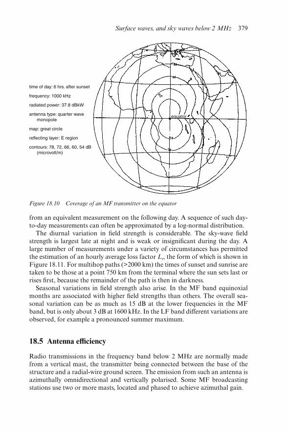
from an equivalent measurement on the following day. A sequence of such day-to-day measurements can often be approximated by a log-normal distribution.
The diurnal variation in field strength is considerable. The sky-wave fieldstrength is largest late at night and is weak or insignificant during the day. Alarge number of measurements under a variety of circumstances has permittedthe estimation of an hourly average loss factor Lt, the form of which is shown inFigure 18.11. For multihop paths (>2000 km) the times of sunset and sunrise aretaken to be those at a point 750 km from the terminal where the sun sets last orrises first, because the remainder of the path is then in darkness.
Seasonal variations in field strength also arise. In the MF band equinoxialmonths are associated with higher field strengths than others. The overall sea-sonal variation can be as much as 15 dB at the lower frequencies in the MFband, but is only about 3 dB at 1600 kHz. In the LF band different variations areobserved, for example a pronounced summer maximum.
18.5 Antenna efficiency
Radio transmissions in the frequency band below 2 MHz are normally madefrom a vertical mast, the transmitter being connected between the base of thestructure and a radial-wire ground screen. The emission from such an antenna isazimuthally omnidirectional and vertically polarised. Some MF broadcastingstations use two or more masts, located and phased to achieve azimuthal gain.
Figure 18.10 Coverage of an MF transmitter on the equator
Surface waves, and sky waves below 2 MHz 379
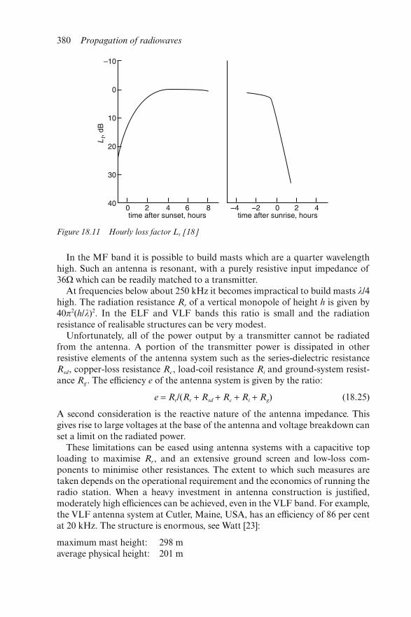
In the MF band it is possible to build masts which are a quarter wavelengthhigh. Such an antenna is resonant, with a purely resistive input impedance of36Ω which can be readily matched to a transmitter.
At frequencies below about 250 kHz it becomes impractical to build masts λ/4high. The radiation resistance Rr of a vertical monopole of height h is given by40π2(h/λ)2. In the ELF and VLF bands this ratio is small and the radiationresistance of realisable structures can be very modest.
Unfortunately, all of the power output by a transmitter cannot be radiatedfrom the antenna. A portion of the transmitter power is dissipated in otherresistive elements of the antenna system such as the series-dielectric resistanceRsd, copper-loss resistance Rc, load-coil resistance Ri and ground-system resist-ance Rg. The efficiency e of the antenna system is given by the ratio:
e = Rr/(Rr + Rsd + Rc + Ri + Rg) (18.25)
A second consideration is the reactive nature of the antenna impedance. Thisgives rise to large voltages at the base of the antenna and voltage breakdown canset a limit on the radiated power.
These limitations can be eased using antenna systems with a capacitive toploading to maximise Rr, and an extensive ground screen and low-loss com-ponents to minimise other resistances. The extent to which such measures aretaken depends on the operational requirement and the economics of running theradio station. When a heavy investment in antenna construction is justified,moderately high efficiences can be achieved, even in the VLF band. For example,the VLF antenna system at Cutler, Maine, USA, has an efficiency of 86 per centat 20 kHz. The structure is enormous, see Watt [23]:
maximum mast height: 298 maverage physical height: 201 m
Figure 18.11 Hourly loss factor Lt [18]
380 Propagation of radiowaves
number of masts: 26area of the top loading: 2.25 km2
ground screen: 3300 km of copper wire
The radiation resistance of this antenna is a mere 0.15 Ω.
18.6 Surface-wave/sky-wave interactions
At short ranges from a transmitter the surface-wave mode dominates. At longranges the sky-wave mode will normally deliver the strongest signal. At inter-mediate ranges the surface wave and sky wave may be comparable and theinterference between the two will lead to a region of signal peaks and troughs.Unlike the sky wave, the surface wave has a stable phase. Diurnal and short-termvariations in the height and structure of the lower ionosphere cause the signalpeaks and troughs to shift position. Gross variations in the sky-wave signalstrength causes the region of interplay between the two modes to move towardsor away from the transmitter.
For the long wavelengths of the VLF/LF bands the surface-wave/sky-waveinteraction gives rise to the relatively stable Hollingworth pattern referred to inSection 18.4.3. The systems required to operate in the interference region mustbe designed to function within the minima of the pattern.
In the MF band the region of interaction is called the night fading zone(NFZ). The location of the NFZ depends on any factor which affects the rela-tive amplitude of the surface and sky waves, e.g. antenna vertical radiationpattern, time of night, ground conductivity and polarisation. Other factors suchas radiated power have no effect. The fading is especially disruptive to broadcastreception and in planning such systems it is prudent to estimate the NFZ loca-tion. A fading zone which, night after night, resides over an important urbanarea will soon cause listeners to retune their receivers. The NFZ is usually takento be the region in which the difference between surface- and sky-wave fieldstrengths is 8 dB or less. When designing a broadcasting station so that the NFZis not too troublesome, it must be borne in mind that nighttime interferencefrom other cochannel transmitters may, in fact, have a more significant effect onthe quality of reception.
18.7 Background noise
The performance of any radio system is determined, in part, by the level ofbackground noise with which the wanted signal must compete. This can begenerated within the receiver or arrive at the receiver input terminals via theantenna. The four potential sources of background noise originate in thereceiver itself, in the galaxy, from atmospheric lightning discharges and fromman-made electrical equipment (see Chapter 2). Galactic noise will normally be
Surface waves, and sky waves below 2 MHz 381
reflected by the top side of the ionosphere at the frequencies considered here andcan be ignored. For most applications the level of receiver noise is also insignifi-cant compared with the atmospheric and man-made contributions. An excep-tion is in submarine communication where the atmospheric and above-surfaceman-made noise contributions may be both heavily attenuated by the sea so thatthe receiver noise contribution becomes dominant. Chapter 2 also discusses thecharacteristics of radio noise.
18.8 Acknowledgments
Parts of the text in this Chapter concerning sky-wave propagation are based onmaterial originally written by Dr. Philip Knight [24] for a previous edition ofthis book. Figures 18.9 and 18.11 are used with the kind permission of the ITUas copyright holder.
18.9 References
1 SOMMERFELD, A.: ‘The propagation of waves in wireless telegraphy’,Ann. Phys., 1909, 28, p.665
2 NORTON, K.A.: ‘The propagation of radio waves over the surface of theEarth and in the upper atmosphere. Part 1’, Proc. Inst. Radio. Eng., 1936,24, pp.1367–1387
3 NORTON, K.A.: ‘The propagation of radio waves over the surface of theEarth and in the upper atmosphere. Part 2’, Proc. Inst. Radio. Eng., 1937,25, pp. 1203–1236
4 NORTON, K. A.: ‘The calculation of ground-wave field intensity overa finitely conducting spherical Earth’, Proc. Inst. Radio Eng., 1941, 29,pp.623–639
5 VAN DER POL, B., and BREMMER, H.: ‘The diffraction of electro-magnetic waves from an electrical point source round a finitely conductingsphere’, Philos. Mag. Ser. 7, 1937, 24, pp.141–176
6 VAN DER POL, B., and BREMMER, H.: ‘The diffraction of electro-magnetic waves from an electrical point source round a finitely conductingsphere’, Philos. Mag. Ser. 7, 1937, 24, pp.825–864
7 VAN DER POL, B., and BREMMER, H.: ‘The diffraction of electro-magnetic waves from an electrical point source round a finitely conductingsphere’, Philos. Mag. Ser. 7, 1938, 25, pp.817–834
8 VAN DER POL, B., and BREMMER, H.: ‘The diffraction of electro-magnetic waves from an electrical point source round a finitely conductingsphere’, Philos. Mag. Ser. 7, 1939, 26, pp.261–275
9 BREMMER, H.: ‘Terrestrial radio waves’ (Elsevier, 1949)10 ROTHERAM, A.S.: ‘Ground-wave propagation. Part 1 Theory for short
distances’, IEE Proc. F, 1981, 128, pp.275–28411 ROTHERAM, A.S.: ‘Ground-wave propagation. Part 2 Theory for
medium and long distances and reference propagation curves’, IEE Proc. F,1918, 128, pp.285–295
382 Propagation of radiowaves

12 ROTHERAM, A.S.: ‘Ground-wave propagation’, Marconi Rev., 1982, 45,(1), pp.18–48
13 ITU-R Recommendation P.368-7: ‘Ground-wave propagation curves forfrequencies between 10 kHz and 30 MHz’, 1994
14 ITU-R Recommendation P.341-5: ‘The concept of transmission loss forradio links’, 1999
15 ITU-R Recommendation P.832-2: ‘World atlas of ground conductivities’,1999
16 MILLINGTON, G., and ISTED, G.A.: ‘Ground-wave propagation over aninhomogeneous Earth. Part 2 Experimental evidence and practical implica-tions’, Proc. IEE, 1950, 97, pp.209–222
17 CAUSEBROOK, J.H.: ‘Medium-wave propagation in built-up areas’, Proc.IEE, 1978, 125, pp.804–808
18 ITU-R Recommendation P.1147: ‘Prediction of sky-wave field strength atfrequencies between 150 and 1700 kHz’, 1999
19 ITU-R Recommendation P.684-2: ‘Prediction of field strength at frequen-cies below about 500 kHz’, 2001
20 WAIT, J. R.: ‘Electromagnetic waves in stratified media’ (Pergamon Press,New York, 1962)
21 FERGUSON, J.A.: ‘Status of the naval ocean systems long wave propaga-tion capability “LWPC”’.Paper presented at Third Workshop on ELF/VLFRadio Noise, Stanford University, USA, 1988
22 BRACEWELL, R.N., et al.: ‘The ionospheric propagation of low- andvery-low-frequency radio waves over distances less than 1000 km’, Proc.IEE, 1951, 98, Part III, pp. 221–236
23 WATT, A.D.: ‘VLF Radio Engineering’ (Pergamon Press, New York, 1967)24 KNIGHT, P., in HALL, M.P., and BARCLAY, L.W.: ‘Radiowave propaga-
tion’, IEE Electromagnetic Waves Series 30 (Peter Peregrinus, London,1989)
Surface waves, and sky waves below 2 MHz 383

Chapter 19
Terrestrial line-of-sight links:Recommendation ITU-R P.530
R.G. Howell
19.1 Introduction
Recommendation ITU-R P.530 [1] presents propagation data for planningterrestrial line-of-sight radio systems, typically operating in frequency bandsbetween 1 GHz and 45 GHz, and gives step-by-step methods for predictingthe performance of these systems for percentage times down to 0.001 per cent.The recommendation deals only with effects related to the wanted signal. Theinterference aspects of terrestrial line-of-sight link design are covered inRecommendation ITU-R P.452 [2].
Although the prediction methods presented in Recommendation ITU-RP.530 are based on the physics of radio propagation, measured data was usedas the main foundation and the majority of the formulae are semi-empiricalstatistical relationships.
The Recommendation divides broadly into methods for determining theantenna heights (with and without antenna height diversity) and methods forcalculating the statistics of signal fading, enhancement and depolarisation. Inthe case of clear air effects the methods are subdivided into a quick (initialplanning) method and a more detailed method, which requires terrain data forthe area of the link.
Other topics covered are: the correlation of simultaneous fading on multihoplinks, the frequency and polarisation scaling of rain attenuation statistics, thestatistics of rain fade duration and the prediction of the error performance andavailability of digital systems.
19.2 Overview of propagation effects
The main propagation effects that must be considered in the design of terrestrialline-of-sight links are:
• free-space loss
• attenuation due to atmospheric gases
• diffraction fading due to obstruction of the radio path by the terrain orobstacles on the terrain
• signal fading and signal enhancement due to atmospheric refractive effects
• signal fading due to multipath arising from surface reflection
• attenuation due to precipitation or solid particles in the atmosphere
• variation of the angle-of-arrival at the receive antenna and angle-of-launch atthe transmit antenna due to atmospheric refraction
• reduction in the system cross-polar performance in multipath or precipitationconditions
• signal distortion due to frequency selective fading and delay during multipathpropagation.
The free-space loss and the losses produced by dry air and water vapour havebeen described in Chapters 2 and 7. Further details on the losses produced byatmospheric gases can be found in Recommendation ITU-R P.676 [3]. The fol-lowing sections will discuss the other propagation effects having an impact onthe link design and methods for predicting the performance of a link takingaccount of these effects.
19.3 Link design
19.3.1 General
The performance of a link cannot be determined until all the relevant linkparameters, e.g. frequency, path length, antenna heights, meteorological factorsfor the area etc., are known. Therefore, the design of a link is an iterative processin which an initial design is examined and then, if necessary, changed until,hopefully, a design which meets the required performance objectives is achieved.
In a practical situation the general location, direction and capacity of the linkare the primary (fixed) requirements. The main variables in the link design arethe frequency band available, the locations of the link end points (usuallydetermined by the location of suitable high points with a clear view in therequired directions and the availability of sites for which planning consents canbe obtained), the height, number and gains of the antennas, the transmitterpowers and the receiver sensitivities and noise figures.
The constraint on the general location of the link determines the meteoro-logical factors e.g. the incidence of extreme clear air radio refractive effects andthe incidence of high rainfall rates. The constraints on the location of the end
386 Propagation of radiowaves
points then determines, at least initially, the path length and the terrain type andprofile over which the radio path must pass.
Having chosen the frequency band and the end points of the link, the mainfactors determining the link design then relate to the antennas (number, heightsand gains), transmitter powers and receiver characteristics (sensitivity andnoise figure). Given the constraints on transmitter power required to avoidinterference to other systems and the practical limitations on the receivercharacteristics, the link design then centres around:
• Achieving sufficient clearance of the radio path above the terrain such thatany losses produced by the terrain (e.g. due to diffraction) are within accept-able limits, both under average clear air conditions and during conditionsof abnormal atmospheric radio refractivity (e.g. under conditions ofsubrefraction).
• Determining the frequency separation and/or antenna spacing and/or angu-lar separation if diversity is required to achieve the required performance (seeSection 19.5).
Having carried out the initial link design and estimated its performance it maybe that, even with fading mitigation methods (see Section 19.5), the design targetis not achieved and new link end points, or a different frequency band, must beconsidered.
19.3.2 Path clearance
19.3.2.1 Nondiversity case
Two basic concepts are relevant to the determination of path clearance. The firstis the bending of the radio beam produced by variations in the radio refractiveindex of the atmosphere with height (see Chapter 7) and the second is that ofFresnel zones enclosing the path (see Chapters 3 and 8).
It was shown in Chapter 7 that the decrease in radio refractive index withincreasing height under average clear air conditions bends the radio path down-wards with a curvature that is less than that of the earth’s surface. Hence, a plotof the path over the earth’s surface results in a curved radio path over a curvedterrain profile. Transforming this plot so as to change the curved radio path intoa straight line results in a flatter terrain profile (i.e. an increased earth radius)and this transformation is often used to simplify the task of determining theclearance of the radio path over the terrain. The factor by which the earth’sradius must be multiplied to achieve this (the k factor) is typically about 4/3 (seeFigure 19.1). When designing a terrestrial line-of-site link radio refractive index,changes in the lowest 100 m of the atmosphere are of the most significance indetermining the k factor to be used.
If, instead of decreasing with height, the radio refractive index increases (ascan happen under atmospheric conditions occurring for about 0.1 per cent ofthe worst month), the radio path curves upwards and to produce a path which is
Terrestrial line-of-sight links: Recommendation ITU-R P.530 387
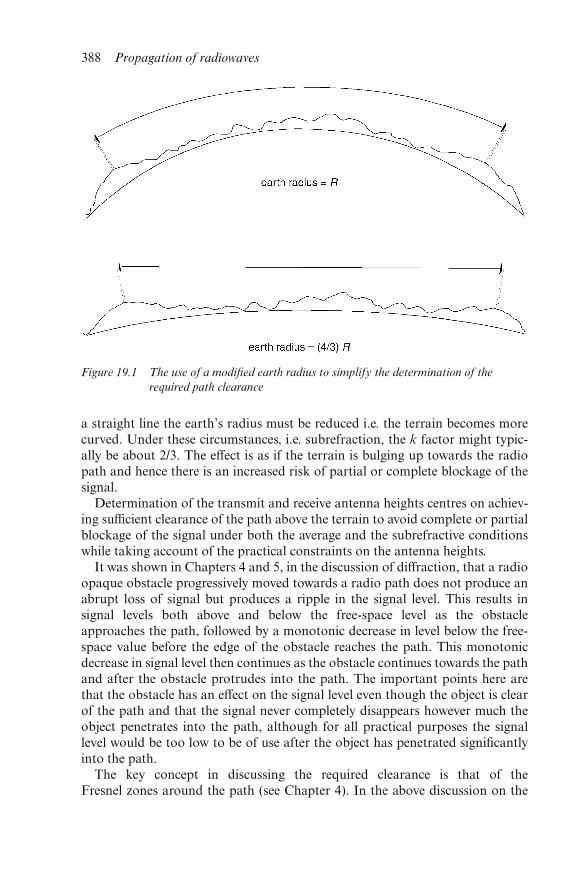
a straight line the earth’s radius must be reduced i.e. the terrain becomes morecurved. Under these circumstances, i.e. subrefraction, the k factor might typic-ally be about 2/3. The effect is as if the terrain is bulging up towards the radiopath and hence there is an increased risk of partial or complete blockage of thesignal.
Determination of the transmit and receive antenna heights centres on achiev-ing sufficient clearance of the path above the terrain to avoid complete or partialblockage of the signal under both the average and the subrefractive conditionswhile taking account of the practical constraints on the antenna heights.
It was shown in Chapters 4 and 5, in the discussion of diffraction, that a radioopaque obstacle progressively moved towards a radio path does not produce anabrupt loss of signal but produces a ripple in the signal level. This results insignal levels both above and below the free-space level as the obstacleapproaches the path, followed by a monotonic decrease in level below the free-space value before the edge of the obstacle reaches the path. This monotonicdecrease in signal level then continues as the obstacle continues towards the pathand after the obstacle protrudes into the path. The important points here arethat the obstacle has an effect on the signal level even though the object is clearof the path and that the signal never completely disappears however much theobject penetrates into the path, although for all practical purposes the signallevel would be too low to be of use after the object has penetrated significantlyinto the path.
The key concept in discussing the required clearance is that of theFresnel zones around the path (see Chapter 4). In the above discussion on the
Figure 19.1 The use of a modified earth radius to simplify the determination of the
required path clearance
388 Propagation of radiowaves
penetration of the obstacle into the path, significant could be considered as thepoint at which the obstacle penetrates more than about one Fresnel zone intothe path.
It should be noted that the shape of the edge of the obstacle has a verysignificant effect on the diffraction loss. For example, with the path just grazingthe edge of a sharp obstacle (e.g. a knife edge) the diffraction loss is about 6 dBcompared with about 15 dB for an object having a large radius of curvature (e.g.a smooth earth surface). A clearance of about 60 per cent of the first Fresnelzone is required to achieve a free-space signal level.
In the method given in Recommendation ITU-R P.530 transmit and receiveantenna heights are determined which, under average refractivity conditions(k = 4/3), give a clearance above the most significant obstacle for the whole ofthe first Fresnel zone. Then, the antenna heights required to give a clearanceof a fraction (varying between 0 and 0.6, depending on the climate and the typeof obstruction) of the first Fresnel zone for the conditions of subrefractionlikely to occur for 0.1 per cent of the worst month are determined. The value ofk to be used for the subrefractive condition (an effective k value ke) should bedetermined from radio refractivity data averaged along the path and hence it isdependent on the path length. The effective k value, as a function of path length,is given in Recommendation ITU-R P.530 in the form of a graph. Finally, havingdetermined the transmit and receive antenna heights for the above two condi-tions, the larger of the two pairs of values is chosen.
Larger path clearances than those determined by the above method for theworst month subrefractive condition may be necessary for frequencies above10 GHz in order to reduce the risk of diffraction loss during conditions of sub-refraction. Therefore, the diffraction loss should be calculated for this condition(e.g. using k = 2/3 and the methods given in Chapter 8) and, if necessary, theantenna heights increased.
Having determined the required antenna heights the link performance, takingaccount of the propagation conditions along the path, can now be estimated. Ifthe performance target cannot be achieved using single antennas at each end ofthe link the improvement provided by various mitigation techniques can beexamined (see Section 19.5).
19.3.2.2 Height diversity case
A method of reducing the link outage if the performance target cannot beachieved using single antennas is to use two vertically spaced antennas at one orboth ends of the link, i.e. using height diversity. The principle behind the use ofheight diversity is that if the variation of signal strength with height is examinedduring multipath fading, peaks and troughs are observed. Hence, with suitableantenna spacing, a trough at one antenna will coincide with a peak at the otherantenna and, with an appropriate signal combining mechanism, the system willsuffer less overall fading. Furthermore, by pointing the two antennas at slightlydifferent angles of elevation a further advantage can be obtained from the
Terrestrial line-of-sight links: Recommendation ITU-R P.530 389
variations in the angle of arrival of the signal at the two antennas (angle diver-sity) i.e. when the angle of arrival at one antenna is not optimum (not onboresight) it may be closer to optimum at the other. Therefore, the design task isto determine a suitable spacing and angular offset between the two antennas.
In the method given in Recommendation ITU-R P.530 the initial height of theupper antenna is determined by the method described in Section 19.3.2.1. It maybe necessary to change this height after determining the link outage probabilitywith diversity. The height of the second (lower) antenna is that which gives apath clearance, under median k value conditions, of between 0.6 and 0.3 of thefirst Fresnel zone for path obstructions extending along a portion of the pathand between 0.3 and 0 if there are only one or two isolated obstacles. In theabsence of a measured median value for k a value of 4/3 should be used. Alter-natively, the clearance of the lower antenna may be chosen to give about 6 dB ofdiffraction loss during normal refractivity conditions, or some other lossappropriate to the fade margin of the system.
If, after calculating the link outage with the antenna spacing derived above,the link performance is still not satisfactory some further improvement may beobtained by increasing the height of the upper antenna and/or adjusting theangular offset between the two antennas. Methods for calculating the improve-ment given by these methods are given in Recommendation ITU-R P.530.
19.4 Prediction of system performance
19.4.1 Propagation in clear air
The physical basis for the effects on radio propagation of variations in theatmospheric radio refractive index in clear air are discussed in detail in Chapter7. In this Section an overview of the methods given in Recommendation ITU-RP.530 for determining the statistics of signal fading and enhancement producedby these effects is given. The reader is referred to the Recommendation for thedetails of the step-by-step algorithms and graphical methods.
19.4.1.1 Multipath fading on a single hop of a link
Two methods are given in Recommendation ITU-R P.530 for predicting thestatistics of multipath fading on a single hop of a link:
(i) a quick method, suitable for planning applications, which does not requiredetailed information on the terrain;
(ii) a more detailed method which requires the standard deviation (sa) of theterrain heights in the region of the path.
Both methods require the point refractivity gradient in the lowest 65 m of theatmosphere not exceeded for one per cent of an average year (dN1 N km−1). Ifmeasured point refractivity data for the region of the link is not available dN1
can be obtained from Recommendation ITU-R P.453 [4].
390 Propagation of radiowaves
These two methods are further sub-divided into:
• a method applicable to the small percentage time/deep-fading (> about 25 dB)region of the distribution;
• a method applicable to all percentage times and fade depths down to 0 dB.
First, the fading statistics for an average worst month are determined and then,if necessary, these can be used to derive statistics for an average year.
The key parameter used in all the methods is a geoclimatic factor K applicableto an average worst month. Formulae for calculating this from dN1 and, in thecase of the detailed method from sa in addition to dN1, are given. Alternatively, amethod for deriving K from measured fading data is given in Appendix 1 to theRecommendation.
In the method applicable to the small percentage time/deep-fading region ofthe distribution K is used, in conjunction with the link path length (d km), thepath inclination, the frequency and the altitude of the lower of the twoantennas, to calculate directly the percentage time pw that a fade of a given depthA dB is exceeded in an average worst month.
In the method applicable to all percentage times the deep-fading distributionderived above is combined with an interpolated distribution covering fadedepths down to 0 dB. First, a multipath occurrence factor p0 is calculated, whichis then used to determine the fade depth at which the transition between thedeep-fading distribution and the shallow-fading distribution occurs. For fadedepths greater than this value the small percentage time/deep-fading distribu-tion is used. For fade depths less than the transition value an interpolationprocedure is given.
In both cases either a step-by-step algorithmic method or a graphical methodcan be used (the required graphs are given in the Recommendation). Anapproximate value for the lower frequency limit for which the methods are validis given by 15/d GHz.
19.4.1.2 Simultaneous clear-air fading on multihop links
Measurements indicate that, in clear-air conditions, fading events exceeding20 dB on adjacent hops of a multihop link are almost completely uncorrelated.This suggests that, for analogue systems with large fade margins, the outage timefor a series of hops in tandem is approximately given by the sum of the outagetimes for the individual hops.
For fade depths not exceeding 10 dB, the probability of simultaneouslyexceeding a given fade depth on two adjacent hops can be estimated from:
P12 = (P1 P2)0.8 (19.1)
where P1 and P2 are the probabilities of exceeding this fade depth on eachindividual hop.
The correlation between fading on adjacent hops decreases with increasingfade depth between 10 dB and 20 dB, so that the probability of simultaneously
Terrestrial line-of-sight links: Recommendation ITU-R P.530 391
exceeding a fade depth of greater than 20 dB can be approximately expressedby:
P12 = P1 P2 (19.2)
19.4.1.3 Signal level enhancement
Large signal level enhancements can occur during the same general conditionsthat result in multipath fading. A procedure, similar to that described abovecovering fading for all percentage times, is used to determine the distribution ofsignal level enhancement.
First, a distribution valid for enhancements greater than 10 dB, and derivedusing the fade depth exceeded for 0.01 per cent of the average worst month(using the methods described above), is produced. Then, using an interpolationprocedure, the distribution of enhancements between 10 dB and 0 dB isobtained and combined with the distribution for enhancements greater than10 dB to obtain a distribution covering all enhancement levels.
19.4.1.4 Conversion from average worst month to average annual distributions
It should be noted that the methods discussed above for predicting clear airsignal fading and enhancement give statistics for the average worst month. Insome cases link performance criteria are specified in terms of both average worstmonth and average annual percentage times. Therefore, methods for convertingfrom the average worst month distribution to the average annual distribution areof use to the link designer. Recommendation ITU-R P.530 provides methods forcarrying out this conversion.
The annual distribution is obtained by combining two distributions, onederived from the deep-fading range of the average worst month distribution andthe other derived from the shallow-fading range of the average worst monthdistribution. In the deep-fading range a logarithmic geoclimatic conversion fac-tor ΔG, which is a function of the link latitude, path length and path inclination,is used to derive the average annual percentage time p from the average worstmonth percentage time pw.
Methods are also given in the Recommendation for the conversion of theaverage worst month distributions of fading to shorter worst periods in therange from 1 h to 720 h and for the conversion of the average worst monthenhancement distribution to an average annual enhancement distribution.
19.4.1.5 Reduction of system cross-polar performance due to clear air effects
Cross-polar discrimination (XPD) is a measure of the separation betweenorthogonally (typically vertical and horizontal) polarised signals that can beachieved by an antenna. A reduction in the XPD of an antenna (for example,produced by off-axis reception or transmission) can result in cochannel interfer-ence and, to a lesser extent, adjacent channel interference. The effect of multi-path propagation on the arrival or transmission angle of signals combined with
392 Propagation of radiowaves
the antenna cross-polar patterns determines the reduction in the system XPDfor small percentage times and clear-air propagation conditions.
A method for estimating the probability of outage due to this effect is given inRecommendation ITU-R P.530. The method is based on a multipath activityparameter which is closely related to the frequency of occurrence of multipathin an average worst month. This is then used to calculate the probability ofoutage, taking into account the number of antennas and their spacing (in thecase of space diversity) and, if used, the effect of cross-polar cancellation (seeSection 19.5.3).
19.4.2 Propagation in rain
19.4.2.1 Attenuation by rain
The physics of attenuation by rain has been discussed in detail in Chapter 12.This Section presents an overview of the method given in RecommendationITU-R P.530 for predicting the long-term statistics of rain attenuation.
The primary input to the procedure is the rainfall rate R0.01 (mm h−1), averagedover a period of 1 min and exceeded for 0.01 per cent of the time for the regionof the link. If this information cannot be obtained from long-term measure-ments carried out in the location of the link an estimate can be obtained fromrainfall rate maps given in Recommendation ITU-R P.837 [5].
An effective path length, which is less than the actual path length and whichreduces with increasing value of R0.01, is calculated. This takes account of thenonuniformity of the rainfall rate along the path, particularly for high rainfallrates e.g. >20 mm h−1.
An estimate of the path attenuation exceeded for 0.01 per cent of the time isthen obtained by multiplying the effective path length by the rain-specificattenuation (dB km−1) for a rainfall rate of R0.01 mm h−1. The rain-specific attenu-ation is given in Recommendation ITU-R P.838 [6] as a function of frequency,polarisation and rainfall rate.
Two formulae are given in the recommendation for deriving the path attenu-ation exceeded for percentage times in the range 1 to 0.001 per cent from the 0.01per cent value. One applies to links between 30° north and 30° south and theother applies to links outside this region.
It should be noted that the propagation model described above gives the rainattenuation statistics for an average year. System planning often requires statis-tics for an average worst month. These can be derived from the average annualstatistics using methods given in Recommendation ITU-R P.841 [7].
At frequencies where both rain attenuation and multipath fading must betaken into account the exceedance percentages for a given fade depth corre-sponding to each of these mechanisms can be added.
19.4.2.2 Frequency and polarisation scaling of rain attenuation statistics
When reliable long-term rain attenuation statistics are available at one frequency
Terrestrial line-of-sight links: Recommendation ITU-R P.530 393
(f1) an estimate of the statistics for a link operating at another frequency (f2),having the same hop length and in the same climate, can be made using therelationship:
A2 = A1 (Φ2/Φ1)1 − H (19.3)
where
Φ( f) = f 2
1 + 10−4 f 2(19.4)
H = 1.12 × 10⁻³(Φ2/Φ1)0.5(Φ1A1)
0.55 (19.5)
and A1 and A2 are the equiprobable values of the excess rain attenuation atfrequencies f1 and f2 (GHz), respectively.
Similarly, when reliable long-term rain attenuation statistics are available for alink, either for vertical (V) or horizontal (H) polarisation, the attenuation statis-tics for the same frequency and the same link, but for the other polarisation, maybe estimated using the relationships:
AV = 300AH
335 + AH
(19.6)
or
AH = 335AV
300 + AV
(19.7)
where AV and AH are equiprobable values in dB.
19.4.2.3 Statistics of the number and duration of rain fades
There is strong evidence that the duration of rain fades is much longer than thatof multipath fades. If an event is defined to be the exceedance of attenuation A(dB) for a given period of time (τ) or longer then the relationship between thenumber of fades Nτ(A) and A is given by:
Nτ(A) = a Ab (19.8)
where a and b are coefficients that are expected to depend on frequency, pathlength and other variables such as climate. Measurements carried out in Scandi-navia on a 15 km path at 18 GHz for a one-year period indicate that for τ = 10 s,a = 5.7 × 10⁵ and b = −3.4.
If T(A) is the total time for which an attenuation of A dB is exceeded andDm(A) is the mean duration of the fades contributing to this total time then:
Dm(A) = T(A)/Nτ(A) (19.9)
19.4.2.4 Rain fading on multihop links
If the occurrence of rainfall were statistically independent of location, then theoverall probability of fading PT for a linear series of hops in tandem would be
394 Propagation of radiowaves
given to a good approximation by summing the individual probabilities i.e.:
PT =�n
i=1
Pi (19.10)
where Pi is probability for the ith of the total of n hops.Alternatively, if rain events are correlated over distances comparable to two or
more hops in tandem then the combined fading probability for a multihop linkis given by:
PT = K �n
i = 1
Pi (19.11)
where K is a factor (<1) that includes the effect of the spatial correlation ofthe rainfall and is a function of the general orientation of the link relative to theprevailing direction of rainstorms in the area, the hop length, the total numberof hops and the percentage exceedance time of interest. Graphs, giving a seriesof curves for K, are given in Recommendation ITU-R P.530.
19.4.2.5 Depolarisation by rain
The polarisation state of signals transmitted through rain may be changedbecause of the nonspherical shape of large raindrops in heavy rain (see Chapter12). This reduces the cross-polar discrimination (XPD) of the system and maycause outage due to cochannel interference and, to a lesser extent, adjacentchannel interference. The effect is least for vertically or horizontally polarisedsignals (the normal case for terrestrial line-of-sight links) and greatest for lin-early polarised signals at 45° to the horizontal or for circularly polarised signals.However, some reduction of XPD still occurs even for vertically or horizontallypolarised signals due to the tilting of the axis of symmetry of the raindrops awayfrom the vertical produced by wind shear near the ground.
Recommendation ITU-R P.530 gives a method for estimating the statistics ofXPD from those of the attenuation measured on the link. The basis of themethod is the relationship observed between the equiprobable values ofXPD and copolar attenuation (CPA) derived from concurrent long-termmeasurements. This takes the form:
XPD = U − V( f ) log CPA (19.12)
where
U = U0 + 30 log f (19.13)
and
V( f ) = 12.8 f 0.19 for 8 ≤ f ≤ 20 GHz (19.14)
V( f ) = 22.6 for 20 < f ≤ 35 GHz (19.15)
A mean value for U0 of about 15 dB (with a lower bound of 9 dB) is suggestedfor fades in excess of 15 dB.
Terrestrial line-of-sight links: Recommendation ITU-R P.530 395
19.5 Mitigation methods
The effects of slow, relatively nonfrequency selective clear-air fading (i.e. flatfading) due to beam spreading, and the faster frequency-selective clear-airfading due to multipath propagation can be reduced by both nondiversityand diversity techniques.
19.5.1 Techniques without diversity
Several methods can be employed to reduce the effects of multipath fadingwithout the need for diversity. These are:
(a) Reducing the level of ground reflections: links should be sited where possibleto reduce surface reflections, thus reducing the occurrence of multipathfading and distortion. Techniques for achieving this include the siting ofthe ends of over-water links at locations which place surface reflections onland rather than water and the siting of over-land and over-water links soas to avoid large flat highly reflecting surfaces on land. Another technique isto tilt the antennas upwards slightly, thus reducing the gain of the antennasin the direction of the reflection; however, in this case a trade-off must bemade between the resultant loss in effective antenna gain under normalrefractivity conditions and the reduction of multipath fading.
(b) Increasing the path inclination: links should be sited to take advantage ofthe terrain in ways that will increase the path inclination, since increasingpath inclination reduces the effects of beam spreading, surface multipathfading and atmospheric multipath fading. In addition, the positions of theantennas on the radio link towers should be chosen to give the largestpossible inclinations, particularly for the longest links.
(c) Reducing the path clearance: reducing the path clearance can reduce theincidence of multipath fading, however, a trade-off must be made betweenthe reduction in the effects of multipath fading and distortion and the riskof increased fading in conditions of subrefraction.
19.5.2 Diversity techniques
Diversity techniques include space, angle and frequency diversity. Frequencydiversity should be avoided whenever possible so as to conserve spectrum.Whenever space diversity is used, angle diversity should also be employed bytilting the antennas at different upward angles. Angle diversity can be used insituations in which adequate space diversity is not possible or to reduce towerheights.
The amount of improvement afforded by all of these techniques depends on theextent to which the signals in the diversity branches of the system are uncorre-lated. For narrowband analogue systems, it is sufficient to determine theimprovement in the statistics of fade depth at a single frequency. For wideband
396 Propagation of radiowaves
digital systems, the diversity improvement also depends on the statistics ofin-band distortion.
The diversity improvement factor, I, for a fade depth A is defined by:
I = p(A)/pd(A) (19.16)
where pd(A) is the percentage of time in the combined diversity signal branchwith a fade depth larger than A and p(A) is the percentage time for theunprotected path. The diversity improvement factor for digital systems isdefined by the ratio of the exceedance times for a given BER with and withoutdiversity.
Recommendation ITU-R P.530 gives methods for predicting the diversityimprovement factor and the outage when space diversity, frequency diversity,angle diversity and combinations of these are used.
19.5.3 Cross-polar cancellation
A method for reducing the interference that may result from the depolarisedcomponent of a signal appearing in the orthogonally polarised channel is totake a small proportion of that signal (equal in amplitude to the interference)and add it in antiphase to the signals (wanted and interference) in the orthogon-ally polarised channel. Using this technique some or all of the interference canbe cancelled out.
19.6 References
1 Recommendation ITU-R P.530-8: ‘Propagation data and predictionmethods required for the design of terrestrial line-of-sight systems’, 1999
2 Recommendation ITU-R P.452-9: ‘Prediction procedure for the evaluationof microwave interference between stations on the surface of the earth atfrequencies above about 0.7GHz’, 1999
3 Recommendation ITU-R P.676-4: ‘Attenuation by atmospheric gases’, 19994 Recommendation ITU-R P.453-7: ‘The radio refractive index: its formula
and refractivity data’, 19995 Recommendation ITU-R P.837-2: ‘Characteristics of precipitation for
propagation modelling’, 19996 Recommendation ITU-R P. 838-1: ‘Specific attenuation model for rain for
use in prediction methods’, 19997 Recommendation ITU-R P. 841-1: ‘Conversion of annual statistics to worst-
month statistics’, 1999
Terrestrial line-of-sight links: Recommendation ITU-R P.530 397

Chapter 20
The principal elements of RecommendationITU-R P.452
Tim Hewitt
20.1 Introduction
Nowadays, many new technologies and additional users are seeking access to anincreasingly busy radio spectrum. An evolving propagation and interferencemodelling capability is clearly needed to support the necessary spectrum man-agement changes and to resolve the spectrum sharing and system deploymentissues that arise within a multioperator, multiservice situation.
In the middle of the 1980s it became clear that the methods then available tomodel interference propagation at microwave frequencies would not be adequatefor the tasks which lay ahead. Considerable effort was therefore invested indevising more flexible and reliable means of predicting microwave interference.These notes provide an introduction to one such development, a new set ofpropagation models developed by a major European collaborative project(COST 210 [1]), and subsequently adopted in 1992 by ITU-R Study Group 3 asRecommendation ITU-R P.452 [2]. Since then the ITU-R Study Group hasprogressively extended the capabilities and accuracy of the original COST 210method to cope with new interference scenarios and to provide full globalapplicability.
20.2 The COST 210 approach to developing a new predictionprocedure
Clear-air interference propagation embraces a mix of propagation mechanisms,most of which involve complex interactions between the atmosphere and theearth’s surface. The distances over which interference levels can be significant(several hundred kilometres in the case of the anomalous propagation modes),
with conditions that vary with time and in different locations. It was (andremains) unrealistic to consider modelling the propagation environment on awholly theoretical basis, and semi-empirical modelling techniques had to beemployed. However, it was possible to ensure that these models addressed thecorrect physical phenomena by supporting the modelling activities, with morefundamental propagation research backed up by propagation measurements.The research programme supporting the COST210 interference prediction pro-cedure therefore comprised three complementary elements: radio meteorologicalanalysis, propagation experiments and propagation modelling.
20.3 Radio meteorological studies
These studies, which primarily addressed the clear-air effects, were undertakento identify the most important anomalous propagation mechanisms to beaddressed by the propagation models, and to indicate how their relative import-ance varied over inland, sea and coastal areas. One particular study [3] looked atthe atmospheric (rather than propagation) processes that give rise to short-terminterference propagation conditions, and resulted in models of inland, coastaland anomalous propagation which were confirmed using the measured radiodata. This work also showed how mixed (e.g. land plus sea) paths could becharacterised to determine the dominant radio meteorological conditions.
Other studies yielded data which allowed the development of a location-dependent effective earth radius (or k factor) model to allow diffractionmodelling across a range of time percentages. This model was derived from acombination of European experimental radio measurements and radiosondedata.
20.4 Propagation measurements
Experimental measurements were vital to both the development and the testingof the COST210 propagation models. A search was made for existing data, butwith limited success as very little suitable material existed even for Europe, andvirtually none existed for the remainder of the world.
Significant use was therefore made of the extensive database of measurementscompiled during the COST210 project. Altogether measured results from some64 paths (24 preCOST210, 40 during COST210) from inland, sea and coastalareas were used, covering distances of 60–1000 km and frequencies from0.7–19 GHz. Figure 20.1 shows the largest of several COST210 networks ofexperiments to emphasise the extent of the supporting measurement campaigns.
400 Propagation of radiowaves
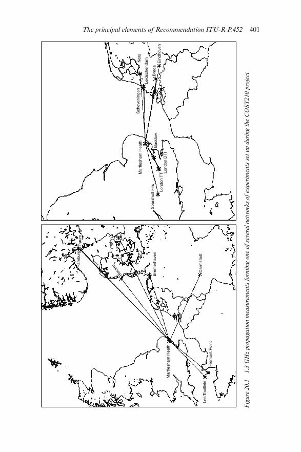
Fig
ure
20.1
1.3
GH
z pro
paga
tion m
easu
rem
ents
form
ing o
ne
of
seve
ral
net
work
s of
exper
imen
ts s
et u
p d
uri
ng t
he
CO
ST
210 p
roje
ct
The principal elements of Recommendation ITU-R P.452 401
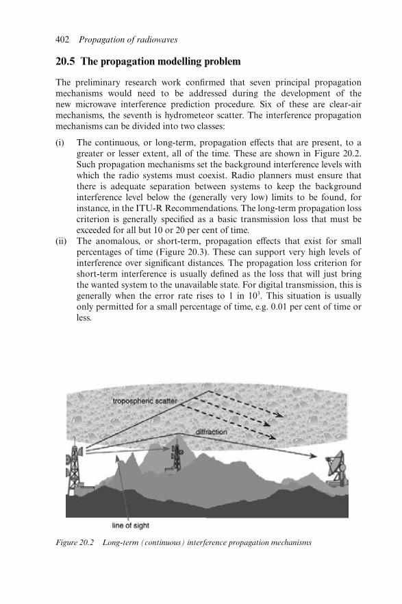
20.5 The propagation modelling problem
The preliminary research work confirmed that seven principal propagationmechanisms would need to be addressed during the development of thenew microwave interference prediction procedure. Six of these are clear-airmechanisms, the seventh is hydrometeor scatter. The interference propagationmechanisms can be divided into two classes:
(i) The continuous, or long-term, propagation effects that are present, to agreater or lesser extent, all of the time. These are shown in Figure 20.2.Such propagation mechanisms set the background interference levels withwhich the radio systems must coexist. Radio planners must ensure thatthere is adequate separation between systems to keep the backgroundinterference level below the (generally very low) limits to be found, forinstance, in the ITU-R Recommendations. The long-term propagation losscriterion is generally specified as a basic transmission loss that must beexceeded for all but 10 or 20 per cent of time.
(ii) The anomalous, or short-term, propagation effects that exist for smallpercentages of time (Figure 20.3). These can support very high levels ofinterference over significant distances. The propagation loss criterion forshort-term interference is usually defined as the loss that will just bringthe wanted system to the unavailable state. For digital transmission, this isgenerally when the error rate rises to 1 in 103. This situation is usuallyonly permitted for a small percentage of time, e.g. 0.01 per cent of time orless.
Figure 20.2 Long-term (continuous) interference propagation mechanisms
402 Propagation of radiowaves
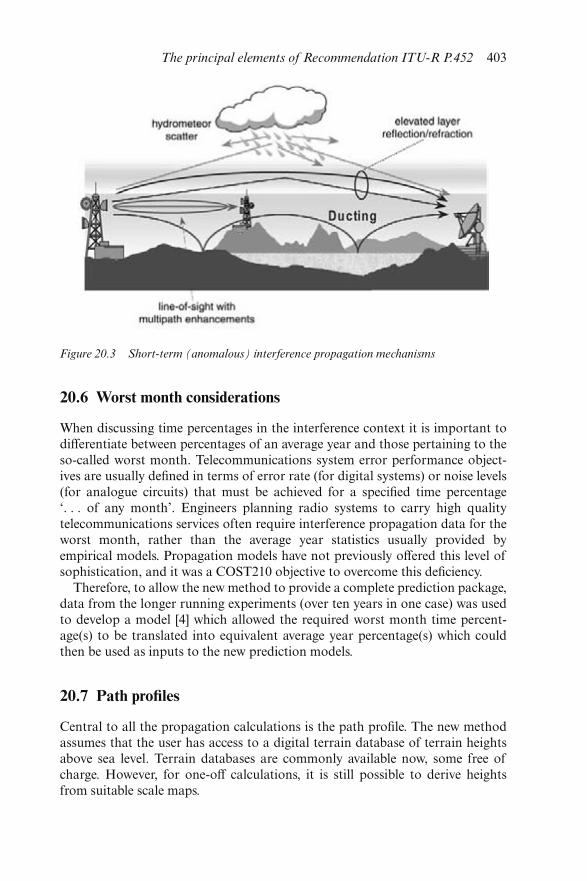
20.6 Worst month considerations
When discussing time percentages in the interference context it is important todifferentiate between percentages of an average year and those pertaining to theso-called worst month. Telecommunications system error performance object-ives are usually defined in terms of error rate (for digital systems) or noise levels(for analogue circuits) that must be achieved for a specified time percentage‘. . . of any month’. Engineers planning radio systems to carry high qualitytelecommunications services often require interference propagation data for theworst month, rather than the average year statistics usually provided byempirical models. Propagation models have not previously offered this level ofsophistication, and it was a COST210 objective to overcome this deficiency.
Therefore, to allow the new method to provide a complete prediction package,data from the longer running experiments (over ten years in one case) was usedto develop a model [4] which allowed the required worst month time percent-age(s) to be translated into equivalent average year percentage(s) which couldthen be used as inputs to the new prediction models.
20.7 Path profiles
Central to all the propagation calculations is the path profile. The new methodassumes that the user has access to a digital terrain database of terrain heightsabove sea level. Terrain databases are commonly available now, some free ofcharge. However, for one-off calculations, it is still possible to derive heightsfrom suitable scale maps.
Figure 20.3 Short-term (anomalous) interference propagation mechanisms
The principal elements of Recommendation ITU-R P.452 403
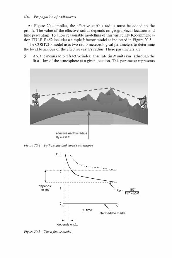
As Figure 20.4 implies, the effective earth’s radius must be added to theprofile. The value of the effective radius depends on geographical location andtime percentage. To allow reasonable modelling of this variability Recommenda-tion ITU-R P.452 includes a simple k factor model as indicated in Figure 20.5.
The COST210 model uses two radio meteorological parameters to determinethe local behaviour of the effective earth’s radius. These parameters are:
(i) ΔN, the mean radio refractive index lapse rate (in N units km−1) through thefirst 1 km of the atmosphere at a given location. This parameter represents
Figure 20.4 Path profile and earth’s curvatures
Figure 20.5 The k factor model
404 Propagation of radiowaves
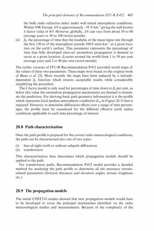
the bulk radio refractive index under well mixed atmospheric conditions.Within NW Europe ΔN is approximately −39 N km−1 giving the well knownk factor value of 4/3. However, globally, ΔN can vary from about 30 to 80(average year) or 50 to 100 (worst month).
(ii) β0, the percentage of time that the modulus of the mean lapse rate throughthe first 150 m of the atmosphere exceeds 100N units km−1 at a given loca-tion on the earth’s surface. This parameter represents the percentage oftime that fully developed clear-air anomalous propagation is deemed tooccur at a given location. β0varies around the world from 1 to 50 per cent(average year) and 2 to 90 per cent (worst month).
The earlier versions of ITU-R Recommendation P.452 provided world maps ofthe values of these two parameters. These maps were based on the original workof Bean et al. [5]. More recently the maps have been replaced by a latitude-dependent β0 function which returns acceptable results while considerablysimplifying the procedure.
The k factor model is only used for percentages of time down to β0 per cent, asbelow this value the anomalous propagation mechanisms are deemed to domin-ate the prediction. For deriving basic path geometry information it is the profilewhich represents local median atmospheric conditions (k50 in Figure 20.5) that isrequired. However, to determine diffraction effects over a range of time percent-ages, the profile must be reanalysed for the different effective earth radiusconditions applicable to each time percentage of interest.
20.8 Path characterisation
Once the path profile is prepared for the correct radio meteorological conditions,the path can be characterised into one of two types:
(i) line-of-sight (with or without subpath diffraction)(ii) transhorizon
This characterisation then determines which propagation models should beapplied to the path.
For transhorizon paths, Recommendation P.452 model provides a detailedmethod for analysing the path profile to determine all the necessary terrain-related parameters (horizon distances and elevation angles, terrain roughnessetc.).
20.9 The propagation models
The initial COST210 studies showed that new propagation models would haveto be developed to cover the principal mechanisms identified via the radiometeorological studies and measurements. Because of the complexity of the
The principal elements of Recommendation ITU-R P.452 405
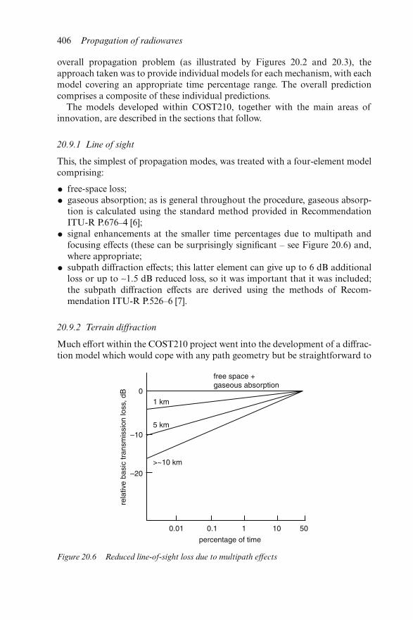
overall propagation problem (as illustrated by Figures 20.2 and 20.3), theapproach taken was to provide individual models for each mechanism, with eachmodel covering an appropriate time percentage range. The overall predictioncomprises a composite of these individual predictions.
The models developed within COST210, together with the main areas ofinnovation, are described in the sections that follow.
20.9.1 Line of sight
This, the simplest of propagation modes, was treated with a four-element modelcomprising:
• free-space loss;
• gaseous absorption; as is general throughout the procedure, gaseous absorp-tion is calculated using the standard method provided in RecommendationITU-R P.676–4 [6];
• signal enhancements at the smaller time percentages due to multipath andfocusing effects (these can be surprisingly significant – see Figure 20.6) and,where appropriate;
• subpath diffraction effects; this latter element can give up to 6 dB additionalloss or up to ∼1.5 dB reduced loss, so it was important that it was included;the subpath diffraction effects are derived using the methods of Recom-mendation ITU-R P.526–6 [7].
20.9.2 Terrain diffraction
Much effort within the COST210 project went into the development of a diffrac-tion model which would cope with any path geometry but be straightforward to
Figure 20.6 Reduced line-of-sight loss due to multipath effects
406 Propagation of radiowaves
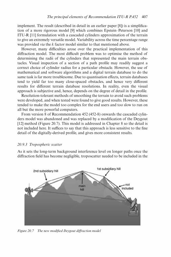
implement. The result (described in detail in an earlier paper [8]) is a simplifica-tion of a more rigorous model [9] which combines Epstein–Peterson [10] andITU-R [11] formulation with a cascaded cylinders approximation of the terrainto give an extremely versatile model. Variability across the time percentage rangewas provided via the k factor model similar to that mentioned above.
However, many difficulties arose over the practical implementation of thisdiffraction model. The most difficult problem was to optimise the method ofdetermining the radii of the cylinders that represented the main terrain obs-tacles. Visual inspection of a section of a path profile may readily suggest acorrect choice of cylinder radius for a particular obstacle. However, the use ofmathematical and software algorithms and a digital terrain database to do thesame task is far more troublesome. Due to quantisation effects, terrain databasestend to yield far too many close-spaced obstacles, and hence very differentresults for different terrain database resolutions. In reality, even the visualapproach is subjective and, hence, depends on the degree of detail in the profile.
Resolution-tolerant methods of smoothing the terrain to avoid such problemswere developed, and when tested were found to give good results. However, thesetended to make the model too complex for the end users and too slow to run onall but the more powerful computers.
From version 8 of Recommendation 452 (452-8) onwards the cascaded cylin-ders model was abandoned and was replaced by a modification of the Deygout[12] method (Figure 20.7). This model is addressed in Chapter 8 so the detail isnot included here. It suffices to say that this approach is less sensitive to the finedetail of the digitally-derived profile, and gives more consistent results.
20.9.3 Tropospheric scatter
As it sets the long-term background interference level on longer paths once thediffraction field has become negligible, troposcatter needed to be included in the
Figure 20.7 The new modified Deygout diffraction model
The principal elements of Recommendation ITU-R P.452 407
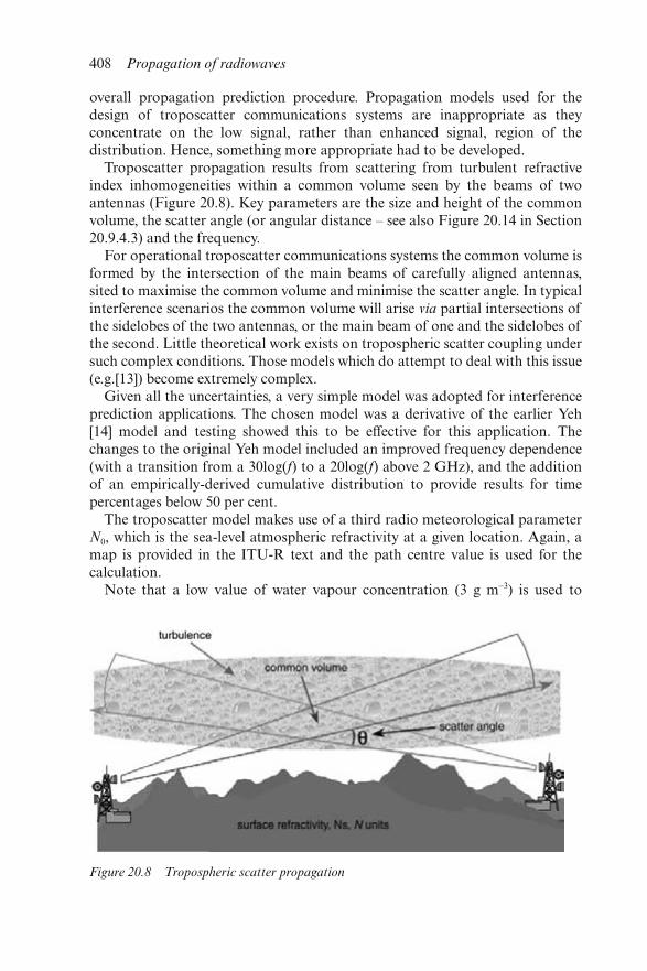
overall propagation prediction procedure. Propagation models used for thedesign of troposcatter communications systems are inappropriate as theyconcentrate on the low signal, rather than enhanced signal, region of thedistribution. Hence, something more appropriate had to be developed.
Troposcatter propagation results from scattering from turbulent refractiveindex inhomogeneities within a common volume seen by the beams of twoantennas (Figure 20.8). Key parameters are the size and height of the commonvolume, the scatter angle (or angular distance – see also Figure 20.14 in Section20.9.4.3) and the frequency.
For operational troposcatter communications systems the common volume isformed by the intersection of the main beams of carefully aligned antennas,sited to maximise the common volume and minimise the scatter angle. In typicalinterference scenarios the common volume will arise via partial intersections ofthe sidelobes of the two antennas, or the main beam of one and the sidelobes ofthe second. Little theoretical work exists on tropospheric scatter coupling undersuch complex conditions. Those models which do attempt to deal with this issue(e.g.[13]) become extremely complex.
Given all the uncertainties, a very simple model was adopted for interferenceprediction applications. The chosen model was a derivative of the earlier Yeh[14] model and testing showed this to be effective for this application. Thechanges to the original Yeh model included an improved frequency dependence(with a transition from a 30log(f) to a 20log(f) above 2 GHz), and the additionof an empirically-derived cumulative distribution to provide results for timepercentages below 50 per cent.
The troposcatter model makes use of a third radio meteorological parameterN0, which is the sea-level atmospheric refractivity at a given location. Again, amap is provided in the ITU-R text and the path centre value is used for thecalculation.
Note that a low value of water vapour concentration (3 g m−3) is used to
Figure 20.8 Tropospheric scatter propagation
408 Propagation of radiowaves
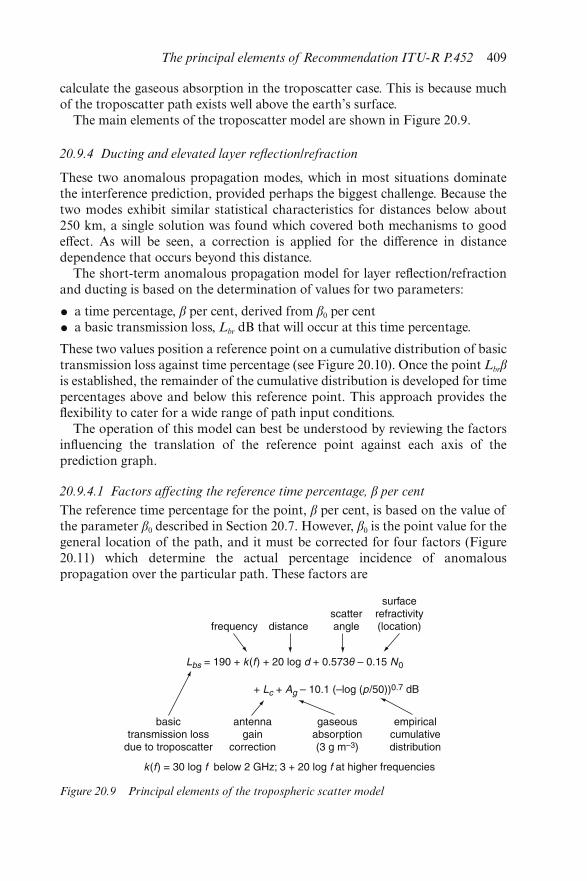
calculate the gaseous absorption in the troposcatter case. This is because muchof the troposcatter path exists well above the earth’s surface.
The main elements of the troposcatter model are shown in Figure 20.9.
20.9.4 Ducting and elevated layer reflection/refraction
These two anomalous propagation modes, which in most situations dominatethe interference prediction, provided perhaps the biggest challenge. Because thetwo modes exhibit similar statistical characteristics for distances below about250 km, a single solution was found which covered both mechanisms to goodeffect. As will be seen, a correction is applied for the difference in distancedependence that occurs beyond this distance.
The short-term anomalous propagation model for layer reflection/refractionand ducting is based on the determination of values for two parameters:
• a time percentage, β per cent, derived from β0 per cent
• a basic transmission loss, Lbr dB that will occur at this time percentage.
These two values position a reference point on a cumulative distribution of basictransmission loss against time percentage (see Figure 20.10). Once the point Lbrβ
is established, the remainder of the cumulative distribution is developed for timepercentages above and below this reference point. This approach provides theflexibility to cater for a wide range of path input conditions.
The operation of this model can best be understood by reviewing the factorsinfluencing the translation of the reference point against each axis of theprediction graph.
20.9.4.1 Factors affecting the reference time percentage, β per cent
The reference time percentage for the point, β per cent, is based on the value ofthe parameter β0 described in Section 20.7. However, β0 is the point value for thegeneral location of the path, and it must be corrected for four factors (Figure20.11) which determine the actual percentage incidence of anomalouspropagation over the particular path. These factors are
Figure 20.9 Principal elements of the tropospheric scatter model
The principal elements of Recommendation ITU-R P.452 409
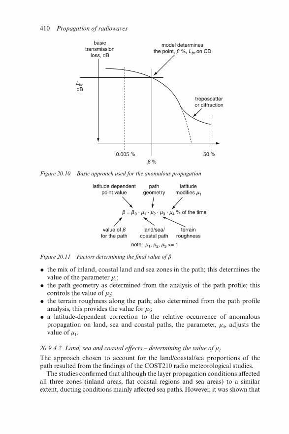
• the mix of inland, coastal land and sea zones in the path; this determines thevalue of the parameter μ1;
• the path geometry as determined from the analysis of the path profile; thiscontrols the value of μ2;
• the terrain roughness along the path; also determined from the path profileanalysis, this provides the value for μ3;
• a latitude-dependent correction to the relative occurrence of anomalouspropagation on land, sea and coastal paths, the parameter, μ4, adjusts thevalue of μ1.
20.9.4.2 Land, sea and coastal effects – determining the value of μ1
The approach chosen to account for the land/coastal/sea proportions of thepath resulted from the findings of the COST210 radio meteorological studies.
The studies confirmed that although the layer propagation conditions affectedall three zones (inland areas, flat coastal regions and sea areas) to a similarextent, ducting conditions mainly affected sea paths. However, it was shown that
Figure 20.10 Basic approach used for the anomalous propagation
Figure 20.11 Factors determining the final value of β
410 Propagation of radiowaves
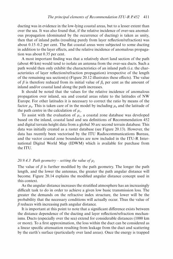
ducting was in evidence in the low-lying coastal areas, but to a lesser extent thanover the sea. It was also found that, if the relative incidence of over-sea anomal-ous propagation (dominated by the occurrence of ducting) is taken as unity,then that of inland paths (resulting purely from layer reflection/refraction) wasabout 0.15–0.2 per cent. The flat coastal areas were subjected to some ductingin addition to the layer effects, and the relative incidence of anomalous propaga-tion was about 0.35 per cent.
A most important finding was that a relatively short land section of the path(about 40 km) would tend to isolate an antenna from the over-sea ducts. Such apath would then only exhibit the characteristics of an inland path (i.e. the char-acteristics of layer reflection/refraction propagation) irrespective of the lengthof the remaining sea section(s) (Figure 20.12 illustrates these effects). The valueof β is therefore reduced from its initial value of β0 per cent as the amount ofinland and/or coastal land along the path increases.
It should be noted that the values for the relative incidence of anomalouspropagation over inland, sea and coastal areas relate to the latitudes of NWEurope. For other latitudes it is necessary to correct the ratio by means of thefactor μ4. This is taken care of in the model by including μ4 and the latitude ofthe path centre in the calculation of μ1.
To assist with the evaluation of μ1, a coastal zone database was developedbased on the inland, coastal land and sea definitions of Recommendation 452and digital terrain height data from a global 30 arc second terrain database. Thisdata was initially created as a raster database (see Figure 20.13). However, thedata has recently been vectorised by the ITU Radiocommunications Bureau,and the vector coastal zone boundaries are now included in the ITU-R Inter-national Digital World Map (IDWM) which is available for purchase fromthe ITU.
20.9.4.3 Path geometry – setting the value of μ2
The value of β is further modified by the path geometry. The longer the pathlength, and the lower the antennas, the greater the path angular distance willbecome. Figure 20.14 explains the modified angular distance concept used inthis context.
As the angular distance increases the stratified atmosphere has an increasinglydifficult task to do in order to achieve a given low basic transmission loss. Thegreater the demands on the refractive index structure, the lower will be theprobability that the necessary conditions will actually occur. Thus the value ofβ reduces with increasing path angular distance.
It is important at this point to note that a significant difference exists betweenthe distance dependence of the ducting and layer reflection/refraction mechan-isms. Ducts (especially over the sea) extend for considerable distances (1000 kmor more). To a first approximation, the loss within the duct can be considered asa linear specific attenuation resulting from leakage from the duct and scatteringby the earth’s surface (particularly over land areas). Once the energy is trapped
The principal elements of Recommendation ITU-R P.452 411
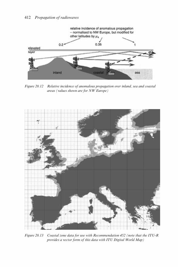
Figure 20.12 Relative incidence of anomalous propagation over inland, sea and coastal
areas (values shown are for NW Europe)
Figure 20.13 Coastal zone data for use with Recommendation 452 (note that the ITU-R
provides a vector form of this data with ITU Digital World Map)
412 Propagation of radiowaves
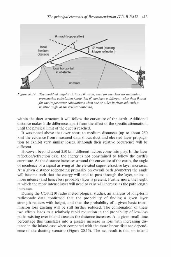
within the duct structure it will follow the curvature of the earth. Additionaldistance makes little difference, apart from the effect of the specific attenuation,until the physical limit of the duct is reached.
It was noted above that over short to medium distances (up to about 250km) the evidence from measured data shows duct and elevated layer propaga-tion to exhibit very similar losses, although their relative occurrence will bedifferent.
However, beyond about 250 km, different factors come into play. In the layerreflection/refraction case, the energy is not constrained to follow the earth’scurvature. As the distance increases around the curvature of the earth, the angleof incidence of a signal arriving at the elevated super-refractive layer increases.At a given distance (depending primarily on overall path geometry) the anglewill become such that the energy will tend to pass through the layer, unless amore intense (and hence less probable) layer is present. Furthermore, the heightat which the more intense layer will need to exist will increase as the path lengthincreases.
During the COST210 radio meteorological studies, an analysis of long-termradiosonde data confirmed that the probability of finding a given layerstrength reduces with height, and thus the probability of a given basic trans-mission loss existing will be still further reduced. The combination of thesetwo effects leads to a relatively rapid reduction in the probability of low-losspaths existing over inland areas as the distance increases. At a given small timepercentage this translates into a greater increase in loss with increasing dis-tance in the inland case when compared with the more linear distance depend-ence of the ducting scenario (Figure 20.15). The net result is that on inland
Figure 20.14 The modified angular distance θ′ mrad, used for the clear air anomalous
propagation calculation (note that θ′ can have a different value than θ used
for the troposcatter calculations when one or other horizon subtends a
positive angle at the relevant antenna)
The principal elements of Recommendation ITU-R P.452 413
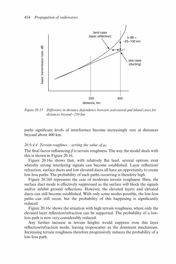
paths significant levels of interference become increasingly rare at distancesbeyond about 400 km.
20.9.4.4 Terrain roughnes – setting the value of μ3
The final factor influencing β is terrain roughness. The way the model deals withthis is shown in Figure 20.16.
Figure 20.16a shows that, with relatively flat land, several options existwhereby strong interfering signals can become established. Layer reflection/refraction, surface ducts and low elevated ducts all have an opportunity to createlow-loss paths. The probability of such paths occurring is therefore high.
Figure 20.16b represents the case of moderate terrain roughness. Here, thesurface duct mode is effectively suppressed as the surface will block the signalsand/or inhibit ground reflections. However, the elevated layers and elevatedducts can still become established. With only some modes possible, the low-losspaths can still occur, but the probability of this happening is significantlyreduced.
Figure 20.16c shows the situation with high terrain roughness, where only theelevated layer reflection/refraction can be supported. The probability of a low-loss path is now very considerably reduced.
Any further increase in terrain heights would suppress even this layerreflection/refraction mode, leaving troposcatter as the dominant mechanism.Increasing terrain roughness therefore progressively reduces the probability of alow-loss path.
Figure 20.15 Difference in distance dependence between sea/coastal and inland cases for
distances beyond ∼250 km
414 Propagation of radiowaves
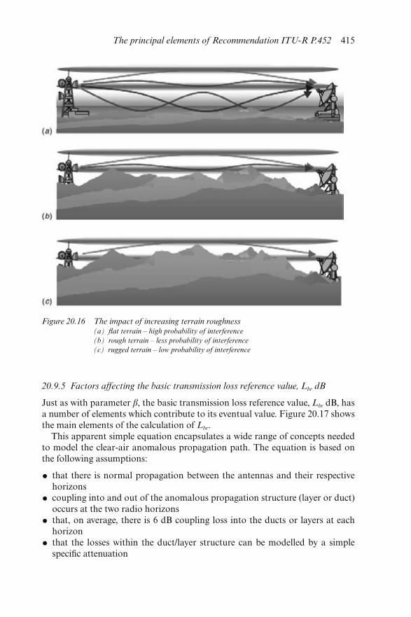
20.9.5 Factors affecting the basic transmission loss reference value, Lbr dB
Just as with parameter β, the basic transmission loss reference value, Lbr dB, hasa number of elements which contribute to its eventual value. Figure 20.17 showsthe main elements of the calculation of Lbr.
This apparent simple equation encapsulates a wide range of concepts neededto model the clear-air anomalous propagation path. The equation is based onthe following assumptions:
• that there is normal propagation between the antennas and their respectivehorizons
• coupling into and out of the anomalous propagation structure (layer or duct)occurs at the two radio horizons
• that, on average, there is 6 dB coupling loss into the ducts or layers at eachhorizon
• that the losses within the duct/layer structure can be modelled by a simplespecific attenuation
Figure 20.16 The impact of increasing terrain roughness(a) flat terrain – high probability of interference
(b) rough terrain – less probability of interference
(c) rugged terrain – low probability of interference
The principal elements of Recommendation ITU-R P.452 415
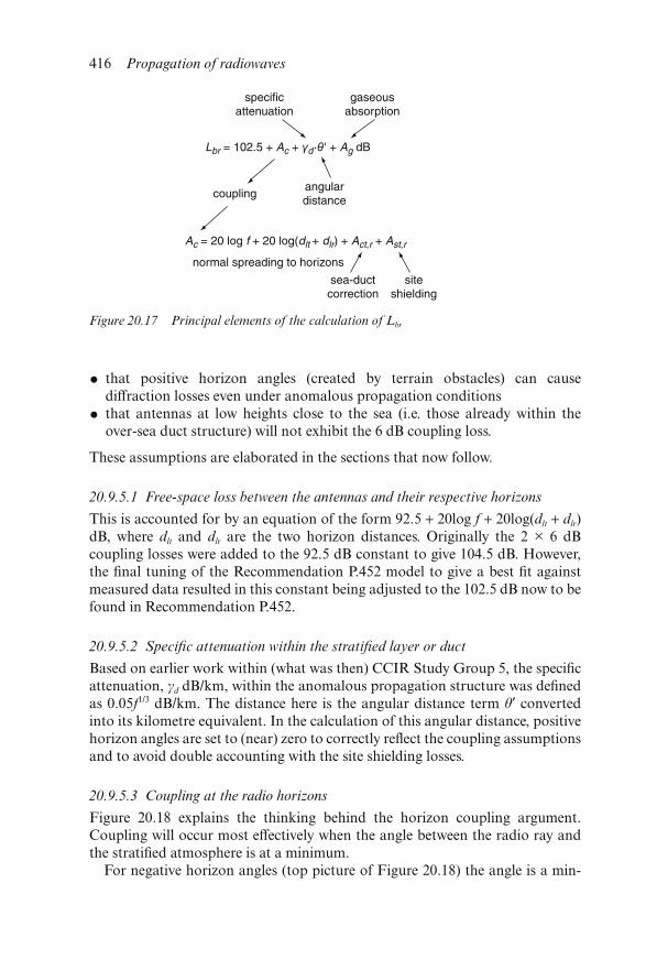
• that positive horizon angles (created by terrain obstacles) can causediffraction losses even under anomalous propagation conditions
• that antennas at low heights close to the sea (i.e. those already within theover-sea duct structure) will not exhibit the 6 dB coupling loss.
These assumptions are elaborated in the sections that now follow.
20.9.5.1 Free-space loss between the antennas and their respective horizons
This is accounted for by an equation of the form 92.5 + 20log f + 20log(dlt + dlr)dB, where dlt and dlr are the two horizon distances. Originally the 2 × 6 dBcoupling losses were added to the 92.5 dB constant to give 104.5 dB. However,the final tuning of the Recommendation P.452 model to give a best fit againstmeasured data resulted in this constant being adjusted to the 102.5 dB now to befound in Recommendation P.452.
20.9.5.2 Specific attenuation within the stratified layer or duct
Based on earlier work within (what was then) CCIR Study Group 5, the specificattenuation, γd dB/km, within the anomalous propagation structure was definedas 0.05f1/3 dB/km. The distance here is the angular distance term θ′ convertedinto its kilometre equivalent. In the calculation of this angular distance, positivehorizon angles are set to (near) zero to correctly reflect the coupling assumptionsand to avoid double accounting with the site shielding losses.
20.9.5.3 Coupling at the radio horizons
Figure 20.18 explains the thinking behind the horizon coupling argument.Coupling will occur most effectively when the angle between the radio ray andthe stratified atmosphere is at a minimum.
For negative horizon angles (top picture of Figure 20.18) the angle is a min-
Figure 20.17 Principal elements of the calculation of Lbr
416 Propagation of radiowaves
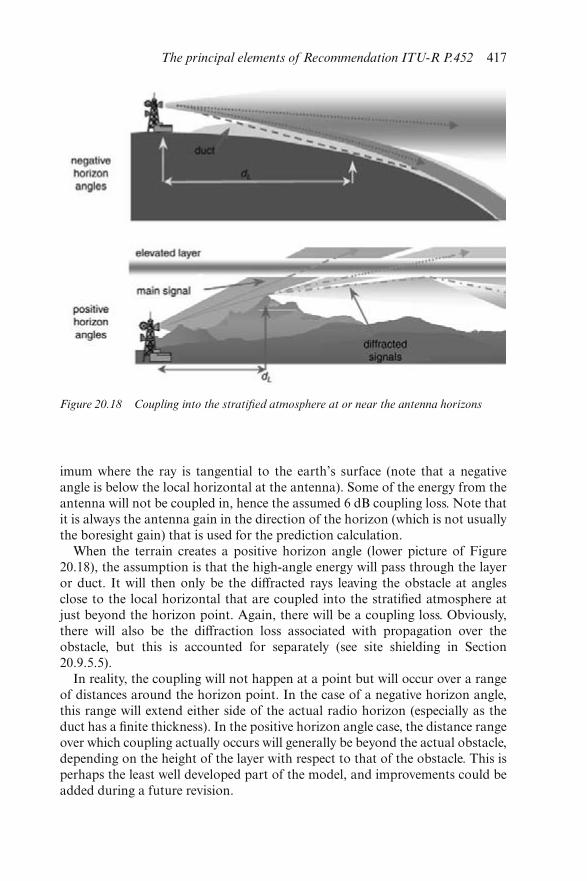
imum where the ray is tangential to the earth’s surface (note that a negativeangle is below the local horizontal at the antenna). Some of the energy from theantenna will not be coupled in, hence the assumed 6 dB coupling loss. Note thatit is always the antenna gain in the direction of the horizon (which is not usuallythe boresight gain) that is used for the prediction calculation.
When the terrain creates a positive horizon angle (lower picture of Figure20.18), the assumption is that the high-angle energy will pass through the layeror duct. It will then only be the diffracted rays leaving the obstacle at anglesclose to the local horizontal that are coupled into the stratified atmosphere atjust beyond the horizon point. Again, there will be a coupling loss. Obviously,there will also be the diffraction loss associated with propagation over theobstacle, but this is accounted for separately (see site shielding in Section20.9.5.5).
In reality, the coupling will not happen at a point but will occur over a rangeof distances around the horizon point. In the case of a negative horizon angle,this range will extend either side of the actual radio horizon (especially as theduct has a finite thickness). In the positive horizon angle case, the distance rangeover which coupling actually occurs will generally be beyond the actual obstacle,depending on the height of the layer with respect to that of the obstacle. This isperhaps the least well developed part of the model, and improvements could beadded during a future revision.
Figure 20.18 Coupling into the stratified atmosphere at or near the antenna horizons
The principal elements of Recommendation ITU-R P.452 417
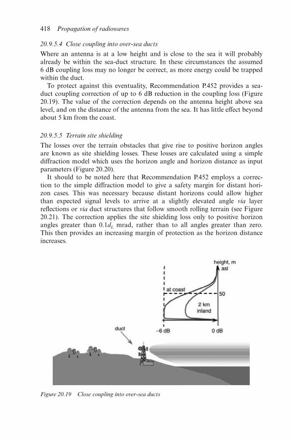
20.9.5.4 Close coupling into over-sea ducts
Where an antenna is at a low height and is close to the sea it will probablyalready be within the sea-duct structure. In these circumstances the assumed6 dB coupling loss may no longer be correct, as more energy could be trappedwithin the duct.
To protect against this eventuality, Recommendation P.452 provides a sea-duct coupling correction of up to 6 dB reduction in the coupling loss (Figure20.19). The value of the correction depends on the antenna height above sealevel, and on the distance of the antenna from the sea. It has little effect beyondabout 5 km from the coast.
20.9.5.5 Terrain site shielding
The losses over the terrain obstacles that give rise to positive horizon anglesare known as site shielding losses. These losses are calculated using a simplediffraction model which uses the horizon angle and horizon distance as inputparameters (Figure 20.20).
It should to be noted here that Recommendation P.452 employs a correc-tion to the simple diffraction model to give a safety margin for distant hori-zon cases. This was necessary because distant horizons could allow higherthan expected signal levels to arrive at a slightly elevated angle via layerreflections or via duct structures that follow smooth rolling terrain (see Figure20.21). The correction applies the site shielding loss only to positive horizonangles greater than 0.1dL mrad, rather than to all angles greater than zero.This then provides an increasing margin of protection as the horizon distanceincreases.
Figure 20.19 Close coupling into over-sea ducts
418 Propagation of radiowaves
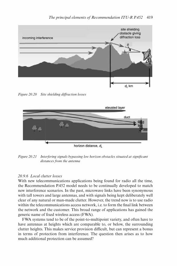
20.9.6 Local clutter losses
With new telecommunications applications being found for radio all the time,the Recommendation P.452 model needs to be continually developed to matchnew interference scenarios. In the past, microwave links have been synonymouswith tall towers and large antennas, and with signals being kept deliberately wellclear of any natural or man-made clutter. However, the trend now is to use radiowithin the telecommunications access network, i.e. to form the final link betweenthe network and the customer. This broad range of applications has gained thegeneric name of fixed wireless access (FWA).
FWA systems tend to be of the point-to-multipoint variety, and often have tohave antennas at heights which are comparable to, or below, the surroundingclutter heights. This makes service provision difficult, but can represent a bonusin terms of protection from interference. The question then arises as to howmuch additional protection can be assumed?
Figure 20.20 Site shielding diffraction losses
Figure 20.21 Interfering signals bypassing low horizon obstacles situated at significant
distances from the antenna
The principal elements of Recommendation ITU-R P.452 419
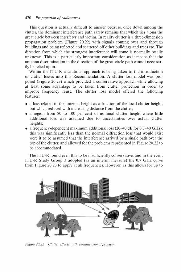
This question is actually difficult to answer because, once down among theclutter, the dominant interference path rarely remains that which lies along thegreat circle between interferer and victim. In reality clutter is a three-dimensionpropagation problem (Figure 20.22) with signals coming over and throughbuildings and being reflected and scattered off other buildings and trees etc. Thedirection from which the strongest interference will come is normally totallyunknown. This is a particularly important consideration as it means that theantenna discrimination in the direction of the great-circle path cannot necessar-ily be relied upon.
Within the ITU-R a cautious approach is being taken to the introductionof clutter losses into this Recommendation. A clutter loss model was pro-posed (Figure 20.23) which provided a conservative approach while allowingat least some advantage to be taken from clutter protection in order toimprove frequency reuse. The clutter loss model offered the followingfeatures:
• a loss related to the antenna height as a fraction of the local clutter height,but which reduced with increasing distance from the clutter;
• a region from 80 to 100 per cent of nominal clutter height where littleadditional loss was assumed due to uncertainties over actual clutterheights;
• a frequency-dependent maximum additional loss (20–40 dB for 0.7–40 GHz);this was significantly less than the normal diffraction loss that would existwere it to be assumed that the interference arrived by a single path over thetop of the clutter, and allowed for the problems represented in Figure 20.22 tobe accommodated.
The ITU-R found even this to be insufficiently conservative, and in the eventITU-R Study Group 3 adopted (as an interim measure) the 0.7 GHz curvefrom Figure 20.23 to apply at all frequencies. However, as this allows for up to
Figure 20.22 Clutter effects: a three-dimensional problem
420 Propagation of radiowaves
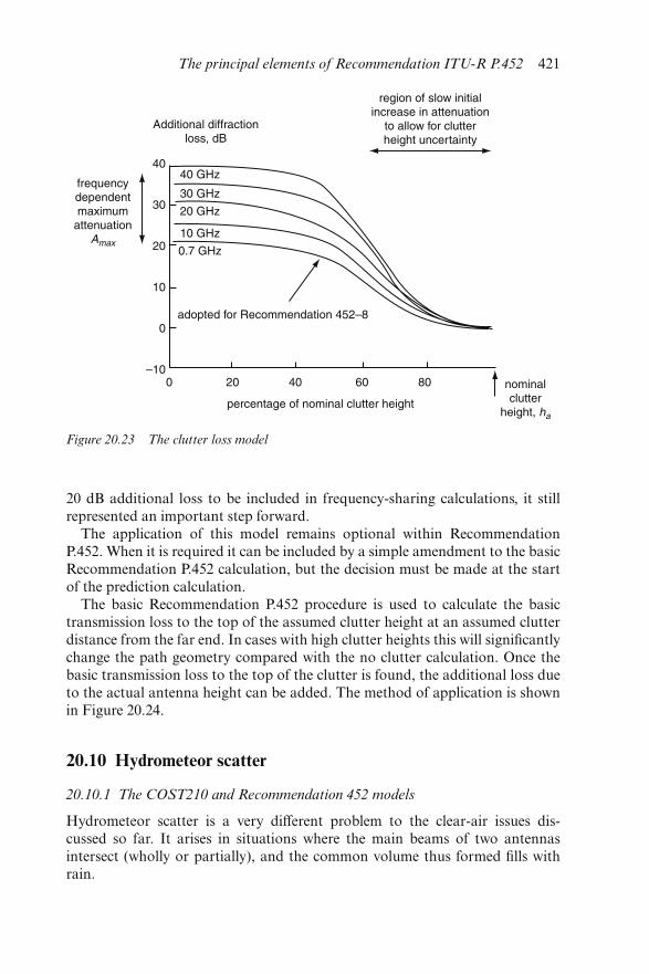
20 dB additional loss to be included in frequency-sharing calculations, it stillrepresented an important step forward.
The application of this model remains optional within RecommendationP.452. When it is required it can be included by a simple amendment to the basicRecommendation P.452 calculation, but the decision must be made at the startof the prediction calculation.
The basic Recommendation P.452 procedure is used to calculate the basictransmission loss to the top of the assumed clutter height at an assumed clutterdistance from the far end. In cases with high clutter heights this will significantlychange the path geometry compared with the no clutter calculation. Once thebasic transmission loss to the top of the clutter is found, the additional loss dueto the actual antenna height can be added. The method of application is shownin Figure 20.24.
20.10 Hydrometeor scatter
20.10.1 The COST210 and Recommendation 452 models
Hydrometeor scatter is a very different problem to the clear-air issues dis-cussed so far. It arises in situations where the main beams of two antennasintersect (wholly or partially), and the common volume thus formed fills withrain.
Figure 20.23 The clutter loss model
The principal elements of Recommendation ITU-R P.452 421
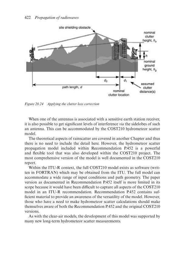
When one of the antennas is associated with a sensitive earth station receiver,it is also possible to get significant levels of interference via the sidelobes of suchan antenna. This can be accommodated by the COST210 hydrometeor scattermodel.
The theoretical aspects of rainscatter are covered in another Chapter and thusthere is no need to include the detail here. However, the hydrometeor scatterpropagation model included within Recommendation P.452 is a powerfuland flexible tool that was also developed within the COST210 project. Themost comprehensive version of the model is well documented in the COST210report.
Within the ITU-R context, the full COST210 model exists as software (writ-ten in FORTRAN) which may be obtained from the ITU. The full model canaccommodate a wide range of input conditions and path geometry. The paperversion as documented in Recommendation P.452 itself is more limited in itsscope because it would have been difficult to capture all aspects of the COST210model in an ITU-R recommendation. Recommendation P.452 contains suf-ficient material to provide an awareness of the versatility of the model. However,those who have a need to make hydrometeor scatter calculations should makethemselves aware of both the Recommendation P.452 and the original COST210versions.
As with the clear-air models, the development of this model was supported bymany new long-term hydrometeor scatter measurements.
Figure 20.24 Applying the clutter loss correction
422 Propagation of radiowaves
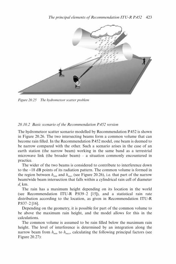
20.10.2 Basic scenario of the Recommendation P.452 version
The hydrometeor scatter scenario modelled by Recommendation P.452 is shownin Figure 20.26. The two intersecting beams form a common volume that canbecome rain filled. In the Recommendation P.452 model, one beam is deemed tobe narrow compared with the other. Such a scenario arises in the case of anearth station (the narrow beam) working in the same band as a terrestrialmicrowave link (the broader beam) – a situation commonly encountered inpractice.
The wider of the two beams is considered to contribute to interference downto the −18 dB points of its radiation pattern. The common volume is formed inthe region between hmin and hmax (see Figure 20.26), i.e. that part of the narrowbeam/wide beam intersection that falls within a cylindrical rain cell of diameterds km.
The rain has a maximum height depending on its location in the world(see Recommendation ITU-R P.839–2 [15]), and a statistical rain ratedistribution according to the location, as given in Recommendation ITU-RP.837–2 [16].
Depending on the geometry, it is possible for part of the common volume tobe above the maximum rain height, and the model allows for this in thecalculations.
The common volume is assumed to be rain filled below the maximum rainheight. The level of interference is determined by an integration along thenarrow beam from hmin to hmax, calculating the following principal factors (seeFigure 20.27):
Figure 20.25 The hydrometeor scatter problem
The principal elements of Recommendation ITU-R P.452 423
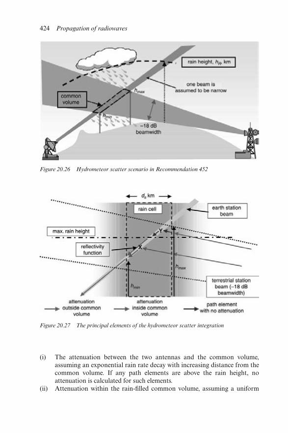
(i) The attenuation between the two antennas and the common volume,assuming an exponential rain rate decay with increasing distance from thecommon volume. If any path elements are above the rain height, noattenuation is calculated for such elements.
(ii) Attenuation within the rain-filled common volume, assuming a uniform
Figure 20.26 Hydrometeor scatter scenario in Recommendation 452
Figure 20.27 The principal elements of the hydrometeor scatter integration
424 Propagation of radiowaves
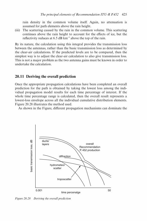
rain density in the common volume itself. Again, no attenuation isassumed for path elements above the rain height.
(iii) The scattering caused by the rain in the common volume. This scatteringcontinues above the rain height to account for the effects of ice, but thereflectivity reduces at 6.5 dB km−1 above the top of the rain.
By its nature, the calculation using this integral provides the transmission lossbetween the antennas, rather than the basic transmission loss as determined bythe clear-air calculations. If the predicted levels are to be compared, then thesimplest way is to adjust the clear-air calculation to also give transmission loss.This is not a major problem as the two antenna gains must be known in order toundertake the calculation.
20.11 Deriving the overall prediction
Once the appropriate propagation calculations have been completed an overallprediction for the path is obtained by taking the lowest loss among the indi-vidual propagation model results for each time percentage of interest. If thewhole time percentage range is calculated, then the overall result represents alowest-loss envelope across all the individual cumulative distribution elements.Figure 20.28 illustrates the method used.
As shown in the Figure, different propagation mechanisms can dominate the
Figure 20.28 Deriving the overall prediction
The principal elements of Recommendation ITU-R P.452 425
prediction over different parts of the time percentage range, depending on thespecific input conditions for the calculations. This can, and does, happen onpractical paths, once again illustrating the complexity of the problem that therecommendation sets out to solve.
Recommendation ITU-R P.452 has now been used for many millions of pathcalculations associated with the planning of new systems and the protection ofwhat exists already. Although there is always a need to refine and improve suchtools as the requirements grow more complex, the version which currently exists(Recommendation P.452–9) provides a reliable and flexible general purpose toolfor interference analysis.
20.12 References
1 COST210 Management Committee: ‘Influence of the atmosphere oninterference between radio communication systems at frequencies above1 GHz’. Final report of COST Project 210, Commission of the EuropeanCommunities, Luxembourg, April 1991
2 Recommendation ITU-R P.452-9: ‘Prediction procedure for the evaluationof microwave interference between stations on the surface of the earth atfrequencies above about 0.7 GHz’, 1999
3 BYE, G.D.: ‘Radio-meteorological aspects of anomalous propagation inNW Europe”, BT Technical Journal; 1988, 6, 3
4 HEWITT, M.T. et al.: ‘Worst month prediction model for transhorizonmicrowave interference’, Electron. Lett., 1989, 25, (24) pp.167
5 BEAN, B. et al.: ‘A world atlas of atmospheric radio refractivity’, ESSAmonograph 1, US Dept. of Commerce, Institute for TelecommunicationsSciences, Boulder, Colorado, 1966
6 Recommendation ITU-R P.676-4, ‘Attenuation by atmospheric gases’,1999
7 Recommendation ITU-R P.526-6 ‘Propagation by diffraction’, 19998 HEWITT, M.T. and MEHLER, M.J.: ‘A versatile diffraction modelling
techniques for microwave interference propagation prediction’, Inter-national Wroclaw Symposium on Electromagnetic compatibility, Wroclaw,Poland, 1992
9 SHARPLES, P.A. and MEHLER, M.J.: ‘A cascaded cylinder model forpredicting terrain diffraction loss at microwave frequencies’, Proc. IEE1989, 136, pp.331–337
10 EPSTEIN, J. and PETERSON, D.W.: ‘An experimental study of wavepropagation at 850 Mc’, Proc IRE, 1953, 41, pp.595–611
11 Recommendation ITU-R P.526-3: ‘Propagation by diffraction’, 199212 DEYGOUT, J.: ‘Multiple knife-edge diffraction of microwaves’, IEEE
Trans. Antennas Prop., 14, pp.480–48913 RICE, P.L. et. al.: ‘Transmission loss predictions for tropospheric com-
munication circuits’. NBS technical note 101, revised January 1967, USNational Bureau of Standards, vol. II
14 YEH, L.P.: ‘Simple methods of designating troposcatter circuits’, IRETrans. Comms. Sys., CS-8 (III), p.119
426 Propagation of radiowaves
15 Recommendation ITU-R P.839-2: ‘Rain height model for predictionmethods’, 1999
16 Recommendation ITU-R P.837-2, ‘Characteristics of precipitation forpropagation modelling’, 1999
The principal elements of Recommendation ITU-R P.452 427

Chapter 21
Earth–space propagation: RecommendationITU-R P.618
R.G. Howell
21.1 Introduction
Recommendation ITU-R P.618 [1] presents propagation data and step-by-stepmethods for predicting the performance of earth–space radio systems operatingin frequency bands between about 1 GHz and 55 GHz and applicable to averageannual percentage times in the range 0.001 per cent to 50 per cent. This recom-mendation deals only with effects relating to the wanted signal. Interferenceaspects are covered in Recommendations ITU-R P.452 [2], P.619 [3] and P.1412 [4].
There is insufficient space within this Chapter to present all the details of theprediction methods given in Recommendation ITU-R P.618 and, therefore, abroad description will be given together with references to related ITUdocuments.
21.2 Overview
21.2.1 General
The propagation effects relevant to the design of earth–space radio systems aresomewhat different from those applicable to terrestrial line-of-sight radio links.In particular, multipath propagation produced by atmospheric layers can beneglected except for paths at low elevation angles (<4°). However, the effects ofthe ionosphere (at frequencies below about 4 GHz), high altitude ice particlesand short-term variations in atmospheric radio refractive index, producing rapidamplitude and phase variations in the signal (mainly at elevation angles below5°), must be taken into account. Also, during fine weather conditions, the radionoise emission from objects within the main beam of the earth-station antenna
is usually significantly less than that for terrestrial line-of-sight antennas. Thisallows low-noise receiving systems to be used, however, the effects of radio noisefrom the cosmos, the atmosphere and the environment of the antenna must thenbe taken into account.
The effects of rain are similar to those on terrestrial line-of-sight links withthe exception that, in the case of earth–space links, the effective path lengththrough the rain is determined by the maximum height of the rain and itsvertical and horizontal distribution, rather than the length of the link and thehorizontal distribution of the rain along the path (the situation with terrestrialline-of-sight links).
21.2.2 Propagation effects
The main propagation effects that must be considered in the design of earth–space radio systems are:
• free-space loss
• ionospheric effects: Faraday rotation of the plane of polarisation, dispersion,excess time delay and ionospheric scintillation
• absorption by atmospheric gases
• absorption, scattering and depolarisation by hydrometeors (water dropletsand ice particles of various forms in precipitation, clouds etc.)
• radio noise emissions from the cosmos, sun, moon and absorbing mediawithin the atmosphere
• loss of signal due to divergence of the earth-station antenna beam resultingfrom the normal radio refractive index structure of the atmosphere
• a decrease in the effective antenna gain, due to phase decorrelation acrossthe antenna aperture, caused by irregularities in the radio refractive indexstructure of the atmosphere
• slow fading due to beam bending caused by large-scale changes in the radiorefractive index of the atmosphere
• more rapid fading (scintillation) and variations in angle of arrival, due tosmall-scale variations in the radio refractive index of the atmosphere
• possible limitations in bandwidth due to multiple scattering or multipatheffects, especially in high-capacity digital systems
• attenuation by the local environment of the earth-station antenna (buildings,trees etc.)
• short-term variations in the ratio of the attenuations at the uplink anddownlink frequencies, which may affect the accuracy of adaptive fadecountermeasures e.g. transmitter power control
• for nongeostationary satellite (nonGSO) systems, the effect of the varyingsatellite elevation angle.
At elevation angles greater than 10° only gaseous attenuation, rain andcloud attenuation and possibly (to a lesser extent) scintillation will contributesignificantly to the total atmospheric loss.
430 Propagation of radiowaves
21.3 Ionospheric effects
The effect of the ionosphere on signals transmitted over earth–space paths maybe important, particularly at frequencies below 4 GHz, but rapidly becomeless important as the frequency approaches and exceeds 10 GHz, see alsoChapter 17. The effects include:
• Faraday rotation: a linearly polarised wave propagating through theionosphere undergoes a progressive rotation of the plane of polarisation;
• dispersion, which results in a differential time delay across the bandwidth ofthe transmitted signal;
• excess time delay relative to the delay a signal would have if it traversed thesame path with no ionosphere;
• ionospheric scintillation: inhomogeneities of electron density in the iono-sphere cause refractive focusing or defocusing of radiowaves and lead toamplitude fluctuations termed scintillation; ionospheric scintillation is maxi-mum near the geomagnetic equator and smallest in the mid-latitude regions,the auroral zones are also regions of large ionospheric scintillation; strongscintillation is Rayleigh distributed in amplitude, weaker scintillation is nearlylog-normally distributed; these fluctuations decrease with increasing fre-quency and depend upon path geometry, location, season, solar activity andlocal time;
• phase fluctuations having a spectral density proportional to 1/f 3, where f isthe Fourier frequency of the fluctuation, accompany the amplitudefluctuations.
Table 21.1 shows the frequency dependence and order of magnitude of some ofthe ionospheric effects for frequencies between 1 GHz and 10 GHz [1]. In termsof telecommunications systems the effect of the ionosphere can be ignored atfrequencies above about 10 GHz.
Further details on the effects of the ionosphere can be found in Recommenda-tion ITU-R P.531 [5].
21.4 Clear-air effects
21.4.1 General
Other than atmospheric absorption, clear-air effects in the absence of precipita-tion are unlikely to produce serious fading in space telecommunication systemsoperating at frequencies below about 10 GHz and at elevation angles above 10°.However, at low elevation angles (≤10°) and at frequencies above about 10 GHztropospheric scintillation can, on occasion, cause serious degradations inperformance. At very low elevation angles (≤4° on inland paths, and ≤5° onover-water or coastal paths), fading due to multipath propagation effects can beparticularly severe.
Earth–space propagation: Recommendation ITU-R P.618 431
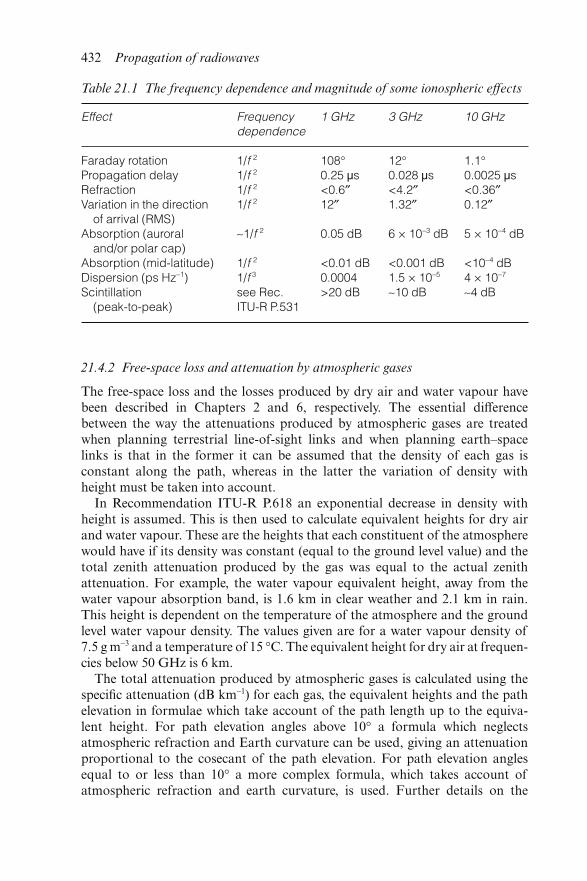
21.4.2 Free-space loss and attenuation by atmospheric gases
The free-space loss and the losses produced by dry air and water vapour havebeen described in Chapters 2 and 6, respectively. The essential differencebetween the way the attenuations produced by atmospheric gases are treatedwhen planning terrestrial line-of-sight links and when planning earth–spacelinks is that in the former it can be assumed that the density of each gas isconstant along the path, whereas in the latter the variation of density withheight must be taken into account.
In Recommendation ITU-R P.618 an exponential decrease in density withheight is assumed. This is then used to calculate equivalent heights for dry airand water vapour. These are the heights that each constituent of the atmospherewould have if its density was constant (equal to the ground level value) and thetotal zenith attenuation produced by the gas was equal to the actual zenithattenuation. For example, the water vapour equivalent height, away from thewater vapour absorption band, is 1.6 km in clear weather and 2.1 km in rain.This height is dependent on the temperature of the atmosphere and the groundlevel water vapour density. The values given are for a water vapour density of7.5 g m−3 and a temperature of 15 °C. The equivalent height for dry air at frequen-cies below 50 GHz is 6 km.
The total attenuation produced by atmospheric gases is calculated using thespecific attenuation (dB km−1) for each gas, the equivalent heights and the pathelevation in formulae which take account of the path length up to the equiva-lent height. For path elevation angles above 10° a formula which neglectsatmospheric refraction and Earth curvature can be used, giving an attenuationproportional to the cosecant of the path elevation. For path elevation anglesequal to or less than 10° a more complex formula, which takes account ofatmospheric refraction and earth curvature, is used. Further details on the
Table 21.1 The frequency dependence and magnitude of some ionospheric effects
Effect Frequencydependence
1 GHz 3 GHz 10 GHz
Faraday rotation 1/f 2 108° 12° 1.1°Propagation delay 1/f 2 0.25 �s 0.028 �s 0.0025 �sRefraction 1/f 2 <0.6″ <4.2″ <0.36″Variation in the direction
of arrival (RMS)1/f 2 12″ 1.32″ 0.12″
Absorption (auroraland/or polar cap)
∼1/f 2 0.05 dB 6 × 10⁻³ dB 5 × 10⁻⁴ dB
Absorption (mid-latitude) 1/f 2 <0.01 dB <0.001 dB <10−4 dBDispersion (ps Hz−1) 1/f 3 0.0004 1.5 × 10⁻⁵ 4 × 10⁻⁷
Scintillation(peak-to-peak)
see Rec.ITU-R P.531
>20 dB ∼10 dB ∼4 dB
432 Propagation of radiowaves
losses produced by dry air and water vapour can be found in RecommendationITU-R P.676 [6].
21.4.3 Phase decorrelation across the antenna aperture
Incoherence of the wave front of a wave incident on a receiving antenna iscaused by small-scale irregularities in the refractive index structure of theatmosphere. This results in an antenna-to-medium coupling loss that can bedescribed as a decrease of the antenna gain. The loss increases both withincreasing frequency and decreasing elevation angle, and is a function ofantenna diameter. Although not explicitly accounted for in the atmosphericrefraction models discussed below, this effect is negligible in comparison.
21.4.4 Beam spreading loss
The amount of downward ray bending produced by the regular decrease of theradio refractive index of the atmosphere with height under average refractivityconditions is a function of the elevation angle of the ray, and increases as theelevation angle of the ray is reduced (particularly for elevations below about 3°).Hence, rays at the top and bottom of the antenna main beam travel along pathshaving slightly different elevation angles and the resulting differential ray bend-ing (top to bottom) produces an additional divergence of the beam in the verti-cal plane. Therefore, the cross-sectional area of the beam is increased and thegain of the antenna is reduced. It should be noted that there is no increase in thedivergence of the beam in the horizontal plane. The loss in the antenna gainresulting from this beam spreading is independent of frequency, over the rangeof 1–100 GHz (see Recommendation ITU-R P.834 [7] for further details).
The loss Abs due to beam spreading in regular refractive conditions can beignored at elevation angles above about 3° at latitudes less than 53° and aboveabout 6° at higher latitudes.
At all latitudes, the beam spreading loss in the average year at elevation anglesless than 5° can be estimated from:
Abs = 2.27 – 1.16 log(1 + θ0) dB for Abs > 0 (21.1)
where θ0 is the apparent elevation angle (mrad), taking into account the effectsof refraction.
Recommendation ITU-R P.618 also gives formulae (which are dependent onthe latitude of the earth station) for calculating the loss produced by beamspreading for the average worst month.
21.4.5 Scintillation and multipath fading
The magnitude of tropospheric scintillation depends on the magnitude andstructure of the refractive index variations, increasing with frequency and withthe path length through the medium, and decreasing as the antenna beamwidth
Earth–space propagation: Recommendation ITU-R P.618 433
decreases because of aperture averaging. Monthly-averaged RMS fluctuationsare well correlated with the wet term of the radio refractivity, Nwet, whichdepends on the water vapour content of the atmosphere. Nwet may be estimatedfor periods of a month or longer from meteorological data obtained at thesurface.
At very small percentages of time, or conversely large fade depths (greaterthan about 10 dB), the fading at very low elevation angles (≤4° on inland paths,and ≤5° on over-water or coastal paths) is observed to be more severe than thatpredicted due to scintillation. The fading is also observed to have a charactersimilar to multipath fading on terrestrial links. Like the distribution on terres-trial links, the distribution for very-low-angle satellite links also appears corre-lated with refractivity gradient statistics. The overall fading distribution shows agradual transition from a scintillation distribution at large exceedance percent-ages to a multipath fading distribution (with a slope of 10 dB decade−1) at smallpercentages.
Recommendation ITU-R P.618 gives a general method for predicting thecumulative distribution of tropospheric scintillation at elevation angles ofgreater than 4°. The method is based on monthly or longer averages of surfaceambient temperature (t) and relative humidity (H) for the site. As the averages oft and H vary with season, distributions of scintillation fade depth exhibit sea-sonal variations, which may also be predicted by using seasonal averages oft and H in the method. The procedure has been tested at frequencies between7 and 14 GHz, but is recommended for applications up to at least 20 GHz.
Recommendation ITU-R P.618 also gives methods for calculating both thedeep fading (> 25 dB) and the shallow fading part of the scintillation/multipathfading distribution for paths having elevation angles of less than 5°. Themethods estimate the average worst month and average year fading distribu-tions, taking account of the combined effects of beam spreading, scintillationand multipath fading.
The net fade distribution due to tropospheric refractive effects is the combin-ation of the beam spreading, scintillation and multipath fading effects describedabove. Tropospheric and ionospheric scintillation distributions may be com-bined by summing the respective time percentages for which specified fade levelsare exceeded.
21.4.6 Angle of arrival
Because of the downward bending of the wave produced by the normal decreasein radio refractive index with increasing height an earth-station antenna must bepointed at an elevation angle slightly greater than that which would apply in theabsence of refraction. For example, the total angular refraction (the increase inapparent elevation) is about 0.65°, 0.35° and 0.25°, for path elevation angles of1°, 3° and 5°, respectively, for a tropical maritime atmosphere. For a polarcontinental climate the corresponding values are 0.44°, 0.25° and 0.17°. Otherclimates will have values between these two extremes. The day-to-day variation
434 Propagation of radiowaves
in apparent elevation is of the order of 0.1° (RMS) at 1° elevation, but thevariation decreases rapidly with increasing elevation angle.
Short-term variations, due to changes in the refractivity-height variation, maybe of the order of 0.02° (RMS) at 1° elevation, again decreasing rapidly withincreasing elevation angle. In practice, it is difficult to distinguish between theeffect of the short-term changes in the refractivity-height distribution and theeffect of random irregularities superimposed on that distribution. A statisticalanalysis of the short-term angle-of-arrival fluctuation at 19.5 GHz and at anelevation angle of 48° suggests that both in elevation and azimuth directions,standard deviations of angle-of-arrival fluctuations are about 0.002° at thecumulative time percentage of one per cent. The seasonal variation of angle-of-arrival fluctuations suggests that the fluctuations increase in summer anddecrease in winter. The diurnal variation suggests that they increase in thedaytime and decrease both in the early morning and the evening.
Further information on elevation-angle errors due to refraction may be foundin Recommendation ITU-R P.834 [7].
21.4.7 Propagation delays
Recommendation ITU-R P.834 [7] provides data on radio meteorologically-based methods for estimating the mean value and the variability in the propaga-tion delay (or range error) produced by the troposphere for earth–space paths.At frequencies above 10 GHz, the delay produced by the ionosphere is generallysmaller than that for the troposphere, but may have to be considered in specialcases. Further information on the delay produced by the ionosphere can befound in Recommendation ITU-R P.531 [5].
Range determination to centimetre accuracy requires careful consideration ofthe various contributions to excess range delay. A dry atmosphere adds a delayequivalent to an additional 2.3 m to a zenith path. However, the largest sourceof uncertainty in the path length is produced by the water vapour component ofthe atmosphere, due to the variability of the water vapour concentration. Forexample, this produces a delay equivalent to an additional path length of 10 cmfor a zenith path and a reference atmosphere with a surface water vapourconcentration of 7.5 g m−3 and 2 km scale height (see Recommendation ITU-RP.676 [6]).
For current satellite telecommunication applications, additional propagationdelays contributed by precipitation are sufficiently small to be ignored.
21.5 Hydrometeor effects
21.5.1 General
The physical basis for the absorption, scattering and depolarisation by hydro-meteors has been discussed in Chapter 12. It was shown in this Chapter that the
Earth–space propagation: Recommendation ITU-R P.618 435
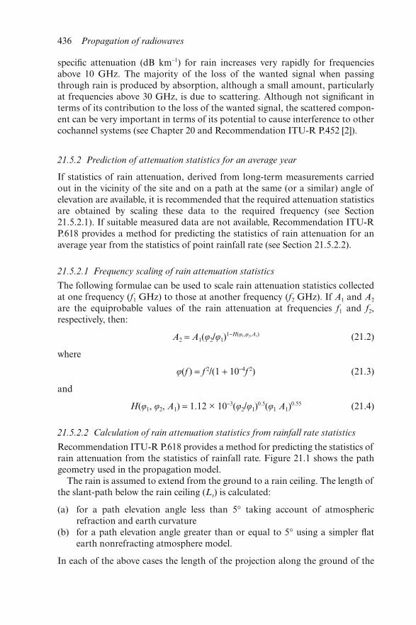
specific attenuation (dB km−1) for rain increases very rapidly for frequenciesabove 10 GHz. The majority of the loss of the wanted signal when passingthrough rain is produced by absorption, although a small amount, particularlyat frequencies above 30 GHz, is due to scattering. Although not significant interms of its contribution to the loss of the wanted signal, the scattered compon-ent can be very important in terms of its potential to cause interference to othercochannel systems (see Chapter 20 and Recommendation ITU-R P.452 [2]).
21.5.2 Prediction of attenuation statistics for an average year
If statistics of rain attenuation, derived from long-term measurements carriedout in the vicinity of the site and on a path at the same (or a similar) angle ofelevation are available, it is recommended that the required attenuation statisticsare obtained by scaling these data to the required frequency (see Section21.5.2.1). If suitable measured data are not available, Recommendation ITU-RP.618 provides a method for predicting the statistics of rain attenuation for anaverage year from the statistics of point rainfall rate (see Section 21.5.2.2).
21.5.2.1 Frequency scaling of rain attenuation statistics
The following formulae can be used to scale rain attenuation statistics collectedat one frequency (f1 GHz) to those at another frequency (f2 GHz). If A1 and A2
are the equiprobable values of the rain attenuation at frequencies f1 and f2,respectively, then:
A2 = A1(φ2/φ1)1−H(φ1,φ2,A1) (21.2)
where
φ(f ) = f 2/(1 + 10−4f 2) (21.3)
and
H(φ1, φ2, A1) = 1.12 × 10⁻³(φ2/φ1)0.5(φ1 A1)
0.55 (21.4)
21.5.2.2 Calculation of rain attenuation statistics from rainfall rate statistics
Recommendation ITU-R P.618 provides a method for predicting the statistics ofrain attenuation from the statistics of rainfall rate. Figure 21.1 shows the pathgeometry used in the propagation model.
The rain is assumed to extend from the ground to a rain ceiling. The length ofthe slant-path below the rain ceiling (Ls) is calculated:
(a) for a path elevation angle less than 5° taking account of atmosphericrefraction and earth curvature
(b) for a path elevation angle greater than or equal to 5° using a simpler flatearth nonrefracting atmosphere model.
In each of the above cases the length of the projection along the ground of the
436 Propagation of radiowaves
slant path (LG) is calculated. This length is then used to determine horizontaland vertical reduction factors, which take account of the spatial nonuniformityof the rain both horizontally and vertically. The rain-specific attenuation, corre-sponding to a rainfall rate equal to that exceeded for 0.01 per cent of an averageyear (R0.01), is then used with the effective path length to calculate the attenu-ation exceeded for 0.01 per cent of an average year. The attenuation exceededfor other percentage times in the range 0.001 per cent to 5 per cent is thenderived from the 0.01 per cent attenuation value.
Clearly, a key meteorological parameter used in this model is the rainfall rateexceeded for 0.01 per cent of an average year (R0.01). Rainfall rate statistics arestrongly dependent on the integration time used in determining the rainfall rates.An integration time of one minute should be used to determine the value of R0.01
used in this model. If a value for R0.01 is not available from long-term locallymeasured data then an estimate can be obtained from maps of rainfall rate givenin Recommendation ITU-R P.837 [8].
21.5.3 Seasonal variations – worst month
It should be noted that the propagation model described in Section 21.5.2.2gives the rain attenuation statistics for an average year. System planning oftenrequires statistics for an average worst month. These can be derived fromthe average annual statistics using methods given in Recommendation ITU-RP.841 [9].
First, the average annual time percentage, p per cent, corresponding to thedesired average worst month time percentage pw per cent is determined using arelationship between the two that takes into account the climatic region. Then
Figure 21.1 Path geometry used in the Recommendation ITU-R P.618 rain attenuation
prediction model
Earth–space propagation: Recommendation ITU-R P.618 437
the attenuation exceeded for pw per cent of the average worst month is equal tothe attenuation exceeded for p per cent of an average year, as determined usingeither the propagation model described in Section 21.5.2.2, or by scaling fromlong-term statistics as described in Section 21.5.2.1.
Curves, giving the variation of worst month values from their mean, areprovided in Recommendation ITU-R P.678 [10].
21.5.4 Year-to-year variability of rain attenuation statistics
Distributions of rain attenuation measured on the same path at the same fre-quency and on the polarisation may show marked year-to-year variations. In therange 0.001 per cent to 0.1 per cent of the year, the attenuation values at a fixedprobability level are observed to vary by more than 20 per cent RMS.
21.5.5 Fade duration and rate of change
The durations of rain fades exceeding a specified attenuation level are approxi-mately log-normally distributed. Median durations are of the order of severalminutes. No significant dependence of these distributions on fade depth is evi-dent in most measurements for fades of less than 20 dB, implying that the largertotal time percentage of fades observed at lower fade levels or at higher frequen-cies is composed of a larger number of individual fades having more or less thesame distribution of durations. Significant departures from a log-normal distri-bution seem to occur for fade durations of less than about half a minute. Fadedurations at a specified fade level tend to increase with decreasing elevationangle.
Data are needed on the contribution of attenuation events shorter than tenseconds to the total fading time for the planning of integrated services digitalnetwork (ISDN) connections via satellite. This information is especially relevantfor the attenuation level corresponding to the outage threshold, where eventslasting longer than ten seconds contribute to system unavailable time, andshorter events affect system performance during available time.
Existing data indicates that, in the majority of cases, the exceedance timeduring available time is 2 per cent to 10 per cent of the net exceedance time.However, at low elevation angles, where the short period signal fluctuations dueto tropospheric scintillation become statistically significant, there are some casesfor which the exceedance time during available time is far larger than in the caseat higher elevation earth–space paths.
The rate of change of attenuation (fading rate) can be an important factorwhen fade mitigation techniques, such as adaptive transmit power control (Sec-tion 21.11.2), are considered. There is broad agreement that the distributions ofpositive and negative fade rates are log-normally distributed and very similar toeach other, however, the dependence of fade rate on fade depth has not beenestablished.
438 Propagation of radiowaves
21.5.6 Short-term variations in the frequency scaling ratio of attenuations
Data on the instantaneous ratio of the rain attenuation at different frequenciesis relevant to the application of a variety of adaptive fade techniques. Thefrequency-scaling ratio has been found to be log-normally distributed, and isinfluenced by rain type and rain temperature. Data reveal that the short-termvariations in the attenuation ratio can be significant, and are expected toincrease with decreasing path elevation angle.
21.6 Estimation of total attenuation produced by multiple sources
For systems operating at frequencies above about 18 GHz, and especially thoseoperating at low elevation angles and/or with small fade margins, the effect ofmultiple sources of simultaneously occurring atmospheric attenuation must beconsidered.
The total attenuation (AT(p) dB) is the result of the combined effect of rain,gases, clouds and scintillation.
Defining:
AR (p): attenuation (dB) due to rain exceeded for a probability p per cent,estimated using Recommendation ITU-R P.618 [1]
AC (p): attenuation (dB) due to clouds exceeded for a probability p per cent,estimated using Recommendation ITU-R P.840 [11]
AG: mean gaseous attenuation (dB) due to water vapour and dry air,estimated using Recommendation ITU-R P.676 [6]
AS (p): attenuation (dB) due to tropospheric scintillation exceeded for a prob-ability p per cent, estimated using Recommendation ITU-R P.618 [1]
where p is the probability of the attenuation being exceeded in the range 50 percent to 0.001 per cent. A general method for calculating total attenuation (AT
(p) ) for a given probability is given by:
AT (p) = AG + √(AR (p) + AC (p) )2 + A2S (p) (21.5)
However, for p < 1 per cent, AC(p) = 0 because cloud attenuation is alreadyincluded in the rain attenuation prediction method used in RecommendationITU-R P.618.
Some simplifications can be made to Eqn. 21.5 under certain conditions aslisted in Table 21.2.
21.7 System noise
The atmospheric contribution to the noise temperature of an earth-stationantenna (and hence to the system noise) increases as the loss produced byabsorption in atmospheric gases and rain along the path increases. For earth
Earth–space propagation: Recommendation ITU-R P.618 439
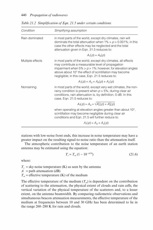
stations with low-noise front ends, this increase in noise temperature may have agreater impact on the resulting signal-to-noise ratio than the attenuation itself.
The atmospheric contribution to the noise temperature of an earth stationantenna may be estimated using the equation:
Ts = Tm (1 − 10−A/10) (21.6)
where:
Ts = sky-noise temperature (K) as seen by the antennaA = path attenuation (dB)Tm = effective temperature (K) of the medium
The effective temperature of the medium (Tm) is dependent on the contributionof scattering to the attenuation, the physical extent of clouds and rain cells, thevertical variation of the physical temperature of the scatterers and, to a lesserextent, on the antenna beamwidth. By comparing radiometric observations andsimultaneous beacon attenuation measurements, the effective temperature of themedium at frequencies between 10 and 30 GHz has been determined to lie inthe range 260–280 K for rain and clouds.
Table 21.2 Simplification of Eqn. 21.5 under certain conditions
Condition Simplifying assumption
Rain dominated in most parts of the world, except dry climates, rain willdominate the total attenuation when 1% > p > 0.001%; in thiscase the other effects may be neglected and the totalattenuation given in Eqn. 21.5 reduces to:
AT(p) = AR(p)
Multiple effects in most parts of the world, except dry climates, all effectsmay contribute a measurable level of propagationimpairment when 5% > p > 1%; however, for elevation anglesabove about 10° the effect of scintillation may becomenegligible; in this case, Eqn. 21.5 reduces to:
AT(p) = AG + AR(p) + AC(p)
Nonraining in most parts of the world, except very wet climates, the non-rainy condition is present when p > 5%; during clear airconditions, rain attenuation is, by definition, 0 dB. In thiscase, Eqn. 21.5 reduces to:
AT(p) = AG + √A2C(p) + A2
S(p)
when operating at elevation angles greater than about 10°,scintillation may become negligible during clear airconditions and Eqn. 21.5 will further reduce to:
AT(p) = AG + AC(p)
440 Propagation of radiowaves
When the attenuation is known, the following effective temperatures of theatmospheric media may be used to obtain an upper limit to the sky-noisetemperature at frequencies below 60 GHz:
Tm = 280 K for clouds (21.7)
Tm = 260 K for rain (21.8)
The sun and, to a lesser extent, the moon can occasionally contribute signifi-cantly to the noise temperature of an earth-station antenna at all frequencies. Inaddition, radio noise from other discrete sources such as Cygnus A and X,Cassiopeia A, Taurus and The Crab nebula could also be important. Radionoise from the cosmic background is only of importance at frequenciesbelow about 2 GHz. For further information on sources of radio noise andmethods for determining the system noise temperature of an earth station seeRecommendation ITU-R P.372 [12].
21.8 Cross-polarisation effects
21.8.1 General
The capacity of space telecommunication systems can be increased by reusingfrequencies on orthogonal polarisations. However, this technique can berestricted by depolarisation of the signal as it passes through the atmosphere. Ofparticular importance is the depolarisation produced by hydrometeors (i.e. rainor ice particles in various forms) in the troposphere and, at frequencies below4 GHz, depolarisation produced by the ionosphere.
Depolarisation by hydrometeors can occur due to:
(a) The nonspherical (oblate) shape of large raindrops. This producesdifferential attenuation and phase shift between components of the incidentwave polarised parallel and perpendicular to the principal axes of theraindrop.
(b) Ice particles, in the form of needles and plates. In this case the depolarisa-tion results from a differential phase shift between components of the inci-dent wave polarised parallel and perpendicular to the principal axes of theice crystals.
The physical basis for both these effects is discussed in some detail in Chapter 12.Depolarisation by the ionosphere results from Faraday rotation of the plane
of polarisation of a linearly polarised wave by the ionosphere. This is discussedin Chapter 16 and also in Recommendation ITU-R P.531 [5]. As much as 1° ofrotation may be encountered at 10 GHz, and greater rotations at lower frequen-cies. As seen from an earth station, the planes of polarisation rotate in the samedirection on the uplinks and downlinks. Therefore, if the same antenna is usedboth for transmitting and receiving it is not possible to compensate for Faradayrotation by rotating the feed system of the antenna.
Earth–space propagation: Recommendation ITU-R P.618 441
21.8.2 Calculation of long-term statistics of hydrometeor-induced cross
polarisation
Recommendation ITU-R P.618 gives a method for predicting the long-term statistics of hydrometeor-induced cross polarisation from the long-termstatistics of rain attenuation.
The following terms are used in the method:
(i) A frequency-dependent term (Cf): this takes account of the frequencydependence of the depolarisation produced by rain.
(ii) A term dependent on the statistics of rain attenuation (CA): this is based onthe observed correlation between the depolarisation and the attenuationproduced by rain.
(iii) An elevation angle dependent term (Cθ): large raindrops can be modelled asoblate (flattened) spheres having their minimum dimension (i.e. the dimen-sion along their axis of symmetry) aligned with a distribution of angles(canting angles) having a mean which is approximately vertical. Hence, theraindrop asymmetry, when viewed along the path, will decrease as the pathelevation increases i.e. the raindrop cross section normal to the path willchange from being approximately elliptical for a low elevation path tobeing approximately circular for a vertical path (an extreme case). Since,the depolarisation of a wave passing through a collection of raindrops isdirectly related to the asymmetry in the cross section normal to the path,waves traversing low-angle paths will suffer more depolarisation than thosetraversing high-angle paths. The elevation angle dependent term (Cθ) takesaccount of this variation.
(iv) A term giving the polarisation improvement factor (Cτ): this takes accountof the polarisation type (linear or circular) and, if applicable, the orienta-tion of the linearly polarised wave relative to the axis of symmetry of theraindrops. In the case of a linearly polarised wave, if τ is the tilt angle ofthe electric field vector with respect to the horizontal, then the improve-ment factor Cτ = 0 for τ = 45° and reaches a maximum value of 15dB forτ = 0° or 90°. For circular polarisation a value of 45° should be used for τ.Thus, a linearly polarised wave suffers the greatest depolarisation when it isaligned at 45° to the horizontal (equal to that for a circularly polarisedwave) and the least depolarisation when it is aligned either vertically orhorizontally.
(v) A raindrop canting angle dependent term (Cσ): This takes account of thespread in the raindrop canting angles around the distribution mean value.The effective standard deviation of the raindrop canting angle distributionexpressed in degrees (σ) has a value of about 0°, 5°, 10° and 15° for 1 percent, 0.1 per cent, 0.01 per cent and 0.001 per cent of the time, respectively.
First, the XPD (not exceeded for p per cent of the time) associated with thedepolarisation produced by rain (XPDrain) is calculated using:
XPDrain = Cf − CA + Cτ + Cθ + Cσ (21.9)
442 Propagation of radiowaves
Then, based on the observed correlation between rain and ice depolarisation,the XPD (not exceeded for p per cent of the time) associated with the depolarisa-tion produced by ice crystals (Cice) is calculated from XPDrain using:
Cice = XPDrain × 0.3 + 0.1 log p
2 � (21.10)
Finally, the total XPD not exceeded for p per cent of the time (XPDp), takingaccount of the effects of both ice and rain, is calculated using:
XPDp = XPDrain − Cice (21.11)
21.8.3 Joint statistics of XPD and attenuation
The joint statistics of XPD and attenuation may be required in some applica-tions i.e. the probability that the XPD is less than a given value while at the sametime a given attenuation is exceeded. The conditional probability distribution ofXPD for a given value of attenuation, Ap, can be modelled by assuming that thecross polar to co-polar voltage ratio, r = 10−XPD/20, is normally distributed. Theparameters of the distribution are the mean value, rm, which is very closeto 10−XPDrain/20, with XPDrain given by Eqn. 21.9. The standard deviation of thedistribution, σr, has the almost constant value of 0.038 for 3 dB ≤ Ap ≤ 8 dB.
21.8.4 Long-term frequency and polarisation scaling of statistics of
hydrometeor-induced cross polarisation
If long-term XPD statistics obtained at one frequency and polarisation tilt angleare available they can be scaled to another frequency and polarisation tiltangle using the following semi-empirical formula:
XPD2 = XPD1 − 20 log f2√1 − 0.484(1 + cos 4τ2)
f1√1 − 0.484(1 + cos 4τ1)� (21.12)
where
4 ≤ f1, f2 ≤ 30 GHz
and XPD1, XPD2 are the XPD values not exceeded for the same percentage oftime at frequencies f1 and f2 and polarisation tilt angles, τ1 and τ2, respectively.
Eqn. 21.12 can be used to scale XPD data that include the effects of bothrain and ice depolarisation, since it has been observed that both phenomenahave approximately the same frequency dependence at frequencies less thanabout 30 GHz.
Earth–space propagation: Recommendation ITU-R P.618 443
21.9 Bandwidth limitations
Anomalous dispersion in the vicinity of the absorption lines of atmosphericgases produces small changes in the refractive index. However, these refractiveindex changes are small in the bands allocated to earth–space communications,and will not restrict the bandwidth of systems.
Multiple scattering in rain can limit the bandwidth of incoherent transmissionsystems due to variation in time delays of the multiple-scattered signals, how-ever, under these conditions the attenuation will present a far more seriousproblem. A study of the problem of bandwidth limitations imposed by thefrequency dependence of attenuation and phase shift due to rain on coherenttransmission systems showed that such bandwidth limitations are in excess of3.5 GHz for all situations likely to be encountered. These are greater than anybandwidth allocated for earth–space communications below 40 GHz, and therain attenuation will therefore be far more important than its frequencydependence.
21.10 Calculation of long-term statistics for nonGSO paths
The prediction methods presented in Recommendation ITU-R P.618 wereoriginally developed for applications where the path elevation angle remainsconstant. However, prediction methods are also required for nongeostationarysatellite (nonGSO) systems, where the elevation angle is continuously varying.A method, applicable to single satellite nonGSO systems, is given in Recommen-dation ITU-R P.618.
The approach used is to calculate the minimum and maximum elevationangles at which the system will be expected to operate and to divide this oper-ational range into small angular increments (e.g. 5° wide). The percentage oftime (pi) for which the satellite is visible within each small angular incrementrange is then calculated. For a given propagation impairment level, the percent-age of time (pj) for which the level is exceeded for a fixed path having an eleva-tion angle equal to the mid value of each small angular increment range isdetermined. The time percentages for which the impairment level is exceeded ateach elevation angle are calculated from pi and pj and these are then summedover all the path elevations within the operational range to obtain the total timepercentage for which the impairment level is exceeded.
In the case of multivisibility satellite constellations employing satellite pathdiversity (i.e. switching to the least impaired path), an approximate calculationcan be made assuming that the spacecraft with the highest elevation angle isbeing used.
444 Propagation of radiowaves
21.11 Mitigation techniques
21.11.1 Site diversity
The intense rain cells that cause large attenuation on earth–space links oftenhave horizontal dimensions of no more than a few kilometres. Diversity systemsable to reroute traffic to alternate earth stations, or with access to a satellite withextra onboard resources available for temporary allocation, can improve thesystem reliability considerably.
Two parameters are currently used to characterise diversity performance:
(i) The diversity improvement factor (I): defined as the ratio of the single-sitetime percentage (p1) to the diversity time percentage (p2), at the sameattenuation level.
(ii) The diversity gain (G): defined as the difference (dB) between the single-site and diversity attenuation values for the same time percentage.
Both the diversity improvement factor and the diversity gain are mainly deter-mined by the distance between the two sites, increasing with increasing siteseparation, and are only slightly dependent on the path elevation angle and thefrequency.
Recommendation ITU-R P.618 gives procedures for calculating the diversityimprovement factor and the diversity gain for systems operating in the fre-quency range 10 GHz to 30 GHz. These procedures are only recommended fortime percentages of less than 0.1 per cent. For time percentages above 0.1 percent, the rainfall rate is generally small and the corresponding site diversityimprovement is not significant.
21.11.2 Transmit power control
A method of reducing the effects of rain fading is to increase the earth-stationtransmitter power to compensate for the loss of up-path signal using the fade onthe down path to determine the amount by which the transmit power must beincreased. To do this data are required on the instantaneous ratio between theattenuation produced by rain at the up-path frequency to that at the down-pathfrequency. This scaling ratio has been found to be log-normally distributed, andis influenced by rain type and rain temperature. Data reveals that the short-termvariations in the attenuation ratio can be significant, and are expected toincrease with decreasing path elevation angle.
21.11.3 Cross-polarisation cancellation
System capacity can be increased, without increasing the required bandwidth,by frequency reuse, i.e. using the same band of frequencies on orthogonal polar-isations. However, for this to be effective adequate separation between signals onthe two polarisations must be maintained. A method for reducing the interfer-ence that may result from the depolarised component of a signal appearing in
Earth–space propagation: Recommendation ITU-R P.618 445
the orthogonally polarised channel is to take a small proportion of that signal(equal in amplitude to the interference) and add it in antiphase to the interfer-ence in the orthogonally polarised channel. Using this technique some or all ofthe interference can be cancelled out.
Since the amplitude and phase of the signal required to carry out this cancel-lation is continually changing, due to variations in the propagation medium, theequipment required to derive the correct cancellation signal must continuallytrack the amplitude and phase changes. Hence, key parameters in the design ofthe cancellation system are the magnitude and rates of change of amplitude andphase of the required cancellation signal.
Measurements at 6 and 4 GHz have shown that 99 per cent of the XPDvariations are slower than ±4 dB s−1, or equivalently, less than ±1.5 ° s−1 in themean path differential phase shift. Therefore, the time constant of a depolarisa-tion compensation system at these frequencies need only be about one second.
Experiments have also shown that a strong correlation exists between raindepolarisation at 6 and 4 GHz on earth–space paths, both on the long termand on an event basis, and uplink depolarisation compensation utilisingconcurrent downlink depolarisation measurements appears feasible. Onlydifferential phase effects were apparent, even for severe rain events, and single-parameter compensation (i.e. for differential phase) appears sufficient at 6 and4 GHz.
21.12 References
1 Recommendation ITU-R P.618-6: ‘Propagation data and predictionmethods required for the design of earth–space telecommunicationssystems’, 1999
2 Recommendation ITU-R P.452-9: ‘Prediction procedure for the evaluationof microwave interference between stations on the surface of the earth atfrequencies above about 0.7 GHz’, 1999
3 Recommendation ITU-R P.619-1: ‘Propagation data required for the evalu-ation of microwave interference between stations in space and those on thesurface of the earth’, 1992
4 Recommendation ITU-R P.1412: ‘Propagation data for the evaluation ofcoordination between earth stations working in the bidirectionally allocatedfrequency bands’, 1999
5 Recommendation ITU-R P.531-5: ‘Ionospheric effects influencing radiosystems involving spacecraft’, 1999
6 Recommendation ITU-R P.676-4: ‘Attenuation by atmospheric gases’,1999
7 Recommendation ITU-R P.834-3: ‘Effects of tropospheric refraction onradiowave propagation’, 1999
8 Recommendation ITU-R P.837-2: ‘Characteristics of precipitation forpropagation modelling’, 1999
9 Recommendation ITU-R P.841-1, ‘Conversion of annual statistics toworst-month statistics’, 1999
446 Propagation of radiowaves
10 Recommendation ITU-R P.678-1: ‘Characterization of the natural vari-ability of propagation phenomena’, 1992
11 Recommendation ITU-R P.840-3: ‘Attenuation due to clouds and fog’,1999
12 Recommendation ITU-R P.372-6: ‘Radio noise’, 1999
Earth–space propagation: Recommendation ITU-R P.618 447

Index
absorptiondeviative 329, 321gaseous 110–12, 406, 409ionosphere 320–1, 328–9nondeviative 329, 321
absorption coefficient 320–1acoustic waves 300additive noise 185adiabatic lapse rate 106adjacent channel leakage ratio 266advection 120air
molecular viscosity 301thermal conductivity 289
Air Force Space Forecast Center 349airglow 296angle diversity 390, 396angle of arrival 435angle of incidence 115–16angular distance 411, 413, 416annual distribution 392
see also average annual statisticsanomalous propagation 113–20,
399–400, 402, 405, 409–12, 415–16ducting 113–20layer reflection/refraction 409–12
antenna directivity 157–8antenna effective aperture 77antenna effective area 261antenna effective length 262antenna efficiency 77, 379–81antenna factor 255, 261antenna gain 12–13, 76–7, 343, 366
isotropic 12microwave earth-station 77Yagi 76
antenna height 193, 389antennas
radiation pattern 76, 157
receiving 77reference 12–13transmitting 76–7
anticyclones 254anticyclonic subsidence 117–19Appleton anomaly 307Appleton-Lassen formula 317atmospheric subsidence 117atmospheric tides 300atmospheric waves 300–1attenuation 233–40, 424–5, 443
atmospheric gases 386, 432, 439clouds 235–6, 439copolar 395differential 238–9earth-space propagation 439–40sky waves 375specific 416surface waves 365see also rain attenuation
attenuation function 370auroral electrojets 300auroral ovals 289–90, 292, 300, 307–9
troughs 308autocorrelation function 264–5automatic link establishment 336availability 48–9
see also unavailabilityaverage annual statistics 69–70, 392average year statistics 63, 403
background noise 381–2, 441backscattering 171, 328bandwidth efficiency 270–4base station antenna height 193basic maximum usable frequency
(BMUF) 325–7, 340–1see also maximum usable frequency
BBC method 256
beam spreading loss 433bin fading 282, 268bistatic radar equation 243–4bistatic reflectivity factor 244–5bistatic scatter 243–5bit error rate 272–4Bluetooth 264Boersma’s approximation 140–1Bouguer’s law 319Bradley–Dudeney model 337breakpoint distance 148–9, 156, 212, 214broadband channel 40–1broadcasting 247–62
digital 258–9field strength measurement 254–6field strength prediction 256–8limit of service 248–9spectrum allocation 247
building materials 157–9complex permittivity 158–9
C layer 289cancellation 38–40canonical electromagnetic scattering
181–2capacity gain 281car radios 256canting angles 240–1cascaded cylinders model 407caustics 121–2cell types 147channelling 328Chapman formula 292–3Chapman layers 293–4Chapman model 324charged particles
equations of motion 297–9chipping rate 268, 277–80, 282clear-air effects 392–3, 400, 431–5clear-air fading 391
mitigation methods 396–7clear-air interference 399–400close coupling 418clouds 226–7
attenuation 235–6, 439effective temperature of the medium
440–1liquid water 226–7Rayleigh scattering 234
clutter 419–20clutter factor models 191–2clutter height 420–2clutter loss model 420–2coastal effects 410–12, 414
coastal zone database 411–12code division multiple access (CDMA)
87, 263–4direct sequence 264–80handover 280–1mobile channel impact 267–70narrowband 282waveforms 264–7wideband 282see also DS-CDMA
coding methods 51–2block 51multilevel 51trellis 51
coefficient of variation 280COFDM 253, 258coherency bandwidth 331, 333coherency time 331, 333common volume 408, 423–4communications system operation
ionospheric variability effects 314–15computerised planning tools 203condensation 106continuity equation
ionosphere 294, 300neutral air 302
continuous propagation effects 402copolar attenuation 395Coriolis force 301–2Cornu spiral 130–5, 140correlation bandwidth 41correlation coefficient 30–1corridors 155cosmic background 441COST 210 399–401, 403–6
hydrometeor scatter 421–2COST 231-Hata model 194COST 231/Walfisch–Ikegami model
202–3coupling loss 416–18, 433
sea-duct correction 418coverage 206–8, 248–9
broadcasting 254–5critical frequency 318cross polarisation 238, 240, 441–3cross-polar cancellation 393, 397, 445–6cross-polar discrimination (XPD) 240–1,
392–3, 395cumulative probability density function
gamma 23normal 18–19Rayleigh 20Rice 21
current distributions 82–6
450 Index
cusps 122cymomotive force 13–14
D layer 289, 294, 303–4, 309, 316D region 296, 328–9daytime bulge 289deep fading 391–2Defense Meteorological Satellite
Program 350delay, average 42delay interval 42delay spread, RMS 42–3, 156–8, 282, 333delay spread models 156–60delay window 42depolarisation 395, 441–3depolarisation compensation 446dew point 106Deygout model 407Deygout’s construction 136–7dielectric constant, complex 166diffraction 129–43, 195–7
broadcasting 253knife-edge 131–8mathematical formulation 133–6ray-based methods 138–43rooftop 196–7three dimensions 142
diffraction coefficient 139–41diffraction loss 136–7, 152, 389, 418–19diffraction models 406–7digital audio broadcasting 258–9digital radio 247, 249
networks 53–5digital radiocommunications systems
48–50long-term criterion 57–9short-term criterion 58–9
digital terrestrial television 259direct sequence CDMA see DS-CDMAdirection of arrival 44discretisation 174–6discretisation error 172disdrometer 224dispersion 431–2
anomalous 444diurnal effects 254diversity 30, 272–5, 279–80
four-element 32two-element 31, 33
diversity gain 31, 281, 445diversity improvement factor 31, 397, 445diversity reception 268, 272–3diversity techniques 397Doppler bandwidth 330–1
Doppler fading 330Doppler radars 113Doppler shift 43–4, 333Doppler spread 330–1, 333dry air equivalent height 432DS-CDMA 264–280
bandwidth efficiency 270–4channel measurements and models
275–80filtering 266–7multipath resolution 267–8performance 269–75spectral occupancy 265waveforms 264–7
dual-slope model 211–12ducting 109–10, 113–17, 409–11, 413
troposphere 113–17ducts 113–20, 253–4
advection 120elevated 113–15, 117–22evaporation 116–18over-sea 418surface 113–15, 120
Dudeney model 338dyads 181
E layer 289, 294–8, 300, 304, 308, 310,316, 338
anchor points 337maximum range 325variations 294–5
E region 296, 328–9earth
gyromagnetic frequency 378earth bulge 45earth radius 387–8earth-satellite paths 240–1earth-space paths 242–3earth-space propagation 429–46
bandwidth limitations 444clear-air effects 431–5hydrometeor effects 435–9, 441–3ionospheric effects 431–2mitigation techniques 445–6propagation delay 435total attenuation 439–40
Eckersley’s prediction method 367–9effective earth radius 108–9, 363, 387–8,
400, 404–5effective monopole radiated power 13–14effective radiated power 13–14effective refractive index 108effective temperature of the medium
440–1
Index 451
EHF 2use 9
electrojet 300, 304electromagnetic theory 78–82electromagnetic wave propagation 75elevation angle 106–7, 375, 430–3
apparent 434–5ELF 2, 371, 373, 380
use 5environment categories 192–4Epstein–Peterson method 137equal gain combining 272–3equivalent isotropically radiated power
13error performance 48
degradation 49–50error ratio 51–2errored seconds 48, 50errored seconds ratio 48–9, 51, 62Es layers 304, 317evaporation duct 116–18exact solutions 163–4exosphere 285
composition 290temperature 285, 289–90, 310
exponential notation 81–2extinction cross section 232, 234–5extinction paradox 234
F layers 300, 316F region 296, 328F1 layer 289, 294–8, 304, 316–17, 338
anchor points 337maximum range 325
F2 layer 289–90, 294–8, 302–7, 316–17anchor points 337anomalies 306–7critical frequency 304–6, 338electron density 309long-term change 310maximum range 325
F2 peak 302–3fade depth 344, 391fade margin 206–7fading 16, 49–50, 270
bin 282, 268clear-air 391, 396–7deep 391–2Doppler 330fast 41–2, 186–8flat 40flutter 330frequency-selective 40ionosphere 329–30
multipath 56–7, 390–1, 396–7, 434rain 57, 394–5, 438Rayleigh 31–3shallow 392simultaneous 55–7slow 41–2, 186–7, 204–10see also shadowing
fading allowance 29fading time 52–3Faraday rotation 317, 322–3, 431–2, 441fast fading 41–2, 186–8field strength 12, 37–9, 248–52
calculation 181–2measurement 254–6, 259–61prediction 256–8sky waves 371–9temporal variability 378–80
FIGARO 160finite differences 174–7fixed satellite service 63–7
availability objectives 65performance objectives 63–4protection 65–6
fixed serviceavailability objectives 62–3performance objectives 60–2protection 66
fixed wireless access 419flat earth 108, 169, 359–62flat edge model 197–201flat fading 40floor penetration loss factors 155flutter fading 330FM radio 247, 249, 252–3fog 227Fourier transform method 172–4free space
impedance 162, 361free-space loss 14–16, 78, 155, 406, 416,
432free-space propagation 11–12free-space wave equation 79free-space wave impedance 81frequency band nomenclature 2–3frequency diversity 396frequency hopping 263–4frequency of optimum transmission 341frequency reuse 153, 217, 249
efficiency 271frequency spread 43frequency-selective fading 40Fresnel clearance 137–8Fresnel diffraction theory 131–2, 136Fresnel integrals 140, 198
452 Index

Fresnel zone 126, 137–8, 200, 214, 388–90Fresnel’s formulae 116furnishings 158furniture 159
galactic noise 28, 381–2gamma distribution 23, 25, 224–5gaseous absorption 110–12, 406, 409gaseous attenuation 386, 432, 439Gaussian distribution see normal
distributiongeoclimatic factor 391–2geomagnetic activity index 340geomagnetic field 291–2, 300, 309geomagnetic indices 292geomagnetic storms 309, 339geometrical optics 121–2geometrical theory of diffraction 138–9,
218Geotek system 264global change 287, 310global circulation 301, 307global cooling 310global positioning system 313–15, 336global warming 310graupel 228gravity waves 300–1great circle path 168, 172, 420Green’s function 166Green’s theorem 166ground complex dielectric permittivity
361–2ground conductivity 366–70ground dead zones 327ground effects 14ground loss 376–7ground reflections 251–2, 396ground waves 359group path 318group path delay 322GRWAVE 346, 364–6gyromagnetic frequency, earth 378
hail 228halfwave dipole 85–6, 259–62handover 280–1
hard 280–1soft 281
height diversity 389–90Helmholtz equation 165–6, 169Hertzian dipole 162, 164–5HF 2, 13, 303, 329–30
frequency management 348–9ionospheric propagation 313–15, 336
prediction methods 340–3surface waves 359use 7–8
HF-EEMS 346–7high-angle rays 326–7Hollingworth pattern 374, 381horizon angle 405, 416–18horizon coupling 416–17horizon distance 405hostile interception 346–8humidity 434humidity mixing ratio 106Huygens’ construction 130Huygens’ wavelets 130hydrometeor scatter 232–5, 402–3, 421–5
models 422hydrometeors 223, 226–30
cross polarisation 442–3earth-space propagation 435–9polarisation 237–8principal planes 238scattering theory 232–5
hypothetical reference circuit 65hypothetical reference digital path 65
ice 227–8crystals 227–8depolarisation 443differential phase shift 241hydrometeors 227principal planes 241Rayleigh scattering 233refractive index 231–2
ICED model 349, 352ICEPAC 340–3Ikegami model 195–6image theory 89–90imaging method 180–1impairment 249impedance
free space 162, 361vacuum 91
impulse response 275–6, 282indoor propagation 153–60
building material effects 157–9polarisation effects 156–7propagation impairments 153–4
infrasonic waves 300integral equations 164–9
derivation 165–7numerical evaluation 168
Integrated Services Digital Network(ISDN) 53–5, 60–4
rain fading 438
Index 453
intercell interference 264interference propagation 399–400
hydrometeor scatter 421–5modelling 402–3models 405–22
International Digital World Map(IDWM) 411
international reference ionosphere model338
interplanetary magnetic field 295intersymbol interference 330, 333intracell interference 264inversion layers 117–20ion drag 301–2IONCAP 340ionisation 292–3, 316ionisation gradients 327ionisation limit 288–9ionising solar radiations 287–9ionogram 349–50ionosondes 287, 348–9ionosphere 4–5, 285–311, 335–52
composition 289–90continuity equation 294critical frequencies 287dynamics 297–303earth-space propagation 431–2electron density 350electron density profile 5, 286, 298,
337–8equations of motion 297–9formation 292–6ion chemistry 294, 296layers 285models 336–40morphology 316–17photochemical scheme 296–7regions 285small-scale irregularities 307study techniques 287–8temperature 289topside 303see also D layer, E region, F2 layer etc.see also ionospheric propagation
ionospheric coefficients 338–9ITU database 338URSI 339
ionospheric dynamo 299–300ionospheric effects 431–2
frequency dependence 432ionospheric forecasting 351–2ionospheric models 336–40
application specific 346–8electron density 337–8
empirical 337–9ionospheric coefficients 338–9parameterised 339–40, 349–51physical 339real-time updates 349–51scintillation 343–5
ionospheric propagation 313–33absorption 328–9fading 329–30group path 318multihop 326–7oblique 318–20phase path 318ray tracing 321–3scattering 328vertical 317–18
ionospheric sounders see ionosondesionospheric specification 349–51ionospheric storms 309–10ionospheric tilts 327isotherm height 242isotropic radiation 12ITU Radio Regulations 2ITU REC533 340, 346ITU Recommendations 9
availability objectives 60–2, 65performance objectives 60–4prediction methods 364–6protection 65–6
ITU-R P.452 399–426hydrometeor scatter 421–5propagation modelling 402–3propagation models 405–22
ITU-R P.530 385–97link design 386–90
ITU-R P.618 429–46hydrometeor effects 435–9mitigation techniques 445–6total attenuation 439–40
junction frequency 326–7
Kolmogorov spectrum 126
latitude effects 410–11Lambertian scattering 100–1land effects 410–14land paths 254, 257land usage classification 195land-sea recovery 368–9Laws–Parsons distribution 224layer reflection/refraction 409, 411,
413leaky feeder systems 160–1
454 Index
Leontovich boundary condition 166–7,172–3, 177
LF 2, 303–4, 371, 374, 378–9broadcasting 375–7surface waves 359use 7
lidars 113limit of service 248–9line-of-sight 405–6line-of-sight links, terrestrial 385–97
design 386–90line-of-sight models 147–9, 213–15link design 386–90link power budget 28–9lobing 98, 115, 124, 141location variability 205, 207–9, 218log-normal distribution 20, 205, 218
combined log-normal and Rayleigh21–2
long-term propagation effectssee continuous propagation effects
low-angle rays 326lowest usable frequency 346Luebbers’ diffraction coefficient 139–40
m-sequences 264–7autocorrelation function 264–5
macrocells 188–204empirical path loss models 190–5path loss 188–204physical path loss models 195–23shadowing 204–10
magnetic loop 162magnetic storms 292magnetoionic mode 287magnetoionic theory 375magnetosphere 289, 291–2, 300, 307Marshall–Palmer distribution 224–5, 237maximal ratio combining 272–3maximum usable frequency (MUF) 328,
346, 348see also basic maximum usable
frequencyMaxwell’s equations 79, 81–2, 163–5,
169mean 17–18, 20median 17–18, 20melting layer 228–30
attenuation 237mesopause 4, 289mesosphere 4, 285–6
temperature 310MF 2, 13, 303, 329, 378–9, 381
broadcasting 375–8
surface waves 359use 7
microcells 188, 211–19path loss 211–19shadowing 218–19
microwave interference 399, 402Mie’s theory 234military applications 346–8millimetre wavelengths
path loss 149Millington method 367–70minisonde 112mobile antenna height gain 193mobile channel 267–70
outdoor 185–8urban 275–8
mobile communication systemsoutdoor 185–219spread spectrum 263–82
mobile user velocities 147mode 17, 20mode theory 122–3
troposphere 123see also waveguide mode theory
modems 330, 332–3Moore’s law 164multihop link 391–2, 394–5multihop propagation 326–7multipath 156, 330multipath effects 406multipath fading 56–7, 390–1, 434
mitigation methods 396–7multipath propagation 38–44, 115
broadcasting 252–3multipath spread 331multiple building diffraction 197–201multiplicative noise 186–8multi-quasiparabolic techniques 323multiscreen diffraction model 149–52
Nakagami-n distributionsee Rice distribution
navigation system operationionospheric variability effects 314–15
near field 162far-field boundary 162
night fading zone 381nocturnal radiation 117noise 25–8, 264, 441
additive 185atmospheric 26–7background 381–2, 441galactic 28, 381–2man-made 26–8
Index 455

noise (contd.)multiplicative 186–8receiver 382sky 28system 439–41
noise factor 26–8noise figure 26–8noise power 26–7noise temperature 26, 439–41nongeostationary satellite systems 444nonline-of-sight models 149–52, 215–18nonreflecting boundary condition 176–7
nonlocal 176–7normal distribution 18–19normalised standard deviation 280nowcast 351numerical methods 164
occurrence distributions 17–18Okumura–Hata model 192–4
open area 192–3suburban area 192–3urban area 193
omnidirectional radiation 12optical scattering 234outdoor mobile channel 185–8outdoor paths 146–7outdoor propagation
mobile 185–219short-range 146–52
ozone layer 310
parabolic approximation 44–5parabolic equation methods 169–79, 258
applications 177–9derivation 169–71marching 172, 174
parabolic equation model 124–6path characterisation 405path clearance 387–90, 396path gain function 165–8path geometry 410–11, 413path inclination 396path length 435path loss 186–7
shadowing 206–8path loss exponent 191, 199–200, 212, 214path loss models 147–52, 188–204
empirical 190–5, 211–13indoor 154–6macrocells 188–204microcells 211–19physical 195–203, 213–18power law model 191
path profile 403–5, 410path reduction factor 242Pedersen rays 326people 159–60perfect gas law 291performance degradation 53perigee modes 327permeability 91permittivity 91, 230–1
building materials 158–9complex 93ground 361–2
personal area network 264phase decorrelation 433phase path 318phase shift
differential 238–9, 241phase shift keying 264phasor notation 36–7PIM 339–40, 349plane earth loss 191plane earth model 195plane-earth two-ray reflection model
97–9approximate 98–9
plane wave 35–6plane-wave solutions 79–81planetary waves 300plasma 285, 287plasma drift velocity 294plasma frequency 318–19point and shoot method
see ray-launching methodpoint refractivity 390polar cap 307polar cap absorption 309polarimetric predictions 181polarisation 12
circular 38–9designation 88–9elliptical 38, 378extraordinary 317, 378horizontal 88–9hydrometeors 237–41linear 38ordinary 317, 378parallel 89–90perpendicular 89–90vertical 88–9
polarisation coupling loss 378–9polarisation improvement factor 442power budget 75–8
link 78power density 11, 76–7, 81
456 Index

power flow 81power flux density 11power loss coefficients 155Poynting vector 81, 84precipitation 223prediction 163–4
interference 425–6interference propagation 399–400ionosphere 335–6, 340–5sky waves 371–9surface waves 364–70
principal planes 238, 241PRISM 349–51probability density function
gamma 23normal 18Rayleigh 20Rice 21
propagation angle 171propagation delay 435propagation modelling 402–3propagation models 120–4, 405–22
deterministic models 120–1troposcatter 407–9
protection ratio 249–50troposphere 250
protonosphere 303pseudo-Brewster angle 96pseudo random noise 264pulsatance 36–8pulse broadening 322
Q 68–71quality-of-service 336quasiparabolic segments 323
RACEII projects 263radar 113, 287
ionospheric effects 314–15radar reflectivity 225, 229–31radiation from current distributions
82–6halfwave dipole 85–6short current element 83–5
radiation resistance 85–6, 380–1radio hop design 72–3radio horizon 106–8radio link design 48–9, 58–9radio meteorological studies 400, 404–5radio noise 25–8, 441radio refractive index 103–6, 387–8, 430
lapse rate 404–5radio refractivity
wet 434
radio services 2–4radio shadow 129–30radio spectrum 2radiosonde 112, 400, 413radius of curvature 107–8rain 223–7, 230–1, 393–5
bistatic scatter 243–5canting angles 240–1, 442depolarisation 395, 441–2drop shapes 226–7, 442drop size distribution 223–6, 238effective temperature of the medium
440–1multiple scattering 444phase shift 238rate 224–6, 241–2, 393, 436–7spatial structure 242terminal velocity 229
rain attenuation 69–71, 235–40, 393–4,436–9, 442
statistics 393–4, 436–8worst month 437–8year-to-year variability 438
rain fading 394–5, 438duration 438rate of change 438
rake reception 268–9, 274–6emulation 276–8
range error 435ray 36ray launching method 180–1ray tracing 121–2, 143
analytic 323ionosphere 321–3numerical 323virtual 321–2
ray-tracing methods 179–82imaging 180–1ray launching 180–1
ray-tracing modelssite-specific 218
Rayleigh channellog-normal 272–4
Rayleigh distribution 20–1combined log-normal 21–2
Rayleigh fading 31–3Rayleigh roughness criterion 100, 251–2Rayleigh scattering 233–4receiver noise 382reduced height 291reference antennas 12–13reflection
continuity of tangential elastic fields92–3
Index 457
reflection (contd.)continuity of tangential magnetic
fields 93finitely-conducting surfaces 91–6ground 251–2, 396perfect 89–91plane surface 87–9plane-earth two-ray model 97–9rough surfaces 100–1
reflection angles 88reflection coefficients, complex 88, 91,
94–6, 214reflection path loss 151–2refraction 87–8, 92, 94
sub 108, 110–11, 117, 387–9super 108, 110–11, 117, 413troposphere 103–13, 253–4
refractive index 92complex 111–12effective 108ice 231–2ionosphere 317–18measurement 112–13modified 108troposphere 103–6water 231–2
refractivity 104–7, 109–11, 113, 115, 408modified 108, 110–11
refractometer 112–13regenerator stations 54reinforcement 40relative humidity 106relay stations 253repeater stations 54resonance scattering 234RF carrier phase advance 322Rice distribution 21–4Rician channel
Log-normal 274road, effective height 148–9
traffic effects 149rooftop diffraction 196–7, 202–3, 216
satellite constellations 444satellite lifetime 310satellite services 3–4saturated water vapour pressure 106scale height 290–1scattering 100–1
backscattering 171, 328bistatic 243–5ionosphere 328Rayleigh 233–4resonance 234
scattering theoryhydrometeor 232–5
scintillation 126–7, 313, 322computerised models 343–5ionosphere 343–5, 431–2troposphere 433–4, 439
sea 364–5sea ducts 418sea effects 410–12, 414sea gain 377sea paths 254–5, 257sea water 361sea-level atmospheric refractivity 408selective fading see frequency-selective
fadingservice planning 336settled field approximation 199–201settled field distance 150severely errored seconds 48–52severely errored seconds ratio 48–9, 52shadowing 155, 186–7
correlations 209–10macrocell 204–10microcell 218–19probability density function 205–6
shallow fading 392SHF 2, 179
line-of-sight path loss 148–9use 8–9
short-range propagation 145–62indoor 153–60outdoor 146–52
short-term propagation effectssee anomalous propagation
signal level enhancement 392signal-to-noise ratio 29, 51–2, 248, 313,
330signal variability 16–17single frequency network 258–9site diversity 445site-general situations 152
default parameters 152site shielding losses 418–19skip distance 325–6sky billiards 321sky-noise temperature 440–1sky waves 329
attenuation 375below 2 MHz 357, 370–80field strength prediction 371–9hops 371modes 370–1reflection 374
sky-wave communications 317
458 Index

slow fading 41–2, 186–7, 204–10correlated 209–10
Snell’s law 92, 106, 319snow 228
fall speed 229sodars 113soft capacity 269solar activity 288solar corona 309solar cycle 288solar flares 309solar flux density 295, 340solar radiation 287–9, 316solar storm 352solar wind 292, 309solar zenith angle 292–4Sommerfeld’s solution 168Sommerfeld–Norton flat-earth theory
359–61space diversity 396space waves 359
prediction 364space weather 287, 310specific attenuation 416specific phase shift 233–4spectrum use 5, 7–9, 247
below 2 MHz 357–8specular reflection 251–2split step fast Fourier transform method
172–4sporadic E 304, 328spread spectrum 263–82
direct sequence 264frequency hopping 263–4see also DS-CDMA
spreading code 264–6spreading function 263–4spreading sequence 264spreading waveform 264standard deviation 18, 20stationary phase method 167–8storm sudden commencement 309stratopause 4stratosphere 4, 285stratospheric warmings 304street canyon 147–9
model 214–15street furniture 218street orientation correction factor
150submarine communication 382subpath diffraction effects 406subrefraction 108, 110–11, 117, 387–9subsidence inversion 117–20
sudden ionospheric disturbances 309sun
radio flux density 288sunspot number 293–5sunspots 288–9super-refraction 108, 110–11, 117, 413surface ambient temperature 434surface roughness 100, 251–2surface waves 357–70
atmospheric effects 363attenuation 365effects of buildings 370plane finitely conducting earth 359–62prediction 364–70smooth earth of mixed conductivity
366–70spherical finitely conducting earth
362–3surface-wave/sky-wave interactions 381surveillance system operation
ionospheric variability effects 314–15Suzuki distribution 23synchronous digital hierarchy 55system design 336system noise 439–41system performance 336, 342–3
terrestrial line-of-sight links 390–5system planning 47
television 247–50, 252–3, 259temperature inversion 117–18terrain boundary condition 175–6terrain database 403, 407, 411terrain diffraction 406–7terrain modelling 177terrain profile 137terrain roughness 405, 410, 414–15terrain site shielding 418terrain types 193terrestrial line-of-sight links 385–97
design 386–90thermal noise voltage 248thermosphere 4, 285–6, 289
large-scale circulation 290thermal contraction 310
thermospheric winds 290, 301–2, 309Third Generation Partnership Project
263third-generation (3G) systems 263tidal water 252time percentage 405, 409–11, 413–15, 425total electron content 322traffic effects 218transhorizon 405
Index 459
transionospheric models 322–3transmission loss 14–16
basic 15–16, 29, 409–10, 415–16free-space 14–16, 78, 155indoor 154–6reference value 415–16street canyon 148system 15–16total 15–16
transmit power control 445trees 152tropopause 4troposcatter 127, 407–9, 413troposphere 4–6, 285
anomalous propagation 113–20clear-air characteristics 103–27propagation models 120–6radio refractive index 103–6refraction 103–13, 253–4refractive index 6remote sensing 113temperature 310turbulent scatter 124, 126–7
tunnels 160turbulent scatter 124, 126–7two-ray model 97–9, 213–14, 251
UHF 2, 13, 164, 179broadcasting 247, 252–3, 256ionospheric propagation 313–15, 336line-of-sight path loss 147–8outdoor mobile propagation 188use 8
ULF 2use 5
UMTS terrestrial radio access network266
unavailability 49–50, 52–3unavailable time 52uniform theory of diffraction 138–43universal mobile telecommunication
system (UMTS) 263upper atmosphere
composition 289–90temperature profile 4
urban channel 270urban mobile channel 275–8UTRA 282
variance 18vector fields 35–6vector potential 82–3vector wave equation 163–4vegetation effects 152velocity of propagation 2VHF 2, 13, 164
broadcasting 247, 252, 256ionospheric propagation 316, 319outdoor mobile propagation 188use 8
VLF 2, 303–4, 371, 380surface waves 359use 5
voice activity factor 271
Walfisch–Bertoni model 201–2water
dielectric constant 231Rayleigh scattering 233refractive index 231–2
water vapour concentration 408–9, 435water vapour density 106water vapour equivalent height 432water vapour pressure 106wave-hop method 371, 373–5wave impedance 81, 91, 162wave velocity 80, 92
in vacuum 92wavefront 36wavefront distortion 126–7waveguide mode method 370–3WBMOD 343–5weather models 113whispering gallery 328wideband radio access 263Wiebull distribution 23Wiener–Khintchine relationship 265wind shear 230, 240–1, 304wind velocity 302
thermosphere 302vertical 302
winds, thermospheric 290, 301–2,309
worst month 61, 67–72, 403, 437–8average 61, 68–70, 391–2, 433
Yeh model 408
460 Index