PROPERTIES OF STRONG GROUND MOTION EARTHQUAKES*

By GEORGE W. HOUSNER

THE USUAL type of California earthquake is associated with a relative horizontal slipping of the two faces of a fault which lies essentially in a vertical plane. As a consequence of this slipping, the surface of the ground experiences a severe motion in the neighborhood of the fault during large earthquakes. This surface ground motion can be measured, and for the relatively small number of strong ground mo- tions that have been recorded the maximum horizontal acceleration measured was 0.33 of gravity. For obvious reasons the accumulation of data on strong ground motion is a slow process, so that it will be many years before a sufficiently large body of observations is amassed to give a reasonably complete picture of what can be expected in the way of destructive seismic motions. Analysis of the problem is rendered difficult by the fact that it is not possible to make direct observations of the mechanism that generates the seismic waves, for the usual California earthquake originates at a depth of approximately ten miles, although in some large earthquakes the slipping on the fault has extended to the surface of the ground.

From a certain point of view many of the observed properties of destructive shocks can be correlated to give a consistent picture of what happens in the large, although because of the complexity many of the details cannot be accounted for precisely. The slipping that takes place along an active fault releases shear stress that existed on the fault, and the rapid release of stress sends out waves which, after reflection and refraction through various strata, produce the motion that is mea- sured on the surface of the ground. If the initial state of stress on the fault is not uniform, and if the stress on the fault during slipping is not constallt, some rela- tively short-period stress waves may be sent out that would have a strong effect on the ground acceleration measured near the fault, even though their effect would be negligible on recorded ground displacements. The properties of strong ground- motion accelerograms will thus reflect the direction of slip, the size of the slip area, the strata through which the waves pass, and the details of nonuniformity of the stress that is released.

The slipping along a fault may be pictured as a releasing of shear dislocations. An example of a shear dislocation, as defined in this paper, is shown in figure 1, a and b. Consider an indefinitely extended elastic material, in the interior of which there is a plane crack with boundary "a" as shown in figure 1, a. The two abutting faces of the crack have been given a lateral displacement relative to each other as shown in figure 1, b. In order to maintain this relative displacement there must exist equal and opposite shear stresses on the two faces. These shear stresses can exist only if friction forces can be developed and this requires that compressive stresses exist in the material. In a typical single dislocation the stress on the faces of the disloca- tion and in the adiacent material will be distributed in the manner shown in figure 1, c and d. The precise form of the shear distribution will depend upon the relative displacement of the two faces and the shape of the dislocation. If the

* Manuscrip~ received for publication February 4, 1954.

[ 19~ ]

198 BULLETIN OF TI-tE SEISMOLOGICAL SOCIETY O~ AMNI~ICA

stressed dislocation suddenly snaps to the unstressed position, stress waves will be propagated through the surrounding medium and thus produce an elemental earth- quake.

If a cluster of overlapping dislocations were spread over a plane area they would form a large crack which may be called a composite dislocation. The shear stresses on the faces of the composite dislocation would vary over the area, depending upon

i

a b,

d Fig. 1. Stress on a d is locat ion.

the stresses of the incremental dislocations of which it is formed and upon the man- ner of superposition. The stresses associated with a shear dislocation are self- equilibrating in such a manner that an earthquake fault may be considered to be formed by a planar distribution of shear dislocations; that is, these form the crack, and superposed is a state of shear produced by relative horizontal translation of separated points of the earth's crust. The superimposed shear strain is relieved by release of the dislocations. The notion of shear dislocations is merely a convenient concept for describing the release of stress. Any kind of slipping can be described by an appropriate distribution add release of shear dislocations and, in particular, the influence of nonuniformity of stress may be deduced from them.

PROPERTIES OF STtCONG GROUND MOTION EARTHQUAKES ]99

RELEASE OF DISLOCATIONS DURING AN EARTHQUAKE

If an earthquake fault is considered to be formed by a distribution of a large number of dislocations with a superposed state of shear, then as the stresses are built up in the earth's crust eventually the stress at one of the dislocations will exceed the limiting stress and that dislocation will snap. If tha t point on the fault is surrounded by a region of relatively low stress, the slipping will stop and a small, single-disloca- tion earthquake will have been generated. If the region around this point has a high stress, the initial release will increase the stress on the surrounding region, and slip- ping will progress. If the stress originally on the fault is not uniform and the stress on the fault during slipping is not uniform, the effect of these irregularities of stress may be thought of as releases of dislocations. The ground motion produced by the release of shear stress over a localized region may be investigated as follows.

The displacements generated by the application of a concentrated force at an interior point of an extended, homogeneous, isotropic, linearly elastic solid are given by the expressions 1 which follow.

[1 1 t u = ~ ~ F ( k t - - T ) + r kOx/ ~ F ( k t - a - ~ F ( k t - ~-)

- - - - t'F(kt - kt')dt' + Ox 2 r/a

1 E1 Or Or{1 kr) 1 kj) t v = ~ p r Ox Oy ~2F(k t - a -- ~ F ( / c t - -

O'r-l rr b 1 + rio t'f(kt - kt')dt'

1 [~ Or Or{l kr) 1 kb) t w = ~ p Ox cgz ~ F (kt -- a - ~ F (kl --

+ t ' f ( k t - k t ' ) d t '

where u, v, w are the displacements in the x, y, z directions and the force is applied at the origin in the x direction, and

F(kt) = magnitude of force as function of time. t = time

k = constant r = (x 2 + y~ + Z2) 1/2

a = velocity of dilatational waves b = velocity of rotational waves p = density

A. E. H. Love, The Mathematical Theory of Elasticity (Cambridge University Press, 1934), p. 306.

200 BULLETIN OF THE SEISMOLOGICAL SOCIETY oF AMERICA

I t will be noted from the preceding expressions that if the force is initially applied at t ime t = 0, a point at a distance r from the origin will remain undisturbed until t ime t = r/a, when the dilatation~l waves reach it. At time t = r/b the rotational waves reach the point.

If we think of the z axis as being vertical and the preceding expressions are differ- entiated with respect to y, the resulting equations describe the motion generated by a pair of equal and oppositely directed forces one of which is applied a t the origin in the negative x direction and the other is applied at the point x = 0, y = e, z = 0 in the positive x direction, e being an infinitesimal. This may be interpreted as an infinitesimal dislocation of area (dxdz) with shear stresses ~.. = ~F(kt)/dxdz ap- plied Go the faces. The displacements are given by

(x) ,) (41rp)u = kb ~ ~Y 1 F' ( k t - ~_)kr a_~r4Fkx~y_, (kt-- kr)a -- 1 ~ F ( k t - )

~YX, F ( k t _ k r ) O~r-1 ~ / b ,} - [a2r 5 a Ox20~y .] r/a t'F(kt -- kt')dt

(4rp)v - kb 3 xy 4 F ' (k t - ~)kr ask xy 4 F ' (k t - lCr)a ~- ~ r 5 /

(1 kr) ~ ~r ) 0 3 r - l ( rib t • -~ F (kt - a - ~ F (kt - b ) -~- -O~y 2 .1 r/a t'F(kt - kt')dt'

(4~p)w - lob 3 XYZr 4 F' (kt. _ ~_)kr a xY_Zr 4 F' (kt - akr (+ [~3XYZr ~ - - (1j F (kt - kr)a

1 kr ) o~3r-1 ( rib } - - p F ( k t - + t ' r ( k , t - k t ' ) d t '

where F ' i~the derivative of F. The appropriate integrations over an area A in the x-z plane will then give the

disturbances generated by the application of horizontal shear stresses to the forces of a dislocation of area A lying in the x, z plane. At a point the distance of which from the origin is large compared to the dimensions of A, the displacements are essentially given by the preceding equations when F(l~t) is interpreted as the re- sultant horizontal shear force on the face of the dislocation. If the force is applied rapidly (k being large), the last term in each of the expressions given above will be small compared to the other terms. The dilat~tional and rotational components of the terms are similar; hence the characteristics of the motion can be studied by considering the rotational waves only• These produce the motion

U ~- x ~) kr k y 1 - F' (kt -

xY~ F' (kt - kr v = 4~rpb~ r4 ~-)

PROPERTIES OF STRONG GROUND 1V[OTION EARTHQUAKES 201

t~ x y z F ' ( k t -- kr w - 4 r p b ~ r4 ~-)

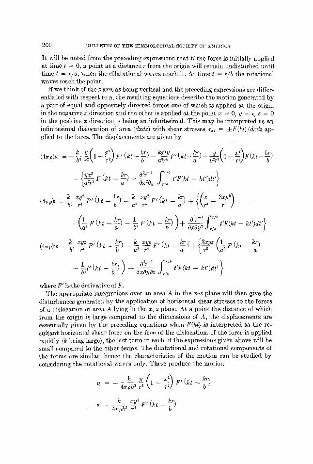
These expressions show that the ground displacements are directly proportional to the time rate of change of the applied forces. Consider a circular dislocation with an initial static shear stress sl on the faces, and assume that slipping star ts at the center of the dislocation and progresses with uniform velocity to the perimeter. During slipping the stress on the face of the dislocation will drop to a value s2

ff a

i

b

Fig. 2. Force on a dislocation as a function of time. a, resultant force on face; b, dis-

F" placement of point with passage of wave; ~ j v t , ~ ' c, velocity; d, acceleration.

C

F 'j ~ r ~ _

depending on sliding friction. The relative motion between the faces of the disloca- tion is brought to rest progressively from the perimeter to the center of the disloca- tion. During this process the stress will drop to essentially zero. Following this the stress will build up to some value s3 as the surrounding material comes to rest, The resultant force on the face of the dislocation, will vary with time essentially as shown in figure 2, a, with successive derivatives as shown in figure 2, b, c, d. The displacement at a point, produced by the passage of the waves, will vary as shown in figure 2, b, the velocity as shown in figure 2, c, and the acceleration as shown in figure 2, d. I t is seen that the rotational wave generates essentially a single displace- ment pulse and a double acceleration pulse, this latter resembling o~e cycle of a sine wave. The dilatationaI wave produces similar pulses traveling at a higher ye!ocity.

202 BULLETIN OF THE SEISMOLOGICAL SOCIETY OF A2CIERICA

The preceding expressions also show that points on the x, z plane do not undeego any motion. This indicates that if the earth's crust were homogeneous and isotropic there would be no motion on the fault plane outside the area of slip. Nonhomo- geneities, and the like, in the earth's crust produce wave reflections and refractions, so that motion does occur on the fault plane at the surface of the ground; but some observations have shown that the intensity of ground motion near the fault plane is less than at adjacent points.

It may also be noted from the preceding expressions that there is a strong direc- tional effect in that the amplitude of motion is very much less in the vicinity of the x axis than in the vicinity of the y axis. This indicates that for vertical slipping on a fault the epieentral region will be shaken with very much less intensity than if the same energy were released by horizontal slipping. It also indicates that more energy would be radiated parallel to the fault for vertical slipping than for horizontal slipping. Both of these effects were reporte d on the occasion of the Arvin-Tehachapi earthquake of July, 1952, which was stated to have been produced by essentially vertical slipping.

THE MECHANISM OF RELEASE

To determine when and where the individual dislocations are released during an earthquake would require a precise knowledge of the state of stress along the fault, the properties of the material, and other facts. This is clearly impossible to achieve; however, the problem may be approached statistically. That is, a probability me- chanism can be postulated that, although not describing precisely the release of each individual dislocation, will describe the average properties of ensembles of dis- locations. Again, there is no way of deriving a precise specification of the statistical problem, but this must be deduced from observations of actual earthquakes, a knowledge of the properties of rock, a knowledge of stress distributions associated with shear dislocations of specified type, and the like. From such considerations the following mechanism is postulated.

First, the average relative slip between the faces of a composite dislocation of area A is taken to be proportional to the square root of A. This statement is to be understood in a probability sense. That is, it is not required that for every composite dislocation the average slip be precisely proportional to the square root of the area of slip; it is only required that the deviations from this rule may be viewed as statistical deviations about a mean and that the statements refer to the relation between the mean slip of all earthquakes of a specified area and that area.

The statement that the average slip is proportional to the square root of the slip area implies that the areas are geometrically similar. Actually this can be true only for slip areas up to a certain size, for the usual strong-motion California earthquakes originate at a ten-mile depth and the extent of the slip area is bounded by the sur- face of the ground. The growth of the slip area is also inhibited because at increasing depths the physical properties of the rock approach those of a material which flows plastically under applied stresses and therefore cannot maintain shear stresses of as great magnitude as the material nearer to the surface, although it undoubtedly can rupture in a brittle manner under suddenly applied shear strains. It is presumed that slip areas of increasing size will be geometrically similar, roughly circular in shape, up to a certain size A1; from size Ai to A2 the shapes of the slip areas are not

PROPERTIES OF STRONG GROUND MOTION EARTHQUAKES 203

geometrically similar; for areas greater than As geometrical similarity again holds, the shapes of the areas being roughly rectangular and differing in length of slip but not appreciably in depth of slip area. For this last case the average slip is propor- tional to the length rather than the square root of the area.

Second, there is required a formulation of the probability of release of disloca- tions. The mechanism that controls the size of the slip area is associated with the distribution of static shear stress along the fault. It is logical to assume that the distribution of shear stress varies quite irregularly over the fault plane, that is, something like a two-dimensional, random, continuous function. As the state of shear strain builds up, the stresses increase until some point reaches the failing stress. This region will then slip and the extent of the slip will be governed by the region of low stress surrounding this point. The state of stress over a rectangular area of fault with dimensions 11 by/2 can be expressed by

T ~ . nTr m ~ = C,~,sm-t~lxsin--[2-y

and as the state of strain builds up, the coefficients C,~ increase until a slip occurs, at which time there is a sudden change in the coefficients. The relative displacement of the two faces of the fault from the unstressed configuration will also be irregular, but will be much smoother than the stress distribution. The relative displacement can also be expressed in a Fourier form:

n~- n?r u = ~ - ' ~ B ~ . s i n - - x s i n

l~ ~ y

It is assumed that the Bran occur in such a way that the frequency of slips of various areas is inversely proportional to the area. That is, the expected number of slips having areas lying between A and A d- dA is proportional to d A / A . As will be seen, such a frequency distribution for the areas agrees well with observations. It is possible, in principle, to compute the detailed behavior of the coefficients C~, and Bran required for such a frequency distribution, and this would give information on the probable distribution of Stress and strain along a fault.

Let the frequency distribution of slip areas A be written

ao 1 f=c =C-x

where a0 is the lower limit of A. The total probability must equal unity, so that

f~ i ~ ~- dx = C log 1 C 3: X0

1

log x~ X0

204 BULLETIN OF THE SEISMOLOGICAL SOCIETY OF AMERICA

where xl is the maximum possible value of x. The frequency distribution of x is therefore

1 1 f - (,)

log x~ x

It may be noted that there must be both an upper limit and a lower limit for x, otherwise log x~/xo becomes infinite and the frequency distribution does not exist.

The mechanism postulated above does not describe the details of a specific earth- quake, but it describes an average process that should agree with the averages of observations. The mechanism is also a simplification in that it does not include the effects of the variation of physical parameters in the earth's crust. In particular, the fact that with increasing depth the physical properties vary from those of an essen- tially linearly elastic solid to those of a material that deforms plastically under slowly applied strains is not included. This means that certain relaxation processes that are undoubtedly operative are not considered. Also, the mechanism excludes from consideration such shocks as may arise from processes other than horizontal slipping along essentially vertical fault planes.

MAGNITUDE AND FREQUENCY

According to the view expressed above, a natural measure of an earthquake is the average slip occurring on the fault. Accordingly, a logarithmic measure of the aver- age slip is taken to define an earthquake, that is, the measure M is related to the average slip by

dS d M -

S

where S is the average relative slip. In integral form this is

= M ( 2 )

Since the average slip is proportional to the square root of the slip area A it follows that

A = Aoe TM

The frequency distribution of earthquakes given by equation (1) states that the relative frequencies are inversely proportional to the area A, so the frequency dis- tribution of shocks in terms of M is

f = ce -2M (3)

Equation (3) may be compared with recorded data on frequency of occurrence of earthquakes. Such data have been presented by Gutenberg and Richter, 2 who give

B. Gutenberg and C. F. Richter, Seismicity of the Earth (Princeton University Press, 1949).

:PROPERTIES OF STRONG GROUND MOTION EARTHQUAKES 205

the observed frequencies of shallow-focus world earthquakes, southern California earthquakes, and New Zealand earthquakes as

log I0N = a + b(8 = M) (3a)

where N is the mean annual number per tenth magnitude, M is the magnitude of a shock as defined by Richter, and the coefficient b is 0.9, 0.88, 0.87, respectively, These values were obtained by plotting log N against M and fitting a straight line to the data. The points fitted the line closely except for magnitudes greater than 8, in which range the observed frequencies fell below the line with an apparent upper limit for M of 8.7. If the preceding equation is put in exponential form, there is obtained for world earthquakes, southern California earthquakes, and New Zealand earthquakes, respectively,

-2.07M N - - - - Vie

-2.02M N ~ c2e

N ~ C3e -2"OOM

It is seen that equation (3) fits the data within the limits of observational accuracy. It is also seen from the foregoing that the measure of an earthquake as defined

in this paper may be identified with the magnitude defined by Richter. He defined the magnitude as being the logarithm of the maximum trace amplitude recorded by a certain type of seismograph located 100 kilometers from the epicenter of an earth- quake. It will be shown later that the maximum acceleration is proportional to the square root of the area of slip, and hence that the physical interpretation of the two measures is the same.

ENERGY RELEASED

The strain energy stored in a solid by a single shear dislocation is equal to the work that must be expended by the shear stresses acting on the faces bf the dislocation in producing the relative displacement of the faces. The strain energy stored by a dislocation of area a~ is, thus,

E , = ½ j.~,S,/a, where T= is the shear stress acting on the face and S~ is the relative displacement (variable) of the two faces. The failing stress T is the same for all dislocations, so if Sn and a~ are the average slip and average area the total energy released by N dislocations is

N

E = E E ~ = ~_,CnTS-.a,~= C N

The total energy released is thus proportional to the number N of dislocations released. The number N is proportional to the area of slip multiplied by the average slip over A, so

206

or

BULLETIN OF THE SEISMOLOGICAL SOCIETY OF AMERICA

E = C I A ~

Z = Ce T M (4)

This relates the energy released to the magnitude of the shock. Equation (4) applies only to the smaller geometrically similar slip areas. For

example, a small slip area will have longitudinal and vertical dimensions approxi- mately equal, and increasingly larger slip areas will be geometrically similar to this up to a certain point. The vertical dimensions of slip areas are limited in that a slip originating at a ten-mile depth can extend upward only ten miles, and because of the changing physical properties of the earth's crust with depth, the slip is limited in the downward direction also. This means that the slip areas of very large earth- quakes increase principally by an elongation of the area and that the vertical di- mension of the slip area does not increase proportionally. Such slip areas are not geometrically similar to the smaller slip areas, and this must be taken into account when the energy released is computed. For geometrically similar slip areas the aver- age slip is proportional to the length of the fault. For the smaller shocks this varies as

However, for very large geometrically similar shocks where the slip area receives no restraint from material above or below, the length is proportional to the area, so that

S = C " A

In this case the total energy must be written

E = Ce 4~ (4a)

There is, of course, a transition region between the limits of applicability of equa- tions (4) and (4a), and the latter presumably applies only to very large shocks.

The foregoing expressions for energy released may be compared with those de- rived by an alternate method by Gutenberg and Richter2 Consider that at the epi- center the radiated energy arrives in a sinusoidal wave train with maximum acceler- ation a0 and duration to, that is, consider the actual accelerogram to be replaced by an equivalent sinusoidal wave train. Assuming the total energy released to be pro- portional to the energy reaching the epicenter will then give

E = Ctoao 2

where ao is the maximum acceleration at the epicenter. From the recorded ground accelerations it is found that the following empirical expression relates ao with M

M = 2.2 A- 1.8 log10 ao or

ao --- Cle I"28M

a B. Gutenberg and C. F. Richter, "Earthquake Magnitude, Energy, In tens i ty and Accelera- t ion," Bull. Seism. Soc. Am., 32:163-191 (1942).

PROPERTIES OF STRONG GRO,UND MOTION EARTHQUAKES

As shown below, the duration may be taken to be \

~0 = '.,~2~ f ~ M / 2

207

These values give for the energy released

E = Ce 3"°6M (4b) i

which agrees with equation (4). The foregoing analysis does not include the energy carried in the long-period

components tha t are found in very large shocks. To allow for this, Gutenberg and Richter apply the correction factor e M, thus obtaining

E = Ce 4'°sM (4c)

which agrees with equation (4a).

AREAS OF SLIP

According to the foregoing analysis, the total area of relative slip along a fault is proportional to the square of the maximum slip. In terms of the magnitude the area of slip is thus

A = Aoe 2M (5)

This expression should be understood in a probability sense, namely, that on the average shocks of magnitude M will have an area A corresponding to equation (5). As was seen when discussing equation (1), there must be an upper limit for the area A and also a lower limit. The lower limit is the area of the smallest individual shear dislocation tha t can be released under the conditions applying to an earthquake fault; the upper limit is imposed by the fact that earthquake faults are of finite extent.

The areas corresponding to different values of M can be compared by means of equation (5), for example,

A1 e2(M1-M~) A2 - (6)

To investigate the implications of this equation let the E1 Centro shock of May 18, 1940, be considered a typical 6.7 magnitude earthquake. Judging from the visible surface slip, it is estimated that this shock had a slip area of approximately 40 × 20 = 800 square miles. Using this as a base, the areas of shocks of other magnitudes are given by

A = 800e 2(M-6"7)

This gives for a shock of magnitude M = 0, an area of slip

A0 = 0.0{)12 sq. miles

which is equivalent to a circular area of 210 feet diameter. The relative slip asso-

208 BULLETIN OF THE SEISMOLOGICAL SOCIETY OF AMERICA

elated with an area of 210 feet diameter may be estimated as follows. The average slip varies with magnitude according to equation (2). For geometrically similar shocks the maximum relative slip is given by the same expression, tha t is,

~ ~0 CM

The maximum surface slip of the E1 Centro shock was approximately 15 feet, and if the maximum subsurface slip for a 6.7 magnitude, tha t is, the upper bound of a range of geometrically similar shocks, is taken to be the same, the slip for shocks

of smaller magnitudes is given by

S = 15e (~-6'7) (7)

For M = 0 this gives a maximum slip of 0.25 inch. This indicates tha t the typical smallest dislocation is one of area corresponding to approximately 210 feet in diam- eter with a maximum relative slip between faces of 0.25 inch.

If the preceding equations are applied to a shock of 8.2 magnitude, such as the San Francisco earthquake of 1906, there is obtained a total area of slip equal to 300 X 55 miles. The surface slip of the 1906 shock disappeared into the ocean north of San Francisco, but it appears tha t the total slip area was of the order of magnitude

of the above-mentioned figure. The total movement in California can be estimated by means of the foregoing

equations. If the mean annual frequency distribution of shocks in California is taken to be the same per unit area as for southern California, 4 there is obtained

f = 0.00086e 2(s'7-M) .

The area of slip per shock according to the preceding calculation is:

A = 0.0012e TM sq. miles

The average relative slip over the area is approximated by one-half the maximum

slip, or 1 i = ~(0.25)e inches

The total mean annual slipping is given by the integral of ( f A G ) , and if this is as- sumed to be distributed uniformly over faults 30 miles deep and 700 miles long there is obtained for the mean annual relative shearing motion of the east and west boun-

daries of the state

f0 8.7 ( 0 . 0 0 0 8 6 ) ( 0 . 0 0 1 2 ) ½ ( 0 . 2 5 ) e 17 .6 e M (30)(700) - d M = 2.2 inches per year

This may be compared with the estimate of a mean annual relative motion of approximately 2 inches per year tha t is based on triangulation surveys.

Gutenberg and Richter, Seismicity of the Earth.

PROPERTIES OF STRONG GROUND MOTION EARTHQUAKES 209

The average duration of the strong motion at the epicenter can be estimated from the motion of a point along the fault. Since such an element of material under- goes a displacement it must be subjected to a force that accelerates and decelerates. If similarity between earthquakes is assumed, the force is similar for earthquakes of various magnitudes, differing only in duration. Thus the motion of the point can be written

d2S d ( t , / k ) 2 - F( t ' ) ( t ' / k = t, 0 < t' < t , ')

.'. I~2SI = C

t l /

tl = C1 ~ = C2~ /~

where $1 is the maximum slip. The duration estimated from seismograms by Guten- berg and Richter 5 is

lOgloto = a + M 4

or

to = Ce M/l'9~

The foregoing values of slip areas, and the like, are not exact, but are only ap- proximations that are used to show that the formulas give reasonable values when applied to the limits of their ranges and that they are not inconsistent with obser- vations.

ACCELEROGRAMS DERIVED FROM STRESS PULSES

When the stresses along a fault are released, they radiate stress pulses which after reflection and refraction are recorded on an accelerogram on the surface of the ground. It will be assumed that the pulses reaching the strong-motion accelerom- eter are similar to those sent out by the release of a single stress dislocation, or, more particularly, that each pulse records as one cycle of a sine wave. It is not essential that the pulse be exactly one cycle of a sine wave; this is only a computational con- venience. However, it is essential that the pulse be double-looped, for it will be shown that it is not possible to form a typical accelerogram with single-looped pulses such as one-half cycle of a sine wave. It is also necessary that the swarm of pulses have various wave lengths, for it is not possible to form an accelerogram with the properties of recorded accelerograms with a swarm of pulses all of the same wave length. As will be seen, the pulses required are predominantly of 2/10-second wave length.

It is assumed that during an earthquake the motion recorded by an accelerom- eter is composed of a swarm of pulses random in time. To determine the required distribution of pulse wave lengths and amplitudes the following method of analysis

See reference in fn. 3 above.

2 1 0 BULLETIN OF Tt{E SEISMOLOGICAL SOCIETY OF AMERICA

is used. A recorded accelerogram is considered to be a random continuous function and an earthquake is considered to be a random sample from a parent population. The characteristics of a random continuous function (accelerogram) are exhibited by its energy spectrum. The spectra have been computed for recorded strong-motion aecelerograms and the average of these spectra is taken to be the spectrum of the parent population of strong-motion earthquakes. The distribution of pulse wave lengths, amplitudes, and numbers is determined so that the spectrum of the parent population of pulses is the same as the above-mentioned average recorded earth- quake spectrum.

Consider a swarm of pulses, every one of which is represented by the acceleration

f (k ( t -- t~)) = s i nk ( t - - O) O - ~ < t < O +

where the times of occurrence 0 are randomly distributed over an interval of time. If a certain number n of such pulses are superimposed at random, they will form an accelerogram the energy spectrum of which is given by

(f )' (f )' F(k, ,, O) = ~ f (k( t -- 0 ,))s in , tdt + ~ f (k( t -- 0.)) cos , t dt

This will, in general, be an irregular curve, but the average of a large number of spectra from different sets of n pulses will approach a smooth curve that character- izes the population from which the pulses were taken. To compute the average spectrum it is only necessary to integrate the foregoing expression with respect to O, since the probability of 0 is constant with respect to time. When this is done, there is obtained for the average spectrum

F(l , = 2 n

o r

n / S i n r ~ 2 F ( k , . ) = 2 (S)

where r is the ratio of the wave length being considered on the spectrum to the wave length of the pulses. This is shown in figure 3, where the square root of the spectrum is drawn. In the case of one-half sine pulses, that is, single-loop pulses, the average spectrum is

The square root of this curve is drawn also in figure 3. These curves are typical in that the double-looped pulses produce a humped curve, whereas the single-loop pulses do not.

PROPERTIES OF STRONG GROUND MOTION EARTHQUAKES 211

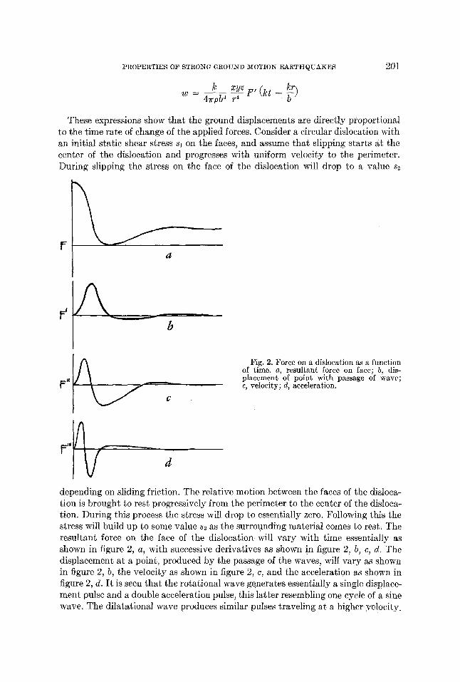
I f an accelerogram is formed by the random superposition of pulses of a var ie ty of wave lengths and amplitudes, the mathemat ica l expectation of the spectrum is

/ I/e~ sin r \2 I n k - (10) F(k, ~) =2 ~ ~

1

where nk is the number of pulses in the population which have wave length k, and Ak is the ampli tude of these pulses.

2

CO5

0.5 1.0 1.5 2.0 2.5 3.0

Period in Seconds (T = 0.2/r )

Fig. 3. Pulse spectra.

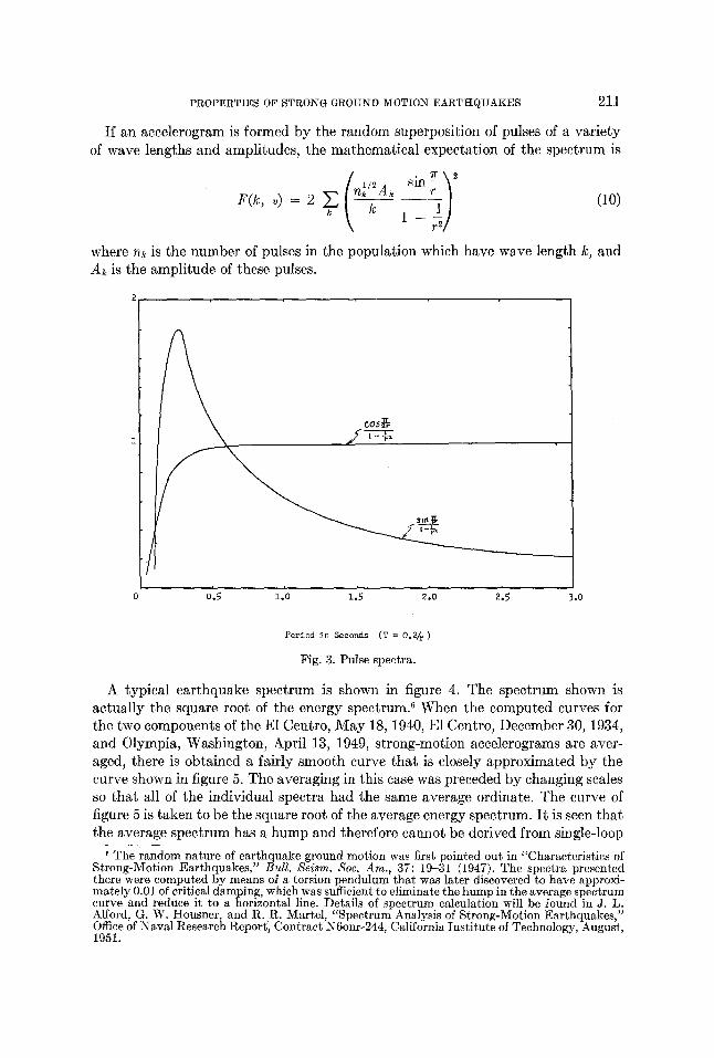
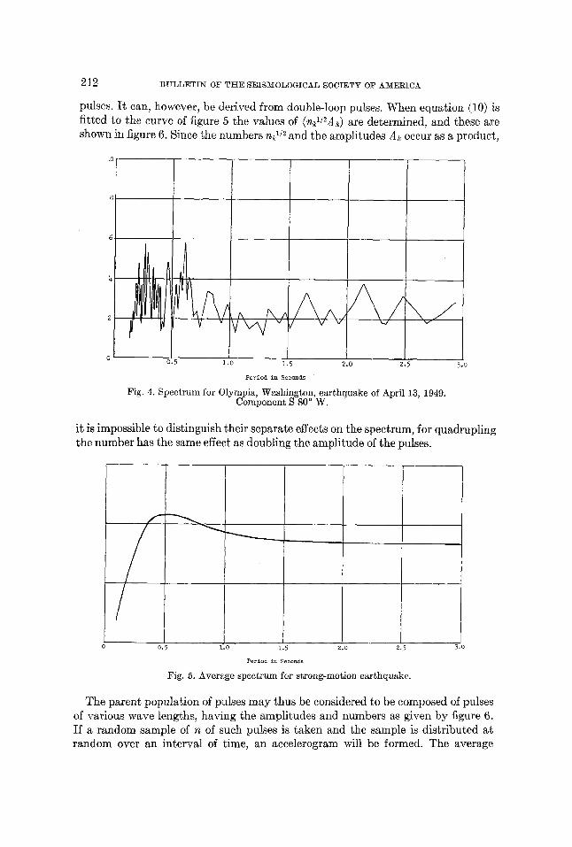
A typical ear thquake spectrum is shown in figure 4. The spectrum shown is actual ly the square root of the energy spectrum. 6 When the computed curves for the two components of the E1 Centro, M a y 18, 1940, E1 Centro, December 30, 1934, and Olympia, Washington, April 13, 1949, strong-motion accelerograms are aver- aged, there is obtained a fairly smooth curve tha t is closely approximated by the curve shown in figure 5. The averaging in this case was preceded by changing scales so tha t all of the individual spectra had the same average ordinate. The curve of figure 5 is taken to be the square root of the average energy spectrum. I t is seen tha t the average spectrum has a hump and therefore cannot be derived from single-loop

6 The random nature of earthquake ground motion was first pointed out in "Characteristics of Strong-Motion Earthquakes," Bull. Seism. Soc. Am., 37:19-31 (1947). The spectra presented there were computed by means of a torsion pendulum that was later discovered to have approxi- mately 0.01 of critical damping, which was sufficient to eliminate the hump in the average spectrum curve and reduce it to a horizontal line. Details of spectrum calculation will be found in J. L. Alford, G. W. Housner, and R. R. Martel, "Spectrum Analysis of Strong-Motion Earthquakes," Office of Naval Research Report~, Contract N6onr-244, California Institute of Technology, August, 1951.

212 B U L L E T I N OF THE: SEISMOLOGICAL SOCIETY OF AMERICA

pulses. It can, however, be derived from double-loop pulses. When equation (10) is fitted to the curve of figure 5 the values of (nkll2Ak) are determined, and these are shown in figure 6. Since the numbers nk m and the amplitudes Ak occur as a product,

ill, vAv, \ v /

0.5 1.0 1.5 2.0 Z.5

Period in Seconds

Fig. 4. Spectrum for Olympia, Washington, earthquake of April 13, 1949. Component S 800 W.

5.o

it is impossible to distinguish their separate effects on the spectrum, for quadrupling the number has the same effect as doubling the amplitude of the pulses.

0.5 Lo L5

Period in Second~

2.0 2,5

Fig. 5. Average spectrum for strong-motion earthquake.

3 .0

The parent population of pulses may thus be considered to be composed of pulses of various wave lengths, having the amplitudes and numbers as given by figure 6. If a random sample of n of such pulses is taken and the sample is distributed at random over an interval of time, an aceelerogram will be formed. The average

FROFERTIES OF STRONG GROUND I~OTION EARTI:IQUAKES 213

spectrum of a large number of accelerograms obtained in this way will approach the spectrum of figure 5. A sample accelerogram obtained in this way will thus have the characteristics of actual recorded accelerograms so far as these are random con- tinuous functions.

A sample accelerogram was constructed by distributing 584 pulses over a 10- second interval, allotting 292 to each 5-second interval. To simplify the computa-

0 0.5 1.0 1o5 2.0 2.5

Period of Pulse in Seconds

Fig. 6. Distribution of nA~/k.

tions, the numbers and amplitudes of pulses for 1/10-second increments of wave length were selected so that the proper n~12Ak/k~ was obtained, and these were dis- tributed at random by means of a table of random numbers. This procedure will give a somewhat more uniform-looking accelerogram than would be obtained if the pulses had been selected at random from the population and distributed at random over a 10-second period. The resulting accelerogram is shown in figure 7. For com- parison there is shown a portion of the Olympia, Washington, accelerogram in figure 8. It is seen that the two are very similar in appearance even to the degree that on the average they cross the axis the same number of times per second.

It should be noted that the preceding method of superposing the pulses actually corresponds to the time of strong motion only, that is, when very large numbers of pulses are arriving. The earlier and later portions of recorded accelerograms may show many fewer pulses arriving. Also, one would infer that the random arrival of the longer-period pulses is a consequenco of reflections and refractions through var- ious strata; there is a similar effect on the short-period pulses. However, the char- acter of the accelerogram depends largely on the predominant pulses having periods in the neighborhood of 0.2 second, and this is true for all the recorded strong-motion

214 B U L L E T I N OF T H E S E I S M O L O G I C A L SOCIETY OF A M E R I C A

llr Vv v

0 1 2 3 4 5 6

Tlme in Second~

v l l vv 7 8 9 zo

Fig. 7. Aeeelerogram formed by random superposition of pulses.

1 2 3 h 5 6 ? 6 9 zo

Time in Seconds

Fig. 8. Portion of Olympia, Washington, aecelerogram.

aceelerograms of large earthquakes, even though the shocks occurred at widely separated locations and had different types of slipping. It thus appears unlikely that this similarity can be attributed to reflections and refractions, but it may be a con- sequence of irregularities of stress release along the fault; for example, the original stress along the fault may be nonuniform or the stress may not be uniform during slipping, and the effects of these could be expected to be similar for different shocks. The effects of these short-period components would not, of course, be apparent on displacement records.

PROPERTIES OF STRONG GROUND MOTION ]~ARTttQUAKES 215

MAXIMUM ACCELERATIONS

When an accelerogram is constructed with a set of pulses in the foregoing manner it is found that, to a considerable degree, the pulses cancel each other and that the maximum accelerations are the result of fortuitous superpositions of pulses. If a second accelerogram is constructed using the same set of pulses, it will differ from the first because of the random superposition of the pulses. However, if a large number of accelerograms are constructed using the same set of pulses, they will have certain average properties; for example, there will be an average maximum acceleration and the maximum accelerations of the individual accelerograms will deviate from the average with a certain statistical distribution. In what follows, the references to accelerations are to the average properties.

When the average energy spectrum is calculated for a given distribution of pulses, its ordinates, as shown by equation (10), are proportional to (hA2), where n is the number of pulses and A is the amplitude. On the other hand, if accelerograms are constructed from the pulses and the spectra computed for these, the average spec- trum will have ordinates proportional to the square of the maximum acceleration. Therefore, the maximum acceleration a is proportional to the amplitude of the pu]ses and to the square root of the number of pulses, that is,

a = K(n) I /2A

where the number n is the pulse density at the point where the accelerations are measured, that is, the number of pulses per unit time. If an increment of fault area dx dh is considered to radiate pulses at a rate n per unit area, the maximum accelera- tion at a specified point on the surface of the ground will have a maximum accelera- tion

= K ( n dx dh)l/ZA (11)

If the point on the surface of the ground is at such a distance from the fault that the radiation can be considered to come from a point source, the maximum accelera- tion recorded will be the cumulative acceleration from the total area that is radiat- ing, that is,

a ~ = K ~ J J n A 2 dx dh (12)

If the radiation is the same from all points on the fault area, the maximum accelera- tion will be

a = C A (N) I/2

where N is the rate of pulse radiation of the entire fault area and A is the amplitude. N is directly proportional to the area, so the maximum acceleration is proportional to the square root of the fault area. In terms of the magnitude

a = C l e M (13)

This is essentially Richter's definition of magnitude, in terms of acceleration instead of displacement, which is thus a measure of the area of slip.

216 BULLETIN OF THE SEISMOLOGICAL SOCIETY OF AMERICA

For points relatively close to the fault it is not correct to assume point-source radiation, but the area of the fault must be taken into account. A qualitative inves- tigation of this effect may be made as follows. Consider a fault of length 21 and vertical dimension h0, each point of which is radiating pulses according to equation (11). Furthermore, let the effect of the position of the point on the surface of the ground, where the accelerations are measured, relative to the point on the fault be de- scribed by the inverse-square law with cosine correction as given by Gutenberg and Richter, 7 that is,

h (14) a = K (n dx dh)~/2A x2 d- y~ -4- h '2

where x, y, h are the coSrdinates of the point on the surface of the ground with respect to the radiating point. The effect of the radiation from the fault area can be approximated by considering the radiation from a line of length 2l at an equivalent depth h if the strength of the radiation is taken to be proportional to h0. If, then, the maximum acceleration is calculated for the line in accordance with equations (12)

and (14), there is obtained

, oho h 2 + + (x - 1)(h 2 + y2) 1/2_

( x - l ) 2 + h 2 + y 2 (15)

x + 1 _tan-1 x - - 1 %1/~ + tan -1 %/h' -t- Y' V h 2 _}_ yi)

i

where x, y, h are the coSrdinates of the point on the surface of the ground as meas- ured in a coSrdinate system with origin at the center of the line, x and y being respectively parallel and perpendicular to the line and h being the vertical distance from the center of the line to the surface of the ground. Equation (15) describes the variation of seismicity over the surface of the ground. When 1 -+ 0 with (a011/2) constant, there is obtained for point-source radiation

h (16) a = ~0(h0/) 1/2 (x 2 -t- y2 _}_ h 2)

which agrees with equation (14). According to equation (13), a = Cle i and according to equation (4) the energy

released is E = C2e T M SO a is proportional to the cube root of the energy, and equa-

tion (16) can be written h (16a)

a = C(E) 1/3 x~ _]_ y2 q_ h 2 "

The same equation is derived by Gutenberg and Richter s by using empirical equa- tions based on observations. For very large earthquakes equation (4a) shows E ---- C2e 4M, so the exponent in (16a) should be 1/4 instead of 1/3. This reflects the

7 B. Gutenberg and C. F. Richter, "Earthquake Magnitude, Energy, Intensi ty and Accelera- tion," Bull. Seism. Soc. Am. , 32:163-191 (1942).

8 Ibid.

PROPERTIES OF STRONG GROUND MOTION EARTHQUAKES 217

fact tha t for very large shocks a significant part of the energy is released in long- period waves which have very small accelerations.

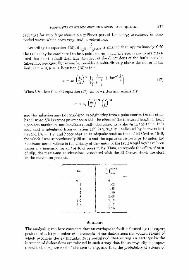
1 According to equation (15), if (h: + y2)1/~ is smaller than approximately 0.20

the fault may be considered to be a point source, b u t i f the accelerations are meas- ured closer to the fault than this the effect of the dimensions of the fault must be taken into account. For example, consider a point directly above the center of the fault at x = 0, y = 0. Equat ion (15) is then

a = a0 (17) ~l h

When 1/h is less than 0.2 equation (17) can be written approximately

and the radiation may be considered as originating from a point source. On the other hand, when 1/h becomes greater than this the effect of the increased length of fault upon the maximum accelerations rapidly decreases, as is shown in the table. I t is seen that a calculated from equation (17) is virtually unaffected by increase in l beyond l /h = 1.2, and hence that an earthquake such as tha t of E1 Centre, 1940, for which 1 was approximately 20 miles and the equivalent h perhaps 10 miles, the maximum accelerations in the vicinity of the center of the fault would not have been materially increased for an l of 40 or more miles. Thus, as regards the effect of area of slip, the maximum accelerations associated with the E1 Centre shock are close to the maximum possible.

o

l/h ao

0 .2 .4 .6 .8

1.0 1.2 co

0 .62 .85 .99

1.08 1.13 1.17 1.25

SUMMARY

The analysis given here considers tha t an earthquake fault is formed by the super- position of a large number of incremental shear dislocations the sudden release of which produces the earthquake. I t is postulated tha t during an earthquake the incremental dislocations are released in such a way that the average slip is propor- tional to the square root of the area of slip, and that the probabili ty of release of

218 BUI-~]~TIN OF TI tE SF-~S~OLOGICAL SOCIETY OF AMERICA

individual incremental dislocations is such that the probability of a total slip area A is inversely proportional to A. With these two postulates a frequency distribution of earthquakes is derived that agrees with observed data; the Richter magnitude is shown to be essentially a logarithmic measure of the average slip on a fault; and an expression is derived for the energy released by an earthquake that agrees with that derived from consideration of the energy carried in a wave train. Expressions are derived also for the areas of slip during earthquakes, the maximum relative slip, and the average annual, over-all shearing distortion of the state of California and these are in satisfactory agreement with observed behavior. I t is assumed that an accelerogram is formed by the superposition of a large number of elemental accelera- tion pulses random in time. It is shown that this agrees with recorded aecelerograms, and an accelerogram composed in this fashion is shown to have the characteristics of actual recorded aecelerograms. It is also shown that the maximum ground accelera- tions in the vicinity of the center of the fault, so far as they are dependent upon the size of the slip area, have essentially reached their upper limits for shocks with areas of slip approximately equal to that associated with the E1 Centro earthquake of 1940.

CALIFORNIA INSTITUTE OF TECHNOLOGY PASADENA~ CALIFORNIA