proportional, integral, and derivative controller design part 1 · 2020-04-20 · controller...
TRANSCRIPT
A SunCam online continuing education course
Proportional, Integral, and Derivative Controller Design Part 1
by
Peter J Kennedy
291.pdf

Proportional, Integral, and Derivative Controller Design Part 1
A SunCam online continuing education course
www.SunCam.com Copyright 2017 Peter J. Kennedy Page 2 of 40
1.0 Introduction: In this course, the design and applications of Proportional -plus- Integral -plus- Derivative (PID) controller’s is discussed. PID control is a technique used extensively in feedback control systems. Its origins date back to the 19th century, being used for governor speed control, and since then in numerous applications with a wide variety of actuators and sensors. The controller is simple structure; being the sum of three terms as the name implies. Its configuration is illustrated in Figure 1.0. The PID structure provides for a fairly-wide range of tuning adjustment in a feedback control loop, especially for relatively simple processes. Some familiarity with feedback control may help in providing a better understanding of the course material. References [1, 2] provide excellent coverage of PID controller design as included in this course. Essential aspects of feedback control are included, but one might also review references on the subject [3, 4] or Suncam Course 182.
Figure 1.0 Functional Block Diagram PID Controller
PID controllers are used in many control applications; possibly being the most common form of feedback control compensation. With feedback control, the output state of a physical system to be controlled—referred to as the plant, process, or load—is measured by a sensor. The measured state is fed back and compared to a desired state. The terminology for the desired state varies depending on the application; often termed set point in process control, a reference signal in circuit design, or a command input from an outer control loop. The controller determines the difference between the measured and desired state; the control loop error, to generate a control signal that reduces the error. This equates to a negative feedback control loop; central to feedback control theory. A PID uses the error, it’s integral and derivative to derive a control signal driving the error to a null state. The controller can be structured in many configurations; P-only, PI, PD, PID, plus others to be discussed. PID control is central to most process control systems; but can also be found in numerous applications other than process control ranging from positioning control loops to pointing, tracking and platform stabilization control loops. The PID can also be integrated with
291.pdf
Proportional, Integral, and Derivative Controller Design Part 1
A SunCam online continuing education course
www.SunCam.com Copyright 2017 Peter J. Kennedy Page 3 of 40
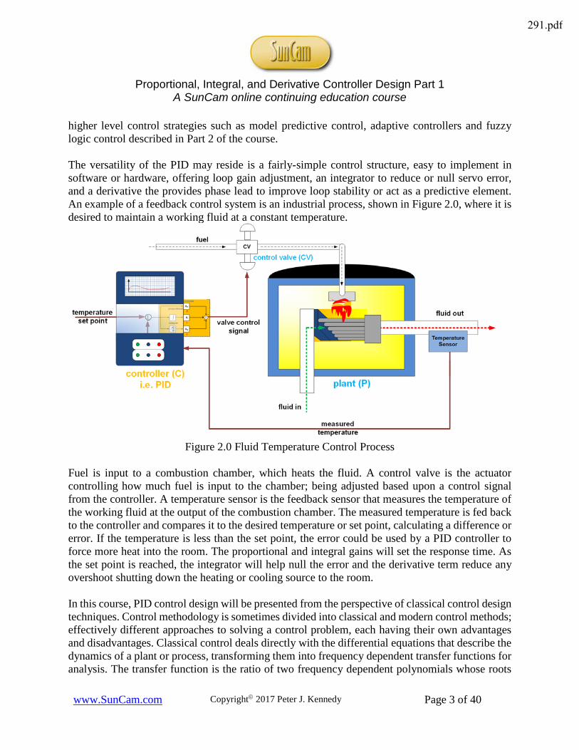
higher level control strategies such as model predictive control, adaptive controllers and fuzzy logic control described in Part 2 of the course. The versatility of the PID may reside is a fairly-simple control structure, easy to implement in software or hardware, offering loop gain adjustment, an integrator to reduce or null servo error, and a derivative the provides phase lead to improve loop stability or act as a predictive element. An example of a feedback control system is an industrial process, shown in Figure 2.0, where it is desired to maintain a working fluid at a constant temperature.
Figure 2.0 Fluid Temperature Control Process
Fuel is input to a combustion chamber, which heats the fluid. A control valve is the actuator controlling how much fuel is input to the chamber; being adjusted based upon a control signal from the controller. A temperature sensor is the feedback sensor that measures the temperature of the working fluid at the output of the combustion chamber. The measured temperature is fed back to the controller and compares it to the desired temperature or set point, calculating a difference or error. If the temperature is less than the set point, the error could be used by a PID controller to force more heat into the room. The proportional and integral gains will set the response time. As the set point is reached, the integrator will help null the error and the derivative term reduce any overshoot shutting down the heating or cooling source to the room. In this course, PID control design will be presented from the perspective of classical control design techniques. Control methodology is sometimes divided into classical and modern control methods; effectively different approaches to solving a control problem, each having their own advantages and disadvantages. Classical control deals directly with the differential equations that describe the dynamics of a plant or process, transforming them into frequency dependent transfer functions for analysis. The transfer function is the ratio of two frequency dependent polynomials whose roots
291.pdf
Proportional, Integral, and Derivative Controller Design Part 1
A SunCam online continuing education course
www.SunCam.com Copyright 2017 Peter J. Kennedy Page 4 of 40
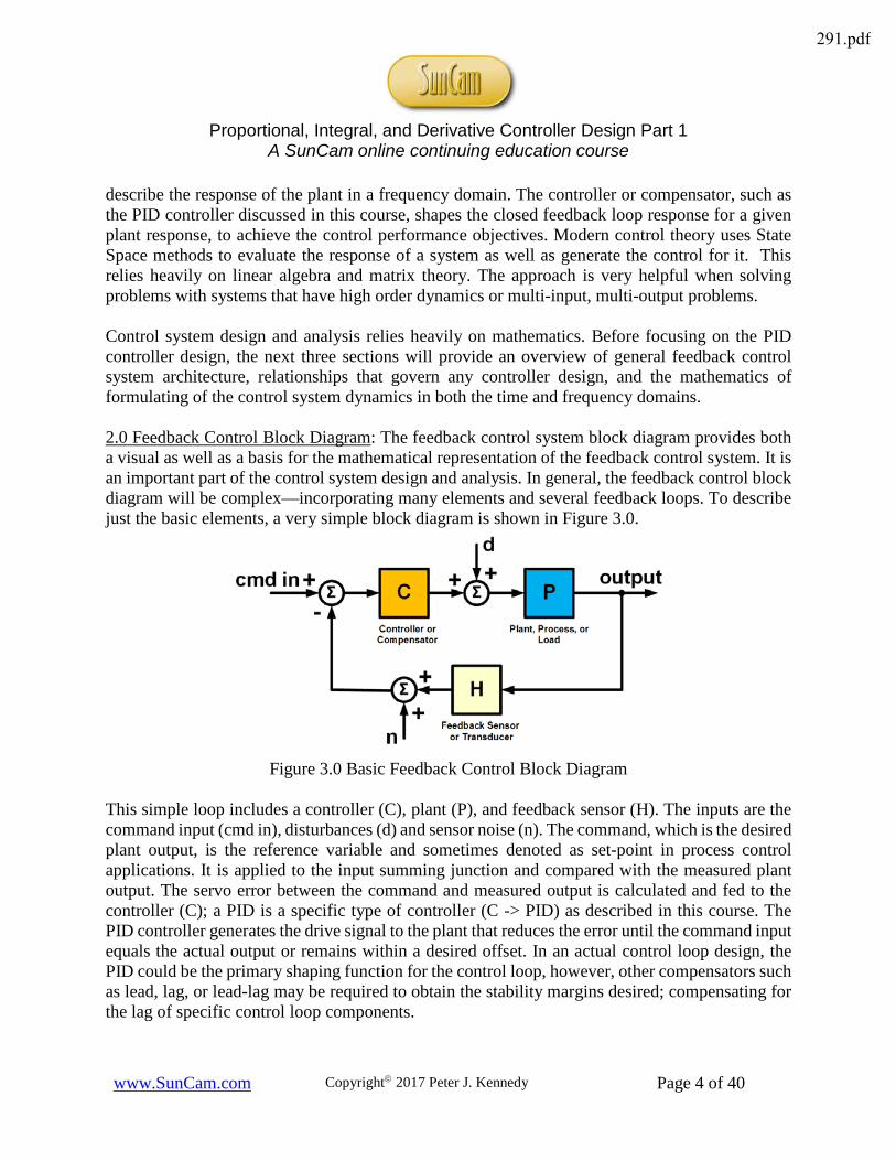
describe the response of the plant in a frequency domain. The controller or compensator, such as the PID controller discussed in this course, shapes the closed feedback loop response for a given plant response, to achieve the control performance objectives. Modern control theory uses State Space methods to evaluate the response of a system as well as generate the control for it. This relies heavily on linear algebra and matrix theory. The approach is very helpful when solving problems with systems that have high order dynamics or multi-input, multi-output problems. Control system design and analysis relies heavily on mathematics. Before focusing on the PID controller design, the next three sections will provide an overview of general feedback control system architecture, relationships that govern any controller design, and the mathematics of formulating of the control system dynamics in both the time and frequency domains. 2.0 Feedback Control Block Diagram: The feedback control system block diagram provides both a visual as well as a basis for the mathematical representation of the feedback control system. It is an important part of the control system design and analysis. In general, the feedback control block diagram will be complex—incorporating many elements and several feedback loops. To describe just the basic elements, a very simple block diagram is shown in Figure 3.0.
Figure 3.0 Basic Feedback Control Block Diagram
This simple loop includes a controller (C), plant (P), and feedback sensor (H). The inputs are the command input (cmd in), disturbances (d) and sensor noise (n). The command, which is the desired plant output, is the reference variable and sometimes denoted as set-point in process control applications. It is applied to the input summing junction and compared with the measured plant output. The servo error between the command and measured output is calculated and fed to the controller (C); a PID is a specific type of controller (C -> PID) as described in this course. The PID controller generates the drive signal to the plant that reduces the error until the command input equals the actual output or remains within a desired offset. In an actual control loop design, the PID could be the primary shaping function for the control loop, however, other compensators such as lead, lag, or lead-lag may be required to obtain the stability margins desired; compensating for the lag of specific control loop components.
291.pdf

Proportional, Integral, and Derivative Controller Design Part 1
A SunCam online continuing education course
www.SunCam.com Copyright 2017 Peter J. Kennedy Page 5 of 40
The dynamics of each block can be expressed in the time or frequency domain. The time domain is very useful for simulating the loop response, and evaluating performance as a function of time. A set of differential equations—which can include non-linear terms—are used to describe the dynamics for each block. The frequency domain is excellent for linear analysis. The gain of each element can be characterized as a function of frequency; effectively making each element a frequency dependent gain. The output response can be evaluated as a function of frequency, and the controller adjusted in the frequency domain, to improve the loop performance. 3.0 Time and Frequency Domain Representations of Loop Dynamics: The plant dynamics are normally described by a set of differential equations and functions for elements that are non-linear in time or multi-variable dependencies. If the plant is linear or can be linearized about an operating point, the frequency domain response can be described by using the Laplace transform or a differential operator. The frequency domain is important for analysis and design; as used in ensuing sections. 3.1 Frequency Domain Definitions: The Laplace transform of a time dependent variable f(t) is defined as:
∫∞
⋅−=0
)()( dtetfsF ts
This integral exists for the complex variable s=σ+jω with any real part σ>0. The variable ω=2πf where ‘f’ is frequency in hertz. Differentiating the right-hand side of this expression n times with respect to time, results in the important relationship:
∑∫=
−−∞
⋅− ⋅−=n
k
knkntsn fssFsdtetf1
1
0
)0()()(
A differentiated function in time is algebraically related to its transform as L[fn(t)]->snF(s) where ‘L’ denotes the Laplace transform. The summation term on the right accounts for the initial conditions of each differentiated term. For frequency analysis, initial conditions are often assumed to be zero so that:
0conditionsinitialfor)()(0
==∫∞
⋅− sFsdtetf ntsn
Two important operator relationships, as listed in Table 1.0, can be derived from this expression.
Table 1.0 Laplace Transform Derivative and Integral Operator Transform Transform Notation Notes
Derivative )()(0
sFsdtetf ts ⋅=∫∞
⋅− )())(( sFstfL ⋅>−
Integral )(1)(0
sFs
dtetf tsI ⋅=∫
∞⋅− )(1))(( sF
stfL ⋅>−∫ ∫
∞
=0
)()( dttftf I
291.pdf
Proportional, Integral, and Derivative Controller Design Part 1
A SunCam online continuing education course
www.SunCam.com Copyright 2017 Peter J. Kennedy Page 6 of 40
The integral relation is obtained, noting the derivative of the integral is the function, so that:
)(1)()()()()(00
sFs
sFsFdtetfsFsdtetf Its
Its
I ⋅=∴==⋅= ∫∫∞
⋅−∞
⋅−
The significance of these relationships is they allow differential equations to be converted to algebraic expressions—similar to the use of differential operators. The inverse Laplace transform can be used to convert a frequency domain function back to one in the time domain. The inverse transform is given by:
∫∞+
∞−
⋅
⋅⋅=
jc
jc
ts dsesFj
tf )(2
1)(π
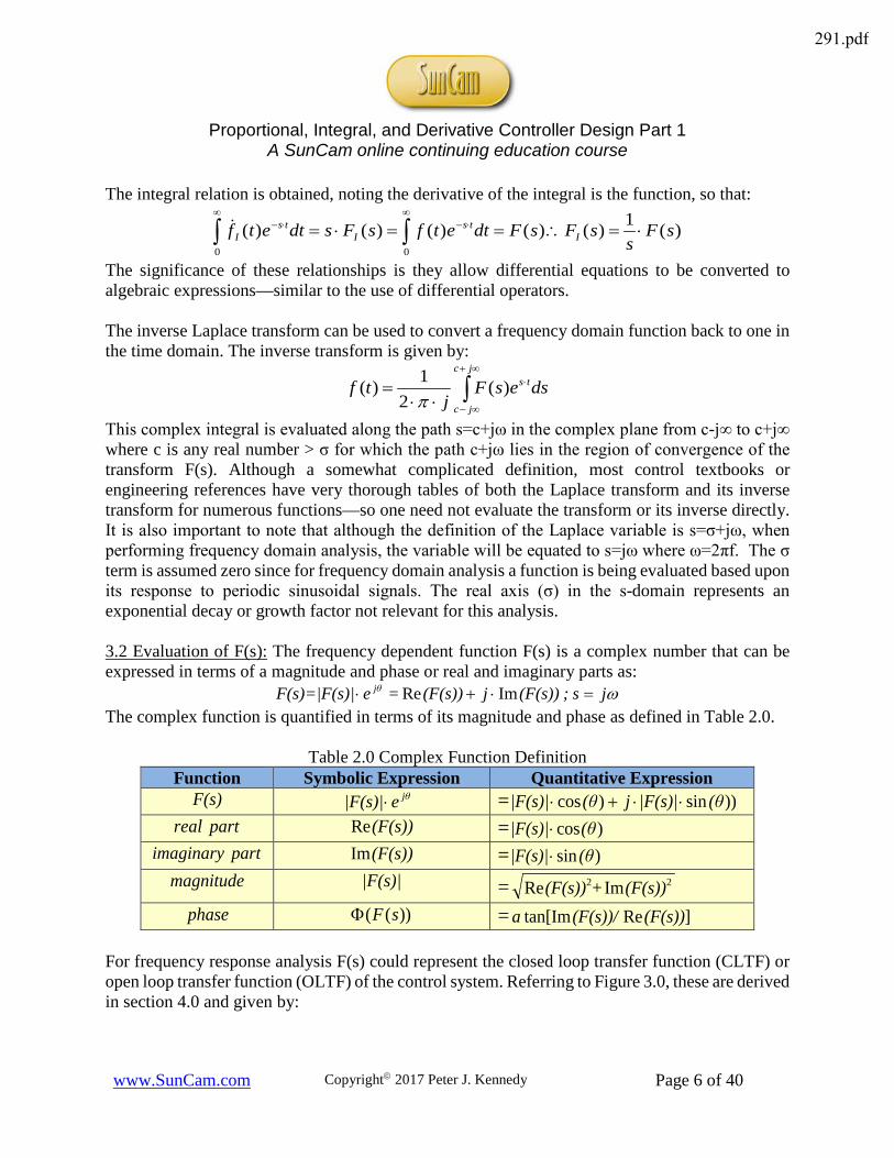
This complex integral is evaluated along the path s=c+jω in the complex plane from c-j∞ to c+j∞ where c is any real number > σ for which the path c+jω lies in the region of convergence of the transform F(s). Although a somewhat complicated definition, most control textbooks or engineering references have very thorough tables of both the Laplace transform and its inverse transform for numerous functions—so one need not evaluate the transform or its inverse directly. It is also important to note that although the definition of the Laplace variable is s=σ+jω, when performing frequency domain analysis, the variable will be equated to s=jω where ω=2πf. The σ term is assumed zero since for frequency domain analysis a function is being evaluated based upon its response to periodic sinusoidal signals. The real axis (σ) in the s-domain represents an exponential decay or growth factor not relevant for this analysis. 3.2 Evaluation of F(s): The frequency dependent function F(s) is a complex number that can be expressed in terms of a magnitude and phase or real and imaginary parts as:
ωjs;(F(s))j(F(s)) =e|F(s)=|F(s) jθ =⋅+⋅ ImRe The complex function is quantified in terms of its magnitude and phase as defined in Table 2.0.
Table 2.0 Complex Function Definition Function Symbolic Expression Quantitative Expression
F(s) e|F(s)| jθ⋅ = ))sin)cos (θ|F(s)|j(θ|F(s)| ⋅⋅+⋅ partreal (F(s))Re = )cos(θ|F(s)|⋅
partimaginary (F(s))Im = )sin (θ|F(s)| ⋅ magnitude |F(s)| = 22 ImRe (F(s))+(F(s))
phase ))(( sFΦ = (F(s))(F(s))/a ]Retan[Im For frequency response analysis F(s) could represent the closed loop transfer function (CLTF) or open loop transfer function (OLTF) of the control system. Referring to Figure 3.0, these are derived in section 4.0 and given by:
291.pdf
Proportional, Integral, and Derivative Controller Design Part 1
A SunCam online continuing education course
www.SunCam.com Copyright 2017 Peter J. Kennedy Page 7 of 40
SensorFeedbackControllerPlantofTransformsLaPlacesHsCsPsHsCsPsOLTFsF
sHsCsPsCsPsCLTFsF
,,)(),(),()()()()()(
)()()(1)()()()(
−⋅⋅=⇒
⋅⋅+
⋅=⇒
As the transfer function is the ratio of two frequency dependent polynomials, the three transfer functions can also be written as the ratio of a numerator (N) and denominator (D) polynomial:
)()()(;
)()()(;
)()()(
sDsNsH
sDsNsC
sDsNsP
H
H
C
C
P
P ===
The corresponding CLTF and OLT are then given by;
)()()()()()()(;
)()()()()()()()()()(
sDsDsDsNsNsNsOLTF
sNsNsNsDsDsDsDsNsNsCLTF
HCP
HCP
HCPHCP
HCP
⋅⋅⋅⋅
=
⋅⋅+⋅⋅
⋅⋅=
Typically, the plant for PID applications is a low order low gain stable transfer function. The controller provides most of the gain for the loop as required per the performance specification. Generally, one desires unity gain feedback so that scaling associated with the feedback sensor is normalized to one by an inverse scaling constant. If feedback is not unity gain, the quantity H(S) will scale the closed loop gain as can be seen in the previous expression. The CLTF and OLTF are used to evaluate the control loop response and stability, and are described in more detail in the next section. The system response can be evaluated via Bode, Nyquist, or Nichols plots and analysis. Bode analysis plots the magnitude and phase of the OLTF and CLTF to evaluate response and is relatively straightforward to understand. The OLTF is plotted in terms of its open loop gain (OLG) and the open loop phase. Bode stability criteria defines two critical frequencies; the gain crossover frequency, fGC, which is the frequency at which the OLG crosses one and the phase crossover frequency, fPC, which is the frequency at which the OLTF phase, Φ, crosses -180°. A stable phase margin is the amount that the OLTF phase angle is > -180° when the OLG = 1 at the gain crossover frequency. The gain margin is the magnitude of the OLG relative to unity gain when the OLTF phase goes through -180° at the phase crossover frequency. These quantities are summarized in Table 3.0.
Table 3.0 Bode Stability Criteria Stability Metric Expression Stability Criterion
Phase Margin (PM) )]([180 GCfOLTFΦ+°= 0180)]([ >°−>Φ PMorfOLTF GC
@OLG=1
Gain Margin (GM) )(1
PCfOLG= 11)( >< GMorfOLG PC
The gain margin and phase margin are normally specified in the performance requirements for a control loop. The gain margin is often expressed in decibels, or:
291.pdf
Proportional, Integral, and Derivative Controller Design Part 1
A SunCam online continuing education course
www.SunCam.com Copyright 2017 Peter J. Kennedy Page 8 of 40
))((20)(20 PCdB fOLGLogGMLogGM ⋅−=⋅=
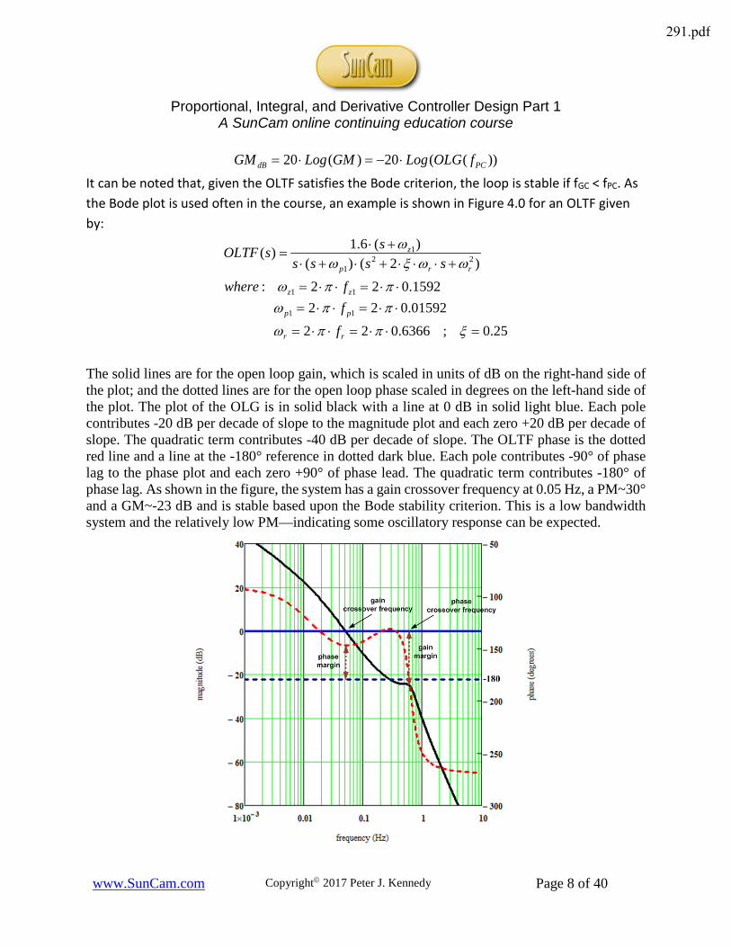
It can be noted that, given the OLTF satisfies the Bode criterion, the loop is stable if fGC < fPC. As the Bode plot is used often in the course, an example is shown in Figure 4.0 for an OLTF given by:
25.0;6366.02201592.0221592.022:
)2()()(6.1)(
11
11
221
1
=⋅⋅=⋅⋅=
⋅⋅=⋅⋅=⋅⋅=⋅⋅=
+⋅⋅⋅+⋅+⋅+⋅
=
ξππω
ππωππω
ωωξωω
rr
pp
zz
rrp
z
fffwhere
ssssssOLTF
The solid lines are for the open loop gain, which is scaled in units of dB on the right-hand side of the plot; and the dotted lines are for the open loop phase scaled in degrees on the left-hand side of the plot. The plot of the OLG is in solid black with a line at 0 dB in solid light blue. Each pole contributes -20 dB per decade of slope to the magnitude plot and each zero +20 dB per decade of slope. The quadratic term contributes -40 dB per decade of slope. The OLTF phase is the dotted red line and a line at the -180° reference in dotted dark blue. Each pole contributes -90° of phase lag to the phase plot and each zero +90° of phase lead. The quadratic term contributes -180° of phase lag. As shown in the figure, the system has a gain crossover frequency at 0.05 Hz, a PM~30° and a GM~-23 dB and is stable based upon the Bode stability criterion. This is a low bandwidth system and the relatively low PM—indicating some oscillatory response can be expected.
291.pdf

Proportional, Integral, and Derivative Controller Design Part 1
A SunCam online continuing education course
www.SunCam.com Copyright 2017 Peter J. Kennedy Page 9 of 40
Figure 4.0 Example Bode Plot for Example
3.3 Time to Frequency Domain Conversion: Using the Laplace transform, the relationship between the time and frequency domain for a first and second order plant can be evaluated as shown in Table 4.0. For both plants, to shorten notation x(t) equals the plant input and y(t) the output. The table describes the differential equation, its frequency domain conversion and the plant and output response. For the 1st order plant the term τ is the plant time constant while KS is the scaling factor.
Table 4.0 1st and 2nd Order Time and Frequency Domain Representations 1st Order Plant 2nd Order Plant
time )()()( txKtyty S ⋅⋅=⋅+ ττ )()()(2)( 20
200 txKtytyty S ⋅⋅=⋅+⋅⋅⋅+ ωωωξ
frequency ( ) )()( sXKsYs S ⋅⋅=⋅+ ττ ( ) )()(2 20
200
2 sXKsYss S ⋅⋅=⋅+⋅⋅⋅+ ωωωξ
plant τ
τ+⋅
=s
KsP s)( 200
2
20
2)(
ωωξω
+⋅⋅⋅+⋅
=ss
KsP S
output Y(s) )()()( sX
sKsXsP s ⋅+⋅
=⋅=τ
τ )(2
)()( 200
2
20 sX
ssKsXsP S ⋅
+⋅⋅⋅+⋅
=⋅=ωωξ
ω
transform )())(();())(();())(();())(( 2 sYstyLsXtxLsYstyLsYtyL ⋅==⋅==
For the 2nd order system, ζ is the damping constant and ω0 the natural frequency of the plant. This general procedure can be applied to a differential equation of any order. 4.0 Key Feedback Loop Relationships: Each block in the feedback control loop block diagram, Figure 3.0, can be expressed in the frequency domain using the Laplace transform described in the last section, assuming all constraints are met. These relationships are common to all linear control loops including ones using a PID controller, discussed herein. In the frequency domain, blocks can be treated algebraically with each element of the loop in the block diagram treated as a frequency dependent function. Referring to the block diagram of Figure 3.0, an expression for the control signal, denoted as u(s) and the output can be obtained algebraically as:
)()(; sPIDsCn(s))(e(s)C(s)then: u(s)output(s)H(s)in(s)cmd as:e(s)ervo errordefining s
output(s))H(s)(n(s)in(s)(cmdC(s)s)Control:u(
=−⋅=⋅−=
⋅+−⋅=
The output is then given as:
)))(()()(()()(,)))()(()()(()()]()([)()(
snoutput(s)H(s)in(s)cmdsCsdsPsoutputorsnsesCsdsPsusdsPsoutput−⋅−⋅+⋅=
−⋅+⋅=+⋅=
291.pdf

Proportional, Integral, and Derivative Controller Design Part 1
A SunCam online continuing education course
www.SunCam.com Copyright 2017 Peter J. Kennedy Page 10 of 40
Solving for the output:
)()()()(1
)()()()()()(1
)(
)()()()(1
)()()(
snsHsCsP
sCsPsdsHsCsP
sP
sincmdsHsCsP
sCsPsoutput
⋅
⋅⋅+
⋅−⋅
⋅⋅+
+⋅
⋅⋅+
⋅=
The first term in brackets describes the response from the command input to the output and is termed the closed loop transfer function (CLTF), with a magnitude called the closed loop gain (CLG) or:
⋅⋅+
⋅=
⋅⋅+
⋅=
)()()(1)()()(;
)()()(1)()()(
sHsCsPsCsPsCLG
sHsCsPsCsPsCLTF
The control compensator gain, |C(s)|, is normally very high and the primary gain term such that magnitude of the product of the three terms |P(s)*C(s)*H(s)|>> 1 over the effective operating bandwidth of the loop. This product is the open loop transfer function (OLTF) and its magnitude called the open loop gain (OLG):
)()()()(;)()()()( sHsCsPsOLGsHsCsPsOLTF ⋅⋅=⋅⋅= The feedback term is often a unity gain (or scaled to provide unity gain in the feedback path) as it is simply sensing the plant output. This being the case, the closed loop gain, CLG is unity over the operating bandwidth of the loop and rolls off towards zero at high frequency. If the feedback gain is not unity, it will change the closed loop gain from one to the inverse of the feedback gain magnitude (i.e. 1/H). The second expression accounts for the impact of disturbances on the response. The transfer function in brackets multiplying the disturbance is often termed the compliance—as in how compliant the loop is to a disturbance.
⋅⋅+
=)()()(1
)()(sHsCsP
sPsCompliance
This term attenuates the disturbance, primarily due to the high gain control term (C(s) = PID(s)) in the open loop gain. Therefore, the higher the controller gain, the more disturbance rejection and the less impact the disturbances will have on the output. However, this gain will be limited by the stability of the loop. Finally, as modeled, the last term is sensor noise which, as shown effectively, adds directly to the output since it is multiplied by the closed loop gain. As it is basically input to the same summing junction as the command input, this would be expected. The servo error between the command input and the output is given by:
)()()()(1
)()()()()()(1
)(
)()()()(1))(1)(()(1)()()(
snsHsCsP
sCsPsdsHsCsP
sP
sincmdsHsCsPsHsCsPsoutputsincmdse
⋅
⋅⋅+
⋅+⋅
⋅⋅+
−⋅
⋅⋅+−⋅−
=−=
The error is effectively the accuracy with which the output follows the command input. The first term in brackets that is multiplying the command input is often called the loop sensitivity function.
291.pdf
Proportional, Integral, and Derivative Controller Design Part 1
A SunCam online continuing education course
www.SunCam.com Copyright 2017 Peter J. Kennedy Page 11 of 40
For unity feedback (H(s)~1) this term is effectively one over the open loop gain—similar to the compliance function discussed previously, or:
1)()()(1
1)( =
⋅+
= sHforsCsP
sySensitivit
The transfer function for the plant can vary significantly based upon the application. As will be discussed, the PID works best with simpler first and second order plants. For process control applications, delays or dead time must often be accounted for and a simple three parameter plant model can sometimes be used to describe its response as:
timedelayordeadLtconstimeresponseTscalingprocessK
eTs
KsP sL
−−−
⋅⋅+
= −
;tan;
)1
()(
Compensation for the delay is not always possible with a simple controller. If the delay is small relative to the sampling period, a simple first order Taylor Series (e-sL ≈ [1-sL]) or Pade’ approximation (e-sL ≈ [1-sL]/[1+sL]) may be sufficient. However, if the delay is significant relative to the sampling period, the PID would need to be combined with a more advanced control algorithm such as the Smith Predictor [1, 2] discussed in part 2 of this course. The error will be a function of the attenuation provided by this term as well as the magnitude of the command, disturbance, and noise. One final error relationship of importance is the steady state error which is defined as:
[ ]
⋅
⋅+
⋅=⋅= →→ )()()(1
lim)(lim 00 sincmdsCsP
ssese ssSS
It is a measure of the error response or effectively the accuracy of a stable system as time goes to infinity. It is normally evaluated against three standard input signals: a step, ramp or rate, and parabolic input or acceleration. These signals have the Laplace transforms:
32 ;;s
Kparobolic
sK
ramps
Kstep parobolicrampstep →→→
The steady state error is often used as part of the control loop performance specification. The required response to these input signals will determine what is termed the loop ‘Type’; which refers to the open loop poles at s=0 or the number of integrators (i.e. 1/s terms) in the OLTF(s). If we describe a general input to the system as Kx/sn –which can be any of the above inputs depending on the value of n—then the steady state error can be written as:
[ ]
⋅⋅+
=
⋅
⋅+
⋅=⋅= −−→→→ )()(lim
)()(1lim)(lim 11000 sCsPss
KsK
sCsPssErrorsE nn
xsn
xssSS
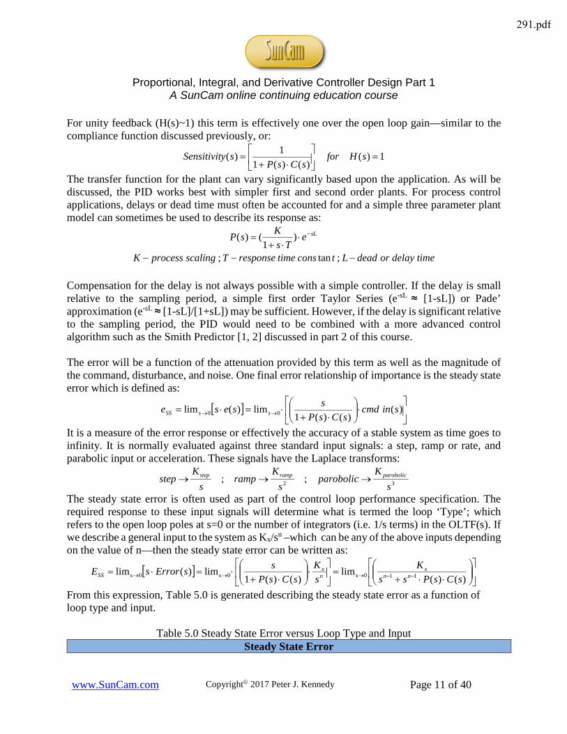
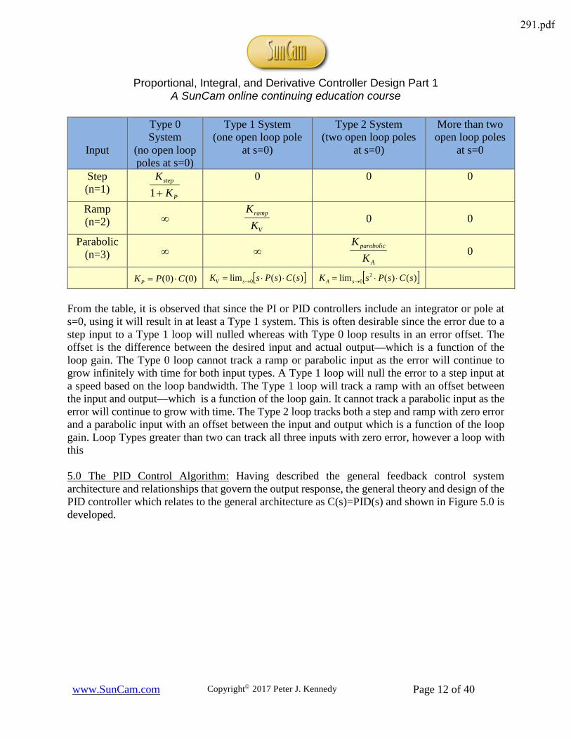
From this expression, Table 5.0 is generated describing the steady state error as a function of loop type and input.
Table 5.0 Steady State Error versus Loop Type and Input Steady State Error
291.pdf
Proportional, Integral, and Derivative Controller Design Part 1
A SunCam online continuing education course
www.SunCam.com Copyright 2017 Peter J. Kennedy Page 12 of 40
Input
Type 0 System
(no open loop poles at s=0)
Type 1 System (one open loop pole
at s=0)
Type 2 System (two open loop poles
at s=0)
More than two open loop poles
at s=0
Step (n=1)
P
step
KK+1
0 0 0
Ramp (n=2) ∞
V
ramp
KK
0 0
Parabolic (n=3) ∞ ∞
A
parobolic
KK
0
)0()0( CPKP ⋅= [ ])()(lim 0 sCsPsK sV ⋅⋅= → [ ])()(lim 20 sCsPsK sA ⋅⋅= →
From the table, it is observed that since the PI or PID controllers include an integrator or pole at s=0, using it will result in at least a Type 1 system. This is often desirable since the error due to a step input to a Type 1 loop will nulled whereas with Type 0 loop results in an error offset. The offset is the difference between the desired input and actual output—which is a function of the loop gain. The Type 0 loop cannot track a ramp or parabolic input as the error will continue to grow infinitely with time for both input types. A Type 1 loop will null the error to a step input at a speed based on the loop bandwidth. The Type 1 loop will track a ramp with an offset between the input and output—which is a function of the loop gain. It cannot track a parabolic input as the error will continue to grow with time. The Type 2 loop tracks both a step and ramp with zero error and a parabolic input with an offset between the input and output which is a function of the loop gain. Loop Types greater than two can track all three inputs with zero error, however a loop with this 5.0 The PID Control Algorithm: Having described the general feedback control system architecture and relationships that govern the output response, the general theory and design of the PID controller which relates to the general architecture as C(s)=PID(s) and shown in Figure 5.0 is developed.
291.pdf

Proportional, Integral, and Derivative Controller Design Part 1
A SunCam online continuing education course
www.SunCam.com Copyright 2017 Peter J. Kennedy Page 13 of 40
Figure 5.0 Feedback Control Loop with PID Controller
The PID controller structure, parameterized in terms of gain and referenced frequently in the literature, is:
)()()()(0
teKdeKteKtu D
t
IP ⋅+⋅+⋅= ∫ ττ
The control signal variable ‘u(t)’ was defined section 4.0 with the controller being the sum of three terms:
• A term proportional to the error with gain KP • A term proportional to the integral of the error with gain KI • A term proportional to the derivative of the error with gain KD
The time domain representation, parameterized in terms of gain, can be converted to the frequency domain using the Laplace Transform relationships defined in section 3, as:
)()()( sesKs
KKsu DI
P ⋅⋅++=
There are several versions of the controller that do not include all three terms; proportional plus integral (PI), proportional plus derivative (PD) or have a slightly different structure such as proportional plus integral and proportional plus derivative (PIPD). The controller’s versatility can be observed from the impact it has on key closed loop system time response characteristics that include:
• Rise Time: time required for the plant output to reach 90% of the desired level for the first time
• Overshoot: amount the peak level exceeds the steady state value; normalized to this value • Settling Time: time required for system to reach the steady state
291.pdf
Proportional, Integral, and Derivative Controller Design Part 1
A SunCam online continuing education course
www.SunCam.com Copyright 2017 Peter J. Kennedy Page 14 of 40
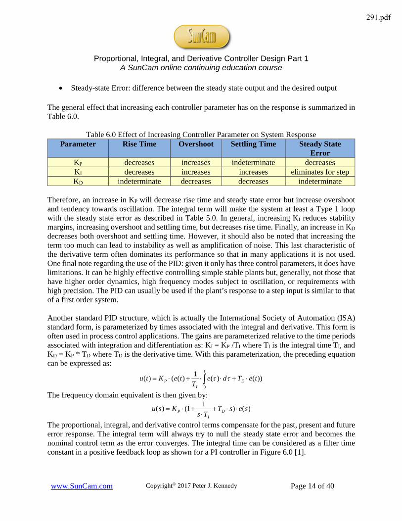
• Steady-state Error: difference between the steady state output and the desired output The general effect that increasing each controller parameter has on the response is summarized in Table 6.0.
Table 6.0 Effect of Increasing Controller Parameter on System Response Parameter Rise Time Overshoot Settling Time Steady State
Error KP decreases increases indeterminate decreases KI decreases increases increases eliminates for step KD indeterminate decreases decreases indeterminate
Therefore, an increase in KP will decrease rise time and steady state error but increase overshoot and tendency towards oscillation. The integral term will make the system at least a Type 1 loop with the steady state error as described in Table 5.0. In general, increasing KI reduces stability margins, increasing overshoot and settling time, but decreases rise time. Finally, an increase in KD decreases both overshoot and settling time. However, it should also be noted that increasing the term too much can lead to instability as well as amplification of noise. This last characteristic of the derivative term often dominates its performance so that in many applications it is not used. One final note regarding the use of the PID: given it only has three control parameters, it does have limitations. It can be highly effective controlling simple stable plants but, generally, not those that have higher order dynamics, high frequency modes subject to oscillation, or requirements with high precision. The PID can usually be used if the plant’s response to a step input is similar to that of a first order system. Another standard PID structure, which is actually the International Society of Automation (ISA) standard form, is parameterized by times associated with the integral and derivative. This form is often used in process control applications. The gains are parameterized relative to the time periods associated with integration and differentiation as: KI = KP /TI where TI is the integral time TI, and KD = KP * TD where TD is the derivative time. With this parameterization, the preceding equation can be expressed as:
))()(1)(()(0
teTdeT
teKtu D
t
IP ⋅+⋅⋅+⋅= ∫ ττ
The frequency domain equivalent is then given by:
)()11()( sesTTs
Ksu DI
P ⋅⋅+⋅
+⋅=
The proportional, integral, and derivative control terms compensate for the past, present and future error response. The integral term will always try to null the steady state error and becomes the nominal control term as the error converges. The integral time can be considered as a filter time constant in a positive feedback loop as shown for a PI controller in Figure 6.0 [1].
291.pdf

Proportional, Integral, and Derivative Controller Design Part 1
A SunCam online continuing education course
www.SunCam.com Copyright 2017 Peter J. Kennedy Page 15 of 40
Figure 6.0 PI Controller Configured as Positive Feedback through a Filter
The control signal is given by:
sTsusIsIseKsuI
P ⋅+=+⋅=
1)()(with)()()(
Solving these equations for I(s) results in the PI control signal:
)()()().()( sesT
KseKsusesT
KsII
PP
I
P ⋅⋅
+⋅=∴⋅⋅
=
The derivative term can provide a phase lead of up to ~50° and be considered as a predictive element can be seen from its definition:
)()()()()(lim)( 0 teTteTteT
teTtete DDD
DTD
⋅+≈+∴−+
= →
Issues with this term are that it amplifies noise, especially at high frequency and if it is too large—which can lead to oscillation and instability in a PID controller. Noise can be attenuated by adding a pole to roll-off the frequency response or effectively filter the signal at high frequency. Effectively this is the implementation of the derivative term as a high pass filter. The structure with the roll off frequency is:
rolloff
DI
P
fawhere
seassaT
TsKsu
⋅⋅=
⋅+⋅
⋅+⋅
+⋅=
π2
)()11()(
5.1 Time versus Frequency Domain Representations: The two representations provide different perspectives of the controller. In the time domain, the controller consists of integral, proportional, and derivative parts corresponding to control terms that compensate for the past, present and future error response; each weighted by their respective gains. Intuitively this seems a reasonable approach, providing three states of the error dynamics to use for loop response compensation. In the frequency domain, terms cannot be treated separately and the benefits are not quite as obvious as in time domain. Without the derivative term, the PI controller frequency response can easily be interpreted with the representation:
)11()()(I
P TsKsPIsC
⋅+⋅==
In the frequency domain, this controller consists of a pole at 0 and a zero at 1/TI. In the time domain, this zero will normally cause an overshoot in the system step response dependent upon
291.pdf
Proportional, Integral, and Derivative Controller Design Part 1
A SunCam online continuing education course
www.SunCam.com Copyright 2017 Peter J. Kennedy Page 16 of 40
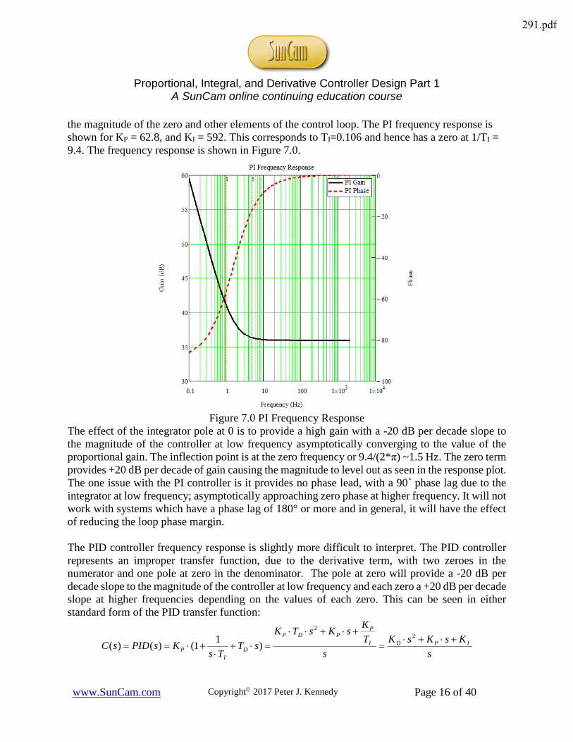
the magnitude of the zero and other elements of the control loop. The PI frequency response is shown for KP = 62.8, and KI = 592. This corresponds to TI=0.106 and hence has a zero at 1/TI = 9.4. The frequency response is shown in Figure 7.0.
Figure 7.0 PI Frequency Response
The effect of the integrator pole at 0 is to provide a high gain with a -20 dB per decade slope to the magnitude of the controller at low frequency asymptotically converging to the value of the proportional gain. The inflection point is at the zero frequency or 9.4/(2*π) ~1.5 Hz. The zero term provides +20 dB per decade of gain causing the magnitude to level out as seen in the response plot. The one issue with the PI controller is it provides no phase lead, with a 90˚ phase lag due to the integrator at low frequency; asymptotically approaching zero phase at higher frequency. It will not work with systems which have a phase lag of 180° or more and in general, it will have the effect of reducing the loop phase margin. The PID controller frequency response is slightly more difficult to interpret. The PID controller represents an improper transfer function, due to the derivative term, with two zeroes in the numerator and one pole at zero in the denominator. The pole at zero will provide a -20 dB per decade slope to the magnitude of the controller at low frequency and each zero a +20 dB per decade slope at higher frequencies depending on the values of each zero. This can be seen in either standard form of the PID transfer function:
sKsKsK
sTKsKsTK
sTTs
KsPIDsC IPDI
PPDP
DI
P+⋅+⋅
=+⋅+⋅⋅
=⋅+⋅
+⋅==2
2
)11()()(
291.pdf

Proportional, Integral, and Derivative Controller Design Part 1
A SunCam online continuing education course
www.SunCam.com Copyright 2017 Peter J. Kennedy Page 17 of 40
The magnitude |*|, phase Φ, and zeroes of both forms of the PID transfer function are given in Table 7.0.
Table 7.0 PID Standard Form Magnitude, Phase, Zeroes Standard PID Gain Standard PID Time
)( ωjPID ( ))(2
ωω⋅−
− DIP
KKjK ( ))11(
2
ωω
⋅⋅⋅−
−⋅I
DIP T
TTjK
)( ωjPID ( ) 222
⋅−+
ωωDI
PKKK ( ) 2211
⋅
⋅⋅−+⋅
ωω
I
DIP T
TTK
( ))( ωjPIDΦ ( )
⋅⋅−
−ωω
P
DI
KKKa
2
tan ( )
⋅
⋅⋅−−
ωω
I
DI
TTTa
21tan
Zeroes 21, ZZ ss
⋅−
⋅− 2411
2 P
ID
D
P
KKK
KK
−
⋅−
I
D
D TT
T411
21
It can be observed that if TD/TI > ¼ (or KD*KI / KP
2 > 1/4) the zeroes are complex roots. The zeroes of the plant and compensator will also be the zeroes of the closed loop system. For a pair of zeroes, the PID(s) frequency response magnitude will dip or notch at ~ωmin = √(KI/KD) = √(1/(TI*TD)). As an example, the PID frequency response is shown for KP =62.8, KI = 592, and KD =10. This corresponds to TI =0.106 and TD =0.16 so TD / TI = 1.5 and the zeroes are complex -3.1±7j. The controller frequency response is shown in Figure 8.0 with a notch at ~1.22 Hz.
Figure 8.0 PID Frequency Response
291.pdf
Proportional, Integral, and Derivative Controller Design Part 1
A SunCam online continuing education course
www.SunCam.com Copyright 2017 Peter J. Kennedy Page 18 of 40
The overall response with the derivative is dominated by this term at high frequencies, the gain increasing at + 20 dB per decade. This characteristic is one issue with a simple implementation of the controller and the reason it is normally implemented as a high pass filter with a pole to roll off the response at high frequency as opposed to the +20 dB per decade slope. Of course, the overall benefit of the PID will depend on the characteristic of the process itself. If it is already low frequency or heavily filtered, the roll-off may not be required. In general, however, it is good practice since the derivative will always differentiate noise amplifying it especially at high frequency. 5.2 Closed Loop System Simulation with a PID Controller: To provide a visualization of the effect each PID term has on the closed loop response, an example based upon the block diagram in Figure 2.0 is provided with the terms defined as:
Hzffaedisturbancandnoise
sFassaK
sKKsC
Hzffss
fsP
rolloffrolloff
DI
P
PP
P
250;20
1)(
)()(
1;)2(
2)(
=⋅⋅==
=+⋅
⋅++=
=⋅⋅+⋅
⋅⋅=
π
ππ
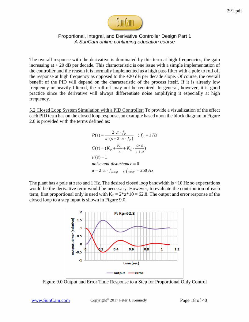
The plant has a pole at zero and 1 Hz. The desired closed loop bandwidth is ~10 Hz so expectations would be the derivative term would be necessary. However, to evaluate the contribution of each term, first proportional only is used with KP = 2*π*10 = 62.8. The output and error response of the closed loop to a step input is shown in Figure 9.0.
Figure 9.0 Output and Error Time Response to a Step for Proportional Only Control
291.pdf
Proportional, Integral, and Derivative Controller Design Part 1
A SunCam online continuing education course
www.SunCam.com Copyright 2017 Peter J. Kennedy Page 19 of 40
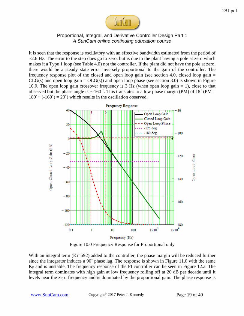
It is seen that the response is oscillatory with an effective bandwidth estimated from the period of ~2.6 Hz. The error to the step does go to zero, but is due to the plant having a pole at zero which makes it a Type 1 loop (see Table 4.0) not the controller. If the plant did not have the pole at zero, there would be a steady state error inversely proportional to the gain of the controller. The frequency response plot of the closed and open loop gain (see section 4.0, closed loop gain = CLG(s) and open loop gain = OLG(s)) and open loop phase (see section 3.0) is shown in Figure 10.0. The open loop gain crossover frequency is 3 Hz (when open loop gain = 1), close to that observed but the phase angle is ~-160 ˚. This translates to a low phase margin (PM) of 18˚ (PM = 180˚+ (-160˚) = 20˚) which results in the oscillation observed.
Figure 10.0 Frequency Response for Proportional only
With an integral term (Ki=592) added to the controller, the phase margin will be reduced further since the integrator induces a 90˚ phase lag. The response is shown in Figure 11.0 with the same KP and is unstable. The frequency response of the PI controller can be seen in Figure 12.a. The integral term dominates with high gain at low frequency rolling off at 20 dB per decade until it levels near the zero frequency and is dominated by the proportional gain. The phase response is
291.pdf

Proportional, Integral, and Derivative Controller Design Part 1
A SunCam online continuing education course
www.SunCam.com Copyright 2017 Peter J. Kennedy Page 20 of 40
also shown, adding 90˚ of lag at low frequency that causes the instability. The system frequency response is shown in Figure 12.b. The open loop gain crossover frequency is still at 3 Hz but the phase is never greater than -180˚resulting in system instability
Figure 11.0 Output and Error Time Response to a Step for PI Control
Figure 12.a PI Controller Frequency Response Figure 12.b System Frequency Response
The contribution of the integral term increases with decreasing integral time, however, this also reduces stability margins. Decreasing Ki is effectively an increase in integral time. Reducing both PI control gains, Kp and Ki , will stabilize the loop, but this also results in a lower bandwidth or slower response time. With the Kp and Ki gains reduced, the resulting time response shown in Figure 13.0 and the system frequency response in Figure 14.b. The gain crossover frequency is
291.pdf
Proportional, Integral, and Derivative Controller Design Part 1
A SunCam online continuing education course
www.SunCam.com Copyright 2017 Peter J. Kennedy Page 21 of 40
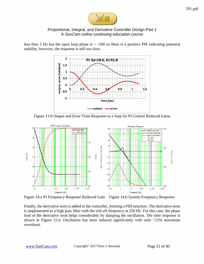
less than 2 Hz but the open loop phase is ~ -160 so there is a positive PM indicating potential stability, however, the response is still too slow.
Figure 13.0 Output and Error Time Response to a Step for PI Control Reduced Gains
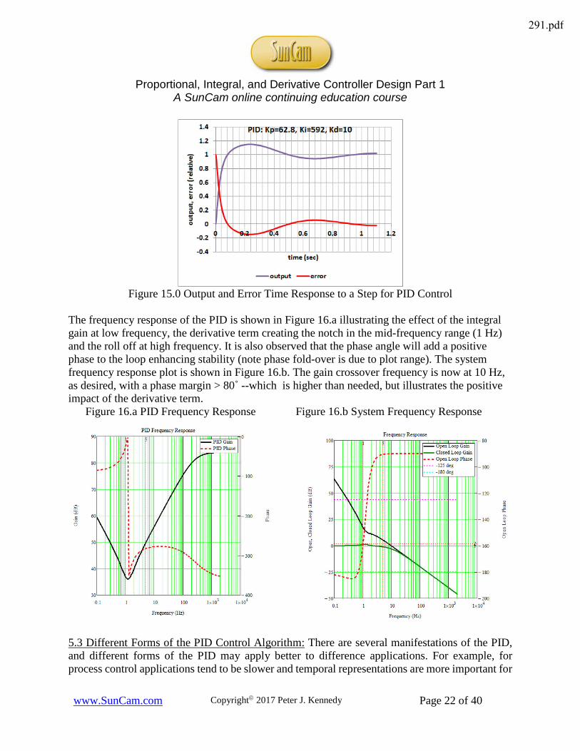
Figure 14.a PI Frequency Response Reduced Gain Figure 14.b System Frequency Response Finally, the derivative term is added to the controller, forming a PID structure. The derivative term is implemented as a high pass filter with the roll-off frequency at 250 Hz. For this case, the phase lead of the derivative term helps considerably by damping the oscillation. The time response is shown in Figure 15.0. Oscillation has been reduced significantly with only ~15% maximum overshoot.
291.pdf
Proportional, Integral, and Derivative Controller Design Part 1
A SunCam online continuing education course
www.SunCam.com Copyright 2017 Peter J. Kennedy Page 22 of 40
Figure 15.0 Output and Error Time Response to a Step for PID Control
The frequency response of the PID is shown in Figure 16.a illustrating the effect of the integral gain at low frequency, the derivative term creating the notch in the mid-frequency range (1 Hz) and the roll off at high frequency. It is also observed that the phase angle will add a positive phase to the loop enhancing stability (note phase fold-over is due to plot range). The system frequency response plot is shown in Figure 16.b. The gain crossover frequency is now at 10 Hz, as desired, with a phase margin > 80˚ --which is higher than needed, but illustrates the positive impact of the derivative term. Figure 16.a PID Frequency Response Figure 16.b System Frequency Response
5.3 Different Forms of the PID Control Algorithm: There are several manifestations of the PID, and different forms of the PID may apply better to difference applications. For example, for process control applications tend to be slower and temporal representations are more important for
291.pdf

Proportional, Integral, and Derivative Controller Design Part 1
A SunCam online continuing education course
www.SunCam.com Copyright 2017 Peter J. Kennedy Page 23 of 40
tuning performance. A higher bandwidth target tracking application design may rely more on placement and tuning for a desired frequency response so that frequency parameters are more relevant. There are two standard PID algorithm representations as discussed previously. One is parameterized in terms of a gain, integral time, and derivative time as:
)()11()( sesTTs
Ksu DI
P ⋅⋅+⋅
+⋅=
or replacing the derivative with a high pass filter:
)()11()( seassaT
TsKsu D
IP ⋅
+⋅
⋅+⋅
+⋅=
The other standard form is parameterized in terms of absolute gain as:
)()()( sesKs
KKsu DI
P ⋅⋅++=
Again, the derivative can be replaced with a high pass filter as:
)()()( seassaK
sKKsu D
IP ⋅
+⋅
⋅++=
With the two standard-forms, the proportional gains are equivalent and the other gains related as: KI = KP /TI where TI is the integral time TI, and KD = KP * TD where TD is the derivative time. In the latter representation, the parameter values are related to absolute gains rather than times associated with integration and the derivative. As the parameters linearly weight the operator of each term, it is useful in analytical calculations; it also has the advantage that it is possible to obtain pure proportional, integral, or derivative action by finite values of the parameters. A slightly different version of the controller is the forward path product of a proportional integral cascaded with a proportional derivative controller (PI*PD) as given by:
)()1()1()()1()11()( seTs
sTsTKsesTTs
KsuI
DIPD
IP ⋅
⋅⋅′+⋅⋅′+
⋅′=⋅⋅′+⋅′⋅
+⋅′=
This version is much easier to work with in the frequency domain as terms are factored so that both zeroes, the pole at zero, and DC gain are easily delineated. One interpretation of this form is a PI controller operating on the predicted value the error signal. The parameterization of this structure and the standard structure are not equivalent. The factored form can be equated to the standard form by multiplying out the factors and equating like coefficients:
DI
IDDII
I
DIPP TT
TTTTTTT
TTKK′+′′⋅′
=′+′=′′+′
⋅′= ;;)(
Equating the standard form to a factored form is possible only if the zeroes of the standard form are real—which requires TI>4*TD. The factored form can also use the high pass filter for noise attenuation as previously discussed, or:
)()1()11()( seassaT
TsKsu D
IP ⋅
+⋅
⋅′+⋅′⋅
+⋅′=
In this manifestation, the PD term can also be interpreted as a lead compensator. Expanding this term results in:
291.pdf
Proportional, Integral, and Derivative Controller Design Part 1
A SunCam online continuing education course
www.SunCam.com Copyright 2017 Peter J. Kennedy Page 24 of 40
( ) )(1)11(1)( seas
Taas
TsTaKsu D
IDP ⋅
+′⋅+
+⋅
′⋅+⋅′⋅+⋅′=
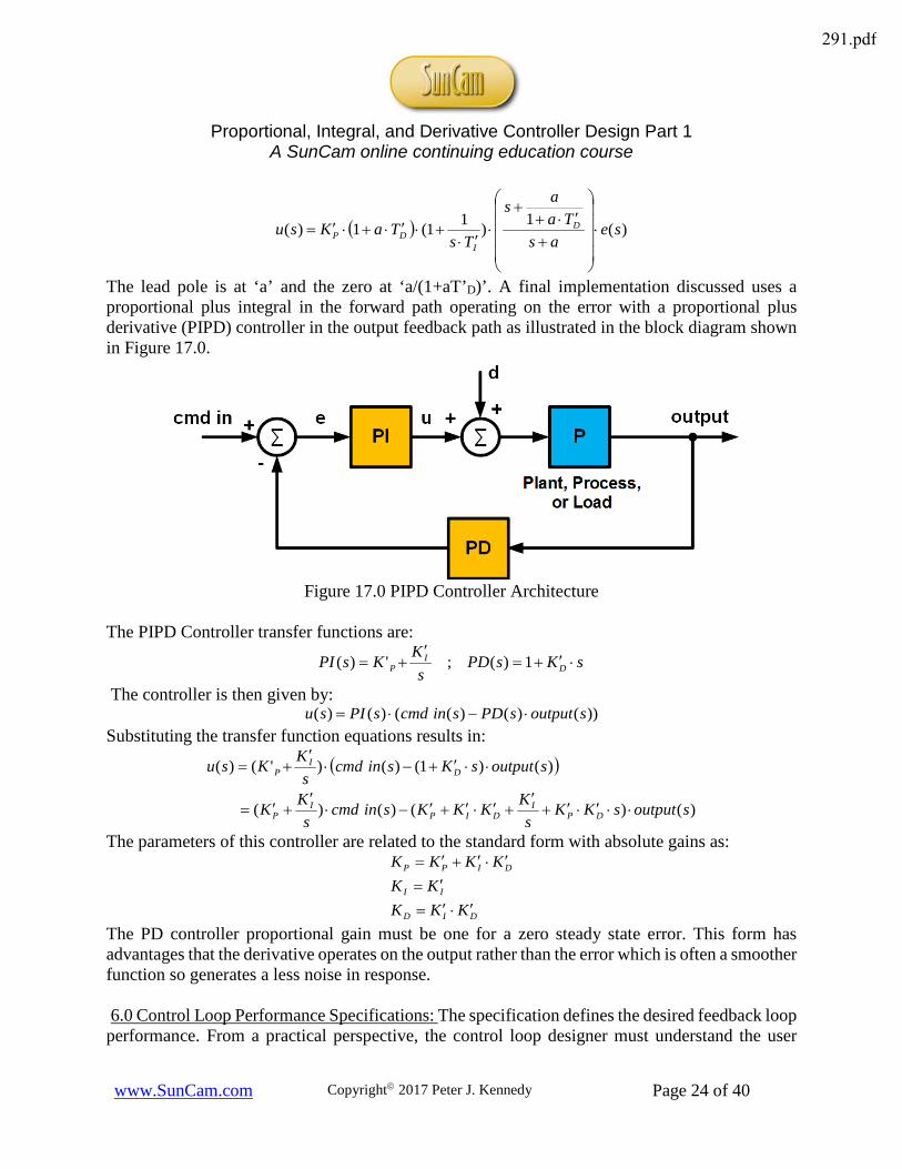
The lead pole is at ‘a’ and the zero at ‘a/(1+aT’D)’. A final implementation discussed uses a proportional plus integral in the forward path operating on the error with a proportional plus derivative (PIPD) controller in the output feedback path as illustrated in the block diagram shown in Figure 17.0.
Figure 17.0 PIPD Controller Architecture
The PIPD Controller transfer functions are:
sKsPDs
KKsPI DI
P ⋅′+=′
+= 1)(;')(
The controller is then given by: ))()()(()()( soutputsPDsincmdsPIsu ⋅−⋅=
Substituting the transfer function equations results in:
( )
)()()()(
)()1()()'()(
soutputsKKs
KKKKsincmds
KK
soutputsKsincmds
KKsu
DPI
DIPI
P
DI
P
⋅⋅′⋅′+′
+′⋅′+′−⋅′
+′=
⋅⋅′+−⋅′
+=
The parameters of this controller are related to the standard form with absolute gains as:
DID
II
DIPP
KKKKK
KKKK
′⋅′=
′=
′⋅′+′=
The PD controller proportional gain must be one for a zero steady state error. This form has advantages that the derivative operates on the output rather than the error which is often a smoother function so generates a less noise in response. 6.0 Control Loop Performance Specifications: The specification defines the desired feedback loop performance. From a practical perspective, the control loop designer must understand the user
291.pdf

Proportional, Integral, and Derivative Controller Design Part 1
A SunCam online continuing education course
www.SunCam.com Copyright 2017 Peter J. Kennedy Page 25 of 40
requirements to develop a satisfactory specification. Key characteristics often specified by a user are accuracy and response time for a defined command signal or range of signals and the disturbance and noise environment. From this information, the designer must develop the control requirements and specification. As discussed previously, accuracy and disturbance rejection are improved by a high gain controller, as is response time. As gain is effectively proportional to bandwidth, this implies a higher bandwidth improves performance. However, as the bandwidth increases, the loop stability margins begin to decrease, more overshoot results, control elements can saturate, and the noise between loop elements can be amplified. So, the design is a tradeoff between the user requirements and control loop specifications that meet these requirements with sufficient stability margins. Control specific specifications can be defined in either the time or frequency domain and need to be derived from system performance specifications. In the time domain they may relate directly, as discussed in section 5.0, with response specified in terms of: rise time, overshoot, settling time, and steady state error—all of which are a function of bandwidth and the control compensator structure. In the frequency domain, they are often derived from disturbance rejection and maximum allowable servo error requirements; as they relate to system performance. To achieve this performance the designer can specify the resonant peak, peak frequency, gain crossover frequency, bandwidth (which in some cases are directly related), and the minimum allowable phase and gain margins. The resonant peak is a maximum of the gain at the peak frequency. Another important specification is the control loop type which as discussed previously refers to the number of integrators within the loop; either due to the controller or the plant dynamics. The loop type or number of integrators will determine the accuracy (maximum error) with which the output follows an input command or rejects a disturbance in the long term. The integrator also provides very high gain at low frequency which is good for disturbance rejection and improved accuracy; however, each pole at s=0 also provides a -90° phase shift which can impact stability. The robustness of the controller design must also be considered. If the plant parameters change for whatever reason, what will happen to the loop stability margins? The controller design must account for these variations. This can be accomplished by designing for the worst-case plant variation and ensuring the system meets the stability margins over the full range of plant variation; measuring the plant response (i.e. plant identification) and changing control parameters to account for the plant changes (either manually or on a scheduled basis), or a using an adaptive controller that automatically adjusts the control parameters as a function of the plant variations. 7.0 PID Controller Design: Most general methods for control system design can be applied to PID control; within the constraints of the controller structure. PID controller design can be categorized as derived from manual tuning and measurement processes and/or those more analytically determined. A number of special methods made specifically for PID control have also been developed; often called tuning methods. Irrespective of the method, however, the design must
291.pdf

Proportional, Integral, and Derivative Controller Design Part 1
A SunCam online continuing education course
www.SunCam.com Copyright 2017 Peter J. Kennedy Page 26 of 40
always account for characteristics of the load disturbances, sensor noise, process uncertainty reference signal so that a robust design is achieved. 7.1 Manual Tuning Based on Process Measurements [1, 2]: The tuning algorithms developed by Ziegler and Nichols are among the most well-known methods referenced in literature. They are based on characterization of process dynamics by a few controller parameters and simple equations relating them to PID parameters. There are two baseline methods termed the step response and frequency response methods along with many subsequent modifications derived from these methods to improve performance 7.1.1 The Ziegler and Nichols Step Response Method [1, 2]: The step response method characterizes the measured open loop plant step response with two parameters, ‘a’ and ‘L’. This method is applicable to plants with a bounded step response; results being best when the response is close to being first order. The definitions of the parameters are shown in Figure 18 with the full step response to the left and the expanded region relevant to the design parameters ‘a’ and ‘L’ to the right.
Figure 18 Characterization of a Step Response in the Ziegler Nichols Step Response Method. The tangent to the step response slope at its maximum value is determined and a line is drawn intersecting the time and state response axes. The intersections with the coordinate axes provide the two parameters as shown in the figure. The time interval intersected on the time axis is termed ‘L’ and the state delta intersected on the state response axis ‘a’. The PID controller parameters are a function of these parameters as shown in Table 8.0 with Tp being an estimate of the closed loop period or response time.
Table 8.0 PID Controller Parameters for Ziegler Nichols Step Response Method Controller KP TI TD Tp
P 1/a 4L PI 0.9/a 3L 5.7L
PID 1.2/a 2L L/2 3.4L
291.pdf
Proportional, Integral, and Derivative Controller Design Part 1
A SunCam online continuing education course
www.SunCam.com Copyright 2017 Peter J. Kennedy Page 27 of 40
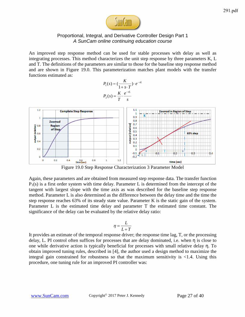
An improved step response method can be used for stable processes with delay as well as integrating processes. This method characterizes the unit step response by three parameters K, L and T. The definitions of the parameters are similar to those for the baseline step response method and are shown in Figure 19.0. This parameterization matches plant models with the transfer functions estimated as:
se
TKsP
eTs
KsP
sL
sL
−
−
⋅=
⋅⋅+
=
)(
)1
()(
2
1
Figure 19.0 Step Response Characterization 3 Parameter Model
Again, these parameters and are obtained from measured step response data. The transfer function P1(s) is a first order system with time delay. Parameter L is determined from the intercept of the tangent with largest slope with the time axis as was described for the baseline step response method. Parameter L is also determined as the difference between the delay time and the time the step response reaches 63% of its steady state value. Parameter K is the static gain of the system. Parameter L is the estimated time delay and parameter T the estimated time constant. The significance of the delay can be evaluated by the relative delay ratio:
TLL+
=η
It provides an estimate of the temporal response driver; the response time lag, T, or the processing delay, L. PI control often suffices for processes that are delay dominated, i.e. when η is close to one while derivative action is typically beneficial for processes with small relative delay η. To obtain improved tuning rules, described in [4], the author used a design method to maximize the integral gain constrained for robustness so that the maximum sensitivity is <1.4. Using this procedure, one tuning rule for an improved PI controller was:
291.pdf

Proportional, Integral, and Derivative Controller Design Part 1
A SunCam online continuing education course
www.SunCam.com Copyright 2017 Peter J. Kennedy Page 28 of 40
<⋅⋅<<⋅
⋅<=
<⋅⋅
⋅<⋅=
LTforLTLTforT
TLforLT
LTforK
TLforLK
TK
I
P
24.021.08.0
1.08
215.0
23.02
7.1.2 The Ziegler Nichols Frequency Response Method [1, 2]: A second method developed by Ziegler and Nichols is a simple characterization of the frequency response of the plant dynamics. The design is based on knowledge of the control loop frequency when plant’s phase is -180˚. On the Nyquist plot of the process transfer function P(s); this is the point where the Nyquist curve intersects the negative real axis. On a Bode Plot, it is equivalent to a phase crossover frequency for the open loop plant response; defining a boundary between a stable and unstable response. The Ziegler Nichols Frequency Response Method is characterized by two parameters, the frequency ω180 and the gain at that frequency K180 =|P(iω180)|. The parameters Ku =1/K180 and Tu = 2π / ω180, termed the ultimate gain and the ultimate period are used to derive the PID controller gains. These parameters are determined by connect a controller to the process; setting the parameters so that control action is proportional, i.e., TI =0 and TD= 0 and then increasing the gain slowly until the process oscillates. The gain at which this occurs is Ku and the oscillation period is Tu. The parameters of the controller are then given by Table 9.0. The frequency response method is an empirical tuning procedure where the controller parameters are obtained directly from process measurements combined with some simple rules. For a proportional controller, the rule is to simply increase the gain until the process oscillates and then reduce it by 50%.
Table 9.0 PID Controller Parameters for Ziegler Nichols frequency response method Controller K TI TD Tp
P 0.5Ku Tu PI 0.4Ku 0.8Tu 1.4Tu
PID 0.6Ku 0.5Tu 0.125Tu 0.85Tu An assessment [1] of the Ziegler Nichols Methods is that the tuning rules were developed to provide closed loop systems with good attenuation of load disturbances. The methods were based on extensive simulations. The design criterion was quarter amplitude decay ratio, which means that the amplitude of an oscillation should be reduced by a factor of four over a whole period. This corresponds to closed loop poles with a relative damping of about ξ = 0.2, which is too small. Controllers designed by the Ziegler Nichols rules inherently give closed loop systems with poor robustness. However, they are simple to use and do provide ball park estimates for the controller parameters with the final tuning done by trial and error. 7.2 Analytical Design Approaches: Analytical approaches (model matching criterion), again discussed in part 1, generally refer to i) trying to match the system response to that of a desired
291.pdf

Proportional, Integral, and Derivative Controller Design Part 1
A SunCam online continuing education course
www.SunCam.com Copyright 2017 Peter J. Kennedy Page 29 of 40
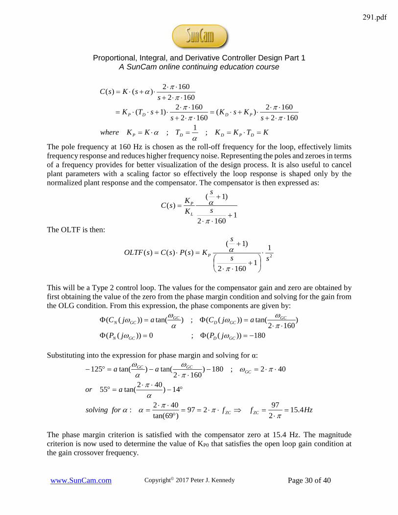
reference model or ii) signal or trying to place poles of the system response at those desired for a specified response. There are many control loop design techniques; most involve some form of loop shaping and/or algebraic pole-zero placement and cancellation. Loop shaping can be accomplished using Bode or Nyquist plot analysis. Visually, the Bode plot is easy to interpret and adjust the response especially if implemented in a mathematical computer aided design program (i.e. MatLab or MathCad). The Bode plot can be used with measured plant gain and phase response data, the plant-pole zero structure does not have to be known exactly (although the Bode design still subject minimum phase criterion). Algebraic methods appear straightforward but require knowledge of the plant pole-zero structure and care must be taken to insure stable design. For example, pole and zero cancellation must be done with some sensitivity analysis because they are never known exactly and in some cases, can change or drift. The is especially true if the poles and zeroes are not stable; direct cancellation can result in a pole/zero pair that are unstable (both roots in right half s-plane) as opposed cancellation of the unstable root. The loop Type can be adjusted using the PI or PID controller. When using any control term with a pure integrator, the output should be limited or other measures taken to insure windup of the integrator does not occur. A couple of simple design examples are provided. 7.2.1 Frequency Domain Design: Assume for a unity feedback loop the desired gain crossover frequency fGC = 40 Hz and the phase margin > 55°. This provides two criteria to satisfy with the compensator:
°−=Φ°=Φ+°=
=
125))((55))((180)2
1)()1
GC
GC
GC
fOLTForfOLTFPM
fOLG
From the definition of the open loop unity gain transfer function in section 3.0, this can be expressed as:
)(()(()(()((125))()(()2
2;1)()(
)()()1
GCDGCDGCNGCNGCGC
GCGCGCD
GCN
GCD
GCN
jPjCjPjCjPjC
fjPjP
jCjC
ωωωωωω
πωωω
ωω
Φ−Φ−Φ+Φ=°−=⋅Φ
⋅⋅==⋅
The plant is given by:
2)(sKsP L=
The plant parameter KL is the scaling factor. For a double integrator, the phase lag is -180° so it can be assumed to obtain the desired response a proportional plus derivative (PD) controller implemented with a roll-off filter or basically a lead compensator of the form:
291.pdf
Proportional, Integral, and Derivative Controller Design Part 1
A SunCam online continuing education course
www.SunCam.com Copyright 2017 Peter J. Kennedy Page 30 of 40
KTKKTKKwhere
sKsK
ssTK
ssKsC
DPDDP
PDDP
=⋅==⋅=
⋅⋅+⋅⋅
⋅+⋅=⋅⋅+
⋅⋅⋅+⋅⋅=
⋅⋅+⋅⋅
⋅+⋅=
;1;
16021602)(
16021602)1(
16021602)()(
αα
ππ
ππ
ππα
The pole frequency at 160 Hz is chosen as the roll-off frequency for the loop, effectively limits frequency response and reduces higher frequency noise. Representing the poles and zeroes in terms of a frequency provides for better visualization of the design process. It is also useful to cancel plant parameters with a scaling factor so effectively the loop response is shaped only by the normalized plant response and the compensator. The compensator is then expressed as:
11602
)1()(
+⋅⋅
+=
π
αs
s
KKsC
L
P
The OLTF is then:
21
11602
)1()()()(
ss
s
KsPsCsOLTF P ⋅
+
⋅⋅
+=⋅=
π
α
This will be a Type 2 control loop. The values for the compensator gain and zero are obtained by first obtaining the value of the zero from the phase margin condition and solving for the gain from the OLG condition. From this expression, the phase components are given by:
180))((;0))((
)1602
tan())((;)tan())((
−=Φ=Φ⋅⋅
=Φ=Φ
GCDGCN
GCGCD
GCGCN
jPjP
ajCajC
ωωπωω
αωω
Substituting into the expression for phase margin and solving for α:
Hzffforsolving
aor
aa
ZCZC
GCGCGC
4.15297297
)69tan(402:
14)402tan(55
402;180)1602
tan()tan(125
=⋅
=⇒⋅⋅==°
⋅⋅=
°−⋅⋅
=°
⋅⋅=−⋅⋅
−=°−
πππαα
απ
πωπω
αω
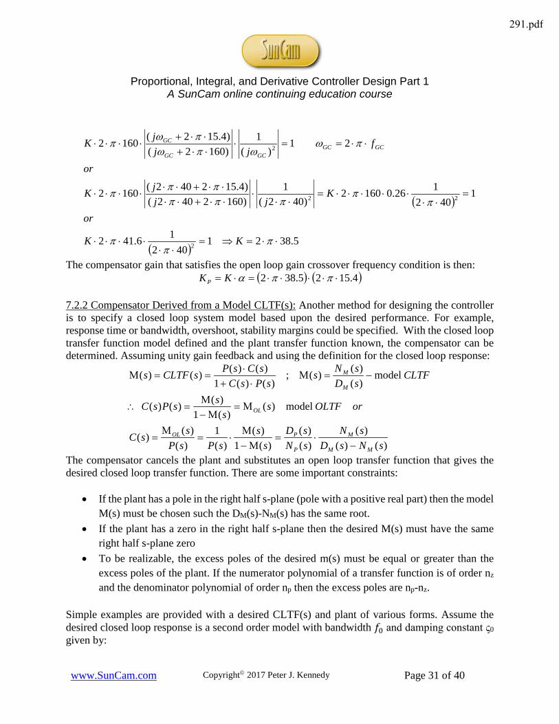
The phase margin criterion is satisfied with the compensator zero at 15.4 Hz. The magnitude criterion is now used to determine the value of KP0 that satisfies the open loop gain condition at the gain crossover frequency.
291.pdf
Proportional, Integral, and Derivative Controller Design Part 1
A SunCam online continuing education course
www.SunCam.com Copyright 2017 Peter J. Kennedy Page 31 of 40
( )
( )5.3821
40216.412
1402
126.01602)402(
1)1602402()4.152402(1602
21)(
1)1602()4.152(1602
2
22
2
⋅⋅=⇒=⋅⋅
⋅⋅⋅⋅
=⋅⋅
⋅⋅⋅⋅⋅=⋅⋅
⋅⋅⋅+⋅⋅⋅⋅+⋅⋅
⋅⋅⋅⋅
⋅⋅==⋅⋅⋅+⋅⋅+
⋅⋅⋅⋅
ππ
π
ππ
ππππππ
πωωπω
πωπ
KK
or
Kjj
jK
or
fjj
jK GCGCGCGC
GC
The compensator gain that satisfies the open loop gain crossover frequency condition is then: ( ) ( )4.1525.382 ⋅⋅⋅⋅⋅=⋅= ππαKKP
7.2.2 Compensator Derived from a Model CLTF(s): Another method for designing the controller is to specify a closed loop system model based upon the desired performance. For example, response time or bandwidth, overshoot, stability margins could be specified. With the closed loop transfer function model defined and the plant transfer function known, the compensator can be determined. Assuming unity gain feedback and using the definition for the closed loop response:
)()()(
)()(
)(1)(
)(1
)()()(
model)()(1
)()()(
model)()()(;
)()(1)()()()(
sNsDsN
sNsD
ss
sPsPssC
orOLTFss
ssPsC
CLTFsDsNs
sPsCsCsPsCLTFs
MM
M
P
POL
OL
M
M
−⋅=
Μ−Μ
⋅=Μ
=
Μ=Μ−
Μ=∴
−=Μ⋅+
⋅==Μ
The compensator cancels the plant and substitutes an open loop transfer function that gives the desired closed loop transfer function. There are some important constraints:
• If the plant has a pole in the right half s-plane (pole with a positive real part) then the model M(s) must be chosen such the DM(s)-NM(s) has the same root.
• If the plant has a zero in the right half s-plane then the desired M(s) must have the same right half s-plane zero
• To be realizable, the excess poles of the desired m(s) must be equal or greater than the excess poles of the plant. If the numerator polynomial of a transfer function is of order nz and the denominator polynomial of order np then the excess poles are np-nz.
Simple examples are provided with a desired CLTF(s) and plant of various forms. Assume the desired closed loop response is a second order model with bandwidth 𝑓𝑓0 and damping constant ς0 given by:
291.pdf

Proportional, Integral, and Derivative Controller Design Part 1
A SunCam online continuing education course
www.SunCam.com Copyright 2017 Peter J. Kennedy Page 32 of 40
( ) ( ) ( )
loopcontrolType1a2
ornattenuatioerrorloop2
1for
21;
11
222
22)(
2;2
)(
0
00
0
00
000
00
0
00
00
0
0
00
20
002000
2
20
ωζω
ωζωτ
ωζτ
τζω
ωζωζ
ζω
ωζω
πωωωζ
ω
⋅⋅≈←
⋅⋅≈Μ<<⋅
⋅⋅=
+⋅⋅⋅=
⋅⋅+⋅⋅
⋅⋅=
⋅⋅+⋅=Μ∴
⋅⋅=+⋅⋅⋅+
=Μ
PCs
sssssss
fss
s
OL
OL
Table 10.0 provides the controller that provides the desired closed loop response for a given plant transfer function. The plant parameters are defined as: frequencynaturalundampedplantω;constantdampingplantζ;fπ2ω mmmm −−⋅⋅=
Table 10.0 PID Controller for Desired Closed Loop Response and Plant Plant C(s) KP KI KD
22
2
2 mmm
mm
ssK
ωωζω
+⋅⋅⋅+⋅ ( )
++⋅
+ sKKsK
sI
PD11
0τ
mm
m
K ωζωζ⋅⋅
⋅
0
0 mK⋅⋅ 0
0
2 ζω
20
0
2 mmK ωζω
⋅⋅⋅
m
mm
sK
ωω
+⋅
( )
+⋅
+ sKK
sI
P11
0τ
mmK ωζω
⋅⋅⋅ 0
0
2
mK⋅⋅ 0
0
2 ζω
)( m
mm
ssK
ωω+⋅⋅
( ) ( )DP KsKs
⋅+⋅+1
10τ
mK⋅⋅ 0
0
2 ζω
mmK ωζω
⋅⋅⋅ 0
0
2
sKm ( )1
1
0 +sKP τ
mK⋅⋅ 0
0
2 ζω
7.3 Design Issues: To obtain good performance from a PID controller it is necessary to consider issues that impact or limit performance. A number of practical issues have been discussed. As mentioned, simple controllers like the PI and PID controller are not suitable for all processes. The PID controller is suitable for processes with almost monotone step responses, similar to that for a first order plant, provided that the requirements are not too stringent. A couple of issues mentioned previously were related to the integral and derivative terms, these and others are discussed in more detail in this section. The main issues, many of which are common to most controllers, are: Derivative Term: This issue has been described and can most easily be understood by simple differentiation of a sinusoid which results in the output being shifted by 90° and amplified by the radian frequency (2*π*f); the higher the frequency the greater the amplification. This is also obvious from the frequency response of the differentiator magnitude which goes to infinity as frequency increases. The implementation of the derivative as a high pass filter with a roll-off frequency that suppresses the high frequency noise reduces this problem. Effective noise can also be generated within the error signal due to disturbances or simply the functionality of the drive component. In section 5.3 ‘Different Forms of the PID Control Algorithm’, a structure using output feedback to implement the derivative terms was discussed that could mitigate any potential issue as the output is often a smoother function than the error so generates a less noise in the response.
291.pdf

Proportional, Integral, and Derivative Controller Design Part 1
A SunCam online continuing education course
www.SunCam.com Copyright 2017 Peter J. Kennedy Page 33 of 40
Integrator Windup: Use of an integrator in a physical system comes with the possibility integrator saturation. This effectively eliminates the integrator as a control term; converting a linear system response to a non-linear one. Windup results when the integral action saturates. All actuators have limits and for a control system with a wide range of operating conditions, the controller can reach these limits. The feedback loop is then broken and the system runs open loop because the actuator remains at its limit independent of the process output. If a controller with integrating action is used, the error will continue to be integrated. This means that the integral term may become very large or, in essence, “winds up”. It is then required that the error has opposite sign for a long period before things return to normal. The consequence is that any controller with integral action may give large transients when the actuator saturates. The simplest methods for addressing windup are limiting the integral term or input to the integral. However, this can also limit performance and generally does not really solve the problem. A better method is to measure the integrator output and as it approaches the actuator saturation level and provide feedback that reduces the input; sometimes termed the tracking and back calculation approach. A block diagram of the method is shown in Figure 20.0 [1].
Figure 20.0 Tracking and Back Calculation Wind-up Compensation Set Point Weighting [1]: With the standard PID control law, a step change in the reference signal results in an impulse to the control signal due to the derivative term. This problem can be avoided by filtering the reference value before being input to the controller or by using proportional only on part of the reference signal. This is called set point weighting. A PID controller given by:
( )
−⋅⋅⋅+⋅
⋅+−⋅⋅= )()(1)()()( soutputincmdsTse
TssoutputsincmdKsu D
IP σβ
291.pdf
Proportional, Integral, and Derivative Controller Design Part 1
A SunCam online continuing education course
www.SunCam.com Copyright 2017 Peter J. Kennedy Page 34 of 40
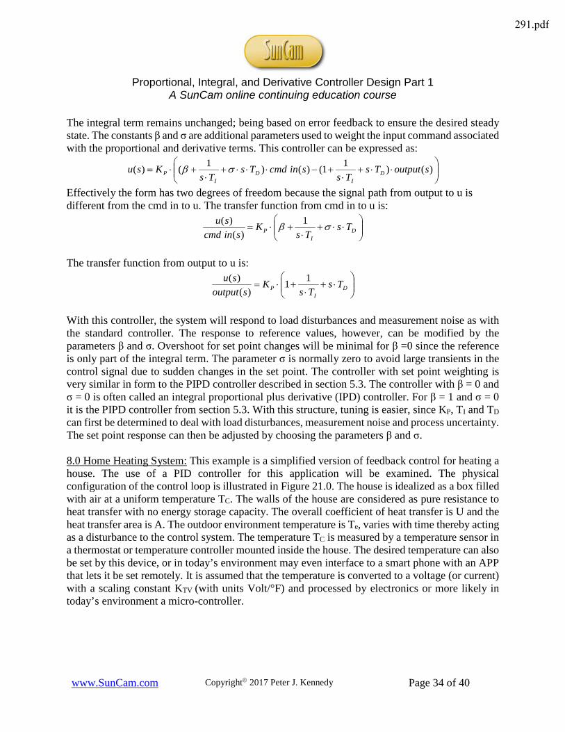
The integral term remains unchanged; being based on error feedback to ensure the desired steady state. The constants β and σ are additional parameters used to weight the input command associated with the proportional and derivative terms. This controller can be expressed as:
⋅⋅+
⋅+−⋅⋅⋅+
⋅+⋅= )()11()()1()( soutputTs
TssincmdTs
TsKsu D
ID
IP σβ
Effectively the form has two degrees of freedom because the signal path from output to u is different from the cmd in to u. The transfer function from cmd in to u is:
⋅⋅+
⋅+⋅= D
IP Ts
TsK
sincmdsu σβ 1
)()(
The transfer function from output to u is:
⋅+
⋅+⋅= D
IP Ts
TsK
soutputsu 11
)()(
With this controller, the system will respond to load disturbances and measurement noise as with the standard controller. The response to reference values, however, can be modified by the parameters β and σ. Overshoot for set point changes will be minimal for β =0 since the reference is only part of the integral term. The parameter σ is normally zero to avoid large transients in the control signal due to sudden changes in the set point. The controller with set point weighting is very similar in form to the PIPD controller described in section 5.3. The controller with β = 0 and σ = 0 is often called an integral proportional plus derivative (IPD) controller. For β = 1 and σ = 0 it is the PIPD controller from section 5.3. With this structure, tuning is easier, since KP, TI and TD can first be determined to deal with load disturbances, measurement noise and process uncertainty. The set point response can then be adjusted by choosing the parameters β and σ. 8.0 Home Heating System: This example is a simplified version of feedback control for heating a house. The use of a PID controller for this application will be examined. The physical configuration of the control loop is illustrated in Figure 21.0. The house is idealized as a box filled with air at a uniform temperature TC. The walls of the house are considered as pure resistance to heat transfer with no energy storage capacity. The overall coefficient of heat transfer is U and the heat transfer area is A. The outdoor environment temperature is Te, varies with time thereby acting as a disturbance to the control system. The temperature TC is measured by a temperature sensor in a thermostat or temperature controller mounted inside the house. The desired temperature can also be set by this device, or in today’s environment may even interface to a smart phone with an APP that lets it be set remotely. It is assumed that the temperature is converted to a voltage (or current) with a scaling constant KTV (with units Volt/°F) and processed by electronics or more likely in today’s environment a micro-controller.
291.pdf

Proportional, Integral, and Derivative Controller Design Part 1
A SunCam online continuing education course
www.SunCam.com Copyright 2017 Peter J. Kennedy Page 35 of 40
Figure 21.0 Concept Feedback Control Configuration for Heating a House
The controller will take the difference between the desired and actual temperature and generates a control signal to the furnace. This signal controls an actuator that increases or decreases the gas flow and effectively the amount of heat into the room. For this simple example, the actuation and heat generation are modeled as a linear process; in reality, it is a complex process. In developing a model of the system, it is assumed that initially the house is in equilibrium with constant values of TC and Te. The furnace will then be supplying sufficient heat to balance the heat loss to the environment. Any disturbance or change in the desired temperature will result in an increase or decrease in heat input from this original value. All variables should be considered deviations from their initial equilibrium condition. The simple first order thermal dynamic model for the heat balance in the house (the control loop plant) in the time domain is:
FBTUCM
FHrBTUAU
CM
Q
tTtTAUtQtTCMhousetheleavingenergythermalinenergythermalstoredenergythermal
P
P
M
eCMCP
°=⋅
°⋅=⋅
−−
−
−⋅⋅−=⋅⋅
−=
180;150assume
pressureconstantatairofheatspecifichouseinairofmass
hrBTUinenergythermalwhere
))()(()()(or
Converting to the frequency domain and rearranging terms:
291.pdf

Proportional, Integral, and Derivative Controller Design Part 1
A SunCam online continuing education course
www.SunCam.com Copyright 2017 Peter J. Kennedy Page 36 of 40
sec43202.1
1)(
)1()()(
==⋅⋅
=
+⋅+
+⋅⋅⋅=
HrAUCMwhere
ssT
sAUsQsT
P
eMC
τ
ττ
This represents the model of the plant; in terms of previous notation:
HrBTUF
ssAUsP
/)14320(1501
)1(1)( °
+⋅⋅=
+⋅⋅⋅=
τ
The temperature TC is then given by: ))()(()()( sTAUsQsPsT eMC ⋅⋅+⋅=
A feedback control system measures the house temperature TC and compares it to a desired temperature TS or the set point. The heat input is assumed proportional to this temperature difference, a simplification for the example. The control loop is shown in Figure 22.0. As the plant response is defined by a first order response, a reasonable choice for the controller, C(s), is a PID type implementation. The example will analyze the response for a P only and PI control.
Figure 22.0 Block diagram of home heating control servo loop
From the block diagram, QM is given by:
HRBTUsTsTKsCKsQ CSTVVQM /)()(()()( −⋅⋅⋅=
Substituting into the expression for temperature TC the loop dynamics can be expressed as:
291.pdf

Proportional, Integral, and Derivative Controller Design Part 1
A SunCam online continuing education course
www.SunCam.com Copyright 2017 Peter J. Kennedy Page 37 of 40
°
⋅
⇒
°=⋅
−⋅⋅⋅+⋅⋅⋅=
Fvolt
voltHRBTU
FHRBTUKKassume
sTsTKsCKsTAUsPsT
TVVQ
CSTVVQeC
//067.0
))]()((()()([)()(
Solving for TC:
)()(1)()()(
)()(1)()()(
sCsPKKsTsCsPKK
sCsPKKsTAUsPsT
TVVQ
STVVQ
TVVQ
eC ⋅⋅⋅+
⋅⋅⋅⋅+
⋅⋅⋅+⋅⋅⋅
=
The error between the set point temperature and the actual temperature is given by:
)()(1)(
)()(1)()()()(
sCsPKKsT
sCsPKKsTAUsPsTsT
TVVQ
S
TVVQ
eCS ⋅⋅⋅+
+⋅⋅⋅+
⋅⋅⋅−=−
As discussed previously, the error is a function of the magnitude of the outside and set point temperatures and the error attenuation provided by the controller gain. The simplest controller is a proportional gain or C(s) = KP with units of volts /volts. Substituting into the previous expression and using the plant definition:
PTVVQs
s
S
s
es
PTVVQ
S
PTVVQ
eCS
KKKAUAUwhere
ssTs
ssT
KKKsAUsTsAU
KKKsAUsTAUsTsT
⋅⋅+⋅⋅
=
+⋅⋅
+⋅+
+⋅⋅⋅=
⋅⋅++⋅⋅⋅⋅+⋅⋅⋅
+⋅⋅++⋅⋅⋅
⋅⋅−=−
λ
τλτ
τλλ
ττ
τ
1)()1(
1)(
)1()()1(
)1()()()(
Stability is not an issue, as the open loop has only one real negative pole. The term λ is basically the attenuation factor whose magnitude is based upon the value of KP. The time constant of the system will also be reduced by this factor. As this is a Type 0 system, there will be a steady state error to a step change. For a step change in Te and TS, the steady state error is given by:
)(1)1(
1))()(( 00
SesSS
S
s
se
s
ssCSsSS
TTEsT
ss
sT
ssLimsTsTsLimE
δδλ
δτλτλδ
τλλ
+−⋅=
⋅
+⋅⋅+⋅⋅
+⋅+⋅⋅
−⋅=−⋅= →→
The step change in the input will most likely come from a new set point, as the temperature of the environment would not be expected to change instantaneously so:
changestepTE SsSS δλ ⋅= The gain KP is chosen to provide an attenuation factor λ that is consistent with the amount of allowable offset that can be tolerated between the new set point and actual temperature. For example, with the gain was chosen as:
291.pdf
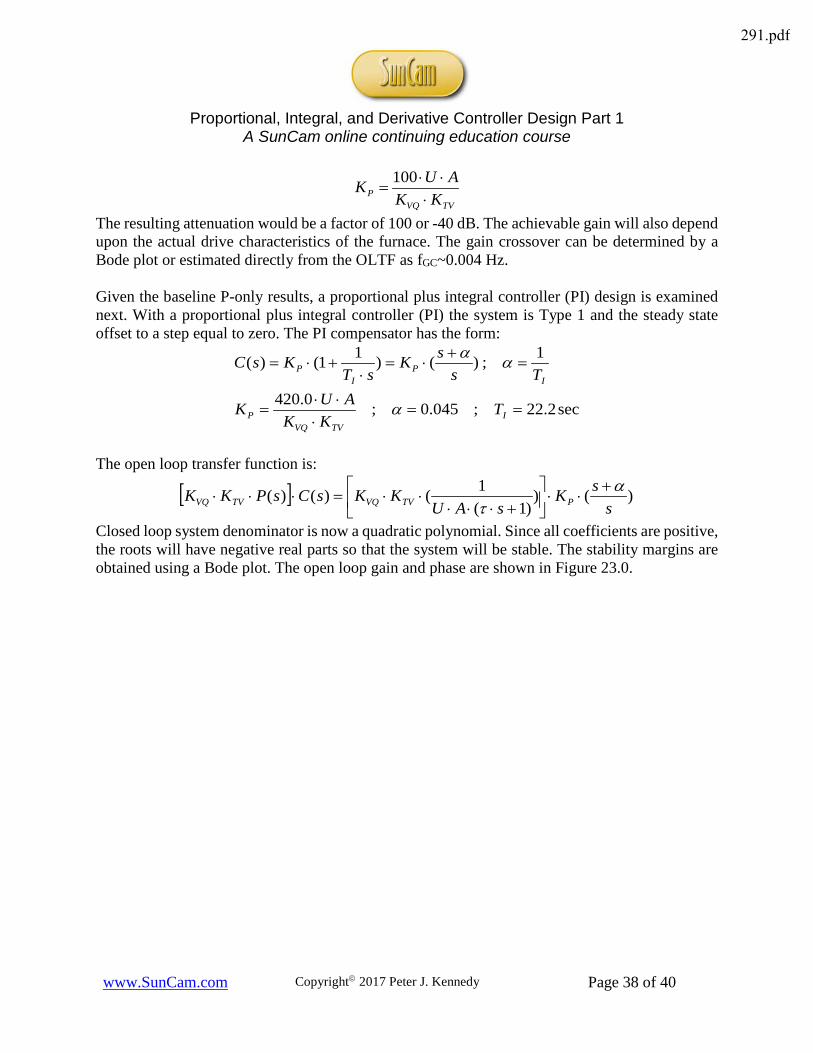
Proportional, Integral, and Derivative Controller Design Part 1
A SunCam online continuing education course
www.SunCam.com Copyright 2017 Peter J. Kennedy Page 38 of 40
TVVQP KK
AUK⋅⋅⋅
=100
The resulting attenuation would be a factor of 100 or -40 dB. The achievable gain will also depend upon the actual drive characteristics of the furnace. The gain crossover can be determined by a Bode plot or estimated directly from the OLTF as fGC~0.004 Hz. Given the baseline P-only results, a proportional plus integral controller (PI) design is examined next. With a proportional plus integral controller (PI) the system is Type 1 and the steady state offset to a step equal to zero. The PI compensator has the form:
sec2.22;045.0;0.420
1;)()11()(
==⋅
⋅⋅=
=+
⋅=⋅
+⋅=
ITVVQ
P
IP
IP
TKK
AUK
TssK
sTKsC
α
αα
The open loop transfer function is:
[ ] )())1(
1()()(s
sKsAU
KKsCsPKK PTVVQTVVQα
τ+
⋅⋅
+⋅⋅⋅
⋅⋅=⋅⋅⋅
Closed loop system denominator is now a quadratic polynomial. Since all coefficients are positive, the roots will have negative real parts so that the system will be stable. The stability margins are obtained using a Bode plot. The open loop gain and phase are shown in Figure 23.0.
291.pdf
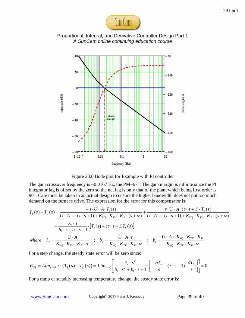
Proportional, Integral, and Derivative Controller Design Part 1
A SunCam online continuing education course
www.SunCam.com Copyright 2017 Peter J. Kennedy Page 39 of 40
phasemargin
Figure 23.0 Bode plot for Example with PI controller The gain crossover frequency is ~0.0167 Hz, the PM~67°. The gain margin is infinite since the PI integrator lag is offset by the zero so the net lag is only that of the plant which being first order is 90°. Care must be taken in an actual design to ensure the higher bandwidth does not put too much demand on the furnace drive. The expression for the error for this compensator is:
[ ]
αατ
αλ
τλ
αττ
ατ
⋅⋅⋅⋅⋅+⋅
=⋅⋅⋅
⋅⋅=
⋅⋅⋅⋅
=
+⋅+⋅+⋅+⋅
⋅=
+⋅⋅⋅++⋅⋅⋅⋅⋅+⋅⋅⋅⋅
++⋅⋅⋅++⋅⋅⋅⋅
⋅⋅⋅−=−
PTVVQ
PTVVQ
PTVVQPTVVQr
Ser
PTVVQ
S
PTVVQ
eCS
KKKKKKAU
bKKK
AUbKKK
AUwhere
sTssTsbsb
ssKKKssAU
sTsAUssKKKssAU
sTAUssTsT
12
12
;;
)()1()(1
)()1()()1(
)()1()()()(
For a step change, the steady state error will be zero since:
0)1(1
))()((1
22
2
00 =
⋅+⋅+−⋅
+⋅+⋅⋅
=−⋅= →→ sTs
sT
sbsbsLimsTsTsLimE Ser
sCSsSSδτδλ
For a ramp or steadily increasing temperature change, the steady state error is:
291.pdf
Proportional, Integral, and Derivative Controller Design Part 1
A SunCam online continuing education course
www.SunCam.com Copyright 2017 Peter J. Kennedy Page 40 of 40
)(
)1(1
))()(( 221
22
2
00
SerSS
SersCSsSS
TTE
sTs
sT
sbsbsLimsTsTsLimE
δδλ
δτδλ
+−⋅=
⋅+⋅+−⋅
+⋅+⋅⋅
=−⋅= →→
The set point will normally not change as a ramp, however the temperature of the environment can so that most likely the steady state error for this case would be:
rampTE erSSδλ ⋅=
Using the definition of KP for this case, λr=0.05 or -25 dB with the PI controller. 9.0 Summary: This completes the course material. The topics covered began with a description of the basic feedback control loop block diagram in section 2 and how the PID relates to the control loop. The relationships between time and frequency domain representations of the block diagram elements were discussed in section 3 followed by the key feedback relationships derived from the block diagram algebra in section 4. The PID control algorithm was described in section 5 which included the frequency domain characterization of the PID (5.1), the effect of each PID term has on response (5.2) and finally different forms of the PID used in actual applications. In section 6 a discussion of specifying control loop performance was presented. PID control loop design methods were provided in section 7. The basic theory was applied to an example; a home heating system, in section 8. Part 2 of this course will discuss the computer implementation of the PID algorithm and interfacing with more advanced control methods. References:
1. Astrom, K., Hagglund T., PID Controllers: Theory, Design, and Tuning, Instrument Society of America, PO Box 12277, Research Triangle Park, NC 27709, ISBN 10: 155617-516-7, ISBN 13: 987-155617-516-9, 1995
2. Astrom, K., Hagglund T., Advanced PID Control, Instrument Society of America, PO Box 12277, Research Triangle Park, NC 27709, ISBN 10-155617-942-1, ISBN-13: 978-1556179-942-6, 2006
3. Kennedy, P, Kennedy, R. , Stabilizing the Line of Sight, LuLu Publishing Company, ISBN-13: 978-0692273562, 2014, http://www.lineofsightstabilization.com
4. Astrom, K., Control System Design Lecture Notes ME 155A UCSB, Chapter 6, https://www.cds.caltech.edu/~murray/courses/cds101/fa02/caltech/astrom.html
291.pdf