Munich Personal RePEc Archive

Profit rates in the developed capitalist

economies: a time series investigation.

Trofimov, Ivan D.

Kolej Yayasan Saad (KYS) – KYS Business School, Malaysia

5 June 2017

Online at https://mpra.ub.uni-muenchen.de/79529/

MPRA Paper No. 79529, posted 05 Jun 2017 13:23 UTC

1

Profit rates in the developed capitalist economies: a time series investigation

Abstract

This paper examines whether there is empirical evidence to support the hypothesis of secular

decline in the economy-wide profit rates as predicted by classical economic theories. We specifically

consider profit rates in the OECD economies based on the national accounts data contained in the

Extended Penn World Table database. In our analysis we use linear trend, Augmented Dickey-Fuller

(ADF) tests, and also allow for structural breaks and instabilities in the series. Results suggest that

profit rates in OECD economies exhibited a wide variety of patterns, including stochastic and

deterministic trends, random walk, reversals, as well as stability. Secular decline (fluctuation around

falling deterministic trend) hypothesis is supported for Canada, Portugal and the USA, while secular

rise is witnessed for Greece and Norway.

Keywords: Profit rate, autoregressive model, structural breaks, trend

JEL Classification: B5, C22, P17

1. Introduction

Theoretical research on the dynamics of profit rates in capitalist economies has been particularly

prolific in the classical and heterodox economic theory with their focus on the inherent instability

and cyclical nature of capitalism. Various other economists (Keynes, Schumpeter) have also

examined profit rates problem, but in a broader context, looking at the overall ability of capitalism to

sustain profit rates opportunities and respectively to expand. Neoclassical economics was also

concerned with the level of profit rates, focusing more narrowly on the health of the corporate

sector and considering profit rates as fundamentals of financial markets performance.

In a related vein, empirical research attempted to establish regularities (tendencies, cycles etc.) in

the actual profit rates’ series and thereby provide factual basis for theories.

The recent revived interest in the subject has been due to declining growth rates in the developed

economies, increased volatility and turbulence in the global economy and structural torsions.

Availability of economic data on profit rates (at national and sectoral level) has also been stimulating

applied research of the topic.

This paper revisits the hypothesis of the secular decline in profit rates (tendency of profit rates to

decline in the long-run) that has been recurrent in classical economics and attempts to validate

empirically whether profit rates in the developed economies have been declining in recent decades.

Inter alia it addresses a number of issues that were not adequately dealt with in previous studies.

Firstly, the analysis of profit rates has to rely on a theoretically sound indicator and acknowledge the

differences that exist between the definition of the profit rate in classical economics and

contemporary definitions of the profit rate which form the base for profit rates indicators in the

modern national accounts. Likewise we have to define the scope of profit rate indicator (economy-

wide rate versus rate in manufacturing sector or in particular industry), as well as variables from

which profit rate indicator is derived (in particular definition of capital stock). Secondly, the majority

of the studies examined profit rates in a single economy (usually as variable in the study of country’s capital accumulation, macroeconomic analysis or the study of country’s structural problems) or in a

small set of economies. This shortcoming stemmed from the lack of available economic data that

could allow comparative analysis. Thirdly, the empirical treatment of profit rates data relied mostly

on visual inspection of profit rate series or on simple regression techniques (e.g. estimation of the

2

linear trend) without proper consideration of unit root properties of the series, the possibility of

trend reversals and breaks in the data. This paper attempts to address these issues by adopting

profit rates’ indicator based on the national accounts, by comparing a large set of the economies,

and by using advanced econometric techniques.

2. Literature review

The early consideration of profit rates dates back to A. Smith and D. Ricardo: the former postulated

the decrease in the level of profit due to competition, while the latter argued that competition

would reduce the profit differences on investments rather than general rate of profit. The latter

would only fall in wages rise, e.g. due to diminishing returns in agriculture and rise in food prices in

agriculture-based economy (Tsoulfidis and Paitaridis, 2012; Ricardo, 1951, p. 120; Mizuta, 2015).

Later, the possibility of insufficient profit generation in capitalism was an area of concern for J. M.

Keynes and J. A. Schumpeter, the former attributing it to financial sector failures, the latter to

possible degeneration of entrepreneurial function in corporate capitalist system (Keynes,

1936/1991, Ch. 24; Argitis, 2003, p. 13; Schumpeter, 1942/1976, Part II).

Profit generation problems come hand in hand with other factors that condition crises and

instabilities in capitalist economies (Edvinsson, 2010, p. 43). Sweezy (1942) and Ramirez (2007) for

instance point to under-consumption and deficient aggregate demand as explanation of crises,

instability and stagnation, as well as to production disproportionality and anarchic nature of

capitalism. Likewise Minsky (1986), Onaran et al. (2012) and Stockhammer (2012) see the origins of

instabilities and crises in debt-led instead of investment-led growth in capitalism.

Overall the complex interplay between finance and financial profits, effective demand, structural

torsions between braches of the economy, debt, and non-financial profits have long been a matter

of investigation in heterodox economics - classical, Keynesian, Schumpeterian and Minskian (Argitis,

2003).

In Marxist literature, the secular decline hypothesis was explained as follows. Capitalist competition

allows innovating capitalists to reap super-normal profits that subsequently dwindle when

innovations swarm through the economy. The need to maintain profits forces capitalists to

introduce labour saving technologies and to ensure sufficient pool of reserve labour (and thereby

low real wages). Together with ongoing capital accumulation, this creates the disparity between

growth in capital accumulation and growth in surplus value (the latter growing slower), leading to

falling rate of profit (Marx, 1867/1967, p. 612). Rate of profit in this formulation is determined by

wages and profits in numerator of the ratio, and capital stock in denominator. Thus, profit rate falls

due to wage and profit factors - declining rate of exploitation, rising real wages and fall in profit

share (Tutan, Campbell, 2005); as well as factors on capital stock side - change in the value

composition of capital and falling capital productivity (Duménil, Lévy, 2001; Wolff, 2003; Mohun,

2009).

It should be noted that while it has been common in heterodox economics to talk about secular

decline and “law of the tendency of the rate of profit to fall”, the precise form of decline

(deterministic decline, cyclical fluctuation around falling trend, or no falling trend at all) has been

debatable. For instance, the works of Marx suggest that this tendency is not inevitable and that

various countervailing factors (and restorative crises of various sorts) may slow down, reverse, or

halt the decline in the rate of profit, meaning thereby in-built resilience in capitalist economies

(Marx, 1867/1967, Vol. III, Ch. 14). Possible countervailing factors could include stagnant real wages

and availability of cheap labour-power (Zachariah, 2009), export of capital and foreign investment

(Brewer, 1990), foreign trade to expand markets (Grossman, 1992, pp. 142-201), diversion of

3

productive investment into financial sector (Guillén, 2007, p. 458). In a related vein, as put by Reuten

(2004, p. 170), certain economists, including N. Kaldor (1957, pp. 597-8, 613), did not consider

secular deterioration hypothesis plausible at all, hypothesizing instead stationarity of profit rates

(Kaldor for instance attributed constant profit rates to constant savings propensities and hence wage

and profit shares, and similar growth rates between output and capital per capita, and hence

constant capital-output ratio). This is one of the well-known Kaldor’s “balanced growth” facts.

On empirical front, the studies of profit rates looked at two distinct issues. Firstly, equalization

tendencies in the rate of profit both across (Glyn, 2007), and within economies (Kambahampati,

1995; Tescari, Vaona, 2014) and convergence to steady-state (Pyo, Nam, 1999) have been

considered, either through time-series analysis, or by probabilistic analysis of the distribution,

equalisation and divergence of the rates of profits (Farjoun, Machover, 1983; Cottrell, Cockshott,

2006).

Secondly, a number of studies looked at trends and cycles in the rates of profit (economy-wide rates,

rates for manufacturing and corporate sector), both in individual developed and developing

economies. The studies included, among others, Weisskopf (1979) and Mohun (2006) for USA;

Mohun (2002) for Australia; Reati (1986) and Poletayev (1992) for Germany; Hayashi and Prescott

(2001) for Japan; Román (1997) for Spain; Erixon (1987) for Sweden. Comparative studies included

Sylvain (2001), Li et al (2007), Daly and Broatbent (2009). Results of the empirical analysis are rather

conflicting: while some studies attest to long-run fall in profit rates (Hayashi, Prescott, 2001), others

provide evidence of periods when profit rates recover and rise (Mohun, 2006), stabilise (Izquierdo,

2007), or experience cycles (Basu, Manolakos, 2010). This can partially be attributed (in addition to

issues of measurement and profit rates’ indicators) to the fact that most empirical studies with the

exception of Basu and Manolakos (2010) tended to rely on visual inspection of the data or the use of

early generation econometric methods (simple linear trends).

This paper does not engage in a theoretical debate on the causes and effects of the fall in the rate of

profit. Instead it attempts to describe statistically and econometrically profit rate patterns and

dynamics. To this purpose it looks which of the theoretical lines in literature (long-run tendency to

decline, versus more diverse behaviour of profit rates) looks more plausible and documents which

events could have contributed to this. Specifically, we attempt to differentiate in profit rates’ series between deterministic trend, deterministic trend with breaks, stochastic trend around non-zero

mean, pure random walk or reversion to historical mean.

3. Methodology

This paper considers the profit rate in the whole economy, instead of examining profit rate in

manufacturing (which was believed to be the core of national economy), given profound changes in

economic structure (specifically the decline in manufacturing and the rise of tertiary sector) that has

been taking place in developed economies over the last few decades.

The paper uses data that includes government sector in both output and capital stock and therefore

do not exclusively look at corporate sector, and also do not provide separate estimates for profit-

type incomes and incomes from self-employment. With regard to residential sector, the data

contained dwellings as part of capital stock. An argument can be raised against this, as residential

sector represents substantial part of total capital stock, while generating much smaller part of total

value added produced (Tutan, Campbell, 2005, p. 15). On the other hand, Edvinsson (2005) argues

that inclusion of residential capital in the total capital stock may be warranted, as “renting out residential buildings is an important source of profit in contemporary society, and the rents paid are

important components of the expenses of wage workers” (p. 192).

4

The empirical analysis makes use of profit rates data contained in Extended Penn World Table

Version 4.0 (EPWT), constructed by D. Foley and A. Marquetti (2012). EPWT itself is based to large

extend on Penn World Table 7.0/PWT 7.0 (Heston, Summers, Aten, 2011). The critical feature of the

EPWT is availability of capital stock series for a large sample of developed economies over 40-50

year period, allowing time series econometric analysis.

The rate of profit variable was constructed as:

( )Y Nw D

K (1)

,where Y is the chain index of real GDP in 2005 purchasing power parity (PPP), K is net fixed

standardised capital stock in 2005 PPP, D is estimated depreciation from K, w is average real wage in

2005 PPP, while N is the number of employed workers.

Variable Y was constructed as product of population and real GDP per capita in 2005 PPP in PWT 7.0.

Variable N was obtained by dividing variable Y by the real GDP per worker in PWT 7.0. Variable K was

computed using perpetual inventory method (PIM) from investment series based on the real

investment share of GDP presented in the PWT 7.0. Variable D was calculated from capital stock

values as:

1t t t tD K I K (2)

Marquetti (2012) acknowledges shortcomings of variables’ construction in PWT. They include

common and high rates of depreciation across economies in the database (the problem that is

inevitable when the task is to ensure comparability of capital stock estimates); inclusion of gross

residential capital formation and change in inventories; short reporting period for investment

variable, as well as ad hoc assumptions about asset life across gross capital formation categories.

Based on EPWT, profit rates’ series were constructed for the following economies (periods) –

Australia, Austria, Belgium, Canada, Ireland, Italy, Luxembourg, Netherlands, New Zealand, Spain,

UK, USA (1964-2008); Denmark, Finland, France, Sweden (1964-2009); Japan, Norway, Switzerland

(1964-2007); Greece (1965-2008); Portugal (1965-2009).

Several data observations were missing for the Netherlands (1965-8) and Norway (1964-7). Newton

interpolation polynomial was used to obtain continuous series for these economies. Germany, being

third largest developed economy was not included in the sample: EPWT contained real wage data

only for West Germany starting from 1982, making sample too short and not including variables

pertaining to former East Germany.

As a first step, we estimated a linear trend model based on the following semi-logarithmic equation:

lnt

t (3)

,where ln is the natural logarithm of the profit rate series, t is the year of observation, and t is

the random disturbance term. Coefficient stands for trend coefficient, i.e. the average annual rate

of change in the profit rate over the respective period. To correct possible autocorrelation, AR terms

were included in the equation.

5

As mentioned by Nelson and Kang (1984), the OLS estimators in the simple trend model tend to be

inconsistent if variable in question is nonstationary. In this case the estimates of the trend are biased

and spurious trends are present. In addition the frequent problems that are encountered in

estimation of the linear trend are the rejection of normality and the presence of heteroscedasticity.

This notwithstanding, following Canjels and Watson (1997), the use of linear trend model may deem

appropriate and correct inference may be obtained, provided efficient estimators, such as Prais-

Winsten are used.

This paper therefore uses conventional linear trend model with AR terms and estimators obtained

using Prais-Winsten procedure. It also considers autoregressive model of Augmented Dickey-Fuller

(ADF) type that addresses above-mentioned problems and encompasses both trend- and difference-

stationarity, i.e.

lnt

t and (4)

lnt

. (5)

Thereby, no prior testing of the series for presence of unit root is required. The autoregressive

model with a time trend has the following form:

1ln ln

t tt , (6)

,where t is time variable andt is random disturbance term. The model has been applied in a

number of contexts to examine univariate dynamics of the series (Athukorala, 2000; Erten, 2011

among others).

Equation (6) may be re-parametrized in a differences form to read:

1(ln ) ln

t tt , (7)

,where 1 .

To correct for possible presence of autocorrelation additional lag of dependent variable (in first

difference) is added. If autocorrelation is not eliminated with 1 lag, additional lags are introduced

until problem is solved. The testing equation is therefore:

1 1(ln ) ln (ln ) (ln )

t t t m tt (8)

The estimation results of this autoregressive equation can be interpreted in the following fashion.

If 0, <0 , the non-zero deterministic trend is present and series revert to this trend after short-

run disturbance.

If ,0 0 , there is no deterministic trend, but series revert to historical mean.

If ,0 0 , series exhibit random walk with zero mean (i.e. past behaviour of profit rate series

gives no indication of the future dynamics, meaning that in the future profit rate may be higher,

smaller or equal to the current value).

6

If ,0 0 , there is random walk with drift (i.e. stochastic trend). In this case, if 0 , it is likely

that future level of profit rate will be greater than current, while if 0 , it is likely that profit rates

will decline in the future.

In the former two cases, an ideal error-correction model is obtained, with statistically significant and

negative γ coefficient, belonging to 1 0 (Engle, Granger, 1987).

In this regard, only first two cases can be considered as a reliable guide to future dynamics of profit

rates. Also, the hypothesis of secular decline in profit rates will be supported when ,0 0 and

,0 0 . The possibility of secular increase is also acknowledged (in this case 0 ).

The long run trend rate from autoregressive estimation above is defined as:

1

b

(9)

If 1 , then equation (3) defined above is obtained.

Regarding interpretation of regression results, it was ensured that coefficient on a lagged

depended variable is statistically significant and that 1 0 holds. Following Pesaran et al

(2001), the t-statistics of coefficient was compared to usual t-value critical bounds, as well as to

Dickey and Fuller (1979) unit root t-statistics (in cases when dependent variable is not stationary in

levels and distribution of t-statistics is non-standard). It was also ensured that coefficients on

respective dummy variables were significant too. First order lagged dependent variable 1

(ln )t

was included to correct autocorrelation, irrespective of term’s significance. Additional lagged terms

(ln )t m were included if autocorrelation persisted (Said, Dickey, 1984). Post-estimation of the

model, usual diagnostic tests for autocorrelation, normality, heteroscedasticity, and ARCH effect

were performed.

Autoregressive ADF-type model was first estimated without dummy variables provided that all

diagnostic tests had been passed. If non-normality of residuals or heteroscedasticity were present,

the dummy variables were introduced and the model was re-estimated. Dummy variables were

based on the year when break or instability in series were likely to occur. Three types of information

to determine dummy variables were obtained: residuals from the ADF model, recursive residuals

and N-step forecasts (Brown et al, 1975). In addition, Quandt-Andrews test (Andrews, 1993) was

performed. As a robustness check, the identified breaks and instabilities were compared to breaks

identified by Bai-Perron (2003) procedure. Regarding type of the dummy variable (impulse or shift),

the above information about the dummy variables was compared to the series’ graphical data.

In case of inconsistency of results between linear trend model and ADF model (with or without

dummy), or between results of these models and the graphical data, additional and more powerful

unit root tests were performed to differentiate between trend stationarity with breaks and unit root

behaviour, as well as between trend stationarity with breaks and unit root with breaks behaviour.

The former type are Zivot-Andrews/ZA (1992) test and Lumsdaine-Papell/LP (1997) test; the latter

type are Lee-Strazicich/LS tests (2003, 2004). ZA and LP tests (with one and two breaks respectively)

were performed in three variants: allowing for shift in the level of series, growth rate of series, or

both. LS tests (with one or two breaks) were performed based on “break” model allowing for structural breaks in both the intercept and the slope under the alternative hypothesis.

7

The linear trend model was then re-estimated, including the dummy variables corresponding to the

breaks identified by ZA, LP and LS tests. It was acknowledged that these tests are not tests for break

timing per se, that dummy variables were thereby likely to be insignificant and that normality and

heteroscedasticity problems were likely to re-appear.

The overall conclusion was made when concordance between the results of the three types of

models (linear trend with dummies based on residuals, autoregressive model with and without

dummies, and linear trend with dummies from ZA, LP and LS tests) was ensured.

4. Empirical results

Before formally testing secular decline hypothesis, the profit rate patterns are presented (Figure 1).

The visual observation suggests that over the study period (1964 to late 2000s) the profit rates were

likely to exhibit downward trends in Austria, Canada, Japan, Portugal, Spain, Switzerland and USA.

Upward trends were likely in Luxembourg and Norway. In other economies either no distinct trend

was present, or trend reversals and random walk behaviour were likely.

[FIGURE 1]

The visual inspection also suggests two distinct patterns for profit rates in most economies – decline

until mid or late 1970s, followed by partial or complete reversal. Early decline was likely present in

all economies, except Luxembourg and perhaps Norway. Complete recovery was witnessed in

Australia, Greece, Italy, Ireland, New Zealand, Netherlands, Sweden and the UK, while partial

recovery or stabilisation was likely in Austria, Belgium, France and Spain. Such countries as

Luxembourg, Norway witnessed not only complete recovery, but also reversal of the trend.

These visual observations however should be interpreted with caution, as spurious regressions and

in particular spurious trends and cyclicality are possible (Granger, Newbold, 1974; Nelson, Kang,

1981).

As to explanation of the phenomenon, Kliman (2012) argues that initial downward trend was

inevitable, due to initially very high profit rates in the early post-WWII period: this was a result of

precedent decline in the value of physical capital and financial assets during turbulent 1930-40s.

Hence, decline in 1960-70s was predetermined, and the low profit rates in 1970s were not seen as

unprecedented, but more as historically normal. Explaining recovery since 1980s, such authors as

Duménil, Levy (2004) and Glyn (2006) point to the profound pro-business political and economic

restructuring that have been occurring, as well as to rising rentier class and “unproductive” sectors,

such as finance and military-industrial complex.

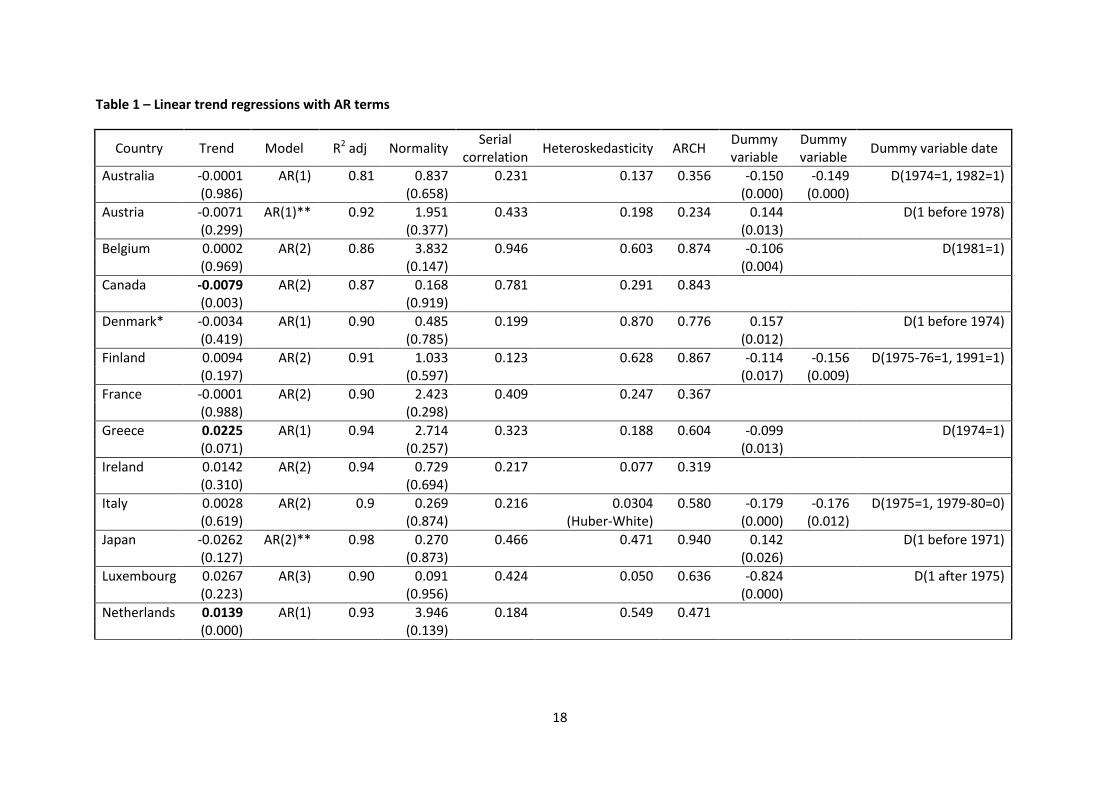
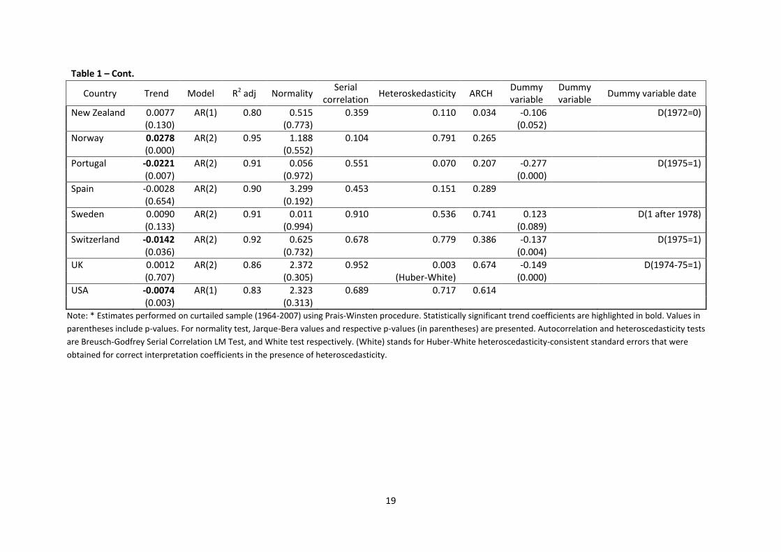
Table 1 presents the results of a linear trend model estimated on the logarithm of the profit rates’ series. Modelling used ARMA conditional least squares (CLS) method based on Gauss-

Newton/Marquardt algorithm, with up to three AR terms included to correct for serial correlation. In

the case of Austria and Japan, CLS method delivered the results that seemed to contradict the data

(specifically, CLS resulted in the positive sign of the trend) and hence ARMA generalized least

squares (GLS) was additionally performed. To ensure normality of the data, shift or impulse dummy

variables were incorporated into trend regression. The choice of dummies was dictated by the

presence of large positive/negative residuals in the trend regression with no dummies, as well as by

visual observation of the series. In the case of Denmark, several specifications of the trend

regression with or without dummies resulted in heteroscedasticity problem; to address it, the

sample was curtailed to 1964-2007. Likewise, heteroscedasticity (at 5% significance level) was

8

present in the case of Italy and the UK even after inclusion of dummy variables; the problem was

addressed by obtaining Huber-White heteroscedasticity-robust standard errors.

[TABLE 1]

Positive trend was observed in 11 cases (Belgium, Finland, Greece, Ireland, Italy, Luxembourg,

Netherlands, New Zealand, Norway, Sweden and the UK). Statistically significant positive trend

coefficients were however present for Greece (at 10% significance level), and Netherlands and

Norway (at 5% level). Negative trend was observed in 10 cases (Australia, Austria, Canada, Denmark,

France, Japan, Portugal, Spain, Switzerland, and the USA). Statistically significant negative trend

coefficient was present for Canada, Portugal, Switzerland and the USA (at 5% significance level).

With regard to Austria and Japan, trend coefficients were insignificant irrespective of the estimation

method. The estimates suggest that profit rates rose by 2.3%, 1.4% and 2.8% per annum over study

period in Greece, Netherlands and Norway respectively. Profit rates declined by 0.8%, 2.2%, 1.4%

and 0.7% per annum over study period in Canada, Portugal, Switzerland and the USA.

Table 2 contains the suggested dates of structural breaks in the series obtained from the four

alternative tests. Negative or positive sign in parentheses represented fall (rise) in series. We note

that Bai-Perron procedure that is more systematic and robust than the four other tests confirms the

timing of breaks and instabilities in the series. Bai-Perron method of sequential testing of I+1 versus I

breaks pointed to the same breaks as Quandt-Andrews test, and also suggested additional break in

1990 for Netherlands, in 1999 for Austria and in 1974 for Portugal. Compared to residuals, recursive

residuals and N-step forecasts, Bai-Perron procedure pointed to at least one similar break in all

economies, except Austria, Canada, Denmark, France, Norway and Portugal. In these latter

economies however the location of the break was quite close to the actual one.

[TABLE 2]

The four tests combined indicate up to three possible instabilities for most of the economies. These

instabilities are clustered in three periods – mid-1970s, early 1980s and late 2000s, with most of the

residuals in these periods being negative. The negative residuals in mid-1970s can be attributed to

the first oil shock, the collapse of the Bretton-Woods system, stagflation and world-wide recession.

Negative residuals in 2009-10 reflect Global Financial Crisis, while instabilities in early 1980s reflect

recession of early 1980s, the rejection of Keynesian economic policies, and certain financial crises

(Latin American debt crisis, and savings and loans crisis in the US). The number of breaks associated

with the Great Recession of the late 2000s was much smaller. Importantly, the breaks occurring in

the 1970s were in most cases due to the fall in the profit rates; in general adverse economic events

and developments resulted in negative residuals and fall in series.

In addition, country-specific factors were prominent. In Australia, the 1982-3 dummy variable

corresponds to the start of economic deregulation, trade liberalisation and movement towards

flexible exchange rate system undertaken by Fraser and Hawke governments. In Belgium, the 1991

dummy variable corresponds to the economic recession of the early 1990s (the worst since the end

of WWII), as well as other structural problems (slow productivity growth, structural unemployment

and other symptoms of Eurosclerosis). In Finland, 1990 dummy reflects the breakup of COMECON

and Soviet Union, and the demise of the foreign trade of Finland with its Eastern European partners.

The dummy variables for the USA (1980, 1982 and 1983-4) relate to the start of the Reagan

presidency and the onset of Reaganomics economic policies, as well as to the deep recession of early

1980s. In Norway, the 2000 dummy variable reflect the period of low oil prices that affected

Norwegian petroleum sector. The impulse dummies in Greece (1974, 1988, 1991), Spain (1975,

1984) and Portugal (1975) can be attributed to political transition to democracy that took place in

9

mid-1970s (demise of regimes of Franco, Salazar and “regime of the colonels”), as well as accession

to European Community (the case of Spain in mid-1980s) and its broad implications. In Italy 1979

dummy reflects deep political crisis during 1979 general elections.

The dummy variables to be used in autoregressive ADF model are presented in Table 3, with dummy

variables respectively set at 1 or 0 to correct structural changes. We note that if structural shifts

were modelled, the dummy variables were set greater or smaller than one after specific date.

[TABLE 3]

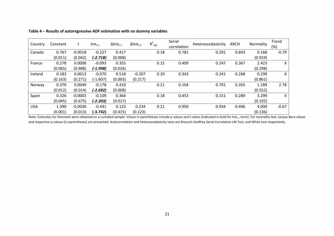
Tables 4 and 5 present the estimates from autoregressive ADF model, the former table - with no

structural breaks, while the latter – with breaks (in impulse or structural shift form). In all cases, it

was ensured that coefficient of the lagged variable lnπt-1 has negative sign. To address possible serial

correlation, additional lag terms of ∆lnπt-1 were included (irrespective of its significance). It was also

ensured that included dummy variables are statistically significant.

[TABLE 4]

In autoregressive ADF model without dummy variables (Table 4), the trend was statistically

significant in the case of Canada, Norway and the USA, with profit rate series falling by 0.79% and

0.67% per annum respectively in Canada and the USA during 1964-2008 period. In Norway, profit

rates were rising by 2.78% per annum over 1964-2007 period. For other countries in question, trend

rate was not estimated due to insignificance of trend coefficient. Using Dickey-Fuller critical values,

the coefficient of lnπt-1 term was likewise significant only for the USA, while using conventional t-

statistics critical values it was also significant for Canada and Norway.

It was therefore concluded that in these economies profit rates followed non-zero deterministic

trend model with series reverting to trend after short disturbance (β ≠ 0, γ < 0). With regard to other economies, coefficient of lnπt-1 was significant at 5% t-statistics critical value in France and Spain,

suggesting that series in these economies reverted to historical mean (β = 0, γ < 0). In Ireland, series followed random walk with zero mean (β = 0, γ = 0).

The ADF model results fall in line with estimates of linear trend in Table 1, both in terms of

significance and sign of trend. Both models suggest that profit rates in Canada and the USA

deteriorated around negative deterministic trend and in Norway around positive deterministic

trend. In the case of France, Ireland and Spain, ADF model confirmed the results of the linear trend

model that pointed to the absence of deterministic trend and suggested either mean reversion or

random walk as alternatives.

[TABLE 5]

ADF model with dummy variables (Table 5) showed that trend was statistically significant in

Denmark, Greece, Portugal, Switzerland and the UK, with profit rates deteriorating by 2.33%, 2.92%,

0.83% and 1.46% per annum in Denmark, Portugal, Switzerland and the UK over the examined

periods. In Greece, profit rates were increasing by 2.13% per annum over 1965-2008 period. The

coefficient of lnπt-1 term was significant in Finland, New Zealand and Switzerland (using Dickey-Fuller

critical values), and in Austria, Belgium, Greece, Japan, Luxembourg and Portugal (using t-statistics

5% critical value). It is thus concluded that profit rates in Greece, Portugal and Switzerland followed

non-zero deterministic trend with likely reversion to trend after disturbance (β ≠ 0, γ < 0). Deterministic trend was positive in Greece and negative in other two economies. Series in Austria,

Belgium, Finland, Japan, Luxembourg and New Zealand were likely to revert to historical mean (β =

10

0, γ < 0). Profit rates in Australia, Italy, Netherlands and Sweden were following random walk with

zero mean (β = 0, γ = 0), while series in Denmark and the UK were likely to follow stochastic trend (random walk with drift), as β ≠ 0 but γ = 0. In both Denmark and the UK, β < 0 suggesting that profit rates were likely to decline in the future relative to the current level.

The comparison of autoregressive ADF model with linear trend model (Table 1) demonstrates

similarity of results for most of the economies: Australia and Sweden (negative, but insignificant

trend with series exhibiting random walk); Austria and Japan (negative but insignificant trend with

series reverting to historical mean); Belgium, Finland, Italy, Luxembourg and New Zealand (positive,

but insignificant trend with series reverting to historical mean or, in the case of Italy, following

random walk with zero mean); Denmark and the UK (positive or negative insignificant trend with

series following stochastic trend); Greece (positive and significant trend in both models); and

Portugal and Switzerland (negative and significant trend in both models). For the Netherlands,

results are contradictory. While linear trend model suggests statistically significant positive

deterministic trend, autoregressive ADF model pointed to random walk behaviour with zero mean.

The presence of certain results’ inconsistencies as well as the low power of ADF test necessitated the

use of unit root tests with structural breaks. Results are presented in Tables 6 and 7.

The tests were run on the log of profit rate series, allowing for a maximum of 8 lag terms. According

to ZA test (models with trend, intercept, and more general model with both trend and intercept),

trend stationarity hypothesis is accepted only for Canada (model with intercept), while in all other

cases series were likely to contain unit root. According to LP test (with same types of models as in ZA

test), trend stationary is accepted for Italy and Portugal (trend plus intercept), Spain (trend plus

intercept as well as trend models), and the USA (model with intercept).

[TABLE 6]

Based on LS tests (1 or 2 breaks in series), trend stationarity with break was expected for a larger

number of series, excluding France, Italy, Luxembourg, Netherlands, New Zealand, Sweden,

Switzerland and the UK.

[TABLE 7]

In cases when trend stationarity was expected, the linear trend model was re-estimated with breaks

suggested by ZA, LP and LS tests (in either impulse or shift form). It is born in mind that these tests

are not the tests for the presence of structural break, that the inclusion of these break dates does

not necessarily allow for normality (or absence of heteroscedasticity), and that break dates may not

correspond to actual economic events or developments. Results of the modified linear trend model

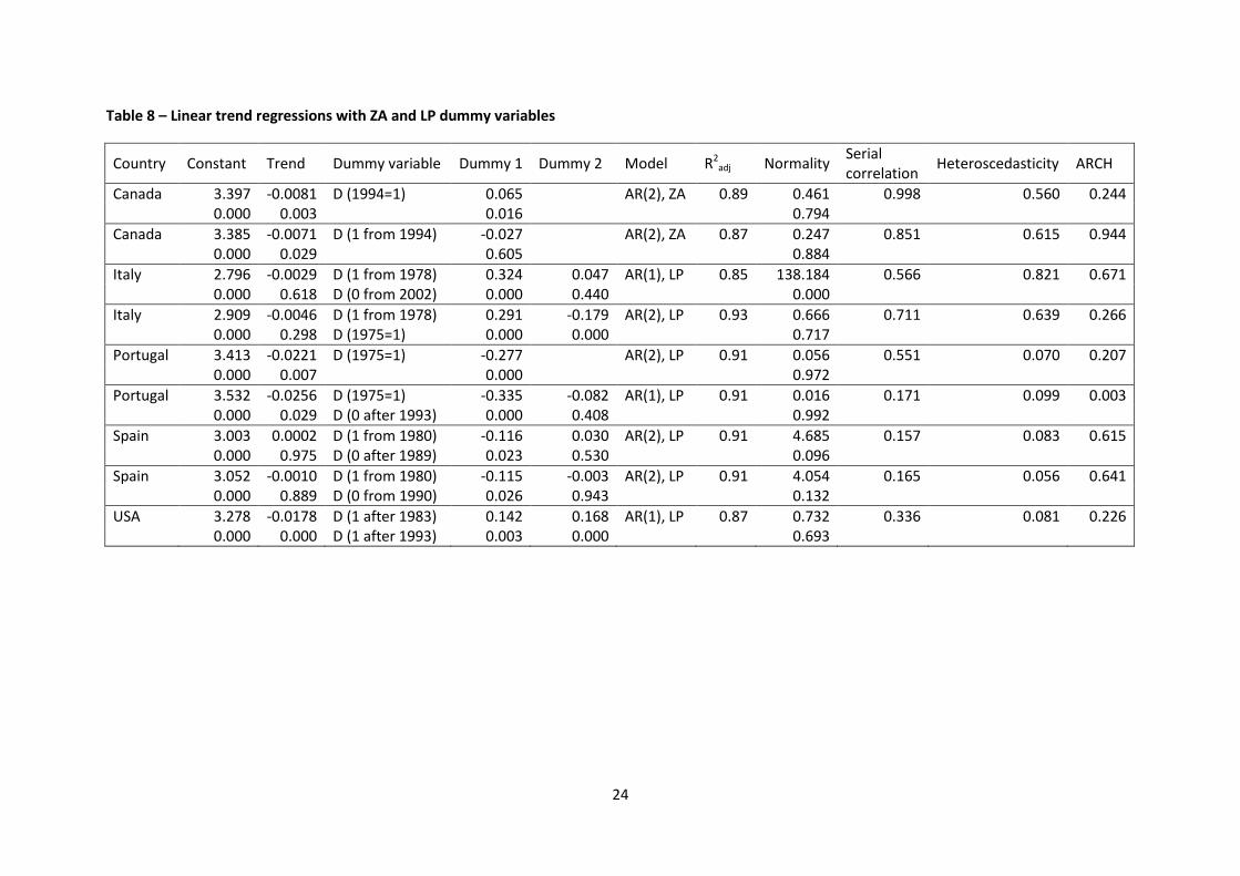
are presented in Tables 8 and 9.

Trend model with breaks from ZA and LP tests (Table 8) demonstrates that coefficient of trend was

not significant in the case of Italy and Spain, thereby confirming earlier result of the absence of

deterministic trend in these countries’ profit rates. In contrast, trend coefficient was significant for

Canada, Portugal and the USA.

[TABLE 8]

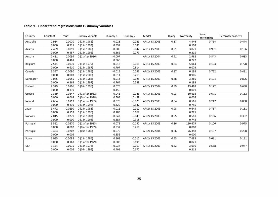
With regard to trend model with breaks from LS tests (Table 9), trend coefficients were significant

for Canada, Portugal and the USA (negative trend), as well as for Greece and Norway (positive

trend). This again is in concordance with the results of ADF and linear trend models.

11

[TABLE 9]

Conclusion

The paper attempted to contribute to empirical debate on the direction of economy-wide profit

rates in the developed economies. It employed comparable national accounts data spanning the

period of 5 decades. It employed a battery of econometric tests and techniques: linear trend model

with autoregressive terms and dummy variables; tests for the presence of structural breaks;

Augmented Dickey-Fuller (ADF) model of a general form with and without dummy variables; Zivot-

Andrews (ZA), Lumsdaine-Papell (LP) and Lee-Strazicich (LS) unit root tests with structural breaks; as

well as linear trend model with dummy variables based on breaks from these tests.

The results demonstrated substantial consistency across tests conducted, as well as consistency

between tests and visual observation of the data. Specifically, conventional linear trend model

suggested negative deterministic trend for Canada, Portugal, Switzerland and the USA, and positive

deterministic trend for Greece, Netherlands and Norway. Two versions of autoregressive ADF model

also demonstrated deterministic trends for these economies with the exception of Netherlands.

Linear trend models based on ZA, LP and LS fully confirmed autoregressive ADF model results (with

Switzerland being the exception). Other economies had non-deterministic changes in their rates of

profit.

Overall, secular decline in profit rates took place in Canada, the USA and Portugal, arguably giving

support to Marx’s hypothesis of the tendency of the profit rate to fall along deterministic trend. For

the US it confirms earlier results by Basu and Manolakos (2010). Some support of the hypothesis

could have been provided for profit rates in Netherlands, but only if linear trend model is considered

in isolation from other tests. Likewise, there is support of secular decline hypothesis for Switzerland,

but only if results of ZA, LP and LS tests are disregarded. Secular rise in profit rates has been

witnessed in Greece and Norway, and this result is in sharp contrast to the classical hypothesis. In

the former case this could be attributed to rapid transformation of the economy in 1960-80s from a

relatively low base; in the latter case increase in economy-wide profit could have been boosted by

the growth of oil sector. In Portugal, profit rates seemed to follow a specific pattern of secular

decline interrupted by crises, with rates after each crisis been lower than before it (i.e. stepwise

decline).

With regard to Denmark and the UK, profit rates in these economies appear to have experienced

random walk with drift, pointing to stochastic trends and long waves, thereby giving some support

to hypothesis of cyclical movements in profit rates. This has to be confirmed formally by isolating

cyclical component in the series. In addition, for Denmark, the stochastic trend result was obtained

on series that were trimmed due to heteroscedasticity; the result contradicts visual inspection of the

data, as well as LS test. Autoregressive model also points to significant and negative trend

coefficient. If full series were considered, it arguably could show negative deterministic trend and

thus confirm secular decline hypothesis.

For the group of economies where profit rates followed random walk with zero mean (Australia,

Ireland, Italy and Sweden), the hypothesis of Kaldor-like stability/stationarity was not tested (this

could have been achieved by performing ADF test with no trend). It is however possible to estimate

innovation variance of the random walk component (Cochrane, 1988, p. 895) and thereby select

those series with the smallest random walk component. Overall, based on tests performed we argue

that profit rates in these economies give no support to either secular decline or decline with cyclical

component hypotheses.

12

Those economies that experienced reversion of profit rates to historical means (Austria, Belgium,

Finland, France, Japan, Luxembourg, New Zealand and Spain) are likely to demonstrate the case of

restorative crises, where previous decline in profit rates was reversed, partially or substantially. This

case neither supports nor contradicts secular decline hypothesis; more definitive conclusions would

require longer series to investigate. Similar observation may be made regarding countervailing

factors that are presumed to operate in medium and long-run (Shaikh, 1992).

Overall, the behavior of profit rates was rather diverse, and thus it is unlikely that “universal profit rates’ laws” hold or only one hypothesis is correct.

The future research of profit rates dynamics may be pursued in the following directions. Firstly, the

future analysis will have to address the wide diversity of profit rate patterns across the economies

(including the economies that are supposed to demonstrate similar profit rate dynamics) as well

similarities of profit rates’ patterns across the economies with different political-economic and social

settings. The paper pointed to some of the facts that require explanation – similar profit rates’ dynamics in the closely integrated economies of Canada and the USA, but rather different dynamics

in closely related economies in Europe (e.g. Belgium and Luxembourg); different profit rates

directions in formerly developing economies of Portugal and Greece; similarities in profit rates’ patterns in Greece and Norway. The type of analysis that would be needed would require looking at

national forms of capitalism and unique constellation of factors in each economy in question.

Alternatively, the analysis of a single factor (economic integration, or one of the countervailing

factors, such as financialization, trade liberalization) on the rates of profit in a range of economies

may be undertaken. These types of investigation would therefore allow unpacking the operation of

countervailing tendencies and explain how restorative crises work through the economic system.

Secondly, while the focus of this paper has been on developed economies, an alternative research

avenue could be the study of profit rates in transition and developing economies (or few remaining

centrally planned economies), with a different set of factors likely to be salient and different

patterns discovered. Also, the dynamics of profit rates would clearly be diverse if sectoral or

industrial profit rates were considered. In this connection it would be instructive to examine profit

rates in the context of structural change or sectoral re-allocation of capital. Finally, future research

may be carried in “microeconomic” fashion, in line with above mentioned works by Farjoun and Machover (1983), i.e. by examining profit rates across firms, narrow industries, and by considering

distributions of profit rates.

13

References

Andrews, D. (1993), “Tests for Parameter Instability and Structural Change with Unknown Change

Point,” Econometrica, 61 (4), 821-856.

Argitis, G. (2003), “Finance, Instability and Economic Crisis: The Marx, Keynes and Minsky Problems

in Contemporary Capitalism,” presented in the Conference ‘Economics for the Future’, Cambridge, September 17-19, 2003.

Athukorala, P.-C. (2000), “Manufactured Exports and Terms of Trade of Developing Countries:

Evidence from Sri Lanka,” Journal of Development Studies, 36 (5), 89-104.

Bai, J., and P. Perron (2003), “Computation and Analysis of Multiple Structural Change Models,” Journal of Applied Econometrics, 18 (1), 1-22.

Basu, D., and P. Manolakos (2010), “Is There a Tendency for the Rate of Profit to Fall? Econometric

Evidence for the US Economy, 1948-2007,” University of Massachusetts – Amherst Economics

Department Working Paper Series, 1-1-2010.

Brewer, A. (1990), Marxist Theories of Imperialism: A Critical Survey, New York: Routledge & Kegan

Paul.

Brown, R. L., Durbin, J., and J. M. Evans (1975), “Techniques for Testing the Constancy of Regression Relationships over Time,” Journal of the Royal Statistical Society, Series B, 35, 149-192.

Canjels, E., and Watson, M. W. (1997), “Estimating Deterministic Trends in the Presence of Serially Correlated Errors,” Review of Economics and Statistics 79 (2), 184-200.

Chow, G. C. (1960), “Tests of Equality between Sets of Coefficients in Two Linear Regressions,” Econometrica 28 (3), 591-605.

Cochrane, J. H (1988), “How Big Is The Random Walk in GNP?” Journal of Political Economy, 96 (5),

893-920.

Cottrell, A. and P. Cockshott (2006), “Demography and the Falling Rate of Profit,” Indian Development Review, 4 (1), 39-59.

Daly, K., and B. Broadbent (2009), “The Savings Glut, the Return on Capital and the Rise in Risk Aversion,” Global Economics Paper No 185, Goldman Sachs Global Economics, Commodities and

Strategy Research.

Dickey, D. A. and W. A. Fuller (1979), “Distribution of the Estimators for Autoregressive Time Series with a Unit Root,” Journal of the American Statistical Association, 74 (366), 427-431.

Duménil, G. and D. Lévy (2004), Capital Resurgent. Roots of the Neoliberal Revolution, Cambridge:

Harvard University Press.

Edvinsson, R. (2005), Growth, Accumulation and Crisis: With New Macroeconomic Data for Sweden 1800-2000, Stockholm: Almqvist & Wiksell International.

14

Engle, R. F. and C. W. J. Granger (1987), “Cointegration and Error Correction: Representation, Estimation and Testing,“ Econometrica, 55 (2), 251-276.

Erixon, L. (1987), Profitability in Swedish Manufacturing: Trends and Explanations, Stockholm:

Almqvist & Wiksell International.

Erten, B. (2011), “North-South terms-of-trade trends from 1960 to 2006,” International Review of Applied Economics, 25 (2), 171-184.

Farjoun, E. and M. Machover (1983), Laws of Chaos: A Probabilistic Approach to Political Economy,

London: Verso.

Foley, D. and A. Marquetti (2012), “Extended Penn World Tables: Economic Growth Data Assembled

from the Penn World Tables and Other Sources,” Available at

https://sites.google.com/a/newschool.edu/duncan-foley-homepage/home/EPWT

Glyn, A. (2006), Capitalism Unleashed – Finance, Globalisation and Welfare, Oxford: Oxford

University Press.

Glyn, A. (2007), “Globalisation and Profitability Since 1950: A Tale of Two Phases?” in ed., A. Shaikh,

Globalization and the Myths of Free Trade: History, Theory, and Empirical Evidence, New York:

Routledge.

Granger, C. and P. Newbold (1974), “Spurious Regressions in Econometrics,” Journal of Econometrics, 2, 111-120.

Grossman, H. (1992), The Law of Accumulation, London: Pluto Press.

Guillén, A. (2014), “Financialization and Financial Profit,” Brazilian Journal of Political Economy, 34

(3), 451-470.

Hayashi, F. and E. C. Prescott (2002), “The 1990s in Japan: A Lost Decade,” Review of Economic Dynamics, 5(1), 206-235.

Heston, A., Summers, R., and B. Aten (2011), “Penn World Table Version 7.0,” Philadelphia: Center

for International Comparisons of Production, Income and Prices. Available at

http://pwt.econ.upenn.edu/.

Kaldor, N. (1957), “A Model of Economic Growth,” Economic Journal, 67 (268), 591-624.

Kambahampati, U. S. (1995), “The Persistence of Profit Differentials in Indian Industries,” Applied Economics, 27 (4), 353-361.

Keynes, J. M. (1936/1991), The General Theory of Employment, Interest and Money, Cambridge:

Cambridge University Press.

Kliman, A. (2012), The Failure of Capitalist Production: Underlying Causes of the Great Recession.

London: Pluto Press.

15

Li, M., Feng, X. and A. Zhu (2007),”Long Waves, Institutional Changes and Historical Trends: A Study

of the Long Term Movement of the Profit Rate in the Capitalist World-Economy,” Journal of World-System Research, 13 (1), 33-54.

Lee, J. and M. Strazicich (2003), “Minimum Lagrange multiplier Unit Root Test with Two Structural Breaks,” The Review of Economics and Statistics, 85 (4), 1082-1089.

Lee, J., and M. Strazicich (2004), “Minimum Lagrange Multiplier Unit Root Test with One Structural

Break,”Appalachian State University, Department of Economics, Unpublished Manuscript.

Lumsdaine, R. and D. H. Papell (1997), “Multiple Trend Breaks and the Unit Root Hypothesis,” Review of Economics and Statistics, 79 (2), 212-218.

Marx, K. (1867/1967), Capital, Volume I, New York: International Publishers.

Minsky, H. (1986), Stabilising an Unstable Economy, New Haven: Yale University Press.

Mizuta, K. (2015), “Ricardo’s Theory of International Trade and Capital Accumulation,” presented at

the 31st

Seminar of Ricardo Society, Chu University, August 1, 2015.

Mohun, S. (2002), “The Australian Rate of Profit, 1965-2001,” Journal of Australian Political Economy, 52, December, 83-112.

Mohun, S. (2006), “Distributive Shares in the US Economy, 1964-2001,” Cambridge Journal of Economics, 30(3), 347-370.

Mohun, S. (2009), “Aggregate Capital Productivity in the US Economy, 1964-2001,” Cambridge Journal of Economics, 33 (5), 1023-1046.

Nelson, C. R. and H. Kang (1984), “Pitfalls in the Use of Time as an Explanatory Variable,” Journal of Business and Economic Statistics, 2 (1), 73-82.

Onaran, O., Stockhammer, E. and L. Grafl (2010), “Financialisation, Income Distribution and

Aggregate Demand in the USA,” Cambridge Journal of Economics, 35 (4), 637-661.

Pesaran, M. H., Shin, Y. and R. J. Smith (2001), “Bounds Testing Approaches to the Analysis of Long

Run Relationships,” Journal of Applied Econometrics, 16 (3), 289-326.

Poletayev, V. A. (1992), ”Long Waves in Profit Rates in Four Countries,” in eds., A. Kleinknecht, E.

Mandel, and I. Wallerstein, New Findings in Long Wave Research, New York: St. Martin Press, pp.

151-168.

Pyo, H. K., and K. Nam (1999), “A Test of the Convergence Hypothesis by Rates of Return to Capital:

Evidence from OECD Countries,” Tokyo: Centre for International Research on the Japanese Economy,

Discussion Paper Series No. 99-CF-51.

Ramirez, M. D. (2007), “Marx, Wages, and Cyclical Crises: A Critical Interpretation,” Contributions to Political Economy, 26 (1), 27-41.

Reati, A. (1986), “The Rate of Profit and the Organic Composition of Capital in West German Industry

from 1960 to 1981,” Review of Radical Political Economics, 18 (1/2), 56-86.

16

Reuten, G. (2004), “Zirkel Vicieux” or Trend Fall? The Course of the Profit Rate in Marx’s Capital III,” History of Political Economy, 36 (1), 163-186.

Ricardo, D. (1951), “On the Principles of Political Economy and Taxation,” in P. Sraffa, The Works and Correspondence of David Ricardo. Volume I, Cambridge: Cambridge University Press.

Román, M. (1997), Growth and Stagnation of the Spanish Economy. The long Wave: 1954–1993,

Aldershot: Avebury.

Said, S. E. and D. A. Dickey (1984), “Testing for Unit Roots in ARMA Models of Unknown Order,” Biometrika, 71 (3), 599-607.

Schumpeter, J. A. (1942/1976), Capitalism, Socialism, and Democracy, New York: Harper and

Brothers.

Shaikh, A. (1992), “The Falling Rate of Profit as the Cause of Long Waves: Theory and Empirical

Evidence,” in ed., A. Kleinknecht, New Findings in Long Wave Research, London: Macmillan.

Stockhammer, E. (2012), “Financialisation, Income Distribution and the Crisis,” Investigación Económica, 71 (279), 39-70.

Sweezy, P. M. (1942), The Theory of Capitalist Development, New York: Monthly Review Press.

Sylvain, A. (2001), “Rentabilité et Profitabilité du Capital: le Cas de Six Pays Industrialisés,”Économie et Statistique, 341-342, 129-152.

Tescari, S. and A. Vaona (2014), “Regulating Rates of Return Do Gravitate in US Manufacturing!” Metroeconomica, 65(3), 377-396.

Tsoulfidis, L. and D. Paitaridis (2012), “Revisiting Adam Smith's Theory of the Falling Rate of Profit,”

International Journal of Social Economics, 39 (5), 304 – 313.

Tutan, M. and A. Campbell (2005), “The Post 1960 Rate of Profit in Germany,” Izmir University of

Economics, Working Papers in Economics, Working Paper No. 05/01.

Weisskopf, T. (1979), “Marxian Crisis Theory and the Rate of Profit in the Postwar US Economy,”

Cambridge Journal of Economics, 3(4), 341-378.

Wolff, E. N. (2003), “What’s Behind the Rise in Profitability in the US in the 1980s and 1990s?”

Cambridge Journal of Economics, 27 (4), 479-499.

Zachariah, D. (2009), “Determinants of the Average Profit Rate and the Trajectory of Capitalist

Economies,” Bulletin of Political Economy, 3 (1), 13-36.

Zivot, E. and D. W. K. Andrews (1992), “Further Evidence on the Great Crash, the Oil-price Shock,

and the Unit-root Hypothesis,” Journal of Business and Economic Statistics, 10 (3), 251-270.

17

Figure 1 - Profit rates in OECD economies

18

Table 1 – Linear trend regressions with AR terms

Country Trend Model R2 adj Normality

Serial

correlation Heteroskedasticity ARCH

Dummy

variable

Dummy

variable Dummy variable date

Australia -0.0001 AR(1) 0.81 0.837 0.231 0.137 0.356 -0.150 -0.149 D(1974=1, 1982=1)

(0.986) (0.658) (0.000) (0.000)

Austria -0.0071 AR(1)** 0.92 1.951 0.433 0.198 0.234 0.144 D(1 before 1978)

(0.299) (0.377) (0.013)

Belgium 0.0002 AR(2) 0.86 3.832 0.946 0.603 0.874 -0.106 D(1981=1)

(0.969) (0.147) (0.004)

Canada -0.0079 AR(2) 0.87 0.168 0.781 0.291 0.843

(0.003) (0.919)

Denmark* -0.0034 AR(1) 0.90 0.485 0.199 0.870 0.776 0.157 D(1 before 1974)

(0.419) (0.785) (0.012)

Finland 0.0094 AR(2) 0.91 1.033 0.123 0.628 0.867 -0.114 -0.156 D(1975-76=1, 1991=1)

(0.197) (0.597) (0.017) (0.009)

France -0.0001 AR(2) 0.90 2.423 0.409 0.247 0.367

(0.988) (0.298)

Greece 0.0225 AR(1) 0.94 2.714 0.323 0.188 0.604 -0.099 D(1974=1)

(0.071) (0.257) (0.013)

Ireland 0.0142 AR(2) 0.94 0.729 0.217 0.077 0.319

(0.310) (0.694)

Italy 0.0028 AR(2) 0.9 0.269 0.216 0.0304 0.580 -0.179 -0.176 D(1975=1, 1979-80=0)

(0.619) (0.874) (Huber-White) (0.000) (0.012)

Japan -0.0262 AR(2)** 0.98 0.270 0.466 0.471 0.940 0.142 D(1 before 1971)

(0.127) (0.873) (0.026)

Luxembourg 0.0267 AR(3) 0.90 0.091 0.424 0.050 0.636 -0.824 D(1 after 1975)

(0.223) (0.956) (0.000)

Netherlands 0.0139 AR(1) 0.93 3.946 0.184 0.549 0.471

(0.000) (0.139)

19

Table 1 – Cont.

Country Trend Model R2 adj Normality

Serial

correlation Heteroskedasticity ARCH

Dummy

variable

Dummy

variable Dummy variable date

New Zealand 0.0077 AR(1) 0.80 0.515 0.359 0.110 0.034 -0.106 D(1972=0)

(0.130) (0.773) (0.052)

Norway 0.0278 AR(2) 0.95 1.188 0.104 0.791 0.265

(0.000) (0.552)

Portugal -0.0221 AR(2) 0.91 0.056 0.551 0.070 0.207 -0.277 D(1975=1)

(0.007) (0.972) (0.000)

Spain -0.0028 AR(2) 0.90 3.299 0.453 0.151 0.289

(0.654) (0.192)

Sweden 0.0090 AR(2) 0.91 0.011 0.910 0.536 0.741 0.123 D(1 after 1978)

(0.133) (0.994) (0.089)

Switzerland -0.0142 AR(2) 0.92 0.625 0.678 0.779 0.386 -0.137 D(1975=1)

(0.036) (0.732) (0.004)

UK 0.0012 AR(2) 0.86 2.372 0.952 0.003 0.674 -0.149 D(1974-75=1)

(0.707) (0.305) (Huber-White) (0.000)

USA -0.0074 AR(1) 0.83 2.323 0.689 0.717 0.614

(0.003) (0.313)

Note: * Estimates performed on curtailed sample (1964-2007) using Prais-Winsten procedure. Statistically significant trend coefficients are highlighted in bold. Values in

parentheses include p-values. For normality test, Jarque-Bera values and respective p-values (in parentheses) are presented. Autocorrelation and heteroscedasticity tests

are Breusch-Godfrey Serial Correlation LM Test, and White test respectively. (White) stands for Huber-White heteroscedasticity-consistent standard errors that were

obtained for correct interpretation coefficients in the presence of heteroscedasticity.

20

Table 2 – Tests of breaks and instabilities in profit rates’ series

Country Recursive residuals N-step forecasts Residuals Quandt-

Andrews

Australia 1974(-) 1978-9(+) 1974(-) 1974(-) 1982(-) 1983(+) 1984

Austria 1971(+) 1975(-) 1978(-) 1974

Belgium 1975(-) 1991(-) 1975(-) 1975(-) 1981(-) 1991(-) 1974

Canada 1982(-) 1994(+) 1982(-) 1983(+) 1994(+) 1976

Denmark* 1977-8(+) 1977-8(+) 1974(-) 1977-8(+) 1994(+) 1971

Finland 1974-5(-) 1997(+) 1975(-) 1997(+) 1975(-) 1990-1(-) 1997

France 1975(-) 1982(+) 2009(-) 1974-5(-) 1983(-) 1973

Greece 1974(-) 1988(+) 1974(-) 1974(-) 1988(+) 1991(+) 1993

Ireland 1974(-) 1987(+) 1974(-) 1987(+) 1974(-) 1980(-) 1994(+) 1995

Italy 1975(-) 1979(+) 1975(-) 1975(-) 1979(+) 1979

Japan 1972(+) 1985(+) 1971(-) 1974(-) 1985(+) 1974

Luxembourg 1975(-) 1977(-) 1975(-) 1969(+) 1975(-) 1977(-) 1984

Netherlands 1976(+) 1994(+) 1974-5(-) 1976(+) 1994(+) 1984

New Zealand 1972(+) 1983(+) 1972(+) 1983(+) 1969(+) 1972(+) 1974(-) 1989

Norway 1975(-) 1979(+) 1975(-) 1979(+) 1986(-) 1993

Portugal 1974-5(-) 1974-5(-) 2000

Spain 1980(+) 1997(-) 1980(+) 1980(+) 1981(-) 1997(-) 1971

Sweden 1973(+) 1976-7(-) 1982(+) 1973(+) 1976-7(-) 1982(+) 1994

Switzerland 1976(+) 1989(+) 1975(-1) 1975(-) 1989(+) 2001(-) 1975

UK 1974(-) 1978-9(+) 1972-5(-) 1976(+) 1983

USA 1971(+) 1980(-) 1994(+) 1980(-) 1982(-) 1994(+) 1970

Note: * Estimates performed on curtailed sample (1964-2007).

Table 3 – Dummy variables in autoregressive ADF model

Country Dummy variables Country Dummy variables

Australia 1974=1 1983=0 Luxembourg 1975=1 1977=1 1981=1

Austria 1975=1 1978=1 Netherlands 1975=1 1994=0

Belgium 1975=1 1991=1 New Zealand 1972=0 1983=0

Canada 1982=1 Norway 1975=1

Denmark* 1974=1 Portugal 1975=1

Finland 1975=1 1990-1=1 1997=1 Spain 1997=1

France 1975=1 Sweden 1976-7=1

Greece 1974=1 1988=0 1991=0 Switzerland 1975=1

Ireland 1974=1 UK 1972-5=1

Italy 1975=1 1979=0 USA 1980=1

Japan No dummies

Note: * Estimates performed on curtailed sample (1964-2007).

21

Table 4 – Results of autoregressive ADF estimation with no dummy variables

Country Constant t lnπt-1 ∆lnπt-1 ∆lnπt-2 R2

adj Serial

correlation Heteroscedasticity ARCH Normality

Trend

(%)

Canada 0.767 -0.0018 -0.227 0.417 0.18 0.781 0.291 0.843 0.168 -0.79

(0.011) (0.042) (-2.718) (0.008) (0.919)

France 0.278 0.0000 -0.093 0.355 0.15 0.409 0.247 0.367 2.423 X

(0.065) (0.988) (-1.998) (0.026) (0.298)

Ireland 0.183 0.0013 -0.070 0.518 -0.207 0.20 0.343 0.241 0.268 0.299 X

(0.163) (0.271) (-1.607) (0.003) (0.217) (0.861)

Norway 0.370 0.0049 -0.178 0.410 0.21 0.104 0.791 0.265 1.189 2.78

(0.012) (0.014) (-2.692) (0.008) (0.552)

Spain 0.326 -0.0003 -0.109 0.364 0.18 0.453 0.151 0.289 3.299 X

(0.045) (0.675) (-2.203) (0.017) (0.192)

USA 1.390 -0.0030 -0.441 0.123 0.234 0.21 0.950 0.934 0.496 4.000 -0.67

(0.001) (0.013) (-3.742) (0.415) (0.123) (0.136) Note: Estimates for Denmark were obtained on a curtailed sample. Values in parentheses include p-values and t-ratios (indicated in bold for lnπt-1 term). For normality test, Jarque-Bera values

and respective p-values (in parentheses) are presented. Autocorrelation and heteroscedasticity tests are Breusch-Godfrey Serial Correlation LM Test, and White test respectively.

22

Table 5 – Results of autoregressive ADF estimation with dummy variables

Country Constant t lnπt-1 ∆lnπt-1 Dummy1 Dummy2 Dummy timing R2

adj Serial

correlation Heteroscedasticity ARCH Normality Trend (%)

Australia 0.319 -0.0005 -0.103 0.079 -0.213 0.170 D (1974=1) 0.36 0.357 0.188 0.857 0.127 X

(0.225) (0.552) (-1.177) (0.557) (0.001) (0.006) D (1983=1)

(0.938)

Austria 0.267 0.0005 -0.098 -0.153 -0.149 -0.149 D (1975=1) 0.41 0.342 0.837 0.696 0.651 X

(0.059) (0.450) (-2.219) (0.246) (0.002) (0.002) D (1978=1)

(0.722)

Belgium 0.253 6.1E-05 -0.093 0.220 -0.160 -0.144 D (1975=1) 0.32 0.908 0.693 0.445 4.007 X

(0.110) (0.931) (-1.696) (0.106) (0.006) (0.013) D (1991=1)

(0.135)

Denmark* 0.295 -0.0019 -0.083 0.191 -0.065

D (0 from 1975) 0.17 0.102 0.422 0.232 1.521 -2.33

(0.273) (0.069) (-0.959) (0.222) (0.101)

(0.467)

Finland 0.466 0.0018 -0.184 0.465 -0.285 -0.239 D(1975=1) 0.61 0.955 0.027 0.298 2.520 X

(0.000) (0.132) (-4.739) (0.001) (0.000) (0.000) D(1990-1=1)

(Huber-White)

(0.284)

Greece 0.502 0.0040 -0.188 0.077 0.096

D (0 from 1974) 0.15 0.157 0.108 0.617 0.469 2.13

(0.011) (0.011) (-2.837) (0.622) (0.051)

(0.791)

Italy 0.578 0.0001 -0.097 0.032 -0.261 -0.290 D (1975=1) 0.66 0.116 0.176 0.869 0.531 X

(0.001) (0.824) (-1.650) (0.744) (0.000) (0.000) D (1979=0)

(0.767)

Japan 0.403 -0.0004 -0.171 0.408 0.129

D (0 from 1974) 0.35 0.743 0.733 0.465 1.169 X

(0.114) (0.849) (-2.030) (0.013) (0.056)

(0.557)

Luxembourg 0.616 0.0029 -0.222 0.192 -0.697 -0.675 D (1975=1) 0.67 0.588 0.022 0.821 0.099 X

(0.003) (0.195) (-2.710) (0.031) (0.000) (0.000) D (1977=1)

(Huber-White)

(0.951)

Netherlands 0.215 -0.0002 -0.084 0.105 0.071

D (1 from 1976) 0.24 0.826 0.772 0.675 1.985 X

(0.334) (0.881) (-1.106) (0.473) (0.010)

(0.371)

New Zealand 0.849 0.0019 -0.166 0.163 -0.226 -0.132 D (1972=0) 0.33 0.883 0.100 0.395 0.746 1.12

(0.001) (0.046) (-2.165) (0.229) (0.001) (0.046) D (1983=0)

(0.689)

Portugal 0.637 -0.0052 -0.177 0.195 -0.371

D (1974-5=1) 0.53 0.774 0.130 0.132 2.228 -2.92

(0.008) (0.002) (-2.645) (0.094) (0.000)

(0.329)

Sweden 0.172 -0.0016 -0.072 0.345 0.097 D (1 from 1978) 0.30 0.816 0.264 0.512 0.948 X

(0.445) (0.487) (-0.856) (0.029) (0.069) (0.622)

Switzerland 1.053 -0.0039 -0.462 0.545 0.176

D (0 from 1975) 0.32 0.481 0.575 0.704 4.697 -0.83

(0.001) (0.067) (-3.607) (0.001) (0.010)

(0.095)

UK 0.386 -0.0018 -0.125 0.175 0.088

D (1 from 1976) 0.30 0.102 0.178 0.628 5.195 -1.46

(0.106) (0.069) (-1.779) (0.235) (0.005) (0.074)

Note: Estimates for Denmark were obtained on a curtailed sample. Values in parentheses include p-values and t-ratios (indicated in bold for lnπt-1 term). For normality test, Jarque-Bera values

and respective p-values (in parentheses) are presented. Autocorrelation and heteroscedasticity tests are Breusch-Godfrey Serial Correlation LM Test, and White test respectively.

23

Table 6 – Results of Zivot-Andrews and Lumsdaine-Papell unit root tests with structural breaks

A. Zivot-Andrews test B. Lumsdaine-Papell test

Country Trend +

Intercept

Trend

Intercept

Trend +

Intercept Trend

Intercept

Australia -2.874 0 -2.921 0 -3.428 0 -4.596 0 -4.504 0 -4.056 0

Austria -4.746 0 -4.427 0 -4.418 0 -5.498 0 -5.704 0 -4.700 0

Belgium -3.590 1 -2.737 1 -3.193 1 -5.410 1 -5.909 1 -4.893 1

Canada -3.684 1 -2.984 1 -4.855 1 -5.729 5 -5.113 5 -4.957 5

Denmark* -2.892 1 -2.731 1 -3.417 1 -5.500 3 -4.885 3 -4.176 3

Finland -3.796 1 -3.599 1 -4.100 1 -5.499 1 -4.112 1 -5.580 1

France -2.340 1 -2.280 1 -3.364 1 -4.202 1 -4.107 1 -4.363 1

Greece -2.497 3 -3.236 3 -3.607 3 -5.034 3 -5.661 3 -3.518 3

Ireland -2.513 5 -2.489 5 -4.075 5 -4.893 5 -4.52 5 -5.332 5

Italy -4.711 0 -2.187 0 -3.097 0 -6.805 0 -4.47 0 -4.974 0

Japan -2.918 1 -2.914 1 -2.169 1 -5.267 1 -4.881 1 -3.500 1

Luxembourg -4.077 0 -2.676 0 -3.804 0 -5.610 6 -5.696 6 -3.734 6

Netherlands -3.807 8 -3.602 8 -4.407 8 -5.614 8 -4.883 8 -5.508 8

New Zealand -2.821 1 -2.765 1 -3.233 1 -6.128 1 -4.67 1 -4.374 1

Norway -2.398 7 -2.781 7 -2.984 7 -3.626 7 -3.306 7 -4.006 7

Portugal -3.020 2 -2.281 2 -3.357 2 -6.758 1 -5.534 1 -4.657 1

Spain -3.048 4 -3.051 4 -3.861 4 -9.203 4 -6.432 4 -4.963 4

Sweden -3.945 1 -3.560 1 -3.946 1 -5.443 1 -4.379 1 -4.637 1

Switzerland -4.107 1 -3.901 1 -4.114 1 -5.395 1 -4.198 1 -4.330 1

UK -3.804 1 -2.943 1 -4.050 1 -4.435 5 -4.858 5 -3.998 5

USA -4.672 2 -3.864 2 -4.385 2 -5.953 2 -5.481 2 -6.036 2

Note: * Estimates performed on curtailed sample (1964-2007). Identified break dates are – 1994 for Canada,

1978 and 2001 for Italy, 1973 and 1993 for Portugal, 1980, 1989 and 1990 for Spain, and 1983 and 1993 for the

USA. Values in bold indicate trend stationarity with break(s).

Table 7 – Results of Lee-Strazicich unit root tests with structural breaks

Country

Lee-

Strazicich

(2004)

Lee-

Strazicich

(2003)

Country

Lee-

Strazicich

(2004)

Lee-

Strazicich

(2003)

Australia -2.679 8 -5.641 8 Luxembourg -4.116 6 -5.524 1

Austria -5.762 7 -6.322 7 Netherlands -4.017 8 -4.871 6

Belgium -3.729 6 -6.565 5 New Zealand -3.641 4 -5.323 1

Canada -4.104 5 -5.772 5 Norway -4.296 6 -6.009 6

Denmark* -2.986 6 -6.149 8 Portugal -4.683 1 -7.395 6

Finland -4.641 1 -5.306 1 Spain -2.835 4 -5.775 1

France -3.389 6 -4.310 1 Sweden -4.072 3 -4.969 1

Greece -3.504 8 -7.163 5 Switzerland -3.554 1 -5.305 4

Ireland -3.760 5 -6.303 1 UK -2.965 5 -5.133 6

Italy -3.960 3 -5.304 7 USA -3.653 2 -7.277 6

Japan -3.357 3 -6.117 5

Note: * Estimates performed on curtailed sample (1964-2007). Values in bold indicate trend stationarity with

break(s).

24

Table 8 – Linear trend regressions with ZA and LP dummy variables

Country Constant Trend Dummy variable Dummy 1 Dummy 2 Model R2

adj Normality Serial

correlation Heteroscedasticity ARCH

Canada 3.397 -0.0081 D (1994=1) 0.065 AR(2), ZA 0.89 0.461 0.998 0.560 0.244

0.000 0.003 0.016 0.794

Canada 3.385 -0.0071 D (1 from 1994) -0.027 AR(2), ZA 0.87 0.247 0.851 0.615 0.944

0.000 0.029 0.605 0.884

Italy 2.796 -0.0029 D (1 from 1978) 0.324 0.047 AR(1), LP 0.85 138.184 0.566 0.821 0.671

0.000 0.618 D (0 from 2002) 0.000 0.440 0.000

Italy 2.909 -0.0046 D (1 from 1978) 0.291 -0.179 AR(2), LP 0.93 0.666 0.711 0.639 0.266

0.000 0.298 D (1975=1) 0.000 0.000 0.717

Portugal 3.413 -0.0221 D (1975=1) -0.277 AR(2), LP 0.91 0.056 0.551 0.070 0.207

0.000 0.007 0.000 0.972

Portugal 3.532 -0.0256 D (1975=1) -0.335 -0.082 AR(1), LP 0.91 0.016 0.171 0.099 0.003

0.000 0.029 D (0 after 1993) 0.000 0.408 0.992

Spain 3.003 0.0002 D (1 from 1980) -0.116 0.030 AR(2), LP 0.91 4.685 0.157 0.083 0.615

0.000 0.975 D (0 after 1989) 0.023 0.530 0.096

Spain 3.052 -0.0010 D (1 from 1980) -0.115 -0.003 AR(2), LP 0.91 4.054 0.165 0.056 0.641

0.000 0.889 D (0 from 1990) 0.026 0.943 0.132

USA 3.278 -0.0178 D (1 after 1983) 0.142 0.168 AR(1), LP 0.87 0.732 0.336 0.081 0.226

0.000 0.000 D (1 after 1993) 0.003 0.000 0.693

25

Table 9 – Linear trend regressions with LS dummy variables

Country Constant Trend Dummy variable Dummy 1 Dummy 2 Model R2adj Normality Serial

correlation Heteroscedasticity

Australia 2.934 0.0020 D (1 in 1981) 0.028 -0.029 AR(1), LS 2003 0.67 4.446 0.714 0.474

0.000 0.711 D (1 in 1993) 0.597 0.581 0.108

Austria 2.459 0.0099 D (1 in 1986) -0.006 0.042 AR(1), LS 2003 0.91 3.071 0.901 0.156

0.000 0.457 D (1 in 1992) 0.866 0.279 0.215

Austria 2.481 0.0094 D (1 after 1986) -0.007 AR(1), LS 2004 0.91 2.962 0.843 0.083

0.000 0.461 0.866 0.227

Belgium 2.541 0.0039 D (1 in 1979) 0.018 -0.011 AR(1), LS 2003 0.84 5.064 0.193 0.728

0.000 0.610 D (1 in 1987) 0.707 0.814 0.079

Canada 3.397 -0.0080 D (1 in 1986) -0.015 0.036 AR(2), LS 2003 0.87 0.198 0.752 0.481

0.000 0.003 D (1 in 2000) 0.611 0.219 0.906

Denmark* 3.075 -0.0055 D (1 in 1982) 0.014 0.025 AR(1), LS 2003 0.88 3.286 0.104 0.896

0.000 0.269 D (1 in 1997) 0.764 0.589 0.193

Finland 2.329 0.0106 D (0 in 1996) 0.076 AR(2), LS 2004 0.89 13.488 0.172 0.688

0.000 0.139 0.156 0.001

Greece 2.389 0.0247 D (1 after 1982) -0.041 0.046 AR(1), LS 2003 0.93 10.692 0.671 0.162

0.000 0.063 D (0 after 1998) 0.504 0.458 0.005

Ireland 2.684 0.0113 D (1 after 1983) 0.078 -0.029 AR(2), LS 2003 0.94 0.561 0.247 0.098

0.000 0.439 D (1 in 1998) 0.320 0.537 0.755

Japan 3.472 -0.0290 D (1 in 1983) -0.011 0.017 AR(2), LS 2003 0.98 0.645 0.787 0.181

0.000 0.153 D (1 in 1996) 0.785 0.662 0.725

Norway 2.015 0.0279 D (1 in 1982) -0.042 -0.049 AR(2), LS 2003 0.95 0.581 0.166 0.302

0.000 0.000 D (1 in 1998) 0.384 0.318 0.748

Portugal 3.552 -0.0270 D (1 after 1983) 0.075 -0.150 AR(1), LS 2003 0.86 150.679 0.106 0.975

0.000 0.002 D (0 after 1989) 0.537 0.268 0.000

Portugal 3.433 -0.0202 D (0 in 1986) -0.070 AR(2), LS 2004 0.86 76.358 0.137 0.238

0.000 0.005 0.352 0.000

Spain 3.035 -0.0083 D (1 in 1986) 0.168 -0.010 AR(2), LS 2003 0.93 7.683 0.691 0.191

0.000 0.163 D (1 after 1979) 0.000 0.698 0.021

USA 3.154 -0.0075 D (1 in 1978) -0.037 0.019 AR(1), LS 2003 0.82 3.096 0.568 0.947

0.000 0.005 D (0 in 1995) 0.401 0.677 0.212