Protection for Free?

The Political Economy of U.S. Tariff Suspensions

Rodney D. Ludema, Anna Maria Mayda,

and Prachi Mishra

WP/10/211

© 2010 International Monetary Fund WP/10/211 IMF Working Paper

Research Department

Protection for Free?

The Political Economy of U.S. Tariff Suspensions*

Prepared by Rodney D. Ludema§, Anna Maria Mayda†, and Prachi Mishra‡

Authorized for distribution by Andrew Berg

September 2010

Abstract

This Working Paper should not be reported as representing the views of the IMF. The views expressed in this Working Paper are those of the author(s) and do not necessarily represent those of the IMF or IMF policy. Working Papers describe research in progress by the author(s) and are published to elicit comments and to further debate.

This paper studies the political influence of individual firms on Congressional decisions to suspend tariffs on U.S. imports of intermediate goods. We develop a model in which firms influence the government by transmitting information about the value of protection, via costless messages (cheap-talk) and costly messages (lobbying). We estimate our model using firm-level data on tariff suspension bills and lobbying expenditures from 1999-2006, and find that indeed verbal opposition by import-competing firms, with no lobbying, significantly reduces the probability of a suspension being granted. In addition, lobbying expenditures by proponent and opponent firms sway this probability in opposite directions.

JEL Classification Numbers: F13, F59

Keywords:

trade policy, political economy

Author’s E-Mail Address:

ludemar@georgetown.edu, amm223@georgetown.edu, pmishra@imf.org

* We are grateful for the excellent research assistance of Anastasiya Denisova, Manzoor Gill, Melina Papadopoulos, Jose Romero, Natalie Tiernan, and especially Kendall Dollive, whose undergraduate thesis on tariff suspensions proved invaluable. We thank Andy Berg, Mitali Das, Luca Flabbi, Gene Grossman, Giovanni Maggi, David Romer, Francesco Trebbi, and Frank Vella for invaluable advice and participants in the New Political Economy of Trade Workshop at the European University Institute in Florence and seminars at the IMF, Georgetown, USITC and IFPRI for many insightful comments. § Corresponding author. Department of Economics and School of Foreign Service, Georgetown University, Washington, DC, 20057, USA. Email: ludemar@georgetown.edu. † Department of Economics and School of Foreign Service, Georgetown University, Washington, DC, 20057, USA. Email: amm223@georgetown.edu. ‡ Research Department, International Monetary Fund, Washington DC, 20431, USA. Email: pmishra@imf.org.

2

Contents Page I. Introduction ............................................................................................................................3 

II. Literature Review ..................................................................................................................6 

III. The Model ............................................................................................................................8 

IV. Data ....................................................................................................................................15 A. Tariff suspensions ...................................................................................................15 B. Lobbying expenditures ............................................................................................16 C. Comparison between lobbying expenditures and PAC contributions .....................18 D. Summary Statistics ..................................................................................................19 

V. Empirical Analysis ..............................................................................................................21 A. Empirical Strategy ...................................................................................................22 B. OLS benchmark results ...........................................................................................25 C. IV results .................................................................................................................28 D. Robustness checks: broader measures of political organization .............................31 

VI. Conclusions........................................................................................................................35

VII. References ....................................................................................................................... 36

Tables Table 1. Summary Statistics .......................................................................................... 20 Table 2. Suspensions and Lobbying: Simple Correlations ............................................ 21 Table 3. Suspensions and Lobbying: Ordinary Least Square ........................................ 26 Table 4. Suspensions and Lobbying: Instrumental Variables Regressions ................... 29 Table 5. Suspensions and Lobbying: First Stage Instrumental Variables Regressions . 30 Table 6. Suspensions and Lobbying: Broad Measure of Organization I (including campaign contributions by Political Action Committees) ............................................. 32 Table 7. Suspensions and Lobbying: Broad Measure of Organization II (including in past and future Congresses) ................................................................................................. 34 Figures

Figure 1a. Proponent lobbying function ........................................................................14 Figure 1b. Suspension probability as function of ........................................................14 Figure 2a. Opponent lobbying function ..........................................................................14 Figure 2b. Suspension probability as function of i .......................................................14

Figure 3. Scatter Plots between Lobbying Expenditures and Campaign Contributions from Political Action Committees (PACs) at the Firm Level ........................................ 19

Appendixes ............................................................................................................................. 39 Appendix A: The lobbying Model with Contributions ............................................... 39 Appendix B: A Model of Vertical Production with Wage Rigidity ........................... 41 Table B1. List of Issues……….. ................................................................................ 43 Figure B1. Sample Bill Report.................................................................................... 45 Figure B2. Sample Lobbying Report – 3M Company ................................................ 47

3

I. INTRODUCTION

With the success of the WTO in binding and reducing tariffs over the recent decades, it is tempting to believe that the tariff schedules of WTO members are largely static between negotiating rounds. In fact, tariff schedules are constantly being modified. In the United States, Congress regularly passes Miscellaneous Tariff Bills (MTBs), each containing hundreds of modifications to the harmonized tariff schedule. The European Union modifies its tariff schedule in a similar fashion every six months.1 The modifications made under such schemes are primarily in the form of tariff “suspensions,” which eliminate tariffs on specific products for a period of two to three years and are renewable. The process by which tariff suspensions become law is a labyrinth of administrative and political interaction, driven primarily by domestic firms seeking to avoid paying duties on imported intermediates.2 For economists, it is a unique laboratory for exploring some basic questions in the political economy of trade policy.

Several features of tariff suspensions make them ideal for studying how firms influence trade policy. First, they occur frequently. Over 1400 individual tariff suspension requests were introduced in the U.S. Congress between 1999 and 2006. Most of them were granted. Second, they are precisely-measured discretionary policies. Unlike practically all other trade policies, there are no international constraints on tariff suspensions. While WTO rules prevent countries from raising their tariffs above their bound rates, they do not prevent countries from reducing them. This means we can reasonably expect domestic political considerations to dominate; moreover, unlike coverage ratios of non-tariff barriers, suspensions involve no measurement error.3 Third, we can directly observe the firms involved. Each request originates from a single importing firm (called the “proponent”) and covers a product narrowly defined to benefit that firm. Usually, no more than a few firms produce a product similar to the one being imported and thus might oppose the suspension. This enables us to investigate the political economy of protection at the firm level, free from aggregation issues.4 Finally, we can observe different instruments that firms use to influence the government, specifically firm-level political spending (i.e., lobbying expenditures and campaign contributions) and costless messages that firms send to the government concerning each tariff suspension. This enables us to study the interplay between information and money in the determination of trade policy.

1 See European Union (1998). 2 See Pinsky and Tower (1995) for details. Also see, Gokcekus and Barth (2007). 3 Previous work on the domestic political determinants of trade policy (e.g., Trefler, 1993; Goldberg and Maggi, 1999; Gawande and Bandyopadhyay, 2000) has used nontariff barrier (NTB) coverage ratios to measure import protection on the grounds that NTBs are more likely to be determined unilaterally than tariffs. Gawande, Krishna and Robbins (2006) dispute this rationale, arguing, “there is no convincing evidence that all or even most NTBs are determined in a purely unilateral fashion.” In any case, no one disputes that the NTB coverage ratio is a highly imprecise measure of protection compared to tariffs. 4 Most previous studies, ibid, have used data at the sector level on campaign contributions by political action committees (PACs). At this level of aggregation, all sectors appear to be politically organized, in the sense of making positive political contributions. This has been a major source of criticism of this line of research (see, Imai, Katayama and Krishna, 2009). At the firm level, this problem does not arise, and as will become evident, our empirical strategy relies on this fact.

4

One of the foremost questions in the political economy literature generally is whether special interest groups influence policy by offering money to politicians as quid pro quo or by strategically informing politicians about policy consequences, with money serving merely as a vehicle of information. Grossman and Helpman (2001) discuss both of these strategies in depth, offering evidence for both; however, the literature remains divided. The trade literature has focused almost exclusively on the quid pro quo approach, following Grossman and Helpman (1994), while outside of trade, especially in the political science literature, the information approach has gained acceptance (see inter alia Wright, 1996).

Existing empirical work on the role of money in politics has done little to resolve this question. Many papers have found evidence of an effect of campaign contributions by political action committees (PACs) on government policy and have interpreted this as evidence of a quid pro quo effect (see Snyder, 1990, Goldberg and Maggi, 1999, Gawande and Bandyopadhyay, 2000, to name a few). Some have found a similar effect of lobbying expenditures on policy-related outcomes and have interpreted this as evidence of information transmission (e.g., de Figueiredo and Silverman, 2008, Gawande, Maloney and Montes-Rojas, 2009). Survey studies documenting the various advocacy activities of lobbyists and legal restrictions on the use of lobbying expenditures for campaign purposes have also been cited as evidence of lobbying's informational role (see Grossman and Helpman, 2001, and de Figueiredo and Cameron, 2008). However, these distinctions ignore that PAC contributions may also convey policy-relevant information (as in Lohmann, 1995) and that lobbying expenditures may be fungible – there are numerous ways in which lobbyists indirectly pay off politicians, such as by promising future employment (the “revolving door”) or facilitating fundraising.5 In our view, it is hopeless to try to disentangle quid pro quo from information transmission based on different types of political spending.6 The novelty of our paper is the addition of costless messages: we argue that if such messages are effective in influencing policy, even in the absence of political spending, then we have solid evidence for at least a version of the information transmission hypothesis.

We develop a model of the tariff suspensions process that incorporates information as a means of firm influence, building on Grossman and Helpman (2001). We assume, first, that the government's desired trade policy—whether to grant a tariff suspension or not—depends on information possessed by firms,7 and, second, that firms have two instruments for transmitting this information: costless messages (cheap talk) and costly messages (lobbying). In particular, import-competing firms that might oppose the tariff suspension can send a free message to the

5 Gawande, Krishna and Robbins (2006) discuss the fungibility of lobbying expenditures and rely on it to estimate the effect of foreign lobbying on trade policy in a quid pro quo model. See also http://www.opensecrets.org/. 6 Facchini, Mayda and Mishra (2009), Igan, Mishra and Tressel (2010), and Chin, Parsley, and Wang (2010) all reach the same conclusion and thus examine the impact of lobbying expenditure on outcomes in reduced form, without explicitly addressing the channels by which the impact occurs. 7 This by itself is a significant departure from Grossman and Helpman (1994), because in that model the government's optimal trade policy depends on producer characteristics only in so far as they affect contributions. The other element in the government's objective function is welfare, which in a perfectly competitive, small open economy with no domestic distortions reaches a maximum at free trade, regardless of any information producers might possess.

5

government, signaling their opposition, or they can spend money to actively lobby against it. We find that, in equilibrium, both instruments are employed and are effective. Cheap talk is effective because it tells government that the firm is harmed by the suspension but not so harmed as to justify lobbying, whereas lobbying enables the firm to signal the degree of harm (or benefit, in the case of proponent lobbying). Thus, the probability of a successful suspension increases with the lobbying expenditure of the proponent firm, decreases with the lobbying expenditure of opponent firms, and also decreases with the number of firms that signal opposition. We further show that adding a quid pro quo element to the model (i.e., allowing lobbying expenditures to flow directly to the government, contingent on the policy outcome) does not change the basic results. The main difference between our model and the quid pro quo model, therefore, is that cheap talk is effective. In a pure quid pro quo model, this could not be. On the contrary, in Grossman and Helpman (1994), a product whose domestic producers do not lobby actually receives less protection than does a product with no domestic production at all.

We estimate our model on a dataset covering all tariff suspensions introduced in the 106th through 109th Congresses (1999-2006). Each tariff suspension originates with a member of Congress sponsoring an individual suspension bill, covering a single product, at the request of the proponent firm. Proponents are firms operating in the U.S. that import products (typically intermediate inputs) subject to tariffs. After introduction, the bill is referred either to the House Ways and Means Subcommittee on Trade or the Senate Finance Committee, depending on where the bill was introduced, and also to the U.S. International Trade Commission (USITC). The role of the Committees is to decide which of the suspension bills to include in the final MTB (the MTB must then pass the full Congress by unanimous consent, but this is largely a formality). Of the over 1400 suspension bills in our sample, about four out of five were finally included in an MTB and thus implemented. Our dependent variable is thus an indicator of whether or not the tariff suspension was ultimately implemented.8 The role of the USITC is to report technical information to Congress on each individual suspension bill, including the applicable tariff rate, dutiable imports, and estimated tariff revenue loss, and to conduct a survey of domestic producers of similar products to determine if there is any opposition to the measure.9 About 20 percent of the bills in our sample drew opposition via this mechanism.

8 More accurately, it is whether or not the item appears in Chapter 99 of the Harmonized Tariff Schedule in the year following the passage of the MTB. Chapter 99 contains the official list of all tariff suspensions applied by U.S. Customs. 9 The reason for this investigation is ostensibly to determine if the tariff suspension meets the criteria for inclusion in an MTB. According to the House Ways and Means Committee a suspension “must (1) raise no objection, (2) cost under $500,000 per year [in lost tariff revenue], and (3) be administrable [by U.S. Customs]” (http://waysandmeans.house.gov/media/pdf/110/mtb/MTB%20Process.pdf). The no objection criterion appears to be due to the requirement of unanimous consent (http://finance.senate.gov/press/Gpress/2005/prg042506.pdf). The rationale for the revenue criterion appears to be that $500,000 is the threshold above which the Congressional Budget Office makes public the revenue implications of an individual tax provision. Provisions below this threshold are grouped together and only the sum total is reported. Our data show, however, these criteria are more guidelines than rules. About 10% of suspensions satisfying these criteria fail, while nearly half the suspensions violating them succeed.

6

We link the data from the USITC bill reports to a novel firm-level lobbying dataset we compiled using information from the Center for Responsive Politics and the Senate Office of Public Records (SOPR), which allows us to identify lobbying expenditures at the firm level by targeted policy area. We are thus able to use information on lobbying expenditures that are specifically channeled towards shaping policies related to the tariff suspension bill. This represents a significant improvement in the quality of the data relative to PAC contributions, which are only a small fraction (10%) of targeted political activity and cannot be disaggregated by issue or linked to any particular policy.10

We find that indeed proponent lobbying expenditures cause an increase, and opponent lobbying expenditures a decrease, in the probability that a suspension request is successful. In addition, verbal opposition, with no lobbying expenditures, significantly reduces the probability of a successful suspension. Thus, our results suggest that cheap talk matters for trade policy. These results are robust to, and indeed strengthened by, the introduction of instrumental variables designed to tackle the potential endogeneity of lobbying expenditures and verbal opposition. They are also robust to broader measures of political spending (e.g., including PAC contributions).

We believe this paper is the first to identify the policy impact of cheap talk and is thus of general interest. The paper also makes important contributions to the trade literature. To our knowledge, it is the first paper to develop an informational lobbying theory of trade policy, the first to empirically investigate how political competition shapes trade policy outcomes at the firm level, and the first to consider targeted lobbying expenditures in addition to PAC contributions.

The outline of the remainder of this paper is as follows. Section 2 contains a short review of the literature to which our paper pertains. Section 3 presents our model and derives the theoretical determinants of the probability of a successful suspension. Section 4 describes the data in detail. Section 5 presents our empirical strategy and estimation of the model, along with several extensions and robustness checks. Section 6 concludes.

II. LITERATURE REVIEW

The trade literature has focused primarily on the role of special interests in shaping trade policy via the quid pro quo channel. Grossman and Helpman (1994) posit that organized producer groups offer contributions to incumbent politicians in exchange for import protection. Their model explains why governments systematically deviate from welfare-maximizing trade policies (because they want contributions) and how they deviate (they follow a modified Ramsey rule). Moreover, this rule appears to fit the data (e.g., Goldberg and Maggi, 1999, Gawande and Bandyopadhyay, 2000, Eicher and Osang, 2002, Gawande, Krishna and Robbins, 2006).

Critique of these empirical studies has focused on two inconvenient features of the data that have necessitated modifications to the model (Ederington and Minier, 2008). The first is that all

10 In order to test the robustness of our results, we also use PAC contributions (see Section 4.3).

7

sectors make positive PAC contributions in the data, which has led to the use of ad hoc rules to categorize sectors as politically organized or not. The second is that unorganized sectors receive positive protection in the data – contrary to the prediction of the model – which has required introducing other motives for import protection outside of the model and assuming them to be orthogonal to political organization. We avoid the first problem by using firm-level data, while the second problem is what our model seeks to resolve.

It is not difficult to think of reasons why a government might provide import protection, even to a sector that makes no political contributions. Traditional economic reasons include terms of trade effects and domestic distortions, such as imperfect competition and labor market rigidities. For example, there is considerable evidence of the connection between unemployment and protection (e.g., Bohara and Kaempfer, 1991, Trefler, 1993, Mansfield and Busch, 1993), which Costinot (2009) convincingly links to labor market rigidities.11 There are also political reasons for protection, apart from quid pro quo. For example, democratic institutions can give rise to protection, as in Mayer (1984), Dutt and Mitra (2002), Grossman and Helpman (2004). In all of these explanations, the suitability of a particular sector or product for import protection may well depend on details of the market about which firms are better informed than the government. If so, then information transmission becomes a plausible (possibly complementary) explanation for lobbying.

There is a well-developed theoretical literature on the role of strategic information transmission in special interest politics, beginning with Austen-Smith (1992) and Potters and Van Winden (1992). Grossman and Helpman (2001) summarize and extend this literature, distinguishing between three types of models: cheap-talk models, in which informed but biased special interest groups (SIGs) transmit information costlessly to an uninformed government; exogenous cost lobbying, in which a SIG must pay fixed fee to transmit or acquire information; and endogenous cost lobbying, in which a SIG chooses a variable expenditure level to convey its private information. In practice, all three of these elements may be present. In the case of tariff suspensions, individual firms can respond to the USITC survey as a low-cost means of conveying information, or they can hire a lobbyist to convey more precise information, which likely involves both fixed (e.g., minimum access cost) and variable costs. The model we present in the next section combines all of these elements.

The empirical literature on strategic information transmission is fairly small. Austen-Smith and Wright (1994) test some implications of a cheap-talk model using data on messages conveyed for and against the 1987 Supreme Court nomination of Robert Bork. To our knowledge, it is the only other paper to use messages to examine informational lobbying. De Figueiredo and Cameron (2008) test an endogenous-cost lobbying model using data on lobbying expenditures at the state-level. While both of these papers produce findings supportive of information theory, their scope

11 There is also support for the terms of trade hypothesis; however, it is complicated by the presence of international trade agreements, such as the WTO. See, Broda, Limão, and Weinstein (2008), Bagwell and Staiger (2009) and Ludema and Mayda (2008, 2010).

8

is limited to explaining interest group behavior itself. They do not address whether the information conveyed by interest groups is effective in influencing policy.

Several recent papers have examined the impact of lobbying expenditures on policy or policy-related economic outcomes. Facchini, Mayda and Mishra (2008) find that immigration-related lobbying expenditures by firms in a sector positively affect the number of temporary work visas in that sector. Igan, Mishra and Tressel (2010) find that lenders lobbying on issues related to mortgage lending took more risks during 2000-07 and had worse outcomes during the crisis in 2008. Chin, Parsley, and Wang (2010) find that corporations increase their market returns through lobbying. Bombardini and Trebbi (2009) find that sectors in which firms lobby jointly through a trade association rather than individually receive higher import protection. De Figueiredo and Silverman (2008) find that for universities with representation in the House or Senate appropriations committees, lobbying expenditure increases the earmark grants they obtained. Gawande, Maloney, Montes-Rojas (2009) find that foreign agents that lobby the U.S. on the subject of tourism significantly increase U.S. tourism flows to their countries. These last two papers offer an information transmission explanation for their results.

Finally, two other papers share our focus on U.S. tariff suspensions. Pinsky and Tower (1995) provide a detailed account of the legislative process, arguing that the program is biased in favor of large firms and encourages rent-seeking by proponents. They also propose that the U.S. adopt a regime similar to New Zealand's, which grants suspensions automatically if there is no opposition. Gokcekus and Barth (2007) empirically examine the effect of campaign contributions by suspension proponents on the duration and revenue loss of the suspensions they request. They find that more contributions lead to more aggressive suspension requests. They do not consider whether the suspensions are granted or the effectiveness of opponent actions.

III. THE MODEL

Our model involves political competition between upstream and downstream firms over the tariff on an imported product.12 Consider an imported good X that is used as an intermediate input into the production of a domestically produced final good Y. Imports of X are subject to an ad valorem tariff t > 0; however, the government has the power to suspend this tariff at the request of the producer of the final good.

There are N + 1 domestic firms involved in the tariff suspension process. The proponent firm (P) produces the final good. This firm benefits from the tariff suspension, as the suspension lowers the cost of its intermediate input. Let denote the proponent's gain from the suspension. The other N firms are the potential opponents. While these firms operate in the intermediate sector, they may or may not produce good X in competition with imports. If a firm does, it would be opposed to the suspension; otherwise, it would be indifferent. Let i denote the (possibly zero) loss from the tariff suspension for potential opponent i, for i = 1, 2, … N.

12 In this respect, it is similar to the quid pro quo model Gawande, Krishna and Olarreaga (2005). However, besides the obvious difference that we focus on information transmission, our model involves firms rather than sectors.

9

A key feature of the model is that the government is uninformed about the gains and losses the firms face from the tariff suspension. Thus, we assume that is drawn from a known distribution F , but its realization is the private information of the proponent. Likewise, each i is drawn independently from a known distribution F , the realization of i is known only to firm

i. All distributions have non-negative support, and F has positive mass at 0. In the context of suspension bills, because of the specificity of products in question, it is quite reasonable to assume that the government lacks information about andi . Moreover, the fact that the government, in practice, conducts a survey of potential opponents to reveal their opposition suggests that our assumption is reasonable.13

We assume that the government's gain from granting the tariff suspension depends on the gain to the proponent and the losses to the opponents as follows:

G ii1

N

(1)

where and are positive constants. The terms and capture exogenous political and

economic factors that may influence the government's suspension decision. Firms are able to observe but do not observe . We assume is a mean-zero random variable drawn from a

uniform distribution on the interval [- , ].

There are three aspects of the government's objective function (1) worth clarifying. First, although we do not require that G be related to social welfare, it is straightforward to construct a

model in which ii1

N corresponds exactly to the welfare gain from the tariff

suspension. Such a model is described in detail in Appendix B. In that model, depends on the deadweight loss of the tariff and thus an increasing function of the tariff rate. Second, we interpret as a political shock that alters the relative attractiveness of granting a suspension. The political shock can either be thought of as private information of the government or simply something that occurs after the decisions of the firms have been made. The important point is that the firms are uncertain about the government's actual position at the time they make their decisions. We regard this as a realistic feature of the model. Moreover, it has the added benefit that the model predictions will be in the form of conditional probabilities of suspension, which are testable.14 Third, note that we have not included political contributions as an argument in the government's objective function, and thus we are leaving out the quid pro quo element of political spending. We do this to focus on informational element of lobbying; however, we show in Appendix A that all of our theoretical results are robust to including the quid pro quo element.

13 Note that we also assume that the firms are uninformed about each other's types. While it may seem that firms should know more about each other than the government does, the level of confidentiality with which the government treats firm-level data suggests otherwise. In any case, none of our results hinge critically on this assumption. 14 In effect we incorporate political randomness directly in the model rather than treating it as part of the regression error term to be tacked after the model has been solved.

10

The timing of the game is as follows. First, each firm learns its type (i.e., the level of its gain or loss). Second, the government solicits a message mi from each potential opponent. This message is unverifiable and costless to the firms (i.e., cheap talk). At the same time, each firm (including the proponent) chooses an amount of lobbying expenditure li. Following Grossman and Helpman (2001), we suppose there is a minimum fixed cost to lobbying expenditure. That is, if a firm wishes to spend any amount at all, it must spend at least lPf , in the case of the proponent, and lOf ,

in the case of an opponent. Finally, after observing the message and lobbying expenditures, the government learns and makes a binary decision to suspend or not suspend the tariff. From (1),

it will suspend the tariff whenever, ˜ ˜ ii1

N , where ˜ and ˜ i measure the

government's posterior expectations of and i , respectively, conditional on observing the

message and lobbying expenditures. Prior to the realization of , therefore, the probability the government suspends the tariff is,

Pr[suspension] 1

22

2

˜

2˜ ii1

N (2)

Working backwards, we can calculate the expected firm payoffs at the information stage. The proponent's expected gain from the suspension net of lobbying expenses is,

uP (, ˜ ,lP ) 2

˜ NE( ˜ ) lP (3)

while potential opponent i's expected gain net of lobbying expenses is,

ui(i, ˜ i, li) i

2 ˜ i E( ˜ ) (N 1)E( ˜ ) li (3')

That is, each firm's expected gain depends its type, its lobbying expenditure, the government's belief about its type conditional on its actions, and the unconditional expectation E(.) of the government's belief about the other firms' types.15 Note that since all potential opponents are ex ante identical, we replace the sum with the number of potential opponents.

The Perfect Bayesian Equilibrium we consider has the following properties:

(a) The message of each opponent reveals only the sign of i . Thus, an opponent's message strategy can be written as:

mi(i) 1 if i 0

0 if i 0

15 Since each firm is informed only about its own type, its actions determine the government's posterior belief about its type but not the other firm's type. This explains why each firm knows the belief about its own type but must form expectations about the government's belief about the other types. If we were to assume that the firms could observe each other's types, we would drop the expectations operator in these equations.

11

(b) Each firm chooses a lobbying expenditure function of the form:

lP () rP () if

0 if

li(i) ri(i) if i

0 if i

where all r() are strictly increasing, rP () lPf , ri(i) lOf , 0 and 0.

(c) The government's conditional expectations are:

˜ if lP rP ()

if lP 0

˜ i i if li ri(i)

if mi 1, li 0

0 if mi 0, li 0

where zf0

(z) /FP ()dz and zf0

(z) /[F () F (0)]dz .

The equilibrium described above is a separating equilibrium, in the sense that each firm chooses a level of lobbying expenditure, which if strictly positive, uniquely reveals its type. Positive lobbying expenditure, however, only occurs when a firm's stake in the suspension outcome is sufficiently large. Otherwise, the firm prefers not to incur the fixed cost, and the government must rely on information implicit in the proponent's decision to request and the opponent's message.

Without spending, the actions of the firms cannot be fully revealing. Absent proponent lobbying expenditure, the government knows only that the proponent's type lies in the interval (0,) . Thus, the government sets ˜ , which is the expected value of over this interval. Absent opponent lobbying expenditure, the only credible information an opponent's message can convey is whether or not i 0. To see this, suppose an opponent were to announce that its type is, say, , even though its true type is , where . If the government believed this

announcement, it would adjust its expectations, and the result would be a lower probability of suspension than if the firm had told the truth. Since a lower probability of suspension is beneficial to any opponent whose true type is positive, the only inference the government can draw from the announcement of is that the opponent's type is positive.16 It follows that if i 0, opponent i can do no better than to signal mi 0, which we interpret as acquiescence to 16 This same logic might explain why the government does not solicit a message from the proponent. The government already knows that the proponent's type is positive, as this is implied by the suspension request. Thus, the proponent can convey no further information via a costless message.

12

the suspension, leading the government to set ˜ i 0. If i 0, opponent i signals mi 1, which

we interpret as opposition to the suspension. From this, the government infers that i (0,i)

and sets ˜ i , which is the expected value of i over this interval.

What remains to show is that the lobbying expenditure functions (b) constitute equilibrium behavior of the firms. In the process, we shall solve for lobby expenditure levels and the critical values, and .

The first equilibrium condition is that the critical values satisfy:

uP (,,0) uP (,,lPf ) (4)

ui(,,0) ui(,, lOf ) (4')

for all i = 1, 2, …, N. These conditions state that a proponent of type and opponent of type should be indifferent between spending the minimum level and relying solely on costless messages. Simplifying, (4) and (4') can be written as,

2

lPf (5)

2 lOf (5')

The second condition is that, for any type of firm spending at least the minimum, it must prefer its chosen spending level to any alternative amount. Locally, this condition can be expressed as,

uP

˜ d ˜ dlP

uP

lP

0 (6)

ui

˜ i

d ˜ idli

ui

li

0 (6')

That is, the marginal benefit from increasing the government's belief about a firm's type (and thus influencing the probability of suspension in the firm's favor) is equal to the marginal increase in lobbying cost necessary to affect this change of belief. Using equations (3), along with equilibrium properties (b) and (c), (6) implies,

2

drP

d (7)

i

2

dri

di

(7')

13

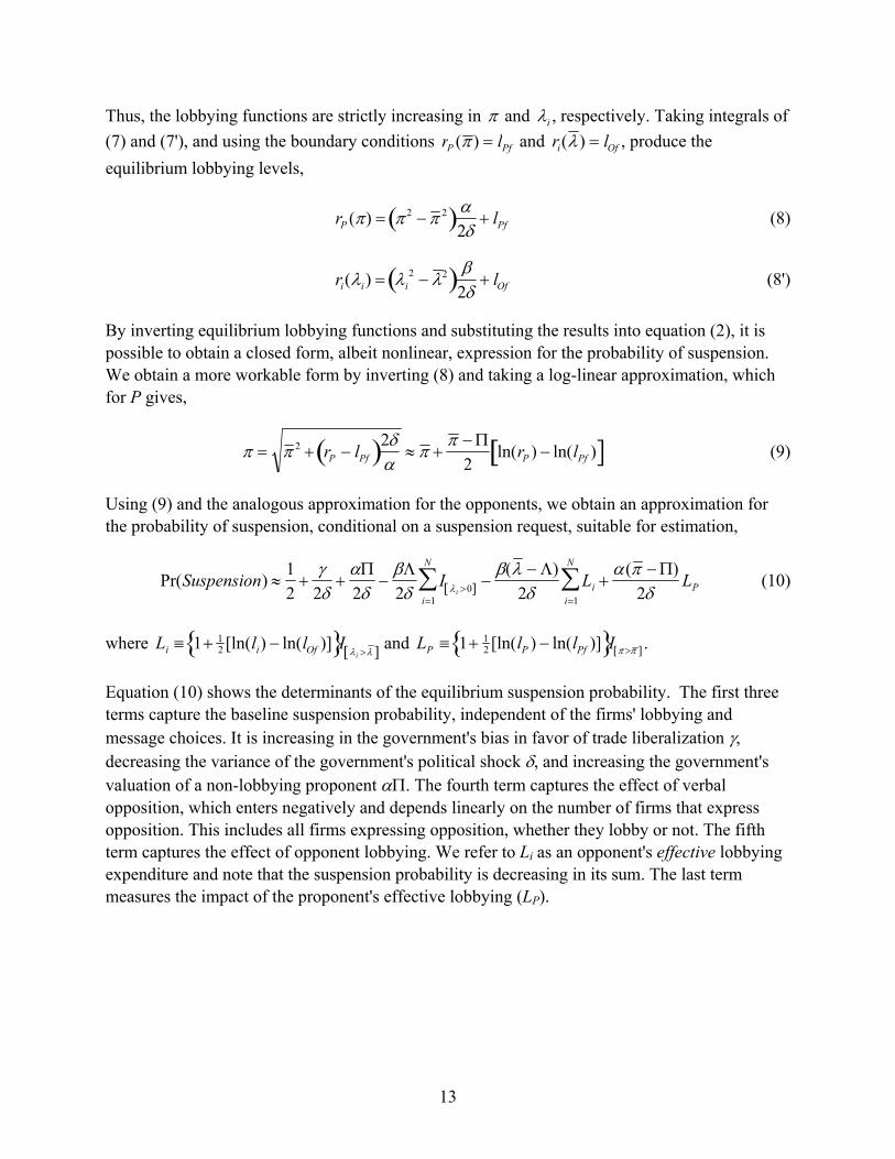
Thus, the lobbying functions are strictly increasing in and i , respectively. Taking integrals of

(7) and (7'), and using the boundary conditions rP () lPf and ri() lOf , produce the

equilibrium lobbying levels,

rP () 2 2 2

lPf (8)

ri(i) i2 2

2 lOf (8')

By inverting equilibrium lobbying functions and substituting the results into equation (2), it is possible to obtain a closed form, albeit nonlinear, expression for the probability of suspension. We obtain a more workable form by inverting (8) and taking a log-linear approximation, which for P gives,

2 rP lPf 2

2ln(rP ) ln(lPf ) (9)

Using (9) and the analogous approximation for the opponents, we obtain an approximation for the probability of suspension, conditional on a suspension request, suitable for estimation,

Pr(Suspension) 1

2

22

2

I i 0 i1

N

( )

2Li

i1

N

()

2LP (10)

where Li 1 12 [ln(li) ln(lOf )] I i and LP 1 1

2 [ln(lP ) ln(lPf )] I .

Equation (10) shows the determinants of the equilibrium suspension probability. The first three terms capture the baseline suspension probability, independent of the firms' lobbying and message choices. It is increasing in the government's bias in favor of trade liberalization , decreasing the variance of the government's political shock , and increasing the government's valuation of a non-lobbying proponent . The fourth term captures the effect of verbal opposition, which enters negatively and depends linearly on the number of firms that express opposition. This includes all firms expressing opposition, whether they lobby or not. The fifth term captures the effect of opponent lobbying. We refer to Li as an opponent's effective lobbying expenditure and note that the suspension probability is decreasing in its sum. The last term measures the impact of the proponent's effective lobbying (LP).

14

Equations (8) and (10) are illustrated in figures 1 and 2, which show the lobbying functions and corresponding suspension probabilities as functions of the firms' payoffs. In figure 1a, proponent lobbying equals zero for and increases quadratically for . Corresponding to this, figure 1b shows that probability of suspension jumps at , which is the point at which the proponent begins to lobby and government revises upwards its expectation of , and increases linearly in thereafter. Figures 2a and 2b show similar patterns for each opponent. The difference is that at i 0 the opponent does not verbally oppose the suspension, while for i 0 it does. This causes a downward jump in the probability of suspension at i 0 in figure

2b, followed by a second downward jump at i as the opponent starts to lobby.

Figure 1a. Proponent lobbying function Figure 1b. Suspension probability as function of

Figure 2a. Opponent lobbying function Figure 2b. Suspension probability as function of i

ii

No Opposition

No Opposition

lOf

lPf

15

IV. DATA

In this section we first provide background information on tariff suspensions. Next, we describe the dataset on lobbying expenditures and compare it with contributions from Political Action Committees (PACs). Finally, we present summary statistics for the main variables used in the empirical analysis.

A. Tariff suspensions

The data on tariff suspensions is collected from two sources: the USITC bill reports on each proposed tariff suspension and the U.S. Harmonized Tariff Schedule maintained by the USITC. In each Congress, representatives and senators propose tariff suspension bills on behalf of various proponent firms. The bills address very specific products. For example, in the 109th Congress, Senator DeMint sponsored a bill on behalf of proponent firm Michelin to eliminate the tariff on “sector mold press machines to be used in production of radial tires designed for off-the-highway use with a rim measuring 63.5 cm or more in diameter” (S. 2219). Once the tariff bills are referred by formal memorandum to the House Ways and Means Committee or the Senate Finance Committee, the USITC compiles a report on the bill. This study focuses on the 106th (1999-2000), 107th (2001-2002), 108th (2003-2004), and 109th (2005-2006) Congresses.

USITC produces a separate report for every suspension bill introduced in each Congress.17 The reports include information about the proponent firm, estimates of expected tariff revenue loss, dutiable imports, and current tariff rates.18 To gain information about firm opposition, the USITC sends questionnaires to possible producers and purchasers of the good in question. From the responses to the questionnaires, the USITC notes if the firms are current/future producers of the product (106th and 107th Congress) or whether they oppose the tariff suspension bill (108th and 109th Congress).

In particular, the bill report format changes throughout the time period in question. For the 106th and the 107th Congress bill reports, the USITC indicates whether surveyed firms submitted responses and, based on these responses, it indicates whether there is any domestic current/future production of the product. Economic intuition suggests that a domestic producer would be opposed to the bill, as they would not want to compete with a cheaper imported product. Therefore, for the 106th and 107th Congresses (about 25% of our total sample), we assume that firms indicating current/future domestic production oppose the suspension. In the 108th and the 109th Congress, the reports change slightly and include direct information on whether specific firms voiced opposition to the measure. We use this information to construct our opposition variable for the latter two Congresses. Finally, note that information in the reports about domestic production of the good or domestic opposition to the bill is dependent upon the responses provided by surveyed firms, many of which do not respond. Non-response suggests

17 The bill reports are posted on the ITC website http://www.usitc.gov/tariff_affairs/congress_reports/. 18 See Figure B1 for an example of a USITC bill report prepared for the 109th Congress.

16

that the firms are not sufficiently opposed to the legislation to expend the resources necessary to reply to the USITC. Thus we classify non-response cases as no opposition cases.

To ascertain whether the tariff suspension bills have been enacted into law, we use the U.S. Harmonized Tariff Schedule (HTS). Each product on which a suspension is granted is removed from its normal eight-digit HTS product category and assigned a temporary eight-digit number, beginning with 99, and listed in Chapter 99 of the HTS. This chapter is updated annually. We therefore search Chapter 99 in the years following the passage of a Miscellaneous Tariff Bill (MTB) to determine which suspension bills were successful. If the product specified in a suspension bill is not found, we assume the bill failed.

Congress generally passes the trade bills in the form of a single MTB for each congress. The 106th Congress enacted two bills into law, the Miscellaneous Trade and Technical Corrections Act of 1999 (H.R. 435) and the Trade Suspensions Act of 2000 (H.R. 4868). Therefore, we use the HTS for 2002 to check which bills passed. The 107th Congress did not successfully pass an MTB. Instead, the bills from that Congress were rolled into the Miscellaneous Trade and Technical Correction Act of 2004 (H.R. 1047) and passed by the 108th Congress. All of the bills in the 107th Congress addressed different products from ones introduced in the 108th Congress. Therefore, we did not have to worry about duplicative bills spanning the two Congresses. We use the HTS of 2006 for these two Congresses.

Finally, we use the HTS of 2008 for the 109th Congress. Although the Miscellaneous Trade and Technical Act of 2006 never became law, most of the duty suspensions can be found at the end of the Tax Relief and Health Care Act of 2006 (H.R. 6111), which did become law.

B. Lobbying expenditures

We use a novel dataset on lobbying expenditures at the firm level in order to construct a measure of the payments firms make to influence tariff suspensions. We compile the dataset using the websites of the Center for Responsive Politics (CRP) and the Senate’s Office of Public Records (SOPR), which provide information on semi-annual lobbying disclosure reports. We use data from the reports covering lobbying activity that took place from 1999 through 2006.

With the introduction of the Lobbying Disclosure Act of 1995, individuals and organizations have been required to provide a substantial amount of information on their lobbying activities at the Federal level.19 Starting from 1996, all lobbyists had to file semi-annual reports to the Secretary of the SOPR, listing the name of each client (firm) and the total income they have received from each of them. At the same time, all firms with in-house lobbying departments are required to file similar reports stating the total dollar amount (i.e., both for in-house and outside lobbying) they have spent. Importantly, legislation requires the disclosure not only of the total

19 According to the Lobbying Disclosure Act of 1995, the term lobbying activities refers to lobbying contacts and efforts in support of such contacts, including preparation and planning activities, research and other background work that is intended, at the time it is performed, for use in contacts, and coordination with the lobbying activities of others.

17

dollar amounts actually received/spent, but also of the issues for which lobbying is carried out. Table B1 shows a list of 76 general issues at least one of which has to be entered by the filer. The report filed by a firm producing chemicals, 3M Company, for the period January-June 2006, is shown in Figure B2. The firm spent $985,000 over the specified period in lobbying activities. The federal agencies contacted by the firm include the Department of Commerce and the Office of the US Trade Representative. It lists “trade” as an issue it lobbies for. Importantly, it also lists “duty suspension” as a specific issue with which the lobbying activities are associated. 20

Annual lobbying expenditures and incomes (of lobbying firms) are calculated by adding mid-year and year-end totals. The lobbying expenditures of a firm associated with issues relevant to the tariff suspension bills are calculated using a two-step procedure. First, we consider those firms that list trade or any other issue pertaining to the bills in their lobbying report.21 In particular, the list of 76 general issues specified by the SOPR, which a firm has to choose from when it files its lobbying report (see Table B1), includes some of the industries affected by the tariff suspensions (for example, chemical and textiles).22 Therefore, a firm lobbying policymakers in favor or against the tariff suspension might write down “trade” in its lobbying report or, alternatively, “chemical”, textile”, etc. Second, we split the total expenditure of each firm equally between the issues they lobbied for and consider the fraction accounted for by trade or any other issue pertaining to the bills. So for example, if the firm lobbies on six issues, which include, among others, trade and chemical – then we use one third of the firm’s total lobbying expenditure.

Finally, we merge information on each tariff suspension bill’s proponent and opponent firms with the firm-level dataset on lobbying expenditures. We sum each firm-level lobbying expenditures over the two years that Congress was in session. We assume that, if a (proponent or opponent) firm is not in the lobbying dataset, then the firm did not make any lobbying expenditures. Thus, merging the tariff suspension and lobbying datasets allows us to clearly distinguish firms that spend money to lobby on issues related to tariff suspensions from those that do not. Henceforth, we shall refer to a firm that makes positive lobbying expenditures specifically on trade or other issues related to the bill as politically "organized", while those that do not are "unorganized."23

20 Unfortunately the reports do not give information on how the total dollar amount spent by a firm (or received by a lobbying company) is split across different general issues. Therefore, we will assume that issues receive equal weight. 21 The lobbying dataset from 1999-2006 comprises an unbalanced panel of a total of 15,310 firms/associations of firms, out of which close to 30% list trade or any other issue pertaining to the bills. 22 The majority of the bills (close to 70%) address chemical products. Beyond chemicals, bills address a wide spectrum of intermediate goods, including but not limited to fabrics and fibers, shoes, airplane parts, bicycle parts, camcorders, foodstuff, and sports equipment. The list of lobbying issues other than trade which we classify as pertaining to the bills are (i) chemicals (ii) mining (iii) food (iv) manufacturing (v) textiles and (vi) transport. 23 In the Grossman-Helpman model, the term “organized” refers to sector represented by a lobby that makes contributions on behalf of all firms in the sector, thus implying collective action among firms. Our definition of organized differs in that it refers to an individual firm that spends money on lobbying, with no presumption of

18

C. Comparison between lobbying expenditures and PAC contributions

In addition to carrying out lobbying activities, special interest groups in the United States can legally influence the policy formation process by offering campaign finance contributions. As pointed out before, PAC contributions have been the focus of the bulk of the quid pro quo literature. In an information model, the distinction between lobbying and contributions is unimportant. The reasons we focus primarily on lobbying expenditures in our empirical work is that they are quantitatively the most important form of political spending, and, unlike PAC contributions, can be disaggregated by issue.

Given the existing limits on their size, PAC contributions are not the most important route by which interest groups' money can influence policy makers.24 Milyo, Primo, and Groseclose (2000) point out that lobbying expenditures are of “... an order of magnitude greater than total PAC expenditure.” Between 1999 and 2006, interest groups spent on average about 4.2 billion U.S. dollars per political cycle on targeted political activity, which includes lobbying expenditures and PAC campaign contributions.25 Lobbying expenditures represent close to ninety percent of all targeted political expenditure.

Figure 3 shows the relationship between lobbying expenditures for trade and related issues and PAC contributions by firm. It is based on averages over the four election cycles. We see that while some firms that make PAC contributions do not lobby, it is far more common that lobbying firms do not make PAC contributions. For those firms doing both, we find a very high and positive correlation between the two modes of political spending.26

collective action. As an empirical matter, organization is always measured on the basis of spending. Thus, our definition is operationally equivalent to that of previous sector-level studies; only the unit of observation is different. 24 PACs can give $5,000 to a candidate committee per election (primary, general or special). They can also give up to $15,000 annually to any national party committee, and $5,000 annually to any other PAC (source: http://www.opensecrets.org/pacs/pacfaq.php). 25 We follow the literature that excludes from targeted-political-activity soft money contributions, which went to parties for general party-building activities not directly related to federal campaigns; in addition, soft money contributions cannot be associated with any particular interest or issue (see Milyo, Primo, and Groseclose 2000 and Tripathi, Ansolabehere, and Snyder 2002). Soft money contributions have been banned by the 2002 Bipartisan Campaign Reform Act. 26 This is in contrast to Facchini, Mayda and Mishra (2008) who find zero correlation between PAC contributions and lobbying expenditures on immigration at the sector level.

19

Figure 3. Scatter Plots between Lobbying Expenditures and Campaign Contributions from Political Action Committees (PACs) at the Firm Level

Campaign contributions from PACs and lobbying expenditures on trade and other issues related to tariff suspension bills

(in millions of US$)

Notes. The scatter plots are based on data on campaign contributions and lobbying expenditures over four election cycles -- 1999-2000, 2001-02, 2003-04 and 2005-06. The correlation between (log) contributions from PACs and (log) lobbying expenditures for trade is 0.504 (robust standard error=0.041; p-value=0.000). Logarithms of zero values of PAC and lobbying expenditures are assumed equal to zero.

05

10

15

20

PA

C c

on

trib

utio

ns b

y f

irm

s (

in lo

gs)

0 5 10 15 20Lobbying expend itures on trade and related issues by firms (in logs)

Although our empirical work relies mainly on lobbying expenditures, for robustness, we also create a broader measure of each firm’s political organization, which includes both lobbying expenditures (on trade and other issues related to the bill) and PAC campaign contributions. Each PAC is sponsored by a firm (or a group of firms) so we can identify campaign contributions for each firm. Data on PAC contributions at the firm level comes from the website of the Center of Responsive Politics (http://www.opensecrets.org/pacs/list.php).

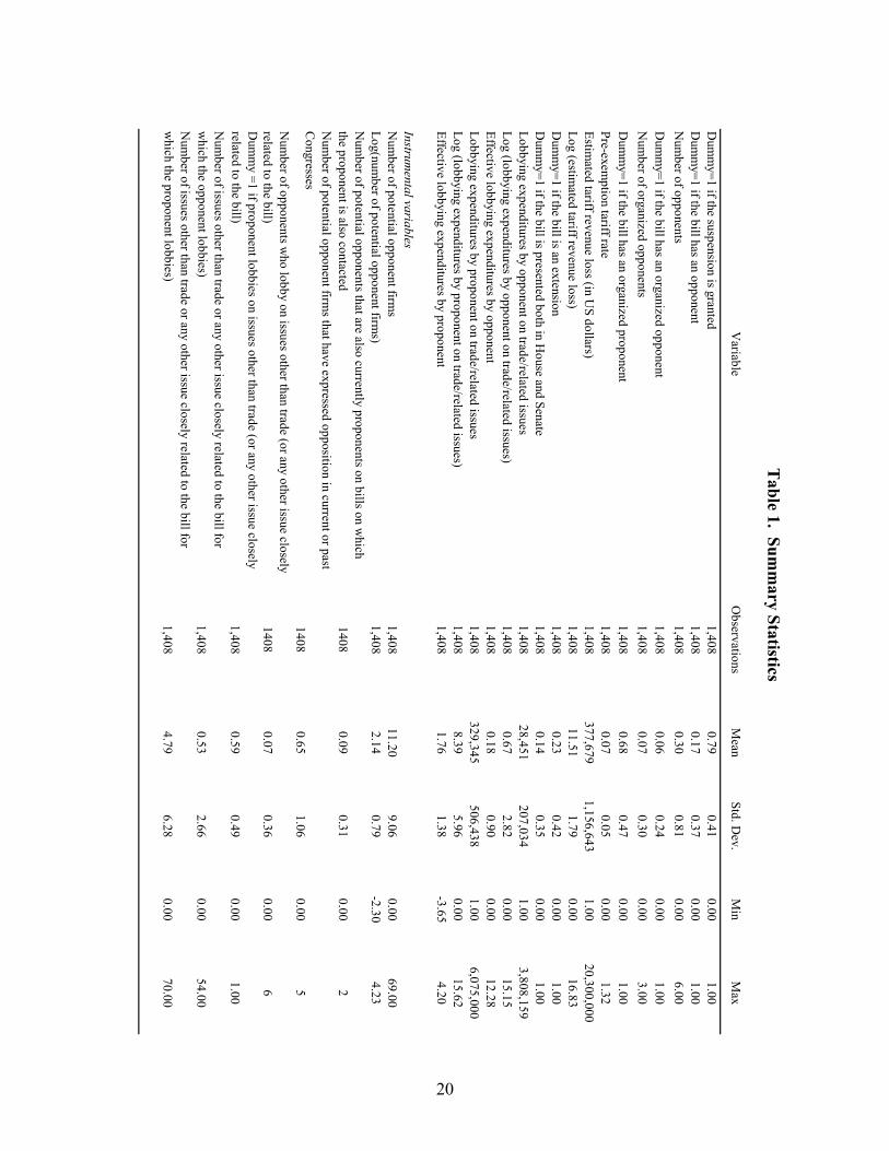
D. Summary Statistics

Summary statistics of the main variables used in the empirical analysis are presented in Table 1. The data shows that Congress passes tariff suspensions more often than not: 79% of the tariff suspension bills are passed. Therefore, the proponents have a fairly high success rate on bill passage. The fraction of bills with at least one opponent firm is quite low (17%). However, among bills with opponents, multiple opponents are fairly common. Roughly half of the bills

20

have more than one opponent.27 In addition, 23% of the bills seek to extend previously passed tariff suspensions, and 14% of the bills are submitted more than once during a given Congress, i.e. the same proponent firm submits the bill to both the House and the Senate.28 Finally, the average tariff rate applied to products for which suspension is requested is 7%, which is near the average applied MFN tariff rate for all dutiable U.S. imports.29

27 In contrast, only 3% of the bills have more than one proponent. Therefore, in the theoretical model, we assumed a single proponent and multiple opponents at the bill-level. 28 There are also (rare) cases in which two different proponent firms submit different bills on the same product. 29 In 2006, the final year of our data, the simple average applied MFN tariff rate on all items (using tariff-line averaging with HS 2002 base) was 4.5%, while on dutiable imports it was 7.6%. The difference is caused by the fact that over a third of U.S. tariff lines were duty free. Source: WTO Integrated Data Base.

20

Tab

le 1. Su

mm

ary Statistics

Variable

Observations

Mean

Std. D

ev.M

inM

ax

Dum

my=

1 if the suspension is granted1,408

0.790.41

0.001.00

Dum

my=

1 if the bill has an opponent1,408

0.170.37

0.001.00

Num

ber of opponents1,408

0.300.81

0.006.00

Dum

my=

1 if the bill has an organized opponent1,408

0.060.24

0.001.00

Num

ber of organized opponents1,408

0.070.30

0.003.00

Dum

my=

1 if the bill has an organized proponent1,408

0.680.47

0.001.00

Pre-exem

ption tariff rate1,408

0.070.05

0.001.32

Estim

ated tariff revenue loss (in US

dollars)1,408

377,6791,156,643

1.0020,300,000

Log (estim

ated tariff revenue loss)1,408

11.511.79

0.0016.83

Dum

my=

1 if the bill is an extension1,408

0.230.42

0.001.00

Dum

my=

1 if the bill is presented both in House and S

enate1,408

0.140.35

0.001.00

Lobbying expenditures by opponent on trade/related issues

1,40828,451

207,0341.00

3,808,159L

og (lobbying expenditures by opponent on trade/related issues)1,408

0.672.82

0.0015.15

Effective lobbying expenditures by opponent

1,4080.18

0.900.00

12.28L

obbying expenditures by proponent on trade/related issues1,408

329,345506,438

1.006,075,000

Log (lobbying expenditures by proponent on trade/related issues)

1,4088.39

5.960.00

15.62E

ffective lobbying expenditures by proponent1,408

1.761.38

-3.654.20

Instrumental variables

Num

ber of potential opponent firms

1,40811.20

9.060.00

69.00L

og(number of potential opponent firm

s)1,408

2.140.79

-2.304.23

Num

ber of potential opponents that are also currently proponents on bills on which

the proponent is also contacted1408

0.090.31

0.002

Num

ber of potential opponent firms that have expressed opposition in current or past

Congresses

14080.65

1.060.00

5N

umber of opponents w

ho lobby on issues other than trade (or any other issue closely related to the bill)

14080.07

0.360.00

6D

umm

y =1 if proponent lobbies on issues other than trade (or any other issue closely

related to the bill)1,408

0.590.49

0.001.00

Num

ber of issues other than trade or any other issue closely related to the bill for w

hich the opponent lobbies)1,408

0.532.66

0.0054.00

Num

ber of issues other than trade or any other issue closely related to the bill for w

hich the proponent lobbies)1,408

4.796.28

0.0070.00

21

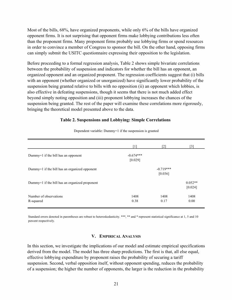
Most of the bills, 68%, have organized proponents, while only 6% of the bills have organized opponent firms. It is not surprising that opponent firms make lobbying contributions less often than the proponent firms. Many proponent firms probably use lobbying firms or spend resources in order to convince a member of Congress to sponsor the bill. On the other hand, opposing firms can simply submit the USITC questionnaire expressing their opposition to the legislation.

Before proceeding to a formal regression analysis, Table 2 shows simple bivariate correlations between the probability of suspension and indicators for whether the bill has an opponent, an organized opponent and an organized proponent. The regression coefficients suggest that (i) bills with an opponent (whether organized or unorganized) have significantly lower probability of the suspension being granted relative to bills with no opposition (ii) an opponent which lobbies, is also effective in defeating suspensions, though it seems that there is not much added effect beyond simply noting opposition and (iii) proponent lobbying increases the chances of the suspension being granted. The rest of the paper will examine these correlations more rigorously, bringing the theoretical model presented above to the data.

Table 2. Suspensions and Lobbying: Simple Correlations

[1] [2] [3]

Dummy=1 if the bill has an opponent -0.674***[0.029]

Dummy=1 if the bill has an organized opponent -0.719***[0.036]

Dummy=1 if the bill has an organized proponent 0.052**[0.024]

Number of observations 1408 1408 1408R-squared 0.38 0.17 0.00

Standard errors denoted in parentheses are robust to heteroskedasticity. ***, ** and * represent statistical significance at 1, 5 and 10 percent respectively.

Dependent variable: Dummy=1 if the suspension is granted

V. EMPIRICAL ANALYSIS

In this section, we investigate the implications of our model and estimate empirical specifications derived from the model. The model has three sharp predictions. The first is that, all else equal, effective lobbying expenditure by proponent raises the probability of securing a tariff suspension. Second, verbal opposition itself, without opponent spending, reduces the probability of a suspension; the higher the number of opponents, the larger is the reduction in the probability

22

of suspension. Third, effective lobbying expenditures by the opponents decrease the probability of the suspension.

A. Empirical Strategy

Our estimation is based on equation (10). To begin, we abstract from the lobbying expenditure levels and consider only the effects of political organization. This simplification allows for comparison with the quid pro quo literature, which takes this approach. The regression equation is specified as follows:

, ,, 0 , 1 , 2 , 3 , ,Pr( 1) opp org opp org prop

i t i t i t i t i t s t i tSuspension a N N D Z v (11)

where i and t denote the bill and Congress, respectively, and s denotes the HTS section.30

Pr(Suspension 1) is the probability that the suspension requested in the bill is granted; ,oppi tN is

the number of opponent firms for bill i ; ,,org oppi tN is the number of politically organized

opponents, i.e. the number of opponent firms which lobby on trade or any other issue pertaining

to the bill; proporgtiD ,, is a dummy which is equal to 1 if the proponent firm of the bill is politically

organized, i.e. it lobbies on trade or any other issue pertaining to the bill. ,i tZ denotes the vector

of additional controls at the bill-congress level. The control variables include the pre-suspension tariff rate, the (log of the) estimated tariff revenue loss, a dummy which is equal to 1 if the bill is an extension of a previous bill, and a dummy which is equal to 1 if the bill is presented both in the House and Senate. In addition, we also include political variables – a dummy which is equal to 1 if the sponsor belongs to the House Ways and Means or Senate Finance Committees in the current or past three Congresses and a dummy equal to 1 if the sponsor belongs to the Democratic Party. All regressions include HTS section and Congress fixed effects (denoted, respectively, by s and t ). Finally, we also include interactions between party of the sponsor

and Congress fixed effects to control for additional political variables, e.g. whether the sponsor belongs to the same party as the chairman of Senate Finance and House Ways and Means committees, whether the sponsor belongs to the majority party in the Congress. Equation (11) is estimated using a linear probability model.31

The parameters of interest are 0 , 1 and 2 . In terms of equation (10), we can interpret these

parameters as 0 /2 0, 1 ( )LO /2 0 and 2 ()LP /2 0. In this specification, we treat the level of effective lobbying expenditures of each opponent ( LO ) and proponent ( LP ) as part of the parameter to be estimated. Variation in effective lobbying

30 Notice that, in Equation (11), the political organization of opponents is measured by the number of organized opponents, while that for the proponents is measured by a dummy. This reflects the fact that bills with multiple opponents are fairly common whereas multiple proponents are rare (Section 4.4 for details). 31 The results in the paper are robust to estimating Equation (11) by probit. However, we prefer the linear probability model since fixed-effects estimation of a probit model may lead to inconsistent estimates, due to the so called incidental parameter problem (Chamberlain 1984).

23

expenditures, both across observations and across individual opponents for the same observation, is ignored.

In our second specification, we estimate Equation (10), explicitly accounting for variation in the levels of lobbying expenditures of the proponents and opponents. The regression equation is specified as follows:

Pr(Suspension 1)i,t a 0N i,topp 1SLi,t

opp 2Li,tprop 3Zi,t s vt i,t (12)

where Li,tprop denotes the effective lobbying expenditures by the proponent for trade or other

issues related to the bill, and SLi,topp denotes the sum of effective lobbying expenditures for

organized opponents. Recall from equation (10) that the effective lobbying expenditures depend on (logs of) the minimum feasible lobbying expenditures lPf and lOf . Note that these values are

assumed to be constant across bills and firms of the same type. Thus, as proxies for lPf and lOf ,

we choose the minimum lobbying expenditures in the data, over all firms and bills, for the proponents and opponents, respectively. In this specification, the coefficients correspond to the theory according to: 0 /2 0, 1 ( ) /2 0 and 2 () /2 0.

Endogeneity is an issue for both regressions (11) and (12). All three of our main variables, N i,t

opp , N i,torg,opp , Di,t

org,prop in regression (11) and N i,topp, SLi,t

opp , Li,tprop in regression (12), could be

endogenous due to reverse causality. For example, if the ex-ante expected probability of suspension is high – for some reason we do not account for in the right-hand-side of the equation – potential opponent firms may decide not to come forward and oppose the bill, expecting a small impact of their opposition and, at the same time, not wanting to incur the cost of opposition (for instance, a potential opponent might wish to avoid provoking retaliation from the proponent, in the event that their roles are reversed on another bill). Similarly, if the probability of success of a bill is high, opponent firms may decide it is not worthwhile to invest (or to invest a lot) in lobbying expenditures to try to block it. These reverse-causality effects would imply a negative correlation between the unobserved component of the probability of suspension and N i,t

opp,N i,torg,opp , SLi,t

opp ; hence, they would exaggerate the magnitude of the (negative) estimated

effects.32 Finally, the decision of a proponent firm to invest (and how much) in lobbying expenditures could also be related to expectations regarding its probability of suspension, and bias the estimated coefficients on Di,t

org,prop and Li,tprop .

To address the endogeneity problems described above, we use an instrumental variables strategy.

We use three different instruments for the number of opponents ( opptiN , ). First, we construct a

variable intended to capture the dependence of potential opponents on the proponent.

32 However, the same type of argument may work in the opposite direction, i.e. upstream firms may be more inclined to come forward and oppose the bill and invest in lobbying expenditures when they fear that the suspension is more likely to be granted. This case is not problematic for us since our estimates of 0 , 1 and0 , 1 would be biased towards zero, i.e. they would be a lower bound of the true negative effects.

24

Specifically, we measure the number of potential opponent firms contacted for the bill in question, say, bill X, that are also currently proponents on other bills for which the proponent of bill X is a potential opponent. The idea underlying the instrument is that the opponents are likely to cooperate with proponents when they have something to lose in the current period. Hence, when the value of this instrument is higher, we expect a smaller number of opponents (first stage). The second instrument is the number of potential opponent firms that have expressed opposition in past (or current) Congresses. We expect that, the higher is this number, the higher should be the number of opponents (first stage). In other words, we assume that certain firms have expertise or are more accustomed to expressing opposition; thus, if a bill has a larger number of contacted firms that have expressed opposition in the past, it is likely to have larger a number of opponents in the current period. Finally, the third instrument is the number of firms contacted by the ITC.33 The higher is this number, the higher the number of actual opponents is likely to be, for the following two reasons: first, if all potential opponents have some chance of actually opposing, then the more potential opponents there are the higher the expected number of actual opponents; second, and most importantly, in a market with several domestic producers, it will be harder for the proponent firm to buy them off – i.e. convince them not to come forward – for example in a situation of collusion. Therefore, we expect the number of contacted firms to be

positively correlated with the endogenous regressor opptiN , (first-stage).

The three instruments are unlikely to be correlated with the unobserved component of the probability of suspension, i.e. they are unlikely to have a direct effect on the latter probability. What is relevant from the point of view of decision makers is whether the bill negatively impacts upstream domestic firms, which is the case only if the latter ones say so by voicing their opposition. It is unlikely that the success of the bill depends on the instruments independently from whether the tariff suspension is opposed (exclusion restriction). For example, the dependence of potential opponents on the proponent is likely to have an effect on the passage of the bill only through its effect on opposition. To conclude, the three instruments plausibly allow

us to address the endogeneity of opptiN , .

To construct instruments for the number of politically organized opponent firms ( N i,torg,opp ) and

whether the proponent firm is politically organized ( Di,torg,prop), we use firm-level data on lobbying

activity. In particular, for each firm which spends lobbying money on trade or other issues related to the bill, we consider whether or not it lobbies for other issues, i.e. issues unrelated to the bill e.g. defense. We use as instruments the number of opponents who lobby on unrelated issues and a dummy equal to 1 if the proponent lobbies on unrelated issues. A firm which lobbies for unrelated issues is likely to have overcome many of the fixed costs associated with lobbying, and thus it would be easier for the firm to channel lobbying money to influence decisions regarding the tariff suspension bill. Thus, we expect to find strong first-stage relationships. At the same time, there is no reason why the lobbying activity of the firm on unrelated issues should

33 Note that the lists of contacted firms are compiled by ITC staff who are not close to the top of the hierarchy, hence are not likely to be related to decisions made by the Congress regarding the passage of the bills.

25

have a direct impact on the probability of passage of the tariff suspension (exclusion restriction). Thus, the number (indicator) of opponent (proponent) firm lobbying on unrelated issues plausibly allows us to address endogeneity. Finally, for the measure of effective lobbying expenditures ( SLi,t

opp, Li,tprop ) , we use as instruments the number of unrelated issues the opponent

firms and the proponent firm lobby for, respectively.34

Besides endogeneity, another possible source of concern is that we observe only suspension bills that are introduced into Congress. We cannot speak to the determinants of introduction, because it is not possible to observe bills not introduced. Economic intuition, however, would suggest that proponents refrain from introducing bills that are doomed to failure, and thus the 79% raw success rate in our sample is not representative of all conceivable bills. How problematic this is depends in large measure on the scope of the question being addressed. Both our theory and empirical strategy are designed to capture the effect of lobbying and verbal opposition on the success rate of bills that have been, and, under the current regime, are likely to be, introduced into Congress. We believe this to be the most relevant question, and our estimates are valid in this context.35

B. OLS benchmark results

We first estimate the model using ordinary least squares. Table 3 presents our main results. We find a strong, negative and significant (at the 1% level) impact of opposition on the probability of passage of the tariff suspension bill. This result is robust across specifications; in particular it is not affected by whether we measure political organization using a discrete or a continuous variable (compare columns (1)-(2) to columns (3)-(4)).

34 Recall that the lobbying reports do not provide the split of total lobbying expenditures among various issues and we derive lobbying expenditures on unrelated issues also from the total expenditures. In order to avoid a mechanical correlation between the instrument and the regressor, we do not use the expenditures on unrelated issues as instrument. 35 If we were interested in the wider population of all potential bills (i.e., those introduced and those not introduced), additional complications could arise. If the proponent’s decision to introduce a bill is a function of exogenous observables, such as the tariff rate or the number of potential opponents, selection does not give rise to a bias in the estimates of the coefficients (Wooldridge, 2002). If the introduction of bills is systematically correlated with unobservables that affect the probability of the suspension being granted, then selection bias could occur. As we do not have any information on the bills that are not introduced, it is impossible to implement any of the usual corrections for sample selection. Therefore, we focus our attention only to the subpopulation of bills that are introduced and will refrain from drawing any conclusions for the wider population.

26

Table 3. Suspensions and Lobbying: Ordinary Least Squares

[1] [2] [3] [4]

Number of opponents -0.176*** -0.176*** -0.195*** -0.195***

[0.030] [0.029] [0.030] [0.029]

Number of organized opponents -0.251*** -0.256***

[0.072] [0.073]

Dummy=1 if the bill has an organized proponent 0.027 0.011

[0.021] [0.022]

Effective lobbying expenditures by opponent -0.062** -0.063**

[0.025] [0.025]

Effective lobbying expenditures by proponent 0.018** 0.014*

[0.007] [0.008]

Pre-exemption tariff rate 0.227* 0.251* 0.213 0.234*

[0.137] [0.147] [0.132] [0.138]

Estimated tariff revenue loss (in logs) -0.002 -0.003

[0.005] [0.005]

Dummy=1 if the bill is an extension 0.074*** 0.073***

[0.020] [0.020]

Dummy=1 if the bill is presented both in House and Senate 0.060** 0.057*

[0.030] [0.030]

Dummy=1 if sponsor belongs to the House Ways and Means or Senate Finance Committees in the current or past three Congresses 0.039 0.03

[0.025] [0.025]

Dummy=1 if sponsor belongs to the Democratic Party 0.024 0.025

[0.059] [0.060]

Dummy=1 if Congress=107 0.154*** 0.166*** 0.156*** 0.168***

[0.039] [0.040] [0.039] [0.040]

Dummy=1 if Congress=108 0.005 0.064 0.008 0.062

[0.059] [0.072] [0.059] [0.071]

Dummy=1 if Congress=109 0.123*** 0.129*** 0.121*** 0.125***

[0.028] [0.034] [0.028] [0.034]

Number of observations 1408 1408 1408 1408

R-squared 0.31 0.32 0.30 0.31

Standard errors denoted in parentheses are robust to heteroskedasticity. ***, ** and * represent statistical significance at 1, 5 and 10 percent respectively. Effective lobbying expenditures=1+[Log (lobbying expenditures)-minimum Log (lobbying expenditures)]/2. All regressions include industry fixed effects and interaction between the Congress fixed effects and party of the sponsor.

Dependent variable: Dummy=1 if the suspension is granted

27

Note that the estimate of the coefficient of N i,topp (i.e.,0) captures the impact of firms that oppose

suspension but do not lobby, since the regression equation controls for opporgtiN

,, . More precisely,

all else equal, each unorganized opponent firm decreases probability of suspension by 0 . The fact that 0 is negative and significant is not consistent with the model of Grossman and Helpman (1994). That model predicts that a product with unorganized domestic producers should actually receive less protection than products with no domestic producers at all. In fact they should receive a negative tariff, or an import subsidy. In the case of tariff suspension bills, a zero tariff is the lower bound. So, if we interpret firms that express opposition without spending to be unorganized producers and those that do not express opposition to be nonproducers, we would expect that the effect of opposition sans lobbying would be to increase the likelihood of a suspension being granted. In contrast, according to our estimate in column (1), each unorganized opponent reduces the probability of suspension by roughly 17.6 percentage points. Therefore, tariff suspensions do not fit well into a pure quid pro quo model. Rather, they are consistent with

our model of informational lobbying. The coefficient of ,oppi tN can be interpreted to measure the

impact of cheap talk. The fact that it is negative and significant tells us that simply noting opposition does impact the passage of a bill.

Our results also show that ,,org oppi tN – the political organization of the opponent firm(s) – is

effective at reducing the likelihood that the tariff suspension passes. This estimate is significant at the 1% level, using either the discrete measure or the level of effective lobbying expenditures. The coefficient 1 on organized opposition (-25.1 percentage points in column (1)) captures the additional effect – above and beyond the impact of unorganized opposition – of opponent lobbying on the probability of the legislation’s passage. Therefore, a bill with one firm noting opposition, that also lobbies, is 42.7 percentage points less likely to pass. The coefficient of

,,org oppi tN can be interpreted as a measure of the impact of costly lobbying. The finding that it is

negative and statistically significant suggests that costly lobbying by opponents is effective in reducing the bill’s passage. The findings are similar if we use effective lobbying expenditures by opponent instead of the discrete variable (columns (3) and (4)). As predicted by the theoretical model, higher effective lobbying expenditure by opponents reduces the probability of the suspension being passed. The estimated effect is statistically significant at the 5 percent level.36 As argued above, it is difficult to disentangle the motives for lobbying based on political spending. Hence either (both) the information channel, which is the focus of this paper, or (and) the quid pro quo channel could be driving this result.

On the proponent side, columns (1) and (2) show no significant impact of political organization by the proponent firm. However, when we use the continuous lobbying variable (which is more consistent with the estimating equation derived from the theory), we do find that higher

36 Note that Effective lobbying expenditures=constant+[Log (lobbying expenditures)]/2. Therefore, the estimates in column (3) and (4) suggest that a one percent rise in actual lobbying expenditures by opponents reduces the chances of passage of bill by about 3 percentage points.

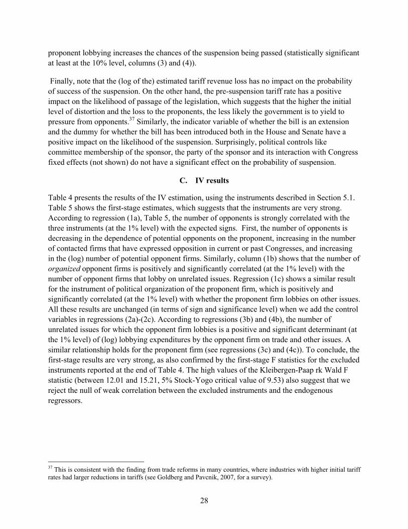
28

proponent lobbying increases the chances of the suspension being passed (statistically significant at least at the 10% level, columns (3) and (4)).

Finally, note that the (log of the) estimated tariff revenue loss has no impact on the probability of success of the suspension. On the other hand, the pre-suspension tariff rate has a positive impact on the likelihood of passage of the legislation, which suggests that the higher the initial level of distortion and the loss to the proponents, the less likely the government is to yield to pressure from opponents.37 Similarly, the indicator variable of whether the bill is an extension and the dummy for whether the bill has been introduced both in the House and Senate have a positive impact on the likelihood of the suspension. Surprisingly, political controls like committee membership of the sponsor, the party of the sponsor and its interaction with Congress fixed effects (not shown) do not have a significant effect on the probability of suspension.

C. IV results

Table 4 presents the results of the IV estimation, using the instruments described in Section 5.1. Table 5 shows the first-stage estimates, which suggests that the instruments are very strong. According to regression (1a), Table 5, the number of opponents is strongly correlated with the three instruments (at the 1% level) with the expected signs. First, the number of opponents is decreasing in the dependence of potential opponents on the proponent, increasing in the number of contacted firms that have expressed opposition in current or past Congresses, and increasing in the (log) number of potential opponent firms. Similarly, column (1b) shows that the number of organized opponent firms is positively and significantly correlated (at the 1% level) with the number of opponent firms that lobby on unrelated issues. Regression (1c) shows a similar result for the instrument of political organization of the proponent firm, which is positively and significantly correlated (at the 1% level) with whether the proponent firm lobbies on other issues. All these results are unchanged (in terms of sign and significance level) when we add the control variables in regressions (2a)-(2c). According to regressions (3b) and (4b), the number of unrelated issues for which the opponent firm lobbies is a positive and significant determinant (at the 1% level) of (log) lobbying expenditures by the opponent firm on trade and other issues. A similar relationship holds for the proponent firm (see regressions (3c) and (4c)). To conclude, the first-stage results are very strong, as also confirmed by the first-stage F statistics for the excluded instruments reported at the end of Table 4. The high values of the Kleibergen-Paap rk Wald F statistic (between 12.01 and 15.21, 5% Stock-Yogo critical value of 9.53) also suggest that we reject the null of weak correlation between the excluded instruments and the endogenous regressors.

37 This is consistent with the finding from trade reforms in many countries, where industries with higher initial tariff rates had larger reductions in tariffs (see Goldberg and Pavcnik, 2007, for a survey).

29

Table 4. Suspensions and Lobbying: Instrumental Variables Regressions

[1] [2] [3] [4]

Number of opponents -0.130** -0.121** -0.138*** -0.133***[0.055] [0.055] [0.049] [0.049]

Number of organized opponents -0.283*** -0.292***[0.102] [0.101]

D=1 if bill has an organized proponent 0.063** 0.056*[0.028] [0.029]

Effective lobbying expenditures by opponent -0.064** -0.063**[0.031] [0.031]

Effective lobbying expenditures by proponent 0.041*** 0.040***[0.011] [0.011]

Pre-exemption tariff rate 0.264* 0.287** 0.257* 0.268*[0.143] [0.146] [0.138] [0.139]

Eestimated tariff revenue loss (in logs) -0.004 -0.006[0.005] [0.006]

Dummy=1 if the bill is an extension 0.077*** 0.077***[0.020] [0.021]

Dummy=1 if the bill is presented both in House and Senate 0.055* 0.049[0.030] [0.030]

Dummy=1 if sponsor belongs to the House Ways and Means or Senate Finance Committees in the current or past three Congresses 0.029 0.013

[0.025] [0.025]

Dummy=1 if sponsor belongs to the Democratic Party 0.035 0.044[0.060] [0.062]

Dummy=1 if Congress=107 0.169*** 0.184*** 0.180*** 0.198***[0.040] [0.041] [0.041] [0.041]

Dummy=1 if Congress=108 0.008 0.052 0.023 0.058[0.058] [0.070] [0.057] [0.068]

Dummy=1 if Congress=109 0.132*** 0.134*** 0.135*** 0.131***

[0.028] [0.034] [0.028] [0.033]Number of observations 1408 1408 1408 1408R-squared 0.22 0.23 0.20 0.21Instrumental variables

First-stage F (number of opponents) 24.56 25.53 20.16 21.1First-stage F (number of organized opponents) 30.95 27.90First-stage F (D=1 if bill has an organized proponent) 284.27 276.26First-stage F (effective lobbying expenditures by opponent) 32.46 33.03First-stage F (effective lobbying expenditures by proponent) 97.07 85.53Hansen's J statistic (p value) 0.44 0.38 0.75 0.63Standard errors denoted in parentheses are robust to heteroskedasticity. ***, ** and * represent statistical significance at 1, 5 and 10 percent respectively. The first-stage regressions are shown in Table 5. The number of opponents; number of organized opponents; dummy for organized proponent; and the effective lobbying expendituresof opponents and proponents, are treated as endogenous. Effective lobbying expenditures=1+[Log (lobbying expenditures)-minimum Log (lobbying expenditures)]/2. All regressions include industry fixed effects and interaction between the Congress fixed effects and party of the sponsor.

Number of opponents who lobby on issues other than trade (or any other issue closely related to the bill)

Number of issues other than trade or any other issue closely related to the bill for which the opponent lobbies

Number of potential opponent firms that have expressed opposition in cuurent or past Congresses

Number of issues other than trade or any other issue closely related to the bill for which the proponent lobbies

Dummy =1 if proponent lobbies on issues other than trade (or any other issue closely related to the bill)

Number of potential opponent firms that have expressed opposition in cuurent or past Congresses

Dependent variable: Dummy=1 if the suspension is granted

Number of potential opponent firms (in logs) Nnumber of potential opponent firms (in logs)

Number of potential opponents that are also currently proponents on bills on which the proponent is also contacted

Number of potential opponents that are also currently proponents on bills on which the proponent is also contacted

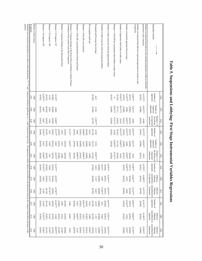
30

[1a][1b]

[1c][2a]

[2b][2c]

[3a][3b]

[3c][4a]

[4b][4c]

Dependent variable:

Num

ber of opponents

Num

ber of organized opponents

Dum

my=

1 if the bill has

an organized proponent

Num

ber of opponents

Num

ber of organized opponents

Dum

my=

1 if the bill has an

organized proponent

Num

ber of opponents

Effective

lobbying expenditures by opponent

Effective

lobbying expenditures by

proponent

Num

ber of opponents

Effective

lobbying expenditures by

opponent

Effective

lobbying expenditures by

proponent

Num

ber of contacted firms that are also currently proponents on bills on w

hich the proponent is also contacted

-0.113***-0.032***

-0.006-0.127***

-0.034***-0.012

-0.174***-0.090***

0.357***-0.191***

-0.100***0.298***

[0.027][0.008]

[0.015][0.027]

[0.009][0.017]

[0.031][0.021]

[0.079][0.030]

[0.022][0.080]

Num

ber of contacted firms that have expressed opposition in cuurent or past

Congresses

0.082***0.012**

-0.0070.073***

0.011**-0.012

0.100***0.043***

-0.167***0.095***

0.042***-0.179***

[0.017][0.005]

[0.010][0.017]

[0.005][0.010]

[0.017][0.016]

[0.028][0.017]

[0.016][0.028]

Num

ber of potential opponent firms (in logs)

0.223***0.008

0.022**0.231***

0.0090.029**

0.209***-0.027

0.0480.216***

-0.0220.075*

[0.032][0.008]

[0.011][0.032]

[0.008][0.011]

[0.032][0.022]

[0.043][0.032]

[0.023][0.044]

Num

ber of opponents which lobby on other issues

0.836***0.671***

-0.0330.813***

0.669***-0.033

[0.182][0.111]

[0.029][0.181]

[0.112][0.028]

Dum

my=

1 if the bill has a proponent which lobbies on other issues

00.033***

0.727***-0.038

0.028***0.725***

[0.037][0.009]

[0.020][0.041]

[0.010][0.020]

Num

ber of other issues for which the opponent lobbies

0.079***0.283***

-0.074***0.077***

0.282***-0.075***

[0.026][0.027]

[0.015][0.026]

[0.027][0.015]

Nnum

ber of other issues for which the proponent lobbies

0.012**0.007

0.148***0.01

0.0060.145***

[0.006][0.004]

[0.009][0.006]

[0.004][0.009]

Estim

ated tariff revenue loss (in logs)-0.42

0.326-1.055***

-0.3020.336

-0.983***-0.421

1.151*-0.627

-0.3471.193

-0.313

[0.285][0.206]

[0.159][0.318]

[0.217][0.162]

[0.304][0.696]

[0.395][0.339]

[0.729][0.423]

Pre-exem

ption tariff rate0.013

-0.002-0.008

0.0160.008

0.030**

[0.010][0.002]

[0.005][0.010]

[0.007][0.015]

Dum

my=

1 if the bill is an extension-0.080**

-0.0140.060***

-0.091***-0.027

0.157**

[0.031][0.009]

[0.022][0.033]

[0.023][0.063]

Dum

my=

1 if the bill is presented both in House and S

enate0.003

0.024*0.098***

0.0130.082**

0.124

[0.053][0.014]

[0.026][0.054]

[0.041][0.079]

Dum

my=

1 if sponsor belongs to the House W

ays and Means or Senate F

inance C

omm

ittees in the current or past three Congresses

0.112**0.035**

-0.037**0.086

0.066*0.076

[0.053][0.014]

[0.018][0.054]

[0.035][0.068]

Dum

my=

1 if sponsor belongs to the Dem

ocratic Party

-0.0170.027

-0.0090.001

0.034-0.256*

[0.072][0.021]

[0.048][0.066]

[0.072][0.149]

Dum

my=

1 if Congress=

107-0.118**

-0.004-0.069**

-0.113**0.007

-0.073**-0.167***

-0.074**-0.756***

-0.144***-0.049

-0.897***

[0.046][0.009]

[0.028][0.047]

[0.012][0.033]

[0.051][0.034]

[0.094][0.053]

[0.035][0.103]

Dum

my=

1 if Congress=

108-0.101

0.023-0.04

0.050.045

0.03-0.066

0.127*-0.334***

0.0530.156*

-0.350**

[0.073][0.022]

[0.032][0.107]

[0.032][0.027]

[0.076][0.067]

[0.125][0.114]

[0.091][0.155]

Dum

my=

1 if Congress=

109-0.226***

0.0070.021

-0.141**0.027

0.050**-0.193***

0.0390.109

-0.103*0.102***

0.204**

[0.043][0.013]

[0.021][0.058]

[0.018][0.024]

[0.038][0.029]

[0.074][0.053]

[0.038][0.087]

Num

ber of observations1408

14081408

14081408

14081408

14081408

14081408

1408

R-squared

0.410.69

0.590.42

0.690.61

0.360.75

0.500.37

0.750.52

Standard errors denoted in parentheses are robust to heteroskedasticity. ***, ** and * represent statistical significance at 1, 5 and 10 percent respectively. A

ll regressions include industry fixed effects and interaction between the C

ongress fixed effects and party of the sponsor.

Tab

le 5. Su

spen

sions an

d L

obb

ying: F

irst Stage In

strum

ental V

ariables R

egressions

31

The second-stage results confirm most of the OLS results. Both unorganized and organized opposition have a negative and significant impact on the likelihood of passage of the tariff suspension bill. In addition, proponent firm’s political organization now has a positive and significant impact, as predicted by the theoretical model. All these findings are confirmed when we use the level of effective lobbying expenditures to measure the extent of political organization of opponent and proponent firms. The magnitude of the estimated coefficients on organized proponents is much higher in the IV regressions compared to the OLS. For example, in regression (1) of Table 4, a bill with an organized proponent is more than twice as likely to pass (compared to Table 3). The direction of the bias suggests a negative correlation between the unexplained probability of suspension and proponent lobbying in the OLS regressions. In other words, bills with a higher ex-ante expected probability of suspension are likely to be associated with a lower degree of proponent political organization. Finally, the results on the control variables are qualitatively unchanged.

To summarize the results, both the OLS and the instrumental variable regressions confirm the key predictions of the theoretical model: (i) verbal opposition itself, without lobbying, reduces the probability of suspension, (ii) greater political organization or higher lobbying expenditures by the proponent is associated with a higher probability of suspension and (iii) greater political organization or higher lobbying expenditures by the opponent, though relatively rare, is effective at defeating the suspension.

D. Robustness checks: broader measures of political organization

As mentioned in Section 4.1, lobbying expenditures represent the bulk of total targeted political activity (accounting for up to 90% of it) with the remaining portion (only approximately 10%) being made up by PAC campaign contributions. In addition, as shown in Figure 3, at the firm level, lobbying expenditures (on trade and other issues related to the bill) and PAC contributions are positively and significantly correlated. Thus, we believe that by using lobbying expenditures data we are accounting for most of the variation in lobbying activity. However, to check the robustness of our results, we also use firm-level data on PAC campaign contributions, which allows us to fully control for the impact of lobbying activity. We create a broader measure of political organization where a bill is defined to have a politically organized opponent (proponent) if the opponent (proponent) makes either lobbying expenditures on trade or related issues or PAC contributions, or both.38 In other words, the key difference between this table and Tables 3 and 4 is that cheap talk is defined more strictly as a situation in which the opponents voice their verbal opposition without spending on lobbying expenditures nor on PAC contributions. The estimates are shown in Table 6. The main result – that cheap talk reduces the probability of suspension – continues to hold strongly in most specifications. As in Tables 3 and 4, political organization of opponents (proponents) reduces (increases) significantly the probability of suspension.

38 According to the broader definition of political organization, 106 and 21 additional bills have politically organized proponents and opponents, respectively.

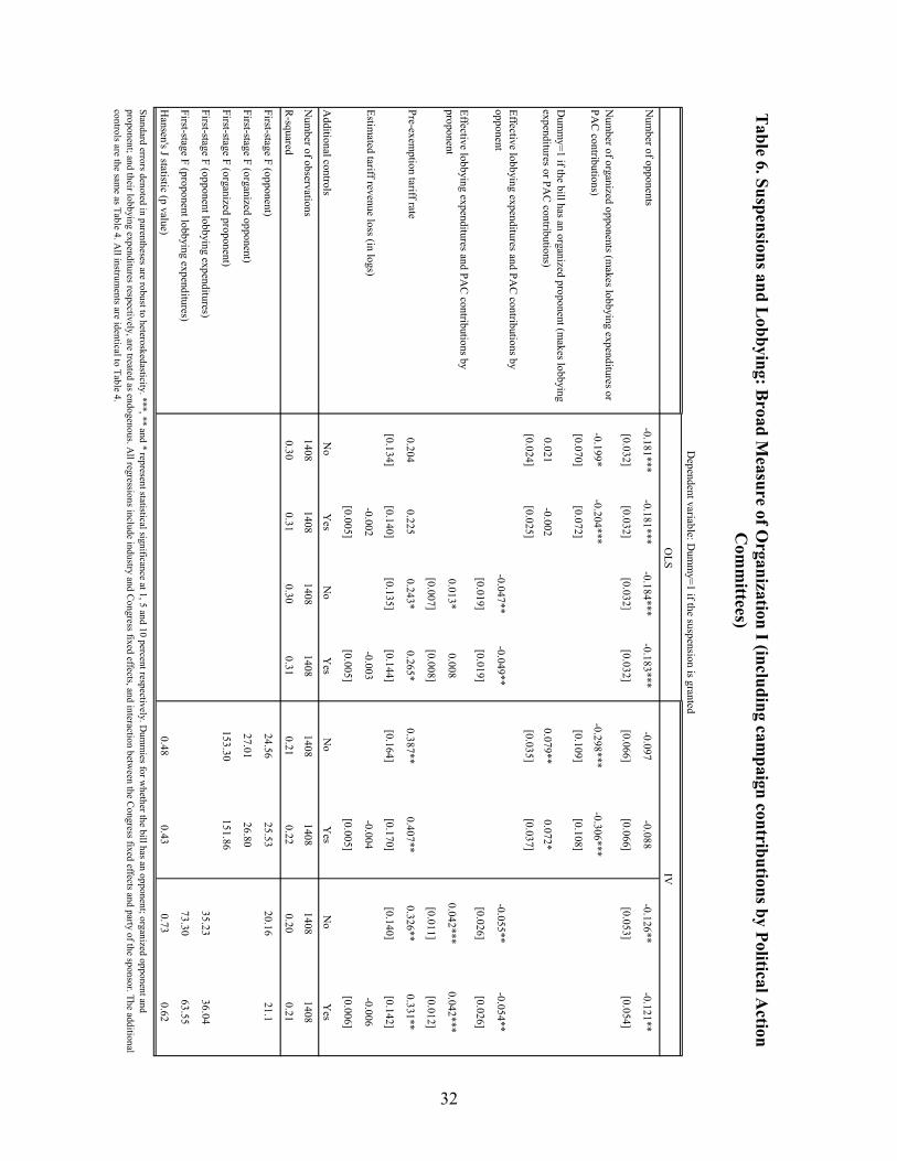
32

Num

ber of opponents-0.181***

-0.181***-0.184***

-0.183***-0.097

-0.088-0.126**

-0.121**

[0.032][0.032]

[0.032][0.032]

[0.066][0.066]

[0.053][0.054]

Num

ber of organized opponents (makes lobbying expenditures or

PA

C contributions)

-0.199*-0.204***

-0.298***-0.306***

[0.070][0.072]

[0.109][0.108]

Dum

my=

1 if the bill has an organized proponent (makes lobbying

expenditures or PA

C contributions)

0.021-0.002

0.079**0.072*

[0.024][0.025]

[0.035][0.037]

Effective lobbying expenditures and P

AC

contributions by opponent

-0.047**-0.049**

-0.055**-0.054**

[0.019][0.019]

[0.026][0.026]

Effective lobbying expenditures and P

AC

contributions by proponent

0.013*0.008

0.042***0.042***

[0.007][0.008]

[0.011][0.012]

Pre-exem

ption tariff rate0.204

0.2250.243*

0.265*0.387**

0.407**0.326**

0.331**

[0.134][0.140]

[0.135][0.144]

[0.164][0.170]

[0.140][0.142]

Estim

ated tariff revenue loss (in logs)-0.002

-0.003-0.004

-0.006

[0.005][0.005]

[0.005][0.006]

Additional controls

No

Yes

No

Yes

No

Yes

No

Yes

Num

ber of observations1408

14081408

14081408

14081408

1408

R-squared

0.300.31

0.300.31

0.210.22

0.200.21

First-stage F

(opponent)24.56

25.5320.16

21.1

First-stage F

(organized opponent)27.01

26.80

First-stage F

(organized proponent)153.30

151.86

First-stage F

(opponent lobbying expenditures)35.23

36.04

First-stage F

(proponent lobbying expenditures)73.30

63.55

Hansen's J statistic (p value)

0.480.43

0.730.62

Dependent variable: D

umm

y=1 if the suspension is granted

OL

SIV

Standard errors denoted in parentheses are robust to heteroskedasticity. ***, ** and * represent statistical significance at 1, 5 and 10 percent respectively. D

umm

ies for whether the bill has an opponent; organized opponent and

proponent; and their lobbying expenditures respectively, are treated as endogenous. All regressions include industry and C

ongress fixed effects, and interaction between the C

ongress fixed effects and party of the sponsor. The additional

controls are the same as T

able 4. All instrum

ents are identical to Table 4.

Tab

le 6. Su

spen

sions an

d L

obb

ying: B

road M

easure of O

rganization

I (inclu

din

g camp

aign con

tribu

tions b

y Political A

ction

Com

mittees)

33

Another concern is that although firms note opposition without spending money in the current period, they could be making promises about spending money in future periods; alternatively, they could have already made the expenditures in previous Congresses. Hence noting verbal opposition in the current period without spending may not be an accurate measure of cheap talk. In order to address this concern, we define political organization more broadly to include lobbying expenditure in the past, current and future Congresses. The results are reported in Table 7. Again, noting opposition without spending money in the past, current or future, reduces significantly the probability of suspension. Political organization of the opponent is effective in reducing the probability of suspension, whereas political organization of the proponent increases the probability of suspension.

34

Num

ber of opponents-0.172***

-0.171***-0.196***

-0.195***-0.125**

-0.118**-0.129**

-0.125**

[0.029][0.029]

[0.030][0.030]

[0.058][0.057]

[0.051][0.051]

Num

ber of organized opponent in current, past or future Congresses

-0.243***-0.252***

-0.292***-0.305***

[0.071][0.070]

[0.099][0.097]

Dum

my=

1 if the bill has an organized proponent in current, past or future C

ongresses0.01

-0.010.028

0.013

[0.022][0.023]

[0.027][0.028]

Effective lobbying expenditures by opponent in current, past and future

Congresses

-0.060**-0.062**

-0.079**-0.080**

[0.027][0.027]

[0.033][0.034]

Effective lobbying expenditures by proponent in current, past and future

Congresses

0.016**0.011

0.050***0.050***

[0.008][0.008]

[0.012][0.013]

Pre-exemption tariff rate

0.243*0.266*

0.219*0.242*

0.287*0.310**

0.307**0.320**

[0.139][0.152]

[0.132][0.139]

[0.148][0.155]

[0.142][0.143]

Additional controls

No

Yes

No

Yes

No

Yes

No

Yes

Num

ber of observations1408

14081408

14081408

14081408

1408

R-squared

0.310.32

0.300.31

0.220.24

0.190.20

First-stage F (opponent)27.82

28.7122.81

23.68

First-stage F

(organized opponent)58.21

52.37

First-stage F

(organized proponent)961.83

858.01

First-stage F (opponent lobbying expenditures)54.79

56.55

First-stage F (proponent lobbying expenditures)100.92

90.12

Hansen's J statistic (p value)

0.260.20

0.910.84

Standard errors denoted in parentheses are robust to heteroskedasticity. ***, ** and * represent statistical significance at 1, 5 and 10 percent respectively. E

ffective lobbying expenditures=1+

[Log (lobbying expenditures)-

minim

um L

og (lobbying expenditures)]/2. The num

ber of opponents; number of organized opponents; dum

my for organized proponent; and the effective lobbying expendituresof opponents and proponents, are treated as

endogenous. All regressions include industry and C

ongress fixed effects, and interaction between the C

ongress fixed effects and party of the sponsor. The additional controls are the sam

e as Table 4. T

he instruments are the sam

e as in T

ables 4 and 6, except those for organization and effective lobbying expenditures, which are redefined to include past, current and future C

ongresses.

Dependent variable: D

umm

y=1 if the suspension is granted

OL

SIV

T

able 7. S

usp

ension

s and

Lob

byin

g --Broad

Measu

re of Organ

ization II (in

clud

ing lob

byin

g in p

ast and

futu

re Con

gresses)

35

To conclude, the main results in the paper continue to hold strongly if we include broader measures of political organization to include (i) PAC contributions and (ii) lobbying expenditures in the past and future Congresses. 39, 40

VI. CONCLUSIONS

We have developed a model that incorporates information as a driver of trade policy. We found that verbal opposition itself, without opponent spending, reduces the probability of a suspension, as does trade policy lobbying by organized opponents. Additionally, trade policy lobbying by organized proponents increases probability of a suspension. We have empirically tested these predictions using data on US tariff suspensions and firm-level information on trade lobbying expenditures. Our results are consistent with theory and are robust to addressing endogeneity concerns using an IV estimation strategy.

We began with the question of whether lobbying expenditures constitute quid pro quo or a signal of information, and we have provided a partial answer. Our estimates give the first systematic empirical evidence that “cheap talk,” in the form of costless signaling of opposition to trade liberalization, has an impact on trade policy. The finding that cheap talk is influential implies that the government relies on information possessed by firms; if this is so, it follows from the model that political spending must also convey information. That said, we cannot rule out the possibility that lobbying expenditures are also a form of quid pro quo, as quid pro quo spending is observationally equivalent to signaling in our model. Thus, while the exact mixture of signaling and quid pro quo cannot be distinguished, we do find that information matters and so does spending. Moreover, we have achieved a substantial improvement in accuracy over previous work in the estimation of the spending effect by clearly linking targeted lobbying expenditures to discretionary tariff changes, using firm level data.

39 We also check the robustness of our results to dropping bills that are extensions to previous bills. The results are unaffected. 40 Another possible concern is that firms that oppose without spending money might be able to convince policymakers to do what is best for them because these firms receive the support of a large number of voters (and not because these firms credibly convey information about what is good for the policymakers). In other words, policymakers do not want to penalize firms that, for example, employ many workers or are very visible in the local economy. In order to address this concern, we control for the number of employees in each opponent firm by merging our dataset with data from Compustat. Since Compustat includes only publicly listed firms, our sample size reduces drastically by half. Controlling for the number of employees of the opponent firm, we still find that conveying information without spending money continues to reduce significantly the probability of suspension (in the OLS specifications). In order to avoid losing observations, we also estimate a regression including instead of the number of employees, a dummy for whether the firm is in Compustat, to denote an indicator variable for large firms. The results are qualitatively similar.

36

References

Austen-Smith, David, 1992, “Strategic Models of Talk in Political Decision Making,” International Political Science Review, Vol. 13, No. 1, pp. 45-58.

Austen-Smith, David and John Wright, 1994, “Counteractive Lobbying,” American Journal of

Political Science, Vol. 38, No. 1, pp. 25-44. Bagwell, Kyle and Robert W. Staiger, 2009, "What Do Trade Negotiators Negotiate About?

Empirical Evidence from the World Trade Organization," American Economic Review, forthcoming.

Bohara, Alok K and William H. Kaempfer, 1991, “A Test of Tariff Endogeneity in the United

States,” American Economic Review, Vol. 81, No. 4, pp. 952-60. Bombardini, Matilde and Francesco Trebbi, 2009, “Competition and Political Organization:

Together or Alone in Lobbying for Trade Policy?,” NBER working paper No. 14771 (Cambridge, Massachusetts: National Bureau of Economic Reseach)

Broda, Christian, Nuno Limao, and David E. Weinstein, 2008, "Optimal Tariffs and Market

Power: The Evidence," American Economic Review, Vol. 98, No. 5, pp. 2032–65. Chamberlain, G., 1984. Panel data. In: Griliches, Z., Intriligator, M.D. (Eds.), Handbook of

Econometrics, Vol. 2. (North-Holland, Amsterdam). Chen, Hui, David C. Parsley, and Ya-wen Yang, 2010, “Corporate Lobbying and Financial

Performance.” Available via the Internet: http://ssrn.com/abstract=1014264. Costinot, Arnaud, 2009, “Jobs, Jobs, Jobs: A 'New' Perspective on Protectionism,” Journal of the

European Economic Association, Vol. 7 No. 5, pp. 1-31. de Figueiredo, John M. and Charles M. Cameron, 2009, “Endogenous Cost Lobbying: Theory

and Evidence,” CELS 2009 4th Annual Conference on Empirical Legal Studies Paper. Available via the Internet: http://ssrn.com/abstract=1443559.

de Figueiredo, J. M. and B. S. Silverman, 2006, “The Returns to Lobbying: University Lobbying

Efforts and the Allocation of Earmarked Academic Grants,” Journal of Law and Economics, Vol. 49, pp. 597-626.

Ederington, Josh and Jenny Minier, 2008, “Reconsidering the Empirical Evidence on the

Grossman-Helpman Model of Endogenous Protection,” Canadian Journal of Economics, Vol. 41, No. 3, pp. 501-516.

Eicher, Theo and Thomas Osang, 2002, “Protection for Sale: An Empirical Investigation: A

Comment,” American Economic Review, Vol. 92, No. 5, pp. 1702-11.

37

European Union, 1998, “Commission communication concerning autonomous tariff suspensions and quotas,” Official Journal of the European Communities (98/C 128/02).

Facchini, Giovanni, Anna Maria Mayda, and Prachi Mishra, 2008. “Do Interest Groups Affect

US Immigration Policy?,” CEPR Discussion Paper No. DP6898. Gawande, Kishore and Usree Bandyopadhyay, 2000, “Is Protection for Sale? Evidence on the

Grossman-Helpman Theory of Endogenous Protection,” Review of Economics and Statistics, Vol. 82, No. 1, pp. 139-152.

Gawande, Kishore, Pravin Krishna, and Marcelo Olarreaga, 2005, “Lobbying Competition Over

Trade Policy,” NBER Working Paper No. 11371. Gawande, Kishore, Pravin Krishna, and Michael J Robbins, 2006, “Foreign Lobbies and U.S.

Trade Policy,” Review of Economics and Statistics, Vol. 88, No. 3, pp. 563-571. Gawande, Kishore, William Maloney, and Gabriel Montes-Rojas, 2009, “Foreign informational

lobbying can enhance tourism: Evidence from the Caribbean,” Journal of Development Economics, Vol. 90, No. 2, pp. 267-275.

Goldberg, Pinelopi Koujianou and Giovanni Maggi, 1999, “Protection for Sale: An Empirical

Investigation,” American Economic Review, Vol. 89, No. 5, pp. 1135-1155. Goldberg, Pinelopi Koujianou and Nina Pavcnik, 2007, “Distributional Effects of Globalization

in Developing Countries,” Journal of economic Literature, Vol. 45, No. 1, pp. 39-82. Grossman, Gene M. and Elhanan Helpman, 1994, “Protection for Sale,” American Economic

Review, Vol. 84, No. 4, 833-850. Grossman, Gene M. and Elhanan Helpman, 2001, Special Interest Politics, (Boston: MIT Press). ———, 2005, “A Protectionist Bias in Majoritarian Politics,” Quarterly Journal of Economics,

Vol. 120, No. 4, pp. 1239-1282. Gokcekus, Omer and Amber Barth, 2007, “Political economy of the U.S. temporary duty

suspension program: An empirical note,” Public Choice, Vol. 131, pp. 345-350. Imai, Susumu, Hajime Katayama, and Kala Krishna, 2009, “Is Protection Really for Sale?

Survey and Directions for Future Research,” International Review of Economics & Finance, Vol. 18, No. 2, pp. 181-191.

Lohmann, Susanne, 1995, “Information, Access and Contributions: A Signaling Model of

Lobbying,” Public Choice, Vol. 85, pp. 267-284. Ludema, Rodney D. and Anna Maria Mayda, 2008, “Do Countries Free Ride on MFN?” Journal

of International Economics, Vol. 77, No. 2, pp. 137-150.

38

———, 2010 “Do Terms of Trade Effects Matter for Trade Agreements? Evidence from WTO

Countries,” CEPR Discussion Paper 7695. Mansfield, Edward D. and Marc L. Busch, 1995, “The Political Economy of Nontariff Barriers:

A Cross-National Analysis,” International Organization, Vol. 49, No. 4, pp. 723-749. Mayer, Wolfgang, 1984, “Endogenous Tariff Formation,” American Economic Review, Vol. 74,

No. 5, pp. 970-985. Milyo, Jeffrey, David Primo, and Timothy Groseclose, 2000, “Corporate PAC Campaign

Contributions in Perspective,” Business and Politics, Vol. 2, No. 1, pp. 75-88. Potters, Jan. and Frans van Winden, 1992, “Lobbying and asymmetric information,” Public

Choice, Vol. 74, pp. 269–292. Pinsky, Laura and Edward Tower, 1995, “Temporary duty suspension in the United States,”

North American Journal of Economics and Finance, Vol. 6, No. 1, pp. 17–36. Dutt, Pushan and Devashish Mitra, 2002, “Endogenous trade policy through majority voting: an

empirical investigation,” Journal of International Economics, Vol. 58, No. 1, pp: 107–133.

Snyder, J. M., 1990, “Campaign Contributions as Investments: The US House of Representatives

1908-1986,” Journal of Political Economy, Vol. 61, pp. 195-206. Trefler, D., 1993, “Trade Liberalization and the Theory of Endogenous Protection: An

Econometric Study of U.S. Import Policy,” Journal of Political Economy, Vol. 101, pp. 138-160.

Tripathi, M., S. Ansolabehere, and J. Snyder, 2002, “Are PAC Contributions and Lobbying

linked? New Evidence from the 1995 Lobby Disclosure Act.” Business and Politics, Vol 4: 131-155.

Wooldridge, J. M., 2002, Econometric analysis of cross section and panel data, (Cambridge,

Massachusetts: MIT Press) Wright, John R., 1996, Interest Groups and Congress: Lobbying, Contributions, and Influence

(Boston: Allyn & Bacon)

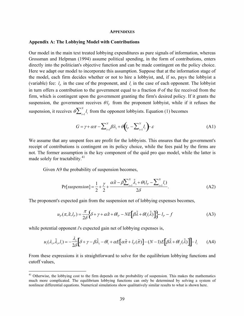
39

APPENDIXES

Appendix A: The Lobbying Model with Contributions

Our model in the main text treated lobbying expenditures as pure signals of information, whereas Grossman and Helpman (1994) assume political spending, in the form of contributions, enters directly into the politician's objective function and can be made contingent on the policy choice. Here we adapt our model to incorporate this assumption. Suppose that at the information stage of the model, each firm decides whether or not to hire a lobbyist, and, if so, pays the lobbyist a (variable) fee: lP in the case of the proponent, and li in the case of each opponent. The lobbyist

in turn offers a contribution to the government equal to a fraction of the fee received from the firm, which is contingent upon the government granting the firm's desired policy. If it grants the suspension, the government receives lP from the proponent lobbyist, while if it refuses the

suspension, it receives lii1

N from the opponent lobbyists. Equation (1) becomes

G ii1

N lP lii1

N (A1)

We assume that any unspent fees are profit for the lobbyists. This ensures that the government's receipt of contributions is contingent on its policy choice, while the fees paid by the firms are not. The former assumption is the key component of the quid pro quo model, while the latter is made solely for tractability.41

Given A9 the probability of suspension becomes,

Pr[suspension] 1

22 ˜ ˜ ii1

N (lP lii1

N )

2. (A2)

The proponent's expected gain from the suspension net of lobbying expenses becomes,

uP (, ˜ , lP ) 2

˜ lP NE ˜ li(˜ ) lP f (A3)

while potential opponent i's expected gain net of lobbying expenses is,

ui(i, ˜ i, li) i

2 ˜ i li E ˜ lP ( ˜ ) (N 1)E ˜ l j ( ˜ ) li (A4)

From these expressions it is straightforward to solve for the equilibrium lobbying functions and cutoff values,

41 Otherwise, the lobbying cost to the firm depends on the probability of suspension. This makes the mathematics much more complicated. The equilibrium lobbying functions can only be determined by solving a system of nonlinear differential equations. Numerical simulations show qualitatively similar results to what is shown here.

40

rP () 2 2 2

l f (A5)

ri(i) i2 2

2 l f (A6)

2

2 l f (A7)

Thus, the only effect of adding contingent contributions to the government's objective function is to increase the aggressiveness of lobbying. Qualitatively, however, the model is unchanged.

41

Appendix B

A Model of Vertical Production with Wage Rigidity

The model in the main text assumed reduced forms payoffs to the firms and the government. Here we show a complete economic model to justify those reduced forms. We assume that the proponent and opponents are adjacent links in a vertical production chain. To produce a unit of good Y the proponent combines, in fixed proportions, one unit of good X, which may be imported at a fixed price p = p* + t, and one unit of an input QP, which the proponent produces using land, labor and firm-specific capital, according to the Cobb-Douglas production function, QP KP

1TP(1 )LP

. The proponent receives a fixed price a for each unit of Y sold. Similarly, to produce a unit of good X, each opponent combines, in fixed proportions, one unit of an intermediate input Z, which can be acquired at firm-specific cost bi, with one unit of input Qi, produced using land, labor and firm-specific capital, according to the Cobb-Douglas production function, Qi Ki

1Ti(1 )Li

. Assuming the wage is fixed at w and the land rent normalized is to

1, the minimum cost of quantities QP and Qi are AwQP1/KP

(1 ) / and BwQi1/Ki

(1 ) / ,

respectively, where A (1)1 and B (1 )1 . Setting KP Ki 1 and 12 , we can

write firm profits as functions of Y and X as follows,

P (a p)YP AwYP2 (B1)

i (p b)Xi Bw Xi2 (B2)

Maximizing A1 givesYP (a p) / Aw , P (a p)2 /4Aw and LP P /w , for the output, profit and employment, respectively, of the proponent. Maximizing A2 gives the corresponding values of each opponent: Xi (p bi) /Bw , i (p bi)

2 /4Bw , and Li i /w .

Assume the economy is endowed with L workers, and those not working one of the N+1 firms receive an outside wage of 1. We assume w > 1, possibly due to union wage bargaining, efficiency wages, or some other labor market distortion specific to the sector. The effect of the tariff suspension on welfare thus depends the change in labor income, the changes in producer profits and the loss of tariff revenue (there is no change in consumer surplus, as the price of Y is fixed). Thus,

W w 1

w

i

i1

N

i

i1

N

i

(p p) Y Xi

i1

N

(B3)

The first term in B3 reflects the wage distortion and the fact that changes in employment are proportional to changes in profits. The gain to the proponent and loss the opponent can be written,

42

(p p)(2a p p)

Aw (B4)

i ( p p)( p p 2bi)

Bw (B5)

If we think of a and bi as being privately observed by the proponent and opponents, respectively, then and i are private information. Substituting A4-A5 into A3 and simplifying gives,

W 1

Aw 1

Bw

t 2

4 w 1

w

w 1

w

ii1

N (B6)

Defining the first term in B6 as , we see it is a function of the squared tariff and is thus

proportional the dead-weight loss of the tariff. The coefficients on the second and third terms in A6 correspond to and respectively. These are constants that depend on the size of the wage

distortion. This is why the wage distortion (or some other distortion) is a necessary part of the story if we want to interpret G solely in welfare terms.

43

Table B1. List of Issues

Code Issue ACC Accounting ADV Advertising AER Aerospace AGR Agriculture ALC Alcohol & Drug Abuse ANI Animals APP Apparel/Clothing Industry/Textiles ART Arts/Entertainment AUT Automotive Industry AVI Aviation/Aircraft/ Airlines BAN Banking BNK Bankruptcy BEV Beverage Industry BUD Budget/Appropriations CHM Chemicals/Chemical Industry CIV Civil Rights/Civil Liberties CAW Clean Air & Water (Quality) CDT Commodities (Big Ticket) COM Communications/ Broadcasting/ Radio/TV CPI Computer Industry CSP Consumer Issues/Safety/ Protection CON Constitution CPT Copyright/Patent/ Trademark DEF Defense DOC District of Columbia DIS Disaster Planning/Emergencies ECN Economics/Economic Development EDU Education ENG Energy/Nuclear ENV Environmental/Superfund FAM Family Issues/Abortion/ Adoption FIR Firearms/Guns/ Ammunition FIN Financial Institutions/Investments/ Securities FOO Food Industry (Safety, Labeling, etc.) FOR Foreign Relations FUE Fuel/Gas/Oil GAM Gaming/Gambling/ Casino GOV Government Issues HCR Health Issues HOU Housing IMM Immigration IND Indian/Native American Affairs INS Insurance LBR Labor Issues/Antitrust/ Workplace LAW Law Enforcement/Crime/ Criminal Justice MAN Manufacturing

44

Table B1. List of Issues contd.

MAR Marine/Maritime/ Boating/Fisheries MIA Media (Information/ Publishing) MED Medical/Disease Research/ Clinical Labs MMM Medicare/Medicaid MON Minting/Money/ Gold Standard NAT Natural Resources PHA Pharmacy POS Postal RRR Railroads RES Real Estate/Land Use/Conservation REL Religion RET Retirement ROD Roads/Highway SCI Science/Technology SMB Small Business SPO Sports/Athletics TAX Taxation/Internal Revenue Code TEC Telecommunications TOB Tobacco TOR Torts TRD Trade (Domestic & Foreign) TRA Transportation TOU Travel/Tourism TRU Trucking/Shipping URB Urban Development/ Municipalities UNM Unemployment UTI Utilities VET Veterans WAS Waste (hazardous/ solid/ interstate/ nuclear) WEL Welfare

Source: Senate’s Office of Public Records (SOPR)

45

Figure B1. Sample Bill Report

46

47

Figure B2. Sample Lobbying Report - 3M Company

48