John von Neumann Institute for Computing

Pseudo Random Numbers:Generation and Quality Checks

Wolfhard Janke

published in

Quantum Simulations of Complex Many-Body Systems:From Theory to Algorithms, Lecture Notes,J. Grotendorst, D. Marx, A. Muramatsu (Eds.),John von Neumann Institute for Computing, Julich,NIC Series, Vol. 10, ISBN 3-00-009057-6, pp. 447-458, 2002.

c© 2002 by John von Neumann Institute for ComputingPermission to make digital or hard copies of portions of this work forpersonal or classroom use is granted provided that the copies are notmade or distributed for profit or commercial advantage and that copiesbear this notice and the full citation on the first page. To copy otherwiserequires prior specific permission by the publisher mentioned above.

http://www.fz-juelich.de/nic-series/volume10

Pseudo Random Numbers:Generation and Quality Checks

Wolfhard Janke

Institut fur Theoretische Physik, Universitat LeipzigAugustusplatz 10/11, 04109 Leipzig, Germany

E-mail: wolfhard.janke@itp.uni-leipzig.de

Monte Carlo simulations rely on the quality of pseudo random numbers. Some of the mostcommon algorithms for the generation of uniformly distributed pseudo random numbers and afew physically motivated quality checks are described. Non-uniform distributions of randomnumbers are also briefly discussed.

1 Introduction

Molecular dynamics and Monte Carlo simulations are important numerical techniques inclassical and quantum statistical physics.1, 2 Being a stochastic method, Monte Carlo sim-ulations rely heavily on the use of random numbers. Other important areas making use ofrandom numbers include stochastic optimization techniques and cryptography. In practice,random numbers are generated by deterministic recursive rules, formulated in terms of sim-ple arithmetic operations. Obviously the emerging numbers can at best be pseudo random,and it is a great challenge to design random number generators that approximate “truerandomness” as closely as possible. Besides this obvious requirement, pseudo randomnumber generators should yield reproducible results, should be portable between differentcomputer architectures, and should be as efficient as possible since in most applicationsmany millions of random numbers are needed.

There is by now a huge literature on this topic,3–9 and a simple search in the World-Wide-Web yields hundreds of useful links. The purpose of these lecture notes is to give abrief introduction into the most commonly used pseudo random number generators and todescribe a few of the quality checks performed on them which are particularly relevant forMonte Carlo simulation studies.

2 Pseudo Random Number Generators

2.1 Linear Congruential Generators

Among the simplest algorithms for pseudo random numbers are the linear congruentialgenerators10 which are based on the integer recursion

Xi+1 = (aXi + c) mod m , (1)

where the integers a, c and m are constants. These generators can be further classifiedinto mixed (c > 0) and multiplicative (c = 0) types, usually denoted by LCG(a, c, m)and MLCG(a, m), respectively. A LCG generates a sequence of pseudo random integersX1, X2, . . . between 0 and m − 1; for a MLCG the lower bound is 1. Each Xi is then

447

scaled into the interval [0,1). If the multiplier a is a primitive root modulo m and m isprime, the period of this generator is m − 1.

A commonly used choice of parameters for the MLCG is the miracle numbera = 16 807 = 75 and m = 231 − 1. This yields the GGL generator11 (sometimes alsodenoted by CONG or RAN012)

Xi+1 = (16 807Xi) mod (231 − 1) , (2)

which has extensively been used on IBM computers. The period of 231 − 2 ≈ 2.15× 109

is relatively short, however, and can easily be exhausted in present day simulations(100 000 Monte Carlo sweeps of a 100 × 100 lattice consist of 109 spin updates). An-other known problem of this generator is that D-dimensional vectors (x1, x2, . . . , xD),(xD+1, xD+2, . . . , x2D), . . . formed by consecutive normalized pseudo random numbersxi ∈ [0, 1) lie on a relatively small number of parallel hyperplanes. As will be shown inthe next section, this is already clearly visible in the smallest non-trivial case D = 2.

Also the generator G05FAF of the NAG software package13 employs a multiplicativelinear congruential algorithm MLCG(1313, 259) or

Xi+1 = (1313Xi) mod 259 , (3)

which apart from the much longer period of 259−1 ≈ 5.76×1017 has on vector computersthe technical advantage that a vector of n pseudo random numbers agrees exactly with nsuccessive calls of the G05FAF subroutine.

A frequently used MLCG is RANF,14, 15 originally implemented on (64 bit) CDC com-puters and later taken as the standard random number generator on CRAY vector and T3Dor T3E parallel computers. This generator uses two linear congruential recursions withmodulus 248, i.e., it is a combination of MLCG(M1, 248) and MLCG(M64, 248) with

Xi+1 = (M1Xi) mod 248 , (4)Xi+64 = (M64Xi) mod 248 , (5)

where M1 = 44 485 709 377 909 and M64 = 247 908 122 798 849. The period length ofRANF is16 246 ≈ 7.04× 1014 which is already long enough for most applications.

Another popular choice of parameters yields the generator RAND = LCG(69 069, 1,232) with a rather short period of 232 ≈ 4.29× 109, i.e., the recursion

Xi+1 = (69 069Xi + 1) mod 232 , (6)

whose lattice structure is improved for small dimensions but also becomes poor for higherdimensions (D ≥ 6). The multiplier 69 069 was strongly recommended by Marsaglia17

and is part of the so-called SUPER-DUPER generator14 which explains its popularity.

2.2 Lagged Fibonacci Generators

To increase the rather short period of linear congruential generators, it is natural to gener-alize them to the form

Xi = (a1Xi−1 + · · · + arXi−r) mod m , (7)

with r > 1 and ar 6= 0. The maximum period is then mr − 1. The special choice r = 2,a1 = a2 = 1 leads to the Fibonacci generator

Xi = (Xi−1 + Xi−2) mod m , (8)

448

whose properties are, however, relatively poor. This has led to the introduction of laggedFibonacci generators which are initialized with r integers X1, X2, . . . , Xr. Similar to (8)one then uses the recursion

Xi = (Xi−r ⊗ Xi−s) mod m , (9)

where s < r and ⊗ stands short for one of the binary operations +, −, ×, or the exclusive-or operation ⊕ (XOR). These generators are denoted by LF(r, s, m,⊗). For the usuallyused addition or subtraction modulo 2w (w is the word length in bits) the maximal periodwith suitable choices of r and s is (2r − 1)2w−1 ≈ 2r+w−1.

An important example is RAN3 = LF(55, 24, m,−) or

Xi = (Xi−55 − Xi−24) mod m , (10)

where for instance in the Numerical Recipes implementation18 m = 109 is used. Theperiod length of this specific generator is known19 to be 255 − 1 ≈ 3.60× 1016.

2.3 Shift Register Generators

Another important class of pseudo random number generators are provided by generalizedfeedback shift register algorithms20 which are sometimes also called Tausworthe21 gener-ators. They are based on the theory of primitive trinomials of the form xp + xq + 1, andare denoted by GFSR(p, q,⊕), where ⊕ stands again for the exclusive-or operation XOR,or in formulas

Xi = Xi−p ⊕ Xi−q . (11)

The maximal possible period of 2p − 1 of this generator is achieved when the primitivetrinomial xp + xq + 1 divides xn − 1 for n = 2p − 1, but for no smaller value of n. Thiscondition can be met by choosing p to be a Mersenne prime, that is a prime number p forwhich 2p − 1 is also a prime.

A standard choice for the parameters is p = 250 and q = 103. This is the (in)famous(see below) R250 generator GFSR(250, 103,⊕) or

Xi = Xi−250 ⊕ Xi−103 . (12)

The period of R250 is 2250 − 1 ≈ 1.81 × 1075. In one of the earliest implementations22

the MLCG(16 807, 231 − 1), i.e. the GGL recursion (2), was used to initialize the first 250integers, but many different approaches for the initialization are possible and were indeedused in the literature (a fact which complicates comparisons).

2.4 Combined Algorithms

If done carefully, the combination of two different generators may improve the perfor-mance. An often employed generator based on this construction is the RANMAR genera-tor.23, 24 In the first step it employs a lagged Fibonacci generator,

Xi =

{

Xi−97 − Xi−33 , if Xi−97 ≥ Xi−33 ,Xi−97 − Xi−33 + 1 , otherwise .

(13)

449

Only 24 most significant bits are used for single precision reals. The second part of thegenerator is a simple arithmetic sequence for the prime modulus 224 − 3 = 16 777 213,

Yi =

{

Yi − c , if Yi ≥ c ,Yi − c + d , otherwise ,

(14)

where c = 7 654 321/16 777 216 and d = 16 777 213/16 777 216. The final random num-ber Zi is then produced by combining the obtained Xi and Yi as

Zi =

{

Xi − Yi , if Xi ≥ Yi ,Xi − Yi + 1 , otherwise .

(15)

The total period of RANMAR is about23 2144 ≈ 2.23 × 1043. This generator has becomevery popular in high-statistics Monte Carlo simulations.

2.5 Marsaglia-Zaman Generator

The Marsaglia-Zaman generator is based on the so-called “subtract-and-borrow” algo-rithm.25, 26 It is similar to the lagged Fibonacci generator but supplemented with an extracarry bit. If Xi and b are integers with

0 ≤ Xi ≤ b , i < n , (16)

then the recursion involving two lags p and q works according to the following prescription.For n ≥ q one first computes the difference

∆n = Xn−p − Xn−q − cn−1 , (17)

where cn−1 = 0 or 1 is the carry bit. One then determines Xn and cn through

Xn =

{

∆n , cn = 0 , if ∆n ≥ 0 ,∆n + b , cn = 1 , if ∆n < 0 .

(18)

To start the recursion, the first q values X0, X1, . . . , Xq−1 together with the carry bit cq−1

must be initialized. The generator with the particular choice of parameters b = 224, p = 24,and q = 10 is known24 under the name RCARRY.a It has the tremendously long periodof24, 28 (224)24/48 ≈ 2570 or about 5.15× 10171.

2.6 The “Luxury” RANLUX Generator

Also for the RCARRY generator some deficiencies in empirical tests of randomness werereported in the literature.5 By analysing Fibonacci generators from the viewpoint of multi-dimensional chaos, Luscher28 showed that there was slow and hence poor divergence fromnearby initial points. Based on these results, James29, 30 implemented the so-called “lux-ury” pseudo random number generator RANLUX, in which a certain number of pointsis discarded following each pass through the recirculation buffer. If the “luxury” level isLUX=0, no points are skipped (and RANLUX runs as RCARRY), if LUX=1, then after24 values have been returned, 24 more values are discarded. Similarly, for LUX=2, 3,

aNotice that the FORTRAN code for this algorithm printed in Ref. 24 contains a typo27: In the lineUNI=SEEDS(I24)−SEEDS(J24)−CARRY, the indices I24 and J24 should be interchanged.

450

and 4, the routine discards 73, 199, and 365 values, respectively. In the high “luxury”levels this generator is rather slow, but the quality of the resulting pseudo random num-bers is considered to be extremely good. RANLUX has therefore become very popular inthe Monte Carlo community, in particular for computationally demanding problems whereonly a small portion of the total computing time is spent on the generation of pseudo ran-dom numbers (such as for instance lattice QCD with dynamical fermions) and for testingpurposes. Recently it has been coded in PC assembler language31 and the FORTRAN90versions have also been accelerated by conversion to integer arithmetic.32

3 Quality Checks

The evaluation of the quality of pseudo random numbers is a difficult problem which hasno unique solution. On the one hand there is no single practical test that can verify therealization of randomness in a given pseudo random number sequence. On the other hand,since all pseudo random number generators are based on deterministic rules, there existsalways a test in which a given generator will fail. Given this situation one can only try tofind some criteria which test at least the most fundamental properties of such “random”sequences. There is a well standardized set of statistical tests19 such as the uniformitytest, the serial test, the gap test, the maximum t test, the collision test, the run test and thepark test, bit level tests, the spectral test and visual tests which are well described in thecomparative study of many random number generators by Vattulainen et al.5, 6

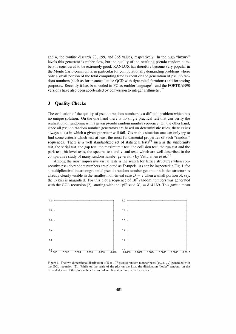
Among the most impressive visual tests is the search for lattice structures when con-secutive pseudo random numbers are plotted as D-tupels. As can be inspected in Fig. 1, fora multiplicative linear congruential pseudo random number generator a lattice structure isalready clearly visible in the smallest non-trivial case D = 2 when a small portion of, say,the x-axis is magnified. For this plot a sequence of 107 random numbers was generatedwith the GGL recursion (2), starting with the “pi”-seed X0 = 314 159. This gave a mean

0.000 0.002 0.004 0.006 0.008 0.0100.0

0.2

0.4

0.6

0.8

1.0

0.0000 0.0002 0.0004 0.0006 0.0008 0.00100.0

0.2

0.4

0.6

0.8

1.0

Figure 1. The two-dimensional distribution of 5 × 106 pseudo random number pairs (xi, xi+1) generated withthe GGL recursion (2). While on the scale of the plot on the l.h.s. the distribution “looks” random, on theexpanded scale of the plot on the r.h.s. an ordered line structure is clearly revealed.

451

value of x = 0.499 795 ≈ 1/2 and a variance of σ2 = x2 − x2 = 0.080 08 ≈ 1/12. Thefailure of the MLCG can easily be highlighted by intentionally using a “poor” choice ofparameters, for instance33 Xi+1 = (5Xi) mod 27, X0 = 1, where the problem becomesimmediately obvious.

When subjected to the various mathematical tests mentioned above, the R250 shiftregister generator turned out to be among the best generators. Consequently it has beenused in many Monte Carlo studies. It, therefore, came as a surprise when Ferrenberg et al.34

reported severe problems with this generator in applications to Monte Carlo simulations ofthe two-dimensional Ising model using the single-cluster Wolff update algorithm.35 Moreprecisely they performed simulations of a 16 × 16 square lattice with periodic boundaryconditions at the exactly known infinite-volume transition point βc = ln(1 +

√2)/2. They

generated 10 runs with 106 clusters each (which, on the average, cover at βc about 55%of the lattice sites). As a result Ferrenberg et al. obtained for the energy a systematicdeviation from the exact value36 of about 42σ (at an accuracy level of 0.003%) and forthe specific heat an even larger deviation of about −107σ (at an accuracy level of 0.03%).Further simulations with the same statistics but other pseudo random number generatorsbehaved perfectly well.

Subsequently these results have been confirmed by many other authors,37 and consen-sus has been reached that triplet correlations in 〈xnxn−kxn−250〉 around k = 147 are theorigin of the problem.38 Notice that due to “time-reversal symmetry” this value is equiv-alent39 to k = 250 − 147 = 103 – a value that just coincides with the second parameterq = 103 of the R250 generator! While the numerically determined correlator38 reproducesthe theoretically expected value of (1/2)3 = 0.125 for almost all values of k, it dropsdown to about 0.107 at k = 147 or equivalently39 at k = 103. This correlation doesnot only affect the cluster algorithm but also the Metropolis update which was shown38 tofail in combination with R250 at the tricritical point of the Blume-Capel model for some“resonant” lattice sizes.

By analyzing the recursion of R250 analytically, Heuer et al.39 succeeded to pre-dict an anomalous triplet correlation of 3/28 ≈ 0.107 142 857 1 . . . at the special valuek = 103, in perfect agreement with the numerical observation (which they also recon-firmed). Equipped with this finding they were able to propose a modified version of R250denoted as R250/521, which avoids these triplet correlations and indeed shows a muchimproved performance. For the two-dimensional Ising model on a 16 × 16 lattice at βc

they obtained with the R250/521 generator for the energy and specific heat systematic de-viations of absolutely tolerable (and in fact, expected) 0.1σ and 1.5σ, respectively, for aset-up of the single-cluster Monte Carlo simulations which was otherwise equivalent tothat of Ref. 34. This remarkable improvement indicates that the triplet correlations arevery probably responsible for the systematic errors observed by Ferrenberg et al.34

Around the same time, Shchur and Blote40 performed a systematic study of this prob-lem by varying the size L of the square lattice as well as the “magic numbers” (p, q),investigating the four pairs (p, q) = (36, 11), (89, 38), (127, 64), and (250, 103). For allpairs they found at βc significant deviations from the exact result with a maximum forL = 7, 12, 15, and 22, respectively. Since the average cluster size 〈C〉 of the single-clusterWolff update algorithm is an (improved) estimator41 for the susceptibility of Ising models,it scales with lattice size according to 〈C〉 = aLγ/ν , which in two dimensions specializesto 〈C〉 = aL7/4. The coefficient a is non-universal, and for the square geometry it takes the

452

generator periodic b.c. anti-periodic b.c.e c e c

R250 1.414 087(63) 1.356 9(16) 1.214 173(47) 0.704 52(85)−2.0σ +19.4σ −1.6σ +7.5σ

R250/521 1.414 206(59) 1.325 5(16) 1.214 277(47) 0.698 17(86)−0.14σ −0.27σ +0.6σ +0.06σ

RANLUX 1.414 253(60) 1.326 9(13) 1.214 215(48) 0.698 08(82)+0.65σ +0.75σ −0.7σ −0.05σ

exact/average 1.414 213 6 1.325 927 9 1.214 247(34) 0.698 08(82)

Table 1. Comparison of the energy e and specific heat c for a 10× 192 Ising system as obtained in single-clusterMonte Carlo simulations using three different pseudo random number generators. The deviations from the exact(periodic b.c.) respectively average (anti-periodic b.c.) values are given in units of the standard deviation σ,indicated in parentheses behind the mean values.

numerically determined value of a ≈ 1.1. Using this value in the above finite-size scalingformula one easily derives 〈C〉 ≈ 33, 85, 126, 141 = 0.55 × 256, and 246 for L = 7, 12,15, 16, and 22, respectively. By comparing with the parameter p one thus concludes thatthe largest deviations from the exact results happen when the average cluster size coincideswith p.

Also for asymmetric, strip-like lattices of size 10×192 the failure of the R250 generatorin combination with the single-cluster update algorithm was observed.42 Here periodicboundary conditions (b.c.) were applied in the long direction and both, periodic as wellas anti-periodic b.c., in the short direction. The results shown in Table 1 are based on2 × 106 measurements at βc. Here the deviations of the energy and specific heat from theexact results are less pronounced than in Refs. 34 and 40. This is, however, consistent withthe observation in Ref. 40, since the average cluster sizes, 〈C〉 ≈ 159 and 〈C〉 ≈ 83 forperiodic and anti-periodic b.c., respectively, are relatively far away from the lag p = 250.The modified generator R250/521 as well as RANLUX (in “luxury” level LUX = 4), on the

generator periodic b.c. anti-periodic b.c.ξe ξσ ξe ξσ

R250 1.5796(46) 12.7092(92) 0.7803(84) 4.2878(43)−0.3σ +3.3σ −3.8σ −0.7σ

R250/521 1.5851(48) 12.6787(74) 0.8110(82) 4.2925(39)+0.8σ −0.02σ −0.1σ +0.5σ

RANLUX 1.5770(50) 12.6789(85) 0.8126(83) 4.2887(40)−0.8σ +0.006σ +0.1σ −0.5σ

exact/average 1.5812(35) 12.678 845 0.8118(58) 4.2906(28)

Table 2. Same comparison as in Table 1 for the correlation lengths ξe and ξσ of energy and magnetizationdensities, respectively, in the long direction of a 10 × 192 Ising lattice.

453

other hand, performed very well. When using the R250 generator, small but still significantdeviations were also observed42 for the correlation lengths of the energy and spin densities(measured using the zero-momentum technique43), cf. Table 2.

Another simulational test based on Schwinger-Dyson identities has been proposed byBallesteros and Martın-Mayor.44 Applications to the two- and three-dimensional Isingmodel confirmed the flaws in two dimensions reported earlier and showed that also in threedimensions the combination of R250 with the single-cluster update algorithm producesincorrect results.

4 Non-Uniform Pseudo Random Numbers

All basic pseudo random number generators discussed above are designed for uniformlydistributed pseudo random numbers xi ∈ [0, 1). In many applications it is necessary,however, to be able to draw pseudo random numbers from non-uniform distributions.45

One strategy is to divide this problem into two parts. First, one of the generators describedabove is used to generate uniformly distributed random numbers, which in a second stepare appropriately transformed to follow the specific distribution at hand.

A standard procedure is the inversion method. For a given normalized probabilitydensity f(x) one calculates the associated probability distribution (accumulated density inusual physics terms),

F (x) =

∫ x

xmin

dx′f(x′) . (19)

Due to F ′(x) = f(x) ≥ 0 and the normalization condition, F (x) grows monotonicallyfrom 0 to 1, such that the F values are uniformly distributed. Drawing a uniformly dis-tributed pseudo random number R, equating R = F (x) and, if the function inverse isknown analytically, setting x = F−1(R) the problem is solved.

For the example of an exponential decay,

f(x) = exp(−x) , x ≥ 0 , (20)

one derives in this way R = F (x) = 1 − exp(−x) or

x = − ln(1 − R) , R ∈ [0, 1) . (21)

Notice that since R ∈ [0, 1), the formula should be programed in the “complicated” wayas shown here; rewriting it as x = − ln(R) one could occasionally hit ln 0 which wouldcause a run-time error (with a reaction depending on the operating system used).

Another simple example is the Lorentzian density

f(x) =1

π

Γ

Γ2 + x2, (22)

where Γ parameterizes the width of the Lorentzian peak. Here one calculatesR = F (x) = 1

π

∫ x

−∞dx′ Γ

Γ2+x′2 = 1

2+ 1

π tan−1( xΓ), which can be inverted to give

x = Γ tan [π(R − 1/2)] , R ∈ [0, 1) . (23)

454

The final and most important example are Gaussian random numbers which follow theprobability density (. . . no problem to remember if you saved a German 10 DM note . . . )

f(x) =1√

2πσ2exp

(

− x2

2σ2

)

, (24)

where the parameter σ2 is the squared width of the distribution. Here

R = F (x) =1√

2πσ2

∫ x

−∞

dx′ exp

(

− x′2

2σ2

)

=1

2

[

1 + erf

(

x√2σ2

)]

, (25)

with erf(·) denoting the error function which cannot be inverted analytically. Either onecould think of numerical inversion schemes (which indeed is the method of choice for re-ally complicated probability distributions) – or one remembers the polar coordinates trickused to calculate the Gaussian integral and continues analytically: Considering the auxil-iary two-dimensional product distribution f2(x, y) = f(x)f(y) = 1

2πσ2 exp(−x2+y2

2σ2 ) andintroducing polar coordinates x = r cos(Θ), y = r sin(Θ), one obtains

f2(x, y)dxdy =1

σ2exp(− r2

2σ2)rdr

dΘ

2π, (26)

showing immediately that the angle Θ is uniformly distributed between 0 and 2π. Also forthe radial coordinate r the inversion is now straightforward since

R1 = F (r) =1

σ2

∫ r

0

dr′r′ exp

(

− r′2

2σ2

)

= 1 − exp

(

− r2

2σ2

)

. (27)

We thus arrive at the so-called Box-Muller method: Draw two uniformly distributed ran-dom numbers R1 and R2, and compute

r =√

−2σ2 ln(1 − R1) , R1 ∈ [0, 1) , (28)Θ = 2πR2 , R2 ∈ [0, 1) . (29)

Then

x = r cos(Θ) , (30)y = r sin(Θ) , (31)

is a pair of two independent Gaussian distributed pseudo random numbers.Especially for Gaussian random numbers there is another procedure which directly

makes use of the central limit theorem and the fact that averages of arbitrarily distributedrandom numbers (under certain rather mild conditions) tend asymptotically to a Gaussiandistribution. In practice one uses, of course, again uniformly distributed pseudo randomnumbers xi generated with one of the algorithms described in the previous section. Re-calling the mean value x = 1/2 and variance σ2 = x2 − x2 = 1/12 for uniform randomnumbers, it is straightforward to see that

X =

(

n∑

i=1

xi −n

2

)

√

12

n(32)

is (approximately) a Gaussian distributed random number around X = 0 with unit vari-ance. Of course, since Xmax = −Xmin =

√3n, this can be strictly true only asymptot-

ically as n → ∞. But even the convenient choice n = 12 leads already to a reasonableapproximation46 in the range |X | < 2 = 2σ with errors less than 9 × 10−3.

455

Another, physically motivated direct method based on simulating N molecules hasrecently been discussed by Fernandez and Criado.47

5 Summary

The generation of “good” pseudo random numbers is quite a delicate issue that requiressome care and extensive quality tests. It is therefore highly recommended not to invent onesown “secret” recursion rules but to use one of the well-known generators which have beentested and applied by many other workers in the field. If such a well-accepted generatorwould turn out to be problematic in some specific application, one could at least be sure thatthe Monte Carlo community as a whole would work hard to track the origin of the problem– as it has happened with the (in)famous R250 generator. Being based on deterministicrecursion rules, it is trivial that for any pseudo random number generator one can design atest where it would fail. Thanks to the by now available quite sophisticated mathematicaland physically motivated empirical tests one can be very confident, however, that standardgenerators will yield sufficiently “random” numbers in most applications.

Acknowledgments

I would like to thank Tilman Sauer, Andreas Weber and Martin Weigel for pseudo random,but very useful discussions on randomly selected topics relevant for these lecture notes.

References

1. D. Frenkel and B. Smit, Understanding Molecular Simulation – From Algorithms toApplications (Academic Press, San Diego, 1996).

2. D.P. Landau and K. Binder, A Guide to Monte Carlo Simulations in Statistical Physics(Cambridge University Press, Cambridge, 2000).

3. F. Gutbrod, in: Annual Review of Computational Physics VI, ed. D. Stauffer (WorldScientific, Singapore, 1999), p. 203.

4. D. Stauffer, in: Computational Physics: Selected Methods – Simple Exercises – Se-rious Applications, eds. K.H. Hoffmann and M. Schreiber (Springer, Berlin, 1996),p. 1.

5. I. Vattulainen, K. Kankaala, J. Saarinen, and T. Ala-Nissila, Comp. Phys. Comm. 86,209 (1995).

6. I Vattulainen, Licentiate in Technology thesis, University of Helsinki (1994) [cond-mat/9411062].

7. K. Kankaala, T. Ala-Nissila, and I. Vattulainen, Phys. Rev. E48, R4211 (1993).8. I. Vattulainen, T. Ala-Nissila, and K. Kankaala, Phys. Rev. Lett. 73, 2513 (1994).9. I. Vattulainen, T. Ala-Nissila, and K. Kankaala, Phys. Rev. E52, 3205 (1995).

10. D.H. Lehmer, in: Proc. 2nd Symp. on Large-Scale Digital Calculating Machinery(Harvard University Press, Cambridge, 1951), p. 141.

11. S.K. Park and K.W. Miller, Comm. ACM 31, 1192 (1988).12. W.H. Press, S.A. Teukolsky, W.T. Vetterling, and B.P. Flannery, Numerical Recipes in

Fortran 77 – The Art of Scientific Computing, second corrected edition (CambridgeUniversity Press, Cambridge, 1996), pp. 269-270.

456

13. NAG Fortran Library Manual, Mark 14, 7 (Numerical Algorithms Group Inc., 1990).14. S.L. Anderson, SIAM Review 32, 221 (1990).15. G.S. Fishman, Math. Comp. 54, 331 (1990).16. A. De Matteis and S. Pagnutti, Parallel Computing 13, 193 (1990).17. G. Marsaglia, in: Applications of Number Theory to Numerical Analysis, ed. S.K.

Zaremba (Academic Press, New York, 1972), p. 249.18. W.H. Press, S.A. Teukolsky, W.T. Vetterling, and B.P. Flannery, in Ref. 12, p. 273.19. D.E. Knuth, The Art of Computer Programming, Volume 2: Seminumerical Algo-

rithms, second edition (Addison-Wesley, Reading, Massachusetts, 1981).20. T.G. Lewis and W.H. Payne, J. Assoc. Comput. Mach. 20, 456 (1973).21. R.C. Tausworthe, Math. Comp. 19, 201 (1965).22. S. Kirkpatrick and E.P. Stoll, J. Comp. Phys. 40, 517 (1981).23. G. Marsaglia and A. Zaman, Stat. & Prob. Lett. 8, 329 (1990).24. F. James, A Review of Pseudorandom Number Generators, Comp. Phys. Comm. 60,

329 (1990).25. G. Marsaglia, B. Narasimham, and A. Zaman, Comp. Phys. Comm. 60, 345 (1990).26. G. Marsaglia and A. Zaman, Ann. Appl. Prob. 1, 462 (1991).27. Private communication (1993) of F. James to M. Luscher (Ref. 28).28. M. Luscher, Comp. Phys. Comm. 79, 100 (1994).29. F. James, Comp. Phys. Comm. 79, 111 (1994).30. F. James, Comp. Phys. Comm. 97, 357 (1996).31. K.G. Hamilton, Comp. Phys. Comm. 101, 249 (1997).32. K.G. Hamilton and F. James, Comp. Phys. Comm. 101, 241 (1997).33. P. Blaudeck, in: Computational Physics: Selected Methods – Simple Exercises – Se-

rious Applications, eds. K.H. Hoffmann and M. Schreiber (Springer, Berlin, 1996),p. 9.

34. A.M. Ferrenberg, D. P. Landau, and Y.J. Wong, Phys. Rev. Lett. 69, 3382 (1992).35. U. Wolff, Phys. Rev. Lett. 62, 361 (1989); Nucl. Phys. B322, 759 (1989).36. B. Kaufman, Phys. Rev. 76, 1232 (1949); A.E. Ferdinand and M.E. Fisher, Phys.

Rev. 185, 832 (1969). For a Fortran code, see W. Janke, in: Computational Physics:Selected Methods – Simple Exercises – Serious Applications, eds. K.H. Hoffmann andM. Schreiber (Springer, Berlin, 1996), p. 10, and the accompanying diskette.

37. P.D. Coddington, Int. J. Mod. Phys. C5, 547 (1994) [cond-mat/9309017].38. F. Schmid and N.B. Wilding, Int. J. Mod. Phys. C6, 781 (1995) [cond-mat/9512135].39. A. Heuer, B. Dunweg, and A.M. Ferrenberg, Comp. Phys. Comm. 103, 1 (1997).40. L.N. Shchur and H.W.J. Blote, Phys. Rev. E55, R4905 (1997) [cond-mat/9703050].41. U. Wolff, Nucl. Phys. B334, 581 (1990).42. M. Weigel, Diploma thesis, Universitat Mainz (1998), unpublished.43. M. Weigel and W. Janke, Phys. Rev. Lett. 82, 2318 (1999); Phys. Rev. B62, 6343

(2000).44. H.G. Ballesteros and V. Martın-Mayor, Phys. Rev. E58, 6787 (1998).45. L. Devroye, Non-Uniform Random Variate Generation (Springer, Berlin, 1986).46. M. Abramowitz and I.A. Stegun (eds.), Handbook of Mathematical Functions, 9th

printing (Dover, New York, 1972), p. 953.47. J.F. Fernandez and C. Criado, preprint cond-mat/9901202.

457