PSF Estimation using Sharp Edge Prediction

Neel Joshi† Richard Szeliski∗ David J. Kriegman†

†University of California, San Diego ∗Microsoft Research

Abstract

Image blur is caused by a number of factors such as mo-tion, defocus, capturing light over the non-zero area of theaperture and pixel, the presence of anti-aliasing filters on acamera sensor, and limited sensor resolution. We present analgorithm that estimates non-parametric, spatially-varyingblur functions (i.e., point-spread functions or PSFs) at sub-pixel resolution from a single image. Our method handlesblur due to defocus, slight camera motion, and inherent as-pects of the imaging system. Our algorithm can be used tomeasure blur due to limited sensor resolution by estimatinga sub-pixel, super-resolved PSF even for in-focus images.It operates by predicting a “sharp” version of a blurry in-put image and uses the two images to solve for a PSF. Wehandle the cases where the scene content is unknown andalso where a known printed calibration target is placed inthe scene. Our method is completely automatic, fast, andproduces accurate results.

1. Introduction

Image blur is introduced in a number of stages in a cam-era. The most common sources of image blur are motion,defocus, and aspects inherent to the camera, such as pixelsize, sensor resolution, and the presence of anti-aliasing fil-ters on the sensor.

When blur is undesirable, one can deblur an image usinga deconvolution method, which requires accurate knowl-edge of the blur kernel. In applications where blur is de-sirable and essential, such as shape from defocus, it is stillnecessary to recover the shape and size of the spatially vary-ing blur kernel.

Recovering a PSF from a single blurred image is an in-herently ill-posed problem due to the loss of informationduring blurring. The observed blurred image provides onlya partial constraint on the solution, as there are many com-binations of PSFs and “sharp” images that can be convolvedto match the observed blurred image.

Prior knowledge about the image or kernel can disam-biguate the potential solutions. Early work in this area sig-nificantly constrained the form of the kernel [6], while morerecently, researchers have put constraints on the underlyingsharp image [3]. In our work, we take the latter approach;however, instead of using statistical priors, we leverage ourprior assumption more directly. Specifically, we present analgorithm for estimating regions of a sharp image from ablurry input—if one can estimate the sharp image, recover-

Min

Max

R R

Valid Region

Figure 1. Sharp Edge Prediction. A blurry image (top left) and the1D profile normal to an edge (top right, blue line). We predict asharp edge (top right, dashed line) by propagating the max and minvalues along the edge profile. The algorithm uses predicted andobserved values to solve for a PSF. Only observed pixels within aradius R are used. (bottom left) Predicted pixels are blue and validobserved pixels are green. (bottom right) The predicted values.

ing the blur kernel is possible.The key insight of our work is that with certain types of

image blur, the location of image features such as edges aredetectable even if the feature strength is weakened. Whenthe scene content is unknown, we detect edges and predictthe underlying sharp edges that created the blurred obser-vations, under the assumption that detected edge was a stepedge before blurring. Each pair of predicted and blurrededges gives information about a radial profile of the PSF.If an image has edges spanning all orientations, the blurredand predicted sharp image contain enough information tosolve for a general two-dimensional PSF.

For situations where the scene content can be controlled,we have designed a printed calibration target whose imageis automatically aligned with a known representation of thetarget. We then use this pair to solve for an accurate PSF.

Our method has several advantages over previous ap-proaches: it measures the entire PSF of an image systemfrom world to image, it is fast and accurate, and it can solvefor spatially varying PSFs at sub-pixel resolution using onlya single image.

We show results for both unknown scenes and imagesof our calibration target. We present deconvolution resultsusing the recovered PSFs to validate the blur kernels andshow a synthetic experiment to further evaluate the method.

Motion BlurRadial

DistortionDefocus Blur

Anti-Aliasing

Perspective Transform

Sensor Sampling

Geometric Transformations Point Spread Function

Figure 2. Image Formation Model. The imaging model consists of two geometric transforms as well as blur induced by motion, defocus,sensor anti-aliasing, and finite-area sensor sampling. We solve for an estimate of the continuous point-spread function at each discretelysampled (potentially blurry and noisy) pixel.

We also show that by solving for spatially varying, per-colorchannel PSFs combined with per-channel radial distortioncorrections, we can remove chromatic aberrations artifacts.

2. Related Work

The problem of blur kernel estimation and more gener-ally blind deconvolution is a longstanding problem in com-puter vision and image processing. The entire body of pre-vious work in this area is beyond what can be covered here.For a more in depth study of much of the earlier work inblur estimation, we refer the reader to the survey paper byKundur and Hatzinakos [6].

In the computer vision literature, classical shape-from-defocus [10] addresses PSF estimation using a parametricmodel for blur that is either a “pillbox” or 2D Gaussianfunction with a single parameter for the PSF size, i.e., fo-cal length or kernel radius. For more complex blurs, suchas motion blur, many recent single-image estimation tech-niques model blurs as a collections of 1D or 2D box blursand use segmentation techniques to handle multiple mo-tions [7, 4, 2]. Shan et al. [12], on the other hand, use alow-parameter model to remove motion blur due to an ob-ject translating and rigidly rotating about an axis parallelto the camera’s optical axis. In contrast with this previouswork, we do not use a parametric model for the PSF andsolve for spatially varying kernels without performing anyexplicit segmentation.

There is significantly less work in the area of single im-age blur estimation using non-parametric kernels. The workby Fergus et al. [3] is perhaps the most notable method ofthis type. Fergus et al. use natural image statistics to derivean image prior that is used in a variational Bayes formula-tion. In contrast, we leverage prior assumptions on imagesto directly predict the underlying sharp image. We considerour approach complementary to that of Fergus et al., as ourmethod excels at accurately computing smaller kernels, andit can be used for lens and sensor characterization. Theirmethod is not as well suited to these applications, but excelsat computing large kernels due to complex camera motion,which is outside the scope of our work.

Our work is conceptually most similar to slant-edge cal-ibration [11, 1]. These methods recover 1D blur profiles byimaging a slanted edge feature and finding the 1D kernel

normal to the edge profile that gives rise to the blurred ob-servations of the known step edge. Reichenbach et al. [11]note that one can combine several 1D sections to estimatea 2D PSF. We take a similar approach philosophically toslant-edge techniques, with three major differences: we ex-tend the method to directly solve for 2D PSFs, we solvefor spatially varying PSFs, and we present a blind approachwhere the underlying step edge is not know a priori.

A related area is modulation transfer function (MTF)estimation for lenses that uses images of random dot pat-terns [8]. In theory, infinitesimal dot patterns are useful forPSF estimation, but in practice, it is not possible to createsuch a pattern. In contrast, creating sharp step edges is rela-tively easy and thus generally preferable [11]. An additionaladvantage of our work relative to using dot patterns is thatby using a grid-like structure with regular, detectable cor-ner features, we can compute a radial distortion correctionin addition to estimating PSFs.

3. Image Formation Model

We now give a brief overview of relevant imaging andoptics concepts needed for PSF estimation. As illustratedin Figure 2, the imaging model consists of two geomet-ric transforms: a perspective transform (used when pho-tographing a known planar calibration target) and a radialdistortion. There are several sources of blur induced by mo-tion, defocus, sensor anti-aliasing, and pixel sampling area(fill factor and active sensing area shape). We model allblur as a convolution along the image plane and account fordepth dependent defocus blur and 3D motion blur by allow-ing for the PSF to be spatially varying.

Our method estimates a discretely sampled version ofthe continuous PSF by either matching the sampling to theimage resolution (which is useful for estimating large blurkernels) or using a sub-pixel sampling grid to estimate adetailed PSF, which captures effects such as anti-aliasingof the sensor and allows us to do more accurate imagerestoration. In addition, by computing a sub-pixel PSF, wecan perform single-image super-resolution by deconvolvingup-sampled images with the recovered PSF.

Geometric Transformations: The world to imagetransformation consists of a perspective transform and a

radial distortion. With the blind method, we ignore theperspective transform and operate in image coordinates.

With the non-blind method, where we photograph aknown calibration target, we model the perspective trans-formation as a 2D homography to map known feature loca-tions F k on the grid pattern to detected feature points fromthe image F d. We use a standard model for radial distor-tion: (F ′

x, F ′y)T = (Fx, Fy)T (a0+a1r

2(x, y)+a2r4(x, y)),

where r(x, y) =√

F 2x + F 2

y is the radius relative to the im-age center.

Given a radial distortion function R(F ) and warpfunction which applies a homography H(F ), the fullalignment process is F d = R(H(F k)). We compute theparameters that minimize the L2 norm of the residual||F d − R(H(F k))||2. Computing these parameters cannotbe done simultaneously in closed form. However, theproblem is bilinear, and thus we solve for the parametersusing an iterative approach.

Modeling the Discrete Point-Spread Function: Theequation for the observed image B is a convolution of akernel K and a potentially higher resolution sharp imageI , plus additive Gaussian white noise, whose result ispotentially down-sampled:

B = D(I ⊗K) + N, (1)where N ∼ N (0, σ2). D(I) down-samples an image bypoint-sampling IL(m, n) = I(sm, sn) at a sampling rate sfor integer pixel coordinates (m, n). In our formulation, thekernel K models all blurring effects, which are potentiallyspatially varying and wavelength dependent.

4. Sharp Image Estimation

The blurring process is formulated as an invertible linearsystem, which models the blurry image as the convolutionof a sharp image with the imaging system’s PSF. Thus, ifwe know the original sharp image, recovering the kernel isstraightforward. The key contribution of our work is a re-liable and widely applicable method for predicting a sharpimage from a single blurry image. In the following sec-tion, we present our methods for predicting the sharp im-age. In Section 5, we discuss how to formulate and solvethe invertible linear system to recover the PSF. In the fol-lowing discussion, we consider images to be single channelor grayscale; in Section 6, we discuss color images.

4.1. Blind Estimation

For blind sharp image prediction, we assume blur is dueto a PSF with a single mode (or peak), such that when animage is blurred, the ability to localize a previously sharpedge is unchanged; however, the strength and profile of theedge is changed, as illustrated in Figure 1. Thus, by localiz-ing blurred edges and predicting sharp edge profiles, locallyestimating a sharp image is possible.

We assume that all observed blurred edges result fromconvolving an ideal step edge with the unknown kernel.Our algorithm finds the location and orientation of edgesin the blurred image using a sub-pixel difference of Gaus-sians edge detector. It then predicts an ideal sharp edge byfinding the local maximum and minimum pixel values, ina robust way, along the edge profile and propagates thesevalues from pixels on each side of an edge to the sub-pixeledge location. The pixel on the edge itself is colored accord-ing to the weighted average of the maximum and minimumvalues according to the distance of the sub-pixel location tothe pixel center, which is a simple form of anti-aliasing (seeFigure 1).

To find the maximum value, our algorithm marchesalong the edge normal, sampling the image looking for a lo-cal maximum using hysteresis. Specifically, the maximumlocation is the first pixel that is less than 90% (as opposed tostrictly less than) of the previous value. Once this value andlocation are identified, we store the “maximum” value asthe mean of all values along the edge profile that are within10% of the initial maximum value. An analogous approachis used for the minimum.

Since we can only reliably predict values near edges, weonly use observed pixels within a radius of the predictedsharp values. These locations are stored as valid pixels in amask, which is used when solving for the PSF, as discussedin Section 5. At the end of the prediction process, we havea partially estimated sharp image, as shown in Figure 1.

4.2. Non-Blind Estimation

For non-blind sharp edge prediction, we want to com-pute the PSF given that we know the sharp image. Sincewe anticipate using this technique in a controlled lab setup,we designed a special calibration pattern for this purpose(Figure 3). We take an image of this pattern and alignthe known grid pattern to the image to get the sharp/blurrypair needed to compute the PSF accurately. The grid hascorner (checkerboard) features so that it can be automati-cally detected and aligned, and it also has sharp step edgesequally distributed at all orientations within a tiled pattern,so that it provides edges that capture every radial slice ofthe PSF. (Alternatively, we can say that the calibration pat-terns provides measurable frequencies at all orientations.)Furthermore, we represent the grid in mathematical form(the curved segments are 90◦ arcs), which gives us a veryprecise definition for the grid, which is advantageous forperforming alignment.

For non-blind prediction, we continue to assume that ker-nel has no more than a single peak. Thus even when thepattern is blurred, we can detect corners on the grid with asub-pixel corner detector. Because our corners are actuallybalanced checkerboard crossings (radially symmetric), theydo not suffer from “shrinkage” (displacement) due to blur-

Figure 3. Non-Blind Estimation. (left) The tiled calibration pat-tern, (middle) cropped section of an image of a printed version ofthe grid, and (right) the corresponding cropped part of the knowngrid warped and shaded to match the image of the grid.

ring. Once corners are found, the ground truth pattern isaligned to the acquired image. To obtain an accurate align-ment, we correct for both geometric and radiometric aspectsof the imaging system.

We perform geometric alignment using the correctionsdiscussed in Section 3. We fit a homography and radial dis-tortion correction to match the known feature locations onthe grid pattern to corners detected with sub-pixel precisionon the acquired (blurry) image of the printed grid.

We also must account for the lighting and shading in theimage of the grid. We do this by first aligning the knowngrid to the image. Then, for each edge location (as knownfrom mathematical form of the ground truth grid pattern),the algorithm finds the maximum and minimum values onthe edge profile and propagates them just as in the non-blindapproach. We shade the grid for pixels within the blur ra-dius of each edge. By performing the shading operation,our algorithm has corrected for shading, lighting, and radialintensity falloff. Figure 3 shows the results of the geometricwarp and shading transfer.

5. PSF Estimation

Once the sharp image is predicted, we estimate the PSFas the kernel that, when convolved with the sharp image,produces the blurred input image. We formulate the estima-tion using a Bayesian framework solved using a maximum aposteriori (MAP) technique. In MAP estimation, one triesto find the most likely estimate for the blur kernel K giventhe sharp image I and the observed blurred image B, usingthe known image formation model and noise level.

We express this as a maximization over the probabilitydistribution of the posterior using Bayes’ rule. The result isminimization of a sum of negative log likelihoods L(.):

P (K|B) = P (B|K)P (K)/P (B) (2)argmax

KP (K|B) = argmin

KL(B|K) + L(K). (3)

The problem is now reduced to defining the negative loglikelihood terms. Given the image formation model (Equa-tion 1), the data term is:

L(B|K) = ||M(B)−M(I ⊗K)||2/σ2. (4)

(The downsampling term D in (1) will be incorporated inSection 5.1.) M(.) is a masking function such that this term

is only evaluated for “known” pixels in B, i.e., those pixelsthat result from the convolution of K with properly esti-mated pixels I , which form a band around each edge point,as described in Section 4.1.

The remaining negative log likelihood term, L(K), mod-els prior assumptions on the blur kernel and regularizes thesolution. We use a smoothness prior and a non-negativityconstraint. The smoothness prior penalizes large gradientsand thus biases kernel values to take on values similar totheir neighbors: Ls(K) = λγ||∇K||2. λ controls theweight of the smoothness penalty, and γ = (2R + 1)2 nor-malizes for the kernel area (R is the kernel radius). Sincethe kernel should sum to one (as blur kernels are energyconserving) the individual values decrease with increasedR. This factor is needed to keep the relative magnitude ofkernel gradient values on par with the data term values re-gardless of kernel size.

We minimizing the following error function:

L = ||M(B)−M(I ⊗K)||2/σ2 + λγ||∇K||2, (5)

subject to Ki ≥ 0, to solve for the PSF using non-negativelinear least squares using a projective gradient Newton’smethod. We currently estimate the noise level σ using atechnique similar to that of Liu et al. [9], and we have em-pirically found λ = 2 to work well.

5.1. Computing a Super-Resolved PSF

By taking advantage of sub-pixel edge detection forblind prediction and sub-pixel corner detection for non-blind prediction, we can estimate a super-resolved blur ker-nel by predicting a sharp image at a higher resolution thanthe observed image.

For the blind method, in the process of estimating thesharp image, it is necessary to rasterize the predicted sharpedge-profile back onto a pixel grid. By rasterizing the sub-pixel sharp-edge profile onto an up-sampled grid, we can es-timate a super-resolved sharp image. In addition, at the ac-tual identified edge location (as before), the pixel color is aweighted average of the minimum and maximum, where theweighting reflects the sub-pixel edge location on the grid.

For the non-blind method, we also must rasterize thegrid pattern at a some desired resolution. Since we detectcorners at sub-pixel precision, the geometric alignment iscomputed with sub-pixel precision. Using the mathemati-cal description of our grid, we can choose any upsampledresolution when rasterizing the predicted sharp image. Wealso perform anti-aliasing, as described in Section 4.2.

To solve for the PSF using the super-resolved predictedsharp image IH and the observed (vectorized) blurry im-age b, we modify Equation 4 to include a down-samplingfunction according to our image model (Equation 1). Weconsider b̂H = AHkH to be super-resolved sharp imageblurred by the super-resolved kernel kH , where AH is thematrix form of IH . Equation 4 is then ||b−DAHkH ||2 (we

0 degrees 45 degrees 90 degrees

13

Ground Truth Kernel Our Estimated Kernel Fergus et al. Kernel Ground Truth Kernel Our Estimated Kernel Fergus et al. Kernel Ground Truth Kernel Our Estimated Kernel Fergus et al. Kernel

Pixels

17

Ground Truth Kernel Our Estimated Kernel Fergus et al. Kernel Ground Truth Kernel Our Estimated Kernel Fergus et al. Kernel Ground Truth Kernel Our Estimated Kernel Fergus et al. Kernel

17Pixels

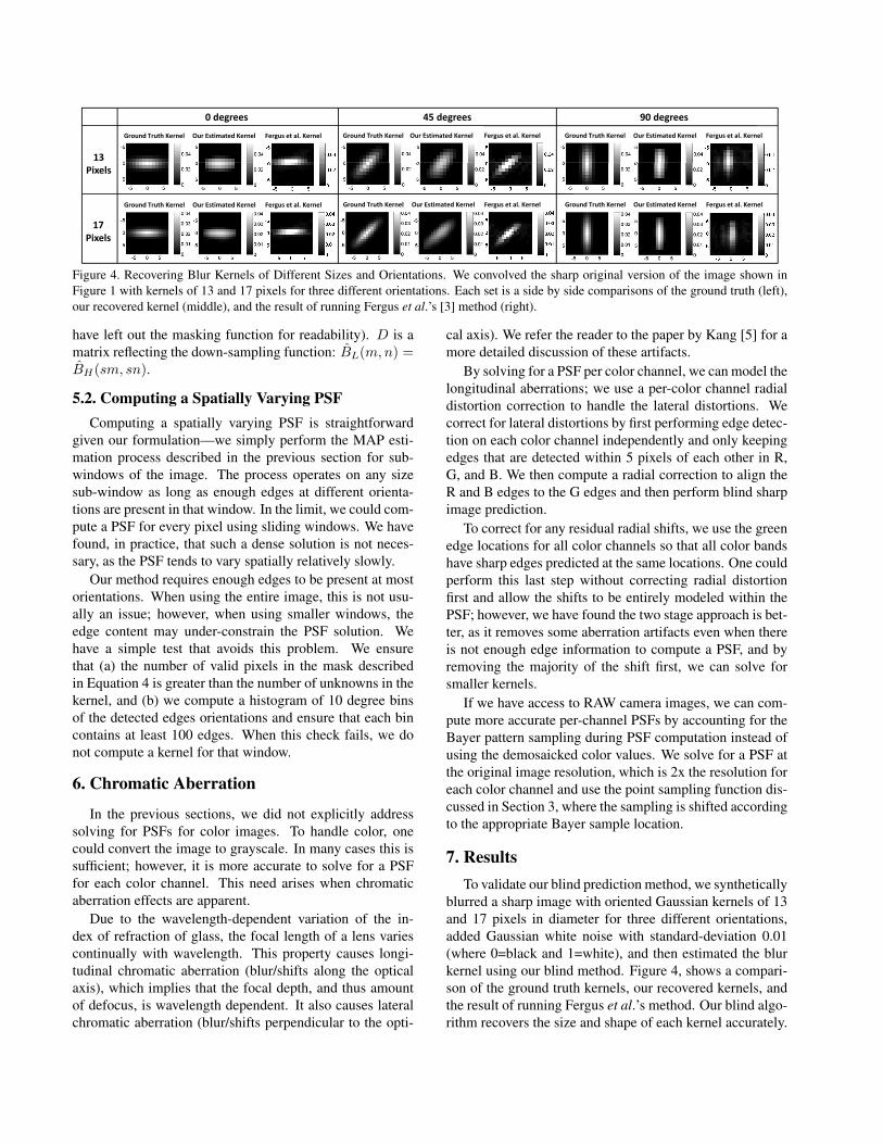
Figure 4. Recovering Blur Kernels of Different Sizes and Orientations. We convolved the sharp original version of the image shown inFigure 1 with kernels of 13 and 17 pixels for three different orientations. Each set is a side by side comparisons of the ground truth (left),our recovered kernel (middle), and the result of running Fergus et al.’s [3] method (right).

have left out the masking function for readability). D is amatrix reflecting the down-sampling function: B̂L(m, n) =B̂H(sm, sn).

5.2. Computing a Spatially Varying PSF

Computing a spatially varying PSF is straightforwardgiven our formulation—we simply perform the MAP esti-mation process described in the previous section for sub-windows of the image. The process operates on any sizesub-window as long as enough edges at different orienta-tions are present in that window. In the limit, we could com-pute a PSF for every pixel using sliding windows. We havefound, in practice, that such a dense solution is not neces-sary, as the PSF tends to vary spatially relatively slowly.

Our method requires enough edges to be present at mostorientations. When using the entire image, this is not usu-ally an issue; however, when using smaller windows, theedge content may under-constrain the PSF solution. Wehave a simple test that avoids this problem. We ensurethat (a) the number of valid pixels in the mask describedin Equation 4 is greater than the number of unknowns in thekernel, and (b) we compute a histogram of 10 degree binsof the detected edges orientations and ensure that each bincontains at least 100 edges. When this check fails, we donot compute a kernel for that window.

6. Chromatic Aberration

In the previous sections, we did not explicitly addresssolving for PSFs for color images. To handle color, onecould convert the image to grayscale. In many cases this issufficient; however, it is more accurate to solve for a PSFfor each color channel. This need arises when chromaticaberration effects are apparent.

Due to the wavelength-dependent variation of the in-dex of refraction of glass, the focal length of a lens variescontinually with wavelength. This property causes longi-tudinal chromatic aberration (blur/shifts along the opticalaxis), which implies that the focal depth, and thus amountof defocus, is wavelength dependent. It also causes lateralchromatic aberration (blur/shifts perpendicular to the opti-

cal axis). We refer the reader to the paper by Kang [5] for amore detailed discussion of these artifacts.

By solving for a PSF per color channel, we can model thelongitudinal aberrations; we use a per-color channel radialdistortion correction to handle the lateral distortions. Wecorrect for lateral distortions by first performing edge detec-tion on each color channel independently and only keepingedges that are detected within 5 pixels of each other in R,G, and B. We then compute a radial correction to align theR and B edges to the G edges and then perform blind sharpimage prediction.

To correct for any residual radial shifts, we use the greenedge locations for all color channels so that all color bandshave sharp edges predicted at the same locations. One couldperform this last step without correcting radial distortionfirst and allow the shifts to be entirely modeled within thePSF; however, we have found the two stage approach is bet-ter, as it removes some aberration artifacts even when thereis not enough edge information to compute a PSF, and byremoving the majority of the shift first, we can solve forsmaller kernels.

If we have access to RAW camera images, we can com-pute more accurate per-channel PSFs by accounting for theBayer pattern sampling during PSF computation instead ofusing the demosaicked color values. We solve for a PSF atthe original image resolution, which is 2x the resolution foreach color channel and use the point sampling function dis-cussed in Section 3, where the sampling is shifted accordingto the appropriate Bayer sample location.

7. Results

To validate our blind prediction method, we syntheticallyblurred a sharp image with oriented Gaussian kernels of 13and 17 pixels in diameter for three different orientations,added Gaussian white noise with standard-deviation 0.01(where 0=black and 1=white), and then estimated the blurkernel using our blind method. Figure 4, shows a compari-son of the ground truth kernels, our recovered kernels, andthe result of running Fergus et al.’s method. Our blind algo-rithm recovers the size and shape of each kernel accurately.

(a) (b) (c) (d) (e) (f)

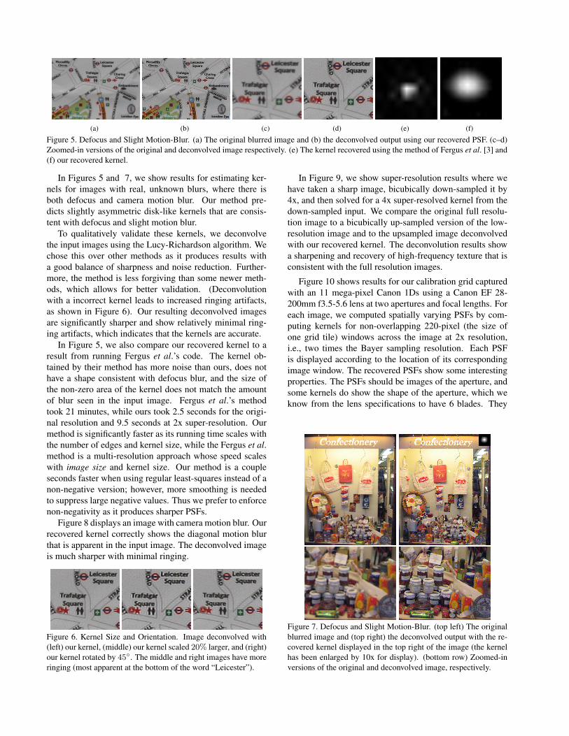
Figure 5. Defocus and Slight Motion-Blur. (a) The original blurred image and (b) the deconvolved output using our recovered PSF. (c–d)Zoomed-in versions of the original and deconvolved image respectively. (e) The kernel recovered using the method of Fergus et al. [3] and(f) our recovered kernel.

In Figures 5 and 7, we show results for estimating ker-nels for images with real, unknown blurs, where there isboth defocus and camera motion blur. Our method pre-dicts slightly asymmetric disk-like kernels that are consis-tent with defocus and slight motion blur.

To qualitatively validate these kernels, we deconvolvethe input images using the Lucy-Richardson algorithm. Wechose this over other methods as it produces results witha good balance of sharpness and noise reduction. Further-more, the method is less forgiving than some newer meth-ods, which allows for better validation. (Deconvolutionwith a incorrect kernel leads to increased ringing artifacts,as shown in Figure 6). Our resulting deconvolved imagesare significantly sharper and show relatively minimal ring-ing artifacts, which indicates that the kernels are accurate.

In Figure 5, we also compare our recovered kernel to aresult from running Fergus et al.’s code. The kernel ob-tained by their method has more noise than ours, does nothave a shape consistent with defocus blur, and the size ofthe non-zero area of the kernel does not match the amountof blur seen in the input image. Fergus et al.’s methodtook 21 minutes, while ours took 2.5 seconds for the origi-nal resolution and 9.5 seconds at 2x super-resolution. Ourmethod is significantly faster as its running time scales withthe number of edges and kernel size, while the Fergus et al.method is a multi-resolution approach whose speed scaleswith image size and kernel size. Our method is a coupleseconds faster when using regular least-squares instead of anon-negative version; however, more smoothing is neededto suppress large negative values. Thus we prefer to enforcenon-negativity as it produces sharper PSFs.

Figure 8 displays an image with camera motion blur. Ourrecovered kernel correctly shows the diagonal motion blurthat is apparent in the input image. The deconvolved imageis much sharper with minimal ringing.

Figure 6. Kernel Size and Orientation. Image deconvolved with(left) our kernel, (middle) our kernel scaled 20% larger, and (right)our kernel rotated by 45◦. The middle and right images have moreringing (most apparent at the bottom of the word “Leicester”).

In Figure 9, we show super-resolution results where wehave taken a sharp image, bicubically down-sampled it by4x, and then solved for a 4x super-resolved kernel from thedown-sampled input. We compare the original full resolu-tion image to a bicubically up-sampled version of the low-resolution image and to the upsampled image deconvolvedwith our recovered kernel. The deconvolution results showa sharpening and recovery of high-frequency texture that isconsistent with the full resolution images.

Figure 10 shows results for our calibration grid capturedwith an 11 mega-pixel Canon 1Ds using a Canon EF 28-200mm f3.5-5.6 lens at two apertures and focal lengths. Foreach image, we computed spatially varying PSFs by com-puting kernels for non-overlapping 220-pixel (the size ofone grid tile) windows across the image at 2x resolution,i.e., two times the Bayer sampling resolution. Each PSFis displayed according to the location of its correspondingimage window. The recovered PSFs show some interestingproperties. The PSFs should be images of the aperture, andsome kernels do show the shape of the aperture, which weknow from the lens specifications to have 6 blades. They

Figure 7. Defocus and Slight Motion-Blur. (top left) The originalblurred image and (top right) the deconvolved output with the re-covered kernel displayed in the top right of the image (the kernelhas been enlarged by 10x for display). (bottom row) Zoomed-inversions of the original and deconvolved image, respectively.

Figure 8. Motion Blur. (top row) The original blurred image (left)and the deconvolved output (right) with the recovered kernel dis-played in the top right of the image (the kernel has been enlargedby 10x for display). (bottom row) Zoomed-in versions of the orig-inal and deconvolved image, respectively.

also show “donut” artifacts that can occur at some settingswith lower-quality lenses. Perspective distortion across theimage plane and vignetting (clipping of the aperture) bythe lens barrel are also visible. For comparison we imagedback-lit pinholes at the same camera settings. Imaging pin-holes to measure PSFs has some inherent problems due tothe pinhole actually being a disk and not an infinitesimalpoint and due to diffraction; however, these images validateour recovered PSFs.

We also acquired a very sharply focused image, so thatwe could measure sub-pixel blur. Figure 11 shows an imageof our grid from a 6 mega-pixel Canon 1D, using a high-quality Canon EF 135mm f/2L lens. We show recoveredPSFs at 1x, 2x, 8x, and 16x sub-pixel sampling. The PSFsusing higher sub-pixel resolution show an interesting struc-ture that results from a combination of diffraction, lens im-perfections, and sensor anti-aliasing and sampling.

Figure 12 shows a result for performing blind chromatic

Figure 9. 4x Super-Resolution. (left) The original image andzoom-in, (middle) the original image bi-cubically downsampledand re-upsampled by 4x and zoom-in, (right) the upsampled imagedeconvolved using the recovered 4x super-resolved kernel (dis-played in the top right of the image–the kernel has been enlargedby 10x for display) and a zoom-in on the bottom.

(a) 150mm f5.6 (b) 145mm f10

Figure 10. Different Apertures and Focal Lengths. (first row)Cropped portions of the observed blurred images, (second row)recovered spatially varying PSFs (green channel only), (third row)images of pinholes at the same depths and settings, and (fourthrow) our recovered PSFs convolved with a disk the size of the pin-hole. For (a) each PSF is 33 × 33 pixels and (b) they are 41 × 41pixels. The PSFs reflect the shape of the aperture and show per-spective distortion and vignetting across the image plane.

aberration correction for a JPEG image from a Canon S60using a 5.8mm focal length at f8. After performing radialdistortion correction and piecewise deconvolution using thespatially varying PSF, the aberration artifacts are signifi-cantly reduced. Figure 13 shows chromatic aberration cor-rection for our non-blind method.

To view full resolution versions of our results, includingadditional examples, visit http://vision.ucsd.edu/kriegman-grp/research/psf estimation/.

8. Discussion and Future Work

We have shown how to recover spatially varying PSFs atsub-pixel precision that capture blur due to motion, defo-cus, and intrinsic camera properties. Our method is fast,straightforward to implement, and predicts kernels accu-rately for a wide variety of images. Nevertheless, ourmethod does have some limitations, and there are severalavenues for future work.

The primary limitation of our method is that we can onlysolve for kernels with a single peak. This limitation is dueto our reliance on an edge detector to find a single locationfor every blurred edge. In the case of a multi-peaked ker-nel, our method will incorrectly interpret the “ghost” copies

(a) (b) (c) (d) (e)

Figure 12. Blind Chromatic Aberration. (a) Recovered spatially varying PSFs for red, green, and blue shown as a color image. PSFs areonly computed where there are enough edges observed. (b) The original image, (c) after radial correction and deconvolution the aberrationsare significantly reduced, and (d–e) zoomed-in versions and intensity profiles for (b–c).

of edges as independent edges. While we have shownthat single-peaked kernels model many commonly occur-ring cases of blur, we would like to extend our method tohandle multi-modal kernels. One option is to group eachstronger edge with its weaker ghost edges using contourmatching. Once the ghost edges are identified, we couldperform sharp edge prediction only for the primary edges.

As each sharp edge profile gives information about a ra-dial slice of the PSF, it is necessary for an image, or imagewindow, to have edges (or at least high-frequency content)at most orientations. If some orientations are lacking, ourregularization terms can compensate; however, there is abreaking point, and there may not always be enough edgeinformation to properly compute a PSF. In these cases, alow parameter kernel model may be more appropriate, butour sharp image prediction could still be be used to improvemore traditional parametric kernel estimation procedures.We also plan to try using robust least squares to compensatefor erroneous edge detections or profile fits.

Lastly, we would like to characterize more lenses andcameras. We would like to build a database that the visionand photography community could contribute to by usingour pattern and code to take their own measurements.

9. Acknowledgements

We would like to thank the anonymous reviewers fortheir comments. This work was partially completed whilethe first author was an intern at Microsoft Research.

References

[1] P. D. Burns and D. Williams. Using slanted edge analysis forcolor registration measurement. In IS&T PICS Conference,

(a)

−2 −1 0 1 2

−2

−1

0

1

2

(b)

−2 −1 0 1 2

−2

−1

0

1

2

(c)

−2 −1 0 1 2

−2

−1

0

1

2

(d)

−2 −1 0 1 2

−2

−1

0

1

2

(e)

Figure 11. Sub-Pixel PSFs. (a) Cropped section of a sharp imageof our grid, (b) PSF (green channel only) at the Bayer resolution(1x), (b) 2x, (c), 8x, and (d) 16x sub-pixel sampling. The sub-pixelPSFs show blur resulting from a combination of diffraction, lensimperfections, and sensor anti-aliasing and sampling.

pages 51–53. Society for Imaging Science and Technology,1999.

[2] S. Cho, Y. Matsushita, and S. Lee. Removing non-uniformmotion blur from images. In ICCV 2007, pages 1–8, 14-21Oct. 2007.

[3] R. Fegus et al. Removing camera shake from a single pho-tograph. ACM Transactions on Graphics, 27(3):787–794,August 2006.

[4] J. Jia. Single image motion deblurring using transparency.In CVPR ’07, pages 1–8, 17-22 June 2007.

[5] S. B. Kang. Automatic removal of chromatic aberration froma single image. In CVPR ’07, pages 1–8, 17-22 June 2007.

[6] D. Kundur and D. Hatzinakos. Blind image deconvolution.SPMag, 13(3):43–64, May 1996.

[7] A. Levin. Blind motion deblurring using image statistics. InAdvances in Neural Information Processing Systems. MITPress, 2006.

[8] E. Levy, D. Peles, M. Opher-Lipson, and S. Lipson. Mod-ulation transfer function of a lens measured with a randomtarget method. Applied Optics, 38:679–683, Feb. 1999.

[9] C. Liu, W. T. Freeman, R. Szeliski, and S. B. Kang. Noiseestimation from a single image. In CVPR ’06, volume 2,pages 901–908, New York, NY, June 2006.

[10] S. Nayar, M. Watanabe, and M. Noguchi. Real-time focusrange sensor. In Fifth International Conference on Com-puter Vision (ICCV’95), pages 995–1001, Cambridge, Mas-sachusetts, June 1995.

[11] S. E. Reichenbach, S. K. Park, and R. Narayanswamy. Char-acterizing digital image acquisition devices. Optical Engi-neering, 30(2):170–177, February 1991.

[12] Q. Shan, W. Xiong, and J. Jia. Rotational motion deblurringof a rigid object from a single image. In ICCV 2007, pages1–8, 14-21 Oct. 2007.

Figure 13. Chromatic Aberration. (left) The recovered spatiallyvarying PSFs for red, green, and blue shown as a color image.The red and blue fringing is reflected in the PSF image and thePSFs are larger towards the edge of the image and spread alongthe direction orthogonal to the optical axis. (middle) Zoom-in onthe input image. (right) After radial correction and deconvolutionthe aberrations are significantly reduced.