PSTricks

1

pst-electricfieldElectric field lines of charges; v.0.13

July 2, 2010

Package author(s):Juergen GilgManuel LuquePatrice MegretHerbert Voß

1 Method based on electric flux (Patrice Mégret) 2

1 Method based on electric flux (Patrice Mégret)

Equipotential surfaces and E-field lines can be drawn by using the package pst-funcand the command \psplotImp[options](x1,y1)(x2,y2).

The following explanations describe the theory on which this is based.Gauss theorem states that the electric flux across a closed surface S and defined by:

ψ =

‹

S

~D · ~undS = Q (1)

is equal to the real charge Q inside S. As a consequence, in place where there is nocharge (Q = 0), the electric flux is a conservative quantity.

A tube of flux is a tube constructed on D-field lines and without charge, the flux goinginside any cross-section of the tube is equal to the flux going outside any cross-sectionof the tube. This means that, by following a tube of a given flux, we automatically followa D-field line. By using this technique, it is thus possible to obtain a scalar equation thatdescribes the D-field lines. This equation is an implicit equation and can be derived forsystems with simple geometrical properties.

Here the analysis will be limited to point charges and the D-field lines will thus beidentical to the E-field lines as there is no electric polarization.

For a point charge q, located at the origin of the coordinate system, the electric fieldand the potential are given by:

~E =1

4πε0εrq~r

|~r|3(2)

V =1

4πε0εr

q

r(3)

The flux across a portion of a sphere of surface S and with an aperture angle θ, issimply given by:

ψ = ε0εrES =1

2q(1− cos θ) (4)

because S = 2πr2(1− cos θ) and from (1) 4πr2ε0εrE = q.

To find the implicit expression of the E-field lines, it is sufficient to express the flux

1 Method based on electric flux (Patrice Mégret) 3

invariance:

ψ(x, y) =1

2q(1− cos θ) = cte (5)

This relation simply shows that E-field lines correspond to θ = cte, so that they areclearly radial lines.

For the E-field lines in the xy plane, expression (5) in Cartesian coordinates is:

x√x2 + y2

= cte (6)

For the equipotential surface, relation (3) is already in implicit form, therefor V = cte

is the wanted equation:1√

x2 + y2= cte (7)

The following graph shows the field and equipotential for this point charge obtainedby implicit plotting of functions (6) and (7). It is clear that the E-field lines are radialones and the equipotential surfaces cross the xy plane along circles orthogonal to theE-field lines.

%% E-field lines\multido{\r=-1+0.1}{20}{%\psplotImp[linestyle=solid,linecolor=blue](-6,-6)(6,6){%x y 2 exp x 2 exp add sqrt div \r \space sub}}

%% equipotential

1 Method based on electric flux (Patrice Mégret) 4

\multido{\r=0.0+0.1}{10}{%\psplotImp[linestyle=solid,linecolor=red](-6,-6)(6,6){%x 2 exp y 2 exp add sqrt 1 exch div \r \space sub}}

Let’s now generalize to point charges distributed arbitrarily along a line. The chargei is qi and is placed at (xi, 0).

This problem possesses a cylindrical symmetry: it is thus sufficient to study the fieldand the potential in xy half-plane and the complete results are obtained by rotationaround the x-axis.

By rotation around x-axis, the E-field line in P creates a tube of flux. The flux acrossany surface including P (x, y) and crossing x-axis beyond the last charge (the trace ofthis surface in the xy plane is drawn in green) is obtained from (4):

ψ =1

2

n∑i=1

qi(1− cos θi) (8)

E-field lines are easily computed by the condition ψ = cte, which is expressed as:

n∑i=1

qix− xi√

(x− xi)2 + y2= cte (9)

in Cartesian coordinates.For the potential, the solution is trivial:

n∑i=1

qi√(x− xi)2 + y2

= cte (10)

2 Examples 5

%% E-field lines\multido{\r=-2+0.2}{20}{%\psplotImp[linestyle=solid,linecolor=red](-6,-6)(6,6){%x 2 add dup 2 exp y 2 exp add sqrt div 1 mulx -2 add dup 2 exp y 2 exp add sqrt div -1 mul add\r \space sub}}%% equipotential\multido{\r=-0.5+0.1}{10}{%\psplotImp[linestyle=solid,linecolor=blue](-6,-6)(6,6){%x 2 add 2 exp y 2 exp add sqrt 1 exch div 1 mulx -2 add 2 exp y 2 exp add sqrt 1 exch div -1 mul add\r \space sub}}

The last example corresponds to one charge +1 in (−2, 0) and one charge −1 in (2, 0).Here we have superposed the results obtained by implicit functions and those obtainedby the direct integration of the equations. The superposition is perfect, but the methodof implicit function is quite slow. Moreover, this method is limited to problem withcylindrical symmetry.

2 Examples

2 Examples 6

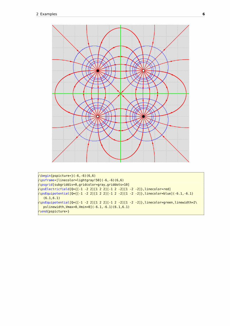
1\begin{pspicture*}(-6,-6)(6,6)2\psframe*[linecolor=lightgray!50](-6,-6)(6,6)3\psgrid[subgriddiv=0,gridcolor=gray,griddots=10]4\psElectricfield[Q={[-1 -2 2][1 2 2][-1 2 -2][1 -2 -2]},linecolor=red]5\psEquipotential[Q={[-1 -2 2][1 2 2][-1 2 -2][1 -2 -2]},linecolor=blue](-6.1,-6.1)

(6.1,6.1)6\psEquipotential[Q={[-1 -2 2][1 2 2][-1 2 -2][1 -2 -2]},linecolor=green,linewidth=2\

pslinewidth,Vmax=0,Vmin=0](-6.1,-6.1)(6.1,6.1)7\end{pspicture*}

2 Examples 7

1\begin{pspicture*}(-6,-6)(6,6)2\psframe*[linecolor=lightgray!50](-6,-6)(6,6)3\psgrid[subgriddiv=0,gridcolor=gray,griddots=10]4\psElectricfield[Q={[-1 -2 2 false][1 2 2 false][-1 2 -2 false][1 -2 -2 false]},radius

=1.5pt,linecolor=red]5\psEquipotential[Q={[-1 -2 2][1 2 2][-1 2 -2][1 -2 -2]},linecolor=blue](-6,-6)(6,6)6\psEquipotential[Q={[-1 -2 2][1 2 2][-1 2 -2][1 -2 -2]},linecolor=green,linewidth=2\

pslinewidth,Vmax=0,Vmin=0](-6.1,-6.1)(6.1,6.1)7\end{pspicture*}

2 Examples 8

1\begin{pspicture*}(-5,-5)(5,5)2\psframe*[linecolor=lightgray!40](-5,-5)(5,5)3\psgrid[subgriddiv=0,gridcolor=lightgray,griddots=10]4\psElectricfield[Q={[-1 -3 1][1 1 -3][-1 2 2]},N=9,linecolor=red,points=1000,posArrow

=0.1,Pas=0.015]5\psEquipotential[Q={[-1 -3 1][1 1 -3][-1 2 2]},linecolor=blue](-6,-6)(6,6)6\psEquipotential[Q={[-1 -3 1][1 1 -3][-1 2 2]},linecolor=green,Vmin=-5,Vmax=-5,

linewidth=2\pslinewidth](-6,-6)(6,6)7\end{pspicture*}

2 Examples 9

1\begin{pspicture*}(-5,-5)(5,5)2\psframe*[linecolor=green!20](-5,-5)(5,5)3\psgrid[subgriddiv=0,gridcolor=lightgray,griddots=10]4\psElectricfield[Q={[1 -2 0][-1 2 0]},linecolor=red]5\psEquipotential[Q={[1 -2 0][-1 2 0]},linecolor=blue](-5,-5)(5,5)6\psEquipotential[Q={[1 -2 0][-1 2 0]},linecolor=green,Vmin=0,Vmax=0](-5,-5)(5,5)7\end{pspicture*}

2 Examples 10

1\begin{pspicture*}(-5,-5)(5,5)2\psframe*[linecolor=green!20](-5,-5)(5,5)3\psgrid[subgriddiv=0,gridcolor=lightgray,griddots=10]4\psElectricfield[Q={[1 -2 0][1 2 0]},linecolor=red,N=15,points=500]5\psEquipotential[Q={[1 -2 0][1 2 0]},linecolor=blue,Vmin=0,Vmax=20,stepV=2](-5,-5)

(5,5)6\psEquipotential[Q={[1 -2 0][1 2 0]},linecolor=green,Vmin=9,Vmax=9](-5,-5)(5,5)7\end{pspicture*}

2 Examples 11

1\begin{pspicture*}(-10,-5)(6,5)2\psframe*[linecolor=lightgray!40](-10,-5)(6,5)3\psgrid[subgriddiv=0,gridcolor=lightgray,griddots=10]4\psElectricfield[Q={[600 -60 0 false][-4 0 0] },N=50,points=500,runit=0.8]5\psEquipotential[Q={[600 -60 0 false][-4 0 0]},linecolor=blue,Vmax=100,Vmin=50,stepV

=2](-10,-5)(6,5)6\psframe*(-10,-5)(-9.5,5)7\rput(0,0){\textcolor{white}{\large$-$}}8\multido{\rA=4.75+-0.5}{20}{\rput(-9.75,\rA){\textcolor{white}{\large$+$}}}9\end{pspicture*}

2 Examples 12

1\begin{pspicture*}(-5,-5)(5,5)2\psframe*[linecolor=green!20](-6,-5)(6,5)3\psgrid[subgriddiv=0,gridcolor=lightgray,griddots=10]4\psElectricfield[Q={[1 -2 -2][1 -2 2][1 2 2][1 2 -2]},linecolor={[HTML]{006633}}]5\psEquipotential[Q={[1 -2 -2][1 -2 2][1 2 2][1 2 -2]},Vmax=15,Vmin=0,stepV=1,linecolor

=blue](-6,-6)(6,6)6\end{pspicture*}

2 Examples 13

1\begin{pspicture*}(-5,-5)(5,5)2\psframe*[linecolor=green!20](-5,-5)(5,5)3\psgrid[subgriddiv=0,gridcolor=lightgray,griddots=10]4\psElectricfield[Q={[1 2 0][1 1 1.732][1 -1 1.732][1 -2 0][1 -1 -1.732][1 1 -1.732]},

linecolor=red]5\psEquipotential[Q={[1 2 0][1 1 1.732 12][1 -1 1.732][1 -2 0][1 -1 -1.732][1 1

-1.732]},linecolor=blue,Vmax=50,Vmin=0,stepV=5](-5,-5)(5,5)6\end{pspicture*}

2 Examples 14

1\begin{pspicture*}(-5,-5)(5,5)2\psframe*[linecolor=green!20](-5,-5)(5,5)3\psgrid[subgriddiv=0,gridcolor=lightgray,griddots=10]4\psElectricfield[Q={[1 2 0][1 1 1.732][1 -1 1.732][1 -2 0][1 -1 -1.732][1 1 -1.732][-1

0 0]},linecolor=red]5\psEquipotential[Q={[1 2 0][1 1 1.732 12][1 -1 1.732][1 -2 0][1 -1 -1.732][1 1

-1.732][-1 0 0]},Vmax=40,Vmin=-10,stepV=5,linecolor=blue](-5,-5)(5,5)6\end{pspicture*}

2 Examples 15

1\begin{pspicture*}(-6,-5)(6,5)2\psframe*[linecolor=green!20](-6,-5)(6,5)3\psgrid[subgriddiv=0,gridcolor=lightgray,griddots=10]4\psElectricfield[Q={[1 -4 0][1 -2 0 12][1 0 0][1 2 0][1 4 0]},linecolor=red]5\psEquipotential[Q={[1 -4 0][1 -2 0][1 0 0][1 2 0][1 4 0]},linecolor=blue,Vmax=30,Vmin

=0,stepV=2](-7,-5)(7,5)6\end{pspicture*}

References 16

3 List of all optional arguments for pst-electricfield

Key Type Default

Q ordinary [1 -2 0 10][1 1 0][1 0 1 15]N ordinary 17points ordinary 400Pas ordinary 0.025posArrow ordinary [none]Vmax ordinary 10Vmin ordinary -10stepV ordinary 2stepFactor ordinary 0.67

References

[1] M. Abramowitz and I. A. Stegun. Handbook of Mathematical Functions withFormulas, Graphs, and Mathematical Tables. National Bureau of StandardsApplied Mathematics Series, U.S. Government Printing Office, Washington, D.C.,USA, 1964. Corrections appeared in later printings up to the 10th Printing.

[2] Denis Girou. Présentation de PSTricks. Cahier GUTenberg, 16:21–70, April 1994.

[3] Michel Goosens, Frank Mittelbach, Sebastian Rahtz, Dennis Roegel, and HerbertVoß. The LATEX Graphics Companion. Addison-Wesley Publishing Company,Reading, Mass., second edition, 2007.

[4] Nikolai G. Kollock. PostScript richtig eingesetzt: vom Konzept zum praktischenEinsatz. IWT, Vaterstetten, 1989.

[5] Dolan Thomas J. Fusion Research, Volume III “Technology”. Pergamon Press,1982. Chapter 20 “Water-cooled magnets” , pages 600 ff “circular loops” –Integrating the Biot-Savart Law (in cylindrical geometry).

[6] Herbert Voß. PSTricks – Grafik für TEX und LATEX. DANTE – Lehmanns,Heidelberg/Hamburg, fifth edition, 2008.

[7] Timothy Van Zandt. multido.tex - a loop macro, that supports fixed-point addition.CTAN:/graphics/pstricks/generic/multido.tex, 1997.

[8] Timothy Van Zandt and Denis Girou. Inside PSTricks. TUGboat, 15:239–246,September 1994.

Index

MMacro– \psplotImp, 2

PPackage– pst-func, 2\psplotImp, 2pst-func, 2

17