psych 230 statistics - university of...
TRANSCRIPT
1
PSYCH 230 – STATISTICS
1) If you are already registered sit down.
2) If you are on the waiting list or just showed up,
stay standing and we will see how many seats are
available.
3) We will start adding using the waiting list.

2
PSYCHOLOGY 230 - STATS
Elizabeth Krupinski, PhD
Depts. Radiology & Psychology
112 Radiology Research Building
626-4498
http://krupinski.radiology.arizona.edu/psych230.htm
3
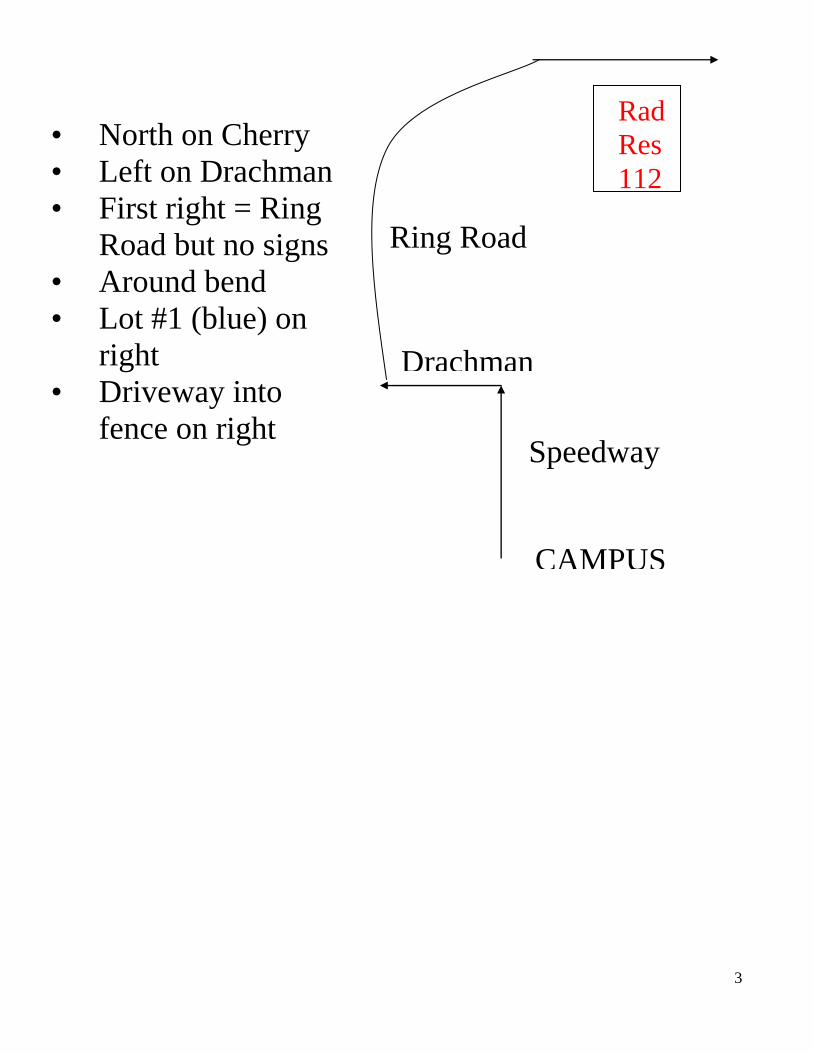
CAMPUS
• North on Cherry
• Left on Drachman
• First right = Ring
Road but no signs
• Around bend
• Lot #1 (blue) on
right
• Driveway into
fence on right
• Radiology
Research Bldg
• Room 112
Rad
Res
112
Speedway
Drachman
Ring Road
4
PREREQUISITES
1) Psych 101 or IND 101
2) Math 110 – college algebra
+, x, -, ÷, √, , , | |
positive vs negative numbers
order of operations
rounding: < 5 down, > 5 up
decimals: 2 places on quizzes
5
QUIZZES
4 quizzes
- each 25% of your grade
- 100 points each
- all of them count (none dropped)
~ 1/3 fill-in-the-blank
- comprehension of concepts
- ability to apply principles, terms, etc.
~ 2/3 problems
- ability identify appropriate equations
- ability carry out required math
- ability use statistical tables
- ability reach proper conclusions
formulas & tables provided on quizzes
6
EXTRA CREDIT
1) Hand in a MAXIMUM of 5 completed
homework assignments - 1 point each - 5 points
maximum (hand in all 5 at once)
2) Hand in completed worksheet packet at end of
semester - 10 points
3) Find a journal article with statistics in it; in 3
pages explain the statistics - why used, what tests,
interpret etc. - 10 points
15 POINTS MAXIMUM!!!!!!
Final grade = (4 quiz grades + extra credit)/4
7
TEXTS
Class notes: buy in the bookstore (required)
http://www.radiology.arizona.edu/krupinski/index.html
Book: Fundamentals of Behavioral Statistics
9th
edition
Runyon, Coleman & Pittenger (optional)

8
CALCULATORS
DO NOT FORGET TO BRING YOUR
CALCULATOR TO THE QUIZZES!!!!!!
Required:
+, -, x, ,
Helpful:
X (sometimes )- mean
S (SD) - standard deviation (sometimes is )
X - sum X
X2 - sum X squared
N or n – number

9
BASIC MATH REVIEW
2 + 2 = 4
2 + (-2) = 0
(-2) + (-2) = (-4)
2 x 2 = 4
2 x (-2) = (-4)
(-2) x (-2) = 4
2 – 2 = 0
2 – (-2) = 4
(-2) – (-2) = 0
2/2 = 1
2/(-2) = (-1)
(-2)/(-2) = 1
22 = 4
(-2)2 = 4
√4 = 2
√(-4) = error

10
+ +
+ -
- +
_ _
GRAPHING QUADRANTS
11
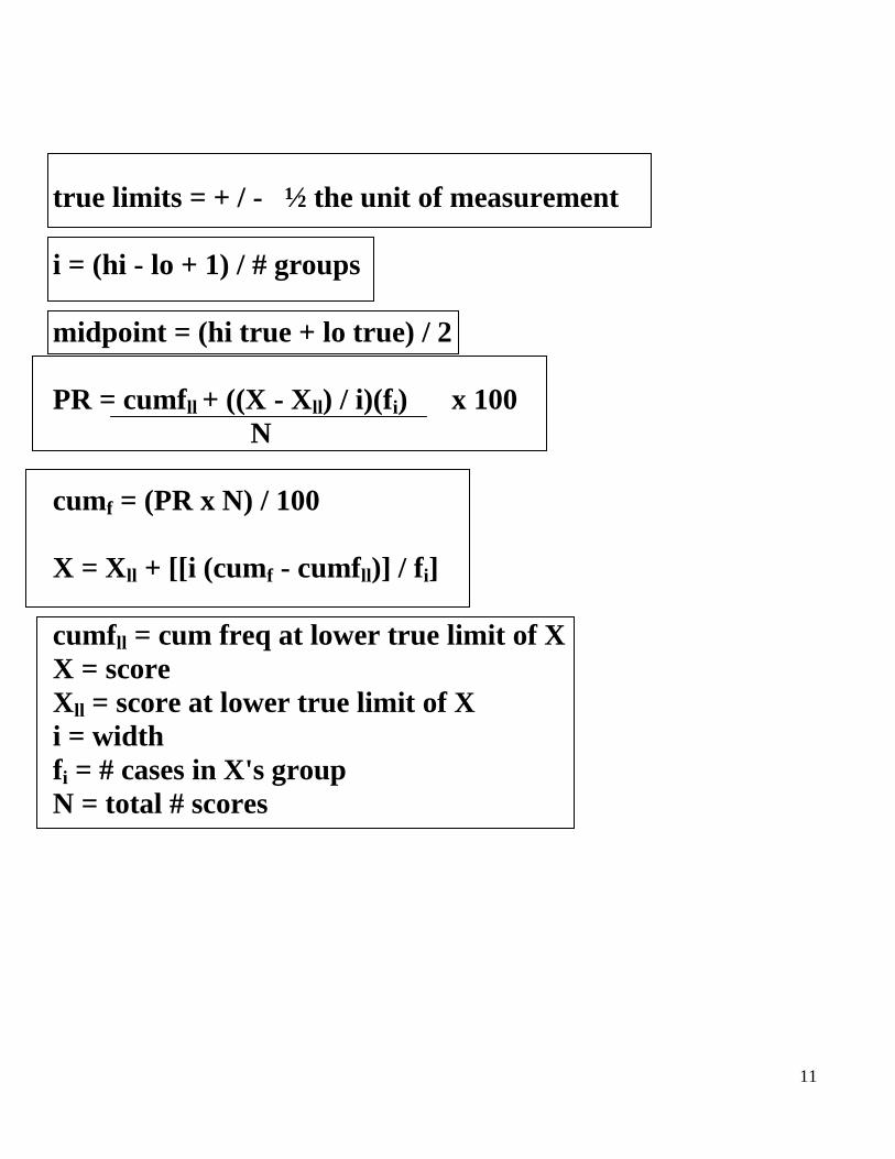
true limits = + / - ½ the unit of measurement
i = (hi - lo + 1) / # groups
midpoint = (hi true + lo true) / 2
PR = cumfll + ((X - Xll) / i)(fi) x 100
N
cumf = (PR x N) / 100
X = Xll + [[i (cumf - cumfll)] / fi]
cumfll = cum freq at lower true limit of X
X = score
Xll = score at lower true limit of X
i = width
fi = # cases in X's group
N = total # scores

12
- Sam wants to find out if the number of hours
people study has any effect on their grade.
- Mary wants to find out if gender has any
influence on math and verbal SAT scores.
- Dr. Jones wants to find out if her current class
performs any differently on the final compared to
all past students.
- A large pharmaceutical company wants to know
if their new drug for controlling OCD is effective.
13
Chapter 1: What is statistics?
- statistics: the process of collecting data & making decisions
based on the analysis of these data
descriptive inferential (generalize)
Common Terms
- constant: # representing a construct that does not change
(e.g., ); we will see these in some formulas
- variable: measurable characteristic that changes with
person, environment, experiment e.g., height, IQ, learning
(X or Y)
- independent variable (IV): variable examined to determine
its effect on outcome of interest (DV); under control of
experimenter - manipulated variable; e.g., dose of a drug
- dependent variable (DV): outcome of interest measured to
assess effects of IV; not under experimenter control; e.g.,
how a person reacts to the drug
- subject or organismic variable: naturally occurring IV;
characteristic of people but not controlled e.g., eye color,
gender

14
- data: numbers, measurements collected
- population: complete set of people/objects having some
common characteristic
- parameter: value summarizing characteristic of
population; are constants; use Greek letters to represent
- sample: subset of population, share same characteristics
- statistic: value summarizing characteristic of a sample; are
variable; use Roman letters to represent
- simple random sample: subset of population selected so that
each population member has = & independent chance of
being chosen
- random assignment: assign subjects to treatments in = &
independent manner to avoid bias
- confounding: where DV is affected by variable related to IV
so can't assume that IV causes DV effects
15
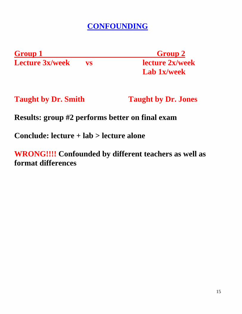
CONFOUNDING
Group 1 Group 2
Lecture 3x/week vs lecture 2x/week
Lab 1x/week
Taught by Dr. Smith Taught by Dr. Jones
Results: group #2 performs better on final exam
Conclude: lecture + lab > lecture alone
WRONG!!!! Confounded by different teachers as well as
format differences

16
CHAPTER #1 HOMEWORK
1 a-e
3 a-g
4, 6-11
13 a-j
17
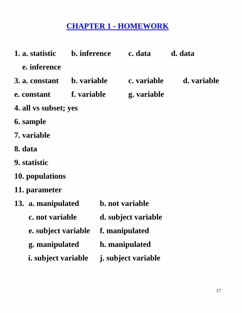
CHAPTER 1 - HOMEWORK
1. a. statistic b. inference c. data d. data
e. inference
3. a. constant b. variable c. variable d. variable
e. constant f. variable g. variable
4. all vs subset; yes
6. sample
7. variable
8. data
9. statistic
10. populations
11. parameter
13. a. manipulated b. not variable
c. not variable d. subject variable
e. subject variable f. manipulated
g. manipulated h. manipulated
i. subject variable j. subject variable
18
- Fred wants to find out what types of pets college students
have.
- Alice wants to find out if birth order has any effect on
GPA.
- Mike wants to look at temperature effects on ice cream
consumption.
- Sally wants to see how fast rats run through a maze as a
function of reward type at the end.
- Rick wants to examine how many kids people have today
compared to 50 years ago.
- Mary wants to examine how tall people are compared to 50
years ago.

19
Chapter 2 - Basic Concepts
- X or Y: symbol for a variable
- Xi or Yi: represents individual observation
- N or n: # data points in a set, number
- : indicates summation
EXAMPLES (X = group 1 kids, y = group 2 kids)
X1 = 4 X2 = 6 X3 = 1 X4 = 5 X5 = 2 X6 = 3
Y1 = 3 Y2 = 4 Y3 = 6 Y4 = 1
a) Xi = 1 + 5 + 2 + 3 = 11
b) Yi = 3 + 4 + 6 = 13
* c) Xi2 = 5
2 + 2
2 + 3
2 = 25 + 4 + 9 = 38
* d) ( Xi)2 = (5 + 2 + 3)
2 = 10
2 = 100
e) Xi = 6 + 1 + 5 + 2 + 3 = 17
N = go to the end; use all #s from start point
6
i = 3
3
i = 1
6
i = 4
6
i = 4
N
i = 2
NOT THE
SAME !!!!
Where you stop
Where you start
20
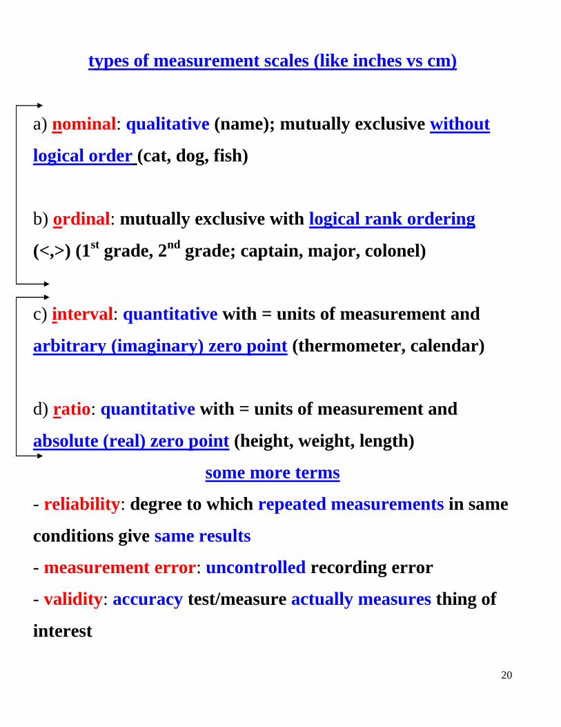
types of measurement scales (like inches vs cm)
a) nominal: qualitative (name); mutually exclusive without
logical order (cat, dog, fish)
b) ordinal: mutually exclusive with logical rank ordering
(<,>) (1st grade, 2
nd grade; captain, major, colonel)
c) interval: quantitative with = units of measurement and
arbitrary (imaginary) zero point (thermometer, calendar)
d) ratio: quantitative with = units of measurement and
absolute (real) zero point (height, weight, length)
some more terms
- reliability: degree to which repeated measurements in same
conditions give same results
- measurement error: uncontrolled recording error
- validity: accuracy test/measure actually measures thing of
interest
21
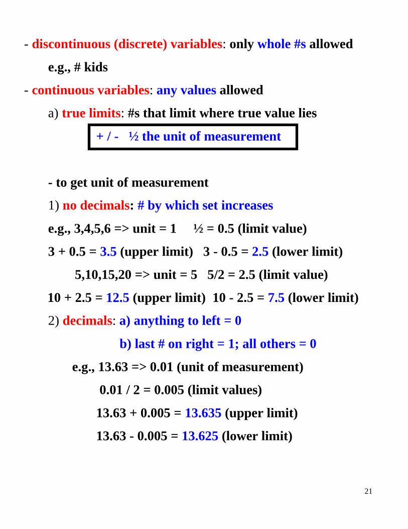
- discontinuous (discrete) variables: only whole #s allowed
e.g., # kids
- continuous variables: any values allowed
a) true limits: #s that limit where true value lies
+ / - ½ the unit of measurement
- to get unit of measurement
1) no decimals: # by which set increases
e.g., 3,4,5,6 => unit = 1 ½ = 0.5 (limit value)
3 + 0.5 = 3.5 (upper limit) 3 - 0.5 = 2.5 (lower limit)
5,10,15,20 => unit = 5 5/2 = 2.5 (limit value)
10 + 2.5 = 12.5 (upper limit) 10 - 2.5 = 7.5 (lower limit)
2) decimals: a) anything to left = 0
b) last # on right = 1; all others = 0
e.g., 13.63 => 0.01 (unit of measurement)
0.01 / 2 = 0.005 (limit values)
13.63 + 0.005 = 13.635 (upper limit)
13.63 - 0.005 = 13.625 (lower limit)

22
some basic descriptive statistics
1) frequency: count
class = 20 13 women; 7 men
2) ratio: 13:7 women to men; DO NOT REDUCE
20: 5 do not reduce to 4:1
3) proportion: fraction 13/20 = 0.65 women
DO OUT THE DIVISION
4) percentage: proportion x 100 7/20 x 100 = 35% men
23
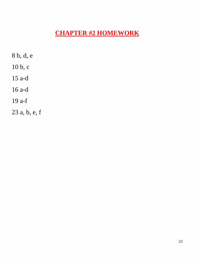
CHAPTER #2 HOMEWORK
8 b, d, e
10 b, c
15 a-d
16 a-d
19 a-f
23 a, b, e, f
24
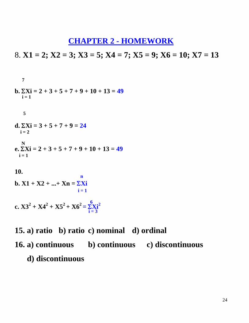
CHAPTER 2 - HOMEWORK
8. X1 = 2; X2 = 3; X3 = 5; X4 = 7; X5 = 9; X6 = 10; X7 = 13
b. Xi = 2 + 3 + 5 + 7 + 9 + 10 + 13 = 49
d. Xi = 3 + 5 + 7 + 9 = 24
e. Xi = 2 + 3 + 5 + 7 + 9 + 10 + 13 = 49
10.
b. X1 + X2 + ...+ Xn = Xi
c. X32 + X4
2 + X5
2 + X6
2 = Xi
2
15. a) ratio b) ratio c) nominal d) ordinal
16. a) continuous b) continuous c) discontinuous
d) discontinuous
5
7
i = 1
i = 2
N
i = 1
n
i = 1
6
i = 3
25
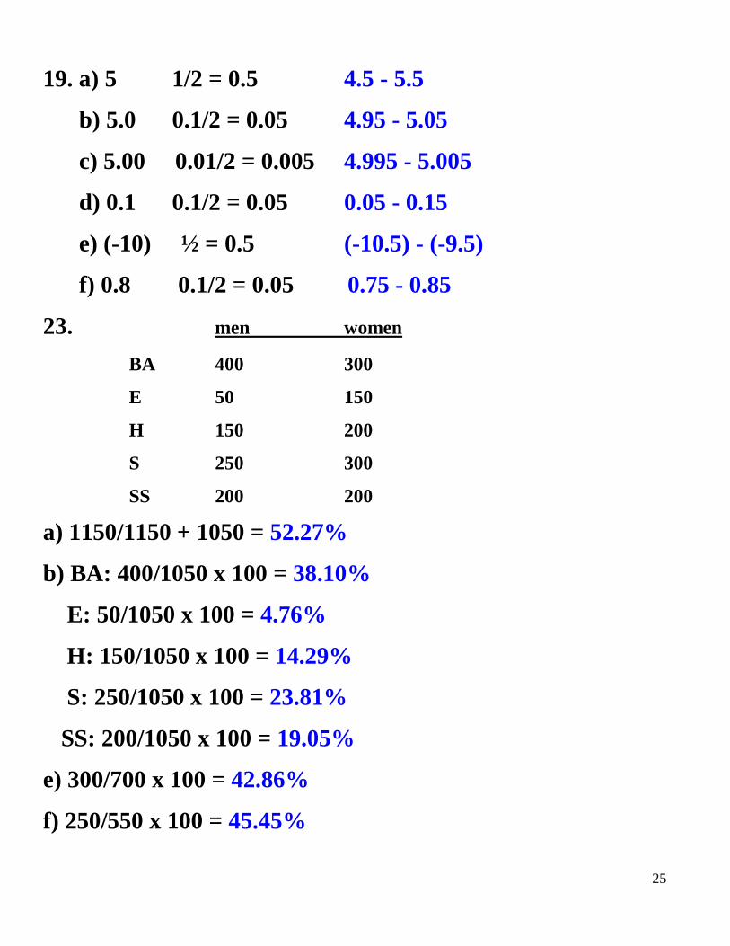
19. a) 5 1/2 = 0.5 4.5 - 5.5
b) 5.0 0.1/2 = 0.05 4.95 - 5.05
c) 5.00 0.01/2 = 0.005 4.995 - 5.005
d) 0.1 0.1/2 = 0.05 0.05 - 0.15
e) (-10) ½ = 0.5 (-10.5) - (-9.5)
f) 0.8 0.1/2 = 0.05 0.75 - 0.85
23. men women
BA 400 300
E 50 150
H 150 200
S 250 300
SS 200 200
a) 1150/1150 + 1050 = 52.27%
b) BA: 400/1050 x 100 = 38.10%
E: 50/1050 x 100 = 4.76%
H: 150/1050 x 100 = 14.29%
S: 250/1050 x 100 = 23.81%
SS: 200/1050 x 100 = 19.05%
e) 300/700 x 100 = 42.86%
f) 250/550 x 100 = 45.45%
26
- I have 23,184 data points from my experiment - what do I
do with all that information?
- How do I present that information to someone else?
- Mitch got a 43 on the quiz – how did he do compared to
everyone else?
- Ann was told she scored at the 75th
percentile on the GRE
exam – what does that mean?
27
1325.000 FN one 1445.000 FP one 2316.000 FP one
1152.000 FN one 1298.000 FN one 1876.000 FP one
945.000 FN one 905.000 FN one 675.000 FN one
1273.000 TP one 396.000 FN one 1007.000 FN one
1378.000 TP one 1267.000 TP one 1267.000 FN one
945.000 TP one 1432.000 TP one 540.000 FN one
1106.000 TP one 1765.000 TP one 1765.000 TP one
1258.000 TP one 1546.000 TP one 1549.000 TP one
734.000 TP one 1653.000 TP one 1289.000 TP one
1569.000 TP one 907.000 TP one 2006.000 TP one
1328.000 TP one 1167.000 TP one 2176.000 TP one
1741.000 TP one 1659.000 TP one 1894.000 TP one
1143.000 TP one 1734.000 TP one 1856.000 TP one
2003.000 TP one 1178.000 TP one 1287.000 TP one
1475.000 TP one 1342.000 TP one 1089.000 TP one
967.000 FP two 1976.000 TP one 2108.000 TP one
1263.000 FN two 1386.000 FP two 765.000 TP one
1367.000 TP two 890.000 FN two 1492.000 FP two
945.000 TP two 1239.000 FN two 1167.000 FP two
824.000 TP two 1643.000 TP two 2076.000 FP two
1428.000 TP two 1128.000 TP two 1750.000 FN two
1184.000 TP two 1378.000 TP two 230.000 FN two
1205.000 TP two 1785.000 TP two 1437.000 TP two
1428.000 TP two 1675.000 TP two 2178.000 TP two
947.000 TP two 1429.000 TP two 1856.000 TP two
723.000 TP two 1167.000 TP two 298.000 TP two
1132.000 TP two 1745.000 TP two 1429.000 TP two
1639.000 TP two 1067.000 TP two 1763.000 TP two
1174.000 TP two 945.000 TP two 1967.000 TP two
1002.000 TP two 1858.000 TP two 3012.000 TP two
1421.000 TP two 1428.000 TP two 1865.000 TP two
1167.000 FP three 1745.000 TP two 670.000 TP two

28
905.000 FN three 2067.000 FP three 1654.000 TP two
1427.000 TP three 1004.000 FN three 1865.000 TP two
1538.000 TP three 1538.000 TP three 1896.000 TP two
1142.000 TP three 1843.000 TP three 1267.000 FP three
1632.000 TP three 1178.000 TP three 2006.000 FP three
1189.000 TP three 1906.000 TP three 1290.000 FN three
564.000 TP three 507.000 TP three 543.000 FN three
1195.000 TP three 1427.000 TP three 1100.000 FN three
1427.000 TP three 1778.000 TP three 956.000 FN three
1894.000 TP three 1638.000 TP three 1785.000 TP three
792.000 TP three 1324.000 TP three 1098.000 TP three
1063.000 TP three 1756.000 TP three 1278.000 TP three
1217.000 TP three 1542.000 TP three 1850.000 TP three
1853.000 TP three 1008.000 TP three 1645.000 TP three
904.000 TP three 1105.000 TP three 1238.000 TP three
1648.000 FP four 788.000 TP three 786.000 TP three
1284.000 FP four 1267.000 FP four 1278.000 TP three
1202.000 FN four 1867.000 FN four 1956.000 TP three
2548.000 FN four 238.000 FN four 1673.000 TP three
1732.000 TP four 1427.000 TP four 1978.000 TP three
894.000 TP four 1867.000 TP four 2156.000 FP four
1263.000 TP four 2067.000 TP four 967.000 FP four
1048.000 TP four 1967.000 TP four 1785.000 FN four
1723.000 TP four 1754.000 TP four 1267.000 FN four
604.000 TP four 1329.000 TP four 906.000 FN four
2004.000 TP four 1867.000 TP four 397.000 FN four
793.000 TP four 1540.000 TP four 1056.000 FN four
1174.000 TP four 1756.000 TP four 529.000 FN four
1631.000 TP four 1230.000 TP four 567.000 TP four
1060.000 TP four 905.000 TP four 1275.000 TP four
1428.000 TP four 1976.000 TP four 1845.000 TP four
956.000 TP four 1056.000 TP four 1834.000 TP four
29
1639.000 FP five 905.000 FP five 1839.000 TP four
1067.000 FN five 1276.000 FN five 2004.000 TP four
1284.000 FN five 670.000 FN five 568.000 TP four
954.000 TP five 1078.000 FN five 1745.000 TP four
1743.000 TP five 1649.000 TP five 1954.000 TP four
1184.000 TP five 1978.000 TP five 1789.000 FP five
1630.000 TP five 2005.000 TP five 452.000 FN five
1007.000 TP five 1967.000 TP five 1169.000 FN five
584.000 TP five 1286.000 TP five 2006.000 FN five
1639.000 TP five 1095.000 TP five 1759.000 FN five
1075.000 TP five 1745.000 TP five 1278.000 TP five
945.000 TP five 2006.000 TP five 1948.000 TP five
1006.000 TP five 670.000 TP five 1739.000 TP five
569.000 TP five 1750.000 TP five 1237.000 TP five
1197.000 TP five 2967.000 TP five 187.000 TP five
1143.000 TP five 1756.000 TP five 1854.000 TP five
904.000 FP six 1267.000 FP six 2068.000 TP five
1211.000 FN six 905.000 FP six 2178.000 TP five
1406.000 FN six 2078.000 FN six 1762.000 TP five
1134.000 TP six 1956.000 FN six 906.000 TP five
783.000 TP six 1328.000 TP six 2170.000 TP five
1290.000 TP six 567.000 TP six 3001.000 FP six
1329.000 TP six 1967.000 TP six 1275.000 FP six
605.000 TP six 2865.000 TP six 1967.000 FN six
1468.000 TP six 1856.000 TP six 238.000 FN six
1126.000 TP six 459.000 TP six 911.000 FN six
1390.000 TP six 1853.000 TP six 1765.000 TP six
685.000 TP six 1953.000 TP six 507.000 TP six
1056.000 TP six 1956.000 TP six 1176.000 TP six
1265.000 TP six 2006.000 TP six 1967.000 TP six
2006.000 TP six 1654.000 TP six 1659.000 TP six
1421.000 TP six 609.000 TP six 2002.000 TP six

30
Chapter 3 - Frequency Distributions & Percentiles
- exploratory data analysis: ways to arrange & display #s to
quickly organize & summarize data
- grouping data
1) frequency distribution: high - low
pet type frequency proportion %
dog 20 0.43 (20/46) 43.00 (0.43 x 100)
cat 15 0.33 33.00
turtle 11 0.24 24.00
46 1.00 100.00
2) grouping in classes
a) aim for 12 - 15 groups
b) mutually exclusive
c) same width
d) don't omit intervals
e) make widths convenient
width = (hi - lo + 1) / # groups = i
31
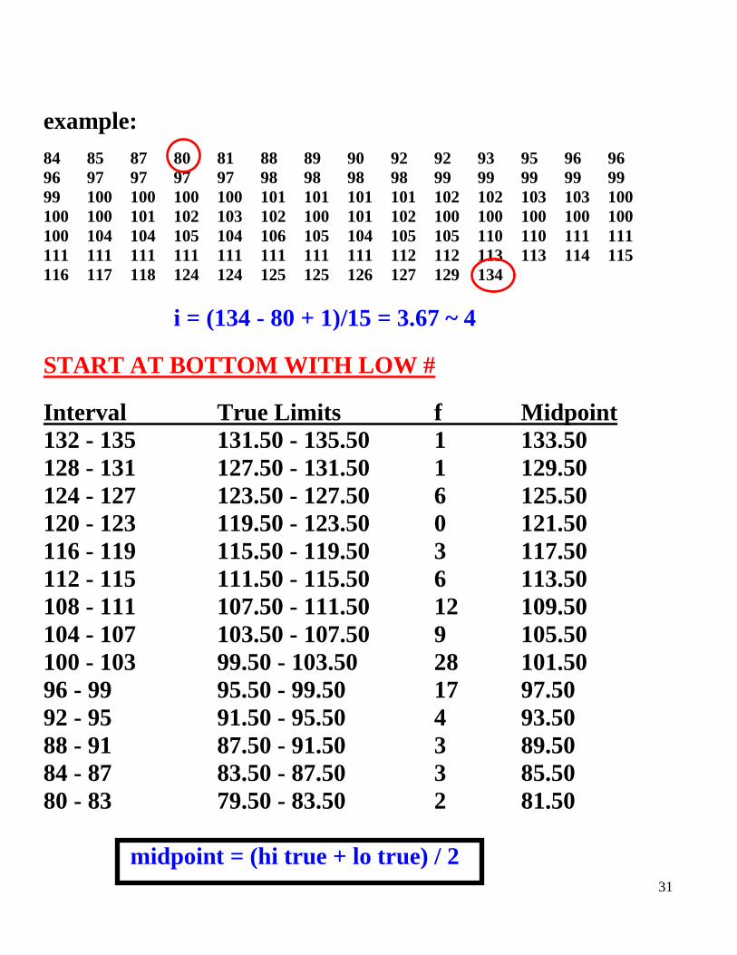
example:
84 85 87 80 81 88 89 90 92 92 93 95 96 96
96 97 97 97 97 98 98 98 98 99 99 99 99 99
99 100 100 100 100 101 101 101 101 102 102 103 103 100
100 100 101 102 103 102 100 101 102 100 100 100 100 100
100 104 104 105 104 106 105 104 105 105 110 110 111 111
111 111 111 111 111 111 111 111 112 112 113 113 114 115
116 117 118 124 124 125 125 126 127 129 134
i = (134 - 80 + 1)/15 = 3.67 ~ 4
START AT BOTTOM WITH LOW #
Interval True Limits f Midpoint
132 - 135 131.50 - 135.50 1 133.50
128 - 131 127.50 - 131.50 1 129.50
124 - 127 123.50 - 127.50 6 125.50
120 - 123 119.50 - 123.50 0 121.50
116 - 119 115.50 - 119.50 3 117.50
112 - 115 111.50 - 115.50 6 113.50
108 - 111 107.50 - 111.50 12 109.50
104 - 107 103.50 - 107.50 9 105.50
100 - 103 99.50 - 103.50 28 101.50
96 - 99 95.50 - 99.50 17 97.50
92 - 95 91.50 - 95.50 4 93.50
88 - 91 87.50 - 91.50 3 89.50
84 - 87 83.50 - 87.50 3 85.50
80 - 83 79.50 - 83.50 2 81.50
midpoint = (hi true + lo true) / 2

32
- cumulative data
class grades f cum f cum prop cum %
91 - 100 6 32 1.00 100.00
81 - 90 4 26 0.8125 81.25
71 - 80 9 22 0.6875 68.75
61-70 11 13 0.4062 40.62
51 - 60 2 2 0.0625 6.25
32
Percentiles & Percentile Ranks
- score alone means nothing, must compare to standard or
base score; can do with percentiles
- percentiles: #s that divide distribution into 100 = parts
- percentile rank: # that represents the % of cases in a
comparison group that achieved scores < the one cited
e.g., PR of 95 on SAT means 95% of those taking SAT at the
same time did worse than you & 5% did better
some symbols
cumfll = cum freq at lower true limit of X
X = score
Xll = score at lower true limit of X
i = width
fi = # cases in X's group
N = total # scores

33
1) Getting PR from score (X)
PR = cumfll + ((X - Xll)/i) (fi) x 100
N
Class (X) limits f cum f cum %
93 - 95 92.50 - 95.50 4 25 100.00
90 - 92 89.50 - 92.50 3 21 84.00
87 - 89 86.50 - 89.50 2 18 72.00
84 - 86 83.50 - 86.50 7 16 64.00
81 - 83 80.50 - 83.50 6 9 36.00
78 - 80 77.50 - 80.50 3 3 12.00
What is PR of 88?
X = 88
cumfll = 16
Xll = 86.5
i = 3
fi = 2
N = 25
NB: PR goes from 0 – 100
PR = 16 + ((88 - 86.50) / 3) (2) x 100
25
PR = 68
34
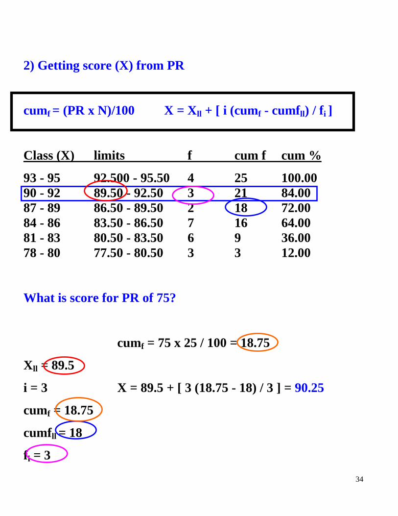
2) Getting score (X) from PR
cumf = (PR x N)/100 X = Xll + [ i (cumf - cumfll) / fi ]
Class (X) limits f cum f cum %
93 - 95 92.500 - 95.50 4 25 100.00
90 - 92 89.50 - 92.50 3 21 84.00
87 - 89 86.50 - 89.50 2 18 72.00
84 - 86 83.50 - 86.50 7 16 64.00
81 - 83 80.50 - 83.50 6 9 36.00
78 - 80 77.50 - 80.50 3 3 12.00
What is score for PR of 75?
cumf = 75 x 25 / 100 = 18.75
Xll = 89.5
i = 3 X = 89.5 + [ 3 (18.75 - 18) / 3 ] = 90.25
cumf = 18.75
cumfll = 18
fi = 3

35
CHAPTER 3 HOMEWORK
3 a - use 18 for # groups
3b
c – not in book – What is PR if X = 36 using data from # 3
d – not in book – What is X if PR = 09? Use data from # 3

36
CHAPTER 3 - HOMEWORK
3 a) if you want 18 groups: (90 - 5 + 1) / 18 = 4.7 ~ 5
b) group limits mdpt f cumf cum%
90 - 94 89.50 - 94.50 92 1 90 100.00
85 - 89 84.50 - 89.50 87 0 89 98.89
80 - 84 79.50 - 84.50 82 0 89 98.89
75 - 79 74.50 - 79.50 77 1 89 98.89
70 - 74 69.50 - 74.50 72 0 88 97.78
65 - 69 64.50 - 69.50 67 3 88 97.78
60 - 64 59.50 - 64.50 62 4 85 94.44
55 - 59 54.50 - 59.50 57 7 81 90.00
50 - 54 49.50 - 54.50 52 5 74 82.22
45 - 49 44.50 - 49.50 47 11 69 76.67
40 - 44 39.50 - 44.50 42 11 58 64.44
35 - 39 34.50 - 39.50 37 10 47 52.22
30 - 34 29.50 - 34.50 32 9 37 41.11
25 - 29 24.50 - 29.50 27 8 28 31.11
20 - 24 19.50 - 24.50 22 5 20 22.22
15 - 19 14.50 - 19.50 17 9 15 16.67
10 - 14 9.50 - 14.50 12 4 6 6.67
5 - 9 4.50 - 9.50 7 2 2 2.22
c) what is PR if X = 36?
PR = 37 + ((36 - 34.50) / 5) (10) x 100 = 44.44
90
d) what is X if PR = 98?
cumf = 98 x 90 / 100 = 88.20
X = 74.50 + [ 5 (88.2 - 88) / 1 ] = 75.50

37
- What types of graphs are used most often in psychology?
- Are there rules for which one to use?
- Are there rules about how to make them?
- Does the shape of the graph mean anything useful?

38
Chapter 7 - Graphing
- visual methods to display data
a) figure: pictorial; photo, drawing
b) table: organized numerical info
c) graph: pictorial; axes, #s etc.
- basics of graphing
a) X-axis (abscissa): horizontal; IV
b) Y-axis (ordinate): vertical; DV
c) always label axes – note the units
d) Y starts at 0; continuous, no breaks
X can change start; break; can be discrete
e) Y about 0.75 length of X
1) Bar Graph: nominal, sometimes ordinal
a) bar = category
b) height = frequency
c) bars DO NOT touch
d) if ordinal must preserve order
e) can be vertical or horizontal
0
2
4
6
8
10
12
14
16
18
20
Fre
qu
en
cy
DOG CAT FISH BIRD
Women
Men
Pet w m
Dog 20 10
Cat 15 15
Fish 8 5
Bird 5 14
TYPE OF PET
39
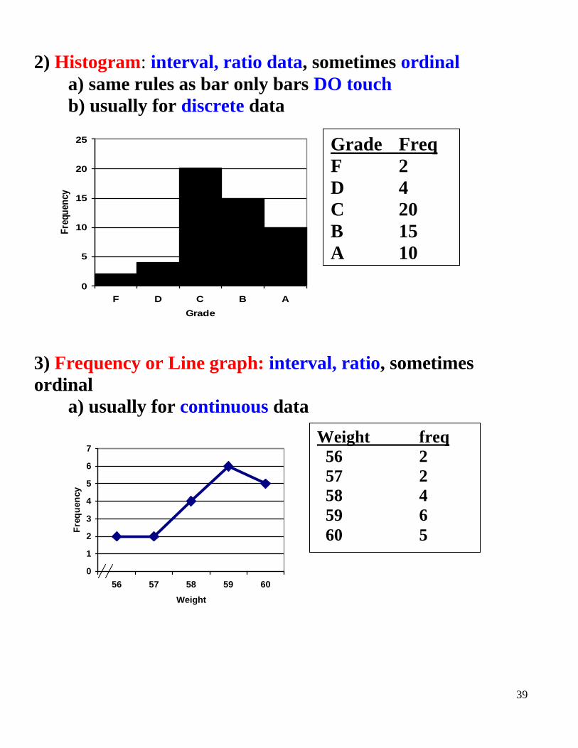
2) Histogram: interval, ratio data, sometimes ordinal
a) same rules as bar only bars DO touch
b) usually for discrete data
3) Frequency or Line graph: interval, ratio, sometimes
ordinal
a) usually for continuous data
0
5
10
15
20
25
F D C B A
Grade
Fre
quen
cy
Grade Freq
F 2
D 4
C 20
B 15
A 10
0
1
2
3
4
5
6
7
56 57 58 59 60
Weight
Fre
qu
en
cy
Weight freq
56 2
57 2
58 4
59 6
60 5

40
4) cumulative frequency: can be bar, histogram or line, but
uses cumulative freq, proportion or %
a) the line graph version is typically s-shaped or ogive
b) always increases
e.g., 12 people on a drug to cure disease X. Left = #
cured each time period. Right = cum % cured over time.
0
0.5
1
1.5
2
2.5
3
3.5
1 3 6 9 12
months on drug
# c
ure
d
0
10
20
30
40
50
60
70
80
1 3 6 9 12
months on drug
Cu
m %
cu
red
Forms of Frequency Curves
1) Normal (bell-shaped) curve: symmetric
a) mesokurtic: ideal
(middle) b) leptokurtic: peaked
(leaping) c) platykurtic: flat
(prairie)
2) skew: not symmetric
a) positive skew: fewer scores at high end;
shifted to left
b) negative skew: fewer scores at low end;
shifted to right

41
CHAPTER 7 HOMEWORK
Chapter 3: 5 a-e
Chapter 7: 7 do 1b
6
7
12 – schizophrenic data only

42
CHAPTER 7 - HOMEWORK
Chap 3 # 5:
a) b) c) d) e)
Chap 7:
1b)
6)
0
2
4
68
10
12
14
16
30-39 40-49 50-59 60-69 70-79 80-89 90-99
scores (midpt)
F
0
10
20
30
40
50
60
70
80
90
100
0 3 6 9 12 15 18
interval (sec)
%

43
7)
12) schizophrenic data only
0
10
20
30
40
50
60
70
1 2 3 4 5 6 7 8 9 10
minutes
F
100%
60%
0
10
20
30
40
50
60
70
80
cat dis par und
type schizophrenia
f

44
z = (X - X) / s = (X - ) /
SIR = (Q3 - Q1) / 2 X = X / n
s
3 = [3(X - median)] / s Range = hi - lo
Xw = fX / ntot
s4 = 3 + [ (Q3 - Q1) / 2 (P90 - P10)]
md = Xll + i [ ((N/2) - cumfll) / fi]
s2 = (X - X)
2 / n s = s
2
SS = X2 - (X)
2/n s
2 = SS/n s = s
2
45
- Sid wants to know what is the average age of people in the
mall before the stores open?
- Dr. Smith has 4 classes each with a different number of
pupils. He has the average grade on the last quiz for each of
the 4 classes but wants to know the overall average.
- If we include all the billionaires in the calculation of the
average US income will it be inflated because of the few very
high values? Is there a better measure than the mean?
46
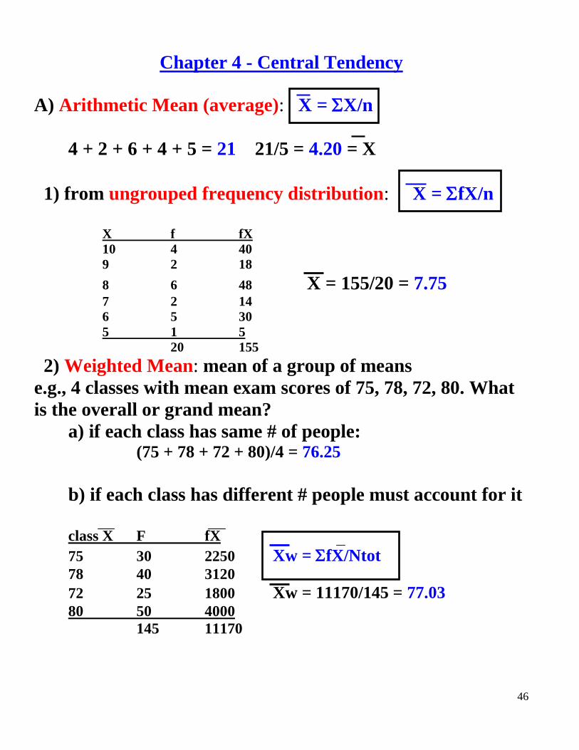
Chapter 4 - Central Tendency
A) Arithmetic Mean (average): X = X/n
4 + 2 + 6 + 4 + 5 = 21 21/5 = 4.20 = X
1) from ungrouped frequency distribution: X = fX/n
X f fX
10 4 40
9 2 18
8 6 48 X = 155/20 = 7.75
7 2 14
6 5 30
5 1 5
20 155 2) Weighted Mean: mean of a group of means
e.g., 4 classes with mean exam scores of 75, 78, 72, 80. What
is the overall or grand mean?
a) if each class has same # of people: (75 + 78 + 72 + 80)/4 = 76.25
b) if each class has different # people must account for it
class X F fX
75 30 2250 Xw = fX/Ntot 78 40 3120
72 25 1800 Xw = 11170/145 = 77.03 80 50 4000
145 11170
47
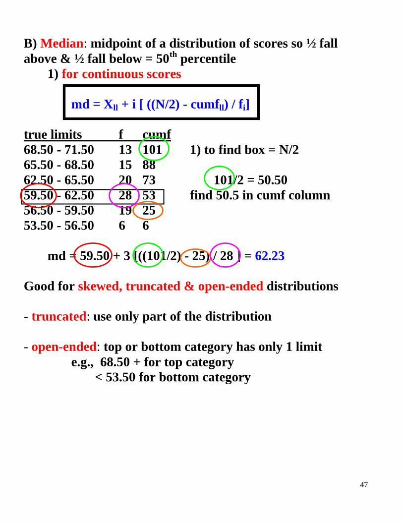
B) Median: midpoint of a distribution of scores so ½ fall
above & ½ fall below = 50th
percentile
1) for continuous scores
md = Xll + i [ ((N/2) - cumfll) / fi]
true limits f cumf
68.50 - 71.50 13 101 1) to find box = N/2
65.50 - 68.50 15 88
62.50 - 65.50 20 73 101/2 = 50.50
59.50 - 62.50 28 53 find 50.5 in cumf column
56.50 - 59.50 19 25
53.50 - 56.50 6 6
md = 59.50 + 3 [((101/2) - 25) / 28 ] = 62.23
Good for skewed, truncated & open-ended distributions
- truncated: use only part of the distribution
- open-ended: top or bottom category has only 1 limit
e.g., 68.50 + for top category
< 53.50 for bottom category

48
2) median for arrays of scores
a) if N is odd => put in ascending order, find middle #
56, 6, 13, 31, 28 => 6, 13, 28, 31, 56
b) if N is even => ascending order, take X of 2 middle #s
6, 13, 28, 31, 56, 72 => (28 + 31) / 2 = 29.50
c) N is even but middle 2 #s are the same => use formula
1, 2, 4, 6, 6, 6, 7, 121
x f cumf
121 1 8 8/2 = 4 => box
7 1 7
6 3 6 md = 5.5 + 1 [ ((8/2) - 3) / 3] = 5.83
4 1 3
2 1 2
1 1 1
C) Mode: most common score; crude measure
1) 1, 3, 4, 6, 7, 7, 7, 9, 9 mode = 7
2, 2, 4, 9, 9 mode = 2, 9
2) class f
68.5 - 71.5 10 1) find highest f value
65.5 - 68.5 15 2) report midpoint as mode
62.5 - 65.5 9
59.5 - 62.5 10 mode = (68.5 + 65.5) / 2 = 67
49
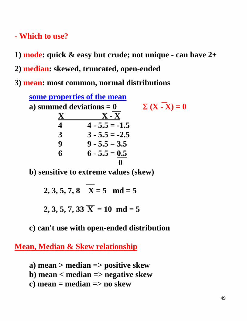
- Which to use?
1) mode: quick & easy but crude; not unique - can have 2+
2) median: skewed, truncated, open-ended
3) mean: most common, normal distributions
some properties of the mean
a) summed deviations = 0 (X - X) = 0
X X - X
4 4 - 5.5 = -1.5
3 3 - 5.5 = -2.5
9 9 - 5.5 = 3.5
6 6 - 5.5 = 0.5
0
b) sensitive to extreme values (skew)
2, 3, 5, 7, 8 X = 5 md = 5
2, 3, 5, 7, 33 X = 10 md = 5
c) can't use with open-ended distribution
Mean, Median & Skew relationship
a) mean > median => positive skew
b) mean < median => negative skew
c) mean = median => no skew
50
CHAPTER 4 HOMEWORK
1 a – c
2
8 a – d
18
51
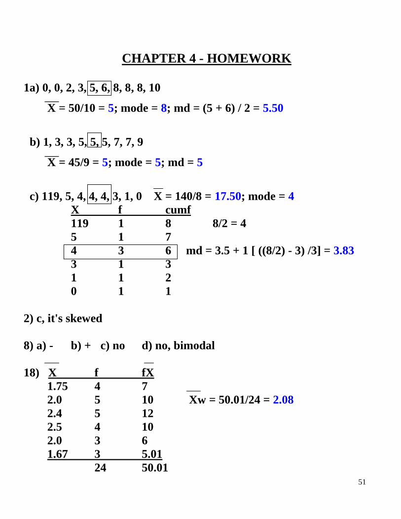
CHAPTER 4 - HOMEWORK
1a) 0, 0, 2, 3, 5, 6, 8, 8, 8, 10
X = 50/10 = 5; mode = 8; md = (5 + 6) / 2 = 5.50
b) 1, 3, 3, 5, 5, 5, 7, 7, 9
X = 45/9 = 5; mode = 5; md = 5
c) 119, 5, 4, 4, 4, 3, 1, 0 X = 140/8 = 17.50; mode = 4
X f cumf
119 1 8 8/2 = 4
5 1 7
4 3 6 md = 3.5 + 1 [ ((8/2) - 3) /3] = 3.83
3 1 3
1 1 2
0 1 1
2) c, it's skewed
8) a) - b) + c) no d) no, bimodal
18) X f fX
1.75 4 7
2.0 5 10 Xw = 50.01/24 = 2.08
2.4 5 12
2.5 4 10
2.0 3 6
1.67 3 5.01
24 50.01
52
- Al calculated the average height of people in a random sample to
figure out how high he should make the pull-down security bars on
a new roller coaster. He says the average height is 5’10” but his boss
says not everyone is 5’10”. He wants to know about what height to
expect – what is the dispersion or spread of heights?
Betty graphs data she collected on frequency of failing grades for
grammar school students as a function of tv shows watched and
finds a very peaked graph shifted to the left. She knows it’s
leptokurtic and skewed but can she attach values to say how
leptokutic and how skewed?
53
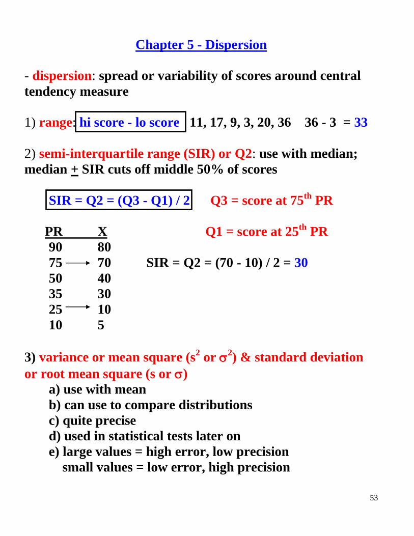
Chapter 5 - Dispersion
- dispersion: spread or variability of scores around central
tendency measure
1) range: hi score - lo score 11, 17, 9, 3, 20, 36 36 - 3 = 33
2) semi-interquartile range (SIR) or Q2: use with median;
median + SIR cuts off middle 50% of scores
SIR = Q2 = (Q3 - Q1) / 2 Q3 = score at 75th
PR
PR X Q1 = score at 25th
PR
90 80
75 70 SIR = Q2 = (70 - 10) / 2 = 30
50 40
35 30
25 10
10 5
3) variance or mean square (s2 or 2
) & standard deviation
or root mean square (s or )
a) use with mean
b) can use to compare distributions
c) quite precise
d) used in statistical tests later on
e) large values = high error, low precision
small values = low error, high precision
54
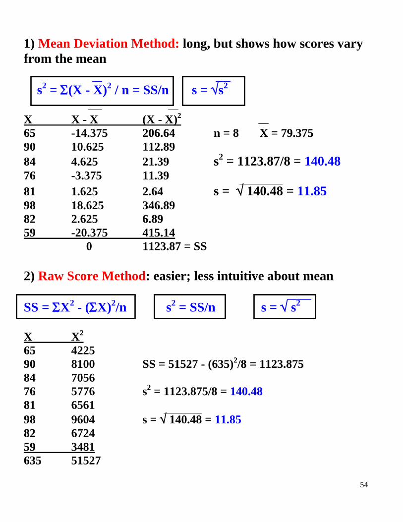
1) Mean Deviation Method: long, but shows how scores vary
from the mean
s2 = (X - X)
2 / n = SS/n s = s
2
X X - X (X - X)
2
65 -14.375 206.64 n = 8 X = 79.375
90 10.625 112.89
84 4.625 21.39 s2 = 1123.87/8 = 140.48
76 -3.375 11.39
81 1.625 2.64 s = 140.48 = 11.85
98 18.625 346.89
82 2.625 6.89
59 -20.375 415.14
0 1123.87 = SS
2) Raw Score Method: easier; less intuitive about mean
SS = X2 - (X)
2/n s
2 = SS/n s = s
2
X X2
65 4225
90 8100 SS = 51527 - (635)2/8 = 1123.875
84 7056
76 5776 s2 = 1123.875/8 = 140.48
81 6561
98 9604 s = 140.48 = 11.85
82 6724
59 3481
635 51527
55
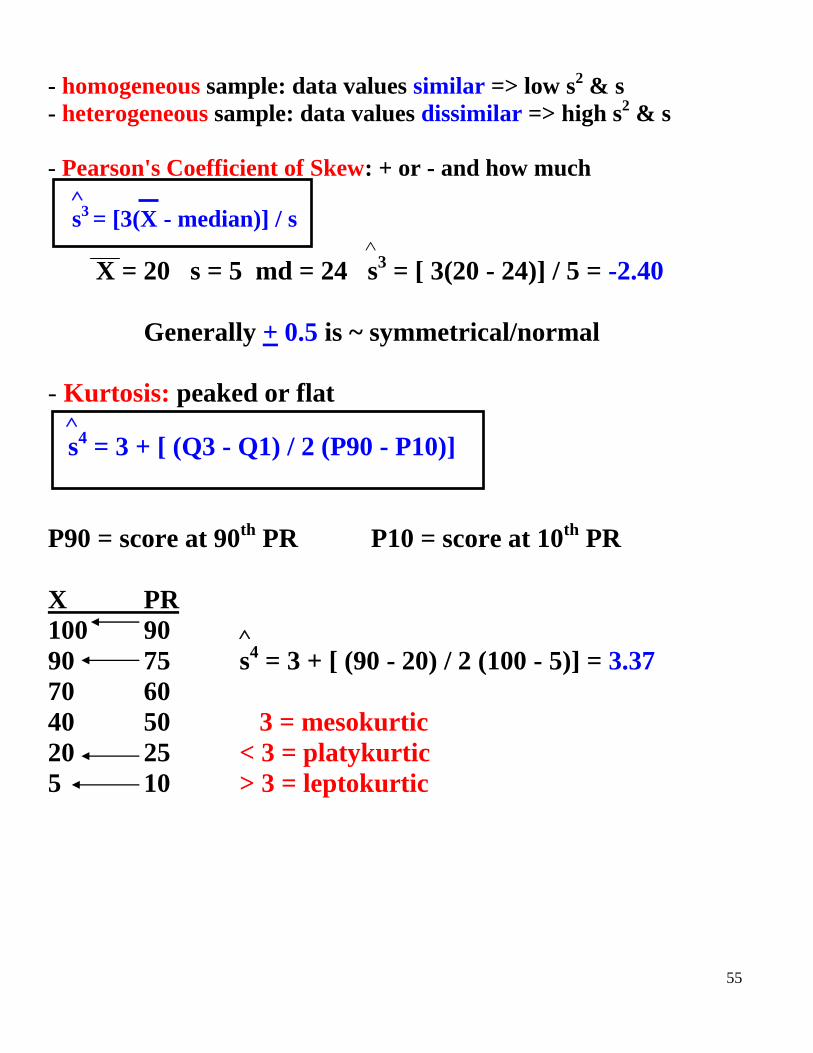
- homogeneous sample: data values similar => low s2 & s
- heterogeneous sample: data values dissimilar => high s2 & s
- Pearson's Coefficient of Skew: + or - and how much
s3 = [3(X - median)] / s
X = 20 s = 5 md = 24 s3 = [ 3(20 - 24)] / 5 = -2.40
Generally + 0.5 is ~ symmetrical/normal
- Kurtosis: peaked or flat s
4 = 3 + [ (Q3 - Q1) / 2 (P90 - P10)]
P90 = score at 90th
PR P10 = score at 10th
PR
X PR
100 90
90 75 s4 = 3 + [ (90 - 20) / 2 (100 - 5)] = 3.37
70 60
40 50 3 = mesokurtic
20 25 < 3 = platykurtic
5 10 > 3 = leptokurtic
56
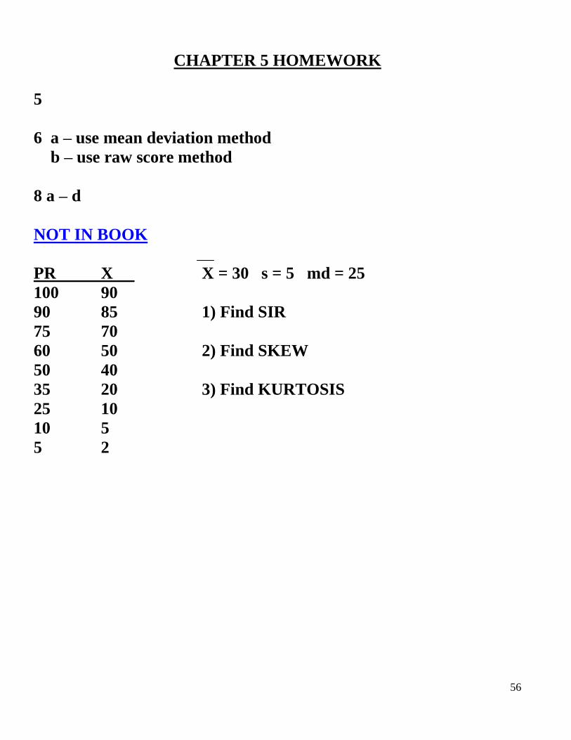
CHAPTER 5 HOMEWORK
5
6 a – use mean deviation method
b – use raw score method
8 a – d
NOT IN BOOK
PR X X = 30 s = 5 md = 25
100 90
90 85 1) Find SIR
75 70
60 50 2) Find SKEW
50 40
35 20 3) Find KURTOSIS
25 10
10 5
5 2
57
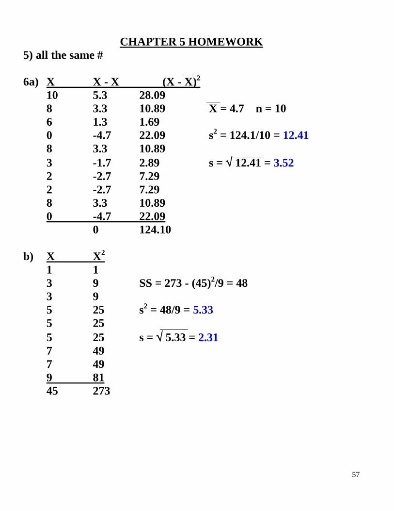
CHAPTER 5 HOMEWORK
5) all the same #
6a) X X - X (X - X)2
10 5.3 28.09
8 3.3 10.89 X = 4.7 n = 10
6 1.3 1.69
0 -4.7 22.09 s2 = 124.1/10 = 12.41
8 3.3 10.89
3 -1.7 2.89 s = 12.41 = 3.52
2 -2.7 7.29
2 -2.7 7.29
8 3.3 10.89
0 -4.7 22.09
0 124.10
b) X X2
1 1
3 9 SS = 273 - (45)2/9 = 48
3 9
5 25 s2 = 48/9 = 5.33
5 25
5 25 s = 5.33 = 2.31
7 49
7 49
9 81
45 273
58
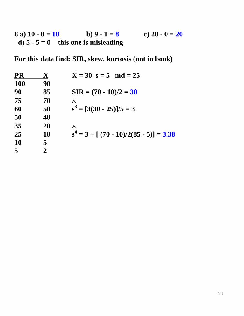
8 a) 10 - 0 = 10 b) 9 - 1 = 8 c) 20 - 0 = 20
d) 5 - 5 = 0 this one is misleading
For this data find: SIR, skew, kurtosis (not in book)
PR X X = 30 s = 5 md = 25
100 90
90 85 SIR = (70 - 10)/2 = 30
75 70
60 50 s3 = [3(30 - 25)]/5 = 3
50 40
35 20
25 10 s4 = 3 + [ (70 - 10)/2(85 - 5)] = 3.38
10 5
5 2

59
- Is there a simpler method to examine percentile ranks and
compare values other than the PR formula?
- Mitch has the mean and standard deviation values for a
quiz that a class just took. He also has his grade on the quiz.
How can he determine how many people did worse than him
and how many did better?
- If you know a country club takes people whose income is in
the top 5% of the city and you know the average income of
the city and standard deviation, can you use your income to
figure out if you can get in the club?
60
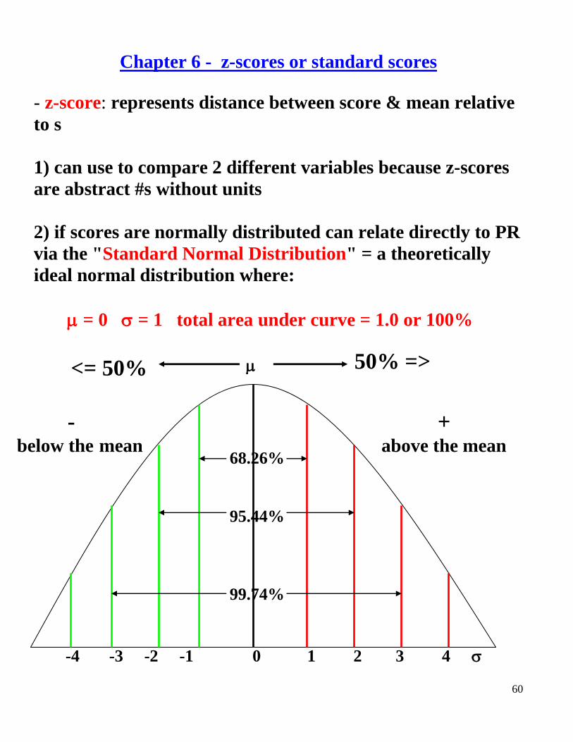
Chapter 6 - z-scores or standard scores
- z-score: represents distance between score & mean relative
to s
1) can use to compare 2 different variables because z-scores
are abstract #s without units
2) if scores are normally distributed can relate directly to PR
via the "Standard Normal Distribution" = a theoretically
ideal normal distribution where:
= 0 = 1 total area under curve = 1.0 or 100%
+ above the mean
- below the mean
50% => <= 50%
-4 -3 -2 -1 0 1 2 3 4
68.26%
95.44%
99.74%

61
3) when you transform data to z-scores
a) mean = 0
b) sum of squared z-scores = n
c) s = 1
z = (X - X)/s z = (X - )/
sample population
e.g., for IQ = 100 = 15; someone got an IQ of 130
z = (130 - 100)/15 = +2.00
so are 2 standard deviations above the mean
e.g., when 2 scores come from different distributions is hard
to compare; z-scores let you do it
psych = 50 = 10
bio = 48 = 4
Bob got a 60 on psych & 56 on bio; for which course should
he expect a better grade?
Psych z = (60 - 50)/10 = +1.00
Bio z = (56 - 48)/4 = +2.00 would expect better grade bio!!!
62
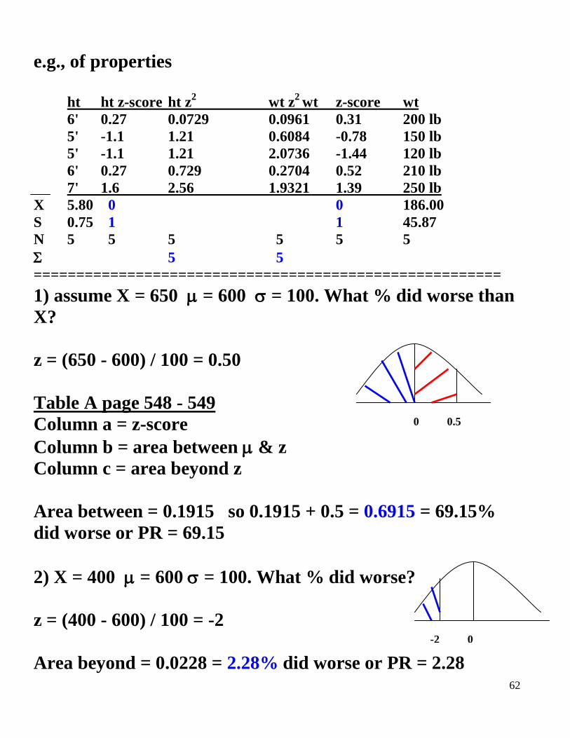
e.g., of properties
ht ht z-score ht z
2 wt z
2 wt z-score wt
6' 0.27 0.0729 0.0961 0.31 200 lb
5' -1.1 1.21 0.6084 -0.78 150 lb
5' -1.1 1.21 2.0736 -1.44 120 lb
6' 0.27 0.729 0.2704 0.52 210 lb
7' 1.6 2.56 1.9321 1.39 250 lb
X 5.80 0 0 186.00
S 0.75 1 1 45.87
N 5 5 5 5 5 5
5 5
=======================================================
1) assume X = 650 = 600 = 100. What % did worse than
X?
z = (650 - 600) / 100 = 0.50
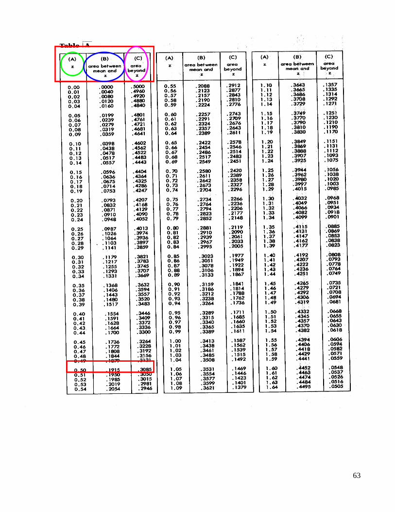
Table A page 548 - 549
Column a = z-score
Column b = area between & z
Column c = area beyond z
Area between = 0.1915 so 0.1915 + 0.5 = 0.6915 = 69.15%
did worse or PR = 69.15
2) X = 400 = 600 = 100. What % did worse?
z = (400 - 600) / 100 = -2
Area beyond = 0.0228 = 2.28% did worse or PR = 2.28
0 0.5
-2 0
63
64

65
3) What % of cases fall between X = 650 and X = 400 if
= 600 = 100?
z = (650 - 600) / 100 = 0.5 z = (400 - 600) / 100 = -2
0.1915 + 0.4772 = 0.6687 = 66.87%
4) What % fall between X = 700 and X = 800 if = 600
= 100?
z = (700 - 600) / 100 = 1 z = (800 - 600) /100 = 2
0.4772 - 0.3413 = 0.1359 = 13.59%
RULE: ++ or -- => subtract column b
+ - => add column b
5) Suppose a golf club takes only top 3% of population in
income where = 500k = 25k. You make 520k. Can you
get in?
column c gives beyond so
find 0.03 in c & get z that goes
with it z = 1.88
so.... 1.88 = (X - 500) / 25 X = 547K
(1.88) (25) = X - 500 so you cannot get in!!!
(1.88) (25) + 500 = X
0 ?
0.5
0 1 2
-2 0 0.5
0.5
0.03 or 3%
66
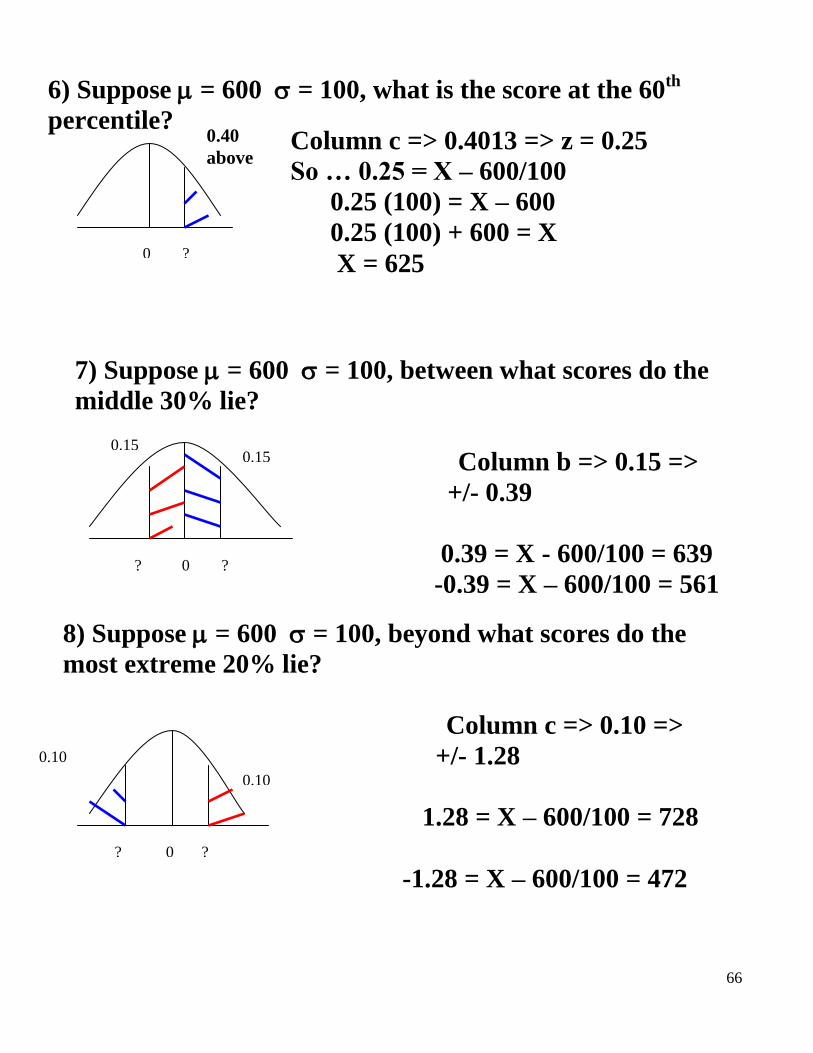
6) Suppose = 600 = 100, what is the score at the 60th
percentile?
7)
0.40
above
0 ?
Column c => 0.4013 => z = 0.25
So … 0.25 = X – 600/100
0.25 (100) = X – 600
0.25 (100) + 600 = X
X = 625
7) Suppose = 600 = 100, between what scores do the
middle 30% lie?
Column b => 0.15 =>
+/- 0.39
0.39 = X - 600/100 = 639
-0.39 = X – 600/100 = 561
0.15 0.15
? 0 ?
8) Suppose = 600 = 100, beyond what scores do the
most extreme 20% lie?
Column c => 0.10 =>
+/- 1.28
1.28 = X – 600/100 = 728
-1.28 = X – 600/100 = 472
0.10
0.10
? 0 ?

67
CHAPTER 6 - HOMEWORK
1 a, c, e
2 a, c, e, g, I
3 a (60 & 25)
b (70 & 45)
c (60 & 70, 45 & 70)
7 a, f, g

68
CHAPTER 6 - HOMEWORK
1a) z = (55 - 45.2) / 10.4 = 0.94
c) z = (45.2 - 45.2) / 10.4 = 0
e) z = (68.4 - 45.2) / 10.4 = 2.23
2a) 0.4798 c) 0.0987 e) 0.4505
g) 0.4901 i) 0.4990
3a) (60 - 50) / 10 = 1
0.3413 x1000 = 341.3 cases
(25 - 50) / 10 = -2.5
0.4938 x 1000 = 493.8 cases
b) (70 - 50) / 10 = 2
0.0228 x 1000 = 22.8 cases
(45 - 50) / 10 = -0.5
0.6915 x 1000 = 691.5 cases
c) (60 - 50) / 10 = 1
(70 - 50) / 10 = 2
0.4772 - 0.3413 = 0.1359 x 1000 = 135.9 cases
(45 - 50) / 10 = -0.5
(70 - 50) / 10 = 2
0.4772 + 0.1915 = 0.6687 x 1000 = 668.7 cases
0 1
-2.5 0
0 2
-0.5 0
0 1 2
-0.5 0 2
69
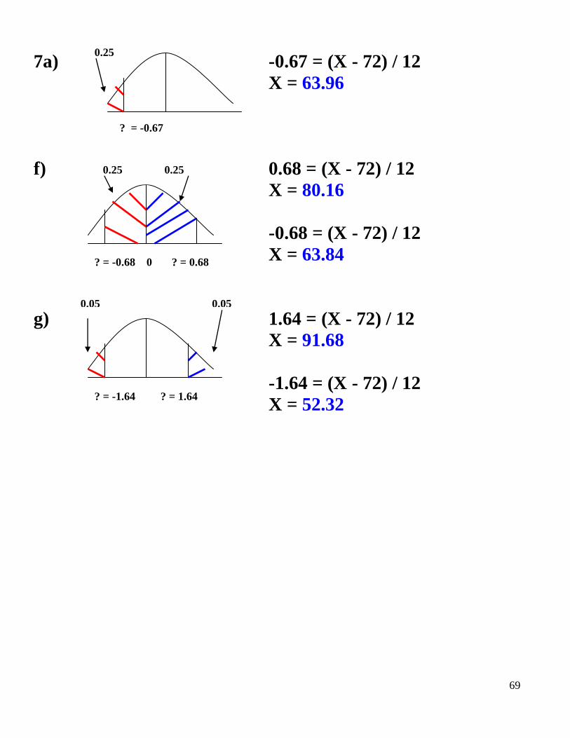
7a) -0.67 = (X - 72) / 12
X = 63.96
f) 0.68 = (X - 72) / 12
X = 80.16
-0.68 = (X - 72) / 12
X = 63.84
g) 1.64 = (X - 72) / 12
X = 91.68
-1.64 = (X - 72) / 12
X = 52.32
0.25
0.25 0.25
? = -0.67
? = -0.68 0 ? = 0.68
0.05 0.05
? = -1.64 ? = 1.64
70
sesty = sy [N ( 1 - r2)] / (N - 2) r = (zxzy) / N
by = (r) (sy/sx) a = Y - byX Y = a + byX
rs = 1 - [ (6D2) / [N (N
2 - 1)]] 1 = r
2 + k
2
zy' = (r)(zx) Y' = Y + (zy')(sy)
Y' = Y + [ (r)(sy/sx)(X - X)]
r = XY - [(X)(Y) / N]
[X2 - [(X)
2 /N]] [Y
2 - [(Y)
2 / N]]
71
- Sue wants to know if there is a relationship between how
well students do on a quiz and how much test anxiety they
report prior to taking it.
- Bill has teachers rank their students by how popular they
think they are and then wants to know if there is a
relationship between the popularity ranks and the students’
GPA.
- Sandy wants to know if there is a relationship between
number of depressed people and SES.

72
Chapter 8 - Correlation
- correlation: relationship between 2 variables
- correlation coefficient: measure used to express extent or
strength of relationship 1) positive correlation: 0 < r < 1; score high on 1 variable &
score high on the other; score low on 1 variable score &
score low on the other; positive slope; 1.0 = perfect
correlation
2) negative correlation: -1 < r < 0; score high on 1 variable &
score low on the other; negative slope; -1.0 = perfect
correlation
positive negative
3) 0 = no correlation, no linear relationship
4) looking for a linear relationship - others exist (e.g., u-
shaped), but correlation only measures linear
5) correlation = causation
6) |r| < 0.29 small correlation, weak relationship
|r| 0.3 - 0.49 medium correlation / relationship
|r| 0.5 - 1.0 large correlation, strong relationship

73
- scatter diagram: graphic means to show data points &
correlation & (later) regression - centroid: X, Y point ( )
1) Pearson r: for interval & ratio data
a) z-score method
r = (zxzy) / N N = # pairs
X Zx Y Zy ZxZy 1 -1.5 4 -1.5 2.25
3 -1 7 -1.0 1
5 -0.5 10 -0.5 0.25 r = 7/7 = 1.00
7 0 13 0 0
9 0.5 16 0.5 0.25
11 1 19 1.0 1
13 1.5 22 1.5 2.25
= 7 Good if already have z-scores, otherwise is a pain!
If already have info: (zxzy) = 4.90 N = 7, then 4.9/7 = 0.70
then it's easy.
0
2
4
6
8
10
12
0 2 4 6 8 10
ht
wt
Ht Wt
2 3
4 7
5 10
9 11
5 7.75 mean
74
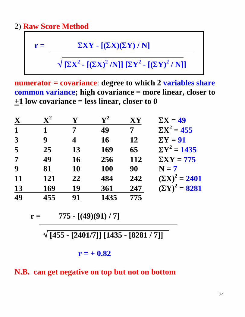
2) Raw Score Method
r = XY - [(X)(Y) / N]
[X2 - [(X)
2 /N]] [Y
2 - [(Y)
2 / N]]
numerator = covariance: degree to which 2 variables share
common variance; high covariance = more linear, closer to
+1 low covariance = less linear, closer to 0
X X2 Y Y
2 XY X = 49
1 1 7 49 7 X2 = 455
3 9 4 16 12 Y = 91
5 25 13 169 65 Y2 = 1435
7 49 16 256 112 XY = 775
9 81 10 100 90 N = 7
11 121 22 484 242 (X)2 = 2401
13 169 19 361 247 (Y)2 = 8281
49 455 91 1435 775
r = 775 - [(49)(91) / 7]
[455 - [2401/7]] [1435 - [8281 / 7]]
r = + 0.82
N.B. can get negative on top but not on bottom
75
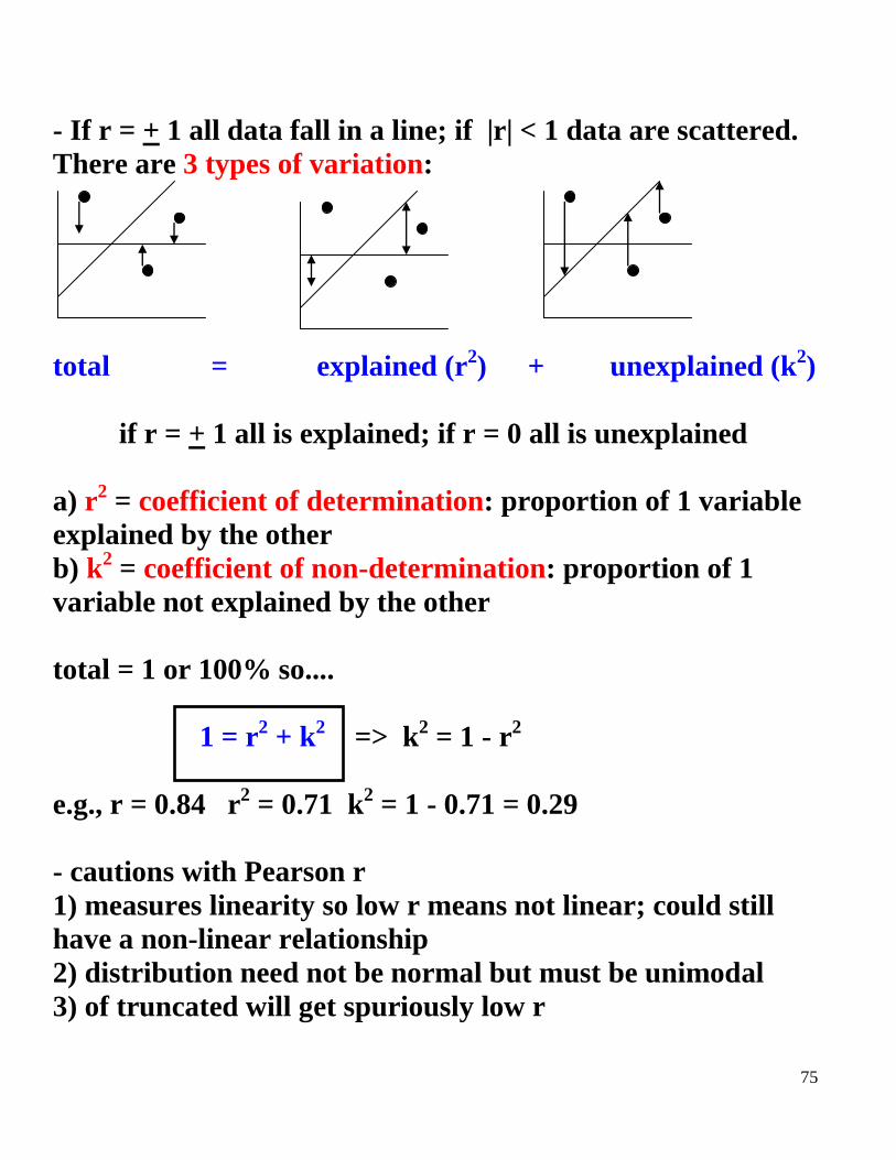
- If r = + 1 all data fall in a line; if |r| < 1 data are scattered.
There are 3 types of variation:
total = explained (r2) + unexplained (k
2)
if r = + 1 all is explained; if r = 0 all is unexplained
a) r2 = coefficient of determination: proportion of 1 variable
explained by the other
b) k2 = coefficient of non-determination: proportion of 1
variable not explained by the other
total = 1 or 100% so....
1 = r2 + k
2 => k
2 = 1 - r
2
e.g., r = 0.84 r2 = 0.71 k
2 = 1 - 0.71 = 0.29
- cautions with Pearson r
1) measures linearity so low r means not linear; could still
have a non-linear relationship
2) distribution need not be normal but must be unimodal
3) of truncated will get spuriously low r

76
2) Spearman r: with ordinal data; rs
a) both variables must be rank ordered
b) non-parametric test: looks at ranks only (parametric
uses actual #s)
rs = 1 - [ (6D2) / [N (N
2 - 1)]]
D = rank X - rank Y D = 0 N = # pairs
X rank X Y rank Y D D
2
140 1 63 6 -5 25
120 5 70 3 2 4
136 2 72 1 1 1
100 6 69 4 2 4
129 3 65 5 -2 4
125 4 71 2 2 4
0 42
rs = 1 - [ (6 42) / [6 ( 36 - 1)]] = - 0.20
- Tied Scores: if tied must take this into account to be fair
X rank X adjusted rank X
140 1 1
120 4 4.5 (4 + 5) / 2 = 4.50
136 2 2
100 6 6 take mean of tied ranks
120 5 4.5 assign mean rank
125 3 3
77
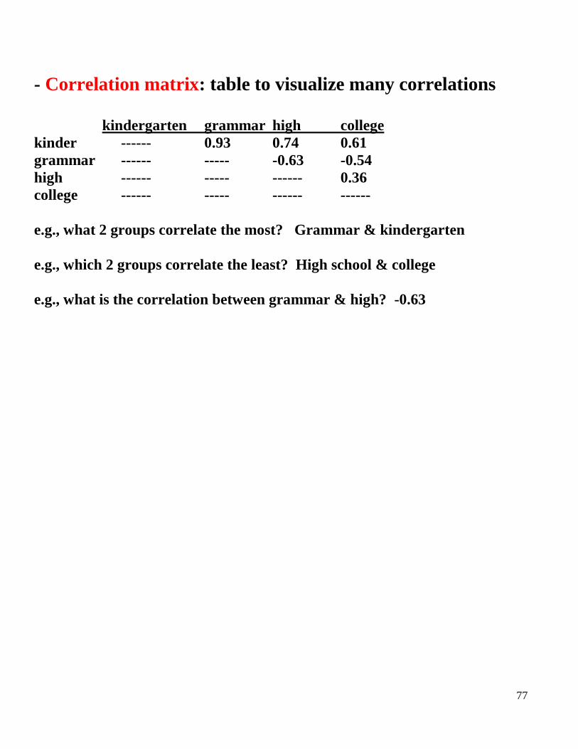
- Correlation matrix: table to visualize many correlations
kindergarten grammar high college
kinder ------ 0.93 0.74 0.61
grammar ------ ----- -0.63 -0.54
high ------ ----- ------ 0.36
college ------ ----- ------ ------
e.g., what 2 groups correlate the most? Grammar & kindergarten
e.g., which 2 groups correlate the least? High school & college
e.g., what is the correlation between grammar & high? -0.63
78
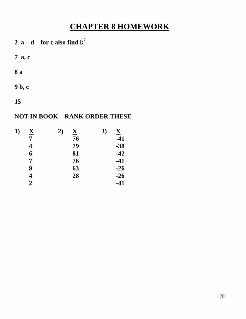
CHAPTER 8 HOMEWORK
2 a – d for c also find k2
7 a, c
8 a
9 b, c
15
NOT IN BOOK – RANK ORDER THESE
1) X 2) X 3) X
7 76 -41
4 79 -38
6 81 -42
7 76 -41
9 63 -26
4 28 -26
2 -41
79
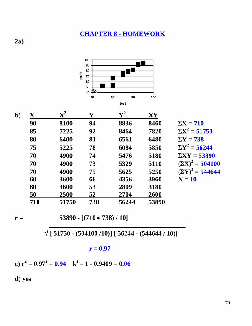
CHAPTER 8 - HOMEWORK
2a)
b) X X2 Y Y
2 XY
90 8100 94 8836 8460 X = 710
85 7225 92 8464 7820 X2 = 51750
80 6400 81 6561 6480 Y = 738
75 5225 78 6084 5850 Y2 = 56244
70 4900 74 5476 5180 XY = 53890
70 4900 73 5329 5110 (X)2 = 504100
70 4900 75 5625 5250 (Y)2 = 544644
60 3600 66 4356 3960 N = 10
60 3600 53 2809 3180
50 2500 52 2704 2600
710 51750 738 56244 53890
r = 53890 - [(710 738) / 10]
[ 51750 - (504100 /10)] [ 56244 - (544644 / 10)]
r = 0.97
c) r2 = 0.97
2 = 0.94 k
2 = 1 - 0.9409 = 0.06
d) yes
40
50
60
70
80
90
100
40 60 80 100
test
gra
de
80
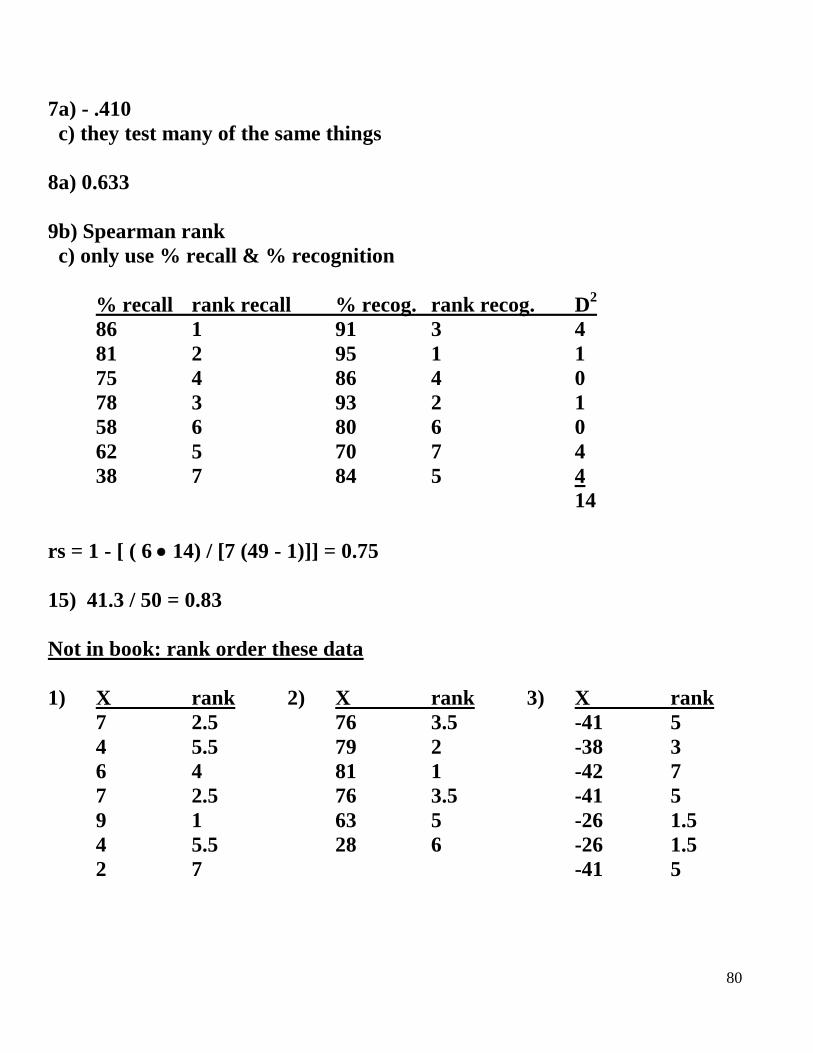
7a) - .410
c) they test many of the same things
8a) 0.633
9b) Spearman rank
c) only use % recall & % recognition
% recall rank recall % recog. rank recog. D2
86 1 91 3 4
81 2 95 1 1
75 4 86 4 0
78 3 93 2 1
58 6 80 6 0
62 5 70 7 4
38 7 84 5 4
14
rs = 1 - [ ( 6 14) / [7 (49 - 1)]] = 0.75
15) 41.3 / 50 = 0.83
Not in book: rank order these data
1) X rank 2) X rank 3) X rank
7 2.5 76 3.5 -41 5
4 5.5 79 2 -38 3
6 4 81 1 -42 7
7 2.5 76 3.5 -41 5
9 1 63 5 -26 1.5
4 5.5 28 6 -26 1.5
2 7 -41 5

81
- Joe has a set of data correlating number of books read per month with age.
He wants to plot these data on a graph and draw a line to show the general
linear trend of the data.
- Carol has a set of data on height as a function of how many grams of
protein children had on average per day. She then wants to predict the
height of an individual assuming they had 10 grams of protein on average
per day.
82
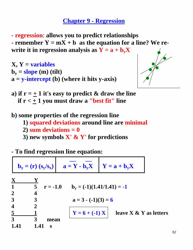
Chapter 9 - Regression
- regression: allows you to predict relationships
- remember Y = mX + b as the equation for a line? We re-
write it in regression analysis as Y = a + byX
X, Y = variables
by = slope (m) (tilt)
a = y-intercept (b) (where it hits y-axis)
a) if r = + 1 it's easy to predict & draw the line
if r < + 1 you must draw a "best fit" line
b) some properties of the regression line
1) squared deviations around line are minimal
2) sum deviations = 0
3) new symbols X' & Y' for predictions
- To find regression line equation:
by = (r) (sy/sx) a = Y - byX Y = a + byX
X Y
1 5 r = -1.0 by = (-1)(1.41/1.41) = -1
2 4
3 3 a = 3 - (-1)(3) = 6
4 2
5 1 Y = 6 + (-1) X leave X & Y as letters
3 3 mean
1.41 1.41 s
83
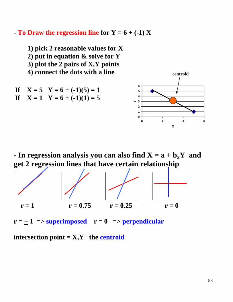
- To Draw the regression line for Y = 6 + (-1) X
1) pick 2 reasonable values for X
2) put in equation & solve for Y
3) plot the 2 pairs of X,Y points
4) connect the dots with a line
- In regression analysis you can also find X = a + bxY and
get 2 regression lines that have certain relationship
r = 1 r = 0.75 r = 0.25 r = 0
r = + 1 => superimposed r = 0 => perpendicular
intersection point = X,Y the centroid
0
1
2
3
4
5
6
0 2 4 6
X
Y
If X = 5 Y = 6 + (-1)(5) = 1
If X = 1 Y = 6 + (-1)(1) = 5
centroid

84
- To predict Y if know X
Y' = Y + [ (r)(sy/sx)(X - X)]
Given: X = 70 sx = 4 Y = 75 sy = 8 r = 0.6 If Sue got a 62 on X
what did she get on Y?
Y' = 75 + [ (0.6) (8/4) (62 - 70) ] = 65.40
- If you have z-scores
zy' = (r)(zx) Y' = Y + (zy')(sy)
Given: X = 62 X = 70 sx = 4 zx = -2 Y = 75 sy = 8 r = 0.6
a) zy' = (0.6) (-2) = -1.20
b) Y' = 75 + (-1.2)(8) = 65.40
85
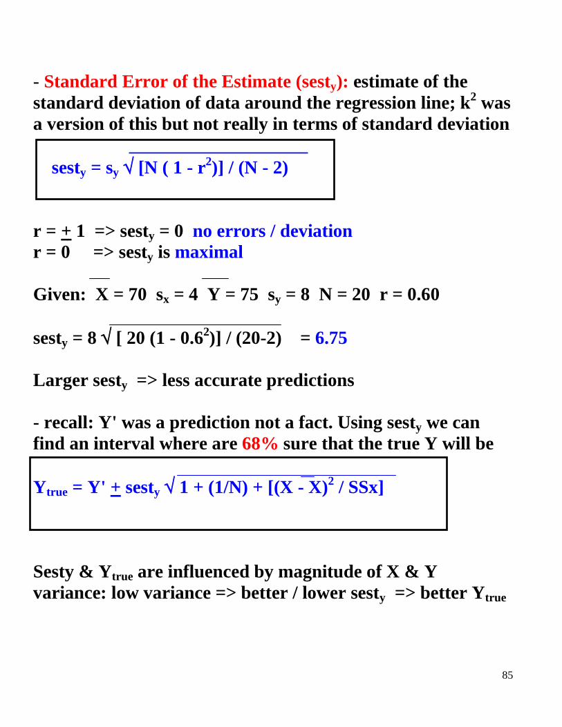
- Standard Error of the Estimate (sesty): estimate of the
standard deviation of data around the regression line; k2 was
a version of this but not really in terms of standard deviation
sesty = sy [N ( 1 - r2)] / (N - 2)
r = + 1 => sesty = 0 no errors / deviation
r = 0 => sesty is maximal
Given: X = 70 sx = 4 Y = 75 sy = 8 N = 20 r = 0.60
sesty = 8 [ 20 (1 - 0.62)] / (20-2) = 6.75
Larger sesty => less accurate predictions
- recall: Y' was a prediction not a fact. Using sesty we can
find an interval where are 68% sure that the true Y will be
Ytrue = Y' + sesty 1 + (1/N) + [(X - X)2 / SSx]
Sesty & Ytrue are influenced by magnitude of X & Y
variance: low variance => better / lower sesty => better Ytrue

86
- Homoscedasticity: where variance of 1 variable is constant
at all levels of the other variable
- Heteroscedasticity: where variance of 1 variable is not
constant at all levels of the other variable
Homoscedasticity Heteroscedasticity
- Post-Hoc Fallacy: assuming a cause & effect relationship
from correlation data
87
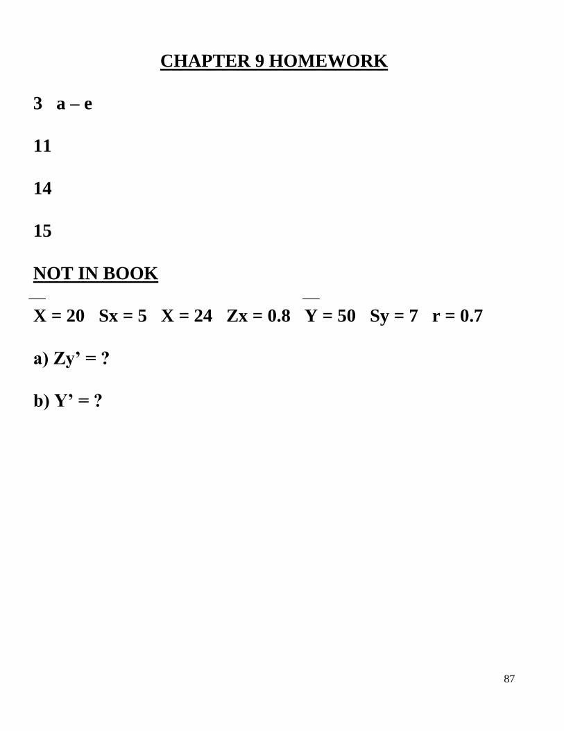
CHAPTER 9 HOMEWORK
3 a – e
11
14
15
NOT IN BOOK
X = 20 Sx = 5 X = 24 Zx = 0.8 Y = 50 Sy = 7 r = 0.7
a) Zy’ = ?
b) Y’ = ?

88
CHAPTER 9 - HOMEWORK
3a) by = (0.36)(0.5 / 12) = 0.02 a = 2.85 - (0.015)(49) = 2.12
Y = 2.12 + 0.02 X
b) Y = 2.12 + (0.02)(1) = 2.14 Y = 2.12 + (0.02) (3) = 2.18
c) Y' = 2.85 + (0.36)(0.5 / 12)(65 - 49) = 3.09
d) sesty = 0.5 [60(1 - 0.362)] / (60 - 2) = 0.47
e) r2 = 0.36
2 = 0.13 k
2 = 1 – 0.13 = 0.87
11) no = post hoc fallacy
14) no, could be curvilinear or some other relationship
15) 0.20 => yes, will probably do different
0.90 => no, will do about the same
Given: X = 20 sx = 5 X = 24 zx = 0.8 Y = 50 sy = 7 r = 0.7
a) zy' = (0.7)(0.8) = 0.56
b) Y' = 50 + (0.56)(7) = 53.92
0
1
2
3
0 1 2 3 4
x
y
89
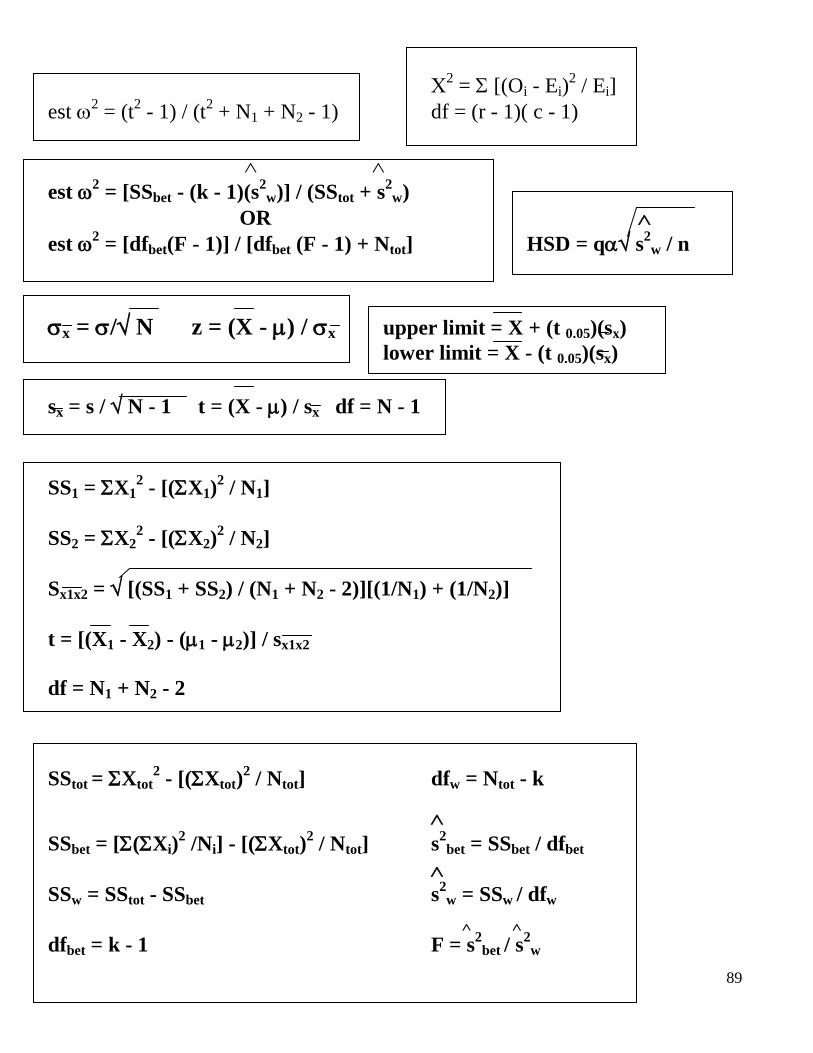
2 = [(Oi - Ei)
2 / Ei]
est 2 = (t
2 - 1) / (t
2 + N1 + N2 - 1) df = (r - 1)( c - 1)
est 2 = [SSbet - (k - 1)(s
2w)] / (SStot + s
2w)
OR
est 2 = [dfbet(F - 1)] / [dfbet (F - 1) + Ntot] HSD = q s
2w / n
x = / N z = (X - ) / x upper limit = X + (t 0.05)(sx)
lower limit = X - (t 0.05)(sx)
sx = s / N - 1 t = (X - ) / sx df = N - 1
SS1 = X12 - [(X1)
2 / N1]
SS2 = X22 - [(X2)
2 / N2]
Sx1x2 = [(SS1 + SS2) / (N1 + N2 - 2)][(1/N1) + (1/N2)]
t = [(X1 - X2) - (1 - 2)] / sx1x2
df = N1 + N2 - 2
SStot = Xtot2 - [(Xtot)
2 / Ntot] dfw = Ntot - k
SSbet = [(Xi)2 /Ni] - [(Xtot)
2 / Ntot] s
2bet = SSbet / dfbet
SSw = SStot - SSbet s2w = SSw / dfw
dfbet = k - 1 F = s2bet / s
2w

90
- Are there any underlying concepts that guide our choice of
statistical tests?
- Are there standards that we can compare our results to in
order to see if there are statistically significant differences?
- Are we always right or are there errors we should be aware
of?
91
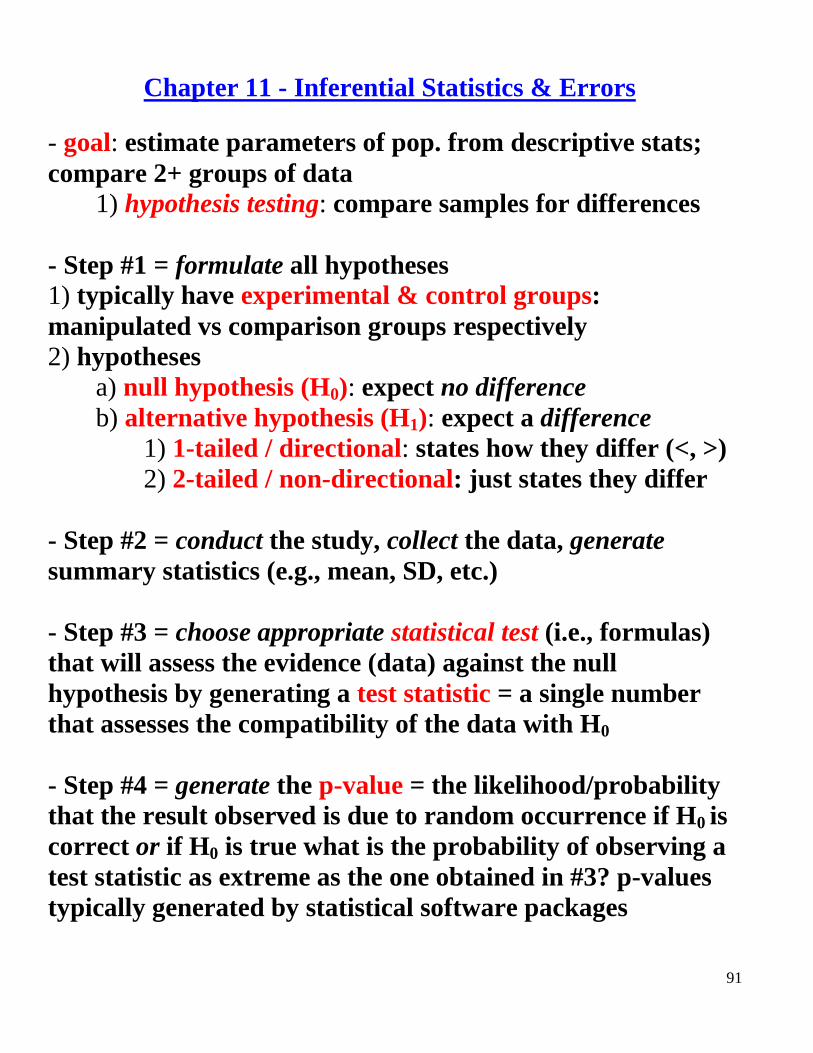
Chapter 11 - Inferential Statistics & Errors
- goal: estimate parameters of pop. from descriptive stats;
compare 2+ groups of data 1) hypothesis testing: compare samples for differences
- Step #1 = formulate all hypotheses
1) typically have experimental & control groups:
manipulated vs comparison groups respectively
2) hypotheses
a) null hypothesis (H0): expect no difference
b) alternative hypothesis (H1): expect a difference
1) 1-tailed / directional: states how they differ (<, >)
2) 2-tailed / non-directional: just states they differ
- Step #2 = conduct the study, collect the data, generate
summary statistics (e.g., mean, SD, etc.)
- Step #3 = choose appropriate statistical test (i.e., formulas)
that will assess the evidence (data) against the null
hypothesis by generating a test statistic = a single number
that assesses the compatibility of the data with H0
- Step #4 = generate the p-value = the likelihood/probability
that the result observed is due to random occurrence if H0 is
correct or if H0 is true what is the probability of observing a
test statistic as extreme as the one obtained in #3? p-values
typically generated by statistical software packages

92
- Step #5a (using software) = compare p-value to a fixed
significance level () that the scientific community agrees
that there is statistical significance (most common = 0.05 &
0.01): Rule: p < => reject H0 p > => accept H0
= 0.05 p = 0.03 reject H0, are different
= 0.01 p = 0.06 accept H0, no different
- Step #5b (by hand) =
a) each statistical test is associated with a theoretical
distribution of values (sampling distribution) of what would
happen (theoretically) if every sample of a particular size
were studied (i.e., what test statistic would you expect for a
given sample size)
b) when you generate a test statistic (using a formula)
you can then go to a table with the sampling distribution and
for a given -level & sample size find what test statistic value
would expect if H0 is true – if your test statistic > table value
reject H0 = there is a statistically significant difference
- Central Limit Theorum (CLT): method to construct a
sampling distribution of the population mean, providing a
way to test H0; assumes that if random samples of fixed N
from any pop. are drawn & X calculated then:
1) distribution of means becomes normal
2) grand mean approaches mean of pop.
3) standard deviation decreases
93
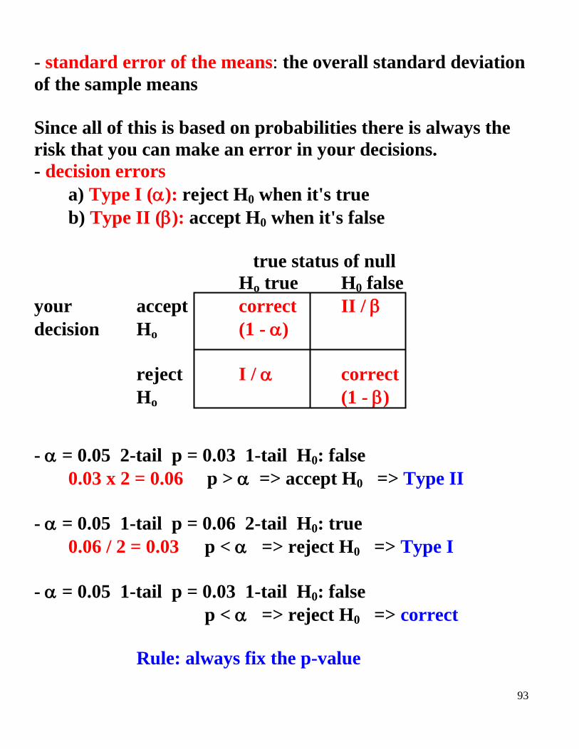
- standard error of the means: the overall standard deviation
of the sample means
Since all of this is based on probabilities there is always the
risk that you can make an error in your decisions.
- decision errors
a) Type I (): reject H0 when it's true
b) Type II (): accept H0 when it's false
true status of null
Ho true H0 false
your accept correct II /
decision Ho (1 - )
reject I / correct
Ho (1 - )
- = 0.05 2-tail p = 0.03 1-tail H0: false
0.03 x 2 = 0.06 p > => accept H0 => Type II
- = 0.05 1-tail p = 0.06 2-tail H0: true
0.06 / 2 = 0.03 p < => reject H0 => Type I
- = 0.05 1-tail p = 0.03 1-tail H0: false
p < => reject H0 => correct
Rule: always fix the p-value

94
CHAPTER 11 - HOMEWORK
7
14
15
21
22-26

95
CHAPTER 11 - HOMEWORK
7) approaches normal, mean approaches mean, s decreases
14) no
15) yes; 1-tail => <,> 2-tail => just differ
21) 0.05
p H0
22) p < => reject => Type I 0.01 0.008 T
23) p > => accept => correct 0.05 0.08 T
24) p > => accept => Type II 0.05 0.06 F
25) p < => reject => correct 0.05 0.03 F
26) p < => reject => correct 0.01 0.005 F
96
- John has access to all the records for inductees into the US Army
since it began and knows the average IQ and standard deviation for
this population. He has a group of new inductees and wants to know
if their average IQ differs significantly from past years.
- Kelly knows that sampling errors always exist so the sample mean
will not exactly match the true population mean. Can she determine
a range of values that will cover the true mean with some degree of
confidence?
97
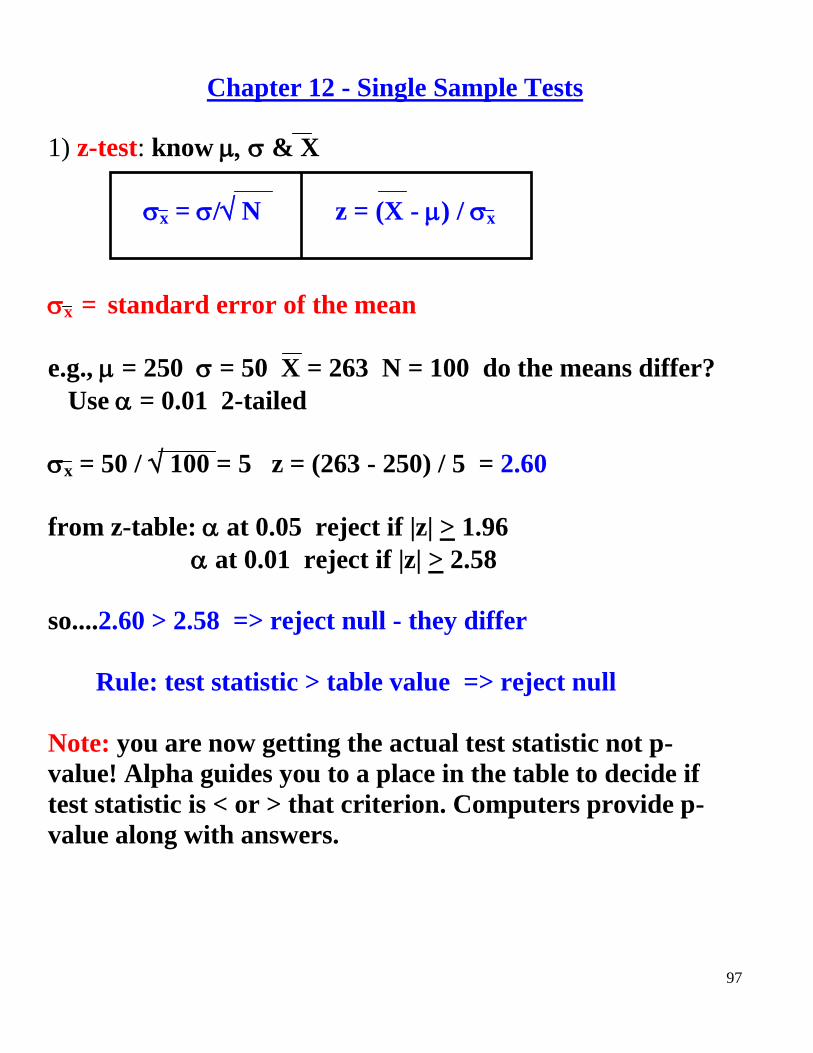
Chapter 12 - Single Sample Tests
1) z-test: know & X
x = / N z = (X - ) / x
x = standard error of the mean
e.g., = 250 = 50 X = 263 N = 100 do the means differ?
Use = 0.01 2-tailed
x = 50 / 100 = 5 z = (263 - 250) / 5 = 2.60
from z-table: at 0.05 reject if |z| > 1.96
at 0.01 reject if |z| > 2.58
so....2.60 > 2.58 => reject null - they differ
Rule: test statistic > table value => reject null
Note: you are now getting the actual test statistic not p-
value! Alpha guides you to a place in the table to decide if
test statistic is < or > that criterion. Computers provide p-
value along with answers.
98
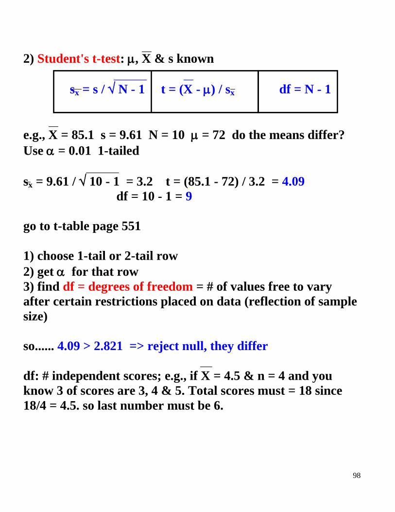
2) Student's t-test: , X & s known
sx = s / N - 1 t = (X - ) / sx df = N - 1
e.g., X = 85.1 s = 9.61 N = 10 = 72 do the means differ?
Use = 0.01 1-tailed
sx = 9.61 / 10 - 1 = 3.2 t = (85.1 - 72) / 3.2 = 4.09
df = 10 - 1 = 9
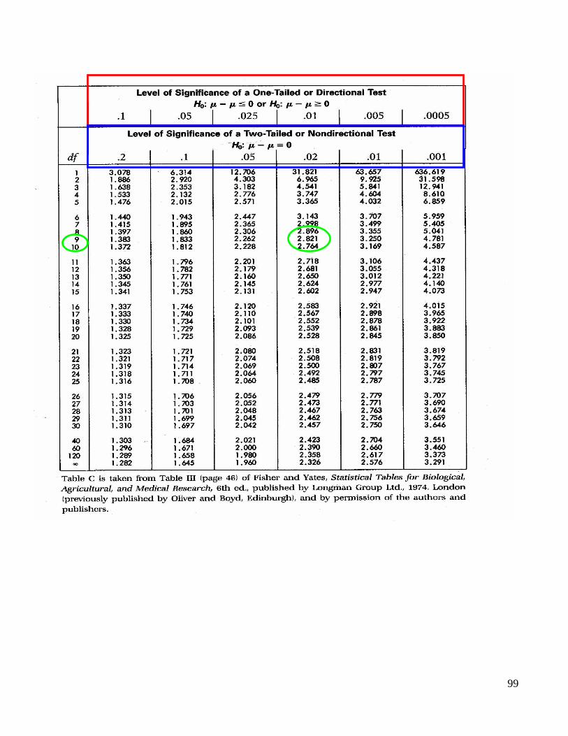
go to t-table page 551
1) choose 1-tail or 2-tail row
2) get for that row
3) find df = degrees of freedom = # of values free to vary
after certain restrictions placed on data (reflection of sample
size)
so...... 4.09 > 2.821 => reject null, they differ
df: # independent scores; e.g., if X = 4.5 & n = 4 and you
know 3 of scores are 3, 4 & 5. Total scores must = 18 since
18/4 = 4.5. so last number must be 6.
99
100
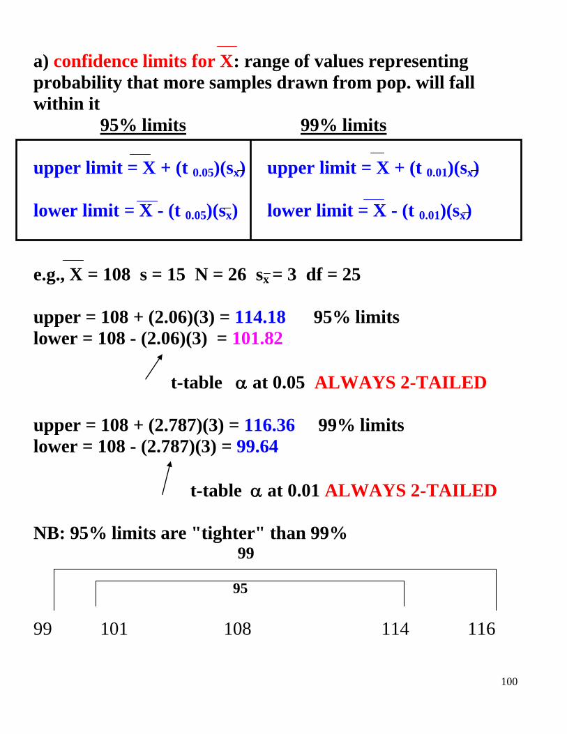
a) confidence limits for X: range of values representing
probability that more samples drawn from pop. will fall
within it
95% limits 99% limits
upper limit = X + (t 0.05)(sx) upper limit = X + (t 0.01)(sx)
lower limit = X - (t 0.05)(sx) lower limit = X - (t 0.01)(sx)
e.g., X = 108 s = 15 N = 26 sx = 3 df = 25
upper = 108 + (2.06)(3) = 114.18 95% limits
lower = 108 - (2.06)(3) = 101.82
t-table at 0.05 ALWAYS 2-TAILED
upper = 108 + (2.787)(3) = 116.36 99% limits
lower = 108 - (2.787)(3) = 99.64
t-table at 0.01 ALWAYS 2-TAILED
NB: 95% limits are "tighter" than 99% 99
95
99 101 108 114 116
101
CHAPTER 12 – HOMEWORK
14
15
29
30
102
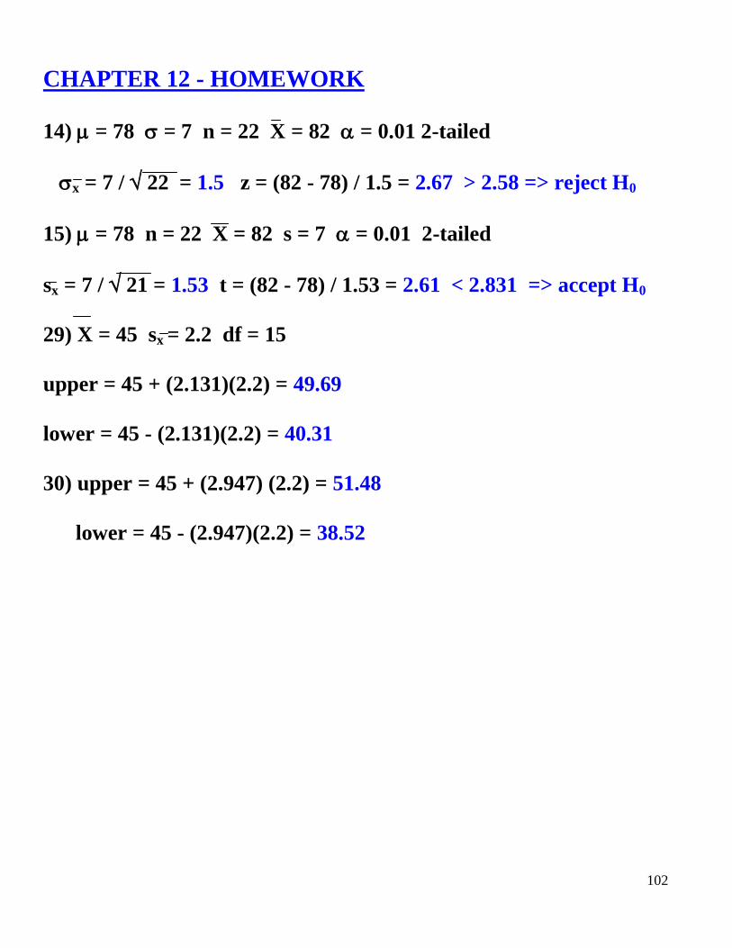
CHAPTER 12 - HOMEWORK
14) = 78 = 7 n = 22 X = 82 = 0.01 2-tailed
x = 7 / 22 = 1.5 z = (82 - 78) / 1.5 = 2.67 > 2.58 => reject H0
15) = 78 n = 22 X = 82 s = 7 = 0.01 2-tailed
sx = 7 / 21 = 1.53 t = (82 - 78) / 1.53 = 2.61 < 2.831 => accept H0
29) X = 45 sx = 2.2 df = 15
upper = 45 + (2.131)(2.2) = 49.69
lower = 45 - (2.131)(2.2) = 40.31
30) upper = 45 + (2.947) (2.2) = 51.48
lower = 45 - (2.947)(2.2) = 38.52

103
- Andy has two groups of rats and wants to see if what he feeds
them affects how fast they run through a maze. One group gets
mashed protein bars to eat and the other gets mashed bananas. He
runs them through the maze and times them. The protein group
runs it in 6.5 seconds on average and the banana group runs it in
10.3 seconds. Is there a significant difference?
- Is there a way to estimate the degree to which the IV really
contributes to the effect seen on the DV?

104
Chapter 13 - 2-Sample Tests
- Student's t-test for unknown population
SS1 = X12 - [(X1)
2 / N1]
SS2 = X22 - [(X2)
2 / N2]
Sx1x2 = [(SS1 + SS2) / (N1 + N2 - 2)][(1/N1) + (1/N2)]
t = [(X1 - X2) - (1 - 2)] / sx1x2 ** 1 - 2 = 0 **
df = N1 + N2 - 2
e.g., X1 = 477 X2 = 11 = 0.05
X12 = 29845 X2
2 = 101 1-tail
X1 = 59.63 X2 = 5.5
N1 = 8 N2 = 2
SS1 = 29845 - [(4772)/8] = 1403.88
SS2 = 101 - [(112)/2] = 40.50
Sx1x2 = [(1403.88 + 40.50) / (8 + 2 - 2)] [ (1/8) + (1/2)] = 10.62
t = (59.63 - 5.50) / 10.62 = 5.10 > 1.86 => reject H0
df = 8 + 2 - 2 = 8

105
- est 2 (omega-squared): many things contribute to p-level
and whether you accept of reject the null; one is 2 or
degree to which IV accounts for variance in DV - how much
are the 2 variables related?
est 2 = (t2 - 1) / (t
2 + N1 + N2 - 1)
- interpret like r2 - higher 2
means have significant findings
e.g., t = 5.097 in previous problem
est 2 = (5.097
2 - 1) / (5.097
2 + 8 + 2 - 1) = 0.714
IV accounts for 71.4% of variance in DV - fairly significant
Can follow this with the confidence limits

106
CHAPTER 13 HOMEWORK
4 also find 2
107
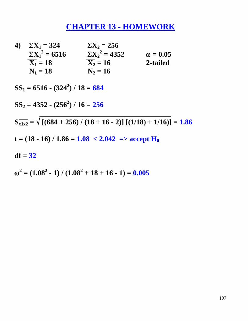
CHAPTER 13 - HOMEWORK
4) X1 = 324 X2 = 256
X12 = 6516 X2
2 = 4352 = 0.05
X1 = 18 X2 = 16 2-tailed
N1 = 18 N2 = 16
SS1 = 6516 - (3242) / 18 = 684
SS2 = 4352 - (2562) / 16 = 256
Sx1x2 = [(684 + 256) / (18 + 16 - 2)] [(1/18) + 1/16)] = 1.86
t = (18 - 16) / 1.86 = 1.08 < 2.042 => accept H0
df = 32
2 = (1.08
2 - 1) / (1.08
2 + 18 + 16 - 1) = 0.005

108
- June has a new drug to control the number of manic episodes
patients experience each month, but she is not sure of the most
effective dose. She gets 30 manic patients and divides them
randomly into 3 groups. She gives one group a low dose, one group
a medium dose and one group a high dose of the drug. She then
monitors them for one month, recording the number of manic
episodes they experience. Group 1 has an average of 6 episodes,
group 2 has 3, and group 3 has 5. Do they differ significantly in
their effect on the number of manic episodes?
- Exactly which doses differ from each other?
109
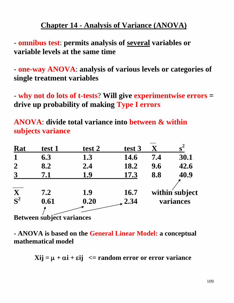
Chapter 14 - Analysis of Variance (ANOVA)
- omnibus test: permits analysis of several variables or
variable levels at the same time
- one-way ANOVA: analysis of various levels or categories of
single treatment variables
- why not do lots of t-tests? Will give experimentwise errors =
drive up probability of making Type I errors
ANOVA: divide total variance into between & within
subjects variance
Rat test 1 test 2 test 3 X s2
1 6.3 1.3 14.6 7.4 30.1
2 8.2 2.4 18.2 9.6 42.6
3 7.1 1.9 17.3 8.8 40.9
X 7.2 1.9 16.7 within subject
S2 0.61 0.20 2.34 variances
Between subject variances
- ANOVA is based on the General Linear Model: a conceptual
mathematical model
Xij = + i + ij <= random error or error variance

110
e.g., blood pressure study: do the 3 means differ? = 0.05
active (X1) passive (X2) relaxed (X3) totals
X 1407 1303 1308 4018
X2 99723 85479 86254 271456
X 70.35 65.15 65.40 --------
N 20 20 20 60
Step 1: add across all rows to get totals; then do equations
1) SStot = Xtot2 - [(Xtot)
2 / Ntot]
271456 - [(40182) / 60] = 2383.94
2) SSbet = [(Xi)2 /Ni] - [(Xtot)
2 / Ntot] i = individual
14072 + 1303
2 + 1308
2 - 4018
2
20 20 20 60 = 344.04
3) SSw = SStot - SSbet
2383.94 - 344.04 = 2039.90
4) dfbet = k - 1 k = # conditions
3 - 1 = 2
5) dfw = Ntot - k
60 - 3 = 57
111
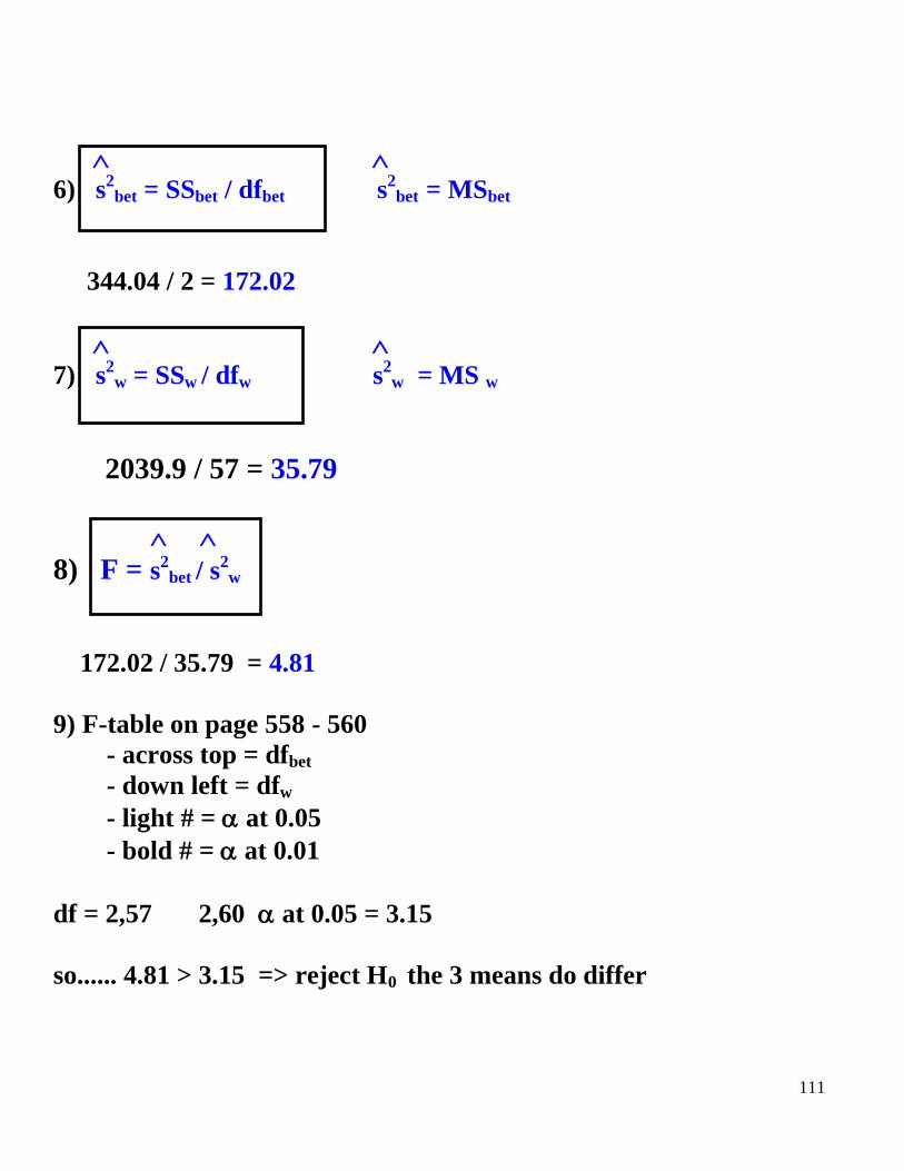
6) s2
bet = SSbet / dfbet s2bet = MSbet
344.04 / 2 = 172.02
7) s2
w = SSw / dfw s2w = MS w
2039.9 / 57 = 35.79
8) F = s2bet / s
2w
172.02 / 35.79 = 4.81
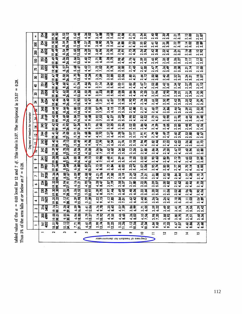
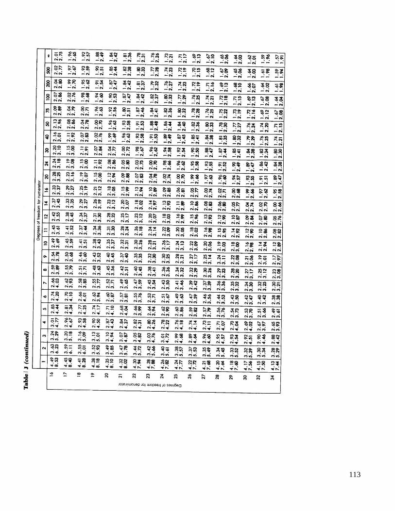
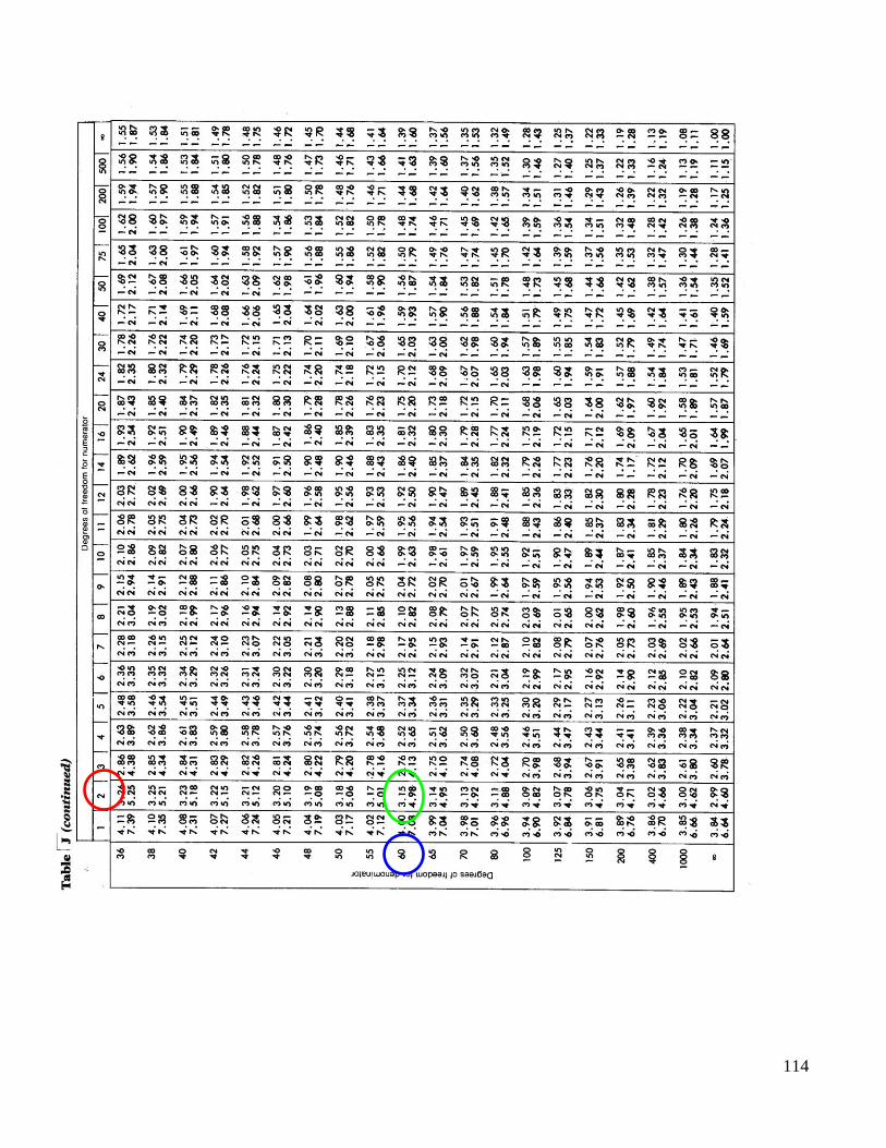
9) F-table on page 558 - 560
- across top = dfbet
- down left = dfw
- light # = at 0.05
- bold # = at 0.01
df = 2,57 2,60 at 0.05 = 3.15
so...... 4.81 > 3.15 => reject H0 the 3 means do differ
112
113
114
115
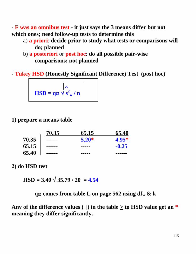
- F was an omnibus test - it just says the 3 means differ but not
which ones; need follow-up tests to determine this a) a priori: decide prior to study what tests or comparisons will
do; planned b) a posteriori or post hoc: do all possible pair-wise
comparisons; not planned
- Tukey HSD (Honestly Significant Difference) Test (post hoc)
HSD = q s2w / n
1) prepare a means table
70.35 65.15 65.40
70.35 ------ 5.20* 4.95*
65.15 ------ ----- -0.25
65.40 ------ ----- ------
2) do HSD test
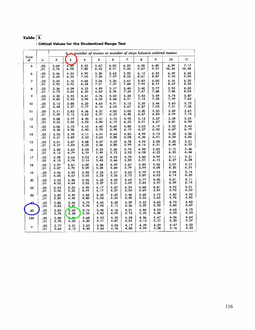
HSD = 3.40 35.79 / 20 = 4.54
q comes from table L on page 562 using dfw & k
Any of the difference values (| |) in the table > to HSD value get an *
meaning they differ significantly.
116
117
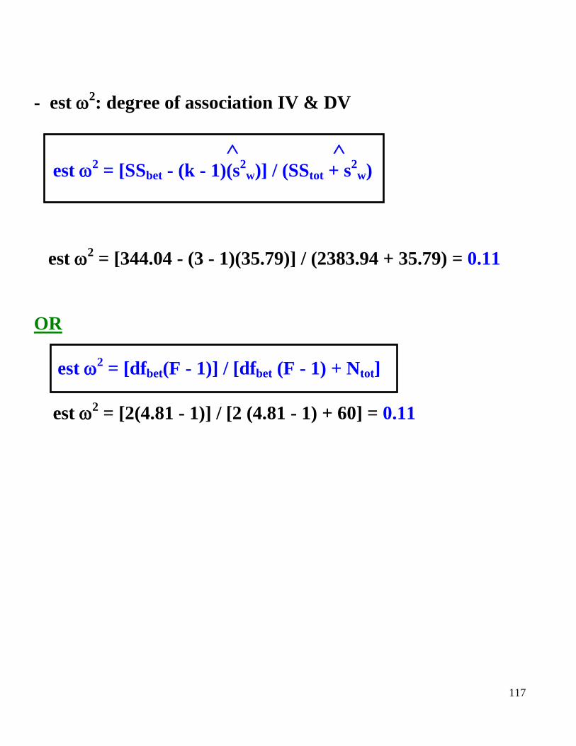
- est 2: degree of association IV & DV
est 2 = [SSbet - (k - 1)(s
2w)] / (SStot + s
2w)
est 2 = [344.04 - (3 - 1)(35.79)] / (2383.94 + 35.79) = 0.11
OR
est 2 = [dfbet(F - 1)] / [dfbet (F - 1) + Ntot]
est 2 = [2(4.81 - 1)] / [2 (4.81 - 1) + 60] = 0.11

118
CHAPTER 14 HOMEWORK
7 d, e, f, h
119
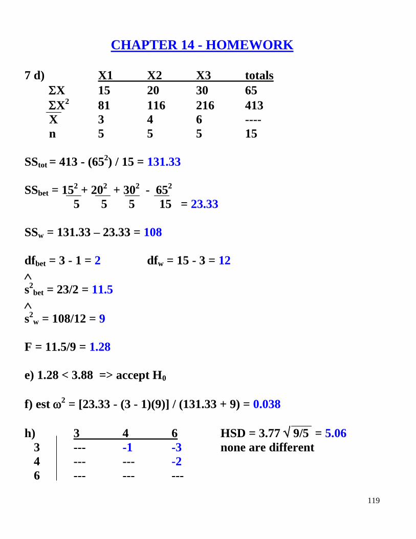
CHAPTER 14 - HOMEWORK
7 d) X1 X2 X3 totals
X 15 20 30 65
X2 81 116 216 413
X 3 4 6 ----
n 5 5 5 15
SStot = 413 - (652) / 15 = 131.33
SSbet = 152 + 20
2 + 30
2 - 65
2
5 5 5 15 = 23.33
SSw = 131.33 – 23.33 = 108
dfbet = 3 - 1 = 2 dfw = 15 - 3 = 12
s2
bet = 23/2 = 11.5
s2
w = 108/12 = 9
F = 11.5/9 = 1.28
e) 1.28 < 3.88 => accept H0
f) est 2 = [23.33 - (3 - 1)(9)] / (131.33 + 9) = 0.038
h) 3 4 6 HSD = 3.77 9/5 = 5.06
3 --- -1 -3 none are different
4 --- --- -2
6 --- --- ---
120
- Ed polls a random sample of people by phone to see how much
they agree with the statement that the president is doing a good job:
very good, good, neutral, poor, very poor. Is there a difference in
the frequency with which people give responses for the different
categories?
- Kathy wants to know if people will help someone more or less as a
function of gender of the person needing help. She has Bob & Ann
pretend to drop a bag of groceries on a busy street and records how
many times people stop to help either one of them. Was there a
significant difference in helping versus non-helping for Bob vs
Ann?

121
Chapter 17 - Chi-Squared Test (2)
- nonparametric: does not require normality
- 2: typically with frequencies or proportions from nominal data
1) one-variable X2 or "goodness of fit"
2 = [(Oi - Ei)
2 / Ei] O = observed data
E = expected data
i = individual
strong strong
agree agree undecided disagree disagree
7 12 13 13 10
expected = total answers / # categories = 55/5 = 11
X2 = (7 - 11)
2 + (12 - 11)
2 + (13 - 11)
2 + (13 - 11)
2 + (10 - 11)
2
11 11 11 11 11 = 2.3
df = N - 1 (n = # categories) df = 5 - 1 = 4
X2 table on page 572 at 0.05 => 9.488
2.3 < 9.488 => accept H0 no difference

122

123
2) multi-variable X2: same formula but different way to get
expected
get better get worse
drug a 1 b 17 18
placebo c 9 d 12 21
10 29 39
1) label boxes a - d
2) find expected values
a) (18/39) (10) = 4.6
b) (18/39) (29) = 13.4 x
c) (21/39) (10) = 5.4
d) (21/39) (29) = 15.6
3) use X2 formula
a b c d
(1 - 4.6)
2 + (17 - 13.4)
2 + (9 - 5.4)
2 + (12 - 15.6)
2
4.6 13.4 5.4 15.6 = 7.09
df = (r - 1)(c - 1) r = # rows c = # columns
df = (2 - 1)(2 - 1) = 1 7.09 > 6.635 => reject H0 they differ
fe = fcfr/n

124
CHAPTER 17 – HOMEWORK
5
8

125
CHAPTER 17 - HOMEWORK
5) 4 5 6 7 use = 0.05
11 15 13 29 68/4 = 17
(11 - 17)2 + (15 - 17)
2 + (13 - 17)
2 + (29 - 17)
2
17 17 17 17 = 11.78
df = 4 - 1 = 3 11.78 > 7.815 => reject H0
8) A B
H a 75 b 45 120 use = 0.05
NH c 40 d 80 120
115 125 240
a) (120/240)(115) = 57.5
b) (120/240)(125) = 62.5
c) (120/240)(115) = 57.5
d) (120/240)(125) = 62.5
(75 - 57.5)2 + (45 - 62.5)
2 + (40 - 57.5)
2 + (80 - 62.5)
2
57.5 62.5 57.5 62.5 = 20.4
df = (2 - 1)(2 - 1) = 1
20.4 > 3.841 => reject H0 they differ
126
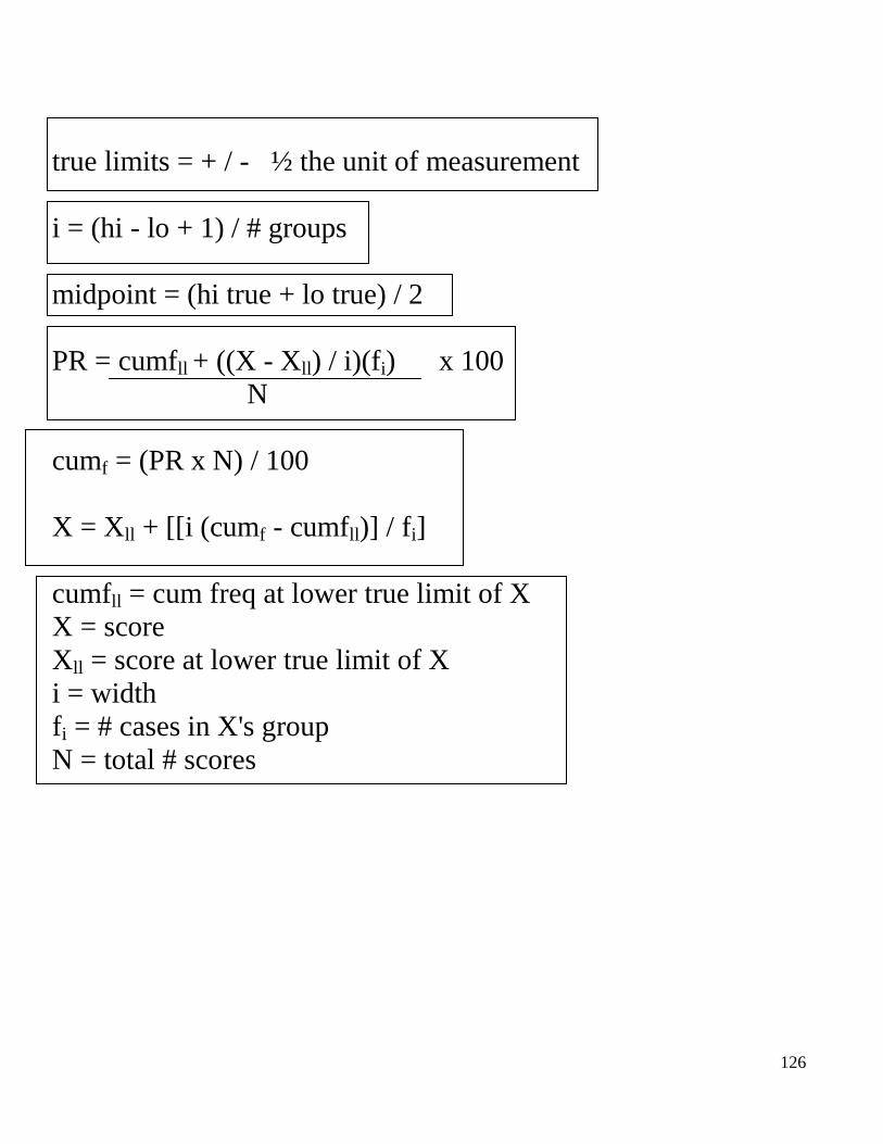
true limits = + / - ½ the unit of measurement
i = (hi - lo + 1) / # groups
midpoint = (hi true + lo true) / 2
PR = cumfll + ((X - Xll) / i)(fi) x 100
N
cumf = (PR x N) / 100
X = Xll + [[i (cumf - cumfll)] / fi]
cumfll = cum freq at lower true limit of X
X = score
Xll = score at lower true limit of X
i = width
fi = # cases in X's group
N = total # scores
127
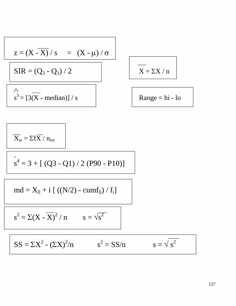
z = (X - X) / s = (X - ) /
SIR = (Q3 - Q1) / 2 X = X / n
s3 = [3(X - median)] / s Range = hi - lo
Xw = fX / ntot
s4 = 3 + [ (Q3 - Q1) / 2 (P90 - P10)]
md = Xll + i [ ((N/2) - cumfll) / fi]
s2 = (X - X)2 / n s = s2
SS = X2 - (X)2/n s2 = SS/n s = s2
128
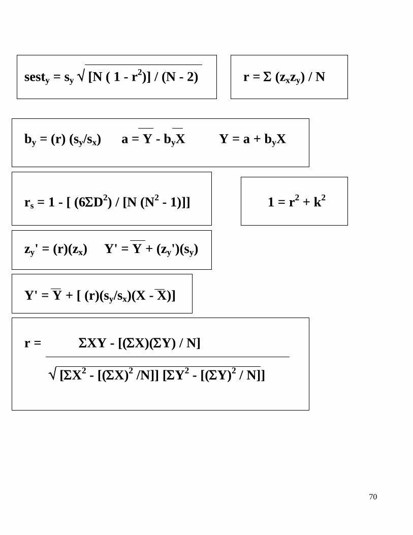
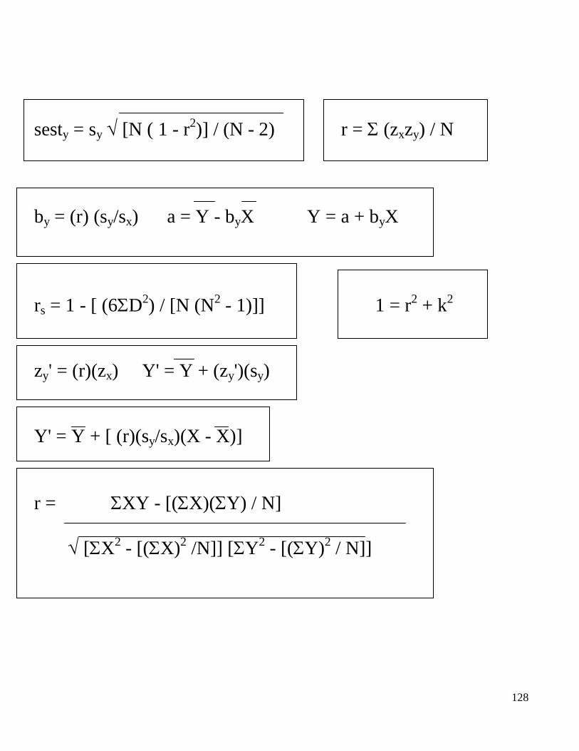
sesty = sy [N ( 1 - r2)] / (N - 2) r = (zxzy) / N
by = (r) (sy/sx) a = Y - byX Y = a + byX
rs = 1 - [ (6D2) / [N (N2 - 1)]] 1 = r2 + k2
zy' = (r)(zx) Y' = Y + (zy')(sy)
Y' = Y + [ (r)(sy/sx)(X - X)]
r = XY - [(X)(Y) / N]
[X2 - [(X)2 /N]] [Y2 - [(Y)2 / N]]
129
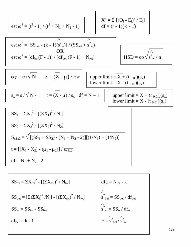
2 = [(Oi - Ei)
2 / Ei]
est 2 = (t
2 - 1) / (t
2 + N1 + N2 - 1) df = (r - 1)( c - 1)
est 2 = [SSbet - (k - 1)(s
2w)] / (SStot + s
2w)
OR
est 2 = [dfbet(F - 1)] / [dfbet (F - 1) + Ntot] HSD = q s
2w / n
x = / N z = (X - ) / x upper limit = X + (t 0.05)(sx)
lower limit = X - (t 0.05)(sx) sx = s / N - 1 t = (X - ) / sx df = N – 1 upper limit = X + (t 0.01)(sx)
lower limit = X - (t 0.01)(sx)
SS1 = X1
2 - [(X1)
2 / N1]
SS2 = X22 - [(X2)
2 / N2]
Sx1x2 = [(SS1 + SS2) / (N1 + N2 - 2)][(1/N1) + (1/N2)]
t = [(X1 - X2) - (1 - 2)] / sx1x2
df = N1 + N2 - 2
SStot = Xtot2 - [(Xtot)
2 / Ntot] dfw = Ntot - k
SSbet = [(Xi)2 /Ni] - [(Xtot)
2 / Ntot] s
2bet = SSbet / dfbet
SSw = SStot - SSbet s
2w = SSw / dfw
dfbet = k - 1 F = s2
bet / s2w
130
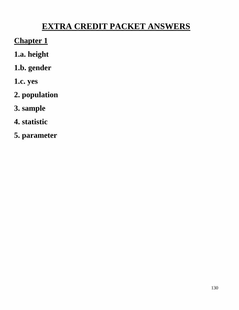
EXTRA CREDIT PACKET ANSWERS
Chapter 1
1.a. height
1.b. gender
1.c. yes
2. population
3. sample
4. statistic
5. parameter
131
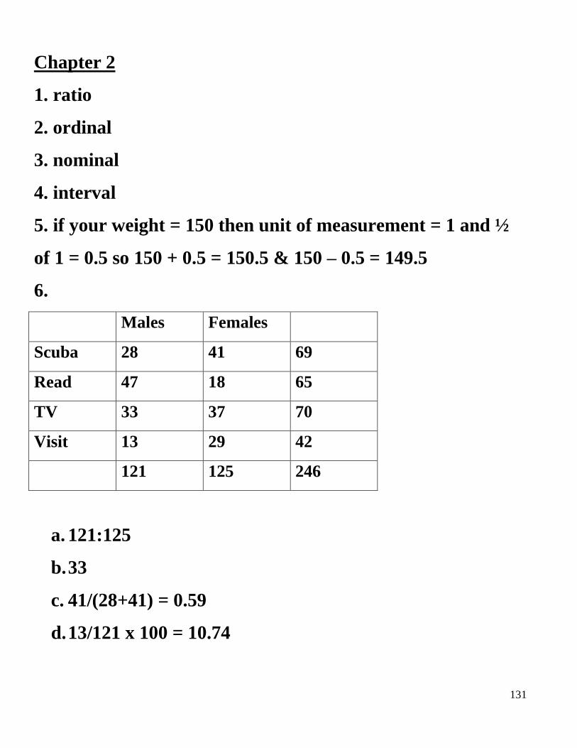
Chapter 2
1. ratio
2. ordinal
3. nominal
4. interval
5. if your weight = 150 then unit of measurement = 1 and ½
of 1 = 0.5 so 150 + 0.5 = 150.5 & 150 – 0.5 = 149.5
6.
Males Females
Scuba 28 41 69
Read 47 18 65
TV 33 37 70
Visit 13 29 42
121 125 246
a. 121:125
b. 33
c. 41/(28+41) = 0.59
d. 13/121 x 100 = 10.74
132
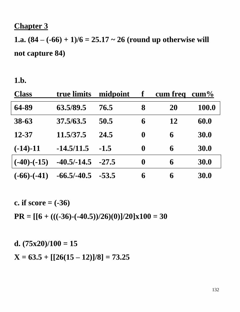
Chapter 3
1.a. (84 – (-66) + 1)/6 = 25.17 ~ 26 (round up otherwise will
not capture 84)
1.b.
Class true limits midpoint f cum freq cum%
64-89 63.5/89.5 76.5 8 20 100.0
38-63 37.5/63.5 50.5 6 12 60.0
12-37 11.5/37.5 24.5 0 6 30.0
(-14)-11 -14.5/11.5 -1.5 0 6 30.0
(-40)-(-15) -40.5/-14.5 -27.5 0 6 30.0
(-66)-(-41) -66.5/-40.5 -53.5 6 6 30.0
c. if score = (-36)
PR = [[6 + (((-36)-(-40.5))/26)(0)]/20]x100 = 30
d. (75x20)/100 = 15
X = 63.5 + [[26(15 – 12)]/8] = 73.25
133
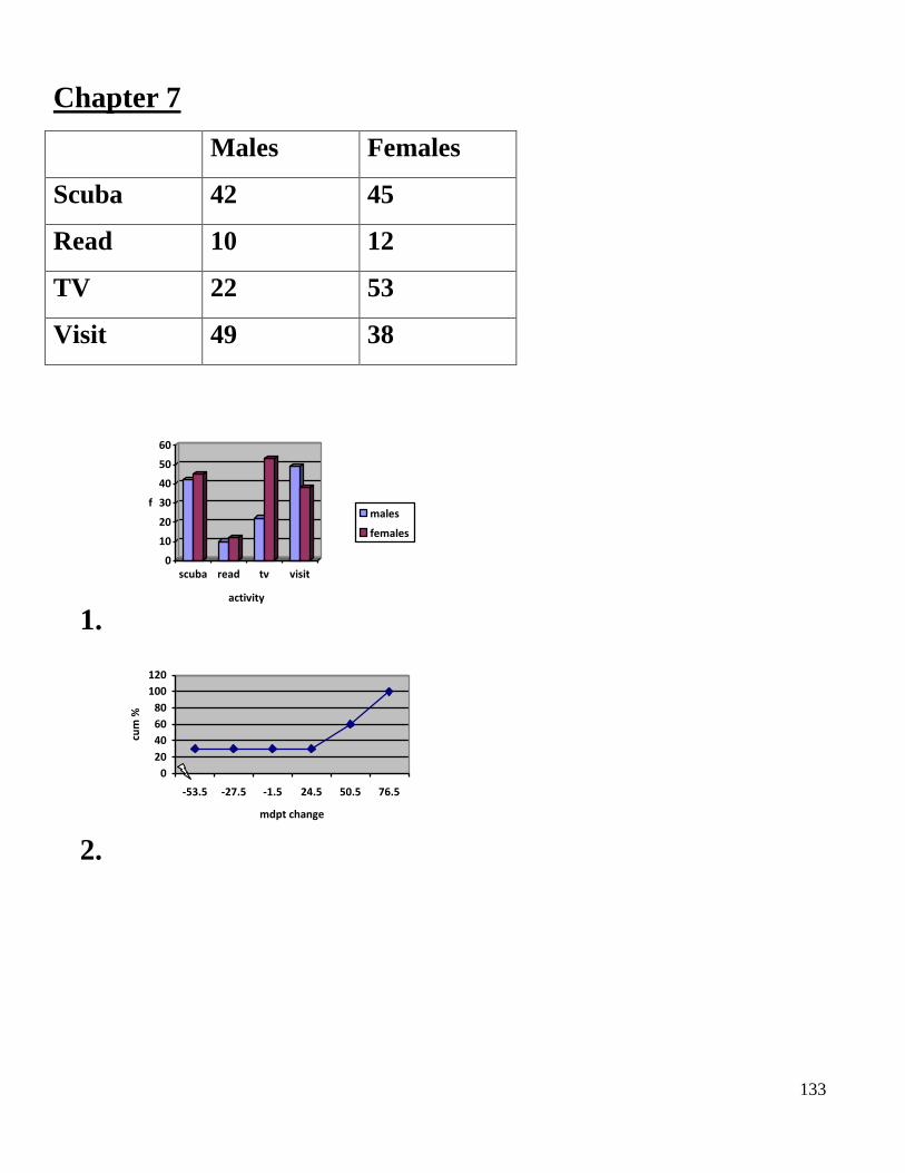
Chapter 7
Males Females
Scuba 42 45
Read 10 12
TV 22 53
Visit 49 38
1.
0
10
20
30
40
50
60
f
scuba read tv visit
activity
males
females
2.
0
20
40
60
80
100
120
-53.5 -27.5 -1.5 24.5 50.5 76.5
mdpt change
cum
%
134
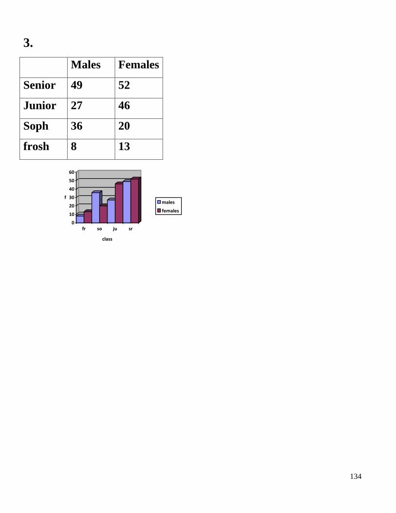
3.
Males Females
Senior 49 52
Junior 27 46
Soph 36 20
frosh 8 13
0
10
20
30
40
50
60
f
fr so ju sr
class
males
females
135
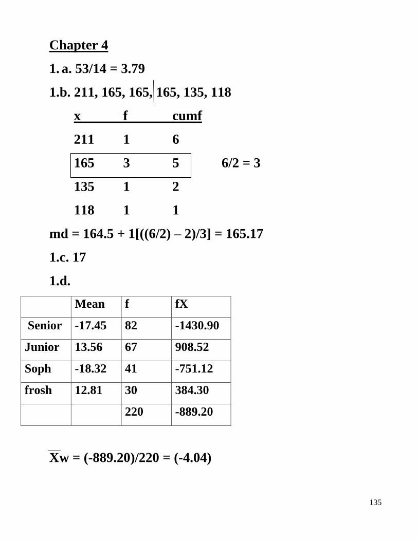
Chapter 4
1. a. 53/14 = 3.79
1.b. 211, 165, 165, 165, 135, 118
x f cumf
211 1 6
165 3 5 6/2 = 3
135 1 2
118 1 1
md = 164.5 + 1[((6/2) – 2)/3] = 165.17
1.c. 17
1.d.
Mean f fX
Senior -17.45 82 -1430.90
Junior 13.56 67 908.52
Soph -18.32 41 -751.12
frosh 12.81 30 384.30
220 -889.20
Xw = (-889.20)/220 = (-4.04)
136
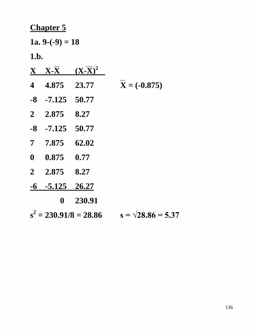
Chapter 5
1a. 9-(-9) = 18
1.b.
X X-X (X-X)2
4 4.875 23.77 X = (-0.875)
-8 -7.125 50.77
2 2.875 8.27
-8 -7.125 50.77
7 7.875 62.02
0 0.875 0.77
2 2.875 8.27
-6 -5.125 26.27
0 230.91
s2 = 230.91/8 = 28.86 s = √28.86 = 5.37
137
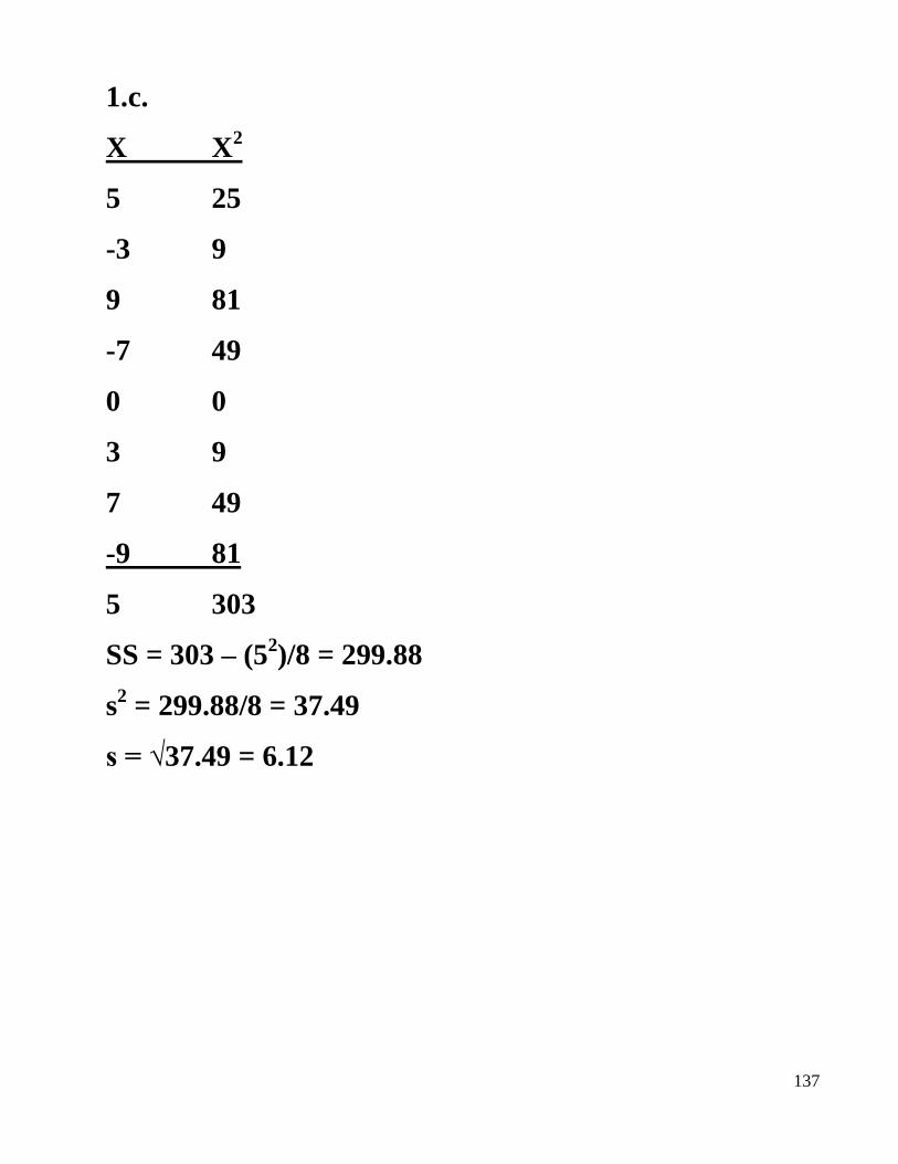
1.c.
X X2
5 25
-3 9
9 81
-7 49
0 0
3 9
7 49
-9 81
5 303
SS = 303 – (52)/8 = 299.88
s2 = 299.88/8 = 37.49
s = √37.49 = 6.12
138
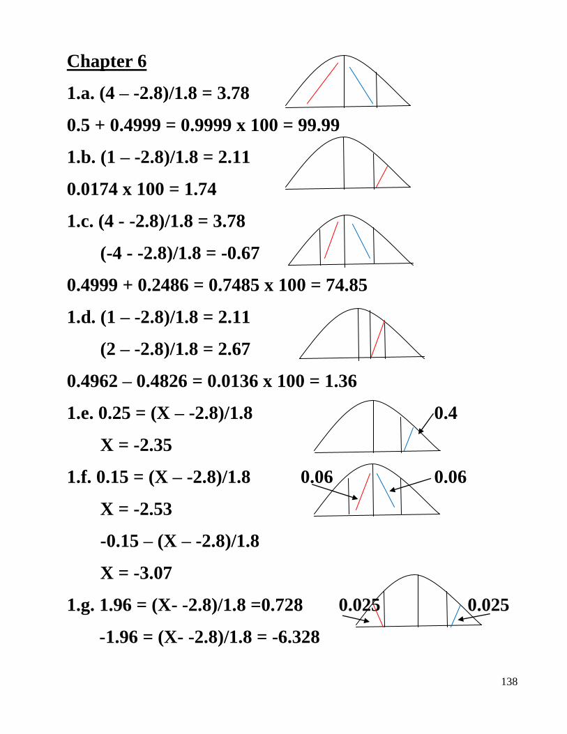
Chapter 6
1.a. (4 – -2.8)/1.8 = 3.78
0.5 + 0.4999 = 0.9999 x 100 = 99.99
1.b. (1 – -2.8)/1.8 = 2.11
0.0174 x 100 = 1.74
1.c. (4 - -2.8)/1.8 = 3.78
(-4 - -2.8)/1.8 = -0.67
0.4999 + 0.2486 = 0.7485 x 100 = 74.85
1.d. (1 – -2.8)/1.8 = 2.11
(2 – -2.8)/1.8 = 2.67
0.4962 – 0.4826 = 0.0136 x 100 = 1.36
1.e. 0.25 = (X – -2.8)/1.8 0.4
X = -2.35
1.f. 0.15 = (X – -2.8)/1.8 0.06 0.06
X = -2.53
-0.15 – (X – -2.8)/1.8
X = -3.07
1.g. 1.96 = (X- -2.8)/1.8 =0.728 0.025 0.025
-1.96 = (X- -2.8)/1.8 = -6.328
139
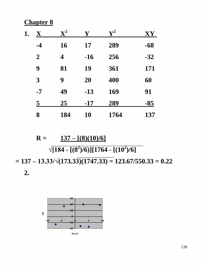
Chapter 8
1. X X2 Y Y
2 XY
-4 16 17 289 -68
2 4 -16 256 -32
9 81 19 361 171
3 9 20 400 60
-7 49 -13 169 91
5 25 -17 289 -85
8 184 10 1764 137
R = 137 – [(8)(10)/6]
√[184 - [(82)/6)][1764 - [(10
2)/6]
= 137 – 13.33/√(173.33)(1747.33) = 123.67/550.33 = 0.22
2.
-20
-10
0
10
20
30
-10 -5 0 5 10
hrs tv
wt
140
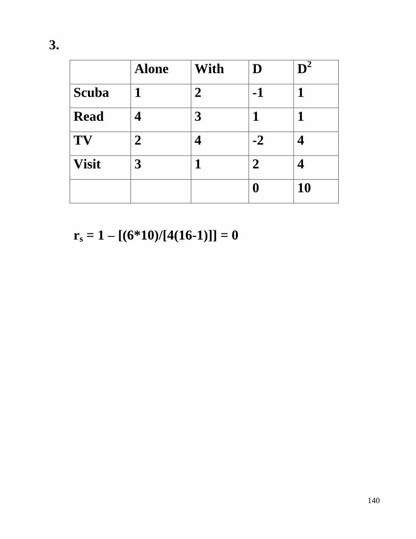
3.
Alone With D D2
Scuba 1 2 -1 1
Read 4 3 1 1
TV 2 4 -2 4
Visit 3 1 2 4
0 10
rs = 1 – [(6*10)/[4(16-1)]] = 0
141
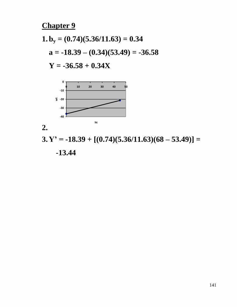
Chapter 9
1. by = (0.74)(5.36/11.63) = 0.34
a = -18.39 – (0.34)(53.49) = -36.58
Y = -36.58 + 0.34X
2.
-40
-30
-20
-10
0
0 10 20 30 40 50
ht
wt
3. Y’ = -18.39 + [(0.74)(5.36/11.63)(68 – 53.49)] =
-13.44
142
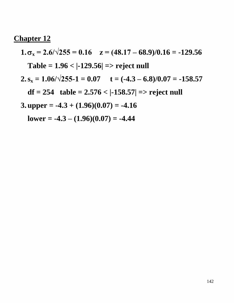
Chapter 12
1. x = 2.6/√255 = 0.16 z = (48.17 – 68.9)/0.16 = -129.56
Table = 1.96 < |-129.56| => reject null
2. sx = 1.06/√255-1 = 0.07 t = (-4.3 – 6.8)/0.07 = -158.57
df = 254 table = 2.576 < |-158.57| => reject null
3. upper = -4.3 + (1.96)(0.07) = -4.16
lower = -4.3 – (1.96)(0.07) = -4.44
143
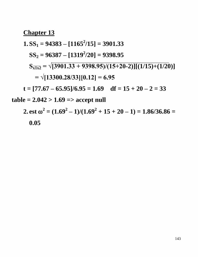
Chapter 13
1. SS1 = 94383 – [11652/15] = 3901.33
SS2 = 96387 – [13192/20] = 9398.95
Sx1x2 = √[3901.33 + 9398.95)/(15+20-2)][(1/15)+(1/20)]
= √[13300.28/33][0.12] = 6.95
t = [77.67 – 65.95]/6.95 = 1.69 df = 15 + 20 – 2 = 33
table = 2.042 > 1.69 => accept null
2. est 2 = (1.69
2 – 1)/(1.69
2 + 15 + 20 – 1) = 1.86/36.86 =
0.05
144
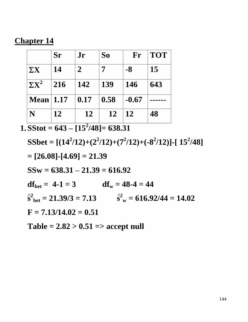
Chapter 14
Sr Jr So Fr TOT
X 14 2 7 -8 15
X2 216 142 139 146 643
Mean 1.17 0.17 0.58 -0.67 ------
N 12 12 12 12 48
1. SStot = 643 – [152/48]= 638.31
SSbet = [(142/12)+(2
2/12)+(7
2/12)+(-8
2/12)]-[ 15
2/48]
= [26.08]-[4.69] = 21.39
SSw = 638.31 – 21.39 = 616.92
dfbet = 4-1 = 3 dfw = 48-4 = 44
s2bet = 21.39/3 = 7.13 s
2w = 616.92/44 = 14.02
F = 7.13/14.02 = 0.51
Table = 2.82 > 0.51 => accept null

145
2.
1.17 0.17 0.58 -0.67
1.17 0 1 0.59 1.84
0.17 ------ 0 -0.41 0.84
0.58 ------ ------- 0 1.25
-0.67 ------ ------- ------- 0
HSD = 3.79√ 14.02/12 = 4.09
3. est2 = [21.39 – (4-1)(14.02)]/(638.31 + 14.02) = -0.03
146
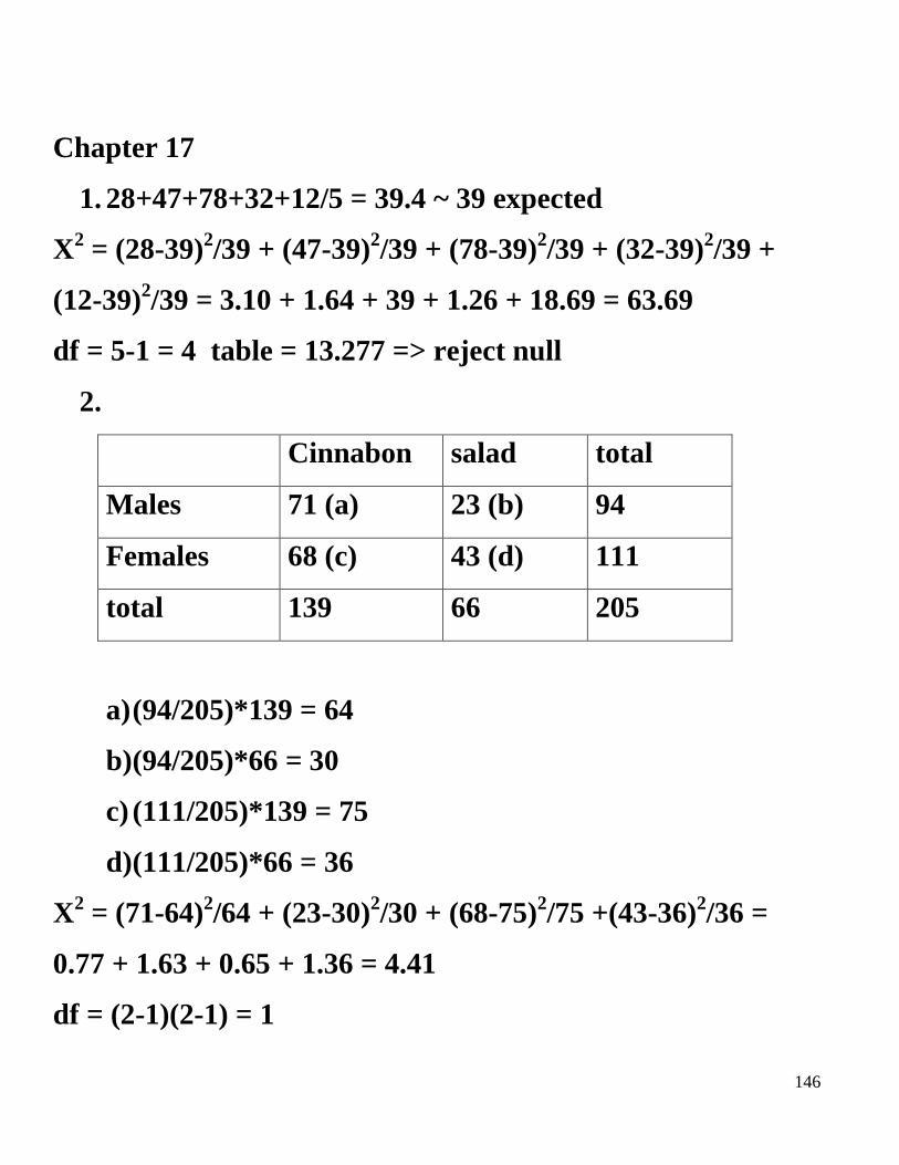
Chapter 17
1. 28+47+78+32+12/5 = 39.4 ~ 39 expected
X2 = (28-39)
2/39 + (47-39)
2/39 + (78-39)
2/39 + (32-39)
2/39 +
(12-39)2/39 = 3.10 + 1.64 + 39 + 1.26 + 18.69 = 63.69
df = 5-1 = 4 table = 13.277 => reject null
2.
Cinnabon salad total
Males 71 (a) 23 (b) 94
Females 68 (c) 43 (d) 111
total 139 66 205
a) (94/205)*139 = 64
b) (94/205)*66 = 30
c) (111/205)*139 = 75
d) (111/205)*66 = 36
X2 = (71-64)
2/64 + (23-30)
2/30 + (68-75)
2/75 +(43-36)
2/36 =
0.77 + 1.63 + 0.65 + 1.36 = 4.41
df = (2-1)(2-1) = 1
147
table = 3.841 < 4.41 => reject null