PSYCHOPHYSICS & COMPUTATIONAL MODELINGOF VISUAL MOTION PERCEPTION

Siddharth Jain

Electrical Engineering and Computer SciencesUniversity of California at Berkeley

Technical Report No. UCB/EECS-2007-97

http://www.eecs.berkeley.edu/Pubs/TechRpts/2007/EECS-2007-97.html

August 7, 2007

Copyright © 2007, by the author(s).All rights reserved.

Permission to make digital or hard copies of all or part of this work forpersonal or classroom use is granted without fee provided that copies arenot made or distributed for profit or commercial advantage and that copiesbear this notice and the full citation on the first page. To copy otherwise, torepublish, to post on servers or to redistribute to lists, requires prior specificpermission.

Psychophysics & Computational Modeling of Visual Motion Perception

by

Siddharth Jain

B.E. (Birla Institute of Technology and Science, Pilani) 2001M.S. (University of California, Berkeley) 2003

A dissertation submitted in partial satisfaction of therequirements for the degree of

Doctor of Philosophy

in

Engineering-Electrical Engineering and Computer Sciences

in the

GRADUATE DIVISIONof the

UNIVERSITY OF CALIFORNIA, BERKELEY

Committee in charge:Professor William J. Welch, Chair

Professor David T. AttwoodProfessor Donald A. Glaser

Fall 2007

The dissertation of Siddharth Jain is approved:

Chair Date

Date

Date

University of California, Berkeley

Fall 2007

Psychophysics & Computational Modeling of Visual Motion Perception

Copyright 2007

by

Siddharth Jain

1

Abstract

Psychophysics & Computational Modeling of Visual Motion Perception

by

Siddharth Jain

Doctor of Philosophy in Engineering-Electrical Engineering and Computer Sciences

University of California, Berkeley

Professor William J. Welch, Chair

The goal of the research described in this dissertation is to understand the mechanisms by

which the brain senses motion. I have performed a detailed psychophysical characterisation

of visual motion perception in general and the peculiar omega effect originally discovered

by Rose & Blake in particular in which dynamic random noise in the form of random dots

displayed in a circular annulus evokes the illusion of rotary motion. I have also found that

a model based on the Watson & Ahumada motion detector is able to explain most and

key parts of the psychophysical data such as the very delicate effects of frame duration

on motion perception, independence of observer performance on dot density in the display

and the surprising reverse phi motion caused by contrast reversing dots. In addition to

explaining the psychophysical data, the model relates reasonably well to what is known

about the neurobiology of motion sensitive cells in the brain making it a realistic model of

2

human visual motion sensing.

Some other highlights of the dissertation are as follows:

• I find that the intrinsic cortical noise in the brain which manifests itself as uncer-

tainty in motion estimation can play an important role in perception by significantly

improving detectability of subliminal motion cues at the expense of a very modest

drop in performance for a suprathreshold signal ala stochastic resonance.

• I also did experiments on observers under the influence of marijuana and found that

the THC in marijuana can cause an impairment of motion perception abilities —

observer performance decreases by as much as 15% and reaction time increases by

as much as 222±96 ms.

• I find that the observer performance is invariant to dot density in the display and argue

that this provides very powerful evidence against motion models based on matching

dots to nearest neighbors in successive frames ala (Ullman, 1979; Dawson, 1991)

etc.

• I find and prove that the rotary motion signal does not depend on the center of rotation

relative to which it is computed which explains the experimentally observed position

invariance of MST(d) cells found by (Graziano, Andersen, & Snowden, 1994).

3

Professor William J. WelchDissertation Committee Chair

i

For my mother

ii

Contents

List of Figures v

List of Tables xii

1 Introduction 11.1 Motion Perception: Psychophysics, Computational Modeling & Electro-

physiology . . . . . . . . . . . . . . . . . . . . . . . . . . . . . . . . . . . 11.2 Overview of the dissertation . . . . . . . . . . . . . . . . . . . . . . . . . 6

2 Psychophysical investigation of visual motion perception 112.1 Introduction . . . . . . . . . . . . . . . . . . . . . . . . . . . . . . . . . . 112.2 Stimulus & Methods . . . . . . . . . . . . . . . . . . . . . . . . . . . . . 142.3 Effect of dot correlation, frame duration, dot density and annulus size on χ

and τ . . . . . . . . . . . . . . . . . . . . . . . . . . . . . . . . . . . . . 202.3.1 Effect of dot correlation c . . . . . . . . . . . . . . . . . . . . . . 202.3.2 Effect of frame duration fd . . . . . . . . . . . . . . . . . . . . . 212.3.3 Effect of dot density dd . . . . . . . . . . . . . . . . . . . . . . . . 242.3.4 Effect of angle subtended by inner circle ic . . . . . . . . . . . . . 252.3.5 Effect on the reaction time τ . . . . . . . . . . . . . . . . . . . . . 26

2.4 The Omega Effect and reproducibility of observer response . . . . . . . . . 282.5 Thresholds on motion perception . . . . . . . . . . . . . . . . . . . . . . . 342.6 Can an observer tell apart c = 0 from c = 0.1? . . . . . . . . . . . . . . . . 352.7 What happens if only a sector of the complete racetrack is made visible? . . 372.8 Non-uniformly vs. Uniformly distributed motion cues . . . . . . . . . . . . 392.9 Effect of different types of correlation . . . . . . . . . . . . . . . . . . . . 422.10 Conclusion . . . . . . . . . . . . . . . . . . . . . . . . . . . . . . . . . . 45

3 Modeling visual motion perception: Motion Correspondence vs. a Correspon-denceless model 473.1 Introduction . . . . . . . . . . . . . . . . . . . . . . . . . . . . . . . . . . 47

iii

3.2 Model Description . . . . . . . . . . . . . . . . . . . . . . . . . . . . . . 483.2.1 Nearest Neighbor (NN) Model . . . . . . . . . . . . . . . . . . . . 483.2.2 Model2: a correspondenceless model . . . . . . . . . . . . . . . . 54

3.3 Results . . . . . . . . . . . . . . . . . . . . . . . . . . . . . . . . . . . . . 543.3.1 Effect of dot correlation c . . . . . . . . . . . . . . . . . . . . . . 543.3.2 Effect of frame duration fd . . . . . . . . . . . . . . . . . . . . . 553.3.3 Effect of annulus width . . . . . . . . . . . . . . . . . . . . . . . . 563.3.4 Effect of dot density dd . . . . . . . . . . . . . . . . . . . . . . . . 583.3.5 Effect of hop size h . . . . . . . . . . . . . . . . . . . . . . . . . . 603.3.6 Model Sensitivity to center position . . . . . . . . . . . . . . . . . 633.3.7 Effect of displaying only a sector . . . . . . . . . . . . . . . . . . 673.3.8 The omega effect . . . . . . . . . . . . . . . . . . . . . . . . . . . 693.3.9 Reproducibility of observer responses . . . . . . . . . . . . . . . . 71

3.4 Limitations of models . . . . . . . . . . . . . . . . . . . . . . . . . . . . . 743.5 Conclusions and Remarks . . . . . . . . . . . . . . . . . . . . . . . . . . . 77

4 An introduction to the Watson-Ahumada (WA) motion detector 814.1 At what rate should motion be sampled to make apparent motion indistin-

guishable from continuous motion? . . . . . . . . . . . . . . . . . . . . . . 934.2 Why can’t we see things that move too slowly or too fast? . . . . . . . . . . 1024.3 Gradient based approaches . . . . . . . . . . . . . . . . . . . . . . . . . . 1044.4 Conclusion . . . . . . . . . . . . . . . . . . . . . . . . . . . . . . . . . . 1064.5 Appendix 1: Effect of convolution with a Gabor . . . . . . . . . . . . . . . 107

5 Modeling visual motion perception with the Watson-Ahumada (WA) motiondetector 1085.1 Introduction . . . . . . . . . . . . . . . . . . . . . . . . . . . . . . . . . . 1085.2 Model Description . . . . . . . . . . . . . . . . . . . . . . . . . . . . . . 1095.3 Results . . . . . . . . . . . . . . . . . . . . . . . . . . . . . . . . . . . . . 114

5.3.1 Stochastic Resonance effects . . . . . . . . . . . . . . . . . . . . . 1145.3.2 The Omega effect . . . . . . . . . . . . . . . . . . . . . . . . . . . 1155.3.3 Effect of dot correlation c . . . . . . . . . . . . . . . . . . . . . . 1195.3.4 Reverse Phi motion . . . . . . . . . . . . . . . . . . . . . . . . . . 1205.3.5 Effect of frame duration fd . . . . . . . . . . . . . . . . . . . . . 1265.3.6 Effect of dot density dd . . . . . . . . . . . . . . . . . . . . . . . . 1325.3.7 Effect of annulus width ic . . . . . . . . . . . . . . . . . . . . . . 1325.3.8 Effect of hop size h . . . . . . . . . . . . . . . . . . . . . . . . . . 1355.3.9 Effect of inserting random frames . . . . . . . . . . . . . . . . . . 1355.3.10 Model Sensitivity to center position . . . . . . . . . . . . . . . . . 1365.3.11 Effect of displaying only a sector . . . . . . . . . . . . . . . . . . 1395.3.12 Dipoles . . . . . . . . . . . . . . . . . . . . . . . . . . . . . . . . 140

5.4 Conclusion . . . . . . . . . . . . . . . . . . . . . . . . . . . . . . . . . . 149

iv

6 THC induced impairment of visual motion perception 1526.1 Introduction . . . . . . . . . . . . . . . . . . . . . . . . . . . . . . . . . . 1526.2 Data collection procedures . . . . . . . . . . . . . . . . . . . . . . . . . . 1546.3 Results . . . . . . . . . . . . . . . . . . . . . . . . . . . . . . . . . . . . . 155

6.3.1 Timecourse of metabolites & effect of THC on observer performance1556.3.2 Building a classifier to detect drug use . . . . . . . . . . . . . . . . 166

6.4 Conclusion . . . . . . . . . . . . . . . . . . . . . . . . . . . . . . . . . . 1716.5 Acknowledgements . . . . . . . . . . . . . . . . . . . . . . . . . . . . . . 172

7 Conclusion 173

References 177

v

List of Figures

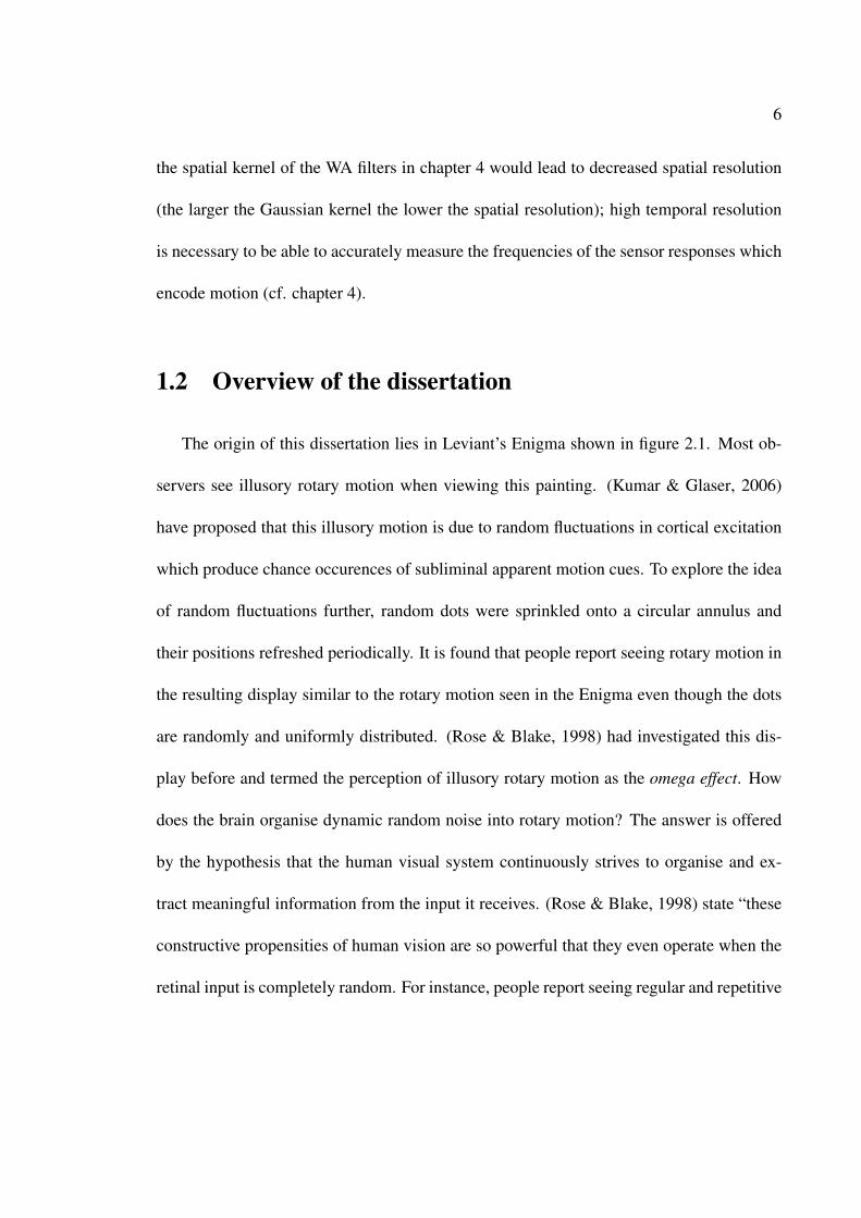
2.1 Enigma painting by I. Leviant. Most observers can see illusory rotary mo-tion in the rings. . . . . . . . . . . . . . . . . . . . . . . . . . . . . . . . . 12

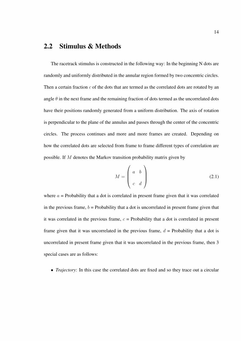
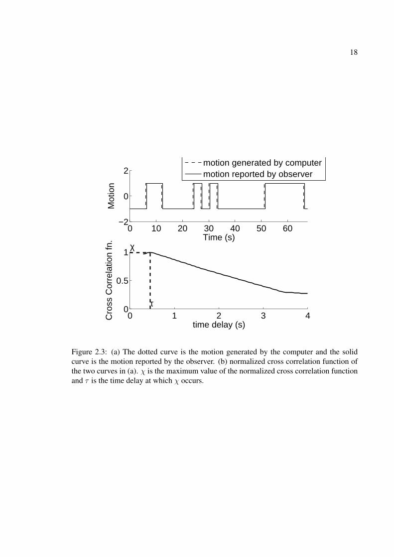
2.2 A few frames of the racetrack stimulus (resized to fit on page). . . . . . . . 172.3 (a) The dotted curve is the motion generated by the computer and the solid

curve is the motion reported by the observer. (b) normalized cross corre-lation function of the two curves in (a). χ is the maximum value of thenormalized cross correlation function and τ is the time delay at which χoccurs. . . . . . . . . . . . . . . . . . . . . . . . . . . . . . . . . . . . . . 18

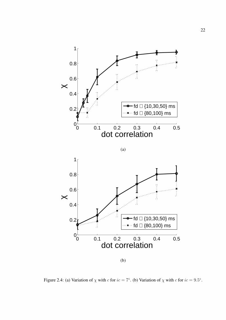
2.4 (a) Variation of χ with c for ic = 7◦. (b) Variation of χ with c for ic = 9.5◦. 222.5 χ vs. frame duration fd. c = 0.1, dd = 5, ic = 7◦. fd ∼ 30ms is found to

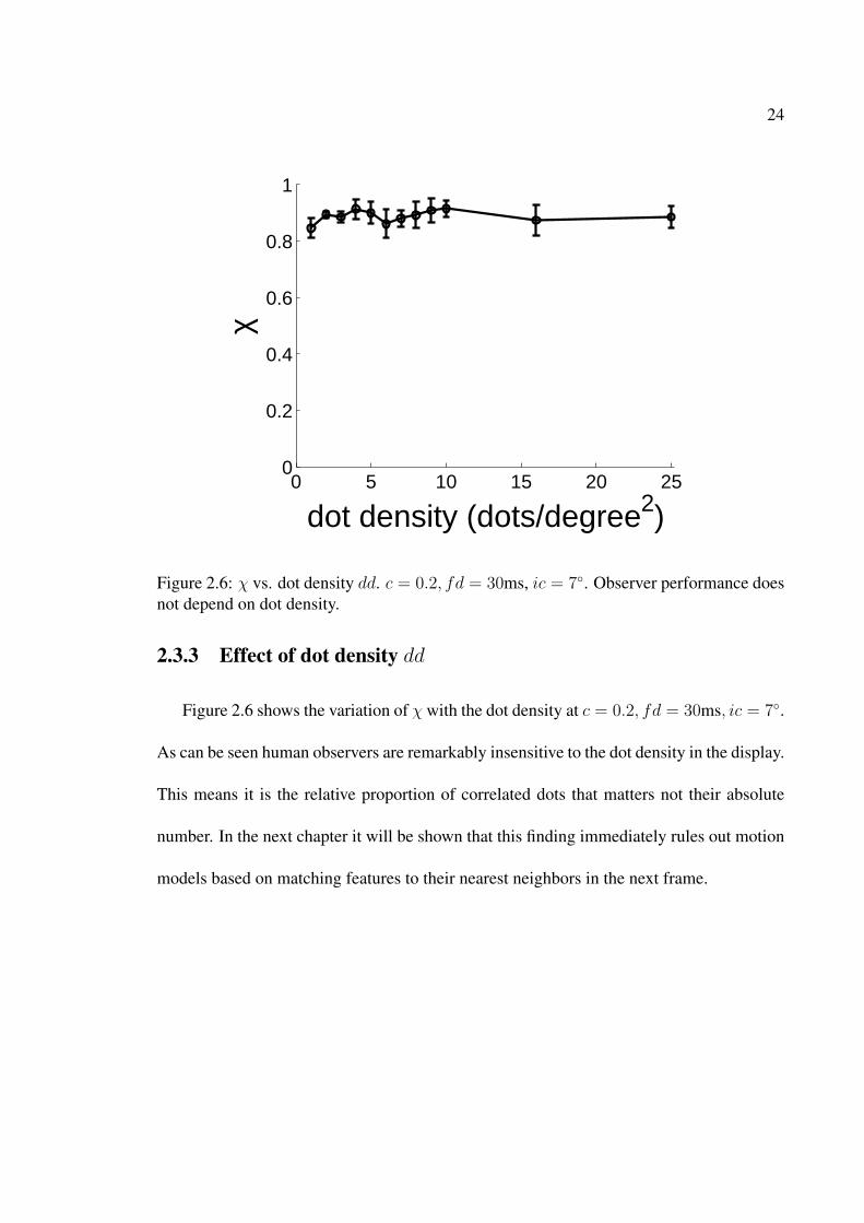
be optimal for motion perception. . . . . . . . . . . . . . . . . . . . . . . 232.6 χ vs. dot density dd. c = 0.2, fd = 30ms, ic = 7◦. Observer performance

does not depend on dot density. . . . . . . . . . . . . . . . . . . . . . . . . 242.7 Plot of χ vs. ic for c = 0.1, dd = 5, fd = 30 ms. . . . . . . . . . . . . . . . 252.8 Scatter plot of τ vs. χ for 4 observers together with a piecewise linearized

fit. At high χ, τ is around 0.5s with little variation. As χ decreases τ aswell as its variation increase. . . . . . . . . . . . . . . . . . . . . . . . . . 26

2.9 Plot of τ vs. c at ic = 7◦ . . . . . . . . . . . . . . . . . . . . . . . . . . . 272.10 Response curves of an observer to the same stimulus in 6 trials (c = 0.03, dd =

5, fd = 30 ms, ic = 7◦) . . . . . . . . . . . . . . . . . . . . . . . . . . . 302.11 Cross correlation function of first two response curves in Figure 2.10. ζ is

defined as maximum value of the cross correlation function . . . . . . . . . 312.12 Plot of ζ vs. c for 4 observers. fd = 30 ms, dd = 5, ic = 7◦. . . . . . . . . 322.13 (a) histogram of Inter Flip Interval (IFI) at c = 0. (b) normalised histogram

of ln(IFI) together with a Gaussian fit (black curve). . . . . . . . . . . . . . 332.14 A frame in which only a 60◦ sector of the racetrack is made visible. . . . . 372.15 Plot of χ vs. c when only a sector of the racetrack is made visible. . . . . . 382.16 Plot showing fraction of correlated dots that lie outside the sector using the

modified racetrack algorithm . . . . . . . . . . . . . . . . . . . . . . . . . 40

vi

2.17 χ vs. c for three cases (i) normal racetrack, (ii) modified racetrack, (iii)modified racetrack and the observers are given a hint that they may seemotion more clearly if they pay more attention to a sector of the racetrack . 43

2.18 Effect of type of correlation used on observer performance. . . . . . . . . . 44

3.1 Two successive frames of the racetrack superimposed on each other. Thedots in the first frame are colored red and the dots in the second frameare colored blue. (b) illustration of pairings obtained after nearest neigh-bor (NN) matching. The spurious matches indicated by the long lines arediscounted by the spatial weighting function w in equation 3.2 . . . . . . . 52

3.2 Flowchart for the Nearest Neighbor (NN) model . . . . . . . . . . . . . . . 523.3 NN model response at c=0.1, fd=30ms, ic=7◦, dd=2.5 dots/deg2 . . . . . . 533.4 χ vs. dot correlation c. Comparison of human and model performance.

fd=30ms, ic=7◦, dd=5 dots/deg2. Throughout the chapter length of error-bars is equal to 1 standard deviation unless otherwise stated. Although theNN model appears better, by addition of suitable amount of noise the curvefor Model2 can be made to fall to fit the psychophysical data more closely. . 55

3.5 χ vs. frame duration (fd). For human observers fd=30ms is about optimumwhereas the models show steady improvement in χ as fd is decreased. Thedecrease in χ for humans at fd<30ms may be explained by humans expe-riencing an information overload. c=0.1, ic=7◦, dd=5 dots/deg2 . . . . . . . 57

3.6 χ vs. angle subtended by inner circle (ic). c=0.1, fd=30ms, dd=5 dots/deg2,angle subtended by outer circle fixed at 10◦. . . . . . . . . . . . . . . . . . 59

3.7 χ vs. dot density (dd). Human observers and model2 are insensitive todot density whereas the NN model and its variants have a marked depen-dence on dot density as dictated by the probability of mismatch (see textfor details). c=0.2, fd=30ms, ic=7◦. . . . . . . . . . . . . . . . . . . . . . . 61

3.8 χ vs. hop size for various dot densities. c=0.4, fd=30ms, ic=7◦. (a,b) NNmodel (c,d) humans (e,f) Model2 . . . . . . . . . . . . . . . . . . . . . . . 64

3.9 Point O represents the true center of rotation whereas point C is the centerrelative to which rotary motion is computed by the model. The offset isgiven by ~OC

Riwhere Ri is radius of inner circle. . . . . . . . . . . . . . . . . 66

3.10 χ vs. center relative to which rotary motion is computed. For both modelsthe center position does not matter. This may explain the experimentallyobserved position invariance of MST(d) cells. c=0.1, fd = 30 ms, ic = 7◦,dd = 2.5 dots/deg2. (a) full 360◦ of the annulus is visible. (b) only 90◦ ofthe annulus is made visible; type1 — a single 90◦ sector of the racetrack ismade visible, type2 — two diametrically opposite located sectors each 45◦

in size are made visible . . . . . . . . . . . . . . . . . . . . . . . . . . . . 67

vii

3.11 χ vs. sector. In case of type 1 only one sector is displayed whereas in caseof type 2 two diametrically opposite located sectors (each half the size ofthe sector in type 1) are displayed. (a) human performance c = 0.3, (b)model performance c = 0.1. . . . . . . . . . . . . . . . . . . . . . . . . . 68

3.12 c = 0 (a) waveform of I at fd = 30 ms (b) waveform of I at fd = 80 ms (c)fraction of time γ for which rotary motion is perceived by human observers. 71

3.13 As the width of annulus is decreased amount of rotary motion increasesand amount of radial motion decreases. Model2 c = 0, fd = 30 ms, dd =2.5 dots/degree2, outer circle=10◦. . . . . . . . . . . . . . . . . . . . . . . 72

3.14 Variation of ζ which is a measure of response reproducibility for a givenstimulus vs. dot correlation c. . . . . . . . . . . . . . . . . . . . . . . . . . 74

3.15 Effect of uncertainty in positions of dots for the two models. (a) NN, (b)Model 2. c=0.5, fd=30ms, ic=7◦. . . . . . . . . . . . . . . . . . . . . . . . 77

3.16 Effect of inserting K random frames between correlated frames for humanobservers. χ does not drop to zero level abruptly for non-zero K show-ing that human observers do not match just the consecutive 2 frames butmultiple frames are taken into consideration. (a) χ vs. K for different dotcorrelation, fd=30ms. (b) χ vs. K for different frame duration, c = 0.5. . . . 77

4.1 A motion detection algorithm takes as input a spatiotemporal movie L(x, y, t)and outputs the instantaneous image velocity at every position (x, y) andtime t denoted by (vx(x, y, t), vy(x, y, t)). The velocity (vx, vy) at a partic-ular position (x0, y0) and time instant t0 is determined by the input signalcontained within a small causal spatiotemporal patch or window centeredat (x0, y0, t0). . . . . . . . . . . . . . . . . . . . . . . . . . . . . . . . . . 82

4.2 The fourier transform of a stationary image lies on the ωxωy plane and isdenoted by the solid plane. The effect of motion is to shear the fouriertransform so that it now lies on the plane ωxvx + ωyvy + ωt = 0. Thearrows indicate the displacement of a single spatial-frequency component(a sine grating). . . . . . . . . . . . . . . . . . . . . . . . . . . . . . . . . 87

4.3 The WA motion detection pipeline. The input is first convolved through anumber of filters in parallel. The temporal frequencies of filter responsescontain information about the velocity as per equation 4.19. The filter re-sponses have to be pooled to estimate the motion. . . . . . . . . . . . . . . 89

4.4 Power spectra of the filters in figure 4.3. Each different color correspondsto a different filter. Only the +ve half of ωt space is shown. Since thefilters model V1 simple cells and therefore must have real valued impulseresponses the power spectra in −ve half of ωt can be obtained using theidentity P (ωx, ωy, ωt) = P (−ωx,−ωy,−ωt). . . . . . . . . . . . . . . . . 90

4.5 Optical flow at 1/4 cycles/pixel or 10.275 cycles/degree in response to aradially expanding random dot stimulus. . . . . . . . . . . . . . . . . . . . 94

viii

4.6 Optical flow at 1/8 cycles/pixel or 5.13 cycles/degree in response to a radi-ally expanding random dot stimulus. . . . . . . . . . . . . . . . . . . . . . 95

4.7 Optical flow at 1/16 cycles/pixel or 2.56 cycles/degree in response to aradially expanding random dot stimulus. . . . . . . . . . . . . . . . . . . . 96

4.8 Optical flow at 1/32 cycles/pixel or 1.28 cycles/degree in response to aradially expanding random dot stimulus. . . . . . . . . . . . . . . . . . . . 97

4.9 Optical flow at 1/64 cycles/pixel or 0.64 cycles/degree in response to aradially expanding random dot stimulus. . . . . . . . . . . . . . . . . . . . 98

4.10 x− t spacetime plots for a particle moving with constant velocity (a) con-tinuous motion (b) stroboscopic motion (c) staircase motion . . . . . . . . 99

4.11 Response of a motion-sensitive cell as a particle moves across its receptivefield. Velocity of particle = v. Spatial size of receptive field = L. Temporalsize of receptive field = T . (a) v � L/T (b) v ∼ L/T (c) v � L/T . . . . . 103

5.1 (a) Block schematic of the model (b) Optical flow (c) Model response atvarious other stages in the pipeline . . . . . . . . . . . . . . . . . . . . . . 110

5.2 Variation of model reproducibility with noise at c = 0. The dotted linerepresents the threshold below which ζ values can be taken to imply zeroreproducibility. . . . . . . . . . . . . . . . . . . . . . . . . . . . . . . . . 113

5.3 (a) variation of χ with noise at c = 0.05 with fixed threshold; SR can beseen, (b) variation of χ with noise at c = 0.05 with variable threshold, (c) χvs. noise at c = 0.02 with fixed threshold; no SR occurs because the signalis already well above threshold . . . . . . . . . . . . . . . . . . . . . . . . 115

5.4 Waveform of I at c = 0. It is a zero mean signal consistent with the factthat c = 0 or the dots are randomly and uniformly distributed. Howeverthere are fluctuations about zero and whenever these fluctuations cross athreshold a perception of rotary motion corresponding to the omega effectcan occur. . . . . . . . . . . . . . . . . . . . . . . . . . . . . . . . . . . . 117

5.5 σ(I) at c = 0. For ic < 6◦ the rotary and radial motions cancel out and theomega effect disappears whereas for ic > 8◦ the rotary motion and hencethe omega effect becomes increasingly dominant. . . . . . . . . . . . . . . 118

5.6 Response reproducibility ζ vs. c. Both model and humans show zero re-producibility at c = 0 and the reproducibility steadily increases with c asthe motion signal gets stronger and more impervious to noise. . . . . . . . 119

5.7 (a) χ vs. c (b) τ vs. c. fd=30 ms, ic = 7◦, dd = 5 dots/deg2 . . . . . . . . . 1205.8 χ vs. c for contrast reversing dots. χ is defined here as the minimum value

of the normalized cross correlation function between input and responsewithin a window of [0,4]s. fd=30 ms, ic = 7◦, dd = 2.5 dots/deg2 . . . . . 124

ix

5.9 (a) I(x, t) profile of a 1D contrast reversing particle moving with velocityv. (b) I(ωx, ωt) is zero everywhere except at vωx + ωt = nω0 where nis a non-zero integer and ω0 = 2π

Twith T being the period of the square

wave in (a). The dotted square denotes the window of visibility. The threelarge dots are meant to indicate the presence of an infinite number of linesgiven by the equation vωx + ωt = nω0 where n is a non-zero integer. TheWA motion detector would fit a line that (i) passes through the origin, (ii)captures as much energy as possible of I(ωx, ωt) . . . . . . . . . . . . . . 125

5.10 (a) spacetime plot of a pattern of random black and white bars moving tothe right. The spacetime plot displays a very strong orientation/tilt whichis the characteristic signature of motion. (b) the bars move to the right butalso reverse their polarity as they move i.e. black changes to white andvice-versa. (c),(d) show power spectrum of (a),(b) respectively togetherwith best fitting line that passes through the origin (indicated in red) . . . . 127

5.11 χ vs. frame duration fd. c=0.1, ic = 7◦, dd = 5 dots/deg2 . . . . . . . . . . 1285.12 Explanation of the fd effect. Motion sensitive cells in the brain are sensi-

tive to motion within a window of 200 ms. The input signal changes afterevery fd seconds. Three cases are illustrated. (a) In this case the input ismostly constant within a window of 200 ms and so motion sensitive cellswill fail to detect any motion (b) fd ∼ 30 ms provides the right amountof fd for optimal response of motion sensitive cells (c) when fd is toosmall the input changes at a rate greater than the maximum rate the cell canhandle; things appear washed out in this case. . . . . . . . . . . . . . . . . 130

5.13 χ vs. dot density dd. c=0.2, ic = 7◦, fd = 30 ms . . . . . . . . . . . . . . 1335.14 χ vs. angle subtended by inner circle diameter ic. Angle subtended by

outer circle diameter is fixed at 10◦. c=0.1, dd = 5 dots/deg2, fd = 30 ms . 1345.15 (a) χ vs. hop size for human observers (b) χ vs. hop size for model.

c = 0.4, fd = 30 ms, ic = 7◦. . . . . . . . . . . . . . . . . . . . . . . . . 1365.16 Effect of inserting K random frames between correlated frames. c = 0.5,

fd = 10 ms, dd = 5 dots/degree2, ic = 7◦. . . . . . . . . . . . . . . . . . . 1375.17 χ vs. center relative to which rotary motion is computed. χ values are not

affected much by uncertainty in knowledge of true center position and startto deteriorate only when the offset becomes very large. This may explainthe experimentally observed position invariance of MST(d) cells. c=0.1,fd = 30 ms, ic = 7◦, dd = 2.5 dots/deg2. (a) full 360◦ of the annulus isvisible. (b) only 90◦ of the annulus is made visible; type1 — a single 90◦

sector of the racetrack is made visible, type2 — two diametrically oppositelocated sectors each 45◦ in size are made visible . . . . . . . . . . . . . . . 138

5.18 χ vs. sector. In case of type 1 only one sector is displayed whereas in caseof type 2 two diametrically opposite located sectors (each half the size ofthe sector in type 1) are displayed. (a) human performance c = 0.3, (b)model performance c = 0.1. . . . . . . . . . . . . . . . . . . . . . . . . . 139

x

5.19 (a) tangential dipoles with spacing = 12 minutes (b) radial dipoles withspacing = 12 minutes . . . . . . . . . . . . . . . . . . . . . . . . . . . . . 140

5.20 A dipole is formed by two dots — one black and one white. The separationbetween the dots is known as dipole spacing. When the spacing is zero thedots are touching each other. . . . . . . . . . . . . . . . . . . . . . . . . . 141

5.21 (a) χ vs. dipole spacing for experiment r = 1 (b) χ vs. dipole spacing formodel bwir = 1 . . . . . . . . . . . . . . . . . . . . . . . . . . . . . . . . 143

5.22 (a) χ vs. dipole spacing for experiment r = 10 (b) χ vs. dipole spacing formodel bwir = 10 . . . . . . . . . . . . . . . . . . . . . . . . . . . . . . . 146

5.23 Two kinds of motion cues that occur with tangential dipoles RC ON. Twosuccessive frames are shown superimposed on each other. The white dotsare effectively invisible at r = 10. (a) black dots are separated by h + d (b)black dots are separated by h− d where h is the hop size (the displacementgiven to the dipole in the next frame) and d is the center-to-center spacingof the dipole. Motion should reverse when d > h. . . . . . . . . . . . . . . 147

5.24 Two kinds of motion cues that occur with radial dipoles RC ON. Two suc-cessive frames are shown superimposed on each other. The white dots areeffectively invisible at r = 10. h is the hop size (the displacement givento the dipole in the next frame) and d is the center-to-center spacing ofthe dipole. When d becomes comparable to or greater than h these twoconfigurations together should give a sensation of pulsating radial motion. . 148

5.25 (a) χ vs. r for experiment (b) χ vs. bwir for model. dipole spacing = 1minute in both cases . . . . . . . . . . . . . . . . . . . . . . . . . . . . . . 149

6.1 Timecourse of ∆9 THC in blood plasma. Data from 11 subjects. Errorbarsare ± s.e.m. . . . . . . . . . . . . . . . . . . . . . . . . . . . . . . . . . . 157

6.2 Timecourse of CBD in blood plasma. Data from 11 subjects. Errorbars are± s.e.m. . . . . . . . . . . . . . . . . . . . . . . . . . . . . . . . . . . . . 158

6.3 Timecourse of CBN in blood plasma. Data from 11 subjects. Errorbars are± s.e.m. . . . . . . . . . . . . . . . . . . . . . . . . . . . . . . . . . . . . 159

6.4 Timecourse of 11-OH-THC in blood plasma. Data from 11 subjects. Er-rorbars are ± s.e.m. . . . . . . . . . . . . . . . . . . . . . . . . . . . . . 160

6.5 Timecourse of THCCOOH in blood plasma. Data from 11 subjects. Error-bars are ± s.e.m. . . . . . . . . . . . . . . . . . . . . . . . . . . . . . . . 161

6.6 Plot of χ vs. c. Data from 11 subjects. The numbers {0, 1.7, 3.4, 6.8}indicate % THC administered. The letters {v, s} indicate the method ofdrug delivery — through vapor or smoke. Errorbars are ± s.e.m. . . . . . . 162

6.7 Plot of χ vs. c with and without drug. Data from 11 subjects. Errorbars are± s.e.m. . . . . . . . . . . . . . . . . . . . . . . . . . . . . . . . . . . . . 163

6.8 Plot of χ vs. c. Data from 11 subjects. The numbers {0, 1.7, 3.4, 6.8}indicate % THC administered. Errorbars are ± s.e.m. . . . . . . . . . . . . 164

xi

6.9 Plot of χ vs. c. Data from 11 subjects. The letters {v, s} indicate themethod of drug delivery — through vapor or smoke. Errorbars are ± s.e.m. 165

6.10 Plot of τ vs. c with and without drug. Data from 11 subjects. Errorbars are± s.e.m. . . . . . . . . . . . . . . . . . . . . . . . . . . . . . . . . . . . . 167

6.11 Plot of τ vs. χ. Data from 11 subjects. Errorbars are ± s.e.m. . . . . . . . 168

xii

List of Tables

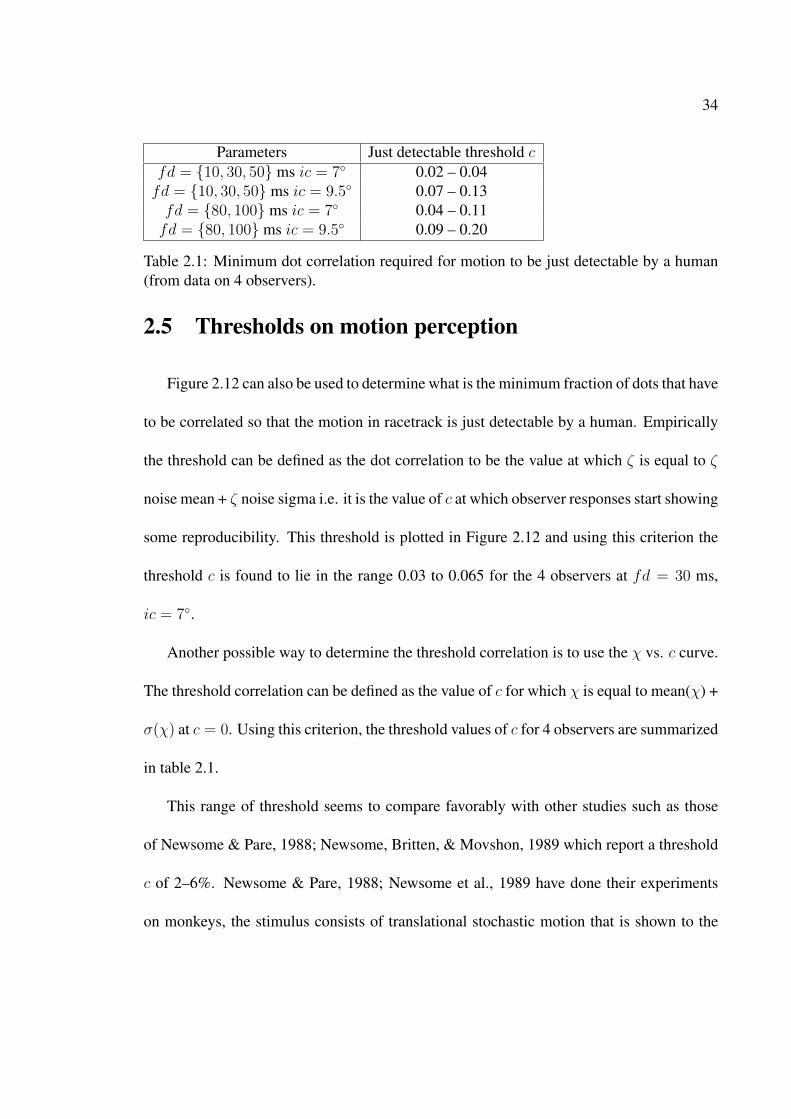
2.1 Minimum dot correlation required for motion to be just detectable by ahuman (from data on 4 observers). . . . . . . . . . . . . . . . . . . . . . . 34

2.2 A test in which observers are asked to classify whether or not the racetrackhas any embedded correlation in it. . . . . . . . . . . . . . . . . . . . . . . 36

6.1 Mean, s.e.m., t-statistic and P value for THC concentration (ng/ml) undervapor and smoke. The P value is the probability of observing the observeddifference in means or even more extreme by chance assuming the nullhypothesis is true — that there is no difference in the concentration of THCdelivered by vapor and smoke. Small values of P cast doubt on the validityof the null hypothesis. . . . . . . . . . . . . . . . . . . . . . . . . . . . . . 156

6.2 τ1 is reaction time (in seconds) without drug and τ2 is reaction time (inseconds) under the influence of drug. Mean(d) = 0.222s, std(d) = 0.0957s. . 166

xiii

List of Symbols and Abbreviations

χ observer performance

τ reaction time

ζ reproducibility of response

c dot correlation = number of correlated dotstotal number of dots

dd dot density

fd frame duration — the length of time for which a frame stays on the screen

h hop size

ic angle subtended by inner circle diameter at the eye

MST medial superior temporal

MSTd dorsal medial superior temporal

MT middle temporal cortex

xiv

RF receptive field

V1 primary visual cortex

xv

Acknowledgments

There are many people who have contributed to this dissertation. I would like to begin

by thanking my advisor Professor Donald A. Glaser who gave me an opportunity to work

in his lab under his close supervision and for providing me with much needed financial

support through a period of approximately two and a half years without which I would not

have been able to complete my studies. Thanks are due to Dr. T. Kumar, Professor Glaser’s

close colleague, who guided me through the psychophysical experiments and acted much

like a surrogate advisor and mentor. Professors Jack Welch and David Attwood have been

very kind to serve on my dissertation committee and have generously given me much of

their valuable time and accepted many of my requests. In particular thanks are due to

Professor Jack Welch for agreeing to serve as my EE co-advisor.

I wish to thank all the students in Professor Glaser’s lab with whom my stay overlapped:

Davis Barch, Kirill Shokirev, Mike Wahl, Sebum Paik, Tim Erlenmeyer. Many thanks are

due to the many subjects who generously participated in our research and gave us valuable

psychophysical data. I am very grateful to Ruth Gjerde & Mary Byrnes at the EE Graduate

Student Affairs Office for their help and support at all stages of my grad student life. I also

need to give a big thank you to Berkeley EECS for accepting me into their PhD program

which was a dream come true for me.

Finally the people that matter the most: my friends and family. I dedicate this disserta-

tion to my mother who has given me unconditional love and suffered much because of me.

Thanks are due to my brother who took care of my mother while I have been away from

xvi

home all these years. I can never thank enough my uncles Anil & Surendra Tauji, Vicky

Bhaiya and their families for the unconditional love and support they have always showered

on me. Indeed I think my family is my biggest asset. Thanks are also due to all my paternal

uncles, aunts and their families for their love and support: Rajiv, Rakesh, Sanjeev, Sunil

Mamaji. A big thank you to Babusha and Alok for their tremendous help and support and

without whom my life in Berkeley would have been dull beyond my imagination; I will

sorely miss you. I also thank Ali & Fatema, David Gelbart, Arindam Chakrabarti, Alex

Aris, Sudarshan Rajan and all other friends I made at Berkeley. My apologies to anyone I

have overlooked!

Life as a grad student was not easy for me. I am glad its finally over.

Only after disaster can we be resurrected

1

Chapter 1

Introduction

1.1 Motion Perception: Psychophysics, Computational Mod-

eling & Electrophysiology

Motion perception is an important task performed by the human visual system. It has

been extensively studied psychophysically, electrophysiologically and computationally for

more than 35 years now. For recent reviews on the topic see e.g. (Grzywacz & Merwine,

2003; Derrington, Allen, & Delicato, 2004). It is of course impossible to acknowledge

and mention each and every development in a few pages and the following paragraphs are

intended to provide an introduction and discussion of some of the most important results in

the literature with particular relevance to the research work presented in this dissertation.

Most psychophysical studies of motion perception including the experiments described

in this dissertation are done using the so called apparent motion displays in which a series of

2

image frames are displayed one after the other on a computer monitor in rapid succession;

essentially the underlying continuous-time signal is sampled and the sampling period is

termed as the frame duration. For example, if we consider a moving dot the successive

frames will display the dot at positions t1, t2, t3, · · · where ti are the times at which motion

is sampled. The frame duration can be further divided into two times — a time for which

the frame is ON and a time for which the frame is OFF and the screen is blank. The OFF

time is zero throughout the experiments described in this dissertation.

One of the earliest psychophysical studies of visual motion perception is the book by

(Kolers, 1972); also see (Anstis, 1980; Anstis & Rogers, 1975; Sperling, 1976; Ross &

Burr, 1983) for some other early papers on motion psychophysics. Early psychophysical

studies of motion perception involved only a few dots — in such cases the motion seen by

the observer could be explained by trying to match a dot to appropriate partner(s) in the next

frame; most commonly the partner is the nearest neighbor (NN) in the next frame. This

spawned the idea of motion correspondence and led to the development of the minimal

mapping theory of (Ullman, 1979). (Dawson, 1991) postulated three principles to guide

motion correspondence: (i) the sum of path lengths should be minimised (ii) each dot

should try to match to a unique partner in the next frame; thus splitting and fusing of dots

should be avoided; this is known as the element integrity principle (iii) all dots should

tend to move in the same direction; known as the relative velocity principle. However as

I will argue in this dissertation models based on motion correspondence in the sense of

finding a matching partner for each dot in the next frame are fundamentally flawed and

3

their limitations become obvious as the number of dots in the display is increased.

(Williams & Sekuler, 1984) described psychophysical experiments on stochastic trans-

lational motion stimuli. A screen filled with random dots undergoing Brownian motion in

all 360◦ directions with equal probability appears as random noise. However if the range

of motion is restricted to a range less than 360◦ the pattern would appear to flow en masse

in the direction of the mean of the distribution, even though the individual perturbations of

the dots was still evident. Random Dot Kinematograms (RDKs) undergoing translational

motion have been used very successfully by Newsome & colleagues to firmly establish the

important role played by area MT in motion perception. In 1998 (Rose & Blake, 1998)

reported that although a screen filled with dynamic random dots appears as random noise,

if the dots are displayed in a circular annulus the display evokes a perception of rotary

motion even though no motion is embedded in the stimulus. They termed the phenomenon

as the omega effect. It is the c = 0 case of our racetrack stimulus and will be extensively

discussed in the dissertation.

Some of the earliest algorithms for motion detection appeared in the computer vision lit-

erature where this problem is more commonly referred to as optical flow (Lucas & Kanade,

1981; Horn & Shunck, 1981). These classic algorithms are still used in many machine

vision applications the most ubiquitous being the optical mouse we use everyday. Three

seminal papers modeling human visual motion perception appeared as (Adelson & Bergen,

1985; Santen & Sperling, 1985; Watson & Ahumada, 1985). Chapter 4 provides an in-

troduction to the (Watson & Ahumada, 1985) model which is used in this dissertation to

4

model the psychophysics of the racetrack. (Heeger, 1987; E. Simoncelli & Heeger, 1998)

made notable extensions to the earlier work of (Adelson & Bergen, 1985) which can detect

only 1D motion. Most recently (Rust, Mante, Simoncelli, & Movshon, 2006) have put

forward a model that captures the full range of pattern motion selectivity found in MT and

builds on the earlier work of (E. Simoncelli & Heeger, 1998). Since the work of (Lucas

& Kanade, 1981; Horn & Shunck, 1981) papers and reviews on optical flow continue to

appear regularly in the computer vision literature.

Electrophysiological studies indicate the presence of a motion pathway V1→MT→MST(d)

in the brain. Recent studies have also found a small percentage of neurons that are directly

connected from LGN to MT bypassing V1 (Sincich, Park, Wohlgemuth, & Horton, 2004).

The studies of (DeAngelis, Ohzawa, & Freeman, 1993, 1995, 1996) have found that mo-

tion sensitive neurons are characterised by an oriented spacetime receptive field (RF) struc-

ture which is the essence of motion and is predicted by the Watson-Ahumada (WA) and

Adelson-Bergen (AB) motion perception theories. The studies by (Van Essen, Maunsell, &

Bixby, 1981; Maunsell & Van Essen, 1981b, 1981a; Felleman & Kaas, 1984; Newsome &

Pare, 1988) established the important role played by area MT in motion perception; for a

recent review of what does MT do see (Born & Bradley, 2005). Majority of MT neurons are

direction and speed selective with the average cell firing rate more than ten times stronger

to motion in the preferred direction than to motion in opposite direction (Koch, 2006). In

particular (Newsome & Pare, 1988) found that injections of ibotenic acid into MT caused

striking elevations in motion thresholds, but had little or no effect on contrast thresholds

5

indicating that neural activity in MT contributes selectively to the perception of motion.

In a more striking study (Salzman, Britten, & Newsome, 1990; Salzman, Murasugi, Brit-

ten, & Newsome, 1992) showed when MT was stimulated by artifical injection of current

into MT cells the animal under study was more likely to respond to motion in the cells’

preferred direction than otherwise. (Sincich et al., 2004) have postulated that the direction

projection of LGN onto MT they found may explain the persistence of motion sensitivity

in subjects following injury to V1, suggesting more generally that residual perception af-

ter damage in a primary area may arise from sparse thalamic input to ‘secondary’ cortical

areas. The area MST(d)1 has been found to play a role in detecting complex global pat-

terns of rotation, expansion/contraction and spiral motions (Tanaka & Saito, 1989; Sakata

et al., 1994; Graziano et al., 1994; Duffy & Wurtz, 1995, 1997). It probably pools the local

motion detected by MT into a global estimate of rotary, radial and spiral motions similar

to the summation of cross products in chapters 3,5. In terms of the AB dogma one would

say that V1 cells are spatiotemporal frequency detectors and their responses are pooled by

MT cells to estimate motion. The visual system also exhibits the presence of so called par-

vocellular and magnocellular pathways. The parvo cells have high spatial resolution, low

temporal resolution and better sensitivity to color whereas magno cells exhibit low spatial

resolution, high temporal resolution and high spatial contrast sensitivity. The magnocellu-

lar pathway exhibits increased sensitivity for motion stimuli. The low spatial resolution and

high temporal resolution of magno cells is in line with the WA model — convolution with

1shorthand for MST/MSTd

6

the spatial kernel of the WA filters in chapter 4 would lead to decreased spatial resolution

(the larger the Gaussian kernel the lower the spatial resolution); high temporal resolution

is necessary to be able to accurately measure the frequencies of the sensor responses which

encode motion (cf. chapter 4).

1.2 Overview of the dissertation

The origin of this dissertation lies in Leviant’s Enigma shown in figure 2.1. Most ob-

servers see illusory rotary motion when viewing this painting. (Kumar & Glaser, 2006)

have proposed that this illusory motion is due to random fluctuations in cortical excitation

which produce chance occurences of subliminal apparent motion cues. To explore the idea

of random fluctuations further, random dots were sprinkled onto a circular annulus and

their positions refreshed periodically. It is found that people report seeing rotary motion in

the resulting display similar to the rotary motion seen in the Enigma even though the dots

are randomly and uniformly distributed. (Rose & Blake, 1998) had investigated this dis-

play before and termed the perception of illusory rotary motion as the omega effect. How

does the brain organise dynamic random noise into rotary motion? The answer is offered

by the hypothesis that the human visual system continuously strives to organise and ex-

tract meaningful information from the input it receives. (Rose & Blake, 1998) state “these

constructive propensities of human vision are so powerful that they even operate when the

retinal input is completely random. For instance, people report seeing regular and repetitive

7

patterns after a few seconds of viewing a dot pattern that is genuinely random”.

To enhance the perception of rotary motion a certain fraction of the dots can be deliber-

ately correlated by rotating them by an angle, whereas others have their positions generated

randomly from a uniform distribution. We termed this random dot stimulus as the racetrack.

I used the racetrack stimulus to perform a psychophysical characterisation of visual motion

perception in general and the peculiar omega effect in particular. Observer performance

and reaction time were measured against a variety of psychophysical parameters such as

dot correlation, frame duration, dot density, annulus width and so on. For the case of all

random dots I found that even though the display triggers perception of rotary motion the

direction of perceived motion is not dependent on what dot pattern is shown to the observer.

This finding seemed to support the hypothesis that the illusory motion is dominated by in-

ternal mechanisms such as the intrinsic cortical noise in the brain. A particularly striking

finding was that, when asked, observers were unable to subjectively distinguish a display in

which all dots were random from a display in which 10% of the dots were correlated; how-

ever unknowingly they were able to detect the motion in the later case to a very impressive

degree of accuracy (section 2.6).

After doing some initial experiments described in chapter 2 my goal was to develop a

theory or model that could explain the experimental data. To this end I first started toying

with the classical idea of trying to figure out where each dot went in the next frame by

matching dots to their nearest neighbors (NN) (Chapter 3). The matching would then di-

rectly give the motion of dots from frame to frame. I found that the performance of the NN

8

model displayed a marked dependence on the dot density in the display which was absent in

the experimental data (section 3.3.4) and realised that models based on motion correspon-

dence in the sense of finding a matching partner for each dot are fundamentally flawed and

their limitations become obvious as the number of dots in the display is increased. Instead

all dots falling within a small spatial neighborhood of a dot should influence its perceived

motion. In addition to being inconsistent with experimental data on dot density motion

correspondence type models display severe complications when viewed from a theoretical

perspective and can be dismissed on the basis of a few thought experiments: (i) if the num-

ber of dots is preserved from frame to frame a one-to-one mapping is possible but what

should be done if the number of dots vary from frame to frame? (ii) If there are multiple

dots lying the same minimum distance away from a dot will it match to all of them? If so

suppose that one of the dots is displaced further away by an infinitesimally small amount

ε; why should it suddenly cease to have any influence on the motion of the dot in question?

If not why and to which dot will the match occur? For lack of a better word when the

number of dots in the display is small each dot stands out like an “object” and the visual

system may attempt to look for where each object goes in the next frame using high-level

active object tracking mechanisms involving attention (cf. active processes of (Cavanagh,

1991)). However as the number of dots increase the “element integrity” of each dot quickly

disappears — an observer would be able to sense motion however s/he would not be able

to tell where each dot went in the next frame. The limitations of feature matching models

were eloquently pointed out by (Adelson & Bergen, 1985): “A feature matching model has

9

difficulty making predictions because of the familiar problems: What constitutes a feature?

What should be matched to what?”

A model based on the alternative premise — all dots falling within a small spatial

neighborhood of a dot should influence its perceived motion, gave results consistent with

experimental observations and in addition was simpler and more straightforward from a

theoretical perspective. However it was still very non-realistic because it relied on a feature

extraction step and could not be generalised to sense the motion in real-world imagery. To

remove these limitations I next experimented with the (Watson & Ahumada, 1985) model

on the racetrack which is the topic of chapter 5. I found the WA model was able to explain

most and key parts of the psychophysical data such as the very delicate effects of frame

duration on motion perception, independence of observer performance on dot density in

the display and the surprising reverse phi motion caused by contrast reversing dots. In

addition to explaining the psychophysical data, the model relates reasonably well to what

is known about the neurobiology of motion sensitive cells in the brain making it a realistic

model of human visual motion sensing.

Some other notable milestones that occurred in the course of the research are as follows:

• On a closer inspection of the the c = 0 case which was of special interest to us I re-

alised that displaying dots in a circular annulus restricts their freedom of movement

— the dots at the boundary cannot move in all 360◦ directions. In the limit when

the annulus width is made vanishingly small the dots will only be able to move tan-

gentially. This suggested that the omega effect should vanish for a thick annulus and

10

become more pronounced for a thin annulus which is experimentally true and also

predicted by the (Watson & Ahumada, 1985) model.

• I postulated that the intrinsic cortical noise in the brain will manifest itself as un-

certainty in motion estimation and found that this noise can play an important role

in perception by significantly improving detectability of subliminal motion cues at

the expense of a very modest drop in performance for a suprathreshold signal ala

stochastic resonance.

• I also did experiments on observers under the influence of marijuana and found that

the THC in marijuana can cause an impairment of motion perception abilities - ob-

server performance decreases by as much as 15% and reaction time increases by as

much as 222±96 ms.

• I found and proved that the rotary motion signal does not depend on the center of

rotation relative to which it is computed which explains the experimentally observed

position invariance of MST(d) cells found by (Graziano et al., 1994).

11

Chapter 2

Psychophysical investigation of visual

motion perception

2.1 Introduction

This chapter covers the major experimental psychophysics portion of this disserta-

tion. It describes the racetrack stimulus and the associated experiments used to gather

psychophysical data characterizing visual motion perception. The inspiration behind the

racetrack is an oil painting Enigma by I. Leviant. Most observers see illusory rotary mo-

tion when viewing this painting (see figure 2.1). (Kumar & Glaser, 2006) have proposed

that this illusory motion is due to random fluctuations in cortical excitation which produce

chance occurences of subliminal apparent motion cues.

To explore the idea of random fluctuations further, random dots were sprinkled onto

12

Figure 2.1: Enigma painting by I. Leviant. Most observers can see illusory rotary motionin the rings.

13

a circular annulus and their positions refreshed periodically. It is found that people report

seeing rotary motion in the resulting display similar to the rotary motion seen in the Enigma

even though the dots are randomly and uniformly distributed. To enhance the perception

of rotary motion a certain fraction of the dots can be deliberately correlated by rotating

them by an angle, whereas others have their positions generated randomly from a uniform

distribution. The resulting random dot stimulus is termed as the racetrack.

Random dot displays or kinematograms have been widely used since a long time to

study motion. (Newsome & Pare, 1988) have remarked that random dot displays are useful

because they stimulate primary motion sensing mechanisms while minimizing familiar po-

sitional cues. They have described stochastic motion experiments on monkeys in which the

correlated dots undergo translational motion and have shown that ibotenic acid lesions on

MT severely impair the motion detection. (Watamaniuk, McKee, & Grzywacz, 1995) have

described experiments in which the correlated or signal dot moves in a trajectory amidst

noise dots undergoing Brownian motion with the same step size as the signal dot. They

have also put forward a model to explain this motion (Grzywacz, Watamaniuk, & McKee,

1995) in which responses from many local motion detectors are made coherent in space

and time by a special purpose network; the coherence boosts signals of features moving

along non-random trajectories over time.

The following sections describe the racetrack stimulus in detail and the associated psy-

chophysical experiments that have been done with the racetrack to gather data describing

variation of observer performance as different stimulus parameters are varied.

14

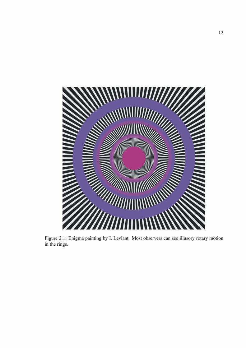
2.2 Stimulus & Methods

The racetrack stimulus is constructed in the following way: In the beginning N dots are

randomly and uniformly distributed in the annular region formed by two concentric circles.

Then a certain fraction c of the dots that are termed as the correlated dots are rotated by an

angle θ in the next frame and the remaining fraction of dots termed as the uncorrelated dots

have their positions randomly generated from a uniform distribution. The axis of rotation

is perpendicular to the plane of the annulus and passes through the center of the concentric

circles. The process continues and more and more frames are created. Depending on

how the correlated dots are selected from frame to frame different types of correlation are

possible. If M denotes the Markov transition probability matrix given by

M =

a b

c d

(2.1)

where a = Probability that a dot is correlated in present frame given that it was correlated

in the previous frame, b = Probability that a dot is uncorrelated in present frame given that

it was correlated in the previous frame, c = Probability that a dot is correlated in present

frame given that it was uncorrelated in the previous frame, d = Probability that a dot is

uncorrelated in present frame given that it was uncorrelated in the previous frame, then 3

special cases are as follows:

• Trajectory: In this case the correlated dots are fixed and so they trace out a circular

15

trajectory as they move.

M =

1 0

0 1

(2.2)

• Memoryless: In this case correlated dots are selected randomly and uniformly inde-

pendently of what happened in the past.

M =

c 1− c

c 1− c

(2.3)

where c =(no. of correlated dots/total no. of dots) is the dot correlation.

• Memory: In this case if a dot was correlated in the previous frame it will not be

correlated in the present frame.

M =

0 1

c1−c

1− c1−c

(2.4)

Note that c ∈ [0, 0.5] in this case. Unless otherwise stated this is the type of cor-

relation that will be used throughout the experiments. It completely eliminates the

appearance of “multiple dot trajectories” in which some dots would be recognized as

moving along an extended trajectory in the presence of noise. Algorithm 1 summa-

rizes the procedure for generating racetrack frames using this type of correlation.

The time interval for which a frame stays on screen is termed as the frame duration

fd. The magnitude of θ is fixed at 5◦ (this corresponds to an angle of approximately 20’

on the eye in our experiments) and the sign of θ determines the direction in which the

correlated dots move (clockwise or anticlockwise). The sign of θ is randomly changed in

16

Algorithm 1: Racetrack

Frame 0: Randomly generate N dots uniformly distributed in the annular region1

formed by two concentric circles. Partition the dots into two sets A and B. Set A←

{all N dots}. Set B← empty set.

Set C← {choose c*N dots from set A}. Set D← A−C+B2

Rotate dots in set C by θ. Update positions of dots in set D by randomly generating3

them again such that they are within the annular region. The dots in C and D give the

next frame.

Set A← Set D. Set B← Set C.4

Goto step 2 to create the next frame.5

time according to following process: Starting at time t = 0, a coin is tossed in intervals of

Ttoss = 3s. The sign of θ is positive if the coin comes heads up and negative if the coin

comes up tails.

The racetrack stimulus is shown to an observer and the observer is asked to enter via the

two mouse buttons whether he or she sees motion in clockwise or anticlockwise direction.

Figure 2.2 shows a few frames (resized to fit on the page) of the racetrack for c = 0.5, dot

density = 5 dots per square degree at the eye, the angle subtended by the outer circle diam-

eter at the eye during experiment = 10◦, the angle subtended by the inner circle diameter

at the eye during experiment = 7◦. The racetrack dots are black and a grey background (a

grey value of 150 on a scale of 0 black to 255 white) is used throughout our experiments.

17

Figure 2.2: A few frames of the racetrack stimulus (resized to fit on page).

All experiments are done using a CRT monitor. The angle subtended by the outer circle

diameter at the eye is fixed at 10◦ in all the experiments.

Figure 2.3(a) shows two curves - the dotted curve represents the input function which

is generated by the coin toss process described earlier. It tells the direction in which the

correlated dots in the stimulus are moving. The solid curve is the response curve and tells

the direction in which motion is perceived by the observer. Because c = 0.5 is a case of very

strong correlation, the observer is able to follow the motion in the stimulus very accurately

and therefore the response curve closely matches the input curve but is time-shifted by

the reaction time of the observer - the amount of time it takes for the brain to process

the motion signal and the observer to press the mouse button. Figure 2.3(b) shows the

18

0 10 20 30 40 50 60−2

0

2

Time (s)

Mot

ion

motion generated by computermotion reported by observer

0 1 2 3 40

0.5

1

time delay (s)

Cro

ss C

orre

latio

n fn

.

τ

χ

Figure 2.3: (a) The dotted curve is the motion generated by the computer and the solidcurve is the motion reported by the observer. (b) normalized cross correlation function ofthe two curves in (a). χ is the maximum value of the normalized cross correlation functionand τ is the time delay at which χ occurs.

19

cross-correlation function of the input and response curves1 . Define χ to be the maximum

cross-correlation and τ to be the time delay at which the maximum cross-correlation occurs

- τ is the amount of time by which the response curve has to be left shifted in Figure 2.3(a)

such that it matches best with the input curve. Thus χ is a measure of how well the observer

is able to follow the embedded motion in the stimulus and τ represents the total reaction

time of the observer.

Most of the experiments on visual motion in the past have employed displays whose

duration is only a fraction of a second to about 2s or so; the motion occurs in only one di-

rection for the duration of the display. This is in contrast to the racetrack which is shown to

an observer for duration of about 60s in a trial. Previous experiments characterize the per-

formance of an observer by measuring the fraction of trials in which the observer correctly

detects the direction of motion. On the other hand in the racetrack the direction of motion

keeps on changing randomly in time and the performance of an observer is characterized

by the χ measure described above. Multiple trials are taken and averaged to obtain a mean

value of the χ measure.

All expriments were done after approval from Committee for Protection of Human

Subjects (CPHS) UC Berkeley.

1Mathematically, the normalized cross correlation of two curves x(t) and y(t) is given by z(t) where

z(t) =

∫ +∞−∞ x(u)y(u + t)du(∫ +∞

−∞ x2(u)du ·∫ +∞−∞ y2(u)du

)1/2

20

2.3 Effect of dot correlation, frame duration, dot density

and annulus size on χ and τ

Our first experiment was to study the effect of four parameters on χ and τ : the dot

correlation c which is the fraction of dots correlated in the racetrack, the frame duration

fd which is the length of time a frame stays on screen, the dot density dd and the angle

subtended by inner circle at the eye ic. In all experiments the angle subtended by the outer

circle at the eye is fixed at 10◦. Experiments were done with 4 observers. In all trials the

observers had only two choices - clockwise motion indicated by right mouse button click

and anticlockwise motion indicated by left mouse button click. No option was given to

indicate no motion.

2.3.1 Effect of dot correlation c

Figure 2.4(a) shows the plot of χ vs. c for ic = 7◦. The χ values have been split into

two groups: one group having fd = {10, 30, 50} ms and the other group having fd =

{80, 100} ms. The data over different dot densities has been averaged to get the curves in

figure 2.4 as the dot density does not make any difference in χ values (ref. section 2.3.3).

Each circle or cross in figure 2.4 represents the mean value of χ over a large number of

trials and the length of error bar is equal to 1 standard deviation. At c = 0, there are no

correlated dots and the input curve does not have any physical significance. The χ value at

c = 0 however does not average out to be zero because χ is the maximum cross-correlation

21

between input and response curves. From the graph it is seen that at ic = 7◦, χ vs. c seems

to be having an exponentially rising profile. At high values of c, χ approaches its maximum

possible value of 1 representing perfect detection of the embedded motion in the stimulus.

The performance is better for fd = {10, 30, 50} ms than for fd = {80, 100} ms. Figure

2.4(b) shows the plot of χ vs. c for ic = 9.5◦ together with 1 sigma error bars. At ic = 9.5◦

the annulus becomes very narrow and the dots seem to be moving in a 1 dimensional strip

instead of a 2D annulus. The increase in χ with c is natural as c directly underscores the

amount of motion embedded in the stimulus.

2.3.2 Effect of frame duration fd

Figure 2.5 shows χ vs. fd curve at c = 0.1, dd = 5, ic = 7◦. It is found that fd ∼ 30

ms is optimal for motion perception. The perception of motion is critically dependent

on the frame duration used. The same sequence of frames that evoke perception of vivid

motion at fd = 30 ms fail to evoke any perception of motion whatsoever at fd � 200

ms (ref. the decrease in χ in figure 2.5 as fd is increased). As explained in later chapters

this is because the motion computed by local motion detectors at time t is based on the

spatiotemporal signal from time t − T to time t where T ∼ 200 ms is the temporal size

of receptive fields of motion sensitive cells found in area V1/MT of the brain, so when

fd � T the spatiotemporal signal is mostly constant within a bin of duration T and local

motion detectors will fail to register motion.

22

0 0.1 0.2 0.3 0.4 0.50

0.2

0.4

0.6

0.8

1

χ

dot correlation

fd ∈ {10,30,50} msfd ∈ {80,100} ms

(a)

0 0.1 0.2 0.3 0.4 0.50

0.2

0.4

0.6

0.8

1

χ

dot correlation

fd ∈ {10,30,50} msfd ∈ {80,100} ms

(b)

Figure 2.4: (a) Variation of χ with c for ic = 7◦. (b) Variation of χ with c for ic = 9.5◦.

23

0 20 40 60 80 1000

0.2

0.4

0.6

0.8

1

frame duration (ms)

χ

Figure 2.5: χ vs. frame duration fd. c = 0.1, dd = 5, ic = 7◦. fd ∼ 30ms is found to beoptimal for motion perception.

24

0 5 10 15 20 250

0.2

0.4

0.6

0.8

1

dot density (dots/degree2)

χ

Figure 2.6: χ vs. dot density dd. c = 0.2, fd = 30ms, ic = 7◦. Observer performance doesnot depend on dot density.

2.3.3 Effect of dot density dd

Figure 2.6 shows the variation of χ with the dot density at c = 0.2, fd = 30ms, ic = 7◦.

As can be seen human observers are remarkably insensitive to the dot density in the display.

This means it is the relative proportion of correlated dots that matters not their absolute

number. In the next chapter it will be shown that this finding immediately rules out motion

models based on matching features to their nearest neighbors in the next frame.

25

0 2 4 6 8 100

0.2

0.4

0.6

0.8

1

inner circle diameter (degrees)

χ

Figure 2.7: Plot of χ vs. ic for c = 0.1, dd = 5, fd = 30 ms.

2.3.4 Effect of angle subtended by inner circle ic

Figure 2.7 shows χ vs. ic, the angle subtended by inner circle diameter at the eye. The

angle subtended by the outer circle diameter is held fixed at 10◦. It is found that changing

ic from 1◦ to 7◦ has little effect on χ but increasing ic further leads to significant drop in

χ. At ic = 9.5◦ the annulus becomes very narrow and the dots seem to be moving in a 1D

ring instead of a 2D annulus.

26

0 0.2 0.4 0.6 0.8 1

0.5

1

1.5

2

2.5

3

3.5

χ

τ (s

)observer1observer2observer3observer4

Figure 2.8: Scatter plot of τ vs. χ for 4 observers together with a piecewise linearized fit.At high χ, τ is around 0.5s with little variation. As χ decreases τ as well as its variationincrease.

2.3.5 Effect on the reaction time τ

Figure 2.8 shows a scatter plot of τ vs. χ together with a piecewise linearized fit ob-

tained by averaging the data. For high values of χ such as χ > 0.9 when the motion is very

clear to an observer, τ is around 0.5s with a small variation. At the other extreme when

χ is small and it is difficult to discern the motion τ jumps to around 2.5-3s with a large

variation. The parameters that tend to increase χ, tend to decrease τ and vice-versa. As an

example Figure 2.9 shows the variation of τ with c.

27

0 0.1 0.2 0.3 0.4 0.50

0.5

1

1.5

2

dot correlation

τ (s

)

fd = {10, 30, 50} msfd = {80, 100} ms

Figure 2.9: Plot of τ vs. c at ic = 7◦

28

2.4 The Omega Effect and reproducibility of observer re-

sponse

The zero dot correlation (c = 0) is a special case of the racetrack stimulus. At c = 0 all

the dot pattern frames are randomly generated and there is no embedded correlation. Some

observers report seeing motion whereas others report the impression of what Newsome

& Pare, 1988 call as “twinkling visual noise” with no net motion in any direction. A

large percentage of the observers have remarked that after prolonged gazing the motion

becomes more or less voluntary — it is possible to will it in either direction and typically

it goes in one direction for 1/4 to 1/2 of the full circle and then reverses direction and

keeps oscillating. Some observers also remark that at times motion in both clockwise and

anticlockwise directions is seen simultaneously in different portions of the racetrack — this

is especially more pronounced for the ic = 9.5◦ case than for ic = 7◦. A few observers

also report that the motion switches direction when the mouse key is pressed.

(Rose & Blake, 1998) have investigated this special case of c = 0 before and termed the

perception of rotary motion at c = 0 as the “omega effect”. It has the basic ingredients of a

bistable illusion: the display consists of random dots resulting in ambiguous motion signals

but observers report seeing rotary motion. However one characteristic of the omega effect

different from other bistable illusions is that in the omega effect after prolonged viewing an

observer can usually instantaneously will the direction of motion to be either CW or CCW

whereas in other bistable illusions such as the necker cube it takes a few seconds for an

29

observer to will a change in percept.

This section takes a closer look at the c = 0 case of the racetrack. It is found that an

important characteristic of the “omega effect” is that at c = 0 the same stimulus movie

produces different responses from an observer in different trials. The reproducibility of

an observer’s response to a stimulus can be quantified in the following way: an observer

is shown the same stimulus in n trials that results in n response curves e.g. figure 2.10

shows the result of showing an observer the same stimulus in 6 trials. If two curves are

selected from the pool of n response curves and cross correlated the maximum value of

the normalized cross correlation function2 represents the degree to which the two curves

are similar e.g. figure 2.11 shows the normalized cross correlation function of 1st and 2nd

response curves in figure 2.10. There are a total of nC2 combinations giving nC2 values of

maximum cross correlation. These values are averaged to get a measure of reproducibility

of an observer response that is denoted by ζ . Figure 2.12 plots the mean and sigma of ζ as a

function of dot correlation. Trials were also conducted in which the stimulus was different

from trial to trial. The ζ values obtained by cross correlating the response curves from these

trials give the noise level that we can expect to find in the computation of ζ corresponding

to zero reproducibility of response. We find that ζ noise mean = 0.112, ζ noise sigma =

0.145. From figure 2.12 it is seen that ζ at c = 0 is close to the noise level. Thus even

though people see rotary motion in the racetrack at c = 0, their responses do not depend on

what dot pattern is shown to them.

2a window of [-4,4]s is used

30

0 20 40 60 80 100 120−2

−1

0

1

2stimulususer response

0 20 40 60 80 100 120−2

−1

0

1

2

0 20 40 60 80 100 120−2

−1

0

1

2

0 20 40 60 80 100 120−2

−1

0

1

2

0 20 40 60 80 100 120−2

−1

0

1

2

0 20 40 60 80 100 120−2

−1

0

1

2

Figure 2.10: Response curves of an observer to the same stimulus in 6 trials (c = 0.03, dd =5, fd = 30 ms, ic = 7◦)

31

−3 −2 −1 0 1 2 3

0

0.2

0.4

0.6

0.8

1

time shift (s)

cros

s co

rrel

atio

n fn

.

ζ

Figure 2.11: Cross correlation function of first two response curves in Figure 2.10. ζ isdefined as maximum value of the cross correlation function

32

0 0.02 0.04 0.06 0.08 0.10

0.2

0.4

0.6

0.8

1

threshold

dot correlation

ζ

observer1observer2observer3observer4

Figure 2.12: Plot of ζ vs. c for 4 observers. fd = 30 ms, dd = 5, ic = 7◦.

33

(a)0 10 20 30 40

0

200

400

600

800

1000

1200

1400

Inter Flip Interval (s)

coun

t

(b)−2 0 2 4 60

0.1

0.2

0.3

0.4

0.5

0.6

0.7

ln(Inter Flip Interval)

pdf

Figure 2.13: (a) histogram of Inter Flip Interval (IFI) at c = 0. (b) normalised histogram ofln(IFI) together with a Gaussian fit (black curve).

Figure 2.13(a) shows the histogram of the inter flip interval (IFI) which is the time

interval between spontaneous reversals in direction of motion at c = 0. The mode of the

histogram reflecting the most frequently occuring value of IFI occurs at IFI ∼ 2s. The

histogram is well approximated by a lognormal distribution meaning that if one were to

plot the histogram of the log of IFI that histogram would be normally distributed. This is

shown in figure 2.13(b) which plots the pdf (probability density function) of ln(IFI) together

with a Gaussian fit. As can be seen the Gaussian curve fits the experimental data extremely

well. The lognormal distribution (Limpert, Stahel, & Abbt, 2001) is a commonly occuring

distribution for quantities that have a one-sided range of the form (a, +∞) where a is finite

e.g. for IFI a = 0. The IFI of many bistable illusions is lognormally distributed. (Riani &

Simonotto, 1994) write “such distributions are common in biology and can be interpreted

in terms of the noise driven motion of a state point which randomly crosses a threshold or

surmounts an energy barrier.”

34

Parameters Just detectable threshold cfd = {10, 30, 50} ms ic = 7◦ 0.02 – 0.04

fd = {10, 30, 50} ms ic = 9.5◦ 0.07 – 0.13fd = {80, 100} ms ic = 7◦ 0.04 – 0.11

fd = {80, 100} ms ic = 9.5◦ 0.09 – 0.20

Table 2.1: Minimum dot correlation required for motion to be just detectable by a human(from data on 4 observers).

2.5 Thresholds on motion perception

Figure 2.12 can also be used to determine what is the minimum fraction of dots that have

to be correlated so that the motion in racetrack is just detectable by a human. Empirically

the threshold can be defined as the dot correlation to be the value at which ζ is equal to ζ

noise mean + ζ noise sigma i.e. it is the value of c at which observer responses start showing

some reproducibility. This threshold is plotted in Figure 2.12 and using this criterion the

threshold c is found to lie in the range 0.03 to 0.065 for the 4 observers at fd = 30 ms,

ic = 7◦.

Another possible way to determine the threshold correlation is to use the χ vs. c curve.

The threshold correlation can be defined as the value of c for which χ is equal to mean(χ) +

σ(χ) at c = 0. Using this criterion, the threshold values of c for 4 observers are summarized

in table 2.1.

This range of threshold seems to compare favorably with other studies such as those

of Newsome & Pare, 1988; Newsome, Britten, & Movshon, 1989 which report a threshold

c of 2–6%. Newsome & Pare, 1988; Newsome et al., 1989 have done their experiments

on monkeys, the stimulus consists of translational stochastic motion that is shown to the

35

monkey for 2 sec and then the monkey has to decide whether the motion was upward or

downward, their operating definition to compute the threshold is very different from the

way I determine the threshold. Taking all these differences into account there seems to be a

good qualitative match between the threshold reported here and that reported by Newsome

et al.

2.6 Can an observer tell apart c = 0 from c = 0.1?

While taking data of previous experiments I noticed that the stimulus at c = 0.1 looks

just as random as the stimulus at c = 0 and was therefore surprised to find a high value

of χ for the trial at c = 0.1. In order to investigate this systematically another series

of experiments were done in which an observer was shown a stimulus whose parameters

were randomly selected from following values: dd = {1.4, 5, 10} dots per sq. deg., fd =

{10, 30, 50} ms , c = {0, 0.1}. The ic was fixed at 7◦. At the end of the trial the observer

was asked if he/she thought that the dot pattern was (a) completely random or (b) there

was some correlation embedded in the dots. This amounted to classifying the stimulus as

c = 0 or c = 0.1 respectively. The duration of the trials was at least 60s with mean duration

around 100s. The test was done on 4 observers and the data is summarized in table 2.2.

The meaning of the various entries in table 2.2 is as follows e.g. observer 1 took a total

of 54 trials. The normalized confusion matrix is given by a00 a01

a10 a11

where

36

Observer total Confusion Matrix mean(χ) sigma(χ)

1 54(

30/31 1/317/23 16/23

)=

(0.97 0.030.30 0.70

) (0.09 0.290.78 0.74

) (0.12 N/A0.12 0.11

)2 27

(8/13 5/137/14 7/14

)=

(0.62 0.380.50 0.50

) (0.09 0.110.41 0.48

) (0.07 0.060.13 0.10

)3 23

(5/7 2/79/16 7/16

)=

(0.71 0.290.56 0.44

) (0.10 0.010.52 0.54

) (0.07 0.140.20 0.12

)4 13

(6/10 4/100/3 3/3

)=

(0.60 0.400 1

) (0.15 0.25N/A 0.68

) (0.09 0.09N/A 0.13

)Table 2.2: A test in which observers are asked to classify whether or not the racetrack hasany embedded correlation in it.

a00 = number of c = 0 trials correctly classified as c = 0 ÷ total number of c = 0 trials

a01 = number of c = 0 trials incorrectly classified as c = 0.1 ÷ total number of c = 0 trials

a10 = number of c = 0.1 trials incorrectly classified as c = 0 ÷ total number of c = 0.1

trials

a11 = number of c = 0.1 trials correctly classified as c = 0.1 ÷ total number of c = 0.1

trials

The off diagonal entries of the matrix correspond to the so called Type I and Type II errors.

The mean and sigma of χ values corresponding to the different cases also shown in table 2.2

The large values of Type I and Type II errors means that observers are unable to subjectively

distinguish between c = 0 and c = 0.1. The high values of χ for misclassified c = 0.1 trials

on the other hand imply that observers are nevertheless able to detect the dot correlations

in c = 0.1 trials to an impressive degree of accuracy. This is a most surprising result found

in the experiments so far.

37

Figure 2.14: A frame in which only a 60◦ sector of the racetrack is made visible.

2.7 What happens if only a sector of the complete race-

track is made visible?

The next experiment was to take trials in which an observer was shown only a sector

of the racetrack instead of the full 360◦ annulus. The sector was positioned at the top of

the screen and was symmetrical about the vertical. Figure 2.14 shows a frame when a 60◦

sector is made visible. The data was taken on the same 4 observers of section 2.3. All the

trials were done with ic = 7◦.

Figure 2.15 shows χ averaged over observers vs. c for ic = 7◦ when only a partial

sector of the racetrack is made visible to the observer. The sector angle is varied from 10◦

to 360◦ (full racetrack visible at 360). 1 sigma error bars are also shown. It is seen that χ

drops off as the sector visible to the observer decreases. As the sector size is decreased the

amount of correlated dots visible decreases but so does the amount of noise dots i.e. the dot

38

0 0.1 0.2 0.3 0.4 0.50

0.2

0.4

0.6

0.8

1

dot correlation

χ

360°90°30°15°10°

Figure 2.15: Plot of χ vs. c when only a sector of the racetrack is made visible.

39

correlation c remains unchanged. The observer performance nevertheless drops showing

the important role that geometry plays in the detection of rotary motion. It seems that it is

advantageous to have motion cues all over the field of view. The next section probes this in

further detail.

2.8 Non-uniformly vs. Uniformly distributed motion cues

The results of previous section suggest that it seems if motion cues are localized to one

part of the annulus, the system does not perform as well. In order to probe this further

a modified racetrack was designed in which the correlated dots are concentrated within a

sector of the annulus instead of being distributed uniformly throughout the annulus. The

algorithm used to generate the frames is summarized in algorithm 2. While selecting the

dots to be correlated, algorithm 2 gives preference to dots that lie within a sector of the

racetrack. Comparing algorithm 1 and 2 the total number of correlated dots is the same

in the two cases but the correlated dots are concentrated in the sector for algorithm 2 and

are uniformly distributed throughout the annulus for algorithm 1. Note that there will

in general be correlated dots that lie outside the sector when using algorithm 2. With

reference to algorithm 2, the fraction of correlated dots that lie outside the sector is given

by f = max(0, 1− |As|/cN) 3. f can be computed for each frame of the racetrack. Ideally,

we would like f to be zero — this corresponds to the case when all the correlated dots are

localized within the sector. Figure 2.16 shows the mean and sigma of f simulated by a

3|A| denotes cardinality of set A

40

0 0.1 0.2 0.3 0.4 0.50

0.2

0.4

0.6

0.8

1

dot correlation

f 10°15°30°60°90°

Figure 2.16: Plot showing fraction of correlated dots that lie outside the sector using themodified racetrack algorithm

large number of trials. As an example when the sector angle is 60◦ we find f is close to

zero for c = 0 to 0.1 With further increase in c, f increases and at c = 0.5 mean(f ) = 0.833.

If the correlated dots were evenly distributed throughout the annulus, then the fraction of

correlated dots lying outside the sector would be around (360−60)/360 = 0.833. This is

in fact same as the mean value of f at c = 0.5 which means that at c = 0.5 the stimulus

generated using algorithm 2 is similar to the stimulus that is obtained using the normal

racetrack algorithm.

An experiment was done in which the stimulus was generated using algorithm 2 and

the sector angle was set to 60◦. The dd, ic, fd were set to 5 dots per sq. degree, 7◦, 30ms

41

Algorithm 2: Modified Racetrack with correlated dots concentrated in a sector in-

stead of being uniformly distributed throughout the annulus

Frame 0: Randomly generate N dots uniformly distributed in the annular region1

formed by two concentric circles. Partition the dots into two sets A and B. Set A←

{all N dots}. Set B← empty set.

Partition A into complementary sets: Set As ← {dots in set A that are in the sector}2

Set A′s ← {dots in set A that are not in the sector}

if cN <= |As| then3

Set C← {choose cN dots from set As}4

else5

Set C← {As + choose (cN−|As|) dots from A′s }6

Set D← A−C+B7

Rotate dots in set C by θ. Update positions of dots in set D by randomly generating8

them again such that they are within the annular region. The dots in C and D give the

next frame.

Set A← Set D. Set B← Set C.9

Goto step 2 to create the next frame.10

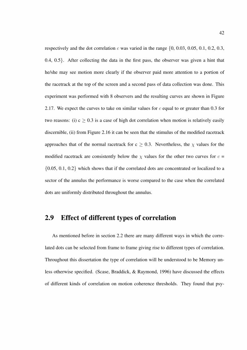
42

respectively and the dot correlation c was varied in the range {0, 0.03, 0.05, 0.1, 0.2, 0.3,

0.4, 0.5}. After collecting the data in the first pass, the observer was given a hint that

he/she may see motion more clearly if the observer paid more attention to a portion of

the racetrack at the top of the screen and a second pass of data collection was done. This

experiment was performed with 8 observers and the resulting curves are shown in Figure

2.17. We expect the curves to take on similar values for c equal to or greater than 0.3 for

two reasons: (i) c ≥ 0.3 is a case of high dot correlation when motion is relatively easily

discernible, (ii) from Figure 2.16 it can be seen that the stimulus of the modified racetrack

approaches that of the normal racetrack for c ≥ 0.3. Nevertheless, the χ values for the

modified racetrack are consistently below the χ values for the other two curves for c =

{0.05, 0.1, 0.2} which shows that if the correlated dots are concentrated or localized to a

sector of the annulus the performance is worse compared to the case when the correlated

dots are uniformly distributed throughout the annulus.

2.9 Effect of different types of correlation

As mentioned before in section 2.2 there are many different ways in which the corre-

lated dots can be selected from frame to frame giving rise to different types of correlation.

Throughout this dissertation the type of correlation will be understood to be Memory un-

less otherwise specified. (Scase, Braddick, & Raymond, 1996) have discussed the effects

of different kinds of correlation on motion coherence thresholds. They found that psy-

43

0 0.1 0.2 0.3 0.4 0.50

0.2

0.4

0.6

0.8

1

dot correlation

χ

normal racetrackmodified racetrack; before hintmodified racetrack; after hint

Figure 2.17: χ vs. c for three cases (i) normal racetrack, (ii) modified racetrack, (iii)modified racetrack and the observers are given a hint that they may see motion more clearlyif they pay more attention to a sector of the racetrack

44

0 0.02 0.04 0.06 0.08 0.10

0.2

0.4

0.6

0.8

1

dot correlation

χtrajectorymemory

Figure 2.18: Effect of type of correlation used on observer performance.

chophysical results were not much affected by the choice of correlation for the kinds of

correlation used in their experiments. Figure 2.18 shows the results of my experiments

in which the dots could be correlated according to trajectory or memory. It is found that

when the observer is unaware of the trajectory his/her performance is same as in the mem-

ory case. However, if the observer becomes aware that the correlated dots are moving in

a trajectory s/he can significantly increase his/her performance by paying attention to the

correlated dots and tracking the trajectory.

45

2.10 Conclusion

This chapter described the racetrack stimulus and the associated experiments used to

gather quantitative psychophysical data characterizing visual motion perception. Observer

performance was investigated with respect to 4 parameters — the dot correlation c, frame

duration fd, angle subtended by inner circle diameter ic, and the dot density dd. The

dot correlation and frame duration are found to play important roles in the perception of

motion whereas the dot density is a weak parameter and does not have any appreciable

effect on the performance as long as the dot density is not extremely low (less than 10

dots) or extremely high (complete annulus is filled with dots and becomes black). The

case of zero dot correlation (c = 0) is a special case of the racetrack in which the dot

pattern is completely random and there is no deliberately embedded correlation. It has been

demonstrated that even though the c = 0 case evokes a perception of rotary motion — the

so called “omega effect”, the observer response does not depend on what dot pattern was

shown. However the “omega effect” does require a circular geometry and appropriate frame

duration. Empirical thresholds have been determined on the amount of dot correlation

required so that an observer is just able to detect the embedded motion. A surprising finding

is that observers are unable to subjectively distinguish c = 0 case from a case of weak

dot correlation such as c = 0.1 but they are subconsciously able to follow the embedded

motion at c = 0.1 to an impressive degree of accuracy. The performance of an observer

deteriorates if only a sector of the racetrack is shown instead of the complete annulus. Also

if the correlated dots are concentrated to within a sector of the annulus instead of being

46

uniformly distributed throughout the annulus the performance drops.

The next chapters will be devoted to developing models that can explain the experimen-

tal findings.

47

Chapter 3

Modeling visual motion perception:

Motion Correspondence vs. a

Correspondenceless model

3.1 Introduction

This chapter addresses the problem of developing a model that can successfully explain

the experimental psychophysics results of the previous chapter. Two models for this pur-

pose are discussed. In both models it is assumed that the positions of the dots are known.

The first model is based on matching a dot to its nearest neighbor (NN) in the next frame.

The pairs of matched dots generate 2 dot apparent motion cues from which rotary motion

is extracted. In the second model each dot is matched with every dot falling within a small

48

neighborhood in the next frame and the dot tends to move in the net direction. Both mod-

els employ a spatial distance weighting function which mimics the spatial receptive field

(RF) of a motion sensitive cell. The weighting function gives more weight to matches in

which the dots are close and less weight to matches in which dots are separated by a large

distance.

It is found that the model based on 2-dot motion correspondence cannot explain the

experimentally observed independence of observer performance on the dot density in the

display whereas the multi-dot correspondence model is able to explain this independence

in addition to other effects. The chapter also addresses the mechanisms responsible for

the delicate effects of frame duration on motion perception, the experimentally observed

position invariance of MST(d) cells and the omega effect in which a sequence of random

dot patterns evokes rotary motion perception.

3.2 Model Description

The input to both models is the dot positions in various frames.

3.2.1 Nearest Neighbor (NN) Model

This model takes the view that the basic problem required to be solved is the so called

motion correspondence problem — to figure out where each dot went in the next frame

(Dawson, 1991). When all the features in the display are identical and possess no dis-

49

tinguishing features such as in case of the racetrack, it has been argued that the optimal

matching should be such that the sum of path lengths is minimized (Ullman, 1979). The

path length of a pair is the separation distance. I do not suppose that the human visual sys-

tem goes through the process of systematically finding the optimal matching from frame

to frame in real time. The nearest neighbor (NN) model described here employs a greedy

algorithm that attempts to solve the correspondence problem by randomly selecting a dot in

the current frame, matching it to its nearest neighbor (NN) in the next frame and repeating

until all dots are matched subject to the constraint that every dot is given a unique match in

the next frame i.e. element integrity (Dawson, 1991) is preserved and many-one mappings

in which multiple dots of the current frame match to the same dot in the next frame are not

allowed. Figure 3.1(a) shows two successive racetrack frames superimposed on each other.

The dots in the current frame are colored red and the dots in the next frame are colored

blue. The lines in figure 3.1(b) indicate the pairings determined by the NN model. In my

implementation I do not go through the task of finding a corresponding dot for every dot in

the current frame — when the number of dots in the display is high the correspondences

of only a certain fraction of the dots are computed. This is done to: 1) speed up processing

time, 2) Because of the element integrity constraint as time progresses the matches com-

puted tend to have large separation distances/path lengths. These are spurious matches that

are later discounted by the spatial distance weighting function (w in eqn. 3.1). Limiting

the number of dots for which correspondences are computed avoids these spurious matches

which would be of no use anyway.

50

After computation of correspondences the next step in the model is to extract a 2 frame

rotary motion signal. This is achieved in the following way: the Nearest Neighbor matching

gives 2 dot apparent local motion cues. By taking the cross product with the radial vector

the 2 dot local motion cues can be converted into rotary motion signal. The 2 frame rotary

motion signal denoted by e is given by

e =

∑i(ri × vi)w(|~vi|)∑

i w(|~vi|)(3.1)

The summation is over the dots, ~ri is vector from the center relative to which rotary motion

is computed to dot i, ~vi are vectors obtained after NN matching (the lines in figure 3.1(b)),

and

w(x) =

1 |x| ≤ 0.5◦

max(0, 1− |x|−0.51.4−0.5

) |x| > 0.5◦

(3.2)

mimics the spatial profile of RF of a neuron1.

Figure 3.3(a) shows the two frame rotary motion signal e calculated using equation 3.1

for following parameters: c = 0.1, dd = 2.5dots/deg2, ic = 7◦, fd = 30ms. The signal

is positive for counter clockwise motion (CCW) and negative for clockwise motion (CW).

e(n) is computed as per equation 3.1 based on the NN matching between frame n− 1 and

frame n. To avoid cumbersome notation the dependence of e, r, v on time is implicit in

equation 3.1. e can either be viewed as a discrete time signal with sampling period fd

1from (Snowden, 1994) p. 57 “(Albright & Desimone, 1987) measured the receptive field (RF) size ofover 500 single cells in MT out to 25◦ eccentricity and found an approximate relationship of RF size =1.04◦ + 0.61eccentricity with a scatter of RF size that was approximately one-third of the RF size. Asmentioned above the field size of MT cells is approximately 10 times the equivalent of its V1 counterpart.However, if one only includes the direction selective cells of V1 then this figure reduces to only three times”.Also see e.g. (DeAngelis et al., 1993) p. 1100 for other physiological RF size measurements.

51

seconds or as a continuous time signal which is piecewise constant and changes in steps of

fd seconds.

The two frame rotary motion signal e is computed by taking just two successive frames

into consideration and is thus a differential motion signal which is very noisy with high

fluctuations. The human visual system must integrate information over a certain interval

of time to compute a reliable estimate of motion. In order to achieve this, the signal e

is passed through a moving averages filter whose purpose is to combine information over

time, to smooth out e and remove the high frequency noisy fluctuations in e. The resulting

signal denoted by I is shown in figure 3.3(b) and computed according to following equation

I(t) = e(t) ∗ g(t) (3.3)

The ∗ indicates convolution and g(t) is given by

g(t) =

1/T 0 ≤ t ≤ T

0 otherwise

(3.4)

T is the time interval over which the human visual system is believed to integrate motion

information. I choose T = 0.5s consistent with values of temporal integration window

reported e.g. in (Grzywacz et al., 1995).

While doing psychophysical experiments with human observers the only information

available is the direction in which the observer is seeing motion. Therefore in order to com-

pare model response with experimental psychophysics the signal I needs to be converted

into judgements of CCW or CW motion which can then be compared with the judgements

given by human observers. To achieve this, the signal I is passed through a level crossing

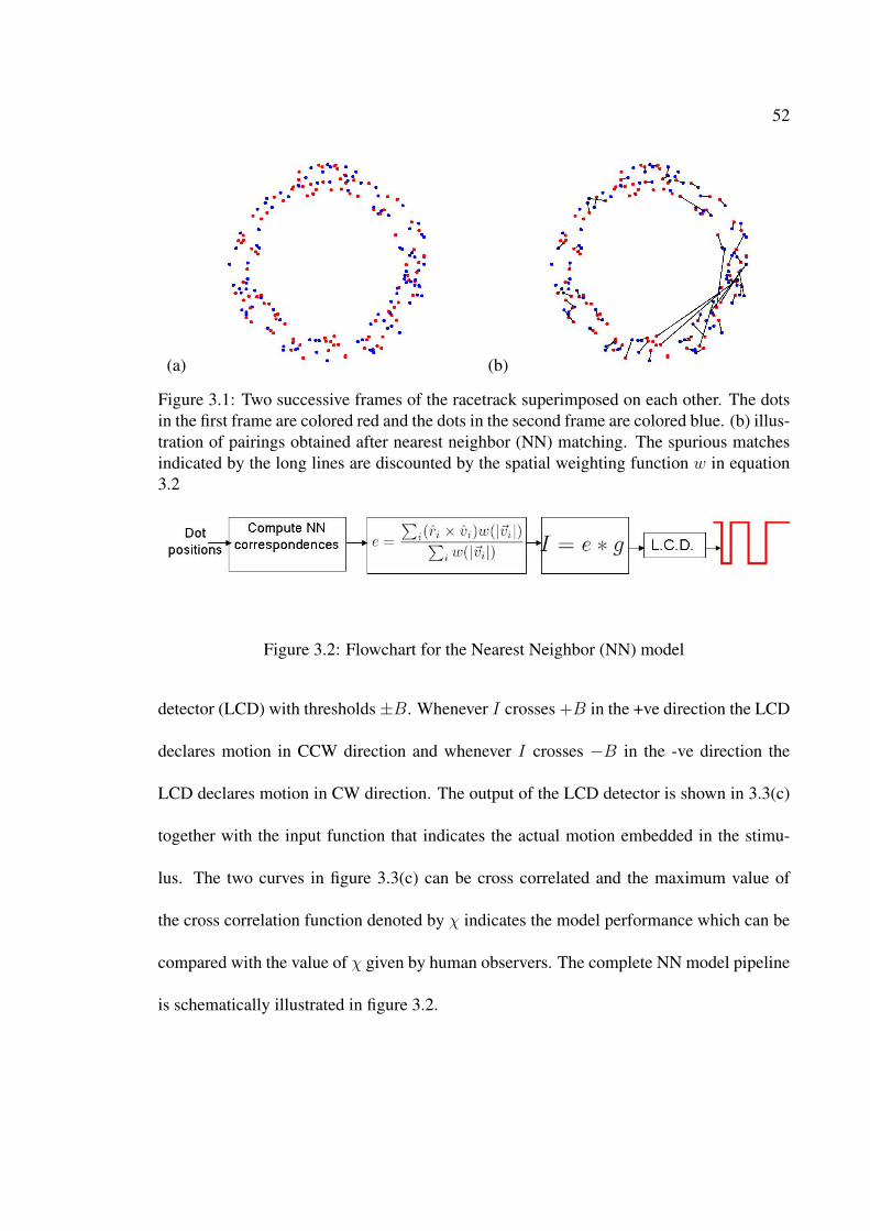
52

(a) (b)

Figure 3.1: Two successive frames of the racetrack superimposed on each other. The dotsin the first frame are colored red and the dots in the second frame are colored blue. (b) illus-tration of pairings obtained after nearest neighbor (NN) matching. The spurious matchesindicated by the long lines are discounted by the spatial weighting function w in equation3.2

Figure 3.2: Flowchart for the Nearest Neighbor (NN) model

detector (LCD) with thresholds±B. Whenever I crosses +B in the +ve direction the LCD

declares motion in CCW direction and whenever I crosses −B in the -ve direction the

LCD declares motion in CW direction. The output of the LCD detector is shown in 3.3(c)

together with the input function that indicates the actual motion embedded in the stimu-

lus. The two curves in figure 3.3(c) can be cross correlated and the maximum value of

the cross correlation function denoted by χ indicates the model performance which can be

compared with the value of χ given by human observers. The complete NN model pipeline

is schematically illustrated in figure 3.2.

53

0 20 40 60 80 100−0.5

0

0.5

Time (s)

e

0 20 40 60 80 100−0.1

0

0.1

Time (s)

I

0 20 40 60 80−1

0

1

Time (s)

mot

ion

inputmodel response

Figure 3.3: NN model response at c=0.1, fd=30ms, ic=7◦, dd=2.5 dots/deg2

54

3.2.2 Model2: a correspondenceless model

This model takes the view that since the dots are identical and have no distinguishing

features a dot in the present frame will match or be attracted to every dot in the next frame

and will tend to move in the net direction. The motion correspondence problem is bypassed.

The two frame motion signal e is computed as

e =

∑i

∑j(ri × vij)w(|vij|)√∑

i

∑j w(|vij|)

(3.5)

where ~vij is the vector from dot i in present frame to dot j in next frame. N is total number

of dots. The rest of the steps in model2 are identical to those in the NN model.

The following section compares the results of the two models with experimental psy-

chophysics.

3.3 Results

3.3.1 Effect of dot correlation c

Figure 3.4 shows χ vs. c curve for humans and the two models at dd = 5dots/deg2, ic =

7◦, fd = 30ms. Throughout the chapter length of errorbars is equal to 1 standard devia-

tion unless otherwise stated. Both models show an increase in χ with c. As c → 0.5 χ

approaches its maximum possible value of 1 implying perfect detection of the embedded

correlation. As mentioned before at c = 0 the input function does not have any physical

significance since there are no dots correlated according to the input function. The χ value

55

0 0.1 0.2 0.3 0.4 0.50

0.2

0.4

0.6

0.8

1

dot correlation

χ

experimentNN modelModel 2

Figure 3.4: χ vs. dot correlation c. Comparison of human and model performance.fd=30ms, ic=7◦, dd=5 dots/deg2. Throughout the chapter length of errorbars is equal to1 standard deviation unless otherwise stated. Although the NN model appears better, byaddition of suitable amount of noise the curve for Model2 can be made to fall to fit thepsychophysical data more closely.

at c = 0 is not zero since χ is the maximum value of the normalized cross correlation

function between input and observer/model response. The increase in χ with c is easy to

understand as the value of c directly underscores the amount of motion embedded in the

stimulus.

3.3.2 Effect of frame duration fd

Recall that the frame duration fd is defined as the length of time for which a frame

stays on screen. The length of time between disappearance of a frame and appearance of

56

next frame is negligible and can be taken to be zero. Figure 3.5 shows χ vs. fd curve for

humans and the models at c = 0.1, dd = 5dots/deg2, ic = 7◦. The behavior of the two

models is understood by following reasoning: the role of the moving averages filter is to

combine information over time and to remove the high frequency noisy fluctuations in e.

The time spacing between samples of e is given by the frame duration i.e. new information

arrives every fd seconds. The number of samples available in a time window T seconds is

thus T/fd. Therefore when fd is low there are more samples available and so the estimate

of the average computed by the moving averages filter is more accurate. Therefore as fd is

decreased the performance of the two models monotonically increases. For humans too we

see an increase in χ as fd is lowered from 100ms to 30ms. At fd = 10 ms χ for humans

is however less than χ at fd = 30 ms. Could this be due to some information overload

experienced by human observers at fd = 10 ms? While viewing the display at fd = 10

ms one can readily note a change in the quality: the dots seem to move too rapidly, they are

not as dark as at fd = 30 ms, appear washed out and the dots from multiple frames can be

seen simultaneously on the screen2.

3.3.3 Effect of annulus width

The angle subtended by the inner circle diameter at the eye is denoted by ic. Figure

3.6 shows χ vs. ic. The angle subtended by the outer circle diameter is held fixed at

10◦ in all experiments. For the NN model it is found that χ decreases with decrease in

2cf. when a ceiling fan rotates the blades can no longer be distinguished and appear fuzzy or faded.

57

0 20 40 60 80 1000

0.2

0.4

0.6

0.8

1

frame duration (ms)

χ

experimentNN modelModel 2

Figure 3.5: χ vs. frame duration (fd). For human observers fd=30ms is about optimumwhereas the models show steady improvement in χ as fd is decreased. The decrease in χ forhumans at fd<30ms may be explained by humans experiencing an information overload.c=0.1, ic=7◦, dd=5 dots/deg2

58

annulus width. This is because the number of correspondence mismatches made by the

model increase with decrease in annulus width. A correspondence mismatch refers to the

phenomenon when the correspondence match found by the model is not the true correlated

partner that was embedded in the stimulus. Varying the annulus width leads to changes

in geometry e.g. at ic = 9.5◦ the annulus becomes very thin and is better described as a

1D ring rather than a 2D annulus. The separation distance between a correlated dot and its

partner in the next frame is rθ where r is distance of dot from the center and θ is the angle

by which it is rotated. Therefore as ic is decreased the correlated dots tend to have larger

separation distance than when ic is low. This causes more correspondence mismatches

because the NN may no longer be the correlated partner (refer section 3.3.5). For humans

we observe that changing ic from 1◦ to 7◦ has little effect on χ but increasing ic further

leads to a drop in χ. Model2 does not appear to be sensitive to changes in ic.

3.3.4 Effect of dot density dd

Figure 3.7 shows χ vs. dot density at c = 0.2, fd = 30ms, ic = 7◦. Humans are

remarkably insensitive to the dot density in the display. This means it is the relative pro-

portion of correlated dots that matters not their absolute number. The NN model shows a

decrease in χ with increase in dot density. This is because as the dot density is increased

there are more dots per unit area in the display and so the probability that the NN is not

the correlated partner increases. This probability known as the probability of mismatch

is given by pm = 1 − exp(−πh2dd) (Williams & Sekuler, 1984) where h is the hop size

59

0 2 4 6 80

0.2

0.4

0.6

0.8

1

inner circle diameter (degrees)

χ

experimentNN modelModel 2

Figure 3.6: χ vs. angle subtended by inner circle (ic). c=0.1, fd=30ms, dd=5 dots/deg2,angle subtended by outer circle fixed at 10◦.

60

— the displacement given to the correlated dot and dd is the dot density. Model2 on the

other hand is insensitive to dot density and in agreement with experimental psychophysics.

For comparison the figure also shows χ vs. c curves for a model that matches a dot to

nearest n neighbors with n = {2, 4, 8}. Even with n = 8 there is a drop in χ at dd = 25

which is absent in the experimental curve. The correlated dot has an average hop size of

h = 0.37◦. Average number of dots in a circle of radius h = πh2dd = 0.4301 × dd. At

dd = 25, 0.4301× dd ∼ 11 so on average we can expect to find about 11 noise dots in the

circle. Since n = 8 is less than 11 a drop occurs in χ. The experimental invariance of ob-

server performance to dot density in the display which is consistent with Model2 provides

strong evidence that all the dots falling within a small neighborhood are considered when

computing the local motion. Model2 is the limit as n→∞.

3.3.5 Effect of hop size h

The probability of mismatch formula predicts that in addition to dot density the NN

model should show a marked dependence on the hop size of the correlated dots. In all the

experiments up until now the correlated dots were rotated by an angle of 5◦. With ic = 7◦

and angle subtended by outer circle fixed at 10◦ this translates to average displacement of

7+104×5× π

180= 0.37◦ visual angle on the eye. Figure 3.8(a) shows the effect of varying the

hop size for the NN model. The correlated dots were rotated by angles of {1,5,10,15,20,25}

degrees corresponding to average displacements of {0.074, 0.37, 0.74, 1.11, 1.48, 1.85}

degrees visual angle on the eye. As predicted by the probability of mismatch formula the

61

0 5 10 15 20 250

0.2

0.4

0.6

0.8

1

dot density (dots/degree2)

χ experimentNN modelModel 2n=2n=4n=8

Figure 3.7: χ vs. dot density (dd). Human observers and model2 are insensitive to dotdensity whereas the NN model and its variants have a marked dependence on dot densityas dictated by the probability of mismatch (see text for details). c=0.2, fd=30ms, ic=7◦.

62

model performance decreases with increase in hop size. Different curves are obtained for

different dot densities. Since the probability of mismatch depends on both the hop size and

the dot density re-plotting the χ values in figure 3.8(a) against h√

dd instead of h collapses

the distinct curves in 3.8(a) into a single curve in 3.8(b). By contrast the corresponding data

for human observers is shown in figures 3.8(c)-(d). Human observers also show decrease

in χ with increase in hop size, but compared to NN model humans show opposite behavior:

χ vs. hop size for different dot densities does not give separate curves and plotting χ

against h√

dd separates out the curves. For humans the hop size at which failure occurs is

independent of dot density. These figures together with figure 3.7 highlight the limitation

of a correspondence based model and demonstrate that it cannot account for an important

aspect of experimental data namely independence of χ from dot density. Note from figure

3.8(c) that when hop size is increased the perception of motion disappears in the display

even though the dot correlation is very high (c = 0.4). This is because if the hop size

becomes greater than the RF size, motion sensitive neurons will fail to register motion.

Figure 3.8(e) shows χ vs. h and Figure 3.8(f) shows χ vs. h√

dd for model2. The curves are

similar to those for human observers and the hop size at which failure occurs is independent

of dot density. This is because model2 does not match a dot just to its NN but rather

to every dot in the next frame. In figures 3.8(a,e) χ is above zero level at hop size of

1.48◦ even though the weighting function w becomes zero at 1.4◦ as per equation 3.2.

The reason for this is that figures 3.8(a,e) only show the average displacement; when dots

are rotated by 20◦ the dots at the boundary of the inner circle undergo a displacement of

63

3.5× 20× π180

= 1.22◦ which is less than 1.4◦.

3.3.6 Model Sensitivity to center position

By definition of rotation, any measure of rotary motion has to be specified with respect

to some center of rotation (more accurately the axis of rotation has to be specified). In

equations (3.1, 3.5) the radial vector ~ri is from the center relative to which rotary motion

is computed to dot i in the frame. The axis of rotation is of course the line perpendicular

to the screen that passes through the center of rotation. In all the results presented uptil

now the center position used in the simulations was the true center of the racetrack. What

happens if the center position of the racetrack is not known? Figure 3.9 shows a schematic

in which point O is the true center relative to which the correlated dots are rotating and

point C is the center relative to which rotary motion is computed by the model. ~vi is a

motion cue. The rotary motion relative to the true center O is given by∑

i ~ri × ~vi whereas

the rotary motion relative to C is given by∑

i~r′i × ~vi. We have

S =∑

i

~r′i × ~vi

=∑

i

( ~CO + ~ri)× ~vi

=∑

i

~CO × ~vi +∑

i

~ri × ~vi

= ~CO ×∑

i

~vi +∑

i

~ri × ~vi

=∑

i

~ri × ~vi provided∑

i

~vi = 0

64

(a)0 0.5 1 1.5

0

0.2

0.4

0.6

0.8

1

Hop size (degrees)

χ

dd=1.3dd=5dd=10

(b)0 1 2 3 4 5

0

0.2

0.4

0.6

0.8

1

Hop size*sqrt(dd)

χ

dd=1.3dd=5dd=10

(c)0 0.5 1 1.5

0

0.2

0.4

0.6

0.8

1

Hop size (degrees)

χ

dd=1.3dd=5dd=10

(d)0 1 2 3 4 5

0

0.2

0.4

0.6

0.8

1

Hop size*sqrt(dd)

χ

dd=1.3dd=5dd=10

(e)0 0.5 1 1.5

0

0.2

0.4

0.6

0.8

1

Hop size (degrees)

χ

dd=1.3dd=5dd=10

(f)0 1 2 3 4 5

0

0.2

0.4

0.6

0.8

1

Hop size * sqrt(dd)

χ

dd=1.3dd=5dd=10

Figure 3.8: χ vs. hop size for various dot densities. c=0.4, fd=30ms, ic=7◦. (a,b) NN model(c,d) humans (e,f) Model2

65

The condition∑

i ~vi = 0 is true in case of the racetrack — the uncorrelated dots are uni-

formly distributed and generate motion cues in all directions with equal probability; the

correlated dots generate motion cues in tangential direction which when summed over the

entire 360◦ annulus add up to zero. The expected value of∑

i ~vi is thus zero. Therefore it

seems accurate knowledge of position of the true center relative to which rotation occurs is

not needed. Figure 3.10(a) shows model sensitivity to knowledge of true center position.

The rotary motion is computed by the models relative to a point C that is offset from the

true center O. The offset is given by ~OCRi

where Ri is radius of inner circle. It can be seen

that the χ values are not affected by uncertainty in knowledge of true center position. This

may explain the experimentally observed position invariance of MST(d) cells — the fact

that the cells are insensitive to where in their RF rotation occurs (Graziano et al., 1994).

It seems that when only a sector of the racetrack is made visible the condition∑

i ~vi = 0

may not hold true because of the correlated dots. However if two diametrically opposite

located sectors are displayed then∑

i ~vi = 0. Figure 3.10(b) shows χ vs. offset for the

two cases — type1 when only a single 90◦ sector is made visible and type2 when two

diametrically opposite located sectors each 45◦ in size are displayed. Interestingly both

models are robust enough to the offset even when only a sector of the racetrack is displayed

irrespective of whether it is type1 or type2.

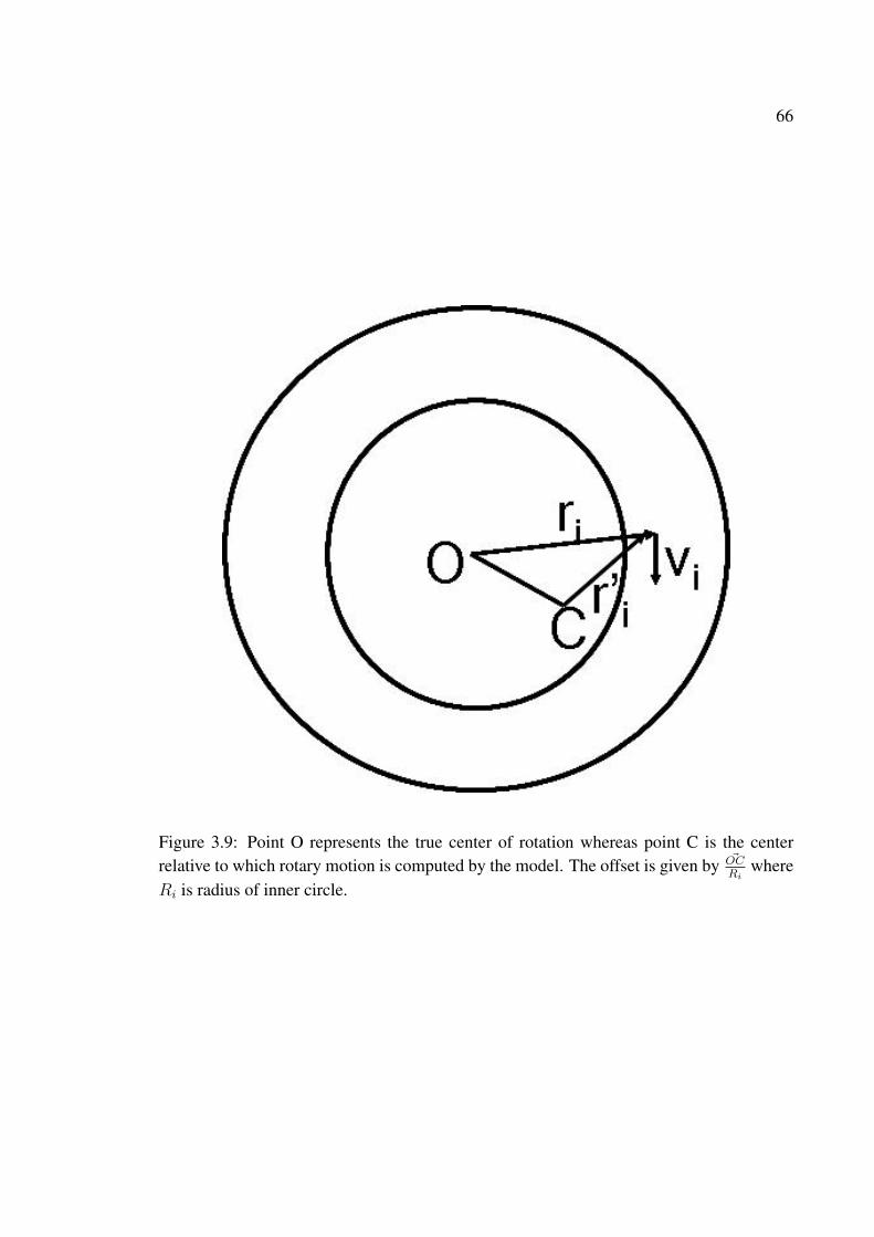
66

Figure 3.9: Point O represents the true center of rotation whereas point C is the centerrelative to which rotary motion is computed by the model. The offset is given by ~OC

Riwhere

Ri is radius of inner circle.

67

(a)0 0.2 0.4 0.6 0.8

0

0.2

0.4

0.6

0.8

1

offset

χ

NN modelModel 2

(b)0 0.2 0.4 0.6 0.8

0

0.2

0.4

0.6

0.8

1

offset

χ

NN type1Model2 type1NN type2Model2 type2

Figure 3.10: χ vs. center relative to which rotary motion is computed. For both modelsthe center position does not matter. This may explain the experimentally observed positioninvariance of MST(d) cells. c=0.1, fd = 30 ms, ic = 7◦, dd = 2.5 dots/deg2. (a) full 360◦

of the annulus is visible. (b) only 90◦ of the annulus is made visible; type1 — a single 90◦

sector of the racetrack is made visible, type2 — two diametrically opposite located sectorseach 45◦ in size are made visible

3.3.7 Effect of displaying only a sector

Figure 3.11(a) shows the effect of displaying only a sector of the complete annulus

on human observers. Two cases are considered: in type1 a single sector is shown that is

randomly positioned; in type2 two diametrically opposite located sectors each half the size

of the sector in type1 are displayed. It is seen that χ increases monotonically as the sector

size increases. It is interesting to note that there is a significant difference in χ for the two

cases even though the total area displayed is the same in the two cases. The corresponding

data for the two models is shown in figure 3.11(b). Both models show an increase in χ with

sector size; however, there is no difference between type1 and type2 for the two models.

Why does model performance decrease when only a sector of the racetrack is displayed

instead of the complete annulus? This could happen because the correlated dots that lie

outside the sector are invisible. Let c denote the dot correlation in the display and c′ be

68

(a)0 50 100 150

0

0.2

0.4

0.6

0.8

1

sector (degrees)

χ

type 1type 2

(b)0 50 100 150

0

0.2

0.4

0.6

0.8

1

sector (degrees)

χ

NN type1Model2 type1NN type2Model2 type2

Figure 3.11: χ vs. sector. In case of type 1 only one sector is displayed whereas in case oftype 2 two diametrically opposite located sectors (each half the size of the sector in type 1)are displayed. (a) human performance c = 0.3, (b) model performance c = 0.1.

the dot correlation taking into account only the dots that are visible. Displaying a sector

causes c′ to vary over time with mean(c′) = c. Note from figure 3.4 that χ does not keep

increasing with increase in c. For the model χ saturates at c ∼ 0.2 for fd = 30ms, ic = 7◦

whereas for humans χ starts saturating at c ∼ 0.4 (this is the reason why c was chosen

to be 0.3 in case of figure 3.11(a) and 0.1 in case of figure 3.11(b)). Further increase in

c causes little increase in χ. Imagine an experiment in which c changes randomly over

time and takes two values 0.01 and 0.99 with equal probability. The χ resulting from this

experiment will almost certainly be much less than the χ resulting from an experiment in

which c is held fixed at 0.01+0.992

= 0.5 because of the saturation of χ described before.

In the same way the detrimental effects of c′ becoming less than c outweigh the beneficial

effects of c′ becoming greater than c on χ when only a sector is displayed. Essentially since∫ c+∆

c−∆χ(c′)dc′ < 2∆χ(c) (ref. figure 3.4) χ decreases when only a sector is displayed.

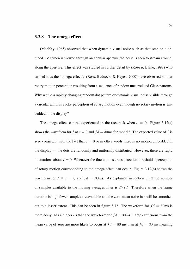
69

3.3.8 The omega effect

(MacKay, 1965) observed that when dynamic visual noise such as that seen on a de-

tuned TV screen is viewed through an annular aperture the noise is seen to stream around,

along the aperture. This effect was studied in further detail by (Rose & Blake, 1998) who

termed it as the “omega effect”. (Ross, Badcock, & Hayes, 2000) have observed similar

rotary motion perception resulting from a sequence of random uncorrelated Glass patterns.

Why would a rapidly changing random dot pattern or dynamic visual noise visible through

a circular annulus evoke perception of rotary motion even though no rotary motion is em-

bedded in the display?

The omega effect can be experienced in the racetrack when c = 0. Figure 3.12(a)

shows the waveform for I at c = 0 and fd = 30ms for model2. The expected value of I is

zero consistent with the fact that c = 0 or in other words there is no motion embedded in

the display — the dots are randomly and uniformly distributed. However, there are rapid

fluctuations about I = 0. Whenever the fluctuations cross detection threshold a perception

of rotary motion corresponding to the omega effect can occur. Figure 3.12(b) shows the

waveform for I at c = 0 and fd = 80ms. As explained in section 3.3.2 the number

of samples available to the moving averages filter is T/fd. Therefore when the frame

duration is high fewer samples are available and the zero-mean noise in e will be smoothed

out to a lesser extent. This can be seen in figure 3.12. The waveform for fd = 80ms is

more noisy (has a higher σ) than the waveform for fd = 30ms. Large excursions from the

mean value of zero are more likely to occur at fd = 80 ms than at fd = 30 ms meaning

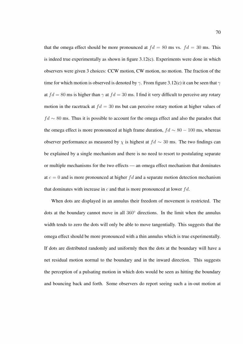
70

that the omega effect should be more pronounced at fd = 80 ms vs. fd = 30 ms. This

is indeed true experimentally as shown in figure 3.12(c). Experiments were done in which

observers were given 3 choices: CCW motion, CW motion, no motion. The fraction of the

time for which motion is observed is denoted by γ. From figure 3.12(c) it can be seen that γ

at fd = 80 ms is higher than γ at fd = 30 ms. I find it very difficult to perceive any rotary

motion in the racetrack at fd = 30 ms but can perceive rotary motion at higher values of

fd ∼ 80 ms. Thus it is possible to account for the omega effect and also the paradox that

the omega effect is more pronounced at high frame duration, fd ∼ 80 − 100 ms, whereas

observer performance as measured by χ is highest at fd ∼ 30 ms. The two findings can

be explained by a single mechanism and there is no need to resort to postulating separate

or multiple mechanisms for the two effects — an omega effect mechanism that dominates

at c = 0 and is more pronounced at higher fd and a separate motion detection mechanism

that dominates with increase in c and that is more pronounced at lower fd.

When dots are displayed in an annulus their freedom of movement is restricted. The

dots at the boundary cannot move in all 360◦ directions. In the limit when the annulus

width tends to zero the dots will only be able to move tangentially. This suggests that the

omega effect should be more pronounced with a thin annulus which is true experimentally.

If dots are distributed randomly and uniformly then the dots at the boundary will have a

net residual motion normal to the boundary and in the inward direction. This suggests

the perception of a pulsating motion in which dots would be seen as hitting the boundary

and bouncing back and forth. Some observers do report seeing such a in-out motion at

71

(a) 0 20 40 60 80 100−0.8

−0.6

−0.4

−0.2

0

0.2

0.4

0.6

0.8

Time (s)

I

(b) 0 20 40 60 80 100−0.8

−0.6

−0.4

−0.2

0

0.2

0.4

0.6

0.8

Time (s)

I

(c) 0 10 200

0.2

0.4

0.6

0.8

1

dot density

γ

c = 0 fd = 30ms

0 10 200

0.2

0.4

0.6

0.8

1

dot density

γ

c = 0 fd = 80ms

Figure 3.12: c = 0 (a) waveform of I at fd = 30 ms (b) waveform of I at fd = 80 ms (c)fraction of time γ for which rotary motion is perceived by human observers.

c = 0 as opposed to rotary motion. Figure 3.13 shows the standard deviation of I for

model2 for two cases (a) rotary motion, (b) radial motion in which the cross product in

equation 3.5 is replaced by a dot product. It is seen that as the annulus width decreases

the amount of rotary motion increases whereas the amount of radial motion decreases.

Interestingly for a fat annulus there is significant radial motion present in the stimulus;

however when I calculated σ(I) for rotary and radial motion using a model based on the

(Watson & Ahumada, 1985) motion detector I did not see the increase in σ(I) for radial

motion when the annulus width is increased (compare figure 3.13 to figure 5.5).

3.3.9 Reproducibility of observer responses

As described in the previous chapter an important characteristic of the “omega effect”

is that at c = 0 the same stimulus movie produces different responses from an observer in

different trials. This phenomenon can be explained by the fact that neurons give different

responses to the same stimulus in different trials. This uncertainty in response can be

modeled by adding a small perturbation to the dot positions or by adding some noise to the

72

0 2 4 6 8 10

0.1

0.15

0.2

0.25

inner circle (degrees)

σ(I)

rotary motionradial motion

Figure 3.13: As the width of annulus is decreased amount of rotary motion increases andamount of radial motion decreases. Model2 c = 0, fd = 30 ms, dd = 2.5 dots/degree2,outer circle=10◦.

73

signal e or I . At c = 0 the motion signal (e or I) is already so weak that the uncertainty or

noise in response overwhelms the motion signal and can even flip its polarity (+ve or -ve)

in different trials resulting in different responses to the same stimulus; as c increases the

motion signal becomes more robust and insensitive to small perturbations arising from the

uncertainty in response.

The NN model already has some stochasticity built into it. It randomly selects a dot,

matches it to its NN and repeats until enough dots are matched. Because of this randomness

it gives slightly different motion values in different trials to the same stimulus. In fact it is

found that this randomness is enough to make reproducibility zero at c = 0 as shown by

the ζ values in figure 3.14. There is no need to add additional noise to e or I . In figure

3.14 the baseline value of ζ corresponding to zero reproducibility is given by 0.11 ± 0.15

(mean±s.d.). The baseline value corresponding to zero reproducibility is not zero because

ζ is the maximal normalized cross correlation of two functions. The baseline is calculated

as the expected value of maximal cross correlation between observer responses resulting

from different stimuli being shown in different trials.

In addition to accounting for the zero reproducibility of observer responses at c = 0, the

uncertainty or cortical noise in response may also play an important part in the perception

of omega effect by stochastically boosting the weak motion signal (fig. 3.12) so that it

becomes large enough to cross detection threshold in a stochastic resonance like manner.

There is increasing evidence of the important role stochastic resonance plays in biological

systems and there is all the reason to expect that the noise level in the brain is carefully

74

0 0.02 0.04 0.06 0.08 0.10

0.2

0.4

0.6

0.8

1

dot correlation

ζexperimentNN model

Figure 3.14: Variation of ζ which is a measure of response reproducibility for a givenstimulus vs. dot correlation c.

controlled to help us detect subliminal signals that would perhaps remain undetected in

the absence of noise (Simonotto et al., 1997; Gammaitoni, Hanggi, Jung, & Marchesoni,

1998). (Fermuller, Shulman, & Aloimonos, 2001) argue that noise in response is the cause

of illusory motion perception in the Ouchi pattern.

3.4 Limitations of models

The obvious limitation of the models presented here is that they assume the dot posi-

tions are known in various frames. The models are suitable for motion detection in displays

75

consisting of identical indistinguishable features and a feature extraction step is needed to

determine the positions of features in various frames which would be input to the models.

Figure 3.15 shows model sensitivity to dot positions. The original dot positions are per-

turbed by a displacement ~d where the length of the displacement is normally distributed

with mean zero and standard deviation σ and the direction of displacement is uniformly

distributed over −π to +π. Figure 3.15(a) shows the effect of uncertainty in dot position

on χ for the NN model. Because the NN model is particularly sensitive to dot density χ

decreases more rapidly with noise at high dot density. Plotting χ against σ√

dd as in Figure

3.15(a) collapses the different curves for different dot densities onto a single curve. Figure

3.15(b) shows the effect of uncertainty in dot position on χ for model2. Since model2 is

insensitive to dot density the curves for different dot density collapse into a single curve.

The models are fairly robust to uncertainty in dot positions.

Another limitation of the models is that the differential motion signal e is computed by

taking into consideration just two successive frames. This means that if a random frame

is inserted between every pair of correlated frames of the racetrack both models will fall

apart. Why take only two successive frames into account while computing e? Why not

3? or 4? Figure 3.16 shows the values of χ when K random frames are inserted between

the correlated frames e.g. when K=1 in between every two correlated frames there is a

random frame in which all dot positions are randomly and uniformly generated. Uptil now

K was zero for all the figures. As can be seen from figure 3.16 when K is made non-

zero the χ values do not abruptly fall down to zero showing that the human visual system

76

takes multiple frames into consideration while detecting local motions. This raises two

questions: (a) How many frames should then be taken into consideration while computing

e? (b) How should information from multiple frames be combined to get an estimate of e?

This appears to be a long standing and much neglected problem in computer vision. Since

the papers of (Horn & Shunck, 1981; Lucas & Kanade, 1981) on optical flow computation,

motion estimation has been one of the most heavily researched topics in computer vision,

for reviews see e.g. (Barron, Fleet, Beauchemin, & Burkitt, 1992; Barron & Beauchemin,

1995; Galvin, McCane, Novins, Mason, & Mills, 1998; Stiller & Konrad, 1999; McCane,

Novins, Crannitch, & Galvin, 2001). Most of the optical flow algorithms including the

recent ones representing the state-of-the-art use just two frames to compute motion (Bruhn,

Weickert, & Schnorr, 2005; Brox, Bruhn, Papenberg, & Weickert, 2004; Roth & Black,

2005). Although there exist multi-frame optical flow algorithms e.g. (Irani, 1999; Shafique

& Shah, 2005; Camus, 1997) the number of frames chosen for optical flow computation is

decided in an ad hoc manner without any principled justification. I believe the answer to the

first question depends on the frame duration. The RF of local motion detectors in the human

visual system have a temporal size of 100-200 ms. Therefore all spatiotemporal signal

falling within this window should be used to compute e. This explains that when frame

duration becomes too large (� 200 ms) the motion completely disappears in the display

no matter how high c is because within a bin of 200 ms there really isn’t any motion going

on in the display. In summary, just as a spatial weighting function w (equation 3.2) has

been used that mimics the spatial component of the RF of a neuron, a temporal weighting

77

(a)0 1 2 3 4

0

0.2

0.4

0.6

0.8

1

GaussianNoiseσ * sqrt(dd)

χ

dd=1dd=5dd=10

(b)0 0.5 1 1.5 2 2.5 3

0

0.2

0.4

0.6

0.8

1

GaussianNoise σ

χ

dd=1dd=5dd=10

Figure 3.15: Effect of uncertainty in positions of dots for the two models. (a) NN, (b)Model 2. c=0.5, fd=30ms, ic=7◦.

(a)0 1 2 3 4

0

0.2

0.4

0.6

0.8

1

K

χ

c=0.1c=0.3c=0.5

(b)0 1 2 3 4

0

0.2

0.4

0.6

0.8

1

K

χ

fd=10msfd=30msfd=80ms

Figure 3.16: Effect of inserting K random frames between correlated frames for humanobservers. χ does not drop to zero level abruptly for non-zero K showing that humanobservers do not match just the consecutive 2 frames but multiple frames are taken intoconsideration. (a) χ vs. K for different dot correlation, fd=30ms. (b) χ vs. K for differentframe duration, c = 0.5.

function should also be used that would mimic the temporal response of RF of a motion

sensitive neuron. That would enable the models to deal with the case when K is non-zero.

3.5 Conclusions and Remarks

In a display consisting of identical indistinguishable features such as random dot kine-

matograms the motion correspondence problem is an artificial problem — one that does

78

not need to be solved and is probably not solved by the human visual system. The fact

that experimentally: 1) χ does not depend on dot density, 2) χ decreases and eventually

becomes zero with increase in hop size for c as high as 0.5 provides strong evidence that all

dots falling within a small patch a la receptive field of a motion sensitive cell are considered

when computing local motion. When the correlated dot lies outside the receptive field as

when happens when hop size is increased beyond a limit χ drops to zero no matter how

high c.

(Dawson, 1991) enunciates 3 principles that should guide motion correspondence: 1)

the first principle is that of nearest neighbors that says each dot will try to match to its

nearest neighbor, 2) the second principle is that of element integrity which says that the

matching should be such that splitting and fusing of dots should be avoided, 3) the third

principle is the relative velocity (RV) principle which says that the matching should be such

that all dots will tend to move in the same direction. I believe that element integrity will

hold when the number of dots is few (hardly more than 10) as was perhaps the case in the

psychophysical experiments based on which this principle is formulated. When number of

dots is few each dot stands out like an object and so element integrity applies. But as the

number of dots increases element integrity quickly disappears as it becomes very difficult

to preserve the integrity of each element. (Weiss, 1998) solves for optic flow subject to

a prior favoring a slow and smooth flow field. He is able to explain a large number of

phenomena involving sine gratings. Compare the slow and smooth examples of Weiss with

the NN and RV principles of Dawson. Further note that the form of equation 5 page 3190

79

in (Grzywacz et al., 1995) is same as the equation (Weiss, 1998) gets in his appendix 2.6 on

page 97. The main difference is that (Grzywacz et al., 1995) uses cell responses whereas

(Weiss, 1998) uses image intensity values.

The NN model takes into account the NN and element integrity principles but entirely

discounts the RV principle. It is a highly nonlinear model in which a dot matches with its

NN and the other dots have no influence on this pair. It also suffers from various other

issues such as what should be done when the number of dots changes from frame to frame.

When the features are identical and indistinguishable every dot ought to have some effect

over every dot. Model2 based on this premise is able to explain most of the psychophysical

data including dot density independence and bypasses the motion correspondence problem.

(Barlow & Tripathy, 1997) write that “the ideal detector of coherent motion would base its

decision on all the information present in the stimulus, so it would examine all possible

correspondences, and count the number of vectors for motion with the particular direction

and velocity of interest...”.

The perception of motion is critically dependent on the frame duration used. The same

sequence of frames that evoke perception of vivid motion at fd = 30 ms fail to evoke any

perception of motion whatsoever at fd � 200 ms. This is because the motion computed

by local motion detectors at time t is based on the spatiotemporal signal from time t−T to

time t where T ∼ 200 ms, so when fd � T the spatiotemporal signal is mostly constant

within a bin of duration T and local motion detectors will fail to register motion.

The experimentally observed position invariance of MST(d) cells can be explained by

80

the analysis shown in section 3.3.6. The puzzling omega effect in which a sequence of

random dot patterns in a circular annulus evokes perception of rotary motion is explained

as follows: displaying the dots in a circular annulus restricts their freedom of movement e.g.

in the limit when annulus width tends to zero the dots will only be able to move tangentially.

The random dot display gives a weak rotary motion signal with mean zero. However this

weak signal when combined with the uncertainty or noise in response can become large

enough to cross detection threshold a la stochastic resonance. The uncertainty or noise in

response also explains the zero reproducibility of observer response that is characteristic of

the omega effect — the fact that an observer gives different responses to the same stimulus

in different trials.

This chapter investigated (a) how valid is the concept of motion correspondence (b)

how much of experimental psychophysics can be explained by a model that assumes the dot

positions are known in various frames. Chapter 5 will address the limitations of the models

presented here by developing a model that is not restricted to random dot kinematograms

(RDKs) and can be applied to real world scenes also.

81

Chapter 4

An introduction to the

Watson-Ahumada (WA) motion detector

This chapter provides an introduction to the Watson-Ahumada (WA) motion detector

that is used later to model the psychophysics of the racetrack. The best place to read about

the WA detector is of course the original paper by (Watson & Ahumada, 1985).

With respect to motion estimation our objective is that given an input spatiotemporal

movie or signal denoted by L(x, y, t) we would like to output the instantaneous image ve-

locity at every position (x, y) and time t denoted by (vx(x, y, t), vy(x, y, t)). In the discus-

sion that follows, in order to illustrate the principle of operation of various motion models

we will often focus our attention on estimating the velocity (vx, vy) at a particular position

(x0, y0) and time t0 by considering the signal I(x, y, t) contained within a small causal

spatiotemporal window centered at (x0, y0, t0) as illustrated in figure 4.1. By varying the

82

Figure 4.1: A motion detection algorithm takes as input a spatiotemporal movie L(x, y, t)and outputs the instantaneous image velocity at every position (x, y) and time t denotedby (vx(x, y, t), vy(x, y, t)). The velocity (vx, vy) at a particular position (x0, y0) and timeinstant t0 is determined by the input signal contained within a small causal spatiotemporalpatch or window centered at (x0, y0, t0).

position of the patch over all (x, y) and t the velocity at all different positions (x, y) and

times t is easily found.

Let us begin by considering the motion of a sine grating. First consider a stationary sine

grating. The intensity or luminance at any position (x, y) is given by

f(x, y) = sin(ωxx + ωyy) (4.1)

where ωx and ωy are known as the spatial frequencies of the grating. If now this grating

starts moving with velocity (vx, vy) then the part of the grating at position (x, y) at time

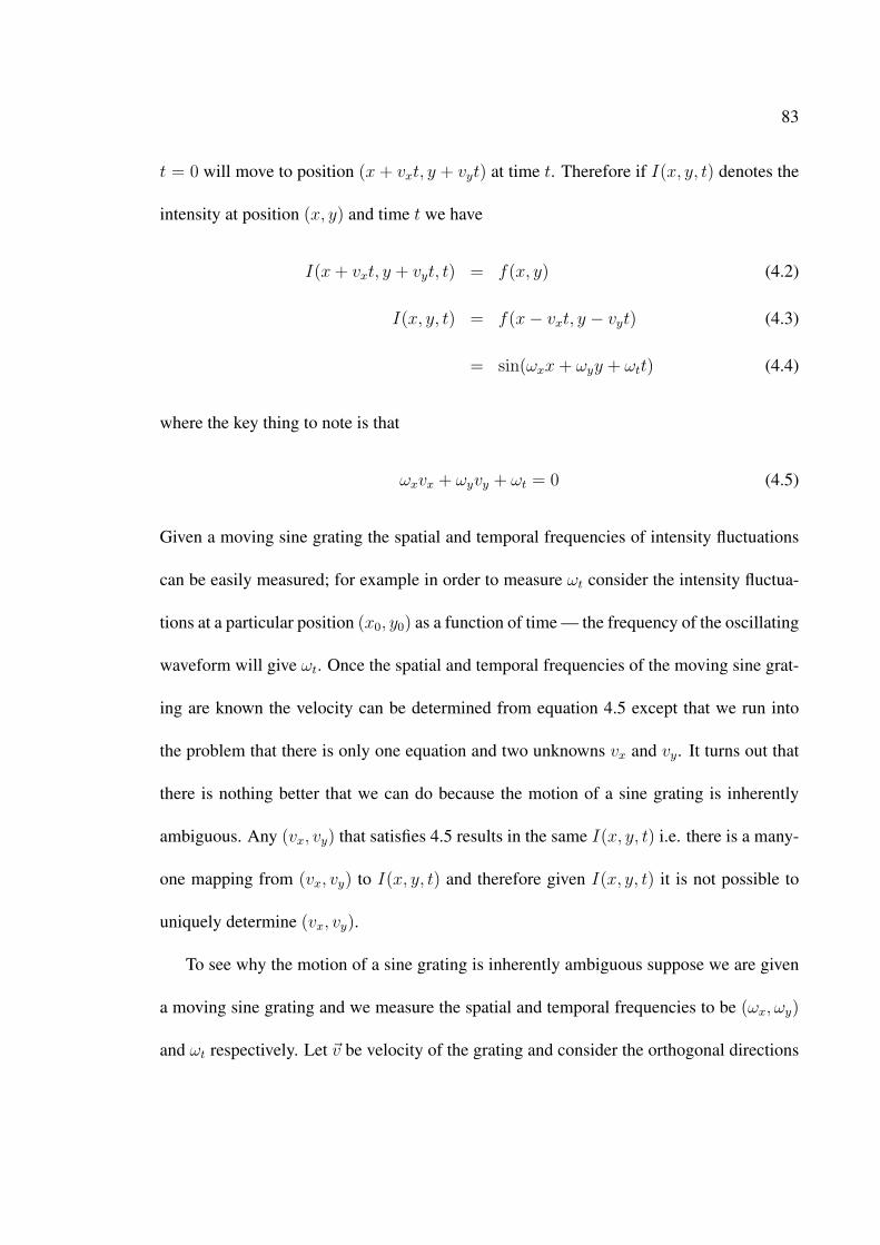
83

t = 0 will move to position (x + vxt, y + vyt) at time t. Therefore if I(x, y, t) denotes the

intensity at position (x, y) and time t we have

I(x + vxt, y + vyt, t) = f(x, y) (4.2)

I(x, y, t) = f(x− vxt, y − vyt) (4.3)

= sin(ωxx + ωyy + ωtt) (4.4)

where the key thing to note is that

ωxvx + ωyvy + ωt = 0 (4.5)

Given a moving sine grating the spatial and temporal frequencies of intensity fluctuations

can be easily measured; for example in order to measure ωt consider the intensity fluctua-

tions at a particular position (x0, y0) as a function of time — the frequency of the oscillating

waveform will give ωt. Once the spatial and temporal frequencies of the moving sine grat-

ing are known the velocity can be determined from equation 4.5 except that we run into

the problem that there is only one equation and two unknowns vx and vy. It turns out that

there is nothing better that we can do because the motion of a sine grating is inherently

ambiguous. Any (vx, vy) that satisfies 4.5 results in the same I(x, y, t) i.e. there is a many-

one mapping from (vx, vy) to I(x, y, t) and therefore given I(x, y, t) it is not possible to

uniquely determine (vx, vy).

To see why the motion of a sine grating is inherently ambiguous suppose we are given

a moving sine grating and we measure the spatial and temporal frequencies to be (ωx, ωy)

and ωt respectively. Let ~v be velocity of the grating and consider the orthogonal directions

84

given by ~e1 = ωxi + ωy j and ~e2 = ωy i − ωxj. Let us resolve ~v along ~e1 and ~e2 so that

~v = k1 ~e1 + k2 ~e2 where k1, k2 are unknown constants to be determined. Plugging ~v into the

master equation 4.5 we get

(k1ωx + k2ωy, k1ωy − k2ωx) · (ωx, ωy) + ωt = 0 (4.6)

k1(ω2x + ω2

y) + k2 · 0 + ωt = 0 (4.7)

Thus we see only k1 can be found; further any k2 ∈ R will satisfy the master equation 4.5.

Therefore the motion of the grating along ~e1 can be uniquely determined but the motion of

the grating along ~e2 is indeterminate and consistent with any choice of k2. This happens

because there is no variation in intensity of a sine grating along ~e2 and so if the grating

moves in this direction the motion cannot be discerned — the grating appears stationary

along ~e2. To see this first consider a stationary grating whose intensity pattern is given by

f(x, y) = sin(ωxx + ωyy) (4.8)

as before. Now suppose the grating moves with a velocity ~v = k(ωy i − ωxj) where k is

some known constant. Then the intensity I(x, y, t) at any position (x, y) and time t is given

by

I(x, y, t) = f(x− vxt, y − vyt) (4.9)

= f(x− kωyt, y + kωxt) (4.10)

= sin(ωx(x− kωyt) + ωy(y + kωxt)) (4.11)

= sin(ωxx + ωyy) (4.12)

= f(x, y) independent of t (4.13)

85

Thus a moving grating along ~e2 cannot be distinguished from a stationary grating. Since a

sine grating is essentially a 1D pattern when it moves its 2D velocity is ambiguous. This is

the well known aperture problem in vision and holds for the motion of any 1D pattern not

necessarily a sine grating.

What we have seen uptill now is how to estimate the motion of a sine grating. Let us

now turn our attention on how to estimate the motion of any I(x, y, t); it does not have

to be a sine grating. The Fourier Transform allows us to express any image as the sum

of an infinite number of sine gratings. If now this image moves with a velocity ~v then all

the underlying gratings will move with the same velocity ~v and their spatial and temporal

frequencies will be related by the master equation (4.5). Therefore if we can decompose

the given I into its constituent gratings and measure their spatial and temporal frequencies

we can find ~v by solving an overconstrained system of linear equations as dictated by the

master equation (4.5):

ωx1 ωy1

ωx2 ωy2

......

ωxn ωyn

·

vx

vy

= −

ωt1

ωt2

...

ωtn

(4.14)

where (ωxi, ωyi) and ωti are the spatial and temporal frequencies of the i-th grating. This is

what the WA detector does.

Another useful interpretation of the WA motion detection principle to keep in mind

is as follows: Let F(ωx, ωy) denote the fourier transform of f(x, y). Then if the image

86

undergoes translation with time such that I(x, y, t) = f(x − vxt, y − vyt) then the fourier

transform of I is given by

I(ωx, ωy, ωt) =

∫ ∫ ∫I(x, y, t)exp(−j(ωxx + ωyy + ωtt))dxdydt

=

∫ ∫ ∫f(x− vxt, y − vyt)exp(−j(ωxx + ωyy + ωtt))dxdydt

After making a change of variables u = x − vxt, v = y − vyt and some algebra above

reduces to

I(ωx, ωy, ωt) =

∫F(ωx, ωy)exp(−j(ωxvx + ωyvy + ωt)t)dt (4.15)

= F(ωx, ωy)δ(ωxvx + ωyvy + ωt) (4.16)

Therefore the fourier transform of I(x, y, t) lies on a plane whose equation is given by

ωxvx + ωyvy + ωt = 0 (4.17)

and is obtained by applying a shear to F(ωx, ωy) as illustrated in figure 4.2. This is equiv-

alent to our earlier result that the grating with spatial frequencies (ωx, ωy) will move such

that the temporal frequency is given by equation 4.5. The problem of motion estimation

can therefore also be equivalently posed as the problem of finding the best fitting plane to

the power spectrum of I(x, y, t) that passes through the origin. The equation of the plane

will give the motion as per equation 4.17.

Having looked at the basic principles behind the WA motion detection mechanism let

us now study the operation of the detector in more detail. The input stimulus L(x, y, t) is

first convolved through a number of filters in parallel as illustrated in figure 4.3. The effect

87

Figure 4.2: The fourier transform of a stationary image lies on the ωxωy plane and isdenoted by the solid plane. The effect of motion is to shear the fourier transform so that itnow lies on the plane ωxvx + ωyvy + ωt = 0. The arrows indicate the displacement of asingle spatial-frequency component (a sine grating).

88

of convolution is that at each position (x, y) the input signal within a Gaussian window is

resolved into the constituent gratings with spatial frequencies ~ki = (k cos θi, k sin θi) where

θ = {0, 36◦, 72◦, . . . , 324◦}; θi = 36◦i with i ∈ [0, 9]. k determines the scale of interest.

The power spectra of the filters are illustrated in figure 4.4 and have the appearance of

candlelight shaped blobs with bases centered at ~ki. We have seen that the power spectrum

of a translating image lies on the plane ωxvx + ωyvy + ωt = 0. Half of this plane will be

above the ωxωy plane and half will be below the ωxωy plane. This means given a perfect

input only half of the filters will give non-zero response because only half of the filters

will intersect the ωxvx + ωyvy + ωt = 0 plane. Further the temporal frequencies of filter

responses will be governed by the master equation

ωxvx + ωyvy + ωt = 0 (4.18)

letting (ωx, ωy) = k(cos θ, sin θ) where θ changes with the filter and (vx, vy) = v(cos α, sin α)

above simplifies to

ωt = −kv cos(θ − α) (4.19)

Therefore ωt vs. θ will be a sinusoid waveform; only half of the sinusoid will be present

as half of the sensors will be silent. The position of the maxima occurs at θ = α which

is the direction of motion and the height of the maxima is proportional to v. Therefore by

measuring the temporal frequencies of filter responses and pooling the responses to locate

the position and height of the maxima of ωt vs. θ the local motion at each position (x, y)

can be estimated. A picture of the local motion vectors at each position (x, y) is known as

the optical flow map.

89

Figure 4.3: The WA motion detection pipeline. The input is first convolved through a num-ber of filters in parallel. The temporal frequencies of filter responses contain informationabout the velocity as per equation 4.19. The filter responses have to be pooled to estimatethe motion.

90

Figure 4.4: Power spectra of the filters in figure 4.3. Each different color corresponds to adifferent filter. Only the +ve half of ωt space is shown. Since the filters model V1 simplecells and therefore must have real valued impulse responses the power spectra in −ve halfof ωt can be obtained using the identity P (ωx, ωy, ωt) = P (−ωx,−ωy,−ωt).

91

(DeAngelis et al., 1995) and others have found that the WA filters provide an accurate

model of simple cell receptive fields (RFs). Quoting from (DeAngelis et al., 1996):

Rather, simple cell RFs in the joint space-time domain appear to be fit well by amodel first proposed by Watson and Ahumada (4, 5). To the best of our knowl-edge, their papers and that by Adelson and Bergen (6) are the first to presentthe notion of oriented receptive fields in the joint space-time domain, as wellas the idea of space-time separability or inseparability. We have acknowledgedthese papers in our review in TINS (7). The Watson and Ahumada model isbased on a pair of simple cells that are space-time separable and in quadra-ture, which means that the space and time RFs of each cell of the pair, areHilbert transforms of the other’s (with approximations to satisfy the causalityconstraint for the time domain). Based on the Watson-Ahumada formulation,we have modelled space-time RFs of simple cells, as the weighted sum of twospace-time separable subunits in a quadrature relationship. This model formu-lation provides a remarkably good fit to the data from most cells, regardless oftheir degree of space-time inseparability (8).

In conclusion, to account for space-time RFs of simple cells that differ widelyin the degree of space-time inseparability, at least two separable subunits ap-pear necessary as modelled by Watson and Ahumada (5).

The impulse response of a WA filter has the following analytic form:

h(x, y, t) = exp

(−x2 + y2

λ2

) [cos(~k · ~x)f(t) + sin(~k · ~x)fq(t)

](4.20)

where ~k = k(cos θ, sin θ) and ~x = (x, y). f(t) is derived from the temporal contrast-

sensitivity data of human observers to relatively low spatial frequencies. Its analytical

form can be found in (Watson & Ahumada, 1985). fq(t) is the Hilbert transform of f(t)

together with an appropriate time delay to ensure that h corresponds to a causal filter.

λ =6√

ln 2

k(4.21)

This choice of λ results in a filter with a bandwidth of 1 octave. The response of the sensor

located at (x, y) at time t is given by L(x, y, t) ∗ h(x, y, t) where L is the input.

92

This is the right place to make a distinction between the WA sensors and Adelson-

Bergen (AB) motion energy detector (Adelson & Bergen, 1985). The WA sensor adds the

responses of the main and quadrature path whereas in (Adelson & Bergen, 1985) the main

and quadrature responses are squared and then added together. The response of the motion

energy detector located at (x, y) is given by

r(t) = r2m(t) + r2

q(t) (4.22)

where rm and rq are the responses of the main and quadrature paths given by L ∗ hm and

L ∗ hq respectively with

hm = exp

(−x2 + y2

λ2

)cos(~k · ~x)f(t) (4.23)

hq = exp

(−x2 + y2

λ2

)sin(~k · ~x)fq(t) (4.24)

If the main and quadrature filters are approximated by odd and even Gabors tuned to

(ωx0, ωy0, ωt0) then the function of AB motion energy detector is to take a local Fourier

Transform of the input spatiotemporal signal at every position (x, y, t) and evaluate the

value of the power spectrum at the frequency (ωx0, ωy0, ωt0). This is proved in section 4.5.

For the topic of how to use motion energy detectors to compute motion see (Heeger, 1987).

The (Watson & Ahumada, 1985) model allows for computation of motion at different

spatial scales by adjusting the center frequency k of the filters in equation 4.20. The filters

tuned to higher spatial frequencies have smaller RF and are tuned for detecting smaller

displacements. This is nicely illustrated by running the model on a display of random dots

undergoing radial motion. Such a display was created with radial hop size h = 0.0871r

93

degrees where r is distance of dot from the center measured in degrees; c = 0.6 mem-

oryless, fd = 25 ms. The screen measured 12.46×12.46 degrees or 512×512 pixels.

Dots were displayed in the central 10◦ circle of the screen. The optical flow computed at

scales corresponding to center frequencies of {1/4, 1/8, 1/16, 1/32, 1/64} cycles/pixel or

{10.275, 5.13, 2.56, 1.28, 0.64} cycles/degree are shown in figures 4.5 to 4.9 respectively.

As these figures illustrate the scales tuned to higher spatial frequencies with smaller RFs

cannot capture the large displacements that occur further out from the center. The scales

tuned to lower spatial frequencies have large RFs and are ideally suited for capturing the

overall motion field. All results for the model in Chapter 5 are computed at a scale of 0.64

cycles/degree unless stated otherwise.

4.1 At what rate should motion be sampled to make ap-

parent motion indistinguishable from continuous mo-

tion?

When a sequence of discrete snapshots of a moving object are presented to the eye in

rapid succession it creates the illusion of smooth real motion. This principle of apparent

motion is the basis of movies, cinema and even the experiments described in this disser-

tation. Before discussing the requirements on the sampling rate in order to produce the

illusion of smooth motion let us clarify the distinction between staircase motion and stro-

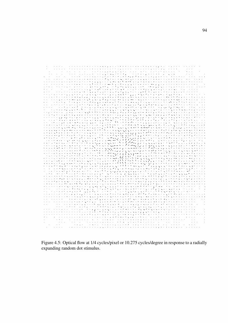
94

Figure 4.5: Optical flow at 1/4 cycles/pixel or 10.275 cycles/degree in response to a radiallyexpanding random dot stimulus.

95

Figure 4.6: Optical flow at 1/8 cycles/pixel or 5.13 cycles/degree in response to a radiallyexpanding random dot stimulus.

96

Figure 4.7: Optical flow at 1/16 cycles/pixel or 2.56 cycles/degree in response to a radiallyexpanding random dot stimulus.

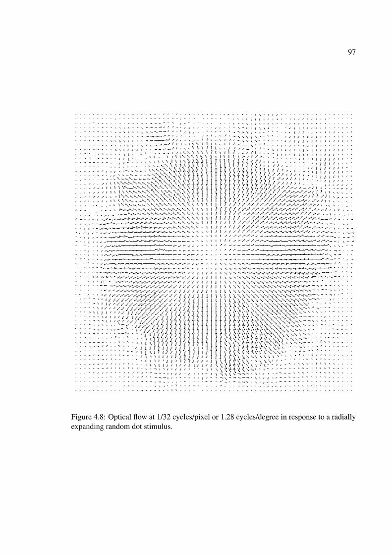
97

Figure 4.8: Optical flow at 1/32 cycles/pixel or 1.28 cycles/degree in response to a radiallyexpanding random dot stimulus.

98

Figure 4.9: Optical flow at 1/64 cycles/pixel or 0.64 cycles/degree in response to a radiallyexpanding random dot stimulus.

99

(a) (b)

(c)

Figure 4.10: x− t spacetime plots for a particle moving with constant velocity (a) contin-uous motion (b) stroboscopic motion (c) staircase motion

boscopic motion. The distinction is provided by figures 4.10(a),(b),(c) which show the

x − t spacetime plots of a particle moving with constant velocity for continuous, strobo-

scopic and staircase motion respectively. All experiments in this dissertation are examples

of staircase motion. The sampling requirements for stroboscopic and staircase cases are

largely the same.

Consider a particle moving with speed v. The position of the particle is given by

x(t) = vt (4.25)

The Fourier transform of x(t) is given by

X(ω) =

∫ T

0

x(t) exp(−jωt)dt (4.26)

the Fourier transform is taken in a window of duration T where T is the temporal size of

the RF of local motion detectors in V1/MT, the idea being that the local motion detector is

100

sensitive only to what happens in a time interval of duration T . It is found that

X(ω) =vT 2

θ2(jθ exp(−jθ) + exp(−jθ)− 1) (4.27)

|X(ω)|2 =v2T 4

θ4

(θ2 + 2− 2 cos(θ)− 2θ sin(θ)

)(4.28)

where θ = ωT . The FWHM (full width at half maximum) of |X(ω)|2 denoted by ω0 is

found as

ω0 =6.95

T(4.29)

f0 =ω0

2π=

1.1

T(4.30)

Note that f0 does not depend on v the velocity of the particle. To avoid any aliasing,

sampling must be done at a rate f sufficiently higher than f0 or equivalently the frame

duration should be sufficiently less than T . This result makes intuitive sense because if fd

is not sufficiently less than T e.g. when fd is of the order of T then the input sampled

signal is mostly constant within a window of duration T or put it another way not enough

samples are available and therefore no motion can be computed or the motion estimate will

be wrong. At a frame rate of 30Hz which is well known to produce seamless motion

f

f0

∼ 5.5 (4.31)

using T = 200 ms. If the Nyquist rate is taken to be 2f0 then 30Hz corresponds to sampling

at 2.75 times the Nyquist rate.

The question of what rate to sample was also considered by (Watson & Ahumada,

1983; Watson, Ahumada, & Farrell, 1986); also see (Morgan, 1980). Whereas the above

101

analysis took as input the function relating displacement to time (equation 4.25) (Watson &

Ahumada, 1983; Watson et al., 1986)’s analysis takes as input the function relating contrast

to space and time and their theory is that if this function does not change within the limits

of the spatiotemporal window of visibility after sampling then the observer will not be able

to distinguish the sampled motion from continuous motion. (Watson & Ahumada, 1983;

Watson et al., 1986) get a plausible formula for the critical sampling rate as

ωc = ωl + vul (4.32)

where ωc is the critical sampling rate for no aliasing, ωl and ul are limits of temporal and

spatial frequency detectable by humans (the boundaries of the spatiotemporal window of

visibility1). Note the dependence of ωc on v the velocity of particle. They report results

of a psychophysical experiment (fig. 5 in (Watson & Ahumada, 1983)) to test the formula.

Two displays are shown to an observer — one is continuous motion the other is sampled

motion. The observer tries to pick the display having sampled motion. However, with

respect to figure 5 in (Watson & Ahumada, 1983) at the critical sampling rate the observer

should be taking guesses and so should be wrong about 50% of the time. But the figure

caption says that at the critical sampling rate observer is right 75% of the time! Also the

values of the critical sampling rate reported seem to be too high e.g. at v = 0 the critical rate

is found as 30-40Hz but it is well known that 30Hz works beautifully in movies suggesting

it should be well above the critical sampling rate.

1(Watson & Ahumada, 1983) use a rectangular window of visibility whereas (Adelson & Bergen, 1985)p. 292 use a diamond shaped window

102

4.2 Why can’t we see things that move too slowly or too

fast?

Based on our daily experience it is difficult to discern the motion of objects that move

very slowly (e.g. the sun, hour hand on a clock) or very fast (e.g. a fan) and so we expect

the velocity of a moving object plays a role as to how well its motion can be perceived. For

optimal response of motion sensitive cells the velocity of the target should be such that the

target spans across the RF of the cell within a time interval T . If L denotes the spatial size

of the RF then L = vT for optimal response.

Consider three cases: (i) v � L/T . In this case the target stays largely at the same

location within the RF. Recall that in the WA model the velocity is encoded in the frequency

of cell response. When v � L/T the response will be a very slowly varying function of

time as illustrated in figure 4.11(a) and the frequency cannot be accurately estimated. (ii)

v ∼ L/T in this case the response is optimal and looks like a nice sinusoid as illustrated in

figure 4.11(b) (iii) v � L/T in this case the target will quickly jump out of the RF of the

neuron and the response may look like something in figure 4.11(c). In addition to the poor

response the intrinsic clock-rate at which the motion detection circuitry operates may not

be high enough to accurately measure the frequency of the sinusoid. Note very carefully

the distinction between the rate at which continuous-time motion signal is sampled and the

intrinsic clock-rate at which the motion detection circuitry works. In this section we have

conveniently neglected any effects of sampled motion and assumed the input is continuous-

103

Figure 4.11: Response of a motion-sensitive cell as a particle moves across its receptivefield. Velocity of particle = v. Spatial size of receptive field = L. Temporal size of receptivefield = T . (a) v � L/T (b) v ∼ L/T (c) v � L/T .

104

time motion.

Finally for completeness the following paragraph discusses the gradient based approach

to motion estimation which is the de-facto method of choice for optical flow estimation in

computer vision.

4.3 Gradient based approaches

If an image undergoes translational motion with constant velocity then the total time

derivative of the intensity will be zero (conservation of intensity)

dI

dt= 0 (4.33)

or Ixvx + Iyvy + It = 0 (4.34)

where Ix, Iy, It denote partial derivatives of I with respect to x, y, t respectively. Above

result can also be derived using a Taylor series expansion

I(x, y, t + dt) = I(x− vxdt, y − vydt, t) (4.35)

= I(x, y, t)− Ixvxdt− Iyvydt + higher order terms (4.36)

dividing both sides by dt and taking the limit dt→ 0 higher order terms vanish and we get

the previous gradient constraint equation.

Ixvx + Iyvy + It = 0 (4.37)

Equation (4.37) is the more general version of equation (4.5). This equation can be used to

find the velocity except that we run into the aperture problem: one equation, two unknowns.

105

To overcome the problem take a window centered at (x0, y0) where ~v is to be estimated and

assume ~v does not change in the window. This results in an overconstrained system of

equations:

Ix1 Iy1

Ix2 Iy2

......

Ixn Iyn

·

vx

vy

= −

It1

It2

...

Itn

(4.38)

where Ixi, Iyi, Iti are partial derivatives of I with respect to x, y, t at the i-ith pixel in the

window. For further details refer to (Lucas & Kanade, 1981; Baker & Matthews, 2004).

All of the above approaches to motion detection are equivalent in the sense that they all

solve the following problem: Assume the brightness constancy/gradient constraint

I(x, y, t) = I(x− vxt, y − vyt, 0) (4.39)

which can also be written as

Ixvx + Iyvy + It = 0 (4.40)

holds for some ~v and find this ~v. The equivalence of various approaches is discussed

in (E. P. Simoncelli, 1993). Several excellent papers providing a review, discussion and

comparison of various techniques used for motion estimation already exist in the literature

see e.g. (Barron et al., 1992; Barron & Beauchemin, 1995; Galvin et al., 1998; McCane et

al., 2001).

106

4.4 Conclusion

This chapter provided an introduction to the Watson-Ahumada (WA) motion detector

that is used later in this dissertation to model the psychophysics of the racetrack. We began

by discussing the motion of a sine grating and saw that the spatial and temporal frequen-

cies of a moving sine grating have to be related by equation (4.5). Therefore by measuring

the spatial and temporal frequencies of a sine grating its velocity can be estimated. To

find the motion of a general image we can resolve the image into constituent gratings of

certain known candidate spatial frequencies, measure the temporal frequencies of intensity

variations and derive the motion of the image. We also saw that the fourier transform of a

stationary image lies on the ωxωy plane and the effect of motion is to shear the plane into a

new plane whose equation is given by equation (4.5). Thus the problem of motion detection

can also be posed as the problem of finding the best fitting plane to the power spectrum of

the spatiotemporal input. The relationship of the WA detector to the neurobiology of mo-

tion sensitive cells in the brain was briefly touched upon and it has been found that the WA

filters provide an accurate model of simple cell RFs in the brain. We also compared the WA

detector with AB motion energy detector and noted that the WA sensor adds the responses

of the main and quadrature path whereas in AB the main and quadrature responses are

squared and then added together. Finally the chapter also discussed some other techniques

used for motion detection and pointed to the equivalence of different approaches.

107

4.5 Appendix 1: Effect of convolution with a Gabor

The Fourier Transform of a signal I evaluated at a particular frequency (ωx0, ωy0, ωt0)

is given by

I(ωx0, ωy0, ωt0) =

∫ ∫ ∫I(u, v, w) exp(−j(ωx0u + ωy0v + ωt0w))dudvdw (4.41)

Suppose we want to take the Fourier Transform of I within a small Gaussian window

centered at (x, y, t). Then it will be given by∫ ∫ ∫I(u, v, w) exp(−(u− x)2 + (v − y)2 + (w − t)2

2σ2)

exp(−j(ωx0(u− x) + ωy0(v − y) + ωt0(w − t)))dudvdw

(4.42)

What happens if we convolve I with

h(u, v, w) = exp(−u2 + v2 + w2

2σ2) exp(+j(ωx0u + ωy0v + ωt0w)) (4.43)

which is the complex Gabor kernel tuned to (ωx0, ωy0, ωt0). We get

I ∗ h =

∫ ∫ ∫I(u, v, w)h(x− u, y − v, t− w)dudvdw (4.44)

=

∫ ∫ ∫I(u, v, w) exp(−(x− u)2 + (y − v)2 + (t− w)2

2σ2)

exp(+j(ωx0(x− u) + ωy0(y − v) + ωt0(t− w)))dudvdw

(4.45)

This is same as equation 4.42. Therefore the effect of convolving I with a Gabor tuned to

(ωx0, ωy0, ωt0) is to take a local Fourier Transform at every point (x, y, t) and evaluate the

Fourier Transform at the frequency (ωx0, ωy0, ωt0). If the main and quadrature filters of AB

model are approximated by odd and even Gabors tuned to (ωx0, ωy0, ωt0) then the output of

Adelson-Bergen motion energy detector is simply |I ∗ h|2.

108

Chapter 5

Modeling visual motion perception with

the Watson-Ahumada (WA) motion

detector

5.1 Introduction

In this chapter I develop a model based on the Watson-Ahumada (WA) motion detector

to explain the experimental psychophysical results. It will be shown that the model is able

to explain most of the important psychophysical data such as the delicate effects of frame

duration on motion perception, observer independence to dot density in the display and

the surprising reverse phi motion caused by contrast reversing dots. In addition the model

does not suffer from the limitations of the models in chapter 3 e.g. it can be applied to any

109

general stimulus not necessarily random dot kinematograms (RDKs). So without further

ado let us begin with the model description.

5.2 Model Description

Figure 5.1(a) shows a block schematic of the model to model observer responses to the

racetrack. The stimulus is first input to the Watson-Ahumada (WA) (Watson & Ahumada,

1985) motion detector which at time t gives the instantaneous optical flow field of the

stimulus as would be perceived by a human observer. Figure 5.1(b) shows an instance of

the optical flow field at some arbitrary time in response to a stimulus with a high value of

c. As can be seen from figure the arrows are oriented representing strong CCW motion.

The optical flow can be easily converted into an estimate of rotary motion by taking cross

products of the vectors in figure with the radial vector followed by summation or averaging.

Define

e =

∑i(ri × vi)wi∑

i wi

(5.1)

where ri, vi and wi denote radial vector, velocity vector and a weight reflecting the confi-

dence of the model in the estimated value of velocity. A graph of e is shown in figure 5.1(c).

Neurons exhibit an intrinsic variability in their response. Even a single neuron gives dif-

ferent responses to the same stimulus in different trials. This intrinsic variability in neural

response which I also refer to as intrinsic cortical noise will manifest itself as uncertainty

in motion estimation. The uncertainty or noise in response is modeled by adding Gaussian

110

(a)

(b)

(c)

0 10 20 30 40 50 60−1

0

1

e

0 10 20 30 40 50 60−5

0

5

e+G

WN

0 10 20 30 40 50 60−1

0

1

I

0 10 20 30 40 50 60−1

01

Time (s)

mot

ion

inputmodel response

Figure 5.1: (a) Block schematic of the model (b) Optical flow (c) Model response at variousother stages in the pipeline

111

White Noise (GWN) n(t) to e(t). It will be argued later on that the noise plays an important

part in the perception of motion at low values of c by stochastically boosting the weak mo-

tion signal so that it becomes large enough to occasionally cross the perceptual threshold

for rotary motion. The noise is also the reason why observers give different responses to

the same stimulus in multiple trials at c = 0. The rest of the steps in the model are same as

those for models in chapter 3. The signal e is calculated based on the instantaneous optical

flow. The human visual system must integrate information over a certain interval of time

to compute a reliable estimate of motion. This is achieved by means of a moving averages

filter whose purpose is to combine information over time, to smooth out e and remove the

high frequency noisy fluctuations in e. The output of the moving averages filter is denoted

by I . The size of the moving averages filter is the time interval over which the human

visual system is believed to integrate motion information. I choose a size of 0.5s consis-

tent with values of temporal integration window reported e.g. in (Grzywacz et al., 1995).

While doing psychophysical experiments the only information available is the direction in

which the observer is seeing motion. Therefore in order to compare model response with

experimental psychophysics the signal I needs to be converted into judgements of CCW or

CW motion which can then be compared with the judgements given by human observers.

To achieve this, the signal I is passed through a level crossing detector (LCD) with thresh-

olds ±B. Whenever I crosses +B in the +ve direction the LCD declares motion in CCW

direction and whenever I crosses −B in the -ve direction the LCD declares motion in CW

direction. B is chosen to be twice the standard deviation in I at c = 0; this makes the events

112

when I may cross detection threshold even though there is no rotary motion in the stimulus

fairly unlikely. The output of the LCD detector is shown in figure 5.1 together with the

input function that indicates the actual motion embedded in the stimulus. As before the

two curves in figure 5.1(c) can be cross correlated and the maximum value of the cross

correlation function denoted by χ indicates the model performance which can be compared

with the value of χ given by human observers.

The only free parameter in the model now is the amount and quality of noise n(t). As

described before experimentally it has been found that at c = 0 observers give completely

different responses to the same stimulus in multiple trials. The observer response repro-

ducibility is zero and the reproducibility steadily increases with increase in c. Accordingly

I increased the amount of noise in the model until it was sufficient to result in zero re-

producibility of model response at c = 0. This is shown in figure 5.2 which plots ζ vs.

k = σ(GWN)/σ0 at c = 0; σ0 stands for σ(e) at c = 0. The dotted line represents the

threshold below which ζ values can be taken to imply zero reproducibility. It is found that

model reproducibility becomes zero when k ∼ 6. Accordingly the amount of noise was

fixed at this value in the model.

In the following section I compare model results with those of experiment. In some

figures for comparison purposes two curves are shown for the model: one in which no

noise is added i.e. k = 0 and another in which noise is added with k = 6. For the figures

in which only one curve is shown for the model the curve is understood to be with noise

(k = 6).

113

0 2 4 6 80

0.2

0.4

0.6

0.8

1

σ(GWN)/σ0

ζ

Figure 5.2: Variation of model reproducibility with noise at c = 0. The dotted line repre-sents the threshold below which ζ values can be taken to imply zero reproducibility.

114

5.3 Results

5.3.1 Stochastic Resonance effects

Stochastic Resonance (SR) is a phenomenon in which the addition of noise to a non-

linear system actually improves its performance. Since its discovery by (Benzi, Sutera, &

Vulpani, 1981) SR has attracted significant attention and there is now a considerable body

of literature on the role SR may play in biological systems including humans (Moss, Ward,

& Sannita, 2004; Riani & Simonotto, 1994; Simonotto et al., 1997; Mori & Kai, 2002;

Kitajo, Nozaki, M.Ward, & Yamamoto, 2003; Gammaitoni et al., 1998). At first, the phe-

nomenon seems surprising because noise is usually thought of as being bad for a system.

Figure 5.3(a) shows a graph of χ which measures signal detectability vs. noise at c = 0.05.

It is found that the graph exhibits a peak: the characteristic signature of SR. It is to be

noted that in figure 5.3(a) the LCD threshold is fixed equal to 2σ(I) at c = 0 with k = 6

and not allowed to vary as the amount of noise changes. This is the normal usage when

showing SR in a non-dynamical or threshold based system e.g. see (Gingl, Kiss, & Moss,

1995). In figure 5.2 on the other hand the threshold was allowed to vary as the level of noise

changed; the threshold was set to 2σ(I) and varied as σ(I) varied with change in n(t). If

the LCD threshold is allowed to vary with noise as in figure 5.2 the resulting χ vs. noise

graph is shown in figure 5.3(b). This graph does not show any SR and taken together fig-

ures 5.3(a,b) reflect the important fact that just as for a given threshold there is an optimum

noise level for optimum performance conversely for a given amount of noise the threshold

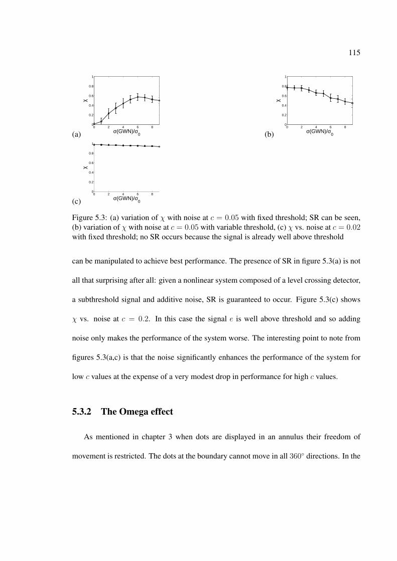
115

(a)0 2 4 6 8

0

0.2

0.4

0.6

0.8

1

σ(GWN)/σ0

χ

(b)0 2 4 6 8

0

0.2

0.4

0.6

0.8

1

σ(GWN)/σ0

χ

(c)0 2 4 6 8

0

0.2

0.4

0.6

0.8

1

σ(GWN)/σ0

χ

Figure 5.3: (a) variation of χ with noise at c = 0.05 with fixed threshold; SR can be seen,(b) variation of χ with noise at c = 0.05 with variable threshold, (c) χ vs. noise at c = 0.02with fixed threshold; no SR occurs because the signal is already well above threshold

can be manipulated to achieve best performance. The presence of SR in figure 5.3(a) is not

all that surprising after all: given a nonlinear system composed of a level crossing detector,

a subthreshold signal and additive noise, SR is guaranteed to occur. Figure 5.3(c) shows

χ vs. noise at c = 0.2. In this case the signal e is well above threshold and so adding

noise only makes the performance of the system worse. The interesting point to note from

figures 5.3(a,c) is that the noise significantly enhances the performance of the system for

low c values at the expense of a very modest drop in performance for high c values.

5.3.2 The Omega effect

As mentioned in chapter 3 when dots are displayed in an annulus their freedom of

movement is restricted. The dots at the boundary cannot move in all 360◦ directions. In the

116

limit when the annulus width tends to zero the dots will only be able to move tangentially.

If dots are distributed randomly and uniformly then the dots at the boundary will have a

net residual motion normal to the boundary and in the inward direction. This suggests the

perception of a pulsating motion in which dots would be seen as hitting the boundary and

bouncing back and forth. Some observers do report seeing such a in-out motion at c = 0

as opposed to rotary motion. Figure 5.5 shows the standard deviation of I for two cases (a)

rotary motion, (b) radial motion in which the cross product in equation 5.1 is replaced by

a dot product. Compare figure 5.5 with figure 3.13. From figure 5.5 it is seen that as the

annulus width decreases the amount of rotary motion increases whereas there is not much

change in the amount of radial motion. In figure 5.5 the values of σ(I) are the values that

result when amount of noise is zero. I chose not to add any noise in figure 5.5 to bring out

more clearly the changes that occur in the optical flow as annulus width is varied. In figure

5.5 the angle subtended by the outer circle is fixed at 10◦ visual angle and as usual ic denotes

the angle subtended by the inner circle diameter at the eye. The figure shows that as per

the model there are equal amounts of radial and rotary motion in the stimulus for ic < 6◦

whereas the rotary motion becomes increasingly dominant for ic > 8◦. This means that

the omega effect should become more pronounced for a thin annulus and should vanish for

a thick annulus. These predictions of the model are in close agreement with experimental

observations.

Figure 5.6 shows the variation of response reproducibility ζ vs. c. At c = 0 the response

reproducibility is zero and it steadily increases with increase in c as the motion signal

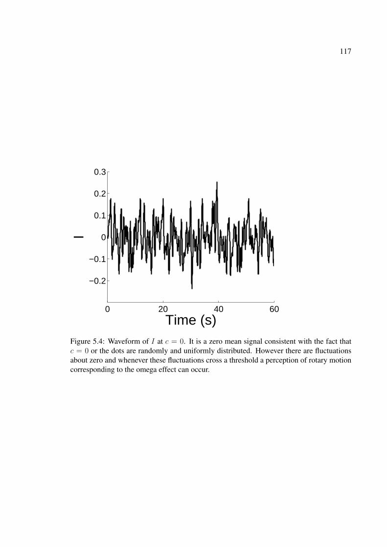
117

0 20 40 60

−0.2

−0.1

0

0.1

0.2

0.3

Time (s)

I

Figure 5.4: Waveform of I at c = 0. It is a zero mean signal consistent with the fact thatc = 0 or the dots are randomly and uniformly distributed. However there are fluctuationsabout zero and whenever these fluctuations cross a threshold a perception of rotary motioncorresponding to the omega effect can occur.

118

0 2 4 6 8 100

0.02

0.04

0.06

0.08

inner circle (degrees)

σ(I)

rotary motionradial motion

Figure 5.5: σ(I) at c = 0. For ic < 6◦ the rotary and radial motions cancel out and theomega effect disappears whereas for ic > 8◦ the rotary motion and hence the omega effectbecomes increasingly dominant.

119

0 0.02 0.04 0.06 0.08 0.10

0.2

0.4

0.6

0.8

1

dot correlation

ζmodelhumans

Figure 5.6: Response reproducibility ζ vs. c. Both model and humans show zero repro-ducibility at c = 0 and the reproducibility steadily increases with c as the motion signalgets stronger and more impervious to noise.

becomes stronger and less degraded by the noise.

5.3.3 Effect of dot correlation c

Figure 5.7(a) shows variation of signal detectability χ vs. the c. A χ value of 1 means

perfect detection and χ at c = 0 reflects the baseline zero level of χ representing chance

detectability. At c = 0 the input function does not have physical significance since there

are no dots correlated according to the input function. The χ value at c = 0 is not zero

however since χ is the maximum value of the cross correlation function between input and

response within a window of [0,4] seconds. The increase in χ with c is easy to understand

120

(a)0 0.1 0.2 0.3 0.4 0.5

0

0.2

0.4

0.6

0.8

1

dot correlation

χ

modelhumans

(b)0 0.1 0.2 0.3 0.4 0.5

0

0.5

1

1.5

2

2.5

dot correlation

τ (s

)

modelhumans

Figure 5.7: (a) χ vs. c (b) τ vs. c. fd=30 ms, ic = 7◦, dd = 5 dots/deg2

as the value of c directly expresses the amount of motion embedded in the stimulus. As

can be seen from the figure the model fits the experimental data very closely. Figure 5.7(b)

shows a graph of the reaction time τ vs. c.For c ∼ 0 τ is about 1.5s and steadily decreases

with increase in c — it takes less time to recognize the motion signal as the signal gets

stronger. At high values of c τ is about 0.5s. The model is seen to fit the experimental data

well.

5.3.4 Reverse Phi motion

If the racetrack stimulus is modified such that the correlated dots flip their polarity as

they rotate meaning black dots change to white and vice-versa then a striking phenomenon

known as the reverse-phi motion originally discovered by (Anstis & Rogers, 1975) takes

place. It is found that the motion perceived by an observer is opposite to the physical

displacement of the correlated dots or the motion embedded in the stimulus i.e. if the

correlated dots move CCW(CW) observer perceives motion in CW(CCW) direction. I find

121

that the model is able to capture this remarkable phenomenon as shown in figure 5.8. In

figure 5.8 χ is defined as the minimum value of the cross correlation function between the

response and input function within a window of [0,4] seconds.

The physical basis for the reverse phi motion can be understood as follows: It is well

known (Watson & Ahumada, 1985) that if an image is undergoing perfect translational

motion with velocity ~v = (vx, vy) i.e. if

I(x + vxt, y + vyt, t) = I(x, y, 0) (5.2)

where I(x, y, t) is the luminance/contrast at position (x, y) and at time t then the Fourier

transform of I(x, y, t) denoted by I(ωx, ωy, ωt) lies on a plane that passes through the

origin and whose equation is given by

vxωx + vyωy + ωt = 0 (5.3)

The problem of motion detection is now reduced to the problem of finding a plane that (i)

passes through the origin, (ii) captures as much energy as possible of the power spectrum

of I . The equation of the plane then tells the velocity as per equation 5.3.

Now consider a 1D particle undergoing translational motion while flipping its polar-

ity/contrast as illustrated in figure 5.9(a). The contrast of the particle is a periodic square

wave. Let f(t) be a periodic square wave with period T . Then

I(x, t) = f(t)δ(x− vt) (5.4)

where v is the velocity of the particle. The WA motion detector would take the Fourier

transform of I(x, t) and find the best fitting line of the form uωx + ωt = 0. u would then

122

give the velocity of the particle as estimated by the motion detector. We find

I(ωx, ωt) =

∫ ∫I(x, t) exp(−j(ωxx + ωtt))dxdt

=

∫ ∫f(t)δ(x− vt) exp(−j(ωxx + ωtt))dxdt

=

∫f(t) exp(−j(ωxv + ωt)t)dt

The Fourier transform of f(t)

F (ω) =

∫f(t) exp(−jωt)dt (5.5)

is given by the Fourier Series of a periodic square wave which is zero everywhere except at

ω = nω0 with ω0 =2π

T(5.6)

Further if the square wave alternates between +A and −A then the dc component of f(t):

F (0) = 0 (5.7)

Therefore we see that I(ωx, ωt) is zero everywhere except at ωxv + ωt = nω0 where n is

a non-zero integer. This is illustrated in figure 5.9(b). Note in particular that I(ωx, ωt) is

zero on the line ωxv + ωt = 0. To find the best fitting line of the form ωxu + ωt = 0 it is

immediately noted that u = v is the least likely candidate. All lines with u 6= v actually

capture equal amount of energy of I(ωx, ωt) and so fit I(ωx, ωt) equally well and there is

no unique answer for u. Since ωxv + ωt = 0 is the line that fits worst we may choose

the perpendicular line ωx(−1v

) + ωt = 0 as the best fitting line. If we take into account

the fact that the human visual system is sensitive only to a limited range of spatiotemporal

123

frequencies the so called window of visibility shown as a dotted square in figure 5.9(b)

then this provides further reason for choosing ωx(−1v

) + ωt = 0 as the best fitting line. The

velocity estimated by the motion detector is then

u = −1

v(5.8)

The -ve sign means that the motion perceived should be in opposite direction of the actual

physical displacement of the particle which is the reverse phi effect. The appearance of v in

the denominator means a faster moving particle should actually appear as moving slower!

This surprising prediction of the model is actually true within appropriate range: a display

of alternating black and white stripes was made. The width of a stripe was 0.25◦. The stripe

pattern was translated to the right and the stripes reversed their contrast after a time interval

T . On viewing the display motion is seen in the leftward direction instead of right. With

fd = T = 30 ms and a hop size of 0.125◦ the pattern appears to be moving slower than

with hop size of 0.0625◦.

As another example suppose a display of random black and white bars is moved to the

right at a constant velocity. The spacetime plot for this stimulus is shown in figure 5.10(a).

The spacetime plot displays a very strong orientation/tilt which is the characteristic signa-

ture of motion. Now suppose the bars reverse their contrast as they move. The resulting

spacetime plot is shown in figure 5.10(b). On close inspection of figure 5.10(b) one can

notice jagged black and white lines that run from top-right to bottom-left in contrast to the

sharp lines in figure 5.10(a) that run in the opposite way viz. from top-left to bottom-right.

One can also see some “texture” in figure 5.10(b) that is oriented top-left to bottom-right.

124

0 0.1 0.2 0.3 0.4 0.5

−1

−0.8

−0.6

−0.4

−0.2

0

dot correlation

χ

modelhumans

Figure 5.8: χ vs. c for contrast reversing dots. χ is defined here as the minimum value ofthe normalized cross correlation function between input and response within a window of[0,4]s. fd=30 ms, ic = 7◦, dd = 2.5 dots/deg2

125

(a) t

x

(b)

Figure 5.9: (a) I(x, t) profile of a 1D contrast reversing particle moving with velocity v. (b)I(ωx, ωt) is zero everywhere except at vωx + ωt = nω0 where n is a non-zero integer andω0 = 2π

Twith T being the period of the square wave in (a). The dotted square denotes the

window of visibility. The three large dots are meant to indicate the presence of an infinitenumber of lines given by the equation vωx + ωt = nω0 where n is a non-zero integer. TheWA motion detector would fit a line that (i) passes through the origin, (ii) captures as muchenergy as possible of I(ωx, ωt)

This reflects the complexity of a display undergoing reverse contrast. At first casual look

an observer sees motion in the reverse-phi direction but on close attentive viewing the ob-

server can notice that the pattern is being translated opposite to the reverse-phi direction.

The brain is trying to reconcile conflicting signals — the passive motion processes indicate

motion in reverse-phi direction whereas the active attention based processes that involve

tracking will signal motion in the opposite direction. Figures 5.10(c),(d) show the power

spectrum of figures 5.10(a),(b) respectively; the ωxωt origin is at the center in these figures.

It is seen that for the normal motion of the bars illustrated by the spacetime plot of figure

5.10(a) the power spectrum collapses onto a line given by ωxv + ωt = 0. However if the

bars are made to reverse their contrast as they move all the power on the line ωxv + ωt = 0

disappears and it rather smears out into parallel lines of the form ωxv + ωt = nω0 where n

126

is a non-zero integer and ω0 is inversely proportional to the time interval in which the bars

reverse their contrast. The WA model works by finding the best fitting line to the power

spectrum that passes through the origin. The slope of the line determines the velocity of

motion. For figure 5.10(c) finding the best fitting line is straightforward — it is indicated

by the red line; the slope of the line defines the velocity. However for figure 5.10(d) the

best fitting line has an orientation opposite to the line of figure 5.10(c) and hence the model

predicts motion would be seen in a direction opposite to the direction for figure 5.10(c)

which is the reverse-phi effect.

5.3.5 Effect of frame duration fd

Figure 5.11 shows the very important role frame duration plays in motion perception.

It is found that fd ∼ 30 ms is optimal for motion perception. The same sequence of frames

that evoke perception of vivid motion at fd ∼ 30 ms fail to evoke any perception of motion

at fd� 200 ms.

Figure 5.12 provides an explanation of the fd effect. The motion computed by local

motion detectors at time t is based on the spatiotemporal signal from time t − T to time t

where T ∼ 200 ms is the temporal size of receptive fields of motion sensitive cells found

in the brain. Consider three cases: (a) When fd is too large as shown in figure 5.12(a) the

input is mostly constant within a window of 200 ms and so motion sensitive cells will fail

to detect any motion (b) fd ∼ 30 ms provides the right amount of fd for optimal response

of motion sensitive cells (c) when fd is too small there are several factors which may

127

Figure 5.10: (a) spacetime plot of a pattern of random black and white bars moving to theright. The spacetime plot displays a very strong orientation/tilt which is the characteristicsignature of motion. (b) the bars move to the right but also reverse their polarity as theymove i.e. black changes to white and vice-versa. (c),(d) show power spectrum of (a),(b)respectively together with best fitting line that passes through the origin (indicated in red)

128

0 20 40 60 80 1000

0.2

0.4

0.6

0.8

1

frame duration (ms)

χ

model w/o noisemodel w/ noiseexperiment

Figure 5.11: χ vs. frame duration fd. c=0.1, ic = 7◦, dd = 5 dots/deg2

129

contribute to a decrease in χ: (i) as illustrated in 5.12(c) the input changes at a rate greater

than the maximum rate the cell can handle; things appear washed out in this case (recall

when a ceiling fan rotates the blades cannot be seen individually but appear washed out).

As a side-note note carefully the difference between following two processes: 1. sampling

a continuous-time signal and 2. creating a continuous-time pulse train from a sequence of

discrete-time samples. In the first case increasing the sampling rate is good as it results

in a more faithful replica of the underlying continuous-time signal. In the second case the

bandwidth of the continuous-time signal is directly proportional to the rate at which the

discrete-time samples (the individual racetrack frames in our present context) are played.

(ii) when the fd is too low a moving dot may not stay within the RF of a motion-sensitive

neuron for entire T =200 ms. The distance traversed by a dot in an interval of length T

is given by d = h · T/fd where h is the hop size — the displacement given to the dot in

the next frame. However since in our display we use only 2-dot apparent motion cues i.e.

if a dot is correlated in the present frame it is guaranteed not to be correlated in the next

frame, d = h regardless of fd so the argument is not relevant to the present case. (iii)

the snapshot taken by the eye at time t is formed by blurring the external signal within a

very small temporal window according to the spatiotemporal point-spread function of the

eye. When fd becomes too low the snapshots sent to the brain are not crisp but suffer from

motion blur (persistence of vision).

The model results are close to that of experiment except for the χ values at fd = 10ms

which is probably because of the high bandwidth of neurons used in the model. At a dd = 3

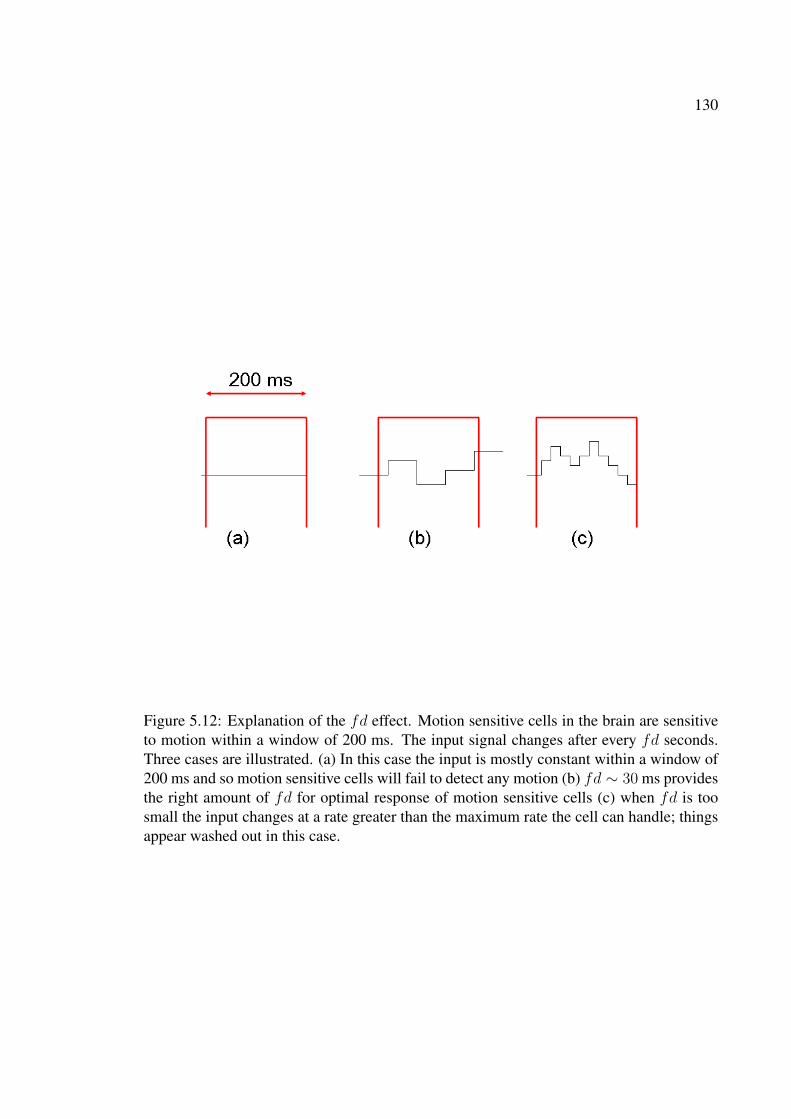
130

Figure 5.12: Explanation of the fd effect. Motion sensitive cells in the brain are sensitiveto motion within a window of 200 ms. The input signal changes after every fd seconds.Three cases are illustrated. (a) In this case the input is mostly constant within a window of200 ms and so motion sensitive cells will fail to detect any motion (b) fd ∼ 30 ms providesthe right amount of fd for optimal response of motion sensitive cells (c) when fd is toosmall the input changes at a rate greater than the maximum rate the cell can handle; thingsappear washed out in this case.

131

I found that the model does show a drop in χ upon changing fd from 30ms to 10ms. It is

interesting to note that without noise χ at fd = 100ms is at the baseline zero level whereas

if noise is added χ rises above zero level and matches value given by human observers.

I found that for the model without noise, in 20 trials only 3 were able to give sufficient

number of LCD crossings to compute χ; for 17 trials of 60s duration each the number of

LCD crossings were less than 2. This shows the beneficial effect noise may sometimes play

in a system.

The ability of the WA model to capture the delicate effects of frame duration on motion

perception is very significant in my opinion. Most motion models especially those used in

computer vision simply do not account for the very important role frame duration plays in

motion perception. They just compute the motion based on two successive frames. As a

consequence the resulting optical flow estimates may not be robust and could be relatively

inaccurate because 2 frames have obviously much less information content than multiple

frames. Why use just 2 frames? Why not use 3 or 4? And how to combine the information

from multiple frames? The answer is that the motion at time t depends on the signal

contained within a window from t − T to t with T ∼ 200 ms so all the frames that fall

within this window need to be considered when computing motion. The number of frames

that fall within this window in turn depends upon the frame duration being used.

132

5.3.6 Effect of dot density dd

Figure 5.13 shows the effect of varying the dot density dd in the display. Humans

display a remarkable indifference to the dot density in the display which goes on to show

it is the relative proportion of the correlated dots that matters not their absolute number. In

chapter 3 I argued how the experimentally observed independence of observer performance

on dot density cannot be explained by models of motion perception based on matching dots

or features to their nearest neighbors in the next frame. Such models display a marked

dependence on dot density in the display according to the probability of mismatch formula

(Williams & Sekuler, 1984) — as the dot density increases there are more dots per unit area

and the chances that the nearest neighbor is not the embedded correlated partner increase.

In reality however observer performance is independent of dot density in the display. The

WA motion detector is able to capture this independence as shown in figure 5.13.

5.3.7 Effect of annulus width ic

The angle subtended by the outer circle diameter is fixed at 10◦ in all our experiments.

Figure 5.14 shows the effect of varying the angle subtended by the inner circle diameter

ic. It is seen that observer performance falls off as the angle subtended by the inner circle

diameter ic is changed from 7◦ to 9.5◦ whereas the model performance remains mostly

unchanged. At ic = 9.5◦ the annulus is very thin and appears like a 1D ring rather than a

2D annulus.

133

0 5 10 15 20 250

0.2

0.4

0.6

0.8

1

dot density (dots/degree2)

χ modelhumans

Figure 5.13: χ vs. dot density dd. c=0.2, ic = 7◦, fd = 30 ms

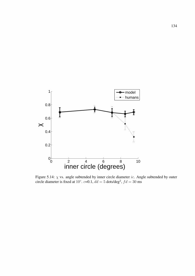
134

0 2 4 6 8 100

0.2

0.4

0.6

0.8

1

inner circle (degrees)

χ

modelhumans

Figure 5.14: χ vs. angle subtended by inner circle diameter ic. Angle subtended by outercircle diameter is fixed at 10◦. c=0.1, dd = 5 dots/deg2, fd = 30 ms

135

5.3.8 Effect of hop size h

The hop size is the amount of displacement given to the correlated dots. By default

the correlated dots are rotated by an angle of 5◦. With ic = 7◦ and angle subtended by

outer circle fixed at 10◦ this translates to average displacement of 7+104× 5 × π

180= 0.37◦

visual angle on the eye. Figures 5.15(a,b) shows the effect of varying the hop size for the

model and humans at different dot densities. The correlated dots were rotated by angles of

{1,5,10,15,20} degrees corresponding to average displacements of {0.074, 0.37, 0.74, 1.11,

1.48} degrees visual angle on the eye. The curves for the model and humans are somewhat

similar; note in particular that changing dot density does not produce any change in χ.

There are some other differences — in particular the -ve values of χ for h = {1.11, 1.48}

degrees for the model suggest a reverse phi motion which is not observed experimentally.

The figures show that as the hop size is increased motion disappears in the display even

though the dot correlation is very high (c = 0.4). This is because if the hop size becomes

greater than the RF size, motion sensitive neurons will fail to register motion. Also impor-

tant is the decrease in χ for human observers if the hop size becomes too small — when an

object moves very slowly it is difficult to discern the motion.

5.3.9 Effect of inserting random frames

Figure 5.16 shows what happens when K random frames are inserted between every

pair of correlated frames. It is seen that observer performance does not fall to zero abruptly

but decreases in a graceful manner showing that the human visual system takes multiples

136

(a)0 0.5 1

0

0.2

0.4

0.6

0.8

1

Hop size (degrees)

χdd=1.3dd=5dd=10

(b)0 0.5 1

−0.2

0

0.2

0.4

0.6

0.8

hop size (degrees)

χ

dd=1.3dd=5dd=10

Figure 5.15: (a) χ vs. hop size for human observers (b) χ vs. hop size for model. c = 0.4,fd = 30 ms, ic = 7◦.

frames into consideration when estimating motion. The model performance also does not

fall to zero abruptly but decreases much more rapidly than human performance. Also it is

to be noted that the model actually predicts reverse phi motion for K={3,4} as reflected by

the -ve values of χ. This shows some of the limitations of the model.

5.3.10 Model Sensitivity to center position

As argued in section 3.3.6 it seems accurate knowledge of position of the true center

relative to which rotation occurs is not needed. Figure 5.17(a) shows model sensitivity to

knowledge of true center position. The rotary motion is computed by the model relative

to a point C that is offset from the true center O. The offset is given by ~OCRi

where Ri is

radius of inner circle. Two curves are shown: in one there is no noise added to the model

i.e. n(t) = 0 and in the other GWN equal to the default value of σ(GWN)/σ0 = 6 is

added to the model. It can be seen that the χ values are not affected much by uncertainty

in knowledge of true center position and start to deteriorate only when the offset becomes

137

0 1 2 3 4−0.2

0

0.2

0.4

0.6

0.8

K

χ

modelhumans

Figure 5.16: Effect of inserting K random frames between correlated frames. c = 0.5,fd = 10 ms, dd = 5 dots/degree2, ic = 7◦.

138

(a)0 0.2 0.4 0.6 0.8 1

0

0.2

0.4

0.6

0.8

1

offset

χ

w/o noisew/ noise

(b)0 0.2 0.4 0.6 0.8 1

0

0.2

0.4

0.6

0.8

1

offset

χ

type1type2

Figure 5.17: χ vs. center relative to which rotary motion is computed. χ values are notaffected much by uncertainty in knowledge of true center position and start to deteriorateonly when the offset becomes very large. This may explain the experimentally observedposition invariance of MST(d) cells. c=0.1, fd = 30 ms, ic = 7◦, dd = 2.5 dots/deg2.(a) full 360◦ of the annulus is visible. (b) only 90◦ of the annulus is made visible; type1— a single 90◦ sector of the racetrack is made visible, type2 — two diametrically oppositelocated sectors each 45◦ in size are made visible

very large. This may explain the experimentally observed position invariance of MST(d)

cells — the fact that the cells are insensitive to where in their RF rotation occurs (Graziano

et al., 1994).

It seems that when only a sector of the racetrack is made visible the condition∑

i ~vi = 0

may not hold true because of the correlated dots. However if two diametrically opposite

located sectors are displayed then∑

i ~vi = 0. Figure 5.17(b) shows χ vs. offset for the

two cases — type1 when only a single 90◦ sector is made visible and type2 when two dia-

metrically opposite located sectors each 45◦ in size are displayed. Interestingly the model

is still robust enough to the offset even when only a sector of the racetrack is displayed

irrespective of whether it is type1 or type2.

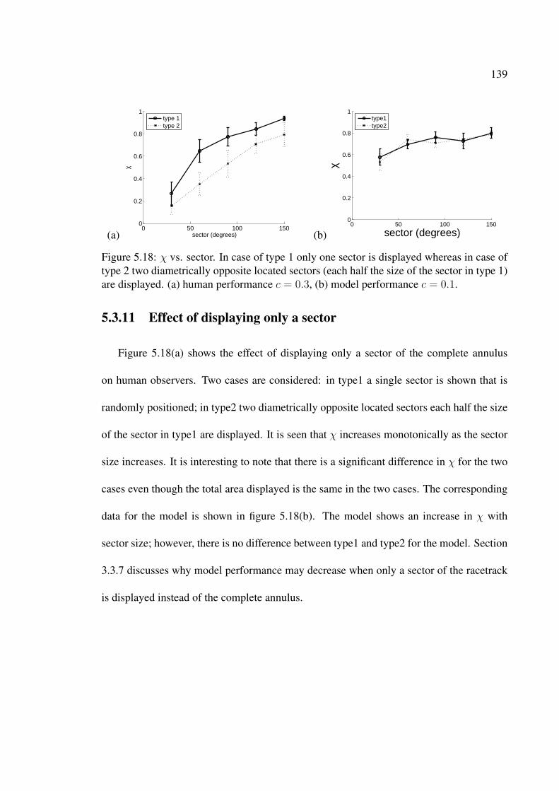
139

(a)0 50 100 150

0

0.2

0.4

0.6

0.8

1

sector (degrees)

χtype 1type 2

(b)0 50 100 150

0

0.2

0.4

0.6

0.8

1

sector (degrees)

χ

type1type2

Figure 5.18: χ vs. sector. In case of type 1 only one sector is displayed whereas in case oftype 2 two diametrically opposite located sectors (each half the size of the sector in type 1)are displayed. (a) human performance c = 0.3, (b) model performance c = 0.1.

5.3.11 Effect of displaying only a sector

Figure 5.18(a) shows the effect of displaying only a sector of the complete annulus

on human observers. Two cases are considered: in type1 a single sector is shown that is

randomly positioned; in type2 two diametrically opposite located sectors each half the size

of the sector in type1 are displayed. It is seen that χ increases monotonically as the sector

size increases. It is interesting to note that there is a significant difference in χ for the two

cases even though the total area displayed is the same in the two cases. The corresponding

data for the model is shown in figure 5.18(b). The model shows an increase in χ with

sector size; however, there is no difference between type1 and type2 for the model. Section

3.3.7 discusses why model performance may decrease when only a sector of the racetrack

is displayed instead of the complete annulus.

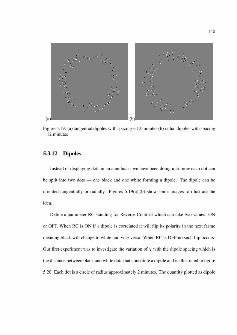
140

(a) (b)

Figure 5.19: (a) tangential dipoles with spacing = 12 minutes (b) radial dipoles with spacing= 12 minutes

5.3.12 Dipoles

Instead of displaying dots in an annulus as we have been doing until now each dot can

be split into two dots — one black and one white forming a dipole. The dipole can be

oriented tangentially or radially. Figures 5.19(a),(b) show some images to illustrate the

idea.

Define a parameter RC standing for Reverse Contrast which can take two values: ON

or OFF. When RC is ON if a dipole is correlated it will flip its polarity in the next frame

meaning black will change to white and vice-versa. When RC is OFF no such flip occurs.

Our first experiment was to investigate the variation of χ with the dipole spacing which is

the distance between black and white dots that constitute a dipole and is illustrated in figure

5.20. Each dot is a circle of radius approximately 2 minutes. The quantity plotted as dipole

141

Figure 5.20: A dipole is formed by two dots — one black and one white. The separationbetween the dots is known as dipole spacing. When the spacing is zero the dots are touchingeach other.

spacing s in the figures in this section is s = d− 2r where d is the center-to-center spacing

and r is radius of a dot. Thus when the dipole spacing is zero the two dots forming a dipole

are touching each other.

It was found that when RC is OFF motion is seen in the normal direction of embedded

motion but when RC is ON several interesting things can happen — at small values of

dipole spacing motion is seen in normal direction but at high values of spacing the motion

flips in the opposite direction. At spacings in between the motion is quite complex — for

the case of tangential dipoles often times the dots near the inner circle seem to moving

142

opposite to the dots near the outer circle; the radial dipoles give a very strong sense of

radial pulsating motion. These results are shown in figure 5.21 which plots χ vs. spacing

for experiment and also compares it to the predictions of the model. Throughout the ex-

periments in this section we will maintain c = 0.5, fd = 30 ms, dd = 2.5, ic = 7◦ and

correlated dipoles will be rotated by an angle of 5◦ in the next frame. In this section we

slightly generalise the definition of χ as follows: let m1, m2 be maximum and minimum

values of the cross correlation function between observer/model response and the input

function. If |m1| > |m2| χ = m1 else χ = m2. In this way when observer is seeing

motion in normal direction χ is +ve whereas when motion is seen in opposite direction χ

is -ve. For the sake of brevity I will focus on the RC ON case exclusively in this section

because that is where most of the novel phenomenon occurs. Following comments are in

order with respect to the experiments of figure 5.21: for the tangential dipole at spacing =

8 there is a feeling of foreground motion which is the motion sensed on casual viewing and

an opposite background motion which is apparent for example if one stares at the center.

Because of these two opposite motions the overall display appears complex and it becomes

hard to unequivocally judge the direction of motion — the situation is very different from

the case of a display in which no rotary motion can be seen; what one feels over here is

that there is rotary motion but because of the foreground/background conflict it is difficult

to say which way it is; motion seems to be seen in both CW and CCW directions simul-

taneously. However with training an observer can learn to attend to either the foreground

or background and discount the other. When this happens an observer can get χ values as

143

(a)0 5 10 15 20

−1

−0.5

0

0.5

1

dipole spacing (minutes)

χtangential dipoleradial dipole

(b)0 5 10 15 20

−1

−0.5

0

0.5

1

dipole spacing (minutes)

χ

tangential dipoleradial dipole

Figure 5.21: (a) χ vs. dipole spacing for experiment r = 1 (b) χ vs. dipole spacing formodel bwir = 1

high as ∼ +1, ∼ −1 depending on whether attention is paid to background or foreground

respectively. This feeling of foreground, background persists for spacing = {12,15} and

the dots at inner circle and outer circle seem to be moving in opposite directions.

From figure 5.21 we note a discrepancy between model and experiment viz. χ is ∼ +1

for experiment whereas it is ∼ −1 for the model at low values of dipole spacing. The

reason for this discrepancy may have to do with the fact that the model simulations were

done with the implicit assumption that the experimental psychophysical conditions were

such that the black and white dots were equally strong perceptually or at least in terms of

their luminance contrast with respect to the gray background. However this assumption is

most likely incorrect. I arbitrarily set the background in above experiments to a gray level

of 150 and set the gray values of black and white dots to 0 and 255 respectively. It is not

at all obvious if this setting corresponds to the condition when the black and white dots are

balanced in terms of their luminance contrast with respect to the gray background. To make

144

this clear let us explicitly define two distinct quantities: the black to white intensity ratio

bwir is a +ve quantity ranging between 0 to +∞ and is equal to the perceptual intensity of

black divided by the perceptual intensity of white which is usually approximated as

I0 − Ib

Iw − I0

(5.9)

where I0, Ib, Iw are the luminance of the background, black and white dots respectively;

whereas let r be defined as

r =150− b

w − 150× 105

150(5.10)

where b, w are the gray levels assigned to black and white respectively while doing ex-

periments. In figure 5.21 the experiments were done by setting r = 1 whereas model

simulations were done by setting bwir = 1. We know that bwir and r are positively cor-

related; however the exact relationship between them is unknown. In particular r = 1 may

not correspond to bwir = 1. Since r = 1 most likely does not imply bwir = 1 it may be

incorrect to compare the model curves with those of the experiment in figure 5.21.

A comparison of model with experiment is however possible in the limiting case: r →

∞ corresponds to bwir →∞ and is the case when the white dots are made invisible. Figure

5.22 shows χ vs. spacing with r = 10 for the experiment and bwir = 10 for the model;

at these values the white dots can be considered to be effectively invisible. Following

observations are in order for the tangential dipole: When spacing = {12,15} minutes the ic

(inner circle) and oc (outer circle) appear to move in opposite directions. The oc moves in

normal direction and ic moves in opposite direction. At spacing=20 minutes one can only

see motion along ic. The χ vs. spacing behavior can be qualitatively understood by the

145

diagrams of figures 5.23, 5.24. For the case of tangential dipole as can be seen from figure

5.23 two types of motion cues occur: in type (a) the black dots are separated by a distance

of h + d, where h is the hop size or the displacement given to the dipole in the next frame

and d is the center-to-center dipole spacing, and in type (b) the black dots are separated by

a distance of h − d. When d > h for type (a) the black dots are separated by such a large

distance that the resulting motion cue is weak and for type (b) the motion cue will reverse

its direction. Since the correlated dipoles are rotated by an angle of θ = 5◦ the hop size

h = rθ depends on the distance r of the dipole from the center; this in turn means that

the spacing at which reversal in motion occurs will be different at ic (inner circle) and oc

(outer circle). This explains the often occuring perception of particles at ic and oc moving

in opposite directions. For the radial dipole figure 5.24 shows the two types of motion cues

that occur. When d becomes comparable to or greater than h the two cues together should

give a perception of radial pulsating motion which is true experimentally. Further as per

figure 5.24 as d increases rotary motion should not really reverse its direction but it should

change into a radial pulsating motion. This is true experimentally — with respect to figure

5.22(a) whereas χ becomes ∼ −1 when spacing=20 minutes for tangential dipole χ drops

to its zero level when spacing=20 minutes for radial dipole.

As per figure 5.21(b) the model predicts a χ value close to −1 at dipole spacing = 1

minute, bwir = 1. As explained earlier since r 6= bwir we cannot expect to see the same

value of χ if experiments are done with r = 1 (cf. χ values of experiment and model in

figure 5.21 at spacing = 1 minute). However since there is a +ve correlation between r and

146

(a)0 5 10 15 20

−1

−0.5

0

0.5

1

dipole spacing (minutes)

χ

tangential dipoleradial dipole

(b)5 10 15 20

−1

−0.5

0

0.5

1

dipole spacing (minutes)

χ

tangential dipoleradial dipole

Figure 5.22: (a) χ vs. dipole spacing for experiment r = 10 (b) χ vs. dipole spacing formodel bwir = 10

bwir is there perhaps some other value of r at which χ ∼ −1 at spacing = 1 minute? To

investigate this experiments were done in which r was varied keeping spacing = 1 minute

and χ values were recorded. Figure 5.25(a) shows the results. As can be seen from the

figure there is a dip in χ at r ≈ 3. For radial dipole χ does drop to about −1 at r ≈ 3.

For the tangential dipole although there is a dip in χ it does not become -ve. Note that

the χ vs. r curve is not symmetric about r = 1; from a symmetry argument we expect

that if a certain value of χ is observed when black is say k times stronger than white then

the same value of χ should occur when white is k times stronger than black. However

remembering once again that r is not the same as bwir it is ok for the χ vs. r curve not

to be symmetric about r = 1. What the symmetry argument suggests is that χ vs. bwir

curve should be approximately symmetrical about bwir = 1. I also ran model simulations

to plot χ vs. bwir at spacing = 1 minute and the results of the simulations are shown in

figure 5.25(b). As can be seen the χ vs. bwir curve does indeed turn out to be symmetrical

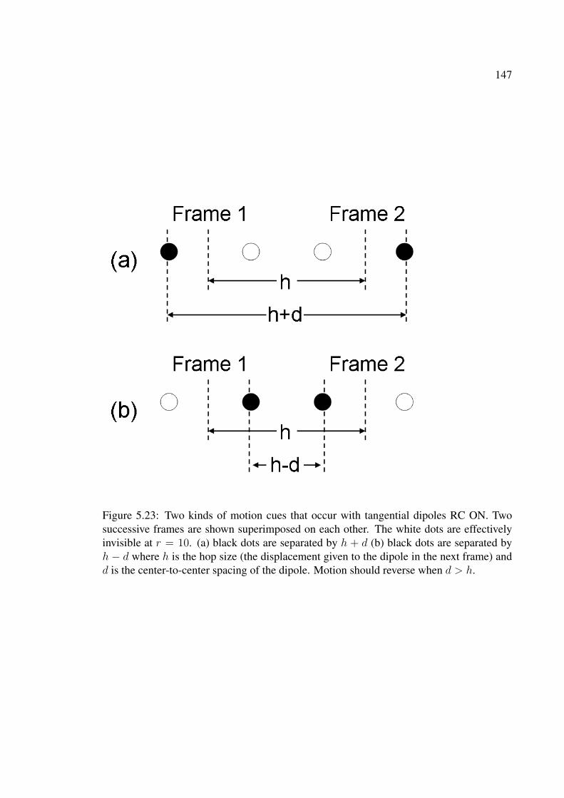
147

Figure 5.23: Two kinds of motion cues that occur with tangential dipoles RC ON. Twosuccessive frames are shown superimposed on each other. The white dots are effectivelyinvisible at r = 10. (a) black dots are separated by h + d (b) black dots are separated byh − d where h is the hop size (the displacement given to the dipole in the next frame) andd is the center-to-center spacing of the dipole. Motion should reverse when d > h.

148

Figure 5.24: Two kinds of motion cues that occur with radial dipoles RC ON. Two succes-sive frames are shown superimposed on each other. The white dots are effectively invisibleat r = 10. h is the hop size (the displacement given to the dipole in the next frame) and d isthe center-to-center spacing of the dipole. When d becomes comparable to or greater thanh these two configurations together should give a sensation of pulsating radial motion.

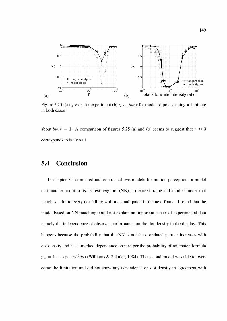
149

(a)10

−110

010

1−1

−0.5

0

0.5

1

r

χ

tangential dipoleradial dipole

(b)10

−110

010

1−1

−0.5

0

0.5

1

black to white intensity ratio

χ

tangential dipoleradial dipole

Figure 5.25: (a) χ vs. r for experiment (b) χ vs. bwir for model. dipole spacing = 1 minutein both cases

about bwir = 1. A comparison of figures 5.25 (a) and (b) seems to suggest that r ≈ 3

corresponds to bwir ≈ 1.

5.4 Conclusion

In chapter 3 I compared and contrasted two models for motion perception: a model

that matches a dot to its nearest neighbor (NN) in the next frame and another model that

matches a dot to every dot falling within a small patch in the next frame. I found that the

model based on NN matching could not explain an important aspect of experimental data

namely the independence of observer performance on the dot density in the display. This

happens because the probability that the NN is not the correlated partner increases with

dot density and has a marked dependence on it as per the probability of mismatch formula

pm = 1− exp(−πh2dd) (Williams & Sekuler, 1984). The second model was able to over-

come the limitation and did not show any dependence on dot density in agreement with

150

human psychophysics but it has two major limitations: 1) it is applicable only to random

dot kinematograms (RDKs) consisting of identical indistinguishable features and requires

a feature extraction step that would detect the positions of the dots, 2) it matches a dot to

other dots only in the next frame i.e. it does a version of NN matching in the temporal

domain; a more accurate model would match a dot to every dot falling within a small spa-

tiotemporal window similar to the RF of a motion sensitive cell. This chapter overcomes

both of these limitations by using the WA motion detector which can be used on any type

of spatiotemporal stimulus not just RDKs. I have found that the WA motion detector can

explain a large portion of psychophysical data concerning visual motion perception such as

the delicate effects of frame duration, observer independence to dot density in the display

and the surprising reverse-phi motion caused by contrast reversing dots making it a realistic

model of human visual motion sensing. Mention should be made here of other models of

motion perception that bear some relationship to the WA motion detector notably (Adelson

& Bergen, 1985; Heeger, 1987; E. Simoncelli & Heeger, 1998). This chapter also investi-

gated the role intrinsic cortical noise may play in visual motion perception. The intrinsic

variability in neural response would manifest itself as uncertainty in motion estimation.

This uncertainty or noise in the generation of response to signals may play an important

role in the perception of motion for low c values (≤ 0.1). The noise (i) can stochastically

boost a weak motion signal so that it becomes large enough to cross a perceptual threshold

for rotary motion, (ii) is also the reason why observers give different responses to the same

stimulus in multiple trials at c = 0. (Fermuller, Pless, & Aloimonos, 2000; Fermuller et

151

al., 2001) have argued that noise in response is the cause of illusory motion perception in

the Ouchi pattern.

152

Chapter 6

THC induced impairment of visual

motion perception

6.1 Introduction

Marijuana or cannabis is a widely used drug for recreational and medicinal purposes

around the world. It can act as a depressant as well as a stimulant. The cannabinoids

— tetrahydrocannabinol (THC), cannabidiol (CBD), cannabinol (CBN) — are the psy-

choactive ingredients of marijuana. ∆9-THC is the main psychomimetic (mindblending)

ingredient of marijuana. It is estimated that 70 to 100% of the marijuana high results

from the ∆9-THC present. It is believed that CBD is not psychomimetic in pure form al-

though it does have sedative, analgesic and antibiotic properties. CBD can contribute to

the marijuana high by interacting with THC to potentiate (enhance) or antagonize (inter-

153

fere or lessen) certain qualities of the high. CBN is not produced by the plant per se. It is

the degradation (oxidative) product of THC. Pure forms of CBN have at most 10% of the

psychoactivity of ∆9-THC.

The metabolism and kinetics of cannabis in humans is well studied and discussed by

(Manno et al., 2001; Huestis, Henningfield, & Cone, 1992a, 1992b; Wall, Sadler, Brine,

Taylor, & Perez-Reyes, 1983; McBurney, Bobbie, & Sepp, 1986) . It is found that THC in

cannabis is rapidly transferred from the lungs to the blood, followed by a rapid decay and

conversion to the active metabolite 11-hydroxy-∆9-THC (11-OH-THC) and the inactive

metabolite 11-Nor-∆9-THC-9-Carboxylic Acid (THCCOOH). There is a strong interest in

trying to understand how THC interacts with the brain and what effects it produces. It is

believed that THC achieves its psychoactivity by acting on the cannabinoid receptor CB1

in the brain. Not only this, the brain itself produces chemicals known as endocannabinoids

(e.g. anandamide and 2AG) that also activate CB1 (Nicoll & Alger, 2004). Marijuana can

cause myriad effects such as hallucinations, sleep, impairing short-term memory, cogni-

tion and motor coordination, alleviating pain and anxiety and enhancing appetite. This is

because the CB1 receptor on which THC acts is found in cerebral cortex, hippocampus, hy-

pothalamus, cerebellum, basal ganglia, brain stem, spinal cord and amygdala among other

places. Marijuana thus acts on numerous targets and in this way produces its many effects.

In this chapter I investigate the effects marijuana has on visual motion perception abil-

ities. Psychophysical experiments were performed on marijuana users with and without

drug in which they were asked to judge the direction of motion in the racetrack stimulus.

154

It is found that THC can cause short term impairment of rotary motion perception abilities

— (a) observer performance decreases by as much as 15%, (b) the reaction time of an ob-

server varies from about 0.8s to about 2s depending upon the strength of motion signal in

the display. Under the influence of drug the reaction time of an observer increases by about

222±96 ms from the baseline.

6.2 Data collection procedures

The study was conducted in collaboration with Dr. Donald Abrams at the San Fran-

cisco General Hospital under compliance of NIH procedures. Participants were adults

aged 21-42yrs (median 26yrs), 10 males 1 female with previous history of THC use. Each

participant enrolled in the hospital for 6 days. On each day s/he took two trials: the first

without drug and the second 15 minutes after drug (marijuana) administration. The drug

dosage on the 6 days was given by a random permutation of the set S = {1.7v, 1.7s, 3.4v,

3.4s, 6.8v, 6.8s}. The numbers {1.7, 3.4, 6.8} reflect % THC by weight and the letters {v,

s} denote the method of drug delivery through vapor or smoke. e.g. patient #970216 was

given 3.4v on day 1, 3.4s on day 2, 1.7s on day 3, 1.7v on day 4, 6.8v on day 5 and 6.8s on

day 6. Each trial consisted of a series of runs starting with c = 0.5 and progressively de-

creasing to c = 0 where c is the fraction of dots that are correlated. The frame duration was

33ms, duration of a run was 2 minutes, total number of dots in the display = 200. Experi-

ments were done in conditions where the lighting and observer distance from screen could

155

not be tightly controlled. At a viewing distance of 1.65m which was the distance given in

instructions to the participants, the outer circle subtended an angle of 10◦ at the eye and the

inner circle subtended an angle of 7◦. This corresponded with a dot density of 5 dots/deg2.

Blood samples of subjects were taken at 2, 30, 60, 180, 360 minutes after drug administra-

tion and the concentration of following five metabolites in the blood were measured using

gas chromatography followed by mass spectroscopy (GC/MS): ∆9-THC, CBD, CBN, 11-

hydroxy-∆9-THC (11-OH-THC), 11-Nor-∆9-THC-9-Carboxylic Acid (THCCOOH).

6.3 Results

6.3.1 Timecourse of metabolites & effect of THC on observer perfor-

mance

Figures 6.1-6.5 show the timecourse of decay of various metabolites in the blood after

drug administration. Note that the concentration of ∆9 THC is much higher than that of

other metabolites, THC being the main active ingredient in marijuana. Consistent with

earlier studies, it is found that ∆9 THC is rapidly transferred to the blood plasma from the

lungs with concentration peaking as soon as 2 minutes after drug administration followed

by rapid decay in blood plasma. At t = 180 minutes post drug administration the mean

concentration is 3.5ng/ml. The rapid decay of THC in blood plasma is attributed to the

highly lipophilic nature of THC resulting in rapid distribution from blood to the tissues, and

to its rapid conversion to more polar (hydrophilic) metabolites (Wall et al., 1983). Figures

156

Dosage level mean (vapor) s.e.m. (vapor) mean (smoke) s.e.m. (smoke) t-statistic P value1.7 58.43 10.01 61.45 18.53 -0.23 0.823.4 108.16 17.22 144.68 21.72 -1.32 0.206.8 180.85 64.46 142.89 24.61 0.55 0.58

Table 6.1: Mean, s.e.m., t-statistic and P value for THC concentration (ng/ml) under vaporand smoke. The P value is the probability of observing the observed difference in meansor even more extreme by chance assuming the null hypothesis is true — that there is nodifference in the concentration of THC delivered by vapor and smoke. Small values of Pcast doubt on the validity of the null hypothesis.

6.2, 6.3 show the rapid decay of CBD and CBN the other cannabinoids found in marijuana.

The metabolism of ∆9THC leads to the appearance of the active metabolite 11-hydroxy-

∆9-THC (11-OH-THC) and the inactive metabolite 11-Nor-∆9-THC-9-Carboxylic Acid

(THCCOOH). Their slow decay is shown in figures 6.4, 6.5. THCCOOH in particular is

characterized by a very slow decay and eventually can still be detected in the blood when no

traces of THC can be detected. Table 6.1 lists the mean, s.e.m. of THC concentration under

vapor and smoke and for the 3 dosage levels at t = 2 minutes post smoking. The table also

lists the t-statistic and P value to test whether there is any appreciable difference in THC

concentration under vapor or smoke. Vapor and smoke appear to be equally effective as a

drug delivery medium.

Figure 6.6 shows a plot of χ the observer performance vs. c the dot correlation for

different doses of the drug. A χ value of 1 implies perfect detection of the embedded motion

in the stimulus. At c = 0 there are no correlated dots in the stimulus and thus the input

function does not have any physical significance; the χ value however is not zero because

χ is the maximum of the cross correlation function between the observer response and

the input function. It is seen from the graph that as the dot correlation increases observer

157

0 100 200 3000

50

100

150

200

250

time (minutes)

conc

entr

atio

n (n

g/m

l)

∆9 THC

1.7v1.7s3.4v3.4s6.8v6.8s

Figure 6.1: Timecourse of ∆9 THC in blood plasma. Data from 11 subjects. Errorbars are± s.e.m.

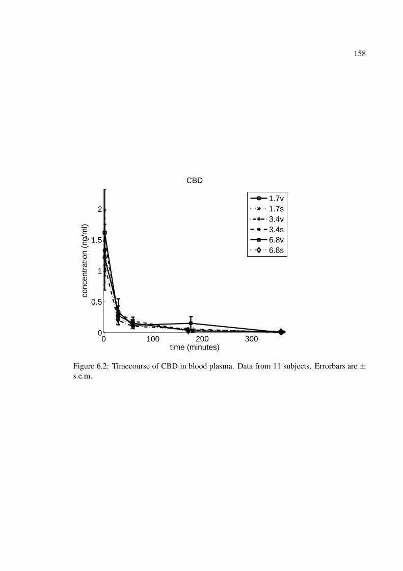
158

0 100 200 3000

0.5

1

1.5

2

time (minutes)

conc

entr

atio

n (n

g/m

l)

CBD

1.7v1.7s3.4v3.4s6.8v6.8s

Figure 6.2: Timecourse of CBD in blood plasma. Data from 11 subjects. Errorbars are ±s.e.m.

159

0 100 200 3000

2

4

6

8

10

time (minutes)

conc

entr

atio

n (n

g/m

l)

CBN

1.7v1.7s3.4v3.4s6.8v6.8s

Figure 6.3: Timecourse of CBN in blood plasma. Data from 11 subjects. Errorbars are ±s.e.m.

160

0 100 200 3000

2

4

6

8

10

time (minutes)

conc

entr

atio

n (n

g/m

l)

11−OH−THC

1.7v1.7s3.4v3.4s6.8v6.8s

Figure 6.4: Timecourse of 11-OH-THC in blood plasma. Data from 11 subjects. Errorbarsare ± s.e.m.

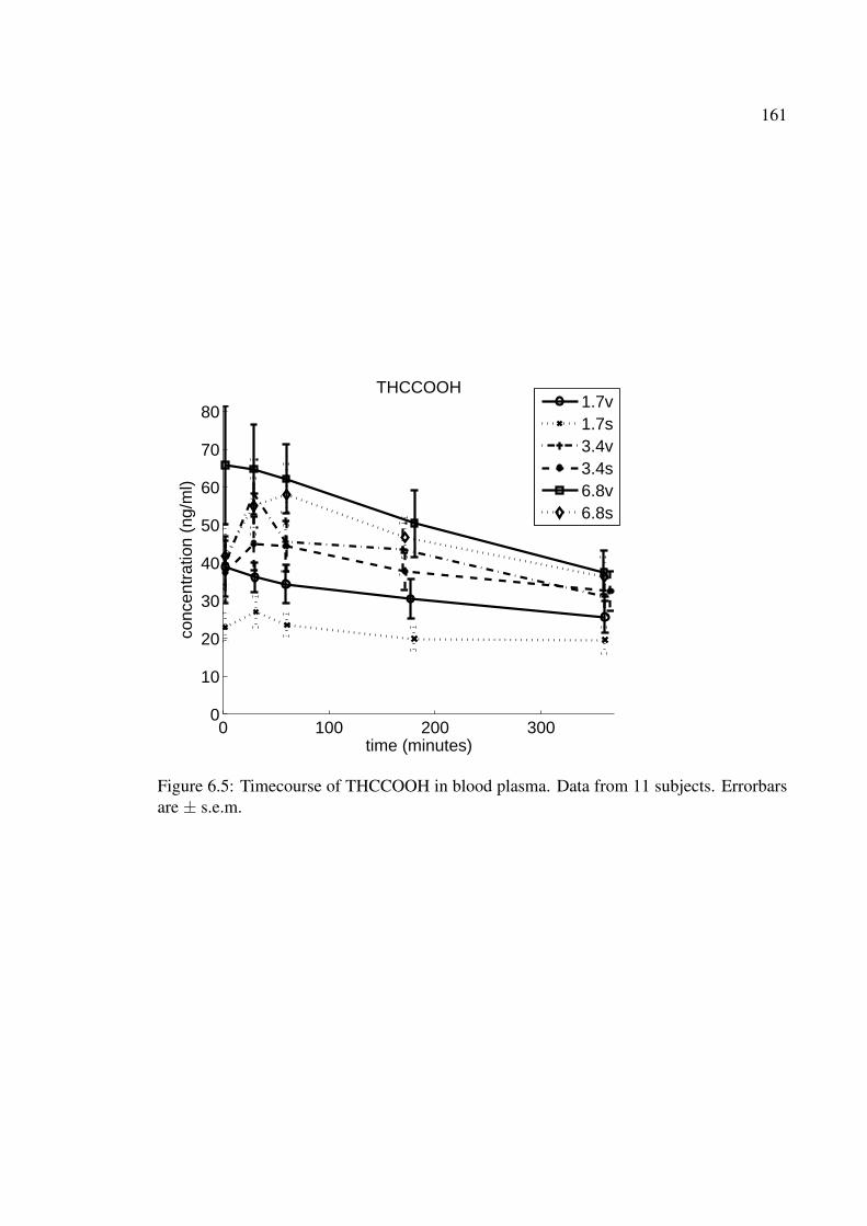
161

0 100 200 3000

10

20

30

40

50

60

70

80

time (minutes)

conc

entr

atio

n (n

g/m

l)

THCCOOH1.7v1.7s3.4v3.4s6.8v6.8s

Figure 6.5: Timecourse of THCCOOH in blood plasma. Data from 11 subjects. Errorbarsare ± s.e.m.

162

0 0.1 0.2 0.3 0.4 0.50

0.1

0.2

0.3

0.4

0.5

0.6

0.7

0.8

0.9

1

dot correlation

χ01.7v1.7s3.4v3.4s6.8v6.8s

Figure 6.6: Plot of χ vs. c. Data from 11 subjects. The numbers {0, 1.7, 3.4, 6.8} indicate% THC administered. The letters {v, s} indicate the method of drug delivery — throughvapor or smoke. Errorbars are ± s.e.m.

performance also increases. The drug does have a measureable effect as all the drug curves

are below the curve without drug. This is further made clearer in figure 6.7 which shows

the data under two cases — with and without drug. The effect of drug is most pronounced

at c=0.20 where χ drops from about 0.70 to 0.55, a decrease of about 15%.1

To examine the effect of drug dosage, figure 6.8 shows the data of figure 6.6 but with

the vapor and smoke combined. There is significant overlap among the curves for 3.4%

and 6.8% THC. At c = {0.1, 0.4} the χ value is actually higher for 6.8% THC than for

1In figures 6.6-6.7 the χ value at c = 0.4 is higher than the χ value at c = 0.5. This reason for thisanomalous result may be that the subjects started the experiments with c = 0.5 and progressively decreasedthe c values to c = 0. c = 0.5 was the first run done by the subjects.

163

0 0.1 0.2 0.3 0.4 0.50

0.1

0.2

0.3

0.4

0.5

0.6

0.7

0.8

0.9

1

dot correlation

χ

w/o drugw/ drug

Figure 6.7: Plot of χ vs. c with and without drug. Data from 11 subjects. Errorbars are ±s.e.m.

164

0 0.1 0.2 0.3 0.4 0.50

0.1

0.2

0.3

0.4

0.5

0.6

0.7

0.8

0.9

1

dot correlation

χ

w/o drug1.73.46.8

Figure 6.8: Plot of χ vs. c. Data from 11 subjects. The numbers {0, 1.7, 3.4, 6.8} indicate% THC administered. Errorbars are ± s.e.m.

165

0 0.1 0.2 0.3 0.4 0.50

0.1

0.2

0.3

0.4

0.5

0.6

0.7

0.8

0.9

1

dot correlation

χ

w/o drugvaporsmoke

Figure 6.9: Plot of χ vs. c. Data from 11 subjects. The letters {v, s} indicate the method ofdrug delivery — through vapor or smoke. Errorbars are ± s.e.m.

166

c 0.1 0.2 0.3 0.4τ1 1.7460 1.3064 0.9250 0.7740τ2 2.1103 1.4643 1.1024 0.9620

d = τ2 − τ1 .3643 .1579 .1774 .1880

Table 6.2: τ1 is reaction time (in seconds) without drug and τ2 is reaction time (in seconds)under the influence of drug. Mean(d) = 0.222s, std(d) = 0.0957s.

3.4% THC. At c = {0.2, 0.3} the χ values for 3.4% and 6.8% THC are nearly the same.

Figure 6.9 shows the data of figure 6.6 with the different dosage levels combined but the

smoke and vapor separated out. Vapor and smoke appear equally effective in producing the

motion impairment.

Figure 6.10 shows τ the reaction time vs. c with and without drug. The reaction time

of an observer varies from about 0.8s to about 2s depending upon the strength of motion

signal in the display. Under the influence of drug the reaction time of an observer increases

by about 222±96 ms from the baseline as calculated in table 6.2.

Each run of the racetrack gives us two numbers χ and τ . These two quantities are

inversely correlated as shown by figure 6.11. When observer performance is good it takes

less time to recognize the motion and when observer performance is bad it takes more time

to recognize the motion. There is no difference in the τ vs. χ curve with and without drug.

6.3.2 Building a classifier to detect drug use

To further quantify the extent to which THC impairs motion perception suppose it is

desired to find out whether a person is drugged or not based on a single run of the racetrack.

From figure 6.7 the effect of drug is most pronounced for c = 0.20 so it is best to ask the

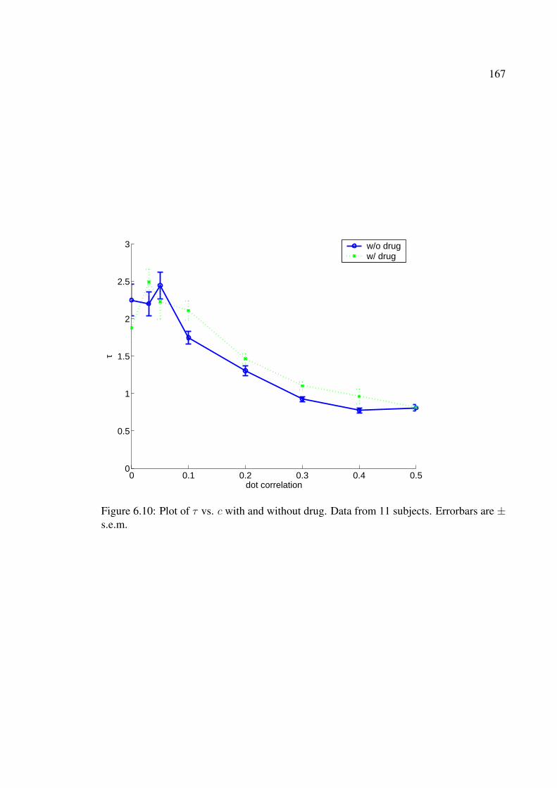
167

0 0.1 0.2 0.3 0.4 0.50

0.5

1

1.5

2

2.5

3

dot correlation

τ

w/o drugw/ drug

Figure 6.10: Plot of τ vs. c with and without drug. Data from 11 subjects. Errorbars are ±s.e.m.

168

0 0.2 0.4 0.6 0.8 10

0.5

1

1.5

2

2.5

3

χ

τ (s

)

w/o drugw/ drug

Figure 6.11: Plot of τ vs. χ. Data from 11 subjects. Errorbars are ± s.e.m.

169

subject to take the run at c = 0.20. Using standard decision analysis a classifier is built

with following decision rule: if χ given by subject is less than ρ classify as drugged else

classify as non-drugged. The probability of error of the classifier is given by

e = P (classify as drugged|subject is not drugged)P (subject is not drugged)

+ P (classify as non-drugged|subject is drugged)P (subject is drugged)

(6.1)

where P (subject is not drugged) = P (subject is drugged) = 0.5 in our case. This gives

e =1

2(1− F1(ρ) + F2(ρ)) (6.2)

where F1 is the cdf (cumulative distribution function) of χ under the hypothesis H1 that

subject is drugged and F2 is the cdf of χ under the hypothesis H2 that subject is not drugged.

The optimal ρ denoted by ρ∗ would minimize e giving

f1(ρ∗) = f2(ρ

∗) (6.3)

where f1 and f2 are the pdfs under the hypotheses H1 and H2 respectively. If following

two conditions hold:

f1(µ1 + x) = f2(µ2 + x) (6.4)

f1(µ1 + x) = f1(µ1 − x) (6.5)

where µ1 = mean(χ) under hypothesis H1 and µ2 = mean(χ) under hypothesis H2 then

ρ∗ is given by the simple formula

ρ∗ =µ1 + µ2

2(6.6)

170

From figure 6.7 at c = 0.2

µ1s = 0.5504 σ1s = 0.2024 sample mean and S.D. ofχunder hypothesisH1 (6.7)

µ2s = 0.7054 σ2s = 0.1774 sample mean and S.D. ofχunder hypothesisH2 (6.8)

If we assume that χ is normally distributed and approximate

µ1 = µ1s µ2 = µ2s σ1 = σ2 =σ1s + σ2s

2(6.9)

where σ1 and σ2 are the standard deviation (S.D.) of χ under the hypotheses H1 and H2

respectively then from equation 6.2 we find that e = 0.34.

The actual classification results on the data using such a classifier are summarized by

the following confusion matrix:

C =

45/63 18/63

25/63 38/63

=

0.71 0.29

0.40 0.60

(6.10)

where the meaning of various entries is as follows: 45 cases when subject was not drugged

were correctly classified, 18 cases when subject was not drugged were incorrectly classi-

fied, 25 cases when subject was drugged were incorrectly classified, and 38 cases when

subject was drugged were correctly classified. This gives e = 0.34.

In summary a classifier to detect whether a patient is drugged or not based on a single

racetrack run can be expected to be wrong about 1/3rd of the time and therefore of little

practical use.

171

6.4 Conclusion

This chapter demonstrates that there is a measurable effect of THC on motion percep-

tion: observer performance decreases by as much as 15% and the reaction time increases

by 222±96 ms from a baseline of 0.8s-2s depending on the strength of motion in the dis-

play. I suspect that the effects of THC would be even more pronounced on subjects without

any history of prior THC use. The mechanism by which THC affects motion perception is

debatable: is the drop in performance under influence of THC simply because of lack of

motivation or does THC interact with the neurotransmitters that influence motion process-

ing in the brain? This may be resolved in conjunction with fMRI studies which may be

used to determine the targets where THC acts in the brain. (Rizzo et al., 2005) write “Ne-

fazodone, an antidepressant that inhibits serotonin reuptake and blocks 5-HT2 receptors,

may cause a transient defect of visual motion perception (Horton and Trobe 1999)...” They

further argue that THC users show an impairment at the heading task but do not show any

impairment at the structure from motion task.2 The former requires pooling information

over an extended area of the display while the latter task is performed by comparisons of

local neighborhood velocities. In our case, determining the direction of rotary motion also

requires pooling of information over an extended area of display. However, determining the

direction of motion in stochastic translational motion displays supposedly does not require

such pooling and is directly given by the local motion. Does that mean THC users will

2Note that (Rizzo et al., 2005) have done their experiments on THC users who are asked to abstain fromdrug use on the day of testing whereas in our study the participant was given drug at the time of experiment.

172

not show any impairment on displays such as those of (Newsome & Pare, 1988; Williams

& Sekuler, 1984)? Psychopharmacological studies like this are also valuable in designing

new tests to determine drug intoxication e.g. see (Kosnoski, Yolton, Citek, Hayes, & Evans,

1998).

6.5 Acknowledgements

I wish to thank Dr. Donald Abrams and his talented team at UCSF without whose help

this study would not have been possible. Thanks are due to Hector Visozo who promptly

answered many of my queries and provided me the data on metabolite concentrations.

173

Chapter 7

Conclusion

The goal of the research described in this dissertation was to understand the mecha-

nisms by which the brain senses motion. The major contributions of the dissertation are as

follows:

• The dissertation describes a detailed psychophysical characterisation of visual mo-

tion perception in general and the peculiar omega effect originally discovered by

Rose & Blake in particular in which dynamic random noise in the form of random

dots displayed in a circular annulus evokes the illusion of rotary motion. Observer

performance and reaction time are measured against a variety of psychophysical pa-

rameters such as dot correlation, frame duration, dot density, annulus width, hop size,

reverse contrast and so on.

• I find that a model based on the Watson & Ahumada (WA) motion detector is able to

explain most and key parts of the psychophysical data such as the very delicate effects

174

of frame duration on motion perception, independence of observer performance on

dot density in the display and the surprising reverse phi motion caused by contrast

reversing dots. In addition to explaining the psychophysical data, the model relates

reasonably well to what is known about the neurobiology of motion sensitive cells

in the brain making it a realistic model of human visual motion sensing. (Mante

& Carandini, 2003) have recently used the WA framework to explain the optical

imaging results of (Basole, White, & Fitzpatrick, 2003).

• Experiments have also been done on observers under the influence of marijuana and

it is found that the THC in marijuana can cause an impairment of motion perception

abilities — observer performance decreases by as much as 15% and reaction time

increases by as much as 222±96 ms.

Some other highlights of the dissertation are as follows:

• For the c = 0 case which has been of some special interest to us it is found that

although the display triggers perception of rotary motion, an observer gives different

responses to the same stimulus in multiple trials. This finding means the motion sig-

nal if any in the stimulus itself at c = 0 is so weak as to be undetectable by human

observers and supports the hypothesis that the phenomenon is dominated by internal

mechanisms such as the intrinsic cortical noise in the brain. On closer inspection it

is realised that displaying dots in a circular annulus restricts their freedom of move-

ment — the dots at the boundary cannot move in all 360◦ directions. In the limit

175

when the annulus width is made vanishingly small the dots will only be able to move

tangentially. This suggests that the omega effect should vanish for a thick annulus

and become more pronounced for a thin annulus which is experimentally true.

A few qualitative observations at c = 0 are as follows: (i) after prolonged viewing

observers can usually will the direction of motion in the display (ii) the direction

of motion reverses whenever an attention grabbing stimulus, active or passive, is

presented to an observer (iii) the rotation reversals in the racetrack are more or less

instantaneous upon willing or when an external attention grabbing stimulus such as

a tap at the back of the forehead is given; however rotation reversals in other bistable

stimuli such as the Necker cube are not instantaneous and take a few seconds to

occur. This could be because the 3D perception of Necker cube depends on higher

areas in the brain involving shape and depth perception whereas the rotary motion

perception at c = 0 in the racetrack does not depend on such processes.

• It is postulated that the intrinsic cortical noise in the brain will manifest itself as

uncertainty in motion estimation. I find that this noise can play an important role

in perception by significantly improving detectability of subliminal motion cues at

the expense of a very modest drop in performance for a suprathreshold signal ala

stochastic resonance.

• I find that the observer performance is invariant to dot density in the display and argue

that this provides very powerful evidence against motion models based on matching

176

dots to nearest neighbors in successive frames ala (Ullman, 1979; Dawson, 1991)

etc.

• I find and prove that the rotary motion signal does not depend on the center of rotation

relative to which it is computed which explains the experimentally observed position

invariance of MST(d) cells found by (Graziano et al., 1994).

A few open questions at this point are as follows:

• Performance testing of the WA model on real-world imagery, e.g. the Yosemite se-

quence, the Hamburg taxi sequence and other real and synthetic test cases that are

used to compare performance of optical flow algorithms in computer vision litera-

ture, has not been done.

• To my knowledge little is known about the mechanisms by which illusory motion

is seen in some static images such as Leviant’s Enigma and Kitaoka’s snakes. Most

visual illusions are characterised by the fact that they have a very high degree of

geometrical structure to them. Why are such patterns effective at generating illusory

percepts?

177

References

Adelson, E. H., & Bergen, J. R. (1985). Spatiotemporal energy models for the perception

of motion. Journal of Optical Society of America, A, 2(2), 284–299.

Albright, T. D., & Desimone, R. (1987). Local precision of visuotopic in the middle

temporal area (MT) of the macaque. Experimental Brain Research, 65, 582–592.

Anstis, S. M. (1980). The perception of apparent movement. Philosophical Transactions

of the Royal Society of London. Series B, Biological Sciences, 290, 153–168.

Anstis, S. M., & Rogers, B. J. (1975). Illusory reversal of visual depth and movement

during changes of contrast. Vision Research, 15, 957–961.

Baker, S., & Matthews, I. (2004). Lucas-kanade 20 years on: A unifying framework.

International Journal of Computer Vision, 56, 221–225.

Barlow, H., & Tripathy, S. P. (1997). Correspondence noise and signal pooling in the

detection of coherent visual motion. Journal of Neuroscience, 17(20), 7954–7966.

Barron, J. L., & Beauchemin, S. S. (1995). The computation of optical flow. ACM Com-

puting Surveys, 27(8), 433–467.

Barron, J. L., Fleet, D. J., Beauchemin, S. S., & Burkitt, T. A. (1992). Performance of

178

optical flow techniques. IEEE Computer Vision and Pattern Recognition, 236–242.

Basole, A., White, L. E., & Fitzpatrick, D. (2003). Mapping multiple features in the

population response of visual cortex. Nature, 423, 986–990.

Benzi, R., Sutera, A., & Vulpani, A. (1981). The mechanism of stochastic resonance. J.

Phys A, 14, L453–7.

Born, R. T., & Bradley, D. C. (2005). Structure and function of visual area MT. Annual

Reviews Neuroscience, 28, 157–189.

Brox, T., Bruhn, A., Papenberg, N., & Weickert, J. (2004). High accuracy optical flow

estimation based on a theory for warping. European Conference on Computer Vision,

25–36.

Bruhn, A., Weickert, J., & Schnorr, C. (2005). Lucas/kanade meets horn/shunck: Combin-

ing local and global optic flow methods. International Journal of Computer Vision,

61(3), 211–231.

Camus, T. (1997). Real-time quantized optical flow. Journal of Real-Time Imaging (special

issue on Real-Time Motion Analysis), 3, 71–86.

Cavanagh, P. (1991). Short-range vs. long-range motion: Not a valid distinction. Spatial

Vision, 5, 303–309.

Dawson, M. R. W. (1991). The how and why of what went where in apparent motion:

Modeling solutions to the motion correspondence problem. Psychological Review,

98(4), 569–603.

DeAngelis, G. C., Ohzawa, I., & Freeman, R. D. (1993). Spatiotemporal organization

179

of simple-cell receptive fields in the cats striate cortex. i. general characteristics and

postnatal development. Journal of Neurophysiology, 69(4), 1091–1117.

DeAngelis, G. C., Ohzawa, I., & Freeman, R. D. (1995). Receptive-field dynamics in the

central visual pathways. Trends in Neuroscience, 18(10), 451–458.

DeAngelis, G. C., Ohzawa, I., & Freeman, R. D. (1996). Reply to TINS letter

to the Editor by Wang et. al. Trends in Neuroscience, 19, 386. (Also avail-

able as http://neurovision.berkeley.edu/other/commentaries/

Letters/ReplyWangTINS96.html)

Derrington, A. M., Allen, H. A., & Delicato, L. S. (2004). Visual mechanisms of motion

analysis and motion perception. Annual Reviews Psychology, 55, 181–205.

Duffy, C. J., & Wurtz, R. H. (1995). Response of monkey MST neurons to optic flow

stimuli with shifted centers of motion. Journal of Neuroscience, 15(7), 5192–5208.

Duffy, C. J., & Wurtz, R. H. (1997). Planar directional contributions to optic flow responses

in MST neurons. Journal of Neurophysiology, 77(2), 782–796.

Felleman, D. J., & Kaas, J. H. (1984). Receptive-field properties of neurons in middle

temporal visual area (MT) of owl monkeys. Journal of Neurophysiology, 52(3),

488–513.

Fermuller, C., Pless, R., & Aloimonos, Y. (2000). The ouchi illusion as an artifact of biased

flow estimation. Vision Research, 40(1), 77–96.

Fermuller, C., Shulman, D., & Aloimonos, Y. (2001). The statistics of optical flow. Com-

puter Vision and Image Understanding, 82, 1–32.

180

Galvin, B., McCane, B., Novins, K., Mason, D., & Mills, S. (1998). Recovering mo-

tion fields: An evaluation of eight optical flow algorithms. British Machine Vision

Conference, 1, 195–204.

Gammaitoni, L., Hanggi, P., Jung, P., & Marchesoni, F. (1998). Stochastic resonance.

Reviews of Modern Physics, 70(1), 223–287.

Gingl, Z., Kiss, L. B., & Moss, F. (1995). Non-dynamical stochastic resonance: Theory and

experiments with white and various colored noises. Nuovo Cimento, 17D, 795–802.

Graziano, M. S. A., Andersen, R. A., & Snowden, R. J. (1994). Tuning of mst neurons to

spiral motions. Journal of Neuroscience, 14(1), 54–67.

Grzywacz, N. M., & Merwine, D. K. (2003). Neural basis of motion perception. Encyclo-

pedia of Cognitive Science, 3, 86–98.

Grzywacz, N. M., Watamaniuk, S. N. J., & McKee, S. P. (1995). Temporal coherence

theory for the detection and measurement of visual motion. Vision Research, 35(22),

3183–3203.

Heeger, D. J. (1987). Model for the extraction of image flow. Journal of Optical Society

of America, A, 4(8), 1455–1471.

Horn, B. K. P., & Shunck, B. (1981). Determining optical flow. Artificial Intelligence, 17,

185–203.

Huestis, M., Henningfield, J., & Cone, E. (1992a). Blood cannabinoids i. absorption of thc

and formation of 11-oh-thc and thccooh during and after smoking marijuana. Journal

of Analytical Toxicology, 16, 276–282.

181

Huestis, M., Henningfield, J., & Cone, E. (1992b). Blood cannabinoids ii. models

for the prediction of time of marijuana exposure from plasma concentrations of

δ9-tetrahydrocannabinol (thc) and 11-nor-9-carboxy-δ9-tetrahydrocannabinol (thc-

cooh). Journal of Analytical Toxicology, 16, 283–290.

Irani, M. (1999). Multi-frame optical flow estimation. IEEE International Conference on

Computer Vision, 1, 626–633.

Kitajo, K., Nozaki, D., M.Ward, L., & Yamamoto, Y. (2003). Behavioral stochastic reso-

nance within the human brain. Physical Review Letters, 90(21), 218103.

Koch, C. (2006). Biological models of motion perception: Spatio-temporal energy models

and electrophysiology. (Lecture Notes for CNS186. available as http://www.

klab.caltech.edu/cns186/cns186-motion-2.pdf)

Kolers, P. A. (1972). Aspects of Apparent Motion. Pergamon, New York.

Kosnoski, E., Yolton, R., Citek, K., Hayes, C., & Evans, R. (1998). The drug evaluation

classification program: using ocular and other signs to detect drug intoxication. J.

Am. Optom. Assoc., 69(4), 211–227.

Kumar, T., & Glaser, D. A. (2006). Illusory motion in enigma: A psychophysical investi-

gation. PNAS, 103(6), 1947–1952.

Limpert, E., Stahel, W. A., & Abbt, M. (2001). Lognormal distributions across the sciences:

Keys and clues. BioScience, 341–352.

Lucas, B. D., & Kanade, T. (1981). An iterative image registration technique with an

application to stereo vision. Proceedings of Image Understanding Workshop, 121–

182

130.

MacKay, D. M. (1965). Visual noise as a tool of research. Journal of General Psychology,

181–197.

Manno, J., Manno, B., Kemp, P., Alford, D., Abukhalaf, I., McWilliams, M., et

al. (2001, October). Temporal indication of marijuana use can be estimated

from plasma and urine concentrations of δ9-tetrahydrocannabinol, 11-hydroxy-δ9-

tetrahydrocannabinol, and 11-nor-δ9-tetrahydrocannabinol-9-carboxylic acid. Jour-

nal of Analytical Toxicology, 25, 538–549.

Mante, V., & Carandini, M. (2003, December). Visual cortex: Seeing motion. Current

Biology, 13, 906–908.

Maunsell, J. H., & Van Essen, D. C. (1981a). Functional properties of neurons in middle

temporal visual area of the macaque monkey. II. binocular interactions and sensitivity

to binocular disparity. Journal of Neurophysiology, 49(5), 1148–1167.

Maunsell, J. H., & Van Essen, D. C. (1981b). Functional properties of neurons in middle

temporal visual area of the macaque monkey. I. selectivity for stimulus direction,

speed, and orientation. Journal of Neurophysiology, 49(5), 1127–1147.

McBurney, L., Bobbie, B., & Sepp, L. (1986). Gc/ms and emit analysis for δ9-

tetrahydrocannabinol metabolites in plasma and urine of human subjects. Journal

of Analytical Toxicology, 10, 56–63.

McCane, B., Novins, K., Crannitch, D., & Galvin, B. (2001). On benchmarking optical

flow. Computer Vision and Image Understanding, 84, 126–143.

183

Morgan, M. J. (1980). Analogue models of motion perception. Philosophical Transactions

of the Royal Society of London. Series B, Biological Sciences, 290(1038), 117–135.

Mori, T., & Kai, S. (2002). Noise-induced entrainment and stochastic resonance in human

brain waves. Physical Review Letters, 88(21), 218101.

Moss, F., Ward, L. M., & Sannita, W. G. (2004). Stochastic resonance and sensory infor-

mation processing: a tutorial and review of application. Clinical Neurophysiology,

115, 267–281.

Newsome, W., Britten, K., & Movshon, J. (1989, September). Neuronal correlates of a

perceptual decision. Nature, 341(6237), 52–54.

Newsome, W., & Pare, E. (1988, June). A selective impairment of motion perception

following lesions of the middle temporal visual area (MT). Journal of Neuroscience,

8(6), 2201–2211.

Nicoll, R. A., & Alger, B. E. (2004). The brain’s own marijuana. Scientific American,

291(6), 69–75.

Riani, M., & Simonotto, E. (1994, May). Stochastic resonance in the perceptual inter-

pretation of ambiguous figures: A neural network model. Physical Review Letters,

72(19), 3120–3123.

Rizzo, M., Lamers, C., Sauer, C., Ramaekers, J., Bechara, A., & Andersen, G. (2005,

May). Impaired perception of self-motion (heading) in abstinent ecstasy and mari-

juana users. Psychopharmacology, 179(3), 559–566.

Rose, D., & Blake, R. (1998). Motion perception: From phi to omega. Philosophical

184

Transactions: Biological Sciences, 353(1371), 967–980.

Ross, J., Badcock, D. R., & Hayes, A. (2000). Coherent global motion in the absence of

coherent velocity signals. Current Biology, 10, 679–682.

Ross, J., & Burr, D. (1983). The psychophysics of motion. In M. A. Arbib & A. R. Hanson

(Eds.), Proceedings of the workshop of vision, brain and cooperative computation.

U. Massachusetts Press, Amherst.

Roth, S., & Black, M. J. (2005). On the spatial statistics of optical flow. IEEE International

Conference on Computer Vision, 1, 42–49.

Rust, N. C., Mante, V., Simoncelli, E. P., & Movshon, J. A. (2006). How mt cells analyze

the motion of visual patterns. Nature Neuroscience, 9(11), 1421–1431.

Sakata, H., Shibutani, H., Ito, Y., Tsurugai, K., Mine, S., & Kusunoki, M. (1994). Func-

tional properties of rotation-sensitive neurons in the posterior parietal association

cortex of the monkey. Experimental Brain Research, 101(2), 183–202.

Salzman, C. D., Britten, K. H., & Newsome, W. T. (1990). Cortical microstimulation

influences perceptual judgements of motion direction. Nature, 346, 174–177.

Salzman, C. D., Murasugi, C. M., Britten, K. H., & Newsome, W. T. (1992). Microstimula-

tion in visual area MT: effects on direction and discrimination performance. Journal

of Neuroscience, 6, 2331–2355.

Santen, J. P. H. van, & Sperling, G. (1985). Elaborated reichardt detectors. Journal of

Optical Society of America, A, 2(2), 300–321.

Scase, M. O., Braddick, O. J., & Raymond, J. E. (1996). What is noise for the motion

185

system? Vision Research, 36(16), 2579–2586.

Shafique, K., & Shah, M. (2005). A non-iterative greedy algorithm for multiframe point

correspondence. IEEE Pattern Analysis and Machine Intelligence, 27(1), 1–15.

Simoncelli, E., & Heeger, D. J. (1998). A model of neuronal responses in visual area MT.

Vision Research, 38(5), 743–761.

Simoncelli, E. P. (1993). Distributed representation and analysis of visual motion. PhD

dissertation, MIT.

Simonotto, E., Riani, M., Seife, C., Roberts, M., Twitty, J., & Moss, F. (1997). Visual

perception of stochastic resonance. Physical Review Letters, 78(6), 1186–1189.

Sincich, L. C., Park, K. F., Wohlgemuth, M. J., & Horton, J. C. (2004). Bypassing V1: a

direct geniculate input to area MT. Nature Neuroscience, 7(10), 1123–1128.

Snowden, R. J. (1994). Visual detection of motion. In A. T. Smith & R. J. Snowden (Eds.),

(pp. 51–83). Academic Press.

Sperling, G. (1976). Movement perception in computer-driven visual displays. Behav. Res.

Methods Instrum., 8, 144–151.

Stiller, C., & Konrad, J. (1999). Estimating motion in image sequences. IEEE Signal

Processing Magazine, 16, 70–91.

Tanaka, K., & Saito, H.-A. (1989). Analysis of motion of the visual field by direction,

expansion/contraction, and rotation cells clustered in the dorsal part of the medial

superior temporal area of the macaque monkey. Journal of Neurophysiology, 62(3),

626–641.

186

Ullman, S. (1979). The interpretation of visual motion. MIT Press.

Van Essen, D. C., Maunsell, J. H., & Bixby, J. L. (1981). The middle temporal visual area in

the macaque: myeloarchitecture, connections, functional properties and topographic

organization. Journal of Comparative Neurology, 199(3), 293–326.

Wall, M., Sadler, B., Brine, D., Taylor, H., & Perez-Reyes, M. (1983). Metabolism, dis-

position, and kinetics of delta-9-tetrahydrocannabinol in men and women. Clinical

Pharmacology and Therapeutics, 34(3), 352–363.

Watamaniuk, S., McKee, S., & Grzywacz, N. (1995). Detecting a trajectory embedded in

random-direction motion noise. Vision Research, 35(1), 65–77.

Watson, A. B., & Ahumada, A. (1985). Model of human visual-motion sensing. Journal

of Optical Society of America, A, 2(2), 322–342.

Watson, A. B., & Ahumada, A. J. (1983). A look at motion in the frequency domain (Tech.

Rep. No. 84352). NASA Technical Memorandum.

Watson, A. B., Ahumada, A. J., & Farrell, J. E. (1986). Window of visibility: a psy-

chophysical theory of fidelity in time-sampled visual motion displays. Journal of

Optical Society of America A, 3(3), 300–307.

Weiss, Y. (1998). Bayesian motion estimation and segmentation. PhD dissertation, MIT.

Williams, D. W., & Sekuler, R. (1984). Coherent global motion percepts from stochastic

local motions. Vision Research, 24(1), 55–62.