1

Public and Private Interest Politics

MASTER THESIS

Master in Economics: Empirical Applications and Policies

University of the Basque Country UPV/EHU: Faculty of Economics and Business

Alba Miguélez García

Supervisors: Aitor Ciarreta and María Paz Espinosa

2018/2019

Abstract

This paper analyses the factors that influence politicians to enter politics. The

objective of the project is to examine if the main motivation of politicians to enter

politics is public interest or private interest. In order to do, we use data from the Spanish

Congress of Deputies that includes personal and professional information about

members of Congress of three different legislatures. We construct a multinomial logistic

model so as to check the interest to enter politics by education and we find some

evidence that lawyers enter politics because of private interest and the motivation of

the rest of members with studies different from law, is public interest.

CORE Metadata, citation and similar papers at core.ac.uk

Provided by Archivo Digital para la Docencia y la Investigación

2

Contents

1. Introduction and motivation ............................................................................... 4

2. The Spanish Electoral System ............................................................................. 7

3. Methods ................................................................................................................ 9

3.1 Data ..................................................................................................................... 9

3.2 Descriptive analysis ........................................................................................... 11

4. Testing procedure .............................................................................................. 17

5. Results ................................................................................................................ 19

6. Discussion ........................................................................................................... 22

7. References .......................................................................................................... 24

8. Appendix ............................................................................................................ 25

List of tables

Table 1: Descriptive statistics ..................................................................................... 11

Table 2: Members of Congress by parties and legislatures ......................................... 13

Table 3: Percentage of lawyers and economists by province and legislature .............. 15

Table 4: Estimation results of model (1) ..................................................................... 17

Table 5: Estimation results of the equation (3) ........................................................... 18

Table 6. Estimation results of the models (4) and (5) .................................................. 20

Table 7. Marginal effects of models (4) and (5) .......................................................... 21

3

List of illustrations

Illustration 1: Percentage of people with studies different from economics and law ... 12

Illustration 3: Percentage of economists ..................................................................... 12

Illustration 2: Percentage of lawyers ........................................................................... 12

Illustration 4:Percentage of politicians ........................................................................ 12

Illustration 5: Percentage of CEOs ............................................................................... 12

Illustration 6: Percentage of members elected by the socialist party ........................... 12

Illustration 7: Percentage of members elected by the conservative party ................... 12

Illustration 8: Politics: Proportion of people who have left the Congress working in

politics ........................................................................................................................ 14

4

1. Introduction and motivation

When analysing how markets work and which are the effects of public regulation on

industries, the economic regulation is an important topic of research.

It is believed that certain markets do not work well by their own, markets do not always

behave efficiently, and the social welfare is not necessarily maximized. The main reason

for this is the existence of market failures. Therefore, a justification for regulation is to

correct market failures; economic regulation is essential to make markets works well by

reducing the inefficiencies generated by market failures and maximize the wellbeing of

society.

The Government is seen as a benevolent planner who maximizes the society’s wellbeing

and intercedes in many ways in order to increase the efficiency and the competitiveness

of markets but to what extent does the Government benefits some industries and

disfavours others when it makes an intervention in the market?

There exist several types of market failures such as,

• Asymmetrical information: when consumers and producers do not have the

same information about a product or a service. For instance, when signing an

insurance contract, the company has less information about the behaviour of the

consumer than the own consumer.

• Monopoly: when a producer has a lot of market power and it is the only producer

of a product in the market, this implies that the price and the quantity produced

is determined by the monopolist and not by the market.

• Externalities: situations where prices do not reflect the real cost because it is not

clear the property of the resource. An example can be an industry that uses the

water of the river to produce.

Applying regulation in these cases involves price controls, requirements to give the same

information to consumers and producers, application of restrictions and this would

involve big companies to lose market power or reduce benefits. As a result, companies

would want to influence legislators to maintain their position at the market and not to

be harmed (O. James; 1999).

Regulatory capture occurs when individuals or industries influence the legislation to

obtain their objectives, when special interests of industries affect the state intervention

and finally, industries end up manipulating the regulation. This may include monetary

policy, the legislation that involves R&D or setting of prices and taxes (E. Dal Bó; 2006).

So, when legislators are going to apply many mechanisms to correct market failures and

prevent the abuse of monopolies, firms influence them to change the legislation in order

to promote their interests and the regulation ends up being captured because politicians

give preference to industries’ interests (Cohn, 2019, in the Banking sector, Li et.al, 2019).

Groups who put pressure on Government and use persuasion to achieve their objectives

are known as lobbies (M.R. Borges; 2013).

5

Nevertheless, in other cases the Government does not meet the objectives of regulation

of maximizing the social welfare and it is not because it is influenced by industries or

groups of individuals. An explanation for this, is that the Government is formed by

regulators who are influenced by their own interests and therefore, they give preference

to their interests rather than the society’s interests, this is the case of regulatory failure

(M.R. Borges; 2013).

Market failures are not the only problem in the market and are related with regulatory

capture which happens when regulators are influenced by lobbies and regulatory failure,

when the regulators take into account their personal interests rather than public

interests. Hence, applying regulation in order to correct market failures, involves other

failures such as regulatory failure and regulatory capture.

Stigler’s theory of economic regulation

George Joseph Stigler is known as the pioneer in public regulation, (Alcántara Sáez, M.;

2017), he is the author of the paper The theory of economic regulation (G.J. Stigler, 1971)

in which states that industries and other groups use public resources and public

regulation as a way to obtain a private benefit from it. Stigler believes that regulation

serves private interests (G. Tullock; 1967).

The Government has the power to help some specific groups of industries or individuals

at the expense of others, this is called the power of coerce. The main question that arises

from the theory of economic regulation is who is going to benefit from the regulation,

and what will be the effects of the regulation on the allocation of resources. Stigler

argues that regulation is mainly designed and constructed for the benefit of some

industries and this will have a positive effect on those industries but a negative effect

on other industries. The reason why regulation favours private interests is because

political institutions usually create incentives for politicians to focus on industries’

interests and set aside society’s interests. Regulation can be viewed as a mechanism to

pursue your objectives.

Fundamentally, industries use four mechanisms from the Government to obtain

benefits from the regulation and improve their economic status.

1. Subsidies: this is the most direct way in which firms can obtain profits from the

Government. However, they are not the most demanded because firms usually

must share the quantity they receive with other firms of the sector (G.J. Stigler,

1971).

2. Control over competitive entry: this type of regulation is much more preferred

by firms than subsidies. Entry barriers allows industries of the market to protect

their products and their status preventing the success of new firms. Also, this

mechanism implies price controls which is related with the regulation of fixing

prices. It is usual to set a higher price than the competitive price (G.J. Stigler,

1971).

6

3. Regulation of substitutes and complements: firms want a coercive power to

control products that can be substitutes or complements to their products. This

mechanism would favour monopolists (G.J. Stigler, 1971).

4. Fixing of prices: implies that the regulator administration is able to fix prices so

that it can benefit some industries (G.J. Stigler, 1971).

Evidently, uncertainty is an important factor when firms make decisions and consider

what will be the effects of regulation. Hence, firms when choosing the mechanisms have

expectations about what will happen and the benefits that they will obtain with those

mechanisms. However, powerful businesses and firms typically get in touch with

political parties, to finance them on condition that regulation goes in their desire way.

This process reduces the uncertainty of firms about the effects of regulation.

Taking into account the question formulated by Stigler, politicians’ decision to enter

politics is influenced by many factors that can be distinguished between public interest

or political ambition and private interest.

Public interest to enter politics is represented by the motivation to serve the

Government. People who enter politics because of public interest do not want

something in exchange for politics and the only objective is to serve the legislation and

the Government.

It can be vocational when someone feels politics as part of his life, altruism because the

politician really wants to help society, familial legacy when being part of political family

and you have a huge background in politics. In these cases, the main objectives are

maximizing the social welfare or proposing several initiatives, promoting social laws,

protecting public institutions, encourage climate change laws…that is, promoting social

interests.

Regarding the private interest, the main motivation to enter politics is to obtain benefits

from politics for the private life, to improve their economic status, obtain benefits from

the regulation for the private practice, improve their labour status, and take advantage

of being the authority to guide politics to their personal benefit. In these cases, they can

use some mechanisms to their personal benefit.

Other important factors that politicians consider to stay in politics or not are: the

probability of being named to a committee, the career opportunities in the private

sector with respect to the public administration, the level of success as a member of

Congress, (Keane and Merlo, 2007). Politicians compare their political position to the

position that they would have in the private sector and evaluate which is the best option.

The term of duration of politicians in politics can be a good reference to look at and to check for example whether there is a tendency to be less time at the Congress or not, when politicians look for private interest. We can obtain additional information by analysing the reasons why politicians go out from politics and why people enter politics. In the paper of Keane and Merlo, (2007) they analyse which is the impact of many policies on career decisions of members of U.S. Congress taking as reference the paper

7

by Diermeier, Keane and Merlo (2005). The policies alter wages of politicians. In this way, the objective is to check how monetary incentives and political ambition affects the career decisions of politicians. They found that “20% reduction in the congressional wage disproportionately induces skilled politicians to exit Congress and the reduction of wages reduce the duration of congressional careers.” Also, that congressional experience significantly increases wages in the private sector. Besley, (2004) constructs a political agency model to see the effect of modifying the remuneration of politicians and if the modification affects the behaviour of politicians taking data about wages and the behaviour of members of parliament of the U.S. for over 40 years. They reach the conclusion that wages may not be the most relevant factor to enter politics but increasing wages increase the quality of politicians.

2. The Spanish Electoral System

In Spain the electoral system legislation is regulated by the Spanish Constitution of 1978

and it is formed by the General Electoral Regime Organic Law of 2011 (LOREG in Spanish)

which is the updated version of the General Electoral Regime Organic Law of 1985.

There exist four types of elections: European elections, general elections, elections of

the autonomous communities and local elections. In this paper we are going to focus on

general elections which are held for the construction of the General Courts that are

formed by the Congress of Deputies and the Senate which are the most important

legislative organizations.

General elections are held every 4 years although the president of the Government of

Spain can dissolve the General Courts and call for elections whenever is considered

appropriate after a year of the last elections; this would be the case of motion of

censure. Therefore, the term of members of parliament finishes after 4 years when the

legislature finishes or when the General Courts are dissolved.

The Spanish Congress is formed by 350 Members in a legislature who represent 50

provinces and 2 Autonomic Cities, Ceuta and Melilla. The members are elected by

universal suffrage, free, equal, direct and secret. Members are elected using the

D’Hondt method at the province level to allocate seats. Each province has a minimum

representation of two members of Congress but for Ceuta and Melilla that are

represented by one member of Congress respectively and the rest are allocated

proportionally to the citizens of each province. For all parties there is a minimum of 3%

of valid votes (not null votes) in constituency, the province, to have a seat in Congress

in order to represent a province.

The D’Hondt method has been criticized because it disadvantages small parties to obtain

a seat and favours biggest parties. This method gives more possibilities to govern to

more powerful parties than to small parties, an example for this is that at national level,

a party with less votes can obtain more seats than a party with more votes.

8

X Legislature

The X legislature corresponds officially to the period from the 13th of December of 2011

to the 20th of December of 2015. However, the legislature lasted until the 13th of

January of 2016. The Conservative political party, Partido Popular (PP) won the elections

by absolute majority and Mariano Rajoy became the Prime Minister of Spain after Jose

Luis Rodriguez Zapatero from the Socialist political party, Partido Socialista Obrero

Español (PSOE) in the IX legislature. At this moment, Spain had been through the

economic crisis of 2007 and this was an important factor which had an influence on the

electoral results of the X legislature. Moreover, the Government had to focus on the

problems caused by the economic crisis. The distribution of members of Congress by

parties was: 185 members from the conservative party (PP), 110 members from the

socialist party (PSOE), 11 members from the left party (IU), 5 members from the liberal

party (UPyD), 21 from nationalists parties (PNV and Convergència I Unió) and 18

members from the mixed block.

XII Legislature

The legislature corresponds to the period from the 19th of July of 2016 to the 5th of

March of 2019 after the dissolution of the General Courts due to anticipated call of

elections. Before this legislature there was the XI legislature, but this legislature failed

since it was not possible to invest a President of the Government, so it led to call for new

elections and the XII legislature started with Mariano Rajoy as a president because the

Conservative Party won with majority. However, during this legislature the Congress

called a motion of censure against Mariano Rajoy by Pedro Sánchez from the Socialist

Party and won the motion of censure which lead him to be the new president of the

Government. The representation by parties at the Congress in this legislature with Pedro

Sánchez as president was: 134 members from the conservative party (PP), 84 members

from the socialist party (PSOE), 67 members from the left party (Podemos), 32 from the

liberal party (Ciudadanos), 14 members from the nationalists parties (ERC and PNV) and

19 members from the mixed block.

XIII Legislature

The XIII legislature started the 21st of May of 2019. Given that this is the more recent

legislature, the data about the members of Congress is limited. In this legislature, the

socialist political party won the elections although no party obtain absolute majority and

the political party VOX entered at the Congress for the first time. The distribution by

parties at the Congress is as follows: 123 members from the socialist party (PSOE), 65

members from the conservative party (PP), 57 from the liberal party (Ciudadanos), 42

members from the left party (Podemos), 24 members from the far right party (VOX), 20

members from the nationalists parties (ERC and PNV) and 18 members from the mixed

block.

9

3. Methods

In this section we present the data used for the empirical analysis which is obtained by

the Transparency portal of the Spanish Congress of the Deputies1 and then, we make a

brief descriptive analysis.

3.1 Data

The Transparency portal of the Spanish Congress of the Deputies was established in

1979. Its aim is to give information about the General Courts and its Members to citizens

and other organisms so that there is transparency. In the webpage it is available a huge

amount of political information of the Congress and the Congress’ Members such as the

listing of all members from all legislatures, the salary obtained by each public service

position, publications, political news, results of different elections, information about

near events…

The data is obtained from the Members and Former Members: consolidated list and The

Records of Members’ Interests at the Spanish Congress which is available at The

Transparency portal of the Spanish Congress of the Deputies. The enormous amount of

information at the webpage allows us to make a study about the Congress Members and

to construct different models to test various hypothesis.

We use data of three legislatures, the X legislature corresponding to the period 2011-

2016, the XII legislature that corresponds to the period 2016-2019 and the XIII

legislature, the current legislature. We do not use the data of the XI legislature because

as it has been mentioned, in this legislature political parties were not able to form

majority to form a Government and the legislature failed.

We have collected information about the 350 Congress’ members in the X legislature,

about the 393 Congress’ members in the XII legislature and some information about the

349 Congress’ members in the XIII legislature. Since in the XII legislature there were two

different Governments, we have collected the total members of the Congress in that

legislature, that is, the members that dropped out and the new members.

In this dataset there is information about each member of the Congress of the X and XII

legislature, there is personal information as their age, gender, marital status, number of

kids and professional information like the level of education, labour status, their political

party, the province that they represent, the salary…

In the case of the more recent legislature, the XIII legislature, the dataset contains

information about the political party, the age, the province that they represent and if

they have been in other legislatures or not. However, there is no information about the

education, profession, salary…of the members of Congress for the moment. Hence, we

use data of the XIII legislature only for the descriptive analysis.

1 Information about the Members of the Spanish Congress available at www.congreso.es

10

Next, we present descriptive statistics of the variables. Since we are going to estimate

models to find out relationships between the variables, we distinguish dependent

variables from explanatory variables.

Dependent variables:

• 𝑒𝑑𝑢𝑐𝑖: it is a categorical variable with nominal outcomes. The categories

represent the field of education of the members of Congress and cannot be

ordered. The categories are coded as follows:

o 1. Law: bachelor’s degree in law.

o 2. Business: bachelor’s degree in business administration or economics.

o 3. Arts: bachelor’s degree in philosophy, philology, history, geography,

journalism, political studies, teaching and sociology.

o 4. Science: bachelor’s degree in engineering, physics, chemistry,

medicine, psychology, biology, architecture and informatics.

o 5. Not university studies: if the person has not university studies.

• 𝑃𝑜𝑙𝑖𝑡𝑖𝑐𝑖𝑎𝑛𝑖: takes value 1 if the member of Congress is a professional politician

and 0 otherwise. We consider a professional politician is the one who only works

in politics during the legislature and has been in politics for 3 years or more.

Explanatory variables:

• 𝐿𝑎𝑤𝑦𝑒𝑟𝑖: it takes value 1 if the member of Congress has a bachelor’s degree in

Law and 0 otherwise.

• 𝐸𝑐𝑜𝑛𝑜𝑚𝑖𝑠𝑡𝑖: it takes value 1 if the member of Congress has a bachelor’s degree

in Economics and 0 otherwise.

• 𝐷𝑖𝑓𝑒𝑐𝑜𝑛𝑙𝑎𝑤𝑖: it takes value 1 if the member of Congress has a bachelor’s degree

different from Law and Economics such as teacher, philology, medicine,

engineering…

• 𝐴𝑔𝑒𝑖: is a continuous variable. Age of each member of the Congress in years.

• 𝐹𝑒𝑚𝑎𝑙𝑒𝑖: takes value 1 if the member of Congress is female and 0 otherwise.

• 𝑀𝑎𝑟𝑟𝑖𝑒𝑑𝑖: takes value 1 if the member of Congress is married and 0 otherwise.

• 𝑘𝑖𝑑𝑠𝑖: the number of kids of each member of Congress.

• 𝑆𝑎𝑙𝑎𝑟𝑦𝑖: monthly salary of each member of Congress, it depends on the number

of commissions and the position of the deputy, if it is president, vice-president,

prolocutor or secretary of commissions or of the Congress, that is, the public

service position.

• 𝑃𝑟𝑜𝑝𝑜𝑠𝑎𝑙𝑠𝑖: number of total initiatives of each member of Congress during the

legislature examined.

• 𝐶𝐸𝑂𝑖: takes value 1 if the member of Congress owns a firm or is a high executive

and 0 otherwise.

• 𝐶𝑜𝑛𝑠𝑒𝑟𝑣𝑎𝑡𝑖𝑣𝑒𝑖: takes value 1 if the member of Congress is elected by the

conservative political party and 0 otherwise.

• 𝑆𝑜𝑐𝑖𝑎𝑙𝑖𝑠𝑡𝑖: takes value 1 if the member of Congress is elected by the socialist

political party and 0 otherwise.

11

• 𝑁𝑢𝑚𝑏𝑒𝑟𝑑𝑒𝑝𝑢𝑡𝑖𝑒𝑠𝑖: number of members of Congress in the province

represented by the member.

• 𝑅𝑒𝑝𝑖: takes value 1 if the member has been in previous legislatures and 0

otherwise.

• 𝑃𝑢𝑏𝑙𝑖𝑐𝑆𝑒𝑐𝑡𝑜𝑟𝑖: takes value 1 if the member of Congress worked for the Public

Sector before being a member of Congress and 0 otherwise.

• 𝑃𝑜𝑙𝑖𝑡𝑖𝑐𝑠𝑖: takes value 1 if a member from the X legislature has left the Congress

and continues working in politics and 0 otherwise.

3.2 Descriptive analysis

In this section we make a descriptive analysis of the variables to have an idea of the

composition and the values that can take each of them. Moreover, this is useful to the

empirical analysis and the interpretation of the results. Table 1 reports the descriptive

statistics for the X legislature and the XII legislature. There are 350 observations in the X

legislature and 393 observations in the XII legislature although we do not have all

observations for all variables.

Table 1: Descriptive statistics

Variable Mean Min. Max N: number of observations

X XII X XII X XII 𝐴𝑔𝑒𝑖 49.49 53.54 26 74 25 77 349 393 𝐹𝑒𝑚𝑎𝑙𝑒𝑖 0.39 0.41 0 1 0 1 350 393 𝑀𝑎𝑟𝑟𝑖𝑒𝑑𝑖 - 0.38 0 1 0 1 0 393 𝑘𝑖𝑑𝑠𝑖 1.73 1.96 0 7 0 1 296 171 𝑃𝑜𝑙𝑖𝑡𝑖𝑐𝑖𝑎𝑛𝑖 0.73 0.55 0 1 0 1 350 393

𝑆𝑎𝑙𝑎𝑟𝑦𝑖 7005.04 6743.34 4637.7 37280.2

3889.97 38383.9

350 393

𝑃𝑟𝑜𝑝𝑜𝑠𝑎𝑙𝑠𝑖 56.36 215.33 0 1337 0 1 350 393

𝐶𝐸𝑂𝑖 0.17 0.10 0 1 0 1 350 393

𝑃𝑃𝑖 0.57 0.39 0 1 0 1 350 393

𝑃𝑆𝑂𝐸𝑖 0.30 0.24 0 1 0 1 350 393

𝐿𝑎𝑤𝑦𝑒𝑟𝑖 0.41 0.37 0 1 0 1 350 393

𝐸𝑐𝑜𝑛𝑜𝑚𝑖𝑠𝑡𝑖 0.09 0.13 0 1 0 1 350 393

𝐷𝑖𝑓𝑒𝑐𝑜𝑛𝑙𝑎𝑤𝑖 0.45 0.48 0 1 0 1 320 368

In the following illustrations we represent the percentages of economists, lawyers,

professional politicians, CEO, people with university studies different from economics

and law and the members of the conservative and socialist parties, respectively, in each

legislature X and XII.

12

In the XII legislature the number of females, economists, the number of kids, the age

and members with studies different from law and economics increased. So, in this

legislature there were more females and economists, and the members of Congress

were older and had more kids on average with respect to the X legislature. Members

with law studies decreased whereas the number of economists and people with studies

different from law and economics increased.

40,70%

36,60%

X XII

Lawyer

8,80%

12,90%

X XII

Economist

16,60%

10,40%

X XII

CEO

72,50%

55,20%

X XII

Politician

52,70%

39,70%

X XII

Conservative party

30%24,90

%

X XII

socialist party

Illustration 1: Percentage of lawyers Illustration 2: Percentage of economists

Illustration 3: percentage of people with studies different from economics and law

Illustration 7: Percentage of members elected by the conservative party

Illustration 6: Percentage of members elected by the socialist party

Illustration 5: Percentage of CEOs Illustration 4: Percentage of politicians

41,83%

45,03%

X XII

Difeconlaw

13

An 8.6% of the members of Congress in the X legislature and a 5.4% of the members of

Congress in the XII legislature had no university studies.

In the XII legislature there were fewer professional politicians, which means that less

people worked only in politics. Specially, the percentage of professional politicians was

reduced by 17% approximately. Also, the number of CEOs, high executives, was reduced

in the XII legislature.

Note the difference in means of the number of proposals between both legislatures. In

order to make a comparison between the proposals of each legislature, we divide the

number of proposals by the number of months of each legislature. In the X legislature

the deputies made on average 1.174 proposals monthly and in the XII legislature 8.26.

However, the salary in the XII legislature was lower than in the X legislature, in the X

legislature was about 7005.04€ and in the XII legislature was approximately 6743.34€

on average.

The salary is connected with the number of commissions and the position at the

Congress; it is not related with the number of proposals. Moreover, there are two types

of commissions, permanent commissions and not permanent commissions. Not

permanent commissions are created for something specific and finishes when the work

is completed. Nevertheless, the salary is the same for all commissions.

The number of members of Congress elected by Socialist and Conservative Parties was

reduced in the XII legislature, the main reason for this is the entrance of new parties in

Congress such as Podemos (left party), Ciudadanos (liberal centre party) or ERC, PNV

(nationalist parties), we classify these parties as other political parties. Before the XI

legislature most members of Congress were from the two main parties, Conservative or

Socialist, because of the two-party predominance or bipartisanship.

Table 2 shows the percentage of deputies that have repeated legislature by political

parties and legislature.

Table 2: Members of Congress by parties and legislatures

Conservative party Socialist party Other political parties (left, liberal, nationalist)

Legislature XII XIII XII XIII XII XIII

Number of deputies 156 66 98 124 139 160

Number of deputies who have repeated

65 39 33 39 16 55

Percentage of deputies who have repeated

41.6% 59% 33.6% 31% 11.5% 34%

In the XII legislature the majority of members of Congress who have repeated legislature

are from the socialist and conservative parties. A 41.6% of members of Congress from

the conservative party were in other legislatures and a 33.6% from the socialist party,

whereas only 11.5% members of Congress from other political parties have repeated.

14

In the XIII legislature the composition of the Congress by parties changes significantly.

The number of deputies from the socialist party and other political parties increased

relevantly, whereas the number of members of Congress from the conservative party

was reduced. This change is caused partly by the entrance of new parties at the

Congress.

In the XIII legislature a 34% of members of Congress from other political parties have

repeated legislature. More than a half of members of Congress from the conservative

party were in another legislature and a 31% from the socialist party repeated legislature.

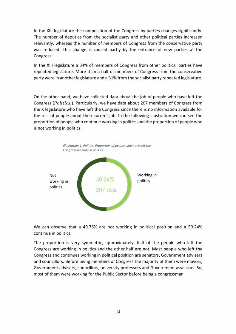
On the other hand, we have collected data about the job of people who have left the

Congress (𝑃𝑜𝑙𝑖𝑡𝑖𝑐𝑠𝑖). Particularly, we have data about 207 members of Congress from

the X legislature who have left the Congress since there is no information available for

the rest of people about their current job. In the following illustration we can see the

proportion of people who continue working in politics and the proportion of people who

is not working in politics.

We can observe that a 49.76% are not working in political position and a 50.24%

continue in politics.

The proportion is very symmetric, approximately, half of the people who left the

Congress are working in politics and the other half are not. Most people who left the

Congress and continues working in political position are senators, Government advisers

and councillors. Before being members of Congress the majority of them were mayors,

Government advisers, councillors, university professors and Government assessors. So,

most of them were working for the Public Sector before being a congressman.

Illustration 1: Politics: Proportion of people who have left the Congress working in politics

50.24%

207 obs.

Working in

politics Not

working in

politics

15

Table 3 displays all provinces and the percentage of lawyers and economists over the

total number of deputies in each province at Congress in each legislature. Highlighted

provinces are those where there are more deputies. In the X legislature Madrid,

Barcelona, Valencia and the Canary Islands had 35, 31, 16 and 15 members of Congress

respectively and in the XII legislature 43, 36, 19 and 17 deputies. Is there any relationship

between the province and the number of lawyers? Are there more lawyers in provinces

with more deputies?

Table 3: Percentage of lawyers and economists by province and legislature

X Legislature XII Legislature

Province % Lawyers % Economists % Lawyers % Economists

Alava 75.0% 0.0% 40.0% 40.0%

Albacete 25.0% 25.0% 40.0% 20.0%

Alicante 33.3% 8.3% 38.5% 30.8%

Almería 33.3% 0.0% 42.9% 0.0%

Asturias 25.0% 0.0% 22.2% 22.2%

Avila 100.0% 0.0% 66.7% 66.7%

Badajoz 33.3% 0.0% 37.5% 12.5% Barcelona 51.6% 3.2% 38.9% 5.6%

Bizkaia 62.5% 12.5% 40.0% 20.0%

Burgos 50.0% 0.0% 50.0% 0.0%

Caceres 25.0% 0.0% 25.0% 0.0%

Cadiz 22.2% 0.0% 54.5% 0.0%

Cantabria 20.0% 20.0% 28.6% 28.6%

Castellón 40.0% 0.0% 33.3% 33.3%

Ceuta 100.0% 0.0% 100.0% 0.0%

Ciudad Real 40.0% 0.0% 40.0% 0.0%

Cordoba 66.7% 16.7% 62.5% 0.0%

Coruña 0.0% 25.0% 37.5% 25.0%

Cuenca 66.7% 0.0% 66.7% 0.0%

Gipuzkoa 50.0% 16.7% 16.7% 0.0%

Girona 50.0% 0.0% 14.3% 0.0%

Granada 42.9% 0.0% 42.9% 0.0%

Guadalajara 66.7% 0.0% 66.7% 0.0%

Huelva 80.0% 0.0% 40.0% 20.0%

Huesca 66.7% 0.0% 0.0% 33.3% Islas Baleares 37.5% 0.0% 37.5% 12.5%

Islas Canarias 20.0% 13.3% 17.6% 11.8%

Jaen 50.0% 16.7% 42.9% 0.0%

La Rioja 25.0% 25.0% 50.0% 25.0%

Leon 100.0% 0.0% 25.0% 0.0%

Lleida 0.0% 0.0% 50.0% 0.0%

Lugo 50.0% 0.0% 25.0% 0.0%

Madrid 22.9% 17.1% 27.9% 23.3%

Malaga 40.0% 20.0% 18.2% 18.2%

Melilla 0.0% 0.0% 100.0% 0.0%

Murcia 30.0% 20.0% 30.8% 15.4%

Navarra 40.0% 20.0% 40.0% 0.0%

Ourense 75.0% 0.0% 75.0% 0.0%

Palencia 66.7% 0.0% 33.3% 33.3%

Pontevedra 0.0% 14.3% 12.5% 25.0%

Salamanca 75.0% 0.0% 75.0% 0.0%

16

Segovia 66.7% 0.0% 66.7% 0.0%

Sevilla 25.0% 16.7% 58.3% 8.3%

Soria 0.0% 50.0% 0.0% 50.0%

Tarragona 33.3% 0.0% 0.0% 16.7%

Teruel 66.7% 33.3% 0.0% 0.0%

Toledo 50.0% 0.0% 42.9% 0.0%

Valencia 43.8% 6.3% 36.8% 5.3%

Valladolid 80.0% 20.0% 33.3% 0.0%

Zamora 66.7% 0.0% 66.7% 0.0%

The percentage of lawyers was reduced in the XII legislature in provinces with more representation at the Congress, that is, the highlighted provinces, but for Madrid where the percentage of lawyers and economists increased from 22.9% to 17.1% and from 17.1% to 23.3% respectively. In the case of Barcelona only the percentage of economists increased approximately by 2.4%.

In order to check if there exist any correlation between the number of deputies in the province and the percentage of lawyers the province, we estimate Model 1 by OLS (Ordinary Least Squares) for both legislatures. Then, we compute the significance tests to see if the number of deputies in the province is relevant to determine the number percentage of lawyers in that province.

%𝐿𝑎𝑤𝑦𝑒𝑟𝑠𝑖 = 𝛼 + 𝛽𝑑𝑒𝑝𝑢𝑡𝑖𝑒𝑠𝑖 (1)

We have tested before if there is any problem of heteroskedasticity in the models by computing the Breusch Pagan Test, in that case we would estimate the models by WLS (Weighted Least Squares), H0: constant variance (homoskedasticity)

HA: heteroskedasticity In both cases we fail to reject the null hypothesis of homoskedasticity since p=0.14>0.05 in the X legislature and p=0.11>0.05 in the XII legislature. Consequently, there is no problem of heteroskedasticity and the OLS estimation is consistent in both cases. There are 52 observations that are the provinces and the autonomic cities of Spain. The null hypothesis and the alternative hypothesis are, 𝐻0: 𝛽 = 0 𝑑𝑒𝑝𝑢𝑡𝑖𝑒𝑠𝑖 is irrelevant and there is no correlation between the number of

deputies in the province and the percentage of lawyers.

𝐻𝐴: 𝛽 ≠ 0 𝑑𝑒𝑝𝑢𝑡𝑖𝑒𝑠𝑖 is relevant and there is a correlation between the number of

deputies in the province and the percentage of lawyers.

17

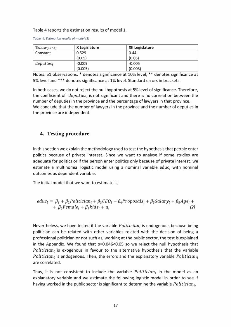
Table 4 reports the estimation results of model 1.

Table 4: Estimation results of model (1)

%𝐿𝑎𝑤𝑦𝑒𝑟𝑠𝑖 X Legislature XII Legislature

Constant 0.529 (0.05)

0.44 (0.05)

𝑑𝑒𝑝𝑢𝑡𝑖𝑒𝑠𝑖 -0.009 (0.005)

-0.005 (0.003)

Notes: 51 observations. * denotes significance at 10% level, ** denotes significance at

5% level and *** denotes significance at 1% level. Standard errors in brackets.

In both cases, we do not reject the null hypothesis at 5% level of significance. Therefore, the coefficient of 𝑑𝑒𝑝𝑢𝑡𝑖𝑒𝑠𝑖 is not significant and there is no correlation between the number of deputies in the province and the percentage of lawyers in that province. We conclude that the number of lawyers in the province and the number of deputies in the province are independent.

4. Testing procedure

In this section we explain the methodology used to test the hypothesis that people enter

politics because of private interest. Since we want to analyse if some studies are

adequate for politics or if the person enter politics only because of private interest, we

estimate a multinomial logistic model using a nominal variable educ𝑖 with nominal

outcomes as dependent variable.

The initial model that we want to estimate is,

𝑒𝑑𝑢𝑐𝑖 = 𝛽1 + 𝛽2𝑃𝑜𝑙𝑖𝑡𝑖𝑐𝑖𝑎𝑛𝑖 + 𝛽3𝐶𝐸𝑂𝑖 + 𝛽4𝑃𝑟𝑜𝑝𝑜𝑠𝑎𝑙𝑠𝑖 + 𝛽5𝑆𝑎𝑙𝑎𝑟𝑦𝑖 + 𝛽5𝐴𝑔𝑒𝑖 +

+ 𝛽6𝐹𝑒𝑚𝑎𝑙𝑒𝑖 + 𝛽7𝑘𝑖𝑑𝑠𝑖 + 𝑢𝑖 (2)

Nevertheless, we have tested if the variable 𝑃𝑜𝑙𝑖𝑡𝑖𝑐𝑖𝑎𝑛𝑖 is endogenous because being

politician can be related with other variables related with the decision of being a

professional politician or not such as, working at the public sector, the test is explained

in the Appendix. We found that p=0.046<0.05 so we reject the null hypothesis that

𝑃𝑜𝑙𝑖𝑡𝑖𝑐𝑖𝑎𝑛𝑖 is exogenous in favour to the alternative hypothesis that the variable

𝑃𝑜𝑙𝑖𝑡𝑖𝑐𝑖𝑎𝑛𝑖 is endogenous. Then, the errors and the explanatory variable 𝑃𝑜𝑙𝑖𝑡𝑖𝑐𝑖𝑎𝑛𝑖

are correlated.

Thus, it is not consistent to include the variable 𝑃𝑜𝑙𝑖𝑡𝑖𝑐𝑖𝑎𝑛𝑖 in the model as an

explanatory variable and we estimate the following logistic model in order to see if

having worked in the public sector is significant to determine the variable 𝑃𝑜𝑙𝑖𝑡𝑖𝑐𝑖𝑎𝑛𝑖.

18

𝑃𝑜𝑙𝑖𝑡𝑖𝑐𝑖𝑎𝑛𝑖 = 𝛽1 + 𝛽2𝑃𝑢𝑏𝑙𝑖𝑐𝑆𝑒𝑐𝑡𝑜𝑟𝑖 + 𝑢𝑖 (3)

The estimation results of the logit model are reported in Table 5.

Table 5: Estimation results of the equation (3)

Politician𝑖 Coefficient Marginal effect, dx/dy

Constant -0.088 (0.172)

PublicSector𝑖 0.829*** (0.192)

0.186*** (0.041)

Notes: 731 observations. * denotes significance at 10% level, ** denotes significance at

5% level and *** denotes significance at 1% level. Standard errors in brackets.

The variable 𝑃𝑢𝑏𝑙𝑖𝑐𝑆𝑒𝑐𝑡𝑜𝑟𝑖 is relevant at 0.1% level of significance, therefore having

worked for the public sector before being member of Congress is significant to

determine if the person is a professional politician or not. If the person has worked for

the public sector the probability of being a professional politician increases, particularly,

in 0.18.

Once we now the variable 𝑃𝑢𝑏𝑙𝑖𝑐𝑆𝑒𝑐𝑡𝑜𝑟𝑖 is relevant to explain the variable 𝑃𝑜𝑙𝑖𝑡𝑖𝑐𝑖𝑎𝑛𝑖,

it is possible to take it as an instrument of the variable 𝑃𝑜𝑙𝑖𝑡𝑖𝑐𝑖𝑎𝑛𝑖 because most people

who have worked in the public sector are professional politicians. Therefore, we

estimate two models, model (4) excluding the variable 𝑃𝑢𝑏𝑙𝑖𝑐𝑆𝑒𝑐𝑡𝑜𝑟𝑖 and model (5)

with the variable 𝑃𝑢𝑏𝑙𝑖𝑐𝑆𝑒𝑐𝑡𝑜𝑟𝑖 so as to compare the results. In addition, we have

checked that there is no correlation between 𝑃𝑢𝑏𝑙𝑖𝑐𝑆𝑒𝑐𝑡𝑜𝑟𝑖 and errors so as not to be

a problem of specification.

The first model is,

𝑒𝑑𝑢𝑐𝑖 = 𝛽1 + 𝛽2𝐶𝐸𝑂𝑖 + 𝛽3𝑃𝑟𝑜𝑝𝑜𝑠𝑎𝑙𝑠𝑖 + 𝛽4𝑆𝑎𝑙𝑎𝑟𝑦𝑖 + 𝛽5𝐴𝑔𝑒𝑖 + 𝛽6𝐹𝑒𝑚𝑎𝑙𝑒𝑖 +

+ 𝛽7𝑘𝑖𝑑𝑠𝑖 + 𝑢𝑖 (4)

The second model is,

𝑒𝑑𝑢𝑐𝑖 = 𝛽1 + 𝛽2𝐶𝐸𝑂𝑖 + 𝛽3𝑃𝑟𝑜𝑝𝑜𝑠𝑎𝑙𝑠𝑖 + 𝛽4𝑆𝑎𝑙𝑎𝑟𝑦𝑖 + 𝛽5𝐴𝑔𝑒𝑖 + 𝛽6𝐹𝑒𝑚𝑎𝑙𝑒𝑖 +

+ 𝛽7𝑘𝑖𝑑𝑠𝑖 + 𝑃𝑢𝑏𝑙𝑖𝑐𝑆𝑒𝑐𝑡𝑜𝑟𝑖 + 𝑢𝑖 (5)

We estimate the multinomial logistic model by Maximum Likelihood method (ML) and

then, we make the following test for both models.

19

In order to test what is the motivation to enter politics we consider the following null

and alternative hypothesis,

𝐻0: 𝛽3 = 𝛽4 = 0 the person enter politics because of private interest

𝐻𝐴: 𝛽3 ≠ 𝑎𝑛𝑑/𝑜𝑟 𝛽4 ≠ 0 the person does not enter politics because of private interest

(public interest)

𝑃𝑟𝑜𝑝𝑜𝑠𝑎𝑙𝑠𝑖: the number of proposals represents the interest in politics of each member

of Congress. If the person is looking for public interest rather than for private interest,

we should obtain a positive and relevant coefficient is since the member would

participate in more initiatives.

𝑆𝑎𝑙𝑎𝑟𝑦𝑖: the salary is related with the number of commissions, the more commissions

the higher salary, therefore, if the person enter politics because of public interest, the

sign of the coefficient should be positive and significant. The salary is not related with

the number of initiatives and the salary is the same for all commissions.

If the person enter politics because of private interest, we should obtain that the

number of proposals and the salary are irrelevant because members in this case are not

really interested in politics so, they are not going to take part in commissions and

proposals.

On the other hand, we consider control variables, the age, the gender and the number

of kids but these variables do not determine whether the person enter politics because

of private interest or not.

Moreover, we cannot interpret the estimated coefficients, only their sign so, we

compute the marginal changes of the variables for each category of the variable educ𝑖

to see what the change in the probabilities is when there is a change in the variable. In

the case of binary variables, the change is discrete from 0 to 1.

5. Results

The following table shows the estimation results from the multinomial logistic models.

The base outcome is outcome 1 (law studies); consequently, all coefficients are

interpreted with respect to a person who has a bachelor’s degree in law. We have 465

observations in the model excluding the variable 𝑃𝑢𝑏𝑙𝑖𝑐𝑆𝑒𝑐𝑡𝑜𝑟𝑖, model 4 and 459

observations in the model including 𝑃𝑢𝑏𝑙𝑖𝑐𝑆𝑒𝑐𝑡𝑜𝑟𝑖, model 5. The reason for not having

743 observations of the X and the XII legislatures, that is, all observations for each

legislature, is that we do not have data for all observations of each explanatory variable.

20

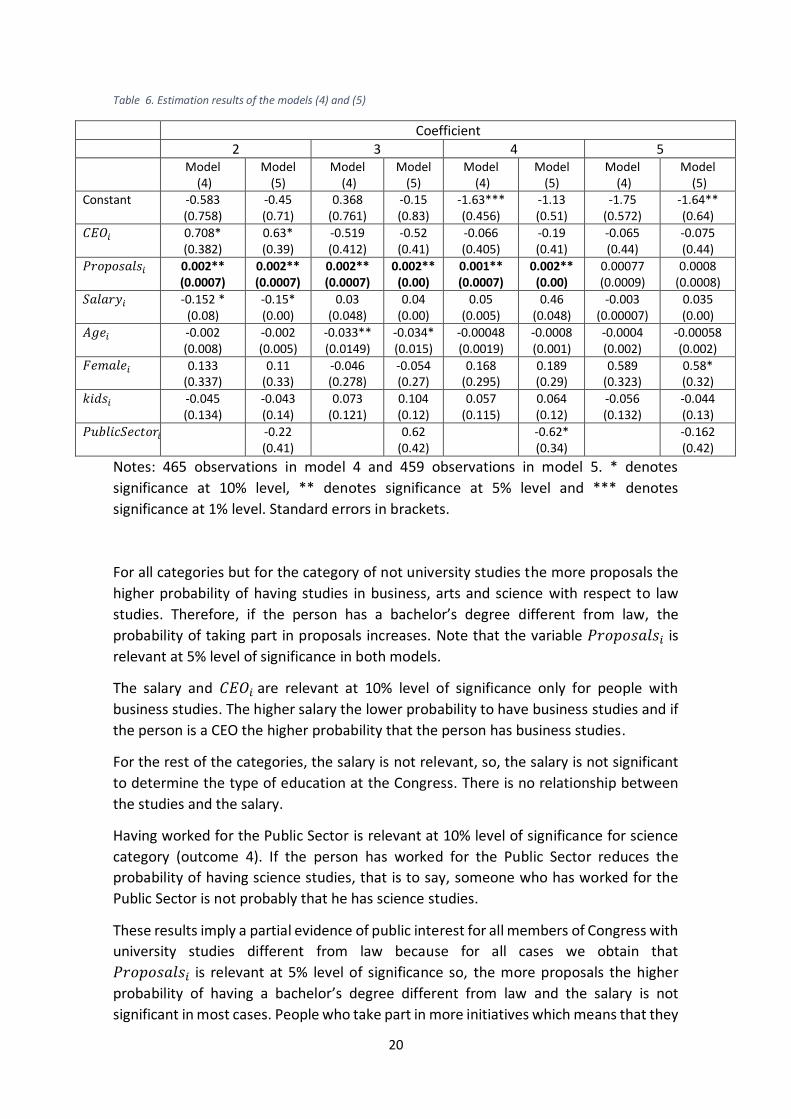
Table 6. Estimation results of the models (4) and (5)

Coefficient

2 3 4 5 Model

(4) Model

(5) Model

(4) Model

(5) Model

(4) Model

(5) Model

(4) Model

(5) Constant -0.583

(0.758) -0.45 (0.71)

0.368 (0.761)

-0.15 (0.83)

-1.63*** (0.456)

-1.13 (0.51)

-1.75 (0.572)

-1.64** (0.64)

𝐶𝐸𝑂𝑖 0.708* (0.382)

0.63* (0.39)

-0.519 (0.412)

-0.52 (0.41)

-0.066 (0.405)

-0.19 (0.41)

-0.065 (0.44)

-0.075 (0.44)

𝑃𝑟𝑜𝑝𝑜𝑠𝑎𝑙𝑠𝑖 0.002** (0.0007)

0.002** (0.0007)

0.002** (0.0007)

0.002** (0.00)

0.001** (0.0007)

0.002** (0.00)

0.00077 (0.0009)

0.0008 (0.0008)

𝑆𝑎𝑙𝑎𝑟𝑦𝑖 -0.152 * (0.08)

-0.15* (0.00)

0.03 (0.048)

0.04 (0.00)

0.05 (0.005)

0.46 (0.048)

-0.003 (0.00007)

0.035 (0.00)

𝐴𝑔𝑒𝑖 -0.002 (0.008)

-0.002 (0.005)

-0.033** (0.0149)

-0.034* (0.015)

-0.00048 (0.0019)

-0.0008 (0.001)

-0.0004 (0.002)

-0.00058 (0.002)

𝐹𝑒𝑚𝑎𝑙𝑒𝑖 0.133 (0.337)

0.11 (0.33)

-0.046 (0.278)

-0.054 (0.27)

0.168 (0.295)

0.189 (0.29)

0.589 (0.323)

0.58* (0.32)

𝑘𝑖𝑑𝑠𝑖 -0.045 (0.134)

-0.043 (0.14)

0.073 (0.121)

0.104 (0.12)

0.057 (0.115)

0.064 (0.12)

-0.056 (0.132)

-0.044 (0.13)

𝑃𝑢𝑏𝑙𝑖𝑐𝑆𝑒𝑐𝑡𝑜𝑟𝑖 -0.22 (0.41)

0.62 (0.42)

-0.62* (0.34)

-0.162 (0.42)

Notes: 465 observations in model 4 and 459 observations in model 5. * denotes

significance at 10% level, ** denotes significance at 5% level and *** denotes

significance at 1% level. Standard errors in brackets.

For all categories but for the category of not university studies the more proposals the

higher probability of having studies in business, arts and science with respect to law

studies. Therefore, if the person has a bachelor’s degree different from law, the

probability of taking part in proposals increases. Note that the variable 𝑃𝑟𝑜𝑝𝑜𝑠𝑎𝑙𝑠𝑖 is

relevant at 5% level of significance in both models.

The salary and 𝐶𝐸𝑂𝑖 are relevant at 10% level of significance only for people with

business studies. The higher salary the lower probability to have business studies and if

the person is a CEO the higher probability that the person has business studies.

For the rest of the categories, the salary is not relevant, so, the salary is not significant

to determine the type of education at the Congress. There is no relationship between

the studies and the salary.

Having worked for the Public Sector is relevant at 10% level of significance for science

category (outcome 4). If the person has worked for the Public Sector reduces the

probability of having science studies, that is to say, someone who has worked for the

Public Sector is not probably that he has science studies.

These results imply a partial evidence of public interest for all members of Congress with

university studies different from law because for all cases we obtain that

𝑃𝑟𝑜𝑝𝑜𝑠𝑎𝑙𝑠𝑖 is relevant at 5% level of significance so, the more proposals the higher

probability of having a bachelor’s degree different from law and the salary is not

significant in most cases. People who take part in more initiatives which means that they

21

are really interested in politics, are more probably to have business studies, arts studies

or science studies.

The estimation results for not university studies category are not very clear, since we do

not obtain significant results.

We also compute marginal changes for each outcome of the variable educ𝑖 in order to

see what the change in the probability of each category is when there is a change in the

explanatory variables. For binary variables the change is a discrete change from 0 to 1,

this is the case of 𝐶𝐸𝑂𝑖, 𝐹𝑒𝑚𝑎𝑙𝑒𝑖 and 𝑃𝑢𝑏𝑙𝑖𝑐𝑆𝑒𝑐𝑡𝑜𝑟𝑖.

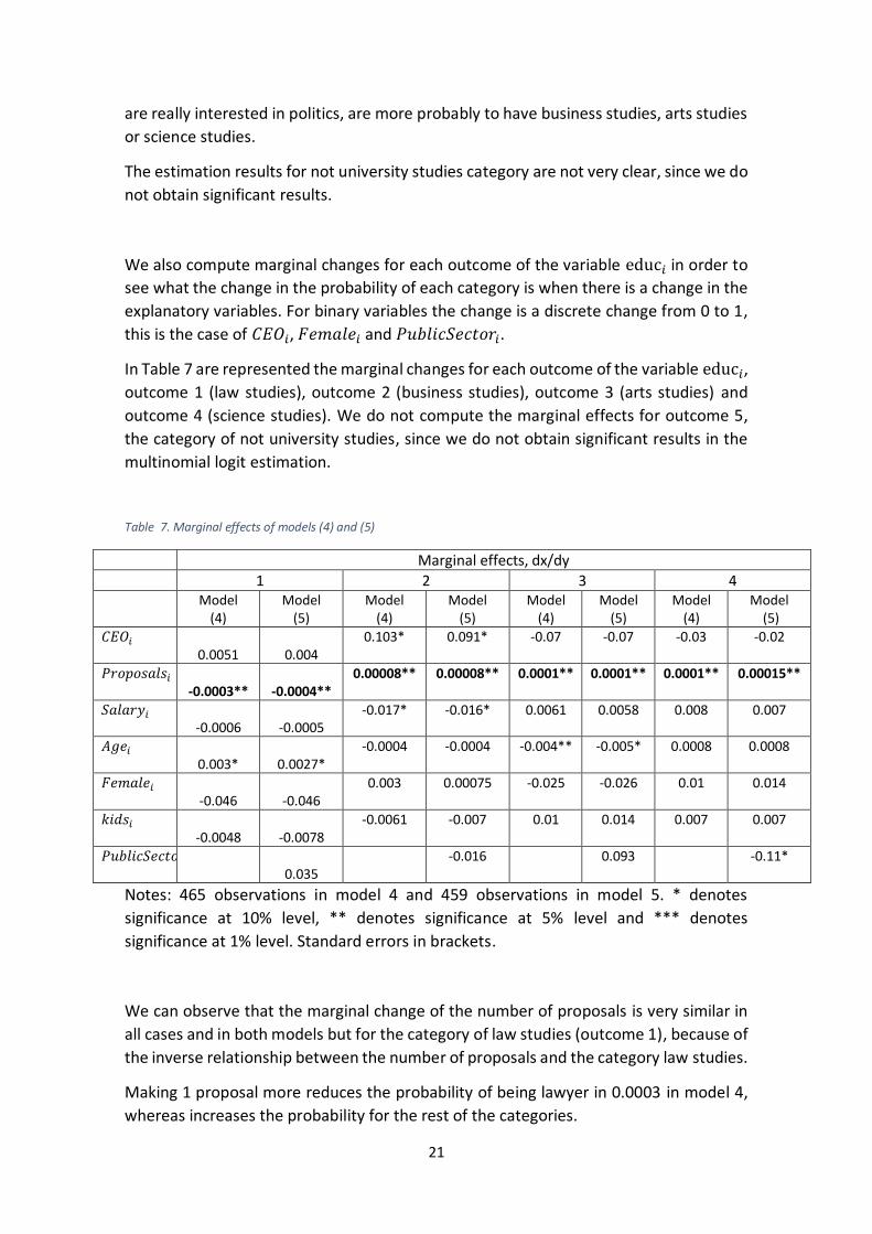
In Table 7 are represented the marginal changes for each outcome of the variable educ𝑖,

outcome 1 (law studies), outcome 2 (business studies), outcome 3 (arts studies) and

outcome 4 (science studies). We do not compute the marginal effects for outcome 5,

the category of not university studies, since we do not obtain significant results in the

multinomial logit estimation.

Table 7. Marginal effects of models (4) and (5)

Marginal effects, dx/dy

1 2 3 4 Model

(4) Model

(5) Model

(4) Model

(5) Model

(4) Model

(5) Model

(4) Model

(5)

𝐶𝐸𝑂𝑖 0.0051 0.004

0.103*

0.091*

-0.07

-0.07

-0.03

-0.02

𝑃𝑟𝑜𝑝𝑜𝑠𝑎𝑙𝑠𝑖 -0.0003** -0.0004**

0.00008**

0.00008**

0.0001**

0.0001**

0.0001**

0.00015**

𝑆𝑎𝑙𝑎𝑟𝑦𝑖 -0.0006 -0.0005

-0.017*

-0.016*

0.0061

0.0058

0.008

0.007

𝐴𝑔𝑒𝑖 0.003* 0.0027*

-0.0004

-0.0004

-0.004**

-0.005*

0.0008

0.0008

𝐹𝑒𝑚𝑎𝑙𝑒𝑖 -0.046 -0.046

0.003

0.00075

-0.025

-0.026

0.01

0.014

𝑘𝑖𝑑𝑠𝑖 -0.0048 -0.0078

-0.0061

-0.007

0.01

0.014

0.007

0.007

𝑃𝑢𝑏𝑙𝑖𝑐𝑆𝑒𝑐𝑡𝑜𝑟𝑖 0.035

-0.016

0.093

-0.11*

Notes: 465 observations in model 4 and 459 observations in model 5. * denotes

significance at 10% level, ** denotes significance at 5% level and *** denotes

significance at 1% level. Standard errors in brackets.

We can observe that the marginal change of the number of proposals is very similar in

all cases and in both models but for the category of law studies (outcome 1), because of

the inverse relationship between the number of proposals and the category law studies.

Making 1 proposal more reduces the probability of being lawyer in 0.0003 in model 4,

whereas increases the probability for the rest of the categories.

22

For science studies, an increase of 1 proposal more increases the probability of a

member of Congress of having a bachelor’s degree in science in 0.0001 in model 4 and

having worked for the Public Sector before decreases the probability in 0.11.

In the case of lawyers there is a partial evidence of private interests, because they tend

to make less proposals.

As we have mentioned, we find that in all categories of university studies but for law

studies there is a partial evidence of public interest since the more proposals the more

probability to have a bachelor’s degree in business, arts or science. Members with

business, arts and science studies are interested in politics because they tend to make

more proposals.

6. Discussion

The aim of this paper was to analyse the motivation of people to enter politics. We have

distinguished between public interest, which represents the real interest in politics and

in maximising social welfare and private interest, which represents the use of politics as

a way to obtain private benefits. This was previously discussed by many authors since

regulation is an important element of politics and it is very related with regulatory failure

and regulatory capture. Several researches about this topic suggested that economic

benefits are not the most important factors of the motivation of people to enter politics.

In order to check what is the motivation to enter politics we have used a database about

Spanish Congressmen of three different legislatures, X legislature, XII legislature and XIII

legislature, which contains personal information about members of Congress and

information about their professional career, to estimate two multinomial logistic models

taking as a dependent variable 𝑒𝑑𝑢𝑐𝑖, which has five categories of education. Like this,

we have been able to observe if the type of education has an influence on the interest

of people to enter politics, if some degrees are more desirable for politics than others

or if there is a private interest behind it. Moreover, we have made a comparison

between legislatures and we have observed that in the most recent legislatures the

distribution of the Congress by parties has changed relevantly.

Along the estimating procedure we have dealt with endogeneity of the variable

Politician𝑖, so we had to collect data about the decision of being a professional politician

such as, if the person had been working in the Public Sector before being a congressman

or not. We found that having worked for the Public Sector before was highly correlated

with being a professional politician. Therefore, we estimated two models, a model

excluding the variable 𝑃𝑢𝑏𝑙𝑖𝑐𝑆𝑒𝑐𝑡𝑜𝑟𝑖 and another model including it to compare the

results. We also, computed the marginal changes of the probabilities to see what the

change in the probabilities is when there is a change in the variable.

23

The estimation results indicated that the education is relevant to see what the

motivation of people is to enter politics. Lawyers are partially motivated by the private

interest since we have obtained that lawyers are less likely to make proposals whereas

the rest of the education categories demonstrated a partial public interest in politics

because they are more likely to make more proposals and take part in more initiatives.

However, the salary is not relevant, so the education and the salary are not correlated.

Making one proposal more decreases the probability of being a lawyer at the Congress

in 0.0003 and increases the probability of having a bachelor’s degree in business in

0.00008, and arts and science in 0.0001.

In conclusion, in this paper we have detected significant differences between

legislatures, and we have made an analysis about Spanish politicians’ motivation. We

have found evidence of the different influence of education on the interest to enter

politics, depending on the type of education the interest in politics can vary. Another

interesting study related with this paper would be to examine the factors that affect the

decision of politicians to stay in politics.

24

7. References

M.R. Borges (2013). Regulation and Regulatory Capture. O. James (1999). Regulation inside government: public interest justifications and regulatory failures. George J. Stigler (1971). The Theory of Economic Regulation. The Bell Journal of Economics and Management Science,Vol. 2,No.1 (Spring, 1971), pp. 3-21. Alcántara Sáez, Manuel. (2017). Political career and political capital. Convergencia, 24(73), 187-204. Available at: http://www.scielo.org.mx/scielo.php?script=sci_arttext&pid=S140514352017000100187&lng=es&tlng=es. Tullock, G. (1967). The welfare costs of tariffs, monopolies and theft. Rice University. Dal Bó, Ernesto (2006). Regulatory capture: a review. Haas School of Business and Travers Department of Political Science, University of California, Berkeley. Gallagher, Michael; Mitchell, Paul. (2005). The Politics of Electoral Systems. Oxford University Press. Keane, Michael; Merlo, Antonio. (2007). Money, Political Ambition and the Career Decisions of Politicians. Timothy, Besley. (2004). Joseph Schumpeter. Paying politicians: Theory and Evidence. LectureJournal of the European Economic Association. Michael E. Levine and Jennifer L. Forrence. (1990). Regulatory Capture, Public Interest, and the Public Agenda: Toward a Synthesis. Journal of Law, Economics, & Organization, Vol. 6, (1990), pp. 167-198. Congreso de los Diputados, Registro de intereses y actividades. Availabe at: http://www.congreso.es. Congreso de los Diputados, Relación conjunta de diputados en activo y de diputados que han causado baja en la legislatura. Available at: http://www.congreso.es.

25

8. Appendix

Testing for endogeneity

In this section it is explained the testing procedure of endogeneity of the

variable Politician𝑖.

If Politician𝑖 is endogenous, 𝐶𝑜𝑣 (Politician𝑖, 𝑢𝑖) ≠ 0.

The initial model is Model 2,

𝑒𝑑𝑢𝑐𝑖 = 𝛽1 + 𝛽2𝑃𝑜𝑙𝑖𝑡𝑖𝑐𝑖𝑎𝑛𝑖 + 𝛽3𝐶𝐸𝑂𝑖 + 𝛽4𝑃𝑟𝑜𝑝𝑜𝑠𝑎𝑙𝑠𝑖 + 𝛽5𝑆𝑎𝑙𝑎𝑟𝑦𝑖 + 𝛽5𝐴𝑔𝑒𝑖

+ 𝛽6𝐹𝑒𝑚𝑎𝑙𝑒𝑖 + 𝛽7𝑘𝑖𝑑𝑠𝑖 + 𝑢𝑖

We take the reduced form for Politician𝑖, and estimate the reduced model taking all

exogenous variables. 𝑃𝑢𝑏𝑙𝑖𝑐𝑆𝑒𝑐𝑡𝑜𝑟𝑖 is an additional variable which does not appear in

the initial model.

Politician𝑖 = 𝛼1 + 𝛼2𝐶𝐸𝑂𝑖 + 𝛼3𝑃𝑟𝑜𝑝𝑜𝑠𝑎𝑙𝑠𝑖 + 𝛼4𝑆𝑎𝑙𝑎𝑟𝑦𝑖 + 𝛼5𝐴𝑔𝑒𝑖 + 𝛼6𝐹𝑒𝑚𝑎𝑙𝑒𝑖

+ 𝛽7𝑘𝑖𝑑𝑠𝑖 + 𝛼8𝑃𝑢𝑏𝑙𝑖𝑐𝑆𝑒𝑐𝑡𝑜𝑟𝑖 + 𝜀𝑖

All explanatory variables of the reduced model are uncorrelated with 𝑢𝑖. Then, now

Politician𝑖 is uncorrelated with 𝑢𝑖 if and only if 𝑢𝑖 and 𝜀𝑖 are uncorrelated. So, what we

want to test is if 𝑢𝑖 and 𝜀𝑖 are uncorrelated.

We introduce 𝜀�̂� in the initial model, Model 2 and we estimate it. Finally, we check if the

variable Politician𝑖 is endogenous or not by the test of endogeneity.

𝑒𝑑𝑢𝑐𝑖 = 𝛽1 + 𝛽2𝑃𝑜𝑙𝑖𝑡𝑖𝑐𝑖𝑎𝑛𝑖 + 𝛽3𝐶𝐸𝑂𝑖 + 𝛽4𝑃𝑟𝑜𝑝𝑜𝑠𝑎𝑙𝑠𝑖 + 𝛽5𝑆𝑎𝑙𝑎𝑟𝑦𝑖 + 𝛽5𝐴𝑔𝑒𝑖

+ 𝛽6𝐹𝑒𝑚𝑎𝑙𝑒𝑖 + 𝛽7𝑘𝑖𝑑𝑠𝑖 + 𝛽8𝜀�̂� + 𝜖𝑖

The hypotheses are,

H0: 𝐸(𝜀𝑖, 𝑢𝑖) = 0 and/or 𝛽8̂ = 0 (𝑃𝑜𝑙𝑖𝑡𝑖𝑐𝑖𝑎𝑛𝑖 is exogenous)

HA: 𝐸(𝜀𝑖 , 𝑢𝑖) ≠ 0 and/or 𝛽8̂ ≠ 0 (𝑃𝑜𝑙𝑖𝑡𝑖𝑐𝑖𝑎𝑛𝑖 is endogenous)

We reject the null hypothesis that 𝑃𝑜𝑙𝑖𝑡𝑖𝑐𝑖𝑎𝑛𝑖 is exogenous in favour to the alternative

hypothesis 𝑃𝑜𝑙𝑖𝑡𝑖𝑐𝑖𝑎𝑛𝑖 is endogenous since the estimated coefficient 𝛽8̂ ≠ 0 and the p-

value of the test is 0.46<0.05. Hence, the variable is endogenous.