public goods game with group competition

1

SENIOR THESIS

CHI ZHANG

Public Goods Game with Group Competition

Abstract

This thesis attempts to propose a possible explanation for non-‐equilibrium

cooperation observed in public goods game experiments by bounded-‐rationality

and a latent realistic background. This paper proposes a public goods game

modeling real situations people face and researches on how rule of thumb plays an

important role in equilibrium selection.

1. Introduction

This attempt of thesis is motivated by the phenomena of non-‐equilibrium

cooperation observed in some Public Goods experiments. The classical Public Goods

2

game, where each player decides his/her own contribution to the Public Goods from

the initial endowment, has a unique equilibrium where each player makes zero

contribution. In various experiments, however, substantial contributions are

observed. Those contributions mostly divide into two categories.

First, substantial contribution in early periods followed by a decline was widely

observed. Some may argue that this in a merely a result of learning the unfamiliar

rules and outcome correspondence. However findings by Andreoni (1988) and Isaac

and Walker (1988) showed that there is a “restart” effect when a second finitely

repeated game takes place, therefore it cannot be explained as such learning

behavior. The second type of non-‐equilibrium contribution is observed in some

experiments with additional mechanisms, such as redistribution proportional to

individual contribution, sanction and communication. In some groups, subjects

maintained a certain level of cooperation, all contributing a positive amount,

through out the entire session.

Although these behaviors could be explained by reciprocity, altruism or social

norms, the formation of such social preferences is not well explained. Purely

claiming these social preferences as a given fact is somewhat unsatisfactory.

Evolutionary explanation of the formation of social norms has been a popular

attempt (Ostrom 2000), however, this thesis is going to take another approach. This

approach is based on bounded rationality and attempts to posit the classical Public

Goods Game in a larger frame. Instead of assuming that people have a fixed type as

in the evolutionary explanation, this thesis claims that subjects, due to bounded

3

rationality, have a rule of thumb, which is optimal in reality. That is the reason for

the existence non-‐equilibrium in the experiments. This thesis is going to construct a

variant of Public Goods game model with group contribution and redistribution, in

an attempt to capture the features in reality that makes cooperation profitable. Then

a computational method called agent-‐based modeling is adopted to simulate the

process of formation of such rule of thumb and how the characteristics would affect

the distribution of equilibrium outcomes.

2. Theoretical Model

2a. Model Specification

Here we introduce a specific type of equilibrium of group competition robust to

randomness.

Definition: An error-‐proof Nash equilibrium is a Nash equilibrium where for any

group, when the contribution of all group members rises or falls by a small amount

simultaneously, the optimal action for each member is to retain the previous

contribution level.

Mathematically, suppose in an equilibrium, the contribution level of all members are

c1, c2, … , cn respectively, then there exists a positive number ε0 , such that for any

member i, any ε<ε0, i’s optimal contribution level facing c-‐i=(c1-‐ε, c2-‐ε, …, ci-‐1-‐ε, ci+1-‐ε,

…, cn-‐ε) or (c1+ε, c2+ε, …, ci-‐1+ε, ci+1+ε, …, cn+ε) is ci.

4

2b. Public Goods game

Definition: A Public Goods game consists of a group of N members. Each member is

endowed with an initial endowment and each independently decides the amount to

contribute to the group account and rest is invested to the member’s private

account. The resources in the group account gain a return of R ∈ (1,N) and the

return is evenly redistributed to each member and the return to the resources in the

private account is 1, solely belonging to the respective subject.

Nash Equilibrium: The MPCR (marginal per capita return) for contribution is R/N,

strictly smaller than 1, which is the MPCR for investment in private account. Thus in

equilibrium, each subject makes zero contribution.

Error-proof equilibrium: as the MPCR’s are constant, the Nash equilibrium is

error-‐proof.

2c. Public Goods Game with efficiency redistribution

One feature popularly studied, not only in game theory, is redistribution (Balafoutas

et al, 2013). In the classic Public Goods Game, the mechanism of redistribution is

just equal division. If part of the return from collective production is redistributed

according to contribution, the MPCR of contribution for each member will increase.

This then is no longer a pure public goods game but still it is of interest here as it

5

captures some characteristics of realistic situations people face, when the

distribution of public goods can be asymmetric, such as education and highways.

Definition: A Public Goods game with efficiency redistribution consists of a group of

N members. Each member is endowed with an initial endowment and each

independently decides the amount to contribute to the group account and rest is

invested to the private account. The resources in the group account gain a return of

R ∈ (1,N) and a proportion α of the return is redistributed according to contribution

and the rest is evenly redistributed to each member and the return to the resources

in the private account is 1, solely belonging to the respective subject.

Nash Equilibrium: The MPCR (marginal per capita return) for contribution is

Rα+R(1 – α)/N. If it’s strictly smaller than 1, which is the MPCR for investment in

private account, then in equilibrium, each subject makes zero contribution. If it’s

strictly larger than 1, then in equilibrium, full contribution is achieved.

Error-proof equilibrium: as the MPCR’s are constant, the Nash equilibrium is

error-‐proof.

2d. Group Competition

In reality, the return of the collective production is not fixed. In fact, the contribution

to the group, in many circumstances, could make a difference in the return, for

example, NBA teams may be competing for the ranking, where the higher ranked

teams generate more income, and the more effort put in, the higher the team is

6

ranked. The classical Public Goods game does not try to model that. The following is

an attempt to capture that incentive.

Definition: A Public Goods game with group competition consists of G groups, each

with N members. Each member, with the same initial endowment, decides

independently the amount of contribution to the respective group account and the

rest is invested on the member’s private account. The groups are ranked in

descending order by their aggregate contribution within each group. Each group

gains a MPCR ri, when the group is ranked ith, where r1>r2>…>rG. Ties are broken by

the tied groups sharing the average MPCR among them. The return from each group

account is evenly redistributed to each member within the respective group.

Nash Equilibrium: The situation where the MPCR from group account is exactly 1

is not of our interest here and thus ignored. Since MPCR is not 1, in equilibrium,

each member is either contributing nothing or everything, and within each group,

members should make the same contribution. Suppose that in equilibrium, there are

S groups achieving full contribution and the rest achieve zero contribution. The

equilibrium induces two inequalities.

First, the MPCR for the contributing members is (r1+r2+…+rS)/(S*N) and it should be

larger than 1.

7

Second, the MPCR from contributing for a deviating member in a non-‐contributing

group is rS+1/N and it should be smaller than 1.

Therefore we have that L≤S≤U, where U=max{l: (r1+r2+…+rl)/l>N} and L=min{u:

ru+1<N}. L and U are the lower and upper bound of the number of groups

cooperating in an equilibrium. Thus for any S, where L≤S≤U, there exists a class of

equilibria where exactly S groups achieve full contribution and the rest of groups

achieve zero contribution.

Error-proof Equilibrium: For any S>L, rs<N, there exists no error-‐proof

equilibrium as if all group members in a contributing group reduce contribution by

a small amount at the same time, then the optimal level of contribution for the

members in this group will become zero.

Thus the only error-‐proof equilibria are the class of equilibria where exactly L

groups achieve full contribution and the rest achieve zero contribution.

2e. Group Competition with efficiency redistribution

The proportion of collective return redistributed according to contribution is an

interesting character to differentiate the groups. Although alpha’s close enough to 1

will allow all groups to benefit from contribution regardless the outcome of the

8

competition, while constrained, assigning different redistribution parameter α’s

creates a spectrum of incentives to contribute among groups.

Definition: A Public Goods game with group competition and efficiency

redistribution consists of G groups, each with N members. The ith group is assigned

a redistribution parameter αj , where α1>α2>…>αG. Each member, with the same

initial endowment, decides independently the amount of contribution to the

respective group account and the rest is invested on the private account. The groups

are ranked in descending order by their aggregate contribution within each group.

Each group gains a MPCR ri, when the group is ranked ith, where r1>r2>…>rG. Ties

are broken by tied groups sharing the average MPCR among them. A proportion αj

of the return is redistributed according to contribution and the rest is evenly

redistributed to each member within the jth group.

Nash Equilibrium: Let f(α)=N/(1-‐α+Nα). From similar inequalities from 2d, we can

get the similar equilibria. For only groups {k1, k2,…, kS} with k1<k2<…<kS, achieve full

contribution and rest achieve zero contribution.

First the MPCR of contribution is (r1+r2+…+rS)*(αk_s+(1-‐αk_s)/N)/S should be larger

than 1.

Second, the MPCR from contributing for a deviating member in a non-‐contributing

group is rS+1*(αk_s+(1-‐αk_s)/N) and it should be smaller than 1.

Therefore the equilibrium requires that

9

(r1+r2+…+rS)/S>max{f(αk_s): s≤S}=f(αk_S), and rS+1≤min{f(αk_s): s>=S+1}=f(αk*),

where k*=min{1,2,…,N}\{k1, k2,…, ks}.

Therefore for each set of groups {k1, k2,…, ks} such that k1<k2<…<ks,

(r1+r2+…+rS)/S>f(αk_s), and rs+1<f(αk*), where k*=min{1,2,…,N}\{k1, k2,…, ks}, there

exists an equilibrium where the groups {k1, k2,…, ks} achieve full contribution and

the rest achieve zero contribution.

Error-proof Equilibrium: For each set of groups {k1, k2,…, ks} such that

k1<k2<…<ks, such that (r1+r2+…+rS)/S>f(αk_s), rs+1<f(αk*), and rs>f(αk_s), there exists

an error-‐proof equilibrium where the groups {k1, k2,…, ks} achieve full contribution

and the rest achieve zero contribution. Such equilibria is obtained by the addition of

the constraint rs>f(αk_s) (noting that f(α) is the minimum MPCR required for a group

with redistribution factor α), which makes the members of the group ks able to

sustain cooperating when all the members deviate by a small amount and thus only

getting rs instead of (r1+r2+…+rS)/S.

This result is still not free of multiplicity as the constraints can still be satisfied by

multiple equilibria.

3. Agent-based Modeling

3a. Overview

The multiplicity we observed from the result in 2e almost makes it meaningless.

While having derived the possible equilibria, yet it’s still not clear what the

10

probabilistic distribution among those from different initial conditions is. In order

to tackle that, in this section, we are going to adopt the method of agent-‐based

modeling, which is a variant of Monte Carlo method. We will adopt autonomous

agents who start from a random initial contribution level and in each period, adjust

their levels of contribution according to their rules of thumb. The initial

contribution level of each agent is randomly assigned and randomness is also

introduced in the adjustment in each period. We repeat this process until the

outcomes converge to an equilibrium (we will guarantee that it happens almost

surely by repeating it for 300 to 500 rounds) and once a game reaches an

equilibrium, then the adjustments will become zero and the situation will be simply

repetitive thereafter. With a large number of such samples (we set the number of

samples to be 50000 here) we can estimate the probabilistic distribution of

equilibria in relation to the characteristics of the rules of thumb. In this section, we

study two features of the rules of thumb: adjustment rate and learning mechanism.

Because in fact, this simulation is essentially how people adapt to fit into the game.

These are actually two of the most important characteristics of such adaption: how

quickly people adapt according to the feedback they get and what they adapt

according to. People may be cautious or bold in adapting. Also people may not be

able to find out the real factors or real marginal rate of return at the beginning. They

then have to make their decisions according to what they can observe, which is the

average return from their investments in the group account. We attempt to capture

the first by adjustment rate, which is the magnitude of adjustment made by an agent

in one period. The second characteristic is of importance as information is a very

11

crucial component of a game and in reality not all information is always available. If

players can’t receive information of how much others have contributed, they might

need a while to learn how the mechanism works and what their marginal returns

are, which might even not happen at all. Therefore it’s reasonable to assume, under

bounded rationality or imperfect information, that agents would consider the

average return (the ratio of amount returned over the amount invested) before they

gain more information and learn about the marginal return. This important trait is

presented by a learning period, during which the average return is assigned a

diminishing weight.

3b. Treatments

We study six treatments in this section – Basic, Adjustment Rate, Learning,

Redistribution, Fixed Learning/Adjustment Rate, and Fixed

Learning/Redistribution. In the Basic Treatment (Treatment B), we follow the basic

group competition setting described in 2d. The agents start out each round with

initial endowment 10. The initial contribution level for each agent is independently

drawn from a uniform random distribution on [0, 10] and the agents adjust their

contribution in by s*h*(MPCR-‐1), where s is the adjustment rate, which is the same

for all agents in this treatment, and h is a random variable distributed uniformly on

[0,1] and MPCR refers to that specific round. As we can see, if MPCR for one agent is

larger than 1, that agent will increase his contribution level in the next round, and if

12

MPCR is smaller than 1, that agent will decrease his contribution level, which seems

intuitive.

In the Adjustment Rate Treatment (Treatment AR), now each group is assigned a

different adjustment rate. In the Learning Treatment, agents consider both their

marginal return and average return from the group accounts. In this treatment,

each group is assigned a learning period Li, and the weight of the marginal return

increases from 1/Li in the first period to 1 in the Li’s period and thereafter. In the

Redistribution Treatment (Treatment R), each group is assigned a redistribution

factor αI, which is the proportion of the return from the group account distributed

according to contribution and the rest is still evenly distributed. In the Fixed

Learning/Adjustment Rate Treatment (Treatment FLAR), all groups have the same

learning period but different adjustment rates. In the Fixed Learning/Redistribution

(Treatment FLR), all groups have the same learning period but different

redistribution factors. The treatments are summarized in the following table:

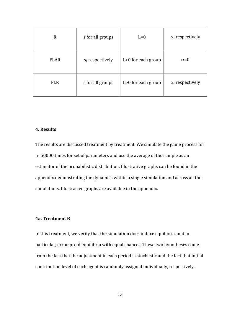
Treatment Adjustment

Rate (s)

Learning Period

(L)

Redistribution

Factor (α)

B s for all groups L=0 α=0

AR si respectively L=0 α=0

L s for all groups Li>0 respectively α=0

13

R s for all groups L=0 αI respectively

FLAR si respectively L>0 for each group α=0

FLR s for all groups L>0 for each group αI respectively

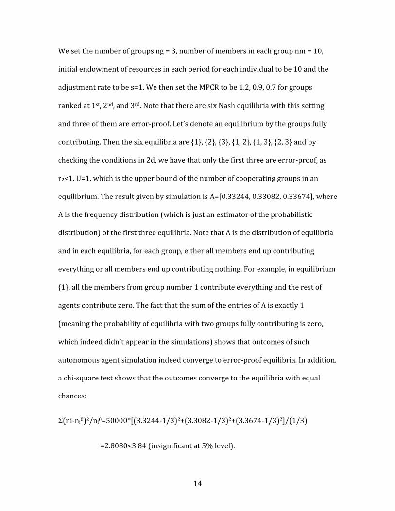
4. Results

The results are discussed treatment by treatment. We simulate the game process for

n=50000 times for set of parameters and use the average of the sample as an

estimator of the probabilistic distribution. Illustrative graphs can be found in the

appendix demonstrating the dynamics within a single simulation and across all the

simulations. Illustrasive graphs are available in the appendix.

4a. Treatment B

In this treatment, we verify that the simulation does induce equilibria, and in

particular, error-‐proof equilibria with equal chances. These two hypotheses come

from the fact that the adjustment in each period is stochastic and the fact that initial

contribution level of each agent is randomly assigned individually, respectively.

14

We set the number of groups ng = 3, number of members in each group nm = 10,

initial endowment of resources in each period for each individual to be 10 and the

adjustment rate to be s=1. We then set the MPCR to be 1.2, 0.9, 0.7 for groups

ranked at 1st, 2nd, and 3rd. Note that there are six Nash equilibria with this setting

and three of them are error-‐proof. Let’s denote an equilibrium by the groups fully

contributing. Then the six equilibria are {1}, {2}, {3}, {1, 2}, {1, 3}, {2, 3} and by

checking the conditions in 2d, we have that only the first three are error-‐proof, as

r2<1, U=1, which is the upper bound of the number of cooperating groups in an

equilibrium. The result given by simulation is A=[0.33244, 0.33082, 0.33674], where

A is the frequency distribution (which is just an estimator of the probabilistic

distribution) of the first three equilibria. Note that A is the distribution of equilibria

and in each equilibria, for each group, either all members end up contributing

everything or all members end up contributing nothing. For example, in equilibrium

{1}, all the members from group number 1 contribute everything and the rest of

agents contribute zero. The fact that the sum of the entries of A is exactly 1

(meaning the probability of equilibria with two groups fully contributing is zero,

which indeed didn’t appear in the simulations) shows that outcomes of such

autonomous agent simulation indeed converge to error-‐proof equilibria. In addition,

a chi-‐square test shows that the outcomes converge to the equilibria with equal

chances:

Σ(ni-‐ni0)2/ni0=50000*[(3.3244-‐1/3)2+(3.3082-‐1/3)2+(3.3674-‐1/3)2]/(1/3)

=2.8080<3.84 (insignificant at 5% level).

15

This treatment serves as a benchmark in comparison to the following treatments.

4b. Treatment AR

In this treatment, the adjustment rate is no longer the same across groups. We set

them to be 2, 1, 0.5 respectively. The other settings are the same. The simulation

gives A=[0.33694, 0.32982, 0.34467], where A is the estimated probabilistic

distribution of equilibria {1}, {2} and {3}.

Our null hypothesis is that the probabilistic distribution is [1/3, 1/3, 1/3]. We use a

multinomial test (chi-‐square test). The chi-‐square statistic is

Σ(ni-‐ni0)2/ni0=50000*[(0.33694-‐1/3)2+(0.329821-‐1/3)2+(0.34467-‐1/3)2]/(1/3)

=517.627>>13.82.

This indicates that the difference is significant at 0.1% level.

To determine whether the relative order of outcomes is related with the order of

adjustment rates or with the level of adjustment rates, we ran another simulation

with s=[3, 1.5, 0.75] and we get A=[0.32900, 0.33482, 0.33618].

Therefore the relative order is indeed related with the level of adjustment however

the functional relation between the adjustment rate and the outcomes is beyond the

scope of this thesis.

16

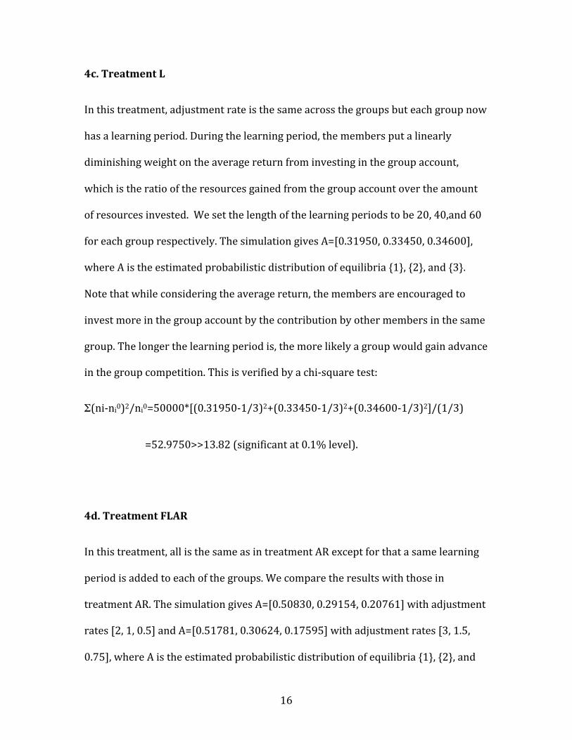
4c. Treatment L

In this treatment, adjustment rate is the same across the groups but each group now

has a learning period. During the learning period, the members put a linearly

diminishing weight on the average return from investing in the group account,

which is the ratio of the resources gained from the group account over the amount

of resources invested. We set the length of the learning periods to be 20, 40,and 60

for each group respectively. The simulation gives A=[0.31950, 0.33450, 0.34600],

where A is the estimated probabilistic distribution of equilibria {1}, {2}, and {3}.

Note that while considering the average return, the members are encouraged to

invest more in the group account by the contribution by other members in the same

group. The longer the learning period is, the more likely a group would gain advance

in the group competition. This is verified by a chi-‐square test:

Σ(ni-‐ni0)2/ni0=50000*[(0.31950-‐1/3)2+(0.33450-‐1/3)2+(0.34600-‐1/3)2]/(1/3)

=52.9750>>13.82 (significant at 0.1% level).

4d. Treatment FLAR

In this treatment, all is the same as in treatment AR except for that a same learning

period is added to each of the groups. We compare the results with those in

treatment AR. The simulation gives A=[0.50830, 0.29154, 0.20761] with adjustment

rates [2, 1, 0.5] and A=[0.51781, 0.30624, 0.17595] with adjustment rates [3, 1.5,

0.75], where A is the estimated probabilistic distribution of equilibria {1}, {2}, and

17

{3}. Comparing these results with the results from treatment AR, we can conclude

that with the learning period, groups with higher adjustment rates are more likely

to thrive in competition. With a learning period, the effect of different adjustment

rates on the distribution of equilibrium outcomes is larger and more oriented.

4e. Treatment R

In this treatment, instead of distributing all the resources in the group account

evenly to each member, part of the resources is distributed to group members

proportional to their individual contribution. We set the redistribution factors (the

proportion of the return from the group account redistributed according to

individual contribution) to be 1/51, 1/171, 0 respectively for the three groups. A

second simulation is run with redistribution factors 1/51, 1/111, 0. We run a third

and a fourth simulation with redistribution factors 1/51, 1/171, 0 and 1/51,

1/111,0 respectively, with adjustment rate s=2. Checking the conditions stated in

2e, we can get the error-‐proof equilibria: {1}, {2}, {3}, {1, 2}, and {1, 3} (checking

one-‐by-‐one all the possible combinations: {1}, {2}, {3}, {1, 2}, {1, 3}, {2, 3}, and {1, 2,

3}). The estimated probabilistic distributions of equilibria {1}, {2}, {3}, {1, 2}, and {1,

3} are as follows (they are estimated by their frequencies in the sample).

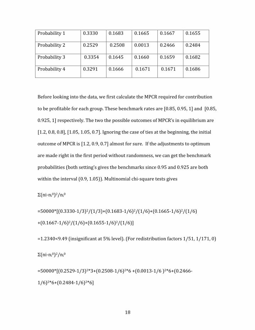
Equilibria (Groups

fully contributing)

1 2 3 1,2 1,3

Benchmark 1/3 1/6 1/6 1/6 1/6

18

Probability 1 0.3330 0.1683 0.1665 0.1667 0.1655

Probability 2 0.2529 0.2508 0.0013 0.2466 0.2484

Probability 3 0.3354 0.1645 0.1660 0.1659 0.1682

Probability 4 0.3291 0.1666 0.1671 0.1671 0.1686

Before looking into the data, we first calculate the MPCR required for contribution

to be profitable for each group. These benchmark rates are [0.85, 0.95, 1] and [0.85,

0.925, 1] respectively. The two the possible outcomes of MPCR’s in equilibrium are

[1.2, 0.8, 0.8], [1.05, 1.05, 0.7]. Ignoring the case of ties at the beginning, the initial

outcome of MPCR is [1.2, 0.9, 0.7] almost for sure. If the adjustments to optimum

are made right in the first period without randomness, we can get the benchmark

probabilities (both setting’s gives the benchmarks since 0.95 and 0.925 are both

within the interval (0.9, 1.05)). Multinomial chi-‐square tests gives

Σ(ni-‐ni0)2/ni0

=50000*[(0.3330-‐1/3)2/(1/3)+(0.1683-‐1/6)2/(1/6)+(0.1665-‐1/6)2/(1/6)

+(0.1667-‐1/6)2/(1/6)+(0.1655-‐1/6)2/(1/6)]

=1.2340<9.49 (insignificant at 5% level). (For redistribution factors 1/51, 1/171, 0)

Σ(ni-‐ni0)2/ni0

=50000*[(0.2529-‐1/3)2*3+(0.2508-‐1/6)2*6 +(0.0013-‐1/6 )2*6+(0.2466-‐

1/6)2*6+(0.2484-‐1/6)2*6]

19

=15229>>18.47(significant at 0.1% level).

Therefore the difference between the simulations with different redistribution

factors is induced by the effect on how the redistribution factors affect the speed of

adjustment each round.

4f. Treatment FLR

This treatment is the same as treatment R except for that all agents adopt a learning

period of the same length 30. We run two simulations with redistribution factors

[1/51, 1/171, 0] and [1/51, 1/111, 0] respectively. The distributions of equilibrium

outcomes are listed as follows.

Equilibria (Groups

fully contributing)

1 2 3 1,2 1,3

Probability 0.3325 0.1657 0.1680 0.1665 0.1672

Probability 0.2633 0.2359 0.0291 0.2384 0.2334

We can observe that the results are quite similar to the results in 4e, which means

that the effect of redistribution does not depend on learning behavior. This is

verified by chi-‐square tests:

Σ(ni-‐ni0)2/ni0

20

=50000*[(0.3330-‐0.3325)2/0.3330+(0.1683-‐0.1657)2/0.1683+(0.1665-‐0.1680

)2/0.1665 +(0.1667-‐0.1665)2/0.1667+(0.1655-‐0.1672)2/0.1655]


Σ(ni-‐ni0)2/ni0

=50000*[(0.2529-‐0.2633)2/0.2529+(0.2508 -‐0.2359)2/0.2508 +(0.0013-‐0.0291

)2/0.0013+(0.2466-‐0.2384)2/0.2466+(0.2484-‐0.2334)2/0.2484]


5. Disccusion

This thesis attempts propose an explantion of cooperation in lab experiments

of Public Goods games by boundned rationality. People enter lab experiments

following their rule of thumb they formed from their everyday life. However

the situation they face in reality may seem similar to lab conditions but may

actually be different. Here we discuss how the role of empirical rule explains

cooperation. Firstly, the Group Competition model proposed by this thesis is

meant to capture some features of realistic situation people face similar to the

public goods game carried out in labs, except for that contribution may actually be

profitable. For example, in a sports leagues, such as NBA, teams are rewarded, in

cash or in reputation, for their rankings in the league. Players gain larger contracts if

their teams play well but the contribution may not be perfectly recognized. Also in

working places, such as offices, when people work on an project together, their

21

individual effort may not be perfectly recognized but the relative competitiveness of

their project determines the cash bonuses they will gain from it. In these situations,

cooperating may indeed be rewarding if enough effort is being made towards prizes

large enough. We can also see that in all the equilibria, all the group members within

a specific group have the same amount of contribution, either full contribution or

zero contribution. This may also explain the fact that people may positively respond

to the cooperation of other players in the sense that from their realistic experiences

that implies they are in a winning group. This model proposes that the seemingly

non-‐equilbrium behaviors may be equilibrium behaviors in a similar game people

face in reality.

Secondly, from the simulation, we can see that bounded rationality and rules of

thumb play an important role in selecting equilibria in the Group Competition

model. The empirical features such as learning (due to bounded rationality or lack of

information) and caution (captured by adjustment rate) are what differentiate the

groups.

Caution can be measured by adjustment rates of agent. Compare the results from

treatment AR and treatment FLAR. With enough information of the marginal return,

a proper level of caution is most beneficial. There is a tradeoff between increasing

contribution quickly to outplay other groups (high adjustment rate) and decreasing

contribution slowly to avoid loss of competitiveness. However, when the

information about marginal return is no longer available from the beginning, a

higher adjustment rate leads to a higher chance of winning.

22

Compare treatment R and treatment FLR. From the chi-‐square tests, the effect of

redistribution factors is not affected by the learning mechanism, thus does not

depend on information. However it depends on adjustment rate as shown in

treatment R.

From treatment L, we can observe that the longer the learning period, the more

advantageous it is to the group. If no information about the marginal return is

available throughout the game, people may even never realize what the marginal

return actually is. This is in fact not rare. In cases such as tax, people have little

information of how much each individual contributes. And in bureaucratic systems,

typically in China, little effort is paid to keep track of the contributions of the

bureaucratic members, neither individual nor aggregage data.

Thirdly, people in reality may also be facing different games. Some may face

situations where more groups are fighting for limited award, which is more

competitive. This might affect the willingness to contribute. Also the efficiency of

redistribution could vary, which accounts for to what extent individual effort is

recognized and rewarded. We can use family as an example as it has a great impact

on individuals. Poor families tend to either hold extremely tight or suffer a total

breakdown, because the competition between groups is severe, and if members see

no chance of getting rewarded, they simply choose to contribute less. Also the

recognition of effort and contribution within a family is a good example of the

redistribution described in this thesis if we consider nonmaterial utilities. People

that grew up in families that respond to individual contributions may tend to be

23

more cooperative as they have been enjoying a higher MPCR. This real life

observation lines up with what we observe in treatment R and FLR, that the higher

the redistribution factor is for a group, the greater are the chances of the group

achieving cooperation

24

Reference

1. Andreoni, J. (1988). Why free ride? : Strategies and learning in public goods

experiments. Journal of Public Economics, 37(3), 291-‐304.

2. Isaac, R. M. & Walker, J. M. (1988). Group Size Effects in Public Good

Provision: The Voluntary Contributions Mechanism. Quarterly Journal of

Economics, 103, 179-199.

3. Ostrom, E. (2000). Collective Action and the Evolution of Social Norms. The

Journal of Economic Perspectives , 14(3), 137-‐158.

4. Smith, E., Gintis, H., & Bowles, S. (2001). Costly Signaling and Cooperation.

Journal of Theoretical Biology, 213, 103-‐119.

5. Balafoutas, L, Kocher, M, Putterman, L & Sutter M. (2013). Equality, Equity

and Incentives: An Experiment. European Economic Review, 60, 32-‐51.

6. Durante, R & Putterman. (2009). Preferences for Redistribution and

Perception of Fairness: An Experimental Study. Working paper

25

Appendix. A Graphs

In this section we show two sets of graphs revealing the dynamic process within

each simulation and across simulations. The graphs are from the simulatio of the

treatments described above, with three groups. In the first subsection, the graphs

are from a typical simulation. The horizontal axis represents the number of rounds

and the vertical axis represents the total contribution of a group. Each group is

represented by a line of different colors. Note that in some graphs we only showed

the first proportion of the whole simulation in order to get a clearer look at the

volatility, which mainly concentrated in the early rounds. In the second subsection,

we demonstrate the convergence of frequency distributions as the results of ever

larger numbers of simulations are averaged together. Each graph in the second

subsection represents a total of 50000 simulations, with the number of simulations

accounted for rising from left to right. The horizontal axis represents the number of

simulations and the vertical represents the frequency of an equilibrium so far. Each

equilibrium, that is, {1} (i.e., the equilibrium in which only members of group 1

cooperate), {2} and {3}, is represented by a line of different colors.

A1. Dynamic Within Simulation

Treatment B

As we can see, only one group prevailed and the other two ended with zero

contribution. In this treatment, the final outcome in largely related to the

initial positions of the group contribution level as groups are identical.

26

Treatment AR

In this treatment, the adjustment rate does make a difference as we expected.

We can see a crossing at the beginning, which is caused by the different rate of

adjustment. We only showed the first 100 rounds to make this crossing clear

enough.

27

Treatment L

In this graph we can see an abrupt change in at the end of a group’s learning

period. This means that the difference between average return and marginal

return is quite significant so that the last weight change in considering

average return make such a difference. We can observe in this graph that

there is tradeoff considering average return. When a group’s total contribtion

level is high, the average return may be much higher than the marginal return

but when the total level is low, the average return may be much lower than the

marginal return, which is the case here in this graph.

28

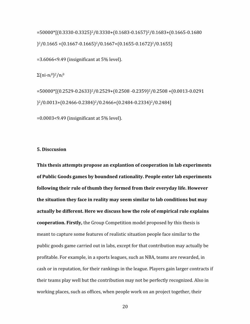
Treatment FLAR

The effect at the end of learning period is similar to the graph right above.

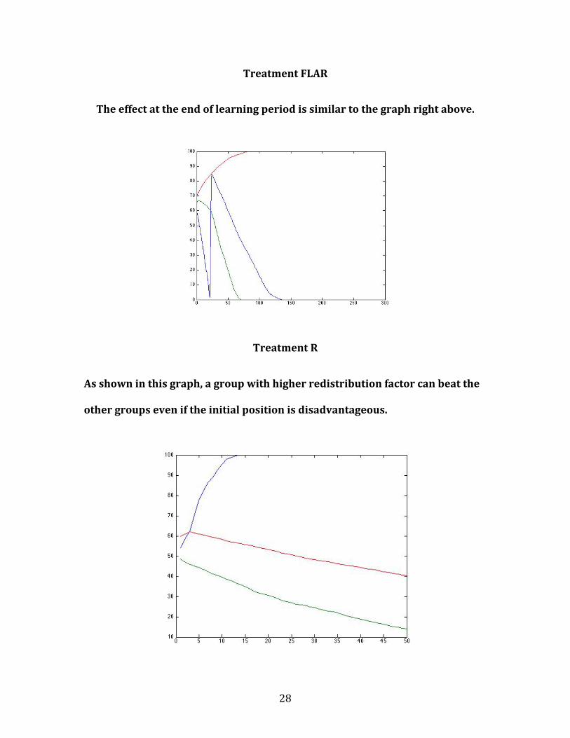
Treatment R

As shown in this graph, a group with higher redistribution factor can beat the

other groups even if the initial position is disadvantageous.

29

Treatment FLR

A2. Convergence across simulations

Treatment B

We can see that the lines approach to be level as the number of simulatiosn

increase.

30

Treatment AR

Treatment L

We only showed the first 500 simulations to illustrate the volatility.

31

Treatment FLAR

32

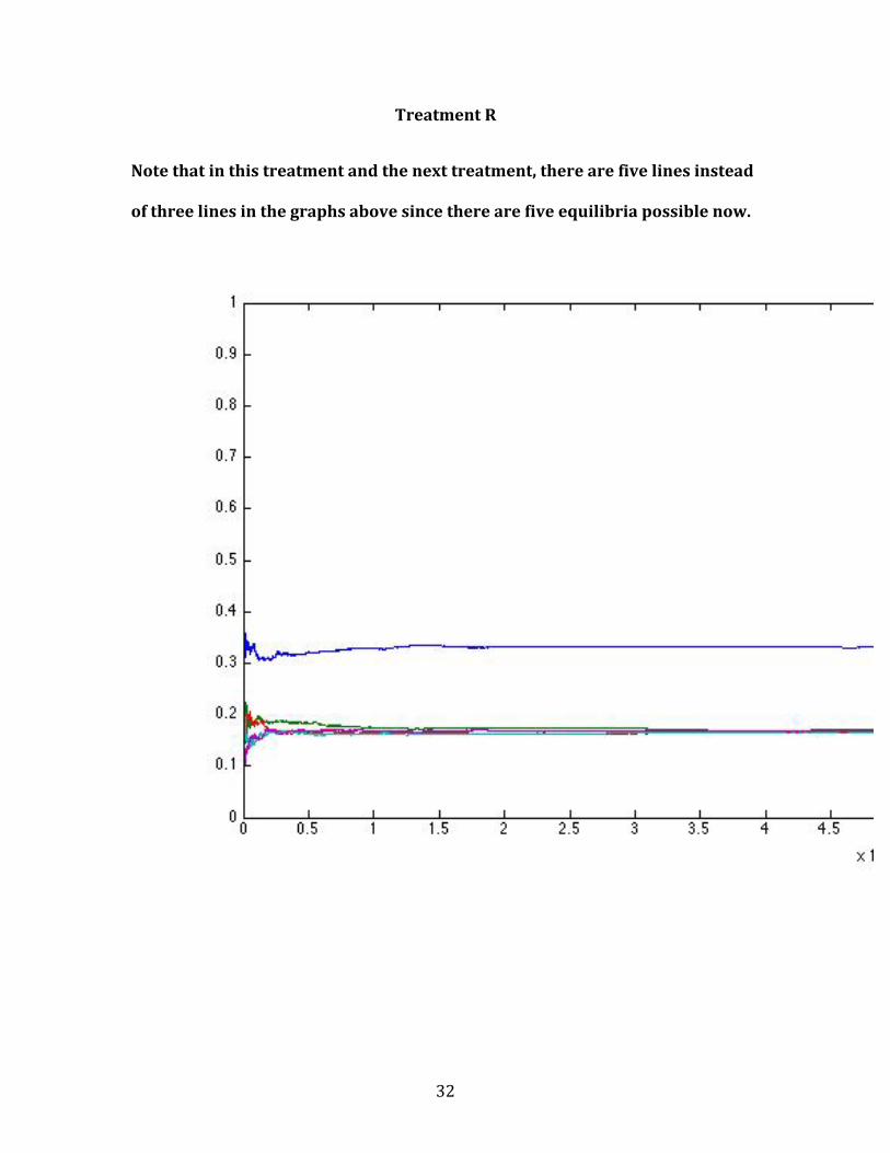
Treatment R

Note that in this treatment and the next treatment, there are five lines instead

of three lines in the graphs above since there are five equilibria possible now.

33

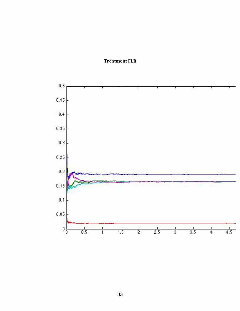
Treatment FLR

34

Appendix. B Simulation Code

1. Treatment B

%Basic_MC r=[1.2,0.9,0.7]; ng=3; nm=10; n=300; s=1; N=50000; A=zeros(3,1); for t=1:N C=10*rand(ng,nm); for i=1:n TC=sum(C,2); R=sortedreturn(TC,r,ng); for g=1:ng for m=1:nm c=rand*s*(R(g)-‐1)+C(g,m); C(g,m)=min(max(c,0),10); end end end A=A+sum(C,2); end A=A/N/nm;

2. Treatment AR

%Agjustment Rate_MC r=[1.2,0.9,0.7]; ng=3; nm=10; n=300; s=[2,1,0.5]; N=50000; A=zeros(3,1); for t=1:N C=10*rand(ng,nm); for i=1:n

35

TC=sum(C,2); R=sortedreturn(TC,r,ng); for g=1:ng for m=1:nm c=rand*s(g)*(R(g)-‐1)+C(g,m); C(g,m)=min(max(c,0),10); end end end A=A+sum(C,2); end A=A/N/nm;

3. Treatment L

%Learning_MC r=[1.2,0.9,0.7]; ng=3; nm=10; n=300; s=1; N=50000; nl=[20,40,60]; A=zeros(3,1); for t=1:N C=10*rand(ng,nm); for i=1:n TC=sum(C,2); R=sortedreturn(TC,r,ng); for g=1:ng for m=1:nm k=nl(g); c=rand*s*((min(i,k)/k+max(k-‐i,0)/k*TC(g)/nm/C(g,m))*R(g)-‐1)+C(g,m); C(g,m)=min(max(c,0),10); end end end A=A+sum(C,2); end A=A/N/nm; 4. Treatment FLAR

36

%Fixed Learning+Adjustment Rate r=[1.2,0.9,0.7]; ng=3; nm=10; n=300; s=[2,1,0.5]; N=50000; nl=30; A=zeros(3,1); for t=1:N C=10*rand(ng,nm); for i=1:n TC=sum(C,2); R=sortedreturn(TC,r,ng); for g=1:ng for m=1:nm c=rand*s(g)*((min(i,nl)/nl+max(nl-‐i,0)/nl*TC(g)/nm/C(g,m))*R(g)-‐1)+C(g,m); C(g,m)=min(max(c,0),10); end end end A=A+sum(C,2); end A=A/N/nm; %Fixed Learning+Adjustment Rate r=[1.2,0.9,0.7]; ng=3; nm=10; n=300; s=[3,1.5,0.75]; N=50000; nl=30; A=zeros(3,1); for t=1:N C=10*rand(ng,nm); for i=1:n TC=sum(C,2); R=sortedreturn(TC,r,ng); for g=1:ng for m=1:nm c=rand*s(g)*((min(i,nl)/nl+max(nl-‐i,0)/nl*TC(g)/nm/C(g,m))*R(g)-‐1)+C(g,m); C(g,m)=min(max(c,0),10); end

37

end end A=A+sum(C,2); end A=A/N/nm; 5. Treatment R %Redistribution_MC r=[1.2,0.9,0.7]; a=[1/51,1/171,0]; ng=3; nm=10; n=500; s=1; N=50000; AA=zeros(3,7); AA(:,1)=[10,0,0]'; AA(:,2)=[0,10,0]'; AA(:,3)=[0,0,10]'; AA(:,4)=[10,10,0]'; AA(:,5)=[10,0,10]'; AA(:,6)=[0,10,10]'; AA(:,7)=[10,10,10]'; A=zeros(3,N); B=zeros(1,7); for t=1:N C=10*rand(ng,nm); for i=1:n TC=sum(C,2); R=sortedreturn(TC,r,ng); for g=1:ng for m=1:nm c=rand*s*((a(g)*nm+1-‐a(g))*R(g)-‐1)+C(g,m); C(g,m)=min(max(c,0),10); end end end TC=sum(C,2); A(:,t)=TC; end A=A/nm; for t=1:N TC=A(:,t); for k=1:7 if sum(AA(:,k)==TC)==3

38

B(k)=B(k)+1; end end end B=B/sum(B); %Redistribution_MC r=[1.2,0.9,0.7]; a=[1/51,1/111,0]; ng=3; nm=10; n=500; s=1; N=50000; AA=zeros(3,7); AA(:,1)=[10,0,0]'; AA(:,2)=[0,10,0]'; AA(:,3)=[0,0,10]'; AA(:,4)=[10,10,0]'; AA(:,5)=[10,0,10]'; AA(:,6)=[0,10,10]'; AA(:,7)=[10,10,10]'; A=zeros(3,N); B=zeros(1,7); for t=1:N C=10*rand(ng,nm); for i=1:n TC=sum(C,2); R=sortedreturn(TC,r,ng); for g=1:ng for m=1:nm c=rand*s*((a(g)*nm+1-‐a(g))*R(g)-‐1)+C(g,m); C(g,m)=min(max(c,0),10); end end end TC=sum(C,2); A(:,t)=TC; end A=A/nm; for t=1:N TC=A(:,t); for k=1:7 if sum(AA(:,k)==TC)==3 B(k)=B(k)+1; end

39

end end B=B/sum(B); 6. Treatment FLR %Fixed Learning+Redistribution_MC r=[1.2,0.9,0.7]; a=[1/51,1/171,0]; ng=3; nm=10; nl=20; n=500; s=1; N=50000; AA=zeros(3,7); AA(:,1)=[10,0,0]'; AA(:,2)=[0,10,0]'; AA(:,3)=[0,0,10]'; AA(:,4)=[10,10,0]'; AA(:,5)=[10,0,10]'; AA(:,6)=[0,10,10]'; AA(:,7)=[10,10,10]'; A=zeros(3,N); B=zeros(1,7); for t=1:N C=10*rand(ng,nm); for i=1:n TC=sum(C,2); R=sortedreturn(TC,r,ng); for g=1:ng for m=1:nm c=rand*s*((min(nl,i)/nl*(a(g)*nm+1-‐a(g))+max(nl-‐i,0)/nl*(TC(g)*(1-‐a(g))/nm/C(g,m)+a(g)))*R(g)-‐1)+C(g,m); C(g,m)=min(max(c,0),10); end end end TC=sum(C,2); A(:,t)=TC; end A=A/nm; for t=1:N TC=A(:,t);

40

for k=1:7 if sum(AA(:,k)==TC)==3 B(k)=B(k)+1; end end end B=B/sum(B); %Fixed Learning+Redistribution_MC r=[1.2,0.9,0.7]; a=[1/51,1/111,0]; ng=3; nm=10; nl=20; n=500; s=1; N=50000; AA=zeros(3,7); AA(:,1)=[10,0,0]'; AA(:,2)=[0,10,0]'; AA(:,3)=[0,0,10]'; AA(:,4)=[10,10,0]'; AA(:,5)=[10,0,10]'; AA(:,6)=[0,10,10]'; AA(:,7)=[10,10,10]'; A=zeros(3,N); B=zeros(1,7); for t=1:N C=10*rand(ng,nm); for i=1:n TC=sum(C,2); R=sortedreturn(TC,r,ng); for g=1:ng for m=1:nm c=rand*s*((min(nl,i)/nl*(a(g)*nm+1-‐a(g))+max(nl-‐i,0)/nl*(TC(g)*(1-‐a(g))/nm/C(g,m)+a(g)))*R(g)-‐1)+C(g,m); C(g,m)=min(max(c,0),10); end end end TC=sum(C,2); A(:,t)=TC; end A=A/nm; for t=1:N TC=A(:,t);

41

for k=1:7 if sum(AA(:,k)==TC)==3 B(k)=B(k)+1; end end end B=B/sum(B);

public goods game with group competition

Documents