public journal of transportation
TRANSCRIPT
Volume 12, No. 4, 2009ISSN 1077-291X
The Journal of Public Transportation is published quarterly by
National Center for Transit ResearchCenter for Urban Transportation Research
University of South Florida • College of Engineering4202 East Fowler Avenue, CUT100
Tampa, Florida 33620-5375Phone: (813) 974-3120
Fax: (813) 974-5168Email: [email protected]
Website: www.nctr.usf.edu/jpt/journal.htm
© 2009 Center for Urban Transportation Research
PublicTransportation
Journal of

iii
Volume 12, No. 4, 2009ISSN 1077-291X
CONTENTS
The Efficiency of Sampling Techniques for NTD ReportingXuehao Chu ...................................................................................................................................................1
Growth Management and Sustainable Transport: Do Growth Management Policies Promote Transit Use?Brian Deal, Jae Hong Kim, Arnab Chakraborty ....................................................................... 21
Bike-sharing: History, Impacts, Models of Provision, and FuturePaul DeMaio .............................................................................................................................................. 41
Service Supply and Customer Satisfaction in Public Transportation: The Quality ParadoxMargareta Friman, Markus Fellesson ............................................................................................ 57
Transit “Pass-Through” Lanes at Freeway Interchanges: A Life-Cycle Evaluation MethodologyMichael Mandelzys, Bruce Hellinga ................................................................................................ 71
A Case Study of Job Access and Reverse Commute Programs in the Chicago, Kansas City, and San Francisco Metropolitan RegionsJ.S. Onésimo Sandoval, Eric Petersen, Kim L. Hunt ................................................................. 93
Design of Transit Signal Priority at Signalized Intersections with Queue Jumper Lanes Guangwei Zhou, Albert Gan ............................................................................................................117
The Efficiency of Sampling Techniques for NTD Reporting
1
The Efficiency of Sampling Techniques for NTD Reporting
Xuehao Chu University of South Florida
Abstract
This paper examines the minimum sample size required by each of six sampling tech-niques for estimating annual passenger miles traveled to meet the Federal Transit Administration’s 95% confidence and 10% precision levels for the National Transit Database. It first describes these sampling techniques in non-technical terms and hypothesizes how they are expected to compare in their minimum sample sizes. It then determines the minimum sample size for 83 actual sample datasets that cover 6 modes and 65 transit agencies. Finally, it summarizes the results in minimum sample size to compare the relative efficiency of these sampling techniques. The potential for improved efficiency from using these sampling techniques is great, but the exact degree of improvement depends highly on individual agencies, modes, and services.
IntroductionTo be eligible for the Urbanized Area Formula Grant Program of the Federal Tran-sit Administration (FTA), transit agencies must report annual passenger miles traveled (PMT) to the Nation Transit Database (NTD) for each combination of mode and type of service (purchased or directly-operated) (FTA 2007, FTA 2008). The NTD requires that a 100% count of annual PMT be reported if it is available and reliable. Getting a 100% account of annual PMT, however, requires keeping track of the distance that every passenger travels. Except in a few cases (e.g., fer-ryboat with only two stops), annual PMT is almost always estimated through
Journal of Public Transportation, Vol. 12, No. 4, 2009
2
statistical sampling, and such an estimate must meet FTA’s 95% confidence and 10% precision levels.
To estimate annual PMT through random sampling, agencies have the burden of developing a sampling plan that meets FTA’s requirements, as well as the sig-nificantly higher burden of collecting the sample data. It is highly desirable to be able to reduce these agency costs while meeting FTA’s confidence and precision requirements.
One strategy to reduce agencies’ burden of developing sampling plans would be to have a user-friendly Excel template for individual agencies to explore and develop sampling plans that are most efficient for their conditions. One example can be found in Chu and Ubaka (2004), but the study was limited to the sampling technique used in FTA’s Circular 2710.1A for motorbus. Chu (2009) develops a more comprehensive template that incorporates a range of sampling techniques that agencies can explore. While the paper uses this new template for analysis, this strategy is not a focus and is not discussed further.
The most effective strategy to reduce agencies’ burden of data collection would be through improving sampling efficiency by taking advantage of modern sampling techniques. Furth (2005), for example, shows the capability of modern sampling techniques to improve sampling efficiency for one agency. This is the focus of this paper.
Many agencies, however, do not consider the relative efficiency of modern sam-pling techniques. The existence of the circular sampling plans for motorbus and demand-response may have discouraged agencies from seeking more efficient sampling plans (UMTA 1988a, UMTA 1988b). More important, agencies may not fully understand the potential cost savings. The literature does not have adequate information on these cost savings. The technical work in the literature typically includes actual examples of cost savings, but these examples are limited to a few cases (Furth 2005) or a few sampling techniques (Furth and McCollom 1987) and are almost always for motorbus only.
The goal of the paper is to encourage agencies to explore the potential of cost savings from using various modern sampling techniques. Toward that goal, the objective is to examine several modern sampling techniques and the potential of reducing agency costs from using them. Specifically, this paper provides the most comprehensive picture of how six modern sampling techniques may perform across a wide range of modes and operating conditions under a uniform process
The Efficiency of Sampling Techniques for NTD Reporting
3
for data analysis. This comprehensive picture helps transit agencies better under-stand the potential cost savings from using these sampling techniques. It also helps transit agencies better understand that the actual efficiency of individual sampling techniques and their relative efficiency depend highly on the mode and the actual operating conditions.
The remainder of the paper first describes six sampling techniques in non-techni-cal terms and hypothesizes how they are expected to compare for their respective minimum sample sizes. It then determines the minimum sample size for 83 actual sample datasets that cover 6 modes and 65 transit agencies. Finally, it summarizes the results in minimum sample size to compare the relative efficiency of these sampling techniques. It also shows the potential and variations in the relative effi-ciency across the sample datasets used.
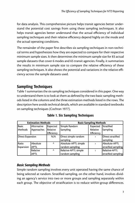
Sampling TechniquesTable 1 summarizes the six sampling techniques considered in this paper. One way to understand them is to look at them as defined by the two basic sampling meth-ods listed in the columns and the three estimation methods listed in the rows. The description here avoids technical details, which are available in standard textbooks on sampling techniques (Cochran 1977).
Table 1. Six Sampling Techniques
Basic Sampling MethodsSimple random sampling involves every unit operated having the same chance of being selected at random. Stratified sampling, on the other hand, involves divid-ing an agency’s service into two or more groups and sampling separately within each group. The objective of stratification is to reduce within-group differences.
Journal of Public Transportation, Vol. 12, No. 4, 2009
4
For an agency that operates both local and express bus services, with the latter having much longer routes, for example, the average passenger trip length (APTL) is likely to vary less across local bus trips or across express bus trips than across all bus trips.
Estimation MethodsThere are two basic methods to estimate PMT—direct expansion and ratio expan-sion. In the case of sampling one-way bus trips, direct expansion involves multiply-ing the average PMT per one-way bus trip in a sample with an expansion factor, or the total number of one-way bus trips actually operated in this case. FTA’s Circular 2710.1A is based on this expansion method for motorbus services (UMTA 1988a). Ratio expansion, on the other hand, involves multiplying the estimate of a ratio from a sample with a known quantity. Estimating PMT as the product of a 100% count of unlinked passenger trips (UPT) and an estimated APTL is one example of ratio expansion. In this case, the APTL is the ratio and the 100% count of UPT is the known quantity. FTA’s Circulars 2710.2A and 2710.4A are based on ratio expansion (UMTA 1988b, UMTA 1988c).
The paper considers two of the three approaches to ratio expansion that have appeared in the literature—one based on absolute APTL, one based on cash rev-enues, and one based on relative APTL. The approach based on absolute APTL is already mentioned above. The approach based on cash revenues uses PMT per dollar of cash-fare revenue as the ratio and total cash-fare revenues as the known quantity. FTA’s Circular 2710.4A is based on the revenue approach (UMTA 1988c) and, because of changing patterns in cash-fare payment over time, FTA no longer approves the sampling plan in this circular without certification by a qualified stat-istician. For the same reason, this paper does not consider the revenue approach any further.
Furth (2005) recently proposed the ratio-expansion approach based on relative APTL. This new approach uses a new known quantity called potential PMT. For any unit of operation along a route (i.e., one one-way vehicle trip, all operations in a year, etc.), its potential PMT is the product of the UPT count on that unit and the route length. In other words, the potential PMT for a given route is its PMT if every passenger traveled the full route length. This new approach uses a relative APTL from a sample as the ratio. For a given route, the relative APTL is the abso-lute APTL over the route length. The relative APTL for a route gives the average fraction of a route’s length that passengers travel on all units of service. A ratio of
The Efficiency of Sampling Techniques for NTD Reporting
5
0.5 for a route, for example, would indicate that, on average, passengers travel one half of the length of the route.
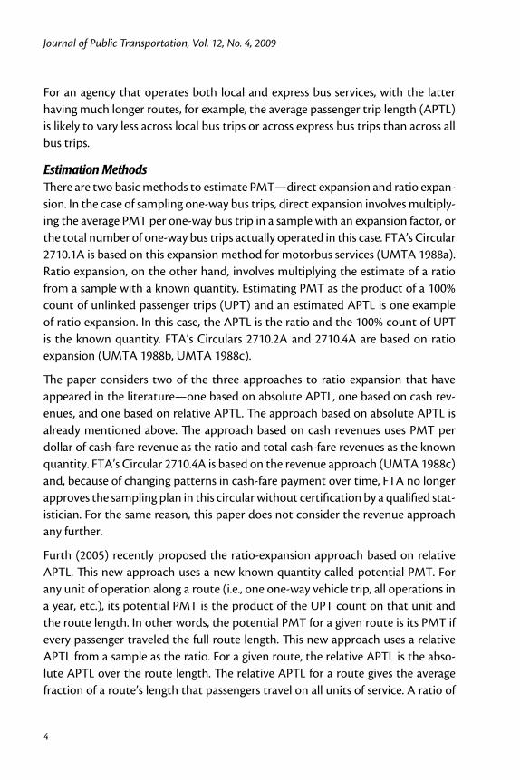
PrerequisitesTable 2 summarizes the prerequisites of these sampling techniques in terms of modes and required data. Direct simple random sampling is applicable to all situ-ations. Each of the other techniques has some prerequisites. These prerequisites are needed for one of three elements of these sampling techniques – stratification, ratio expansion based on absolute APTL, and ratio expansion based on relative APTL. Because the length of a one-way vehicle run can vary for a given route, the average length of each route for the relative-APTL ratio expansion should be cal-culated as the ratio of annual total vehicle revenue miles and annual total vehicle revenue one-way trips along that route.
Table 2. Applicable Modes and Required Data by Sampling Technique
Notes: DR = demand response APTL = average passenger trip length UPT = unlinked passenger trips
Expected Relative EfficiencyTable 1 also summarizes the expected relative efficiency between some of these sampling techniques. Stratification is expected to improve efficiency over simple random sampling for any given estimation method. Otherwise, one would not use stratification because it complicates both data collection and estimation of annual PMT.
Ratio expansion with the absolute-APTL approach is expected to improve effi-ciency over direction expansion with or without stratification. PMT at any unit of operation (e.g., one-way trips) tends to be proportional to the number of UPT
Journal of Public Transportation, Vol. 12, No. 4, 2009
6
for that unit. As a result, it is often more efficient to estimate annual PMT as the product of a 100% count of UPT and the absolute APTL from a sample.
Furth (2005) hypothesizes that the relative-APTL approach is more efficient than the absolute-APTL approach. He argues that PMT at any unit of operation tends to be proportional to not only UPT on the unit but also the route length. Since the product of UPT on a unit of operation and the route length is potential PMT for the unit, PMT on a unit of operation tends to be proportional to potential PMT on that unit. As a result, it is expected to be more efficient to estimate annual PMT by multiplying a 100% count of potential PMT and the relative APTL from a sample by each route in a system.
MethodologyTo analyze the relative efficiency of these six sampling techniques, 83 sample datasets were used that cover 65 agencies and six modes – motorbus, trolleybus, demand-response, vanpool, light rail, and commuter rail with motorbus and trol-leybus combined as a single bus mode for analysis.
AssumptionsAn initial sample size for a given sample dataset to reach the minimum sample size is adjusted for two considerations. One accounts for errors in the sample data. Errors can result from both sampling and non-sampling sources, and these errors may lead to the initial sample size too large or too small for FTA’s requirements. To guard against the latter, a margin of 25% is built into the minimum sample size used in this paper. This margin, however, does not influence the relative efficiency of sampling techniques. The other relates to the minimum size of 10 for each stra-tum when ratio estimation is used. Bias exists in ratio expansion, and it can become significant when the sample size is below 10 (Furth and McCollom 1987).
The results are presented in relative terms. When comparing the efficiency of Absolute-APTL simple random sampling (40) and direct simple random sampling (200), for example, the result is shown as the percent reduction in minimum sam-ple size by Absolute-APTL simple random sampling from direct simple random sampling ((40-200)/200 = -80%).
For ease of references, direct simple random sampling sometimes is referred to as the base technique, while the other five techniques as a whole are referred to as non-base sampling techniques. For motorbus services, using the commonly-used
The Efficiency of Sampling Techniques for NTD Reporting
7
sampling plan in Circular 2710.1A as the base would help transit agencies to deter-mine how much their data collection effort would decline relative to their current effort. Since circular sampling plans are not available for most modes, however, direct simple random sampling is used as the base instead for all modes.
Data Sources and CharacteristicsAmong the 83 sample datasets, 14 are for demand-response, 7 for vanpool, 8 for light rail, 3 for commuter rail, and 51 for bus. According to the Florida Transit Information System, these six modes represent more than 96% of all mode-service type reports submitted to the NTD for 2006. The sample datasets come from two sources. Some are from transit agencies as a result of requests for previous research efforts on sampling for the NTD (Chu and Ubaka 2004, Chu 2006, Chu 2007). Most, however, come from transit agencies in response to a request as part of an effort to develop the National Transit Database Sampling Manual (Chu 2009). This later request was sent to each agency that reported to the NTD for 2006 and was for each mode and type of service that each agency reported. For many agencies that sent their sample datasets for multiple years for a given mode and service type, only the latest is used.
The sampling units vary among the sample datasets both across modes and within a mode. For demand-response and vanpool, the sampling unit is always in vehicle days. For bus, it is in round trips for one sample dataset but in one-way trips for all others. For light rail and commuter rail, the sampling unit is in one-way passenger car trips in most cases but is in one-way train trips for a few of the sample datasets. Not separating the results for different sampling units does not affect the relative efficiency between two sampling techniques.
When applicable, stratification is done differently for different modes and sample datasets with information contained in each sample dataset. There are at least issues with post-stratification:
Information is not always available in a sample dataset for choosing the most •useful way. Stratification depends on the type of quantity on which stratifica-tion is executed and how stratification is done with a chosen quantity.
Stratification is not always based on information available before sampling. •For vanpool, for example, it is done uniformly across all datasets with two strata defined by the sample median of APTL. For bus, stratification is based on route length if available but is based on APTL otherwise. In real applica-
Journal of Public Transportation, Vol. 12, No. 4, 2009
8
tions, one should use something that is known before sampling occurs, such as route length, as the basis for stratification.
As a result, the efficiency of stratification-based sampling techniques may not be exact for each applicable sample dataset. This shortcoming may influence the relative efficiency between stratification and simple random sampling. It does not negatively impact the paper’s main purpose—to motivate transit agencies to explore these sampling techniques.
Actual Relative EfficiencyThis section empirically examines the relative efficiency of the sampling tech-niques from four perspectives. After describing the analysis method, the results for these perspectives are presented in separate sub-sections:
Potentials and Variations shows the potentials in efficiency improvements •from using the various sampling techniques as well as the variations in how each sampling technique may do for a particular case.
Effects of Estimation Methods compares empirically the efficiency of the •different estimation methods for a given basic sampling method. Compari-sons are made separately between Relative-APTL simple random sampling and direct simple random sampling and between the two approaches to ratio expansion.
Effects of Sampling Methods compares empirically the efficiency of the two •basic sampling methods for any given estimation method.
Ratio Expansion versus Stratification examines their relative efficiency •empirically.
Potentials and VariationsThe potential for each sampling technique to improve efficiency is great and can be shown both for individual sample datasets and for all sample datasets com-bined. For individual sample datasets, the potential is evidenced by the highest percent reduction for each applicable sampling technique and mode. The poten-tial is shown between direct simple random sampling and each of the other five sampling techniques.
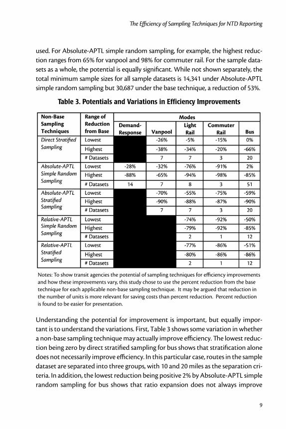
Table 3 shows both minimum and maximum percent reductions in minimum sam-ple size for each non-base sampling technique from the base technique (i.e., direct simple random sampling) by mode. Also shown is the number of sample datasets
The Efficiency of Sampling Techniques for NTD Reporting
9
used. For Absolute-APTL simple random sampling, for example, the highest reduc-tion ranges from 65% for vanpool and 98% for commuter rail. For the sample data-sets as a whole, the potential is equally significant. While not shown separately, the total minimum sample sizes for all sample datasets is 14,341 under Absolute-APTL simple random sampling but 30,687 under the base technique, a reduction of 53%.
Table 3. Potentials and Variations in Efficiency Improvements
Notes: To show transit agencies the potential of sampling techniques for efficiency improvements and how these improvements vary, this study chose to use the percent reduction from the base technique for each applicable non-base sampling technique. It may be argued that reduction in the number of units is more relevant for saving costs than percent reduction. Percent reduction is found to be easier for presentation.
Understanding the potential for improvement is important, but equally impor-tant is to understand the variations. First, Table 3 shows some variation in whether a non-base sampling technique may actually improve efficiency. The lowest reduc-tion being zero by direct stratified sampling for bus shows that stratification alone does not necessarily improve efficiency. In this particular case, routes in the sample dataset are separated into three groups, with 10 and 20 miles as the separation cri-teria. In addition, the lowest reduction being positive 2% by Absolute-APTL simple random sampling for bus shows that ratio expansion does not always improve
Journal of Public Transportation, Vol. 12, No. 4, 2009
10
efficiency over direct expansion. Other than these exceptions, however, these non-base sampling techniques improve efficiency from the base technique. More important, Table 3 shows that the degree of improvements depends highly on the mode and the actual operating conditions through comparing the minimum and maximum reductions for each sampling technique and each mode.
What might be the causes of these large variations in efficiency improvements across the different sample datasets for a given sampling technique? The direct cause of these large variations in efficiency improvements is differences in the degree of varia-tion in the relevant parameter across the different sample datasets. The parameter is PMT per unit of sampling for direct expansion, APTL for Absolute-APTL ratio expansion, and relative passenger trip length for Relative-APTL ratio expansion. For example, the Absolute-APTL approach works well when APTL does not vary much from one vehicle trip to another. This often is the case in transit systems in which the routes have roughly the same length, but not when a transit agency has a mix of long-distance express routes and shorter local routes. If an agency’s routes are of varying length without a clear breakpoint, there is some benefit to stratifying; but if the routes can be neatly divided into very long, express routes and similar-length local routes, stratification can be extremely effective in improving sampling efficiency. In terms of any indirect causes that lead to the differences in the degree of variation in the relevant parameter for a given sampling technique, all we know is that they likely reflect a combination of all service characteristics, including the service geography, the route networks and service polices of all modes in the same service geography, the spatial origin and destination patterns for travelers, etc.
Effects of Estimation MethodsThe effects of estimation methods can be determined in two steps. The first step determines the effects of Absolute-APTL ratio expansion over the base, and the other determines the effects of the Relative-APTL approach over the Absolute-APTL approach. For each step, the analysis is done both without stratification and with stratification.
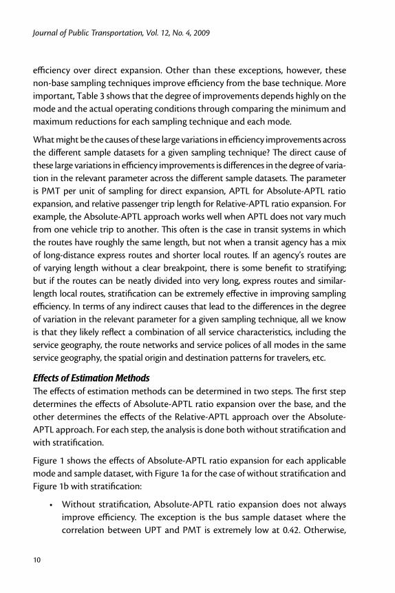
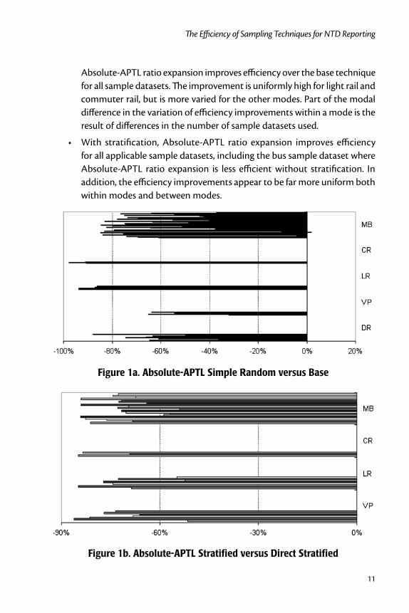
Figure 1 shows the effects of Absolute-APTL ratio expansion for each applicable mode and sample dataset, with Figure 1a for the case of without stratification and Figure 1b with stratification:
Without stratification, Absolute-APTL ratio expansion does not always •improve efficiency. The exception is the bus sample dataset where the correlation between UPT and PMT is extremely low at 0.42. Otherwise,
The Efficiency of Sampling Techniques for NTD Reporting
11
Absolute-APTL ratio expansion improves efficiency over the base technique for all sample datasets. The improvement is uniformly high for light rail and commuter rail, but is more varied for the other modes. Part of the modal difference in the variation of efficiency improvements within a mode is the result of differences in the number of sample datasets used.
With stratification, Absolute-APTL ratio expansion improves efficiency •for all applicable sample datasets, including the bus sample dataset where Absolute-APTL ratio expansion is less efficient without stratification. In addition, the efficiency improvements appear to be far more uniform both within modes and between modes.
Figure 1a. Absolute-APTL Simple Random versus Base
Figure 1b. Absolute-APTL Stratified versus Direct Stratified
Journal of Public Transportation, Vol. 12, No. 4, 2009
12
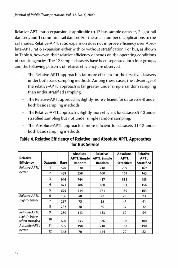
Relative-APTL ratio expansion is applicable to 12 bus sample datasets, 2 light rail datasets, and 1 commuter rail dataset. For the small number of applications to the rail modes, Relative-APTL ratio expansion does not improve efficiency over Abso-lute-APTL ratio expansion either with or without stratification. For bus, as shown in Table 4, however, their relative efficiency depends on the operating conditions of transit agencies. The 12 sample datasets have been separated into four groups, and the following patterns of relative efficiency are observed:
The Relative-APTL approach is far more efficient for the first five datasets •under both basic sampling methods. Among these cases, the advantage of the relative-APTL approach is far greater under simple random sampling than under stratified sampling.
The Relative-APTL approach is slightly more efficient for datasets 6-8 under •both basic sampling methods.
The Relative-APTL approach is slightly more efficient for datasets 9-10 under •stratified sampling but not under simple random sampling.
The Absolute-APTL approach is more efficient for datasets 11-12 under •both basic sampling methods.
Table 4. Relative Efficiency of Relative- and Absolute-APTL Approaches for Bus Service
The Efficiency of Sampling Techniques for NTD Reporting
13
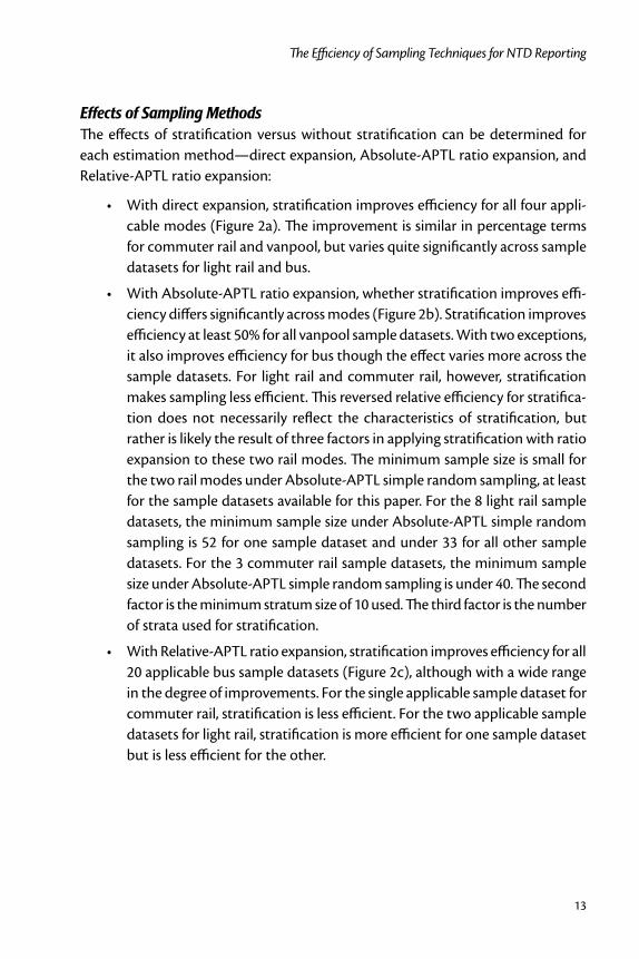
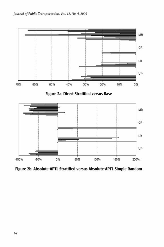
Effects of Sampling MethodsThe effects of stratification versus without stratification can be determined for each estimation method—direct expansion, Absolute-APTL ratio expansion, and Relative-APTL ratio expansion:
With direct expansion, stratification improves efficiency for all four appli-•cable modes (Figure 2a). The improvement is similar in percentage terms for commuter rail and vanpool, but varies quite significantly across sample datasets for light rail and bus.
With Absolute-APTL ratio expansion, whether stratification improves effi-•ciency differs significantly across modes (Figure 2b). Stratification improves efficiency at least 50% for all vanpool sample datasets. With two exceptions, it also improves efficiency for bus though the effect varies more across the sample datasets. For light rail and commuter rail, however, stratification makes sampling less efficient. This reversed relative efficiency for stratifica-tion does not necessarily reflect the characteristics of stratification, but rather is likely the result of three factors in applying stratification with ratio expansion to these two rail modes. The minimum sample size is small for the two rail modes under Absolute-APTL simple random sampling, at least for the sample datasets available for this paper. For the 8 light rail sample datasets, the minimum sample size under Absolute-APTL simple random sampling is 52 for one sample dataset and under 33 for all other sample datasets. For the 3 commuter rail sample datasets, the minimum sample size under Absolute-APTL simple random sampling is under 40. The second factor is the minimum stratum size of 10 used. The third factor is the number of strata used for stratification.
With Relative-APTL ratio expansion, stratification improves efficiency for all •20 applicable bus sample datasets (Figure 2c), although with a wide range in the degree of improvements. For the single applicable sample dataset for commuter rail, stratification is less efficient. For the two applicable sample datasets for light rail, stratification is more efficient for one sample dataset but is less efficient for the other.
Journal of Public Transportation, Vol. 12, No. 4, 2009
14
Figure 2a. Direct Stratified versus Base
Figure 2b. Absolute-APTL Stratified versus Absolute-APTL Simple Random
The Efficiency of Sampling Techniques for NTD Reporting
15
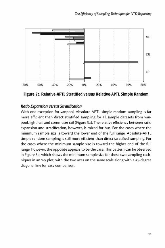
Figure 2c. Relative-APTL Stratified versus Relative-APTL Simple Random
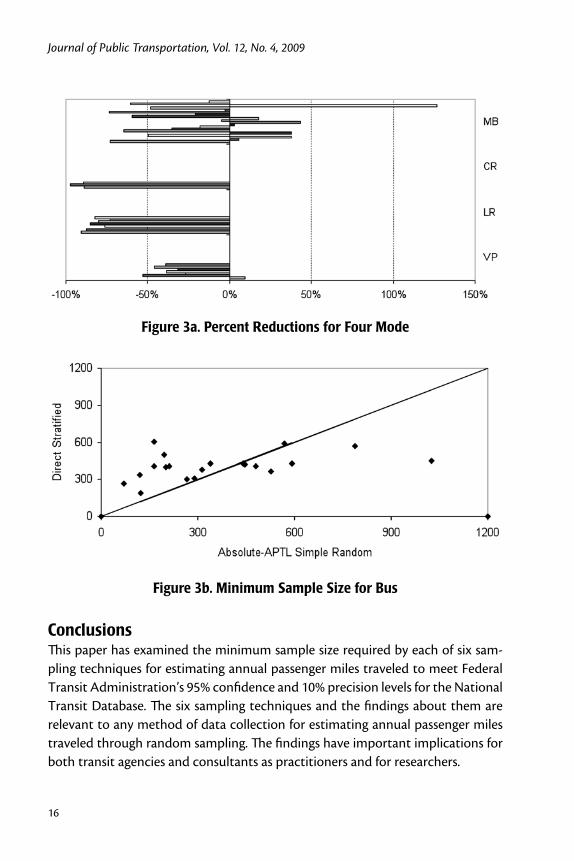
Ratio Expansion versus StratificationWith one exception for vanpool, Absolute-APTL simple random sampling is far more efficient than direct stratified sampling for all sample datasets from van-pool, light rail, and commuter rail (Figure 3a). The relative efficiency between ratio expansion and stratification, however, is mixed for bus. For the cases where the minimum sample size is toward the lower end of the full range, Absolute-APTL simple random sampling is still more efficient than direct stratified sampling. For the cases where the minimum sample size is toward the higher end of the full range, however, the opposite appears to be the case. This pattern can be observed in Figure 3b, which shows the minimum sample size for these two sampling tech-niques in an x-y plot, with the two axes on the same scale along with a 45-degree diagonal line for easy comparison.
Journal of Public Transportation, Vol. 12, No. 4, 2009
16
Figure 3a. Percent Reductions for Four Mode
Figure 3b. Minimum Sample Size for Bus
ConclusionsThis paper has examined the minimum sample size required by each of six sam-pling techniques for estimating annual passenger miles traveled to meet Federal Transit Administration’s 95% confidence and 10% precision levels for the National Transit Database. The six sampling techniques and the findings about them are relevant to any method of data collection for estimating annual passenger miles traveled through random sampling. The findings have important implications for both transit agencies and consultants as practitioners and for researchers.
The Efficiency of Sampling Techniques for NTD Reporting
17
For practitioners, the potential cost savings from using these sampling techniques is great, both for individual cases and for the transit industry as a whole. Practi-tioners should be motivated by these great potentials to consider these sampling techniques. But the actual cost savings for any specific case depends highly on the mode, the operating conditions, and the sampling technique. Practitioners should explore the actual cost savings possible for each sampling technique for their particular mode and operating conditions before deciding whether any of these sampling techniques should be used and which of them should be used.
For researchers, the paper provides the most comprehensive picture of how six modern sampling techniques may perform across a wide range of modes and operating conditions. This comprehensive picture shows that the expected improvement in sampling efficiency for certain sampling techniques can be sig-nificantly greater or significantly less than what researchers have expected from both theoretical considerations and prior limited empirical evidence. For example, estimating passenger miles traveled through ratio expansion on the basis of Relative-APTL has been hypothesized and shown with data from one agency to be more efficient than ratio expansion based on Absolute-APTL (Furth 2005). The results from 12 bus samples, 2 light rail samples, and one commuter rail sample in this paper, however, show that the relative efficiency of these two approaches also vary by mode and the operating conditions of individual cases.
Acknowledgments
The Florida Department of Transportation (FDOT) funded the research through the National Center for Transit Research at the Center for Urban Transportation Research at the University of South Florida. The author would like to thank the many agencies that contributed their sample datasets. The author wants to thank Tara Bartee of FDOT and John Giorgis of FTA for their encouragement and sup-port in developing the National Transit Database Sampling Manual. The author also thanks Peter Furth for his stimulating discussions about the sampling tech-niques and their application to NTD reporting. Comments and suggestions from anonymous reviewers on earlier versions have helped improve the paper.
Journal of Public Transportation, Vol. 12, No. 4, 2009
18
References
Cochran, W. G. 1977. Sampling Techniques, 3rd ed., John Wiley and Sons, Inc., New York.
Chu, X., and I. Ubaka. 2004. A guide to customized sampling plans for National Transit Database reporting. Journal of Public Transportation 7: 21-47.
Chu, X. 2006. Ridership accuracy and transit formula grants. Transportation Research Record 1986: 3-10.
Chu, X. 2007. Another look at FTA approved sampling plans for fixed-route bus services. Transportation Research Record 1992: 113-120.
Chu, X. 2009. Development of Comprehensive Guidance on Obtaining Service Consumed Data for NTD. Center for Urban Transportation Research, Tampa, Florida.
Federal Transit Administration. 2007. Fiscal year 2007 apportionments and alloca-tions and program information. Federal Register 72: 13872-13966.
Federal Transit Administration. 2008. 2008 Annual National Transit Database Reporting Manual. At http://www.ntdprogram.gov/ntdprogram/annual.htm, accessed on July 23, 2008. FDOT (2008), Florida Transit Information System, at http://www.ftis.org/, accessed on July 23, 2008.
Furth, P. G., and B. McCollom. 1987. Using conversion factors to lower transit data collection costs. Transportation Research Record 1144: 1-6.
Furth, P. G. 2005. Sampling and estimation techniques for estimating bus system passenger miles. Journal of Transportation and Statistics 8: 87-100.
Urban Mass Transportation Administration (UMTA). 1988a. Sampling Procedures for Obtaining Fixed Route Bus Operating Data Under the Section 15 Reporting System, Circular UMTA-C-2710.1A, U.S. Department of Transportation.
Urban Mass Transportation Administration (UMTA). 1988b. Sampling Procedures for Obtaining Demand-Responsive Bus System Operating Data Required Under the Section 15 Reporting System, Circular UMTA-C-2710.2A, U.S. Department of Transportation.
Urban Mass Transportation Administration (UMTA). 1988c. Revenue Based Sam-pling Procedures for Obtaining Fixed Route Bus Operating Data Required Under
The Efficiency of Sampling Techniques for NTD Reporting
19
the Section 15 Reporting System, Circular UMTA-C-2810.4A, U.S. Department of Transportation.
About the Author
Dr. Chu ([email protected]) is a Senior Research Associate at the Center for Urban Transportation Research at the University of South Florida in Tampa. He has a Ph.D. in economics from the University of California at Irvine. He has published widely in economics and transportation journals, including the Journal of Transport Eco-nomics and Policy, Transportation, and Transportation Research and is a referee of articles for many international journals, including the Journal of Political Economy and Transportation Science. He served on the Editorial Board of Transportation Research-Part A during 2001–2003 and currently is on the Editorial Board of the Journal of Transportation Safety and Security. He has conducted extensive research on the accuracy of service-consumed data reported to the NTD and on sampling techniques, including both FTA Circular 2710.1A sampling plans and alternative sampling techniques. He has served as a qualified statistician to certify or to develop and certify alternative sampling techniques for many transit agencies for both fixed-route and vanpool services and recently proposed to the FTA the National Transit Database Sampling Manual that includes comprehensive guidance for individual transit agencies to obtain data on passenger miles traveled and unlinked passenger trips for all modes and services.

Journal of Public Transportation, Vol. 12, No. 4, 2009
20
21
Growth Management and Sustainable Transport
Growth Management and Sustainable Transport:
Do Growth Management Policies Promote Transit Use?
Brian Deal, Jae Hong Kim, Arnab Chakraborty University of Illinois
Abstract
Advocates of sustainable development typically consider mass transit to be more sustainable than their automobile-dependent alternatives and desire policies that can achieve higher use of urban mass transit. In this paper, we hypothesize that state-level growth management policies should increase transit use in two ways: first, by limiting core abandonment while accommodating potential increases in population, reducing development elsewhere; and second, by directing new development where transit systems are already well established. We tested this by analyzing 95 metro-politan areas across the United States, 16 with growth-management policies and 79 without. We found that the first set showed a statistically significant improvement in the percentage transit users. The empirical analysis on causality, however, suggests that the improvement is more likely due to an increase in occupancy rates within core areas, by limiting abandonment, rather than in shifting the location of new develop-ment to transit areas.
Journal of Public Transportation, Vol. 12, No. 4, 2009
22
IntroductionThe realization that our current ways of living are implicating our quality of life and even our personal human rights have lead to an understanding of the need for alternatives to our current urban development approaches (Daly 1996, Hawken et al.1999). In the realm of urban policy and planning literature, these alternative development modes go by names such as sustainable development, smart growth, new urbanism, and low-impact development. Although somewhat disparate in their approaches, they all advocate a continual improvement in the quality of life of our communities. To date, they generally have focused more on questions of land use than on transport. Some have suggested, however, that a higher priority needs to be placed on sustainable urban transportation systems, because urban transport systems represent the largest and greatest environmental and social opportunity to improving community quality of life (May et al. 2003, Holden et al. 2005)
Progress toward more sustainable transport faces many barriers and challenges (Black 2000, TRB 1997, Hull 2008). According to decennial census data and the American Community Survey of 2005, auto-based travel remains the norm, while the percentages of commuters using transit, biking, and walking have declined steadily from 1990 to 2005. Assuming a continued increase in travel demand and a lack of infrastructure improvements in transit and other alternatives modes, these trends are likely to continue without policy interventions.
Many different approaches and policies to counteract unsustainable transport trends have been proposed in the recent literature (TRB 1997, Hull 2008, Rich-ardson 1999, Richardson 2005, Deakin 2002, May et al. 2007, Banister 2008). The approach to sustainable transport depends on the definition of the concept. Although the definition of the term sustainability may differ depending on the context, there are certain social, economic, and environmental factors shared among different transport sustainability concepts (May et al. 2007, Jabareen 2006, Litman et al. 2006). From these perspectives, transit is viewed favorably and con-sidered more sustainable than automobiles (Litman 2007), even though modern automobiles pollute much less than their predecessors and transit vehicles often run while relatively empty. The central question for advocates of sustainable trans-port is how to encourage the use of mass transit. This paper examines the effects of macro-level land use planning policies on transit mode choice and use (Figure 1). We analyze a specific policy approach—growth management—and examine its potential efficacy by measuring its impact on commuter transit use.

23
Growth Management and Sustainable Transport
Sour
ces:
(TRB
199
7, H
ull 2
008,
Ric
hard
son
1999
, Ric
hard
son
2005
, Dea
kin
2002
, May
et a
l.200
7, B
anist
er 2
008)
; Eac
h in
ters
ectio
n re
pre-
sent
s a w
ay o
f ach
ievi
ng su
stai
nabl
e tr
ansp
ort—
e.g., w
e ca
n en
cour
age
sust
aina
ble
mod
e ch
oice
s by
usin
g ta
x, p
ricin
g, or
oth
er fi
nanc
ial
polic
y in
stru
men
ts.
Figu
re 1
. Mat
rix
Show
ing
Sust
aina
ble
Dev
elop
men
t App
roac
hes
Des
crib
ed in
the
Lite
ratu
re
Journal of Public Transportation, Vol. 12, No. 4, 2009
24
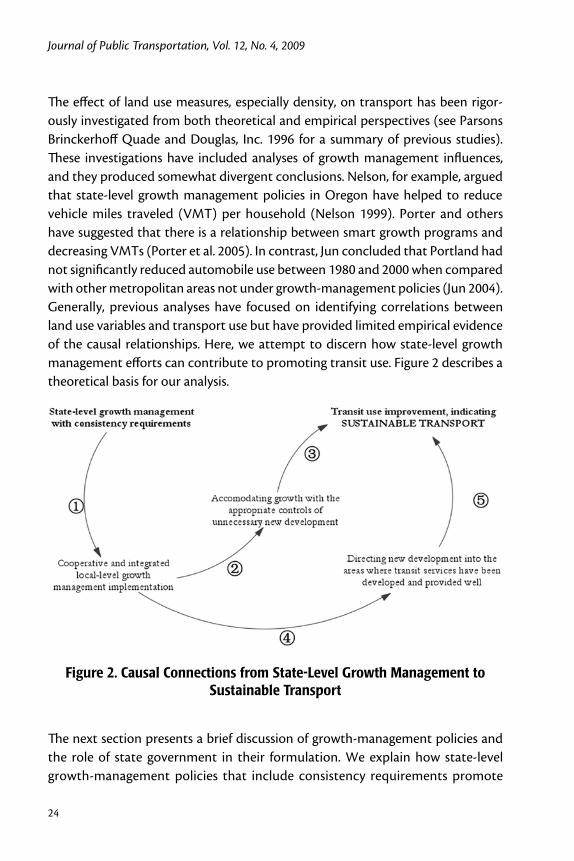
The effect of land use measures, especially density, on transport has been rigor-ously investigated from both theoretical and empirical perspectives (see Parsons Brinckerhoff Quade and Douglas, Inc. 1996 for a summary of previous studies). These investigations have included analyses of growth management influences, and they produced somewhat divergent conclusions. Nelson, for example, argued that state-level growth management policies in Oregon have helped to reduce vehicle miles traveled (VMT) per household (Nelson 1999). Porter and others have suggested that there is a relationship between smart growth programs and decreasing VMTs (Porter et al. 2005). In contrast, Jun concluded that Portland had not significantly reduced automobile use between 1980 and 2000 when compared with other metropolitan areas not under growth-management policies (Jun 2004). Generally, previous analyses have focused on identifying correlations between land use variables and transport use but have provided limited empirical evidence of the causal relationships. Here, we attempt to discern how state-level growth management efforts can contribute to promoting transit use. Figure 2 describes a theoretical basis for our analysis.
Figure 2. Causal Connections from State-Level Growth Management to Sustainable Transport
The next section presents a brief discussion of growth-management policies and the role of state government in their formulation. We explain how state-level growth-management policies that include consistency requirements promote
25
Growth Management and Sustainable Transport
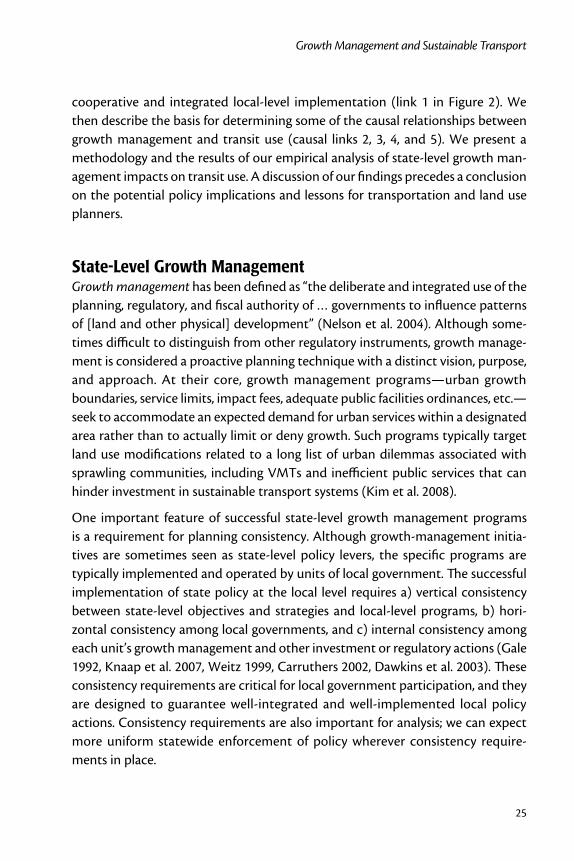
cooperative and integrated local-level implementation (link 1 in Figure 2). We then describe the basis for determining some of the causal relationships between growth management and transit use (causal links 2, 3, 4, and 5). We present a methodology and the results of our empirical analysis of state-level growth man-agement impacts on transit use. A discussion of our findings precedes a conclusion on the potential policy implications and lessons for transportation and land use planners.
State-Level Growth ManagementGrowth management has been defined as “the deliberate and integrated use of the planning, regulatory, and fiscal authority of … governments to influence patterns of [land and other physical] development” (Nelson et al. 2004). Although some-times difficult to distinguish from other regulatory instruments, growth manage-ment is considered a proactive planning technique with a distinct vision, purpose, and approach. At their core, growth management programs—urban growth boundaries, service limits, impact fees, adequate public facilities ordinances, etc.—seek to accommodate an expected demand for urban services within a designated area rather than to actually limit or deny growth. Such programs typically target land use modifications related to a long list of urban dilemmas associated with sprawling communities, including VMTs and inefficient public services that can hinder investment in sustainable transport systems (Kim et al. 2008).
One important feature of successful state-level growth management programs is a requirement for planning consistency. Although growth-management initia-tives are sometimes seen as state-level policy levers, the specific programs are typically implemented and operated by units of local government. The successful implementation of state policy at the local level requires a) vertical consistency between state-level objectives and strategies and local-level programs, b) hori-zontal consistency among local governments, and c) internal consistency among each unit’s growth management and other investment or regulatory actions (Gale 1992, Knaap et al. 2007, Weitz 1999, Carruthers 2002, Dawkins et al. 2003). These consistency requirements are critical for local government participation, and they are designed to guarantee well-integrated and well-implemented local policy actions. Consistency requirements are also important for analysis; we can expect more uniform statewide enforcement of policy wherever consistency require-ments in place.

Journal of Public Transportation, Vol. 12, No. 4, 2009
26
The presence of state-level growth-management policies that include consistency requirements are typically used to distinguish growth-management areas from non-growth management areas (see, for example, Carruthers 2002 and Dawkins et al. 2003), although there is disagreement on which states this encompasses (Weitz 1999, Dawkins et al. 2003). Dawkins and Nelson have identified eight states they believe meet the criteria—Florida, Maine, Maryland, New Jersey, Oregon, Rhode Island, Vermont, and Washington (Dawkins et al. 2003). Porter includes Georgia (Porter 1996), and Anthony expands the list to include California and Hawaii (Anthony 2004). In this work, we used the eight states identified by Dawkins and Nelson (Dawkins et al. 2003), mainly because consistency requirements were included directly in the identification process. Table 1 lists the eight growth-management states used in this study.
Table 1. Eight U.S. States Having Proactive Growth Management (Effective Prior to 2000)
StateConsistency
Requirements a Type b
Rank by Sierra Club c
Florida V, H, I State Dominant 11th
Maine V, H, I State Dominant 7th
Maryland V, I - 3rd
New Jersey I State-Local Negotiated
17th
Oregon V, I State Dominant 1st
Rhode Island V, H, I State Dominant 10th
Vermont H, I Regional-Local Cooperative
2nd
Washington H, I Fusion 5th
Sources: Gale 1992, Dawkins et al. 2003, Sierra Club 1999 a V, H, and I refer to vertical consistency, horizontal consistency, and
internal consistency, respectively.b Gale classified state-sponsored growth management into four
categories – a) state-dominant, b) regional-local cooperative, c) state-local negotiated, and d) fusion (Gale 1992).
c Sierra Club evaluated 50 U.S. states in terms of land use planning efforts to control sprawl (Sierra Club 1999
27
Growth Management and Sustainable Transport
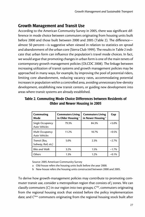
Growth Management and Transit UseAccording to the American Community Survey in 2005, there was significant dif-ference in mode choice between commuters originating from housing units built before 2000 and those built between 2000 and 2005 (Table 2). The difference—almost 50 percent—is suggestive when viewed in relation to statistics on sprawl and abandonment of the urban core (Sierra Club 1999). The results in Table 2 indi-cate that urban form can influence the population’s travel mode choices. In fact, we would argue that promoting changes in urban form is one of the main tenets of contemporary growth management policies (OLCDC 2008). The linkage between increasing utilization of transit systems and growth management policies may be approached in many ways, for example, by improving the pool of potential riders, limiting core abandonment, reducing vacancy rates, accommodating potential increases in population within a controlled area, avoiding unnecessary low-density development, establishing new transit centers, or guiding new development into areas where transit systems are already established.
Table 2. Commuting Mode Choice Differences between Residents of Older and Newer Housing in 2005
Commuting Mode
Commuters Living in Older Housing a
Commuters Living in Newer Housing b
Gap
Single Occupancy Auto Vehicles
79.3% 84.3% +5.0%
Multi Occupancy Auto Vehicles
11.2% 10.7% –0.5%
Transit (Bus, Subway, Rail, etc)
5.0% 2.3% –2.7%
Bike and Walk 3.2% 1.5% –1.7%
Others 1.3% 1.2% –0.1%
Source: 2005 American Community Surveya Old-house refers the housing units built before the year 2000. b New-house refers the housing units constructed between 2000 and 2005.
To derive how growth-management policies may contribute to promoting com-muter transit use, consider a metropolitan region that consists of j zones. We can classify commuters (C) in our region into two groups; COld, commuters originating from the regional housing stock that existed before the policy implementation date; and CNew commuters originating from the regional housing stock built after
Journal of Public Transportation, Vol. 12, No. 4, 2009
28
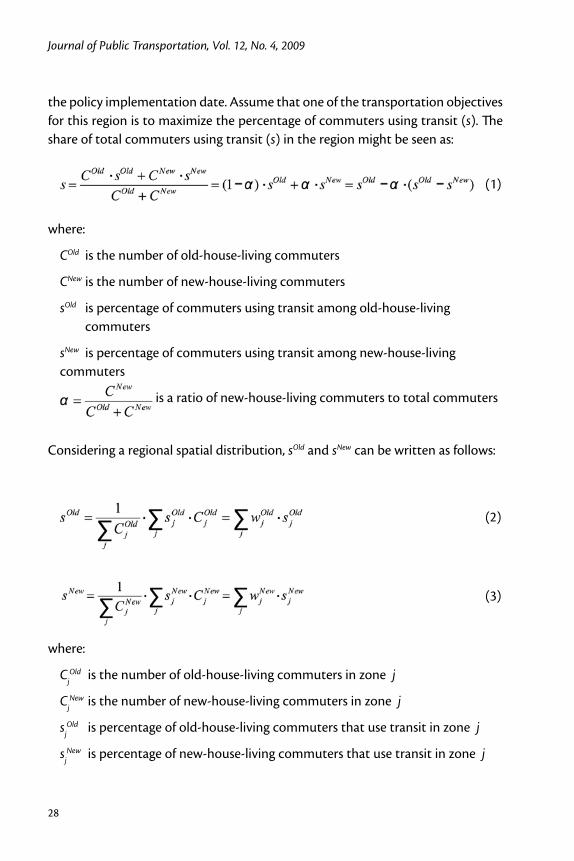
the policy implementation date. Assume that one of the transportation objectives for this region is to maximize the percentage of commuters using transit (s). The share of total commuters using transit (s) in the region might be seen as:
(1)
where:
COld is the number of old-house-living commuters
CNew is the number of new-house-living commuters
sOld is percentage of commuters using transit among old-house-living commuters
sNew is percentage of commuters using transit among new-house-living commuters
is a ratio of new-house-living commuters to total commuters
Considering a regional spatial distribution, sOld and sNew can be written as follows:
(2)
(3)
where:
CjOld is the number of old-house-living commuters in zone j
CjNew is the number of new-house-living commuters in zone j
sjOld is percentage of old-house-living commuters that use transit in zone j
sjNew is percentage of new-house-living commuters that use transit in zone j
29
Growth Management and Sustainable Transport
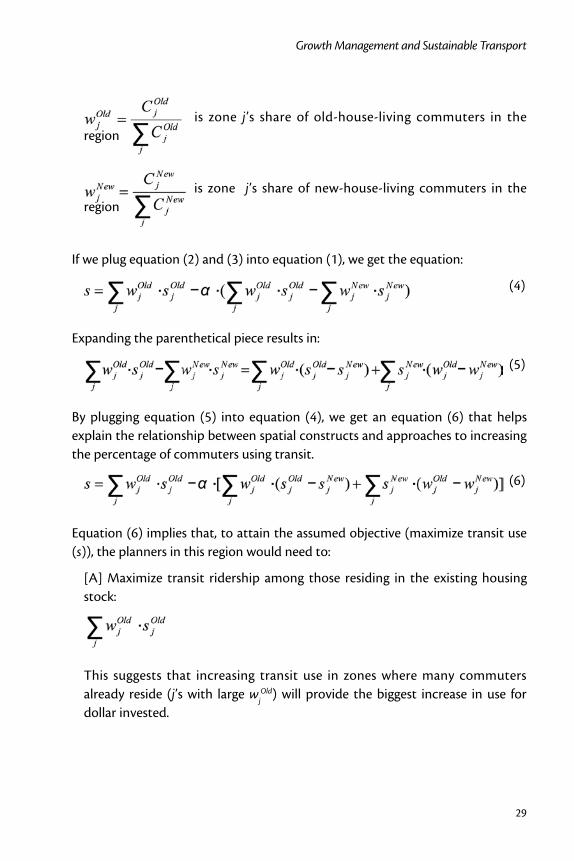
is zone j’s share of old-house-living commuters in the region
is zone j’s share of new-house-living commuters in the region
If we plug equation (2) and (3) into equation (1), we get the equation:
(4)
Expanding the parenthetical piece results in:
(5)
By plugging equation (5) into equation (4), we get an equation (6) that helps explain the relationship between spatial constructs and approaches to increasing the percentage of commuters using transit.
(6)
Equation (6) implies that, to attain the assumed objective (maximize transit use (s)), the planners in this region would need to:
[A] Maximize transit ridership among those residing in the existing housing stock:
This suggests that increasing transit use in zones where many commuters already reside (j’s with large wj
Old) will provide the biggest increase in use for dollar invested.
Journal of Public Transportation, Vol. 12, No. 4, 2009
30
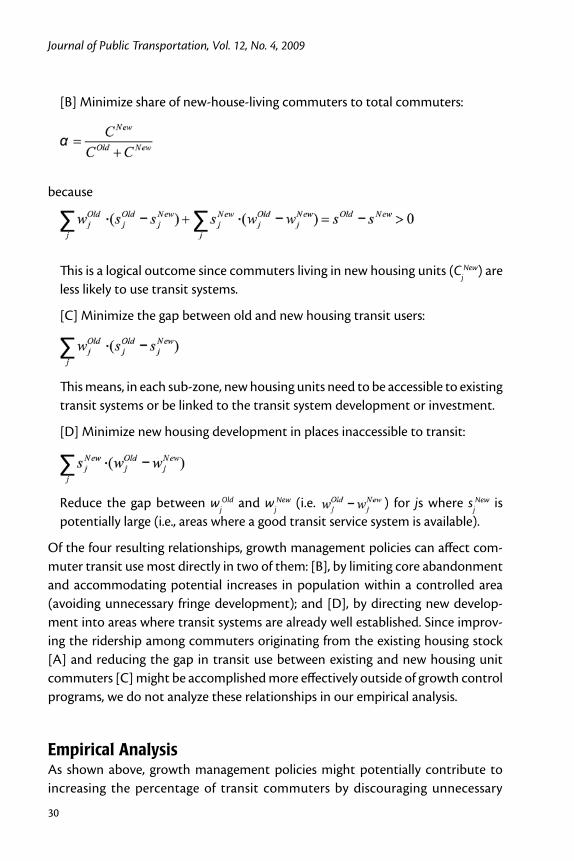
[B] Minimize share of new-house-living commuters to total commuters:
because
This is a logical outcome since commuters living in new housing units (CjNew) are
less likely to use transit systems.
[C] Minimize the gap between old and new housing transit users:
This means, in each sub-zone, new housing units need to be accessible to existing transit systems or be linked to the transit system development or investment.
[D] Minimize new housing development in places inaccessible to transit:
Reduce the gap between wj
Old and wjNew (i.e. ) for js where sj
New is potentially large (i.e., areas where a good transit service system is available).
Of the four resulting relationships, growth management policies can affect com-muter transit use most directly in two of them: [B], by limiting core abandonment and accommodating potential increases in population within a controlled area (avoiding unnecessary fringe development); and [D], by directing new develop-ment into areas where transit systems are already well established. Since improv-ing the ridership among commuters originating from the existing housing stock [A] and reducing the gap in transit use between existing and new housing unit commuters [C] might be accomplished more effectively outside of growth control programs, we do not analyze these relationships in our empirical analysis.
Empirical AnalysisAs shown above, growth management policies might potentially contribute to increasing the percentage of transit commuters by discouraging unnecessary
31
Growth Management and Sustainable Transport
new development and directing a higher proportion of new development into the areas where transit systems are already established. The critical question then is—are they working? Are growth management policies effective in increasing transit ridership? In this section, we try to determine whether or not contempo-rary growth management policies are effectively contributing to increasing the percentage of commuters using transit and through what causal mechanisms. We look at this question by statistically comparing three indicators in regions that are contained within growth management states with regions that are not to see if variations in transit ridership exist.
IndicatorsOur first regional transit use indicator is simply a measurement of the change in the percentage of commuters that use transit (Δs) from 2000 to 2005. The com-parison will help determine whether regions that are contained within growth management states show a discernable difference in transit use over the areas without similar policies.
Although a statistically significant Δs will help describe the differences between growth management areas and non-growth management areas, it may not be useful in discerning how the change (positive or negative) might be achieved. Based on our previous analytical framework, we are most interested in whether the change is due to limiting core abandonment and accommodating potential increases in population within a controlled area (avoiding unnecessary fringe development) and by directing new development into areas where transit systems exist. These questions require an analysis of occupancy rate change and an analysis on the location of new developments.
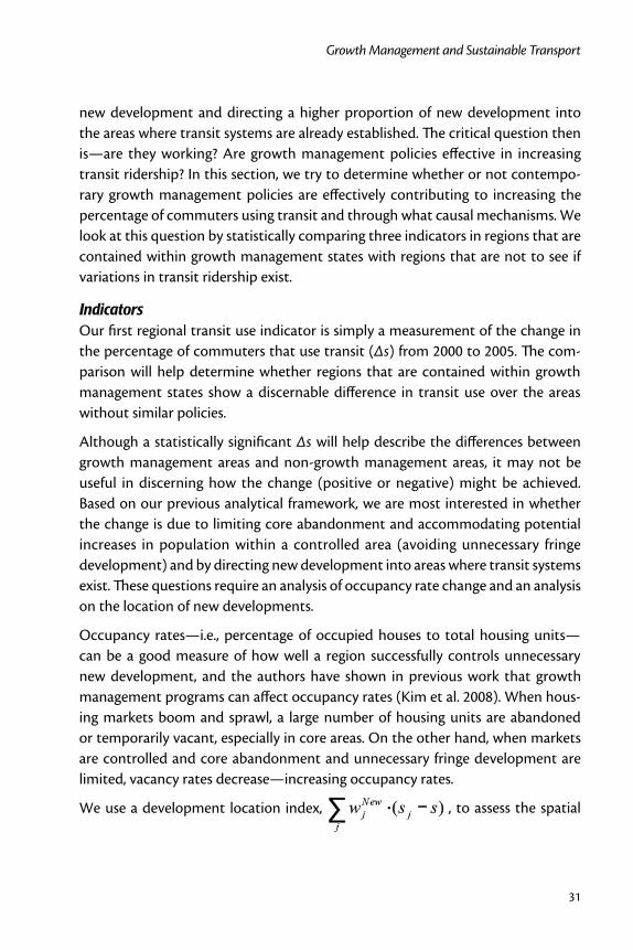
Occupancy rates—i.e., percentage of occupied houses to total housing units—can be a good measure of how well a region successfully controls unnecessary new development, and the authors have shown in previous work that growth management programs can affect occupancy rates (Kim et al. 2008). When hous-ing markets boom and sprawl, a large number of housing units are abandoned or temporarily vacant, especially in core areas. On the other hand, when markets are controlled and core abandonment and unnecessary fringe development are limited, vacancy rates decrease—increasing occupancy rates.
We use a development location index, , to assess the spatial
Journal of Public Transportation, Vol. 12, No. 4, 2009
32
distribution of new development in a region, in this case, whether or not it occurs in transit ready areas. When an increasingly large proportion of new develop-ment—i.e., a large wj—occurs in an area where transit use is lower than the regional average—i.e., negative (sj – s)—the index will be negative. In contrast, when new development is directed into areas with a positive (sj – s), areas of higher transit use percentages, the index will be positive. Although not part of this work, tracking an index of this kind over time would help determine if growth is being directed to established transit areas.
Data SourcesFor this work, we use a number of data sets, including the 2005 American Com-munity Survey (ACS) and their Public Use Microdata Samples (PUMS), along with the U.S. Census Bureau decennial census of 2000. The PUMS provides sampled data on a wide range of information on housing units including the year of con-struction and resident commuting mode. It also informs on the location of the sampled housing units by Public Use Microdata Area (PUMA), which are generally sub-regional zones within Metropolitan Statistical Areas (MSAs) or Primary Met-ropolitan Statistical Areas (PMSA). The 2005 ACS PUMS data enable us to derive new development location indexes for individual regions.
Study AreasOur geographies consist of individual MSAs as defined by U.S. Office of Manage-ment and Budget in 1999 and used for the 2000 census. In the case of very large metropolitan areas classified as Consolidated Metropolitan Statistical Areas (CMSAs), the PMSAs within the CMSAs are regarded as the unit of analysis. In terms of growth management and planning policies in general, PMSAs more con-sistently reflect governance and potential policy enforcement geographies.
Among the more than 300 MSAs and PMSAs available, the 103 regions containing populations of more than 500,000 in the year 2000 are selected. Because MSA or PMSA boundaries are not exactly matched with PUMA boundaries, we redefined the geographic boundaries of some of the regions by adding adjacent counties to the existing 1999 definition. A boundary redefinition is not workable in four regions—the Hartford MSA, the Boston-Worcester-Lawrence CMSA, the Denver-Boulder-Greeley CMSA, and the New York-Northern New Jersey-Long Island CMSA—and are not considered in this study. There are also four regions that straddle both growth management and non-growth management states—the Philadelphia-Wilmington-Atlantic City CMSA, the Wilmington-Newark PMSA, the Providence-Fall River-Warwick MSA, and the Washington-Baltimore CMSA; these regions are
33
Growth Management and Sustainable Transport
also excluded from consideration. Of the original 103 eligible MSAs or PMSAs, 95 are used this analysis; 16 of them are within growth management states, while the remaining 79 are outside of any growth management states.
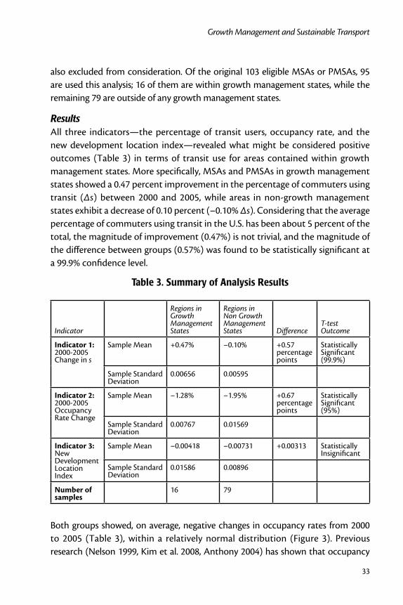
ResultsAll three indicators—the percentage of transit users, occupancy rate, and the new development location index—revealed what might be considered positive outcomes (Table 3) in terms of transit use for areas contained within growth management states. More specifically, MSAs and PMSAs in growth management states showed a 0.47 percent improvement in the percentage of commuters using transit (Δs) between 2000 and 2005, while areas in non-growth management states exhibit a decrease of 0.10 percent (–0.10% Δs). Considering that the average percentage of commuters using transit in the U.S. has been about 5 percent of the total, the magnitude of improvement (0.47%) is not trivial, and the magnitude of the difference between groups (0.57%) was found to be statistically significant at a 99.9% confidence level.
Table 3. Summary of Analysis Results
Indicator
Regions in Growth Management States
Regions inNon Growth Management States Difference
T-test Outcome
Indicator 1: 2000-2005 Change in s
Sample Mean +0.47% –0.10% +0.57 percentage points
Statistically Significant (99.9%)
Sample Standard Deviation
0.00656 0.00595
Indicator 2: 2000-2005 Occupancy Rate Change
Sample Mean –1.28% –1.95% +0.67 percentage points
Statistically Significant (95%)
Sample Standard Deviation
0.00767 0.01569
Indicator 3: New Development Location Index
Sample Mean –0.00418 –0.00731 +0.00313 Statistically Insignificant
Sample Standard Deviation
0.01586 0.00896
Number of samples
16 79
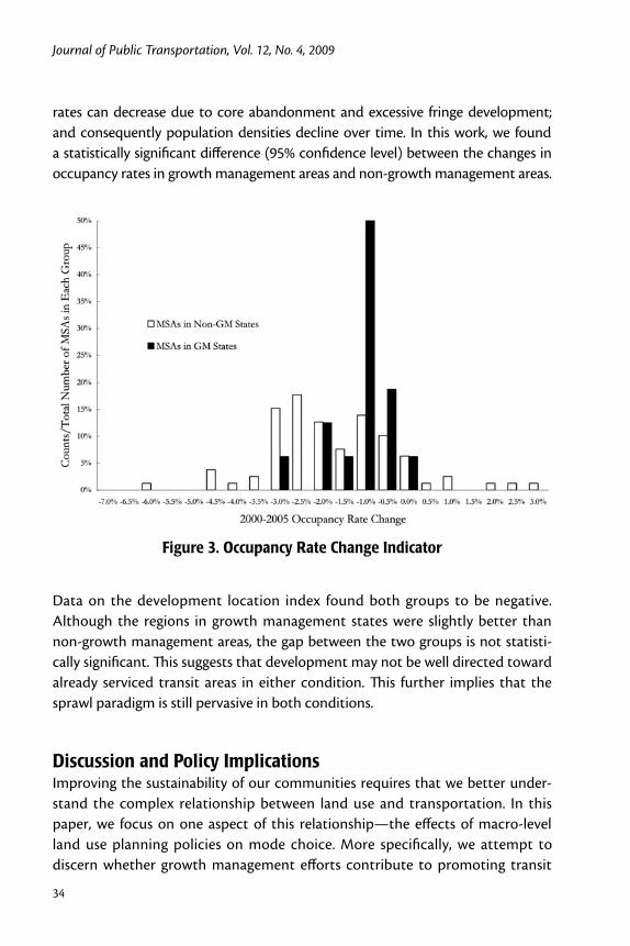
Both groups showed, on average, negative changes in occupancy rates from 2000 to 2005 (Table 3), within a relatively normal distribution (Figure 3). Previous research (Nelson 1999, Kim et al. 2008, Anthony 2004) has shown that occupancy
Journal of Public Transportation, Vol. 12, No. 4, 2009
34
rates can decrease due to core abandonment and excessive fringe development; and consequently population densities decline over time. In this work, we found a statistically significant difference (95% confidence level) between the changes in occupancy rates in growth management areas and non-growth management areas.
Figure 3. Occupancy Rate Change Indicator
Data on the development location index found both groups to be negative. Although the regions in growth management states were slightly better than non-growth management areas, the gap between the two groups is not statisti-cally significant. This suggests that development may not be well directed toward already serviced transit areas in either condition. This further implies that the sprawl paradigm is still pervasive in both conditions.
Discussion and Policy ImplicationsImproving the sustainability of our communities requires that we better under-stand the complex relationship between land use and transportation. In this paper, we focus on one aspect of this relationship—the effects of macro-level land use planning policies on mode choice. More specifically, we attempt to discern whether growth management efforts contribute to promoting transit

35
Growth Management and Sustainable Transport
use and, if so, through what causal mechanisms. We looked at 95 metropolitan areas across the U.S.—16 within and 79 outside of growth management program jurisdiction. We found that MSAs and PMSAs that areas contained within growth management jurisdictions showed a statistically significant improvement in the percentage of commuters using transit. This is consistent with previous studies (Nelson 1999, Porter et al. 2005) and helps support an argument that growth management efforts can contribute to reducing auto-dependency and promote more sustainable transport. We argue that, theoretically, the causal relationships between growth management policies and the noted increase in commuter tran-sit use might be derived in several ways, including limiting core abandonment and accommodating potential increases in population within a controlled area and directing new development into areas where transit systems are already well established.
We found a statistically significant gap in occupancy rate, with higher rates in the growth management regions, implying good control over unnecessary new devel-opment. But there was little statistical support that new development was taking place in transit accessible areas. This implies that the improvement in transit use might be due mainly to increased occupancy rather than a structural shift in locat-ing new development to areas already serviced. It might be argued that an increase in occupancy (especially in areas already well serviced by transit) is an important and low-cost first step that must take place before any tangible change in com-munity structure can be realized. And, as many growth management programs are relatively new (as compared to other programs), they might not yet be mature enough to exhibit these adaptations.
Another potential explanation for the lack of locational reordering might be an imperfect integration of growth management policies with transportation plan-ning and investment decision making. Many growth management programs only loosely define areas where new development might be advantageous to their com-munities rather than actively encouraging development in transit-ready areas or new-transit-investment sites.
Finally, we think that additional explanations for the observed relationships might exist, particularly the connection between land use and transportation planning decisions at the local level. In fact, micro level considerations may go further in explaining the nature of our observed relationships than the state-level growth management policies. Our ongoing work focuses on seeking these relationships. We also think, however, that this paper is an important and timely step in the
Journal of Public Transportation, Vol. 12, No. 4, 2009
36
discourse on state-level land use policies. As governments increasingly search for more sustainable choices in spite of falling and failing budgets, investment deci-sions become more critically scrutinized. In our opinion, public transportation infrastructure is one such choice that also needs coherent policies that support long-range sustainability and adequate use of that infrastructure in order to be successful. Many of these policies will be borne from state level growth manage-ment policies.
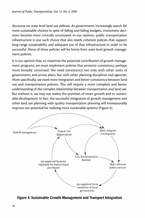
It is our opinion that, to maximize the potential contribution of growth manage-ment programs, we must implement policies that promote consistency, perhaps more broadly construed. We need consistency not only with other units of governments and across plans, but with other planning disciplines and agencies. More specifically, we need more integration and better consistency between land use and transportation policies. This will require a more complete and better understanding of the complex relationship between transportation and land use. But without it, we may not realize the promises of smart growth and or sustain-able development. In fact, the successful integration of growth management and other land use planning with quality transportation planning will immeasurably improve our potential for realizing more sustainable systems (Figure 4).
Figure 4. Sustainable Growth Management and Transport Integration
37
Growth Management and Sustainable Transport
References
Anthony, J. 2004. Do state growth management regulations reduce sprawl? Urban Affairs Review 39(3): 376–397.
Badoe, D. A., and E. J. Miller. 2000. Transportation-land-use interaction: Empirical findings in North America and their implications for modeling Transportation Research Part D 5(4): 235–263.
Banister, D. 2008. The sustainable mobility paradigm. Transport Policy 15(2): 73–80.
Black, W. R. 2000. Socio-economic barriers to sustainable transport. Journal of Transport Geography 8(2): 141–147.
Carruthers, J. I. 2002. The impacts of state growth management programmes: A comparative analysis. Urban Studies 39(11): 1959–1982.
Daly, H. E. 1996. Beyond Growth: The Economics of Sustainable Development. Bea-con Press, Boston.
Dawkins, C. J., and A. C. Nelson. 2003. State growth management programs and central-city revitalization. Journal of the American Planning Association 69(4): 381–396.
Deakin, E. 2002. Sustainable transportation: U.S. dilemmas and European experi-ences. Transportation Research Record 1792: 1–11.
Gale, D. E. 1992. Eight state-sponsored growth management programs: A compar-ative analysis. Journal of the American Planning Association 58(4): 425–439.
Hawken, P. A., and L. H. Lovins. 1999. Natural Capitalism: Creating the Next Indus-trial Revolution. Little Brown and Company, Boston.
Holden, E., and I. T. Norland. 2005. Three challenges for the compact city as a sustainable urban form: Household consumption of energy and transport in eight residential areas in the Greater Oslo Region. Urban Studies 42(12): 2145–2166.
Hull, A. 2008. Policy integration: What will it take to achieve more sustainable transport solutions in cities? Transport Policy 15(2): 94–103.
Jabareen, Y. R. 2006. Sustainable urban forms: Their typologies, models and con-cepts. Journal of Planning Education and Research 26(1): 38–52.
Journal of Public Transportation, Vol. 12, No. 4, 2009
38
Jun, M. 2004. The effects of Portland’s urban growth boundary on urban develop-ment patterns and commuting. Urban Studies 41(7): 1333–1348.
Kim, J. H., and B. Deal. 2008. Toward compact development? The limitations of contemporary state-level growth management in the U.S. Presented at 4th ACSP-AESOP Joint Congress, Chicago.
Knaap, G. J., and A. Chakraborty. 2007. Comprehensive planning for sustainable rural development.” Journal of Regional Analysis and Policy 37 (2): 18-20
Litman, T., and D. Burwell. 2006. Issues in sustainable transportation. International Journal of Global Environmental Issues 6(4): 331–347.
Litman, T. 2007. Developing indicators for comprehensive and sustainable trans-port planning. Transportation Research Record 2017: 10–15.
May, A.D., A. F. Jopson, and B. Matthews. 2003. Research challenges in urban trans-port policy. Transport Policy 10(3): 157–164.
May, T., and M. Crass. 2007. Sustainability in transport: Implications for policy makers. Transportation Research Record 2017: 1–9.
Nelson, A. C. 1999. Comparing states with and without growth management: Analysis based on indicators with policy implications. Land Use Policy 16(2): 121–127.
Nelson, A. C., R. Pendall, C. J. Dawkins, and G. J. Knaap. 2004. The link between growth management and housing affordability: The academic evidence. In Growth Management and Affordable Housing: Do They Conflict? Brookings Institution Press, Washington D.C.
Oregon Land Conservation and Development Commission. 1991. Transportation Planning Rule. http://www.oregon.gov/LCD/TGM/policies.shtml Accessed July 28 2008.
Parsons Brinckerhoff Quade and Douglas Inc. 1996. Transit and Urban Form. Tran-sit Cooperative Research Program Report 16, Transportation Research Board, National Research Council, Washington D.C.
Porter, C. D., B. T. Siethoff, and V. Smith. 2005. Impacts of comprehensive plan-ning and smart growth initiatives on transportation. Transportation Research Record 1902: 91–98.
39
Growth Management and Sustainable Transport
Porter, D. R. 1996. State framework laws for guiding urban growth and conserva-tion in the United States. Pace Environmental Law Review 13(2): 547–560.
Richardson, B. C. 1999. Toward a policy on a sustainable transportation system. Transportation Research Record 1670: 27–34.
Richardson, B. C. 2005. Sustainable transport: Analysis frameworks. Journal of Transport Geography 13 (1): 29–39.
Sierra Club. 1999. Solving sprawl: The Sierra Club rates the states. http://www.sier-raclub.org/sprawl/ report99/ Accessed March 20 2008.
Transportation Research Board. 1997. Toward a sustainable future: Addressing the long-term effects of motor vehicle transportation on climate and ecol-ogy. Special Report 251, Transportation Research Board, National Research Council, Washington, D.C.
Weitz, J. 1999. From quiet revolution to smart growth: State growth management programs 1960 to 1999. Journal of Planning Literature 14(2): 267–338.
About the Authors
Brian Deal ([email protected]) is an assistant professor of urban and regional planning, Director of the LEAM modeling laboratory, and the Director of the Smart Energy Design Assistance Center at the University of Illinois. At LEAM, he takes an innovative approach to analyzing the potential environmental implications of regional land use decisions through dynamic spatial simulation modeling. He teaches multi-disciplinary sustainable design studio/workshops and seminar courses, physical planning, on-line courses that contribute toward a certification program in sustainable design, and professional development courses on sustainability.
Jae Hong Kim ([email protected]) is a PhD Candidate in regional planning at the University of Illinois at Urbana-Champaign. His work seeks to understand the dynamic interrelationship between the progress of a regional economic system and the evolution of its spatial structure, assessing the validity, timeliness, and effective-ness of various land use, transportation, and economic development policies. As a research assistant, he has been engaged in regional economic analysis and land use modeling projects for REAL and LEAM laboratories.
Arnab Chakraborty ([email protected]) is an assistant professor of urban and regional planning at the University of Illinois at Urbana-Champaign. He has orga-
Journal of Public Transportation, Vol. 12, No. 4, 2009
40
nized and led large-scale, scenario planning processes in the past. His dissertation focused on connecting simple assessment modeling techniques with stakeholder driven planning processes that contributed, in part, in shaping the state govern-ment’s land use policy agenda in Maryland. He currently leads a project at the LEAM lab for analyzing alternative policy-based scenarios for Maryland and teaches plan making, communications, and growth management and regional planning.
41
Bike-sharing
Bike-sharing: History, Impacts, Models of Provision, and Future
Paul DeMaio MetroBike, LLC
Abstract
This paper discusses the history of bike-sharing from the early 1st generation program to present day 3rd generation programs. Included are a detailed examination of models of provision, with benefits and detriments of each, and a description of capital and operating costs. The paper concludes with a look into the future through discus-sion about what a 4th generation bike-sharing program could be.
IntroductionBike-sharing, or public bicycle programs, have received increasing attention in recent years with initiatives to increase cycle usage, improve the first mile/last mile connection to other modes of transit, and lessen the environmental impacts of our transport activities. Originally a concept from the revolutionary 1960s, bike-sharing’s growth had been slow until the development of better methods of tracking bikes with improved technology. This development gave birth to the rapid expansion of bike-sharing programs throughout Europe and now most other continents during this decade.
Since the publication of “Will Smart Bikes Succeed as Public Transportation in the United States?” (DeMaio 2004), much has happened in the nascent field of bike-sharing. While the previous paper discussed the conditions for a success-ful program, this paper discusses the history of bike-sharing, provides a detailed
Journal of Public Transportation, Vol. 12, No. 4, 2009
42
examination of models of provision with benefits and detriments of each, exam-ines capital and operating expenses, and concludes with a look into the future of bike-sharing through a discussion about what a 4th generation bike-sharing program could be.
History of Bike-sharingThere have been three generations of bike-sharing systems over the past 45 years (DeMaio 2003, 2004). The 1st generation of bike-sharing programs began on July 28, 1965, in Amsterdam with the Witte Fietsen, or White Bikes (Schimmelpennick 2009). Ordinary bikes, painted white, were provided for public use. One could find a bike, ride it to his or her destination, and leave it for the next user. Things did not go as planned, as bikes were thrown into the canals or appropriated for private use. The program collapsed within days.
In 1991, a 2nd generation of bike-sharing program was born in Farsø and Grenå, Denmark, and in 1993 in Nakskov, Denmark (Nielse 1993). These programs were small; Nakskov had 26 bikes at 4 stations. It was not until 1995 that the first large-scale 2nd generation bike-sharing program was launched in Copenhagen as Bycyklen, or City Bikes, with many improvements over the previous generation. The Copenhagen bikes were specially designed for intense utilitarian use with solid rubber tires and wheels with advertising plates, and could be picked up and returned at specific locations throughout the central city with a coin deposit. While more formalized than the previous generation, with stations and a non-profit organization to operate the program, the bikes still experienced theft due to the anonymity of the user. This gave rise to a new generation of bike-sharing with improved customer tracking.
The first of this new breed of 3rd generation bike-sharing programs was Bikeabout in 1996 at Portsmouth University in England, where students could use a magnetic stripe card to rent a bike (Black and Potter undated). This and the following 3rd generation of bike-sharing systems were smartened with a variety of technologi-cal improvements, including electronically-locking racks or bike locks, telecom-munication systems, smartcards and fobs, mobile phone access, and on-board computers.
Bike-sharing grew slowly in the following years, with one or two new programs launching annually, such as Rennes’ (France) Vélo à la Carte in 1998 and Munich’s Call a Bike in 2000, but it was not until 2005 when 3rd generation bike-sharing
43
Bike-sharing
took hold with the launch of Velo’v, with 1,500 bikes in Lyon by JCDecaux (Opti-mising Bike Sharing in European Cities 2009a, 2009b, 2009c). This was the largest 3rd generation bike-sharing program to date and its impact was noticeable. With 15,000 members and bikes being used an average of 6.5 times each day by late 2005, Lyon’s big sister, Paris, took notice (Henley 2005).
Two years later, Paris launched its own bike-sharing program, Vélib’, with about 7,000 bikes, which has expanded to 23,600 bikes in the city and suburbs since. This massive undertaking and its better-than-expected success changed the course of bike-sharing history and generated enormous interest in this transit mode from around the world. Outside Europe, bike-sharing finally began to take hold in 2008, with new programs in Brazil, Chile, China, New Zealand, South Korea, Taiwan, and the U.S. Each was the first 3rd generation bike-sharing program for the countries.
By the end of 2007, there were about 60 3rd generation programs globally (DeMaio 2007). By the end of 2008, there were about 92 programs (DeMaio 2008a). Cur-rently, there are about 120 programs, as shown in Figure 1, with existing 3rd gen-eration programs shown with a cyclist icon and planned programs shown with a question mark icon (MetroBike 2009).
Bike-sharing’s ImpactsBike-sharing has had profound affects on creating a larger cycling population, increasing transit use, decreasing greenhouse gases, and improving public health. It has had the affect of raising bike mode share between 1.0 - 1.5 percent in cities with pre-existing low cycling use. Cycle mode share in Barcelona was 0.75 per-cent in 2005 and increased to 1.76 percent in 2007, the year Bicing was launched (Romero 2008). In Paris, cycle mode share increased from about 1 percent in 2001 to 2.5 percent in 2007, the year Vélib’ was launched (Nadal 2007; City of Paris 2007). Cycle facility improvements were made in both cities during these time periods; however, it is difficult to extract the affects the new facilities had on cycle use.
Transit use increases in cities with bike-sharing due to the new bike transit trips, improved connectivity to other modes of transit due to the first mile/last mile solution bike-sharing helps solve, and decreased personal vehicle trips. While bike-sharing trips do replace some trips previously made on other modes of transit (50 percent in the case of Velo’v in Lyon), “[t]he loss of customers for public transport services is quite low as many users are still holders of a public transport pass”
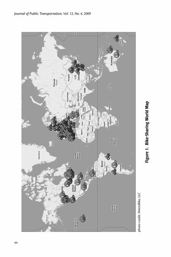
Journal of Public Transportation, Vol. 12, No. 4, 2009
44
phot
o cr
edit
: Met
roBi
ke, L
LC
Figu
re 1
. Bi
ke-S
hari
ng W
orld
Map
45
Bike-sharing
(NICHES 2007). The City of Paris reported 50 million trips made by Vélib’ in its first two years. In 2008, 28 percent of the survey respondents were less likely to use their personal vehicle; in 2009, this increased to 46 percent. In 2008, 21 percent of survey respondents used Vélib’ to reach the subway, train, or bus, and 25 percent used Vélib’ on the return trip from other transit modes. In 2009, 28 percent used Vélib’ to begin and to end their multi-leg transit trip (City of Paris 2008, 2009).
Many bike-sharing programs take pride in their environmental contribution. Montreal’s Bixi proudly states that its program has saved over 3,000,000 pounds of greenhouse gases since inception in May 2009 (Bixi 2009a). Lyon states that its program, which launched in 2005, has saved the equivalent of 18,600,000 pounds of CO2 pollution from the atmosphere (Greater Lyon 2009). The public health benefits of bike-sharing have yet to be analyzed; however, the health benefits of cycling are well-known (Andersen et al. 2000; Cavill and Davis 2006; Shepard 2008).
Models of ProvisionSince bike-sharing’s inception, various models of provision have existed (Büh-rmann 2008). As illustrated in Figure 2, bike-sharing providers have included governments, quasi-governmental transport agencies, universities, non-profits, advertising companies, and for-profits. This section discusses the benefits and detriments of each model.
In the government model, the locality operates the bike-sharing service as it would any other transit service. The government of Burgos, Spain, purchased and oper-ates an off-the-shelf bike-sharing system called Bicibur (Civitas 2009). With this model, the government as operator has greater control over the program. On the other hand, it may not have the experience that existing bike-sharing operators have in managing a program. Also, the government maintains the liability for the program, which can be less desirable from a government’s perspective.
The transport agency model has a quasi-governmental organization providing the service. The transport agency’s customer is a jurisdiction, region, or nation. Transport agencies, such as Deutsche Bahn of Germany and Stationnement de Montréal, are prime examples. Deutsche Bahn is the national railway provider of Germany and operates a car-sharing and Call a Bike bike-sharing service. Station-nement de Montréal, the parking authority of Montréal, provides “management of municipal paid on-street and off-street parking” and the Bixi bike-sharing
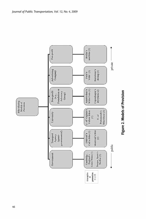
Journal of Public Transportation, Vol. 12, No. 4, 2009
46
Figu
re 2
. Mod
els
of P
rovi
sion
47
Bike-sharing
service. Both organizations have gotten into bike-sharing as an extension of their other transport offerings to be a well-rounded mobility provider (Deutsche Bahn 2009; Stationnement de Montréal 2009).
The benefit of the quasi-government transport agency model is that the jurisdic-tion benefits from the experience and innovation of the bike-sharing service pro-vider, especially in the case of national Deutsche Bahn, without needing to develop the capabilities internally. Additionally, both the jurisdiction and transport agency’s top priority is to provide a useful transit service, rather than generating revenues, which is discussed in more detail below as a detriment in the advertising company and for-profit models. A detriment of this model is that, without the locality releasing a tender for the service, a more qualified operator may exist than the transport agency operator.
The university model has the educational institution providing the service, most likely in a campus setting. Examples are the former program at the University of Portsmouth, England, and newer incarnations such as that of St. Xavier University in Chicago (Black and Potter undated; DeMaio 2008b). The benefit of this model is the university can expand its intra-campus transit service without relying on the jurisdiction to offer sufficient bike-sharing service on campus. A detriment is the surrounding jurisdiction potentially would not benefit from the service unless it was opened to the adjacent neighborhoods. Also, if the locality were to use another system, there could be compatibility issues with the university’s system.
The non-profit model has an organization which was either expressly created for the operation of the service or one that folds the bike-sharing service into its exist-ing interests. Examples of non-profit programs include the City Bike Foundation of Copenhagen, which operates Bycyklen, and the Nice Ride Minnesota program in Minneapolis (City Bike Foundation of Copenhagen undated; Nice Ride Minnesota 2009). While the non-profit operates the program, it usually receives funding from the jurisdiction for the service it provides to the public in addition to collecting the revenues generated by membership and usage fees and sponsorships (Nice Ride Minnesota 2009). The non-profit model benefits the locality as it removes liability from it and places the liability on the non-profit which has limited funding and is less likely to be sued. A detriment of this model is the non-profit can be reliant on the public sector for a majority of its funding (Nice Ride Minnesota 2009).
With the advertising company model, companies such as JCDecaux, Clear Chan-nel Outdoor, and Cemusa offer a bike-sharing program to a jurisdiction, usually in exchange for the right to use public space to display revenue-generating adver-
Journal of Public Transportation, Vol. 12, No. 4, 2009
48
tisements on billboards, bus shelters, and kiosks. The benefit of this model is it can be convenient and cost-effective for local governments that could not afford to provide the bike-sharing service otherwise. To date, this model has been the most popular. A detriment with the advertising company model is the problem of moral hazard. The advertising company usually does not benefit from revenues generated by the system, as the revenues usually go to the jurisdiction, so the advertising company may not have the same incentive to operate the program as if the revenues were directly related to their level of service, regardless of what they agreed to in a service contract. This is highlighted in Paris by the statement by the director general of JCDecaux that its contract with Paris is unsustainable due to the unexpectedly high level of theft and vandalism the program has experienced: “It’s simple. All the receipts go to the city. All the expenses are ours” (BBC 2009).
In one case in particular, the advertising company provides the bike-sharing service for a fee and not for an advertising contract. In Barcelona, B:SM (Barce-lona de Serveis Municipals), a company owned by the city, has contracted with Clear Channel Outdoor to operate the service (Barcelona de Serveis Municipals undated). This model is more similar to the transport provider model, as the con-tractor happens to be an advertising company but its advertising services are not used.
In the for-profit model, a private company provides the service with limited or no government involvement. Nextbike is a prime example of this model, with a local business running the service in a locality with the off-the-shelf flexible station sys-tem. While similar to the advertising company model, this model differs as there is no on-street advertising contract with the locality and the for-profit keeps all revenues generated. A benefit of this model is that the private sector can start a service as an entrepreneurial activity rather than wait for the public sector to do so. A detriment is that the for-profit may not receive funding assistance for the service as do programs offered under other models. Additionally, if the for-profit uses a fixed, versus flexible, system, they would need to have the locality’s support to use public space, unless all stations are on private property.
There is no one ideal model that works best in all jurisdictions. There are factors that affect which models can be used and include the size of the jurisdiction and availability of both bike-sharing systems able to operate in the country and local entrepreneurs to run the program. The size of a jurisdiction is an important factor, as the predominant model of advertising companies providing bike-sharing ser-
49
Bike-sharing
vice tends to be mostly in larger cities where the potential for views of advertising, and therefore advertising revenue, is the greatest.
Demand for bike-sharing has been around longer in Europe than in other con-tinents, and the bike-sharing industry has grown more quickly, which has led to a more rapid growth of programs in European countries. From the continent to the national level, home-grown systems generally dominate in the countries in which they are headquartered. For example, Bicincitta’ is headquartered in Italy and has the majority of programs offered there. Both Call a Bike and nextbike are headquartered in Germany and have the majority of programs there. The German government’s subsidization of Deutsche Bahn, which offers the Call a Bike service, also has an effect on its growth nationally.
CostsThe capital and annual operating costs of programs vary greatly, depending on the system, population density, service area, and fleet size. Capital costs include fabrication of the bikes and stations, license or purchase of the back-end system used to operate the equipment, member access cards (if necessary), purchase or rental of maintenance and distribution vehicles, and installation. Clear Channel Outdoor’s SmartBike system is estimated to have capital costs of around $3,600 per bicycle; JCDecaux’s Cyclocity system is estimated at $4,400 per bicycle; and Bixi is estimated to be $3,000 per bicycle (New York City Department of City Planning 2009). Nice Ride Minnesota is planning to launch in 2010 using Bixi and estimates $3,200 per bike (Twin Cities Bike Share 2008).
Operating costs include maintenance, distribution, staff, insurance, office space, storage facilities, website hosting and maintenance, and electricity (if necessary). New York City’s analysis of several systems concludes an average operating cost of about $1,600 per bicycle (New York City Department of City Planning 2009). Minneapolis expects the same (Twin Cities Bike Share 2008).
Bike-sharing’s 4th GenerationWhat will the 4th generation of bike-sharing look like? As the 3rd generation of bike-sharing brought about smartening of the concept with smartcards, mobile phones, and kiosks with screens, the hallmark of the 4th generation will be improved efficiency, sustainability, and usability. This is being accomplished by

Journal of Public Transportation, Vol. 12, No. 4, 2009
50
improving distribution of bikes, installation, powering of stations, tracking, offer-ing pedalec (pedal assistance) bikes, and new business models.
Improved DistributionDistribution of bikes must improve to make the bike-sharing service more efficient and environmentally friendly. Staff moving bikes from areas of high supply/low demand to areas of low supply/high demand is time consuming, expensive, and polluting. Programs will create “push” and “pull” stations which will either encour-age trips to leave or arrive, respectively, at these stations based on the demand for bikes. Incentives will include free time, credit, or cash.
Vélib’ has made an improvement in this area with the launch of its “V+” concept, reports Velib et Moi - Le Blog. As it requires more physical effort and time for cus-tomers to reach uphill stations, V+ gives an extra 15 minutes to access about 100 of these designated uphill stations. The extra time given has encouraged greater use of these stations. Within the first three months of V+ being offered in Summer 2008, 314,443 instances of 15-minute credits were given. These extra 15-minute bonuses also may be saved up when not used during the trip to the V+ station (Vélib’ 2008). Free bike-on-transit capabilities adjacent to specific stations could also assist in pushing bikes uphill where bike-sharers could board another mode of transit. Luud Schimmelpennick, a co-inventor of the bike-sharing concept, reports the operational cost of JCDecaux’s distribution of bicycles is about $3 each (Schim-melpennick 2009). He believes paying customers for distribution to stations that need more bikes, either through providing a customer credit towards future use or paying the customer outright, would increase distribution efficiency at a fraction of the present cost.
Ease of InstallationInstalling a station takes time and is costly, with removal of asphalt or pavers, undergrounding of the structure and wires, hook-up to a nearby electrical source, and replacement of building materials. Public Bike System has limited this expense with its “technical platform,” which is the bike-sharing station’s base and houses the wires for its bike dock and pay station. The technical platform is placed on the ground without need for construction, as its weight and minimal bolting to the ground are sufficient to keep it in place (Public Bike System undated) (see Figure 3).
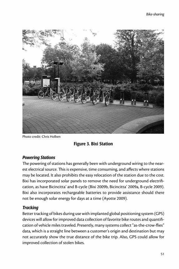
51
Bike-sharing
Photo credit: Chris Holben
Figure 3. Bixi Station
Powering StationsThe powering of stations has generally been with underground wiring to the near-est electrical source. This is expensive, time consuming, and affects where stations may be located. It also prohibits the easy relocation of the station due to the cost. Bixi has incorporated solar panels to remove the need for underground electrifi-cation, as have Bicincitta’ and B-cycle (Bixi 2009b, Bicincitta’ 2009a, B-cycle 2009). Bixi also incorporates rechargeable batteries to provide assistance should there not be enough solar energy for days at a time (Ayotte 2009).
TrackingBetter tracking of bikes during use with implanted global positioning system (GPS) devices will allow for improved data collection of favorite bike routes and quantifi-cation of vehicle miles traveled. Presently, many systems collect “as-the-crow-flies” data, which is a straight line between a customer’s origin and destination but may not accurately show the true distance of the bike trip. Also, GPS could allow for improved collection of stolen bikes.
Journal of Public Transportation, Vol. 12, No. 4, 2009
52
Pedal AssistanceNot everyone has the leg strength to ride a bike, especially in hilly areas. Pedelec, or electric pedal assistance bikes, will allow those who would not otherwise be physically able, to give bike-sharing a try. Just as buses have added kneeling and wheelchair features to open themselves up to passengers with disabilities, electric pedal assistance moves bike-sharing to a wider audience. A bike-sharing fleet need not be composed entirely of pedalec bikes, but rather a percentage of vehicles for this purpose to lower the barrier for a portion of the population. Systems that use pedalecs are in Genoa and Monaco, both programs of Bicincitta’ (Bicincitta’ 2009b, Avenir du Vehicule Electrique Mediterraneen 2008).
Business ModelAs the demand for bike-sharing increases, the models of provision will continue to experience growth. New bike-sharing system vendors have sprung up in the indus-try and created their own systems, such as nextbike, Bixi, Veloway, and Smoove. Many of these systems have no outdoor advertising component but rather can be purchased by a local operator. These systems are allowing jurisdictions and universities with populations too small to make outdoor advertising profitable or where advertising on public space is prohibited to consider launching their own bike-sharing services.
ConclusionThe future of bike-sharing is clear: there will be a lot more of it. Gilles Vesco, Vice President of Greater Lyon, quotes his mayor when saying, “There are two types of mayors in the world: those who have bike-sharing and those who want bike-sharing.” This certainly seems to be the case as each bike-sharing program creates more interest in this form of transit—call it a virtuous cycle. As the price of fuel rises, traffic congestion worsens, populations grow, and a greater world-wide con-sciousness arises around climate change, it will be necessary for leaders around the world to find new modes of transport and better adapt existing modes to move people in more environmentally sound, efficient, and economically feasible ways. Bike-sharing is evolving rapidly to fit the needs of the 21st century.
References
Andersen, L., P. Schnohr, M. Schroll, and H.O. Hein. 2000. All-cause mortality asso-ciated with physical activity during leisure time, work, sports, and cycling to
53
Bike-sharing
work. Archives of Internal Medicine. 160:1621-1628. http://archinte.ama-ssn.org/cgi/content/full/160/11/1621/.
Avenir du Vehicule Electrique Mediterraneen. 2008. February 28. http://translate.google.com/translate?prev=_t&hl=en&ie=UTF-8&u=http%3A%2F%2Fwww.avem.fr%2Factualite-monaco-des-velos-electriques-en-libre-service-386.html&sl=fr&tl=en&history_state0/.
Ayotte, A. 2009. Conversation with author. July 13.
Barcelona de Serveis Municipals. undated. BSM Organización. http://www.bsmsa.es/index.php?id=10&L=1/.
BBC. 2009. Thefts puncture Paris bike scheme. February 10. http://news.bbc.co.uk/2/hi/europe/7881079.stm/.
B-cycle. 2009. What is B-cycle? http://www.bcycle.com/.
Bicincitta’. 2009a. Gallery. http://bicincitta.com/gallery.asp/.
Bicincitta’. 2009b. Genoa. http://74.125.113.132/translate_c?hl=en&sl=it&u=http://www.bicincitta.com/citta_v3.asp%3Fid%3D33&prev=/search%3Fq%3D%252Bmobike%2B%252Bgenova%26hl%3Den%26client%3Dfirefox-a%26rls%3Dorg.mozilla:en-US:official%26hs%3DX41%26sa%3DG&rurl=translate.google.com&usg=ALkJrhijAARamP_sUSmk_aUVqkTXn000lw/.
Black, C., and S. Potter. Undated. Portsmouth bikeabout: A smart-card bike club scheme. http://www.metrobike.net/index.php?s=file_download&id=11/.
Bixi. 2009a. Overview. http://www.bixisystem.com/bixi_system/overview/.
Bixi. 2009b. Information. http://montreal.bixi.com/home/home-info/.
Bührmann. 2008. Bicycles as public-individual transport – European develop-ments. 18. http://www.metrobike.net/index.php?s=file_download&id=2/.
Cavill, N., and A. Davis. 2006. Cycling and Health. 9-43. http://www.networks.nhs.uk/uploads/07/11/cycling_and_health.pdf/.
City Bike Foundation of Copenhagen. undated. Bycyklen København. http://www.bycyklen.dk/.
City of Paris. 2007. Le Bilan des Deplacements en 2007 a Paris. La Mairie de Paris, L’Observatorie de Deplacements, Paris, France. http://www.paris.fr/portail/
Journal of Public Transportation, Vol. 12, No. 4, 2009
54
deplacements/Portal.lut?page_id=7627&document_type_id=4&document_id=26324&portlet_id=17647&multileveldocument_sheet_id=11982/.
City of Paris. 2008. La lettre Vélib’. May. 10. http://velib.centraldoc.com/newsletter/10_aujourd_hui_nous_vous_connaissons_mieux/.
City of Paris. 2009. La lettre Vélib’. June. 22. http://velib.centraldoc.com/newsletter/22_bientot_2_ans_d_utilisation_votre_regard_sur_le_service/.
Civitas. 2009. City bike scheme in Burgos. http://www.civitas-initiative.org/mea-sure_sheet.phtml?lan=en&id=302/.
DeMaio, P. 2003. Smart bikes: Public transportation for the 21st century. Transpor-tation Quarterly 57(1): 9–11.
DeMaio, P. 2004. Will smart bikes succeed as public transportation in the United States? Journal of Public Transportation 7(2): 1-15.
DeMaio, P. 2007. What a year for bike-sharing. December 30. http://bike-sharing.blogspot.com/2007/12/what-year-for-bike-sharing.html/.
DeMaio, Paul. 2008a. Bike-sharing Wrap-up for 2008. December 31. http://bike-sharing.blogspot.com/2008/12/bike-sharing-wrap-up-for-2008.html/.
DeMaio, P. 2008b. University bike-sharing’s time has come. The Bike-sharing Blog. October 26. http://bike-sharing.blogspot.com/2008/10/university-bike-shar-ings-time-has-come.html/.
Deutsche Bahn. 2009. DB Fuhrpark. http://www.dbfuhrparkservice.de/site/dbfuhrpark/de/anschlussmobilitaet/anschlussmobilitaet.html/.
Greater Lyon. 2009. Velo’v la newsletter. March. 37. http://www.velov.grandlyon.com/Newsletter-Velo-v-numero-37.134.0.html/.
Henley, J. 2005. Rentabike moves up a gear from curiosity to runaway success. The Guardian. August 12. http://www.guardian.co.uk/world/2005/aug/12/france.jonhenley/.
MetroBike. 2009. The Bike-sharing world map. http://maps.google.com/maps/ms?ie=UTF8&hl=en&om=1&msa=0&msid=104227318304000014160.00043d80f9456b3416ced&ll=43.580391,-42.890625&spn=143.80149,154.6875&z=1&source=embed/.

55
Bike-sharing
Nadal, L. 2007. Bike sharing wweeps Paris off its feet. Sustainable Transport. 19. 8 - 12. http://www.itdp.org/documents/st_magazine/ITDP-ST_Magazine-19.pdf/.
New York City Department of City Planning. 2009. Bike-share opportunities in New York City. 84. http://www.nyc.gov/html/dcp/pdf/transportation/bike_share_ complete.pdf/.
NICHES. 2007. Public bicycles. p. 5. http://ange.archangelis.com/typo3/niches/fileadmin/New_folder/Deliverables/D4.3b_5.8_b_PolicyNotes/14397_pn4_public_bikes_ok_low.pdf/.
Nice Ride Minnesota. 2008. Twin Cities bike share project business plan. 38-9. http://www.niceridemn.com/downloads/doc_plan.php/. Nice Ride Minne-sota. 2009. Nice Ride Minnesota. http://www.niceridemn.com/.
Nielse, B. H. 1993. The Bicycle in Denmark: Present Use and Future Potential. Danish Ministry of Transport. 52.
Optimising Bike Sharing in European Cities. 2009a. France. FR_Rennes_Old System tab. http://www.obisproject.com/palio/html.run?_Instance=obis&_PageID=4&_LngID=21&_CatID=722&pic=4&_CheckSum=1012982978/.
Optimising Bike Sharing in European Cities. 2009b. Germany. DE_Berlin tab. http://www.obisproject.com/palio/html.run?_Instance=obis&_PageID=4&_LngID=21&_CatID=722&pic=4&_CheckSum=1012982978/.
Optimising Bike Sharing in European Cities. 2009c. France. FR_Lyon tab. http://www.obisproject.com/palio/html.run?_Instance=obis&_PageID=4&_LngID=21&_CatID=722&pic=4&_CheckSum=1012982978/.
Romero, C. 2008. SpiCycles in Barcelona. Presented to Chamber of Commerce and Industry, December 19, in Bucharest, Romania. 31. http://spicycles.velo.info/Portals/0/FinalReports/Barcelona_Final_Report.ppt/.
Schimmelpennick, L. 2009. Conversation with author. March 5.
Shepard, R. 2008. Is Active Commuting the answer to population health? Sports Medicine. 39(9): 751-758.
Stationnement de Montréal. 2009. Stationnement de Montréal. http://www.stat-demtl.qc.ca/index.php?page_id=42&lang=en/.
Journal of Public Transportation, Vol. 12, No. 4, 2009
56
Stationnement de Montréal. undated. Public Bike System. 15. http://www.metro-bike.net/index.php?s=file_download&id=13/.
Twin Cities Bike Share. 2008. Non-profit business plan for Twin Cities bike share system. December 3. 36 - 44. http://www.niceridemn.com/downloads/doc_plan.php/.
Vélib’. 2008. Velib et Moi - Le Blog. October 2. http://blog.velib.paris.fr/blog/reportages/triomphe-des-bonus-v-vous-ameliorez-tous-les-jours-le-service-velib/.
About the Author
Paul DeMaio ([email protected]) has been involved in bike-sharing since 1996 as an undergraduate student in Copenhagen, Denmark. In 2005, he created MetroBike, LLC to focus on bike-sharing and bike transportation planning. He has a Bachelor of City Planning from the University of Virginia School of Architecture and a Master of Transportation Policy, Operations, and Logistics from the George Mason University School of Public Policy. He is also the author of The Bike-sharing Blog (bike-sharing.blogspot.com), an international news resource about the field.
57
Service Supply and Customer Satisfaction in Public Transportation
Service Supply and Customer Satisfaction in Public Transportation:
The Quality ParadoxMargareta Friman and Markus Fellesson
Karlstad University, Sweden
Abstract
Satisfaction measures obtained from citizens are frequently used in performance-based contracts due to their presumed link with company performance. However, few studies have actually examined the link between traveler satisfaction measures and objective performance measures in public transport. This research analyzes the relationship between the objective performance measures of public transport services and the satisfaction perceived by travelers. Data were collected in six differ-ent European cities. Three objective service performance measures were obtained for each city from the UITP Millennium Database. Three subjective satisfaction attribute measures were obtained from Benchmarking in European Service of Public Transport (BEST 2001), answered by 6,021 respondents in total. In addition to subjective attri-bute measures, overall satisfaction was also used as a subjective measure. Several correlational analyses show that the relationship between satisfaction and service performance in public transport is far from perfect.
IntroductionIn many countries, major investments are being made in public transport systems to make them more competitive vis-à-vis other means of transport, most notably private cars. New services are being developed and old ones are being improved.
Journal of Public Transportation, Vol. 12, No. 4, 2009
58
However, an increase in supply (qualitatively or quantitatively) will not auto-matically lead to a corresponding increase in demand and satisfaction (cf. Fujii and Kitamura 2003, Mackett and Edwards 1998). To make sure that investment really attracts both the existing and the potential customers envisaged, knowledge of satisfaction and service performance should provide policymakers and opera-tional managers in public transport with valuable information (Nathanail 2007).
The underlying assumption is that there is a direct link between the actual service and the customer’s perception of it. To increase public transport use, the service should be designed and performed in a way that accommodates the levels of service required by customers (Beirão and Sarsfield Cabral 2007). However, the validity of this assumption has not been proven in previous research.
There is some knowledge of how customers perceive public transport. In the litera-ture, aspects such as reliability, frequency, travel time and fare level (Hensher et al. 2003, Tyrinopoulos and Aifadopoulou 2008), comfort and cleanliness (Eboli and Mazzulla 2007, Swanson et al. 1997), network coverage/distance to stop (Eriks-son et al. 2009, Tyrinopoulos and Antoniou 2008), and safety issues (Smith and Clarke 2000, Fellesson and Friman 2008) are all known to be important factors in customer evaluations of public transport service quality. In addition, Friman and Gärling (2001) underscore the importance of clear and simple transport informa-tion.
To meet potential and present customers’ requirements, quality investments that really raise the perceived service performance regarding these attributes consti-tute an important issue (Richter et al. 2008a, 2008b). However, in the literature, quality and quality investments are often ambiguously defined, making it difficult to examine the impact of the objective conditions of the transport system on customer satisfaction. Further, Friman’s (2004) results indicate that quality invest-ments generally do not generate greater satisfaction. In her study, the respondents judged satisfaction even lower, or unchanged, after the quality initiative. Thus, the question of how the objective conditions of the transport system relate to subjec-tive satisfaction remains.
Surprisingly, few studies have so far analyzed this relationship. In the product development literature, some models have been developed that attempt to link perceived quality dimensions to specific product attributes (Hauser and Clausing 1988, Nagamachi 1995). However, these models are confined to the design of new and discrete products. Services that are dependent on already-existing, complex systems of infrastructure and organizational arrangements are likely to require a
59
Service Supply and Customer Satisfaction in Public Transportation
different logic (cf. de Brentani 1995, 2001). One motive for such studies is that they would provide a valuable basis for strategic and tactical decisions about how to develop and utilize public transport systems. The aim of this study is to investigate whether or not more public transport results in more satisfied citizens. By more, we mean any increase in the objective service supply, for instance, an increase in the number of bus departures, a new metro line, or new vehicles. The objective is to fill the identified knowledge gap by analyzing the objective supply of public transport and its relationship with the satisfaction levels reported by travelers.
MethodThe sample used in this study was obtained from Benchmarking in European Ser-vice of Public Transport (BEST 2001), where citizen satisfaction with public trans-port has been measured by means of an annual survey. BEST started in 1999 with the aim of promoting mutual learning and development among the transport authorities in the major European cities participating in the project (for more information, see http://BEST2005.net/). The selected sample is the survey con-ducted in six European cities during 2001, consisting of people between ages 16 and 96 years. Satisfaction data were selected from the 2001 survey to correspond to obtained measures of service performance retrieved from the UITP Millennium Database (Vivier 2006). UITP, the international association of public transport, is a global organization with the aim of promoting public transport in all of its forms. The Mobility in Cities Database project consisted of gathering and analyzing urban mobility indicators in 52 cities worldwide for the year 2001.
It is important to have several measures describing service performance on an aggregated level (cf. Transportation Research Board 2003). Norheim (2006) uses number of departures, the chance of finding a seat, and travel times to character-ize the objective service performance of public transport. In the UITP database, these three measures correspond to Vehicle km/inhabitant, Total PT place km/inhabitant, and Average PT Speed. All three measures were used in the subsequent data analyses.
ProcedureThe satisfaction data were collected by means of a telephone survey. The respon-dents were selected at random and telephoned between 5 and 9 p.m. They were informed about the purpose of the survey—to obtain information about various

Journal of Public Transportation, Vol. 12, No. 4, 2009
60
aspects of citizen satisfaction with public transportation—and were then asked to participate in a telephone interview. Those who declined to participate in the survey were asked why they had chosen not to participate; the most common reason given was that they did not use public transportation and thus did not want to participate. The respondents who did not answer were called again up to six more times to obtain as high a level of participation as possible. Data collection was terminated when the interviewers had reached and collected data from 1,000 respondents in each city.
Data were collected by local survey institutes in each city. These local institutes were responsible for translating the questionnaire into the local language. The questionnaire also has been back translated (i.e., verified by a translation agency). The local public transport authorities were given the opportunity to go through the questionnaire to confirm that its content was suitable for each respective region.
The Mobility in Cities Database includes demographics, economics, urban struc-ture, private vehicle stock and usage, taxis, road networks, parking, public trans-port networks, individual mobility and modal choice, the cost of transport to the community, energy consumption, air pollution, and accidents (Vivier 2006). In total, 120 raw indicators were collected from the sample’s 52 cities. All data were provided by staff from member organizations of the UITP. Quality control was ensured by provision of a UITP handbook, designed to ensure consistency and uniformity in the data collection process across all cities.
QuestionnaireThe questions asked concerned the respondents’ opinions about public transport services. The respondents stated whether they agreed or disagreed with differ-ent statements about public transport attributes. Altogether, 17 attributes were rated. Three satisfaction attribute measures were used in this study, plus one mea-sure of overall satisfaction. The three attributes correspond to the items identified and used by Norheim (2006). Although there are several other possible measures, these three captures central aspects of the public transport experience (e.g., Eboli and Mazzulla 2007, Fellesson and Friman 2008, Hensher et al. 2003, Tyrinopoulos and Aifadopoulou 2008). All ratings used the following scale: (1) don’t agree at all, (2) hardly agree, (3) neutral, (4) partially agree, and (5) fully agree. The respondents also answered some background questions.
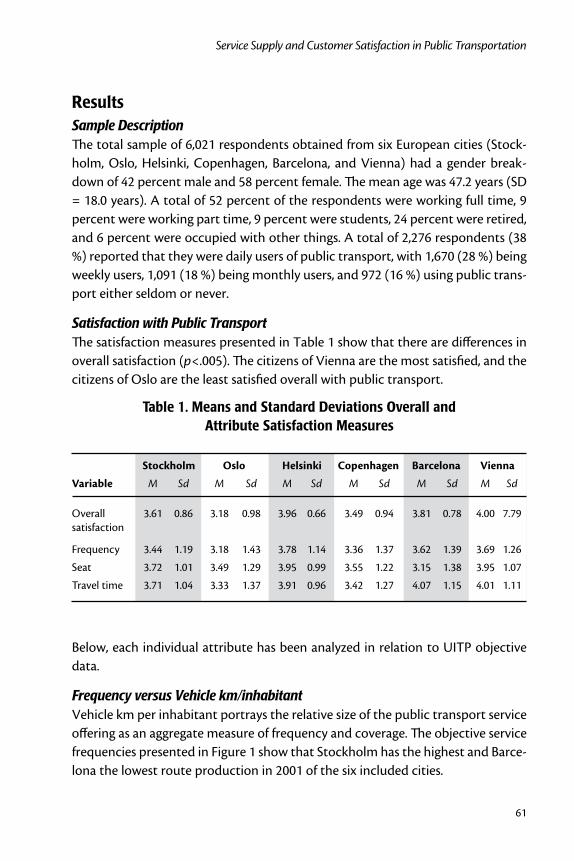
61
Service Supply and Customer Satisfaction in Public Transportation
ResultsSample DescriptionThe total sample of 6,021 respondents obtained from six European cities (Stock-holm, Oslo, Helsinki, Copenhagen, Barcelona, and Vienna) had a gender break-down of 42 percent male and 58 percent female. The mean age was 47.2 years (SD = 18.0 years). A total of 52 percent of the respondents were working full time, 9 percent were working part time, 9 percent were students, 24 percent were retired, and 6 percent were occupied with other things. A total of 2,276 respondents (38 %) reported that they were daily users of public transport, with 1,670 (28 %) being weekly users, 1,091 (18 %) being monthly users, and 972 (16 %) using public trans-port either seldom or never.
Satisfaction with Public TransportThe satisfaction measures presented in Table 1 show that there are differences in overall satisfaction (p<.005). The citizens of Vienna are the most satisfied, and the citizens of Oslo are the least satisfied overall with public transport.
Table 1. Means and Standard Deviations Overall and Attribute Satisfaction Measures
Stockholm Oslo Helsinki Copenhagen Barcelona Vienna
Variable M Sd M Sd M Sd M Sd M Sd M Sd
Overall 3.61 0.86 3.18 0.98 3.96 0.66 3.49 0.94 3.81 0.78 4.00 7.79satisfaction
Frequency 3.44 1.19 3.18 1.43 3.78 1.14 3.36 1.37 3.62 1.39 3.69 1.26
Seat 3.72 1.01 3.49 1.29 3.95 0.99 3.55 1.22 3.15 1.38 3.95 1.07
Travel time 3.71 1.04 3.33 1.37 3.91 0.96 3.42 1.27 4.07 1.15 4.01 1.11
Below, each individual attribute has been analyzed in relation to UITP objective data.
Frequency versus Vehicle km/inhabitantVehicle km per inhabitant portrays the relative size of the public transport service offering as an aggregate measure of frequency and coverage. The objective service frequencies presented in Figure 1 show that Stockholm has the highest and Barce-lona the lowest route production in 2001 of the six included cities.
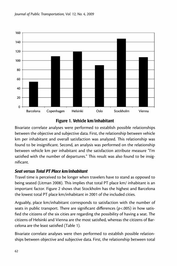
Journal of Public Transportation, Vol. 12, No. 4, 2009
62
Figure 1. Vehicle km/inhabitant
Bivariate correlate analyses were performed to establish possible relationships between the objective and subjective data. First, the relationship between vehicle km per inhabitant and overall satisfaction was analyzed. This relationship was found to be insignificant. Second, an analysis was performed on the relationship between vehicle km per inhabitant and the satisfaction attribute measure “I’m satisfied with the number of departures.” This result was also found to be insig-nificant.
Seat versus Total PT Place km/inhabitant Travel time is perceived to be longer when travelers have to stand as opposed to being seated (Litman 2008). This implies that total PT place km/ inhabitant is an important factor. Figure 2 shows that Stockholm has the highest and Barcelona the lowest total PT place km/inhabitant in 2001 of the included cities.
Arguably, place km/inhabitant corresponds to satisfaction with the number of seats in public transport. There are significant differences (p<.005) in how satis-fied the citizens of the six cities are regarding the possibility of having a seat. The citizens of Helsinki and Vienna are the most satisfied, whereas the citizens of Bar-celona are the least satisfied (Table 1).
Bivariate correlate analyses were then performed to establish possible relation-ships between objective and subjective data. First, the relationship between total
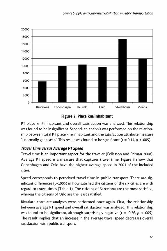
63
Service Supply and Customer Satisfaction in Public Transportation
PT place km/ inhabitant and overall satisfaction was analyzed. This relationship was found to be insignificant. Second, an analysis was performed on the relation-ship between total PT place km/inhabitant and the satisfaction attribute measure “I normally get a seat.” This result was found to be significant (r = 0.14, p < .005).
Travel Time versus Average PT SpeedTravel time is an important aspect for the traveler (Fellesson and Friman 2008). Average PT speed is a measure that captures travel time. Figure 3 show that Copenhagen and Oslo have the highest average speed in 2001 of the included cities.
Speed corresponds to perceived travel time in public transport. There are sig-nificant differences (p<.005) in how satisfied the citizens of the six cities are with regard to travel times (Table 1). The citizens of Barcelona are the most satisfied, whereas the citizens of Oslo are the least satisfied.
Bivariate correlate analyses were performed once again. First, the relationship between average PT speed and overall satisfaction was analyzed. This relationship was found to be significant, although surprisingly negative (r = -0.26, p < .005). The result implies that an increase in the average travel speed decreases overall satisfaction with public transport.
Figure 2. Place km/inhabitant
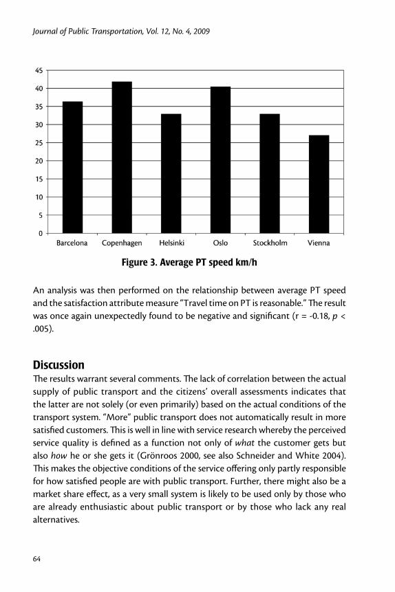
Journal of Public Transportation, Vol. 12, No. 4, 2009
64
Figure 3. Average PT speed km/h
An analysis was then performed on the relationship between average PT speed and the satisfaction attribute measure “Travel time on PT is reasonable.” The result was once again unexpectedly found to be negative and significant (r = -0.18, p < .005).
DiscussionThe results warrant several comments. The lack of correlation between the actual supply of public transport and the citizens’ overall assessments indicates that the latter are not solely (or even primarily) based on the actual conditions of the transport system. “More” public transport does not automatically result in more satisfied customers. This is well in line with service research whereby the perceived service quality is defined as a function not only of what the customer gets but also how he or she gets it (Grönroos 2000, see also Schneider and White 2004). This makes the objective conditions of the service offering only partly responsible for how satisfied people are with public transport. Further, there might also be a market share effect, as a very small system is likely to be used only by those who are already enthusiastic about public transport or by those who lack any real alternatives.
65
Service Supply and Customer Satisfaction in Public Transportation
As is indicated by the fact that respondents with either no or very limited experi-ence of the relevant public transport systems are still able to express opinions about them when asked in the survey, the level of satisfaction might be even less related to the actual transport system (Pedersen et al. 2009).
When it comes to the relationship between satisfaction with specific attributes and the objective conditions of these attributes, the results are more difficult to explain intuitively or from a theoretical point of view. There are some potential explanations for this situation, however. The lack of correlation between transport supply and frequency satisfaction might depend on the difficulties of matching supply with demand (transport may be provided but not at the time and/or loca-tion needed). Such a mismatch not being reflected in the relationship between perceived and provided seat availability could reflect the fact that the shortfall in frequency is compensated for by increased vehicle capacity. At least, the data suggest that an increase in seat availability is noted by travelers. The negative (and counterintuitive) correlation between average speed and travel time might reflect the impact of the type of travel. A long journey is likely to be perceived as time-consuming even in a fast moving vehicle. Transport systems with a high pro-portion of long distance commuter journeys might thus score lower on perceived travel time than systems primarily consisting of (comparably slow) inner city buses used primarily for short journeys as a substitute for walking.
Additional research is needed that investigates a richer set of quality attributes such as safety, staff behavior, information, and fares. Other techniques (e.g., structural equation modeling and PLS) should also be used for analyzing the relationship between traveler satisfaction measures and objective performance measures.
The study also raises the issue of what constitutes relevant measures, both of objective supply and of satisfaction. Public transport systems are inherently com-plex, and describing them using a number of standardized key indicators neces-sarily requires significant simplifications and a substantial amount of subjective interpretation (Norheim 2006, Vivier 2006). This is particularly true when data are collected on a transnational level, as is the case with the Millennium Data-base. Similarly, satisfaction is known to be difficult to measure, as it is influenced by complicated psychological and social processes. For example, a recent study revealed that customers responding to specific questions about their current journey were nonetheless taking previous experience, media coverage, and hopes of future improvements into consideration when answering (BEST 2009).
Journal of Public Transportation, Vol. 12, No. 4, 2009
66
ConclusionsDoes this mean, then, that satisfaction measures are irrelevant? Absolutely not! Satisfaction is pivotal for understanding public transport from the customer’s perspective. However, there is a problem when the subjective assessments of the users (and even the non-users) are conflated with the objective conditions of the transport system. As has been shown, a high level of satisfaction does not neces-sarily indicate an objectively “better” system and vice versa. Instead, satisfaction scores should be interpreted in their wider context, thereby enabling a further contextualization of the objective conditions as well. This is particularly important when comparisons are made between different cities: satisfaction is a relative con-cept and not a measure of absolute success in public transport.
Understanding—rather than taking for granted—the links between satisfaction and an objective service supply is a key management challenge that requires a genuine understanding of how the transport system functions, from the point of view of both the customer and production. Such a dual understanding will pro-vide an indispensible foundation for developing the public transport systems of tomorrow. Once the subjective and partly-independent nature of the satisfaction measures is acknowledged, their potential value to managers and policymakers can be realized.
Acknowledgment
This research was supported by grant #2004-02974, awarded to the Service and Market Oriented Transport Research Group (SAMOT) by the Swedish Govern-mental Agency for Innovation Systems (VINNOVA).
References
Beirão, G., and J.A. Sarsfield Cabral. 2007. Understanding attitudes towards public transport and private car: A qualitative study. Transport Policy 14: 478-489.
BEST Organizing Committee. 2001. BEST results of the 2001 survey. Oslo: BEST.
De Brentani, U. 1995. New industrial service development: Scenarios for success and failure. Journal of Business Research 32: 93-103.
67
Service Supply and Customer Satisfaction in Public Transportation
De Brentani, U. 2001. Innovative versus incremental new business services: Differ-ent keys for achieving success. Journal of Product Innovation Management 18: 169–187.
Eboli, L., and G. Mazzulla. 2007. Service quality attributes affecting customer satis-faction for bus transit. Journal of Public Transportation 10: 21-34.
Eriksson, L., M. Friman, and T. Gärling. 2009. Stated reasons for reducing work-commute by car. Transportation Research Part F: Traffic Psychology and Behaviour 11: 427-433.
Fellesson, M., and M. Friman. 2008. Perceived satisfaction with public transport services in nine European cities. The Journal of Transportation Research Forum. 47:93-103, Transit Issue Special.
Friman, M. 2004. Implementing quality improvements in public transport. Journal of Public Transportation 7: 49-65.
Friman, M., and T. Gärling. 2001. Frequency of negative critical incidents and sat-isfaction with public transport services. II. Journal of Retailing and Consumer Services 8: 105-114.
Fujii, S., and R. Kitamura. 2003. What does a one-month free bus ticket do to habitual drivers? An experimental analysis of habit and attitude change. Transportation 30: 81-95.
Grönroos, C. 2000. Service Management and Marketing: A Customer Relationship Management Approach. Chichester: Wiley.
Hauser, J.R., and D. Clausing. 1988. The house of quality. Harvard Business Review 66 (3): 63-73.
Hensher, D. A., P. Stopher, and P. Bullock. 2003. Service quality —developing a ser-vice quality index in the provision of commercial bus contracts. Transporta-tion Research Part A 37: 499-517.
Litman, T. 2008. Valuing transit service quality improvements. Journal of Public Transportation 11: 43-63.
Mackett, R. L., and M. Edwards. 1998. The impact of new public transport systems: Will the expectations be met? Transportation Research Part A: Policy and Practice 32: 231-245.
Journal of Public Transportation, Vol. 12, No. 4, 2009
68
Nagamachi, M. 1995. Kansei engineering: A new ergonomic consumer-oriented technology for product development. International Journal of Industrial Ergo-nomics 15: 3-11.
Nathanail, E. 2007. Measuring the quality of service for passengers on the Hellenic railways. Transportation Reseach Part A 42: 48-66.
Norheim, B. 2006. Kollektivtranssport i nordiske byer. Markedspotential og utfordringer framover. Norway: Urbanet analysis report no 2.
Pedersen, T., M. Friman, and P. Kristensson. (In press.) Affective forecasting: Pre-dicting and experiencing satisfaction with public transport. Journal of Applied Psychology.
Richter, J., M. Friman, and T. Gärling. 2008a. Soft transport policy measures: 1. Results of implementations. Manuscript submitted for publication.
Richter, J., M. Friman, and T. Gärling. 2008b. Soft transport policy measures: 2. Research needs. Manuscript submitted for publication.
Schneider, B., and S. White. 2004. Service Quality: Research Perspectives. Thousand Oaks: Sage.
Smith, M. J., and R. V. Clarke. 2000. Crime and public transport. In: Tonry, M. ed. Crime and Justice: A Review of Research 27. Chicago: University of Chicago Press.
Swanson, J., Ampt, L., and P. Jones. 1997. Measuring bus passenger preferences. Traffic Engineering and Control 38: 330–336.
Transportation Research Board. 2003. Transit Capacity and Quality of Service Manual. Transit Cooperative Research Program, Report 100, Washington, D.C, National Academy Press.
Tyrinopoulos, Y., and C. Antoniou. 2008. Public transit user satisfaction: Variability and policy implications. Transport Policy 15: 260-272.
Tyrinopoulos, Y., and G. Aifadopoulou. 2008. A complete methodology for the quality control of passenger services in the public transport business. Euro-pean Transport\Trasporti Europei 38: 1-16.
69
Service Supply and Customer Satisfaction in Public Transportation
Vivier, J. 2006. Mobility in Cities Database. Better Mobility for People World Wide. Analysis and Recommendations. Brussels: International Association of Public Transport.
About the Authors
Margareta Friman ([email protected]) is an associate professor, researcher, and director of the SAMOT (Service and Market Oriented Transport) research group at Karlstad University. Her research focuses on perceived service quality and customer satisfaction in public transport services. Her research has been published in the Journal of Public Transportation and the Journal of Transportation Research: Part F and the Journal of Economic Psychology.
Markus Fellesson, Ph.D. ([email protected]) is a researcher in the SAMOT research group at Karlstad University. His research focuses on various aspects of customer-orientation as a managerial practice. He is co-author of Marketing Discourse—A Critical Perspective, published by Routledge. His research also has been published in the Scandinavian Journal of Management, the Journal of the Transport Research Forum, and Revista ADM.MADE.
Journal of Public Transportation, Vol. 12, No. 4, 2009
70
71
Transit “Pass-Through” Lanes at Freeway Interchanges
Transit “Pass-Through” Lanes at Freeway Interchanges: A Life-Cycle
Evaluation MethodologyMichael Mandelzys and Bruce Hellinga
University of Waterloo
Abstract
Transit “pass-through” lanes provide transit vehicle priority at freeway interchanges. “Pass-through” lanes allow a transit vehicle to exit the freeway at an interchange, cross straight through the intersecting arterial road, and re-enter the freeway. This treatment allows transit vehicles to bypass congestion on the mainline between the beginning of the off-ramp and the end of the on-ramp.
This paper outlines a methodology to evaluate if transit “pass-through” lanes are economically justified at a given interchange and provides a method for prioritizing candidate locations. The methodology provides an objective and consistent deci-sion making method, reduces the effort required for practitioners to assess the need for “pass-through” treatment at a given interchange, and helps ensure that limited resources are directed towards interchanges that are expected to experience the greatest benefit per dollar spent.
The proposed methodology is based on an analytical approach that compares the value of travel time savings (for passengers and transit vehicles) with the construction and maintenance costs of the transit “pass-through” lane treatment.
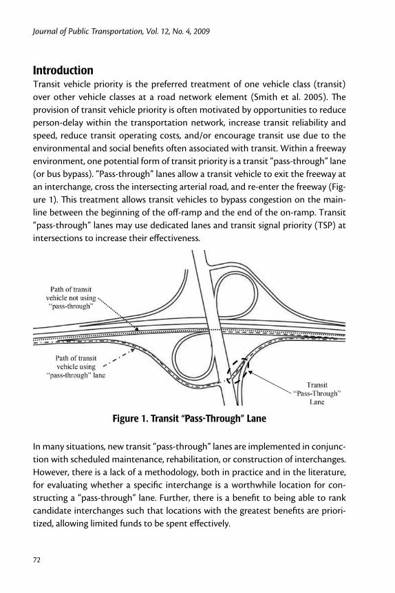
Journal of Public Transportation, Vol. 12, No. 4, 2009
72
IntroductionTransit vehicle priority is the preferred treatment of one vehicle class (transit) over other vehicle classes at a road network element (Smith et al. 2005). The provision of transit vehicle priority is often motivated by opportunities to reduce person-delay within the transportation network, increase transit reliability and speed, reduce transit operating costs, and/or encourage transit use due to the environmental and social benefits often associated with transit. Within a freeway environment, one potential form of transit priority is a transit “pass-through” lane (or bus bypass). “Pass-through” lanes allow a transit vehicle to exit the freeway at an interchange, cross the intersecting arterial road, and re-enter the freeway (Fig-ure 1). This treatment allows transit vehicles to bypass congestion on the main-line between the beginning of the off-ramp and the end of the on-ramp. Transit “pass-through” lanes may use dedicated lanes and transit signal priority (TSP) at intersections to increase their effectiveness.
Figure 1. Transit “Pass-Through” Lane
In many situations, new transit “pass-through” lanes are implemented in conjunc-tion with scheduled maintenance, rehabilitation, or construction of interchanges. However, there is a lack of a methodology, both in practice and in the literature, for evaluating whether a specific interchange is a worthwhile location for con-structing a “pass-through” lane. Further, there is a benefit to being able to rank candidate interchanges such that locations with the greatest benefits are priori-tized, allowing limited funds to be spent effectively.
73
Transit “Pass-Through” Lanes at Freeway Interchanges
The evaluation and ranking of priority treatments can be done on the basis of relative benefits and costs associated with the treatments. In practice, detailed benefit/cost ranking tends to be cumbersome and time-consuming to conduct; therefore, it can be beneficial to embed the benefit/cost analysis within a simpli-fied warrant procedure.
This paper outlines a warrant methodology that can be used to aid in determin-ing whether or not construction of a transit “pass-through” lane at a given inter-change is justified and provides a method for prioritizing candidate locations. The warrant methodology provides an objective and consistent decision making method, reduces the effort required for practitioners to assess the effectiveness of a “pass-through” treatment at a given interchange, and helps ensure that limited resources are directed towards interchanges that are expected to experience the greatest benefit per dollar spent.
The proposed methodology is based on an analytical approach to estimate expected daily travel time savings (for passengers and for transit vehicles) associ-ated with providing transit “pass-through” lanes. The expected benefits of the treatment are derived by converting travel time savings into a dollar value. Costs of the treatment are estimated on the basis of annualized construction cost and estimated annual maintenance costs. The output of the methodology is a benefit/cost ratio (BCR).
MethodologyTransit priority treatments are often evaluated via analytical or microsimulation methods. To provide the repeatability and ease of use typically associated with a warrant methodology, the procedure outlined in this paper is based on analytical methods.
The ultimate output of the warrant methodology is a BCR. If the BCR exceeds a certain threshold (typically 1.0), the proposed transit “pass-through” is evaluated as economically warranted. The BCR is also useful for comparing potential inter-changes (FHWA 2003) and prioritizing those interchanges that will receive the greatest benefit per dollar spent.
The warrant methodology analyzes typical weekday conditions from 6:00 a.m. until 9:00 p.m., broken up into 15-minute periods to capture temporal variations in traffic conditions and bus frequencies. Data requirements to complete the war-rant methodology consist of:
Journal of Public Transportation, Vol. 12, No. 4, 2009
74
Freeway segment length (km)•
Bypass segment length (km)•
Freeway speed profile (km/hr, per 15-minute period)•
Off-ramp volume for lane group used for bypass •(veh, per 15-minute period)
Intersection configuration•
Heavy vehicle percentage for lane group used for bypass (%)•
Traffic signal timing plan•
Transit signal priority parameters, if applicable•
Transit vehicle schedule•
Transit vehicle loadings (passengers/vehicle)•
Capital (construction) cost of bypass infrastructure ($)•
Service life of bypass infrastructure (years)•
Annual maintenance cost of bypass infrastructure ($)•
Benefit EstimationThe benefit estimation portion of the warrant methodology involves estimating the travel time savings for transit vehicle passengers and the travel time savings for transit vehicles. These two values are used to quantify benefits such as reduced travel time for users, reduced vehicle requirements for transit agencies, reduced transit vehicle fuel consumption, and potential modal shifts from personal vehi-cles to transit among commuters.
The benefit estimation procedure is summarized in Figure 2 and consists of the following steps.
Benefit Calculation Step 1: Construct Freeway Travel Time Profile
Travel time for a bus along the mainline of the freeway (i.e., assuming the proposed transit “pass-through” lane is not used) is estimated for each 15-minute time period throughout the day. Travel time is calculated for each period based on freeway speeds (typically measured using loop detectors or other dedicated traffic sensors) in the vicinity of the interchange and the distance along the mainline that could be skipped by using the bypass (Equation 1).
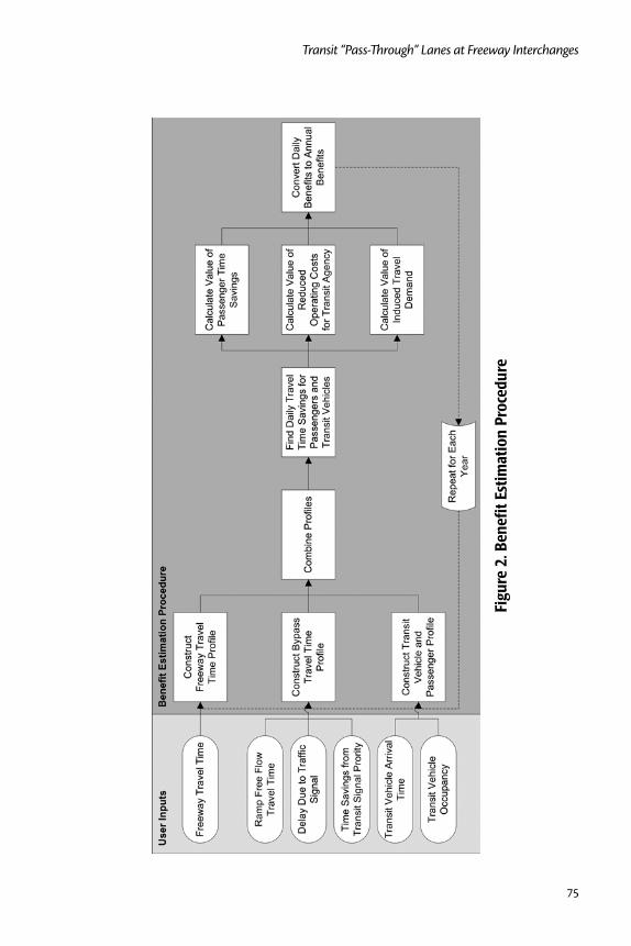
75
Transit “Pass-Through” Lanes at Freeway Interchanges
Figu
re 2
. Ben
efit E
stim
atio
n Pr
oced
ure
Journal of Public Transportation, Vol. 12, No. 4, 2009
76
(1)
Where TTFreeway,i is the travel time on the freeway in period i, in seconds
DFreeway is the distance along the freeway which the transit vehicle would avoid if it used the bypass, in km
VFreeway,i is the speed on the mainline freeway in period i, in km/hr
The resulting output of this step is a freeway travel time profile over the course of a typical weekday. It is also possible to construct the freeway travel time profile directly using observed/archived travel time data for the freeway in the vicinity of the interchange.
Benefit Calculation Step 2: Construct Bypass Travel Time Profile
Travel time for a bus using the transit “pass-through” lane is based on free-flow travel time along the bypass route, plus an additional delay due to the traffic signal at the arterial road crossing, minus some time savings from TSP if it is provided. Conceptually, the travel time for the bypass is calculated during each period as follows (Equation 2):
TTBypass,i = TTBypassFreeflow + TTSignal,i - TTTSP,i (2)
Where TTBypass,i is the travel time on the bypass in period i, in seconds
TTBypassFreeflow is the travel time on the bypass assuming free-flow conditions, in seconds
TTSignal,i is the additional travel time added by the traffic signal at the crossing arterial road during period i, in seconds
TTTSP,i is the travel time savings attributable to transit signal priority at the traffic signal at the crossing arterial road during period i, in seconds
The travel time for the bypass under free-flow conditions is an idealized time that assumes that the route could be completed without the need to stop or slow
77
Transit “Pass-Through” Lanes at Freeway Interchanges
due to the traffic signal or queues at the traffic signal. This free-flow travel time is, therefore, limited by the geometry and speed limit of the bypass route. Calculation of travel time for the bypass under free-flow conditions is indicated in Equation 3. Since this value is independent of traffic volumes and signal operation, it is con-stant during all time periods.
(3)
Where DBypass is the distance travelled on the bypass, in km
VBypassFreeflow is the average free-flow speed on the bypass, in km/hr
Having to cross an arterial road at a traffic signal adds travel time to the bypass. The amount of additional travel time is a function of traffic volumes, signal timings, driver behavior, and intersection configuration and will therefore vary throughout the day. The additional delay due to the traffic signal during each period is estimated by following the methodology outlined in Chapter 16 of the Highway Capacity Manual 2000 (Transportation Research Board 2000), as outlined in Equation 4.
TTSignal,i = d1 + d2 + d3 (4)
Where d1 is the uniform control delay based uniform arrivals, in seconds
d2 is the incremental delay due to random arrivals and oversaturation queues, in seconds
d3 is the initial queue delay, in seconds
The delay due to the traffic signal can be partially mitigated through the provi-sion of transit signal priority. To quantify the expected delay reduction due to transit signal priority, a simplified analytical model has been used (Lin 2002). The model presents expected delay reduction as a function of the “aggressiveness” of the transit signal priority parameters, i.e., the maximum green extension and red truncation permitted (Equation 5).

Journal of Public Transportation, Vol. 12, No. 4, 2009
78
(5)
Where C is the cycle length, in seconds
R is the length of red phase for the bus approach, in seconds
Rmin is the minimum permissible red phase for the bus approach, in seconds
is the maximum permissible green extension for the bus approach, in seconds
Note that the total signal delay (TTSignal,i ) acts as an upper bound on the travel time savings due to TSP (TTTSP,i ).
The resulting output of this step is a bypass travel time profile over the course of a typical weekday.
Benefit Calculation Step 3: Construct Transit Vehicle and Passenger Profile
A daily profile of transit use (in terms of both number of passengers and number of vehicles) must be known to evaluate the effectiveness of a proposed bypass. The profile can be created based on a known or planned transit schedule and based on a known or assumed bus occupancy level. The profile must identify the number of buses and passengers expected during each period
Benefit Calculation Step 4: Combine Profiles and Find Daily Travel Time Savings
The daily travel time savings, in terms of passenger hours and transit vehicle hours saved, can be found. by combining the profiles created in steps 1 to 3.
The transit “pass-through” lane provides a benefit only during periods in which a transit vehicle’s travel time using the bypass is less than its travel time using the freeway. During periods when this is not the case, it is likely that the transit vehicle will simply stay on the freeway, and the bypass will not be used. As well, regardless of the difference in travel times between the freeway and the bypass, travel time savings can be accrued only during periods in which transit vehicles are scheduled to arrive. Therefore, travel time savings exist only during specific periods of the day. Travel time savings during each of these periods can be calculated as the difference between travel time on the bypass and travel time on the freeway multiplied by
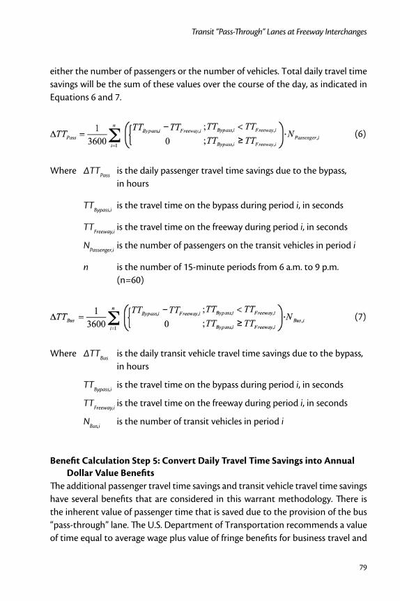
79
Transit “Pass-Through” Lanes at Freeway Interchanges
either the number of passengers or the number of vehicles. Total daily travel time savings will be the sum of these values over the course of the day, as indicated in Equations 6 and 7.
(6)
Where ΔTTPass is the daily passenger travel time savings due to the bypass, in hours
TTBypass,i is the travel time on the bypass during period i, in seconds
TTFreeway,i is the travel time on the freeway during period i, in seconds
NPassenger,i is the number of passengers on the transit vehicles in period i
n is the number of 15-minute periods from 6 a.m. to 9 p.m. (n=60)
(7)
Where ΔTTBus is the daily transit vehicle travel time savings due to the bypass, in hours
TTBypass,i is the travel time on the bypass during period i, in seconds
TTFreeway,i is the travel time on the freeway during period i, in seconds
NBus,i is the number of transit vehicles in period i
Benefit Calculation Step 5: Convert Daily Travel Time Savings into Annual Dollar Value Benefits
The additional passenger travel time savings and transit vehicle travel time savings have several benefits that are considered in this warrant methodology. There is the inherent value of passenger time that is saved due to the provision of the bus “pass-through” lane. The U.S. Department of Transportation recommends a value of time equal to average wage plus value of fringe benefits for business travel and
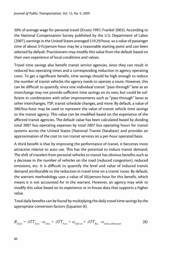
Journal of Public Transportation, Vol. 12, No. 4, 2009
80
50% of average wage for personal travel (Kruesi 1997, Frankel 2003). According to the National Compensation Survey published by the U.S. Department of Labor (2007), earnings in the United States averaged $19.29/hour, so a value of passenger time of about $15/person-hour may be a reasonable starting point and can been selected by default. Practitioners may modify this value from the default based on their own experience of local conditions and values.
Travel time savings also benefit transit service agencies, since they can result in reduced bus operating times and a corresponding reduction in agency operating costs. To get a significant benefit, time savings should be high enough to reduce the number of transit vehicles the agency needs to operate a route. However, this can be difficult to quantify, since one individual transit “pass-through” lane at an interchange may not provide sufficient time savings on its own, but could be suf-ficient in combination with other improvements such as “pass-through” lanes at other interchanges, TSP, transit schedule changes, and more. By default, a value of $80/bus-hour may be used to represent the value of transit vehicle time savings to the transit agency. This value can be modified based on the experience of the affected transit agencies. The default value has been calculated based by dividing total 2007 bus operating expenses by total 2007 bus operating hours for transit systems across the United States (National Transit Database) and provides an approximation of the cost to run transit services on a per-hour operated basis.
A third benefit is that by improving the performance of transit, it becomes more attractive relative to auto use. This has the potential to induce transit demand. The shift of travelers from personal vehicles to transit has obvious benefits such as a decrease in the number of vehicles on the road (reduced congestion), reduced emissions, etc. It is difficult to quantify the level and value of induced transit demand attributable to the reduction in travel time on a transit route. By default, the warrant methodology uses a value of $0/person-hour for this benefit, which means it is not accounted for in the warrant. However, an agency may wish to modify this value based on its experience or in-house data that supports a higher value.
Total daily benefits can be found by multiplying the daily travel time savings by the appropriate conversion factors (Equation 8):
BDaily = ΔTTPass · Time + ΔTTPass + OpCost + ΔTTBus · InducedDemand (8)
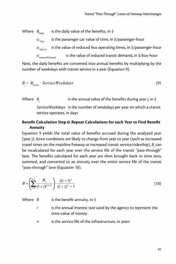
81
Transit “Pass-Through” Lanes at Freeway Interchanges
Where BDaily is the daily value of the benefits, in $
Time is the passenger car value of time, in $/passenger-hour
OpCost is the value of reduced bus operating times, in $/passenger-hour
InducedDemand is the value of induced transit demand, in $/bus-hour
Next, the daily benefits are converted into annual benefits by multiplying by the number of weekdays with transit service in a year (Equation 9).
Bj = BDaily · ServiceWeekdays (9)
Where Bj is the annual value of the benefits during year j, in $
ServiceWeekdays is the number of weekdays per year on which a transit service operates, in days
Benefit Calculation Step 6: Repeat Calculations for each Year to Find Benefit Annuity
Equation 9 yields the total value of benefits accrued during the analyzed year (year j). Since conditions are likely to change from year to year (such as increased travel times on the mainline freeway or increased transit service/ridership), Bj can be recalculated for each year over the service life of the transit “pass-through” lane. The benefits calculated for each year are then brought back to time zero, summed, and converted to an annuity over the entire service life of the transit “pass-through” lane (Equation 10).
(10)
Where B is the benefit annuity, in $
i is the annual interest rate used by the agency to represent the time-value of money
n is the service life of the infrastructure, in years
Journal of Public Transportation, Vol. 12, No. 4, 2009
82
Evidently, this step significantly increases the data and workload requirements of the warrant procedure, since the calculation of Bj for each year requires re-computing all the previous steps for each year.
In many situations, the methodology can be simplified by assuming that condi-tions remain constant over the service life of the improvement. Although this assumption is not strictly true, it greatly simplifies the calculation of the benefit annuity, B, such that it is simply equal to the annual benefits calculated for year 0 (B0). The assumption will frequently result in a conservative bias in the warrant methodology since, in most cases, conditions in the future tend to favor improve-ments more so than conditions today. This is because congestion is frequently projected to increase and, correspondingly, traffic speeds on the freeway are being reduced as time goes on. Further, transit service/usage is typically expected to remain constant or increase at locations where transit improvements are being considered. Both these factors have the potential to lead to even greater benefits from a transit “pass-through” lane in future years. By not accounting for these factors, we are frequently providing a conservative benefit of the true estimates. Therefore, when using this simplifying assumption, if a “pass-through” is war-ranted using the current methodology, then it would likely also be warranted had speed profile changes over time been taken into account.
In general, it is recommended that the warrant be completed first with the simplifying assumption that conditions remain constant. Unless freeway speeds are expected to increase in the future, or transit use is expected to decrease, an interchange that meets the warrant requirements with this simplifying assump-tion should also meet the warrant requirements if changes in conditions had been accounted for. In situations where significant changes in travel time or transit profiles are expected over the service life of the transit “pass-through” lane, it may be worthwhile to discard the simplifying assumption and calculate the benefits for each year as outlined in this step to determine if the results of the warrant are significantly affected.
Cost EstimationCosts of a transit “pass-through” lane treatment are estimated on the basis of con-struction and maintenance costs. The cost estimation procedure is summarized in Figure 3 and consists of the following steps.
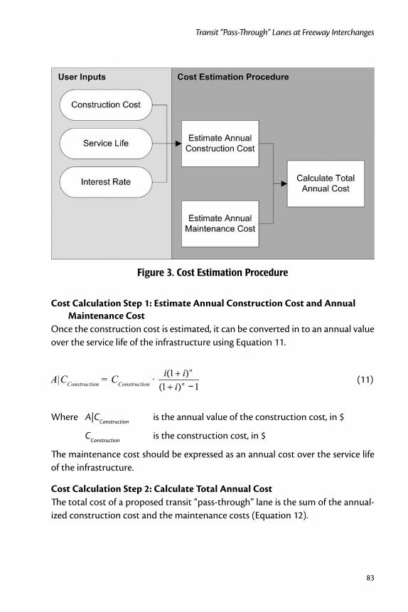
83
Transit “Pass-Through” Lanes at Freeway Interchanges
Figure 3. Cost Estimation Procedure
Cost Calculation Step 1: Estimate Annual Construction Cost and Annual Maintenance Cost
Once the construction cost is estimated, it can be converted in to an annual value over the service life of the infrastructure using Equation 11.
A|CConstruction = CConstruction · (11)
Where A|CConstruction is the annual value of the construction cost, in $
CConstruction is the construction cost, in $
The maintenance cost should be expressed as an annual cost over the service life of the infrastructure.
Cost Calculation Step 2: Calculate Total Annual CostThe total cost of a proposed transit “pass-through” lane is the sum of the annual-ized construction cost and the maintenance costs (Equation 12).
Journal of Public Transportation, Vol. 12, No. 4, 2009
84
C = A|CConstruction + A|CMaintenance (12)
Where C is the annual value of the costs, in $
A|CMaintenance is the annual maintenance costs, in $
The full warrant methodology has been implemented in an automated spread-sheet format to ease its application.
InterpretationThe ultimate output of the warrant is a benefit/cost ratio (BCR). The transit “pass-through” lane meets the minimum requirements of the warrant when the BCR exceeds a certain threshold. Typically, this threshold will be 1.0 (benefits exceed costs); however, individual agencies should have some flexibility in the threshold for meeting the warrant. This flexibility recognizes that the warrant represents a simplified BCR and that its results are subject to the assumptions and limitations as outlined previously.
In addition to evaluating whether a transit “pass-through” lane is warranted at a given location, the warrant methodology can be used to easily compare multiple potential locations. Locations that meet the minimum requirements of the war-rant can be ranked from highest BCR to lowest BCR, which allows those loca-tions that are expected to experience the greatest benefit per dollar spent to be prioritized over locations that also meet the minimum warrant requirements but provide relatively lower benefits for the investment.
Assumptions and LimitationsWhen developing a warrant methodology, there is a need to find an appropriate balance between complexity and accuracy. The time and data requirements to complete the warrant methodology should not act as an impediment to its use, while still ensuring that the output of the warrant is of sufficient accuracy to allow the warrant be used as the decision making tool it is intended to be.
To achieve this balance, the proposed warrant methodology relies on several assumptions to simplify application and minimize excessive data requirements. The following key assumptions are made in this warrant methodology:
HCM 2000 signalized delay calculations are applicable. Since this warrant •methodology uses the HCM 2000 signalized delay equations to estimate the

85
Transit “Pass-Through” Lanes at Freeway Interchanges
delay experienced by the transit vehicle when passing through the signal-ized intersection, the assumptions included in the HCM 2000 method are inherently part of this warrant methodology.
Simplified TSP delay reduction equation is applicable. This methodology •uses a simplified analytical equation to estimate expected delay reductions from transit signal priority. This equation makes several simplifying assump-tions, including that the bus is detected and reacted to instantly by the TSP system and that buses have sufficient headways such that TSP system recovery time is not a factor (Lin 2002).
In addition to the assumptions discussed above, there are also several factors which are not considered in the warrant in order to maintain simplicity. These factors include the following and are discussed in greater detail by Mandelzys and Hellinga (2009):
Disbenefit to cross-street traffic•
Improvements in service reliability•
Potential for transit stops at interchanges•
ApplicationThe application of the warrant methodology is illustrated for a freeway inter-change (Highway 401 Eastbound/Avenue Road) in southern Ontario. This inter-change had a transit “pass-through” lane constructed in 2007; however, the “pass-through” lane is not yet in use.
Highway 401 is a major freeway within the city of Toronto. The eastbound direc-tion of Highway 401 operates with an express-collector configuration at Avenue Road, with the Avenue Road exit available only from the collector lanes. A full-day freeway speed profile was not available at this location; therefore, the freeway speed profile was estimated based on data collected in a 2006 travel time study for the Ontario Ministry of Transportation (MTO). The travel time study used probe vehicles and focused on peak AM, midday, and PM periods. Since there was a limited sampling frequency, travel times were interpolated during peak periods, and the freeway was assumed to be free-flowing at all other times. As well, to simplify calculations and because there was no information available to estimate future freeway travel time profiles or transit schedules/ridership, we have made the simplifying assumption that conditions remain constant in future years. The data sources used are summarized in Table 1.
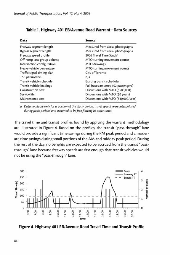
Journal of Public Transportation, Vol. 12, No. 4, 2009
86
Table 1. Highway 401 EB/Avenue Road Warrant—Data Sources
Data Source
Freeway segment length Measured from aerial photographsBypass segment length Measured from aerial photographsFreeway speed profile 2006 Travel Time Studya
Off-ramp lane group volume MTO turning movement countsIntersection configuration MTO drawingsHeavy vehicle percentage MTO turning movement countsTraffic signal timing plan City of TorontoTSP parameters n/aTransit vehicle schedule Existing transit schedulesTransit vehicle loadings Full buses assumed (52 passengers)Construction cost Discussions with MTO ($500,000)Service life Discussions with MTO (30 years)Maintenance cost Discussions with MTO ($10,000/year)
a Data available only for a portion of the study period; travel speeds were interpolated during peak periods and assumed to be free-flowing at other times.
The travel time and transit profiles found by applying the warrant methodology are illustrated in Figure 4. Based on the profiles, the transit “pass-through” lane would provide a significant time savings during the PM peak period and a moder-ate time savings during small portions of the AM and midday peak period. During the rest of the day, no benefits are expected to be accrued from the transit “pass-through” lane because freeway speeds are fast enough that transit vehicles would not be using the “pass-through” lane.
Figure 4. Highway 401 EB/Avenue Road Travel Time and Transit Profile
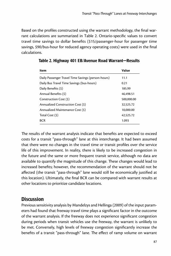
87
Transit “Pass-Through” Lanes at Freeway Interchanges
Based on the profiles constructed using the warrant methodology, the final war-rant calculations are summarized in Table 2. Ontario-specific values to convert travel time savings to dollar benefits ($15/passenger-hour for passenger time savings, $90/bus-hour for reduced agency operating costs) were used in the final calculations.
Table 2. Highway 401 EB/Avenue Road Warrant—Results
Item Value
Daily Passenger Travel Time Savings (person-hours) 11.1
Daily Bus Travel Time Savings (bus-hours) 0.21
Daily Benefits ($) 185.99
Annual Benefits ($) 46,498.51
Construction Cost ($) 500,000.00
Annualized Construction Cost ($) 32,525.72
Annualized Maintenance Cost ($) 10,000.00
Total Cost ($) 42,525.72
BCR 1.093
The results of the warrant analysis indicate that benefits are expected to exceed costs for a transit “pass-through” lane at this interchange. It had been assumed that there were no changes in the travel time or transit profiles over the service life of this improvement. In reality, there is likely to be increased congestion in the future and the same or more frequent transit service, although no data are available to quantify the magnitude of this change. These changes would lead to increased benefits; however, the recommendation of the warrant should not be affected (the transit “pass-through” lane would still be economically justified at this location). Ultimately, the final BCR can be compared with warrant results at other locations to prioritize candidate locations.
DiscussionPrevious sensitivity analysis by Mandelzys and Hellinga (2009) of the input param-eters had found that freeway travel time plays a significant factor in the outcome of the warrant analysis. If the freeway does not experience significant congestion during periods when transit vehicles use the freeway, the warrant is unlikely to be met. Conversely, high levels of freeway congestion significantly increase the benefits of a transit “pass-through” lane. The effect of ramp volume on warrant
Journal of Public Transportation, Vol. 12, No. 4, 2009
88
outcome was found to be minimal, except when ramp volumes approached or exceeded capacity. The transit schedule was found to be important, since benefits can be accrued only during time periods when transit vehicles actually travel through the study area. Finally, the choice of multiplication factors (to convert time savings to benefits) was found to affect the BCR in a linear manner with the rate of change being proportional to the amount of time savings expected
In consideration of these findings, Mandelzys and Hellinga (2009) recommended that full data collection is unlikely to be needed for the entire 6 a.m. to 9 p.m. period. Instead, with minimal impact on the output of the warrant methodology, data collection could be limited to periods containing any one of:
notable freeway congestion•
high ramp volumes•
notable transit volumes•
Under most circumstances, the time periods of the above three cases can be expected to roughly coincide.
ConclusionsOne form of providing transit vehicle priority within a freeway environment is to create transit “pass-through” lanes at interchanges. “Pass-through” lanes allow a vehicle to exit the mainline of the freeway at an off-ramp, cross straight across the intersecting arterial road, and re-enter the freeway via the on-ramp. When the mainline of the freeway is heavily congested, this allows the transit vehicle to bypass a significant portion of the freeway.
These treatments frequently are implemented on an ad-hoc basis, and there is a lack of a consistent methodology to determine if the benefits of implementing a transit “pass-through” lane treatment at a given location justify the associated costs. This paper outlines a warrant methodology that can be used to test individ-ual candidate interchanges and to rank the locations such that interchanges with the greatest relative benefits are prioritized over interchanges with lower relative benefits. The output of the warrant methodology is a benefit/cost ratio.
It was found that freeway speeds have a significant influence on the results of the warrant analysis. If freeway speeds are generally high throughout the day, the warrant is unlikely to be met. Lane group volumes at the signalized intersection of the off-ramp have a smaller effect on the outcome of the warrant, unless volumes
89
Transit “Pass-Through” Lanes at Freeway Interchanges
approach or exceed capacity. The transit schedule is also important, as travel time benefits are accrued only during periods in which transit vehicles pass through the interchange. Therefore, the key periods for the warrant to analyze should include times when (a) there is significant freeway congestion, (b) there are high-volumes on the transit “pass-through” lane group, or (c) there are notable transit volumes.
This methodology forms a good basis for analyzing potential interchanges for transit “pass-through” lanes in the future. The methodology is beneficial as it provides an objective and consistent decision making method, reduces the effort required to assess the need for “pass-through” treatment at a given interchange, and ensures that limited resources are directed towards interchanges that are expected to experience the greatest benefit per dollar spent.
Recommendations
A transit “pass-through” lane treatment would seem to interact well with bus-on-shoulder operations, since it can eliminate the need to exit the shoulder and cross over mixed traffic at the interchanges. The precise benefits may vary by applica-tion, but they are not currently accounted for in the methodology. Accounting for the benefit of combining transit “pass-through” lanes with bus-on-shoulder operations may be an area for future research.
This methodology is limited to estimating effects at a single interchange. Ulti-mately, it would be beneficial for the methodology to include a mechanism for considering an entire corridor of interchanges, since this would allow interactions between interchanges and the cumulative effects of time savings to be investigated more thoroughly. The analysis has been limited to single interchanges at this time to reflect the limited scale of implementation being considered by many transit agencies. It is our understanding that transit “pass-through” lane treatments often are considered for only a few interchanges and/or in conjunction with already scheduled interchange construction/maintenance/rehabilitation. A corridor-wide warrant methodology is a potential area for future research.
This methodology could be considered for inclusion in the Highway Capacity Manual or the Transit Capacity and Quality of Service Manual to disseminate the techniques to practitioners.
Journal of Public Transportation, Vol. 12, No. 4, 2009
90
Acknowledgments
The authors would like to thank the Ontario Ministry of Transportation for its technical support and feedback, as well as for funding this research. Special thanks is given to Ms. Nancy Adriano for her time and input in completing this research. The findings described in this paper are those of the authors and should not be interpreted to represent Ontario Ministry of Transportation policy.
References
FHWA. 2003. Economic Analysis Primer. Publication FHWA-IF-03-032. Washing-ton, D.C.: Office of Asset Management, FHWA, U.S. Department of Transpor-tation.
Frankel, E. H. 2003. Revised Departmental Guidance: Valuation of Travel Time in Economic Analysis. Office of the Secretary of Transportation, U.S. Department of Transportation.
Kruesi, F. E. 1997. Departmental Guidance for the Valuation of Travel Time in Eco-nomic Analysis. Office of the Secretary of Transportation, U.S. Department of Transportation.
Lin, W-H. 2002. Quantifying delay reduction to buses with signal priority treatment in mixed-mode operation. Transportation Research Record 1811: 100-106.
Mandelzys, M., and B. Hellinga. 2009. Warrant methodology for evaluating and ranking transit “pass-through” lanes at freeway interchanges. Paper presented at the annual meeting of the Transportation Research Board, January 11-15, Washington D.C.
National Transit Database. National Transit Database—Data—TS2.1 - Service Data and Operating Expenses Time-Series by Mode. http://www.ntdprogram.gov/ntdprogram/data.htm.
Smith, H. R., B. Hemily, and M. Ivanovic. 2005. Transit Signal Priority: A Planning and Implentation Handbook. ITS America.
Transportation Research Board. 2000. Highway Capacity Manual 2000. Washing-ton, D.C.: Transportation Research Board.
91
Transit “Pass-Through” Lanes at Freeway Interchanges
U.S. Department of Labor, U.S. Bureau of Labor Statistics. 2007. National Compen-sation Survey: Occupational Wages in the United States, June 2006. Summary 07-03. Washington, D.C.: U.S. Department of Labor.
About the Authors
Michael Mandelzys ([email protected]) received an undergraduate degree in Civil Engineering from the University of Waterloo, followed by several years of work experience in transportation planning and design at LEA Consulting, a transportation consultant in Toronto. In 2007, he returned to the University of Waterloo as a graduate student and currently is pursuing an MASc with a research focus in transit.
Dr. Bruce Hellinga ([email protected]) received BASc and MASc degrees in Civil Engineering from the University of Waterloo in 1989 and 1990 and a PhD in Civil Engineering-Transportation from Queen’s University in Kingston, Ontario, in 1994. Currently, he is an Associate Professor in the Department of Civil and Environ-mental Engineering at the University of Waterloo. He has authored or coauthored more than 90 technical papers and reports reflecting his research interests in traffic engineering and control, traffic and transit modeling, safety and ITS, with financial support from a number of public and private sector agencies including the Natural Sciences and Engineering Research Council of Canada and federal, provincial, and municipal transportation agencies.

A Case Study of Job Access and Reverse Commute Programs
93
A Case Study of Job Access and Reverse Commute Programs in the
Chicago, Kansas City, and San Francisco Metropolitan Regions
J.S. Onésimo Sandoval, St. Louis University Eric Petersen, Cambridge Systematics
Kim L. Hunt, O-H Community Partners, Ltd.
Abstract
The 1996 federal welfare-to-work legislation generated significant debate regarding what role public transportation should play in facilitating lower welfare rates. Given this debate, transportation has been called the “to” component of welfare-to-work. In this paper, we present findings from three case studies that examine job accessibil-ity and reverse commute transportation programs in the Chicago, Kansas City, and San Francisco metropolitan regions. We explored how institutional and/or grassroots support prevented or fostered the innovation and implementation of non-traditional Access-to-Jobs and Reverse Commute (JARC) programs. Our findings suggest that institutional support and grassroots support are necessary ingredients for the imple-mentation of innovative transportation programs for low-income families.
IntroductionIn 1996, Congress passed a sweeping welfare reform law called the Personal Responsibility and Work Opportunity Reconciliation Act (PRWORA), which replaced the existing welfare entitlement program. One aspect of PRWORA that
Journal of Public Transportation, Vol. 12, No. 4, 2009
94
has impacted urban and rural transportation services was the requirement that welfare recipients find full-time employment. Congress recognized that the poor faced a major spatial mismatch in terms of where they lived (typically, central cit-ies) and where new employment opportunities were located (generally, the outer suburbs) (Kasarda 1988; Gomez Ibanez 1984; Sanchez et al. 2003). The spatial mismatch makes commuting to suburban job centers difficult (to say nothing of finding a new job in the first place), but particularly challenging for workers (or potential workers) who do not have access to a car. One of the major obstacles welfare mothers faced as they tried to find work was an insufficient transportation infrastructure to overcome the spatial mismatch (Blumenberg 2002; Blumenberg and Manville 2004; Cervero 2004; Ortoleva and Brenman 2004; Sanchez et al. 2004). In response to inadequate transit access and service, several policy pro-grams were designed to provide and fund reliable transportation for low-income families.1 The underlying goal for all these programs was to provide flexible trans-portation to increase economic opportunity. The primary funds for transporta-tion services for Temporary Assistance for Needy Families (TANF) recipients came from TANF (user-side subsidies), Welfare-to-Work Grants (Department of Labor), and Bridges-to-Work (Blumenberg 2002; Government Accounting Office 1998). However, the U.S. Department of Transportation (DOT) proposed the creation of a much larger $600 million Access-to-Jobs program to be administered by the Federal Transit Administration (FTA) (Government Accounting Office 1998). The Transportation Equity Act for the 21st Century (TEA-21) established the Access-to-Jobs and Reverse Commute (JARC) program in 1998 and authorized up to $750 million over five years to implement the program.
One important aspect of the JARC program was that TEA-21 limited funding of Access-to-Jobs programs to 50 percent of each grantee’s project, unlike the 80 percent match generally available for highway projects and New Start transit proj-ects (Government Accounting Office 1998). The policy incentive was designed to encourage local, regional, and state agencies to collaborate with each other as they designed transportation policies. Another important aspect of the policy was that JARC was designed to be a competitive granting process. The rationale behind this aspect of the program was to fund the most innovative and effective transporta-tion programs for low-income families. Policy makers conceded that “existing public transportation systems cannot always bridge the gap between where the poor live and where jobs are located” (Government Accounting Office 1998). The policy incentive strongly encouraged traditional transportation agencies to work with local grassroots organizations in an effort to explore all non-traditional trans-
A Case Study of Job Access and Reverse Commute Programs
95
portation alternatives to the fixed route or existing mass transit systems (Govern-ment Accounting Office 1998).
There is no question that the JARC programs distributed a large sum of transporta-tion funding targeted towards low-income populations. However, it is not clear if this funding was effective in allowing individuals to move into the workforce, par-ticularly since the evaluations conducted by the Government Accounting Office (GAO) focused more on the process of awarding JARC funds rather than program outcomes. Moreover, the lasting impact of the JARC funds is not clear. While there was hope that JARC funds would serve as seed money to get deserving proj-ects off the ground, program implementers seemed to accept that many projects were experimental and would not be made permanent. This raises a legitimate point about the long-term sustainability of JARC programs.
The critics of JARC were right to ask whether JARC programs were merely a cosmetic policy remedy or if the programs truly were designed to eliminate the deep structural inequalities built into the existing mass transportation systems. If the primary goal was the elimination or at least reduction of structural inequal-ity, then phasing out federal funding sent the wrong message, unless one truly believed that, with one major push, people would leave and remain off of welfare. In reality, few metropolitan regions have the fiscal resources to maintain these programs without additional federal support. Pittsburgh is only one of many cases where budgetary crises have led to the proposed elimination of JARC programs (Curry 2007).
An equally important dueling tension emerges as to whether JARC is a transpor-tation program or employment program (Wachs and Taylor 1998). If JARC is viewed as a transportation program, the goals and objectives will obviously be dif-ferent compared to designing programs, goals, and objectives as an employment program, which would also translate into evaluation criteria (i.e., focusing on the number of people who can remain off welfare due to using the services and not narrow fiscal questions about ridership recovery ratios [Petersen and Sermons 1996]). This dueling tension was and is a reality in many regions. Without reliable transportation access, many low-income families simply cannot maintain stable employment. Thus, innovative transportation programs not only provide reliable transportation services, but also are the umbilical cord to economic mobility for many low-income families.
In this study, the objective was to examine how grassroots and institutional sup-port shaped regional JARC transportation policies. Of special interest was how
Journal of Public Transportation, Vol. 12, No. 4, 2009
96
these processes of support shaped innovation and implementation of transpor-tation policies within the Metropolitan Planning Organizations (MPOs). To the extent that MPOs design new transportation policies with the support of the institutional and grassroots organizations, there will be prima facie evidence that both types of support are necessary to creatively develop and implement trans-portation policies for low-income populations.
Background This study follows the lead of Blumenberg, Cervero, Sanchez, and Schweitzer, who paved a path for scholars to study the effectiveness of transportation programs to provide reliable private mobility and economic opportunity (Blumenberg et al. 2003; Cervero et al. 2002; Sanchez and Schweitzer 2008; Blumenberg and Sch-weitzer 2006). This literature is followed in drawing on three key themes to frame the inquiry: (1) innovation with JARC programs; (2) devolution of authority and decision making to grassroots organizations; and (3) inter-agency collaboration (i.e., institutional support).
First, there is an ongoing debate if federal money should be used to buy cars for low-income families. The assumption prior to the 1996 welfare-to-work law was that federal money should be used for public transportation. Welfare bureaucrats were working with a similar assumption. For example, welfare families were sanc-tioned off of welfare if they owned a car worth more than $1,500 because it was deemed an asset (Ong 1996). However, a tremendous amount of research shows the advantages of mobility by car versus public transportation for welfare recipi-ents (Cervero and Tsai 2003; Ong 1996; Ong and Blumenberg 1998; O'Regan and Quigley 1998; Raphael and Rice 2002).
Second, building on the theme of collaborative policy design, the federal govern-ment encouraged non-traditional transportation providers to submit applications for JARC funding. However, several scholars have pointed out that this process of devolution had the potential to lead to a “race to the bottom,” where non-traditional transportation providers would compete with each other in cutting costs and ultimately services (Lieberman and Shaw 2000; Schram 1998). The more important aspect of the devolution policy incentive was the real possibility that the large traditional transportation agencies would give meaningful authority and power to non-traditional transportation providers (i.e., grassroots organizations).
A Case Study of Job Access and Reverse Commute Programs
97
Finally, in a post welfare-to-work era, working on a transportation problem alone was not looked on favorably. To receive the new federal funds, Congress required transportation agencies to collaborate with each other to prevent duplication of services, capitalize on the strengths of each agency, and build on the collective strengths of the new partnerships. This new policy incentive assumed that agen-cies had similar goals and objectives. In addition to typical bureaucratic turf wars, the reality is that there were and are different visions regarding the goals, objec-tives, and definitions of success for JARC programs, which greatly complicates co-ordination between agencies; therefore, impacting the magnitude of institutional support for any given JARC program (Blumenberg 2002).
Theoretical FrameworkThis study of implementing JARC by MPOs could be grounded in a variety of theoretical perspectives, including rational choice theory, functional theory, or collective rationality theory (Douglas 1986).2 We believe collective rationality theory is the most appropriate framework to compare and contrast the collec-tive effectiveness within the MPOs as they responded to the prospects of tapping into federal JARC funding. The amount of collective effectiveness an MPO dem-onstrates in achieving organizational goals arises out of organizational culture. This paper highlights how important institutional and grassroots support was for MPOs. Analyzing how MPOs responded to the opportunity to develop JARC programs (and access the associated federal funding) not only provides insight into the culture of the MPOs, but into how effectively they integrated and acti-vated different social institutions and social processes, leading to different policy outcomes. The collective effectiveness within the MPO does not exist in isolation, but develops in response to the collective need. Therefore, if the people in the region are excited about new alternative transit programs that address a specific need, then actors within the MPO will respond to the excitement and funnel this energy to formulate creative policy options. Thus, the MPO will engage in collec-tive action and do what is “best” for the region rather than simply what is best for the MPO (Douglas 1986).3
This collective effectiveness can take many forms within the organization. Thus, the conceptual advance presented in this paper is our framing of effectiveness within the institution and the effectiveness between grassroots organizations and institutions. Institutional effectiveness and grassroots effectiveness are essential factors that augment trust among all actors, thereby increasing the capacity to
Journal of Public Transportation, Vol. 12, No. 4, 2009
98
perform at higher and more creative levels (Altshuler and Behn 1997). The end result will be the creation of social processes that will produce innovation in tran-sit services for low-income families, which will be implemented for the greater good of the region.
Institutional SupportThe first conceptualization of effectiveness is institutional support. Effectiveness will increase with increased levels of institutional support from the MPO, regional, state, and national-level politicians who placed JARC funding as a priority for the region. This was particularly true as the game changed and the JARC funding process moved from being proposal-driven to one where nearly all the funds were earmarked. If a region did not convince its Congressional delegation to put in for earmarks, its share of JARC funds dropped sharply. Thus, any desire to creatively work with JARC declined. Institutional support is extremely important in deter-mining if the MPO feels that it can respond to the transportation needs of the poor in creative and more efficient ways with a sense of cooperation with alterna-tive transportation providers. If the MPO has no support, then it sees alternative transportation providers as competition, in the sense that transportation funding may ultimately be diverted from more general transportation problems that it feels are more central to its mission. The end result is that there will be little col-lective efficacy to change the culture of the MPO (DiMaggio and Powell 1991).
In the case of JARC, institutional support at the federal level can be measured by the amount of earmarking activity on the part of the region that occurred in fiscal year 2003. The impacts of institutional support (i.e., how well this support was translated into the internal processes of the MPO) can be measured in a variety of ways: (1) efficiency, (2) cooperation, (3) creativity, and (4) implementation. By efficiency, we are looking for institutions that decide to work outside of the normal bureaucratic structures to deliver JARC programs. We are interested in cooperation because the early literature on bureaucracies indicates that they emerge because of competition (Weber [1922] 1978). MPOs with little support will maintain ironclad policy choices, and they view the diversity of transporta-tion options as threatening. In contrast, MPOs with high institutional support will view the grassroots organizations as an asset to achieving policy goals that can be achieved within their organization with efficiency. These MPOs will create processes that will cultivate a new discourse of creative policy options to meet
A Case Study of Job Access and Reverse Commute Programs
99
the unique demands of the poor. Furthermore, these processes will foster a policy environment that will be conducive to policy implementation.
Grassroots SupportThe second conceptualization of effectiveness is grassroots support. Grassroots support is defined as non-profit and non-traditional transportation organizations. We believe that grassroots support represents a collective decision (by community members or organizations) that is not made in isolation, but rather in response to an opportunity to work in a changing environment (e.g., JARC) (Singh et al. 1991). One of the unique aspects of the JARC program was that it encouraged innovation and support from grassroots organizations. The potential grassroots involvement in a region could be orderly or chaotic, depending on how many organizations actually submitted an application. The view of grassroots organizations and MPOs has been viewed as a confrontational relationship, where the MPO has to continue its policy implementation in the face of conflict (Forester 1989). However, JARC had the potential to change this confrontational relationship with grassroots organizations because the premise of JARC was to involve grassroots organiza-tions from the very beginning, where these organizations would be co-designers and co-implementers of transportation policy. The goal of the MPO was to coor-dinate the grassroots activities for the collective good of the region and to create an environment that produced a partnership between the MPO and community organizations that was conducive to creative transportation policies and innova-tive implementation strategies. Grassroots involvement in the JARC process was generally straight-forward to measure because the number of non-profit and non-traditional groups that pushed for JARC funding or that played an active role in the process were counted.
Research Design and DataWe developed an analytical typology of support that framed our research design and methodology. The two dimensions were levels of institutional support and grassroots support. At the beginning of our discussion, we felt it was important to study at least three regions so that we could observe variation in institutional and grassroots support. We felt it appropriate that each region score highly in at least one dimension due to our concerns that a region that was low along both dimen-sions might not pursue any JARC funding and would essentially be a null case for
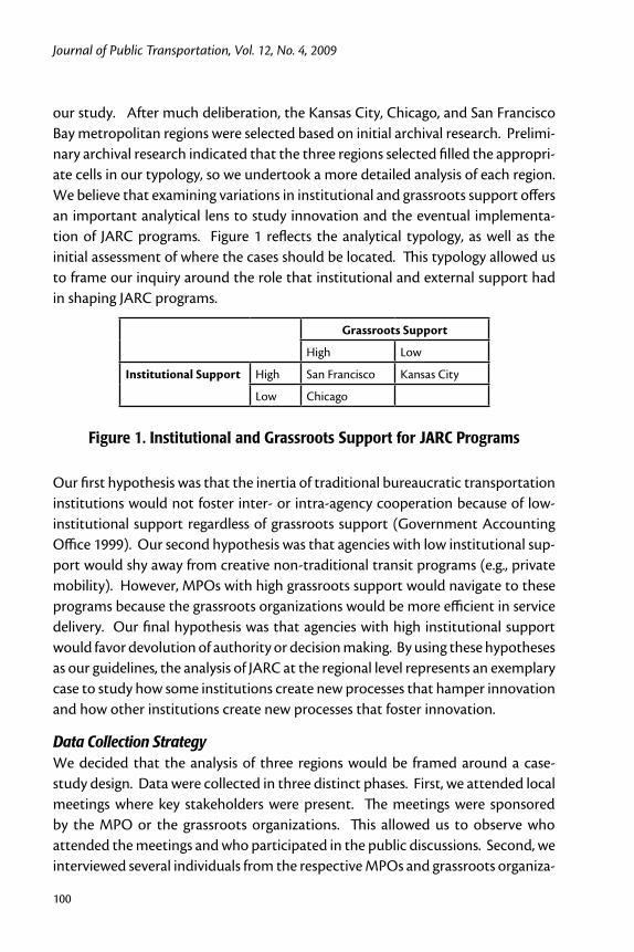
Journal of Public Transportation, Vol. 12, No. 4, 2009
100
our study. After much deliberation, the Kansas City, Chicago, and San Francisco Bay metropolitan regions were selected based on initial archival research. Prelimi-nary archival research indicated that the three regions selected filled the appropri-ate cells in our typology, so we undertook a more detailed analysis of each region. We believe that examining variations in institutional and grassroots support offers an important analytical lens to study innovation and the eventual implementa-tion of JARC programs. Figure 1 reflects the analytical typology, as well as the initial assessment of where the cases should be located. This typology allowed us to frame our inquiry around the role that institutional and external support had in shaping JARC programs.
Grassroots Support
High Low
Institutional Support High San Francisco Kansas City
Low Chicago
Figure 1. Institutional and Grassroots Support for JARC Programs
Our first hypothesis was that the inertia of traditional bureaucratic transportation institutions would not foster inter- or intra-agency cooperation because of low-institutional support regardless of grassroots support (Government Accounting Office 1999). Our second hypothesis was that agencies with low institutional sup-port would shy away from creative non-traditional transit programs (e.g., private mobility). However, MPOs with high grassroots support would navigate to these programs because the grassroots organizations would be more efficient in service delivery. Our final hypothesis was that agencies with high institutional support would favor devolution of authority or decision making. By using these hypotheses as our guidelines, the analysis of JARC at the regional level represents an exemplary case to study how some institutions create new processes that hamper innovation and how other institutions create new processes that foster innovation.
Data Collection StrategyWe decided that the analysis of three regions would be framed around a case-study design. Data were collected in three distinct phases. First, we attended local meetings where key stakeholders were present. The meetings were sponsored by the MPO or the grassroots organizations. This allowed us to observe who attended the meetings and who participated in the public discussions. Second, we interviewed several individuals from the respective MPOs and grassroots organiza-
A Case Study of Job Access and Reverse Commute Programs
101
tions. Most of the interviews were done face-to-face. However, a few interviews were conducted by telephone because of logistical issues. The interviews were not taped, but we took notes that highlighted the important themes that emerged from the interviews. Finally, we collected published reports, newspaper articles, and public documents that were related to JARC programs in each region. The documents were systematically organized to study innovation, implementation, grassroots support, and institutional support.
The Chicago CaseThe Chicago metropolitan area was well positioned to qualify for JARC funding when the program was announced. Due to pressure from community groups, the Chicago Area Transportation Study (CATS), the MPO for the region, established the Community Mobility Task Force. This task force was created to study the mobility needs of the poor, particularly access to job opportunities for the unem-ployed.4 In 1998-99, the Task Force had 21 members, including the Illinois Depart-ment of Transportation (IDOT), the Illinois Department of Human Services, the City of Chicago, the Councils of Mayors, the three public transit agencies, private transportation providers, social service agencies, and community based organiza-tions (e.g., The Center for Neighborhood Technology [CNT]).
As the FTA worked on guidance, the Task Force continued to meet and consider early candidates for JARC funds, including an expansion of the Metra Shuttle Bug service and a bus service to take residents from the South suburbs to industrial jobs around O’Hare Airport (Chicago Area Transportation Study 1998). In Octo-ber, the FTA guidance for the program was released. At that time, MPOs were informed that the applications for JARC funds were due by December 31, a very short lead time for such an important program, which was then cut further by two weeks due to the need to have the grant proposal ready for approval by the CATS Policy Committee (Chicago Area Transportation Study 1998). In October, the Task Force hosted a workshop for non-traditional transportation providers to explain the program and to solicit proposals for JARC funding. One general finding was that participation in the Task Force was erratic. Many of the core task force members attended nearly all meetings, but smaller transit providers or average citizens appeared only when there was a chance that new projects would be selected for inclusion in an official CATS submittal. Participation dropped off as it became clear that new projects would be shut out due to the high levels of federal earmarking.
Journal of Public Transportation, Vol. 12, No. 4, 2009
102
It became apparent to the Task Force that the local match requirement (a full 50%) was an insurmountable barrier for the vast majority of the small transpor-tation companies unless they had partnered with a government agency, such as the City of Chicago or DuPage County. Of the 14 projects that were submitted, those projects not connected to a government agency were often grouped into a catchall project called the Chicago Area Job Access and Transit Enhancement Plan, which would be administered by the CTA, Metra, and Pace.
After evaluating the proposals, the Task Force pulled together its grant proposal. The proposal included eight first-tier projects at a total cost of $2.5 million, with $1.5 programmed for the Chicago Area Job Access and Transit Enhancement Plan. There were three second- and third-tier projects, which were requests for second year funding for several of the first-tier projects (Chicago Area Transporta-tion Study 1998). It appears that when the FTA analyzed the grant proposal, the agency ran down the list and accepted the first five-first tier projects for a total grant of $2.2 million and dropped the remainder, for the award amounts for FY 1999 closely matched the CATS’ figures in the proposal.
Northeastern Illinois continued to receive a considerable share of JARC funds for FY 2000 through FY 2002. In all three years, the total grants were over $2 million. However, due to Congressional earmarking, CATS and the Community Mobility Task Force had less and less control over how the funds were allocated. For exam-ple, of the $2.2 million for FY 2000, CATS had only $1 million to distribute. The funds to be spent on direct transportation services for the poor were cut roughly in half, though of course the region still had a considerable sum of unobligated funds from FY 1999. The funding picture was similar for FY 2000, where roughly $2 million was available for the Chicago metropolitan region, but $1.5 million had come from various earmarks. By FY 2002, nearly 90 percent of JARC funds were allocated according to earmarks, though the Chicago area still won some of the competitive grants, but by FY 2003, the entire federal JARC program had been earmarked. Chicago’s share dropped to under $0.5 million (See Table 1). When examined on a per capita basis, the Kansas City and San Francisco regions received nearly four times the JARC funding as Chicago, which can be attributed almost entirely to earmarks. This is a curious outcome, given that, at both the central city level and regional level, Chicago’s poverty rate exceeds that of Kansas City or San Francisco.

A Case Study of Job Access and Reverse Commute Programs
103
Table 1. JARC Funding ($ millions) in Metropolitan Chicago, Kansas City and San Francisco
Note: FY 2003-05 Chicago figures does not include statewide Illinois Ways to Work funding Source: CATS, MARC, MTC, US GAO, US Census
One CATS official responsible for oversight of the Community Mobility Task Force’s proposal commented that the heavy use of earmarks in the last years of the program made it a different program. Most agencies nationwide that asked their Congressional representatives for JARC earmarks did receive them, but in the Chi-cago region only PACE, UIC, and DuPage County made that effort. This person did not speculate on why CTA and Metra did not seek out earmarks, though it could well be that those agencies were already asking Congress to fund massive infra-structure projects that had a higher internal priority than the JARC programs.
In giving a general evaluation of the program, one local observer from the Center for Neighborhood Technology felt that the JARC program was very important for simply trying to meet the transportation needs of the poor. This person felt that there was considerable pent-up demand for non-traditional transit service specifi-cally targeted at welfare recipients and other low-income individuals. This person would have liked more flexibility in the program, particularly when it came to the FTA requirements, but a more critical need was to ensure that there was ongoing support for worthy JARC programs, since agencies generally were not willing to commit themselves to sustaining reverse commute programs in the absence of external funds. The program should have been structured to guarantee the oper-ating funds for a longer time in order to build demand for transit in the region; even a three-year pilot program was not really long enough.
Journal of Public Transportation, Vol. 12, No. 4, 2009
104
The San Francisco CaseThe situation in the Bay Area was similar to that in Chicago in terms of the MPO applying for a large JARC grant to support a transit-oriented plan. In addition, in both regions, a fair number of stakeholders took part in the process. After the passage of California’s CalWORKs law in 1997, the Metropolitan Transportation Commission (MTC) took a leadership role to address the transportation barriers that poor women would encounter as they looked for work. Because MTC is the transportation planning, coordinating, and financing agency for the San Francisco Bay region, they were in a unique position to lead the planning process and iden-tify regional transit problems and solutions.
In 1998, with the support of MTC, AC Transit started an experimental bus line that operated during evening hours to connect welfare recipients in Richmond to employment centers that had job openings for shift workers. This was the first program enacted that specifically addressed a key transportation barrier for Cal-WORK recipients. The goal of the service was to provide more transit access to Richmond, which had one of the highest concentrations of CalWORK recipients, to areas that had a shortage of entry-level employees. In the eyes of MTC and AC Transit, the “OWL” service was a success because it was providing a service to residents and the service was being used by the residents. Success in this context is relative. In fact, when asked to define success, the officials from MTC simply stated that the “OWL” service was a success because it was used by underserved low-income populations regardless of the cost.5
MTC coordinated all the JARC applications by grassroots organizations to ensure that there were no duplications in services. One of the most innovative programs funded with JARC funds was the regional JARC program, the Low-Income Flexible Transportation program (LIFT). LIFT provided funding to fill transportation gaps that had been identified through local and regional welfare-to-work planning workgroups with grassroots organizations. One major goal of LIFT was to secure JARC funding for grassroots organizations to ensure that these organizations had the opportunity to be co-planners, co-designers, and co-implementers of innova-tive JARC programs.
Taking advantage of JARC’s flexibility, in the first round, MTC funded two projects designed to provide transportation for children and one project designed to pro-vide non-traditional transportation access. One reason there was a low number of these projects was that they required more time and coordination from MTC staff. Another reason there was a low number of applications was because it took
A Case Study of Job Access and Reverse Commute Programs
105
a significant amount of time to clarify JARC program objectives and regulations and identify resources that could be used to ensure that the program would work. Even though half of the LIFT programs were for bus line improvements, MTC recognized that public transit could not meet the needs of all CalWORK recipients (Fol et al. 2007). This was a new and awkward position for MTC given that their overall mission is to promote public transit (Fol et al. 2007; Blumenberg et al. 2003). By funding two car programs and one vanpool program in the sec-ond round of LIFT funding, MTC took a step towards increasing the diversity of transit options for low-income populations. Studies have consistently shown that welfare recipients that own a car are more likely to leave the welfare rolls and find sustainable employment (Lucas and Nicholson 2003; Cervero et al. 2002; O'Regan and Quigley 1998; Blumenberg 2000; Cervero et al. 2002; Ong and Blumenberg 1998; Ong 1996; Raphael and Rice 2002). Another study found that even those welfare recipients who found employment using public transportation would immediately buy a car when they have saved enough money for the down pay-ment (Blumenberg 2000).6
More significantly, MTC increased funding for transportation services specifically targeted at children of low-income families. These types of services have become increasingly important as single women with children try to reduce the number of multi-leg work commutes to simple one-leg commutes, thus reducing the amount of time they have to spend on commuting and transferring from bus line to bus line to get from their home to work. Perhaps one of the most innovative uses of LIFT funding was a program in Sonoma County called Long-Term Transportation Solutions. One component of this program was teaching welfare recipients how to make complex trips via public transit more efficient. Many entry-level job openings for Sonoma County residents are located in San Rafael in Marin County. Getting to these jobs via public transit is possible, but bad trip planning can result in a passenger spending unnecessary hours on public transit. Learning how to read a transit system and plan appropriately for bus transfers is essential for residents in the North Bay, where bus service is not as frequent as service in the East Bay.
The Kansas City CaseThe MPO for the Kansas City area is the Mid-America Regional Council (MARC). In contrast to Chicago, the initial response from established transit agencies in Kansas City when the opportunity for JARC funding arose was to compete against each other for funding. The JARC funding regulations had specified a single fund-

Journal of Public Transportation, Vol. 12, No. 4, 2009
106
ing application come from each region, so the transit agencies still had to work through the MPO rather than to submit separate applications to FTA directly. This presented MARC with a choice of submitting a laundry list of six or seven unrelated projects or trying to present a unified plan that might be more compel-ling to FTA. MARC attempted the latter approach and, within a month, pulled together a consortium of area transportation providers, municipalities, and social service organizations to create the Kansas City Areawide Job Access Partnership, which became an advisory council under MARC’s committee structure. Many of the participants already were members of the Special Transportation committee, which addressed the transportation needs of the elderly and disabled populations in the Kansas City metropolitan area (Special Transportation Advisory Committee 1992). The original members were MARC, the Kansas City Area Transit Authority (KCATA) (Missouri), Unified Government Transit (UGT) (Kansas City, Kansas and Wyandotte County), Johnson County Transit, Full Employment Council, OATS (a rural transportation provider), and Ray County Transit.
In developing the consolidated, multi-year JARC application, MARC officials and committee participants reported that there were already-known transportation needs that were not being addressed and special challenges facing the Kansas City region, if it wished to compete for JARC funding. Despite four transit service providers in the region (KCATA, Johnson County Transit, Ray County Transit, and OATS), there was no dedicated revenue source to fund transit. In addition to making it much harder to develop a funding stream for the local match provision in the JARC application, the participants were concerned about the possibility of implementing services that would then be lost after the federal funding was gone. Thus, there were efforts early on to enlist employer-support for JARC services in an attempt to make the new services self-sustaining.
Metropolitan Kansas City benefitted substantially from the earmarking process. A Kansas congressman liberally earmarked JARC funds for his region. During the five years of the TEA-21-legislated JARC program, he acquired $2,000,000 for the Job Access Partnership to support job access transportation in Johnson County and $4,625,000 for the Unified Government. He also secured an earmark of $500,000 for UG in the reauthorized transportation bill SAFETEA-LU (Mid-America Regional Council 2005).
An official from Unified Government Transit reported that the earmarked funding was used to offset the cost of its annual contract with KCATA for transit service.
A Case Study of Job Access and Reverse Commute Programs
107
KCATA provides 850,000 passenger trips in Wyandotte County plus transporta-tion between Kansas and Missouri. UGT also participates in the JARC Partnership because of its regional focus, for which it receives $45,000 annually. Through 2004, these funds were used for UGT’s Joblinks program, which was contracted service to provide transportation to Wyandotte County residents who worked in Johnson County, at locations that either had no bus service or no service during the rider’s work shift. About 33,000 annual trips were provided with this service. Recently, the transit service subsidized with JARC funding was shifted to serve an area of Wyandotte County that has a NASCAR track and an adjacent 400 acres that the County has retained for future development. Over 2,500 job opportunities are anticipated in the area.
DiscussionIn Chicago, implementing the various JARC projects turned out to be considerably more challenging than winning the awards. It turned out that few (if any) FTA regulations had been reduced or relaxed for non-traditional providers involved in the projects. This ultimately led to the Regional Transportation Authority act-ing in an oversight capacity to ensure that all FTA requirements would be met to prevent violations that might result in lost funding. Since this relationship had not been completely worked out prior to the submittal of the JARC grant application, it took time to set it up. Staff turnover at RTA also hampered the implementa-tion of the program. While some JARC funds were expanded in 2000, it was clear that the program was severely delayed, above and beyond the nine month lag that most projects faced. The U.S. DOT noted that by mid 2001, only seven projects had been selected for grants in FY 1999 where the funds had still not been fully obligated, and five of them were in the Chicago area—essentially the entire CATS proposal (Chicago Area Transportation Study 1998).
Chicago was objectively slower in using JARC funds than other metropolitan regions, which might have led to the frustration some grassroots organizations had with the program. The meeting minutes from the Community Mobility Task Force often present grassroots organizations attempting to hold transit agencies responsible for previous JARC obligations. In some cases, pressure from these grassroots organizations appeared to keep a few JARC programs running longer. Nonetheless, the relationship between the transportation planners and the grassroots organizations was somewhat strained over the JARC process, and a certain amount of defensive blame-avoidance was observed. From our research,
Journal of Public Transportation, Vol. 12, No. 4, 2009
108
it appears that devoting more effort to maintain and improve these relationships would have not produced more institutional support for innovative JARC proj-ects.
Table 1 indicated that Chicago had the lowest institutional support (at the federal level) of the three MPOs studied. Earmarks were not a high priority for Chicago’s Congressional representation, and JARC funding went to other regions with smaller impoverished populations (in absolute and relative terms). The imple-mentation of JARC-funded projects went the most smoothly when run through transit service boards (i.e., between official agencies) and the grassroots efforts stalled. Metra, Pace, and the CTA all were able to report new JARC-supported service on the ground by December 2000.
The lessons learned in Chicago appear to be that non-traditional companies were not well positioned to administer JARC programs on their own or even with the assistance of the RTA. Successful partnerships were possible where a smaller com-pany partnered with CTA, Metra, or Pace.7 One potential solution of the Access-to-Jobs program would have been for the FTA to undergo a cultural change, mak-ing them more willing to accept nontraditional approaches for addressing welfare-to-work barriers (Government Accounting Office 1998). Many observers contend that this cultural shift did not occur and made implementing the program more difficult. Additional institutional support presumably would have allowed RTA to overcome these barriers (as MTC was able to do). In short, MTC was more active than CATS in actively pursuing inter-agency collaboration with grassroots orga-nization. The synergy of inter-agency collaboration gave MTC more institutional support to use JARC funding in a more creative way.
In contrast to Chicago, both the San Francisco Bay Area and Kansas City received large earmarks, indicating considerable institutional support. The respective MPOs had quite different outcomes in terms of success in engaging the grassroots. First, as MTC worked with grassroots organizations, three objectives were identified to address the transportation barriers: (1) “assess the transportation requirements of CalWORKs program participants and identify transportation-related barriers to obtaining and retaining work,” (2) “identify strategies to increase availability, affordability, and effectiveness of transportation services,” and (3) “establish agreements among the transportation providers, employers and Social Services Agency (SSA) to ensure the availability of Transportation options” (Stewart 1999). As mentioned previously, MTC recognized that traditional public transit services could not solve all the transportation needs for welfare recipients. MTC was the
A Case Study of Job Access and Reverse Commute Programs
109
only region that worked aggressively with grassroots organizations to sponsor sev-eral non-traditional transportation projects with JARC funds (e.g., car programs and vanpool programs). The strong grassroots support allowed MTC to create innovative, non-traditional transportation programs to meet the unorthodox transportation needs of welfare-to-work recipients.
It is important to note that although MTC considered the LIFT program to be a success, it expressed concern about institutional and programmatic barriers that interfered with the coordination of welfare-to-work and job access programs. MTC consistently encountered programmatic barriers, a lack of flexibility in JARC guidelines, and a failure by FTA to answer questions regarding JARC guidelines in an appropriate time-frame. As far as the institutional barriers were concerned, MTC found that it was difficult to maintain momentum with welfare-to-work plans. MTC applauded JARC’s focus on coordination but found it difficult to coor-dinate JARC activities with a diverse group of grassroots organizations providing services for CalWORK recipients. Trying to coordinate with a diverse group was time-consuming, and it was difficult to build consensus, given that the organiza-tions have different goals. Despite these challenges, MTC and the grassroots orga-nizations worked to create innovative programs that could be implemented.
In the Kansas City region, grassroots support was missing. In the first round of JARC funding, no grassroots organizations were reported to have requested JARC funding. In fact, there was no RFP process in the Kansas City region to invite groups that did not have a seat on the committee to participate in the JARC program until Year 4, for which the Partnership set aside 20 percent of the JARC funds for new projects. The co-chair of the Special Transportation Committee reported that by the second application (second two-year program), the Partner-ship knew where to beef up existing services because of the variety of interests on the committee. By this time, the committee had more consumer representation, and the JARC Partnership and the committee that previously focused on senior citizens and the disabled population merged into a single Special Transit Com-mittee, greatly expanding the number of participants. The MPO and all but one member of the committee could list no grassroots organizations that pushed for JARC funding. Much of the transportation advocacy work in the area has been in reference to encouraging legislators to create a stable funding source for transit or advocating for light rail. Such organizations include the Regional Transit Alliance and Citizens for Modern Transit. In contrast to the situations in Chicago and San Francisco, community groups in Kansas City did not play an active role in putting
Journal of Public Transportation, Vol. 12, No. 4, 2009
110
the proposal together nor watching over how the funds were spent. In general, community groups did not take an active role in following or trying to influence planning decisions taken by MARC.
One group did try to fill the role of a grassroots organization, the Local Investment Commission (LINC), a community collaborative that works to improve the lives of children and families in Jackson County. It is important to note that LINC worked with community-based agencies that were seeking JARC funds, served in an advi-sory role to the committee, and provided matching funds for community groups, whose projects had been implemented. LINC also worked with Ford and com-munity programs to help low-income workers obtain loans for autos. Based on the Kansas City case, we modified our first hypothesis to indicate that institutional support is a necessary, but not sufficient, condition for innovation. The MPO had considerable support on the JARC issue and should have been able to work with any partner, but it was not met with any offers to establish non-traditional transit service. As illustrated in Figure 1, San Francisco was the only region that had high institutional and high grassroots support. Chicago had high grassroots support but insufficient institutional support. Kansas City had high institutional support but lacked grassroots support.
ConclusionsWe framed this paper around two issues: (1) institutional support and (2) grass-roots support. Our analysis shows the Chicago, Kansas City, and San Francisco MPOs responded in different ways. We believe that the policy outcomes reflected the intensity of institutional and grassroots support to use JARC as an opportu-nity to create innovative transportation programs for low-income populations. In regards to our analytical typology of support, MTC was the only region with high institutional and grassroots support; thus, it was in a unique position to actively pursue private mobility programs for low-income families. Although these programs were discussed for the Chicago region, CATS did not provide the type of institutional support that MTC provided. Although the Kansas region had the institutional support for such creativity, it lacked the grassroots support for private mobility programs. In fact, MTC’s support for these car-sharing programs showed that they recognized that the structural barriers could not be overcome by fixed transit service. By recognizing that public transit was simply not flexible
A Case Study of Job Access and Reverse Commute Programs
111
enough to meet all the needs of CalWORK recipients, MTC opened an important avenue of private mobility services that, in the long-run, foster a policy environ-ment that is conducive to sustainable economic self-sufficiency. MTC’s vision reflects the new collective rationality that investing in private mobility programs is a greater good than continually investing in public transit programs where there is no long-term bang for the buck.
Finally, alone among the MPOs we studied, MTC spearheaded an effort to create a regional JARC program to allow smaller non-traditional transportation providers to apply for federal money. MTC created social processes in which some author-ity and project management was given to grassroots organizations. Thinking more broadly about creativity, institutional creativity often requires sufficient funding (that has not been narrowly restricted to particular uses), and in the later fiscal years of the JARC program, the rules had changed to the point where substantial funding was only available when there was high institutional support from national-level politicians. While the institutional support appears to be a necessary condition, it is not sufficient, or more innovation would have occurred in Kansas City. The combination of institutional and grassroots support was what allowed MTC to be the most innovative region.
End Notes1 Policy experts warned that transportation was not a panacea to lower welfare rates. Other needs, such as access to child care or basic skill training, are just as crucial for welfare recipients as they try to find jobs (see Wachs and Taylor 1998).
2 See Douglas (1986) for an expanded discussion of rational choice theory and functional theory.
3 Bureaucratic agencies (or rather, the bureaucrats staffing them) are often moti-vated more by blame-avoidance than the more positive (and potentially construc-tive) credit-seeking role that can be activated by public support for new policies and programs (Lee 1994). Indeed, it is worth considering whether innovation in itself is likely to provoke blame-avoidance as a preemptive strategy and what may be done to limit this response.
4 The process of instituting the Community Mobility Task Force began in June 1997, but it took several months to determine its composition. The Task Force is unique among CATS’ working groups, since it is the only one to be chaired (in fact,
Journal of Public Transportation, Vol. 12, No. 4, 2009
112
co-chaired) by citizen representatives rather than a representative of the govern-ment or a transportation provider. This structure was requested by a variety of community and environmental groups in Chicago.
5 Scholars have found that the 376 line cost $7 per passenger trip versus a fare of $1.50 (Sööt et al. 2002).
6 Reverse commute programs that are measured on ridership (rather than people removed from welfare rolls) will inevitably spend more resources chasing potential riders as the original riders opt out of the service after a few months of employ-ment when they are able to buy a car (Petersen and Sermons 1996).
7 The DuPage Federation, which had earmarks in all years after FY 1999, did work with smaller companies.
References
Altshuler, A. A. , and R. D. Behn, eds. 1997. Innovation in American Government: Challenges, Opportunities, and Dilemmas. Edited by A. A. Altshuler and R. D. Behn. Washington D.C.: Brookings Institution Press.
Blumenberg, E. 2000. Moving welfare participants to work: Women, transporta-tion, and welfare reform. Affilia 15(2): 259-276.
Blumenberg, E., D. Miller, M. Garrett, L. Schweitzer, K. Kitsis, M. Manville, and B. Mallavarapu. 2003. California transportation needs assessment: The trans-portation barriers and needs of welfare recipients and low-wage workers. The Ralph & Goldy Lewis Center for Regional Policy Studies, UCLA School of Public Policy and Social Research.
Blumenberg, E. 2002. Planning for the transportation needs of welfare participants: Institutional challenges to collaborative planning. Journal of Planning Educa-tion and Research 22(2): 152-163.
Blumenberg, E., and M. Manville. 2004. Beyond the spatial mismatch: Welfare recipients and transportation policy. Journal of Planning Literature 19(2): 182-205.
Blumenberg, E., and L. Schweitzer. 2006. Devolution of transport policy for the working poor: The case of the U.S. Job Access and Reverse Commute Program. Planning Theory and Practice 7: 7-25.
A Case Study of Job Access and Reverse Commute Programs
113
Cervero, R. 2004. Job isolation in the U.S.: Narrowing the gap through Job Access and Reverse-Commute Programs. In Running on Empty: Transport, Social Exclusion and Environmental Justice, edited by K. Lucas. Bristol, UK: Policy Press.
Cervero, R., J. O. Sandoval, and J. Landis. 2002. Transportation as a stimulus of welfare-to-work: Private versus public mobility. Journal of Planning Education and Research 22: 50-63.
Cervero, R., and Y. Tsai. 2003. Job access and reverse commute initiatives in Califor-nia: A review and assessment. Transportation Research Record 1859: 76-86.
Cervero, R., Y. Tsai, M. Wachs, E. Deakin, J. Dibb, A. Kluter, C. Nuworsoo, I. Petrova, and M. Pohan. 2002. Reverse commuting and job access in California: Mar-kets, needs, and policy prospects. In Institute of Transportation Studies. UCB-ITS-RR-2002-7 Berkeley, CA.
Chicago Area Transportation Study. 1998. Regional job access and reverse com-mute transportation plan and grant application for Northeastern Illinois. Chicago.
DiMaggio, P. L., and W. W. Powell. 1991. The iron cage revisited: Institutional isomorphism and collective rationality in organizational fields. In The New Institutionalism In Organizational Analysis, edited by W. W. Powell and P. L. DiMaggio. Chicago, IL: The University of Chicago Press.
Douglas, M. 1986. How Institutions Think. Syracuse, NY: Syracuse University Press.
Fol, S., G. Dupuy, and O. Coutard. 2007. Transport policy and the car divide in the UK, the U.S. and France: Beyond the environmental debate. International Journal of Urban and Regional Research 31 (4):802-812.
Forester, J. 1989. Planning in the Face of Power. Berkeley, CA: University of Califor-nia Press.
Gomez Ibanez, J. 1984. Transportation and the poor. In The State and the Poor in the 1980, edited by M. Carballo and M. J. Bane. Boston, MA: Auburn House.
Government Accounting Office. 1998. Welfare reform: Implementing DOT’s Access to Jobs Program. In GAO RCED 99-36.
Government Accounting Office. 1998. Welfare reform: Transportation’s role in moving from welfare to work. In GAO RCED 98-161.
Journal of Public Transportation, Vol. 12, No. 4, 2009
114
Government Accounting Office. 1999. Welfare reform: Implementing DOT’s Access to Jobs Program in its first year In GAO RCED 00-14.
Kasarda, J. 1988. Jobs, migration, and emerging urban mismatches. In Urban Change and Poverty, edited by M. McGeary, G. H. and L. E. Lynn. Washington, DC: National Academy Press.
Lee, S. 1994. Policy type, bureaucracy, and urban policies: Integrating model of urban service distribution. Policy Studies Journal 22: 87-108.
Lieberman, R. C., and G. M. Shaw. 2000. Looking inward, looking outward: The poli-tics of state welfare innovation under devolution. Political Research Quarterly 53(2): 215-240.
Lucas, M. T., and C. F. Nicholson. 2003. Subsidized vehicle acquisition and earned income in the transition from welfare to work. Transportation 30(4).
Mid-America Regional Council. 2005. Congressman Dennis Moore secures funds to provide job access and reverse commute services for region. MARC 2005 [cited February 10 2005].
O’Regan, K., and J. Quigley. 1998. Cars for the poor. Access 12.
Ong, P., and E. Blumenberg. 1998. Job access, commute and travel burden among welfare recipients. Urban Studies 25(1): 77-93.
Ong, P. 1996. Work and automobile ownership among welfare recipients. Social Work Research 20(4): 193-288.
Ortoleva, S., and M. Brenman. 2004. Women’s issues in transportation. In Running on Empty: Transport, Social Exclusion and Environmental Justice, edited by K. Lucas. Bristol, UK: Policy Press.
Petersen, E., and M. Sermons. 1996. Evaluating reverse commute programs in Chi-cago. In Metropolitan Conference on Public Transportation Research. Chicago.
Raphael, S., and L. Rice. 2002. Car ownership, employment, and earnings. Journal of Urban Economics 52: 109-130.
Sanchez, T. W., Q. Shen, and Z. R. Peng. 2004. Transit mobility, jobs access, and low-income labor participation in U.S. Metropolitan Areas. Urban Studies 41(7): 1313-1331.
A Case Study of Job Access and Reverse Commute Programs
115
Sanchez, T.W., R. Stolz, and J. Ma. 2003. Moving to equity: Addressing inequitable effects of transportation policies on minorities. Cambridge, MA: The Civil Rights Project at Harvard University.
Sanchez, T. W., and L. Schweitzer. 2008. Assessing federal employment accessibil-ity policy: An analysis of the JARC Program. In Metropolitan Policy Program. Washington D.C.: Brookings.
Schram, S. F. 1998. Introduction to welfare reform: A race to the bottom. Publius 28(3): 1-7.
Singh, J. V., D J. Tucker, and A. G. Meinhard. 1991. Institutional change and ecologi-cal dynamics. In The New Institutionalism In Organizational Analysis, edited by W. W. Powell and P. L. DiMaggio. Chicago, IL: The University of Chicago Press.
Sööt, S., P. Sriraj, and P. Thakuriah. 2002. A user survey of transportation services funded by the Job-Access-Reverse-Commute Program. Chicago, IL: Urban Transportation Center.
Special Transportation Advisory Committee. 2005. Memorandum. MARC, March 5, 2005 1992 [cited March 5 2005].
Stewart, L. 1999. Welfare to work: The transportation issue. Bay Area Monitor.
Wachs, M., and B. D. Taylor. 1998. Can transportation strategies help meet the welfare challenge? Journal of the American Planning Association 64(1): 15-19.
Weber, M. [1922] 1978. Economy and Society. Berkeley, CA: University of California Press.
About the Authors
J.S. Onésimo Sandoval ([email protected]) is an Assistant Professor in the Department of Sociology and Criminal Justice. He received his Ph.D. from the University of California, Berkeley.
Eric Petersen ([email protected]) is an Associate at Cambridge Systematics. He received his Ph.D. from Northwestern University.
Kim L. Hunt ([email protected]) is a principal with the O-H Community Partners, Ltd.
Journal of Public Transportation, Vol. 12, No. 4, 2009
116
117
Design of Transit Signal Priority at Signalized Intersections with Queue Jumper Lanes
Design of Transit Signal Priority at Signalized Intersections with
Queue Jumper Lanes Guangwei Zhou, HDR Engineering, Inc.
Albert Gan, Florida International University
Abstract
A queue jumper lane is a special bus preferential treatment that combines a short stretch of a special lane with a transit signal priority (TSP) to allow buses to bypass waiting queues of traffic and then to cut out in front of the queue by getting an early green signal. This paper first proposes a signal control design for queue jumper lanes with actuated TSP strategies and then compares its performance with that of the general actuated mixed-lane TSP. Different design alternatives were evaluated in the VISSIM microscopic simulation. The results show that the proposed TSP with queue jumper lanes can reduce more bus delays than can the commonly-used mixed-lane TSP, especially under high traffic volume conditions. It was also found that a near-side bus stop is superior to the far-side counterpart in terms of both bus delay and overall intersection delay for the proposed design.
IntroductionThe provision of transit signal priority (TSP) on arterial streets is a transit pref-erential treatment that has received increasing attention in North America. In practice, however, studies have shown that TSP is ineffective during peak hours because buses are not able to bypass the long waiting queues during these hours
Journal of Public Transportation, Vol. 12, No. 4, 2009
118
(Nowline 1997; Head 1998; Balke 2000). This paradox has had a limiting effect on the applications of TSP in practice.
A special type of bus preferential treatment that has the potential of avoiding this weakness is queue jumper lanes. A queue jumper lane combines a short stretch of a special lane, such as a right-turn lane, with signal priority to allow buses to bypass a waiting queue of traffic and then to cut out in front of the queue by get-ting an early green signal. Figure 1 shows an intersection with a standard queue jumper lane design. A queue jumper lane can essentially operate like a bus lane at the vicinity of an intersection. However, unlike bus lanes, a queue jumper lane does not take a lane away from the general traffic, making its implementation easier to justify. Instead, a queue jumper lane makes full use of an existing right- or left-turn bay that generally operates under low saturation conditions. In addition, the queue-bypassing capability of a queue jumper lane can avoid the queue uncer-tainties that limit the effectiveness of mixed-lane TSP, especially under congested conditions. When implemented with TSP, hereafter referred to as the jumper TSP, a queue jumper lane can potentially be more effective than a typical mixed-lane TSP and be more feasible than bus lanes (Zhou 2005, 2006).
While the queue bypassing capability of a queue jumper lane is similar to that of a bus lane, the operations of a queue jumper lane are quite different from a bus lane and deserve separate design considerations. Unlike a bus lane, a queue jumper lane requires that buses yield and wait for an acceptable gap to merge back into the main flow downstream. Consequently, the design of jumper TSP, including both the phasing and phase split, is also very different from that of bus lanes or mixed-lane TSP strategies.
The objectives of this paper are twofold. The first objective is to propose an actu-ated TSP strategy and its associated signal control designs for a queue jumper lane. In an actuated TSP strategy, a priority signal is provided only when a request from a bus is detected. The second objective is to evaluate the performance of the proposed queue jumper TSP strategy by comparing it with the general actuated mixed-lane TSP. The next section presents the design of various signal design ele-ments for TSP and queue jumper lanes, including phasing, phase splits, multiple bus services, and coordination recovery and green reimbursement. This is followed by the implementation of the proposed designs in a simulation testbed for a performance evaluation with mixed-lane TSP. The results are then presented and conclusions drawn.
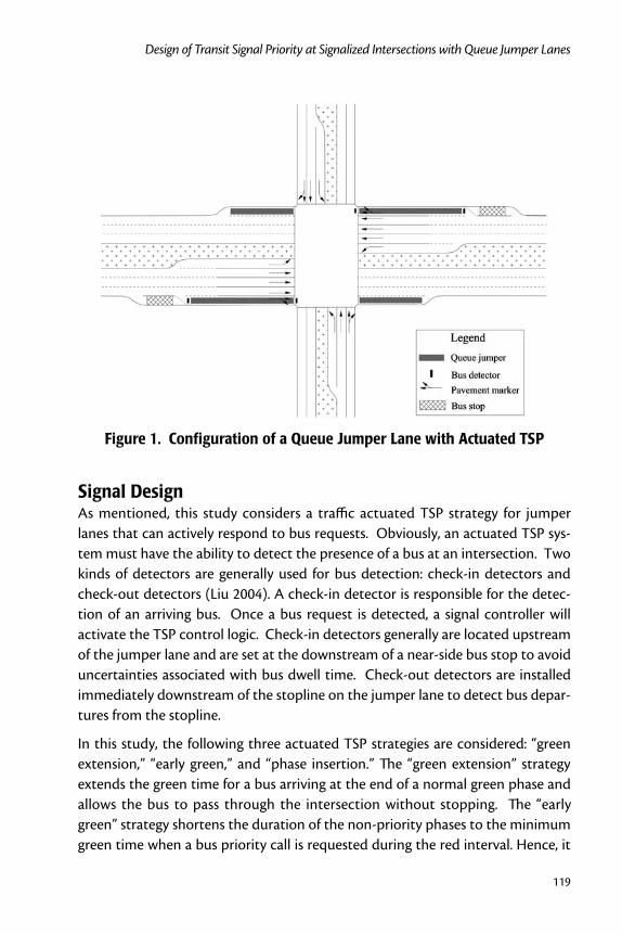
119
Design of Transit Signal Priority at Signalized Intersections with Queue Jumper Lanes
Figure 1. Configuration of a Queue Jumper Lane with Actuated TSP
Signal Design As mentioned, this study considers a traffic actuated TSP strategy for jumper lanes that can actively respond to bus requests. Obviously, an actuated TSP sys-tem must have the ability to detect the presence of a bus at an intersection. Two kinds of detectors are generally used for bus detection: check-in detectors and check-out detectors (Liu 2004). A check-in detector is responsible for the detec-tion of an arriving bus. Once a bus request is detected, a signal controller will activate the TSP control logic. Check-in detectors generally are located upstream of the jumper lane and are set at the downstream of a near-side bus stop to avoid uncertainties associated with bus dwell time. Check-out detectors are installed immediately downstream of the stopline on the jumper lane to detect bus depar-tures from the stopline.
In this study, the following three actuated TSP strategies are considered: “green extension,” “early green,” and “phase insertion.” The “green extension” strategy extends the green time for a bus arriving at the end of a normal green phase and allows the bus to pass through the intersection without stopping. The “early green” strategy shortens the duration of the non-priority phases to the minimum green time when a bus priority call is requested during the red interval. Hence, it
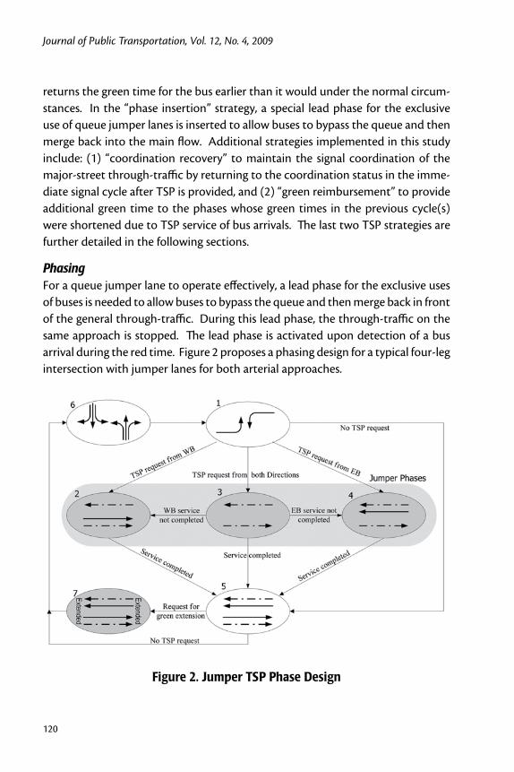
Journal of Public Transportation, Vol. 12, No. 4, 2009
120
returns the green time for the bus earlier than it would under the normal circum-stances. In the “phase insertion” strategy, a special lead phase for the exclusive use of queue jumper lanes is inserted to allow buses to bypass the queue and then merge back into the main flow. Additional strategies implemented in this study include: (1) “coordination recovery” to maintain the signal coordination of the major-street through-traffic by returning to the coordination status in the imme-diate signal cycle after TSP is provided, and (2) “green reimbursement” to provide additional green time to the phases whose green times in the previous cycle(s) were shortened due to TSP service of bus arrivals. The last two TSP strategies are further detailed in the following sections.
PhasingFor a queue jumper lane to operate effectively, a lead phase for the exclusive uses of buses is needed to allow buses to bypass the queue and then merge back in front of the general through-traffic. During this lead phase, the through-traffic on the same approach is stopped. The lead phase is activated upon detection of a bus arrival during the red time. Figure 2 proposes a phasing design for a typical four-leg intersection with jumper lanes for both arterial approaches.
Figure 2. Jumper TSP Phase Design
121
Design of Transit Signal Priority at Signalized Intersections with Queue Jumper Lanes
In the phase diagram, the movements for queue jumper lanes are shown with dashed lines and the movements for the normal lanes are shown with solid lines. The three non-shaded phases (phases 1, 5, and 6) are used under normal condi-tions when the jumper TSP is not activated. The three shaded phases (phases 2, 3, and 4) are jumper phases designed for various bus requests during the red time from both directions of the arterial. Either phase 2 or phase 4 is activated when bus requests occur only on one arterial approach. When buses are detected on both arterial approaches simultaneously, phase 3 is activated. At the end of phase 3, if there are still bus requests that are not served in either jumper lane, the cor-responding phase 2 or phase 4 will follow. During the jumper phases, the general traffic on the same approach(es) is/are stopped in order for the bus in the jumper lane to merge back into the main traffic flow at the downstream jumper lane. Phase 7 is activated when a bus requests a green extension.
Phase SplitsThe signal cycle length and normal green time for each normal phase can be estimated using the Webster method for fixed-time signal timing. If the volume-to-capacity (v/c) ratios for the non-bus phases (phases 1 and 6) are at the low or medium saturation level (say, v/c < 0.85), the minimum green time for these phases, assuming that there are no pedestrians, can be calculated as follows:
gmin i = gnormal i *(v/c)i (1)
where
gmin i is the minimum green time for normal phase i,
gnormal i is the normal green time for normal phase i without TSP provided, and
(v/c) i is the traffic volume-to-capacity for normal phase i.
The timing of the lead phase is determined based on the following consider-ations:
Whether a bus is serviced.1.
Whether new bus requests are detected on the jumper lanes.2.
Whether a right-turn queue exists and for how long.3.
Average bus start-up lost time, acceleration, and speed in the intersection 4. area.
Lengths of upstream and downstream jumper lanes. 5.
Journal of Public Transportation, Vol. 12, No. 4, 2009
122
Like a typical actuated phase, the green time for the lead phase is constrained by its maximum green time. The lead phase is terminated by either a check-out detec-tor or the maximum green time. If bus requests are received but have not been serviced, or if multiple bus requests occur in a jumper lane, the green time for the lead phase will last through the maximum green time. The determination of the maximum green time for a lead phase should consider some special cases when the green signal returns early to the jumper lane immediately after the detection of a bus request. In these cases, the green time needed for a bus to check out con-sists of two parts: (1) bus travel time from the check-in detector to the stopline, and (2) the discharge time of a right-turn vehicle queue before the arriving bus. Additional time should be included if continuous services to multiple bus requests on the same approach are permitted.
To simplify the calculation, it was assumed that during the red time the right-turn vehicles can make use of the unsaturated green time of other phases, and that the arrivals of the right-turn traffic are uniform throughout each signal cycle at isolated intersections. The maximum green time includes three components: the bus travel time from check-in detector to stop-line, the discharge time for right-turn vehicles queuing in the jumper lane, and the additional time for multiple bus requests in the same approach. Equations (2-4) show the calculation of the maximum green time:
where
tmax is the maximum green time for lead phase
tRTdisch is the discharge time for right-turn vehicles queuing in the jumper lane
ttravel is bus travel time from check-in detector to stopline
Vbus is the average free flow speed of buses in the jumper lane
123
Design of Transit Signal Priority at Signalized Intersections with Queue Jumper Lanes
Δtmultiple is the additional time for multiple bus requests in the same approach
Lup is the distance from check-in detector to the stopline of a jumper lane
QRT is the flow rate of right-turn traffic in the jumper lane (pcph)
k is the number of normal phases other than the phase for major- street through-traffic
xi is the design saturation level for phase i
gi is the green time for phase i
hRT is the average saturation headway for right-turn vehicles
To allow buses in a jumper lane to merge back easily to the main flow of traffic, a safety interval is inserted between the lead phase and the normal through phase. The safety interval can be calculated as follows:
where:
tsafe is the safety interval between the lead phase and the general through phase
tbus is the bus travel time from the check-out detector to the end of jumper lane
tgeneral is the general traffic travel time including start-up lost time from the stopline to the end of the jumper lane
is a constant term (1-2 seconds)
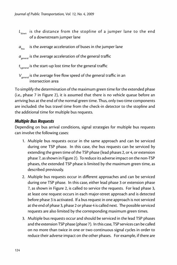
Journal of Public Transportation, Vol. 12, No. 4, 2009
124
Ldown is the distance from the stopline of a jumper lane to the end of a downstream jumper lane
abus is the average acceleration of buses in the jumper lane
ageneral is the average acceleration of the general traffic
tLgeneral is the start-up lost time for the general traffic
Vgeneral is the average free flow speed of the general traffic in an intersection area
To simplify the determination of the maximum green time for the extended phase (i.e., phase 7 in Figure 2), it is assumed that there is no vehicle queue before an arriving bus at the end of the normal green time. Thus, only two time components are included: the bus travel time from the check-in detector to the stopline and the additional time for multiple bus requests.
Multiple Bus RequestsDepending on bus arrival conditions, signal strategies for multiple bus requests can involve the following cases:
Multiple bus requests occur in the same approach and can be serviced 1. during one TSP phase. In this case, the bus requests can be serviced by extending the green time of the TSP phase (lead phases 2, or 4, or extension phase 7, as shown in Figure 2). To reduce its adverse impact on the non-TSP phases, the extended TSP phase is limited by the maximum green time, as described previously.
Multiple bus requests occur in different approaches and can be serviced 2. during one TSP phase. In this case, either lead phase 3 or extension phase 7, as shown in Figure 2, is called to service the requests. For lead phase 3, at least one request occurs in each major-street approach and is detected before phase 3 is activated. If a bus request in one approach is not serviced at the end of phase 3, phase 2 or phase 4 is called next. The possible serviced requests are also limited by the corresponding maximum green times.
Multiple bus requests occur and should be serviced in the lead TSP phases 3. and the extension TSP phase (phase 7). In this case, TSP services can be called on no more than twice in one or two continuous signal cycles in order to reduce their adverse impact on the other phases. For example, if there are
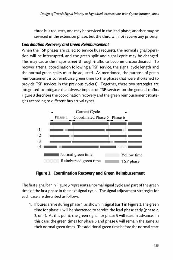
125
Design of Transit Signal Priority at Signalized Intersections with Queue Jumper Lanes
three bus requests, one may be serviced in the lead phase, another may be serviced in the extension phase, but the third will not receive any priority.
Coordination Recovery and Green ReimbursementWhen the TSP phases are called to service bus requests, the normal signal opera-tion will be interrupted, and the green split and signal cycle may be changed. This may cause the major-street through-traffic to become uncoordinated. To recover arterial coordination following a TSP service, the signal cycle length and the normal green splits must be adjusted. As mentioned, the purpose of green reimbursement is to reimburse green time to the phases that were shortened to provide TSP services in the previous cycle(s). Together, these two strategies are integrated to mitigate the adverse impact of TSP services on the general traffic. Figure 3 describes the coordination recovery and the green reimbursement strate-gies according to different bus arrival types.
Figure 3. Coordination Recovery and Green Reimbursement
The first signal bar in Figure 3 represents a normal signal cycle and part of the green time of the first phase in the next signal cycle. The signal adjustment strategies for each case are described as follows:
If buses arrive during phase 1, as shown in signal bar 1 in Figure 3, the green 1. time for phase 1 will be shortened to service the lead phase early (phase 2, 3, or 4). At this point, the green signal for phase 5 will start in advance. In this case, the green times for phase 5 and phase 6 will remain the same as their normal green times. The additional green time before the normal start

Journal of Public Transportation, Vol. 12, No. 4, 2009
126
point of the next signal cycle will be reimbursed to phase 1 in the following cycle. Thus, the next signal cycle can be recovered to the normal status.
If buses arrive at the end of phase 1 and have to take part of the normal green 2. time of phase 5, as shown in signal bar 2 in Figure 3, phase 5 will be terminated at the normal end point and the next phase will remain normal.
If buses arrive at the end of phase 5, the green time for phase 5 will be 3. extended (phase 7), as shown in signal bar 3 in Figure 3. The green time for phase 6 will be shortened to allow the next cycle to start on time.
If buses arrive during phase 6 of the previous signal cycle, this phase plus 4. phase 1 of the current cycle will be shortened to return the green signal to the lead phase early (phase 2, 3 or 4), as shown in signal bar 4 in Figure 3. The saved cycle time from phase 6 and phase 1 will be used to cover the lead phase(s), as well as the reimbursement time of phase 6 of the current cycle and phase 1 of the following cycle. This allows the next cycle to return to coordination. The reimbursed green time to phase 6 and phase 1 can be calculated individually by Equations (8) and (9) below:
where
greimb 6 is the reimbursed green time to phase 6
greimb 1 is the reimbursed green time to phase 1
∆gj is the loss of green time for phase j
glead is the green time for the lead phase
For multiple TSP services, which may occur in one cycle or two continuous 5. cycles, the saved cycle time will be cumulated and reimbursed in propor-tion to the green losses incurred by the corresponding phases using the following equation:

127
Design of Transit Signal Priority at Signalized Intersections with Queue Jumper Lanes
where
greimbj is the reimbursed green time to phase j
glead k is the green time for lead phase k
Simulation Implementation Because of the complex nature of traffic and human behaviors, TSP evaluation is increasingly relying on simulation tools (Dale 1999). VISSIM, a simulation tool known for its strengths in modeling transit operations, is selected for this study to simulate the different TSP design strategies with queue jumper lanes under dif-ferent traffic scenarios. Modeling TSP control strategies in VISSIM requires three main input files: (1) network configuration file *.inp, (2) TSP control logic file *.vap, and (3) phase and inter-phase definition file *.pua. The intersection simulated is assumed to have the same configuration, as shown in Figure 1. As shown, two bus stops are installed along the upstream jumper lane immediately behind the entry of the jumper lane, and there are three through lanes, one left-turn pocket, and one right-turn bay (jumper lane) for major-street approaches.
In this study, the performance of jumper TSP is compared with typical TSP appli-cations with mixed lanes. The same TSP strategies, including early green, green extension, coordination recovery, and green reimbursement, were applied to both jumper and mixed-lane TSP. The only difference was that the jumper phase (i.e., phase 2, 3, or 4) was applicable only to jumper TSP.
Because bus stop locations are known to have a major impact on bus opera-tion, the performance comparison also considers both near-side and far-side bus stops. The near-side bus stops were located along the jumper lanes for jumper TSP, as shown in Figure 1. These stops were installed immediately upstream of the check-in detectors to avoid impact on the TSP operations from bus dwell time variations. For mixed-lane TSP, the near-side bus stops are designed with bus bays and are located at the same locations as those of jumper TSP. The far-side bus stops for both mixed-lane TSP and jumper TSP were set along the same downstream right-turn pocket. Thus, in the case of mixed-lane TSP, the right-turn pocket serves as an extended bus bay. For jumper TSP with a far-side bus stop, no
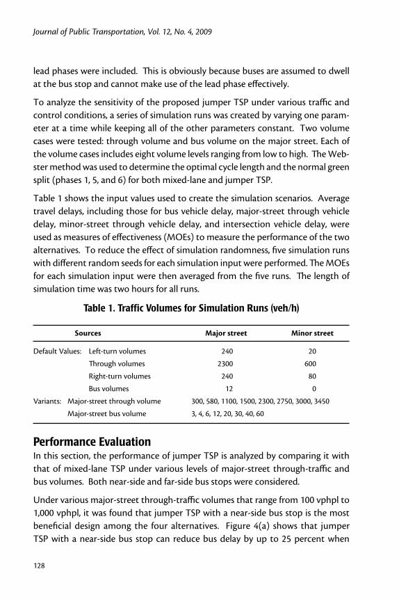
Journal of Public Transportation, Vol. 12, No. 4, 2009
128
lead phases were included. This is obviously because buses are assumed to dwell at the bus stop and cannot make use of the lead phase effectively.
To analyze the sensitivity of the proposed jumper TSP under various traffic and control conditions, a series of simulation runs was created by varying one param-eter at a time while keeping all of the other parameters constant. Two volume cases were tested: through volume and bus volume on the major street. Each of the volume cases includes eight volume levels ranging from low to high. The Web-ster method was used to determine the optimal cycle length and the normal green split (phases 1, 5, and 6) for both mixed-lane and jumper TSP.
Table 1 shows the input values used to create the simulation scenarios. Average travel delays, including those for bus vehicle delay, major-street through vehicle delay, minor-street through vehicle delay, and intersection vehicle delay, were used as measures of effectiveness (MOEs) to measure the performance of the two alternatives. To reduce the effect of simulation randomness, five simulation runs with different random seeds for each simulation input were performed. The MOEs for each simulation input were then averaged from the five runs. The length of simulation time was two hours for all runs.
Table 1. Traffic Volumes for Simulation Runs (veh/h)
Sources Major street Minor street
Default Values: Left-turn volumes 240 20
Through volumes 2300 600
Right-turn volumes 240 80
Bus volumes 12 0
Variants: Major-street through volume 300, 580, 1100, 1500, 2300, 2750, 3000, 3450
Major-street bus volume 3, 4, 6, 12, 20, 30, 40, 60
Performance EvaluationIn this section, the performance of jumper TSP is analyzed by comparing it with that of mixed-lane TSP under various levels of major-street through-traffic and bus volumes. Both near-side and far-side bus stops were considered.
Under various major-street through-traffic volumes that range from 100 vphpl to 1,000 vphpl, it was found that jumper TSP with a near-side bus stop is the most beneficial design among the four alternatives. Figure 4(a) shows that jumper TSP with a near-side bus stop can reduce bus delay by up to 25 percent when
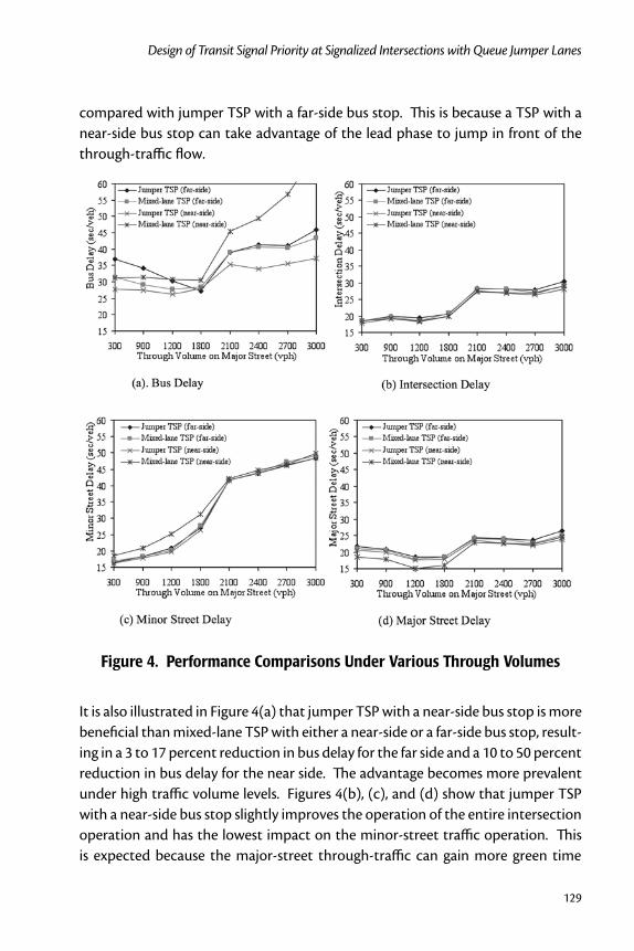
129
Design of Transit Signal Priority at Signalized Intersections with Queue Jumper Lanes
compared with jumper TSP with a far-side bus stop. This is because a TSP with a near-side bus stop can take advantage of the lead phase to jump in front of the through-traffic flow.
Figure 4. Performance Comparisons Under Various Through Volumes
It is also illustrated in Figure 4(a) that jumper TSP with a near-side bus stop is more beneficial than mixed-lane TSP with either a near-side or a far-side bus stop, result-ing in a 3 to 17 percent reduction in bus delay for the far side and a 10 to 50 percent reduction in bus delay for the near side. The advantage becomes more prevalent under high traffic volume levels. Figures 4(b), (c), and (d) show that jumper TSP with a near-side bus stop slightly improves the operation of the entire intersection operation and has the lowest impact on the minor-street traffic operation. This is expected because the major-street through-traffic can gain more green time
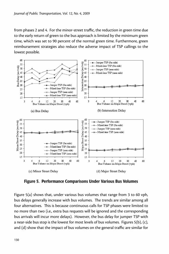
Journal of Public Transportation, Vol. 12, No. 4, 2009
130
from phases 2 and 4. For the minor-street traffic, the reduction in green time due to the early return of green to the bus approach is limited by the minimum green time, which was set to 90 percent of the normal green time. Furthermore, green reimbursement strategies also reduce the adverse impact of TSP callings to the lowest possible.
Figure 5. Performance Comparisons Under Various Bus Volumes
Figure 5(a) shows that, under various bus volumes that range from 3 to 60 vph, bus delays generally increase with bus volumes. The trends are similar among all four alternatives. This is because continuous calls for TSP phases were limited to no more than two (i.e., extra bus requests will be ignored and the corresponding bus arrivals will incur more delays). However, the bus delay for jumper TSP with a near-side bus stop is the lowest for most levels of bus volumes. Figures 5(b), (c), and (d) show that the impact of bus volumes on the general traffic are similar for
131
Design of Transit Signal Priority at Signalized Intersections with Queue Jumper Lanes
all four alternative TSP designs. This is expected as the general bus frequencies do not significantly affect the traffic load on the same approach.
ConclusionsIn this study, an effective design of TSP with queue jumper lanes has been proposed, including special phase design, signal timing parameter determination, coordina-tion recovery and green reimbursement strategies, and a strategy for multiple bus requests for priority service. The performance of the proposed jumper TSP was evaluated in a micro-simulation environment by comparing its performance with that of the general mixed-lane TSP under various traffic volumes and bus stop locations. The simulation results demonstrated that jumper TSP with a near-side bus stop and a consequent reduction of bus delay up to 25 percent is superior to its far-side counterpart. The simulation results also showed that jumper TSP with a near-side bus stop can reduce bus delay by 3 to 17 percent when compared with mixed-lane TSP with a far-side bus stop, which was the most commonly-used TSP design. The advantages become more prevalent in situations involving high traf-fic volumes. The simulation results also showed that major-street general traffic can also benefit from jumper TSP phases and the adverse impact on minor-street general traffic can be reduced to a negligible level through proper coordination recovery and reimbursement strategies. It was also shown that the impact of bus volumes on the general traffic on both major and minor streets is not significantly different from the mixed-lane TSP. This is achieved by limiting the continuous calls for TSP to no more than two.
References
Balke, K. N., C. L. Dudek, and T. Urbanik. 2000. Development and evaluation of intelligent bus priority concept, Transportation Research Record 1727: 12-19.
Dale, J., T. Bauer, R. Atherly, and L. Madsen. 1999. A transit signal priority impact assessment methodology: Greater reliance on simulation, Proceedings of the 78th Annual Meeting of the Transportation Research Board, Washington, DC.
Head, K. L. 1998. Improved traffic signal priority ror Transit, TCRP Project A-16, Interim Report.
Liu, H, A. Skabardonis, W. Zhang; M, Li. 2004. Optimal detector location for bus signal priority, Transportation Research Record 1867: 144-150.

Journal of Public Transportation, Vol. 12, No. 4, 2009
132
Nowline, L. and K. Fitzpztrick. 1997. Performance of queue jumper, Proceedings of Traffic Congestion and Traffic Safety in the 21st Century: Challenges, Innova-tions, and Opportunities, Chicago, IL.
Zhou, G. W. and A. Gan. 2005. Performance of transit signal priority with queue jumper lanes, Transportation Research Record 1925: 265-271.
Zhou, G.W. and A. Gan. 2006. Optimal detector locations for transit signal priority with queue jumper lanes, Transportation Research Record 1978: 123-129.
About the Authors
Guangwei Zhou ([email protected]) is an ITS Engineer with HDR Engineer-ing Inc. He graduated from Florida International University with a Ph.D. in 2006. His interest areas include Intelligent Transportation Systems (ITS) planning and design, transit operations analysis, traffic modeling and simulation, and traffic design.
Albert Gan ([email protected]) is an Associate Professor with the Department of Civil and Environmental Engineering at Florida International University. He received his Ph.D. in Civil Engineering from the University of Florida in 1996. His areas of research have included traffic simulation, intelligent transportation systems (ITS), transit planning, demand modeling, and highway safety.