NBER WORKING PAPER SERIES

PUBLIC MONOPOLY AND ECONOMIC EFFICIENCY:EVIDENCE FROM THE PENNSYLVANIA LIQUOR CONTROL BOARD'S ENTRY DECISIONS

Katja SeimJoel Waldfogel

Working Paper 16258http://www.nber.org/papers/w16258

NATIONAL BUREAU OF ECONOMIC RESEARCH1050 Massachusetts Avenue

Cambridge, MA 02138August 2010

We thank seminar participants at Kellogg, MIT, Ohio State, Texas, Toronto, Virginia, Wisconsin,the Tenth CEPR Conference on Applied Industrial Organization, and the 2010 NBER Winter IO Meetingsat Stanford. We are grateful to Tim Bresnahan for comments on an earlier draft. We thank ThomasKrantz at the Pennsylvania Liquor Control Board for helping us to get access to the data. All errorsare our own. The views expressed herein are those of the authors and do not necessarily reflect theviews of the National Bureau of Economic Research.

NBER working papers are circulated for discussion and comment purposes. They have not been peer-reviewed or been subject to the review by the NBER Board of Directors that accompanies officialNBER publications.

© 2010 by Katja Seim and Joel Waldfogel. All rights reserved. Short sections of text, not to exceedtwo paragraphs, may be quoted without explicit permission provided that full credit, including © notice,is given to the source.

Public Monopoly and Economic Efficiency: Evidence from the Pennsylvania Liquor ControlBoard’s Entry DecisionsKatja Seim and Joel WaldfogelNBER Working Paper No. 16258August 2010JEL No. L13,L21,L3,L81

ABSTRACT

While private monopolists are generally assumed to maximize profits, the goals of public enterprisesare less well known. Using the example of Pennsylvania’s state liquor retailing monopoly, we useinformation on store location choices, prices, wholesale costs, and sales to uncover the goals implicitin its entry decisions. Does it seek to maximize profits or welfare? We estimate a spatial model ofdemand for liquor that allows us to calculate counterfactual configurations of stores that maximizeprofit and welfare. We find that welfare maximizing networks have roughly twice as many stores aswould maximize profit. Moreover, the actual network is much more similar in size and configurationto the welfare maximizing configuration. An alternative to a state monopoly would be the commonpractice of regulated private entry. While such regimes can give rise to inefficient location decisions,little is known about the size of the resulting inefficiencies. Even for a given number of stores, a simplecharacterization of free entry with our model results in a store configuration that produces welfarelosses of between 3 and 9% of revenue. This is a third to half of the overall loss from unregulatedfree entry.

Katja SeimThe Wharton SchoolUniversity of Pennsylvania3620 Locust WalkPhiladelphia, PA 19104-6372kseim@wharton.upenn.edu

Joel WaldfogelFrederick R. Kappel Chair in Applied Economics3-177 Carlson School of ManagementUniversity of Minnesota321 19th Avenue SouthMinneapolis, MN 55455and NBERjwaldfog@umn.edu

1

I. Introduction Governments operate a substantial number of enterprises around the world, sometimes

with legal monopolies. In addition to familiar examples such as roads, public transport, and utilities, various levels of government in the U.S. also provide mail delivery services and operate municipal libraries, hospitals, elementary and secondary schools, and retail stores in products such as liquor.1 Examples of public enterprise are plentiful outside of the U.S. as well and include airlines, telecommunication services, and retail banking services. One such government monopoly is the retail liquor business in Pennsylvania. The Pennsylvania Liquor Control Board (PLCB) has the exclusive right to operate liquor (“wine and spirits”) shops in the Commonwealth of Pennsylvania, and it operates over 600 stores throughout the state. Prices are set by the state legislature via markup rules, but the PLCB controls entry; it has the authority to choose the number of stores it operates as well as where to locate them.

It is customary to assume that a private monopolist would choose a store configuration to maximize its profits, and economic theory provides clear guidance on how to do this. But what goals do public enterprises pursue through their managerial decisions?2 The operation of the PLCB provides some evidence on this question. Using Pennsylvania data, we ask what goal the PLCB pursues through its store location decisions. Does it seek to maximize profits? Or does the state’s planner take account of consumers as well as producers in determining its configuration? To study these questions we develop a simple model of demand for a product located in geographic space. In our model – as in the empirical context that we study – prices are fixed. Consumers are distributed across the state, and they benefit, in the form of lower effective prices, from proximity to outlets. Additional outlets, however, are costly to run. The state’s problem is to choose a set of store locations – and a corresponding number of stores operating – to best serve its objective. Given the state’s choice of locations for stores, our goal is to compare the actual configuration to the two theoretical benchmarks of profit and welfare maximization.

We estimate a model of demand for liquor as a function of the price, distance to stores, and other demographic characteristics. The price elasticity and the disutility from travel are the two key parameters that together allow us to quantify the consumer benefit from greater proximity. We observe the fixed retail price as well as the wholesale cost, allowing direct calculation of producer surplus. The model allows us to calculate demand, consumer surplus, and producer surplus for any configuration of stores. In particular, we calculate configurations of stores that maximize profit as well as configurations that maximize total welfare. We then

1 See, for example, Boardman and Vining (1989) for a prominent study comparing the efficiency of private and public enterprises. Glaeser (2001) provides a discussion of public enterprises in cities. 2 There is a literature on public sector pricing (See Bös (1985)). We instead focus on a public enterprise’s entry decisions.

2

compare the actual PLCB store network to these analogs of theoretical benchmarks. We find that welfare maximizing networks have roughly twice as many stores as would maximize profit. Moreover, the actual network is much more similar in size and configuration to the welfare maximizing configuration. We conclude that the state’s behavior is better described by welfare than by profit maximization.

We then turn to simulating alternative policies for controlling the size of the store network. In the absence of a state monopoly, Pennsylvania might follow most other states with regulated private entry. In most places around the U.S., jurisdictions regulate the maximum number of liquor stores using transferrable licenses, and independent private agents choose where to locate them within each jurisdiction. It is well known in theory – since Hotelling (1929) – that free entry in differentiated product markets can give rise to inefficient location decisions, but the magnitude of the resulting inefficiencies are unknown. We use our model – and an implementable notion of private entry – to explore the properties of regulated private entry. Not surprisingly, unregulated entry generates welfare losses relative to the welfare maximizing configuration of 10 to 15% of welfare maximizing revenue due to both incorrect numbers of entrants and suboptimal location choices. But even for a given number of stores, unregulated entry results in welfare losses from excessive clustering of stores around high-demand areas of between 3 and 9% of revenue in the contexts we analyze, a third to half of the overall loss. Of course, these losses must be balanced against other possible effects of private entry beyond what we model, such as price changes and reductions in the cost of operating stores.

Our paper proceeds in eight sections. First, section 2 presents a simple theoretical model that illustrates the differing theoretical benchmarks of profit-maximization, welfare-maximization, and competition. We then proceed to a description of the PA liquor retailing system, current policy discussions, and a discussion of the data used in the study. Section 3 describes the data and documents the relationships of interest for the study. Section 4 presents estimates of a simple model of liquor demand at particular stores. We then turn to exercises made possible by the model. Section 5 evaluates the system based on the incremental benefits of existing stores and infers the implicit welfare weights that PLCB entry decisions attach to various types of consumers. Section 6 presents simulation results based on profit and welfare maximization for five counties of varying sizes: (i) we derive the optimal geographic configuration of stores for profit and welfare maximization; (ii) and we develop a tractable algorithm for calculating optimal configurations in larger areas, and we show that it approximates the exact solution well for the counties. Section 7 turns to the statewide problem and uses the simple algorithm to determine profit and welfare-maximizing configurations for the

3

whole state. Section 8 then analyzes the welfare properties of regulated but atomistic private entry. We first present an approach to determining approximate free entry equilibria in small (and medium-sized) pieces of geography. We then run this algorithm on our five counties in Pennsylvania. We calculate the number of stores operating under free entry as well under regulated private entry to target the actual number of stores operating.

II. A Model Illustrating Rationales for Entry Patterns

Consider the following simple model with fixed prices and transport costs. Consumers are uniform on [0, 100]. The price of the product is $10. Marginal costs are $0, and fixed costs are $240. Consumers derive 60 .

Assume temporarily that firms choose equidistant locations. Provided at least one firm operates and chooses its profit maximizing location, all 100 consumers buy since 0 throughout the space. With outlets spaced symmetrically at 2 , 0,…, 1 and

, consumer surplus can then be expressed as a function of the distance traveled by consumers at the midpoint between two stores, :

100 60 10 . (1)

If one firm operates, it will garner the most business locating at 50. Because U > 0 throughout the space when the store locates at 50, all 100 consumers buy, so revenue is $1,000 (and profits are $760). Consumer surplus is 2,500. If more firms operate, all consumers will continue to buy, so revenue and producer surplus remain $1,000, although profits fall by the fixed cost with each entrant. Consumer surplus rises even though prices are fixed because stores get closer to consumers who therefore incur smaller travel costs. That profits fall with entry while consumer surplus rises creates the tension between the interests of consumers and producers.

In this setup, a monopolist maximizing profits would choose a single store ( 1). A welfare maximizing planner, by contrast, chooses 3. Free entry dissipates the entire producer surplus (up to an integer constraint) and results in 4 firms operating.3

While simple, this model shows important consequences of different firm goals and ownership arrangements. A monopolist seeking to maximize profits would operate too few outlets. Free entry, on the other hand, would result in too many. Equi-distantly spaced location

3 This simple model does not allow additional stores to raise revenue, but welfare maximization yields more entry than monopoly in more general models. See Spence (1976), Dixit & Stiglitz (1977), and Mankiw and Whinston (1986).

4

choices are typically not sustainable in equilibrium; hence free entry also has the potential for generating losses from firms choosing the wrong locations in addition to the welfare losses from the wrong number of firms. For example, the well-known Hotelling duopolists cluster at the center of the space under free entry even though welfare maximization dictates spreading. The Hotelling result is fragile, and it is in general difficult to analytically predict effects of ownership structure on product mix. With three stores or more, the model has no pure strategy Nash equilibrium when consumers patronize their nearest store (de Palma, Ginsburgh, and Thisse (1987)). We consider similar benchmarks for comparison with the PLCB’s entry decisions below.4

III. Background and Data

Background

Pennsylvania is the largest of 18 “control” states that control the sale and distribution of alcohol at the wholesale and retail levels in different forms. The states take different approaches to liquor retailing, however. Some states employ regulated private entry, allowing fully private retailing operations but limiting the supply of licenses, generally within each municipality; others turn over the operation of state stores to private enterprises; yet others continue to operate state-run stores that in some cases compete with privately-run stores. Pennsylvania operates a privatized system for the sale of beer, but acts as a state monopolist in the wholesale and retail distribution of wine and liquor through a system of state-run stores.

As of the first week of 2005, the state operated 624 stores. We can calculate each store’s ambient demographics, based on Census tracts for which the store is closest. By this method, for the first week of the year, the average ambient population of a store was 18,154. The inter-quartile range ran from 12,842 to 24,781. Assuming that all population resides at Census tract centroids, the average (median) great-circle distance to the nearest store was 3.2 (2.4) kilometers, with an interquartile range of 1.0 to 3.6 km.

While privatization is not currently under discussion, the PLCB has taken strides toward improving the system’s efficiency and consumer friendliness. In the 1970s the stores consisted of a front counter where a customer would request a bottle of liquor from the back room. In the last few years the stores have added chilled rooms for fine wines in many stores. According to an August 2007 press release, the agency has recently tried to operate more “like a business” and hired a CEO to oversee day to day operations: “Governor Rendell has given this agency a

4 A number of studies examine the positive effects of ownership structure – and internalization of business stealing – on product spreading. See Steiner (1952), Berry and Waldfogel (2001), and Sweeting (2009).

5

mandate to operate like a business, and that means getting costs under control.” One strategy the PLCB has recently pursued is reducing the number of stores operating. According to PLCB Chairman Patrick Stapleton, “We took important steps last year toward that end, starting with reducing the number of stores in our system to 630 from 646 a year earlier. This year, PLCB 75 [the Board’s strategic plan] will continue to make improvements to our operations that will have a direct impact on our bottom line, and in how Pennsylvanians interact with us.”5

External observers agree that store closings are an avenue to greater profitability for the system. A private equity lawyer quoted in the Pittsburgh Gazette speculated that private owners would achieve greater profitability by closing stores in remote locations rather than by replacing union workers with minimum wage clerks. At the same time, the Independent State Store Union criticized the PLCB for being too focused on profit in reducing the number of stores, suggesting that small, rural communities are hurt in availability from a move toward profit maximization.6 There is also speculation in the press that political lobbying and considerations play a significant role in store closing, countering the stated profit motives of the board.7

In 2005 and 2006, the PLCB opened a small number of outlets within the premises of grocery stores. The PLCB further operates seven “outlet” stores near the borders with neighboring states.8 As of the first week of 2005, 65 stores, or 10.37%, are designated premium-collection stores that are larger in size and carry a wider variety of products than the remaining locations. Lastly, approximately 25% of stores are open part of the day on Sunday. While most of the remaining stores are open 6 days per week, 56 stores are closed on two or more days per week. 17 additional stores were closed for part of some (random) weeks in 2005, presumably for repairs etc. These asynchronous closures provide useful variation for identifying the relationship between store proximity and purchase behavior.

The PLCB charges an identical retail price for a particular product in all of its stores and uses a simple mark-up rule to determine the price, applying a 30% markup and an 18% liquor tax to the wholesale price.9 The PLCB engages in some promotional activity, using manufacturers’

5 PA LIQUOR CONTROL BOARD REPORTS RECORD RETURN FOR FISCAL 2006-07, August 28, 2007. Press release. http://www.lcb.state.pa.us/webapp/agency/press/press_detail.asp?press_no=07-18&psearch=&offset=4, accessed October 17, 2008. 6 Pittsburgh Post Gazette, “Is Time Right to Sell State Stores?” June 12, 2007. http://www.post-gazette.com/pg/07163/793365-85.stm, accessed October 17, 2008. 7 Pittsburgh Post Gazette, “LCB works in curious ways” January 1, 2008. http://www.post-gazette.com/pg/08028/852743-85.stm, accessed October 17, 2008. 8 In addition to the typical selection, the PLCB sells certain products at outlet stores that are unavailable in the remaining stores. These tend to be larger-sized bottles or multi-packs. 9 The specific pricing rule is: 1.3 1.18 , where the bottle fee amounts typically to $1 and the PLCB rounds the resulting retail price to end in the nearest nine cents. In addition, the consumer pays a 6% PA sales tax.

6

coupons and running system-wide monthly sales (28-day period beginning on the Monday closest to the end of the month).

The PLCB negotiates wholesale prices directly with its suppliers. A new product’s wholesale price remains fixed for one year after introduction. For established products, the PLCB re-negotiates over cost increases on a quarterly basis rotating through product categories over the course of its four-week long reporting periods. Each reporting period, the wholesale price of a subset of products is adjusted, translating into changes in the retail price. In contrast to sales periods, reporting periods begin on a Thursday, usually in the middle of the month. Prices can therefore change at two discrete times per month.10

We consider as fixed costs the PLCB’s cost to run stores (personnel, rental cost of property, storage, etc.) and warehousing. We do not observe store-level fixed costs directly, but we know that system-wide, the PLCB used $245.9 million to run stores and warehousing in fiscal year 2004-‘05. This corresponds to $394,051 per store in annual fixed costs (or $1,110 per day), given 624 stores in operation as of 1/2005.11

Data

The basic data set for the study is a store-level panel obtained from the PLCB under the Pennsylvania Right-to-Know Law.12 It contains daily information on quantities sold and gross receipts at the product and store level during 2005. In addition, we received information on the wholesale cost of each product that is constant across stores and varies over time according to the reporting periods described above. We geocode the stores’ street addresses to assign them to a geographic location, which we link to data on population and demographic characteristics for nearby consumers based on information from the 2000 Census and Reference USA. Because stores open and close during the year, the characteristics of stores’ ambient consumers change over time.

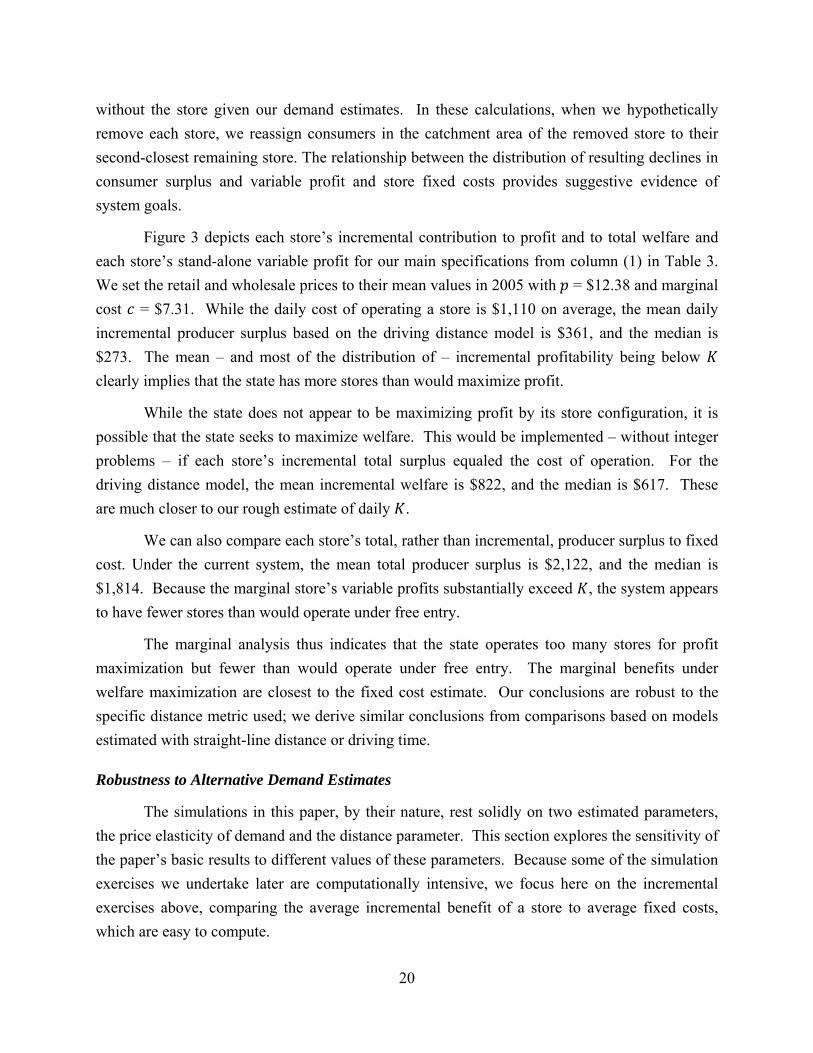
We aggregate our data across products to the level of either the day or the week. This periodicity accounts for the strong seasonality inherent in liquor sales, which are disguised in more aggregate definitions. Averaging across 32,509 store weeks in 2005, stores sell an average of 2,674 bottles per week. Figure 1 exhibits the strong seasonal pattern to sales, with a trough after New Years (week 1) and peaks at July Fourth (week 26), Thanksgiving (47), and Christmas through New Year’s Eve (50-52). 10 In our data below, 90.26% of price changes occur within one week from the beginning of a new reporting or sales period, reflecting that not all products have daily sales in at least one PLCB store. 11 PLCB’s fiscal year 04-05 summary, http://www.lcb.state.pa.us/plcb/cwp/view.asp?a=1334&q=557420&tx=1, accessed 11/5/2008. 12 65 P.S. §§ 66.1 et seq., as amended.

7

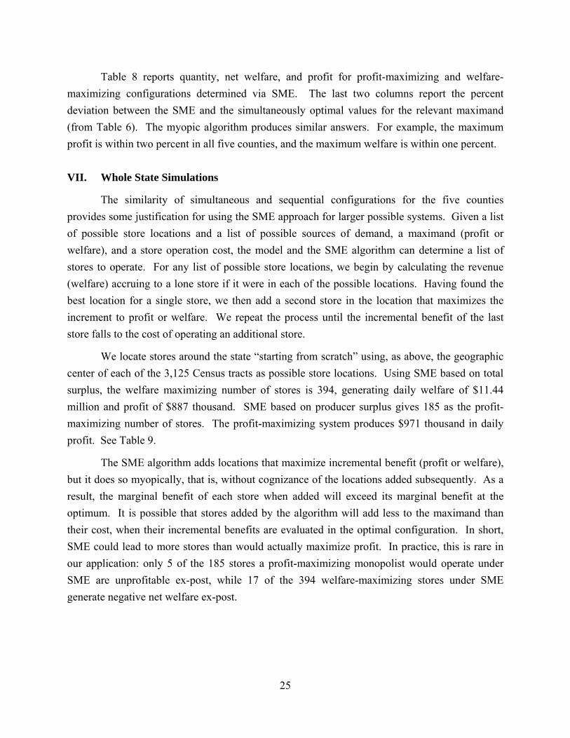
Because we treat liquor as a single quantity in our analysis below, we also need a single price. PLCB stores carry literally thousands of products, and we calculate a state-wide price index, shown in Figure 2, that is a weighted sum of the system-wide product prices in each week. We use fixed weights – the products’ shares of 2005 sales – to avoid contaminating the price index with quantity responses. The resulting price series resembles a step function, reflecting the discrete changes in prices due to either sales or wholesale cost changes discussed above.

While stores differ in the product composition of purchases, these differences reflect heterogeneity in consumer preferences more than differences in the availability of products across stores. Absent inventory information at the store and product level, we can derive product availability from observed purchases only and treat a product as being available in a store if it sold at least once during a given week. Of the 100 best selling products statewide in 2005, the median store carried 98.0% in its median week, while a store at the fifth percentile carried 72.0% of the products. Similarly, of the 1000 best selling products statewide in 2005, the median store carried 82.03% in its median week, while a store at the fifth percentile carried 44.2% of the products. The product availability at premium stores is somewhat better than the average, with the median premium store carrying all of the top 100 products and 95.1% of the top 1000 products. But most stores carry most products, supporting our assumption below that differences in product availability do not drive customers’ store choices to a significant degree. In our empirical exercises below we employ a single statewide price index reflecting our model’s implicit assumption of a single identical product available at each store.13

Descriptive Evidence

Our model of demand will link purchase behavior to demographic characteristics, the configuration of stores, and price. In this section we explore these relationships as a step toward more formal estimation. We first examine the relationship between prices and demand, via regressions of log quantities on measures of log prices as well as flexible time effects. Our price measures vary only across time and not place, in line with the PLCB’s uniform pricing policy, and thus do not allow fully flexible time dummies. It is possible that prices move endogenously with anticipated changes in demand. We address this potential endogeneity of the price series in a number of ways.

First, we employ a price index that removes price declines due to potentially endogenous sales. We call this the list price and build a statewide, fixed weight, price index based on it. The first two columns of Table 1 report the results of log-log regression of weekly quantity on the

13 We performed various descriptive exercises (like those in Table 2 below) with store-specific price indices, and their use gives rise to demand elasticities similar to those implied by the statewide index.

8

state-bundle list price index with selected holiday week dummies and, in column (2), store fixed effects. This results in a price elasticity of approximately –1. Columns (3) and (4) repeat this exercise with a more flexible quadratic seasonality specification, allowing seasonal effects to differ in the last six weeks of the year from the trend of the earlier months. Because we include flexible week dummies, the price elasticity is identified from the co-variation in quantity and the price index after accounting for the constant-across-store change in sales experienced at the same time. This approach yields an elasticity of –1.3.

Second, we use a price index based on the actual price series, which reflects price reductions due to sales. We control for unusual spikes or declines in demand around holidays by including time dummies for holiday weeks or days. These time effects address endogeneity concerns to the extent that they control for the relevant temporary changes in demand that the PLCB anticipates in choosing its sale prices. Repeating the exercises of columns (1) through (4) using the actual price gives a similar range of price elasticity estimates, from –0.9 to –1.9, in columns (5) through (8). Columns (9) and (10) use the actual price with daily data, allowing finer controls for seasonality, giving elasticity estimates of –0.6 and –0.7.

Last, we limit our sample to days immediately prior to and immediately following price changes. If the PLCB chooses sales in response to other anticipated non-holiday demand spikes in addition to the ones we control for, the price elasticities in columns (5) through (10) would still be biased. The immediate response in sales to a price change provides clean identification provided the underlying demand does not change significantly between the day before and the day of a price change and provided that customers do not anticipate the sale. Columns (11) and (12) depict estimated elasticities for this subsample of the daily data (–0.7 and –1.2), again in line with the results above.

Table 1 thus indicates that demand for liquor is higher when the price is lower, with a price elasticity between –0.6 and –1.9. This is in line with estimates from the large empirical literature attempting to measure the elasticity of demand for liquor. Cook and Moore (1999) review the literature on demand for alcohol, most of which use state-level time series data. According to Chaloupka, Grossman, and Safer (2002), “An extensive review of the economic literature on alcohol demand concluded that based on studies using aggregate data (i.e., data that report the amount of alcohol consumed by large groups of people), the price elasticities of demand for beer, wine, and distilled spirits are –0.3, –1.0, and –1.5, respectively (Leung and Phelps 1993).”

The second relationship of interest is between ambient population and quantity demanded. Table 2 explores this relationship systematically with multiple regression. The first

9

column reports a regression of average weekly bottles on ambient population and the distance to nearby stores, using the cross section of stores operating in the first week of the year. The population coefficient is positive: each additional 1000 people nearby add 17 bottles per day. The farther people live from the store, the lower is demand. Column (2) repeats the exercise using log sales as the dependent variable. Using the daily data gives us temporal price variation, and when the list price is included in column (3), population increases demand while distance decreases it, and the elasticity of demand with respect to the statewide bundle price is –0.9.

Given that we have multiple observations on quantity and demographic characteristics for each store, fixed effects seem a natural approach to deal with unobserved spatial heterogeneity. Ideally, if we had, say, tract level data on demand, then tract fixed effects would allow us to estimate the distance parameter cleanly using only the variation in demand between days when the distance to the nearest store changes. However, we do not observe the demand associated with particular consumers. Instead, we observe store-level demand. Because the group of consumers nearest each store varies across days, a store fixed effect does not control for the same consumers’ unobserved demand. Hence, the usual argument why fixed effects provide an estimate purged of unobserved heterogeneity is not correct in this context. Nevertheless, we provide estimates with store fixed effects to see what suggestive descriptive relationships the data contain. With store fixed effects and the statewide bundle price (in columns (3) and (4)), the population and distance coefficients both decline in absolute magnitude, but their signs remain consistent with earlier estimates. Columns (5) and (6) revisit the analyses of (3) and (4) using the actual price, with similar results.

Since our data are at the store, rather than the consumer, level, we cannot directly explore the extent to which people who live further from a store choose to make fewer, but larger, shopping trips and store the product more. However, we do not observe a larger response to a price decline for stores that serve a more distant population. In regressions of the absolute or percentage change in daily sales on the day (or days) following a price decline, stores with a higher average distance to consumers experience a lower, generally statistically insignificant, increase in sales due to the drop in prices, conditioning on the amount of the price change and other demographics of the catchment area. If storage were important, we would expect a larger response with consumers in more distant areas stocking up more intensively.

We also explored descriptively how sensitive the results in Table 2 are to some of the salient features of the Pennsylvania liquor market. First, we re-estimated specifications (3) and (4) excluding holiday weeks (Thanksgiving week and last three weeks of December) from the sample, to test whether the base results are driven by differences in willingness to pay for liquor or travel to the store in these unusual weeks. We obtained very similar results with this limited

10

sample. Second, we explored whether systematic differences in demand in areas close to Pennsylvania’s borders, including in Philadelphia and Pittsburgh, drive the relationships in Table 2. Demand in these areas may be more elastic than in the interior of the state due to the easier access to alternative shopping sources. The descriptive regressions did not yield conclusive evidence to that effect.

Table 1 and Table 2 provide clear evidence for the mechanisms that underlie our story: having more potential customers nearby raises demand, as does their proximity to their nearest store. Higher prices reduce demand, via the demand curve. We now turn to a simple model to estimate these effects, while allowing us to predict sales under alternative store configurations.

IV. A Simple Model of Demand with Travel Cost

We seek a model that, for any set of store locations, can indicate both the demand and producer and consumer surplus from consumption by individuals in each piece of geography. The key behavioral relationships that the model must describe are a) the sensitivity of demand to consumers’ distance to stores and b) the price elasticity of demand, which allows us to attach a dollar value to proximity. We could directly relate quantities sold at a store to, say, population in its area and other demand shifters, such as the percent black or median income in the area. Table 2 reports such regressions, but they cannot be used to predict sales under a counterfactual set of stores or locations and, in turn, to calculate the change in consumer surplus from an additional store or a change in store configuration. This goal, instead, requires a model of demand at the level of geography where consumers reside. We use a discrete-choice framework to model the consumer’s decision to purchase liquor and estimate its parameters based on the PLCB’s current stores to address these requirements.

Demand and Distance

There are stores located around the state. We assume that a consumer patronizes the store nearest his residence. This assumption, which would arise endogenously if stores were identical in selection, given that pricing is identical across stores, divides the state into catchment areas containing all of the population nearest to each store. We make this assumption, as well as several others, to facilitate the determination of optimal store configurations using integer programming, discussed below.

We denote each store’s catchment area by . Formally, is the set of consumer locations such that store location is the closest to location on day , or :min 1, … , , 1, … , , where denotes the distance, measured in an appropriate metric, of consumer in location from the store’s location . Since in our data, we

11

observe a single store per location, we denote both the store and its location by . Due to permanent store closures and openings and variation in store openings over the course of the week, catchment areas vary over time.

We discretize consumer locations in the state by modeling demand at the level of the Census tract and place all resident at each tract’s centroid. We then assign Census tracts to store catchment areas by finding the store that is closest in distance to each tract centroid. While the use of Census tracts – relative to finer divisions of the state such as Census block groups – introduces some measurement error into the distances consumers travel, it yields a more manageable set of 3,125 potential store locations for the simulations that follow.

Our lack of data on individual purchases does not allow us to distinguish between the decision to visit a store and the decision of how many bottles to purchase. Instead, we assume that consumers purchase a single bottle of liquor during a shopping occasion and model consumer ’s conditional indirect utility from traveling to store on day to purchase a bottle of liquor as: . (2)

We aggregate consumers to demographic groups , differentiating between black ( ) and other-race residents ( ). In equation (2), is a vector of attributes for consumers of type in location and seasonal effects. denote unobserved utility shifters that we assume to be distributed extreme value.

A consumer chooses to purchase from his store provided that his utility exceeds the utility of the outside option of not purchasing. We normalize its value to zero. Our assumption of extreme-value distributed yields Logit purchase probabilities for consumers of each demographic group in a particular location :

. (3)

To derive a store’s predicted demand, we aggregate over the decisions of potential consumers across demographic groups within a tract location and across all of the locations that make up a store catchment area, . We consider as potential consumers the population of each Census tract over the age of 21. Aggregate demand for liquor in tract , , and at store , , is thus the weighted average probability of purchase across demographic types and, for the store, across tracts, using as weights each tract’s mass of consumers of a particular type, scaled up by the total potential consumers:

12

∑ , , |β,

∑ , (4)

where denotes the number of potential consumers of type in tract location and ∑ ∑ , the potential consumers in the store’s aggregate catchment area.

Estimation proceeds via maximum likelihood. The parameter estimates maximize the likelihood of observing actual sales in store on day , , given data on the price of liquor and on the demographics and distance from the store of the locations making up the store catchment area. The log-likelihood function is given by:

ln ∑ ∑ ln ln 1 , (5)

where is an indicator of whether store is open on day . We identify the parameters from observing variation in the price of liquor over time ( and cross-sectional and time-series variation in the composition of catchment areas, resulting in variation in distances traveled ( and demographic attributes .

Demand Model Estimates

To keep the data manageable, we rely on a randomly drawn 10% subset of the daily data.14 We allow each demographic group’s utility function to have its own intercept that shifts with the group’s per-capita income and median age using data from the Census 2000. We further include in utility each tract’s number of churches per-capita, derived from a state-wide listing of religious organizations (NAICS 81311008) from Reference USA, to proxy for variation in local attitudes toward liquor consumption.

As in our descriptive regressions, we address the fact that the PLCB may time sales and thus price reductions to coincide with unobserved temporal variation in liquor demand by employing the list-price prior to sales as our price index for the composite liquor product. We also control for seasonal effects flexibly by including day of the week effects, week dummies for holiday weeks (the week after New Years (week 1), July Fourth (week 26), Thanksgiving (47), and Christmas through New Year’s Eve (50-52)), and additional holiday dummies for Memorial Day (May 28, 2005), days close to July 4 (June 30, July 1 – July 3), Labor Day (September 3, 2005), and days around Thanksgiving (November 23 – 26). The price elasticity is thus identified from a response in sales to price changes in otherwise similar days.

14 For the descriptive regressions in Table 2, the estimated parameters using the subsample do not differ significantly from the results obtained using the full sample of data.

13

Lastly, we consider three different distance-based proxies for travel cost. We employ the great-circle distance in kilometers between locations. A more realistic proxy for the consumer’s travel cost consists of the distance traveled along the existing road network. We compute the distances based on the shortest route between two locations, using the program MPMileage. We do so for the distances between all PA Census tracts and the existing stores, as well as – for the purposes of computing demand under counterfactual store configurations below – between all PA Census tracts and the 25 tracts closest to each tract based on great-circle distance. MPMileage further generates the average travel time in minutes between any two locations, which we use as our last travel cost proxy, to capture differences between urban, suburban, and rural locations in congestion and in the types of roads used to travel to the store.

Driving distance (and time) is, not surprisingly, systematically larger than, but closely related to, great-circle distance. A regression of driving distance to the closest store on great-circle distance to the closest store for each of Pennsylvania’s 3,125 tracts indicates that each additional kilometer of great-circle distance adds 1.4 km of driving distance, with an R2 of 0.94. The regression also indicates that, on top of the aspect of driving distance that is proportional to great-circle distance, driving distance contains an additional 0.2 km, or systematic deviations from proportionality. These deviations from proportionality leave room for possible differences in the estimated demand models using the alternative distance measures.

The coefficients of the estimated demand function appear in Table 3. Column (1) reports results based on driving distance in km as our distance metric. These are the results we rely on in the remainder of the paper. Columns (2) and (3) report the results based on great-circle distance and driving time in minutes, respectively. Most of the parameters are stable across specifications. The estimated price coefficients translate into an average price elasticity of –1.18 to –1.28, similar to the estimates in Table 1 and Table 2.

In specification (1), the estimated distance parameter of –0.066 indicates that demand declines by 40 cents (64 cents) for every kilometer (mile) driven to the store. The marginal effect of distance on the probability of purchase is 0.04, in-between the estimates in Table 2. Based on straight-line distance in column (2), we estimate a travel cost of 68 cents per kilometer of straight-line distance to the store. The increase in the estimated effect relative to the driving distance model reflects that driving distance is typically larger than great-circle distance. The estimated travel cost is similar to the implied travel cost under driving distance when scaled down by the factor of proportionality of 1.4 above, resulting in an equivalent travel cost of 48 cents per kilometer of driving distance. In the driving-time model in specification (3), we estimate an implied travel cost of 46 cents per minute added to each leg of a round trip to the store. Based on customers traveling somewhere between 35 to 50 km per hour, this translates

14

into a cost per kilometer of driving distance of 28 to 40 cents. Our alternative distance specifications thus result in relatively similar travel costs.

Our travel cost estimates are consistent with the existing work, although the literature contains a relatively wide range of travel cost estimates. Davis (2006) estimates that a consumer who travels 3.2 km in total incurs a travel cost of approximately 20 cents per km of great-circle distance, while Thomadsen (2005) finds travel costs of $1.86 per kilometer of driving distance. McManus (2007) finds that consumers are willing to pay $4 to avoid walking an additional mile from their location to the retail outlet reflecting the increase in time spent to cover one mile walking relative to driving. Houde (2009) estimates that an average consumer is willing to add 1 minute in travel time to save 67 cents on a purchase of 20 liters of gasoline.

Across specifications, areas with higher median income have higher demand; demand does not vary significantly with age. It is lower in areas with a larger number of churches per capita, suggesting that this variable may be successful in proxying for general attitudes toward alcohol consumption. Controlling for number of churches per capita, neighborhoods with a larger percent of black households have higher demand.

While we rely primarily on specification (1) in the simulations that follow, we investigated several alternative specifications of our travel demand model in unreported results. First, we approximated the cost of travel with a more flexible, quadratic distance specification. The price elasticity under this alternative specification is –1.21 and the majority of the remaining coefficients remain stable. The travel cost implied by the quadratic specification increases slightly in distance. At the mean distance of consumer to store locations, it amounts to 44 cents per km of driving distance, similar to the one above, and ranges from 29 cents to 59 cents for the 10th and 90th percentile of distances traveled, respectively. Second, we estimated a variant of specification (1) based on both daytime and evening / weekend population, allowing consumers a choice of consuming either from their place of residence or from their place of work. The estimates are similar to the main results with a price elasticity of –1.33 and an implied cost per kilometer of 44 cents. Last, we allowed for systematic variation in the travel cost depending on features of the consumer’s place of residence by interacting the distance traveled to the store with the percent of tract households that do not own a car. This specification reflects that the mode of transportation to the store may differ between residents of cities and those in less urban areas. The results suggests that travel costs increase in the percentage of households without a car; based on the 10th and 90th percentiles, travel costs per kilometer range from 37 cents (when virtually all households have access to a car) to 150 cents (when 35% of households do not have access to a car). The fact that travel cost falls in access to a car reflects again the difference in time taken to cover one mile when walking and driving and provides additional evidence that our

15

distance coefficient indeed reflects travel costs. The price elasticity under this specification amounted to –1.33. Both the travel cost estimates and the price elasticity are thus stable across alternative specifications.

Welfare Measures

To evaluate openings or closures of stores and changes in store locations, we need to compute the welfare benefit of alternative store configurations. Our model shows how much the demand by persons in each location (and, by extension, the quantity sold at each store) changes with the distance to the closest store. Opening a store near location has two effects on consumer welfare: First, consumers in and close to location who already purchase face a lower effective price (inclusive of travel). Second, a larger share of consumers in location purchase under the lower effective price. This generates additional consumer surplus.

For the chosen specification, consumer surplus (CS) for consumers in location is given by:

∑ ln 1 e, (6)

if store serves tract location (see Small and Rosen (1981)). The consumers in location generate producer surplus (PS) to the store, that is the usual variable profit prior to fixed cost, based on the markup of the retail price over the wholesale price :

. (7)

The total surplus (TS) generated by store is therefore:

∑ , (8)

where denotes the daily fixed cost of operating a store.

Comparing Alternative Entry Patterns

To assess the goals underlying the PLCB’s store configuration, we derive several benchmark configurations, including the store layout chosen by a profit-maximizing monopolist and a benevolent monopolist. These rely on the matrix of consumer location to store location matches. We define to be one when consumers in location are served by a store in location , and zero otherwise. The matrix also indicates S, the total number of stores operating, as trace ∑R

s 1 . We continue to assume in our simulations that locations are Census tracts.

For a given store configuration, the average daily profits of the system are then:

16

Π ∑ ∑ ∑ ∑ , (9)

The profit in (9) includes two parts. The first, ∑ 1⁄ ∑ ∑ , is the producer surplus that results from a particular configuration of stores and the rule that demand is assigned to its closest locations. The second part of the maximand is simply the fixed cost of operating the chosen number of stores. The profit-maximizing monopolist’s problem is to find the store configuration that maximizes profit, while the benevolent monopolist’s problem is to find the configuration that maximizes welfare.

Solving this optimization problem is difficult because of the sheer number of possible store configurations. There are 2R possible configurations of stores to evaluate. Even with a small set of possible locations (e.g. 25), there are over 33 million configurations. Operations researchers have developed efficient integer programming algorithms, such as “branch and bound,” for solving problems of this sort.15 We are able to rely on these sophisticated algorithms to solve problems of moderately large size.16

Expressed as an integer programming problem, the planner’s maximand is: max Π ∑ ∑ ∑ ∑ (10)

subject to ∑ 1 , (11) , , , (12) 0,1 , . (13)

Constraint (11) indicates that each demand location must be assigned to a single store location. Constraint (12) prevents the assignment of demand to locations without a store. Constraint (13) makes the assignment of demand to supply binary: each demand location is either served by a particular supply location, or not. The alternative problem where the monopolist maximizes full surplus less fixed costs can be expressed analogously.

Finding a solution via integer programming requires fixed coefficients on the binary store-location variables. Here, these fixed coefficients are the values of and . That is, we need to know the amount of demand or welfare that each demand location would contribute to each store in each possible configuration. We are able to calculate these coefficients in

15 We employ LINGO 11.0 to solve these problems. 16 Our problem is closely related to the facilities location problem analyzed in Perl and Ho (1990). Chan, Padmanabhan, and Seetharaman (2007) employ integer programming techniques in their study of the optimal location choices of another public retail monopoly, the publicly operated retail gas market in Singapore. They illustrate how to infer unobserved market demand from realized location choices under the maintained assumption that the government’s objective is social welfare maximization and that actual location choices are optimal given this objective.

17

advance of the optimization because our demand model assigns each demand location to its nearest store. This would not be the case if we allowed consumers to choose not only whether to purchase liquor, but also from which store to purchase in a multinomial choice model of demand. Then a store’s demand from any location would depend not simply on the distance between the store and demand locations but rather on the entire configuration of stores. That is, each and would depend on the entire 2R configuration.

Integer programming approaches are strained by the problem of locating stores throughout the state’s 3,125 tracts. “Greedy” algorithms provide intuitive and less computationally burdensome approaches (Daskin (1995)). We implement such an algorithm, which we term “sequential myopic entry” (SME), as follows. Beginning from a first location that maximizes its standalone profits (or welfare), we keep adding stores that maximize incremental profit (or welfare), holding the previous stores’ locations fixed, until the marginal profit or welfare of the incremental location falls below the fixed cost of an additional store.

Define as the vector of store locations the main diagonal of matrix . The incremental average daily profit associated with adding a store (going from a set of store locations and consumer-to-store mapping to another configuration 1 and consumer-to-store mapping 1 , where 1 has one additional store operating) is:

ΔΠ 1 , ∑ ∑ ∑ 1 , (14)

while the change in total welfare is:

ΔW 1 , ∑ ∑ ∑ 1

ΔΠ 1 , . (15)

Define 1 as the vector containing one store that produces more profit (or welfare) than any other single-store configuration and 2 | 1 as the vector containing two stores that maximizes profit by adding one store to 1 . 2 | 1 , the optimal two-store configuration under sequential myopic entry, maximizes ΔΠ 2 , 1 | 1 . The process continues with calculation of | 1 and so on, until the increment to profit falls below zero. An analogous procedure generates the welfare maximizing configuration under sequential myopic entry.

| 1 is not in general the same as the -store configuration that simultaneously maximizes the profit available from stores. Sequential myopic entry overstates the benefit of each entrant because its marginal benefit is – myopically – predicated on the

1 stores already operating, rather than the total number that will ultimately operate. When

18

the last store has been added, the marginal benefits of the infra-marginal stores are smaller than they were when they were marginal. To assess the magnitude of such biases, we compare results under sequential myopic entry with the simultaneous-move optima for small areas where these can be calculated.17

Private Entry

In addition to examining profit and welfare maximizing store configurations, we would also like to explore configurations that would arise under atomistic private entry, either unconstrained or regulated to a constrained number of entrants. The usual condition for equilibrium with free entry by symmetric firms is that the firms in are profitable while

1 would not be.18 Here, because of the vagaries of geography, equilibrium is more complicated. Each firm (store) must be profitable; there must be no room for further entry; no firm may wish to switch its location.

While the two-firm game has a unique pure strategy Nash equilibrium, we can verify that the simultaneous entry game involving 3 players has no pure strategy Nash equilibria (de Palma, Ginsburgh, and Thisse (1987)). This raises a question of how to model counterfactual free entry. Two strategies seem sensible.

First, for small numbers of stores and possible store locations, we could in principle calculate each store’s profits for every configuration and allow stores to enter sequentially in a Stackelberg fashion. This would allow us to directly calculate each store’s best response function mapping other stores’ locations to its best choice. The sequential order of moves would generally avoid the non-existence of a pure strategy Nash equilibrium in the simultaneous move version of the game. However, the need to evaluate all possible configurations makes this computationally challenging even for small markets for the same reason that direct enumeration was intractable above.

Second, we can employ a simple but less burdensome solution. We can use a sequential myopic algorithm analogous to those introduced above, although some adaptation is needed for free entry. First, find the location that maximizes a lone store’s revenue. If this location is profitable, it remains. The second store locates at the location that generates the most profit, 17 A natural alternative to SME would be the reverse: sequential myopic exit. This is implemented by saturating geography with stores, one in each of R locations, and then removing the store whose withdrawal minimizes ΔΠ , 1 | or ΔW , 1 | . This procedure is repeated until the incremental benefit of the least beneficial store rises to the fixed cost K. The procedure is myopic in the sense that a store gets eliminated based on its marginal benefit when all currently existing stores are assumed to continue to exist even though many will be eliminated later in the procedure. 18 This is the condition for equilibrium in homogeneous goods entry models such as Bresnahan and Reiss (1991) and Berry (1992). Entry models dealing with product positioning include Mazzeo (2002) and Seim (2006).

19

given the location of the first store. That is, the second store locates at its best response, evaluated given the first store’s location. If either store is unprofitable, it is withdrawn. Then another store locates at the most profitable available location, and so on. The process ends when there is no location for profitable entry, and each existing store is profitable. This deviates from Nash equilibrium because the stores, while profitable, might be more profitable if they switched locations. Only the last entrant is necessarily on its best response function. Still, the algorithm shows – approximately – how many stores free entry could support. (That said, if inframarginal stores moved and diverted business from competitors, then the market might not be able to support as many as the algorithm suggests. It is also possible, though, that location switches could expand the market, allowing more stores to fit.)

This algorithm is clearly neither fully rational nor – as a result – fully optimal. When stores enter, while they find the best location, given existing entry, they do not anticipate how subsequent entry will affect the profitability of locations they choose. Entrepreneurs are therefore somewhat sentient. They enter where it is currently most profitable and continue operating until they are rendered unprofitable by other entry that is, by definition, unforeseen by them. Still, it seems reasonable to expect, if simultaneously operating stores are profitable, that the free entry equilibrium has at least stores. Even this simple algorithm is somewhat computationally challenging since in each iteration, we must check the profitability of each store (rather than just the entire system).

Our use of myopic algorithms to characterize the number of stores operating under free entry is reminiscent of the approach of evolutionary game theory to equilibrium. In evolutionary game theory, agents are assumed to be myopic and inertial. They respond weakly to incentives, changing to better strategies when opportunities to change arise. These processes are allowed to unfold over multiple periods, giving rise to characterizations of equilibrium. See Samuelson (1997) or Fudenberg and Levine (1998) for extensive discussions of evolutionary game theory.

V. Analysis of Existing System

Incremental Benefit of Existing Stores

We can get some insight into the relationship between the current configuration and optimality by comparing the marginal daily benefit of each of the actual stores with our estimate of daily fixed costs . In a profit-maximizing system, for example, each store’s increment to profit would equal – or, with integer constraints, exceed – . If the marginal increments are systematically lower, then there are too many stores. We estimate the incremental benefit of each store by calculating the benefit (profit or total welfare) of the entire PLCB system with and

20

without the store given our demand estimates. In these calculations, when we hypothetically remove each store, we reassign consumers in the catchment area of the removed store to their second-closest remaining store. The relationship between the distribution of resulting declines in consumer surplus and variable profit and store fixed costs provides suggestive evidence of system goals.

Figure 3 depicts each store’s incremental contribution to profit and to total welfare and each store’s stand-alone variable profit for our main specifications from column (1) in Table 3. We set the retail and wholesale prices to their mean values in 2005 with = $12.38 and marginal cost = $7.31. While the daily cost of operating a store is $1,110 on average, the mean daily incremental producer surplus based on the driving distance model is $361, and the median is $273. The mean – and most of the distribution of – incremental profitability being below clearly implies that the state has more stores than would maximize profit.

While the state does not appear to be maximizing profit by its store configuration, it is possible that the state seeks to maximize welfare. This would be implemented – without integer problems – if each store’s incremental total surplus equaled the cost of operation. For the driving distance model, the mean incremental welfare is $822, and the median is $617. These are much closer to our rough estimate of daily .

We can also compare each store’s total, rather than incremental, producer surplus to fixed cost. Under the current system, the mean total producer surplus is $2,122, and the median is $1,814. Because the marginal store’s variable profits substantially exceed , the system appears to have fewer stores than would operate under free entry.

The marginal analysis thus indicates that the state operates too many stores for profit maximization but fewer than would operate under free entry. The marginal benefits under welfare maximization are closest to the fixed cost estimate. Our conclusions are robust to the specific distance metric used; we derive similar conclusions from comparisons based on models estimated with straight-line distance or driving time.

Robustness to Alternative Demand Estimates

The simulations in this paper, by their nature, rest solidly on two estimated parameters, the price elasticity of demand and the distance parameter. This section explores the sensitivity of the paper’s basic results to different values of these parameters. Because some of the simulation exercises we undertake later are computationally intensive, we focus here on the incremental exercises above, comparing the average incremental benefit of a store to average fixed costs, which are easy to compute.

21

To explore different values of the price elasticity and distance parameters, we re-estimate the basic demand model using driving distance, with specifications embodying each of the following constraints: 1) twice or half the baseline price coefficient, holding the distance coefficient constant; or 2) twice or half the baseline distance parameter, holding the price coefficient constant. By re-estimating all remaining parameters outside the price and distance effects, we re-fit the quantities observed under the actual configuration. Table 4 reports mean variable profit, incremental producer surplus, and incremental total surplus for the different parameter combinations.

Variable profit is roughly the same for all combinations because it depends only on predicted quantities under the actual configuration and not on changes arising from hypothetical store elimination.

Withdrawing a store changes quantity demanded, relative to the baseline case, only if the distance parameter has changed relative to the baseline. Since the price effect does not depend on the actual catchment area that a store faces, simulations involving a changed price elasticity do not predict a different change in quantity. As a result, neither the implied incremental PS nor variable profit change with changes in the price elasticity. Simulations involving a changed distance parameter, by contrast, directly affect the change in quantity consumed with the inclusion of each store. A distance parameter higher in absolute value implies a larger incremental PS.

Incremental total surplus, because it includes both producer and consumer surplus, depends on both the price and distance coefficients. Higher price coefficients imply lower benefits of additional stores to consumers. Larger distance parameters, by contrast, imply higher benefits of additional stores to consumers.

Under all of the alternative parameter values, the mean incremental producer surplus remains below the average fixed cost (of $1,110), indicating that even with rather different parameter estimates, the current configuration has more stores than would maximize profit. is closer to mean incremental TS than it is to mean incremental PS, confirming our baseline results.

While our demand specification controls for observed shifters of alcohol demand, our lack of quantity data for narrow levels of geography makes it difficult to control for unobserved demand shifters. To the extent that these are important and correlated with distance – and given that we lack an appealing instrument for store locations – we may over or underestimate the

22

importance of travel cost in demand.19 These robustness checks suggest, however, that for a wide range of distance parameters, we would draw the same conclusion.

Welfare Weights Rationalizing Existing Entry Patterns

Our results so far imply that while the state comes closer to welfare than profit maximization in its choice of number and location of stores, discrepancies remain. A possible explanation lies in the state valuing different types of consumers differently.

The exercise above delivers the incremental welfare (or total surplus) from each store, which we term Δ for each store s. If each catchment area had the same population, and if the planner valued all households equally, then Δ would be equal across stores. Suppose instead we observe higher incremental welfare for one area than another, even though both have the same number of households. The planner would then be maximizing welfare only if he attached greater importance to households in the first area. To see this, suppose the planner locates stores to maximize welfare given the number of stores operating, based on welfare function

. , … , . . Opening the ith store raises social welfare by Δ Δ . Assuming that each store is equally costly to operate, welfare maximization implies that Δ Δ is equal for all stores . Because we have calculated Δ we can deduce Δ up to a factor of proportionality as 1/Δ . We can explore the weights that the state attaches to types of people by relating Δ to characteristics of the catchment area, via a regression.

Table 5 reports results , using as dependent variable the inverse of each store’s per-capita incremental total welfare, or . In effect, we are inferring the weights that render the state’s store location decision welfare maximizing. Implicitly, the state places higher weights on blacks and lower weights on higher-income people. How plausible are these estimates? One source of insight into the planner’s objectives is the average distance that blacks and others live from stores. Using black population in each tract as weights, the average driving distance to the nearest liquor store is 2.1 kilometers, while the analogous average for non-black population is 5.1 kilometers. The stores are sited to be, on average, two and a half times closer to black people. This is consistent with the state’s willingness for the stores with proportionally larger black clienteles to have smaller incremental welfare.

19 Note that the PLCB stores are typically well-established. Using the year of each store’s first appearance in the Yellow Pages as its birth, ReferenceUSA data suggests that the median PLCB store is 15.5 years old. While local preferences are likely to have persistent components over time, the stores’ age thus limits the extent of correlation between the PLCB location decisions and current unobservable taste shifters.

23

VI. Profit and Welfare Maximizing Entry in Five Counties

Our analysis so far indicates directions of welfare or profit increasing reform to the system; the marginal analysis does not however directly inform the correct system size for profit or welfare maximization.20 Taken literally, our demand model can also indicate the configuration of stores that maximizes an outcome of interest such as profit or welfare. We begin with distinct pieces of geography – counties within Pennsylvania – for illustrative purposes. We choose five counties that satisfy three conditions: they contain an interior population center and a low-density periphery, they are not too large for our integer-programming algorithms (effectively, less than half a million in population), and they are not on the state border.

As an example, we begin with Blair County. Blair County, in the south central part of Pennsylvania fully contains Altoona, PA and is otherwise not urbanized. The county has 129,144 people in 34 Census tracts, and the population is concentrated away from the periphery of the county. The county covers 527 square miles. The PLCB operated six stores in the county during the sample period. Figure 4 shows both the locations of the Blair County stores, as well as the population density of Census tracts in Blair County.

The four other counties are Berks (population 373,638), which contains Reading; Lancaster County (population 470,658), which contains the city of Lancaster; Lycoming (population 120,044) with a population concentration in Williamsport; and Schuylkill (population 157,342), which contains Pottsville.

Simulations require particular values for model parameters. As in the incremental surplus analyses, we use a price of p = $12.38, a marginal cost of c = $7.31, and an average store operating cost of K = $1,100 as fixed cost. Parameter values for demand are taken from specification (1) in Table 3. Similar results obtain under the demand estimates from alternative distance metrics. We have two possible maximands for the social planner: profit and social welfare. We find optimal configurations under each objective using integer programming.

Table 6 reports the number of stores operating, along with the quantity sold, profits, and welfare, under different possible store configurations, including the actual network (characterized by locating outlets at centroids of tracts containing actual stores), the profit maximizing configuration, and the welfare maximizing configuration. Profit maximization would be achieved with two stores, which together generate $6,742 in daily profit while

20 Our calculation of marginal benefits of existing stores recalls the literature on tax reform, where local elasticity estimates allow determination of welfare-increasing directions of tax reform. See Ahmad and Stern (1984).

24

generating $111,765 in daily welfare. A five-store configuration maximizes welfare, producing $5,218 in daily profit and $112,532 in daily welfare.

The state currently operates six stores in Blair County, generating daily profit of $3,063 and daily total welfare of $109,078, according to the model.21 This is more than the model’s profit-maximizing number of two stores. The state’s actual configuration – see Figure 4 – is slightly more geographically compressed around Altoona than the welfare-maximizing configuration. Based on the number of stores operating in Blair County, the state’s objectives are better described by welfare maximization than profit maximization.

Results for the remaining four counties also indicate that the profit maximizing number of stores is always substantially below the welfare maximizing number, usually by a factor of close to three. The actual number of stores is generally much closer to the welfare maximizing number than the profit maximizing number.22 To investigate whether the system comes closer to welfare maximization than profit maximization not only in terms of number of stores, but also in terms of location choices, we compute the distribution of distances traveled by consumers to their closest store under both the actual configuration and the configurations that maximize profits or welfare. Table 7 reports these by county and for the combined 276 tract locations in the five county markets. The population-weighted average distance traveled to the actual store lies in-between the distance traveled to the closest store under welfare maximization and under profit maximization. As with the number of stores, it is typically closer to the distance under welfare-maximization. This suggests, again, that this public system is not simply maximizing profits and indeed often comes closer to welfare maximization than profit maximization.

Comparing Sequential and Simultaneous Entry

How do the simultaneous solutions calculated via integer programming compare with solutions calculated with myopic (“greedy add”) algorithms? The question is of interest because the sophisticated algorithms are not implementable for large problems, such as the problem of choosing the optimal configuration for the entire state (which contains over 3000 Census tracts and – currently – over 600 stores). Table 8 compares the profit and welfare maximizing configurations calculated via SME.

21 We evaluate the “actual” system using the model and placing stores at the centroids of tracts containing stores. 22 These simulations assume that the fixed store operating costs are identical across tracts and across counties. We also ran the simulations for the five county markets assuming that a given store’s fixed costs are proportional to its tract’s median rent, as a proxy for local rental costs, and that fixed costs continue to sum to the PLCB’s total store operating costs across stores, with largely similar results. Rental expenses also account for only 16 percent of PLCB store operating costs, placing a limit on the importance of land values in determining operating costs.

25

Table 8 reports quantity, net welfare, and profit for profit-maximizing and welfare-maximizing configurations determined via SME. The last two columns report the percent deviation between the SME and the simultaneously optimal values for the relevant maximand (from Table 6). The myopic algorithm produces similar answers. For example, the maximum profit is within two percent in all five counties, and the maximum welfare is within one percent.

VII. Whole State Simulations

The similarity of simultaneous and sequential configurations for the five counties provides some justification for using the SME approach for larger possible systems. Given a list of possible store locations and a list of possible sources of demand, a maximand (profit or welfare), and a store operation cost, the model and the SME algorithm can determine a list of stores to operate. For any list of possible store locations, we begin by calculating the revenue (welfare) accruing to a lone store if it were in each of the possible locations. Having found the best location for a single store, we then add a second store in the location that maximizes the increment to profit or welfare. We repeat the process until the incremental benefit of the last store falls to the cost of operating an additional store.

We locate stores around the state “starting from scratch” using, as above, the geographic center of each of the 3,125 Census tracts as possible store locations. Using SME based on total surplus, the welfare maximizing number of stores is 394, generating daily welfare of $11.44 million and profit of $887 thousand. SME based on producer surplus gives 185 as the profit-maximizing number of stores. The profit-maximizing system produces $971 thousand in daily profit. See Table 9.

The SME algorithm adds locations that maximize incremental benefit (profit or welfare), but it does so myopically, that is, without cognizance of the locations added subsequently. As a result, the marginal benefit of each store when added will exceed its marginal benefit at the optimum. It is possible that stores added by the algorithm will add less to the maximand than their cost, when their incremental benefits are evaluated in the optimal configuration. In short, SME could lead to more stores than would actually maximize profit. In practice, this is rare in our application: only 5 of the 185 stores a profit-maximizing monopolist would operate under SME are unprofitable ex-post, while 17 of the 394 welfare-maximizing stores under SME generate negative net welfare ex-post.

26

VIII. Free Entry and Social Inefficiency

In the absence of a state-run monopoly, Pennsylvania might follow many other states with regulated private entry. Local areas determine how many stores will operate, and atomistic private firms choose locations. We can use our estimates to provide some insight into the effects of such a regime. However, in our context – and in our model – prices and markups are fixed. The price-reducing mechanism usually operating with free entry is absent, so the model will likely generate more stores than would actually operate if entry were truly unregulated. Hence, the number of firms under unregulated free entry from the model should be viewed either as an upper bound or as simulations of a fixed-price regime, as might operate if the state regulated prices with an optimal Pigouvian tax.

There are two sources of inefficiency from atomistic entry. There is the well-known possibility of excessive entry, dissipating profits through expenditures on fixed costs (see Berry and Waldfogel (1999) for an empirical assessment of the extent of such excess entry in radio broadcasting). Even with the “right” number of stores determined by regulators, atomistic entrants can choose the wrong locations, causing welfare losses relative to the planner’s optimal configuration. We consider these below in turn.

Table 10 reports features of the free entry configurations in each of the five counties based on the driving distance demand estimates. Note that for computational reasons, we cannot implement our free entry algorithm on the whole state. We measure welfare losses by comparing welfare under free entry with a) welfare under the planner’s best actual-sized configuration (from Table 10), and b) welfare under the planer’s best configuration (from Table 6) and normalize the welfare difference by the revenues under the respective welfare maximizing configurations. Unconstrained entry would allow 29 stores in Berks County, more than twice the actual number and almost twice the welfare-maximizing number. The associated welfare losses amount to 15.4 percent of the revenue achieved under the best actual-sized configuration. Free entry similarly produces more than the actual number of stores in two of the remaining four counties, and it produces more than the welfare maximizing number of stores in all but one. The extent of inefficiency from free entry varies across the remaining four counties: 15, 12, 12, and 10 percent, respectively, in Blair, Lancaster, Lycoming, and Schuylkill counties.

In Schuylkill county, free entry leads to fewer stores than would be welfare maximizing, while it leads to excess entry in the other four counties. Free entry generates inefficiently too few stores when the total benefit of entry (including both consumer and revenue) exceeds while revenue alone does not.

27

Separate from the effects of network size, we can simulate the pure effect of location choice under free entry by comparing free entry configurations to other systems of equal size. One natural benchmark is the actual number of stores. We run our free entry algorithm under a range of hypothetical taxes (additional fixed costs) to get free entry configurations with the actual number of stores.23

Table 10 compares welfare-maximizing and free entry configurations, for given numbers of stores in each county.24 We make the comparison based on the actual numbers of stores operating in each county. Holding network size fixed, free entry produces a welfare loss equal to 3, 7, 5, 8, and 4 percent of the revenue under the welfare maximizing actual-sized configuration in the five counties. These losses are, on average, 42 percent of the total losses from free entry. Across counties, they vary between 21 and 70 percent.

While our procedure for determining the free entry configuration is intuitively reasonable, its properties are not known. Recall that there exists no pure strategy Nash equilibria for the entry game. Our goal is to determine the efficiency properties of plausible free entry equilibria, and we are concerned that our iterative procedure converges to an arbitrary configuration, rather than one representative of what might prevail under free entry. To explore this, we tried alternative starting values. That is, while our baseline procedure begins by locating the most profitable standalone store, we would alternatively begin by locating a store in any – as opposed to the myopically best – location. Using Blair County as a test case, we ran our free entry algorithm locating a first store in each of the county’s 34 tracts, producing a distribution of configurations resulting from the algorithm. In 25 of 34 cases, the algorithm converges to the same configuration.

IX. Conclusion

While it is commonly understood that private monopolists make strategic decisions to maximize profits, we know less about the behavior of public enterprises. The Pennsylvania Liquor Control Board provides a rare opportunity to study a public retailing monopoly. We use data on its entry decisions to see whether its operation is better described by welfare or profit maximization. We find that it operates more like a benevolent monopoly than a profit maximizing one. That is, it operates far more stores – roughly three times more – than would maximize profit and much closer to the quantity that would maximize welfare. 23 In these simulations, while the condition for profitability – and therefore firms’ entry decisions – involves a comparison of revenue to tax-inclusive fixed cost, the welfare calculation is predicated only on actual fixed costs. Because the taxes are losses to the firms but gains to taxpayers, they are neutral in welfare calculations. 24 The welfare maximizing configuration with the actual number of stores is determined with an integer program that finds maximum welfare for a configuration of given size.

28

We have separately analyzed the welfare properties of free entry with geographic differentiation with particular attention to the welfare loss due to wrongly placed products. It is well known in theory that free entry results in too many stores, possibly clustered too close together. We find that the size of the locational inefficiencies can be large, ranging from 3.3 to 8.3% of total net welfare in the counties we study. This compares to overall losses in net welfare of 9.6 to 15.4% from free entry overall, which includes welfare losses due to excess entry in addition to incorrect product placement. Hence the pure locational inefficiencies are a third to a half of the overall losses from free entry.

A number of important caveats are in order. It should be noted again that the simulations in the paper take prices as given. We also note that our simulations take current store costs as given. If the PLCB employs too many workers or otherwise has excessive costs, then the true value of is lower than the value we have used, and the optimal number of stores would be larger than we have calculated, under each of the regimes. This is essentially a case study of one government entity, so we cannot say whether results here apply to other entities. Still, we hope that our study provides some insight into the rationales underlying entry decisions in a market run by a government monopolist, and we think additional work on other contexts would be fruitful.

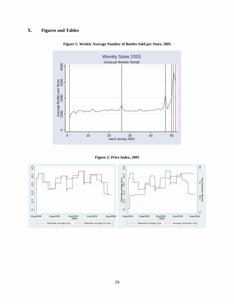
29

X. Figures and Tables

Figure 1: Weekly Average Number of Bottles Sold per Store, 2005

Figure 2: Price Index, 2005

020

0040

0060

0080

00A

vera

ge B

ottle

s pe

r Sto

re

0 10 20 30 40 50week during 2005

Unusual Weeks NotedWeekly Sales 2005

1212

.112

.212

.312

.412

.5

01jan2005 01apr2005 01jul2005 01oct2005 01jan2006ddate

Statewide average price Statewide average list price

7.1

7.15

7.2

7.25

Ave

rage

who

lesa

le c

ost

1212

.112

.212

.312

.412

.5S

tate

wid

e av

erag

e pr

ice

01jan2005 01apr2005 01jul2005 01oct2005 01jan2006ddate

Statewide average price Average wholesale cost

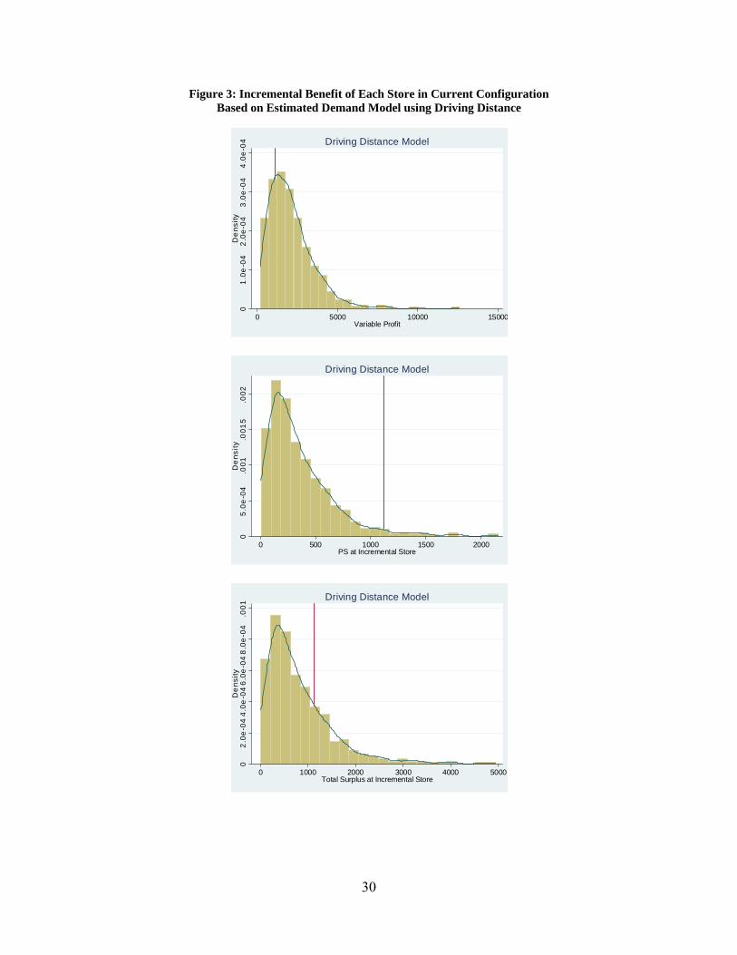
30

Figure 3: Incremental Benefit of Each Store in Current Configuration Based on Estimated Demand Model using Driving Distance

01

.0e

-04

2.0

e-0

43

.0e

-04

4.0

e-0

4D

ens

ity

0 5000 10000 15000Variable Profit

Driving Distance Model

05

.0e

-04

.001

.001

5.0

02D

ens

ity

0 500 1000 1500 2000PS at Incremental Store

Driving Distance Model

02

.0e

-04

4.0

e-0

46

.0e

-04

8.0

e-0

4.0

01D

ens

ity

0 1000 2000 3000 4000 5000Total Surplus at Incremental Store

Driving Distance Model

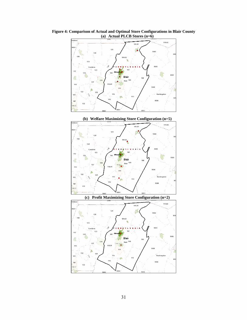
31

Figure 4: Comparison of Actual and Optimal Store Configurations in Blair County (a) Actual PLCB Stores (n=6)

(b) Welfare Maximizing Store Configuration (n=5)

(c) Profit Maximizing Store Configuration (n=2)

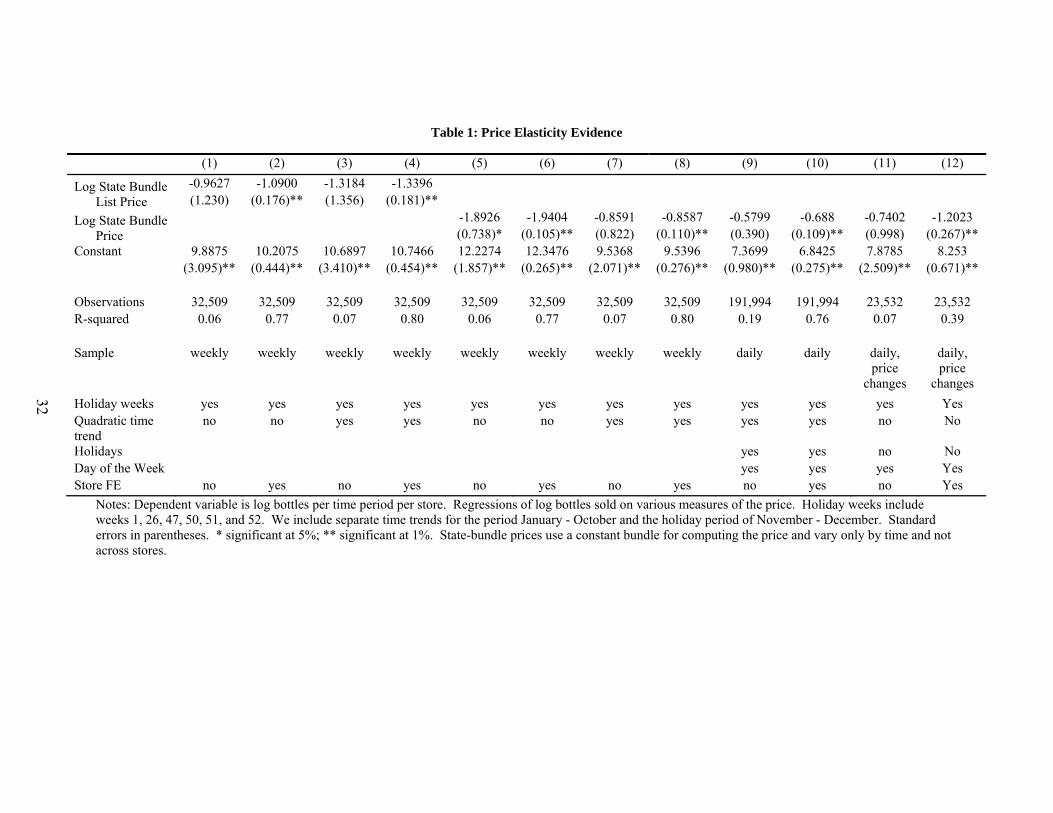
32

Table 1: Price Elasticity Evidence

(1) (2) (3) (4) (5) (6) (7) (8) (9) (10) (11) (12)

Log State Bundle List Price

-0.9627 -1.0900 -1.3184 -1.3396 (1.230) (0.176)** (1.356) (0.181)**

Log State Bundle Price

-1.8926 -1.9404 -0.8591 -0.8587 -0.5799 -0.688 -0.7402 -1.2023 (0.738)* (0.105)** (0.822) (0.110)** (0.390) (0.109)** (0.998) (0.267)**

Constant 9.8875 10.2075 10.6897 10.7466 12.2274 12.3476 9.5368 9.5396 7.3699 6.8425 7.8785 8.253 (3.095)** (0.444)** (3.410)** (0.454)** (1.857)** (0.265)** (2.071)** (0.276)** (0.980)** (0.275)** (2.509)** (0.671)** Observations 32,509 32,509 32,509 32,509 32,509 32,509 32,509 32,509 191,994 191,994 23,532 23,532 R-squared 0.06 0.77 0.07 0.80 0.06 0.77 0.07 0.80 0.19 0.76 0.07 0.39 Sample weekly weekly weekly weekly weekly weekly weekly weekly daily daily daily,

price changes

daily, price

changes Holiday weeks yes yes yes yes yes yes yes yes yes yes yes Yes Quadratic time trend

no no yes yes no no yes yes yes yes no No

Holidays yes yes no No Day of the Week yes yes yes Yes Store FE no yes no yes no yes no yes no yes no Yes

Notes: Dependent variable is log bottles per time period per store. Regressions of log bottles sold on various measures of the price. Holiday weeks include weeks 1, 26, 47, 50, 51, and 52. We include separate time trends for the period January - October and the holiday period of November - December. Standard errors in parentheses. * significant at 5%; ** significant at 1%. State-bundle prices use a constant bundle for computing the price and vary only by time and not across stores.

33

Table 2: Demand, Population, and Distance to the Nearest Store

(1) (2) (3) (4) (5) (6) Average

Daily Sales per Store

Average Log Daily Sales per

Store

Log Daily Sales per

Store

Log Daily Sales per

Store

Log Daily Sales per

Store

Log Daily Sales per

Store

Catchment Area Pop 173.7613 0.4485 0.1873 0.0359 0.1872 0.0359 (12.4713)** (0.0302)** (0.0194)** (0.0007)** (0.0194)** (0.0007)** Average Distance to

Nearest Store -23.8609 -0.0812 -0.0768 -0.0163 -0.0768 -0.0163

(2.8530)** (0.0069)** (0.0066)** (0.0004)** (0.0066)** (0.0004)** Log State Bundle

List Price -0.8458 -0.6573 (0.1759)** (0.1284)**

Log State Bundle Price

-0.6230 -0.6963 (0.1386)** (0.1092)**

Constant 273.7057 5.3648 7.5861 6.7124 7.0251 6.8094 (25.1748)** (0.0609)** (0.4515)** (0.3228)** (0.3930)** (0.2744)** Observations 635 635 191,921 191,921 191,921 191,921 R-squared 0.27 0.33 0.33 0.77 0.33 0.77 Store FE No No No Yes No Yes

Standard errors in parentheses. * significant at 5%; ** significant at 1%.

34

Table 3: Demand Model Estimates

(1) (2) (3)

State-bundle list price -0.1657 -0.1533 -0.1365 (0.0734)** (0.0843)** (0.0932)*

Driving distance -0.0656 (0.0117)***

Straight-line distance -0.1047 (0.0151)***

Driving time -0.0633 (0.0174)***

Black 0.0557 -0.0964 0.0831 (0.0202)*** (0.1434) (0.1990)

Median Income 0.0373 0.0390 0.0330 (0.0051)*** (0.0037)*** (0.0046)***

Median Age 0.0024 0.0047 0.0132 (0.0108) (0.0111) (0.0113)

No Churches per capita -0.1329 -0.2312 (0.0929)* (0.0751)***

Monday 0.7088 0.5966 0.6606 (0.0639)*** (0.0517)*** (0.0834)***

Tuesday 0.7251 0.6542 0.6566 (0.0673)*** (0.0609)*** (0.0845)***

Wednesday 0.8581 0.7595 0.8007 (0.0635)*** (0.0518)*** (0.0828)***

Thursday 1.0132 0.9103 0.9714 (0.0593)*** (0.0517)*** (0.0854)***

Friday 1.5682 1.4668 1.5072 (0.0541)*** (0.0549)*** (0.0832)***

Saturday 1.5857 1.4920 1.5378 (0.0575)*** (0.0468)*** (0.0815)***

Implied elasticity of demand -1.2795 -1.1830 -1.2850 Implied travel cost ($) per

unit 0.3957 0.6827 0.4641 Note: Results based on daily store-level data for a 10% subset (19,255 obs) of all store-day observations. Bootstrapped standard errors (50 replications). We also include separate holiday effects for May 28, June 30-July 3, Sept 3, and Nov. 23-26. Specification (1) uses the shortest travel distance in km along the road network as the measure of distance; specification (2) the straight-line distance in km; and specification (3) the travel time in minutes associated with the shortest travel distance.

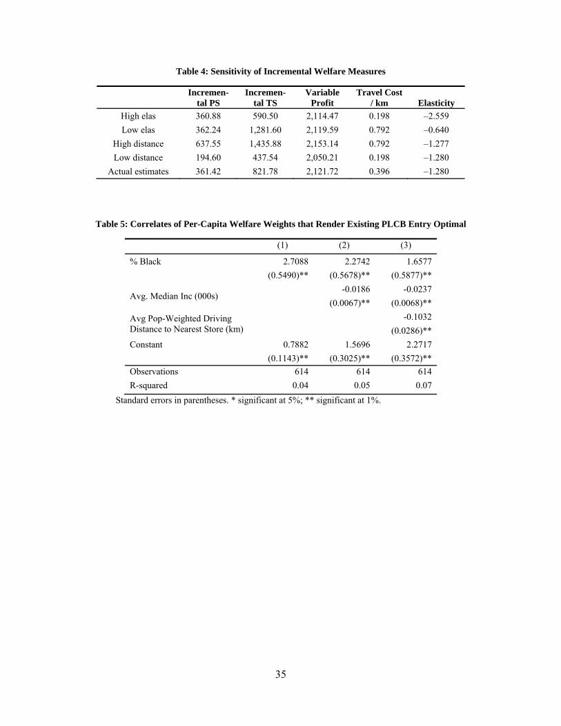
35

Table 4: Sensitivity of Incremental Welfare Measures

Incremen-tal PS

Incremen-tal TS

Variable Profit

Travel Cost / km Elasticity

High elas 360.88 590.50 2,114.47 0.198 –2.559 Low elas 362.24 1,281.60 2,119.59 0.792 –0.640

High distance 637.55 1,435.88 2,153.14 0.792 –1.277 Low distance 194.60 437.54 2,050.21 0.198 –1.280

Actual estimates 361.42 821.78 2,121.72 0.396 –1.280

Table 5: Correlates of Per-Capita Welfare Weights that Render Existing PLCB Entry Optimal

(1) (2) (3)

% Black 2.7088 2.2742 1.6577 (0.5490)** (0.5678)** (0.5877)**

Avg. Median Inc (000s) -0.0186 -0.0237

(0.0067)** (0.0068)**

Avg Pop-Weighted Driving Distance to Nearest Store (km)

-0.1032 (0.0286)**

Constant 0.7882 1.5696 2.2717 (0.1143)** (0.3025)** (0.3572)**

Observations 614 614 614 R-squared 0.04 0.05 0.07

Standard errors in parentheses. * significant at 5%; ** significant at 1%.

36

Table 6: Comparison of Regimes

County Regime # of

Stores Total Profit

Net Welfare

Quantity Sold

Welf rel to Max

% Δ Welf†

Berks Actual 14 20,897 334,221 7,208 -1.31% -4.99% (pop: 373,638) Profit Maximization 5 26,323 331,862 6,294 -2.01% -7.63%

Welf. Maximization 18 21,185 338,673 8,147

Blair Actual 6 3,063 109,078 1,927 -3.07% -14.48% (pop: 129,144) Profit Maximization 2 6,742 111,765 1,771 -0.68% -3.22%

Welf. Maximization 5 5,218 112,532 2,132

Lancaster Actual 15 22,735 396,944 7,791 -2.21% -9.32% (pop: 470,658) Profit Maximization 7 30,284 402,744 7,517 -0.79% -3.31%

Welf. Maximization 14 27,328 405,933 8,477

Lycoming Actual 7 1,768 99,803 1,892 -2.58% -11.29% (pop: 120,044) Profit Maximization 2 5,871 102,025 1,599 -0.41% -1.80%

Welf. Maximization 4 4,813 102,446 1,831

Schuylkill Actual 10 -391 133,291 2,128 -5.56% -29.79% (pop: 157,342) Profit Maximization 3 7,080 140,195 2,058 -0.67% -3.58%

Welf. Maximization 10 3,105 141,137 2,817 †The change in welfare is expressed as a percentage of the consumers’ expenditure under the welfare maximizing configuration.

Table 7: Distribution of Distance Traveled to Closest Store, Alternative Configurations

County Actual Welfare-

Max Profit-Max

Targeted Welf-Max

Regulated Private Entry

Berks 5.825 3.305 8.099 4.236 5.936 Blair 6.764 4.312 8.732 3.840 5.818

Lancaster 6.077 4.656 7.022 4.529 5.795 Lycoming 6.083 7.305 10.187 4.508 7.243 Schuylkill 5.527 4.541 10.530 4.541 5.160

Total 6.010 4.455 8.358 4.357 5.892

37

Table 8: Performance of Myopic Algorithm

county obj func No

stores net welf Q profit net welf

dev† profit dev†

Berks profit max 5 331,862 6,294 26,323 0.00% Blair profit max 2 111,409 1,740 6,584 -2.34%

Lancaster profit max 7 402,594 7,506 30,230 -0.18% Lycoming profit max 2 102,025 1,599 5,871 0.00% Schuylkill profit max 3 140,195 2,058 7,080 0.00%

Berks welfare max 17 338,125 8,006 21,587 -0.16% Blair welfare max 5 112,341 2,115 5,133 -0.17%

Lancaster welfare max 14 405,890 8,473 27,309 -0.01% Lycoming welfare max 4 102,353 1,824 4,775 -0.09% Schuylkill welfare max 7 141,767 2,579 5,251 0.45%

†The welfare (profit) deviations are calculated as the percentage change in welfare (profit) in going from the welfare (profit) under the welfare (profit) maximizing configuration to the welfare (profit) under the configuration predicted by the myopic algorithm to maximize welfare (profit).

Table 9: Whole State Summary

System's Size Method N Profit Net

Welfare Quantity Average Distance

Profit Maximization SME(profit) 185 971,076 11,329,609 232,321 7.46 Welfare

Maximization SME(welfare) 394 887,189 11,437,280 261,853 4.63

Actual size† 616 614,607 11,130,868 257,033 4.84 †We exclude 8 stores without or with incorrect location information.

38

Table 10: Regime Comparison: Constrained Welfare Maximization, Regulated Private Entry, and Free Entry*

County Regime # of

StoresTotal Profit

Net Welfare

Quantity Sold

Welf rel to max

Δ Welf as % of Welf Max Exp†

Berks Constr. Welf. Maximization 14 23,466 338,153 7,715 (pop: 373,638) Regulated Entry 14 21,359 335,007 7,299 -0.93% -3.29%

Free Entry 29 10,403 323,487 8,445 -4.34% -15.35%

Blair Constr. Welf. Maximization 6 4,468 112,253 2,204 (pop: 129,144) Regulated Entry 6 3,572 110,232 2,027 -1.80% -7.41%

Free Entry 8 2,231 108,270 2,204 -3.55% -14.60%

Lancaster Constr. Welf. Maximization 15 26,657 405,837 8,565 (pop: 470,658) Regulated Entry 15 24,461 400,873 8,132 -1.22% -4.68%

Free Entry 31 11,691 387,853 9,141 -4.43% -12.28%

Lycoming Constr. Welf. Maximization 7 2,772 102,056 2,090 (pop: 120,044) Regulated Entry 7 1,816 99,912 1,901 -2.10% -8.29%

Free Entry 6 2,624 99,014 1,840 -2.98% -11.76%

Schuylkill Constr. Welf. Maximization 10 3,105 141,137 2,817 (pop: 157,342) Regulated Entry 10 2,588 139,928 2,715 -0.86% -3.47%

Free Entry 8 3,135 136,577 2,382 -3.23% -9.61% †The change in welfare from free or regulated entry is expressed as a percentage of the consumers’ expenditure under the welfare maximizing configuration. *Both regulated free entry and constrained welfare maximization refer to scenarios where the number of stores is fixed to be equal to the number of stores actually operating in each of the county markets.

39

XI. References

Berry, Steven T., “Estimation of a Model of Entry in the Airline Industry.” Econometrica 60 (1992): 889-917.

Berry, Steven T. and Joel Waldfogel, “Free Entry and Social Inefficiency in Radio Broadcasting.” RAND Journal of Economics 30(3) (1999): 397-420.

Berry, Steven T. and Joel Waldfogel, “Mergers and Product Variety.” Quarterly Journal of Economics 116 (2001): 1009-1025.

Boardman, Anthony E., and Vining, Aidan R. “Ownership and performance in competitive environments: A comparison of the performance of private, mixed, and state-owned enterprises.” Journal of Law and Economics 32 (1989): 1-33.

Bös, Dieter. “Public Sector Pricing.” In Handbook of Public Economics, A.J. Auerbach and M. Feldstein, eds. North Holland, Amsterdam. 1985.

Bresnahan, Timothy F. and Peter C. Reiss, “Entry and Competition in Concentrated Markets.” Journal of Political Economy 99 (1991): 977-1009.

Chaloupka, Frank J., Michael Grossman, and Henry Saffer, “The Effects of Price on Alcohol Consumption and Alcohol-Related Problems.” Alcohol Research and Health 6(1) (2002): 22-34.

Chan, Tat Y., V. Padmanabhan, and P.B. Seetharaman, “An Econometric Model of Location and Pricing in the Gasoline Market.” Journal of Marketing Research XLIV (2007): 622-635.

Cook, Phillip J. and Michael J. Moore, “Alcohol.” NBER Working Paper 6905 (1999).

Daskin, Mark, Network and Discrete Location: Models, Algorithms and Applications, John Wiley and Sons, Inc., New York. 1995.

Davis, Peter, “Spatial competition in retail markets: movie theaters.” RAND Journal of Economics 37(4) (2006): 964-982.

de Palma, André, Victor Ginsburgh, and J-F. Thisse, “On the Existence of Location Equilibria in the 3-Firm Hotelling Problem.” Journal of Industrial Economics 36 (1987): 245-252.

Dixit, Avinash and Joseph E. Stiglitz, “Monopolistic Competition and Optimum Product Diversity.” American Economic Review 67 (1977): 297-308.

40

Fudenberg, Drew and David K. Levine. The Theory of Learning in Games, MIT Press, Cambridge, MA. 1998.

Hotelling, Harold, “Stability in Competition,” The Economic Journal 39(153) (1929): 41-57.

Houde, Jean-Francois, “Spatial differentiation in retail markets for gasoline,” mimeo. University of Wisconsin-Madison (2009).

Mankiw, N. Gregory and Michael D. Whinston, “Free Entry and Social Inefficiency.” RAND Journal of Economics 17(1) (1986): 48-58.

Mazzeo, Michael, “Product Choice and Oligopoly Market Structure.” RAND Journal of Economics 33(2) (2002): 241-242.

McManus, Brian, “Nonlinear Pricing in an Oligopoly Market: the Case of Specialty Coffee.” RAND Journal of Economics 38(3) (2007): 512-532.

Perl, Jossef and Peng-Kuan Ho, “Public Facilities Location under Elastic Demand.” Transportation Science 24(2) (1990): 117-136.

Samuelson, Larry. Evolutionary Games and Equilibrium Selection. MIT Press, Cambridge. 1997.

Seim, Katja, “An Empirical Model of Firm Entry with Endogenous Product-type Choices.” RAND Journal of Economics 37(3) (2006): 619-640.

Small, Kenneth and Harvey Rosen, “Applied Welfare Economics with Discrete Choice Models.” Econometrica 49(1) (1981): 105-130.

Spence, Michael, “Product Selection, Fixed Costs, and Monopolistic Competition.” Review of Economic Studies 43 (1976): 217-236.

Steiner, Peter, “Program Patterns and the Workability of Competition in Radio Broadcasting,” Quarterly Journal of Economics 66 (1952): 194-223.

Sweeting, Andrew, “The Effects of Mergers on Product Positioning: Evidence from the Music Radio Industry.” RAND Journal of Economics, forthcoming (2009).

Thomadsen, Raphael, “The Effect of Ownership Structure on Prices in Geographically Differentiated Industries,” RAND Journal of Economics, 36(4) (2005): 908-929.