JHEP07(2017)058

Published for SISSA by Springer

Received: June 9, 2017

Accepted: July 4, 2017

Published: July 12, 2017

(Higgs) vacuum decay during inflation

Aris Joti,a Aris Katsis,a Dimitris Loupas,a Alberto Salvio,b Alessandro Strumia,b,c

Nikolaos Tetradisa and Alfredo Urbanob

aDepartment of Physics, National and Kapodistrian University of Athens,

Zographou 157 84, GreecebCERN, Theoretical Physics Department,

Geneva, SwitzerlandcDipartimento di Fisica, Universita di Pisa and INFN, Sezione di Pisa,

Largo Bruno Pontecorvo 3, Pisa, Italy

E-mail: apjoti@gmail.com, Aris Katsis@hotmail.com,

dloupas@physics.auth.gr, alberto.salvio@cern.ch, astrumia@cern.ch,

ntetrad@phys.uoa.gr, alfredo.leonardo.urbano@cern.ch

Abstract: We develop the formalism for computing gravitational corrections to vacuum

decay from de Sitter space as a sub-Planckian perturbative expansion. Non-minimal cou-

pling to gravity can be encoded in an effective potential. The Coleman bounce continuously

deforms into the Hawking-Moss bounce, until they coincide for a critical value of the Hub-

ble constant. As an application, we reconsider the decay of the electroweak Higgs vacuum

during inflation. Our vacuum decay computation reproduces and improves bounds on the

maximal inflationary Hubble scale previously computed through statistical techniques.

Keywords: Higgs Physics, Solitons Monopoles and Instantons, Renormalization Group,

Classical Theories of Gravity

ArXiv ePrint: 1706.00792

Open Access, c© The Authors.

Article funded by SCOAP3.https://doi.org/10.1007/JHEP07(2017)058

JHEP07(2017)058

Contents

1 Introduction 1

2 General theory and sub-Planckian approximation 2

2.1 The Hawking-Moss bounce 5

2.2 Sub-Planckian approximation to the bounce 5

3 Renormalizable potential 8

3.1 Zeroth order in H,M MPl 8

3.2 First order in H,M MPl 10

3.3 Effect of non-minimal couplings 11

4 Standard Model vacuum decay during inflation 12

4.1 SM vacuum decay for small H 13

4.2 SM vacuum decay for large H hcr 13

4.3 SM vacuum decay for H ∼ hcr 15

5 Conclusions 17

1 Introduction

A false vacuum can decay through quantum tunnelling that leads to nucleation of regions

of true vacuum. The rate of this non-perturbative phenomenon is exponentially suppressed

by the action of the ‘bounce’, the field configuration that dominates the transition [1].

Coleman and de Luccia showed how to account for gravitational effects [2]. Their

formalism can be simplified by restricting to sub-Planckian energies, which are the only

ones for which Einstein gravity can be trusted. Simplified expressions were obtained in [3, 4]

for the decay of flat space-time.

We extend here the simplified formalism to tunnelling from de Sitter space (positive

energy density), which is relevant during inflation with Hubble constant H. It is known

that gravitational effects can dramatically enhance the tunnelling rate. The qualitative

intuition is that a de Sitter space has a Gibbons-Hawking ‘temperature’ T = H/2π [5] that

gives extra ‘thermal’ fluctuations that facilitate tunnelling. Equivalently, light scalar fields

h undergo fluctuations δh ∼ H/2π per e-folding.

We show that tunnelling from de Sitter can be described by a simplified formalism

assuming that H and the bounce energy density are sub-Planckian. We also show how to

include perturbatively the small extra Planck-suppressed corrections due to gravity.

Vacuum decay in the presence of gravity receives an extra contribution from another

bounce, known as the Hawking-Moss (HM) solution: a constant field configuration that

sits at the top of the potential barrier [6]. Being constant, it has the higher O(5) symmetry

of 4-dimensional de Sitter space, while the Coleman-de Luccia (CdL) bounce is only O(4)

– 1 –

JHEP07(2017)058

symmetric. The Hawking-Moss contribution to vacuum decay vanishes for flat space, which

corresponds to H = 0. We show that the Coleman bounce continuously deforms into the

Hawking-Moss bounce, and the two become equal at a critical value of H, usually equal to

1/2 of the curvature of the potential at its maximum.

Furthermore, the simplified formalism allows to easily include perturbatively the effect

of a general non-minimal scalar coupling to gravity, as a modification of the effective scalar

potential.

The above features are relevant for the possible destabilization of the Standard Model

(SM) vacuum during inflation. The Higgs field can fluctuate towards values a few orders

of magnitude below the Planck scale, for which its potential can be deeper than for the

electroweak vacuum [7–23]. If vacuum decay happens during inflation, the regions of true

vacuum expand and engulf the whole space [2, 18, 24]. This catastrophic scenario is avoided

if H is small enough that vacuum decay is negligibly slow. The derivation of a precise bound

on the scale of inflation has been based mainly on a stochastic approach, relying on the

numerical solution of Fokker-Planck or Langevin equations that describe the real-time evo-

lution of fluctuations in the scalar field. We pursue here the alternative approach of comput-

ing the Euclidean tunnelling rate. We reproduce some previous results and correct others.

The paper is structured as follows. In section 2 we derive a simple approximation for

sub-Planckian vacuum decay. In section 3 we validate the analytical expressions by focusing

on a toy renormalizable scalar potential, and show how the Coleman bounce connects to

the Hawking-Moss bounce. In the final section 4 we obtain bounds on the scale of inflation

H by computing the tunnelling rate, dominated by the Hawking-Moss bounce. Conclusions

are given in section 5.

2 General theory and sub-Planckian approximation

Coleman and de Luccia [2] developed the formalism for computing vacuum decay from a

de Sitter space with Hubble constant H taking gravity into account. In this section we

review this formalism, extend it to a general non-minimal coupling of the Higgs to gravity

and then derive simplified expressions that hold in the sub-Planckian limit H,M MPl,

where M is the mass scale that characterises the scalar potential and thereby the bounce.

Within Einstein gravity this approximation applies to all cases of interest: indeed, Einstein

gravity is non-renormalizable and must be replaced by some more fundamental theory at

the Planck scale or below it. Furthermore, the Hubble constant during inflation must be

sub-Planckian to reproduce the smallness of the inflationary tensor-to-scalar ratio.

Coleman and de Luccia assumed that the space-time probability density of vacuum

decay is exponentially suppressed by the action of a ‘bounce’ configuration, like in flat

space.1 We consider the Euclidean action of a scalar field h(x) in the presence of gravity,

S =

∫d4x√

det g

[1

2(∇h)2 + V (h)− R

16πG− f(h)

2R], (2.1)

1The proof valid in flat space cannot be extended to de Sitter space because the Hamiltonian is not

well defined. One cannot isolate the ground state by computing a transition amplitude in the limit of

infinite time, because Euclidean de Sitter has finite volume, so that multi-bounce configurations cannot be

resummed in a dilute gas approximation.

– 2 –

JHEP07(2017)058

where G ≡ 1/M2Pl ≡ 1/(8πM2

Pl) ≡ κ/8π is the Newton constant, with MPl ≈ 2.43 ×1018 GeV. For the time being V and f are generic functions of the scalar field h. The

action in eq. (2.1) is the most general action for the metric gµν and h up to two-derivative

terms: an extra generic function Z(h) multiplying the kinetic term of the scalar field can

be removed by redefining h. The classical equations of motion for gravity and for h are [25]

(M2Pl + f)

(Rµν −

gµν2R)

= ∇µh∇νh− gµν[

(∇h)2

2+ V +∇2f

]+∇µ∇νf , (2.2)

∇2h+1

2

df(h)

dhR =

dV (h)

dh, (2.3)

where ∇2 = ∇µ∇µ. The use of these equations allows us to simplify the action. Taking

the trace of eq. (2.2) one finds(M2

Pl + f(h))R = (∇h)2 + 4V (h) + 3∇2f(h). (2.4)

Substitution in eq. (2.1) gives

S = −∫d4x√

det g

[V (h) +

3

2∇2f(h)

]. (2.5)

The second term in the above expression is reduced to a boundary term upon integration.

For the problem at hand this term vanishes and one obtains

S = −∫d4x√

det g V (h). (2.6)

We are interested in the possible decay of the false vacuum during a period in which the

vacuum energy is dominated by a cosmological constant V0. We assume that V (h) has two

minima, a false vacuum at h = hfalse and the true vacuum at h = htrue, with htrue > hfalse.

In the following we will set hfalse = 0 without loss of generality. The two minima are

separated by a maximum of the potential. We identify V0 = V (0) and split the potential as

V (h) = V0 + δV (h), (2.7)

such that δV (0) = 0. The vacuum energy density V0 induces a de Sitter space with curva-

ture R = 12H2, where the Hubble rate H is given by

H2 =V0

3M2Pl

(2.8)

(we assume without loss of generality f(0) = 0: a non-vanishing value of f(0) can be ab-

sorbed in a redefinition of κ). In the following we will collectively denote with Φfalse the field

configuration with this de Sitter background and h = 0. In the semiclassical (small ~) limit

the decay rate Γ of the false vacuum per unit of space-time volume V is given by [1, 2, 26, 27]

dΓ

dV= Ae−S/~(1 +O(~)), (2.9)

– 3 –

JHEP07(2017)058

where A is a quantity of order M4, where M is the mass scale in the potential. The

dominant effect is the bounce action S. It is given by

S = S(ΦB)− S(Φfalse), (2.10)

where ΦB is an unstable ‘bounce’ solution of the Euclidean equations of motion, such that

S is finite and there is no other configuration with the same properties and lower S. In the

rest of the paper we set the units such that ~ = 1. In order to find ΦB we follow [2] and

introduce an O(4)-symmetric Euclidean ansatz for the Higgs field h(r) and for the geometry

ds2 = dr2 + ρ(r)2dΩ2, (2.11)

where dΩ is the volume element of the unit 3-sphere. On this background, the action

becomes

S = 2π2∫drρ3

[(h′2

2+ V (h)

)− R

2κ− R

2f(h)

], (2.12)

where the curvature is

R = − 6

ρ3(ρ2ρ′′ + ρρ′2 − ρ) (2.13)

and a prime denotes d/dr. The simplified action of eq. (2.6) becomes:

S = −2π2∫dr ρ3 V (h). (2.14)

The equations of motion are

h′′ + 3ρ′

ρh′ =

dV (h)

dh− 1

2

df(h)

dhR, (2.15)

ρ′2 = 1 +κρ2

3(1 + κf(h))

(1

2h′2 − V (h)− 3

ρ′

ρ

df(h)

dhh′). (2.16)

Let us discuss the boundary conditions. Since in the false vacuum the space is a 4-sphere

and topology cannot be changed dynamically, the space described by ρ will have the same

topology; thus ρ will have two zeros. One can be conventionally chosen to occur at r = 0,

and the other one at some value of r that we call rmax,

ρ(0) = ρ(rmax) = 0. (2.17)

The whole space is covered by the coordinate interval [0, rmax]. In the de Sitter case one

has rmax = π/H. The equation of motion of h in (2.15) and the regularity of h at r = 0

and r = rmax imply

h′(0) = h′(rmax) = 0. (2.18)

In the limit of small H (i.e. large rmax), the boundary condition h′(rmax) = 0 implies

h(∞) = 0 in view of the large volume outside the core of the bounce. Generically, in a non-

trivial (r-dependent) bounce h(r) does not tend to the false vacuum solution, hfalse = 0,

as r → rmax, unless we are in the flat space case, rmax →∞.2

2This can be shown whenever h and ρ are regular functions at r = rmax: by Taylor-expanding

the equations of motion eqs. (2.15)–(2.16) around r = rmax, using h(r) =∑∞

n=1 cn(r − rrmax)n and

ρ(r) =∑∞

n=1 an(r − rmax)n: one obtains a set of algebraic equations that force cn = 0. Namely, for

rmax < ∞, the only regular function that goes indefinitely close to the false vacuum solution as r → rmax

is the false vacuum solution itself.

– 4 –

JHEP07(2017)058

2.1 The Hawking-Moss bounce

The Hawking-Moss configuration [6], which we denote with ΦHM, is a simple unstable

finite-action solution satisfying the equations of motion and boundary conditions above.

In this configuration the scalar sits at the constant value h = hmax that maximizes3

VH(h) ≡ V (h)− 6H(hmax)2f(h), (2.19)

where H(h) is the Hubble constant given by

H2(h) =κV (h)

3(1 + κf(h)). (2.20)

The Hawking-Moss solution exists whenever VH has a maximum. When f = 0, hmax

coincides with the maximum of the potential. We can compute the tunnelling rate by

using the simplified action in eq. (2.14), obtaining for the Hawking-Moss solution

SHM = S(ΦHM)− S(Φfalse) = 24π2M4Pl

[1

V0− (1 + κf(hmax))2

V (hmax)

]. (2.21)

Defining VH(h) = V0 + δVH(h), in the limit δV (hmax) V0 and at leading order in κ this

formula simplifies to

SHM '8π2

3

δVH(hmax)

H4, (2.22)

where H can be evaluated at h = 0. We shall examine the role of the Hawking-Moss

solution for vacuum decay, finding that it is relevant for large values of H.

Generically, there are also non-trivial solutions with a non-constant Higgs profile h(r),

which, in the flat-space limit, reduce to the Coleman bounce [1]. In order to determine

the various bounces, one must solve the coupled eqs. (2.15) and (2.16) with the boundary

conditions described above.

2.2 Sub-Planckian approximation to the bounce

The problem can be simplified by using the low-energy approximation, which, as explained

at the beginning of this section, is not physically restrictive if one works within the regime

of validity of Einstein gravity (as we do). We illustrate now such an approximation.

The low-energy approximation consists in assuming that gravity is weak in the sense

that

H,1

RMPl , (2.23)

where R is the size of the bounce (1/R is roughly given by the mass scale that appears

in the scalar potential V ). The two conditions arise because gravitational corrections are

3The Coleman bounce is O(4)-symmetric. The Hawking-Moss bounce, having a constant h, has the full

O(5) symmetry of de Sitter space. Vacuum decay at finite-temperature T is described by a configuration

with period 1/T in the Euclidean time coordinate. At large T , the thermal bounce becomes constant in

time, acquiring a O(3) ⊗ O(2) symmetry (see [4] for a recent discussion). These are different solutions: a

de Sitter space with Hubble constant H is qualitatively similar but not fully equivalent to a thermal bath

at temperature T = H/2π.

– 5 –

JHEP07(2017)058

suppressed by powers of the Planck mass, and are thereby small if the massive parameters

of the problem are small in Planck units. During inflation, the condition on H is satisfied

in view of the experimental constraint H < 3.6 × 10−5MPl (see section 5.1 of [28]). The

first condition is also not restrictive because it is necessary to avoid energies of order of the

Planck scale, for which Einstein’s theory breaks down.

Assuming that these conditions are satisfied, we expand h and ρ in powers of κ=1/M2Pl:

h(r) = h0(r) + κh1(r) +O(κ2), ρ(r) = ρ0(r) + κρ1(r) +O(κ2). (2.24)

The leading-order metric corresponds to de Sitter space:

ρ0(r) =sin(Hr)

H. (2.25)

Furthermore, we are interested in a situation in which H ∼ 1/R: otherwise one can neglect

H and return to the flat space approximation discussed in [4, 18]. Thus we are in a regime

in which the vacuum energy is dominated by V0 = 3H2M2Pl δV (h) and the gravitational

background is perturbed only slightly by the bounce h(r).

The equation of motion of the zeroth order bounce h0(r) (that is the equation on the

de Sitter non-dynamical background) and the first correction ρ1 to the metric function can

be obtained by inserting the expansion of eq. (2.24) in eqs. (2.15) and (2.16). The de Sitter

bounce h0(r) at zeroth order in κ is given by

h′′0 + 3H cot(Hr)h′0 =dVH(h0)

dh, (2.26)

where VH is given in eq. (2.19), where H can be evaluated at h = 0 rather than at

hmax: since the difference is an higher order effect in κ, we avoid introducing two different

symbols.4 The boundary conditions are

h′(0) = h′(π/H) = 0. (2.28)

At this lowest order, the effect of a general non-minimal coupling to gravity f(h) is equiva-

lent to replacing the potential V (h) with the modified potential VH(h) given in eq. (2.19).

The equation for ρ1 is(ρ1

cos(Hr)

)′=

tan2Hr

6H2

(h′202− δV (h0) + 3H2f(h0)−

3H

tanHr

df(h0)

dhh′0

)(2.29)

such that ρ1(r) can be obtained by solving either by integration starting from ρ1(0) = 0 (al-

though some care is needed to handle apparent singularities at rH = π/2), or by converting

4As an aside comment, an O(4)-symmetric space is conformally flat, such that by performing a Weyl

transformation one can revert to flat-space equations with a Weyl-transformed action. A de Sitter space is

conformally flat when written in terms of conformal time r ≡ 2 tan(Hr/2)/H. Performing the associated

Weyl transformation h0(r) = h0(r)/ cos2(Hr/2), the bounce equation (2.26) becomes

d2h0

dr2+

3

r

dh0

dr=V (1)(h0(1 +H2r2/4))

(1 +H2r2/4)3, V ≡ VH −H2h2 = V −H2(6f + h2) (2.27)

where V (n) is the n-th derivative of V .

– 6 –

JHEP07(2017)058

eq. (2.29) into a 1st-order linear differential equation that can be solved numerically. In

the limit where the bounce has a size R much smaller than 1/H, the solution

ρ1(r)R1/H' cos(Hr)

∫ r

0drr2

6

(1

2h′20 − δV (h0)−

3

r

df(h0)

dhh′0

)(2.30)

reduces to the flat-space solution of [4], times the overall cos(Hr) factor.

Our goal now is to compute the action (difference) S of eq. (2.10) because, which is

the quantity that appears in the decay rate. The expansion for the fields in (2.24) leads to

a corresponding expansion of S in powers of κ:

S = S0 + κS1 +O(κ2). (2.31)

The zeroth order action is5

S0 = 2π2∫ π/H

0dr

sin3Hr

H3

[h′202

+ δVH(h0)

]. (2.32)

The leading correction due to gravity, ∆Sgravity ≡ κS1, is

∆Sgravity =6π2

M2Pl

∫ π/H

0dr

[sin2(Hr)

H2ρ1

(h′202

+ δV (h0)− 3H2f(h0)

)− sin(Hr)

Hρ′21 +

+ 2H sin(Hr)ρ21 +sin2(Hr)

H2f(h0)

(2H cot(Hr)ρ′1 + ρ′′1

)]. (2.33)

The expression of ∆Sgravity above has been simplified by using the equation of h0 in (2.26)

and by an integration by parts. It can be further simplified as follows. Rescaling

ρ1(r)→ sρ1(r) corresponds to shifting ρ1(r) by (s− 1)ρ1(r). By noticing that (s− 1)ρ1(r)

is a particular variation δρ1 we conclude that the action must have an extremum at s = 1.

Applying this argument to eq. (2.33) relates the integrals of terms linear and quadratic in

ρ1. The final simplified expression is:

∆Sgravity =6π2

M2Pl

∫ π/H

0dr

sin(Hr)

H

[ρ′21 − 2H2ρ21

]. (2.34)

Note that the upper integration limit is simply π/H. In deriving it we have taken into

account the dynamics of the spacetime volume: the shift in rmax does not affect the inte-

gral because the integrand contains a function, sinHr, which vanishes at the integration

boundaries.6

5The action contains the curvature term enhanced by negative powers of the Planck mass. The O(1/κ)

term cancels in the difference defining S, eq. (2.10). Moreover, it leads to a term involving ρ1 in the

integrand of S0 proportional to (sin(Hr)2ρ′1)′. However, this total-derivative term gives no contribution to

S0 for a ρ′1 that is regular at r = 0 and π/H.6The correction to ρ generates a corresponding correction in rmax, defined around eq. (2.17). Indeed

0 = ρ(rmax) = ρ0(rmax) + κρ1(rmax) +O(κ2) (2.35)

tells us that rmax is a function of κ that can be expanded around κ = 0: rmax = π/H + κr1 +O(κ2). By

inserting the last expansion in eq. (2.35) we obtain κρ′0(π/H)r1 + κρ1(π/H) + O(κ2) = 0. Noticing that

ρ′0(π/H) = −1, we find r1 = ρ1(π/H), where ρ1(π/H) can be obtained from the solution of eq. (2.29).

– 7 –

JHEP07(2017)058

In the limit H → 0, eq. (2.34) reduces to the flat-space expression found in [4], which

is positive-definite, unlike the result for generic H. Just like on flat space, ∆Sgravity is

independent of h1 on-shell: the reason is that the only way h1 could appear at first-order

in κ is by taking the first variation of the h-dependent part of the action, eq. (2.12), but

this vanishes when h0 solves eq. (2.26).

In conclusion, eqs. (2.26), (2.29), (2.32) and (2.34) tell us that, in order to compute the

semiclassical decay rate including the first-order gravitational corrections, one just needs to

compute the bounce h0 on the background de Sitter space. This is easier than solving the

coupled equations for the bounce and the geometry in eqs. (2.15) and (2.16). Being a one-

dimensional problem, it can be solved through an over-shooting/under-shooting method.

Then, one needs to plug h0 in the expression for ρ1 to get S0 +∆Sgravity. One can therefore

focus on the equation of h0. Imposing the boundary conditions in eq. (2.28) leads to

well-defined solutions, as we will show in the next sections.

3 Renormalizable potential

In order to understand the influence of the de Sitter background on vacuum decay, we

perform a numerical study of the problem for a toy renormalizable potential

V (h) = V0 +M2

2h2 − A

3h3 +

λ

4h4 (3.1)

with M2 = λhmaxhtrue and A = λ(hmax + htrue), such that the potential has a maximum

at h = hmax and two vacua at h = 0 and at h = htrue: the latter vacuum is the true

deeper vacuum provided that htrue > 2hmax > 0. Quantum corrections are perturbatively

small when λ 4π and A 4πM . The curvature of the potential at its maximum is

µ2 ≡ −V (2)(hmax) = λ(htrue − hmax)hmax. The constant term V0 gives a Hubble constant

H through eq. (2.8).

3.1 Zeroth order in H,M MPl

The main qualitative influence of the Hubble rate H on vacuum decay is most easily

understood at zeroth order in the sub-Planckian expansion, ignoring the gravitational

corrections that will be discussed in the next section.

We consider a typical illustrative example: vanishing non-minimal coupling to gravity

(introduced later), λ = 0.6 and htrue = 3hmax. In figure 1 we show the resulting bounces

h0(t) at zeroth order in H,M MPl for increasing values of H.

For H M the de Sitter radius 1/H is much larger than the scale of the flat-space

bounce, of order 1/M . Thereby, the flat space bounce is negligibly affected by the curvature

of the space, fitting comfortably into a horizon.

We see that the critical value above which H starts influencing the bounce action is

of order M . Thereby the bounce correction to the energy density is of order M4, which

is negligible with respect to V0 = 3M2PlH

2. This confirms that, in the relevant range,

the bounce correction to the background is negligible, being Planck suppressed, so that it

makes sense to first consider the zeroth-order approximation.

– 8 –

JHEP07(2017)058

()/

/ =

/ =

/ =

/ =

/ =

/ =

/ =

-

/

+κ

/ =

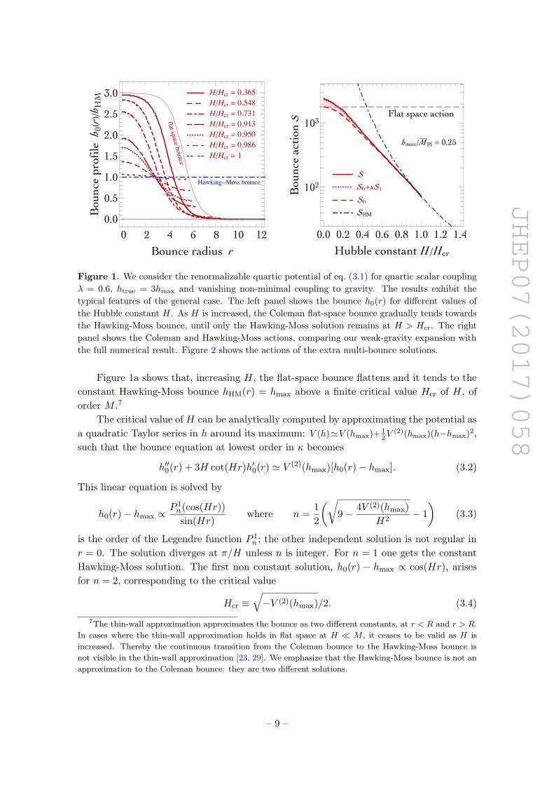
Figure 1. We consider the renormalizable quartic potential of eq. (3.1) for quartic scalar coupling

λ = 0.6, htrue = 3hmax and vanishing non-minimal coupling to gravity. The results exhibit the

typical features of the general case. The left panel shows the bounce h0(r) for different values of

the Hubble constant H. As H is increased, the Coleman flat-space bounce gradually tends towards

the Hawking-Moss bounce, until only the Hawking-Moss solution remains at H > Hcr. The right

panel shows the Coleman and Hawking-Moss actions, comparing our weak-gravity expansion with

the full numerical result. Figure 2 shows the actions of the extra multi-bounce solutions.

Figure 1a shows that, increasing H, the flat-space bounce flattens and it tends to the

constant Hawking-Moss bounce hHM(r) = hmax above a finite critical value Hcr of H, of

order M .7

The critical value of H can be analytically computed by approximating the potential as

a quadratic Taylor series in h around its maximum: V (h)'V (hmax)+ 12V

(2)(hmax)(h−hmax)2,

such that the bounce equation at lowest order in κ becomes

h′′0(r) + 3H cot(Hr)h′0(r) ' V (2)(hmax)[h0(r)− hmax]. (3.2)

This linear equation is solved by

h0(r)− hmax ∝P 1n(cos(Hr))

sin(Hr)where n =

1

2

(√9− 4V (2)(hmax)

H2− 1

)(3.3)

is the order of the Legendre function P 1n ; the other independent solution is not regular in

r = 0. The solution diverges at π/H unless n is integer. For n = 1 one gets the constant

Hawking-Moss solution. The first non constant solution, h0(r) − hmax ∝ cos(Hr), arises

for n = 2, corresponding to the critical value

Hcr ≡√−V (2)(hmax)/2. (3.4)

7The thin-wall approximation approximates the bounce as two different constants, at r < R and r > R.

In cases where the thin-wall approximation holds in flat space at H M , it ceases to be valid as H is

increased. Thereby the continuous transition from the Coleman bounce to the Hawking-Moss bounce is

not visible in the thin-wall approximation [23, 29]. We emphasize that the Hawking-Moss bounce is not an

approximation to the Coleman bounce: they are two different solutions.

– 9 –

JHEP07(2017)058

=

=

=

=

/

/

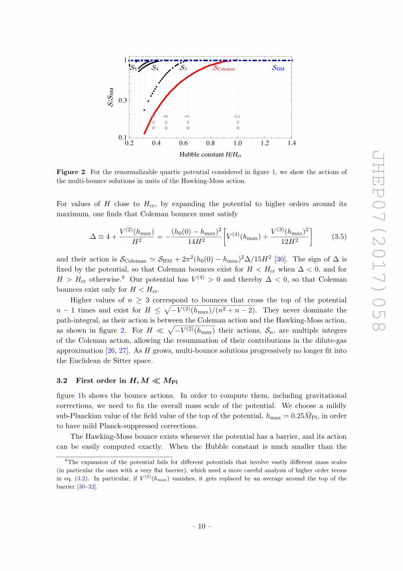
Figure 2. For the renormalizable quartic potential considered in figure 1, we show the actions of

the multi-bounce solutions in units of the Hawking-Moss action.

For values of H close to Hcr, by expanding the potential to higher orders around its

maximum, one finds that Coleman bounces must satisfy

∆ ≡ 4 +V (2)(hmax)

H2= −(h0(0)− hmax)2

14H2

[V (4)(hmax) +

V (3)(hmax)2

12H2

](3.5)

and their action is SColeman ' SHM + 2π2(h0(0) − hmax)2∆/15H2 [30]. The sign of ∆ is

fixed by the potential, so that Coleman bounces exist for H < Hcr when ∆ < 0, and for

H > Hcr otherwise.8 Our potential has V (4) > 0 and thereby ∆ < 0, so that Coleman

bounces exist only for H < Hcr.

Higher values of n ≥ 3 correspond to bounces that cross the top of the potential

n − 1 times and exist for H ≤√−V (2)(hmax)/(n2 + n− 2). They never dominate the

path-integral, as their action is between the Coleman action and the Hawking-Moss action,

as shown in figure 2. For H √−V (2)(hmax) their actions, Sn, are multiple integers

of the Coleman action, allowing the resummation of their contributions in the dilute-gas

approximation [26, 27]. As H grows, multi-bounce solutions progressively no longer fit into

the Euclidean de Sitter space.

3.2 First order in H,M MPl

figure 1b shows the bounce actions. In order to compute them, including gravitational

corrections, we need to fix the overall mass scale of the potential. We choose a mildly

sub-Planckian value of the field value of the top of the potential, hmax = 0.25MPl, in order

to have mild Planck-suppressed corrections.

The Hawking-Moss bounce exists whenever the potential has a barrier, and its action

can be easily computed exactly. When the Hubble constant is much smaller than the

8The expansion of the potential fails for different potentials that involve vastly different mass scales

(in particular the ones with a very flat barrier), which need a more careful analysis of higher order terms

in eq. (3.2). In particular, if V (2)(hmax) vanishes, it gets replaced by an average around the top of the

barrier [30–32].

– 10 –

JHEP07(2017)058

- -

- ξ

---

δ()

+κ

/ =

/ =

ξ = -

ξ=

ξ =

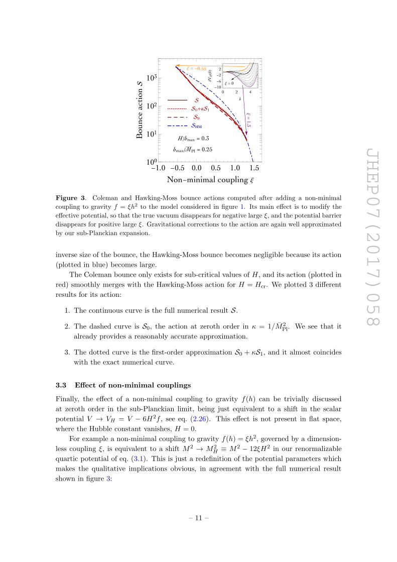
Figure 3. Coleman and Hawking-Moss bounce actions computed after adding a non-minimal

coupling to gravity f = ξh2 to the model considered in figure 1. Its main effect is to modify the

effective potential, so that the true vacuum disappears for negative large ξ, and the potential barrier

disappears for positive large ξ. Gravitational corrections to the action are again well approximated

by our sub-Planckian expansion.

inverse size of the bounce, the Hawking-Moss bounce becomes negligible because its action

(plotted in blue) becomes large.

The Coleman bounce only exists for sub-critical values of H, and its action (plotted in

red) smoothly merges with the Hawking-Moss action for H = Hcr. We plotted 3 different

results for its action:

1. The continuous curve is the full numerical result S.

2. The dashed curve is S0, the action at zeroth order in κ = 1/M2Pl. We see that it

already provides a reasonably accurate approximation.

3. The dotted curve is the first-order approximation S0 + κS1, and it almost coincides

with the exact numerical curve.

3.3 Effect of non-minimal couplings

Finally, the effect of a non-minimal coupling to gravity f(h) can be trivially discussed

at zeroth order in the sub-Planckian limit, being just equivalent to a shift in the scalar

potential V → VH = V − 6H2f , see eq. (2.26). This effect is not present in flat space,

where the Hubble constant vanishes, H = 0.

For example a non-minimal coupling to gravity f(h) = ξh2, governed by a dimension-

less coupling ξ, is equivalent to a shift M2 → M2H ≡ M2 − 12ξH2 in our renormalizable

quartic potential of eq. (3.1). This is just a redefinition of the potential parameters which

makes the qualitative implications obvious, in agreement with the full numerical result

shown in figure 3:

– 11 –

JHEP07(2017)058

• A positive ξ > 0 reduces M2H < M2 and thereby the potential barrier, decreasing

the actions and increasing the tunnelling rate (see also [23]). The critical value Hcr

depends on ξ, so that by increasing ξ one first violates the condition H < Hcr,

leading to the disappearance of Coleman bounces. A larger ξ leads to M2H < 0, so

that the potential barrier disappears and the false vacuum is classically destabilised:

this corresponds to SHM = 0 in figure 3.

• A negative ξ has the effect of increasing the potential barrier. Ultimately, a too large

negative ξ destabilizes the true vacuum: at this point V (htrue) = V (hmax), such that

the Coleman bounce becomes equal to the Hawking-Moss bounce.

In figure 3 we also depict the full numerical action assuming a mildly sub-Planckian poten-

tial with hmax = 0.25MPl: our sub-Planckian expansion again reproduces the full numerical

result. The above simplicity is lost if Planckian energies are involved; however in such a

case Einstein gravity cannot be trusted.

4 Standard Model vacuum decay during inflation

Finally, we apply our general formalism to the case of physical interest: instability of the

electro-weak SM vacuum during inflation.

The probability per unit time and volume of vacuum decay during inflation can be

estimated on dimensional grounds as d℘/dV dt ∼ H4 exp(−S), where S is the action of

the relevant bounce configuration. The total probability of vacuum decay during infla-

tion then is ℘ ∼ TL3H4 exp(−S), corresponding to a total time T ∼ N/H and volume

L3 ∼ H−3 exp(3N), such that ℘ ∼ exp(3N − S). Therefore, a small ‘probability’ ℘ ∼ 1 of

vacuum tunnelling during inflation needs a bounce action S >∼ 3N .9 The horizon of the

visible universe corresponds to a minimal number of N ∼ 60 e-foldings of inflation.

The computation of the bounce actions S in the SM case needs to take into account

the peculiar features of the SM Higgs potential, which is nearly scale-invariant and can be

approximated as

V (h) ≈ λ(h)h4

4≈ −b ln

(h2

h2cr√e

)h4

4, (4.1)

where the running Higgs quartic can turn negative, λ(h) < 0, at large field values. This

happens for the present best-fit values of Mt, Mh and α3, that lead to hcr = 5×1010 GeV [18,

33, 34]. The β-function of λ around hcr can be approximated as b ≈ 0.15/(4π)2.

Furthermore, we add a nonminimal coupling of the Higgs field to gravity f(h) = ξHh2,

such that the effective potential of eq. (2.19) relevant in the sub-Planckian limit is

VH = V − 12ξHH2h

2

2. (4.2)

Finally, we assume that inflation can be approximated as an extra constant term V0 in

the potential. A possible extra quartic scalar coupling of the inflaton to the Higgs would

9Evading this bound trough anthropic selection would need a very special landscape of unstable vacua

with no low-scale inflation.

– 12 –

JHEP07(2017)058

manifest itself as an extra contribution to the effective Higgs mass term in eq. (4.2), which

is equivalent to a modified effective ξH .

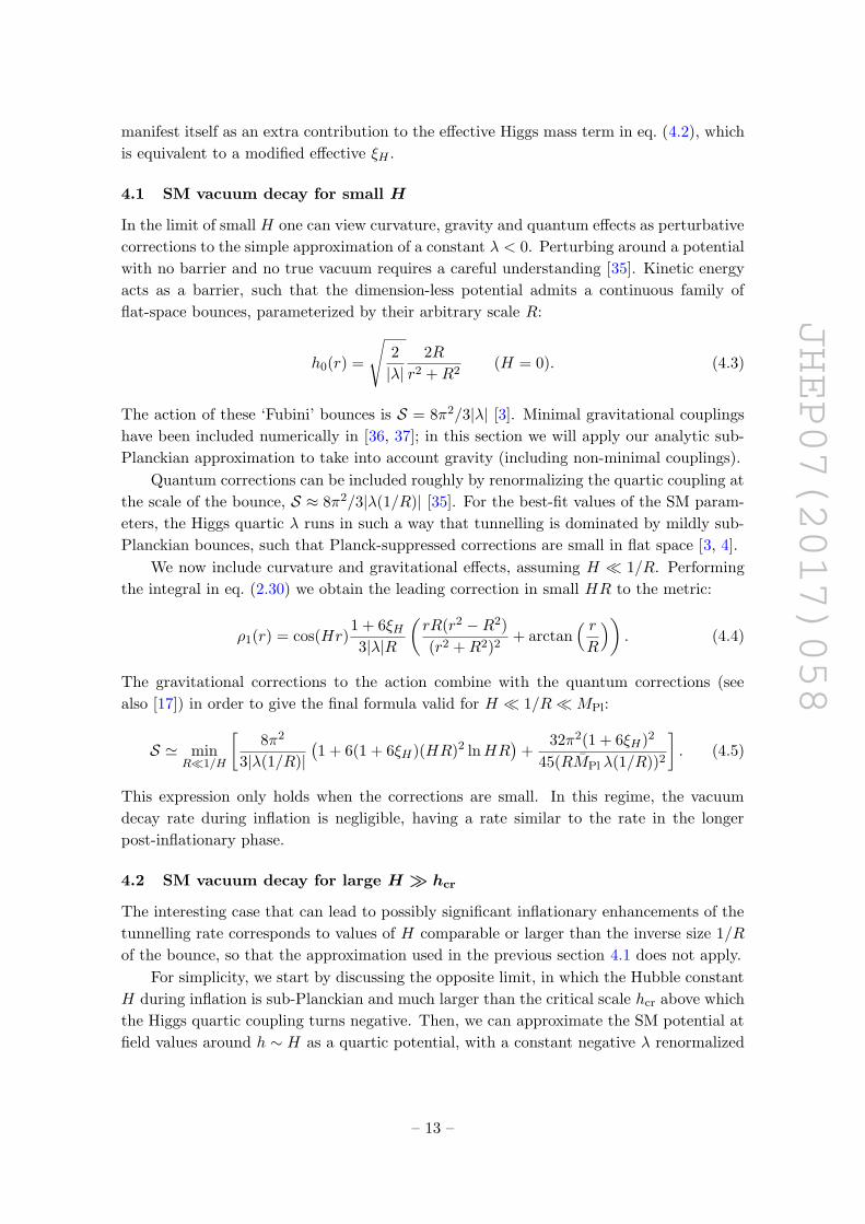
4.1 SM vacuum decay for small H

In the limit of small H one can view curvature, gravity and quantum effects as perturbative

corrections to the simple approximation of a constant λ < 0. Perturbing around a potential

with no barrier and no true vacuum requires a careful understanding [35]. Kinetic energy

acts as a barrier, such that the dimension-less potential admits a continuous family of

flat-space bounces, parameterized by their arbitrary scale R:

h0(r) =

√2

|λ|2R

r2 +R2(H = 0). (4.3)

The action of these ‘Fubini’ bounces is S = 8π2/3|λ| [3]. Minimal gravitational couplings

have been included numerically in [36, 37]; in this section we will apply our analytic sub-

Planckian approximation to take into account gravity (including non-minimal couplings).

Quantum corrections can be included roughly by renormalizing the quartic coupling at

the scale of the bounce, S ≈ 8π2/3|λ(1/R)| [35]. For the best-fit values of the SM param-

eters, the Higgs quartic λ runs in such a way that tunnelling is dominated by mildly sub-

Planckian bounces, such that Planck-suppressed corrections are small in flat space [3, 4].

We now include curvature and gravitational effects, assuming H 1/R. Performing

the integral in eq. (2.30) we obtain the leading correction in small HR to the metric:

ρ1(r) = cos(Hr)1 + 6ξH3|λ|R

(rR(r2 −R2)

(r2 +R2)2+ arctan

( rR

)). (4.4)

The gravitational corrections to the action combine with the quantum corrections (see

also [17]) in order to give the final formula valid for H 1/RMPl:

S ' minR1/H

[8π2

3|λ(1/R)|(1 + 6(1 + 6ξH)(HR)2 lnHR

)+

32π2(1 + 6ξH)2

45(RMPl λ(1/R))2

]. (4.5)

This expression only holds when the corrections are small. In this regime, the vacuum

decay rate during inflation is negligible, having a rate similar to the rate in the longer

post-inflationary phase.

4.2 SM vacuum decay for large H hcr

The interesting case that can lead to possibly significant inflationary enhancements of the

tunnelling rate corresponds to values of H comparable or larger than the inverse size 1/R

of the bounce, so that the approximation used in the previous section 4.1 does not apply.

For simplicity, we start by discussing the opposite limit, in which the Hubble constant

H during inflation is sub-Planckian and much larger than the critical scale hcr above which

the Higgs quartic coupling turns negative. Then, we can approximate the SM potential at

field values around h ∼ H as a quartic potential, with a constant negative λ renormalized

– 13 –

JHEP07(2017)058

around H. Adding the non-minimal coupling to gravity f(h) = ξHh2 gives the effective

potential relevant in the sub-Planckian limit:

δVH = −12ξHH2h

2

2+ λ

h4

4. (4.6)

Scale invariance is broken by the de Sitter background with Hubble constant H, so

that the bounce action can only depend on the dimensionless parameters ξH and λ.

By performing the field redefinition h(r) → αh(r), where α is a constant, one obtains

S(ξH , λ) = α2S(ξH , α2λ) which implies S ∝ 1/λ. Therefore, we only need to compute S

as function of ξH .

A potential barrier exists for ξH < 0: then hmax = H√

12ξH/λ and Hawking-Moss

bounces have action SHM = −96π2ξ2H/λ.

According to the argument in section 3.1, the critical value of H that controls the

existence of Coleman bounces is Hcr =√−V (2)(hmax)/2. For the potential of eq. (4.6) this

means H/Hcr = 1/√−6ξH , so that H = Hcr for ξH = −1/6. As discussed in section 3.1,

Coleman bounces exist for H < Hcr or H > Hcr depending on the sign of the higher-

order coefficient ∆ defined in eq. (3.5). In the present case ∆ ∝ −λ(1 + 6ξH), with a

positive proportionality constant. This potential behaves in an unusual way: ∆ vanishes

at the critical value ξH = −1/6, for which Hawking-Moss bounces have the same action

S = −8π2/3λ as flat-space Fubini bounces. Flat-space bounces are relevant because the

action is Weyl invariant for ξH = −1/6, such that de Sitter space is conformally equivalent

to flat space. Indeed, the Weyl-transformed eq. (2.27) reduces to h′′0+3h′0/r = λh30, satisfied

by Fubini bounces h0 =√

2/|λ|2R/(R2 + r2), where R is an arbitrary constant. By Weyl-

rescaling them back to the original field h0 and coordinate r we obtain the Coleman bounce

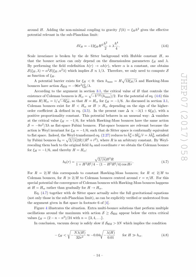
for ξH = −1/6, and thereby H = Hcr:

h0(r) =

√2/|λ|H2R

1 +H2R2/4− (1−H2R2/4) cosHr. (4.7)

For R = 2/H this corresponds to constant Hawking-Moss bounces; for R 2/H to

Coleman bounces, for R 2/H to Coleman bounces centred around r = π/H. For this

special potential the convergence of Coleman bounces with Hawking-Moss bounces happens

at H = Hcr rather than gradually for H → Hcr.

Eq. (4.7) together with de Sitter space actually solve the full gravitational equations

(not only those in the sub-Planckian limit), as can be explicitly verified or understood from

the argument given in flat space in footnote 6 of [4].

Figure 4 illustrates the situation. Extra multi-bounce solutions that perform multiple

oscillations around the maximum with action S ≥ SHM appear below the extra critical

values ξH = (2− n− n2)/24 with n = 3, 4, . . ..In conclusion, vacuum decay is safely slow if SHM > 3N which implies the condition

− ξH <

√−Nλ(H)

32π2≈ −0.04

√−λ(H)

0.01for H hcr. (4.8)

– 14 –

JHEP07(2017)058

- - - -

- ξ

-λ

/

ξ=-/

ξ=-/ξ

=-/

≫

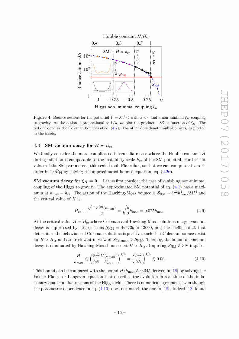
Figure 4. Bounce actions for the potential V = λh4/4 with λ < 0 and a non-minimal ξH coupling

to gravity. As the action is proportional to 1/λ, we plot the product −λS as function of ξH . The

red dot denotes the Coleman bounces of eq. (4.7). The other dots denote multi-bounces, as plotted

in the insets.

4.3 SM vacuum decay for H ∼ hcr

We finally consider the more complicated intermediate case where the Hubble constant H

during inflation is comparable to the instability scale hcr of the SM potential. For best-fit

values of the SM parameters, this scale is sub-Planckian, so that we can compute at zeroth

order in 1/MPl by solving the approximated bounce equation, eq. (2.26).

SM vacuum decay for ξH = 0. Let us first consider the case of vanishing non-minimal

coupling of the Higgs to gravity. The approximated SM potential of eq. (4.1) has a maxi-

mum at hmax = hcr. The action of the Hawking-Moss bounce is SHM = bπ2h4max/3H4 and

the critical value of H is

Hcr ≡√−V (2)(hmax)

2=

√b

2hmax = 0.025hmax. (4.9)

At the critical value H = Hcr where Coleman and Hawking-Moss solutions merge, vacuum

decay is suppressed by large actions SHM = 4π2/3b ≈ 13000, and the coefficient ∆ that

determines the behaviour of Coleman solutions is positive, such that Coleman bounces exist

for H > Hcr and are irrelevant in view of SColeman > SHM. Thereby, the bound on vacuum

decay is dominated by Hawking-Moss bounces at H > Hcr. Imposing SHM <∼ 3N implies

H

hmax

<∼(

8π2

9N

V (hmax)

h4max

)1/4

=

(bπ2

9N

)1/4

<∼ 0.06. (4.10)

This bound can be compared with the bound H/hmax <∼ 0.045 derived in [18] by solving the

Fokker-Planck or Langevin equation that describes the evolution in real time of the infla-

tionary quantum fluctuations of the Higgs field. There is numerical agreement, even though

the parametric dependence in eq. (4.10) does not match the one in [18]. Indeed [18] found

– 15 –

JHEP07(2017)058

- - - - -

-

- ξ

/

< > >

> >>

=

ξ =-/

ξ =-

<

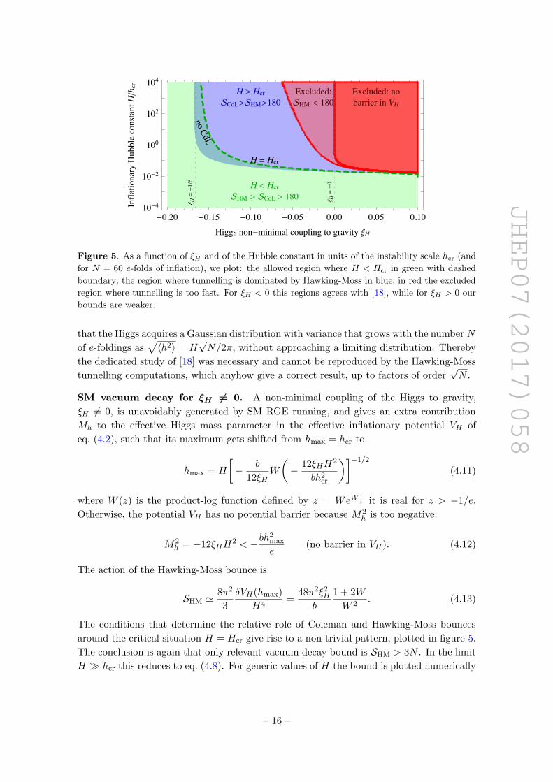
Figure 5. As a function of ξH and of the Hubble constant in units of the instability scale hcr (and

for N = 60 e-folds of inflation), we plot: the allowed region where H < Hcr in green with dashed

boundary; the region where tunnelling is dominated by Hawking-Moss in blue; in red the excluded

region where tunnelling is too fast. For ξH < 0 this regions agrees with [18], while for ξH > 0 our

bounds are weaker.

that the Higgs acquires a Gaussian distribution with variance that grows with the number N

of e-foldings as√〈h2〉 = H

√N/2π, without approaching a limiting distribution. Thereby

the dedicated study of [18] was necessary and cannot be reproduced by the Hawking-Moss

tunnelling computations, which anyhow give a correct result, up to factors of order√N .

SM vacuum decay for ξH 6= 0. A non-minimal coupling of the Higgs to gravity,

ξH 6= 0, is unavoidably generated by SM RGE running, and gives an extra contribution

Mh to the effective Higgs mass parameter in the effective inflationary potential VH of

eq. (4.2), such that its maximum gets shifted from hmax = hcr to

hmax = H

[− b

12ξHW

(− 12ξHH

2

bh2cr

)]−1/2(4.11)

where W (z) is the product-log function defined by z = WeW : it is real for z > −1/e.

Otherwise, the potential VH has no potential barrier because M2h is too negative:

M2h = −12ξHH

2 < −bh2max

e(no barrier in VH). (4.12)

The action of the Hawking-Moss bounce is

SHM '8π2

3

δVH(hmax)

H4=

48π2ξ2Hb

1 + 2W

W 2. (4.13)

The conditions that determine the relative role of Coleman and Hawking-Moss bounces

around the critical situation H = Hcr give rise to a non-trivial pattern, plotted in figure 5.

The conclusion is again that only relevant vacuum decay bound is SHM > 3N . In the limit

H hcr this reduces to eq. (4.8). For generic values of H the bound is plotted numerically

– 16 –

JHEP07(2017)058

in figure 5, where the red region is excluded because inflationary vacuum decay is too fast.

For ξH < 0 such bound agrees with the corresponding result of [18]. Indeed [18] found

that a positive M2h > 0 limits the Higgs fluctuations which, after a few e-foldings, converge

towards a limiting distribution, well described by the Hawking-Moss transition. On the

other hand, for M2h ≤ 0 (ξH ≥ 0) the Higgs fluctuations grow with N (as

√N for M2

h = 0,

and exponentially for M2h < 0), so that the detailed dynamical study of [18] is needed. Nev-

ertheless, for ξH > 0, the bound SHM > 3N , is almost numerically equivalent to the simpler

bound on M2h in eq. (4.12) that guarantees that VH has a potential barrier, which reads

H

hmax

<∼(

b

12eξH

)1/2

<∼0.005√ξH

. (4.14)

figure 5 shows that this bound is weaker than the bound of [18]. A Langevin simulation

performed along the lines of [18] agrees with our bound, while [18] made a simplifying ap-

proximation (‘neglecting the small Higgs quartic coupling’) which is not accurate around

the bound at ξH > 0.

5 Conclusions

In section 2 we developed a simplified formalism for computing vacuum decay from a de

Sitter space with Hubble constant H, assuming that both H and the mass scale of the

scalar potential are sub-Planckian. This is not a limitation, given that otherwise Einstein

gravity cannot anyhow be trusted. In this approximation, the bounce action is obtained as

a power series in 1/MPl, and a non-minimal scalar coupling to gravity can be reabsorbed

in an effective scalar potential, see eq. (2.19).

In section 3 we considered a renormalizable single-field potential. We verified that

our expansion reproduces full numerical result. Furthermore we found that, increasing H,

the flat-space Coleman bounce continuously deforms into the Hawking-Moss bounce. Only

the Hawking-Moss bounce exists above a critical value of the Hubble constant, equal to

H2cr = −V (2)(hmax)/4. For H < Hcr the Coleman bounce appears and dominates vacuum

decay, having a smaller action than the Hawking-Moss bounce. For smaller values of H

extra bounces that oscillate around the top of the barrier appear, but they never dominate

the path-integral. In the flat space limit H → 0 they reduce to the infinite series of

multi-bounce solutions.

In section 4 we studied quantum tunnelling of the electroweak vacuum during inflation,

assuming that the SM Higgs potential is unstable at large field values, as happens for

present central values of the SM parameters. Coleman bounces are still connected to

Hawking-Moss bounces, altough the fact that the SM potential has a negative quartic at

large field values and is quasi-scale-invariant makes their relation different. We exhibit

a limit where they are conformally equivalent. Anyhow we found that only Hawking-

Moss bounces imply a significant bound on vacuum decay during inflation. If the minimal

coupling of the Higgs to gravity is negative, ξH < 0, our tunnelling computation confirms

previous upper bounds on H obtained from statistical simulations (needed to address other

cosmological issues). If ξH > 0 we find weaker bounds, and explain why the approximation

made in earlier works [18] is not accurate.

– 17 –

JHEP07(2017)058

Acknowledgments

We thank G. D’Amico, J.R. Espinosa, A. Rajantie, M. Schwartz and S.M. Sibiryakov for

useful discussions. This work was supported by the ERC grant NEO-NAT. The work of

A. Katsis is co-financed by the European Union (European Social Fund — ESF) and Greek

national funds through the action “Strengthening Human Resources Research Potential

via Doctorate Research” of State Scholarships Foundation (IKY), in the framework of

the Operational Programme “Human Resources Development Program, Education and

Lifelong Learning” of the National Strategic Reference Framework (NSRF) 2014–2020.

Open Access. This article is distributed under the terms of the Creative Commons

Attribution License (CC-BY 4.0), which permits any use, distribution and reproduction in

any medium, provided the original author(s) and source are credited.

References

[1] S.R. Coleman, The Fate of the False Vacuum. 1. Semiclassical Theory Phys. Rev. D 15

(1977) 2929 [Erratum ibid. D 16 (1977) 1248] [INSPIRE].

[2] S.R. Coleman and F. De Luccia, Gravitational Effects on and of Vacuum Decay, Phys. Rev.

D 21 (1980) 3305 [INSPIRE].

[3] G. Isidori, V.S. Rychkov, A. Strumia and N. Tetradis, Gravitational corrections to standard

model vacuum decay, Phys. Rev. D 77 (2008) 025034 [arXiv:0712.0242] [INSPIRE].

[4] A. Salvio, A. Strumia, N. Tetradis and A. Urbano, On gravitational and thermal corrections

to vacuum decay, JHEP 09 (2016) 054 [arXiv:1608.02555] [INSPIRE].

[5] G.W. Gibbons and S.W. Hawking, Cosmological Event Horizons, Thermodynamics, and

Particle Creation, Phys. Rev. D 15 (1977) 2738 [INSPIRE].

[6] S.W. Hawking and I.G. Moss, Supercooled Phase Transitions in the Very Early Universe,

Phys. Lett. B 110 (1982) 35 [INSPIRE].

[7] J.R. Espinosa, G.F. Giudice and A. Riotto, Cosmological implications of the Higgs mass

measurement, JCAP 05 (2008) 002 [arXiv:0710.2484] [INSPIRE].

[8] A. Kobakhidze and A. Spencer-Smith, Electroweak Vacuum (In)Stability in an Inflationary

Universe, Phys. Lett. B 722 (2013) 130 [arXiv:1301.2846] [INSPIRE].

[9] A. Kobakhidze and A. Spencer-Smith, The Higgs vacuum is unstable, arXiv:1404.4709

[INSPIRE].

[10] M. Fairbairn and R. Hogan, Electroweak Vacuum Stability in light of BICEP2, Phys. Rev.

Lett. 112 (2014) 201801 [arXiv:1403.6786] [INSPIRE].

[11] K. Enqvist, T. Meriniemi and S. Nurmi, Higgs Dynamics during Inflation, JCAP 07 (2014)

025 [arXiv:1404.3699] [INSPIRE].

[12] K. Kamada, Inflationary cosmology and the standard model Higgs with a small Hubble

induced mass, Phys. Lett. B 742 (2015) 126 [arXiv:1409.5078] [INSPIRE].

[13] A. Hook, J. Kearney, B. Shakya and K.M. Zurek, Probable or Improbable Universe?

Correlating Electroweak Vacuum Instability with the Scale of Inflation, JHEP 01 (2015) 061

[arXiv:1404.5953] [INSPIRE].

– 18 –

JHEP07(2017)058

[14] M. Herranen, T. Markkanen, S. Nurmi and A. Rajantie, Spacetime curvature and the Higgs

stability during inflation, Phys. Rev. Lett. 113 (2014) 211102 [arXiv:1407.3141] [INSPIRE].

[15] J. Kearney, H. Yoo and K.M. Zurek, Is a Higgs Vacuum Instability Fatal for High-Scale

Inflation?, Phys. Rev. D 91 (2015) 123537 [arXiv:1503.05193] [INSPIRE].

[16] W.E. East, J. Kearney, B. Shakya, H. Yoo and K.M. Zurek, Spacetime Dynamics of a Higgs

Vacuum Instability During Inflation, Phys. Rev. D 95 (2017) 023526 [arXiv:1607.00381]

[INSPIRE].

[17] A. Shkerin and S. Sibiryakov, On stability of electroweak vacuum during inflation, Phys. Lett.

B 746 (2015) 257 [arXiv:1503.02586] [INSPIRE].

[18] J.R. Espinosa et al., The cosmological Higgstory of the vacuum instability, JHEP 09 (2015)

174 [arXiv:1505.04825] [INSPIRE].

[19] K. Kohri and H. Matsui, Higgs vacuum metastability in primordial inflation, preheating and

reheating, Phys. Rev. D 94 (2016) 103509 [arXiv:1602.02100] [INSPIRE].

[20] A. Rajantie and S. Stopyra, Standard Model vacuum decay with gravity, Phys. Rev. D 95

(2017) 025008 [arXiv:1606.00849] [INSPIRE].

[21] K. Enqvist, M. Karciauskas, O. Lebedev, S. Rusak and M. Zatta, Postinflationary vacuum

instability and Higgs-inflaton couplings, JCAP 11 (2016) 025 [arXiv:1608.08848] [INSPIRE].

[22] Y. Ema, M. Karciauskas, O. Lebedev and M. Zatta, Early Universe Higgs dynamics in the

presence of the Higgs-inflaton and non-minimal Higgs-gravity couplings, JCAP 06 (2017) 054

[arXiv:1703.04681] [INSPIRE].

[23] O. Czerwinska, Z. Lalak, M. Lewicki and P. Olszewski, The impact of non-minimally coupled

gravity on vacuum stability, JHEP 10 (2016) 004 [arXiv:1606.07808] [INSPIRE].

[24] S.K. Blau, E.I. Guendelman and A.H. Guth, The Dynamics of False Vacuum Bubbles, Phys.

Rev. D 35 (1987) 1747.

[25] U. Nucamendi and M. Salgado, Scalar hairy black holes and solitons in asymptotically flat

space-times, Phys. Rev. D 68 (2003) 044026 [gr-qc/0301062] [INSPIRE].

[26] J. Callan and S.R. Coleman, The Fate of the False Vacuum. 2. First Quantum Corrections,

Phys. Rev. D 16 (1977) 1762 [INSPIRE].

[27] A. Andreassen, D. Farhi, W. Frost and M.D. Schwartz, Precision decay rate calculations in

quantum field theory, Phys. Rev. D 95 (2017) 085011 [arXiv:1604.06090] [INSPIRE].

[28] Planck collaboration, P.A.R. Ade et al., Planck 2015 results. XX. Constraints on inflation,

Astron. Astrophys. 594 (2016) A20 [arXiv:1502.02114] [INSPIRE].

[29] B.-H. Lee and W. Lee, Vacuum bubbles in a de Sitter background and black hole pair

creation, Class. Quant. Grav. 26 (2009) 225002 [arXiv:0809.4907] [INSPIRE].

[30] V. Balek and M. Demetrian, Euclidean action for vacuum decay in a de Sitter universe,

Phys. Rev. D 71 (2005) 023512 [gr-qc/0409001] [INSPIRE].

[31] L.G. Jensen and P.J. Steinhardt, Bubble Nucleation and the Coleman-Weinberg Model, Nucl.

Phys. B 237 (1984) 176 [INSPIRE].

[32] J.C. Hackworth and E.J. Weinberg, Oscillating bounce solutions and vacuum tunneling in

de Sitter spacetime, Phys. Rev. D 71 (2005) 044014 [hep-th/0410142] [INSPIRE].

– 19 –

JHEP07(2017)058

[33] J. Elias-Miro, J.R. Espinosa, G.F. Giudice, G. Isidori, A. Riotto and A. Strumia, Higgs mass

implications on the stability of the electroweak vacuum, Phys. Lett. B 709 (2012) 222

[arXiv:1112.3022] [INSPIRE].

[34] D. Buttazzo et al., Investigating the near-criticality of the Higgs boson, JHEP 12 (2013) 089

[arXiv:1307.3536] [INSPIRE].

[35] G. Isidori, G. Ridolfi and A. Strumia, On the metastability of the standard model vacuum,

Nucl. Phys. B 609 (2001) 387 [hep-ph/0104016] [INSPIRE].

[36] B.-H. Lee, W. Lee, C. Oh, D. Ro and D.-h. Yeom, Fubini instantons in curved space, JHEP

06 (2013) 003 [arXiv:1204.1521] [INSPIRE].

[37] B.-H. Lee, W. Lee, D. Ro and D.-h. Yeom, Oscillating Fubini instantons in curved space,

Phys. Rev. D 91 (2015) 124044 [arXiv:1409.3935] [INSPIRE].

– 20 –