Local Ecological Footprinting Toolwww.left.ox.ac.uk

Puntarenas

Costa Rica site 3587

This report contains a series of maps and tables identifying parts of the landscape whichare relatively more important because of the ecological features found there.

Date 11 Nov 2016, 7:01 PMSubmitter leftsupport@zoo.ox.ac.uk

1 Introduction

The Local Ecological Footprinting Tool (LEFT)was developed to provide a simple-to-use tool for industriesand landowners who have to make quick preliminary decisions about land-use change, and to assist inminimising the environmental impact of their operations.

The tool processes a series of high-quality open-access environmental datasets using standardised algo-rithms to produce maps at 30m resolution of land cover class, number of globally threatened terrestrialvertebrate and plant species, biodiversity of terrestrial vertebrates and plants, habitat intactness, wetlandhabitat connectivity, number of migratory species, and vegetation resilience. These results are aggregatedin a single summary map showing the pattern of relative ecological value.

This report briefly describes the methods and datasets used to generate the maps for the specified areaof interest. Further details on the modelling approach, datasets, and choice of ecological variables canbe found in Willis et al., (2012; 2014; 2015) and Long et al., (2016 – in press)

Please note that this report was generated automatically. If you have any questions about LEFT or thisoutput, please email support@left.zoo.ox.ac.uk.

Area of Interest

The specified area of interest for this analysis has the following bounding co-ordinates:

Latitude: 9.60°N to 10.39°NLongitude: 85.40°W to 84.36°W

2

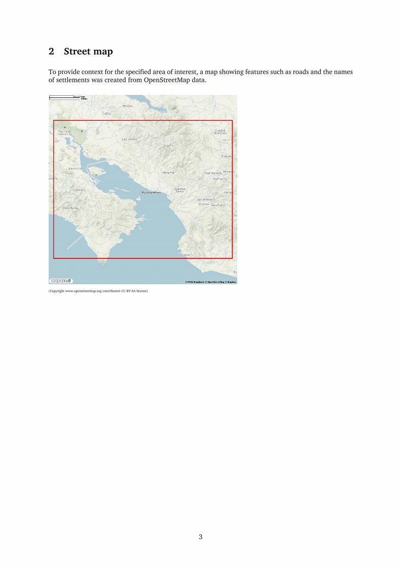
2 Street map

To provide context for the specified area of interest, a map showing features such as roads and the namesof settlements was created from OpenStreetMap data.

(Copyright www.openstreetmap.org contributors CC BY-SA license)

3

3 Land cover

A map showing land cover in the year 2010 was derived from the GlobeLand30 data set (CopyrightNational Geomatics Center of China, DOI:10.11769/GlobeLand30.2010.db). Pixels were classified toland cover categories from multispectral Landsat and HJ-1 images, plus auxiliary data. In isolated areaswithout GlobeLand30 coverage, GlobCover 2009 land cover was used instead (Copyright ESA GlobCoverProject, led by MEDIAS-France). OpenStreetMap land polygons were used to mask sea pixels.

Longitude

Latit

ude

Land cover map of the specified area of interest. Spatial resolution is 1 arcsec, or approximately 30metres.

4

4 Ecoregions

The WWF Terrestrial Ecoregion Classification (Olson et al. 2001) was used to identify the ecoregion(s)containing the specified area of interest. Relevant georeferenced biodiversity records were retrieved forthis area from the Global Biodiversity Information Facility (GBIF, www.gbif.org). In addition, speciesoccurrence data in the same ecoregions, up to a 3-degree buffer, were obtained to ensure a maximumnumber of records for modelling.

Longitude

Latit

ude

Terrestrial Ecoregions in the specified area of interest and in a surrounding 3-degree buffer.

5

5 Species occurrence data

The map below indicates the distribution of the georeferenced GBIF species occurrence records of am-phibians, reptiles, birds, mammals, and plants for the specified area of interest plus a 3-degree bufferzone. Any duplicate records (of the same species recorded more than once in the same location) wereremoved. Text files containing these records are available in the output zip file (see Appendix 1: OutputFiles).

Taxon Number of species Number of Records ColourAmphibians 185 1766Reptiles 259 2028Mammals 206 1653Birds 836 33960Plants 8697 46117Total 10183 85524

The table above indicates the number of species occurence records retrieved from GBIF for the specifiedarea of interest plus buffer zone. Circles on the map are colour coded by taxonomic group (Amphibians– pink; Reptiles – light blue; Mammals – orange; Birds – dark blue; Plants – green).

6

6 Spatial pattern of biodiversity

The species records retrieved from GBIF (above) were combined with environmental covariates to expressthe pattern of biodiversity (beta-diversity, i.e. spatial turnover in species) across the area of interest. To dothis, a Generalised Dissimilarity Model (GDM; Ferrier et al 2002) was run. The environmental covariatesused in the model were annual mean temperature, annual mean precipitation, temperature seasonality,precipitation seasonality (Hijmans et al 2005), soil nitrogen, soil water holding capacity (Land and WaterDevelopment Division, FAO 2003), and land cover class (GlobCover 2009).

Longitude

Latit

ude

Beta-diversity in the specified area of interest. High values of beta-diversity (in red) represent greaterspatial heterogenity in the set of species present compared to other parts of the area of interest. Lowbeta-diversity values (in blue) indicate a relatively homogeneous set of species.

7

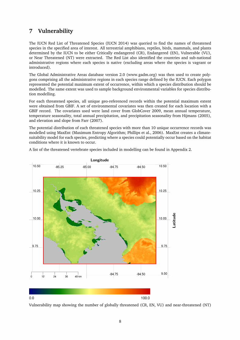
7 Vulnerability

The IUCN Red List of Threatened Species (IUCN 2014) was queried to find the names of threatenedspecies in the specified area of interest. All terrestrial amphibians, reptiles, birds, mammals, and plantsdetermined by the IUCN to be either Critically endangered (CR), Endangered (EN), Vulnerable (VU),or Near Threatened (NT) were extracted. The Red List also identified the countries and sub-nationaladministrative regions where each species is native (excluding areas where the species is vagrant orintroduced).

The Global Administrative Areas database version 2.0 (www.gadm.org) was then used to create poly-gons comprising all the administrative regions in each species range defined by the IUCN. Each polygonrepresented the potential maximum extent of occurrence, within which a species distribution should bemodelled. The same extent was used to sample background environmental variables for species distribu-tion modelling.

For each threatened species, all unique geo-referenced records within the potential maximum extentwere obtained from GBIF. A set of environmental covariates was then created for each location with aGBIF record. The covariates used were land cover from GlobCover 2009, mean annual temperature,temperature seasonality, total annual precipitation, and precipitation seasonality from Hijmans (2005),and elevation and slope from Farr (2007).

The potential distribution of each threatened species with more than 10 unique occurrence records wasmodelled using MaxEnt (Maximum Entropy Algorithm; Phillips et al., 2006). MaxEnt creates a climate-suitability model for each species, predicting where a species could potentially occur based on the habitatconditions where it is known to occur.

A list of the threatened vertebrate species included in modelling can be found in Appendix 2.

Longitude

Latit

ude

Vulnerability map showing the number of globally threatened (CR, EN, VU) and near-threatened (NT)

8

terrestrial vertebrates and plants estimated to occur in the specified area of interest. Red indicates wherethe landscape contains the highest number of threatened species. See Appendix 2 for a list of speciesnames.

9

8 Intactness

To identify patches of intact habitat in the specified area of interest, the land cover map described abovewas reclassified. Pixels in the urban/artificial, bare ground, and snow/ice categories were omitted fromconsideration. Every remaining pixel was assigned to a group of neighbouring pixels with the same landcover class, and the area of each group in hectares was calculated. In the resulting map those areas witha greater intact patch size are less fragmented, and carry a higher ecological value.

Longitude

Latit

ude

Intactness map. Values express the size of the land cover patch to which each pixel belongs (ln(patcharea in ha) x 10). Urban, bare, and snow pixels were assigned an intactness value of 0. Resolution of thedata is 1 arcsec, or about 30m.

10

9 Connectivity: Migratory species

Habitat connectivity across a landscape is usually achieved through wetland corridors and/or other mi-gratory routes. To remotely characterise important migratory routes, the Global Register of MigratorySpecies (GROMS; www.groms.de; Riede 2004) was queried. This database provided both a list of 4,430migratory vertebrate species (terrestrial birds and mammals) and digital maps describing the migratoryroutes for >1,000 of those species. Grids for all species shown to have a migratory route across the areaof interest were added together to yield an estimate of migratory species density.

Longitude

Latit

ude

Number of migration corridors overlapping the specified area of interest. A list of the migratory speciespotentially crossing this area can be found in Appendix 3.

11

10 Connectivity: Wetlands

A measure of wetland dispersal corridors across the specified area of interest was derived from the landcover map described previously. Pixels within 100 metres of water bodies were identified. Those bufferzones, along with pixels classed as Inland water or Wetland, were assigned a high ecological value of 1.All other land pixels were given a value of 0.

Longitude

Latit

ude

Wetland connectivity showing areas of open water, permanent wetland, or within 100m of water. Theresolution of the data is 1 arcsec, approximately 30m.

12

11 Resilience

The resilience of vegetation to climate perturbations was estimated usingmonthly time series of EnhancedVegetation Index (EVI) and three climate variables. A PCA regression was performed between EVI andair temperature, the ratio of actual to potential evapotranspiration, and cloud cover for the period 2000-2013. This identified the months when EVI is related to climate drivers and measured the strength ofthat relationship over 14 years.

Next the variability in EVI and in each climate variable was calculated. A measure of sensitivity to eachclimate variable was determined by dividing EVI variability by climate variability, thus measuring howmuch EVI varied per variation in climate (i.e. the nervousness of EVI to climate).

In the resultant resilience map, high values indicate areas where vegetation maintained greenness despitefluctuations in climate. Low resilience values reveal areas where photosynthetic activity changed whenclimate anomalies occurred.

Longitude

Latit

ude

Red indicates regions of greater vegetation resilience to climatic perturbations.

13

12 Summary Ecological Value

In addition to the preceding maps, a summary ecological valuation (SEV) was calculated for the specifiedarea of interest. In this, each of the above layers was standardised into a map of Z-scores. Z-scores werethen added together to show the landscape pattern of each layer on a scale comparable to all the otherlayers. For example, a pixel with the same value as the mean of its layer across the area of interest wouldhave a Z-score of 0, while a pixel one standard deviation above the mean for that layer would have aZ-score of 1, and a pixel one standard deviation below the layer mean would have a Z-score of -1.

Longitude

Latit

ude

Summary ecological value of all LEFT layers in the area of interest. Areas with high SEV are relativelyimportant across several measures of ecological value, while areas with low SEV are relatively less im-portant. The resolution of the data is 1 arcsec, approximately 30m.

14

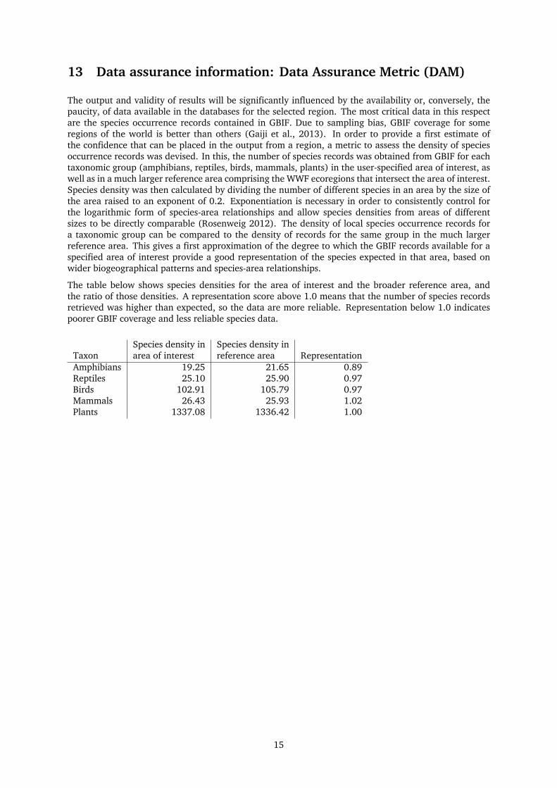
13 Data assurance information: Data Assurance Metric (DAM)

The output and validity of results will be significantly influenced by the availability or, conversely, thepaucity, of data available in the databases for the selected region. The most critical data in this respectare the species occurrence records contained in GBIF. Due to sampling bias, GBIF coverage for someregions of the world is better than others (Gaiji et al., 2013). In order to provide a first estimate ofthe confidence that can be placed in the output from a region, a metric to assess the density of speciesoccurrence records was devised. In this, the number of species records was obtained from GBIF for eachtaxonomic group (amphibians, reptiles, birds, mammals, plants) in the user-specified area of interest, aswell as in a much larger reference area comprising the WWF ecoregions that intersect the area of interest.Species density was then calculated by dividing the number of different species in an area by the size ofthe area raised to an exponent of 0.2. Exponentiation is necessary in order to consistently control forthe logarithmic form of species-area relationships and allow species densities from areas of differentsizes to be directly comparable (Rosenweig 2012). The density of local species occurrence records fora taxonomic group can be compared to the density of records for the same group in the much largerreference area. This gives a first approximation of the degree to which the GBIF records available for aspecified area of interest provide a good representation of the species expected in that area, based onwider biogeographical patterns and species-area relationships.

The table below shows species densities for the area of interest and the broader reference area, andthe ratio of those densities. A representation score above 1.0 means that the number of species recordsretrieved was higher than expected, so the data are more reliable. Representation below 1.0 indicatespoorer GBIF coverage and less reliable species data.

TaxonSpecies density inarea of interest

Species density inreference area Representation

Amphibians 19.25 21.65 0.89Reptiles 25.10 25.90 0.97Birds 102.91 105.79 0.97Mammals 26.43 25.93 1.02Plants 1337.08 1336.42 1.00

15

14 Data assurance information: Compared to other regions (COAM)

To appreciate the importance of the ecological values obtained for the specified area of interest relative toother regions, a 'compared to other areas metric' (COAM) was calculated. This metric used the polygonsof the WWF Terrestrial Ecoregion Classification (Olson et al, 2001) to identify zones ecologically similarto the area of interest. Zonal statistics were then used to assess the importance of each LEFT layer relativeto the same measure over the entire ecoregion. For each layer, the difference in standard scores betweenthe area of interest and the broader ecoregions is presented in the following chart. This shows whethera study area is relatively more or less ecologically valuable than other regions with similar biogeographiccharacterisitics.

List of ecoregions which intersect the region of interest:

Central American dry forests; Costa Rican seasonalmoist forests; Isthmian-Atlanticmoist forests; Isthmian-Pacific moist forests; Southern Mesoamerican Pacific mangroves; Talamancan montane forests

Layer Min Max Mean SD Ref. Mean Ref. SDBeta-diversity 0.61 0.75 0.64 0.03 0.74 0.07Vulnerability 0.00 94.00 48.79 14.96 46.29 4.01Intactness 0.00 168.00 122.59 49.06 41.40 51.28Migratory 24.00 93.00 82.31 11.85 81.63 9.87Wetland 0.00 1.00 0.04 0.19 0.06 0.22Resilience 0.63 0.93 0.82 0.04 0.81 0.05

Table and chart indicating the importance of the area of interest relative to the reference region for eachlayer (standard scores +/- uncertainty in standard scores). If a layer has a positive standard score thenthe area of interest is more important than the reference region; a layer with a negative standard scoreis less important in the study area than in the reference region.

16

References

Ferrier S, Drielsma M et al. (2002) Extended statistical approaches to modelling spatial pattern in bio-diversity in northeast New South Wales. II. Community-level modelling. Biodiversity and Conservation.11: 2309-2338

Hijmans RJ, Cameron SE et al. (2005) Very high resolution interpolated climate surfaces for global landareas. International Journal of Climatology. 25: 1965-1978

IUCN (2014) Red list of threatened species, version 2014.1

Land and Water Development Division, FAO, Rome (2003) The digital soil map of the world.

National Geomatics Center of China (2014) 30-meter Global Land Cover Dataset (GlobeLand30).www.globallandcover.com, DOI:10.11769/GlobeLand30.2010.db

Olson DM, Dinerstein E et al. (2001) Terrestrial ecoregions of the world: a new map of life on earth.Bioscience 51: 933-938

Phillips SJ, Anderson RP et al. (2006) Maximum entropy modelling of species geographic distributions.Ecological Modelling 190: 231-259

Riede K (2004) Global register of migratory species: from global to regional scales. Final report of theR&D Project. Bonn, Federal Agency for Nature Conservation

Rosenzweig ML, Donoghue J, Li YM, Yuan C (2010) Estimating Species Density. In Magurran AE andMcGill BJ (eds) Biological Diversity: Frontiers in Measurement and Assessment

Credits

The concept of LEFT was developed by Kathy Willis and Elizabeth Jeffers of the Zoology Department,University of Oxford and Randi Hagemann, Tone Karin Frost, Mathijs Smit, Christian Collin-Hansen, andJurgen Weissenberger from Statoil ASA.

The algorithms in LEFT II were developed by Peter Long, David Benz, Marc Macias Fauria, and Alis-tair Seddon of the Zoology Department, University of Oxford. Spatial data processing for LEFT II wasperformed by Peter Long and David Benz.

Andrew Simpson, David Power, and Mark Slaymaker at the Department of Computer Science, Universityof Oxford developed the service-oriented interoperability framework (sif) middleware used to provideLEFT II as an automatic web-based tool. Richard Smith, of Tessella, and Philip Holland contributed toextending the functionality of the sif plugins in LEFT II.

The development of LEFT and LEFT II was funded by Statoil.

Copyright © 2010-2015

This report (including any attachments) has been supplied for the exclusive use and benefit of the person (or its principal, as the case may be) who made the contract of supply for the report and is subject tothe terms and conditions forming part of that contract. If a third party uses this report for any purpose, it does so at its own risk and the University of Oxford ("the University") accepts no responsibility for anysuch use. Additionally, the University accepts no duty of care to any such third party.

Notwithstanding that use of this report by a third party is not intended or permitted by the University, subject to the following paragraph, the University hereby excludes all liability in connection with any use ofthis report made by a third party (whether in contract, tort (including negligence) or otherwise) to the fullest extent permitted by law, including (without limitation or affecting the generality of the foregoing)in respect of liability for any loss of profits or of contracts, loss of business or of revenues, loss of goodwill or reputation, whether caused directly or indirectly.

Nothing in this disclaimer is intended to limit or exclude any liability which cannot be limited or excluded by law, including for death or personal injury caused by negligence or for fraudulent misrepresentation.

The copyright in this report belongs to the University of Oxford and no express or implied licence is given to any third party to copy or reproduce it or any part without the University's prior written consent.

17

Appendix 1: Output Files

Clicking on the "ZIP" button for this analysis when logged in on the LEFT website will allow you todownload a file named output.zip. This contains:

In the root,A copy of this document: report.pdf

In the folder /data/Folders for each LEFT layer containing a copy of the styled map for that layer presented in this report.The styled maps are in PNG format.

In the folder /data/biodiversity/output/result/Text files for each taxonomic group containing all GBIF records retrieved during this analysis: aves.txt,amphibian.txt, mammalian.txt, reptilian.txt, and plantae.txt

Clicking on the "GeoTIFF ZIP" button for this analysis when logged in on the LEFT website will allow youto download a file named geotiffs.zip. This contains:

In the root,Folders for each of the following LEFT layers: land cover class, beta-diversity, vulnerability, fragmenta-tion, migratory species, wetlands, resilience, and summary ecological value

Each folder contains a single geoTIFF file. This is a copy of the image for that layer subset to the specifiedarea of interest at full spatial resolution (1 arcsec, approximately 30m). Images are either 8-bit or 16-bitdepth. Projection is latitutde/longitude on the WGS1984 datum. These geoTIFF files can be opened withstandard desktop GIS software to perform further analyses.

18

Appendix 2: Vulnerable Species

The IUCN Redlist of Threatened Species (IUCN 2014) includes the following species of terrestrial mam-mals, birds, reptiles, and amphibians that have been modelled to be potentially present in the specifiedarea of interest (NT = Near Threatened, VU = Vulnerable, EN = Endangered, CR = Critically Endan-gered):

Agalychnis annae ( amphibian EN ) (http://en.wikipedia.org/wiki/Agalychnis_annae)Amazilia boucardi ( bird EN ) (http://en.wikipedia.org/wiki/Amazilia_boucardi)Anoura cultrata ( mammal NT ) (http://en.wikipedia.org/wiki/Anoura_cultrata)Aphanotriccus capitalis ( bird VU ) (http://en.wikipedia.org/wiki/Aphanotriccus_capitalis)Ateles geoffroyi ( mammal EN ) (http://en.wikipedia.org/wiki/Ateles_geoffroyi)Atelopus varius ( amphibian CR ) (http://en.wikipedia.org/wiki/Atelopus_varius)Bangsia arcaei ( bird NT ) (http://en.wikipedia.org/wiki/Bangsia_arcaei)Bauerus dubiaquercus ( mammal NT ) (http://en.wikipedia.org/wiki/Bauerus_dubiaquercus)Bolitoglossa alvaradoi ( amphibian EN ) (http://en.wikipedia.org/wiki/Bolitoglossa_alvaradoi)Bolitoglossa lignicolor ( amphibian VU ) (http://en.wikipedia.org/wiki/Bolitoglossa_lignicolor)Bolitoglossa subpalmata ( amphibian EN ) (http://en.wikipedia.org/wiki/Bolitoglossa_subpalmata)Carpodectes antoniae ( bird EN ) (http://en.wikipedia.org/wiki/Carpodectes_antoniae)Cephalopterus glabricollis ( bird VU ) (http://en.wikipedia.org/wiki/Cephalopterus_glabricollis)Chaetura pelagica ( bird NT ) (http://en.wikipedia.org/wiki/Chaetura_pelagica)Chamaepetes unicolor ( bird NT ) (http://en.wikipedia.org/wiki/Chamaepetes_unicolor)Contopus cooperi ( bird NT ) (http://en.wikipedia.org/wiki/Contopus_cooperi)Cotinga ridgwayi ( bird VU ) (http://en.wikipedia.org/wiki/Cotinga_ridgwayi)Craugastor andi ( amphibian CR ) (http://en.wikipedia.org/wiki/Craugastor_andi)Craugastor angelicus ( amphibian CR ) (http://en.wikipedia.org/wiki/Craugastor_angelicus)Craugastor persimilis ( amphibian VU ) (http://en.wikipedia.org/wiki/Craugastor_persimilis)Craugastor podiciferus ( amphibian NT ) (http://en.wikipedia.org/wiki/Craugastor_podiciferus)Craugastor ranoides ( amphibian CR ) (http://en.wikipedia.org/wiki/Craugastor_ranoides)Crax rubra ( bird VU ) (http://en.wikipedia.org/wiki/Crax_rubra)Cryptotis gracilis ( mammal VU ) (http://en.wikipedia.org/wiki/Cryptotis_gracilis)Dendroica cerulea ( bird VU ) (http://en.wikipedia.org/wiki/Dendroica_cerulea)Duellmanohyla uranochroa ( amphibian CR ) (http://en.wikipedia.org/wiki/Duellmanohyla_uranochroa)Ecnomiohyla fimbrimembra ( amphibian EN ) (http://en.wikipedia.org/wiki/Ecnomiohyla_fimbrimembra)Ecnomiohyla miliaria ( amphibian VU ) (http://en.wikipedia.org/wiki/Ecnomiohyla_miliaria)Egretta rufescens ( bird NT ) (http://en.wikipedia.org/wiki/Egretta_rufescens)Electron carinatum ( bird VU ) (http://en.wikipedia.org/wiki/Electron_carinatum)Harpyhaliaetus solitarius ( bird NT ) (http://en.wikipedia.org/wiki/Harpyhaliaetus_solitarius)Hylomantis lemur ( amphibian CR ) (http://en.wikipedia.org/wiki/Hylomantis_lemur)Isthmohyla angustilineata ( amphibian CR ) (http://en.wikipedia.org/wiki/Isthmohyla_angustilineata)Isthmohyla picadoi ( amphibian NT ) (http://en.wikipedia.org/wiki/Isthmohyla_picadoi)Isthmohyla rivularis ( amphibian CR ) (http://en.wikipedia.org/wiki/Isthmohyla_rivularis)Isthmohyla tica ( amphibian CR ) (http://en.wikipedia.org/wiki/Isthmohyla_tica)Isthmohyla zeteki ( amphibian NT ) (http://en.wikipedia.org/wiki/Isthmohyla_zeteki)Laterallus jamaicensis ( bird NT ) (http://en.wikipedia.org/wiki/Laterallus_jamaicensis)Leopardus tigrinus ( mammal VU ) (http://en.wikipedia.org/wiki/Leopardus_tigrinus)Leopardus wiedii ( mammal NT ) (http://en.wikipedia.org/wiki/Leopardus_wiedii)Lithobates vibicarius ( amphibian CR ) (http://en.wikipedia.org/wiki/Lithobates_vibicarius)Myrmecophaga tridactyla ( mammal VU ) (http://en.wikipedia.org/wiki/Myrmecophaga_tridactyla)Nototriton gamezi ( amphibian VU ) (http://en.wikipedia.org/wiki/Nototriton_gamezi)Oedipina poelzi ( amphibian EN ) (http://en.wikipedia.org/wiki/Oedipina_poelzi)Oedipina pseudouniformis ( amphibian EN ) (http://en.wikipedia.org/wiki/Oedipina_pseudouniformis)Oedipina uniformis ( amphibian NT ) (http://en.wikipedia.org/wiki/Oedipina_uniformis)Panthera onca ( mammal NT ) (http://en.wikipedia.org/wiki/Panthera_onca)Passerina ciris ( bird NT ) (http://en.wikipedia.org/wiki/Passerina_ciris)Pharomachrus mocinno ( bird NT ) (http://en.wikipedia.org/wiki/Pharomachrus_mocinno)Pristimantis altae ( amphibian NT ) (http://en.wikipedia.org/wiki/Pristimantis_altae)Pristimantis caryophyllaceus ( amphibian NT ) (http://en.wikipedia.org/wiki/Pristimantis_caryophyllaceus)

19

Procnias tricarunculatus ( bird VU ) (http://en.wikipedia.org/wiki/Procnias_tricarunculatus)Saimiri oerstedii ( mammal VU ) (http://en.wikipedia.org/wiki/Saimiri_oerstedii)Sterna elegans ( bird NT ) (http://en.wikipedia.org/wiki/Sterna_elegans)Sturnira mordax ( mammal NT ) (http://en.wikipedia.org/wiki/Sturnira_mordax)Tapirus bairdii ( mammal EN ) (http://en.wikipedia.org/wiki/Tapirus_bairdii)Touit costaricensis ( bird VU ) (http://en.wikipedia.org/wiki/Touit_costaricensis)Trogon bairdii ( bird NT ) (http://en.wikipedia.org/wiki/Trogon_bairdii)Vampyrum spectrum ( mammal NT ) (http://en.wikipedia.org/wiki/Vampyrum_spectrum)Vermivora chrysoptera ( bird NT ) (http://en.wikipedia.org/wiki/Vermivora_chrysoptera)

20

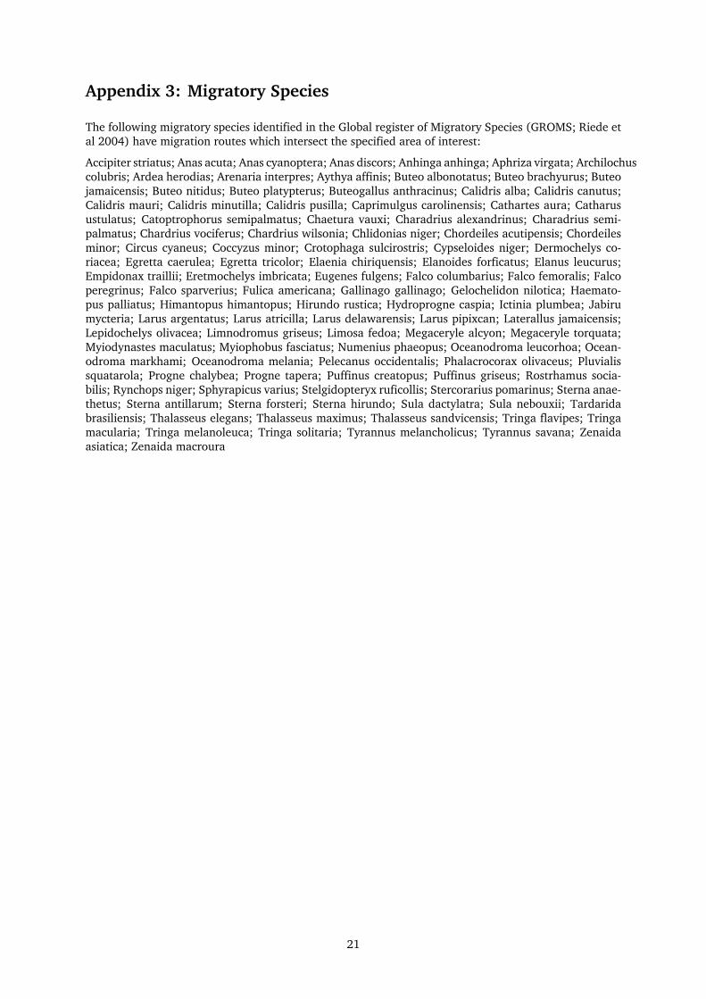
Appendix 3: Migratory Species

The following migratory species identified in the Global register of Migratory Species (GROMS; Riede etal 2004) have migration routes which intersect the specified area of interest:

Accipiter striatus; Anas acuta; Anas cyanoptera; Anas discors; Anhinga anhinga; Aphriza virgata; Archilochuscolubris; Ardea herodias; Arenaria interpres; Aythya affinis; Buteo albonotatus; Buteo brachyurus; Buteojamaicensis; Buteo nitidus; Buteo platypterus; Buteogallus anthracinus; Calidris alba; Calidris canutus;Calidris mauri; Calidris minutilla; Calidris pusilla; Caprimulgus carolinensis; Cathartes aura; Catharusustulatus; Catoptrophorus semipalmatus; Chaetura vauxi; Charadrius alexandrinus; Charadrius semi-palmatus; Chardrius vociferus; Chardrius wilsonia; Chlidonias niger; Chordeiles acutipensis; Chordeilesminor; Circus cyaneus; Coccyzus minor; Crotophaga sulcirostris; Cypseloides niger; Dermochelys co-riacea; Egretta caerulea; Egretta tricolor; Elaenia chiriquensis; Elanoides forficatus; Elanus leucurus;Empidonax traillii; Eretmochelys imbricata; Eugenes fulgens; Falco columbarius; Falco femoralis; Falcoperegrinus; Falco sparverius; Fulica americana; Gallinago gallinago; Gelochelidon nilotica; Haemato-pus palliatus; Himantopus himantopus; Hirundo rustica; Hydroprogne caspia; Ictinia plumbea; Jabirumycteria; Larus argentatus; Larus atricilla; Larus delawarensis; Larus pipixcan; Laterallus jamaicensis;Lepidochelys olivacea; Limnodromus griseus; Limosa fedoa; Megaceryle alcyon; Megaceryle torquata;Myiodynastes maculatus; Myiophobus fasciatus; Numenius phaeopus; Oceanodroma leucorhoa; Ocean-odroma markhami; Oceanodroma melania; Pelecanus occidentalis; Phalacrocorax olivaceus; Pluvialissquatarola; Progne chalybea; Progne tapera; Puffinus creatopus; Puffinus griseus; Rostrhamus socia-bilis; Rynchops niger; Sphyrapicus varius; Stelgidopteryx ruficollis; Stercorarius pomarinus; Sterna anae-thetus; Sterna antillarum; Sterna forsteri; Sterna hirundo; Sula dactylatra; Sula nebouxii; Tardaridabrasiliensis; Thalasseus elegans; Thalasseus maximus; Thalasseus sandvicensis; Tringa flavipes; Tringamacularia; Tringa melanoleuca; Tringa solitaria; Tyrannus melancholicus; Tyrannus savana; Zenaidaasiatica; Zenaida macroura

21

Appendix 4: Data Sources

Georeferenced species records obtained from the GBIF occurrence API (http://www.gbif.org/occurrence)are shared according to the GBIF Data Use Agreement, which includes the provision that users of any dataaccessed through or retrieved via the GBIF Portal will always give credit to the original data publishers.The following table lists the data sources for all occurrence records which have been used in this analysis.

Angelo State Natural History Collections (ASNHC)Australian National Herbarium (CANB)Avian Knowledge NetworkBiologiezentrum Linz OberoesterreichCalifornia Academy of SciencesCarnegie MuseumsCentre for Genetic Resources, The NetherlandsComisión nacional para el conocimiento y uso de la biodiversidadConservatoire et Jardin botaniques de la Ville de Genève - GCornell Lab of OrnithologyCornell University Museum of VertebratesCosta Rica Bird ObservatoriesCouncil of Heads of Australasian Herbaria (CHAH)European Molecular Biology Laboratory (EMBL)Facultad de Ciencias, UNAMFairchild Tropical Botanic GardenField MuseumFlorida Museum of Natural HistoryGBIF-SwedenHarvard University HerbariaHerbarium of the University of AarhusInstituto Agronômico (IAC)Instituto Nacional de Biodiversidad (INBio), Costa RicaInstituto Nacional de Pesquisas da Amazônia - INPAInstituto de Botânica, São PauloInstituto de Ciencias NaturalesInstituto de Investigación de Recursos Biológicos Alexander von HumboldtInstituto de Pesquisas Jardim Botanico do Rio de JaneiroJBGPJames R. Slater Museum of Natural HistoryLouisiana State University Museum of Natural ScienceLund Botanical Museum (LD)MNHN - Museum national d'Histoire naturelleMichigan State University MuseumMissouri Botanical GardenMuseo Nacional de Costa RicaMuseum für Naturkunde BerlinMuseum of Biological Diversity, The Ohio State UniversityMuseum of Comparative Zoology, Harvard UniversityMuseum of Southwestern BiologyMuseum of Texas Tech University (TTU)Museum of Vertebrate ZoologyMuséum d'histoire naturelle de la Ville de Genève - MHNGNational Herbarium of New South WalesNational Museum of Natural History, Smithsonian InstitutionNatural History MuseumNatural History Museum of Los Angeles CountyNatural History Museum, University of OsloNatural History Museum, Vienna - Herbarium WNaturalis Biodiversity Center

22

North Carolina State Museum of Natural SciencesOcean Biogeographic Information SystemPontificia Universidad JaverianaRLSReal Jardín Botánico (CSIC)Red Nacional de Observadores de Aves (RNOA)Redpath Museum, McGill UniversityRoyal Botanic Garden EdinburghRoyal Botanic Gardens, KewRoyal Ontario MuseumSam Noble Oklahoma Museum of Natural HistorySan Diego Natural History MuseumSenckenbergStaatliche Naturwissenschaftliche Sammlungen BayernsStaatliches Museum für Naturkunde StuttgartTexas A&M University Biodiversity Research and Teaching CollectionsThe New York Botanical GardenUNIBIO, IBUNAMUniversidad Nacional de ColombiaUniversidad de AntioquiaUniversidad del ValleUniversidade Estadual Paulista - Rio ClaroUniversidade Estadual de Campinas - Instituto de BiologiaUniversidade Estadual de Feira de SantanaUniversidade Federal da ParaíbaUniversidade Federal de Minas GeraisUniversidade Federal do ParanáUniversidade Federal do PiauíUniversidade de BrasíliaUniversity of Alabama Biodiversity and SystematicsUniversity of Alaska Museum of the NorthUniversity of Alberta MuseumsUniversity of Amsterdam / IBEDUniversity of Arizona HerbariumUniversity of British ColumbiaUniversity of Colorado Museum of Natural HistoryUniversity of ConnecticutUniversity of Gda�sk, Dept. of Plant Taxonomy and Nature ConservationUniversity of Graz, Institute of Plant SciencesUniversity of Kansas Biodiversity InstituteUniversity of LethbridgeUniversity of Michigan Museum of ZoologyUniversity of South Florida HerbariumUniversity of Texas at El PasoUniversity of Toronto MississaugaUniversity of Vienna, Institute for Botany - Herbarium WUUniversity of Washington Burke MuseumUniversity of Wyoming Museum of VertebratesWestern Foundation of Vertebrate ZoologyWildlife SightingsYale University Peabody MuseumiNaturalist.orgnaturgucker.de

23