www.elsevier.com/locate/visres

Vision Research 45 (2005) 2549–2563

Pupillary evaluation of retinal asymmetry: Developmentand initial testing of a technique

Yanjun Chen a, Harry J. Wyatt a,*, William H. Swanson b

a Department of Biological Sciences, SUNY State College of Optometry, 33 West 42nd Street, New York, NY 10036, USAb Department of Clinical Sciences, SUNY State College of Optometry, 33 West 42nd Street, New York, NY 10036, USA

Received 1 October 2004; received in revised form 2 March 2005

Abstract

Glaucomatous damage to upper and lower retina is often unequal. We have developed a rapid, objective, quantitative measure of

asymmetry of retinal sensitivity, using infrared pupillometry and pairs of large stimuli that are symmetric about the horizontal

meridian. Results for a group of 11 young subjects free of eye disease indicate that the distribution of asymmetry is close to a normal

distribution centered near upper/lower symmetry. Some subjects showed modest amounts of asymmetry, which was relatively uni-

form within each eye, and between the two eyes, of the subject. This approach to determination of asymmetry within an eye is poten-

tially applicable to testing patients with glaucoma. The narrowness of the distribution should make it possible to detect asymmetries

caused by disease.

� 2005 Elsevier Ltd. All rights reserved.

Keywords: Pupillary light reflex; RAPD; Retina; Human

1. Introduction

Static automated perimetry is generally regarded as

the ‘‘gold standard’’ for assessment of glaucomatous vi-sual field defects. However, like many subjective tests,

perimetry is demanding, performance is related to expe-

rience, and the results can be influenced by factors such

as anxiety, alertness and a patient�s desire to give nega-

tive results. Because conventional perimetry measures

the luminance increment threshold with a considerable

number of small stimuli, it is usually relatively slow (a

test may take from 5–7 min up to 10 min for one eye,depending on the test employed, Bengtsson & Heijl,

1998; Bengtsson, Heijl, & Olsson, 1998; Choplin & Ed-

wards, 1995). Perimetric results can show relatively large

test–retest variability, especially in damaged areas, and

0042-6989/$ - see front matter � 2005 Elsevier Ltd. All rights reserved.

doi:10.1016/j.visres.2005.04.003

* Corresponding author. Tel.: +1 212 780 5163; fax: +1 212 780 5174.

E-mail address: wyatt@sunyopt.edu (H.J. Wyatt).

differentiation between true progression of glaucoma

and random variation can require many tests (Chauhan

& Johnson, 1999; Flammer, Drance, & Zulauf, 1984;

Heijl, Lindgren, & Lindgren, 1989; Wall, Kutzko, &Chauhan, 1997).

Because of these factors, efforts have been made to

develop alternatives to visual fields that are objective,

easy to perform, rapid to administer, and reliable. For

example, one objective test which has been used recently

in the clinical evaluation of glaucoma is the visual

evoked potential (e.g., the multifocal VEP, Hood

et al., 2004). However, the small signal amplitude re-quires averaging over many repetitions to obtain distin-

guishable responses, prolonging the test. Another

approach to developing an objective functional test is

the use of the pupillary light reflex (PLR) to assess reti-

nal function. The PLR has been shown in many studies

to serve as an indicator of retinal status (Johnson, Hill,

& Bartholomew, 1988; Lagreze & Kardon, 1998; Loe-

wenfeld & Rosskothen, 1974; Lowenstein, Kawabata,

2550 Y. Chen et al. / Vision Research 45 (2005) 2549–2563

& Loewenfeld, 1964; Thompson, Montague, Cox, &

Corbett, 1982).

‘‘Pupil perimetry’’, a technique employing infrared

pupillometry, was developed more than a decade ago

as a way of evaluating visual fields objectively (Fankha-

user & Flammer, 1989; Hong, Narkiewicz, & Kardon,2001; Kardon, 1992; Kardon, Kirkali, & Thompson,

1991; Ukai, 1985; Wilhelm et al., 2000; Yoshitomi, Mat-

sui, Tanakadate, & Ishikawa, 1999). Most studies of

pupil perimetry employ a stimulus arrangement similar

to that of conventional perimetry. (Wilhelm�s techniqueemploys a stimulus similar to multifocal electroretino-

graphic (ERG) stimuli.) Instead of measuring thres-

holds, the PLR amplitude is measured, using a spotstimulus of fixed suprathreshold luminance, presented

at each test location. The subject�s task in pupil perime-

try—staring at a fixation point—is easy to perform; sub-

jects do not have to make judgments about stimulus

visibility. However, current pupil perimetric tests are

still quite lengthy (about 30–40 min), due to the nature

of the stimulus layout, and defects may not be well cor-

related with perimetry in cases of glaucoma (Kardon,1992). As with psychophysical perimetry, a substantial

amount of within- and between-subject variability has

been reported in results with pupil perimetry (Turtschi,

Bergamin, Dubler, Schotzau, & Zulauf, 1994).

The experimental design that we have developed is

somewhat similar to the design of the ‘‘swinging flash-

light test’’, which has long been a useful clinical test to

detect relative afferent pupillary defects (RAPD) be-tween the two eyes (Levatin, 1959). The swinging flash-

light test detects an RAPD as a significant asymmetry

between the two eyes. In our test, instead of making a

comparison between the two eyes, the relative pupillo-

motor sensitivity is determined for corresponding supe-

rior and inferior retinal territories within the same eye.

In human retina, the distribution of nerve fiber bun-

dles is relatively symmetric about the horizontal meri-dian (Vrabec, 1966). During the progress of glaucoma,

damage to nerve fibers is often asymmetric in upper

vs. lower retina (Aulhorn & Karmeyer, 1977; Hart &

Becker, 1982; Heijl & Lundqvist, 1984; Katz, Quigley,

& Sommer, 1995). Asymmetric functional changes char-

acteristic of glaucomatous retinal nerve fiber damage

may be detectable as asymmetries in relative sensitivity

of the PLR in the upper and lower hemifield. This issomewhat similar to the ‘‘glaucoma hemifield test’’

(GHT), which also tests for visual asymmetry between

upper and lower retina; however the GHT starts with

data from conventional perimetry, and processes those

data to determine patterns of asymmetry (Asman &

Heijl, 1992a, 1992b; Katz et al., 1995).

The present approach measures asymmetries of the

PLR using large stimuli, which may be thought of asusing the same retina as a control. An internal control

of this sort could potentially reduce test–retest variabil-

ity. This paper describes the new methodology and its

initial application to normal subjects.

2. Methods

2.1. Apparatus

The instrumentation consisted of a stimulus display

monitor (Radius PressView 21SR, Miro Displays, Inc.,

Germany) driven by a Power Macintosh G3 computer,

and a PC-based infrared pupillometer (ISCAN EC-

101, ISCAN, Inc., Burlington, MA).

The Macintosh computer controlled the stimulus dis-play. Software was developed using the Psychophysics

Toolbox (Brainard, 1997) with Yi–Zhong Wang�s inter-face in Matlab 5.2 (The MathWorks). This provides

high-level access to the C-language VideoToolbox (Pelli,

1997). Stimulus shape, fixation point, intensity of the

stimulus and background, and temporal frequency of

the stimulus were selected from a menu. Three digital

I/O lines connected the Macintosh and the PC. One lineturned pupillometer recording on and off. The other two

digital lines carried signals indicating timing of the stim-

ulus; these two lines were recorded together with the

pupil data.

The display monitor was a 2100 CRT monitor with

38.0 · 27.8 cm active area, resolution 832 · 624 pixels,

and frame rate 75 Hz. The monitor was 75 cm from

the recorded eye. The visual angle subtended at theeye was 29.1� horizontally and 21.8� vertically.

The infrared pupillometer was a PC-based dark-pupil

system, consisting of a resident card, a video camera and

monitor, and an infrared spotlight. The infrared light

source and video camera were placed at approximately

the same distance from the subject as the display moni-

tor, and appropriately aligned so that a pupil signal was

observed on the PC. The subject�s eye could also be ob-served by the experimenter on the video monitor. The

pupillometer recorded the horizontal diameter of the pu-

pil 60 times/s; data were saved in both software-specific

raw data files and ASCII files.

The luminance distribution of the display monitor was

calibrated using a luminance meter (LS-100, Minolta,

Japan). Calibrations were obtained for several locations

on the monitor, expressing luminance as a function ofDAC number output to the monitor. (All guns were dri-

ven equally.) OneDAC level was selected from themiddle

of the log-linear portions of these functions, and monitor

luminancewas then determined at a grid of 9 · 7 positions

for that particular nominal luminance. Each ‘‘stimulus’’

(see below) actually consisted of a pair of stimuli, one

above and one below the horizontal meridian. For a par-

ticular experimental stimulus pair, set at a uniform nom-inal luminance, an estimate of relative pupillomotor

Y. Chen et al. / Vision Research 45 (2005) 2549–2563 2551

effectiveness was obtained as follows: The standard curve

of luminance vs. DAC value was used to set one DAC

value used for the entire stimulus. The nominal luminance

thus produced was multiplied by a correction factor for

each grid point, determined from the grid measurements,

giving an estimate of actual luminance at each grid loca-tion. Since pupillomotor sensitivity is not uniform across

the retina, these numbers were multiplied by another set

of scale factors relating pupillomotor sensitivity at each

location to sensitivity at a central location (the ‘‘pupillary

hill of vision’’) (Bouma, 1965; Kardon et al., 1991; Kar-

don & Thompson, 1994). These numbers were summed

over the set of grid points inside each member of the par-

ticular stimulus pair, giving one final number for each ofthe members of the pair. The final two numbers, give an

estimate of the relative pupil sensitivity to the two stimuli

to be expected as a result of asymmetries in the apparatus,

as well as non-uniformity of pupillomotor sensitivity. The

values found by this procedure gave very small estimates

of differences in sensitivity (0.001–0.005 log units), and

inhomogeneities of screen luminance were not considered

further.

Fig. 1. (a) Frequency distribution of focal retinal regions of glaucomatous da

the outlines of the three stimulus pairs used in the present study: paracentr

instances of loss in an area. (b) Stimulus layout on the display monitor. All

The dots represent the test grid for threshold perimetry (6� offset grid); dot

2.2. Stimuli

During the progress of glaucoma, focal damage of

retinal ganglion cells often affects vision in paracentral,

Bjerrum, and peripheral nasal regions of the visual field

(Fig. 1(a)). The form of the most likely regions for smallvisual field defects, and also the boundaries of larger

defects, tend to reflect, approximately, the retinal nerve

fiber bundle layout (Aulhorn & Karmeyer, 1977; Hart &

Becker, 1982; Heijl & Lundqvist, 1984; Weber & Ulrich,

1987, 1991). This provided the basis for the stimulus

design used in the present study. Three stimuli—para-

central, ‘‘Bjerrum’’, and peripheral—were designed to

cover much of the central visual field, an area 30� wide(20� nasal to 10� temporal) · 20� high (Fig. 1(b)). For

paracentral and Bjerrum stimuli, the fixation point was

in the center of the screen; for the peripheral stimulus,

the fixation point was moved 6� temporally, so that

the peripheral stimulus extended out to 20� eccentricityin the nasal field.

Achromatic stimuli were used to elicit pupil re-

sponses. Each stimulus consisted of two parts, located

mage (adapted from Aulhorn & Karmeyer, 1977). Gray/white lines are

al, Bjerrum, and peripheral. Key to shading scale indicates percent of

stimuli are for a right eye; the fixation point is indicated by an ‘‘X’’.

size is Goldman size III stimulus size to scale.

2552 Y. Chen et al. / Vision Research 45 (2005) 2549–2563

in upper and lower visual field, that were mirror images

about the horizontal meridian (Fig. 1(b)). For each

experimental trial, the two parts of the stimulus were

turned on and off alternately in the upper and lower vi-

sual field. The luminance of the lower portion of a stim-

ulus pair was fixed at 40 cd/m2, and the luminance of theupper portion cycled over three luminance levels: 24, 34,

and 48 cd/m2. (The middle luminance of the upper por-

tion was less than the fixed luminance of the lower por-

tion because, in preliminary experiments with three

subjects, we found indications that the pupillomotor

sensitivity of superior retina was less than that of infe-

rior retina.) The luminance of each stimulus was

0.01 cd/m2 when it was turned off. Outside of the stimu-lus boundaries was a uniform background (5 cd/m2).

During stimulus presentation, first, the upper part was

turned on for 1 s while the lower part was turned off;

then the lower part was turned on for 1 s while the upper

part was turned off, and so on. (The sequence is shown

schematically in Fig. 3(a)) At each transition, the pupil

constricted. A complete stimulus cycle lasted 6 s, and

the stimulus cycle was repeated three times per trial, soone trial lasted 18 s.

Each subject was tested in two sessions, separated by

1–3 weeks, to assess between-session variability. During

each session, a complete set of six trials was performed

(three stimuli for each eye); after a break of approxi-

mately 30 min, the six conditions were repeated in a

different sequence to assess within-session variability.

The stimulus sequence, and the order of eye tested,were counterbalanced to minimize any effect of sequence

(e.g., fatigue or practice effects). One stimulus sequence

consisted of three trials presented to one eye, using each

of the three stimuli. (There were six possible sequences.)

Across all subjects, each sequence was used 13–16 times.

If the first test of a particular subject began with the left

eye, the second test in that session would begin with the

right eye; in the second session for that subject, the se-quence would be reversed. The first eye tested for each

subject in their first session was alternated between the

two eyes from one subject to the next.

2.3. Subjects

There were 11 subjects (6 males and 5 females), aged

25–40 years old (29.7 ± 5.2). The subjects were recruitedfrom the community at SUNY State College of Opto-

metry. All subjects had passed a general ocular examina-

tion at the University Optometric Center. Inclusion

criteria were: best corrected visual acuity 20/25 or better,

intraocular pressure less than 21 mmHg, normal slit-

lamp and direct ophthalmoscopy exams, spherical

refractive error less than ±5.0D and cylindrical refrac-

tive error less than ±3.0D. Exclusion criteria were: a pri-mary relative with glaucoma, or medication that would

have an effect on pupil function. The study was ap-

proved by the SUNY College of Optometry Institu-

tional Review Board (IRB), and written informed

consent was obtained from each subject after the nature

of the experiment was explained in detail.

2.4. Protocol

Subjects sat in an examination chair with a head rest,

adjusted to align the subject with the stimulus display

and the eyetracker system. The eye not being tested

was covered with an opaque eye patch. After the pupil-

lometer signal was stable, a stimulus was presented on

the display monitor, with a red cross as a fixation point.

The subject was asked to fixate the red cross, and theexperimenter checked for a pupil signal. Usually, the

pupil gave a large response at the onset of the stimulus,

and after several cycles reached steady oscillatory

behavior. After such responses were observed on the

PC, the experimenter alerted the subject, and then began

recording. Pupil diameter and a digital signal of the

stimulus timing were recorded for the 18 s duration of

a trial (see Stimuli). After data were obtained fromone eye for the three stimuli, the subject was instructed

to switch the eyepatch, and the other eye was studied. A

complete set of tests (all three stimuli for both eyes) typ-

ically took approximately 5 min.

Blinking reduces the amount of light entering the eye

and contaminates the pupil record. Subjects were asked

to make a moderate effort not to blink during the

recording periods, and were told that it was fine to blinkall they wanted at other times. If a subject blinked more

than three times within one trial, the data were dis-

carded and the same condition was repeated.

2.5. Analysis of pupil records

A software program was developed to analyze the pu-

pil responses using Igor Pro 4.0 (WaveMetrics, Inc.,Lake Oswego, OR). The data analyzed consisted of hor-

izontal pupil diameter and timing signals of the stimulus

(see above).

Initial processing of pupil data consisted of blink

detection and removal, followed by digital filtering of

the pupil diameter signal. Blinks were detected by differ-

entiating the pupil diameter signal (2-point difference)

and using a rate-of-change threshold. The end of a blinkwas located with an algorithm using pupil diameter and

rate-of-change. Once demarcated, each blink was re-

placed with a linear data segment connecting the values

before and after the blink. Filtering employed the bino-

mial smoothing algorithm in Igor Pro, with a corner

frequency at approximately 5 Hz.

2.5.1. Determination of pupil response amplitudes

Under the luminance conditions of the present study,

if one of the stimuli was turned on and remained on at a

Fig. 2. Testing the exponential fit used to estimate ‘‘baseline’’. (a)

Example of curve fitting for one stimulus presentation (pupil data are

from average of three repeat cycles). Stimulus was modified so that

each stimulus presentation lasted 2 s, instead of 1 s. Thick solid line is

the fitted curve. Thick dotted line is the extrapolation of the fitted

curve. Arrows indicate stimulus onset. The fit is made to a sample of

pupil data from 800 to 1200 ms after stimulus onset. (1 s is the time of

the next stimulus onset for the standard stimulus used in the present

experiments.) The difference between the fitted and extrapolated curve

and the pupil record was determined at each time interval (60/s). (b)

Mean ± SD of the difference (fitted–actual) between fitted curve and

actual pupil record. The data were taken from exponential fitting to the

averaged pupil constriction for one trial using each of the three stimuli

(paracentral, Bjerrum and peripheral stimuli; subject YN1). For the

averaged data from each trial, fitting was carried out at each of the six

stimulus onsets. (Each mean and SD is based on 3 · 6 = 18 samples.)

Y. Chen et al. / Vision Research 45 (2005) 2549–2563 2553

constant luminance, the pupil would typically begin to

constrict 200–400 ms after stimulus onset, and reach

peak constriction at 600–800 ms after stimulus onset.

After that, the pupil would gradually redilate and reach

a steady state at about 1200 ms. In this simple situation,

the amplitude of the pupil response is the difference inpupil diameter between peak constriction and the pre-

stimulus level. However, if a second stimulus is pre-

sented before the pupil reaches steady state, the second

response begins before the first has reached a steady

level. This makes determination of the appropriate base-

line level for the second stimulus response difficult. This

was generally the case for the stimuli used in the present

experiments.To deal with problem noted above, we developed a

way of determining a baseline level: a portion of the

pupil curve was considered—from the peak of pupil

constriction to a point about 400 ms later, amounting

to a window from about 800 to 1200 ms after stimulus

onset. This portion of the redilation was fitted with a

decaying exponential function, and the fitted exponen-

tial was extrapolated to the time of the next peak of pu-pil constriction. The difference between the next peak

and the fitted curve was used as the amplitude of the

next pupil constriction (Figs. 2 and 3(b)). (It is impor-

tant to note that 400 ms after one peak—the end of

the data window used for the extrapolation—precedes

the beginning of the next pupil response.)

In order to test the accuracy of the fitting process, we

modified the stimulus so that each part of the stimulusappeared for 2 s instead of 1 s (Fig. 2). In this case, there

was enough time for the pupil to reach a steady level be-

fore the next constriction began. As with the standard

stimulus timing, a 400 ms sample from the interval

800–1200 ms after an onset of upper or lower stimulus

was used to perform an extrapolation. It was now pos-

sible to compare the extrapolation to the pupil record

at times near 1600 ms after stimulus onset. (With thestandard stimulus timing, this is the approximate time

of the peak constriction to the next stimulus onset.)

Fig. 2 shows the mean and SD (18 trials) of the differ-

ence between the fitted and the actual data at each sam-

ple time, for subject YN1. The mean differences are close

to zero, indicating that there was little tendency for the

fitted curve to be larger or smaller than the actual data.

The mean magnitude of the difference between fittedcurve and actual data, across all stimuli, was 0.04 mm.

To evaluate the significance of this, a segment of the pu-

pil record 1500–2000 ms after stimulus onset was used to

estimate the noise. (The pupil reached steady state about

1200 ms after stimulus onset.) The SD of pupil diameter

for this segment of the data was 0.04 mm. Thus, the

error in estimating the baseline was comparable to the

noise level in the pupil measurements. This procedurefor validating the baseline extrapolation was repeated

in another subject with similar results.

2.6. Determination of ‘‘response balance’’

For the three luminance pairs in one stimulus trial:

each stimulus presentation (S) gave a pupil constriction

(R). This allowed determination of a ‘‘response balance’’

value for each pair of stimuli (Fig. 3), where

Response balancei ¼ ðRUi � RLiÞ=ðRUi þ RLiÞ ð1Þ

Li ði ¼ 1; 2; 3Þ: ith stimulus presented in the lower

visual field;RLi ði ¼ 1; 2; 3Þ: pupil constriction resulting from Li;

Ui ði ¼ 1; 2; 3Þ: ith stimulus presented in the upper

visual field;

RUi ði ¼ 1; 2; 3Þ: pupil constriction resulting from Ui.

One trial consisted of three upper/lower stimulus

values, giving three response balance values.

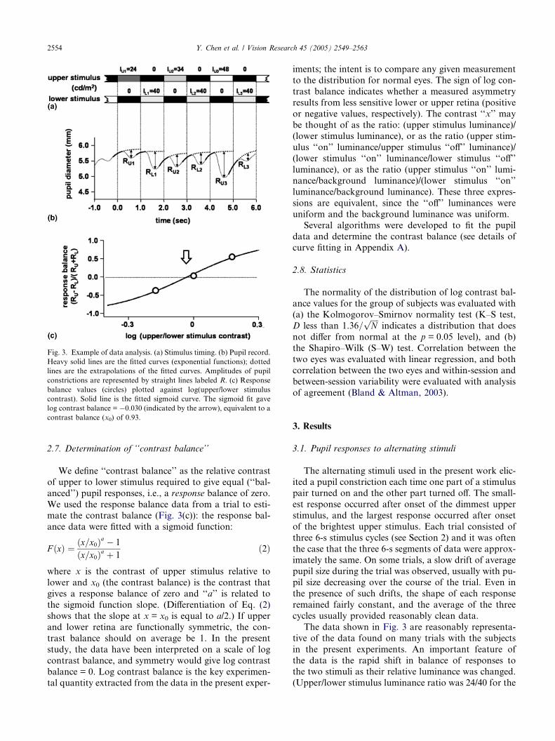
Fig. 3. Example of data analysis. (a) Stimulus timing. (b) Pupil record.

Heavy solid lines are the fitted curves (exponential functions); dotted

lines are the extrapolations of the fitted curves. Amplitudes of pupil

constrictions are represented by straight lines labeled R. (c) Response

balance values (circles) plotted against log(upper/lower stimulus

contrast). Solid line is the fitted sigmoid curve. The sigmoid fit gave

log contrast balance = �0.030 (indicated by the arrow), equivalent to a

contrast balance (x0) of 0.93.

2554 Y. Chen et al. / Vision Research 45 (2005) 2549–2563

2.7. Determination of ‘‘contrast balance’’

We define ‘‘contrast balance’’ as the relative contrast

of upper to lower stimulus required to give equal (‘‘bal-

anced’’) pupil responses, i.e., a response balance of zero.

We used the response balance data from a trial to esti-mate the contrast balance (Fig. 3(c)): the response bal-

ance data were fitted with a sigmoid function:

F ðxÞ ¼ ðx=x0Þa � 1

ðx=x0Þa þ 1ð2Þ

where x is the contrast of upper stimulus relative to

lower and x0 (the contrast balance) is the contrast thatgives a response balance of zero and ‘‘a’’ is related to

the sigmoid function slope. (Differentiation of Eq. (2)

shows that the slope at x = x0 is equal to a/2.) If upper

and lower retina are functionally symmetric, the con-

trast balance should on average be 1. In the present

study, the data have been interpreted on a scale of log

contrast balance, and symmetry would give log contrast

balance = 0. Log contrast balance is the key experimen-tal quantity extracted from the data in the present exper-

iments; the intent is to compare any given measurement

to the distribution for normal eyes. The sign of log con-

trast balance indicates whether a measured asymmetry

results from less sensitive lower or upper retina (positive

or negative values, respectively). The contrast ‘‘x’’ may

be thought of as the ratio: (upper stimulus luminance)/(lower stimulus luminance), or as the ratio (upper stim-

ulus ‘‘on’’ luminance/upper stimulus ‘‘off’’ luminance)/

(lower stimulus ‘‘on’’ luminance/lower stimulus ‘‘off’’

luminance), or as the ratio (upper stimulus ‘‘on’’ lumi-

nance/background luminance)/(lower stimulus ‘‘on’’

luminance/background luminance). These three expres-

sions are equivalent, since the ‘‘off’’ luminances were

uniform and the background luminance was uniform.Several algorithms were developed to fit the pupil

data and determine the contrast balance (see details of

curve fitting in Appendix A).

2.8. Statistics

The normality of the distribution of log contrast bal-

ance values for the group of subjects was evaluated with(a) the Kolmogorov–Smirnov normality test (K–S test,

D less than 1.36=ffiffiffiffiN

pindicates a distribution that does

not differ from normal at the p = 0.05 level), and (b)

the Shapiro–Wilk (S–W) test. Correlation between the

two eyes was evaluated with linear regression, and both

correlation between the two eyes and within-session and

between-session variability were evaluated with analysis

of agreement (Bland & Altman, 2003).

3. Results

3.1. Pupil responses to alternating stimuli

The alternating stimuli used in the present work elic-

ited a pupil constriction each time one part of a stimuluspair turned on and the other part turned off. The small-

est response occurred after onset of the dimmest upper

stimulus, and the largest response occurred after onset

of the brightest upper stimulus. Each trial consisted of

three 6-s stimulus cycles (see Section 2) and it was often

the case that the three 6-s segments of data were approx-

imately the same. On some trials, a slow drift of average

pupil size during the trial was observed, usually with pu-pil size decreasing over the course of the trial. Even in

the presence of such drifts, the shape of each response

remained fairly constant, and the average of the three

cycles usually provided reasonably clean data.

The data shown in Fig. 3 are reasonably representa-

tive of the data found on many trials with the subjects

in the present experiments. An important feature of

the data is the rapid shift in balance of responses tothe two stimuli as their relative luminance was changed.

(Upper/lower stimulus luminance ratio was 24/40 for the

Y. Chen et al. / Vision Research 45 (2005) 2549–2563 2555

leftmost response pair, and 48/40 for the rightmost re-

sponse pair.)

3.2. Distribution of ‘‘contrast balance’’ values

Fig. 4(a) shows the contrast balance data(mean ± SD) grouped by subject (all 24 trials from each

subject grouped together). Individual average values of

contrast balance for the 11 subjects ranged from �0.15

to +0.23 log units. At the bottom of Fig. 4(a) are the

data for the entire subject group (all individual trial re-

sults pooled). The smooth curve with the histogram is

the best-fit normal distribution, which has cen-

ter = 0.019 and SD = 0.162. The frequency distributionwas normal according to a Kolmogorov–Smirnov test

(d = 0.034, p > 0.2); a Shapiro–Wilk test suggested a

slight deviation of the center towards the positive side,

probably resulting from a group of points at the positive

end of the distribution, visible in the histogram. It is

apparent that the data for each subject generally form

a somewhat narrower distribution than the data for all

subjects pooled. (For 9 out of 11 subjects, the SD foreach subject was smaller than that for the whole subject

group; the other 2 subjects had SD�s equal to, or slightlylarger than, the group SD.) The broader curve for the

entire subject group is clearly the result of different

Fig. 4. Contrast balance distributions for the subject group. (a)

Contrast balance distributions for all individual trials from each

subject, grouped by subject (mean ± SD). There were generally 24

trials for each subject, so most SEM error bars would not be larger

than the symbol size. The distribution and mean ± SD shown at the

bottom are for pooled data from all subjects. The smooth curve is the

best-fit normal distribution for the pooled data: the data are not

significantly different from a normal distribution according to a K–S

test (d = 0.07, p > 0.05). With a S–W test, the distribution deviates

from normal (W = 0.97, p < 0.05), due to the small cluster of points at

the positive end of the distribution. (b) Comparison of the two eyes in

each subject. The mean ± SD for each stimulus in each subject�s righteye is plotted against the mean ± SD for the left eye. Filled circles:

paracentral stimulus; open circles: Bjerrum stimulus; inverted triangles:

peripheral stimulus.

subjects having different mean values. (The SEM values

for Fig. 4(a) were typically no larger than the symbol

size; thus, subjects with means near one end of the group

differed significantly in their mean values from subjects

with means near the other end.)

In a related finding, linear regression analysis showedthat the average contrast balance for a subject�s right eyewas correlated with (and nearly equal to) that for the left

eye (r = 0.82, r2 = 0.67) (Fig. 4(b)). Analysis of agree-

ment (not shown) found no significant difference be-

tween eyes: the distribution of differences between the

two eyes was Gaussian (K–S: D = 0.13, p > 0.05) and

centered at 0.007 log units with SD = 0.085 log units

(95% CI = �0.160 to 0.174 log units). When the datafor the different stimuli were separated, the correlation

was somewhat poorer for the paracentral stimulus (filled

circles; r = 0.74) than for the Bjerrum stimulus (open cir-

cles; r = 0.89) and the peripheral stimulus (inverted tri-

angles; r = 0.91).

Grouping results for each of the three stimuli across

subjects, it was found that there were no significant dif-

ferences in the contrast balance among stimuli (1-wayANOVA, F = 0.4, p = 0.7); the average log contrast bal-

ance was approximately zero for each stimulus. (Vari-

ances for the three stimuli ranged from 0.02 to 0.03,

so our sample size was adequate to detect a 0.2 log unit

difference between two stimuli with a power of 0.80 at

confidence level p < 0.05.)

3.3. Within-session and between-session variability

Within-session variation was taken to be the differ-

ence between log contrast balance values found for

two repeat test trials performed during the same session

(test 1 minus test 2) (Fig. 5, top). Data from the first ses-

sion were used for the analysis of within-session vari-

ability; if data were not available from the first session

for a particular stimulus condition, data from the sec-ond session were used. Within-session variation was dis-

tributed approximately normally (K–S: D = 0.12, p >

0.05; SW: W = 0.94, p = 0.001). Fig. 5(top left) shows

the difference between log contrast balance values plot-

ted against the average of the two (Bland & Altman,

2003). The center of the distribution of within-session

variation was approximately zero, and the 95% confi-

dence interval was �0.30 to +0.28 log units (Fig. 5,top). Since it is also useful to have an estimate of the size

of the variation, independent of sign, we also calculated

the amount of within-session variation (absolute value of

difference between log contrast balance values for the

two tests); the average value of this for each of the three

stimuli varied between 0.07 and 0.14 log units, with a

mean of about 0.10 log units.

Between-session variation was taken to be the differ-ence between the log contrast balance values for the two

sessions (session 1 minus session 2). For each session

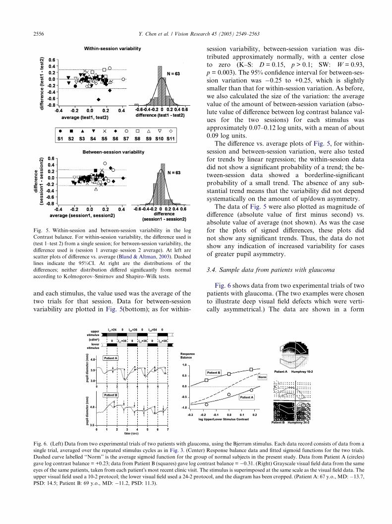
Fig. 5. Within-session and between-session variability in the log

Contrast balance. For within-session variability, the difference used is

(test 1–test 2) from a single session; for between-session variability, the

difference used is (session 1 average–session 2 average). At left are

scatter plots of difference vs. average (Bland & Altman, 2003). Dashed

lines indicate the 95%CI. At right are the distributions of the

differences; neither distribution differed significantly from normal

according to Kolmogorov–Smirnov and Shapiro–Wilk tests.

2556 Y. Chen et al. / Vision Research 45 (2005) 2549–2563

and each stimulus, the value used was the average of the

two trials for that session. Data for between-session

variability are plotted in Fig. 5(bottom); as for within-

Fig. 6. (Left) Data from two experimental trials of two patients with glaucom

single trial, averaged over the repeated stimulus cycles as in Fig. 3. (Center)

Dashed curve labelled ‘‘Norm’’ is the average sigmoid function for the group

gave log contrast balance = +0.23; data from Patient B (squares) gave log con

eyes of the same patients, taken from each patient�s most recent clinic visit. Th

upper visual field used a 10-2 protocol; the lower visual field used a 24-2 proto

PSD: 14.5; Patient B: 69 y.o., MD: �11.2, PSD: 11.3).

session variability, between-session variation was dis-

tributed approximately normally, with a center close

to zero (K–S: D = 0.15, p > 0.1; SW: W = 0.93,

p = 0.003). The 95% confidence interval for between-ses-

sion variation was �0.25 to +0.25, which is slightly

smaller than that for within-session variation. As before,we also calculated the size of the variation: the average

value of the amount of between-session variation (abso-

lute value of difference between log contrast balance val-

ues for the two sessions) for each stimulus was

approximately 0.07–0.12 log units, with a mean of about

0.09 log units.

The difference vs. average plots of Fig. 5, for within-

session and between-session variation, were also testedfor trends by linear regression; the within-session data

did not show a significant probability of a trend; the be-

tween-session data showed a borderline-significant

probability of a small trend. The absence of any sub-

stantial trend means that the variability did not depend

systematically on the amount of up/down asymmetry.

The data of Fig. 5 were also plotted as magnitude of

difference (absolute value of first minus second) vs.absolute value of average (not shown). As was the case

for the plots of signed differences, these plots did

not show any significant trends. Thus, the data do not

show any indication of increased variability for cases

of greater pupil asymmetry.

3.4. Sample data from patients with glaucoma

Fig. 6 shows data from two experimental trials of two

patients with glaucoma. (The two examples were chosen

to illustrate deep visual field defects which were verti-

cally asymmetrical.) The data are shown in a form

a, using the Bjerrum stimulus. Each data record consists of data from a

Response balance data and fitted sigmoid functions for the two trials.

of normal subjects in the present study. Data from Patient A (circles)

trast balance = �0.31. (Right) Grayscale visual field data from the same

e stimulus is superimposed at the same scale as the visual field data. The

col, and the diagram has been cropped. (Patient A: 67 y.o., MD: �13.7,

Y. Chen et al. / Vision Research 45 (2005) 2549–2563 2557

analogous to the pupil records of Fig. 3. Along with the

pupil data are shown the visual fields of the tested eyes,

with the outline of the pupil stimulus superimposed. A

comparison of the visual field data with the pupil data

shows that the areas of retina with the visual field defects

produced pupillomotor signals that were much weakerthan the signals from the areas of retina giving relatively

normal visual field results.

4. Discussion

In the present study, we have developed a method for

determining the amount of functional asymmetry be-tween regions of upper and lower retina, using the pupil-

lary light reflex. In the present form, the test typically

took about 5 min for all three stimuli in both eyes.

The data suggest functional near-symmetry between

superior and inferior retina in normal eyes, with the

population mean very near to symmetry but some indi-

viduals having asymmetries which were mild in extent

but consistent in both eyes and for all stimuli.

4.1. Design of the stimulus

In the present experiments, large stimuli were used

because they offer the possibility of rapid testing. The

PLR has the property of almost unlimited spatial sum-

mation (Schweitzer & Bouman, 1957): when a stimulus

covers a large retinal area, the entire area contributesto the pupil response. The intent of these studies is to ap-

ply the techniques to patients with glaucoma; however,

one potential problem is that, with a large stimulus,

the pupil response will only show a significantly reduced

response if a substantial fraction of the participating

ganglion cells covered by the stimulus are damaged.

We selected stimuli which should be sensitive to the

kinds of asymmetry which are often present in earlystages of glaucoma.

The short duration of the present test also depends in

part on the use of suprathreshold stimuli. Working at

suprathreshold levels may avoid problems commonly

encountered with threshold measurements, such as low

values of signal/noise, different definitions of threshold

in different studies, and the time required to estimate

the threshold using psychophysical algorithms.In determining the experimental responses (see Sec-

tion 2), we treated the stimulus presentation as a

sequence of three upper/lower stimulus pairs. Although

the pairing might seem arbitrary, it is important to note

that in the stimulus sequence U1/L1/U2/L2/U3/L3 (where

L1 = L2 = L3), in the stimulus pair U1/L1, each stimulus

follows the other stimulus in the pair. (U1 follows L3

which is identical to L1). The same type of symmetryholds for pairs U2/L2 and U3/L3. This symmetry is an

important feature of the stimulus presentation. (There

is an assumption made that still-earlier stimuli do not

significantly affect the results; e.g., that the U2 stimulus

that precedes the L2 that precedes the U3 does not affect

the response to U3.)

4.2. Light scatter

Since the pupillary light reflex integrates light over

large areas of visual space, it is important to consider

to what extent light scatter could have contaminated

or altered our results. We were particularly concerned

about this issue, which was our motive for having a

bright background—our brightest stimulus was only

one log unit brighter than our background luminance.This is a very conservative choice of background; in

pupil perimetry studies, the stimulus luminance has gen-

erally been at least two log units brighter than the back-

ground (Kardon, 1992; Kardon et al., 1991; Yoshitomi

et al., 1999).

Another aspect of the present experiments that re-

duces likelihood of light scatter effects involves the mode

of stimulus presentation. In an experimental trial using aBjerrum stimulus pair for example, the background pro-

vides considerable ‘‘defense’’ against effects of light scat-

ter into paracentral and peripheral areas. Light from the

upper Bjerrum stimulus does scatter into the territory of

the lower stimulus, but the amount of light is much less

than when the lower stimulus is turned on. Thus, the

simultaneous offset of the lower stimulus and onset of

the upper stimulus results in a drastic lessening illumina-tion of the retinal area of the lower stimulus. (In con-

trast, if the lower stimulus were off for some time, and

then the upper stimulus turned on, there would be

an increment in illumination within the territory of the

lower stimulus due to light scatter.) Further evidence

against a large role of light scatter in the present experi-

ments may be seen in Fig. 6: areas of retina which (from

the evidence of perimetry) were badly damaged, gavesubstantially less signal to the light reflex. The agree-

ment between visual loss and pupillomotor loss shown

in Fig. 6 argues against any very large ‘‘smearing’’ effect

due to light scatter.

A final factor that works to reduce light scatter effects

is the large stimulus size used in the present experiments;

if light scatter can be considered to occur primarily with-

in some angle hscatter of a ray�s direction, then extent ofspread expressed as a fraction of stimulus size will be

greater for a small stimulus than a large stimulus.

4.3. The use of extrapolation to determine

baseline levels for pupil responses

One aspect of our data analysis which deserves fur-

ther comment is the use of extrapolation to determinethe baseline value for each response (see Section 2 and

Figs. 2 and 3). We introduced this technique to cope

2558 Y. Chen et al. / Vision Research 45 (2005) 2549–2563

with situations in which small responses follow larger

ones. In such cases, the smaller response may appear

as an inflection (see Fig. 3, response RL3 ). If such a re-

sponse is measured as the difference between the pupil

diameter just prior to the beginning of the response

and the peak of the response, the measured amplitudemay be small or even zero, in spite of the fact that exam-

ination of the record shows that a response has clearly

occurred. As discussed in detail in Section 2, we esti-

mated baseline levels for each response by fitting curves

to portions of the pupil record. This approach gave rea-

sonable values for the effective amplitudes of small re-

sponses, while making little difference in the measured

amplitudes of larger responses. This is particularlyimportant in situations of unbalanced pupillomotor sen-

sitivity expected in many cases of glaucoma, where one

member of a stimulus pair, falling on damaged retina,

is likely to give a relatively weak response (Fig. 6). In

such a case, measuring response amplitudes without

using extrapolated baselines would underestimate the

amplitude of the response from damaged retina, and this

would have two major disadvantages: (i) By underesti-mating responses from the more damaged retina, the

estimate of contrast balance would be shifted in the

direction corresponding to greater damage, so that dam-

age will be overestimated. (ii) Overestimating the dam-

age would complicate the important task of developing

a meaningful scale for describing the extent of damage.

We also assessed the value of the extrapolation tech-

nique in some control experiments: using several normalsubjects, we ran trials using stimulus values which were

either (upper = 24, 36, 54/lower = 24), or (upper = 24/

lower = 24, 36, 54). These choices gave response se-

quences which closely resembled response sequences ob-

tained with symmetric stimuli in the presence of

moderate lower or upper visual field defects (moderately

damaged upper or lower retina), respectively. However,

unlike situations of actual retinal damage, the contrastbalance values determined for these two types of trials

are estimates of the relative sensitivity of the same two

areas of retina; therefore, if the stimulus luminances

are taken into account, they should give the same result.

We compared the results obtained by using amplitude

measurements with and without extrapolated baselines.

On average, the use of extrapolation was found to pro-

duce less spread in the estimations of contrast balance.It might be thought, from the considerations relating

to Fig. 2, that the need for baseline extrapolation could

be avoided by using 2-s instead of 1-s stimulus presenta-

tions. This was not done for two reasons: (a) With 2-s

presentations, trials would have lasted 36 s instead of

18 s, an unreasonably long time during which to request

minimal blinking. (b) The effectiveness of the test at

comparing afferent signals may on partial cancellationof the offset of one stimulus by the onset of the next

(see Section 4.5 below).

4.4. The distribution of ‘‘contrast balance’’ for normal

younger subjects

The approximately normal distribution of values of

the log contrast balance (Fig. 4) provides the potential

for detecting deviation of contrast balance from meannormal. Although the present study indicates that differ-

ent subjects can have different values of average contrast

balance, there tended to be less variation for a single

subject in regard to differences between the two eyes,

across the different stimuli, and across sessions. There-

fore, in addition to assessment of deviation from mean

normal by comparing a contrast balance value to the

distribution for the normal population, this intra-subjecthomogeneity may make further assessments possible,

e.g., by comparing differences between eyes and between

stimuli for a single eye.

The center of the distribution of log contrast balance

values was slightly positive (Fig. 4(a), bottom), which

suggests that, for pupil constriction, superior retina

(stimulated by the inferior stimulus in the pair) is slightly

more sensitive than inferior retina for the population.However, for some subjects the average log contrast bal-

ance was approximately zero, while for others it was dis-

placed positively or negatively from zero (Fig. 4(a)).

Differences in pupillomotor sensitivity between superior

and inferior retina have been observed in other studies,

though the results have not been uniform. In the present

results, the average balance was very close to symmetry.

Some other work, with 11 and 9 subjects, respectively,found average response amplitudes were 14% and 7%

greater for inferior retinal stimuli (superior visual field)

(Wilhelm et al., 2000; Yoshitomi et al., 1999). Our find-

ing that subjects can have mild idiosyncratic amounts of

imbalance may potentially explain the variability of

findings: if the degree of imbalance is normally distrib-

uted between subjects, as suggested by Fig. 4(a), results

from small samples could easily vary.A number of studies of visual function have indi-

cated greater sensitivity of superior retina, for absolute

threshold sensitivity (Krill, Smith, Blough, & Pass,

1968), contrast sensitivity (Skrandies, 1987), short-

wavelength automated perimetry (SWAP) (Sample,

Irak, Martinez, & Yamagishi, 1997), pattern electroret-

inography (ERG) and critical flicker fusion frequency

(CFF) (Skrandies, 1987). Standard perimetry has alsoindicated greater sensitivity of superior retina (Fig. 5

of Heijl, Lindgren, & Olsson, 1987). The differences in

sensitivity varied from about 0.04 log units to as much

as 0.4 log units—amounts which should be apparent

with our technique. Since results with the pupillary light

reflex indicate near-balance or favor superior retina

only slightly (see above), the visual asymmetry favoring

superior retina does not appear to be present inthe pupillomotor system as assessed from our small

sample.

Y. Chen et al. / Vision Research 45 (2005) 2549–2563 2559

Although much is known about the anatomical sub-

strate for the pupillary light reflex, there are still areas

of uncertainty. Histological studies of macaque monkey

indicate that approximately 10% of retinal ganglion cells

have axons projecting to the superior colliculus and pre-

tectum (Perry & Cowey, 1984; Rodieck, 1998), and thatneurons in the pretectum mediate the PLR (Clarke,

Zhang, & Gamlin, 2003a, 2003b; Gamlin, Zhang, &

Clarke, 1995; Hultborn, Mori, & Tsukahara, 1978; Tre-

jo & Cicerone, 1984). Recent studies have shown that a

small subset of retinal ganglion cells is intrinsically pho-

tosensitive and participates in the pupillary light reflex

pathway (Lucas et al., 2003). There is no evidence as

yet as to whether the ganglion cells responsible forpupillomotor signals have a different retinal distribution

from those responsible for visual signals, or whether the

paths of their axons to the optic nerve are the same. (It

has been suggested, for example, that the paths of retinal

M-cell axons might differ somewhat from the axons of

other ganglion cells in their path to the lamina cribrosa

(Wyatt, 1992).) To the extent that uncertainties remain

concerning the degree of similarity of the early afferentpathways for vision and for the pupillary light reflex,

anatomical differences may exist which could explain

the observed functional differences.

In the present experiments, the fixed luminance of the

lower stimulus was higher than the middle luminance

level of the upper stimulus. This was based on prelimin-

ary results, noted in Section 2, suggesting stronger pupil

responses from inferior vs. superior retina; thus, it wasanticipated that the distribution of log contrast balance

values would be centered at a negative value. Given the

finding that the distribution actually centered near zero,

a symmetric range of stimulus contrast may be prefera-

ble for future studies. However, given the method of

determining contrast balances, modest shifts of the set

of stimulus contrasts are not likely to change the distri-

bution of contrast balances found.

4.5. Within- and between-session variability

Within-session variability was defined as the variabil-

ity of a measurement repeated within a short time inter-

val. The present study found the mean magnitude of

within-session variability to be 0.10 log units.

Between-session variability is the variability of themeasurement between two sessions. The assessment of

between-session variability is important for determining

whether changes in test results are typical fluctuations or

reflect actual pathologic change. The present study

found the mean magnitude of between-session variabil-

ity to be 0.09 log units.

The values found for the magnitudes of both within-

session and between-session variability amount to asmall fraction of the estimate of the 95% confidence

interval for this subject group (0.64 log units). This sug-

gests that variability should not be a major obstacle to

determining the extent to which a subject�s data deviate

from mean normal. Also, as noted in Section 3, there

was very little indication of a dependence of variability

on the amount of asymmetry.

The relatively low variability observed with the pres-ent test may result from several factors:

(1) The objective nature of the test, based on the

pupillary light reflex, may avoid performance

biases commonly encountered in subjective tests,

such as learning effects, fatigue, variations in atten-

tiveness, etc. Averaging over three stimulus cycles

will tend to increase the signal-to-noise ratio (Fan-khauser & Flammer, 1989). The pupil control sys-

tem is not perfectly stable—pupil size fluctuates

with the level of autonomic neural activity

(Lowenstein & Loewenfeld, 1969; Stark, 1969;

Thompson, 1975)—but the nature of the test (see

below) seems likely to remove much of the effect

of such fluctuations.

(2) The stimuli used here covered large retinal areas—much larger than used in conventional perimetry.

In perimetry, relatively large stimuli are associated

with lower test–retest variability, both in conven-

tional perimetric studies employing larger than

normal stimuli (Gilpin, Stewart, Hunt, & Broom,

1990; Wall et al., 1997) and also in studies of

new techniques such as frequency doubling peri-

metry (Chauhan & Johnson, 1999). In the case ofconventional perimetry, it has been suggested that

because a small stimulus stimulates fewer ganglion

cell receptive fields, stimulus displacement result-

ing from head tilt or microfixation shifts can

change the receptive fields stimulated. Also, if

receptive fields of cortical neurons (involved in a

subjective test) are constructed from signals from

fewer retinal ganglion cells, the variability of theresponse is likely to be high (Felius, Swanson, Fell-

man, Lynn, & Starita, 1996; Pearson, Swanson, &

Fellman, 2001).

(3) In the present test, the pupil reacts to simultaneous

onset of one retinal stimulus and offset of another.

There is evidence that the signals from the two ret-

inal stimuli show a degree of algebraic summation

at some point in the pupil pathway (i.e., the onsetand offset signals partly cancel each other) (Wyatt

& Musselman, 1981). This means that, to a degree,

one afferent signal is subtracted from the other,

facilitating a comparison of relative strength and

the detection of a ‘‘relative afferent defect’’—in this

case, between local retinal areas. The present test

could be thought of as a ‘‘swinging flashlight test’’

performed within one eye, using well-controlledstimuli. Because the approach employed in the

present test essentially uses the same eye at almost

2560 Y. Chen et al. / Vision Research 45 (2005) 2549–2563

the same time as a control, variability caused

by fluctuations in the pupil system may be

reduced.

With conventional perimetry, test–retest variability

has been found to increase with increasing retinal dam-age (Chauhan & Johnson, 1999; Chauhan, Tompkins,

LeBlanc, & McCormick, 1993; Flammer et al., 1984;

Heijl et al., 1989; Katz et al., 1995; Wall et al., 1997).

This is vexing, because it means that the greater the de-

fect, the less reliably can conventional perimetry de-

scribe, follow the progress of, and evaluate treatment

of the disease. It is possible that the ‘‘built-in’’ control

in the present test may make it more resistant to thisproblem.

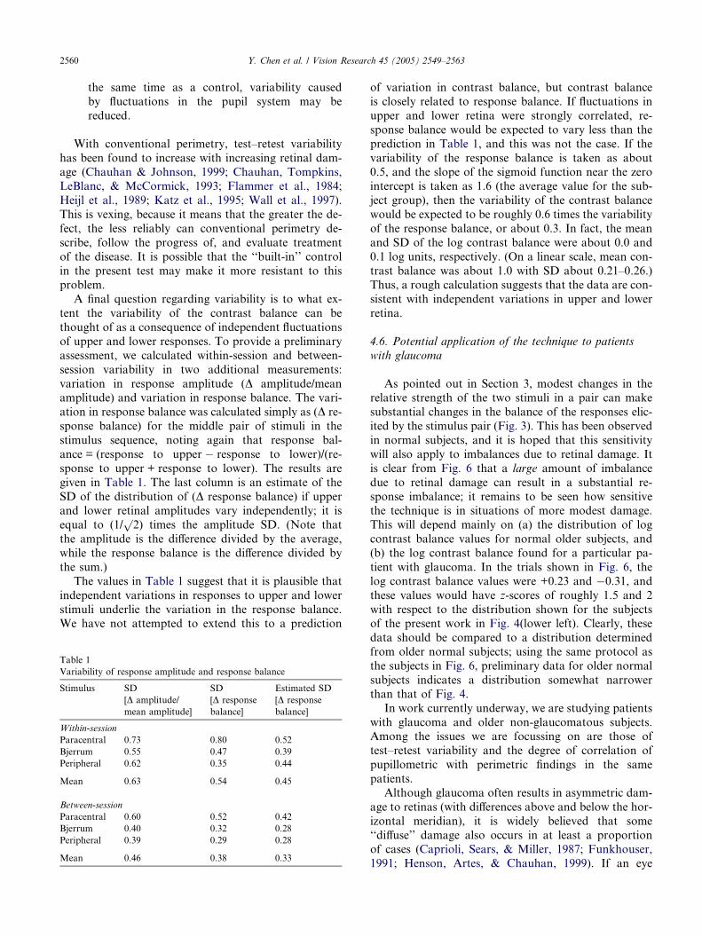
A final question regarding variability is to what ex-

tent the variability of the contrast balance can be

thought of as a consequence of independent fluctuations

of upper and lower responses. To provide a preliminary

assessment, we calculated within-session and between-

session variability in two additional measurements:

variation in response amplitude (D amplitude/meanamplitude) and variation in response balance. The vari-

ation in response balance was calculated simply as (D re-

sponse balance) for the middle pair of stimuli in the

stimulus sequence, noting again that response bal-

ance = (response to upper � response to lower)/(re-

sponse to upper + response to lower). The results are

given in Table 1. The last column is an estimate of the

SD of the distribution of (D response balance) if upperand lower retinal amplitudes vary independently; it is

equal to (1/p2) times the amplitude SD. (Note that

the amplitude is the difference divided by the average,

while the response balance is the difference divided by

the sum.)

The values in Table 1 suggest that it is plausible that

independent variations in responses to upper and lower

stimuli underlie the variation in the response balance.We have not attempted to extend this to a prediction

Table 1

Variability of response amplitude and response balance

Stimulus SD

[D amplitude/

mean amplitude]

SD

[D response

balance]

Estimated SD

[D response

balance]

Within-session

Paracentral 0.73 0.80 0.52

Bjerrum 0.55 0.47 0.39

Peripheral 0.62 0.35 0.44

Mean 0.63 0.54 0.45

Between-session

Paracentral 0.60 0.52 0.42

Bjerrum 0.40 0.32 0.28

Peripheral 0.39 0.29 0.28

Mean 0.46 0.38 0.33

of variation in contrast balance, but contrast balance

is closely related to response balance. If fluctuations in

upper and lower retina were strongly correlated, re-

sponse balance would be expected to vary less than the

prediction in Table 1, and this was not the case. If the

variability of the response balance is taken as about0.5, and the slope of the sigmoid function near the zero

intercept is taken as 1.6 (the average value for the sub-

ject group), then the variability of the contrast balance

would be expected to be roughly 0.6 times the variability

of the response balance, or about 0.3. In fact, the mean

and SD of the log contrast balance were about 0.0 and

0.1 log units, respectively. (On a linear scale, mean con-

trast balance was about 1.0 with SD about 0.21–0.26.)Thus, a rough calculation suggests that the data are con-

sistent with independent variations in upper and lower

retina.

4.6. Potential application of the technique to patients

with glaucoma

As pointed out in Section 3, modest changes in therelative strength of the two stimuli in a pair can make

substantial changes in the balance of the responses elic-

ited by the stimulus pair (Fig. 3). This has been observed

in normal subjects, and it is hoped that this sensitivity

will also apply to imbalances due to retinal damage. It

is clear from Fig. 6 that a large amount of imbalance

due to retinal damage can result in a substantial re-

sponse imbalance; it remains to be seen how sensitivethe technique is in situations of more modest damage.

This will depend mainly on (a) the distribution of log

contrast balance values for normal older subjects, and

(b) the log contrast balance found for a particular pa-

tient with glaucoma. In the trials shown in Fig. 6, the

log contrast balance values were +0.23 and �0.31, and

these values would have z-scores of roughly 1.5 and 2

with respect to the distribution shown for the subjectsof the present work in Fig. 4(lower left). Clearly, these

data should be compared to a distribution determined

from older normal subjects; using the same protocol as

the subjects in Fig. 6, preliminary data for older normal

subjects indicates a distribution somewhat narrower

than that of Fig. 4.

In work currently underway, we are studying patients

with glaucoma and older non-glaucomatous subjects.Among the issues we are focussing on are those of

test–retest variability and the degree of correlation of

pupillometric with perimetric findings in the same

patients.

Although glaucoma often results in asymmetric dam-

age to retinas (with differences above and below the hor-

izontal meridian), it is widely believed that some

‘‘diffuse’’ damage also occurs in at least a proportionof cases (Caprioli, Sears, & Miller, 1987; Funkhouser,

1991; Henson, Artes, & Chauhan, 1999). If an eye

Y. Chen et al. / Vision Research 45 (2005) 2549–2563 2561

suffered truly uniform damage, assessment of the con-

trast balance, as described in this paper, would not indi-

cate abnormality. For this reason, we have also been

studying the amplitudes of the responses to the stimuli

employed; in each trial, we have taken separate averages

of the three upper-stimulus response amplitudes and theaverages of the three lower-stimulus response ampli-

tudes. The amplitudes conform reasonably well to a

log normal distribution; i.e., the log amplitudes are nor-

mally distributed, with an SD of about 0.2–0.3 log units.

Preliminary analysis suggests that the amplitudes of the

responses can provide an additional method for assess-

ing the status of an eye. In work with patients and older

normal subjects, underway at present, we plan to assessthe effectiveness of such measures as well as the balance

measures.

4.7. Contrast balance vs. relative response amplitude

In developing the present technique, we considered

the use of relative response amplitude to a stimulus pair

of equal strength as the primary measure. Pilot experi-ments suggested that using contrast balance led to less

variability, and that measure was used. Contrast balance

is closer to a constant-criterion measure, such as a

threshold. The apparently greater stability may also

arise from the broader stimulus range employed in the

present approach. However, it is worth noting that the

greater speed of a test employing a relative response

measure might make it appropriate for situations inwhich speed is the critical factor, such as a screening

paradigm.

Acknowledgement

Supported by the Graduate Program in Vision Sci-

ence at SUNY State College of Optometry and NEIgrants R03EY014549 (HJW) and R01EY007716

(WHS).

Appendix A. Fitting sigmoid functions to response

balance data

This section describes, in more detail, the process fordetermining fits of sigmoid functions (Eq. (2)) to re-

sponse balance data from a trial.

Generally, both parameters of the function (slope ‘‘a’’

and contrast balance ‘‘x0’’) were allowed to vary to ob-

tain a best fitting sigmoid. This approach, which we call

a ‘‘free fit’’, was successful in fitting sigmoid functions to

the response balance data from most trials (e.g., Fig. 3).

In some cases, the free fit was not able to provide asuccessful fit, even though the data provided a clear indi-

cation of retinal function. For example, all three re-

sponse balance values were occasionally either negative

or positive, indicating a relatively weak pupil response

from superior or inferior retina. Free fits of sigmoid

functions were less reliable in such situations. Although

such an occurrence was rare in normal subjects, such sit-uations are more likely to occur in glaucoma patients,

where functional asymmetry between upper and lower

retina is expected. To deal with situations in which free

fits were unreliable, we developed a ‘‘constrained fitting’’

technique, in which the slope of the fitting function was

fixed at the mean value of successful free fits in the sub-

ject group, and only the contrast balance (x0) was al-

lowed to vary in Eq. (2). (This amounts to selectingthe average curve shape and sliding it along the x-axis

to find the best fit.)

There were several situations in which data from a

constrained fit were used for subsequent analysis: (1)

Data from a trial did not permit a free fit. (2) A free

fit gave a slope or contrast balance value (‘‘a’’ or

‘‘x0’’) outside a defined range. The defined range for

slope was taken as �0.5 to +5.0, which included mostof the ‘‘a’’ values found from successful free fits for indi-

vidual trials. The choice for the defined range of contrast

balance (x0) was based on the luminance range of the

stimuli in addition to the extrapolation range that was

believed to be reliable. From the stimulus luminance se-

quence used in the present study (24, 34, and 48 cd/m2),

we estimated a reasonable luminance range for extrapo-

lation to be 17–68 cd/m2. (The values 24, and 48 cd/m2are �0.15 and +0.15 log unit steps from the middle

luminance, respectively; a second 0.15 log unit step cor-

responds to 17 and 68 cd/m2, equivalent to an upper/

lower contrast range of �0.37 to +0.23 log units (the

lower stimulus luminance was 40 cd/m2)). The contrast

range allowed from free fits was finally set to be �0.35

to +0.35 log units for the present subject group, extend-

ing somewhat further than +0.23 log units in the positivedirection. This choice simplified processing and ap-

peared to be reasonable, based on careful examination

of the behavior of free fit data in the upper tail of the

distribution.

When a constrained fit gave an unusually large or

small contrast balance value, that value was ‘‘clipped’’

to a value outside which it was felt that numeric values

would be unreliable. The contrast range used to limitconstrained fits was �0.35 to +0.35 log units, the same

as used to shift from a free fit to a constrained fit. The

value that was assigned to the ‘‘clipped’’ data was

�0.40 or +0.40 log units, depending on which limit

was exceeded. This is a conservative approach, given

that the limits are much more likely to be exceeded for

patients with glaucoma than for normal subjects. It

was felt that it would be inappropriate to use specificnumerical values beyond the range of reasonably accu-

rate extrapolations.

2562 Y. Chen et al. / Vision Research 45 (2005) 2549–2563

Because the contrast balance for a trial is obtained

indirectly from the sigmoid curve fitted to the trial data,

it was of interest to know how well the sigmoid fitted the

data. In the present study, the square root of mean

squared deviation (SRMSD) of the fitted curve to the re-

sponse balance data was used as a measure of fit quality.SRMSD is similar to standard deviation for a one-

dimensional distribution.

SRMSD¼

ffiffiffiffiffiffiffiffiffiffiffiffiffiffiffiffiffiffiffiffiffiffiffiffiffiffiffiffiffiffiffiffiffiffiffiffiffiffiffiffiffiffiffiffiffiffiffiffiffiffiffiffiffiffiffiffiffiffiffiffiffiffiffiffiffiffiffiffiffiffiffiffiffiffiffiffiffiffiffiffiffiffiffiffiffiffiffiffiffiffiðR1�F ðL1ÞÞ2þðR2�F ðL2ÞÞ2þðR3�F ðL3ÞÞ2

3

s

ð3Þ

Ri: i = 1, 2, 3, response balance obtained from raw

data;

F(Li): i = 1, 2, 3, sigmoid function at each contrastlevel.

When the distribution of SRMSD�s was examined for

free fits to data from all individual trials for which it was

possible to carry out free fits, 97.2% were smaller than

0.5. Based on this, it was decided to reject data from tri-

als for which both free and constrained fits gave

SRMSD�s greater than 0.5. For the subjects in the pres-ent work, these criteria gave a data rejection rate of 7%

of all individual trials.

It should be stressed that it was rare that data from

normal subjects were clipped or rejected due to large

SRMSD values. We were interested in setting up a gen-

eral protocol for data analysis that could be applied to

data from patients as well as data from normal subjects.

Thus, clipping would tend to narrow the distribution ofdata from abnormal retinas much more frequently than

it would affect the distribution from normal retinas. This

is an appropriately conservative position, making it more

difficult for patients� data to fall at large distances from

the center of the distribution of normal subjects� data.

References

Asman, P., & Heijl, A. (1992a). Evaluation of methods for automated

Hemifield analysis in perimetry. Archives of Ophthalmology, 110(6),

820–826.

Asman, P., & Heijl, A. (1992b). Glaucoma Hemifield Test. Automated

visual field evaluation. Archives of Ophthalmology, 110(6), 812–819.

Aulhorn, E., & Karmeyer, H. (1977). Frequency distribution in early

glaucomatous visual field defects. In E. L. Greve (Ed.). Documen-

tal ophthalmologica proc. ser. 14 (pp. 75–83). The Hague: Dr. W.

Junk bv Publishers.

Bengtsson, B., & Heijl, A. (1998). SITA Fast, a new rapid perimetric

threshold test. Description of methods and evaluation in patients

with manifest and suspect glaucoma. Acta Ophthalmologica Scan-

dinavica, 76, 431–437.

Bengtsson, B., Heijl, A., & Olsson, J. (1998). Evaluation of a new

threshold visual field strategy, SITA, in normal subjects. Swedish

Interactive Thresholding Algorithm. Acta Ophthalmologica Scan-

dinavica, 76, 165–169.

Bland, J. M., & Altman, D. G. (2003). Applying the right statistics:

Analysis of measurement studies. Ultrasound in Obstetrics and

Gynecology, 22, 85–93.

Bouma, H. (1965). Receptive systems: Mediating certain light reactions

of the pupil of the human eye (p. 112–160). Eindhoven, Nether-

lands: Philips Research Reports Supplements.

Brainard, D. H. (1997). The Psychophysics Toolbox. Spatial Vision,

10, 433–436.

Caprioli, J., Sears, M., & Miller, J. M. (1987). Patterns of early visual

field loss in open-angle glaucoma. American Journal of Ophthal-

mology, 103, 512–517.

Chauhan, B. C., & Johnson, C. A. (1999). Test–retest variability of

frequency-doubling perimetry and conventional perimetry in glau-

coma patients and normal subjects. Investigative Ophthalmology

and Visual Science, 40(3), 648–656.

Chauhan, B. C., Tompkins, J. D., LeBlanc, R. P., & McCormick, T. A.

(1993). Characteristics of frequency-of-seeing curves in normal

subjects, patients with suspected glaucoma, and patients with

glaucoma. Investigative Ophthalmology and Visual Science, 34(13),

3534–3540.

Choplin, N. T., & Edwards, R. P. (1995). Visual field testing with the

Humphrey Field Analyzer. Thorofare, NJ: SLACK Inc.

Clarke, R. J., Zhang, H., & Gamlin, P. D. (2003a). Characteristics of

the pupillary light reflex in the alert rhesus monkey. Journal of

Neurophysiology, 89(6), 3179–3189.

Clarke, R. J., Zhang, H., & Gamlin, P. D. (2003b). Primate pupillary

light reflex: Receptive field characteristics of pretectal luminance

neurons. Journal of Neurophysiology, 89(6), 3168–3178.

Fankhauser, F., & Flammer, J. (1989). Puptrak 1.0—a new semiau-

tomated system for pupillometry with the Octopus perimeter: A

preliminary report. Documenta Ophthalmologica, 73(3), 235–248.

Felius, J., Swanson, W. H., Fellman, R. L., Lynn, J. R., & Starita, R.

J. (1996). Spatial summation for selected ganglion cell mosaics in

patients with glaucoma. In M. Wall & A. Heijl (Eds.), Perimetry

update 1996/1997 (pp. 213–221). Wurzburg, Germany: Kugler

Publications.

Flammer, J., Drance, S. M., & Zulauf, M. (1984). Differential light

threshold. Short- and long-term fluctuation in patients with

glaucoma, normal controls, and patients with suspected glaucoma.

Archives of Ophthalmology, 102(5), 704–706.

Funkhouser, A. T. (1991). A new diffuse loss index for estimating

general glaucomatous visual field depression. Documenta Ophthal-

mologica, 77(1), 57–72.

Gamlin, P. D., Zhang, H., & Clarke, R. J. (1995). Luminance neurons

in the pretectal olivary nucleus mediate the pupillary light reflex in

the rhesus monkey. Experimental Brain Research, 106(1), 169–176.

Gilpin, L. B., Stewart, W. C., Hunt, H. H., & Broom, C. D. (1990).

Threshold variability using different Goldmann stimulus sizes. Acta

Ophthalmologica (Copenh), 68(6), 674–676.

Hart, W. M., Jr., & Becker, B. (1982). The onset and evolution of

glaucomatous visual field defects. Ophthalmology, 89(3), 268–279.

Heijl, A., Lindgren, A., & Lindgren, G. (1989). Test–retest variability

in glaucomatous visual fields. American Journal of Ophthalmology,

108(2), 130–135.

Heijl, A., Lindgren, G., & Olsson, J. (1987). Normal variability of

static perimetric threshold values across the central visual field.

Archives of Ophthalmology, 105(11), 1544–1549.

Heijl, A., & Lundqvist, L. (1984). The frequency distribution of earliest

glaucomatous visual field defects documented by automatic

perimetry. Acta Ophthalmologica (Copenh), 62(4), 658–664.

Henson, D. B., Artes, P. H., & Chauhan, B. C. (1999). Diffuse loss of

sensitivity in early glaucoma. Investigative Ophthalmology and

Visual Science, 40(13), 3147–3151.

Hong, S., Narkiewicz, J., & Kardon, R. H. (2001). Comparison of

pupil perimetry and visual perimetry in normal eyes: Decibel

sensitivity and variability. Investigative Ophthalmology and Visual

Science, 42(5), 957–965.

Y. Chen et al. / Vision Research 45 (2005) 2549–2563 2563

Hood, D. C., Thienprasiddhi, P., Greenstein, V. C., Winn, B. J., Ohri,

N., Liebmann, J. M., et al. (2004). Detecting early to mild

glaucomatous damage: A comparison of the multifocal VEP and

automated perimetry. Investigative Ophthalmology and Visual

Science, 45(2), 492–498.

Hultborn, H., Mori, K., & Tsukahara, N. (1978). The neuronal

pathway subserving the pupillary light reflex. Brain Research,

159(2), 255–267.

Johnson, L. N., Hill, R. A., & Bartholomew, M. J. (1988). Correlation

of afferent pupillary defect with visual field loss on automated

perimetry. Ophthalmology, 95(12), 1649–1655.

Kardon, R. H. (1992). Pupil perimetry. Current Opinion in Ophthal-

mology, 3(5), 565–570.

Kardon, R. H., Kirkali, P. A., & Thompson, H. S. (1991). Automated

pupil perimetry. Pupil field mapping in patients and normal

subjects. Ophthalmology, 98(4), 485–495.

Kardon, R. H., & Thompson, H. S. (1994). Pupil perimetry: Methods

of threshold determination and comparison with visual response.

In R. P. Mills & M. Wall (Eds.), Perimetry update 1994/1995

(pp. 119–123). Washington DC, USA, Amsterdam/New York:

Kugler Publications.

Katz, J., Quigley, H. A., & Sommer, A. (1995). Repeatability of the

Glaucoma Hemifield Test in automated perimetry. Investigative

Ophthalmology and Visual Science, 36(8), 1658–1664.

Krill, A. E., Smith, V. C., Blough, R., & Pass, A. (1968). An absolute

threshold defect in the inferior retina. Investigative Ophthalmology,

7(6), 701–707.

Lagreze, W. D., & Kardon, R. H. (1998). Correlation of relative

afferent pupillary defect and estimated retinal ganglion cell loss.

Graefes Archive for Clinical and Experimental Ophthalmology,

236(6), 401–404.

Levatin, P. (1959). Pupillary escape in disease of the retina or optic

nerve. Archives of Ophthalmology, 62, 768–779.

Loewenfeld, I. E., & Rosskothen, H. D. (1974). Infrared pupil camera.

A new method for mass screening and clinical use. American

Journal of Ophthalmology, 78(2), 304–313.

Lowenstein, O., Kawabata, H., & Loewenfeld, I. E. (1964). The pupil

as indicator of retinal activity. American Journal of Ophthalmology,

57, 569–596.

Lowenstein, O., & Loewenfeld, I. E. (1969). The pupil. In H. Davson

(Ed.), The eye (pp. 255–337). New York: Academic Press.

Lucas, R. J., Hattar, S., Takao, M., Berson, D. M., Foster, R. G., &

Yau, K. W. (2003). Diminished pupillary light reflex at high

irradiances in melanopsin-knockout mice. Science, 299(5604),

245–247.

Pearson, P., Swanson, W. H., & Fellman, R. L. (2001). Chromatic and

achromatic defects in patients with progressing glaucoma. Vision

Research, 41(9), 1215–1227.

Pelli, D. G. (1997). The VideoToolbox software for visual psycho-

physics: transforming numbers into movies. Spatial Vision, 10,

437–442.

Perry, V. H., & Cowey, A. (1984). Retinal ganglion cells that project to

the superior colliculus and pretectum in the macaque monkey.

Neuroscience, 12(4), 1125–1137.

Rodieck, R. (1998). Informing the brain. In The first steps in

seeing (pp. 276–279). Sunderland, MA: Sinauer Associates, Inc.

Publisher.

Sample, P. A., Irak, I., Martinez, G. A., & Yamagishi, N. (1997).

Asymmetries in the normal short-wavelength visual field: Implica-

tions for short-wavelength automated perimetry. American Journal

of Ophthalmology, 124(1), 46–52.

Schweitzer, N. M. J., & Bouman, M. A. (1957). Differential threshold

measurements on the light reflex of the human pupil. A.M.A.Arc-

hives of Ophthalmology, 59, 541–550.

Skrandies, W. (1987). The upper and lower visual field of man:

Electrophysiological and functional differences. In D. Ottoson

(Ed.). Sensory physiology (8, pp. 48–93). Berlin, Heidelberg, New

York, London, Paris, Tokyo: Springer-Verlag.

Stark, L. (1969). Pupillary control system: Its nonlinear adaptive and

stochastic engineering design characteristics. Federation Proceed-

ings, 28(1), 52–64.

Thompson, H. S. (1975). The pupil. In W. M. Hart, Jr. (Ed.), Adler�sphysiology of the eye (pp. 412–441). St. Louis, Baltimore, Boston,

Chicago, London, Philadelphia, Sydney, Toronto: Mosby-Year

Book, Inc.

Thompson, H. S., Montague, P., Cox, T. A., & Corbett, J. J. (1982).

The relationship between visual acuity, pupillary defect, and visual

field loss. American Journal of Ophthalmology, 93(6), 681–688.

Trejo, L. J., & Cicerone, C. M. (1984). Cells in the pretectal olivary

nucleus are in the pathway for the direct light reflex of the pupil in

the rat. Brain Research, 300(1), 49–62.

Turtschi, S., Bergamin, O., Dubler, B., Schotzau, A., & Zulauf, M.

(1994). Pupillenperimetrie mit dem OCTOPUS 1-2-3. Erste Erfahr-

ungen. Klinische Monatsblatter fur Augenheilkunde, 204(5),

398–399.

Ukai, K. (1985). Spatial pattern as a stimulus to the pupillary system.

Journal of the Optical Society of America A–Optics Image Science

and Vision, 2(7), 1094–1100.

Vrabec, F. (1966). The temporal raphe of the human retina. American

Journal of Ophthalmology, 62(5), 926–938.

Wall, M., Kutzko, K. E., & Chauhan, B. C. (1997). Variability in

patients with glaucomatous visual field damage is reduced using

size V stimuli. Investigative Ophthalmology and Visual Science,

38(2), 426–435.

Weber, J., & Ulrich, H. (1987). Die exakte Localisation der Nervenfa-

seraquivalenten Linien im Gesichtsfeld. Fortschritte der Ophthal-

mologic (Berlin), 84(1), 101–103.

Weber, J., & Ulrich, H. (1991). A perimetric nerve fiber bundle map.

International Journal of Ophthalmology, 15(3), 193–200.

Wilhelm, H., Neitzel, J., Wilhelm, B., Beuel, S., Ludtke, H., Kretsch-

mann, U., et al. (2000). Pupil perimetry using M-sequence stim-

ulation technique. Investigative Ophthalmology and Visual Science,

41(5), 1229–1238.

Wyatt, H. J. (1992). Clinical research note: A hypothesis concerning

the relationship between retinotopy in the optic nerve head and

perimetry. Clinical Vision Sciences, 7(2), 153–161.

Wyatt, H. J., & Musselman, J. F. (1981). Pupillary light reflex in

humans: Evidence for an unbalanced pathway from nasal retina,

and for signal cancellation in brainstem. Vision Research, 21(4),

513–525.

Yoshitomi, T., Matsui, T., Tanakadate, A., & Ishikawa, S. (1999).

Comparison of threshold visual perimetry and objective pupil

perimetry in clinical patients. Journal of Neuroophthalmology,

19(2), 89–99.