pure and applied sciences - covenant...
TRANSCRIPT


EDITORMZ Khan, SENRA Academic PublishersBurnaby, British Columbia, Canada
ASSOCIATE EDITORSDongmei Zhou, Institute of Soil ScienceChines Academy of Sciences, China
Errol Hassan, University of QueenslandGatton, Australia
Paul CH Li, Simon Fraser UniversityBurnaby, British Columbia, Canada
EDITORIAL STAFFJasen NelsonWalter LeungSara AliHao-Feng (howie) LaiBen ShiehAlvin Louie
MANAGING DIRECTORMak, SENRA Academic PublishersBurnaby, British Columbia, Canada
Board of Editorial Advisors
Richard CallaghanUniversity of Calgary, AB, CanadaDavid T CrambUniversity of Calgary, AB, CanadaMatthew CooperGrand Valley State University, AWRI, Muskegon, MI, USAAnatoly S BorisovKazan State University, Tatarstan, RussiaRon ColeyColey Water Resource & Environment Consultants, MB, CanadaChia-Chu ChiangUniversity of Arkansas at Little Rock, Arkansas, USAMichael J DreslikIllinois Natural History, Champaign, IL, USADavid FederUniversity of Calgary, AB, CanadaDavid M GardinerUniversity of California, Irvine, CA, USAGeoffrey J HayUniversity of Calgary, AB, CanadaChen HaoanGuangdong Institute for drug control, Guangzhou, ChinaHiroyoshi ArigaHokkaido University, JapanGongzhu HuCentral Michigan University, Mount Pleasant, MI, USAMoshe InbarUniversity of Haifa at Qranim, Tivon, IsraelSA IsiorhoIndiana University - Purdue University, (IPFW), IN, USABor-Luh LinUniversity of Iowa, IA, USAJinfei LiGuangdong Coastal Institute for Drug Control, Guangzhou, ChinaCollen KellyVictoria University of Wellington, New ZealandHamid M.K.AL-NaimiyUniversity of Sharjah, UAEEric L PetersChicago State University, Chicago, IL, USARoustam LatypovKazan State University, Kazan, RussiaFrances CP LawSimon Fraser University, Burnaby, BC, CanadaGuangchun LeiRamsar Convention Secretariat, SwitzerlandAtif M MemonUniversity of Maryland, MD, USASR NasyrovKazan State University,Kazan, RussiaRussell A NicholsonSimon Fraser University, Burnaby, BC, CanadaBorislava GutartsCalifornia State University, CA, USASally PowerImperial College London, UK
Volume 7, Number 3Oct. 2013
Editorial OfficeE-mail: [email protected]
The Canadian Journal of Pure and AppliedSciences (CJPAS-ISSN 1715-9997) is a peerreviewed multi-disciplinary specialist journalaimed at promoting research worldwide inAgricultural Sciences, Biological Sciences,Chemical Sciences, Computer and MathematicalSciences, Engineering, Environmental Sciences,Medicine and Physics (al l subjects).
Every effort is made by the editors, board ofeditorial advisors and publishers to see that noinaccurate or misleading data, opinions, orstatements appear in this journal, they wish tomake clear that data and opinions appearingin the articles are the sole responsibility of thecontributor concerned. The CJPAS accept noresponsibility for the misleading data, opinionor statements.
5919 129 B Street SurreyBritish Columbia V3X 0C5 Canadawww.cjpas.netE-mail: [email protected]
Academic PublishersSENRA
Print ISSN 1715-9997Online ISSN 1920-3853
CJPAS is Abstracted/Indexed in:
CANADIAN JOURNAL OFPURE AND APPLIED SCIENCES
MemberCANADIAN ASSOCIATION OF LEARNED JOURNALS
Gordon McGregor ReidNorth of England Zoological Society, UKPratim K ChattarajIndian Institute of Technology, Kharagpur, IndiaAndrew Alek TuenInstitute of Biodiversity, Universiti Malaysia Sarawak, MalaysiaDale WrubleskiInstitute for Wetland and Waterfowl Research, Stonewall, MB, CanadaDietrich Schmidt-VogtAsian Institute of Technology, ThailandDiganta GoswamiIndian Institute of Technology Guwahati, Assam, IndiaM Iqbal ChoudharyHEJ Research Institute of Chemistry, KarachiDaniel Z SuiTexas A&M University, TX, USASS AlamIndian Institute of Technology Kharagpur, IndiaBiagio RicceriUniversity of Catania, ItalyZhang HemingChemistry & Environment College, Normal University, ChinaC VisvanathanAsian Institute of Technology, ThailandIndraneil DasUniversiti Malaysia, Sarawak, MalaysiaGopal DasIndian Institute of Technology , Guwahati, IndiaMelanie LJ StiassnyAmerican Museum of Natural History, New York, NY, USAKumlesh K DevBio-Sciences Research Institute, University College Cork, Ireland.Shakeel A KhanUniversity of Karachi, KarachiXiaobin ShenUniversity of Melbourne, AustraliaMaria V KalevitchRobert Morris University, PA, USAXing JinHong Kong University of Science & Tech.Leszek CzuchajowskiUniversity of Idaho, ID, USABasem S AttiliUAE University, UAEDavid K ChiuUniversity of Guelph, Ontario, CanadaGustavo DavicoUniversity of Idaho, ID, USAAndrew V SillsGeorgia Southern University Statesboro, GA, USACharles S. WongUniversity of Alberta, CanadaGreg GastonUniversity of North Alabama, USA
Thomson Reuters, EBSCO, Ulrich'sPeriodicals Directory, Scirus, CiteSeerX,Index Copernicus, Directory of OpenAccess Journals, Google Scholar, CABI,Chemical Abstracts, Zoological Records,Global Impact Factor Australia, J-Gate,HINARI, WorldCat, British Library,European Library, Biblioteca Central, TheI n t u t e Conso r t i um, Genam icsJournalSeek, bibliotek.dk, OAJSE, ZurichOpen Repository and Archive JournalDatabase. CJPAS has received:
Global Impact Factor for 2012 = 2.657Index Copernicus Journals Evaluation for2011 = 4.63Frequency:3 times a year (Feb, June and Oct.)

Volume 7, Number 3 October 2013
CONTENTS
LIFE SCIENCES Omar Sarheed Combination Treatments of Chemical Enhancers with Low Frequency Ultrasound for the Transdermal Delivery of Hydrocortisone ..................................................................................................................................... 2463 Zafar Iqbal and Rod Wootten Population Biology of a Cestode, Proteocephalus filicollis (Rudolphi) from Gasterosteus aculeatus L. in Scotland ............................................................................................................................................................... 2475 MAA Mamun, MM Rana and AJ Mridha Tray Soil Management in Raising Seedlings for Rice Transplanter ........................................................................ 2481 Muhammad Sheeraz Ahmad, S M Saqlan Naqvi, Sajida Mushtaq, Farzana Ramzan, Abdul Sami, Salma Batool, Ihsan-ul-Haq and Bushra Mirza Phytochemical and Biological Evaluation of Polygonum amplexicaule Rhizome Extract ...................................... 2491
R Kurma Rao and K Ramesh Babu Studies on Food and Feeding Habits of Mugil Cephalus (Linnaeus, 1758) East Coast Off Andhra Pradesh, India ............................................................................................................................................. 2499 Riffat Sultana, Yawar S Wagan, M Naeem, M Saeed Wagan and Imran Khatri Systematic Studies and Host Specificity of Scelio (Hymenoptera: Sceliondae) Egg Parasitoids of Orthoptera from Pakistan ........................................................................................................................................................... 2505 Syed A Ghalib, Saquib E Hussain, M Zaheer Khan, Said A Damhoureyeh, Rehana Yasmeen, Afsheen Zehra, Farina Fatima, Babar Hussain, Saima Siddiqui, Darakhshan Abbas, Fozia Tabbassum, Naseem Samreen, A Razzaq Khan, Tanveer Jabeen, M Usman A Hashmi and Syed Ali Hasnain An Overview of Occurrence, Distribution and Status of the Birds of Khirthar Protected Area Complex (KPAC), Sindh ........................................................................................................................................................ 2515 Short Communications
Oladipo GS, Okoh PD and Yorkum KL The Frequency of Ocular Dominance in the Okrikas and Ikwerres of Nigeria ....................................................... 2533
Isehunwa O Grace and Alada AR Akinola Seasonal and Sex Variation in the Blood Parameters of the Common African Toad Bufo regularis ...................... 2537 Iman Bajalan, Mehrdad Akbarzadeh , Esmail Qalayi and Elahe Yarahmadi Comparison of Chemical Compition of Essential Oil of Mentha longifolia L. from two Regions of Iran .............. 2541
Scientific Note Anita Jacob and M Haridas An Endophyte, Reversing MDR in Pseudomonas Strain ........................................................................................ 2545

PHYSICAL SCIENCES AE Pillay, S Stephen, A Abd-Elhameed and JR Williams Rapid Liquid Nitrogen Pre-treatment of Gels, Waxes and Pastes for Deep-UV Depth-Profiling Studies (ICP-MS) .................................................................................................................................................... 2549 A A Zakharenko New Nondispersive Sh-Saws Guided by the Surface of Piezoelectromagnetics ..................................................... 2557
Boateng Ampadu, Nick A Chappell and Raymond A Kasei Rainfall-Riverflow Modelling Approaches: Making a Choice of Data-Based Mechanistic Modelling Approach for Data Limited Catchments: A Review ................................................................................................ 2571 Gabriel Y. H. Avossevou Group Theory and Harmonic Oscillators in the Plane ............................................................................................. 2581
Okeniyi JO, Okpala SO, Omoniyi OM, Oladele IO, Ambrose IJ, Menkiti MC, Loto CA and Popoola API Methods of Astm G16 and Conflicts in Corrosion Test Data: Case Study of Nano2 Effectiveness on Steel-Rebar Corrosion ........................................................................................................................................ 2589
Haji Muhammad, Zafar Iqbal, Muhammad Ayub and M Anwar Malik Uptake of Heavy Metals by Brassica compestris, Irrigated by Hudiara Drain in Lahore, Pakistan ........................ 2599
Awodugba AO and Araromi DO Multiobjective Optimization (MO) of Chemical Bath Deposition Process for CDS Thin Film using Genetic Algorithm ................................................................................................................................................................ 2605 Muhammad Asif Khan An Integrated Framework to Bridging the Gap Between Business and Information Technology – A Co-Evolutionary Approach .................................................................................................................................. 2611 Ogunniran, KO, Adekoya, JA, Siyanbola, TO, Ajayeoba, TA and Inegbenebor, AI Synthesis, Antibacterial and Toxicology Study of MN(II), Co(II) and Ni(II) Metal Complexes of Sulfadoxine Mixed with Pyrimethamine ..................................................................................................................................... 2619 Short Communications Maria V Kalevitch, Paul Badger, Bill Dress and Valentine I Kefeli Elemental Content of Manufactured Soils ............................................................................................................... 2629 Awodugba Ayodeji Oladiran and Ilyas Abdul-Mojeed Olabisi Fabrication Of Dye Sensitized Solar Cell (DSSC) using ZnO Nanoparticles Synthesized From Zinc Nitrate Hexahydrate ............................................................................................................................................................. 2635 Egwali Annie O and Akwukwuma V V N AN-VE: An Improved Hamming Coding Technique .............................................................................................. 2639 S B Akpila Predictive Models on Settlement Parameters of Clayey Soils: A Case Study in Port-Harcourt City of Nigeria .... 2649 Badal H Elias, Saad F Ramadhan and Dunia D Giliyana The Effect of Noise Pollution on School Children at Duhok City, Iraq .................................................................. 2655

SENRA Academic Publishers, British Columbia Vol. 7, No. 3, pp. 2463-2473, October 2013 Online ISSN: 1920-3853; Print ISSN: 1715-9997
COMBINATION TREATMENTS OF CHEMICAL ENHANCERS WITH LOW FREQUENCY ULTRASOUND FOR THE TRANSDERMAL DELIVERY OF
HYDROCORTISONE
*Omar Sarheed Strathclyde Institute of Pharmacy and Biomedical Sciences, University of Strathclyde
27 Taylor Street, Glasgow G4 0NR, Scotland, UK
ABSTRACT The aim of this study was to investigate combination treatments of chemical enhancers and 20 kHz ultrasound across porcine skin in order to identify possible synergistic and/or additive effects. For this purpose, three different classes of permeation enhancers were selected. These were: terpenes, fatty acids and sodium lauryl sulphate (a surfactant). Terpenes were chosen as their low cutaneous irritancy makes them attractive for clinical use. Fatty acids were chosen due to their general potency, widespread historical use and established status as dermal enhancers. Sodium lauryl sulphate was chosen as it has already been proven to act synergistically with low frequency ultrasound. Throughout, hydrocortisone was used as a model drug screen the selected ultrasound application with various chemical enhancer pre-treatments. The 300s concurrently-applied beam, at a 10% duty cycle was used as an application protocol for the study. Synergism with menthone and sodium lauryl sulphate occurred. More interesting was the fact that ultrasound exposure following 1% SLS treatment caused a highly significant synergistic 8.8-fold increase in hydrocortisone delivery. Treatment with 0.25% SLS and ultrasound caused a significant additive effect. A simultaneous administration of all three treatments could be more effective and probably simpler to apply to hydrocortisone compared with passive transdermal delivery. Keywords: Sonophoresis, chemical enhancers, low frequency ultrasound, transdermal, skin permeation, hydrocortisone. INTRODUCTION Terpenes are naturally occurring volatile oils that have been tested fairly extensively as percutaneous chemical enhancers (Vaddi et al., 2002; Williams and Barry, 2004). Although these compounds can exhibit good transdermal enhancement ability, they usually cause only low cutaneous irritancy. Hence, terpenes have been given the designation of “generally recognized as safe” (GRAS) by the Food and Drug Administration (FDA) (Godwin and Michniak, 1999; Asbill and Michniak, 2000). Application of differential scanning calorimetry, X-ray diffraction and infra-red techniques have shown that the terpenes act at least in part by modifying the intercellular lipids of the stratum corneum and disrupting their highly ordered structure (El-Kattan et al., 2001). Differential scanning calorimetry research on hydrated stratum corneum samples showed that applied 1, 8-cineole did in fact act in this way (Cornwell and Barry, 1993). Narishetty and Panchagnula (2004) chose 1, 8-cineole, menthol, α-terpineol and (+)-carvone and studied the effects of each of these oxygen-containing terpenes on zidovudine permeation across rat skin in vitro. All of these terpenes significantly increased the transdermal flux of the hydrophilic drug. Molecular modelling showed that
terpene molecules probably hydrogen bond with intercellular lipid head groups of the stratum corneum. This disrupts the pre-existing interlamellar hydrogen bonding network and increases the distance between two opposite lamellae. This effectively creates new polar pathways or channels through the stratum corneum barrier. Terpenes seem to be more effective as enhancers when they are formulated in propylene glycol (Vaddi et al., 2002). Over the years, many terpene studies have been performed in order to rationalise the selection of the best terpene for any specific percutaneously applied drug. Okabe and co-authors (Okabe et al., 1989) studied ten different cyclic monoterpenes. They reported that terpenes with lipophilic indices greater than zero were most effective at enhancing indomethacin delivery in vitro. In general, it appears that lipophilic terpenes such as the hydrocarbons tend to be effective for promoting the absorption of lipophilic drugs. In contrast, more hydrophilic oxygen-containing terpenes such as alcohols and ketones are effective for promoting the absorption of hydrophilic drugs (Williams and Barry, 2004; Hori et al., 1991; Williams and Barry, 1991a; Williams and Barry, 1991b; Fang et al., 2007).
Corresponding author Present address: RAK College of Pharmaceutical Sciences, RAK Medical and Health Sciences University, Ras Al Khaimah, United Arab Emirates. Email: [email protected]

Sarheed 2464
Up to our knowledge there seems to be one literature report by Mutalik et al. (2009) dealing with the combined effect of terpenes and low frequency ultrasound on transdermal drug absorption using full thickness mouse skin which is generally more permeable than human skin due to a high density of hair follicles as well as other structural and biochemical differences (Walters and Roberts, 1993). The GRAS status of terpenes means that they probably would be good candidates for combined use with sonophoresis if the treatments acted synergistically. In order to explore this idea, four monocyclic terpenes were selected for use in the sonophoresis studies. These were (+)-carvone, 1,8-cineole, menthone and α-terpineol. It is interesting to note that three of these are chemically-distinct structural isomers -1,8-cineole (an ether), α-terpineol (an alcohol), and menthone (a ketone). These three terpene molecules have a molecular weight of 154 Da. (+)-carvone is also a ketone but with a molecular weight of 150 Da. All four of these hydrophilic terpenes have a free hydroxyl or oxygen group and so they should be able to perturb stratum corneum lipid packing through the formation of hydrogen bonds (Vaddi et al., 2002; Fang et al., 2007). All four terpenes have a similar density of ∼0.9 g/ml. Fatty acids are one the most extensive studied group of transdermal permeation enhancers (Wang et al., 2004). It is known that these enhancers act by disrupting intercellular lipid packing in the stratum corneum, allowing any applied drug to more readily permeate through the layer. The exact mechanisms are not yet fully understood. It is possible that certain fatty acids can extract a fraction of the endogenous stratum corneum membrane components, causing phase separation to occur. This will lower the proportion of crystalline lipids and create more permeable fatty acid-rich domains (Rowat et al., 2006). Chemically, fatty acids consist of an aliphatic hydrocarbon chain and a terminal carboxyl group. They differ from each other in various parameters such as hydrocarbon chain length as well as the number, position and configuration of double bonds. Other differences include the extent of hydrocarbon chain branching or the presence of additional functional groups. The enhancer potency of a fatty acid is known to be related to these molecular properties. For saturated fatty acids, a hydrophobic chain length of about 12 carbon atoms was found to be optimal, generally possessing an optimal balance between partition coefficient, solubility parameter and affinity to skin (Aungst et al., 1986; Aungst, 1989; Elyan et al., 1996). For unsaturated fatty acids, chain lengths of about 18 carbon atoms appear to be the best (Williams and Barry, 2004). The presence of double bonds will affect the efficiency of fatty acids as chemical enhancers. It is well established that unsaturated fatty acids are usually more potent than saturated ones in permeating the skin and
facilitating enhanced drug delivery (Aungst et al., 1986; Bhatia and Singh, 1998). It is important to note that the fatty acids are usually formulated in a propylene glycol vehicle. This allows the so-called “solvent drag mechanism” to take place (Wang et al., 2004; Aungst et al., 1990) causing better skin penetration of both the fatty acid and the vehicle. In a study by Cotte et al. (2004), it was reported that myristic acid was able to penetrate deeper into epidermal layers of the skin when propylene glycol was used as the vehicle. Deeper penetration of the fatty acid leads to improved enhancer activity. Importantly, propylene glycol is widely used in topical formulations (Ho et al., 1998) because of its low toxicity to the skin (Fang et al., 2003). The aim in the present study was to explore the combination treatment of each of three fatty acids with low frequency ultrasound. The fatty acid molecules chosen were; oleic acid, linoleic acid and stearic acid. It can be seen that all three molecules have the same chain length of 18 carbons but differ in the number of double bonds. Linoleic, oleic and stearic acids have two, one and zero double bonds, respectively. Sodium lauryl sulphate is also of particular interest in relation to sonophoresis as it has already been shown to act synergistically with low frequency ultrasound in permeabilising the skin barrier. Mitragotri et al. (2000) studied the combining effect of 20 kHz ultrasound with SLS in an in vitro full thickness porcine skin model. It was determined that treatment with SLS alone as well as ultrasound alone both increased the skin permeability of mannitol. Application of SLS alone for 90 minutes produced an approximate 3-fold increase in mannitol permeation, while application of ultrasound alone for 90 min produced an approximate 8-fold enhancement. In the present study, SLS and 20 kHz ultrasound effects were investigated with in vitro transport studies, using hydrocortisone as a model drug. MATERIALS AND METHODS Materials menthone, 1,8-cineole, α-terpineol, (+)-carvone, linoleic acid, oleic acid, stearic acid, sodium lauryl sulphate (SLS), hydrocortisone and propylene glycol were purchased from Sigma-Aldrich (Poole, UK). Phosphate buffer saline tablets (pH 7.4), potassium dihydrogen orthophosphate and disodium hydrogen orthophosphate were purchased from Sigma-Aldrich (Poole, UK). [1,2,6,7-3H]-hydrocortisone (74 Ci/mmol) was purchased from Amersham Biosciences (Buckinghamshire, UK). Scintillation fluid (Optiphase HiSafe 3) and scintillation vials were purchased from Fisher Scientific (Loughborough, UK) and Packard Instrument Co. (Meriden, CT), respectively. Double distilled, de-ionised water was employed throughout.

Canadian Journal of Pure and Applied Sciences 2465
Transport studies Preparation of donor and receiver solutions A degassed PBS solution (pH=7.4) was prepared by taking five tablets of PBS tablets and dissolving those in 1 L of double-distilled water to form a solution with a; phosphate concentration of 0.01 M, potassium chloride concentration of 0.0027 M and sodium chloride concentration of 0.137 M. The pH was 7.4. This was used as the receiver fluid in all the studies described in this chapter. A 10 mg mass of hydrocortisone powder was weighed out and dissolved in 100 ml of PBS to form a 0.01% (w/v) solution. A suitable small volume of tritiated hydrocortisone was added and mixed in to form a solution exhibiting an activity of 1 µCi/ml. This was used as the donor solution for the studies. Preparation of full-thickness skin samples Porcine ears (Landrace species) were obtained immediately after slaughter from a local abattoir but before steam sterilisation of the tissue. The skins were cleaned under cold running water. The external surface of each ear was sectioned horizontally by scalpel to yield whole skin samples of area ∼8 cm2. The skin sections were visually checked for integrity and then stored in a frozen state (-20°C) for a maximum period of 3 months. Immediately prior to the permeation studies, the porcine skin sections were thawed at room temperature and cut into smaller samples of surface area ∼1 cm2. These skin samples were mounted on the Franz cells. Preparation of chemical enhancer solutions For menthone, 1,8-cineole, α-terpineol and (+)-carvone, each enhancer was dissolved in propylene glycol to form a 2% (3/v) solution. Most transdermal studies that involve terpenes incorporate these enhancers in a propylene glycol vehicle in the 1% to 5% w/v concentration range (Nokhodchi et al., 2007). A 2% w/v solution in propylene glycol was also used for linoelic acid and oleic acid. For stearic acid, 1.69 g of flakes were weighed and dissolved in ethanol to make a 2% (w/v) stearic acid solution. Ethanol was used as a solvent as this enhancer did not dissolve in propylene glycol. For sodium lauryl sulphate (SLS), 0.25 g and 1 g of the surfactant were each dissolved in separate volumes of PBS to make two solutions of 0.25% (w/v) and 1% (w/v) of aqueous SLS. The 1% w/v value is the FDA-approved concentration that is widely deployed in many cosmetic products. All of these prepared chemical enhancer solutions were each used as pre-treatments in the transport studies. Exposure to chemical enhancers and ultrasound The full-thickness skin samples were mounted in Franz cells with associated water jacket system (37ºC) while the receptor solution consisted of pre-degassed PBS (pH= 7.4). The skins were initially left to hydrate in the diffusion cells for 1 hour. During this period, the cells
were occasionally inverted so as to allow the escape of any air bubbles that had accumulated on the skin underside. After the 1 hour hydration period, a 20µl aliquot of the selected chemical enhancer solution was deposited on the pig skin surface and the donor cell was sealed with Parafilm M®. After 2 hours, any available test enhancer solution on the skin surface was removed by pipette. Each porcine skin was left exposed to the air for 30 minutes and at that point the surface appeared dry. Subsequently, 0.5 ml of hydrocortisone solution was deposited on to each skin surface. In the case of ultrasound treatment experiments, the transducer tip of the ultrasound generator was immersed in the donor solution. The application of pulsed ultrasound (10% duty cycle) at a SATA intensity of 3.7 W/cm2 was then applied for 300s as it was used previously by Sarheed and Frum (2012). Apart from during periods of sonication, the donor compartments were always covered with a strip of Parafilm M® in order to prevent evaporation. All permeation studies were allowed to proceed for a total period of 28 h. At selected time points, a 100 µl aliquot of receiver solution was withdrawn and replaced by a blank PBS volume. From analysis by liquid scintillation counting and Excel software calculations, it was possible to obtain cumulative permeation data. Each individual study consisted of at least 6 replicate runs. Where needed, a two-way ANOVA was used to test for synergistic effects. These calculations were performed on an IBM-compatible computer using the software package, Prism version 2 (GraphPad Software, San Siego, CA, USA). RESULTS Hydrocortisone permeation data Figures 1 to 9 inclusive show the hydrocortisone cumulative permeation graphs for each of the tested enhancers. Each graph includes a plot representing treatment with; ultrasound alone, chemical enhancer alone, ultrasound and chemical enhancer as well as control conditions. For hydrocortisone permeation, it was determined that under passive conditions, the average permeability coefficient was 3.59 × 10⁻⁴ cm/h. We could not find any data relating to hydrocortisone penetration through full-thickness pig skin, but our value is the same order of magnitude as the permeability coefficient value of 1.7 × 10⁻⁴ cm/h reported by Fuhrman et al. (1997) for hydrocortisone absorption into full-thickness human skin. In our studies, sonication caused the steady state flux to increase significantly by 2.4 times to an average permeability coefficient of 8.78 × 10⁻⁴ cm/h. All the calculated steady state flux values and permeability coefficients and enhancement ratios are shown in table 1.

Sarheed 2466
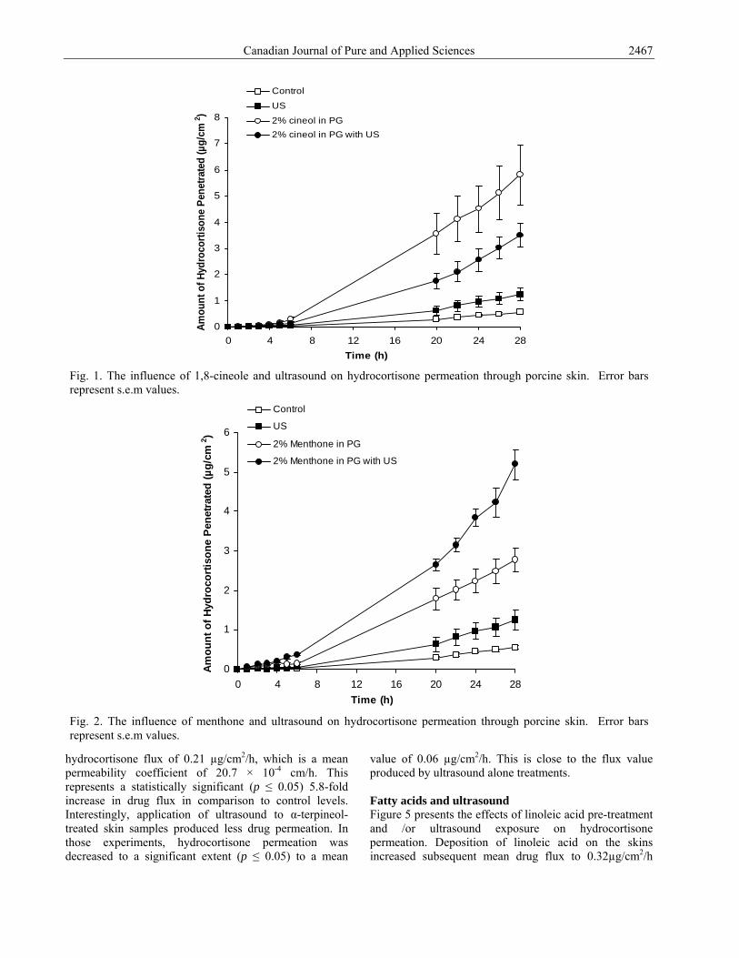
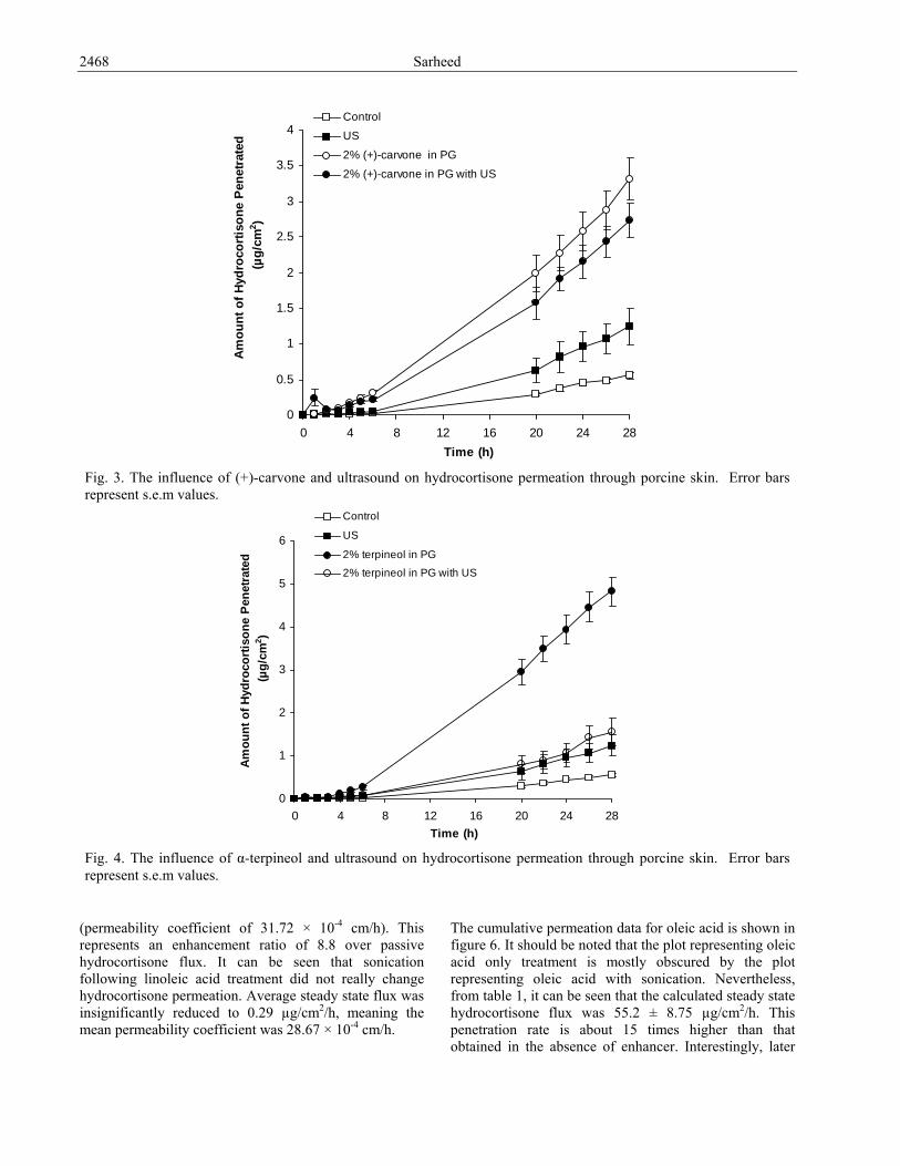
Terpenes and ultrasound Figure 1 shows the hydrocortisone permeation plots under the influence of 20 kHz ultrasound and 1,8-cineole - a cyclic ether terepene. When 1,8-cineole was applied to porcine skin in the absence of ultrasound, a subsequent mean drug flux of 0.24 µg/cm2/h was measured. This is equivalent to a permeability coefficient of 24.5 × 10⁻⁴ cm/h. This represented a significant enhancement (p ≤ 0.05) of about 6.8-fold relative to passive hydrocortisone flux. Figure 1 also shows the effect of combining ultrasonication with 1,8-cineole pre-treatment. Surprisingly, the combination treatment produced a lower mean flux of 0.14 µg/cm2/h. This is equivalent to a permeability coefficient of 14.63 × 10⁻⁴ cm/h. It represents a 4-fold increase in flux over control levels. The data for menthone is shown in figure 2, it can be seen that menthone only application produced an average steady state hydrocortisone flux of 0.11 µg/cm2/h. This means the average permeability coefficient was 11.78 × 10⁻⁴ cm/h. This is about 3.2-fold higher than the passive hydrocortisone delivery. Menthone combined with ultrasound caused a further significant increase in the permeation of hydrocortisone so that the mean steady state value was 0.26 µg/cm2/h. This is approximately 7.4 times the mean control value. From table 1, it can be seen that ER [Menthone + Ultrasound] (7.4) > ER [Menthone] (3.2) + ER[Ultrasound] (2.4), strongly suggesting that a
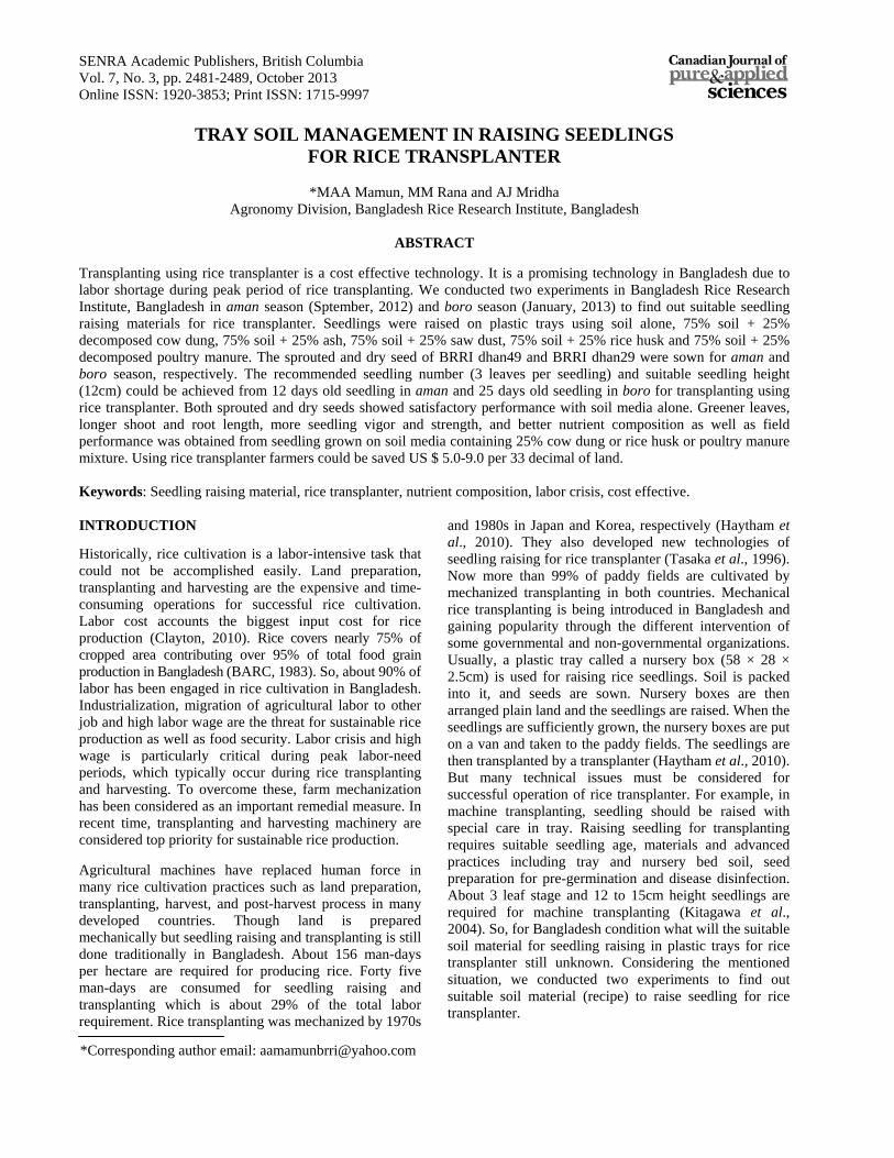
synergistic effect is occurring. However, this simple relationship just relates to the mean enhancement values. In order to be sure that synergism is developing and not just an additive effect, it is necessary to take into account the effect of the variability (error bars) of each measurement. This was done by performing a 2-way ANOVA. It was shown that there was indeed a significant interaction (p = 0.038) taking place between the ultrasound and the menthone. So synergism was occurring. Figure 3 depicts the effect of ultrasound and (+)-carvone pre-treatment on hydrocortisone permeation. Application of (+)-carvone alone caused a significant increase (p ≤ 0.05) in mean hydrocortisone flux (0.13 µg/cm2/h), representing an enhancement of 3.7-fold over average passive flux levels. Treatment with (+)-carvone followed by low frequency ultrasound caused a slight but statistically insignificant (p>0.05) decrease in hydrocortisone permeation compared to the effect of chemical enhancer alone. In this case, the mean flux was 0.11 µg/cm2/h and this can be converted to a permeability coefficient of 11.23 × 10⁻⁴ cm/h. This represents a 3.2-fold increase over mean passive flux. Figure 4 shows the influence of α-terpineol treatment on transdermal hydrocortisone penetration. Treatment of the skin samples with α-terpineol alone resulted in an average
Table 1. Steady state data for the chemical enhancer –ultrasound combination studies.
Treatment (replicates) Jss (µg cm-2 h-1) Mean ± s.e.m
kp × 10-4 (cm h-1)
Mean ± s.e.m E. R. #
Control (n=6) 0.03 ± 0.01 3.6 ± 0.75 1 US only (n=7) 0.08 ± 0.01 8.8 ± 1.34 2.4 1,8-cineole (n=7) 0.25 ± 0.04 24.5 ± 4.73 6.8 1,8-cineole + US (n=7) 0.15 ± 0.01 14.6 ± 1.94 4.1 Menthone (n=7) 0.12 ± 0.01 11.7 ± 1.31 3.2 Menthone + US (n=6) 0.27 ± 0.04 26.7 ± 4.24 7.4 (+)-carvone (n=7) 0.13 ± 0.01 13.2 ± 1.19 3.7 (+)-carvone + US (n=7) 0.11 ± 0.01 11.4 ± 1.02 3.2 α-Terpineol (n=7) 0.21 ± 0.01 20.7 ± 1.37 5.8 α-Terpineol + US (n=7) 0.06 ± 0.01 6.4 ± 1.30 1.8 Linoleic acid (n=7) 0.32 ± 0.06 31.7 ± 6.26 8.8 Linoleic acid + US (n=7) 0.29 ± 0.08 28.6 ± 8.43 7.9 Oleic acid (n=7) 0.55 ± 0.08 55.2 ± 8.75 15.3 Oleic acid + US (n=7) 0.51 ± 0.05 51.2 ± 5.81 14.2 Stearic acid + (n=7) 0.05 ± 0.01 5.09 ± 0.72 1.4 Stearic acid + US (n=7) 0.05 ± 0.01 4.57 ± 1.32 1.3 0.25% SLS (n=7) 0.19 ± 0.02 19.3 ± 2.75 5.4 0.25% SLS + US (n=7) 0.26 ± 0.02 25.9 ± 2.45 7.2 1% SLS (n=7) 0.15 ± 0.01 14.7 ± 1.83 4.1 1% SLS + US (n=7) 0.32 ± 0.07 31.6 ± 4.07 8.8
#Where E.R. represents the enhancement ratio relative to passive hydrocortisone flux in the absence of ultrasound or chemical treatment.
Canadian Journal of Pure and Applied Sciences 2467
hydrocortisone flux of 0.21 µg/cm2/h, which is a mean permeability coefficient of 20.7 × 10⁻⁴ cm/h. This represents a statistically significant (p ≤ 0.05) 5.8-fold increase in drug flux in comparison to control levels. Interestingly, application of ultrasound to α-terpineol-treated skin samples produced less drug permeation. In those experiments, hydrocortisone permeation was decreased to a significant extent (p ≤ 0.05) to a mean
value of 0.06 µg/cm2/h. This is close to the flux value produced by ultrasound alone treatments. Fatty acids and ultrasound Figure 5 presents the effects of linoleic acid pre-treatment and /or ultrasound exposure on hydrocortisone permeation. Deposition of linoleic acid on the skins increased subsequent mean drug flux to 0.32µg/cm2/h
0
1
2
3
4
5
6
7
8
0 4 8 12 16 20 24 28Time (h)
Amou
nt o
f Hyd
roco
rtiso
ne P
enet
rate
d (µ
g/cm
2 )
Control
US
2% cineol in PG2% cineol in PG with US
Fig. 1. The influence of 1,8-cineole and ultrasound on hydrocortisone permeation through porcine skin. Error barsrepresent s.e.m values.
0
1
2
3
4
5
6
0 4 8 12 16 20 24 28Time (h)
Am
ount
of H
ydro
cort
ison
e Pe
netra
ted
(µg/
cm2 )
Control
US
2% Menthone in PG
2% Menthone in PG with US
Fig. 2. The influence of menthone and ultrasound on hydrocortisone permeation through porcine skin. Error barsrepresent s.e.m values.
Sarheed 2468
(permeability coefficient of 31.72 × 10⁻⁴ cm/h). This represents an enhancement ratio of 8.8 over passive hydrocortisone flux. It can be seen that sonication following linoleic acid treatment did not really change hydrocortisone permeation. Average steady state flux was insignificantly reduced to 0.29 µg/cm2/h, meaning the mean permeability coefficient was 28.67 × 10⁻⁴ cm/h.
The cumulative permeation data for oleic acid is shown in figure 6. It should be noted that the plot representing oleic acid only treatment is mostly obscured by the plot representing oleic acid with sonication. Nevertheless, from table 1, it can be seen that the calculated steady state hydrocortisone flux was 55.2 ± 8.75 µg/cm2/h. This penetration rate is about 15 times higher than that obtained in the absence of enhancer. Interestingly, later
0
0.5
1
1.5
2
2.5
3
3.5
4
0 4 8 12 16 20 24 28Time (h)
Amou
nt o
f Hyd
roco
rtiso
ne P
enet
rate
d (µ
g/cm
2 )
Control
US
2% (+)-carvone in PG
2% (+)-carvone in PG with US
Fig. 3. The influence of (+)-carvone and ultrasound on hydrocortisone permeation through porcine skin. Error barsrepresent s.e.m values.
0
1
2
3
4
5
6
0 4 8 12 16 20 24 28Time (h)
Amou
nt o
f Hyd
roco
rtiso
ne P
enet
rate
d (µ
g/cm
2 )
Control
US
2% terpineol in PG
2% terpineol in PG with US
Fig. 4. The influence of α-terpineol and ultrasound on hydrocortisone permeation through porcine skin. Error barsrepresent s.e.m values.

Canadian Journal of Pure and Applied Sciences 2469
application of 20 kHz ultrasound did not significantly affect drug absorption in comparison to oleic acid only treatment. Figure 7 presents the plots for the stearic acid data. It is apparent that both the chemical enhancer only and chemical enhancer with sonication protocols produced
relatively mild drug transport enhancement of 1.4-fold and 1.3-fold, respectively. Sodium lauryl sulphate (SLS) and ultrasound Figure 8 depicts the hydrocortisone permeation data when 0.25% SLS was employed as the chemical enhancer. It can be seen that skin treatment with SLS only
0
1
2
3
4
5
6
7
8
9
10
0 4 8 12 16 20 24 28
Time (h)
Amou
nt o
f Hyd
roco
rtis
one
Pen
etrt
aed
(µg/
cm2 )
Control
US
2% linoleoc acid in PG
2% linoleic acid in PG with US
Fig. 5. The influence of linoleic acid and ultrasound on hydrocortisone permeation through porcine skin. Error barsrepresent s.e.m values.
0
3
6
9
12
15
0 4 8 12 16 20 24 28
Time (h)
Am
ount
of H
ydro
cort
ison
e P
enet
rate
d (µ
g/cm
2 )
ControlUS2% oleic acid in PG2% Oleic acid in PG with US
Fig. 6. The influence of oleic acid and ultrasound on hydrocortisone permeation through porcine skin. Error barsrepresent s.e.m values.

Sarheed 2470
significantly enhanced steady state hydrocortisone flux by over 5-fold relative to control levels. In fact, a mean flux of 0.19 µg/cm2/h was measured. When SLS-treated skin was exposed to 20 kHz ultrasound, drug flux was significantly enhanced even further to 0.26 ± 0.02 µg/cm2/h. By examining table 1, it can be shown that ER [0.25% SLS+ Ultrasound] (7.2) < ER [0.25% SLS] (5.4)
+ ER [Ultrasound] (2.4). This means that a synergistic effect could not be developing. Figure 9 presents the hydrocortisone permeation plots when a more concentrated 1% SLS solution was employed as the pre-treatment. Application of the surfactant solution significantly promoted drug flux over
0
0.2
0.4
0.6
0.8
1
1.2
1.4
1.6
0 4 8 12 16 20 24 28Time (h)
Amou
nt o
f Hyd
roco
rtiso
ne P
enet
rate
d (µ
g/cm
2 )
ControlUS2% stearic acid in EtOH2% stearic acid in EtOH with US
Fig. 7. The influence of stearic acid and ultrasound on hydrocortisone permeation through porcine skin. Error barsrepresent s.e.m values.
0
1
2
3
4
5
6
7
8
0 4 8 12 16 20 24 28
Time (h)
Amou
nt o
f Hyd
roco
rtiso
ne P
enet
rate
d (µ
g/cm
2 )
ControlUS0.25% SLS in PBS0.25% SLS in PBS with US
Fig. 8. The influence of 0.25% SLS and ultrasound on hydrocortisone permeation through porcine skin. Error barsrepresent s.e.m values.

Canadian Journal of Pure and Applied Sciences 2471
control levels to achieve a steady state value of 0.15 ± 0.01 µg/cm2/h. Later exposure of the skin sections to ultrasound resulted in a further significant increase of drug flux to 0.32 ± 0.07 µg/cm2/h. In terms of the mean enhancement ratios, it can be shown that: ER [1% SLS+ Ultrasound] (8.8) > ER [1% SLS] (4.1) + ER [Ultrasound] (2.4). This means a synergistic interaction between the surfactant treatment and ultrasound may have developed. A Two-way ANOVA indicated that there was indeed a significant interaction (p = 0.026) taking place between the ultrasound and the 1% SLS, providing evidence of synergism. DISCUSSION With regards to the terpenes, our results indicated that application of these chemicals in the absence of ultrasound produced significant enhancement of hydrocortisone delivery. The enhancement ratios produced in decreasing order of potency were: 1,8-cineole (6.8) > α-terpineol (5.8) > (+)-carvone (3.7) > menthone (3.2). This rank order is somewhat similar but not identical to that reported by others who measured hydrocortisone flux through hairless mouse skin in vitro (El-Kattan et al., 2000). That group reported an order of: menthone > 1,8-cineole > α-terpineol > (+)-carvone. The very different nature of the tested skins may explain the different ranking for menthone. Ultrasonication of skins following terpene application did not actually improve hydrocortisone permeation except where the terpene was
menthone. Here, we identified synergism causing a 7.4-fold increase in drug flux over control levels. For the tested fatty acids, our enhancement ratios for hydrocortisone permeation occurred in the following order: oleic acid (15.3) > linoleic acid (8.8) > stearic acid (1.4). This type of pattern in which oleic acid seems to be the optimal enhancer has been reported many times before in the literature, with perhaps the research of Kim et al. (2008) being the most recent example. The very low potency of stearic acid might be due to the fact that an ethanolic vehicle was used to dissolve this enhancer and it is known that ethanol can under certain circumstances reduce the permeation of some drugs (Fang et al., 2003). Interestingly, ultrasonication of each fatty acid-treated skin samples did not cause any further increase in hydrocortisone delivery. With respect to SLS, our findings indicated that the 0.25% concentration was marginally more permeabilising to the skin than the 1% concentration. It is unclear why this should be the case. More interesting was the fact that ultrasound exposure following 1% SLS treatment caused a highly significant synergistic 8.8-fold increase in hydrocortisone delivery. Treatment with 0.25% SLS and ultrasound caused a significant additive effect. CONCLUSION To summarize, the main finding of this work is that using the fatty acids or the terpenes (excepting menthone) in
0
2
4
6
8
10
0 4 8 12 16 20 24 28
Time (h)
Amou
nt o
f Hyd
roco
tison
e Pe
netra
ted
(µg/
cm2 )
ControlUS1% SLS in PBS1% SLS in PBS with US
Fig. 9. The influence of 1% SLS and ultrasound on hydrocortisone permeation through porcine skin. Error barsrepresent s.e.m values.

Sarheed 2472
combination with ultrasonication does not produce a synergistic or even additive flux enhancement effect. In contrast, use of SLS followed by ultrasound does yield additive or synergistic activities, depending upon the SLS concentration applied. A possible explanation for these differences is due to the lipid-protein partitioning (LPP) concept (Williams and Barry, 1991a; Williams and Barry, 1991b; Barry, 2006). This theory classifies chemical enhancers into three categories depending upon how they work. Terpenes and fatty acids fall into the first class of enhancers. These chemicals modify the structured intercellular lipid domains of the stratum corneum, making the stratum corneum more permeable. In contrast, ionic surfactants such as SLS fall into the second class of enhancers that act at stratum corneum desmosomes and protein structures (Barry, 2006). Considerable evidence suggests that low frequency ultrasound causes stratum corneum disordering of lipids that may be relatively similar to the changes provoked by terpenes and fatty acids. It may be that a combination of lipid domain and protein domain changes is required for synergism to take place. Finally, it should be mentioned that in our studies, skin samples were treated with chemical enhancers while the drug solution and ultrasound were applied later. This methodology has the advantage that it avoids complex three way interactions occurring between the drug, the enhancer and the ultrasound. However, a simultaneous administration of all three treatments could be more effective and probably simpler to apply in a clinical setting. ACKNOWLEDGMENTS The author is grateful to Dr. Victor Meidan and Prof. Gillian M. Eccleston for the academic support. DECLARATION OF INTERESTS The research was partially supported by the University of Strathclyde, Glasgow, UK. REFERENCES Aungst, BJ., Rogers, J. and Shefter, E. 1986. Enhancement of naloxone penetration through human skin in vitro using fatty acids, fatty alcohols, surfactants, sulfoxides and amides. Int. J. Pharm. 33:225-234.
Aungst, BJ. 1989. Structure/effect studies of fatty acid isomers as skin penetration enhancers and skin irritants. Pharm. Res. 6:244-247.
Aungst, BJ., Blake, JA. and Hussain, MA. 1990. Contributions of drug solubilization, partitioning, barrier disruption, and solvent permeation to the enhancement of
skin permeation of various compounds with fatty acids and amines. Pharm. Res. 7:712-718.
Asbill, CS. and Michniak, BB. 2000. Percutaneous penetration enhancers: local versus transdermal activity. Pharm. Sci. Technol. Today. 3:36-41.
Bhatia, KS. and Singh, J. 1998. Synergistic effect of iontophoresis and a series of fatty acids on LHRH permeability through porcine skin. J. Pharm. Sci. 87:462-469.
Barry, BW. 2006. Penetration enhancer classification. In: Percutaneous Penetration Enhancers. Eds. Smith, EW. and Maibach, HI. Taylor & Francis Group, New York, USA. 3-11.
Cornwell, PA. and Barry, BW. 1993. The routes of penetration of ions and 5-fluorouracil across human skin and the mechanisms of action of terpene skin penetration enhancers. Int. J. Pharm. 94:189-194.
Cotte, M., Dumas, P., Besnard, M., Tchoreloff, P. and Walter, P. 2004. Synchrotron FT-IR microscopic study of chemical enhancers in transdermal drug delivery: example of fatty acids. J. Control. Rel. 97:269-281.
Elyan, BM., Sidhom, MB. and Plakogiannis, FM. 1996. Evaluation of the effect of different fatty acids on the percutaneous absorption of metaproterenol sulfate. J. Pharm. Sci. 85:101-105.
El-Kattan, AF., Asbill, CS. and Michniak, BB. 2000. The effect of terpene enhancer lipophilicity on the percutaneous permeation of hydrocortisone formulated in HPMC gel systems. Int. J Pharm. 198:179-189.
El-Kattan AF., Asbill, CS., Kim, N. and Michniak, BB. 2001. The effects of terpene enhancers on the percutaneous permeation of drugs with different lipophilicities. Int. J. Pharm. 215:229-240.
Fuhrman, LC., Michniak, BB., Behl, CR. and Malick, AW. 1997. Effect of novel penetration enhancers on the transdermal delivery of hydrocortisone: an in vitro species comparison. J. Control. Rel. 45:199-206.
Fang, JY., Hwang, TL. and Leu, YL. 2003. Effect of enhancers and retarders on percutaneous absorption of flurbiprofen from hydrogels. Int. J. Pharm. 250:313-325.
Fang, JY., Tsai, TH., Lin, YY., Wong, WW., Wang, MN. and Huang, JF. 2007. Transdermal delivery of tea catechins and theophylline enhanced by terpenes: a mechanistic study. Biol. Pharm. Bull. 30:343-349.
Godwin, DA. and Michniak, BB. 1999. Influence of drug lipophilicity on terpenes as transdermal penetration enhancers. Drug Dev. Ind. Pharm. 25:905-915.
Hori, M., Satoh, S., Maibach, HI. and Guy, RH. 1991. Enhancement of propranolol hydrochloride and diazepam

Canadian Journal of Pure and Applied Sciences 2473
skin absorption in vitro: effect of enhancer lipophilicity. J. Pharm. Sci. 80:32-35.
Ho, HO., Chen, LC., Lin, HM. and Sheu, MT. 1998. Penetration enhancement by menthol combined with a solubilization effect in a mixed solvent system. J. Control. Rel. 51:301-311.
Kim, MJ., Doh, HJ., Choi, MK., Chung, SJ., Shim, CK., Kim, DD., Kim, JS., Yong, CS. and Choi, HG. 2008. Skin permeation enhancement of diclofenac by fatty acids. Drug Deliv. 15:373-379.
Mitragotri, S., Ray, D., Farrell, J., Tang, H., Yu, B., Kost J., Blankschtein, D. and Langer, R. 2000. Synergistic effect of low-frequency ultrasound and sodium lauryl sulfate on transdermal transport. J. Pharm. Sci. 89:892-900.
Mutalik, S., Parekh, HS., Davies, NM. and Udupa, N. 2009. A combined approach of chemical enhancers and sonophoresis for the transdermal delivery of tizanidine hydrochloride. Drug Deliv. 16:82-91.
Narishetty, ST. and Panchagnula, R. 2004. Transdermal delivery of zidovudine: effect of terpenes and their mechanism of action. J. Control. Rel. 95:367-379.
Nokhodchi, A., Sharabiani, K., Rashidi, MR. and Ghafourian, T. 2007. The effect of terpene concentrations on the skin penetration of diclofenac sodium. Int. J. Pharm. 335:97-105.
Okabe, H., Takayama, K., Ogura, A. and Nagai, T. 1989. Effect of limonene and related compounds on the percutaneous absorption of indomethacin. Drug. Des. Deliv. 4:313-321.
Rowat, AC., Kitson, N. and Thewalt, JL. 2006. Interactions of oleic acid and model stratum corneum membranes as seen by 2H NMR. Int. J. Pharm. 307:225-231.
Sarheed, O. and Frum, Y. 2012. Use of the skin sandwich technique to probe the role of the hair follicles in sonophoresis. Int. J. Pharm. 423:179-183.
Vaddi, HK., Ho, PC. and Chan, SY. 2002. Terpenes in propylene glycol as skin-penetration enhancers: permeation and partition of haloperidol, Fourier transform infrared spectroscopy, and differential scanning calorimetry. J. Pharm. Sci. 91:1639-1651.
Walters, KA. and Roberts, MS. 1993. Veterinary Applications of Skin Penetration Enhancers. In: Pharmaceutical Skin Penetration Enhancement. Eds. K.A. Walters, KA. and Hadgraft, J. Marcel Dekker, New York, USA. 345-364.
Wang, MY., Yang, YY. and Heng, PW. 2004. Role of solvent in interactions between fatty acids-based
formulations and lipids in porcine stratum corneum. J. Control. Rel. 94:207-216.
Williams, AC. and Barry, BW. 1991a. The enhancement index concept applied to penetration enhancers for human skin and model lipophilic (estradiol) and hydrophilic (5-fluorouracil) drugs. Int. J. Pharm. 74:157-168.
Williams, AC. and Barry, BW. 1991b. Terpenes and the lipid-protein-partitioning theory of skin penetration enhancement. Pharm. Res. 8:17-24.
Williams, AC. and Barry, BW. 2004. Penetration enhancers. Adv. Drug Deliv. Rev. 56:603-618.
Received: May 13, 2013; Accepted: July 2, 2013

SENRA Academic Publishers, British Columbia Vol. 7, No. 3, pp. 2475-2480, Oct 2013 Online ISSN: 1920-3853; Print ISSN: 1715-9997
POPULATION BIOLOGY OF A CESTODE, PROTEOCEPHALUS FILICOLLIS (RUDOLPHI) FROM GASTEROSTEUS ACULEATUS L. IN SCOTLAND
*Zafar Iqbal and Rod Wootten
Institute of Aquaculture, University of Stirling, FK9 4LA, Scotland, UK
ABSTRACT
Seasonal changes in the biology of Proteocephalus filicollis were investigated for 27 months in three-spined stickleback, Gasterosteus aculeatus from Airthrey Loch Scotland. A total of 1301 fishes were sampled and 1949 P. filicollis worms were extracted. Proteocephalus filicollis were abundant throughout the year as indicated by high prevalence (38.66%), mean intensity (3.87) and abundance (1.49). Monthly prevalence and abundance showed significant difference in two years. Growth and maturation of P. filicollis showed a marked seasonal cycle, as both of these were occurring in spring and summer. The monthly mean length of worm showed positive correlation with water temperature (Year I, r2=93.1; Year II, r2=77.9) but negative correlation with mean intensity (Year I, r2 =30.7; Year II, r2 =5.6). The recruitment of plerocercoid worms occur throughout the year. Four factors are proposed which influence the maturation of P. filicollis; rise in water temperature in summer, low mean intensity; host length and host endocrine system. The natural population of P. filicollis is generally high in Airthray Loch and is correlated to abiotic factors and eutrophic nature of the Loch. Keywords: Proteocephalus filicollis, cestode, three-spined stickleback, infection, recruitment, growth maturation. INTRODUCTION Seasonal cycle of maturation, growth and recruitment has commonly been observed in species of Proteocephalus (Kennedy, 1977). Proteocephalus filicollis is a cestode parasite of Gasterosteus aculeatus (Willemese, 1969). Hopkins (1959), Chappall (1969) and Iqbal (1998) studied some aspects of biology and seasonal cycle of this parasite from G. aculeatus. Proteocephalus filicollis has two host life cycles, the intermediate host is a cyclope copepod, Acanthocephalus robustus and the final host is G. aculeatus (Iqbal and Wootten, 2001). Proteocephalus filicollis worms are recruited in summer and autumn grow throughout the year and shed eggs in spring and summer (Iqbal and Wootten, 2008a, b). Some of the studies on biology of genus Proteocephalus are by; Fischer and Freeman (1969), Kennedy and Hine (1969), Willemse (1969), Wootten (1974), Eure (1976), Hanzelova et al. (1990), Pertierra and Nunez (1990), Nie and Kennedy (1991), Ieshko and Anikieva (1992), Iqbal, (1998), Wilson and Camp Jr (2003), Gilliland and Muzzall (2004) and Maillo et al. (2005). The studies by Willemse (1969), Chappall (1969), Dartnall (1972) and Rodland (1979) have given a much diversified picture of infection and biology of P. filicollis in G. aculeatus from different localities in Britain and Europe. Although, there is some conflict concerning the seasonality of other members of genus Proteocephalus, but most authors observed that in temperate water, worms mature and shed eggs in spring and early summer and recruitment starts in summer and
autumn. The aim of this study was to further look into the population biology of P. filicollis from a wild population of G. aculeatus and compare it with previous studies from Britain. MATERIALS AND METHODS The fish, G. aculeatus were collected with help of hand net on monthly basis (April 1993 to June 1995) from Airthrey Loch (situated within the grounds of University of Stirling, Scotland; Grid Reference 806965). Iqbal and Wootten (2004) have described the physicochemical and biological features of the Loch. The procedures of sampling, examination of fish and processing of parasites are given by Iqbal and Wootten (2005). Proteocephalus filicollis worms were identified according to Hopkins (1959). The worm samples are divided in to two populations as; Year I (July 1993- June 1994) and Year II (July 1994 to June 1995). The measurement of worms (total length) was taken from Mayer’s paracarmine stained and mounted specimens. Each worm was assigned to one of the five groups according to their maturity state. Plerocerciforms: newly recruited worms, Immature: worms which started segmentation, Maturing: worm with developing genital structure, Mature: worms with developed genital structure, Gravid: worms containing eggs. Prevalence, abundance and mean intensity was followed after Margolis et al. (1982). Pearson correlation was applied to see the relationship in prevalence, mean intensity and abundance; monthly mean length, water
*Corresponding author present address: Department of Zoology, University of the Punjab, Quaid-E-Azam Campus, Lahore, Pakistan Email: [email protected]

Iqbal and Wootten 2476
temperature and mean intensity of Protoecephalus filicollis. RESULTS A total of 1301 G. aculeatus were examined, of which 503 fishes were infected with P. filicollis. Altogether, 1976 worms were recovered from rectum and various sections of the intestine of the fish. The prevalence of P. filicollis was 38.66%, mean intensity 3.87 and abundance 1.49. The monthly prevalence fluctuated over study period, which rose from July (Year 1) to October then falling and rising through November to January and declining gradually from February to June. In the Year II, the same pattern of prevalence was observed i.e. rising from July to October then falling and rising through November to February and declining in March and rising from April to May and falling in June (Fig.1A). Mean intensity increased from July (Year 1) to November and dropped from December until June. In the Year II, mean intensity rose from July to December and dropped from February until June (Fig.1B). The mean intensity observed in Year I, followed the same pattern in the Year II. The rise and fall of mean intensity almost followed the same pattern as exhibited by prevalence in both years. There was a significant difference in the monthly prevalence and abundance of P. filicollis in Year I and Year II (T =-7.04, df. 545 P= 0.000; Mean intensity T = -7.04, df. 565, P=0.000). The seasonal prevalence and abundance of P. filicollis showed a clear pattern rising from summer (Year I) 23.4% through autumn (28.0%) to winter (36.4%) and then dropping from spring (31.0%) to summer (30.70%). The same pattern is observed in the Year II, prevalence and rising from autumn (56.6%) through winter (72.2%) and falling considerably from spring (62.2%) to summer (32.3%). Similarly, mean intensity showed the same pattern rising from summer (2.50) through autumn (3.76) to winter (3.17) and falling in spring (2.11). In Year II, mean intensity rose from summer (4.2) through autumn (4.41) to winter (5.36) and then falling in spring (4.58). The prevalence and mean intensity of P. filicollis was high in Year II generation (52.38%; 2.43) than in Year I generation (29.68%; 0.87). Plerocerciform worms (total length 0.32 to < 1.0mm) were found throughout the year. In April and May 1993 these worms comprised < 18%, and were 100% in July and August (Year I) but dropped to 88.75% in September. However, from October to April (Year I) the population of these worms was <14% and these worms were not present in May and June. In Year II, P. filicollis exhibited a different cycle of recruitment. The recruitment started in July and continued in September. Small plerocerciform worms (<16%) were present from October to June. Thus, in Year I recruitment of new generation of P. filicollis
occurred within two months of the loss of previous generation but in Year II there was some overlap of the two generations. The growth of P. filicollis starts just after the recruitment in summer and continue over autumn. In winter growth slows down or stops. However, from spring the growth starts again and is accelerated from April to June (Year I). A similar pattern occurred in Year II, although the increase in length was slow over winter and subsequent increase in length was rapid. Monthly mean length of P. filicollis was more in Year I than in Year II population (Fig. 2). The monthly mean length (ML) of P. filicollis (January to June 1994 and 1995 (Year I and II) showed positive regression with water temperature. The regression equation for Mean length vs. Temperature for year I was: ML= 1.51+ 0.69Temp; (P= 0.002); (r2=93.1) and for year II was: ML=0.96+0.58Temp; (P=0.020); (r2=77.9). However, monthly mean length of P. filicollis (January to June 1994 and 1995 (Year I and II) showed negative regression with mean intensity (MI). The regression equations for mean length vs. Mean intensity for year I was: ML = 14.25 - 2.86 MI; (r2 =30.7); (P= 0.254) and for year II; ML = 10.25 – 0.95 MI; (r2 =5.6); (P=0.651). Maturation of P. filicollis showed a marked seasonal pattern with bulk of population maturing in spring and early summer (Table 1). Occurrence of individual maturity stages of worm showed that immature (un-segmented) worms are present from July to May-June next year. Maturing (segmented) worms and mature worms (without eggs) were found from October to June. The maturing (segmented) worms comprise large population from April to June as compared to mature worms in the same period. Gravid worms were present from September to June in both years with some fluctuation in Year II. But these worms were always present from April to June. DISCUSSION This is another detailed investigation of population biology of P. filicollis in G. aculeatus. Prevalence of P. filicollis was high compared to earlier reports on this parasite. Low prevalence of P. filicollis i.e. 5% from G. aculeatus in Norway (Rodland, 1979) and high prevalence 40.2% in G. aculeatus in Netherlands (Willemse, 1969); 41% and 50% in G. aculeatus in Britain (Dartnall, 1972; Kenndy et al. (1992) has been observed. Mean intensity of P. filicollis was also high and it showed seasonal pattern of change. The high mean intensity in Year II generation may reflect high rate of recruitment. Population size of P. filicollis therefore, was high in this locality in G. aculeatus. The eutrophic nature of Airthray Loch and diversity of zooplankton in the loch (Iqbal and Wootten, 2004) may be suggested to increase

Canadian Journal of Pure and Applied Sciences 2477
the mean intensity. Moreover, the large population of infected copepod may have influenced the high transmission of P. filicollis in the final host. The high prevalence may be associated with warm late summer and autumn of Year I and Year II (Iqbal and Wootten, 2004). The high water temperature in Year I in Airthrey Loch may have operated by; 1) enhancing the feeding rate of G. aculeatus; 2) by favoring the establishment of worms in the fish; 3) providing higher biomass of zooplankton resulting in higher population of larval worms. The
parasite populations fluctuate on year to year basis as reported by Kennedy (1996) and the transmission rate of a parasite may be determined by the size of parasite population (Nie and Kennedy, 1991). The composition and abundance of suitable intermediate host in a locality may contribute to the distribution and infection level of a parasite. This view is supported by studies on Proteocephalus sp. indicating that more than one species of Cyclops may act as intermediate host in these cestodes (Wootten, 1974; Iqbal and Wootten, 2001).
Fig.1A
Fig. 1B
Fig.1. Monthly prevalence (1A) and mean intensity (1B) of Proteocephalus filicollis in Gasterosteus aculeatus fromAirthrey Loch, Scotland.

Iqbal and Wootten 2478
Proteocephalus filicollis showed continuous growth throughout the year. Increase in monthly mean length was greater in spring and summer but not in winter. Hopkins (1959) suggested that growth and development of P. filicollis is checked at low temperature from autumn to spring. The time of occurrence of gravid worms, reported in present study and is rather intermediate between two extremes reported by Hopkins (1959) and Chappall (1969). The majority of worm population became gravid in spring and summer. The reason for the discrepancy between results of present study and two earlier studies may be associated with difference in environmental conditions and habitat from where the fish was collected. It is clear that P. filicollis has definite period of maximum reproduction in spring and summer which coincide with rise in water temperature. The reproduction of P. filicollis exhibits seasonal pattern, with egg production taking place mainly in spring and summer. This type of reproductive cycle has adaptive significance for parasites requiring an intermediate host, as it ensures that most eggs are produced and released at the time of maximum copepod population, (when large number of susceptible copepod are available for infection). The P. filicollis eggs are larger in winter and spring and smaller in summer. Moreover, the number of eggs is positively correlated to length of gravid worm (Iqbal and Wootten, 2008a, b). Hence, P. filicollis was similar to other species in this genus (Kennedy and Hine, 1969; Fischer and Freeman, 1969; Wootten, 1974) as it showed basic seasonal pattern in egg production. The increase in water temperature in spring appears to be a major factor influencing growth and maturation of P. filicollis. Water temperature has been proposed as an
explanation for seasonal maturation of Proteocephalus sp. in their host (Kennedy, 1977). Variations in mean length of P. filicollis indicated that the parasite grow throughout the year. However, growth is accelerated in spring and summer. There is also fall in mean intensity of infection during this period. The low mean intensity of infection may also reduce competition within the parasite infrapopulation at a time when metabolic requirement of individual cestode associated with growth and eggs production is presumably increasing. Proteocephalus filicollis is expelled from G. aculeatus after egg production. Temperature related rejection appears to be a possible cause of parasite mortality. When water temperature rises most of the parasites are lost from the host. It is suggested that there may be four main factors, which influence the maturation of P. filicollis in G. aculeatus from Airthrey Loch; rise in water in spring and early summer, low mean intensity; host length and host endocrine system. The length range of various maturity stages of worms observed is comparable to previous studies (Hopkins, 1959; Chappell, 1969; Willemse, 1969). Recruitment of new generation of worms was at peak in summer. Recruitment has been reported to occur for various length of time during the year in different Proteocephalus species (Wootten, 1974; Eure, 1976; Nie and Kennedy, 1991; Ieshiko and Anikeva, 1992). The occurrence of gravid worms over autumn and winter months and the fact that these eggs are infective (Iqbal and Wootten, 2001) may indicate that some limited recruitment occur over this period. It is concluded that the population of P. filicollis was generally high in Airthrey Loch compared to earlier reports. The high prevalence of
Fig. 2 Monthly mean length (with standard deviation) of Proteocephalus filicollis from Gasterosteus aculeatus andmaximum water temperature of Airthrey Loch, Scotland.

Canadian Journal of Pure and Applied Sciences 2479
P. filicollis is correlated to abiotic factors and eutrophic nature of the Loch. ACKNOWLEDGEMENTS First author is grateful to Fisheries Department, Government of the Punjab for providing opportunity to complete this project. This study was funded by Asian Development Bank, Manila under “Second Pakistan Aquaculture Development Project, Punjab, Pakistan. We are thankful to University of the Punjab Lahore for providing funds for publication of this article. REFERENCES Chappall, LH. 1969. The parasites of the three-spined stickleback, Gasteroseus aculeatus L. from Yorkshire pond.1. Seasonal variations of parasites fauna. Journal of Fish Biology. 1:137-152.
Dartnall, HJG. 1972. Variations in the parasites fauna of the three-spined stickleback related to salinity and other
parameters. PhD. Thesis. University of London. UK. pp267.
Eure, H. 1976. Seasonal abundance of Proteocephalus ambloplitis (cestodea: Proteocephalidea) from largemouth bass living in heated reservoir. Parasitology. 73:205-212.
Fischer, H. and Freeman, RS. 1969. Penetration of parenteral plercercoid of Proteocephalus Ambloplitis (Leidy) into the gut of smallmouth bass. Journal of Parasitology. 55:766-774.
Gillilland, MG. and Muzzall, PM. 2004. Microhabitat Analysis of Bass Tapeworm, Proteocephalus ambloplitis (Eucestoda: Proteocephlidae) in smallmouth Bass, Micropterus dolomieu, and Largemouth Bass, Micropterus salmoides, from Gull Lake, Michigan, USA. Compar. Parasitology. 71(2):221-225.
Table 1. Maturity stages and mean length (mm) of Proteocephalus filicollis in Gasterosteus aculeatus.
Immature worm Maturing worms Mature worms Gravid worms Months % M.L S.D % M.L S.D % M.L S.D % M.L S.D
Apr. 93 36.3 2.6 ±1,85 18.9 3.2 ±0.52 25.9 5.0 ±0.95 18.9 11.6 ±2.39 May 18.2 2.1 ±0.77 - - - 31.8 9.2 ±1.72 5.0 10.6 ±4.66 Jun. 05.7 3.4 ±1.49 - - - 48.6 6.8 ±1.23 45.7 12.4 ±4.29 Jul. 100 0.6 ±0.10 - - - - - - - - - Aug 100 1.1 ±0.47 - - - - - - - - - Sept. 97.6 2.4 ±1.10 - - - - - - 2.4 4.0 - Oct. 90.0 2.7 ±0.89 1.3 2.4 - 2.6 5.0 - 5.1 8.2 ±4.79 Nov. 96.1 2.4 ±0.91 - - - - - - 3.9 6.2 ±0.06 Dec. 95.1 2.4 ±0.86 3.3 3.2 ±0.12 - - - 1.6 4.8 - Jan.94 81.5 3.3 ±1.28 1.9 3.7 - 9.2 4.0 ±0.17 7.4 6.0 ±1.12 Feb. 90 4.4 ±0.25 2.0 5.7 - 4.0 8.1 - 4.0 8.0 - Mar. 83.0 3.3 ±1.28 7.5 8.5 ±4.71 1.9 5.2 - 7.6 10.9 ±4.7 Apr. 70.3 3.6 ±1.60 18.9 5.4 ±1.33 2.7 7.8 ±460 8.1 9.3 ±2.7 May 17.1 3.9 ±1.70 14.3 6.2 ±0.76 5.7 11.4 ±4.60 62.9 13.8 ±5.38 Jun. - - - 20.0 6.2 ±0.76 5.0 13.8 - 75.0 15.5 ±8.06 Jul. 94.6 0.9 ±0.37 5.4 3.3 - - - - - - - Aug. 100 1.0 ±0.55 - - - - - - - - - Sept. 92.7 1.4 ±0.69 1.6 2.4 - - - - 5.7 5.0 ±1.59 Oct. 95.5 2.30 ±0.82 3.0 2.8 ±0.49 - - - 1.5 3.6 - Nov. 99.0 2.51 ±1.04 - - - - - - 1.0 4.0 - Dec. 96.5 2.60 ±0.90 3.5 3.9 ±1.25 - - - - - - Jan.95 95.4 2.59 ±1.28 2.3 3.2 - 2.3 9.8 - - - - Feb. 89.4 2.79 ±1.12 4.9 5.6 ±1.36 1.6 10.0 ±8.32 4.1 9.1 ±2.32 Mar. 77.3 2.69 ±1.12 10.7 4.3 ±1.34 2.7 7.9 ±0.93 9.3 8.6 ±0.85 Apr. 21.7 2.76 ±1.40 44.4 6.7 ±2.13 6.7 6.7 ±3.99 26.7 9.9 ±4.05 May 25.0 2.44 ±1.46 32.9 6.1 ±2.66 11.0 12.0 ±5.39 31.1 11.3 ±6.17 Jun. 15.3 1.91 ±1.05 2.8 8.0 ±2.92 16.7 12.7 ±1.70 65.2 15.0 ±4.56

Iqbal and Wootten 2480
Hanzelova, V., Zitnan, R. and Syseov, AV. 1990. The seasonal dynamics of invasion cycle of Proteocephalus neglectus (cestoda). Helmintology. 27:135-144.
Hopkins, CA. 1959. Seasonal variation in the incidence and development of the cestode Proteocephaus filicollis (Rud.1810) in Gasterosteus aculeatus (L.). Parasitology. 49:529-542.
Ieshko, EP. and Anikievva, LV. 1992. Life Table of the helminthes and their analysis with thecestode Proteocephalus percae (Cestoda, Proteocephalidae) a specific parasite of perch Perca fluviatilis taken as an example. Ecological Parasitology, 1:31-41.
Iqbal, Z. 1998. Aspects of the biology of the cestode, Proteocephalus filicollis (Rudolphi) from Gasterosteus aculeatus L. PhD. Thesis University of Stilring, Scotland, UK. pp288.
Iqbal, Z. and Wootton, R. 2001. Development of Proteocephalus filicollis, a cestode in the copepod intermediate host, under experimental conditions. Science International (Lahore). 13(1): 59-65.
Iqbal, Z. and Wootten, R. 2004. Biological and Physicochmical features of Airthrey Loch. Scotland, UK. Biologia (Pakistan). 50(2):175-182.
Iqbal, Z. and Wootten, R. 2005. Infection of Proteocephalus filicollis (Rudolphi) from Gasterosteus aculeatus L, three-spined stickleback, in relation to sex and length of host. Punjab University Journal of Zoology. 20(1):15-23.
Iqbal, Z. and Wootten, R. 2008a. Seasonal occurrence of Proteocephalus filicollis (Rudolphi) eggs in a Natural population of Gasterosteus aculeatus L. Biologia (Pakistan). 54(1):83-90.
Iqbal, Z. and Wootten. R. 2008b. Egg production and fecundity of Proteocephalus filicollis (Rudolphi) a cestode from a Gasterosteus aculeatus L. Biologia (Pakistan). 54 (2):147-154.
Kennedy, CR. 1977. The regulations of fish parasite population. In: Regulation of Parasite Population. Ed. Esch, GW. Academic Press, New York, USA. 63-109.
Kennedy, CR. 1996. Establishment, survival and site of selection of the cestode Eubothrium crassum in brown trout Salmo trutta. Parasitology. 112:347-355.
Kennedy, CR. and Hine, PM. 1969. Population Biology of the cestode Proteocephalus torulosus (Batsch) in dace Lecciscus leuciscus L. of the River Avon. Journal of Fish Biology. 1:209-219.
Kennedy, CR., Nie, P. and Rostron, J. 1992. An insect, Sialis lutaria, as a host for larval Proteocephalus sp. Journal of Helminthology. 66:7-16.
Maillo, PA.,Vich, MA., Salvado, H., Marques, A. and Gracia, PG. 2005. Parasites of Anguilla Anguilla (L.) from three costal lagoons of the River Ebro delta (West Mediterranean). Acta Parasitologica. 50(2):156-160.
Margolis, L., Esch, GW., Holmes, JC., Kuris, AM. and Schad, GA. 1981. The use of Ecological terms in Parasitology (Report of an Adhoc Committee of the American Society of Parasitologists). Journal of Parasitology. 68(1):131-132.
Nie, P. and Kennedy, CR. 1991. Population Biology of Proteocephalus macrolepis (Creplin) in European eel, Anguilla Anguilla (Linnaeus) in two small Rivers. Journal of Fish Biology. 38:921-927.
Pertierra, AA., Gil, DE. and Nuenz, MO. 1990. Seasonal dynamics and maturation of the cestode Proteocephalus jandia (Woodland, 1933) in catfish (Rhamdia sapo). Acta Parasitologica Polonica. 35:305-313.
Rodland, JT. 1979. Proteocephalus filicollis in Gasterosteus aculeatus. In: Proceedings of the 9th Symp. Scandin. Soci. Parasit. 15:33-34.
Willimese, JJ. 1969. The genus Poteocephalus in the Netherland. Journal of Helminthology.43:207-222.
Wilson, S. and Camp, JW. Jr. 2003. Helminths of Bluegills, Lepomis macrochirus, from a Northern Indiana pond. Comparative Parasitology. (70)1:88-92.
Wootten, R. 1974. Studies on the life history and development of Proteocephalus percae (Muller) (Cestoda: Proteocphalidae). Journal of Helminthology. 48:269-28.
Received: April 17, 2013; Accepted: July 6, 2013
SENRA Academic Publishers, British Columbia Vol. 7, No. 3, pp. 2481-2489, October 2013 Online ISSN: 1920-3853; Print ISSN: 1715-9997
TRAY SOIL MANAGEMENT IN RAISING SEEDLINGS FOR RICE TRANSPLANTER
*MAA Mamun, MM Rana and AJ Mridha
Agronomy Division, Bangladesh Rice Research Institute, Bangladesh
ABSTRACT
Transplanting using rice transplanter is a cost effective technology. It is a promising technology in Bangladesh due to labor shortage during peak period of rice transplanting. We conducted two experiments in Bangladesh Rice Research Institute, Bangladesh in aman season (Sptember, 2012) and boro season (January, 2013) to find out suitable seedling raising materials for rice transplanter. Seedlings were raised on plastic trays using soil alone, 75% soil + 25% decomposed cow dung, 75% soil + 25% ash, 75% soil + 25% saw dust, 75% soil + 25% rice husk and 75% soil + 25% decomposed poultry manure. The sprouted and dry seed of BRRI dhan49 and BRRI dhan29 were sown for aman and boro season, respectively. The recommended seedling number (3 leaves per seedling) and suitable seedling height (12cm) could be achieved from 12 days old seedling in aman and 25 days old seedling in boro for transplanting using rice transplanter. Both sprouted and dry seeds showed satisfactory performance with soil media alone. Greener leaves, longer shoot and root length, more seedling vigor and strength, and better nutrient composition as well as field performance was obtained from seedling grown on soil media containing 25% cow dung or rice husk or poultry manure mixture. Using rice transplanter farmers could be saved US $ 5.0-9.0 per 33 decimal of land. Keywords: Seedling raising material, rice transplanter, nutrient composition, labor crisis, cost effective. INTRODUCTION Historically, rice cultivation is a labor-intensive task that could not be accomplished easily. Land preparation, transplanting and harvesting are the expensive and time-consuming operations for successful rice cultivation. Labor cost accounts the biggest input cost for rice production (Clayton, 2010). Rice covers nearly 75% of cropped area contributing over 95% of total food grain production in Bangladesh (BARC, 1983). So, about 90% of labor has been engaged in rice cultivation in Bangladesh. Industrialization, migration of agricultural labor to other job and high labor wage are the threat for sustainable rice production as well as food security. Labor crisis and high wage is particularly critical during peak labor-need periods, which typically occur during rice transplanting and harvesting. To overcome these, farm mechanization has been considered as an important remedial measure. In recent time, transplanting and harvesting machinery are considered top priority for sustainable rice production. Agricultural machines have replaced human force in many rice cultivation practices such as land preparation, transplanting, harvest, and post-harvest process in many developed countries. Though land is prepared mechanically but seedling raising and transplanting is still done traditionally in Bangladesh. About 156 man-days per hectare are required for producing rice. Forty five man-days are consumed for seedling raising and transplanting which is about 29% of the total labor requirement. Rice transplanting was mechanized by 1970s
and 1980s in Japan and Korea, respectively (Haytham et al., 2010). They also developed new technologies of seedling raising for rice transplanter (Tasaka et al., 1996). Now more than 99% of paddy fields are cultivated by mechanized transplanting in both countries. Mechanical rice transplanting is being introduced in Bangladesh and gaining popularity through the different intervention of some governmental and non-governmental organizations. Usually, a plastic tray called a nursery box (58 × 28 × 2.5cm) is used for raising rice seedlings. Soil is packed into it, and seeds are sown. Nursery boxes are then arranged plain land and the seedlings are raised. When the seedlings are sufficiently grown, the nursery boxes are put on a van and taken to the paddy fields. The seedlings are then transplanted by a transplanter (Haytham et al., 2010). But many technical issues must be considered for successful operation of rice transplanter. For example, in machine transplanting, seedling should be raised with special care in tray. Raising seedling for transplanting requires suitable seedling age, materials and advanced practices including tray and nursery bed soil, seed preparation for pre-germination and disease disinfection. About 3 leaf stage and 12 to 15cm height seedlings are required for machine transplanting (Kitagawa et al., 2004). So, for Bangladesh condition what will the suitable soil material for seedling raising in plastic trays for rice transplanter still unknown. Considering the mentioned situation, we conducted two experiments to find out suitable soil material (recipe) to raise seedling for rice transplanter.
*Corresponding author email: [email protected]

Mamun et al. 2482
MATERIALS AND METHODS Plant and growth condition We conducted two experiments, first one in September (aman), 2012 and second one in January (boro), 2013 at the Bangladesh Rice Research Institute (BRRI), Gazipur, Bangladesh to find a suitable soil material for seedling raising for rice transplanter. The temperature of the two growing season was shown in figure 1. Boro season was relatively cooler than aman season. The seedlings were raised on plastic trays using 100% soil (T1), 75% soil + 25% decomposed cow dung (T2), 75% soil + 25% ash (T3), 75% soil + 25% saw dust (T4), 75% soil + 25% rice husk (T5) and 75% soil + 25% decomposed poultry manure (T6). The size of each tray was 58- x 28- x 2.5cm. The mixture of the material was sieved to remove the clods. The characteristics of soil were: pH 7.06, organic matter 1.07%, organic C 0.62%, N 0.046%, K 0.08 meq/100g, P 10.88 µg/g, S 11.45 µg/g and zinc 0.70 µg/g. The soil was sandy loam where the percentage of sand, silt and clay were 61.91, 33.33 and 4.76, respectively (Table 1). The nutrient status of cow dung, ash, saw dust, rice husk and poultry manure are presented in table 2. Initially the trays were placed in a plain field. Then one fourth of each tray was filled with clod free soil and organic materials. The sprouted and dry seed of BRRI dhan49 and BRRI dhan29 were sown for aman and boro season, respectively. The amount of seed was 130g (dry) and 150g (sprouted) per tray. Then the seeds were covered with clod free soil mixture and irrigate to keep moistened. The trays were irrigated 2 times every day. At the early stage of sowing we irrigate using knapsack sprayer. But after germination of seeds we use watering can to applied water to the trays. During rain in aman season and cold during boro season the trays were covered with polyethylene sheet. Seedlings of different soil media were analyzed for NPK uptake at the end of the nursery period (Jones, 1991). Samples were dried at 70°C for 24 hours and grinded to pass through a 20mm-mesh screen to estimate NPK uptake. A given amount of grinded samples were wet-digested with H2SO4, and potassium concentrations in the digested solution were determined using a flame spectrophotometer. The P concentration was determined by double beam spectrophotometer (Murphy and Riley, 1962). Total N was determined on composite plant samples by the Kjeldahl distillation method (Bremner, 1965). Measurement of seedling growth and dry matter production Seedlings were sampled from each tray. Twenty seedlings were selected randomly from each tray. The different growth parameters including leaf color, numbers, root and shoot length and dry weight, germination percent, seedling vigor and strength were taken. Leaf color was measured using leaf color chart. The were subjected to an ANOVA for the split plot design putting soil materials in
main plot and seed (sprouted vs. dry) in sub-plot by using MSTAT-C software (CIMMYT, Mexico City, Mexico) and the significance was tested by a variance ratio (i.e. F-value) at the 5% level (Gomez and Gomez, 1984). Field evaluation To evaluate the field performances we used walking type rice transplanter made by Republic of Korea, model: DP480. During transplanting we collected data on seedling number per hill, hills per m2, missing hill and area coverage by 4 tray seedlings. Cost evaluation Economic study and labour savings were calculated using Bangladeshi economic values. The cost for seed, labor for tray preparation and maintenance during seedling raising, seedling uprooting, carrying and transplanting were included for 33 decimal of land. The costs for seed = US$ 0.44 per kg, labor = US$ 3.75 per man day, hiring a tractor = US$ 2.5 per 33 decimals of land. The currency conversion factor used was 1 US$ = 80 Bangladeshi Taka.
0
5
10
15
20
25
30
35
1 2 3 4 5 6 7 8 9 10 11 12 13 14 15 16 17 18 19 20 21 22 23 24 25 26 27 28 29 30
Dates of month
Dai
ly m
ean
tem
pera
ture
(0 C)
September, 2012 January, 2013
Fig. 1. Temperature data of growing season.
Table 1. Physical and chemical properties of soil. Soil characters Unit Amount pH 7.06 Organic matter % 1.07 N % 0.046 P µg/g 10.88 K meq/100g 0.08 S µg/g 11.45 Sand % 61.91 Silt % 33.33 Clay % 4.76 Textural class Sandy loam
Table 2. Nutrient composition of organic materials used.
Materials MC (%) %N % P % K Cow dung 33 1.1 0.9 1.3 Ash 20 - - 2.0 Saw dust 30 0.4 0.3 1.1 Rice husk 27 0.6 0.4 1.3 Poultry manure 54 1.7 0.4 0.06

Canadian Journal of Pure and Applied Sciences 2483
RESULTS AND DISCUSSION Leaf color In aman season, soil management options exerted significant effect on leaf color (Table 3). Seed and interaction effect was not statistically significant. Greener leaf was obtained when soil was mixed with poultry manure followed by rice husk (Fig. 2: a-1). The leaf color was satisfactorily green when we used soil alone as well as mixture of soil with cow dung, saw dust in both type of seed. We found relatively yellow colored leaf using mixture of soil and ash. It might be because of ash contain no N which is responsible for greenness of plant leaf. During boro season, soil management options exerted significant effect on leaf color (Table 3). Seed and interaction effect was not statistically significant. Relatively greener leaf was observed when soil was mixed with rice husk followed by cow dung (Fig. 2: b-1). Slight leaf yellowing occurred in the trays of saw dust and poultry manure. Relatively yellow leaves were observed on trays where soil alone and ash mixture were used. The starting month of Boro season (December-January) is the coolest period in Bangladesh. Seedling damage is a common scenario in boro because of cold. But rice husk may act as an insulator or mulch to preserve soil temperature. Leaf number In aman season, soil management options exerted significant effect on leaf number (Table 3). Seed and
interaction effect was not statistically significant. The highest leaf number was calculated for sprouted and dry seed with the mixture of saw dust and poultry manure, respectively (Fig. 2: a-2). The leaf number was more than 2 per plant with soil alone and mixture of organic matter. During boro season, soil management options exerted significant effect on leaf number (Table 3). Seed and interaction effect was not statistically significant. The highest number of laves were recorded from sprouted and dry seed with soil alone and mixture of poultry manure, respectively. More than 2 leaves per plant were recorded from all cases of organic matter mixture (Fig. 2: b-2). Shoot length In aman seasons, shoot length influenced significantly due to individual effect of soil management options and seed. Interaction effect of two factors was not statistically significant (Table 3). The tallest seedling was obtained from soil mixture with poultry manure (Fig. 3: a-3). Sprouted seeds produced tallest seedling in all soil mixture. About 12.66 and 12 cm seedling were obtained from sprouted and dry seed, respectively. More than 11cm tall seedling was obtained from soil alone, mixture of cow dung, saw dust and rice husk. We recorded the shortest seedling with ash mixture. In boro season, soil management options exerted significant effect on shoot length (Table 3). Seed and interaction effect was not significant. The tallest seedling was obtained from soil mixture with poultry manure. The tallest seedling was obtained from the mixture of rice husk followed by
0
1
2
3
4
5
T1 T2 T3 T4 T5 T6
a-1
Leaf
col
or c
hart
valu
e Sprouted seed Dry seed
0
1
2
3
4
T1 T2 T3 T4 T5 T6
b-1
Leaf
col
or c
hart
valu
e Sprouted seed Dry seed
0
0.5
1
1.5
2
2.5
3
T1 T2 T3 T4 T5 T6
a-2
Leaf
num
ber
Sprouted seed Dry seed
0
0.5
1
1.5
2
2.5
3
T1 T2 T3 T4 T5 T6
b-2
Leaf
num
ber
Sprouted seed Dry seed
Soil management practices Soil management practices
Fig. 2. Leaf color and number as affected by seed and soil management practice, a = Aman and b = Boro season, T1 = 100% soil, T2 = 75% soil + 25% decomposed cow dung, T3 = 75% soil + 25% ash, T4 = 75% soil + 25% saw dust, T5 = 75% soil + 25% rice husk and T6 = 75% soil + 25% decomposed poultry manure.

Mamun et al. 2484
poultry manure and cow dung (Fig. 3: b-3). The length of tallest seedling was more than 13cm where above 12cm for second highest. The ash mixture produced the shortest seedling. Root length Seed exerted significant effect of seedling root length. The individual effect try management options and interaction of two factors did not show statistically significant effect on root length (Table 3). The longest root was recorded from sprouted and dry seed by for soil mixture of cow dung and soil alone, respectively (Fig. 3: a-4). Dry seeds produced longer root length than sprouted seeds. Sprouted seeds produced longest root length with the mixture of cow dung. Soil and other soil mixture produce similar root length. More than 4cm root length was calculated with soil alone and about 4cm was recorded from mixture of saw dust for dry seeds. Similar root length was recorded from the mixture of ash and poultry manure. Effect of soil management options and interaction of seed and soil management options was statistically significant during boro season for root length (Table 3). The individual effect of seed was not significant for root length. More or less similar root length was calculated from sprouted and dry seeds (Fig. 3: b-4). Above 6cm root was obtained from the mixture of rice husk. Soil mixture with ash or saw dust or poultry manure gave more than 5cm root. Soil alone and cow dung mixture produce lowest root length.
Dry matter production In aman seasons, dry matter production influenced by seed but individual effect of soil management practice and interaction was not statistically significant (Table 3). Sprouted seeds produced more dry matter than dry seeds per 20 seedlings in all cases of soil management practice (Fig. 4: a-5). In sprouted seed, the highest dry matter (426 mg) was recorded from saw dust mixture followed by soil alone. Soil mixed with poultry manure or cow dung or ash or rice husk produced similar dry matter in case of sprouted seed. Dry seed produced maximum dry matter (365mg) when seedlings are grown on soil mixed with poultry manure followed by rice husk and saw dust. Soil alone and cow dung mixture produced similar dry matter per 20 seedlings. Dry matter production influenced significantly due to individual effect of soil management and seed as well as interaction effect of two factors (Table 3) in boro season. Sprouted seeds gave maximum dry matter per 20 seedlings when grown on mixture of saw dust and it was 424 mg followed by poultry manure mixture (326 mg). Soil alone or mixture with cow dung or saw dust or ash produce similar amount of dry matter per 20 seedlings for sprouted seeds (Fig. 4: b-5). Dry seeds gave highest amount of dry matter (312mg per 20 seedlings) with cow dung mixture followed by rice husk mixture (291mg per 20 seedlings). The rest soil media produce similar amount of dry matter per 20 seedlings. The shoot dry weight mainly depends on the concentration of nutrients in the media, and the physical,
0
3
6
9
12
15
T1 T2 T3 T4 T5 T6
a-3
Shho
ot le
ngth
(cm
)
Sprouted seed Dry seed
0
3
6
9
12
15
T1 T2 T3 T4 T5 T6
b-3
Shho
ot le
ngth
(cm
)
Sprouted seed Dry seed
0
1
2
3
4
5
T1 T2 T3 T4 T5 T6
a-4
Roo
t len
gth
(cm
)
Sprouted seed Dry seed
01234567
T1 T2 T3 T4 T5 T6
b-4
Roo
t len
gth
(cm
)
Sprouted seed Dry seed
Soil management practice Soil management practice Fig. 3. Shoot and root length as affected by seed and soil management practice a = Aman and b = Boro season, T1 = 100% soil, T2 = 75% soil + 25% decomposed cow dung, T3 = 75% soil + 25% ash, T4 = 75% soil + 25% saw dust, T5 = 75% soil + 25% rice husk and T6 = 75% soil + 25% decomposed poultry manure.

Canadian Journal of Pure and Applied Sciences 2485
chemical and microbiological conditions for root activity and formation of new roots. In natural vegetation the shoot dry weight decreases as soil fertility decreases (Marschner, 1995). Seedling vigor In aman season, seedling vigor influenced significantly due to individual effect of soil management practice. Seed and interaction effect of two factors was not statistically significant (Table 3). More or less similar seedling vigor index was obtained for sprouted and dry seeds. In case of sprouted seed, the highest vigor index was found from the mixture of poultry manure (13.65) followed by cow dung or rice husk mixture (13). Seedling vigor was more or less similar for soil alone or mixture of saw dust and the value was above 12 (Fig. 4: a-6). In case of dry seeds, the highest vigor index was calculated for soil mixture with
poultry manure and it was above 13. The second highest vigor was calculated for seedling raising on soil mixture with saw dust followed by soil alone or rice husk. The lowest vigor index of rice seedling was calculated for soil with ash or cow dung. In boro season, seedling vigor influenced significantly due to individual effect of soil management practice. Seed and interaction effect of two factors was not statistically significant (Table 3). In sprouted seeds, the highest seedling vigor was obtained from seedlings produced on soil mixture with rice husk (>16) followed by saw dust and poultry manure (15). More or less similar vigor index was obtained from soil alone or soil mixture with cow dung or ash (Fig. 4: b-6). Seedling strength In aman season, seeds exerted significant influence on seedling strength (Table 3) but soil management options
0
100
200
300
400
500
T1 T2 T3 T4 T5 T6
a-5
Dry
wt.
of 2
0 se
edlin
g (m
g)
Sprouted seed Dry seed
0
100
200
300
400
500
T1 T2 T3 T4 T5 T6
b-5D
ry w
t. of
20
seed
ling
(mg)
Sprouted seed Dry seed
0
3
6
9
12
15
18
T1 T2 T3 T4 T5 T6
a-6
See
dlin
g vi
gor i
ndex
Sprouted seed Dry seed
0
3
6
9
12
15
18
T1 T2 T3 T4 T5 T6
b-6
See
dlin
g vi
gor i
ndex
Sprouted seed Dry seed
0.0
0.4
0.8
1.2
1.6
2.0
T1 T2 T3 T4 T5 T6
a-7
See
dlin
g st
reng
th (m
g cm
-1)
Sprouted seed Dry seed
0.0
0.4
0.8
1.2
1.6
2.0
T1 T2 T3 T4 T5 T6
b-7
See
dlin
g st
reng
th (m
g cm
-1)
Sprouted seed Dry seed
Soil management practice Soil management practice
Fig. 4. Dry matter production, seedling vigor and strength as affected by seed and soil management practice, a = Aman and b = Boro season, T1 = 100% soil, T2 = 75% soil + 25% decomposed cow dung, T3 = 75% soil + 25% ash, T4 = 75% soil + 25% saw dust, T5 = 75% soil + 25% rice husk and T6 = 75% soil + 25% decomposed poultry manure.

Mamun et al. 2486
and interaction effect was not statistically significant. The sprouted seeds produced seedlings with more strength than dry seeds. The seedling strength was highest when seedlings were grown on soil mixture with saw dust followed by soil alone (Fig. 4: a-7). More or less similar seedling strength was obtained from seedlings produced on soil mixture with cow dung or ash or saw dust or rice husk. Seedling strength was maximum when they were grown on soil mixture with poultry manure which statistically similar with seedling strength when they were grown on ash or saw dust or rice husk. The lowest seedling strength was found from seedling grown on soil alone and cow dung. In boro season, individual effect of soil management options and seed was not significant for seedling strength (Table 3) while interaction effect was significant. Sprouted seeds gave seedling with highest strength when
grown on soil with rice husk followed by poultry manure (Figure 4: b-7). Other treatments gave similar seedling strength. Dry seeds gave maximum seedling strength with cow dung mixture followed by saw dust and soil alone. The minimum seedling strength was obtained from poultry manure followed by seedling grown on soil alone or rice husk. Seedlings grown in the soil with cow dung or rice husk or poultry media displayed better seedling quality in terms of seedling vigor and its characteristics and suitability for rice mechanical transplanting. This result is similar to that observed by Wang et al. (1999). Nutrient composition of seedlings For sprouted seeds, nitrogen content was high on seedlings were grown on soil mixed with poultry manure followed by cow dung during aman season (Table 4). Seedlings from sprouted seeds contain higher amount K
Table 3. ANOVA results of different seedling parameters.
Sources of variations Leaf color chart value
Leaf number
Shoot length (cm)
Root length (cm)
Dry wt. of 20 seedling
(mg)
Seedling vigor index
Seedling strength
(mg cm-1) Aman, 2012 Soil management ** * ** NS NS ** NS Seed NS NS ** * ** NS ** Soil management x Seed NS NS NS NS NS NS NS Boro, 2013 Soil management ** * ** ** ** ** NS Seed NS NS NS NS * NS NS Soil management x Seed NS NS NS * ** NS *
* and ** indicate significant differences at P<0.05, P<0.01, respectively, and NS indicate not significant differences at the P<0.05 level. Table 4. Nutrient composition of seedlings.
Aman, 2012 Sprouted seeds Dry seeds
Age of seedling (days)
N (%) P (µg/g) K (meq/100g) N (%) P (µg/g) K (meq/100g) T1 0.28 1.61 2.78 0.30 1.72 2.88 T2 0.40 2.71 3.02 0.38 1.82 3.05 T3 0.29 1.78 3.11 0.34 1.45 3.16 T4 0.35 1.75 3.10 0.32 1.62 3.00 T5 0.36 1.92 3.00 0.37 1.73 3.02 T6 0.43 2.10 2.88 0.42 1.75 2.89
Boro, 2013 Sprouted seeds Dry seeds T1 0.24 1.67 2.67 0.28 1.20 2.64 T2 0.31 1.88 3.12 0.43 1.87 3.15 T3 0.23 1.34 3.24 0.34 1.45 3.30 T4 0.35 1.40 3.03 0.33 1.51 3.07 T5 0.34 1.43 3.12 0.38 1.56 3.14 T6 0.37 1.50 2.87 0.44 1.67 2.15
T1 = 100% soil, T2 = 75% soil + 25% decomposed cow dung, T3 = 75% soil + 25% ash, T4 = 75% soil + 25% saw dust, T5 = 75% soil + 25% rice husk and T6 = 75% soil + 25% decomposed poultry manure.

Canadian Journal of Pure and Applied Sciences 2487
and P when grown on cow dung or saw dust mixture. Nitrogen content was more in seedlings grown on poultry manure mixture followed by cow dung or rice husk mixture media. In boro season, seedling grown on media of poultry manure or saw dust or rice husk mixture contained higher amount of N for sprouted and dry seeds (Table 4). The amount of P was high for media containing cow dung or poultry manure. The amount of K was higher
for ash containing media. The organic matter based substrate had a notable N availability, which would cause a consistent N–P synergism on P uptake. The positive effect of organic matter based media on P uptake was evident. On the other hand, increases of P uptake in plants in response to N supply have also been reported in the literature (Matsushima, 1980). The growth traits may be attributed to the presence of amino acids and important
Table 5. Field performance of different seedling during transplanting by machine.
Aman, 2012 Sprouted seed Dry seed
Age of seedling (days) Seedlings
(hill-1) Hills (m-2)
Missing or floating
hills (m-2)
Area covered by 4 trays (m2)
Seedlings (hill-1)
Hills (m-2)
Missing or floating
hills (m-2)
Area covered by 4 trays (m2)
T1 7 24 2 200 7 22 1 208 T2 7 25 1 202 7 24 2 210 T3 8 23 2 200 8 24 2 199 T4 6 24 2 205 7 23 2 205 T5 6 23 2 198 7 24 2 198 T6 7 25 2 199 6 24 1 200
Boro, 2013 Sprouted seed Dry seed
T1 6 24 2 205 7 25 4 210 T2 6 23 1 202 8 24 2 208 T3 7 24 3 198 6 23 3 196 T4 5 25 2 200 6 23 2 205 T5 9 24 2 200 8 24 1 200 T6 5 25 2 200 9 23 2 196
T1 = 100% soil, T2 = 75% soil + 25% decomposed cow dung, T3 = 75% soil + 25% ash, T4 = 75% soil + 25% saw dust, T5 = 75% soil + 25% rice husk and T6 = 75% soil + 25% decomposed poultry manure. Table 6. Economic analysis of transplanting by rice transplanter vs. hand transplanting for 33 decimal of land.
Rice transplanter Hand transplanting Cost Cost S.
No. Heads Tk. US$ Heads Tk. US$ 1. Seed (140g/tray) for 27
trays 125.00 1.57 Labor for seed and seed bed
preparation - 1 man-days 300.00 3.75
3. Labor requirements for tray preparation, seed sowing, watering and maintenance
Seed 175.00 2.19
a. Aman (15 days) - 2 man-days
600.00 7.50 Labor for seedbed maintenance - 1 man-days
300.00 3.75
b. Boro (30 days) - 2 man-days
900.00 11.25 Labor for seedling uprooting and transplanting - 4 man-days
1200.00 15
4. Labor for seedling carrying and transplanting
300.00 3.75
5. Fuel for transplanting 200.00 2.5 6. Total cost Aman season 1225.00 15.32 Boro season 1525.00 19.07 1975.00 24.69
Labor: 300.00 Tk./man day, Seed: 35 Tk./Kg, Fuel: 100 Tk./lit. 1 $ = 80.00 Tk.
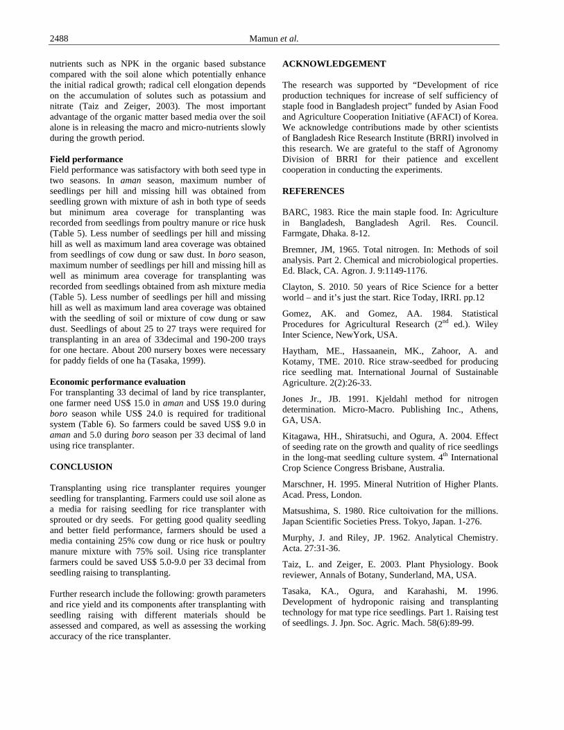
Mamun et al. 2488
nutrients such as NPK in the organic based substance compared with the soil alone which potentially enhance the initial radical growth; radical cell elongation depends on the accumulation of solutes such as potassium and nitrate (Taiz and Zeiger, 2003). The most important advantage of the organic matter based media over the soil alone is in releasing the macro and micro-nutrients slowly during the growth period. Field performance Field performance was satisfactory with both seed type in two seasons. In aman season, maximum number of seedlings per hill and missing hill was obtained from seedling grown with mixture of ash in both type of seeds but minimum area coverage for transplanting was recorded from seedlings from poultry manure or rice husk (Table 5). Less number of seedlings per hill and missing hill as well as maximum land area coverage was obtained from seedlings of cow dung or saw dust. In boro season, maximum number of seedlings per hill and missing hill as well as minimum area coverage for transplanting was recorded from seedlings obtained from ash mixture media (Table 5). Less number of seedlings per hill and missing hill as well as maximum land area coverage was obtained with the seedling of soil or mixture of cow dung or saw dust. Seedlings of about 25 to 27 trays were required for transplanting in an area of 33decimal and 190-200 trays for one hectare. About 200 nursery boxes were necessary for paddy fields of one ha (Tasaka, 1999). Economic performance evaluation For transplanting 33 decimal of land by rice transplanter, one farmer need US$ 15.0 in aman and US$ 19.0 during boro season while US$ 24.0 is required for traditional system (Table 6). So farmers could be saved US$ 9.0 in aman and 5.0 during boro season per 33 decimal of land using rice transplanter. CONCLUSION Transplanting using rice transplanter requires younger seedling for transplanting. Farmers could use soil alone as a media for raising seedling for rice transplanter with sprouted or dry seeds. For getting good quality seedling and better field performance, farmers should be used a media containing 25% cow dung or rice husk or poultry manure mixture with 75% soil. Using rice transplanter farmers could be saved US$ 5.0-9.0 per 33 decimal from seedling raising to transplanting. Further research include the following: growth parameters and rice yield and its components after transplanting with seedling raising with different materials should be assessed and compared, as well as assessing the working accuracy of the rice transplanter.
ACKNOWLEDGEMENT The research was supported by “Development of rice production techniques for increase of self sufficiency of staple food in Bangladesh project” funded by Asian Food and Agriculture Cooperation Initiative (AFACI) of Korea. We acknowledge contributions made by other scientists of Bangladesh Rice Research Institute (BRRI) involved in this research. We are grateful to the staff of Agronomy Division of BRRI for their patience and excellent cooperation in conducting the experiments. REFERENCES BARC, 1983. Rice the main staple food. In: Agriculture in Bangladesh, Bangladesh Agril. Res. Council. Farmgate, Dhaka. 8-12.
Bremner, JM, 1965. Total nitrogen. In: Methods of soil analysis. Part 2. Chemical and microbiological properties. Ed. Black, CA. Agron. J. 9:1149-1176.
Clayton, S. 2010. 50 years of Rice Science for a better world – and it’s just the start. Rice Today, IRRI. pp.12
Gomez, AK. and Gomez, AA. 1984. Statistical Procedures for Agricultural Research (2nd ed.). Wiley Inter Science, NewYork, USA.
Haytham, ME., Hassaanein, MK., Zahoor, A. and Kotamy, TME. 2010. Rice straw-seedbed for producing rice seedling mat. International Journal of Sustainable Agriculture. 2(2):26-33.
Jones Jr., JB. 1991. Kjeldahl method for nitrogen determination. Micro-Macro. Publishing Inc., Athens, GA, USA.
Kitagawa, HH., Shiratsuchi, and Ogura, A. 2004. Effect of seeding rate on the growth and quality of rice seedlings in the long-mat seedling culture system. 4th International Crop Science Congress Brisbane, Australia.
Marschner, H. 1995. Mineral Nutrition of Higher Plants. Acad. Press, London.
Matsushima, S. 1980. Rice cultoivation for the millions. Japan Scientific Societies Press. Tokyo, Japan. 1-276.
Murphy, J. and Riley, JP. 1962. Analytical Chemistry. Acta. 27:31-36.
Taiz, L. and Zeiger, E. 2003. Plant Physiology. Book reviewer, Annals of Botany, Sunderland, MA, USA.
Tasaka, KA., Ogura, and Karahashi, M. 1996. Development of hydroponic raising and transplanting technology for mat type rice seedlings. Part 1. Raising test of seedlings. J. Jpn. Soc. Agric. Mach. 58(6):89-99.

Canadian Journal of Pure and Applied Sciences 2489
Tasaka, K. 1999. Raising and Transplanting Technology for Long Mat with Hydroponically Grown Rice Seedlings. JARQ. 33:31-37.
Wang, DL., J. Zhu, Li, ZK. and Paterson, AH. 1999. Mapping QTLs with epistatic effects and QTL environment interactions by mixed linear model approaches. Theor. Appl. Genet. 99:1255-1264.
Received: June 13, 2013; Accepted: July 2, 2013

SENRA Academic Publishers, British Columbia Vol. 7, No. 3, pp. 2491-2498, October 2013 Online ISSN: 1920-3853; Print ISSN: 1715-9997
PHYTOCHEMICAL AND BIOLOGICAL EVALUATION OF POLYGONUM AMPLEXICAULE RHIZOME EXTRACT
*Muhammad Sheeraz Ahmad1, S M Saqlan Naqvi1, Sajida Mushtaq1,
Farzana Ramzan1, Abdul Sami1, Salma Batool1, Ihsan-ul-Haq2 and Bushra Mirza3 1Department of Biochemistry, PMAS Arid Agriculture University Rawalpindi
2Department of Pharmacy and 3Department of Biochemistry, Quiad-i-Azam University, Islamabad, Pakistan
ABSTRACT Medicinal plants have long been recognized for their applications in pharmaceutical, cosmetic, agriculture and food industry. The medicinal plants of genus Polygonum have far been used for a variety of purposes including the treatment of infectious diseases, inflammatory conditions, gastrointestinal disorders and cancer. Polygonum amplexicaule has folk medicinal use in Pakistan for such diseases. Since, the discovery of therapeutic agents depends on the knowledge of chemical constituents of the plant hence the present study was designed to evaluate the phytochemicals present in this specie’s rhizome with respect to their importance in the field of phytomedicines. Different phytochemicals were analyzed qualitatively by using various assays. Antitumor and brine shrimp cytoxicity assay were performed along with tyrosinase inhibition assay to check the suitability of the extract for cosmetics. The qualitative analysis of phytochemicals reveals the presence of various secondary metabolites that includes alkaloids, steroids, cardiac glycosides, saponins, fixed oils and fats, phenolic compounds including flavonoids, saponins, tannins and terpenoids, gums and mucilages and anthraquinones, while phytosterols and phlabatannins have not been detected. The rhizome extract has shown significant cytotoxic and antitumor activities with 13.57µg/mL IC50 towards brine shrimp assay. The tyrosinase inhibition assay validates its suitability for cosmetics with 64.6% tyrosinase inhibition at 10µg/ml treatment. The phytochemicals evaluated in the rhizome extract of P. amplexicaule and its biological activities validates its folkloric use and prospects its future use towards isolation of therapeutic agents. Keywords: Phytochemicals, biological screening, P. amplexicaule, Rhizome extract. INTRODUCTION Plants are very expedient and self-generating machines, producing a range of active poisonous and medicinal compounds. These active constituents are actually plant secondary metabolites and a particular combination of such metabolites may be taxonomically distinct attributing uniqueness of medicinal actions to particular plant species or even higher taxa (Ahmad et al., 2011; Parekh et al., 2007, 2006). These natural products can be obtained from any part of the plant i.e., roots, rhizomes, shoots, leaves, bark, flowers, fruits or seeds but it solely depends upon the nature of compounds as presence of some compounds may be restricted to some parts but not others or there may be concentration differences (Cragg and Newman, 2001). According to World Health Organization consultative group, a plant (tree, herb or shrub, fresh or dried) with at least one of its parts constituting substances which can be employed for therapeutic purposes or which are precursors for the manufacturing of useful drugs is known as medicinal plant (Bernhoft, 2008). The use of medicinal plants as the treatment of several ailments dates back to prehistory and people of all continents have this old
tradition (Mungole and Chaturvedi, 2011). About 80 per cent population around the world depends on traditional use of plant based pharmaceuticals for primary health-care needs, especially in the rural areas (Akinmoladun et al., 2007). Their importance can be inferred from the fact that 12 out of the world’s 25 popular pharmaceutical agents are derived from natural products (Ahmad et al., 2011). One of the most medicinally important plant family Polygonaceae, comprises approximately 48 genera and about 1200 species (Sanchez and Kron, 2008; Freeman and Reveal, 2005). The Polygonaceae family is consisted of numerous important medicinal plants with broad range of biological activities and intriguing phytochemical constituents (Sivakumar et al., 2011). Regarding this family, several phytochemical surveys have been published disclosing the occurrence of bioactive phytoconstituents such as flavonoids, essential oils, tannins, triterpenoids, unsaturated sterols, steroidal sapogenins (saponins) and alkaloids (Ya-xiang et al., 2008). Members of the genus Polygonum are distributed throughout the world and have found use as herbs and medicinal plants. Out of the 60 species distributed throughout the world, about 20 species of the genera
*Corresponding author email: [email protected]

Ahmad et al. 2492
Polygonum L. are found in Pakistan (Qaiser, 2001). Many species of the genus Polygonum are well-known for their therapeutic values throughout the world because of several beneficial substances. Polygonum amplexicaule is a perennial herb with horizontal rhizomes found in shady grassy places in mountain slopes, forests on mountain slopes, grassy slopes in valleys and on forest margins (1000-3300m) of North Pakistan, Kashmir, India, Nepal and Bhutan (Lie et al., 2003). P. ampelxicaule, commonly known as maslohar, is traditionally used as a whole plant (Robinson et al., 2011). In the form of tea, it is used to cure dysentery and heart problems while it is also used for the treatment of fever, menstruation, leucorrhoea and curing ulcer (Matin et al., 2001). It has also been reported that P. amplexicaule D. Don’s root sap is extracted and applied to cure fresh wound in the eyes (Uniyal et al., 2006). Since, in Pakistan, P. amplexicaule is not only used to cure dysentery and heart problems whereas it is also used for the treatment of fever, menstruation, leucorrhoea and curing ulcer (Matin et al., 2001) and to the best of our knowledge, there are no reports about the phytochemical analysis of this species, so the current study was conducted to assess the qualitative and quantitative levels of nutrients that includes carbohydrates, proteins, specific vitamins and secondary metabolites which would be helpful in further drug development and to determine the precise concentration of phytochemicals and nutritional components of this plant species towards its folk medicinal use. MATERIALS AND METHODS Preparation of Plant material Rhizomes of the P. amplexicaule were collected from Murree Hills Islamabad, washed, cut in to pieces, dried and grounded into a crude powder. For phytochemical analysis, the Crude Methanolic Extract (CME) was prepared by soaking 100g of the rhizome powder in methanol (300mL) for four days and then filtered by using Whatmann filter paper. The final product was concentrated at 45°C under low pressure in a rotary evaporator. Concentrated extract was stored in air tight bottles until analyzed. The aqueous extract (AE) of the sample was also prepared by the same procedure. Phytochemical Analysis Chemical constituents of the CME and AE were determined by qualitative and quantitative phytochemical analysis. Qualitative Phytochemical Analysis The pulverized rhizome sample, CME and/or the aqueous extracts were employed to carry out chemical tests for the identification of phytoconstituents by using standard
procedures as described by Sofowora (1993), Harborne (1973) and Trease and Evans (1989). Detection of carbohydrates: By dissolving the CME of the rhizome sample (100mg) in 5mL of water and filtering, the presence of carbohydrates was detected. Then, the filtrate was subjected to Molish’s test, Fehling’s test and Benedict’s test. Detection of proteins and free amino acids: The CME of the rhizome was subjected to Millon’s test, Biuret test and Ninhydrin test for proteins and amino acids. Detection of glycosides: To identify glycosides, after hydrolyzation with concentrated hydrochloric acid on water bath for 2hours, and then filtration, 50mg of CME of the rhizome was further used to Borntrager’s test and Legal’s test. Keller-Killani test and Baljet test were used to detect the presence of cardiac glycosides while Forth formation test was used to detect the presence of saponin glycosides (Venkateswarlu et al., 2010). The presence of flavonol glycosides was detected by Magnesium and hydrochloric acid reduction test. Detection of alkaloids: For the detection of alkaloids, aqueous rhizome extract (50mg) was stirred with few mL of dilute hydrochloric acid and filtered. The filtrate was then tested for Mayer’s test, Wagner’s test and Dragendroff’s test (Harborne, 1973). Detection of anthraquinones: For detection of anthraquinones, Borntrager’s test was used (Harborne, 1973). Detection of Fixed Oils and Fats: The presence of fixed oils and fats was detected by Spot test and Saponification test (Harborne, 1973). Detection of Flavonoids: Sodium hydroxide test and concentrated sulphuric acid test detected the presence of flavonoids (Venkateswarlu et al., 2010). Detection of phlabatannins: An aqueous extract of the rhizome sample was boiled with 1 per cent aqueous hydrochloric acid. Deposition of a red precipitate was taken as confirmation for the presence of phlabatannins (Harborne, 1973). Detection of phenolic compounds and tannins: The phenolic compounds were detected by Ferric chloride test, Gelatin test and Lead acetate test (Harborne, 1973). Detection of phytosterols: The presence of phytosterols was detected by Libermann-Burchard’s test and Salkowski reaction (Venkateswarlu et al., 2010).

Canadian Journal of Pure and Applied Sciences
2493
Detection of saponins: Foam test was applied for the detection of saponins in the rhizome sample (Harborne, 1973). Detection of steroids: Two mL of acetic anhydride was added to 0.5g of aqueous rhizome extract with 2ml H2SO4. The color changing from violet to blue or green indicated the presence of steroids. Detection of Terpenoids: Salkowski test was applied for determination of terpenoids in which formation of a reddish brown coloration of the interface was taken as positive sign for the presence of terpenoids. Determination of Biological Activities: Cytotoxic, antitumor and Tyrosinase Inhibition Assay of crude methanolic extract were determined. Cytotoxicity by Brine Shrimp lethality assay: The method used for brine shrimp lethality bioassay was reported by (Ahmad et al., 2007). Samples were prepared by dissolving 20mg of the CME in methanol to make 2ml (10,000ppm) stock solution. From the stock solution further concentrations (1000ppm, 100ppm and 10ppm) were made. As a positive control, MS-222 (Tricaine methane sulfonate) a common fish anesthesizer, was used at concentration of 1000, 100 and 10ppm. Artificial seawater was prepared by dissolving 28gm commercial sea salt in 1L distilled water with continuous stirring. Brine shrimps (Artemia salina) eggs were hatched in rectangular dish (22×32 cm) filled with prepared seawater. In the larger compartment, which was covered with aluminium foil to make the dark conditions the eggs (25mg) were sprinkled while the smaller compartment was illuminated. From the lightened side phototropic nauplii (brine shrimp larvae) were collected with the help of pipette that are separated by the divider from their shells after 24 hours of starting hatching. Against a light background the brine shrimp larvae can be counted macroscopically in the stem of pipette. The vials were maintained at room temperature 25oC to 28oC under illumination. The numbers of shrimps that were survived were counted with the help of magnifying glass after 24 hours. The resulting data was analyzed by probit analysis for the determination of LD50 value. Antitumor Assay: The potato disc method was used for antitumor activity of plant extract as described and modified by Ahmad et al. (2007). Single colony from culture plate of Agrobacterium tumefaciens (At-10) was inoculated and culture was grown for 48hours at 28oC in shaking incubator. Sample was prepared of 10, 100 and 1000ppm. Positive control was vincristine. Ten petri plates were used for this assay. Two plates for each concentration (1000, 100 and 10ppm) and two plates for each control. The Lugol’s solution was poured onto each disc for staining purpose and was allowed for 15minutes to diffuse. The destained portions of discs are actually
tumors. Numbers of tumors per disc were counted. Following formula is used to determine the percentage inhibition of each concentration. Inhibition (%) = 100 - [No of tumors with sample/No of
tumors with control] x100 Tyrosinase Inhibtion Assay After evaluation of phytochemicals in the CME of the P. amplexicaule rhizome, the sample was further evaluated for its suitability in the field of cosmetics by conducting Tyrosinase inhibition assay (Vanni et al., 1990) for different concentrations (10, 100 and 1000ppm) of the CME of P. amplexicaule. Seventy units of tyrosinase were added to each 0.5mL of the plant extract. Then, 0.5mL of Sodium Phosphate buffer having pH 6.8 was mixed to the mixture and was incubated at 37°C for at least 10min. After incubation, the absorbance was measured spectrophotmetrically at 475nm. Kojic acid, the tyrosinase inhibitor was used as standard. The control reaction was accompanied with Sodium Phosphate buffer and tyrosinase. The IC50 value for each sample was calculated and % inhibition was found out by the following formula:
Inhibition (%) = (A-B)/A × 100 Where; A = Spectrophotometric absorbance at 475nm (without test sample) B = Spectrophotometric absorbance at 475nm (with test sample) RESULTS AND DISCUSSION The dried, powdered form of the rhizome of the P. amplexicaule was subjected to various chemical tests both qualitatively and quantitatively for the identification of pharmacologically active phytoconstituents. Qualitative Analysis of Phytochemicals The present study reveals the occurrence of various bioactive phytochemicals in the rhizome CME of P. amplexicaule as depicted by the table 1-2. The qualitative analysis of phytochemicals discloses the presence of carbohydrates, proteins and free amino acids, alkaloids, steroids, cardiac glycosides, saponins, fixed oils and fats, phenolic compounds including flavonoids, saponins, tannins and terpenoids, gums and mucilages and anthraquinones, while phytosterols and phlabatannins have not been detected. Phytochemicals being the part of both traditional and modern system of medicament are participating actively in the treatment of various ailments. The qualitative analysis of the various bioactive substances allows us to detect the therapeutically active plant secondary metabolites, facilitating their quantitative estimation and qualitative separation as well. This analysis may lead the

Ahmad et al. 2494
scientists to the drug discovery and development. The evaluation of chemical constituents is done qualitatively through various standard methods. In our study, most of the cases, the solvent of extraction was alcoholic in nature, either ethanol or methanol. Because of the higher polarity of these solvents, most of the phytoconstituents get easily dissolved in it, so they are mostly favored by many biochemists as a solvent for the extraction of numerous phytoconstituents (Sermakkani and Thangapandian, 2010; Ananthakrishnan, 2002). The qualitative analysis is depicting the presence of almost all those vital phytoconstituents which have been responsible for numerous pharmacological activities of
the medicinal plants. Various reports have confirmed the antimicrobial activity of alkaloids, flavonoids, phenolic compounds, saponins, tannins and terpenoids found in various species of genus Polygonum including P. aviculare, P. barbatum, P. glabrum, etc. (Sivakumar et al., 2011; Salama and Marraiki, 2010; Mazid et al., 2009; Cowan, 1999). As the presence of steroidal compounds in the medicinal plant is of great attention and worth for the pharmacy world owing to their relationship with compounds like sex hormones, the present sample may also be helpful because of the presence of steroids (Egwaikhide et al., 2010). Another phytochemical, anthraquinone present in the rhizome is renowned for possessing anti-inflammatory, astringent, bactericidal,
Table 1. Results of qualitative analysis of carbohydrates, proteins and free amino acids in the rhizome of P. amplexicaule.
S. No. Qualitative tests Presence /Absence Tests for Carbohydrates
Molish’s Test + Fehling’s Test +
1
Benedict’s Test + Tests for Proteins and free amino acids
Millon’s Test + Biuret Test +
2
Ninhydin Test + Tests for Glycosides
Borntrager’s test + Glycosides Legal’s test + Keller-Killani test + Cardiac glycosides Baljet test +
Saponin glycosides Forth formation test +
3
Flavonol glycosides Hydrochloric acid reduction test _
Table 2. Qualitative analysis of various phytochemicals present in rhizome sample of P. amplexicaule.
S. No. Phytochemicals Name of Test Presence/Absence Mayer’s test + Dragendroff’s test +
1 Alkaloids
Wagner’s test + 2 Anthraquinones Borntrager’s test +
Sodium hydroxide test + 3 Flavonoids Sulphuric acid test +
4 Gums and Mucilages + 5 Phalabatannins _
Ferric chloride test + Gelatin test +
6 Phenolic compounds and Tannins
Lead acetate test + Libermann-Burchard’s test _ 7 Phytosterols Salkowaski reaction _
8 Saponins Foam test + 9 Steroids +
10 Terpenoids Salkowaski test +
+ ) Positive result shows presence; -) Negative result shows absence

Canadian Journal of Pure and Applied Sciences
2495
adequate antitumor and purgative properties (Muzychkina, 1998). The qualitative analysis of various therapeutically active phytoconstituents validates the folkloric value of P. amplexicaule and this data suggests further evaluation of all those phytochemicals which have been found in the rhizome sample. Biological activities: Biological activities were determined as cytotoxic, antitumor, tyrosinase inhibition assay. Cytotoxic Activity of P. amplexicaule: Cytotoxic activity of P. amplexicaule rhizome was determind by using brine shrimps assay. The results of the cytotoxicity of crude methanolic extract (CME) are given in table 3. Crude extracts of plants with LC50 values less than 250µg/mL were considered as significantly active and these extracts had the potential for further investigations (Rieser et al., 1996). Different concentrations (10ppm, 100ppm and 1000ppm) of crude methanolic extract (CME) of P. amplexicaule rhizome showed the different
percentage of brine shrimps death. As negative control methanol was used and as positive control MS-222 was used. Results have shown that the brine shrimp survival is inversely proportional to the concentration of extract. At 1000µg/mL concentration of CME the percentage death of shrimps was 100. Hussain et al. (2010) checked the cytotoxicity of the six species of the family Polygonaceae by using the brine shrimp bioassay. The cytotoxic activity of the crude methanolic extract was determind at 1000, 100 and 10µg/mL against Artemia salina. Results of the assay demonstrated that Rhuem australe had zero value of LD50 and showed no cytotoxic activity. Polygonum plebejum showed the moderate activities with LD50 values of 35.0 and 11.06. Hussain et al., 2007 also used the brine shrimp assay for cytotoxic activity of Fagonia cretica. Results showed the cytotoxic activity of the extract with LD50 value of 118.89ppm. Wanyoike et al. (2004) determined the
Table 3. Brine shrimp bioassay results of crude methanolic extract of rhizome of P. amplexicaule a-c
S. No. Treatments (mg/ml)
No of shrimps survived Average % Death LD50 µg/mL
1 10 6 4 6 5.3 47 2 100 4 2 1 2.3 77 3 1000 0 0 0 0.0 100 13.57 4 Methanol 8 9 8 8.3 17 5 MS-222 0 0 0 0 100
a=Against brine shrimp in vitro. b= Data is based on mean values of three replicate. c= MS-222 reference drug. Table 4. Antitumor activity of crude methanolic extract of rhizome of P. amplexicaulea-e
S. No. Treatments (mg/ml) Mean value of No of tumors, ± S.D %age tumor inhibition 1 CME (10) 18±1.73 5.26 2 CME (100) 10.6±2.33 45.07 3 CME (1000) 2.3±0.33 88.08 4 Vincristine 0.0±0.0 100 5 DMSO 10±1.73 -
a= Potato disc assay. b= Vincristine as standard drug. c= DMSO as solvent and vehicle control. d= % Inhibition = 100 - [No of tumors with sample/No of tumors with control x 100]. e= Mean value is replicate of three. Table 5. Tyrosinase inhibition assay of CME of rhizome of P. amplexicaule.
S. No. Concentrations of the rhizome extract
Mean value of Absorbance 475 nm
Percentage Inhibition = (A-B)/A ×100
1 10 µg/mL 0.313 64.6% 2 100 µg/mL 0.312 65.8% 3 1000 µg/mL 0.277 68.7% 4 Control 0.885 --
A = absorbance at 475 nm without test sample, B = absorbance at 475 nm with test sample, Kojic Acid was used as Standard.

Ahmad et al. 2496
cytotoxic activity of five plants used in Nairobi and Kenya for the treatment of malaria by using the brine shrimp lethality assay. Results showed that methanolic extract of Cyathula polycephala, Pentas longiflora and Pittosporum lanatum showed significant cytotoxic activities while the Cyathula cylindrical and Albizia gummifera showed no significant cytotoxicity. The presence of cytotoxic as well as antimicrobial activities enhanced the medicinal value of P. amplexicaule. Antitumor activity of P. amplexicaule rhizome: Antitumor activity of P. amplexicaule rhizome was determind by potato disc method. Potato disc assay was carried out by using Agrobacterium tumafaciens strain At 10 for tumor induction and different concentrations of the crude extract were used for the tumor inhibition. Different concentrations (10ppm, 100ppm and 1000ppm) of crude methanolic extract (CME) of P. amplexicaule rhizome showed the different percentage of inhibition. Results are shown in table 4. DMSO was used as negative control and it did not inhibit the growth of tumors. Vincristine was used as a positive control and it had shown 100% tumor inhibition. Results have shown that percentage inhibition of tumors increases with increase in concentration of CME of P. amplexicaule rhizome. Twenty percent and greater than twenty percent inhibition of tumors is considered as a significant value for plant extracts (Ferrigni et al., 1982). Maximum inhibition 88 percent of tumors was observed by 1000ppm concentration of CME that was compareable to standard drug vincristine. Hussain et al. (2006) also used At 10 strain and checked the antitumor activity of methanolic extract of aerial parts of Fagonia cretica. Maximum percentage inhibition of Fagonia cretica was 77.04% at 1000ppm concentration. This showed that CME of P. amplexicaule rhizome has more antitumor activity as compared to Fagonia cretica. The antitumor potential of P. amplexicaule showed that it is useful for preparing the chemopreventive drugs in pharmaceutical industry. Tyrosinase Inhibition Assay The tyrosinase inhibition assay has been regarded as a key experiment for the investigation of suitability of a plant extract for cosmetic purposes as it involves the inhibition of tyrosinase enzyme which has been known as essential enzyme involved in melanin biosynthetic pathway. If a plant extract inhibits the tyrosinase activity, it is actually inhibiting melanogensis thus involved in skin-lightning process and thus may be a good choice in the cosmetics industry. The results of the tyrosinase inhibition assay have been presented in table 5 showing inhibitory action of the plant extract of greater than 50% at treatment of 10mg/mL which is considered as significant activity. The accomplishment of healthy fair skin complexion and protection from darkening has always been the demand of
cosmetic industry all over the world especially, in many parts of Asia. Many cosmetic companies have been involved in the preparations of elastase and melanogenesis inhibitors because of their prospective as active agent for skin-lightning and antiwrinkle properties. Nowadays, because of the many side-effects caused by artificial preparations, the increased demand for natural products including plant extracts has grown for antiwrinkle, depigmenting and other cosmeceutical purposes (Wang et al., 2006; Kiken and Cohen, 2002). Using plant extracts such as Morus alba (Lee et al., 2002), Areca catechu (Lee and Choi, 1999), Glycyrrhiza glabra (Vanni et al., 1990), cosmetic preparations have been used as skin-lightning agents. Future Prospective This study is a good start for disclosing the actual value of folkloric remedies as well as the isolation of valuable secondary metabolites from this plant species. This study suggests further investigation of pharmacologically active constituents and their extraction for drug discovery and development primarily in the field of antioxidant extraction as well as antimicrobial agents as present study has evaluated high phenolic and flavonoids contents in addition to alkaloids. Further investigations should also be required in vivo and in vitro for the cosmecutical preparations as this plant may be a good choice for cosmetic industry. ACKNOWLEDGEMENTS The authors greatly acknowledge financial grants from Pakistan Science Foundation (PSF) under project No. PSF/Res/P-AAUR/Biotech (93). REFERENCES Ahmad, B., Khan, I., Bashir, S., Azam, S. and Hussain F. 2011. Screening of Zizyphus jujuba for antibacterial, phytotoxic and haemagglutination activities. Afr J. Biotechnol. 10:2514-9.
Ahmad, MS., Hussain, M., Hanif, M., Ali, S. and Mirza, B. 2007. Synthesis, Chemical Characterization and Biological Screening for Cytotoxicity and Antitumor Activity of Organotin (IV) Derivatives of 3,4-Methylenedioxy 6-nitrophenylpropenoic Acid. Molecules. 12:2348-2363.
Akinmoladun, Ibukun AC., Afor, E., Obuotor, OE. and Farombi, O. 2007. Phytochemical constituents and antioxidant activity of extract from the leaves of the Ocimum graticcimum. Sci Res Essay. 2:163-6.
Ananthakrishnan, TN. 2002. Chemodynamics of insect plant interactions. In: Insects plants and molecular interactions. 6:39-46.

Canadian Journal of Pure and Applied Sciences
2497
Bernhoft, A. 2008. A brief review on bioactive compounds in plants. In: Bioactive compounds in plants – benefits and risks for man and animals. Aksel Bernhoft editor Oslo: The Norwegian Academy of Science and Letters.11-17.
Cowan, MM. 1999. Plant products as antimicrobial agents. Clin Microbiol Rev. 12:564-82.
Cragg, GM. and Newman, DJ. 2001. Natural product drug discovery in the next millennium. Pharm Biol. 39:8-17.
Egwaikhide, PA., Bulus, T. and Emua, SA. 2010. Antimicrobial activities and phytochemical screening of extracts of the fever tree, Eucalyptus globulus. E J E A F Che. 9:940-45.
Ferrigni, NR., Putnam, JE., Anderson, B., Jacobson, LB., Nichals, DE., Powell. RG. and Smith, CR. 1982. Modification and evaluation of the Potato disc assay and antitumor screening of Euphorbiaceae seeds. J. Nat. Prod. 45(6):679-86.
Freeman, CC. and Reveal, JL. 2005. Polygonaceae. Fl. N. Amer., Editorial Committee. Oxford University Press, Oxford, New York, USA. 5:216-21.
Harborne, JB. 1973. Phytochemical methods. Chapman and Hall, Ltd. London. 49-188.
Hussain, F., Badshah, L. and Dastigir, G. 2006. Folk medicinal uses of some plants of South Wazirastan Pakistan. Pak. J. PL. Sci. 12(1):27-40.
Hussain, F., Mukaram, S. and Sher, H. 2007. Traditional resource evaluation of some plants of Mastuj, district Chitral, Pakistan. Pak. J. Bot. 39(2):339-354.
Hussain, S., Jamil, M., Ullah, F., Khan, A., Ullah, F., Arfan, M., Ahmad, S. and Khatoon, L. 2010. Antimicrobial and antioxidant activities of the plant Heliotropium strigosum. Afri J Biotech. 9(45):7738-7743.
Kiken, DA. and Cohen, DE. 2002. Contact dermatitis to botanical extracts. American J Contact Dermatitis. 13:148-152.
Lee, KK. and Choi, JD. 1999. The effects of areca catechu L extract on anti-aging. International J Cosmetic Sci. 21:285-295.
Lee, SH., Choi, SY., Kim, H., Hwang, JS., Lee, BJ., Gao, JJ. and Kim, Y. 2002. Mulberroside F isolated from the leaves of Morus alba inhibits melanin biosynthesis. Biological and Pharmaceutical Bulletin. 25:1045-1048.
Lie, H., Wang, Z. and Liu, Y. 2003. Review in the studies on tannins activity of cancer prevention and anticancer. Zhong Yao Cai. 26(6):444-448.
Matin, A., Khan, MA., Ashraf, M. and Qureshi, RA. 2001. Traditional use of herbs, shrubs and trees of
Shogran valley, Manshera, Pakistan. Pak J Biol Sci. 4:1101-7.
Mazid, MA., Datta, BK., Nahar, L., Bashar, SAMK., Bachar, SC. and Sarker, SD. 2009. Antinociceptive, anti-inflammatory and diuretic properties of Polygonum barbaratum (L.) Hara var. barbata. Rev Bras Farmacogn. 19:749-754.
Mungole, A. and Chaturvedi, A. 2011. Determination of antibacterial activity of two medicinally important Indian Taxa. Der Pharma Chemica. 3:83-89.
Muzychkina, RA. 1998. Natural anthraquinoues: Biological and physiological properties. Ed. Tolstikov, GA. PHASIS, Moscow, Russia.
Parekh, J. and Chanda, S. 2007. In vitro antibacterial activity of the crude methanol extract of Woodfordia fruticosa kurz. flower (lythraceae). Braz. J. Microbiol. 38:204-7.
Parekh, J., Karathia, N. and Chanda, S. 2006. Evaluation of antibacterial activity and phytochemical analysis of Bauhinia variegata L. bark. Afr. J Biomed. Res. 9:53-6.
Qaiser, M. 2001. Polygonaceae. In: Flora of Pakistan. Eds. Ali, SI. and Qaisar, M. Department of Botany, Karachi University and Missouri Botanical Garden, St. Louis, Missouri, USA. 205:76-111.
Rieser, MJ., Gu, ZM., Fang, XP., Zeng, L., Wood, KV. and McLaughlin, JL. 1996. Five novel monotetrahydrofuran ring acetogenins from the seeds of Annona muricata. J. Nat. Prod. 59:100-108.
Robinson, MM. and Zhang, X. 2011. Traditional medicines: global situation, issues and challenges. In: The World medicines situation report 2011 (3rd edi.). World Health Organization, Geneva. 1-14.
Salama, HMH. and Marraiki, N. 2010. Antimicrobial activity and phytochemical analysis of Polygonum Aviculare L. (Polygonaceae), naturally growing in Egypt. Saudi J Biol Sci. 17:57-63.
Sanchez, I. and Kron, KA. 2008. Phylogenetics of Polygonaceae with an emphasis on the evolution of Eriogonoideae. Syst Bot. 33:87-96.
Sermakkani, M. and Thangapandian, V. 2010. Phytochemical screening for active compounds in pedalium murex l. Rec Res Sci Tech. 2:110-114.
Sivakumar, P., Senthilkumar, KL. and Varma, JP. 2011. Phytochemical studies on Polygonum glabrum (willd.). IJPBS. 2:1.
Sofowora, A. 1993. Screening plants for bioactive agents. In: Medicinal plants and traditional medicine in Africa. Ed. Sofowora, A. Spectrum Books Ltd., Sunshine House, Ibadan. 81-93:134-156.

Ahmad et al. 2498
Trease, GE. and Evan, WC. 1989. Pharmacognsy (11th edi.). Brailliar Tiridel Can. Macmillian Publishers.
Uniyal, SK., Singh, KN., Jamwal, P. and Lal, B. 2006. Traditional use of medicinal plants among the tribal communities of Chhota Bhangal, Western Himalaya. J Ethnobiol Ethnomed. 2:1-14.
Vanni, A., Gastaldi, D. and Giunata, G. 1990. Kinetic investigations on the double enzymatic activity of the tyrosinase mushroom. Annali di Chimica. 80:35-60.
Venkateswarlu, BS., Chandira, RM., Ajay, T., Bhowmik, D., Jayakar, CB. and Kumar, KPS. 2010. Formulation Development and evaluation of Fast Dissolving Tablets of Carvedilol. J. Chem Pharm Res, 2:196-210.
Wang, KH., Lin, RD., Hsu, FL., Huang, YH., Chang, HC., Huang, CY. and Lee, MH. 2006. Cosmetic applications of selected traditional Chinese herbal medicines. J. Ethnopharmacol. 106:353-359.
Ya-xiang, F., Xiang-rong, H., Jun-chao, L. and Xiang-xin, L. 2008. Study on effective composition analysis and antibacterial effects of herb Polygonum perfoliatum. Prog Vet Med. 29:1.
Received: March 27, 2013; Revised: May 16, 2013;
Accepted: May 17, 2013

SENRA Academic Publishers, British Columbia Vol. 7, No. 3, pp. 2499-2504, October 2013 Online ISSN: 1920-3853; Print ISSN: 1715-9997
STUDIES ON FOOD AND FEEDING HABITS OF MUGIL CEPHALUS (LINNAEUS, 1758) EAST COAST OFF ANDHRA PRADESH, INDIA
R Kurma Rao and *K Ramesh Babu
Department of Marine Living Resources, College of Science and Technology Andhra University, Visakhapatnam-530 003, India
ABSTRACT
The present study was aimed to focus on the food and feeding habits of the grey mullet at east coast of Andhra Pradesh, India. Total 558 specimens in length range 113 to 370 mm were subjected into analysis for the period of September 2010 to August 2011. In adult fish the analysis of the gut revealed that the Chlorophyceae, Myxophyceae, Bacillariophyceae, Dino-flagellates, copepods and polycheatae worms along with sand and mud were the prominent representatives of the species Mugil cephalus. Where as in Juveniles the volume of the gut varied according to season the Bacillariophyceae (Diatoms) and micro algae, cladophora (Green algae) and Myxophyceae were prominent. The volume of the gut in Juveniles maximum in the months of October and September, low in the month of April was observed. Keywords: Mugil cephalus, Chlorophyceae, Myxophyceae, Bacillariophyceae and cladophora, INTRODUCTION Food and feeding habits of a species of fish is intimately associated with the ecological niche that they occupy in the natural environment. In order to understand the type of food consumed and the feeding habits, the analysis of the gut contents of the individuals collected from their habitats is carried out (Oren, 1981). In general, mullets are known to be benthic feeders. They move about in the benthic region of the habitat and feed on the benthic organisms. Flathead grey mullet, Mugil cephalus is known to be a diurnal feeder (FIGIS, 2006). The present study is carried out on the food and feeding habits of the flathead mullet M. cephalus from the Interu mangrove swamp in Krishna estuarine region. The overall share of Aquaculture was 2.6% in the total production of Marine fishes and it was contributed substantially by striped/flathead grey mullet as one of the species (FAO, 2010). It is an economically important euryhaline and eurythermal species contributing to sizable fisheries of estuarine and coastal regions in many countries including China (Chang et al., 2004), Egypt (Saleh, 2008), India (Barman et al., 2005; Jana et al., 2004), Israel (Lupatsch et al., 2003), Italy (Luzzana et al., 2005), New Zealand (Wells, 1984), Nigeria (Anyanwu et al., 2007), Sri Lanka (De Silva and Silva, 1979), Taiwan (Chang et al., 2000), Tunisia (Khériji et al., 2003). Studies on the food and feeding habits of mullets inhabiting the coastal waters and the coastal lakes in India were studied earlier in the following species of mullets: Mugil tade and Mugil cunnesius (Pillay, 1953, 1954, 1958), Mugil cunnesius (Sarojini, 1958) from coastal waters of Bengal; Liza
macrolepis (Luther, 1963) from Mandapam in Tamilnadu; mullets from Chilka Lake, (Rajan, 1964), Mugil parsia (Sarojini, 1954, 1957; Ghosh et al., 1974), Mugil macrolepis (Prasadam, 1970), Mugil cephalus (Rangaswamy, 1973) from lake Pulicat. MATERIALS AND METHODS Present study is based on the analysis of gut contents of 558 specimens in the length range 113 to 370mm TL collected at fortnight intervals from September 2010 to August 2011 from the fish market at Bantumilli. These specimens include both juveniles and adult fish. After recording the length, weight, sex, stages of maturity of the fish, the guts were removed and preserved in 10% formalin for analysis in the laboratory. Initially the volume of contents in the gut was measured in a measuring cylinder. Later, the food organisms present in the gut contents of each individual were separated in to different taxonomic groups and were identified with help of the keys, up to the level of the genus. Seasonal changes in the occurrence and abundance of major groups of food organisms in the guts were recorded. Description of the alimentary canal (Fig. 1) The alimentary canal in Mugil cephalus starts with an oesophagus which leads into stomach. The stomach has thick-walled gizzard-like segments and leads into the gastrointestinal tract. 2-6 pyloric caecae are present in the form of whorl at the junction between stomach and duodenum (the anterior part of the intestine). Alimentary canal measures nearly three times the body length. The
*Corresponding author email: [email protected]

Rao and Babu 2500
mullets are known to feed on the benthic algal formations by sucking (Odum, 1968). Sand and mud also enters the gut along with the food.
Fig.1. Alimentary canal RESULTS The analysis shows that the guts of mullets collected in the present the study, consisted of encrusted algal matter including the representatives of Chlorophyceae, Myxophyceae, diatoms belonging to Bacillariophyceae, dino-flagellates, harpacticoid copepods, polycheate worms and sand and mud. In certain seasons the presence of sand and mud along with decaying organic matter is high. The percentage of decaying organic matter along with sand and mud is noticed to be higher in the guts of the adult fish. Feeding by sucking the top layers of sediments, flathead grey mullets eat the detritus and the microorganisms. Mullets constitute an ecologically important link in the energy flow within estuarine communities
Table 1. Mean value of the gut contents (in ml) during the different months of the study period in juveniles and adults.
Months Juveniles Adults September October November December January February March April May June July August
2010 2010 2010 2010 2011 2011 2011 2011 2011 2011 2011 2011
5.1 7.7 --
1.8 1.6 4.1 3.2 1.5 --
2.3 2.3 3.9
6.7 8.2 1.6 3.7 2.8 5.3 5.6 2.5 2.7 4.5 2.6 6.9
Juveniles of mullets are known to feed selectively on zooplankton, while the adults feed on the organisms associated with encrusted benthic algae belonging to the family Bacillariophyceae, Chlorophyceae and Myxophyceae. In Juveniles, volume of food present in the guts varied during different months (Table 1 and Fig. 2).
The results show that the volume of gut contents is maxim in the month of October followed by September, February and August. Juvenile fish are not represented in the samples collected during the months of May and November. The volume of gut contents is low in the month of April (Fig. 4). Studies on the gut contents during different months indicate that in juvenile fish sand, mud and silt formed 30% and planktonic organisms formed 70% of the gut contents (Fig. 2). The gut contents were mostly represented by the Bacillariophyceae (diatoms) and micro algae followed by the cladophora (green algae) and Myxophyceae. In the guts of juvenile fishes, the following groups of organisms were recorded: Bacillariophyceae This group is represented by the organisms belonging to following genera; Skeletonema, Thalassionema, Chaetoceros, Coscinodiscus, Rhizosolenia, Stephanodiscus. Myxophyceae This group is represented by the organisms belonging to the following genera; Lyngbya, Oscillatoria, Phoromidium, Spirulina. Chlorophyceae This group is represented by the organisms belonging to the following genera; Chaetomorpha, Cladophora, Spirogyra. Dino-flagellates This group is represented by the organisms belonging to the genus; Gymnodinium. Among the adults the volume of food in the guts was maxim in the month of October followed by August and September and the volumes of gut contents are also relatively higher in the months of February and March (Table 1 and Fig. 3). This shows that there are two peaks in a year i.e. one during February and March and another during August to October months (Fig. 5). In the adults the sand and detritus occur in large quantities indicating a bottom feeding habit. The active feeding during the above months may due to the availability and abundance of the benthic food organisms in the inshore region and in the Mangrove swamp area. No earlier studies on feeding intensity of the flathead grey mullet are available in literature for comparison. In the present study it was observed that the gut contents of adult individuals during majority of months are mostly represented by the decaying organic matter and the benthic organisms present at the bottom layers of the habitat. Sand and mud formed the dominant component. Decaying organic matter formed approximately 45% of

Canadian Journal of Pure and Applied Sciences 2501
the volume of the gut contents and benthic organisms including the polycheate worms, harpacticoid copepods formed 5%. The Sand and the mud formed 30 % and benthic diatoms formed 20% of the diet (Fig. 3). DISCUSSION Mullets are primarily benthic feeders. In view of the presence of relatively large quantities of the dead and decaying organic matter settled at the bottom layers of the habitat and algae consisting of Bacillariophyceae, Chlorophyceae and Myxophyceae along with other benthic organisms in the guts of adults, they were considered as benthic feeders by earlier workers (Egusa, 1950; Yashouv and Ben Schacher, 1967; De Silva and Wijeyaratyne, 1977). Several earlier studies indicated that juveniles and adults feed on different items of food. Juveniles feed selectively
on zooplankton organisms developing in to a mixture food feeder, finally a plant feeder (Pillay, 1972; Blaber and Whitfield, 1977). The diet of young mullets consisted predominantly the diatoms (Bachllariophyceae) followed by the green algae and blue-green algae (De Silva and Wijeyaratyne, 1977; Wells, 1984; Sanchez Rueda, 2002). Earlier studies on the analysis of gut contents show the presence of sedimented algae. This algal encrustation formed the dominant component of the feed in adult fish. Earlier workers (Sarojini, 1954; Thomson, 1963 and 1966; Ghosh et al., 1974; Blaber, 1976, 1977) made similar observations in their studies on the feeding of mullets. In the adults the sand and detritus occur in large quantities indicating the bottom feeding habit. This clearly indicates that there is a gradual transition from a planktonic feeding
Juveniles
30%
70%
Sand, mud and silt
Planktonic organisms
Fig. 2. Food preferences in Juveniles.
Adults
45%
30%
20%
5%
Decaying organic matter
Sand and mud
Benthic diatons
Polycheate warms andharpacticoid copepods
Fig. 3. Food preferences in adults.

Rao and Babu 2502
habit in the juvenile (Blaber and Whitfield, 1977) to a benthic feeding habit as the fish grows in size and becomes the adult. Earlier, similar changes in the feeding of M. cephalus have been observed in the coastal lagoons in Israel (Zismann et al., 1974). Wells (1984) also studied the food and feeding of flathead grey mullet, M. cephalus from the freshwater habitats, Lake Waahi and Waikato River in New Zealand and reported that M. cephalus is detritus feeder feeding mostly on algal species and detritus of macrophytic origin. Sanchez Rueda (2002) studied stomach contents of M. cephalus of Mexican waters. He observed that the sediments formed the basic food of M. cephalus in these waters.
Studies of Rangaswamy (1973) from Lake Pulicat in India have shown that mullets feed on a variety of benthic organisms consisting of diatoms, dino-flagellates, foraminifera and copepods. This species was considered as iliophagous due to the presence of large quantities of sand in the guts which enter along with the benthos, while feeding. The results of the present study reveals that adults of M. cephalus feed mostly on dead and decaying organic matter, benthic algae along with benthic organisms such as harpacticoid copepod and polychaete worms. The juveniles feed mostly on planktonic organisms
Fig. 4. Monthly average value of gut contents in juveniles during the study period.
0
1
2
3
4
5
6
7
8
9
Sept Oct Nov Dec Jan Feb Mar Apr May Jun Jul Aug
Months
Feed Quantity (in ml)
Fig. 5. Monthly average value of gut contents in adults during the study period.
Month
Month
Feed
Qua
ntity
(in
ml)
Feed
Qua
ntity
(in
ml)

Canadian Journal of Pure and Applied Sciences 2503
(phytoplankton and zooplankton) and sand and mud containing detritus. CONCLUSION The findings of the present study suggest that the gut analysis in both Juveniles and Adults contains different taxonomic groups of organisms but the representatives of the taxonomic groups (planktonic and encrusted algae) differs along with seasonal variations along with sand and mud. ACKNOWLEDGEMENT The author Thanks the Head, Department of Marine Living Resources, Andhra University, Visakhapatnam, for permitting to carry out this Research work REFERENCES Anyanwu, PE., Gabriel, UU., Akinrotimi, OA., Bekibele, DO. and Onunkwo, DN. 2007. Brackish water aquaculture: a veritable tool for the empowerment of Niger Delta communities. Scientific Research and Essays. 2:295-301.
Barman, UK., Jana, SN., Garg, SK., Bhatnagar, A. and Arasu, ART. 2005. Effect of inland water salinity on growth, feed conversion efficiency and intestinal enzyme activity in growing grey mullet, Mugil cephalus (Linn.): field and laboratory studies. Aquaculture International. 13:241-256.
Blaber, SJM. 1976. The food and feeding ecology of Mugilidae in the St. Lucia lake system. Biol. J. Linn. Soc. 8:267-77.
Blaber, SJM. 1977. The feeding ecology and relative abundance of mullet (Mugilidae) in Natal and pondland estuaries. Biol. J. Linn. Soc. 9:259-275.
Blaber, SJM. and Whitfield, AK. 1977. The Feeding ecology of juvenile mullet (Mugilidae) in South-east African estuaries. Biol. J. Linn. Soc. 9:277-84.
Chang, CW., Iizuka, Y. and Tzeng, WN. 2004. Migratory environmental history of the grey mullet Mugil cephalus as revealed by otolith Sr:Ca ratios. Marine Ecology Progress Series. 269:277-288.
Chang, CW., Tzeng, WN. and Lee, YC. 2000. Recruitment and hatching dates of grey mullet (Mugil cephalus L.) juveniles in the Tanshui Estuary of Northwest Taiwan. Zoological Studies. 39:99-106.
De Silva, SS. and Wijeyaratyne, MJS. 1977. Studies on the biology of young grey mullet, Mugil cephalus Linnaeus II. Food and Feeding. Aquaculture. 12:157-167.
De Silva, SS. and Silva, EIL. 1979. Biology of young greymullet Mugil cephalus L., populations of a coastal lagoon in Sri Lanka. Journal of Fish Biology. 15:9-20.
Egusa, S. 1950. Some notes on the feeding habit of the young of Mugil cephalus L. Bull. Jap. Soc. Sci. Fish. 5(11):715-720.
FAO, 2010. The State of the World Fisheries and Aquaculture. Food and Agricultural Organization of the United Nations, Rome, Italy.
FIGIS, 2006. FIGIS Servlet FIRI Water Resources and Aquaculture service CASIP. 1-8.
Ghosh, AN., Das, PR. and Das, LK. 1974. Expermental observations on the food requirement of fry of Mugil parsia (Hamilton). In: Coastal Aquaculture in the Indo-Pacific Region. Ed. Pillay, TVR. 429-37.
Jana, SN., Garg, SK. and Patra, BC. 2004. Effect of periphyton on growth performance of grey mullet, Mugil cephalus (Linn.), in inland saline groundwater ponds. Journal of Applied Ichthyology. 20:110-117.
Khériji, S., El Cafsi, M., Masmoudi, W., Castell, JD. and Romdhane, MS. 2003. Salinity and temperature effects on the lipid composition of mullet sea fry (Mugil cephalus, Linne, 1758). Aquaculture International. 11:571-582.
Luther, G. 1963. Some observations on the biology of Liza macrolepis (Smith) and Mugil cephalus Linnaeus (Mugilidae) with notes on the fishery of grey mullets near Mandapam. Indian J. Fish. 10 B (2): 642 – 66.
Lupatsch, I., Katz, T. and Angel, DL. 2003. Assessment of the removal efficiency of fish farm effluents by greymullets: a nutritional approach. Aquaculture Research. 34:1367-1377.
Luzzana, U., Valfré, F., Mangiarotti, M., Domeneghini, C., Radaelli, G., Moretti, VM. and Scolari, M. 2005. Evaluation of different protein sources in fingerling grey mullet Mugil cephalus practical diets. Aquaculture International. 13:291-303.
Odum, WE. 1968. The ecological significance of fine particle selection by the striped mullet Mugil ephalus. In: Proceedings of the symposium on marine food chains. Ed. Steele, JH. London, Oliver and Boyd. 222-240.
Oren, OH. 1981. Aquaculture of Grey mullets (International Biological program No. 26). Cambridge University press, Cambridge, England. pp507.
Pillay, SR. 1972. A bibliography of the grey mullets, family Mugilidae FAO. Fisheries Technical paper no. 109. Rome.
Pillay, TVR. 1953. Studies on the food and feeding habits and alimentary tract of the grey mullet M. tade Forsskal. Proc. Natu.Inst.Sci India. 19:777- 827.

Rao and Babu 2504
Pillay, TVR. 1954. The Biology of grey mullet, Mugil tade Forsskal with notes on its fishery in Bengal. Proc. Nat. Inst. Sci. India. 20:187-217.
Pillay, TVR. 1958. Biology and fisheries of grey mullets of Bengal. II. Biology of Mugil cunnesius Valenciennes. Indian J. Fish. 5:56-76.
Prasadam, RD. 1970. Preliminary observations on the food and feeding habits of the grey mullet Mugil macrolepis (Smith) Auguas, from Pulicat Lake. J. Zoo. Soc. India. 22(1&2):63-67.
Rajan, S. 1964. Environmental Studies of Chilka Lake. I. Feeding Spectrum of fishes. Indian J. Fish. 11(2):521-32.
Rangaswamy, CP. 1973. Studies on the age and growth and food habits of the grey mullet Mugil cephalus Linnaeus of the Lake Pulicat. J. Inland Fish. Soc. India. 5:9-22.
Saleh, M. 2008. Capture-based aquaculture of mullets in Egypt. In: Capture-Based Aquaculture, Global Overview. Eds. Lovatelli, A. and Holthus, PF. FAO Fisheries Technical Paper, No. 508. FAO, Rome. 109-126.
Sanchez Rueda, P. 2002. Stomach content analysis of Mugil cephalus and Mugil curema (Mugiliformes: Mugillidae) with emphasis an diatoms in the Tamiahua Lagoon, Mexico. Revista Biologia Tropical. 50(1):245-252.
Sarojini, KK. 1954. Biology and fisheries of the grey mullets of Bengal I. Biology of Mugil parsia (Ham.) with notes on its fishery in Bengal. Indian J. Fish. 4(2):254-283.
Sarojini, KK. 1957. Biology and fisheries of the grey mullets of Bengal. I. biology of Mugil parsia Hamilton
with notes on its fishery in Bengal. Ind. J. Fish. 4:160-207.
Sarojini, KK. 1958. Biology and fisheries of the grey mullet of Bengal II. Biology of Mugil cunnesius Valenciennes. Ind. J. Fish. 5:56-76.
Thomson, JM. 1963. Synopsis of biological data on the grey mullet Mugil cephalus Linnaeus 1758, Fish, Synop. Div. Fish, Oceanogr. CSIRU, Aust. (1):1-75.
Thomson, JM. 1966. The Grey Mullets. Oceanogr. Mar. Biol. Ann. Rev. 4:301-315.
Wells, RDS. 1984. The food of the grey mullet (Mugil cephalus L.) in Lake Waahi and the Waikato River at Huntly. New Zealand Journal of Marine and Freshwater Research. 18:13-19.
Yashouv, A. and Ben Schachar, A. 1967. Breeding and growth of Mugilidae. II. Feeding experiment under laboratory conditions with Mugil cephalus L. and Mugil capito C. Bamidgch. 19:50-66.
Zismann, L., Berdugo, Y. and Kimor, B. 1974. The food and feeding habits of early stages of grey mullets in the Haifa Bay region. In Israel Oceanographic Limnological Research, Haifa Laboratory, Annual Report. 72-73.
Received: May 3, 2013; Revised: May 31, 2013;
Accepted: June 5, 2013

SENRA Academic Publishers, British Columbia Vol. 7, No. 3, pp. 2505-2514, October 2013 Online ISSN: 1920-3853; Print ISSN: 1715-9997
SYSTEMATIC STUDIES AND HOST SPECIFICITY OF SCELIO (HYMENOPTERA: SCELIONDAE) EGG PARASITOIDS OF ORTHOPTERA
FROM PAKISTAN
*Riffat Sultana1, Yawar S Wagan1, M Naeem2, M Saeed Wagan1 and Imran Khatri3
1Department of Zoology, University of Sindh, Jamshoro 2Institute of Pure and Applied Biology, Baha Uddin Zakariya University, Multan
3Department of Entomology, Faculty of Crop Protection, Sindh Agriculture University, Tandojam, Pakistan
ABSTRACT
The species of genus Scelio L. are exclusively parasitoids of Orthoptera eggs in many countries including Pakistan. During the present study information is presented on the general morphology, along with measurement of different body parameters, distribution and host specificity of this genus from Pakistan. Three species are recognized as valid for the Pakistani fauna i-e Scelio hieroglyphi (Timb.), S. aegypticus Priesner and S. mauritanicus Risbec from three host species of grasshoppers viz: Hieroglyphus perpolita (Uvarov), H. oryzivorus Carl and H. nigrorepletus I. Bolivar. Beside this, identification keys are also provided for Scelio and male of S. aegypticus is described for the first time from Pakistan. Keywords: Scelio, distribution, morphology, parasitoids, Orthoptera, biological control, host association. INTRODUCTION The species of genus Hieroglyphus are voracious and destructive pest of rice, sugarcane, wheat, maize and minor pest of millets and fodder crops in Pakistan and India (Roonwal, 1978; Riffat and Wagan, 2008-2011). This genus is comprised on 10 species among these 3 species namely; H. perpolita (Uvarov), H. oryzivorus Carl and H. nigrorepletus Bolivar occurring in Pakistan. This genus is considered polyphagous and causes damage of millions of Pak rupees annually. It also has the tendency to produce the swarm (Ghouri and Ahmed, 1960; Qadari, 1971; Moizuddin 2001; Riffat and Wagan, 2008). It is of great economic consequence to the farmers of Pakistan. Hence, Hieroglyphus has been designated as a major pest of cash crops in Pakistan (Riffat and Wagan, 2009-2011). Control of these grasshoppers involves “Knock off” chemical pesticides. Pesticide expenses reaches in billions of Pak rupees each year. However, because of increasing concern on its effect on non-target organism, human health and persistence in the environment there is the need for environmental friendly alternative biological control that involve the use of natural enemies and pathogens to control pests, among these genus Scelio of Hymenoptera are very important in reducing field population of grasshoppers. The first member of Scelio Latreille was described by Walker (1839) from the Australia. It is one of the largest genera of Scelionid Wasps with more than 225 described species (Dangerfield et al., 2001). These are obligate endoparasitoids of the eggs of grasshoppers and locusts in
many countries. They are considered important natural enemies, regulating populations of acridids in both agricultural and natural habitats. Scelio are commonly responsible for keeping the locusts plagues in check (Dodd, 1927). He further, stated that during outbreak of Locusta danica Linnaeus in the coastal districts of North Queensland Australia, numerous Scelio species are considered important within the overall management of various acridid pests. S. pembertoni Timb. has been employed successfully as a classical biological control agent against Oxya japonica (Thunberg) in Hawaii (COPR, 1982). Dysart (1992) reported that S. parvicornis Dodd is being used against Melanoplus species in North America. Though, for several decades Scelio has featured prominently in biological studies on grasshoppers and locusts, but little is known about other members of this genus including some association with important pests in Pakistan. Available literature revealed that, that biological studies on Scelio have probably been more extensively carried in world (e.g. Dodd, 1927; Birch, 1945; Nixon, 1958; Casimir, 1962; Greathead, 1963, 1992; Rees, 1973, 1985; Farrow, 1981; Baker et al., 1985, 1995, 1996; Wardaugh, 1986; Lecoq and Sukirno, 1999; Dangerfield et al., 2001; Matthwe, 2009) and from Pakistan (Ahmed et al., 1973; Irshad, 1977; Irshad et al., 1977, 1978 and Mahmood and Qazi, 1989) gave inadequate information on biological aspects and incidences of Scelio. However, despite this interest no stress seems to have been placed on the economic importance and taxonomic status of Scelio from this region. It was therefore, felt necessary to undertake this study from this region. *Corresponding author email: [email protected]

Sultana et al. 2506
MATERIALS AND METHODS Study site For the collection of egg-pods different climatic zones of country were visited time to time during the year 2011 (Map-I). The egg-pods were collected from the agricultural fields of rice, maize, sugarcane, millets, fodder crops and their surrounding vegetations (Fig. 2 a-f). Collection of egg-pods For the collection of egg-pods of grasshoppers method described by Irshad et al. (1977) was adopted. The egg-pods of grasshoppers were collected through scraping soil with a sharpened hand hoe, thus exposing the concealed froth-plug of the egg-pod. Afterwards the pod was dug out along with soil in which it was laid, and placed in plastic container of (8x8cm) each being kept separately for further studies. Excursions were made to collect grasshopper eggs throughout the year (particular during the months of May to August) but very few were encountered from June to July (it might be due to hatching period of pest). Egg-pods were collected from all the provinces of Pakistan but a large number of egg-pods were collected from the northern areas of Pakistan, the possible reason might be favorable climatic condition of region. Laboratory incubation and identification Collected egg-pods of different host species were reared under laboratory conditions at 28±2oC and 39±2oC temperature with relative humidity of 26 to 61%, eggs were reared in glass jars of (12x6cm) thick layer of sand. These temperature and relative humidity regimes are similar to field conditions. The top of the glass jar was tightly covered with muslin cloth and (3cm) and the bottom with thick layer of sand. Water was given through pipette daily in sufficient quantity to make the eggs wet and viable. Emerging nymphs and parasitoids were separated daily into rearing jars. Parasitism ratio was noted and identification of Scelio species was carried out. Material Examined: Sindh: Jacobabad,nr Jacobabad, June 2011, 2,3 (Wagan); Shikarpur, Gari Yaseen, July 2011, 4,3 (Wagan and Khatri); Sukkur Pano Aki, July 2011, 5,4 7 (Umer and Wagan); Ghotki: Mirpur Mathelo, August 2011, 2,9 (Umer and Khatri); Khairpur; Ranipur, August 2011, 54 (Wagan and Khatri); Larkana NawDero, September2011, 6,8 (Wagan); Thatta: Sujawal September 2011, 1, 7 (Umer, 2011); Karachi: Malir, September 2011, 2, 3 (Umer and Khatri); Badin: Matli, Ocotber 2011, 5, 3 (Wagan and Khatri); Sanghar: Sanghar proper, September 2011, 6,4 (Wagan and Umer), Mirpurkhas, old Mirpurkhas October 2011, 5,4 (Khatri); Umerkot, Umerkot proper, October 2011, 4,3 (Umer and Wagan), Hyderabad:
Tando. M. Khan, September 2011, 5,4 (Umer and Wagan); Serri, August 2011) 2,3, ( Khatri); Hasri, September 2011, 4,3, (Wagan); Tando-Allahyar, October 2011, 1,1 (Umer and Khatri); Dadu, July 2011, 3,6(Wagan and Umer) ; Jamshoro, June 2011, 2,3, (Umer); Nawabshah (Now S. Benazirabad), July 2011, 2,3 (Wagan); Punjab: Chakwal, Dodual, June 2011, 4,3, (Umer), Rawalpindi: Seraykharboza, June 2011, 2,3, ( Umer and Wagan), Islamabad: Selmidam, June 2011, 2,1(Umer & Wagan); Faisalabad, July 2011, 2,2(Wagan), Multan: Multan proper, August 2011, 2,3(Umer); Lahore, August 2011, 2, 1 (Umer); Gujrat: Gujrat proper, September 2011, 3,2 (Khatri); Gujranwala, August 2011, 2, 2 (Umer and Wagan); D.G. Khan, September 2011, 2,2 (Wagan); Bhawal Nagar, October 2011, 2,3(Umer and Wagan); R. Yar Khan, June 2011, 2,2 ( Umer and Wagan); Kyber Pakhtunkhwa: Mansehra, June 2011, 7,5 (Umer), Shinkari, June 2011, 3,8(Umer); Dadual near Hazara University, June 2011, 5,6 (Wagan and Umer), Abbotabad near Army Public School, July 2011, 7,8 (Umer), Haripur, Sokka July 2011, 7,6 (Umer and Wagan), Swat, Swat proper, August 2011, 5,6 (Wagan); Balochistan: Lasbela: Uthal August 2011, 4,6 9 (Wagan and Khatri) and Loralai, August 2011, 6,4 (Wagan and Khatri). STATISTICAL ANALYSIS Data was analyzed with the help of statistical software SPSS version 10.0. Obtained data from experimental groups was subjected to one-way analysis of variance (ANOVA), with repeated measures and significant means were determined using Latter Significantly Different Range Test (LSD). The terminology for morphological terms adopted here is mostly taken from the scheme of Masner (1980) and Galloway and Austin (1984). RESULTS AND DISCUSSION Key to sexes of Scelio occurring in Pakistan 1. Antennal segment mean 12.26+1.03 with distinct
apical club, metasoma often enlogate and tapering at base.................................................................. Female
--- Antennal segment mean 8.5+0.80 without apical club metasoma rounded and broad at apex. ................. Male Key to females of Scelio species occurring in Pakistan 1. Pronotum densely punctuate and not visible except
from cervix ................................................................2 --- Not as above ...........................................S. aegypticus 2. Wings moderately infuscate, costa shorter .................. .............................................................. S. hieroglyphi ----Wings normal deep smoky with basal portion sub-
hyaline ...............................................S. mauritanicus

Canadian Journal of Pure and Applied Sciences 2507
Morphological description of Scelio Species Scelio hieroglyphi (Timberlake) (Fig.1a, Table 1) Female Length (4.70-5.30mm) (mean 4.70±0.20mm) Color Dark brown body with sculpturing of the different region. Coxae brownish, trochanter and femur brownish-yellow, tibia and tarsi light yellow, eyes grey, mouthparts dark brown and ovipositor with light yellow, fore-wings with light burnt amber, one fourth of anterior margin lighter along with the pterostigma and stigmal vein, area of radial vein seems tinted deeper than the ground color. The medial of lighter tinted by colorless area abdomen jet black and terminally pointed legs bright reddish-yellow. Antennae black, head black, abdomen dark brown, black along its lateral margins. Head Head normal except that the vertex is broader and more transverse and reticulate. Sculptured with short, sliver-grey hairs on the head. Eyes larger with grey coloration, its diameter is about two thirds of the entire face, lateral ocelli touching the margin of the eyes five carinae on the lateral side of the face and covering towards the oral opening four of them project more or less vertically downwards, the reticulation on the genual carina being
confined to a band-like area interspersed with silver white hairs. Middle of the vertex bearing reticulation similar to those on the frons. Antennal segments (8.87±0.80) and length (1.53±0.03mm) and scape approximately one-third the length of the antennae longish, colorless hairs on the outer margin of antennae. The antennal curve, mandibles bear two teeth with the upper tooth seems slightly longer than lower. Mesosoma Mesosoma shining blackish with sculpturing characteristic. Pronotum densely punctate, and hardly visible except near the cervix and anterior parts to mesonotum from the neck margin it is very narrow and rounded off anterior the pronotum have numerous reticulations and hairs like those of the mesonotum. Propleuron bears a minute smooth shining area and ventral reticulations are noticeable which become coarser downwards. Mesonotum somewhat looks pentagonal and its distal margin bordering the scutellum broadest and becoming narrow along the pronotal border, entire dorsal region covered with delicate reticulations from the anterior to the posterior margins. The individual cells of the reticulations having very fine yellowish tinged silver-white hair. The thicker sclerotised areas form the anterior-lateral parts of the metanotum on either side which the sub-ellipsoida area form the mid-dorsal part the reticulations occur on the metapleuron and meta-
Table 1. Measurements of various body parts of S. hieroglyphi.
Body Parameter (mm) n Female LSD Min-Max Length of head 15 0.69±0.04 A** 0.6-0.8 Length of pronotum 15 1.41±0.06 B 1.3-1.5 Length of antenna 15 1.53±0.03 C 1.5-1.6 Antennal segments 15 8.87±0.80 D 8.0-10.0 Length of forewings 15 3.63±0.1 E 3.45-3.85 Length of hind wings 15 4.51±0.09 F 4.40-4.72 Length of femur 15 2.46±0.08 G 2.30-2.60 Length of hind tibia 15 1.82±0.06 H 1.70-1.90 Total Body length 15 4.5±0.130 I 5.30-4.70
Note: *Mean± Standard deviation. **The letter indicate a significant difference (P<0.01) according to LSD test.
a b c
Fig.1. (a) Scelio hieroglyphi (b) S. aegyptiacus (c) S. mauritanicus.

Sultana et al. 2508
episternum acutely consist of oblique characteristic and forming distinct parallel ridges however on the meta-epimeron these reticulations are somewhat irregular. Wings Moderately infuscate, costa shorter and merges with sub-costa, which at the anterior margin having 4-5 microchaetae about its point of origin winged marginal very faint pterostigma somewhat sub-ovoidal and marked all over by numerous irregulative granulations, on the anterior margin of pterostigma there is a pair of distinct ting circular sports which placed longitudinally the stigmal runs somewhat obliquely distal and downwards like a finger shaped process, its proximal reign seems narrower than its distal region, which is well rounded off and having a pairs of similar circular spots. One above the other examination under the high magnification revealed that stigmal appears to be faintly continuous near about the middle of pterostigma. Metasoma Moderately spindle – shaped, terminally pointed it is black and shining having six tergites, which are closely opposed to each other. All these tergites and sternites are transverse with the exception of the terminal one, the width and length of each of the six tergites. The total length of the abdomen related to that of thorax and head together. The first three tergites are broader from the posterior region while the remaining last three are broadest anteriorly, sculpturing is prominent on the Ist tergum with longitudinal ridges tending to anastomose mid-dorsally while on the 2nd segment tergum the ridges are parallel middorsally and bear a semilunar transverse impression, however, on the 3rdtergum these ridges are parallel but less prominent than Ist tergum as far as remaining tergites (IV,V,VI) are concerned these ridges are straight and regular manner but somewhat look very thinner. The sternites also having these similar ridges except these are not present on Ist and 2ndtergites, which bear irregular reticulation on anterior side and more or less parallel ridges on posterior side 6thtergit sub-cylindrical with the ridges anastomosing with one another
prominent lateral keel on the femur, along the pleural region of the abdomen. Golden-yellowish hairs on the abdomen fore-legs are concolorous, testacerous except the coxae white are dark, femur longer as four times and bears a groove on the inner side, tibia shorter than femur three fairly long slightly curved stout spines are present on the tarsus. Male unknown Distribution This species is widely distributed in the India, Pakistan, South-Africa, China and Western Australia. Host specificity Earlier Roonwal (1978) reported single hymenopterous species from the egg-pods of H. nigrorepletus and Rao (1952) reported Scelio from the H. banian from India , Shah et al. (1998) reported S. africans from the egg-pods of H. daganensis from Northern Benin. Similarly, Irshad et al. (1978) recorded S. hieroglyphi from the egg-pods of H. banian Rao (1952) and Pruthi and Mani (1942) of S. hieroglyphi from the egg-pods of H. nigrorepletus. Irshad et al. (1978) reported that when S. hieroglyphi was reared only from the northern hills parasitizing on the whole about 7% H. banian egg-pods since H. banian oviposits mostly on the bunds the parasite was only recovered from this habitat. Roonwal (1976) reported mild infestation of Scelio and stated that only 232 parasitoids emerging from 280 egg-pods of H. nigrorepletus from India. Further, Murai (1959) reported severe infestation of S. muraii Watanable and S. tsuruokensis Watanable upon the Oxya japonica Willemse and O. velox Fabricius from Shonai district Yamagata at present this species is being reported for the first time and constricted new record for Sindh province. Comments Mukerji (1953) misidentified S. hieroglyphi as S. oviphagae but after the careful examination of Rao (1952) proved that S. oviphagae is somewhat identical
Table 2. Measurements of various body parts of S. aegyptiacus.
Body Parameter (mm) n Male LSD Min-Max n Female LSD Min-Max Length of head 15 0.55±0.04 A** 0.5-0.6 15 0.72±0.08 A** 0.6-0.8 Length of pronotum 15 0.99±0.08 B 0.87-1.05 15 1.23±0.01 B 1.22-1.25 Length of antenna 15 2.18±0.08 C 2.10-2.30 15 1.45±0.01 C 1.20-1.75 Antennal segments 15 8.5±0.80 D 8.0-10.0 15 12.67±1.11 D 11.0-15.0 Length of forewings 15 2.74±0.20 E 2.27-2.90 15 3.16±0.04 E 3.12-3.27 Length of hind wings 15 1.93±0.01 F 1.92-1.96 15 2.70±0.19 F 2.40-2.90 Length of femur 15 5.31±0.16 G 5.0-5.66 15 5.77±0.12 G 5.60-5.90 Length of hind tibia 15 4.68±0.10 H 4.50-4.90 15 4.70±0.07 H 4.70-4.90 Total body length 15 3.5±0.22 I 3.15-3.85 15 4.20±0.20 I 4.0-4.60
Note: *Mean± Standard deviation

Canadian Journal of Pure and Applied Sciences 2509
with S. hieroglyphi but it is separate species rather than sibling species. Present study agreed with the view of Rao (1952). Roonwal (1978) also stated that S. hieroglyphi successfully parasitized and completed its life history on several other grasshoppers Viz: Atractomorpha crenulata, Oedaleus nigrofasciatus Sauss, Oxya multidentata Will and Phlaeoba species. At present we have reported this species from various provinces of Pakistan. The following host species of grasshoppers were recorded: Hieroglyphus
nigrorepletus Bolivar, H. oryzivorus Carl, H. perpolita (Uvarov), Trilophidia annulata, Thunberg), Eyprepocnemis roseus Uvarov, Heteracirs littoralis (Rambur) and H. adspersa (Redtenbacher) Rao (1952), Mukerji (1953), Roonwal (1978), Irshad et al. (1978) did not report this species from the H. oryzivorous during present study H. oryzivorous is reported as new host for this species.
a b
c d
e f
Fig. 2. (a-d) Oviposition sites of Hieroglyphus species occurring in Pakistan (Field View); (e-f) Egg-pods of H. perpolita.

Sultana et al. 2510
Scelio aegyptiacus Priesner (Fig. 1b, Table 2) Female Length (4.0-4.6mm), (mean 4.20±0.20mm) Color Body shining black, bright-reddish, yellowish legs, coxae with dusky blackish coloration, antennae black but the scape dark reddish and more or less dusky, joints in antenna yellowish in color. Forewings light smoky with pale coloration, at the base venation obscure and pale, femur with grayish- brown. Head It is normal in appearance, highly polished, vertex and frons with large circular and confluent punctures toward the occiput those punctures are irregular arranged and continued on either side of antennal impression. Antennae with (12.67±1.11) segment and length (1.45±0.20mm) Antennae stout, scape as longer as the next five joints combined pedicel also one-third longer than its greatest width as described in S. mauritanicus. The mouth with short converging strinae and all punctures having a fine seta. Mesosoma Thorax two-thirds longer than its greater width from the dorsal-aspect however from the lateral margin it is one-half longer than high, the pronotum not abruptly declivous as in other species, coarsely, rugose- punctate pronotum and having fine pubescence, the anterior lateral angles are minutely toothed. Scutum also having large circular, confluent punctures and fine inconspicuous pubescence however, these punctures seems less dense on the lateral lobes of the seutum. Propodeum moderately longer with fine densely punctuate meson with two noticeable longitudinal carinae the mesopleurae with strong longitudinally striate. Metapleurae with longitudinally rugose punctuation. Wings Normal light smoky, whitish, the basal portion pale and venation also the pale-yellowish in color. Dark-light stigmal spot are also present in the different margin of the wings, submarginal vein yellow, indistinct the stigmal vein deep fuscous and very conspicuous the stigmal spot hardly marked. Metasoma Abdomen scarcely more than twice as long as its greatest width first segment short transverse and one third as long as its basal width. The width and length of six tergites vary from each other. First tergit strongly striate and between the striae shallow rugose, 2 fine very densely striate and between the striae than 2 these striae are irregular and broken from the outline of the abdomen however, the surface between these striae quite strong rugose. The sculpture between finer and there is definite
median stria. Lateral margin of abdomen having shallow indefinite punctuation and numerous fine setae. Male As the , but coxae and femora blackish, Antenna with (8.0±10.0), (Mean 8.5±0.80) segments its length (2.18±0.08mm) with wholly black coloration. Scape rather shorter, pedicel smaller and seems hardly longer than its greater width. The other character are agreeing with the female with exception of the punctuation of the head is inclined to be reticulate and rogues punctuate. Striae on the abdomen segments denser and more irregular compare to the meson not smooth and the surface between the striae fine sculptured. The width and length of tergite in also reported differ with each other as was noted for female. Forewings sub-hyaline, the venation pale-yellowish and the stigmal spot was recorded very smaller. Distribution This species mostly occur in India, Pakistan and Australia Comments This is most common collected species of Scelio from Pakistan and having considerable economic importance because of the pest status of its host’s grasshopper species. The male of this species has not described previously. Earlier, Irshad et al. (1978) reported this from hilly area of Rawalpindi. He also reported that parasites seem to prefer to attack eggs on bunds (artificial embankment in the field) rather than eggs in the field. He also reared this species on the Aiolopus thalassinus and Stenohippus species, which are not associated with paddy. But at the present this species is reported from Hieroglyphus egg pods which are considered major pests of rice, sugarcane, maize and other fodder crops in Pakistan (Riffat and Wagan, 2008). It is interesting to note that Irshad et al. (1978) could not report a single host of Hieroglyphus species (effective by Scelio) it might be due to less survey in that particular locality. During the present study we have collected Scelio spp. from 9 hosts 3 belonging to genus Hieroglyphus while remaining 6 are also severe pests of agricultural crops. Present study is recommended that this is fairly widely distributed species occurring in all the ecological zones of Pakistan and might be used as bio-control agent. Host specificity S. aegyptiacus is not only associated with Hieroglyphus species but during the present study following host species viz: Oxya hyla hyla Serville, Aiolopus thalassinus (Fabricius), A. thalassinus thalassinus Fabricius, A. tamulus Fabricius, A. simulatirx simulatirx (Walker) and Acrotylus sp. was also reported as host species. Extensive survey of grasshopper’s fauna showed that this species having greater host range and almost affecting all species of grasshopper present in their permissive area.

Canadian Journal of Pure and Applied Sciences 2511
Scelio mauritanicus Risbec (Fig. 1c, Table 3) Female: Length (4.0-4.5mm), (mean 4.25±0.1mm) Color Body dark blackish, coxae blackish, legs yellowish-reddish in appearance, the femur duskeygraish, antennae with (12.26±1.03) segments and length (2.66±1.34mm), antennae black and brownish toward apex. The pedicel and base of the scape brownish together dark, abdomen pointed blackish having the sharp shinning on the surface fore-wings bears light brownish amber hind-wing hyaline. Fore-legs are concolorous, wings brownish except the basal third. Fore wings deep smoky. Head Larger with dense puncture, which not confluent, mouth converging strine. Depressed and smooth area above antennal insertation ocelli larger, vertex between these ocelli smooth and shining, several punctures just behind the anterior ocellus while the posterior ocelli medially, there is a transverse raw of five large punctures and three short oblique raw of punctures on each side, Behind these punctures the strong longitudinal groves running on the oceipt, cheeks narrow with large confluent punctures forming long sulci; frons also having numerous large circular punctures. Antennae longer, broad and smooth fore-wings deeply smoky its basal portion paler and yellowish venation pale-yellowish. Antennal scape as long as the next form joint combined; pedicel twice as longer as it greater width. Mesosoma Mesosoma shining blackish with numerous hair. Pronotum coarsely, shallow and rugose. Scutum with large circular confluent punctures. Median lobe of pronotum smooth and shining and without sculpture except for the scattered observe puncture having the pale-yellowish setae; propodeum shorter at meson its posterior
angle truncate densely finely punctuate on the lateral side silvery pubescence longitudinally punctuation, mesopleurae with strong striate from above; metapleurae with strong confluent punctuation. On the fore-wings very obscure and small distinct stigmal spot are also present. Wings Normal deep smoky the basal portion sub-hyaline, venation pale-yellowish and very obscure and a small distinct stigmal spots also present. Metasoma Abdomen moderately slender 2.5 times as longer as its greater width its 1st segment hardly more than one-half as long as its basal width at base the width and length of the six tergites from (I to Vi) are related in the proportion of each other. First segment strongly striate and rugose between the striate; 2-6 very fines and densely striate are present except for the broadly smooth posterior margins 3-6 fine setae scattered on entire surface. Male unknown: Distribution This species restrains very wide range and distributed in: India, Pakistan, northern Benin, Australia, South Africa, New Zealand and Eastern Africa. Host specificity Irshad et al. (1978) recorded this species from the egg-pods of Eyprepocnemis roseus (Uvarov) from the Rawalpindi- Pakistan however, Shah et al. (1998) reported this from the wide range of host species viz: Teleogryllus gracilipes, Zacompsa festa, including Hieroglyphus daganensis. At the present we reported this species from the egg-pods of H. nigrorepletus, Eyprepocnemis roseus (Uvarov) and Locusta migratoria (Linnaeus). Presently we are an opinion with Irshad et al. (1978) that this species significantly affect the egg-pods of Eyprepocnemis roseus.
Table 3. Measurements of various body parts of S. mauritanicus.
Body Parameter(mm) n Female LSD Min-Max Length of head 15 0.50±0.05 A** 0.4-0.6 Length of pronotum 15 1.42±0.06 B 1.3-1.5 Length of antenna 15 2.66±1.34 C 2.4-2.8 Antennal segments 15 12.26±1.03 D 10.0-13.0 Length of forewings 15 1.83±0.07 E 1.70-1.92 Length of hind wings 15 1.52±0.04 F 1.49-1.60 Length of femur 15 7.12±0.33 G 6.50-7.42 Length of hind tibia 15 5.83±0.22 H 5.54-6.20 Total body length 15 4.25±0.1 I 4.0-4.5
Note: *Mean± Standard deviation. **The letter indicate a significant difference (P<0.01) according to LSD test

Sultana et al. 2512
Comments This species effect the wide range of host species of grasshopper in the field which include H. nigrorepletus, Eyprepocnemis roseus and Locusta migratoria from Pakistan (Irshad et al., 1978), while from northern Benin it is reported as sever pest of Cataloipus fuscocoeruleipes, Hieroglyphus daganensis, Kraussaria angulifera, Tylotropidius gracilipes and Zacompsa festa (Shah et al., 1998). At the present we collected a large number of this species from the eggs pods of H. nigrorepletus. However, overall findings on these natural enemies suggest that this species have wide host range and widely distributed in areas which were visited. Therefore, they can be tried in area with different conditions against many grasshoppers’ species. ACKNOWLEDGMENTS This study was funded by Higher Education Commission Islamabad for Research project (HEC No. 20-1762 /
RandD/10) and is highly acknowledged. We are also thankful to Dr. M. Irshad NARC Islamabad for the confirmation of Scelio species. The first author is highly thankful to Prof. Dr. M. Tahir Rajput, Dean Faculty of Natural Sciences for facilitating the project. REFERENCES Ahmed, F., Irshad, M. and Ali, R. 1973. Natural enemies of grasshoppers in Pakistan. Report Commonwealth Institute of Biological Control. 1972.59-60.
Baker, GL., Pigott, R. and Gallowayi, I. 1985 .The phonology of Scelio spp. (Hymenoptera: Sceliondae), parasite of acrdidid eggs (Orthoptera: Acrididae) in south east Australia. In: Proceeding 4th Australasian Conference on grassland invertebrate ecology. Ed. Chapman, RB. Christchurch, Caxton Press. 285-275.
Map 1. Localities in Pakistan from where from where the egg-pods were collected.

Canadian Journal of Pure and Applied Sciences 2513
Baker, GL. and Pigott, R. 1995. The impact of biotic factors on Chortoicetes terminifera (Walker) in invasion areas of south-eastern. Aust. J. Orth. Res. 4:49-55.
Baker, GL, Dysart, RJ. and Pigott, R. 1996. Parasitism of grasshoppers and locust eggs (Orthoptera: Acrididae) by Scelio spp. (Hymenoptera: Sceliondae) in southern Australia Aust. J. Zool. 44:427-443.
Birch, LC. 1945. Diapause in Scelio chortoicetes Frogg (Sceliondae), a parasite of the eggs of Austroicetes curciata Sauss. J. Aust. Inst. Agri. Sci. 11:189-190.
Casimir, M. 1962. Histology of outbreak of the Australian plague locust, Chortoicetes terminifera (Walk.) between 1933 and 1959 and analysis of the influence of rainfall on these outbreaks. Aust. J. Agri. Res. 13:886-903.
COPR (Centre for Overseas Pest Research). 1982. The locust and grasshopper Agricultural manual. Centre for Oversea pest Research, London. pp690.
Dodd, AP. 1927. The genus Scelio Latreille in Australia. Proceed. Royal Soc. Queensland 38:127-178.
Dysart, RJ. 1992. Grasshopper egg parasites (Scelio spp.) from Australia as candidates for biocontrol introduction. Metalepta. 14(1):5.
Dangerfield, P., Austin, A. and Baker, G. 2001. Biology, Ecology and Systematic of Australian Scelio: Wasp Parasitoids of Locust and Grasshopper Eggs. CSIRO Publishing. 1-254.
Farrow, RA. 1981. Aerial dispersal of Scelio fulgidus (Hym: Sceliondae), a parasite of the eggs of locusts and grasshoppers (Orth: Acrididae). Entomophaga. 26:349-355.
Ghouri, ASK. and Ahmed, H. 1960. Swarming of Hieroglyphus nigrorepletus Pl. Prot. Bull. FAO. 8:135-136.
Galloway, ID. and Austin, AD, 1984. Revision of Scelioninae (Hymenoptera: Sceliondae) in Australia. Aust. J. Zool. (Suppl. Series) 99:1-138.
Greathead, DJ. 1963. A review of insect enemies of Acridoidea (Orthop.) Tran. Royal Ent. Soc. London. 437-517.
Greathead, DJ. 1992. Natural enemies of tropical locusts and grasshoppers: their impact and potential as biological control agents. In: Biological control of locust and grasshoppers. Eds. Lomer, CJ. and Prior, C. Wallingford, Oxon, CAB. International. 105-121.
Irshad, M. 1977. A note on occurrence of nematodes as internal parasites of grasshoppers in Pakistan. Agri. Pak. 28:285-87.
Irshad, M. Ghani, MA. and Ali, R. 1977. Studies on grasshoppers occurring in the grassland and their natural enemies in Pakistan. Pak. J. Sci. Ind. Res. 22:89-91.
Irshad, MM. Ahmed. M. Ghani, MA. and Ali, R. 1978. Parasites of grasshopper (Acridoidea: Orthoptera) eggs: distribution and life history of Scelio spp. (Hymenoptera: Sceliondae) in Pakistan. The Canad. Entom.110:449-454.
Lecoq, M. and Sukirno. 1999. Drought and an exceptional outbreak of the oriental migratory locus, Locusta migratoria manilensis (Meyen, 1835) (Orthoptera: Acrididae). Ind. J. Orth. Res. 8:153-161.
Mahmood, TZ. and Qazi, MH., 1989. Density and parasitism of grasshopper egg pods in Pakistan. Insect. Sci. Appl. 10:63-68.
Matthew, JY., Alejandro, AV., Andrew, P., Lubomir, M. and Norman, FJ. 2009. Revision of Scelio pulchripennis group species (Hymenoptera, Platygastroidea, Platygastridae). Zookeys. 20:53-118.
Mukerji, S. 1953. On a new species of Scelionidae Scelio oviphagus sp. nov. (Serphidae- Proctotrypoidea: Hymenoptera) parasitic on eggs of Hieroglyphus nigrorepletus I. Bol. in Ajmer India. Ind. J. Ent. 14:209-213.
Murai, S. 1959. Studies on the egg parasites of the grasshoppers Oxya japonica Willemse and O.velox Fabricius, VI. Especially on the power of the oviposition and the distribution pattern in host eggs of the parasites. Scelio muraii Watanabe and S. tsuruokensis Watanabe. Bull.Yam. Uni. (Agri. Sci.). 3.65-72.
Masner, L. 1980. Key to genera of Scelionidae of the Holarctic Region, with descriptions of new genera and species (Hymenoptera: Proctotrupoidae). Memoirs of Ent. Soc. Canad. 113:1-54.
Moizuddin, M. 2001. Studies on the habitats and life cycle of rice grasshopper Hieroglyphus nigrorepletus Bolivar (Orthoptera: Acridoidea) in the desert area of Lasbela, Balochistan. Proc. Pak. Congr. Zool. 21:123-131.
Nixon, GEJ. 1958. A synopsis of the African species of Scelio Latrelle (Hymenoptera: Proctotrupoidea: Scelionidae).Tran Royal. Ent. Soc London. 110:303-318.
Pruthi, HS. and Mani, MS. 1942. Distribution hosts and habits of the Indian Serphoidea and Bethyloidea. Memoirs of the Ind. Musm.13:405-444.
Qadri, MAH. 1971. Outbreak of pests in Pakistan (Abstr). In: Cento Report of panel Treaty Organization. Scientific Coordination Board CENTRO Rep. No. SCB/71/2/D7.
Rao, YR. 1952. Scelionids as parasites of eggs of Orthoptera. Ind. J. Ent. 14:174-175.

Sultana et al. 2514
Ress, NE. 1973. Arthropod and nematode parasites, parasitoids, and predators of Acrididae in Amercia north of Mexico. USDA Tech. Bull. 1460:288.
Ress, NE. 1985. Suitability of selected North American grasshopper species as hosts for grasshopper parasites from Pakistan. Agri. Ecosys. Enviro12:157-163.
Riffat, S. and Wagan, MS. 2008a. Incidences of Hieroglyphus oryzivorus Carl (Hemiacridinae: Acrididae: Orthoptera) from various districts of Sindh province. Proc. Ist. Int. Conf. Sindh Agri. Uni. 108-110.
Riffat, S. and Wagan, MS. 2008b. Notes on the taxonomy, distribution and ecology of Hieroglyphus nigrorepletus I. Bolivar, 1912 (Hemiacridinae: Acrididae: Orthoptera) a major paddy pest in Pakistan. Pak. J. Zool. 40 (1):19-23.
Riffat, S. and Wagan, MS. 2009. A comparative study on the morphology of egg pods, egg development and hatching of three Hieroglyphus species (Acrididae: Orthoperta) Pak. J. Zool. 41(2):143-148.
Riffat, S. and Wagan, MS. 2010. The effects of various host plants on nymphal development and egg production in Hieroglyphus perpolita (Uvarov) (Hemiacridinae: Acrididae: Orthoptera) Trop. Zool. 23(1):1-7.
Riffat, S. and Wagan, MS. 2011. Test of few insecticides against the various developmental stages of Hieroglyphus
Species (Hemiacridinae: Acrididae: Orthoptera). Pak. J. Zool. 43(5):941-946.
Roonwal, ML. 1976. Ecology and biology of the grasshoppers Hieroglyphus nigroreplet Bolivar (Orthoptera: Acrididae) 1. Eggs pods, diapause, prolonged viability and annual hatching rythum Zool. Angew. Berlin. 63:171-185.
Roonwal, ML. 1978. The phadka grasshopper and its control. India Farming. 27(10)3-6.
Shah, PA., Godonou, I., Gbongboui, C., Hossou, A. and Lomer, CJ. 1998. Survival and mortality of grasshopper egg pods in semi-arid cereal cropping areas of northern Benin. Bull. Ent. Res. 88(4):451-459.
Walker, F. 1839. Monographia Chalciditum, London: Hyppolite Bailliere. 2:100.
Wardaugh, KG. 1986. Diapause strategies in the Australian plague locust, Chortoicertes terminifera (Walker)). In: The evolution of insect life cycle. Eds. Taylor, F. and Karban, R. Springer-Verlag. New York. 89-104.
Received: May 15, 2013; Revised: Aug 5, 2013; Accepted: Aug 7, 2013
SENRA Academic Publishers, British Columbia Vol. 7, No. 3, pp. 2515-2532, October 2013 Online ISSN: 1920-3853; Print ISSN: 1715-9997
AN OVERVIEW OF OCCURRENCE, DISTRIBUTION AND STATUS OF THE
BIRDS OF KHIRTHAR PROTECTED AREA COMPLEX (KPAC), SINDH
Syed A Ghalib1, Saquib E Hussain2, M Zaheer Khan1, Said A Damhoureyeh3 Rehana Yasmeen1, Afsheen Zehra1, Farina Fatima4, Babar Hussain1, Saima Siddiqui1,
Darakhshan Abbas1, Fozia Tabbassum1, Naseem Samreen1, A Razzaq Khan5, Tanveer Jabeen1, M Usman A Hashmi1 and *Syed Ali Hasnain6
1Department of Zoology, University of Karachi, Karachi-75270 2Environmental Management Consultants, Karachi
3Biology Department, Faculty of Science, University of Jordan, Amman, 11942, Jordan 45965 Ridge Crest, Trail Missesaga, ON L5V 2T5, Canada
5Halcrow Pakistan (Pvt) Ltd., Karachi 6WWF Pakisatn, Fortune Centre, Shahra-e-Faisal, Karachi
ABSTRACT
The present field studies were undertaken to collect data on the distribution and status of the birds in the Khirthar Protected Areas Complex (KPAC). These took place for a period of six months from September, 2012 to March, 2013. The data were collected at 50 sites throughout the Complex and compiled. Seven different habitats were identified for the study of the birds of the area. A total of 207 species of birds belonging to 15 Orders and 38 Families alongwith their status were recorded. Among them, 08 species have been listed as threatened and 06 as near threatened as per IUCN Red List.The highest avian biodiversity was found at the wetland sites and at cropland/ villages, and the lowest in mountainous areas. From the conservation view point, highest number of threatened/ Near threatened species of birds were found at the Wetland Sites and next at Riparian/ Sandy/Plain areas. Keywords: Khirthar National Park, protected areas of Sindh, birds of Sindh. INTRODUCTION Wildlife and wildlife habitats are vital to the ecological and biological processes that are essential to the preservation of life. Pakistan's protected areas system represents a significant contribution to the protection of global biodiversity. There are over 235 protected areas in Pakistan. The Khirthar Protected Areas Complex (KPAC) stretches over 4,350km2, and comprises of Khirthar National Park (3,087km2), Mahal Kohistan Wildlife Sanctuary (705.7 km2), Hub Dam Wildlife Sanctuary (272 km2), Surjan Game Reserve, Sambak Game Reserve, Eri Game Reserve, and Huthiano Game Reserve (285.3km2) (Khan et al., 2013). It is an archeologically rich site and includes the world’s largest fort, the Rannikot Fort, tombs in Taung and fossils and petrified forests in the Khirthar Range. The Khirthar Protected Areas Complex is significant for its sizeable indigenous settlements, rugged terrain, valuable flora, fauna and mineral resources. Important wildlife species that inhabit this area include the Urial (Ovis vignei), Sindh Ibex (Capra aegagrus), Chinkara (Gazella bennettii), Striped Hyaena (Hyaena hyaena), Wolf (Canis lupus), Caracal (Felis caracal), Indian
Pangolin (Manis crassicaudata), Ratel (Mellivora capensis), Houbara Bustard (Chlamydotis undulata), Grey Partridge (Francolinus pondicerianus), See-see Partridge (Ammoperdix griseogularis), Sandgrouses, Falcons, Vultures, and Marsh Crocodile. It is home to many other residents as well as migratory bird species. The principal vegetation of the Park comprises of Acacia senegal, Acacia nilotica, Zizyphus nummularia, Commiphora wightii, Capparis decidua, Acacia jacquemontii, Prosopis cineraria, Tecomella undulata, Salvadora oleoides, Tamarix spp, Euphorbia caducifolia, Grewia tenax, Veronia cinerascens and Lycium ruthenicum. As many as seven habitat types were identified during the previous study (UoM, 2000). These included the Wetland, Riparian Area, Sandy Plains, Stony Ground, Mountain Escarpment, Mountain Ridges and Ravines, Cropland and Villages. The Hub Dam Area of KPAC is also an Important Bird Area (IBA), and a Ramsar Site. It contains many resident species of birds while a large number of migratory birds visit the area as summer/ winter passage migrants during the season. During the Baseline Study of Khirthar National Park (KNP) in 2000, 193 species of birds were recorded (UoM, 2000). Later, environmental impact assessments (EIAs) Corresponding author email: [email protected]

Ghalib et al. 2516
were carried out for gas exploration activities by Halcrow Pakistan (2002), and Hagler Bailley Pakistan (2001, 2002 a,b,c,d, and 2003) and information was collected about the fauna of the area including the birds but the data is unpublished. Mirza (2002) gives valuable information about species identification and behavior and status of mammals, birds, and reptiles of KNP. As many as 153 species of birds have been described from the area. Other works dealing with the birds of the area include Haleem and Khan (1975), Scott (1989), Lindsey (1991), Roberts (1991, 1992), Ghalib et al. (2000, 2002), Mirza (2007), Grimmett et al. (2008), Khan et al. (2012), Ahmed (2013), and Begum et al. (2013). MATERIALS AND METHODS During the present study, attempt was made to survey all seven habitat types, but the emphasis was on the principal bird habitat types such as the wetlands, foothills, stony ground, scrub forest and vicinity of villages. The present study was conducted in KPAC for a period of 6 months from September, 2012 to March, 2013. Extensive surveys were conducted in the area by a team of observers during this period. Following techniques were employed for surveying birds in the area. i. Transect Method: It is the most commonly used field method in bird surveying. There are two types of transects used in survey – line transects and point counts (or point transects). Line Transects – are used for extensive, open and uniform habitats. These are done by the observers moving on a predetermined fixed route and searching and recording birds they hear or see on either side of the route. In the present study, each sample area was traversed and examined by two observers. Birds were searched on each side of the strip for about 150 meter, so each study strip was about 300 meter wide. Binoculars and spottingscope were used to identify bird species and count or assess bird numbers. Point count or point transects - are used for highly visible or vocal species, such as passerines, in a wide variety of habitats and are particularly suited to dense vegetation such as forest or scrub. A point count is a count undertaken in a location for a fixed time. ii. Counting Flocks: This technique is used for flocking species, particularly waders and anatids. When the flock is of about a few hundred birds, all can be counted directly from a suitable vantage point through binoculars and spottingscope. This is easy with large birds but becomes progressively difficult with large numbers and smaller birds at greater distances.
For small flocks having fewer than 500 birds, individual birds are counted. With large numbers of birds or with mobile flocks, however, birds are counted in tens, twenties or even greater numbers rather than counting individual birds and the proportion of the flock each represents is counted. Landmarks are used to divide large flocks on the ground into smaller groups. For accurate counts, close or distant viewing of individuals with binoculars or a telescope is made by counting 1, 2, 3, 4, 5, 6, 7,…………….. etc. When there is an uneven distribution of numbers, then by visually dividing the birds into small groups and counting each group individually. Totals from each group are then added to from the final total. Counting of either evenly or unevenly distributed birds may also be made by counting the flocks in multiple i.e. 3, 6, 9, 12, 15 etc. or 2, 4, 6, 8, 10 etc. iii. Plot Searches Plot searches are made at each site to record as many species of birds as possible from a main central point within a radius of 250m of the sampling point. iv. Spot Lighting Night Surveys are carried out to record the occurrence of nocturnal birds. Each transect approximately 5km long is scanned after dark using a vehicle or by travelling on foot along the main tracks. The same route is followed on the return journey. The species sighted are listed along with the details of the location and habitat type. v. Incidental Sighting This methods includes recording the incidental sighting of the birds alongwith field data. Sampling sites for the study of birds were randomly selected throughout the present study. However, some sampling was done ensuring that all the major and most important bird habitats types such as wetlands, water spring points, foothills and plains are mostly covered. RESULTS AND DISCUSSION Bird occurrence with numbers was recorded in seven habitats types. A total of 207 species of birds belonging to 17 Orders and 52 Families have been recorded from the KPAC (Table 1). The number of species of birds recorded separately in each component of the KPAC have been shown in table 2, and the seasonal status has been shown in table 3.

Canadian Journal of Pure and Applied Sciences 2517
Table 1. Consolidated Checklist of the Birds of KPAC.
S. No. Order Family Scientific Name Common Name Status 01 Podicipediformes Podicipedidae Podiceps cristatus Great Crested Grebe WV 02 Podicipediformes Podicipedidae Podiceps nigricollis Black Necked Grebe WV 03 Podicipediformes Podicipedidae Tachybaptes ruflcollis Little Grebe or Dabchick R 04 Pelecaniformes Pelecanidae Pelecanus onocrotalus White or Rosy Pink WV 05 Pelecaniformes Pelecanidae Pelecanus crispus Dalmatian Pelican WV 06 Pelecaniformes Phalacrocoracidae Phalacrocorax carbo Large Cormorant WV 07 Pelecaniformes Phalacrocoracidae Phalacrocorax niger Little Cormorant R 08 Ciconiiformes Ardeidae Ardea cinerea Grey Heron WV 09 Ciconiiformes Ardeidae Ardeola grayii Indian Pond Heron R 10 Ciconiiformes Ardeidae Bubulcus ibis Cattle Egret R 11 Ciconiiformes Ardeidae Casmerodius alba Great Egret R 12 Ciconiiformes Ardeidae Egretta intermedia Smaller or Median Egret R 13 Ciconiiformes Ardeidae Egretta garzetta Little Egret R 14 Ciconiiformes Ardeidae Nycticorax nycticorax Night Heron R 15 Ciconiiformes Ardeidae Ixobrychus minutus Little Bittern R 16 Ciconiiformes Ardeidae Ixobrychus sinensis Yellow Bittern R 17 Ciconiiformes Threskiornithidae Platalea leucorodia Eurasian Spoonbill WV/r 18 Ciconiiformes Phoenicopteridae Phoenicopterus roseus Greater Flamingo WV/
YRV 19 Anseriformes Anatidae Anas acuta Pintail WV 20 Anseriformes Anatidae Anas crecca Common Teal WV 21 Anseriformes Anatidae Anas platyrhynchos Mallard WV 22 Anseriformes Anatidae Anas strepera Gadwall WV 23 Anseriformes Anatidae Anas penelope Wigeon WV 24 Anseriformes Anatidae Anas clypeata Shoveller WV 25 Anseriformes Anatidae Aytha ferina Common Pochard WV 26 Anseriformes Anatidae Aytha fuligula Tufted Duck WV 27 Falconiformes Accipitridae Elanus caeruleus Black winged Kite R 28 Falconiformes Accipitridae Pernis ptilorhynchus Oriental Honey Buzzard WV 29 Falconiformes Accipitridae Milvus migrans Black Kite R 30 Falconiformes Accipitridae Accipiter badius Shikra R 31 Falconiformes Accipitridae Accipiter nisus Asiatic Sparrow-Hawk WV 32 Falconiformes Accipitridae Buteo rufinus Longlegged Buzzard WV 33 Falconiformes Accipitridae Buteo buteo Common Buzzard WV 34 Falconiformes Accipitridae Butastur teesa White-eyed Buzzard
Eagle R
35 Falconiformes Accipitridae Hieraatus fasciatus Bonelli’s or Slender Hawk Eagle
R
36 Falconiformes Accipitridae Hieraatus pennatus Booted Hawk Eagle WV 37 Falconiformes Accipitridae Aquila chrysaetos Golden Eagle WV 38 Falconiformes Accipitridae Aquila heliaca Imperial Eagle WV 39 Falconiformes Accipitridae Aquila rapax Tawny Eagle R 40 Falconiformes Accipitridae Aquila nipalensis Steppe Eagle WV 41 Falconiformes Accipitridae Aquila clanga Greater Spotted Eagle WV 42 Falconiformes Accipitridae Haliaeetus leucoryphus Pallas’s Fishing Eagle R 43 Falconiformes Accipitridae Aegypius monachus Cinereous Vulture R 44 Falconiformes Accipitridae Gyps fulvus Indian Griffon Vulture R 45 Falconiformes Accipitridae Gyps begalensis Indian Whitebacked
Vulture R
Continued…

Ghalib et al. 2518
Table 1 continue...
S. No. Order Family Scientific Name Common Name Status 46 Falconiformes Accipitridae Neophron percnopterus Egyptian Vulture R 47 Falconiformes Accipitridae Circus aeruginosus Marsh Harrier WV 48 Falconiformes Accipitridae Circaetus gallicus Short-toed Eagle R 49 Falconiformes Pandionidae Pandion haliaetus Osprey WV 50 Falconiformes Falconidae Falco jugger Lagger Falcon R 51 Falconiformes Falconidae Falco peregrinus Peregrine Falcon WV 52 Falconiformes Falconidae Falco subbuteo Hobby WV 53 Falconiformes Falconidae Falco columbarius Pallid Merlin WV 54 Falconiformes Falconidae Falco chicquera Red Headed Merlin R 55 Falconiformes Falconidae Falco tinnunculus Common Kestrel WV/r 56 Galliformes Phasianidae Ammoperdix grisegularis See-see Patridge R 57 Galliformes Phasianidae Francolinus francolinus Black Patridge R 58 Galliformes Phasianidae Francolinus
pondicerianus Grey Patridge R
59 Galliformes Phasianidae Conturnix conturnix Grey Quail M/PM 60 Galliformes Phasianidae Pavo cristatus Indian Peafowl R 61 Gruiformes Rallidae Amaurornis
phoenicurus White-breasted Water Hen
R
62 Gruiformes Rallidae Gallinula chloropus Indian Moorhen R 63 Gruiformes Rallidae Fulica atra Coot WV 64 Gruiformes Otididae Chlamydotis undulate Houbara Bustard WV 65 Charadriiformes Charadriidae Vanellus leucurus White-tailed Lapwing WV 66 Charadriiformes Charadriidae Vanellus gregarius Sociable Lapwing WV 67 Charadriiformes Charadriidae Vanellus indicus Red Wattled Lapwing R 68 Charadriiformes Charadriidae Vanellus malabaricus Yellow-wattled Lapwing SBV 69 Charadriiformes Charadriidae Charadrius dubius European Little Ringed
Plover WV
70 Charadriiformes Charadriidae Charadrius alexandrinus Kentish Plover WV/r 71 Charadriiformes Scolopacidae Limosa limosa Black tailed Godwit WV 72 Charadriiformes Scolopacidae Tringa totanus Common Redshank WV 73 Charadriiformes Scolopacidae Tringa nebularia Greenshank WV 74 Charadriiformes Scolopacidae Tringa ochropus Green Sandpiper WV 75 Charadriiformes Scolopacidae Tringa hypoleucos Common Sandpiper WV 76 Charadriiformes Scolopacidae Capella gallinago Common or Fantail Snipe WV 77 Charadriiformes Scolopacidae Calidris minutus Little Stint WV 78 Charadriiformes Scolopacidae Calidris temminckii Temminck’s Stint WV 79 Charadriiformes Scolopacidae Calidris testaceus Curlew-Sandpiper WV 80 Charadriiformes Scolopacidae Philomachus pugnax Ruff WV 81 Charadriiformes Scolopacidae Phalaropus lobatus Rednecked Phalarope WV 82 Charadriiformes Recurvirostridae Himantopus himantopus Blackwinged Stilt R 83 Charadriiformes Glareolidae Cursorius cursor Cream coloured or
Desert Courser R
84 Charadriiformes Glareolidae Cursorius coromandelicus
Indian Courser R
85 Charadriiformes Glareolidae Glareola lactea Small Pranticole SBV 86 Charadriiformes Laridae Larus argentatus Herring Gull WV 87 Charadriiformes Laridae Larus ridibundus Black headed Gull WV 88 Charadriiformes Sternidae Chlidonias hybrida Whiskered Tern PM 89 Charadriiformes Sternidae Gelochelidon nilotica Gullbilled Tern WV
Continued…

Canadian Journal of Pure and Applied Sciences 2519
Table 1 continue...
S. No. Order Family Scientific Name Common Name Status 90 Charadriiformes Sternidae Sterna albifrons Little Tern R 91 Columbiformes Pteroclididae Pterocles exustus Chestnut-bellied or
Common or Indian Sandgrouse
R
92 Columbiformes Pteroclididae Pterocles lichtensteinii Close-barred Sandgrouse R 93 Columbiformes Columbidae Columba livia Blue Rock Pigeon R 94 Columbiformes Columbidae Streptopelia decaocto Ring Dove R 95 Columbiformes Columbidae Streptopelia
tranquebarica Red Turtle Dove R
96 Columbiformes Columbidae Streptopelia senegalensis
Little Brown or Senegal Dove
R
97 Psittaciformes Psittacidae Psittacula krameri Rose ringed Parakeet R 98 Cuculiformes Cuculidae Cuculus canorus Eurasian Cuckoo
PM/ SBV
100 Cuculiformes Cuculidae Eudynamys scolopacea Indian Koel R 101 Cuculiformes Cuculidae Centropus sinensis Common Crow-Pheasant
or Coucal R
102 Strigiformes Strigidae Otus brucei Striated or Pallid Scops Owl
WV
103 Strigiformes Strigidae Bubo bubo Indian Great Horned or Eagle Owl
R
104 Strigiformes Strigidae Athene brama Spotted Owlet R 105 Strigiformes Strigidae Asio otus Longeared Owl WV 106 Caprimulgiformes Caprimulgidae Caprimulgus europaeus Eurasian Nightjar SBV/PM107 Caprimulgiformes Caprimulgidae Caprimulgus
mahrattensis Syke’s or Sind Nightjar R
108 Caprimulgiformes Caprimulgidae Caprimulgus asiaticus Indian Little Nightjar R 109 Apodiformes Apodidae Tachymarptes melba Alpine Swift PM 110 Apodiformes Apodidae Apus affinis House Swift R 111 Coraciiformes Alcedinidae Ceryle rudis Indian Pied Kingfisher R 112 Coraciiformes Alcedinidae Alcedo atthis Indian Small Blue
Kingfisher R
113 Coraciiformes Alcedinidae Halcyon smyrensis White breasted Kingfisher
R
114 Coraciiformes Meropidae Merops superciliosus Blue cheeked Bee-eater SBV/PM115 Coraciiformes Meropidae Merops orientalis Sind Small Green Bee-
eater R
116 Coraciiformes Coraciidae Coracias benghalensis Roller or Blue Jay R 117 Coraciiformes Upupidae Upupa epops Hoopoe WV 118 Piciformes Picidae Jynx torquilla Eurasian Wryneck PM 119 Piciformes Picidae Picoides assimilis Sind Woodpecker R 120 Passeriformes Alaudidae Eremopterix grisea Ashycrowned Finch-Lark R 121 Passeriformes Alaudidae Eremopterix nigriceps Blackcrowked Finch-Lark R 122 Passeriformes Alaudidae Ammomanes deserti Indian Desert Finch-Lark R 123 Passeriformes Alaudidae Alaemon alaudipes Greater Hoopoe Lark R 124 Passeriformes Alaudidae Calandrella rufescens Lesser Short-toed Lark WV 125 Passeriformes Alaudidae Calandrella
brachydactyla Great Short-toed Lark WV
126 Passeriformes Alaudidae Melanocorypha bimaculata
Calandra Lark WV
Continued…

Ghalib et al. 2520
Table 1 continue...
S. No. Order Family Scientific Name Common Name Status 127 Passeriformes Alaudidae Galerida cristata Crested Lark R 128 Passeriformes Alaudidae Alauda arvensis Common Skylark WV 129 Passeriformes Hirundinidae Riparia riparia Pale Martin WV 130 Passeriformes Hirundinidae Mirafra erythroptera Indian Bush Lark R 131 Passeriformes Hirundinidae Riparia paludicola Grey throated Indian
Sand Martin R
132 Passeriformes Hirundinidae Ptyonoprogne fuligula Pale Crag Martin R 133 Passeriformes Hirundinidae Hirundo rustica Common Swallow WV 134 Passeriformes Hirundinidae Hirundo daurica Redrumped Swallow WV 135 Passeriformes Lanidae Lanius isabellinus Rufous-tailed or
lsabelline Shrike WV
136 Passeriformes Lanidae Lanius excubitor Grey Shrike R 137 Passeriformes Lanidae Lanius vittatus Baybacked Shrike R 138 Passeriformes Lanidae Lanius collurio Redbacked Shrike PM 139 Passeriformes Lanidae Lanius schach Rufous-backed Shrike R 140 Passeriformes Dicruridae Dicrurus adsimilis Black Drongo or King
Crow R
141 Passeriformes Sturnidae Sturnus roseus Rosy Starling or Rosy Pastor
DPM
142 Passeriformes Sturnidae Acridotheres ginginianus
Bank Myna R
143 Passeriformes Sturnidae Sturnus vulgaris Common Starling R 144 Passeriformes Sturnidae Acridotheres tristis Indian Myna R 145 Passeriformes Corvidae Dendrocitta vagabunda Tree Pie R 146 Passeriformes Corvidae Corvus splendens Sind House Crow R 147 Passeriformes Corvidae Corvus corax Common Raven R 148 Passeriformes Bombycillidae Hypocolius ampelinus Grey Hypocolius WV 149 Passeriformes Campephagidae Tephrodornis
pondicerianus Sind Wood Shrike R
150 Passeriformes Campephagidae Pericrocotus cinnamomeus
Sind Small Minivet R
151 Passeriformes Pyconotidae Pycnonotus leucogenys White-cheeked Bulbul R 152 Passeriformes Pyconotidae Pycnonotus cafer Red-vented Bulbul R 153 Passeriformes Timaliidae Chrysomma sinense Yellow-eyed Babbler R 154 Passeriformes Timaliidae Turdoides caudatus Common Babbler R 155 Passeriformes Timaliidae Turdoides earlei Striated Babbler R 156 Passeriformes Timaliidae Turdoides striatus Sind Jungle Babbler R 157 Passeriformes Muscicapidae Muscicapa striata Spotted Flycatcher PM 158 Passeriformes Muscicapidae Ficedula parva Red breasted Flycatcher WV 159 Passeriformes Monarchidae Terpsiphone paradisi Asian Paradise
Flycatcher PM
160 Passeriformes Sylviidae Cettia cetti Cetti’s Warbler WV 161 Passeriformes Sylviidae Acrocephalus
stentoreus Clamorous Reed Warbler
WV
162 Passeriformes Sylviidae Acrocephalus dumetorum
Blyth’s Reed Warbler PM
163 Passeriformes Sylviidae Prinia buchanani Rufousfronted Wren-Warbler
R
Continued…

Canadian Journal of Pure and Applied Sciences 2521
Table 1 continue...
S. No. Order Family Scientific Name Common Name Status 164 Passeriformes Sylviidae Prinia gracilis Indian Streaked Wren-
Warbler / Long tailed Warbler
R
165 Passeriformes Sylviidae Prinia inornata North Western Plain Wren-Warbler
R
166 Passeriformes Sylviidae Prinia burnesii Long tailed Grass Warbler R 167 Passeriformes Sylviidae Prinia criniger Brown Hill Warbler R 168 Passeriformes Sylviidae Scotocerca inquieta Streaked Scrub Warbler R 169 Passeriformes Sylviidae Orthotomus sutorius Tailor Bird R 170 Passeriformes Sylviidae Hippolais caligata Booted Tree Warbler WV 171 Passeriformes Sylviidae Sylvia hortensis Orphaen Warbler PM/ WV 172 Passeriformes Sylviidae Sylvia curruca Greater White throat PM 173 Passeriformes Sylviidae Sylvia communis Commom White throat M 174 Passeriformes Sylviidae Sylvia nana Desert Warbler WV 175 Passeriformes Sylviidae Phylloscopus collybita Chiffchaff WV 176 Passeriformes Sylviidae Phylloscopus neglectus Plain Leaf Warbler WV 177 Passeriformes Sylviidae Phylloscopus trochiloides Greenish Warbler WV/ PM 178 Passeriformes Turdidae Cercotrichas
galacototes Rufous Chat or Rufoustailed Scrub Robin
PM
179 Passeriformes Turdidae Luscinia svecicus Bluethroat WV 180 Passeriformes Turdidae Phoenicurus ochruros Black Redstart WV 181 Passeriformes Turdidae Saxicola torquata Common Stone Chat PM/ WV 182 Passeriformes Turdidae Saxicola caprata Pied Bush Chat R 183 Passeriformes Turdidae Oenanthe isabellina Isabelline Wheatear WV 184 Passeriformes Turdidae Oenanthe
xanthoprymna Redtailed Wheatear WV
185 Passeriformes Turdidae Oenanthe deserti Desert Chat or Desert Wheatear
WV
186 Passeriformes Turdidae Oenanthe picata Pied Chat/Pied Wheatear WV 187 Passeriformes Turdidae Oenanth alboniger Hume’s Chat or Wheatear R 188 Passeriformes Turdidae Saxicoloides fulicata Indian Robin R 189 Passeriformes Turdidae Monticola solitarius Blue Rock Thrush WV 190 Passeriformes Motacilliidae Anthus campestris Tawny Pipit WV 191 Passeriformes Motacilliidae Anthus similis Long billed Rock Pipit R 192 Passeriformes Motacilliidae Motacilla flava Yellow or Citrine Wagtail PM 193 Passeriformes Motacilliidae Motacilla citreola Yellowheaded Wagtail WV 194 Passeriformes Motacilliidae Motacilla alba White or Pied Wagtail WV 195 Passeriformes Nectariniidae Nectarinia asiatica Purple Sunbird R 196 Passeriformes Passeridae Passer domesticus House Sparrow R 197 Passeriformes Passeridae Passer hispaniolensis Spanish Sparrow WV 198 Passeriformes Passeridae Passer pyrrhonotus Sind Jungle Sparrow R 199 Passeriformes Passeridae Petronia xanthocollis Sind Yellow headed
Sparrow R
200 Passeriformes Ploceidae Ploceus philippinus Indian Baya R 201 Passeriformes Estrildidae Estrilda amandava Red Munia R 202 Passeriformes Estrildidae Lonchura malabarica White throated Munia R 203 Passeriformes Fringillidae Bucanetes githagineus Trumpeter Bull Finch R 204 Passeriformes Fringillidae Carpodacus erythrinus Common Rosefinch PM
Continued…

Ghalib et al. 2522
Table 1 continue...
S. No. Order Family Scientific Name Common Name Status 205 Passeriformes Emberizidae Emberiza melanocephala Blackheaded Bunting PM 206 Passeriformes Emberizidae Emberiza buchanani Greynecked Bunting WV 207 Passeriformes Emberizidae Emberiza striolata Striped or House Bunting R
Legend: R = Resident, WV = Winter Visitor, M = Migratory, PM = Passage Migrant
Fig. 1. Map of important sites for birds within KPAC area.

Canadian Journal of Pure and Applied Sciences 2523
Table 2. Distribution of Bird Species in the different components of the Khirthar Protected Area Complex.
S. No. Area Number
of Species 1 Hub Dam Wildlife Sanctuary 160 2 Mahal Kohistan Wildlife
Sanctuary 33
3 Surjan, Sumbak, Eri and Huthiano Game Reserves
19
4 Khirthar National Park (including Khar Centre area)
90
Table 3. Status of various Species of Birds in the Khirthar Protected Area Complex.
S. No. Status Number
of Species 1 Resident Species 101 2 Winter visitors 84 3 Passage Migrants 18 4 Summer Breeding Visitors 04
Table 4. List of Ramsar Sites in Pakistan.
S. No.
Wetland Location Area
01 Astola (Haft Talar) Island
Balochistan 5,000ha
02 Chashma Barrage Punjab 34,099 ha 03 Deh Akro Sindh 20243 ha 04 Drigh Lake Sindh 164 ha 05 Haleji Lake Sindh 1,704 ha 06 Hub Dam Sindh,
Balochistan 27,000 ha
07 Indus Delta Sindh 472,800 ha08 Indus Dolphin
Reserve Sindh 125,000 ha
09 Jiwani Coastal Wetland
Balochistan 4,600 ha
10 Jabho Lagon Sindh 706 ha 11 Keenjhar Lake Sindh 13,468 ha 12 Miani Hor Balochistan 55,000 ha 13 Nurri Lagoon Sindh 2,540 ha 14 Ormara Turtle
Beaches Balochistan 2,400 ha
15 Rann of Kutch Sindh 566,375 ha16 Tanda Dam, KPK 405 ha 17 Taunsa Barrage Punjab 6,756 ha 18 Thanedar Wala, KPK 40,47 ha 19 Uchhali Complex
(including Khabbaki, Uchhali and Jahlar lakes),
Punjab 1,243 ha
Table 5. List of Important Bird Areas in Sindh.
S. No. Important Bird Areas 1. Indus Dolphin Reserve 2. Drigh Lake Wildlife Sanctuary 3. Hammal Katchery Lake 4. Pugri Lake 5. Mehrano Reserve Lake and Rohri Canal
wetlands 6. Nara Desert Wildlife Sanctuary 7. Nara Canal wetlands and Sadori, Sonehri
and Sanghriarho 8. Deh Akro Wetland Complex and Wildlife
Sanctuary 9. Manchhar Lake 10. KNP and Hub Dam 11. Outer Indus Delta 12. Keenjhar Lake Wildlife Sanctuary 13. Keti Bunder North Wildlife Sanctuary 14 Mahboob Shah lake 15. Haleji Lake Wildlife Sanctuary 16. Jabho Lagoon 17. Nurri-ri Lagoon 18. Phoosna Wetland Complex 19. Rann of Kutch
Twenty species of birds were recorded to be the common/widespread in the Complex. These are Black Crowned Finch Lark, Blue Rock Pigeon, Crested Lark, Common Myna, Common Babbler, Chestnut-shouldered Petronia, Egyptian Vulture, Grey Partridge, Green Bee-eater, House Sparrow, House Bunting, House Crow, Indian Roller, Indian Silverbill, Jungle Babbler, Little Brown Dove, Purple Sunbird, Redwattled Lapwing, Ring Dove and White-cheeked Bulbul. The following 50 species of birds have not been recorded in the present study in the area, although previously they were recorded in the Environmental Baseline Study (UoM, 2000): Wigeon, Eurasian Wryneck, Common Cuckoo, Alpine Swift, Pallid Scops Owl, Longeared Owl, Common Crane, Blacktailed Godwit, Temminck’s Stint, Curlew Sandpiper, Rednecked Phalarope, Sociable Lapwing, White tailed Lapwing, Indian Courser, Small Pratincole, Whiskered Tern, Great Crested Grebe, Blacknecked Grebe, Large Egret, Intermediate Egret, Little Bittern,Yellow Bittern, Greater Flamingo, Spoonbill, White Pelican, Dalmatian Pelican, Common Quail, Osprey, Pallas’s Fish Eagle, Marsh Harrier, Shikra, Eurasian Sparrow Hawk, Tawny Eagle, Steppe Eagle, Booted Eagle, Red headed Merlin, Lesser Woodshrike, Spotted Flycatcher, Redthroated Flycatcher, Blue throat, Brown Hill Warbler, Graceful Prinia, Cetti’s Bush Warbler, Blyth’s Reed Warbler, Clamorous Reed

Ghalib et al. 2524
Warbler, Redwinged Bush Lark, Richard’s Pipit, Longbilled Pipit, Redthroated Pipit and Common Rose Finch. Moreover, 16 new records of occurrence of birds have been made, as given below: Greater Spotted Eagle, Oriental Honey Buzzard, Black Partridge, River Tern, Whitebreasted Waterhen, Black-crowned Night Heron, Bluecheeked Bee-eater, Common Raven, Sind Sparrow, Crow Pheasant/Greater Coucal, Syke’s or Sind Nightjar, Blackbellied Sandgrouse, Asian Paradise Flycatcher, Rock Bunting, Black rumped Flameback/Goldenbacked Woodpecker, Dark throated Thrush and Chukar (Hagler Bailly, 2005; Khan et al., 2012; Halcrow Pak., 2002). Thus, the total number of species of birds recorded so far from the KPAC comes to 207 (Table 1). AVIFAUNAL STUDY IN THE COMPONENTS OF THE KPAC: Avifaunal study in each component of the KPAC was made separately. The results are given below: 1. Khirthar National Park It is the core wildlife area of the KPAC.The notable avifauna includes Birds of Prey (Bonelli’s Eagle, Greater Spotted Eagle, Imperial Eagle, Egyptian Vulture, Cinereous Vulture, Laggar Falcon), Game Birds (Grey Partridge, Seesee Partirdge, Indian Peafowl, Chestnut-bellied Sandgrouse, Lichtenstein Sandgrouse), Buntings (Greynecked Bunting, House Bunting, Blackheaded Bunting), Wheatears (Hume’s Wheatear, Desert Wheatear, Variable Wheatear), Shrikes (Baybacked Shrike, Southern Grey Shrike, Rufoustailed Shrike), Sparrows (Jungle Sparrow, Yellow –throated Sparrow), Striated Babbler, Rufouustailed Scrub Robin, Small Minivet, Tawny Pipit and White-throated Munia. Grimmett et al. (2008) have outlined some of the species of birds peculiar to Indus Kohistan/west of Indus. So these may also contribute to the overall distinct avian biodiversity of the Park. These includes: Pallid Scops Owl, Eurasian Nightjar, Indian Nightjar, Spotted Crake, Crowned Sandgrouse, Short-toed Eagle, Merlin, Streaked Scrub Warbler, Blue Rock Thrush, Hooded Wheatear, Rufoustailed Wheatear, Rock Martin, Greater Whitethroat, Lesser Short-toed Lark, Longbilled Pipit, and House Bunting. Khar Centre Area
This area is important as it forms the southern part of the KPAC with important hill ranges viz. Murri-Munghthar and Lusar Hills. There is an information Centre and Rest House, and enclosures where Marsh Crocodile, Blackbuck and Chinkara have been kept as captive
animals for breeding. There is a lot of vegetation around including a Farm House. The important habitats include the stony/rocky plain area, farmland, marshy areas of the Hub Dam Reservoir, flat plain area, stony areas with water points in the floodplain area, and nearby villages. The area is important for supporting Grey, Black and Seesee Partridges, Crested Honey Buzzard, Grey Hypocolius, Indian Peafowl, Chestnut and Closebarred Sandgrouses and a variety of waterbirds due to its close proximity to Hub Dam. Sandgrouses breed in the Thonkry area of this component. The Peafowl which had been once kept in the enclosures have escaped to the nearby farmland area and now they roam in the area adjacent to the Rest House and can be seen sitting on the roof and boundary walls of the buildings near around. The area, due to the presence of ample vegetation provides a very good habitat to the birds. Due to its closeness to the city and the facilities available there, the area may be developed as a place for public awareness and education. The area around the Khar Centre is stony, rocky, plain area. The farmland nearby and the marshy and shallow water areas of the Hub Dam support a variety of bird fauna such as Indian Peafowl, Seesee Partridge, Sind Starling, Striated Babbler, Indian Koel, Roseringed Parakeet, Baybacked Shrike, Chestnut and Closebarred Sandgrouses and Rufousfronted Wren Warbler. Waterbirds such as Large Cormorant, Grey Heron, Indian River Tern are also seen due to close vicinity of Hub Dam. Anoi Cave area is important for supporting species like House Bunting, Rock Bunting, Black Partridge, Grey Partridge, Indian Robin, Common Babbler, Longtailed Bush Warbler, and Silverbill. It represents both the stony habitat as well as the flood plain area. 2. Hub Dam Wildlife Sanctuary Hub Dam is situated in the north of Karachi bordering the Khirthar National Park. It is a large water storage reservoir constructed in 1981 on the Hub River, in a region of arid plains and low stony hills. The greater part of the reservoir (in Balochistan) is unprotected; the eastern shore and area south of the Dam (in Sindh) are protected in the Khirthar National Park and as Hub Dam Wildlife Sanctuary respectively. The reservoir formed by the dam covers an area of 32 square miles and is an ideal place for bird watching. In the surrounding area of the reservoir, jackal, foxes, mongoose and numerous birds of the plain area are found.

Canadian Journal of Pure and Applied Sciences 2525
The reservoir has emerged as an important refuge mainly for migratory waterbirds which include great crested grebe, pelicans, cormorants, cranes, ducks, coot, egrets, waders, gulls and terns. In addition to waterbirds, raptors, coursers, doves, kingfishers and many passerines inhabit the area. The reservoir is also a source of fish production. The area is a very favourite haunt for the anglers. One km area along the saddle embankment has been reserved for the anglers. Even before the creation of the dam, this area was famous among anglers as the habitat of Mahseer, a game fish. Hub Dam as a Ramsar Site
So far, 19 sites in Pakistan have been designated as Ramsar sites. Out of these, 10 are located in Sindh (Table 4). The Hub Reservoir has been designated as a Ramsar site since 1974. It used to support large concentration of waterbirds as given below:
Year Total Numbers of Waterbirds Recorded 2000 13128 2001 14431 2002 8374 2003 2476 2004 2638 2010 3447 2011 280 2012 1404
The winter visitors are mainly water birds which migrate to Pakistan along the Central Asian / Indus Flyway during the migratory season ranging from October to April. January is the peak season for these birds. Annual Waterbirds Censuses have been undertaken on Hub Dam from 2000 to 2004 and from 2010 – 2012. The population of the waterbirds has declined very much during the recent years as compared to earlier records mainly due to disturbance and commercial fishing activities in the reservoir. Some Near threatened species of waterbirds have been recorded from the site during the Asian Waterbird Census (AWC) such as White-eyed Pochard (32), Blackbellied Tern (08), and Oriental Darter (04) in 2010; Eurasian Curlew (27) and Blackbellied Tern (22) in 2012 (Chaudhary et al., 2012). Hub Dam as an Important Bird Area (IBA)
Fifty five IBAs have been designated in Pakistan and among them, there are 19 IBAs in Sindh (Table 5). IBAs are the critical sites meant for the conservation and sustainable management of the world’s birds. The Asian IBA Programme, initiated in 1996, aims to document and promote a region-wise network of
internationally important sites for the conservation of birds and biodiversity. Using the global criteria, IBAs are selected based on presence of: 1. Globally threatened species; 2. Restricted range bird species; 3. Assemblage of biome-restricted bird species; 4. Globally important congregations of birds. Khirthar National Park and Hub Dam have been selected as IBAs due to the presence of threatened species, such as Dalmatian Pelican, Pallas’s Fishing Eagle, Imperial Eagle, Sociable Lapwing, Indian Skimmer, and Congregatory waterbirds such as Black-necked Grebe, Great White Pelican, Redcrested Pochard and Common Coot. Recently, 160 species of birds have been recorded from the area (Khan et al., 2012). The threats to the birds include large scale disturbance due to fishing activities in the Dam area as 30-40 boats have been operating in the area for fishing. There is also disturbance due to visitors particularly during the weekends.The Plantation Garden which used to support a variety of birds in the past has ceased to function due to lack of funds for operating the generators for lifting water for plantation.The water level of the dam has gone down to 318 feet now. Patches of dry land have been appearing in the flat area of the dam.There is no restocking of fishes as the hatchery has become non-functional now. 3. Mahal Kohistan Wildlife Sanctuary Tehsil Thano Bulla Khan, District JamshoroMahal Kohistan Wildlife Scantuary is spread over an area of about 110 square Km surrounded by Taluka Jamshoro (North), District Thatta (South), Malir (East), and District Karachi (West) occupying south corner in the province of Sindh. It is situated between 670 23´ to 670 45´ E. latitude and 25o
22´ to 250 36´ N. Most of the area of the Sanctuary consists of dry arid land and there are very few water points and these too near the tombs/ villages or graveyards. The common birds find a safe refuge near these tombs and the water points. As many as 33 species of birds were recorded during the present field survey. The area is important for supporting Lichtenstein and Chestnut-bellied Sand grouses, Indian Great Horned Owl, Short-toed Eagle, and Bonelli’s Eagle. Grey Partridge. House Bunting, Greynecked Bunting, Indian Tree Pie and Indian Silverbill are fairly common in the rocky hills/ nullahs. Other notable species are the Blackcrowned Sparrow Lark, Plain Prinia, Pied Bushchat and Longtailed Bush Warbler.

Ghalib et al. 2526
Photographs of some important birds of Khirthar Protected Areas Complex.
Eurasian Hobby
House Bunting

Canadian Journal of Pure and Applied Sciences 2527
Houbara Bustard (Courtesy by: pakguns.com).
Long tailed Pipit

Ghalib et al. 2528
4. Surjan, Sumbak, Eri and Huthiano Game Reserves. The above mentioned four Game Reserves fall into the Districts of Jamshoro and Thatta. As many as nineteen species of birds were recorded from the area. The notable species included the Desert Lark, Common Stonechat, Desert Wheatear, Common Buzzard, Eurasian Eagle Owl/Horned Owl, Grey Partridge, Red Turtle Dove and
Black Crowned Sparrow Lark. The area is mostly hilly and does not provide suitable habitat for birds hence the avian species are very few in numbers. MOST IMPORTANT SITES The following areas within KPAC have been identified as the most important sites for birds (Fig. 1):
Rufous tailed Scrub Robin
Seesee Partridge

Canadian Journal of Pure and Applied Sciences 2529
1. Khirthar National Park including the Hub Dam The KNP is ecologically very significant being an Important Bird Area (IBA) due to the presence of Dalmatian Pelican, Pallas’s Fishing Eagle, Imperial Eagle, Sociable Plover, Indian Skimmer and migratory waterbirds, such as Blacknecked Grebe, White Pelican, Redcrested Pochard and Common Coot. 2. Hub Dam It is extremely important being a Wildlife Sanctuary and a Ramsar Site as well. It has been so designated due to its importance for supporting large concentrations of waterbirds and due to the presence of fish, Mahseer. 3. Khar Centre It is important for supporting Grey, Black and Seesee Partridges, Indian Peafowl, Grey Hypocolius, Indian Whitebacked Vulture, Crested Honey Buzzard, Chestnutbellied and Lichtenstein Sandgrouses. 4. Benir It is important for supporting Bonelli’s Eagle, Short-toed Eagle, Laggar Falcon, Peregrine Falcon, Indian Horned Owl, Golden backed and Pied Woodpeckers (Ghalib and Jafri, 2001, unpublished report). 5. Mole Naddi and Mole Sharif These are vital areas for Grey Partridge, Chestnut-bellied Sandgrouse, House Bunting and Jungle Sparrow.
6. Baran Nai and Darawat Dam Darawat Dam has just been commissioned. It may turn out to be a potentially significant area for supporting Waterbirds. 7. Thonkry Area near Khar Centre It is important for Chestnut-bellied Sandgrouse and Egyptian Vulture. 8. Gambokh Water Point, Gorand The area supports Indian Tree Pie, Greynecked Bunting and House Bunting. 9. Dargah Faqir Mohd. Ali It is significant area for supporting large number of forest and garden birds. 10. Rannikot Nai It is vital area for supporting Seesee Partridge, House Bunting and Rock Sparrow. 11. Halalo Pachran It is an important area for Birds of Prey. Important Habitats for Avian Diversity: If the overall avian diversity of the KPAC is taken into account, then wetland sites and cropland and villages come out as the most important areas for supporting waterbirds, birds of Prey and Forest Birds. Hub Dam and Khar area are such important sites.
White backed Vulture

Ghalib et al. 2530
Rocky sites are important for Seesee Partridge, Sandgrouses and some Birds of Prey. Wetlands may be regarded as the important sites,
supporting the endangered, threatened and vulnerable species such as Sociable Lapwing (Critically Endangered), Greater Spotted Eagle (Vulnerable), Dalmatian Pelican (Vulnerable), Pallas’s Fishing Eagle (Vulnerable) alongwith the Near –threatened species such as Indian Darter, Ferruginous Duck and Blackbellied Tern. Riparian areas and sandy plains are important areas
for Egyptian Vulture (Endangered), Imperial Eagle (Vulnerable), and Houbara Bustard (Vulnerable).
Threats and Management Issues A five year (1973 – 78) park management Plan was prepared by Holloway and Khan (1973) under IUCN funding at about the time the KNP was declared, but it has been only partly implemnetted. It proposed a park personnel structure, budget and basic infrastructural arrangements associated with a primary objective of conserving the Sind Ibex, the Urial and Chinkara, and facilitating visitor access to the Park. Key wildlife management recommendations included: no extension to the irrigated land area, reduction of livestock grazing, prohibition of felling of trees and cutting of branches for animal fodder, no poaching and no quarrying. However, only a very limited amount of field research was conducted for the project and detailed prescription concerning the distribution, significance, and management of other than a few mammal species could not be provided. The Sindh Wildlife Department (SWD) has established a pragmatic, day to day management strategy for the park within the financial constraints imposed upon it. Departmental regulations state that a number of activities may not be undertaken within the Park (Cutting or removal of wood and other plant materials, grazing of domestic livestock herds, clearing and tilling of the land, poaching, or disturbance of wildlife by use of firearms), and include a 5 km buffer zone around the Park. At present, most of these regulations are unenforceable. A large number of game watchers, hired mostly from local villages, patrol the mountains and are an effective deterrent to poachers, so enforcing regulations concerning firearms use. However, the complex issues surrounding the existence of a large human population within the Park (and present prior to park establishment) make Park Management extremely difficult. There is some private ownership and leasing of land within the Park, extensive exploitations of ground water for crop irrigation, human and livestock consumption, livestock grazing, wood and fodder harvesting, and continued land clearing and tilling. Thus, management is largely restricted to the mountains (the
location of Ibex and Urial), while the valleys within the Park constitute a zone of contested space between local land- users and Park Managers (Hagler Bailly Pakistan, 2005). Threatened Species of Birds recorded in the KPAC A total of 15 species of birds recorded from KPAC are listed in IUCN Redlist (Table 6). This includes two species as Critically Endangered, one Endangered, five Vulnerable and seven species of Near-threatened birds. Future Action Plan 1. Hub Dam Reservoir area and Khirthar National Park
may be recognized and highlighted as important Bird Areas.
2. The significant species such as Waterbirds, Sandgrouses, Partridges, Peafowl, Grey Hypocolius and the 15 species listed as the birds peculiar to the Indus Kohistan/ West of Indus may be studied in particular.
3. The following passage migrants may be particularly studied to record their seasonal movement and status in the migratory season: Alpine Swift, Blackheaded Bunting, Blyth’s Reed Warbler, Common Cuckoo, Common Quail, Common Rosefinch, Common Stone Chat, Greater Whitethroat, Orphean Warbler, Redthroated Pipit, Rosy Starling, Rufousthroated Scrub Robin, Small Pratincole, Spotted Flycatcher, Whiskered Tern, Yellow Wagtail and Yellow –wattled Lapwing.
4. Some areas could be studied in particular such as Halalo Pachran for Birds of Prey and Mole Sharif area for Houbara Bustard, Sandgrouses and Grey Partridges; Khar and Bhaal area for Whitebacked Vultures and Grey Hypocolius, and Hub Dam for Sociable Lapwing.
5. Proper Management of the HDWS is essential. The overall population of migratory water birds has significantly fallen down. The AWC recorded 3447, 280 and 1404 waterbirds in 2010, 2011 and 2012. The local causative factors responsible for low waterbird population in the peak season need to be determined and rectified.
6. Water point areas may be surveyed and studied in particular, as these are also the preferred sites for birds. A list of such important water points has been provided by Hagler Bailly Pakistan (2005) as given below: Rannikot Dhoro Baran Nai Taung Spring Ghaibi Pir Jhenku Spring Batro Karchat Spring Mehrab Jo Kirro (Western Flank) Sattani Bhor (Eastern Flank) Bachhani (Eastern)

Canadian Journal of Pure and Applied Sciences 2531
Narrow Valley between Malu and Dumbar (Western)
Sajjati (Eastern) NW Face (Benir) Monghthar Hide out (E) Lussar near Piluro (W) Thonkry (W)
7. The fauna of the listed below archaeological sites may also be studied. (i) Rannikot Fort (ii) Masoom Ji Boothi, Deh Karchat (iii) Kohtrass Boothi, 8 miles SW of Deh Karchat on
road from Thana Bula Khan to Taung. (iv) Othinji Buthi, Deh Karchat on river Baran from
Arab Jo Thano to Wahi Village, NW of Bachani Sandhi, Mahal Kohistan.
Table 6. List of Threatened/ Near- threatened Species of KPAC.
S. No.
Common Name Scientific Name Status
1 White rumped Vulture
Gyps bengalensis
CE
2 Sociable Lapwing Vanellus gregarious
CE
3 Egyptian Vulture Neophron percnopterus
E
4 Dalmatian Pelican Pelecanus crispus
V
5 Imperial eagle Aquila heliaca V 6 Greater Spotted
Eagle Aquila clanga V
7 Pallas’s Fishing Eagle
Haliaeetus leucoryphus
V
8 Macqueen’s or Houbara Bustard
Chlamydotis macqueeni
V
9 Cinereous Vulture Aegypius monachus
NT
10 Laggar falcon Falco jugger NT 11 Pallid Harrier Circus
macrourus NT
12 Ferruginous Pochard
Aythya nyroca NT
13 Blackbellied Tern Sterna acuticauda
NT
14 Rufousvented Prinia
Prinia burnesii NT
15 Darter Anhinga melanogaster
NT
Legend: CE = Critically Endangered, E = Endangered, V= Vulnerable, NT = Near–threatened
REFERENCES Ahmad, SI. 2013. Raptors of Pakistan. A Field Guide. Zoological Survey of Pakistan, Islamabad. pp92.
Begum, A., Zubair, A., Hussain, SE. and Khan, AR. 2013. Waterbirds Diversity and Convervation at Hub Dam Lasbella, Karachi, Pakistan. African J. Science and Research. 2(3):22-26.
Chaudhry, MJI., Arshad, M. and Akbar, G. 2012. Some observations on Threatened and Near Threatened Avifauna of Pakistan. Rec. Zool. Surv. Pakistan. 21:65-72.
Ghalib, SA., Hasnain, SA. and Khursheed, N. 2000. Observations on the Avifauna of Hub Dam. Pakistan J. Zool. 32(1):27-32.
Ghalib, SA., Hasnain, SA., Perveen, S. and Khan, AR. 2002. Current Status of the Birds of Sindh. J. nat. hist. wildl. 1:37-57.
Grimmett, R., Roberts, T. and Inskipp, T. 2008. Birds of Pakistan. Christopher Helm, London.
Haleem, I. and Khan, KM. 1975. Kirthar National Park, the great outdoor next to Karachi, Sind.
Hagler Bailly Pakistan. 2001. Environmental Monitoring of Seismic Survey in SPA. (unpublished report).
Hagler Bailly Pakistan. 2002a. Environmental Impact Assessment of Kambhar East Exploratory Well in the SPA of Dumbar Block. (unpublished report).
Hagler Bailly Pakistan. 2002b. Environmental Impact Assessment of Kambhar 1 Exploratory Well in the SPA of Dumbar Block. (unpublished report).
Hagler Bailly Pakistan. 2002c. EIA Dumbar 1. Exploratory Well. (unpublished report).
Hagler Bailly Pakistan. 2002d. EIA of Zirkani 1 Exploratory Well. (unpublished report).
Hagler Bailly Pakistan. 2003. EIA of Bhandak 1. Exploratory Well Drilling in SPA of Dumbar Block. (unpublished report).
Hagler Bailly Pakistan. 2005. Khirthar Protected Area Complex Management Plan. (unpublished report).
Halcrow Pakistan. 2002. EIA for Benir Exploratory Well in SPA of Dumbar Block (unpublished report).
Holloway, CW. and Khan, KM. 1973. Management Plan for Kirthar National Park. Sind Wildlife Management Board, Karachi.
Khan, MZ., Begum, A., Ghalib, SA., Khan, AR., Yasmeen, R., Siddiqui, TF., Zehra, A., Abbas, D., Tabassum, F., Siddiqui, S., Jabeen, T. and Hussain, B. 2012. Effects of Environmental Pollutants on Aquatic

Ghalib et al. 2532
Vertebrate Biodiversity and Inventory of Hub Dam: Ramsar Site. CJPAS. 6(2):1913-1935.
Khan, MZ., Ghalib, SA., Khan, AR., Zehra, A., Yasmeen, R., Hussain, B., Siddiqui, S., Abbas, D., Fatima, F., Begum, A., Jabeen, T., Tabassum, F. and Hashmi, MUA. 2013. Current habitat, Distribution and Status of the Mammals of Khirthar Protected Area Complex. Canadian Journal of Pure and Applied Sciences. 7(2): 2347-2356.
Lindsey, J. 1991. Khar, Balochistan, Pakistan Orient. Birds Club Bull. pp13.
Mirza, ZB. 2002. A Pocket Guide to Khirthar National Park and adjoining areas. PKP Exploration Limited, Islamabad. pp178.
Mirza, ZB. 2007. Field Guide to the birds of Pakistan. WWF-Pakistan, and Bookland, Lahore.
Roberts, TJ. 1991. Birds of Pakistan (vol. 1). Oxford University Press, Karachi.
Roberts, TJ. 1992. Birds of Pakistan (vol. 2). Oxford University Press, Karachi.
Scott, DA (ed.). 1989. A Directory of Asian Wetlands. IUCN, Gland, Switzerland.
University of Melbourne, 2000. Khirthar National Park, Baseline Environmental Study. The University of Melbourne, Australia. (unpublished).
Received: May 24, 2013; Revised: July 5, 2013;
Accepted: July 12, 2013

SENRA Academic Publishers, British Columbia Vol. 7, No. 3, pp. 2533-2535, October 2013 Online ISSN: 1920-3853; Print ISSN: 1715-9997 Short Communication
THE FREQUENCY OF OCULAR DOMINANCE IN THE OKRIKAS
AND IKWERRES OF NIGERIA
*Oladipo GS1, Okoh PD2 and Yorkum KL1 1Department of Anatomy, Faculty of Basic Medical Sciences
College of Health Sciences, University of Port Harcourt 2Department of Surgery, Faculty of Clinical Sciences, University of Port Harcourt Teaching Hospital
Port Harcourt, Nigeria
ABSTRACT The aim of this study was to determine and compare the frequencies of ocular dominance amongst the Okrikas and Ikwerres of Rivers State, Nigeria. A total of 1000 questionnaires were used, out of which 534 questionnaires were administered to the Okrikas and 466 to the Ikwerres, cutting across all age groups. 92.2% of the subjects used in this study were right-eye dominant, 5.5% were left-eye dominant with only 2.3% using both eyes. 89.7% and 95.1% of Okrikas and Ikwerres respectively were found to be right-eye dominant, while 7.1% and 3.6% of Okrikas and Ikwerres respectively were found to be left-eye dominant. The study also shows that 3.2% of Okrikas use both eyes as against 1.3% of the Ikwerres (equidominant). Most people switch eye preference depending upon the task being carried out, while some do not change their eye preference no matter the task they perform. Majority of the people preferred eye corresponds with their preferred hand, while some change their preferred eye and hand from time to time. In some cases the dominant eye did not match the dominant hand and the eye-hand preference is also influenced by handedness. This study is important as it has provided the necessary data for the Nigerian populations under investigation. The data is recommended to Ophthalmologists, medical practitioners, physical anthropologists, and forensic scientists. Keywords: Ocular dominance, left-eye, right-eye, equidominant, ethnic groups. INTRODUCTION Ocular dominance, sometimes called eye dominance or eyedness is the tendency to prefer visual input from one eye to the other (Khan and Crawford, 2001). It is somewhat analogous to the laterality of right or left handedness. Handedness is the tendency to prefer the use of one hand over the other. However, the side of the dominant eye and the dominant hand do not always match (Porac and Coren, 1975). This is because both hemispheres control both eyes, but each one takes charge of a different half of the field of vision, and therefore a different half of both retinas. There is thus no direct analogy between handedness and eyedness as lateral phenomena. Approximately two-thirds of the population is right-eye dominant (Reiss, 1997). However, neither eye is dominant in a small portion of the population. Dominance does appear to change depending upon direction of gaze (Quartley, 2004). Binocular sighting and ocular dominance changes with different angles of horizontal gaze. Relative image size, not eye position, determines eye dominance switches (Reiss, 1997). Roughly 90% of people are right-handed, while
slightly less than 10% are left-handed and a small proportion is ambidextrous (McManus and Bryden, 1992 ). Also, Holder (1992) suggests that 2-30% of any human population is left-handed or ambidextrous with most estimates hovering around 10%, depending upon the criteria used to assess handedness. There also appears to be a higher prevalence of left-eye dominance in those with Williams-Beuren syndrome (Van Strien et al., 2005) and possibly in migraine sufferers as well (Aygul, 2005). Eye dominance has been categorized as weak or strong (Handa et al., 2005). Highly profound cases are sometimes caused by amblyopia or strabismus. In those with anisometropic myopia (i.e. different amounts of nearsightedness between the two eyes), the dominant eye has been found to be the one with more myopia. Correlating eyedness and handedness and other bodily function, Manuela (2002) in his research using 628 German (252 Men and 376 Women) aged between 19 and 90 years discovered that right-sided preference for handedness, footedness, eyedness, earedness and leg crossing characterized 86.8, 77.1, 70.9 and 56.6% of the
*Corresponding author email: [email protected]

Oladipo et al. 2534
population. He also found that older cohorts showed a rightward shift in their bodily functions. Bourassa et al. (1996), in a meta-analysis of hand-eye concordance in 54,087 subjects from 54 populations found that concordance was 2.09 greater in questionnaire rather than performance studies, 1.95 greater in studies using unimanual monocular than performance studies, and 6.29 greater in studies using non-sighting measure of eye dominance. In the remaining studies that seemed no evidence of bias, the odds-ratio for hand-eye concordance was 2.53; in a population with 36.53% left-eyedness and 9.25% left-handedness, 34.43% of right-hander and 57.14 of left-handers are left-eyed. This pattern of eye-hand association, he further explained poses problems for genetic models of cerebral lateralization, which must invoke pleiotropic alleles at a single locus or epistatic interaction between multiple loci. There was evidence that the association between eyedness and handedness, differed between sexes. Research carried by. Ehrenstein et al. (2005) sighting dominance was leftward in 32% and rightward in 68% of the cases and was highly correlated with eyedness. Further significant associations were restricted to stereoscopic prevalence which correlated with sighting dominance eyedness, and rivalry dominance. Enright (1998) argued that binocular eye movements are monocularly controlled. He proposed that the control of one eye is ‘preferred’, in the sense that in a goal-directed binocular saccade the preferred eye is accurately brought to the target location, with the movement of the fellow eye imperfectly yoked to the movement of the preferred eye. Eye preference seems to be essentially reflected by eyedness, sighting dominance, and stereoscopic prevalence, but largely unrelated to fixation disparity, accommodation, and visual acuity Ehrenstein et al. (2005). MATERIALS AND METHODS A total of 1000 questionnaires were administered in this study, out of which 534 and 466 questionnaires were distributed randomly amongst the Okrikas and Ikwerres respectively. Subjects with age range less than 15 years were selected from, Early days Nursery and Primary School, Kumoni
International Secondary School, and Obiye Academy, all in Port Harcourt, while the age range 16 years and above were selected randomly in different communities in Okrika and Ikwerre descents. All subjects were either from Ikwerre or Okrika ethnic group by both parents and genealogies. For the 0-15 age grade, the questionnaires were distributed to those in junior and senior classes in secondary schools while only those in primary 4 and 5 were given the questionnaires in the primary school. This is because these ones could clearly identify eye preference. Most of the persons within 15-60 age grade filled the questionnaire themselves except for a few that were not literate. For, the illiterate ones, they were interviewed to determine their eye preference. The various percentages amongst the groups were calculated and results tabulated. RESULTS AND DISCUSSION The percentage ocular dominance amongst the Okrikas and Ikwerres were shown in table 1. The study shows an overall percentage of 92.2, 5.5, and 2.3% for dominant right-eye, dominant left-eye and both eyes respectively. Among the Okrika ethnic group, 89.7% were right-eye dominant, 7.1% were left-eye dominant and only 3.2% uses both eyes, while among the Ikwerres, 95.1% were right-eye dominant, 3.6% were left-eye dominant and only 1.3% use both eyes. Based on the result of this study, it is obvious that a greater proportion of Ikwerres were right-eye dominant than the Okrikas and only few of the Ikwerres were left-eye dominant. The Okrikas were more left eye-dominant than the Ikwerres. This difference in eye side preference may be due to the fact that, the Ikwerres are predominantly hunters and are more right-handed than the Okrikas which are predominantly fishermen. The dominant eye and hand did not always match amongst the Ikwerre and the Okrika ethnic groups. Roughly 90% of the people are right-handed while slightly less than 10% are left-handed and a small proportion is ambidextrous (McManus and Bryden, 1992). Also, Holder (1992) suggests that 2-30% of any human population is left-handed or ambidextrous with most estimates hovering around 10%, depending upon the criteria used to assess handedness. Correlating eyedness and handedness and other bodily function, Manuela (2002)
Table 1. Percentage of Ocular Dominance between the Okrikas and Ikwerres.
Ethnic groups Right-eye dominant Left-eye dominant Both-eye dominant Okrika 89.7% 7.1% 3.2% Ikwerre 95.1% 3.6% 1.3% Total 92.2% 5.5% 2.3%

Canadian Journal of Pure and Applied Sciences 2535
in his research using 628 German (252 Men and 376 Women) aged between 19 and 90 years discovered that right-sided preference for handedness, footedness, eyedness, earedness and leg crossing characterized 86.8, 77.1, 70.9 and 56.6% of the population. He also found that older cohorts showed a rightward shift in their bodily functions. The frequency of right sided preference in this study is higher compared to that carried out by Manuela (2002) in Germany. It is evident that there is a decline in the population of left-handers with aging which follows Coren’s (1993a and b) discovery. CONCLUSION This study has shown that greater proportions of the population in this research were right-eye and right hand dominants with only few left-eye dominants. The overwhelming majority of right-eye and right-hand has contributed to the right side configuration of these two ethnic groups. Therefore the study reveals that the dominant eye does not always match the dominant hand and the eye-hand preference is also influenced by their daily activities. It is therefore recommended to ophthalmologists, medical practitioners, physical and forensic anthropologists. REFERENCES Aygul, R., Dane, S. and Ulvi, H. 2005. Handedness, eyedness, and crossed hand-eye dominance in male and female patients with migraine with and without aura: a pilot study. Percept. Mot skills. (3 Pt 2):1137-42.
Bourassa, DC., McManus, IC. and Bryden, MP. 1996. Handedness and eye-dominance: A meta-analysis of their relationship: Laterality: Asymmetries of Body, Brain and Cognition 1(1):5-34.
Coren, S. 1993a. Measurement of handedness via self-reports: The relationship between brief and extended inventories. Percept. Mot. Skills. 76:1035-1042.
Coren, S. 1993b. The Lateral Preference Inventory for measurement of handedness, footedness, eyedness, and earedness: Norms for young adults. Bull. Psychonomic Soc. 31:1-3.
Ehrenstein, WH., Arnold-Schulz-Gahmen, BE. and Jaschinski, W. 2005. Eye preference within the context of binocular functions. Graefes Arch Clin Exp. Ophthalmol. 243(9):926-32.
Enright, JT. 1998. Monocularly programmed human saccades during vergence changes? The Journal of Physiology. 512:235-250.
Handa, T., Shimizu, K., Mukuno, K., Kawamorita, T. and Uozato, H. 2005. Effects of ocular dominance on
binocular summation after monocular reading adds. J Cataract Refract Surg. 31(8):1588-92.
Holder, MK. 1992. Hand Preference Questionnaires: One Gets What One Asks For, M.Phil. Thesis, Department of Anthropology, Rutgers University, New Brunswick, New Jersey, USA.
Khan, AZ. and Crawford, JD. 2001. Ocular dominance reverses as function of horizontal gaze angle: Vision Research. 41(14):1743-1748.
Manuela, D. 2002. Functional and postural lateral preferences in humans: interrelations and life-span age differences. Human Biology.74 (4):569-585.
McManus, IC. and Bryden 1992. Handedness of parents and sex of progeny:Failure to replicate the result of James(1986). Journal of Theoretical Biology.159:439-442
Porac, C. and Coren, S. 1975. Suppressive processes in binocular vision: Ocular dominance and amblyopia. American Journal of Optometry & Physiological Optics. 52: 651-657.
Quartley, J. and Firth, AY. 2004. Binocular sighting ocular dominance changes with different angles of horizontal gaze. Binocul Vis Strabismus Q. 19(1):25-30.
Reiss, MR. 1997. Ocular dominance: some family data. Laterality. 2(1):7-16.
Van Strien, JW., Lagers-Van Haselen, GC., Van Hagen, JM., De Coo, IF., Frens, MA. and Van Der Geest, JN. 2005. Increased prevalences of left-handedness and left-eye sighting dominance in individuals with Williams-Beuren syndrome. J. Clin. Exp. Neuropsychol. Nov. 27(8):967-76.
Received: April 17, 2013; Accepted: May 24, 2013

SENRA Academic Publishers, British Columbia Vol. 7, No. 3, pp. 2537-2539, October 2013 Online ISSN: 1920-3853; Print ISSN: 1715-9997 Short Communication
SEASONAL AND SEX VARIATION IN THE BLOOD PARAMETERS
OF THE COMMON AFRICAN TOAD BUFO REGULARIS
*Isehunwa O Grace and Alada AR Akinola Department of Physiology, College of Medicine, University of Ibadan, Ibadan, Nigeria
ABSTRACT
The study investigated the effect of rainy and dry seasons on the Packed Cell Volume (PCV), Red Blood Cell count (RBC count), and Hemoglobin concentration (Hb conc.) of the Common African Toad (Bufo regularis). Adult toads of both sexes weighing between 70-100g were randomly selected and used in the study. Each toad was fasted for 24hr and anesthetized with sodium pentobarbitone (3mg/100g i.p). Blood sample was taken from truncus arteriosus to determine the PCV, RBC counts, and Hb conc. using standard laboratory techniques. The results showed the normal fasting PCV, RBC counts, and Hb conc. during rainy season was significantly higher (p<0.01) than the fasting PCV, RBC count, and Hb conc. during the dry season. Also, the PCV, RBC count, and Hb conc. of the female toad was significantly (p< 0.01) lower compared with the male toad during the rainy season while there was no significant difference in the PCV, RBC count, and Hb concentration of male and female toads during the dry season. Therefore, seasonal changes have significant effect on the PCV, RBC count, and Hb conc. of the Common African Toad (Bufo regularis). Keywords: Bufo regularis, packed cell volume, red blood cell count, hemoglobin, concentration, seasons. INTRODUCTION Several factors have been reported to affect blood parameters in amphibians. These factors include sex, season, age, and nutrition (Jungreis and Hooper, 1970; Meints and Carver, 1972; Sinha, 1983). In 1964, Foxon reported an increase in hemopoietic activity following hibernation that is associated with higher thyroid activity and the nutritional state (Meisner, 1962). There is also report of individual variation in the blood parameters of various species of amphibians. For instance, PCV is 13-39 ±2.04%, RBC counts of 120,000-470,000/mm3, and Hb concentration of 2.4-9.6±0.45g/dl in Rana pipiens (Rouf, 1969), while in tropical frog Leptodactylu fallax, RBC counts is 600,000-744,000/mm3, Hb concentration is 10.9% (Gattens and Brooks, 1969). And, RBC counts is 252,000/mm3 in Rana catesbeiana (Hutchinson and Szarki, 1965), RBC counts of 480,000/ mm 3 and Hb content of 8.9g/dl in Rana esculenta (Sinha,1983). The PCV is 34% in Bufo paracnemis (Johansen and Ditadi, 1966), 13% in Bufo marinus (Andersen and Wang, 2002), 30.4 ±5.3% in Bufo Woodhousei (Burggren and Vitalis, 2005). While there are many reports on the blood parameters of frogs, there are very few studies on toads. The common African toad, Bufo regularis is commonly found in Nigeria especially during the rainy season. There is no study on the influence of seasons on blood parameters of
the common African toad. This study investigated the effect of rainy and dry seasons on the blood parameters such as PCV, RBC counts, and Hb conc. of the Common African toad Bufo regularis. MATERIALS AND METHODS Adult toads of both sexes weighing between 70-100g were randomly selected during rainy and dry seasons for the study. The toads were collected from the Botanical garden of the University of Ibadan, and its environment. The toads were randomly picked as found at night and brought into laboratory after capture. They were then kept in plastic wire-gauged cage containing water and free from insect. The cage was kept in the dark room till the following day. Each animal was fasted 24hr before the start of the experiment and anesthetized with sodium pentobarbitone (3mg/100g i. p). The animal was secured on its back on a dissecting board. The thorax was opened and the truncus arteriosus was dissected free from the surrounding connective tissue. Each toad was then allowed thirty minutes to stabilize. After stabilization period, blood sample was taken from the truncus arteriosus to determine blood parameters: Packed Cell Volume (PCV), Red Blood Cell counts (RBC counts) and Hemoglobin Concentration (Hb conc.). Due to the small size of the toad, blood sample of just 1ml was obtained from each animal on a once for all basis. Hence,
*Corresponding author email: [email protected]

Isehunwa O Grace and Alada A R Akinola
2538
a quanta response design was used in the study. A total of one hundred and twenty toads were collected and used for this study during two rainy seasons (May-October) and two dry seasons (November-April). For all blood samples, the values were determined immediately after blood sample was collected. The PCV, RBC counts, and Hb conc. were determined using standard laboratory techniques. The ambient temperature was measured throughout the period of the study, the ambient temperature was 28oC (26-28oC) during the rainy season and 32oC (30-32oC) during dry season. STATISTICAL ANALYSIS The mean ±S.E.M of all measurements were computed. Significance was assessed by student’s t-test for two means of independent variables. P values of 0.05 or less was taken as statistically significant. RESULTS AND DISCUSSION The measured normal fasting levels of blood parameters of PCV, RBC count, and Hb concentration of common African toad Bufo regularis during rainy and dry seasons are presented in table 1. While tables 2 and 3 show the normal fasting levels of PCV, RBC count, and Hb conc. for different sexes of the toad during the rainy and dry seasons respectively. Table 2. PCV, RBC count and Hemoglobin Concentration of male and female toads - rainy season.
Sex PCV (%) RBC count x1012/I Hb (g/dl)
Male 34.3 ±1.1 5.2 ± 0.5 11.2 ± 0.3 Female *28.2 ± 2.0 *3.6 ± 0.8 *9.0 ± 0.6
Students t-test: Significant *(p<0.05) Table 3. PCV, RBC count and Hemoglobin Concentration of male and female toads - dry season.
Sex PCV (%) RBC count x1012/I Hb (g/dl)
Male 31 ± 1.5 3.9 ± 0.4 10.1 ± 0.6 Female 33.2 ± 2.0 4.2 ± 0.5 10.4 ± 0.9
The fasting levels of blood parameters, PCV, RBC count, and Hb concentration of Bufo regularis during rainy and dry seasons observed in this study were higher compared with those reported for various frog species (Kaplan, 1951; Rouf, 1969; Sinha, 1983), except for Rana pipiens (Meints and Carver, 1972), Indian frog (Rana tigrina) (Singh,1977), and toad species, Bufo paracnemis (Johansen and Ditadi, 1966), and Bufo Woodhousei (Burggren and Vitalis, 2005) in which the PCVs reported are within the range observed in the present study. The difference in the fasting levels of blood parameters, PCV, RBC counts, and Hb concentration of Bufo regularis and those of frogs may be due to species variation and differences in habitat. This is consistent with the findings in frogs (Schermer, 1954; Hutchinson and Szarski, 1965). Among poikilotherms, the blood parameters are reported to correlate with habitat and activity (Gaumer and Goodnight, 1957). The terrestrial amphibians are reported to have higher number of RBC counts and Hb values than semi-terrestrial and aquatic species (Leftwich and Burke, 1964; Hutchinson and Szarski, 1965). Since erythrocyte is the most important carrier of oxygen and carbon dioxide, oxygen carrying capacity of the animal is proportional to the amount of RBC counts or Hb concentration (Prosser, 1973). The higher fasting RBC counts of Bufo regularis observed in the present study probably suggest that the toad has a higher metabolic activity than frogs. The blood values in frogs are related to the general metabolic activities (Meints and Carver, 1972; Sinha, 1983). The terrestrial species have higher blood oxygen carrying capacity than aquatic species (Johansen and Ditadi, 1966). The differences in the fasting levels of blood parameters of Bufo regularis and those of the frogs might also be due to differences in geographical location. This is consistent with findings in frogs and reptiles (Hutchinson and Szarski, 1965; Rouf, 1969). The differences in the fasting levels of blood parameters PCV, RBC counts and Hb concentration of Bufo regularis during rainy and dry seasons observed in the present study can be explained by the different seasonal conditions, activities of the toad, and availability of food during the two seasons. The result agrees with the findings in frogs (Meisner, 1962; Foxon, 1964; Meints and Carver, 1972; Busk et al., 2000a). In frogs, the
Table 1. PCV, RBC count, and Hemoglobin Concentration during rainy and dry seasons.
Seasons Total number of animals
PCV (%) RBC Count x1012/l
Hb Concentration (g/dl)
Rainy season 60 *34.8 ± 0.7 *5.2 ± 0.1 *11.1 ± 0.4 Dry Season 60 28.2 ± 1.4 3.3 ± 0.3 8.8 ± 0.4
Students t-test: Significant *(p<0.01)

Canadian Journal of Pure and Applied Sciences 2539
increase in hemopoietic activity following hibernation correlates with higher thyroid activity and nutritional state (Meisner, 1962; Foxon, 1964). While the rate of nitrogen anabolism was reported to decrease with the length of starvation in wintering Rana pipiens, the metabolic and hematopoietic activity increased with feeding. Similar observation was also made in mammals (Kurata et al., 1993). The observation of the present study in which the female blood parameters PCV, RBC count, and Hb conc. was lower compared with that of the male during rainy season may due to the different reproductive activities engaged by the two sexes. This agrees with the study of (Leftwich, 1958; Foxon, 1964). However, absence of sexual difference has been reported for some amphibians (Foxon, 1964; Hutchison and Szarski, 1965). In conclusion, the result of this study has shown that seasonal and sex variations exist in the PCV, RBC count and Hb conc. of the common African toad Bufo regularis. The results also show that the fasting levels of blood parameters PCV, RBC count, and Hb concentration of Bufo regularis are higher than those of frogs. REFERENCES Andersen, JB. and Wang, T. 2002. Effect of anaesthesia on blood gases, acid-base status and ions in the toad Bufo marinus, Comp. Biochem. Physiol. Part A131:639-646.
Busk, M., Jensen, FB. and Wang, T. 2000a. Effects of feeding on metabolism,gas transport and acid base balance in the bullfrog Rana catesbeiana. American J. Physio. 274:R1850-R195.
Burggren, WW. and Vitalis, TZ. 2005. The interplay of cutaneous water loss, gas exchange and blood flow in the toad, Bufo woodhousei: adaptations in a terrestrially adapted amphibian, J. Exp. Biol. 208:105-112.
Foxon, GEH. 1964. Blood and respiration. In: Physiology of the Amphibia. Ed. Moore, JA. Academic Press, New York, USA. 151-209.
Gatten, RE. and Brooks, GR. 1969. Blood physiology of a tropical frog Leptodactylus fallax. Comp. Biochem. Physio. 30:1019-1028.
Gaumer, AEH. and Goodnight, CJ. 1957. Some aspects of the hematology of turtles as related to their activity. American Midline Nature. 58:332-340.
Hutchison, VH. and Szarski, H. 1965. Number of erythrocytes in some amphibians and reptiles. Copeia. 3:373-375.
Johansen, K. and Ditadi, SF. 1966. Double circulation in the Giant toad, Bufo paracnemis. Physiol. Zool. 39:140-150.
Jungreies, AM. and Hooper, AB. 1970. The effects of long term starvation and acclimation temperature on glucose regulation and nitrogen anabolism in the frog, Rana pipiens winter animals. Comparative Biochemistry Physiology. 32:417-432.
Kaplan, HM. 1951. A study of the frog blood in the red leg disease Trans III state. Academy Science. 44:209-215.
Kurata, M., Makamura, H., Baba, A., Asano, T., Haruta, K., Takeda, K. and Suzuki, M. 1993. Postrandial change in canine blood viscosity. Comp. Biochem. Physiol. 105:587-592.
Leftwich, FB. 1958. A comparison of the blood oxygen capacity in semi-terrestrial and aquatic frogs. Master Thesis. University of Richmond, Virginia, USA.
Leftwich, F. and Burke, JD. 1964. Blood oxygen capacity in ranid frogs. American Midline Nature. 72:241-248.
Meints, RH. and Carver, FJ. 1972. Erythropoietic activity in Rana Pipiens. The influence of nutrition and season on spleen and peripheral blood activities. Comparative Biochemistry Physiology. 42A:511-519.
Meisner, HM. 1962. The effect of propylthouracil on the oxygen consumption and iodine metabolism of the frog, Rana pipiens in winter. Canadian J. Zool. 40, 642.
Prosser, CL. 1973. Respiratory, Functions of Blood in Comparative Animal Physiology (3rd ed.). WB. Saunders, London. 317-361.
Rouf, MA. 1969. Haematology of the leopard frog, Rana pipiens. Copeia. 4:682.
Schermer S. 1954. Die Blutmorphologic der Laboratoriumstiere Barth, Leipzig.
Scott, WJ. 1931. Oxygen and carbon dioxide transport by the blood of the urodele, Amphiuma tridactyla. Biol Bull. 61:211.
Singh, K. 1977. Haematology of the common Indian frog Rana tigrina I. erythrocytes. Anatomy Anaz. 141(4):20.
Sinha, RC. 1983. Haematological studies on the prewintering and wintering frog, Rana Esculenta. Comp. Biochem. Physiol. A. 311.
Received: June 21, 2013; Accepted: Aug 1, 2013

SENRA Academic Publishers, British Columbia Vol. 7, No. 3, pp. 2541-2543, October 2013 Online ISSN: 1920-3853; Print ISSN: 1715-9997
Short communication
COMPARISON OF CHEMICAL COMPITION OF ESSENTIAL OIL OF MENTHA LONGIFOLIA L. FROM TWO REGIONS OF IRAN
*Iman Bajalan1, Mehrdad Akbarzadeh2 , Esmail Qalayi3 and Elahe Yarahmadi4
1Young Researchers Club, Borujerd Branch, Islamic Azad University, Borujerd 2Department of Agronomy, Islamic Azad University, Miyaneh branch, Miyaneh, Iran
3Islamic Azad University, Ayatollah Amoli branch, Amol, Iran 4Payame Noor University, Karaj branch, Karaj, Iran
ABSTRACT
Mentha longifolia L. is native to Europe, Central Asia and Australia. It is used as carminative, stomachic and stimulant and also in aromatherapy. In the present study, Essential oil extracted from Mentha longifolia L. has been evaluated. Gas chromatography (GC) and gas chromatography mass spectrometry (GC-MS) were employed to determine the chemical composition of essential oil obtained from dry shoot of Mentha longifolia L. Pulegone, 1,8-cineole, Menthone, α-Pinene and Isomenthone werefound to be the major constituents of the oil. Results of this study showed that the presentation of chemical compounds of Mentha longifolia L. essential oil is different in Borujerd and Khoram Abad. Keywords: Composition, different regions, essential oil, Mentha longifolia L. INTRODUCTION Mentha species is commercially grown for its essential oil content and herbage yields. It has a variety of applications in the pharmaceutical, perfumery, food, confectionery and cosmetics industries (Zeinaliet al., 2004). Mentha longifolia L. belongs to the genus Mentha, Lamiaceae family. Mentha longifolia L. is perennial herb 40-120 cm high with musty scent. Stem white or grey-villous, sometimes sparsely hairy. Leaves are sessile or shortly petiolate usually oblong elliptical, hairs simple. Extremely variable in height, leaf size and shape, indumentum and inflorescence and complicated by the occurrence of hybrids (Dzamic et al., 2010; Stanisavljevic et al., 2010). Chemical composition of the essential oil of wild mint herb is very variable depending on the habitat and climate where the species grow. Forty-five constituents were identified in the essential oil of M. longifolia from Turkey, with the cis-epoxy piperitone, pulegone and piperitenone oxide as main components, and studied oil exhibits strong antimicrobial activity (Gulluce et al., 2007). In the essential oil of wild mint from South Africa, 31 components were identified. Menthone (50.9%), pulegone (19.3%) and 1,8-cineole (11.9%) were the main ingredients of the oil (Oyedeji and Afolayan, 2006). The objectives of this study were to analyze essential oil composition of Mentha longifolia L. in two regions of Iran.
MATERIALS AND METHODS In order to study the Chemical Compounds of essential oil of Mentha longifolia L. from two regions of Iran, an experiment was conducted in a completely accidental plan with 2 treatments and 3 replications in the laboratory of the Department of Agriculture and Resources of I.A.U. of Broujerd. The experimented treatments are two regions include Borujerd city and KhoramAbad city. First of all, different geographical features of the regions of study were measured before sampling. The geographical longitude and latitude and the height of the sea level were measured by GPS system. Growing place of Broujerd contains 286387 geographical longitude and 3754760 attitude. The average height of the sea level of this growing place is 1520 meters. The growing place of Khoram Abad has also 250190geographical longitude and 3716549 geographical attitude. The average height of the sea level of this growing place is 1260 meters.Then, to analyze the soil of the two regions, they were excavated done to a depth of 30 cm. The soil samples were transferred to soil-science laboratory to analyze and they were also analyzed for the purpose of some quantitative and qualitative features including pH, EC, N, Na, organic carbon percentage, P, absorbable K, and the texture of the soil. Harvested aerial part (leaves, stems and flowers) were in summerand dried at room temperature for 1 week (Hafedh
*Corresponding author email: [email protected]

Bajalan et al 2542
et al., 2010) according to nest method. For extract of essential oil, 80 g of the air-dried aerial parts of Mentha longifolia was subjected to hydrodistillation for 3h with 500ml distilled water using a Clevenger-type apparatus (Hafedhet al., 2009). Chromatographic determinations were run on a Perkin Elmer8500 instrument using a BP1 capillary column (30m×0.25mm; film thickness: 0.25µm). The carrier gas was nitrogen with a flow rate of 2ml/min. The oven temperature was programmed from 60-275°C at 4°C/min.
Injector and detector temperatures were 275°C and 280°C, respectively.Analysis of the oil was performed on a Hewlett-Packard 6890 GC/MS instrument under the following conditions: Injection of 0.1µl samples, HP-5 MS capillary column (30m×0.25mm; film thickness 0.25µm); carrier He gas, flow rate 2ml/min., injector temperature 250°C, temperature program: 60-275°C at 4°C/min.; mass spectra: electronic impact, ionization potential 70 eV, ion source temperature 250°C, ionization current 1000µA, resolution 1000, and mass range 30-300. Identification of the constituents was based on computer
Table 1. Percentage composition of essential oil of Mentha longifolia L.
No. Components Retention indices (%)Khoram Abad (%)Broujerd1 α-Pinene 1020 4.21 3.4 2 Camphene 1071 .32 .56 3 β-Pinene 1113 .58 .82 4 Sabinene 1124 .31 .43 5 Myrcene 1161 .52 .47 6 Limonene 1196 .73 .9 7 1,8-cineole 1213 9.12 13.32 8 3-octanone 1236 - .06 9 γ-Terpinene 1245 - .09 10 Menthone 1473 10.24 12.67 11 Isomenthone 1494 2.8 3.2 12 B-bourbonene 1544 .07 .11 13 Linalool 1548 - .08 14 Methyl acetate 1565 .7 .88 15 Isopulegone 1590 .64 .72 16 Menthol 1613 1.43 1.02 17 Pulegone 1654 44.11 42.19 18 α-Humulene 1668 1.33 .53 19 trans -piperitol 1669 3.22 2.14 20 α-Terpineol 1693 2.11 2.42 21 Carvone 1731 .43 .38 22 Piperitone 1732 1.64 1.04 23 d-Cadinene 1755 2.17 2.96 24 Myrtenol 1791 .45 .23 25 Carveol 1804 .21 .62 26 Caryophyllene oxide 1976 1.32 .95 27 Thymol 2166 1.63 1.77
Total identification 90.29 93.96 Table 2. Features of soil science of growing placs.
No. Regions EC pH N Na ppm
K ppm
P ppm
Organic carbon Soil Texture
1 Borujerd 1.3 7.3 . 17 21 450 16 1.5 Loam Clay 2 Khoram Abad .415 8.13 .11 19 330 7.6 1.32 Clay Loam

Canadian Journal of Pure and Applied Sciences 2543
matching against the library spectra (Library Database Wiley 275), their retention indices with reference to an n-alkane series in a temperature programmed run, interpreting their fragmentation pattern and comparison of the mass spectra with the literature data (Adams, 2007). RESULTS The results of extraction and the quality and quantity of the percentage composition of essential oil ofMentha longifolia L. in two different regions are in table 1and the results of the soil experiment of each growing place can be seen in table 2.
The results showed that the percentage of the formation components of the essential oil is different in the excavated regions. In Broujerd essential oil 27 components were modified which forms 93.96 percent of the essential oil whose main components are Pulegone (42.19),1,8-cineole (13.32) and Menthone (12.67). Analysis of oil of M. longifolia L. from Italy and Israel revealedpiperitenone oxide as the main component, whilethe essential oil from Sinai contained 1,8-cineole, piperitone oxide and piperitone(Maffei, 1988; Fleisher and Fleisher, 1998). In the essential oil of Khoram Abad region 24 components were found which form 90.29 percent of the essential oil. In this essential oil Pulegone (44.11),1,8-cineole (9.12) and Menthone (10.24) were also the main components. The main components in Mentha longifolia L. essential oil of this research corresponded to Hafedh et al. (2009), though some modified components in this study were not in the present study. The results of this research corresponded to Mimica-Dukicet al. (2010) about Myrtus communis L. and Dehghanet al. (2010) about Ziziphora clinopodioides for the purpose of the effect of the growing place kind on the essential oil components. The difference between the components and the essential oil percentage in two regions can be stated as a result of the environmental condition (water, weather and soil). In this study Pulegone,1,8-cineole and Menthone were modified in both regions as main components of the essential oil which can be important potential for growing this plant. Further research is needed to get more information in this field. REFERENCES Adams, R. 2007. Identification of essential oil components by gas chromatography/mass spectrometry (4th ed.). Allured Publishing Corp., Carol Stream, IL 60188 USA.
Dehghan, Z., Sefidkon, F., Bakhshi Khaniki, GH. and Kalvandi, R. 2010. Effects of some ecological factors on essential oil content and composition of Ziziphora
clinopodioides Lam. subsp. rigida (Boiss.). Iranian Journal of Medicinal and Aromatic Plants. 26(1):49-63.
Dzamic, AM., Sokovic, MD., Ristic, MS., Novakovic, M., Grujic-Jovanovic, S., Tesevic, V. and Marin, PD. 2010. Antifungal and antioxidant activity of Mentha longifolia (L.) Hudson (Lamiaceae) essential oil. Botanica Serbica. 34(1):57-61.
Fleisher, Z. and Fleisher, A. 1998. Volatile extract of Mentha longifolia growing in Israel Aromatic plants of the Holy Land and the Sinai. Part XIII. Journal of Essential Oil Research. 10(6):647-648.
Gulluce, M., Sahin, F., Sokmen, M., Ozer, H., Daferera, D., Sokmen, A., Polissiou, M., Adiguzel, A. and Ozkan, H. 2007. Antimicrobial and antioxidant properties of the essential oils and methanol extract from Mentha longifolia L. spp. longifolia. Food Chem. 103:1449-1456.
Hafedh, H., Fethi, BA., Mejdi, S., Emira,N. and Amina, B. 2010. Effect of Mentha longifolia L. spp. longifolia essential oil on the morphology of four pathogenic bacteria visualized by atomic force microscopy. African Journal of Microbiology Research. 4 (11):1122-1127.
Hafedh, H., Najla, T., Emira, N., Mejdi, S., Hanen, F., Riadh, K. and Amina, B. 2009. Biological activities of the essential oils and methanol extract of tow cultivated mint species (Mentha longifolia and Mentha pulegium) used in the Tunisian folkloric medicine. World J Microbiol Biotechnol. 25:2227-2238.
Maffei, M. 1988. Chemotype of Mentha longifolia L. Hudson particularly ridh in piperitenone oxide. Flavour and Fragrance Journal. 3(1):23-26.
Mimica-Dukic, N., Bugarin, D., Grbovic, S., Mitic-Culafic, D., Vukovic-Gacic, B., Orcic, D., Jovin, E. and Couladis, M. 2010. Essential Oil of Myrtus communis L. as a Potential Antioxidant and Antimutagenic Agents. Molecules. 15:2759-2770.
Oyedeji, AO. and Afolayan, AJ. 2006. Chemical composition and antibacterial activity of the essential oil isolated from South African Mentha longifolia (L.) L. sub spp. capensis (Thunb) Briq. JEOR. 18:57-59.
Stanisavljevic, DM., Dordevic, SM., Ristic, MS., Velickovic, DT. and Randelovic, NV. 2010. Effects of different drying methods on the yield and the composition of essential oil from herb Mentha longifolia (L.) Hudson. Biologica Nyssana. 1(2):89-93.
Zeinali, H., Arzani, A. and Razmjo, K. 2004. Morphological and essential oil content diversity of Iranian mints. Iranian Journal of Science & Technology, Transaction. 28(1):1-9.
Received: April 15, 2013; Accepted: June 3, 2013

SENRA Academic Publishers, British Columbia Vol. 7, No. 3, pp. 2545-2547, Oct 2013 Online ISSN: 1920-3853; Print ISSN: 1715-9997 Scientific Note
AN ENDOPHYTE, REVERSING MDR IN PSEUDOMONAS STRAIN
Anita Jacob1 and *M Haridas2 1Department of Biotechnology and Microbiology, School of Life Sciences
Kannur University, Thalassery Campus, Kannur, India- 670661 2Inter University Centre for Bio Science, Kannur University, Thalassery Campus
Palayad PO, Kannur District, Kerala - 670 661, India
The endosymbiotic gram positive and negative endophytic bacteria that originate from epiphytic bacterial communities colonize and build up a barrier against pathogenic organisms (Kloepper et al., 1997; Rosenblueth and Martinez- Romero, 2006; Higgins et al., 2007; Panchal and Ingle, 2011). Influenced by the biotic and abiotic factors in host plants they produce bio active and growth competitive interactions (Owen et al., 2004; Ting et al., 2010; Hallmann et al., 2011; Sheng Qin et al., 2011). These bacteria obstinately survive in nature by a wide variety of microbe-microbe interactions (Hallmann et al., 1997; Zinniel et al., 2002; Rosenblueth and Martinez-Romero, 2006; Benardi-Wenzel et al., 2010; Saunders et al., 2010; Joseph and Mini, 2011). Mechanisms of microbial interaction include pili, secretion systems, cell surface recognition, vesicles, aerosols, small molecules, transported via efflux pumps or diffusion, phages or viruses and bio films (Phelan et al., 2012). A novel type of interaction was observed where multidrug resistant (MDR) Pseudomonas progressively loses its antibiotic resistance at various incubation periods to gentamicin, ciprofloxacin and erythromycin in Disc Diffusion test when co cultured with an endophyte isolated from Asian Spiderwort plants. The root and rootlets of the plant were washed with water followed by surface sterilization with 70% ethanol for 30 seconds. It was treated with sodium hypochloride (3%-5% available chlorine) for 3 minutes. Samples were exhaustively rinsed with sterile water. The rootlets were cut vertically into pieces approximately 0.5cm long and placed on sterile Starch Casein Agar (SCA) [Starch 10g, Casein 2g, KNO3 2g, NaCl 2g, K2HPO4 2g, MgSO4 0.05 g, CaCO3 0.2g, FeSO4 0.01g, Bacto agar 18g, distilled water 1L (pH 7.4)] This was incubated for a period of 20days to observe for natural antimicrobial activity against other naturally occurring bacteria and fungi on the sterile media from other rootlets that was simultaneously inoculated from the plant.
The antibiosis producing endophyte was isolated on SCA. This was again sub cultured on Muller Hinton Agar (MHA, Hi media). This strain was tested against an MDR Pseudomonas for antibiotic sensitivity and was found sensitive. The media used for the culturing of the bacteria were MHA for antibiotic sensitivity test and Muller Hinton Broth (MHB, Hi media) for broth culture. MDR Pseudomonas used for the study was obtained from a laboratory in Kozhikode. The antibiotic discs to which Pseudomonas were resistant while performing Kirby Bauer disc diffusion test were vancomycin 30mcg, gentamicin 10mcg, ampicillin 10mcg, ciprofloxacin 5 mcg, erythromycin 15mcg, cloxacillin 1mcg, tetracycline 10mcg, mupirocin 5mcg and oxacillin 1mcg. The endophyte was found sensitive to all the above antibiotics except Cloxacillin 1mcg. 2.5ml of MDR Pseudomonas and endophyte cultured in Muller Hinton Broth were aerobically incubated overnight at room temperature. It was subsequently mixed to obtain a total volume of 5ml into a 25ml conical flask. The flask was aerobically incubated at room temperature. After 4 days of incubation at room temperature, the co-culture was lawn cultured on Sterile Muller Hinton Agar plates. Antibiotic discs were placed over the lawn culture. Then the plate was incubated at room temperature for 24 hours On the 7th day, the co-culture was again performed antibiotic sensitivity test by following the procedure described for the 4th day. On the 9th day the same culture was again performed antibiotic sensitivity test following the procedure described for the 4th day. After one month the culture was again performed antibiotic sensitivity test following the procedure described for the 4th day.
*Corresponding author email: [email protected]

Anita and Haridas 2546
Results obtained as follows: 4th day: Gentamicin sensitivity zone appeared with a diameter of 0.8cm. 7th day: Gentamicin sensitivity zone appeared with a zone of 1.5cm diameter and ciprofloxacin sensitivity zone appeared with a diameter of 2cm (see Fig. 1). 9th day: The zone diameter improved to 2cm for gentamicin and 2.5 - 3cms for ciprofloxacin. 1 month: A further increase was observed in the gentamicin sensitivity zone. The sensitivity zone reached a size of 2.6cm. Similarly, the ciprofloxacin sensitivity zone measured 3.5cm. In addition to these, another amino glycoside, erythromycin and tetracycline discs demonstrated sensitivity zones of 1.8 and 2cm respectively. Pseudomonas showed pigmentation from Day 1 onwards in the co culture. The endophytic bacteria was able to progressively induce sensitivity to a multi drug resistant Pseudomonas while co- cultured at room temperature at various incubation periods showing re-emergence of antibiotic sensitivity. It may be inferred that multiple drug resistance is Pseudomonas may not be a permanently acquired
character. The interactive mechanism by which some of the endophytes progressively induce antibiotic resistance in multidrug resistant bacteria requires rigorous study. REFERENCES Benardi-Wenzel, J., Garcia, A., Filho, CJ., Prioli, AJ. and Pamphile, JA. 2010. Evaluation of foliar fungal endophyte diversity and colonization of medicinal plant Luehea divaricata (Martius et Zuccarini). Biological Research. 43(4):375-384.
Hallmann, J., Quadt-Hallmann, A., Mahaffee, WF., and Kloepper, JW. 1997. Bacterial endophytes in agricultural crops. Canadian Journal of Microbiology. 43(10):895-914
Higgins, LK., Elizabeth, AA., Jolanta, M, Snehal, SD. and Franc¸ois Lutzoni. 2007. Phylogenetic relationships, host affinity, and geographic structure of boreal and arctic endophytes from three major plant lineages. Molecular Phylogenetics and Evolution. 42:543-555.
Hallmann, J., Shun-xing, G. and Pei-gen Xiao. 2011. Antitumor and antimicrobial activities of endophytic fungi from medicinal parts of Aquilaria sinensis. Journal of Zhejiang University Science B. 12(5):385-392.
Joseph, B. and Mini, PR. 2011. Bio active compounds and their potential effects: A review. American Journal of Biochemistry and Molecular Biology. 1(3):291-309.
. Fig. 1. 9th day MDR Pseudomonas strain becomes sensitive to Gentamicin and Ciprofloxacin when cultured withendophytic bacteria at room temperature (E. Erythromycin, C. Ciprofloxacin, G. Gentamicin).

Canadian Journal of Pure and Applied Sciences 2547
Kloepper, J., Quadt-Hallmann, A., Mahaffee, W. and Hallman, J. 1997. Recent studies on the microbial ecology of bacterial endophytes in plants. Proceedings Brazilian Soil Science Society.
Owen, NL., Hundley. and Nicholas. 2004. Endophytes--the chemical synthesizers inside plants. Science Progress Publisher, Science Reviews Ltd. 87(2):79-99.
Panchal, H. and Ingle, S. 2011. Isolation and characterization of endophytes from the root of medicinal plant Chlorophytum borivilianum (Safed musli). Journal of Advances in Developmental Research. 2(2):205-209.
Phelan, VV., Wei-Ting Liu., Kit, Pogliano. and Pieter, DC. 2012. Microbial metabolic exchange the chemotype-to-phenotype. Nature Chemical Biology. 8:26 -35.
Rosenblueth, M. and Martinez- Romero, E. 2006. Review. Bacterial endophytes and their interaction with hosts. Molecular Plant Microbe Interactions. 19(8):827-837.
Saunders, M., Anthony, GE. and Linda, KM. 2010. Exploring the evolutionary ecology of fungal endophytes in agricultural systems: using functional traits to reveal mechanisms in community processes. www.evolutionaryapplications .org
Sheng, Qin., Ke Xing, Ji-Hong, J., Li-Hua, Xu. and Wen-Jun, L. 2011. Mini Review. Biodiversity, bioactive natural products and biotechnological potential of plant-associated endophytic actinobacteria. Applied Microbiology and Biotechnology. 89:457-473.
Ting, ASY., Mah, SW. and Tee, CS. 2010. Identification of Volatile Metabolites from Fungal Endophytes with Biocontrol Potential towards Fusarium oxysporum F. sp. cubense Race 4. American Journal of Agricultural and Biological Sciences. 5(2):177-182.
Zinniel, DK., Pat, LBeth., Harris, N., Zhengyu, Feng, D., Kuczmarski, Phyillis Higley., Carol, IA., Alahari, A., Raul, BG. and Anne, VM. 2002. Isolation and Characterization of Endophytic Colonizing Bacteria from Agronomic Crops and Prairie plants. Applied and Environmental Microbiology. 68:2198-2208.
Received: Dec 17, 2012; Revised: April 6, 2013;
Accepted: April 15, 2013

SENRA Academic Publishers, British Columbia Vol. 7, No. 3, pp. 2549-2555, October 2013 Online ISSN: 1920-3853; Print ISSN: 1715-9997
RAPID LIQUID NITROGEN PRE-TREATMENT OF GELS, WAXES AND PASTES FOR DEEP-UV DEPTH-PROFILING STUDIES (ICP-MS)
*AE Pillay1, S Stephen1, A Abd-Elhameed1 and JR Williams2
1Department of Chemistry, The Petroleum Institute, PO Box 2533, Abu Dhabi, UAE 2 Williams Analytical Chemistry Consultancy Services, PO Box 260, Goole, DN14 4AP, UK
ABSTRACT
A rapid procedure involving liquid nitrogen pre-treatment of gelatinous samples prior to laser ablation was developed. Laser depth-profiling is usually limited to solid samples. Our technique with liquid nitrogen pre-treatment provides the unique capability to study elemental profiles in gels, waxes and “soft” samples. A range of samples including globules of hair gels, face creams, toothpaste and soap were petrified in aliquots of liquid nitrogen and immediately subjected to laser irradiation. The study was largely qualitative to demonstrate the potential of the pre-treatment approach. This format lends itself to direct multi-elemental analysis and obviates the tedium of digesting samples in mild acidic media. Depth-profiling was limited to specific depths, and rapid spatial and sub-surface distributions of metal components in the petrified samples were achieved well before “thawing” set in. An Nd:YAG deep UV (213-nm) laser ablation system was attached to a high-precision ICP-MS instrument. Irradiations were conducted with a flat-beam profile of 60% total energy and 55 µm diameter. The laser dwell time was 5 s and the repetition rate was 10 Hz. Following iterative surface scanning on a 9-point sample grid, the laser ablated a total depth of 25 µm at 5 µm-intervals at each point. The experimental results showed promise and the distinct capability to record spectra in the absence of “splashing” effects. This pre-treatment approach is, therefore, highly viable, and a useful contribution to analytical science and instrumental analysis. Keywords: ICP-MS, depth-profiling, gels/waxes/pastes, laser ablation, liquid nitrogen pre-treatment. INTRODUCTION Our group has developed a rapid procedure of ablating gelatinous samples (gels/pastes/waxes/creams) with a high-precision deep-UV laser (213nm) following swift solidification by immersion in liquid nitrogen. Liquid nitrogen pre-treatment of such samples produces a perfectly solid sample whose material characteristics are suitable for depth-profiling studies. The petrified samples were brittle and fractured into discrete fragments under stress. Normally, laser ablation is limited to hard solids (that can resist deformation) and studies of such “jelly-like” samples are usually not possible because of “splashing” effects. “Splashing” is a phenomenon that describes splattering of sample material at the point of impingement of the laser with the sample surface. The laser itself is linked to an ultra-sensitive ICP-MS instrument, which has overtaken the capability of the most sophisticated ICP-OES system (Williams and Pillay, 2011). The technique lends itself to direct solid analysis – in the absence of longwinded sample preparation procedures. It is also multi-elemental and capable of high-resolution detection over a wide range of elemental levels (Ammann, 2007; Williams et al., 2012; Robinson et al., 2005; Ghosh et al., 2010; Pillay et al., 2009; Fok et al., 2011). Very few contemporary instrumental methods have the capability to study metal intensity with depth
(Pillay et al., 2010). X-ray methods are useful, but lack the ability to control depth penetration. Nuclear particle irradiation, SEM, SIMS and XPS are equally useful, but such techniques tend to be limited to only a few microns below the surface. Depth-profiling is essential in certain material science studies to acquire fundamental information on sample homogeneity and elemental dispersion in substrates and strata with depth (Ghosh et al., 2010; Pillay et al., 2011). Uniformity of elemental distribution both spatially and depth-wise can be distinctly accomplished by iterative scanning with a high-precision laser beam. The competence, therefore, of the laser approach to delve to discrete depths below the surface of a sample is attractive for uniformity studies in bulk materials (Bassioni et al., 2010; Elkadi et al., 2010; Pillay et al., 2010; Perkins et al., 1993). The aim of this work, therefore, was to develop an approach to apply laser ablation to gelatinous samples following liquid nitrogen pre-treatment. The study was largely qualitative in nature to demonstrate the potential of the pre-treatment approach. MATERIALS AND METHODS Liquid-nitrogen sample treatment / Instrumentation Sample material (hair gels/waxes, toothpaste, and body creams) were procured from local retail outlets. Sample
*Corresponding author email: [email protected]

Pillay et al. 2550
preparation was rapid and straightforward. Blobs of each sample were submerged in liquid nitrogen (99.99% pure, Air Products, Dubai, UAE) in a polystyrene container for about a minute, petrified, removed quickly with plastic tweezers and subjected to irradiation. Laser irradiation with a micro-beam is independent of the shapes of the petrified samples (Fig. 1a), which is an advantage. Different samples (like gels and pastes) tend to “thaw” at different rates. However, on average, samples remained petrified for about 3 minutes, which was adequate to conduct depth-profiling measurements to specified depths. Figure 1b represents a gel sample at the point of thawing in the sample chamber. Samples were investigated with a Perkin Elmer SCIEX DRC-e ICP-MS (Ontario, Canada) fitted with a New Wave UP-213 laser ablation system (Fig. 2). The petrified samples were placed in a special sample holder with
dimensions 5 cm × 5 cm. Samples were subjected to 213-nm laser irradiation; the level of the beam energy was 60%, with a beam diameter of 55 µm. The laser ablated successive depths of 5 µm at each point and penetrated the sample to a depth of about 25 µm. Additional beam characteristics were as follows: fluence at the sample surface: ~4.5 J/cm2; dwell time: 5 s; repetition rate: 10 Hz. The technique displays the elemental intensities in proportion to their concentrations, and produces an elemental profile. The study was qualitative in the absence of standardization and depth-profiling spectra were recorded for each measurement. Iterative scanning of the sample using a 9-point grid pattern distributed both horizontally and vertically across the sample surface was applied to determine elemental spatial and depth dispersions. Gelatinous standards of matching matrix were not available for direct comparator analysis. However, a point to underscore is that the current study
(a) (b)
Fig. 1. Image of a) petrified sample of face cream, and b) point of thawing in sample chamber.
Fig. 2. Schematic diagram of the LA-ICP-MS system.

Canadian Journal of Pure and Applied Sciences 2551
was not quantitative and undertaken mainly to establish the viability of the approach with “soft” samples. It was, nevertheless, essential to establish the analytical performance of the facility, which was accomplished as reported previously (Williams et al., 2012). Accordingly, the instrument was validated for precision and, consequently, repeatability data of less than 5% relative standard deviation were attained. RESULTS AND DISCUSSION “Soft” samples / “splashing” effects Depth-profiling is an ultra-sensitive technique similar to ‘drilling’ through a sample to acquire information on metal dispersion with depth. The beam profile is usually flat-circular and can be broadened from 10 to 100 µm in diameter for greater spatial effect. Narrow beams act like hypodermic needles, pinpointing microscopic areas of interest. Clearly, the impingement of a high-powered laser on waxy or jelly-like samples is prone to “splashing” (or splattering) akin to forcefully throwing a stone into water. This “splashing” effect is not limited to upward splatter, but tends to scatter sample material on all sides of the sample chamber, which could result in clogging of the lines leading into the core of the instrument. Both broad and narrow beams produce “splashing” which limits the amount of sample material vaporized and transported to the plasma source – thus producing diminished and erratic signals (in the absence of clogging). Figure 3 represents a screen-shot of “splashing” from a typical gelatinous sample. It is clear from the image that splatter is
unmistakable and is spread randomly in all directions. The spectrum resulting from a “splashed” sample is depicted in figure 4. Observation of this spectrum tells us that it is highly intermittent, showing mainly background, thus indicating that minimal sample material was transported to the plasma source.
Fig. 3. Screen-shot of “splashing” effects in a gelatinous sample. “Quick-frozen” samples / crater formation As portrayed in figure 1a, liquid nitrogen treatment of ceraceous and gelatinous samples petrifies them (within seconds), thus leading to rapid phase-conversion of samples, making them suitable for analysis by ablative laser technology. Solid samples behave differently under ablation. “Splashing” effects are not observed. Instead craters are created at the point of impact of the beam with the sample surface (Momma et al., 1996). Mild “sputtering” effects are observed, but essentially the beam delves through the sample making depth-analysis
Fig. 4. Spectrum of a “splashed” gelatinous sample showing erratic features.

Pillay et al. 2552
possible. Of course, crater formation comes with its own difficulties, and, as reported in a previous paper, partial re-filling of the crater with scattered material could give a false sense of depth (Pillay et al., 2011). However, this particular phenomenon is not pronounced and depth-related measurements are considered adequately accurate. Figure 5 is a screen-shot of typical crater formation. When compared to “splashing” in figure 3, it is evident that the features are easily distinguishable from splattering phenomena and dispersion of material is minimal. Time-dependent spectra (depth-profiles) recorded for toothpaste, hair wax and hair gel appear in figure 6a-c. Minor peak broadening was attributed to inconsistent laminar flow of the vaporized material through the system en route to the mass spectrometer (Venable and James, 2001). Compared to the spectrum depicting “splashing” in figure 4, it is clear from the features of figure 6a-c that the accumulation of data in petrified samples is akin to the process with solid samples (Williams et al., 2012). This demonstrates that depth-profiling is viable with the liquid nitrogen pre-treatment approach. Thawing sets in after about 3 minutes and this is immediately observed as a sudden change from crater formation to “splashing” visible on the computer-screen of the instrument.
Fig. 5. Screen shot of crater-formation – pale area around the dark patch (in circle) represents the furrow of the crater. Homogeneity / “hotspots” The primary contribution of the liquid nitrogen approach is to provide a means for direct multi-elemental analysis in such samples and also, to study sample homogeneity, which reflects the level of mixing of additives. Many of these cosmetics and toiletries contain added substances to satisfy certain nutritional or health purposes. Thus, it is necessary for these additives to be perfectly mixed into the material. Imperfect mixing could result in poor distribution of the additive, which in turn could produce other effects such as sporadic hardening or formation of lumps in parts of the sample. Figure 6c shows the distribution of Na in hair gel. The peak heights in the spectrum do not vary dramatically suggesting that, within
experimental limits, this element is more or less evenly distributed with depth. The Na signal intensities (counts in figure 6c) average out at about 50 000-70 000, and the level of homogeneity could reflect the degree of uniformity of mixing in the material. Imperfect mixing could result in the sudden appearance of “hotspots” with depth. For example, figure 7a-c displays Al, Ti and Sr ‘hotspots’ in toothpaste. These elements may display a level of toxicity, and may not necessarily be additives, but could occur as residues via the chemical production process. Alternatively, these ‘hotspots’ could result from extraneous infiltration - introduced into the sample via leaching from the container in which it is packed. Thus, our approach could also be used to quickly establish toxicity in “soft” samples. Impact of the study The liquid-nitrogen approach makes laser ablation studies of ceraceous and gelatinous samples feasible. The work could be extended to pharmaceutical, biomedical and asphaltene/crude oil samples. Pharmaceutical gels and soft, flaccid body tissue and organs can be now subject to direct laser ablation analysis following petrification with liquid nitrogen. Our research, therefore, spawns the need for production of suitable “soft” high-quality certified standards to cater for diverse applications. This would be particularly useful for clinical gels/pastes/creams and medical specimens where quick depth and spatial analysis could be achieved to establish material homogeneity and toxicity. With a higher frequency of beam pulses, it may be possible to attain greater depths ahead of thawing. Asphaltenes is another area where this approach could be suitably applied especially to obtain V/Ni ratios that are needed in a range of such samples. This obviates the tedium of sample dissolution and preparation of aqueous solutions for analysis. CONCLUSION The study demonstrates the successful use of liquid nitrogen for rapidly solidifying gelatinous samples prior to laser ablation. This approach is convenient and highly adaptable, and lends itself to direct multi-elemental analysis, thus reducing the time needed to convert such samples to aqueous solutions. The technique can be extended to establish homogeneity/toxicity in pharmaceutical gels/pastes/waxes and biomedical specimens. It could also be applied to asphaltenes and soft polymers, such as visco-elastic gels. Another potential application of the liquid nitrogen pre-treatment approach could be for the analysis or simulation of the analysis of solid samples (that are normally in the liquid or gaseous state at 1 atm and 25°C) from inhospitable regions. As an illustration, the analysis of ice samples from the North and South Poles, and carbon dioxide and methane samples from other planets.

Canadian Journal of Pure and Applied Sciences 2553
Fig. 6. Typical depth-profiling spectra from samples of a) toothpaste, b) hair wax and c) hair gel.

Pillay et al. 2554
Fig. 7. ‘Hotspots’ of a) Al, b) Ti and c) Sr in toothpaste.

Canadian Journal of Pure and Applied Sciences 2555
REFERENCES Ammann, A. 2007. Inductively coupled plasma mass spectrometry (ICP MS): a versatile tool. Journal of Mass Spectrometry. 42:419-427.
Bassioni, G., Pillay, AE., Elkadi, M., Fegali, F., Fok, SC. and Stephen, S. 2010. Tracking traces of transition metals present in concrete mixtures by inductively-coupled plasma mass spectrometry studies. European Journal of Mass Spectrometry. 16:679-692.
Elkadi, M., Pillay, AE., Fok, S., Feghali, F., Bassioni, G. and Stephen, S. 2010. Depth-profiling study (ICP-MS) study of toxic metal build up in concrete matrices: potential environmental impact. Sustainability. 2:3258-3269.
Fok, SC., Pillay, AE., Stephen, S. and Abd Elhameed, A. 2011. Rapid evaluation of the extent in micro-degradation of protective coatings using laser ablation inductively coupled plasma mass spectrometry (LA-ICP-MS). International Journal of Instrumentation Technology. 1:34-42.
Ghosh, B., Pillay, AE., Senthilmurugan, B., Kundu, S. and Stephen, S. 2010. Application of ablative laser depth-profiling (ICP-MS) to probe diagenetic information linked to secondary mineral deposition in carbonate reservoir rock, (Part 2). Canadian Journal of Pure and Applied Sciences. 4:1267-1274.
Momma, C., Chichkov, BN., Nolte, S., von Alvensleban, F., Tunnermann, A., Welling, H. and Wellegehausen, B. 1996. Short-pulse laser ablation of solid targets. Optics Communications. 129:134-142.
Perkins, WT., Pearce, NJG. and Jeffries, TE. 1993. Laser ablation inductively coupled plasma mass spectrometry: a new technique for the determination of trace and ultra-trace elements in silicates. Geochemica et Cosmochimica Acta. 57:475-482.
Pillay, AE., Bassioni, G., Stephen, S. and Kühn, FE. 2011. Depth profiling (ICP-MS) study of trace metal ‘grains’ in solid asphaltenes. Journal of the American Society for Mass Spectrometry. 22:1403-1408.
Pillay, AE., Ghosh, B., Senthilmurugan, B., Stephen, S. and Abd-Elhameed, A. 2010. Ablative laser depth profiling (ICP-MS) of reservoir cores to evaluate homogeneity of strontium and barium distributions linked to scale deposition. Canadian Journal of Pure and Applied Sciences. 4:1081-1085.
Pillay, AE., Fok, S., Stephen, S. and Abd-Elhameed, A. 2009. Monitoring interfacial degradation in metal coatings using laser ablation technology (ICP-MS). Canadian Journal of Pure and Applied Sciences. 3:821-825.
Robinson, JW., Skelly-Frame, EM. and Skelley-Frame, GM. 2005. Undergraduate Instrumental Analysis. Marcel Dekker, New York, USA.
Venable, J. and Holcombe, JA. 2001. Peak broadening from an electrothermal vaporization sample introduction source into an inductively coupled plasma. Spectrochimica Acta Part B. 56:1431-1440.
Williams, JR., Pillay, AE. and Stephen, S. 2012. ICP-MS study of trace elemental build-up in solid pharmaceuticals: potential environmental and biomedical impact. Canadian Journal of Pure and Applied Sciences. 6:2135-2141.
Williams, JR. and Pillay, AE. 2011. Metals, metalloids and toxicity in date palms: potential environmental impact. Journal of Environmental Protection. 2:592-600.
Received: March 20, 2013; Accepted: May 11, 2013

SENRA Academic Publishers, British Columbia Vol. 7, No. 3, pp. 2557-2570, October 2013 Online ISSN: 1920-3853; Print ISSN: 1715-9997
NEW NONDISPERSIVE SH-SAWS GUIDED BY THE SURFACE OF PIEZOELECTROMAGNETICS
A A Zakharenko
International Institute of Zakharenko Waves (IIZWs) 660037, Krasnoyarsk-37, 17701, Krasnoyarsk, Russia
ABSTRACT
This theoretical report provides the supplemental theoretical results concerning the propagation of the shear-horizontal surface acoustic waves in the transversely isotropic piezoelectromagnetics (magnetoelectroelastic materials) of class 6mm. In this theory, the pure SH-waves are guided by the free surface of the bulk piezoelectromagnetic material. The following mechanical, electrical, and magnetic boundary conditions at the common interface between two continua such as a vacuum and the bulk material are employed in this study: the mechanically free surface, continuity of both the electrical and magnetic inductions, and continuity of both the electrical and magnetic potentials. Based on the natural coupling mechanisms such as εα he − and 2αεµ − in the coefficient of the magnetoelectromechanical coupling (CMEMC) it is argued that some additional new true solutions for the new surface SH-waves can exist. The existing incorrect solutions for this problem are also given and discussed. The obtained theoretical results can be useful for constitution of various technical devices based on smart magnetoelectroelastic materials and the further researches on the propagation of the interfacial SH-waves and the plate SH-waves in the piezoelectromagnetic (composite) materials. PACS: 51.40.+p, 62.65.+k, 68.35.Gy, 68.35.Iv, 68.60.Bs, 74.25.Ld, 74.25.Ha, 75.20.En, 75.80.+q, 81.70.Cv Keywords: Piezoelectromagnetics, magnetoelectroelastic materials, magnetoelectric effect, new SH-SAWs. INTRODUCTION Piezoelectromagnetic materials, also known as the magnetoelectroelastic media, simultaneously show evidence of the piezoelectric, piezomagnetic, and magnetoelectric effects (Nan, 1994; Fiebig, 2005; Wang et al., 2007). The properties of such smart materials can offer multi-promising opportunities for the creation of intelligent structures and smart material technical devices. These innovative devices can be capable of responding to internal and environmental changes. Piezoelectromagnetic (PEM) shear-horizontal surface acoustic waves (SH-SAWs) can be very useful for analyzing high-frequency SH-SAW technical devices. PEM SH-SAWs can be readily generated with the well-known non-contact method (Ribichini, 2010; Thompson, 1990; Hirao and Ogi, 2003) called the electromagnetic acoustic transducers (EMATs). The utilization of this non-contact method can be preferable in comparison with the other traditional method based on the piezoelectric transduction (Thompson, 1990; Hirao and Ogi, 2003). It is well-known that the magnetoelectric (ME) effect in the single phase PEM materials such as Cr2O3, LiCoPO4, and TbPO4 (Fiebig, 2005) is usually very small. Indeed, none of the magnetoelectric materials can have combined large and robust electric and magnetic polarizations at room temperature. However, the Sr3Co2Fe24O41 Z-type
hexaferrite (Kimura, 2012) with a hexagonal structure was discovered in 2010. It is thought that such single-phase hexaferrite with the realizable ME effect can be already apt for practical applications. Also, two-phase PEM composite materials can be exploited in various technical devices. Composites possessing the ME effect consist of the piezoelectric and piezomagnetic phases. The ME coupling in such composites represents a product property resulting from the mechanical interaction between the piezoelectric and piezomagnetic phases. Experimental investigations of the ME effect in the two-phase composites were originated in the 1970s. In pioneer works Van Suchtelen (1972); Van den Boomgaard et al. (1974); Van Run et al. (1974); Van den Boomgaard et al. (1976), the piezoelectric phase BaTiO3 and piezomagnetic phase CoFe2O4 materials were employed to synthesize the ME composite such as BaTiO3-CoFe2O4 by a unidirectional solidification method. The resulting PEM BaTiO3-CoFe2O4 composite can have two orders larger value of the ME coefficient than that of the pioneer single-phase ME crystal such as Cr2O3 (Liu et al., 2007). Annigeri et al. (2006) and Aboudi (2001) provide the material characteristics of various BaTiO3-CoFe2O4 composites of hexagonal class 6 mm. These PEM composites relate to the (0-3) connectivity when the three-dimensional matrix of the piezoelectric phase contains zero-dimensional inclusions of the piezomagnetic phase, or vice versa. Also, PEM composites can have the (2-2) connectivity when a multi-layered (sandwich-like) structure is formed. Such PEM laminated composites can *Corresponding author email: [email protected]

Zakharenko 2558
be composed of linear homogeneous piezoelectric and piezomagnetic layers with a perfect bonding between each interface. The investigations of such laminated composites are relatively recent (Ramirez et al., 2006) and the material parameters of the BaTiO3–CoFe2O4 and PZT-5H–Terfenol-D laminated composites can be found in reported work (Wang and Mai, 2007; Liu and Chue, 2006; Zakharenko, 2012a; Wang et al., 2008). The PEM laminates can demonstrate significant interactions between the elastic, electric, and magnetic fields and have direct applications in sensing and actuating devices. There is indeed much review work (Fiebig, 2005; Kimura, 2012; Özgür et al., 2009; Fiebig et al., 2005; Park and Priya, 2012; Pullar, 2012; Bichurin et al., 2012; Zakharenko, 2013a; Chen et al., 2012; Bichurin et al., 2011; Srinivasan, 2010; Zhai et al., 2008; Nan et al., 2008; Eerenstein et al., 2006; Spaldin and Fiebig, 2005; Khomskii, 2006; Cheong and Mostovoy, 2007; Ramesh and Spaldin, 2007; Kimura, 2007; Kimura et al., 2003; Wang et al., 2009; Ramesh, 2009; Delaney et al., 2009; Gopinath et al., 2012; Fert, 2008a; Fert, 2008b; Chappert and Kim, 2008; Bibes and Barthélémy, 2008; Prellier et al., 2005; Bichurin et al., 2006; Fetisov et al., 2006; Srinivasan and Fetisov, 2006; Priya et al., 2007; Grossinger et al., 2008; Ahn et al., 2009; Petrov et al., 2003; Harshe et al., 1993; Chu et al., 2007; Schmid, 1994; Ryu et al., 2002; Fang et al., 2008; Sihvola, 2007; Hill, 2000; Smolenskii and Chupis, 1982) on the ME effect, PEM composites, and their applications. It is thought that the first review work on the propagation of the PEM SH-SAWs guide by the free surface is paper Zakharenko (2013a). This paper partly reviews some achievements of the original theoretical work written by Melkumyan (2007) who has discovered several new SH-waves corresponding to different mechanical, electrical, and magnetic boundary conditions. Also, review paper Zakharenko (2013a) touches the problems of the PEM SH-SAW propagations in the transversely isotropic materials (Zakharenko, 2010) and the half-spaces with the cubic symmetry (Zakharenko, 2011a). It is necessary to state that following book Zakharenko (2010), the following section first acquaints the reader with recent theoretical achievements concerning the theory of SH-wave propagation guided by the free surface of the transversely isotropic piezoelectromagnetic half-space of class 6 mm. This theoretical work relates to the most complicated case of the electrical and magnetic boundary conditions at the vacuum-solid interface when the electrical and magnetic inductions and the electrical and magnetic potentials are continued through the interface. As a result, this work discusses the corresponding new SH-wave discovered in book Zakharenko (2010), discovers two additional new SH-waves for the case, and explains why the other existing solutions found in papers (Wang et al., 2007; Liu et al., 2007) cannot be true for the treated case of the boundary conditions mentioned above.
Thus, the following section starts with the theory of the SH-wave propagation based on the book by Zakharenko (2010). Theory of PEM SH-SAWs leading to some new solutions For a PEM medium, acoustic wave propagation coupled with both the electrical and magnetic potentials requires suitable thermodynamic functions and thermodynamic variables. It is convenient to choose the mechanical stress, electrical induction (D), and magnetic induction (magnetic flux B) as the appropriate thermodynamic functions (Zakharenko, 2010; Zakharenko, 2011a; Zakharenko, 2012b; Zakharenko, 2012c). As a result, the thermodynamic variables for such choice are the mechanical strain, electrical field (E), and magnetic field (H). In such thermodynamic treatment in the case of linear elasticity, all the material constants can be thermodynamically determined. The components of the electrical field (Ei) and the components of the magnetic field (Hi) can be defined by the electrical potential φ and magnetic potential ψ, respectively: Ei = – ∂φ/∂xi and Hi = – ∂ψ/∂xi, where xi represent the real space components and the index i runs from 1 to 3. Utilization of the equilibrium equations and the corresponding Maxwell equations written in the form of the quasi-static approximation (Auld, 1990; Dieulesaint and Royer, 1980) can constitute the coupled equations of motion representing partial second derivatives. The solutions such as the mechanical displacement components Ui, electrical potential φ, and magnetic potential ψ for the coupled equations of motion can be naturally written in the form of plane waves. Using the plane wave solution for the coupled equations of motion written in the differential form, it is possible to compose the coupled equations of motion written in the tensor form representing the well-known Green-Christoffel equation (Zakharenko, 2010; Zakharenko, 2011a; Zakharenko, 2012b; Zakharenko, 2012c). In the case of the linear elasticity, the modified Green-Christoffel tensor with the GLIJ-tensor components is symmetric, i.e. GLIJ = GLJI, where the indices I and J run from 1 to 5. For that reason, it has only 15 independent tensor components. In the common case, the Green-Christoffel equation representing a polynomial can be resolved only numerically. The Green-Christoffel equation is the main equation to study acoustic wave propagation coupled with both the electrical and magnetic potentials. To resolve this equation means to determine the eigenvalues and corresponding eigenvectors, where the eigenvectors have the following common form consisting of five initial amplitudes: ( )00
500
403
02
01 ,,,, ψϕ == UUUUU .

Canadian Journal of Pure and Applied Sciences 2559
However there are high symmetry propagation directions (Dieulesaint and Royer, 1980; Lardat et al., 1971) in which “pure” waves with the in-lane polarization and “pure” waves with the anti-pale polarization (shear-horizontal polarization) can exist. The main feature of such pure waves mentioned in paper (Lardat et al., 1971) can be expanded for the case of the wave propagation in the piezoelectromagnetics: when the pure waves with the anti-plane polarization are coupled with both the electrical and magnetic potentials, the pure waves with the in-lane polarization represent purely mechanical waves, and vice versa. The suitable cuts and propagation directions for materials with various symmetry classes are tabulated in works (Dieulesaint and Royer, 1980; Lardat et al., 1971). It is central to state that each symmetry class has its own set of the material constants, for instance, see in books cited in Nye (1989), Newnham (2005), Lovett (1999), Hammond (2009) and Wooster (1973). The theoretical work developed below relates to the study of propagation of shear-horizontal surface acoustic waves (SH-SAWs) in the transversely isotropic piezoelectromagnetic materials of symmetry class 6 mm. For materials of such symmetry, the suitable propagation directions are mentioned in review paper (Gulyaev, 1998) and the coordinate system is shown in review paper (Zakharenko, 2013a) available on-line with an open excess. Using the rectangular coordinate system (x1,x2,x3), it is necessary to state that the SH-SAW propagation direction, sixfold symmetry axis of the PEM material, and the surface normal must be managed along the x1-, x2-, and x3-axes, respectively. So, such propagation directions can support the coupling of the elastic SH-waves with both the electrical and magnetic potentials. For this case, the Green-Christoffel equation is simplified and all the eigenvalues and the corresponding eigenvectors such as ( )00
500
402 ,, ψϕ == UUU can be analytically found. In
such propagation directions, different sets of the mechanical, electrical, and magnetic boundary conditions (Melkumyan, 2007; Zakharenko, 2010) can be treated. However, this work has the purpose to discover some additional new solutions (new SH-SAWs) only for the following set of the boundary conditions applied at the vacuum-solid interface: the mechanically free surface, continuity of both the electrical and magnetic inductions, and continuity of both the electrical and magnetic potentials. The various boundary conditions for the case when a medium simultaneously possesses both the piezoelectric and piezomagnetic properties are perfectly described in paper Al’shits et al. (1992). The following subsection provides the theory following book Zakharenko (2010). However, it is believed that the most comprehensive theory for the case is given in theoretical work (Zakharenko, 2012b) of books (Zakharenko, 2010; Zakharenko, 2011a; Zakharenko, 2012b; Zakharenko, 2012c).
Theory of SH-wave propagation, eigenvalues, and eigenvectors In the suitable high symmetry propagation direction mentioned above when the SH-wave propagation is coupled with both the electrical and magnetic potentials there are the following independent nonzero material constants: the stiffness constant C, piezomagnetic coefficient h, piezoelectric constant e, dielectric permittivity coefficient ε, magnetic permeability coefficient µ, and electromagnetic constant α. These material constants are defined as follows: C = C44 = C66, e = e16 = e34, h = h16 = h34, ε = ε11 = ε33, µ = µ11 = µ33, and α = α11 = α33 (Zakharenko, 2010). The SH-SAWs are guided by the free surface of the transversely isotropic piezoelectromagnetics of class 6 mm. The anti-plane polarized SH-wave propagates along the x1-axis of the rectangular coordinate system (x1,x2,x3) and has the mechanical displacement component U = U2 directed along the x2-axis. The propagation direction can be defined by the directional cosines (n1,n2,n3) respectively directed along the corresponding axes (x1,x2,x3). For this case, the directional cosines are defined as follows: n1 = 1, n2 = 0, and n3 ≡ n3. They are coupled with the components (k1,k2,k3) of the wavevector K by the following equality: (k1,k2,k3) = k(n1,n2,n3) where k is the wavenumber in the propagation direction. All the suitable values of n3 must be found and they represent the eigenvalues for the case. Using the found eigenvalues, the corresponding eigenvector ( )000 ,, ψϕU = ( )0
504
02 ,, UUU can be also
determined from the corresponding tensor form of the coupled equations of motion. When the SH-wave propagation is coupled with both the electrical potential φ and the magnetic potential ψ, the corresponding tensor form of the coupled equations of motion can be expressed by three homogeneous equations written in the following matrix form:
⎟⎟⎟
⎠
⎞
⎜⎜⎜
⎝
⎛=
⎟⎟⎟
⎠
⎞
⎜⎜⎜
⎝
⎛
⎟⎟⎟
⎠
⎞
⎜⎜⎜
⎝
⎛ −
000
0
0
0
555452
454442
25242
22
ψϕ
ρ U
GLGLGLGLGLGLGLGLVGL ph (1)
where ρ and Vph are the mass density of the piezoelectromagnetic material and the phase velocity, respectively. The phase velocity Vph is defined by the following relation: Vph = ω/k, where ω is the angular frequency. All the suitable eigenvalues n3 can be determined when the determinant of the coefficient matrix in equations (1) vanishes. Thus, it is possible to write the following matrix determinant:

Zakharenko 2560
0
555452
454442
25242
22
=−
GLGLGLGLGLGLGLGLVGL phρ
(2)
where the components of the symmetric GL-tensor are expressed as follows:
)1( 2322 nCGL += (3)
)1( 2344 nGL +−= ε (4)
)1( 2355 nGL +−= µ (5)
)1( 234224 neGLGL +== (6)
)1( 235225 nhGLGL +== (7)
)1( 235445 nGLGL +−== α (8)
The matrix determinant written above can be rewritten in the following convenient form:
( )[ ]0
24
=−−−−
−××
µααε
he
hmemVVmCmm
tph
(9)
where m = 1 + n3
2. In equation (9), Vt4 stands for the speed of the shear-horizontal bulk acoustic wave (SH-BAW) uncoupled with both the electrical and magnetic potentials. This speed is defined by
ρCVt =4 (10) It is clearly seen in equation (9) that the left-hand side consists of three factors, of which each provides its own eigenvalues. So, the first and second factors are the same and give the following identical eigenvalues:
j)3(3
)1(3 −== nn (11)
where only eigenvalues with a negative imaginary part are left to have wave damping towards depth of the PEM material. So, the first and third eigenvalues defined by expression (11) are suitable because the second and fourth eigenvalues have an opposite sign. Also, the third factor in equation (9) represents a determinant representing a number. The determinant must be equal to zero to reveal the third suitable eigenvalue n3. Expanding this determinant, the following secular equation can be obtained:
( ) ( ) 01 24
2 =−+ tphem VVmK (12) In equation (12), 2
emK stands for the coefficient of the magnetoelectromechanical coupling (CMEMC). It can be calculated with the following formula:
( )( ) ( )
( )22
222 2
αεµεααµ
αεµαεµ
−−−−
=−−+
=C
hehheeC
ehheKem (13)
It is obvious in equation (13) that the CMEMC can be represented as the material parameter depending on the following three different coupling mechanisms (Zakharenko, 2013b):
αµ he − (14) εα he − (15) 2αεµ − (16)
Consequently, equation (12) provides the following form of the third suitable eigenvalue denoted as the fifth eigenvalue:
( )2)5(3 1j temph VVn −−= (17)
because the sixth eigenvalue has an opposite sign and therefore, it is unsuitable for the case. So, the suitable three eigenvalues defined by expressions (11) and (17) are found. Using them, it is necessary to determine the corresponding eigenvectors. In definition (17), the velocity denoted by Vtem represents the speed of the SH-BAW coupled with both the electrical and magnetic potentials. It is defined by the following expression:
( ) 2/124 1 emttem KVV += (18)
Using equations (1), it is also possible to determine the eigenvector explicit forms such as ( )000 ,, ψϕU for all three suitable eigenvalues n3 defined by expressions (11) and (17). It is natural to use the first equation in equations’ set (1) to demonstrate the dependence of the eigenvector component U0 on both the components φ0 and ψ0. Thus, one has
000 ψϕA
hmA
emU −−= (20)
Next, dependence (20) is utilized in the second and third equations in equations’ set (1) to exclude the eigenvector component U0 and to deal with only two equations in two

Canadian Journal of Pure and Applied Sciences 2561
unknowns such as φ0 and ψ0. So, these two equations read:
0002
=⎟⎠⎞
⎜⎝⎛ ++⎟⎟
⎠
⎞⎜⎜⎝
⎛+ ψαϕε
Ameh
Ame
(21)
002
0 =⎟⎟⎠
⎞⎜⎜⎝
⎛++⎟
⎠⎞
⎜⎝⎛ + ψµϕα
Amh
Ameh
(22)
where
( )[ ]24tph VVmCA −= (23)
It is worth noting that the used mathematical procedure to obtain the eigenvector components such as U0, φ0, and ψ0 is usual and well-known. Accounting the fact that m = 1 + n3
2 = 0 for two eigenvalues (11), it is possible to have the following eigenvector components: ( ) ( ) ( )εαψϕψϕ −== ,,0,,,, (3)0(3)0(3)0(1)0(1)0(1)0 UU
(24) For eigenvalue (17) with m ≠ 0, the corresponding eigenvector components can be written as follows:
( )
( ) ( ) ( )( )22222
2
2
22(5)0(5)0(5)0
,,1
,,,,
eememem
ememem
KKKKCheK
CKe
CKeh
CKheU
−−−−=
⎟⎟⎠
⎞⎜⎜⎝
⎛−+−
−=
εαεα
εαεαψϕ
α
(25)
Also, the following equalities exist and naturally couple the corresponding eigenvector components:
εαψϕψϕ hehehe −=+=+ )5(0)5(0)1(0)1(0 (26) In expression (25), the coefficient of the electromechanical coupling (CEMC) is denoted by 2
eK
and the other parameter denoted by 2αK couples only the
terms with the electromagnetic constant α in CMEMC (13). They are respectively defined as follows:
εCeKe
22 = (27)
22
αα
αα Ceh
CehK == (28)
Utilizing the eigenvalues and the corresponding eigenvectors obtained above, it is possible to compose the complete mechanical displacement UΣ, complete
electrical potential φΣ, and complete magnetic potential ψΣ. These parameters can be compactly written in the plane wave forms as follows:
( )[ ]∑=
Σ −+=5,3,1
3)(
311)(0)( jexp
pph
ppp tVxnxnkUFU (29)
( )[ ]∑=
Σ −+=5,3,1
3)(
311)(0)( jexp
pph
ppp tVxnxnkF ϕϕ (30)
( )[ ]∑=
Σ −+=5,3,1
3)(
311)(0)( jexp
pph
ppp tVxnxnkF ψψ (31)
where F(1), F(3), and F(5) are called the weight factors; t is time and j is the imaginary unity, j = (– 1)1/2. These weight factors must be found when the boundary conditions are applied. The mechanical, electrical, and magnetic boundary conditions are perfectly described in paper (Al’shits et al., 1992) for the case of wave propagation in piezoelectromagnetics. The mechanical, electrical, and magnetic boundary conditions used in the study of this paper were mentioned above, namely before this subsection in the beginning of this section. At the interface between the piezoelectromagnetic medium and a vacuum, the mechanically free surface requires that the normal component of the stress tensor must vanish, namely σ32 = 0. Therefore, the mechanical boundary condition can be expressed as follows:
[ ][ ][ ])5(0)5(
3)5(0)5(
3)5(0)5(
33
)3(0)3(3
)3(0)3(3
)3(0)3(32
)1(0)1(3
)1(0)1(3
)1(0)1(3132
ψϕ
ψϕ
ψϕσ
hkekUCkF
hkekUCkF
hkekUCkF
+++
+++
++=
(32)
where F1 = F(1), F2 = F(3), and F3 = F(5). The electrical boundary condition such as continuity of the electrical displacement normal component D3 at the solid-vacuum interface is written as follows: D3 = Df, where Df denotes the electrical induction of a vacuum. The component D3 is expressed by
[ ][ ][ ])5(0)5(
3)5(0)5(
3)5(0)5(
33
)3(0)3(3
)3(0)3(3
)3(0)3(32
)1(0)1(3
)1(0)1(3
)1(0)1(313
ψαϕε
ψαϕε
ψαϕε
kkUekF
kkUekF
kkUekFD
−−+
−−+
−−=
(33)
The vacuum electrical induction Df depends on the electrical weight factor FE as follows:
010 j εϕ kFD fE
f −= (34)
The second electrical boundary condition requires continuity of the electrical potential φ at the interface, i.e. φ = φ f where

Zakharenko 2562
)5(03
)3(02
)1(01 ϕϕϕϕ FFF ++= (35)
The electrical potential φ f in a vacuum is
fE
f F 0ϕϕ = (36) It is also possible to discuss two magnetic boundary conditions at the solid-vacuum interface. The first magnetic boundary condition represents continuity of the magnetic flux normal component B3: B3 = Bf, where
[ ][ ][ ])5(0)5(
3)5(0)5(
3)5(0)5(
33
)3(0)3(3
)3(0)3(3
)3(0)3(32
)1(0)1(3
)1(0)1(3
)1(0)1(313
ψµϕα
ψµϕα
ψµϕα
kkUhkF
kkUhkF
kkUhkFB
−−+
−−+
−−=
(37)
The vacuum magnetic flux Bf depends on the magnetic weight factor FM as follows:
010 j µψ kFB fM
f −= (38) The second magnetic boundary condition requires continuity of the magnetic potential ψ at the interface, i.e. ψ = ψ f, where
)5(03
)3(02
)1(01 ψψψψ FFF ++= (39)
The magnetic potential ψ f in a vacuum reads:
fM
f F 0ψψ = (40) To clarify the vacuum parameters, it is necessary to state that the elastic constant C0 of a vacuum is thirteen orders smaller than that for a solid: C0 = 0.001 Pa (Kiang and Tong, 2010). For that reason, it is too negligible to account it in calculations. Also, the vacuum dielectric permittivity constant is ε0 = 10–7/(4πCL
2) = 8.854187817×10⁻¹² [F/m] where CL = 2.99782458×10⁸ [m/s] is the speed of light in a vacuum. The vacuum magnetic permeability constant is µ0 = 4π×10–7 [H/m] = 12.5663706144×10⁻⁷ [H/m]. The constant ε0 is the proportionality coefficient between the vacuum electric induction Df and the vacuum electric field Ef: Df = ε0Ef, where the electric field components can be defined as follows: Ef
i = – ∂φf/xi. Therefore, the Laplace equation of type ∆φf = 0 can be written for the electrical potential in a vacuum. Similarly, the constant µ0 is the proportionality coefficient between the vacuum magnetic induction Bf and the vacuum magnetic field Hf: Bf = µ0Hf, where the magnetic field components can be defined as follows: Hf
i = – ∂ψf/xi. Thus, Laplace’s equation of type ∆ψf = 0 can be used for the magnetic potential in a vacuum. It is
required that both the electrical and magnetic potentials must exponentially vanish in a vacuum far from the free surface of the piezoelectromagnetic material. Based on the equations corresponding to the mechanical, electrical, and magnetic boundary conditions written above, one can consequently compose the following matrix form of three homogeneous equations:
[ ] [ ]( ) ( )
( ) ( )[ ]( )
( ) ⎟⎟⎟
⎠
⎞
⎜⎜⎜
⎝
⎛=
⎟⎟⎟
⎠
⎞
⎜⎜⎜
⎝
⎛
⎟⎟⎟
⎠
⎞
−−−−−−
++
⎜⎜⎜
⎝
⎛
−−−−−−−−−−−−
++++
000
jj
jjjj
3
2
1
)5(00
)5(3
)5(0)5(3
)5(0)5(3
)5(0)5(3
)5(00
)5(3
)5(0)5(3
)5(0)5(0)5(0)5(3
)3(00
)3(3
)3(0)3(3
)3(0)3(3
)1(00
)1(3
)1(0)1(3
)1(0)1(3
)3(0)3(3
)3(00
)3(3
)3(0)3(3
)1(0)1(3
)1(00
)1(3
)1(0)1(3
)3(0)3(0)3(0)3(3
)1(0)1(0)1(0)1(3
FFF
nnUhnnnUen
heCUn
nnUhnnnUhnnnUennnUen
heCUnheCUn
ψµµϕαψαϕεε
ψϕ
ψµµϕαψµµϕαψαϕεεψαϕεε
ψϕψϕ
(41) where the corresponding n3 are used instead of k3 = kn3; k1 = kn1 where n1 = 1. It is necessary to state that equations (41) already include the vacuum material parameters such as ε0 and µ0. It is clearly seen that equations (41) represent three homogeneous equations in three unknowns representing the weight factors F1, F2, and F3. In equations (41), the vacuum weight factors FE and FM are naturally excluded, see the boundary conditions written above. Therefore, it is possible to say that one deals here with three-partial SH-wave propagation (instead of five-partial SH-wave) guided by the free surface of piezoelectromagnetics. This is similar to the SH-wave propagation in pure piezoelectrics (Auld, 1990; Dieulesaint and Royer, 1980; Lardat et al., 1971; Farnell and Adler, 1972; Farnell, 1978) where two-partial SH-wave (instead of three-partial) propagates because the vacuum weight factor FE can be excluded. To simplify equation (41), it is natural to use equations (11), (17), (24) and (25). Indeed, it is possible to exploit the following equalities that significantly simplify equation (41):
εαψϕψϕ heheCUheCU −=++=++ )3(0)3(0)3(0)1(0)1(0)1(0 (42)
( ) 2
2)5(0)5(0)5(0 1
em
em
KKheheCU +
−=++ εαψϕ (43)
0)3(0)3(0)3(0)1(0)1(0)1(0 =+−=−−=−− αεεααψεϕαψεϕ eUeU (44)
02
2
22
2)5(0)5(0)5(0 =+−−+
−=−− εαααεεεααψεϕ
ememem CKe
CKeh
CKeheeU
(45)
2)3(0)3(0)3(0)1(0)1(0)1(0 αεµµψαϕµψαϕ −=−−=−− hUhU (46)
02
22
22
2)5(0)5(0)5(0 =+−−+
−=−− εµµααεαµψαϕ
ememem CKe
CKeh
CKhehhU
(47)
The utilization of equalities from (42) to (47) and eigenvalues (11) and (17) in the matrix form of three

Canadian Journal of Pure and Applied Sciences 2563
homogeneous equations (41) allows one to rewrite them as the following three equations:
( ) 0112
2
2
321 =⎥⎥
⎦
⎤
⎢⎢
⎣
⎡
⎟⎟⎠
⎞⎜⎜⎝
⎛−
+++−
tem
ph
em
em
VV
KKFFFhe εα (48)
02
22
321 =⎥⎦
⎤⎢⎣
⎡ −++
em
em
KKKFFF αα (49)
( ) ( )[ ] 02
22
032
021 =−
+−++em
eem
KKKFFF εµαµµε (50)
Comparing three homogeneous equations written in matrix form (41) with their reduced forms obtained in equations from (48) to (50), it is possible to write down the determinant of the coefficient matrix in equations (41) in the following reduced form:
( )
( ) ( )
011
1111
2
22
02
02
0
2
22
2
2
2
=
−−+−+
−
⎟⎟⎠
⎞⎜⎜⎝
⎛−
+
−
em
eem
em
em
tem
ph
em
em
KKK
KKK
VV
KK
he
εµαµµεαµµε
εαα α
(51)
Matrix determinant (51) is called the determinant of the boundary conditions. It is clearly seen that there are two factors such as α and (eα – hε) written before the determinant. The first and second factors came from equations (49) and (48), respectively. According to the well-known rules to work with rows and columns of a determinant, it is natural to write both the common factor for the first row of determinant (51) such as α and that for the second row such as (eα – hε) outside determinant (51) for simplicity. This changes nothing. Also, it is possible to do the same for the common factor of the third column of determinant (51) such as 21 emK . However, it was not done in equation (51) because it changes nothing and the reader can easily do it. So, the expansion of matrix determinant (51) leads to the following secular equation:
( ) ( )[ ]
0111 2
2
2
22
2
22
2
22
0
202
22
2
22
=⎪⎭
⎪⎬⎫
⎥⎥
⎦
⎤
⎢⎢
⎣
⎡
⎟⎟⎠
⎞⎜⎜⎝
⎛ +−
+⎟⎟⎠
⎞⎜⎜⎝
⎛−+⎟⎟
⎠
⎞⎜⎜⎝
⎛ −−
−×
⎪⎩
⎪⎨⎧
−++−
−−
×−
em
em
em
em
tem
ph
em
eem
em
eem
em
em
em
em
KK
KK
VV
KKK
KKK
KKK
KKKhe
εµ
αµµεεαα αα (52)
As a general rule, secular equation (52) must vanish only for some certain value of the phase velocity Vph. This certain velocity Vph represents the speed of new SH-wave propagating in the transversely isotropic piezoelectromagnetic material of class 6 mm. However, it is clearly seen in equation (52) that equality (52) is valid
for any value of the velocity Vph because the first and second columns of determinant (51) are identical. So, it is possible to state that there is the uncertainty that represents a peculiarly of finding of suitable speed of new SH-SAW. The suitable SH-SAW speed must indeed satisfy the following inequality: 0 < Vph < Vtem. However, this uncertainty can be resolved below. Using F = F1 + F2, it is possible to rewrite equations from (48) to (50) as follows:
( ) 0112
2
2
3 =⎥⎥
⎦
⎤
⎢⎢
⎣
⎡
⎟⎟⎠
⎞⎜⎜⎝
⎛−
++−
tem
ph
em
em
VV
KKFFhe εα (53)
02
22
3 =⎥⎦
⎤⎢⎣
⎡ −+
em
em
KKKFF αα (54)
( )[ ] 02
22
032
0 =−
+−+em
eem
KKKFF εµαµµε (55)
It is apparent that equations from (48) to (50) are identical to equations from (53) to (55) due to F = F1 + F2. However, equations from (53) to (55) have one very important peculiarity: there is already no uncertainty of the phase velocity Vph for these equations because they represent three homogeneous equations in two unknown weight factors such as F and F3. Indeed, it is well-known that three equations from (53) to (55) can be consistent with each other when one equation represents a sum of two others. This is the condition to determine the weight factors F and F3. So, the following subsection acquaints the reader with already found natural solution representing the new SH-SAW discovered in book by Zakharenko (2010). However, the main purpose of this theoretical work is to additionally discover some new SH-SAWs. Finally, some incorrect solutions recently found in papers (Wang et al., 2007; Liu et al., 2007) also discussed in the last of this section. Already discovered new SH-wave (Zakharenko, 2010; Zakharenko, 2011b; Zakharenko, 2013a). It is clearly seen in the first term of equation (55) that the factor at F such as [ε(µ + µ0) – α2] can be interpreted as coupling mechanism (16) of CMEMC (13) such as [εµ – α2] and there is also the coupling with the vacuum parameter µ0. Therefore, it is possible to treat coupling mechanism (16) in this subsection. For this purpose, it is natural to multiply equation (48) by ε(µ + µ0)/(eα – hε) and to multiply equation (49) by – α. As a result, three equations from (53) to (55) can be rewritten in the following forms:

Zakharenko 2564
( ) 0112
2
2
30 =⎥⎥
⎦
⎤
⎢⎢
⎣
⎡
⎟⎟⎠
⎞⎜⎜⎝
⎛−
+++
tem
ph
em
em
VV
KKFFµµε (56)
02
22
32 =⎥
⎦
⎤⎢⎣
⎡ −+−
em
em
KKKFF αα (57)
( )[ ] 02
22
032
0 =−
+−+em
eem
KKKFF εµαµµε (58)
It is flagrant that equations from (56) to (58) are consistent with each other because the left-hand side of equation (58) can become equal to zero as soon as equations (56) and (57) are successively subtracted from equation (58). Also, homogeneous equations (56) and (57) can be transformed into the same equation. Therefore, equation (56) can be transformed by the following way:
( ) ( ) ( )
( ) ( ) ( )
( )[ ] ( )
( )[ ] ( ) 011
11
11
110
2
2
2
02
222
32
0
2
2
2
3022
0
2
2
2
3022
0
2
2
2
300
=⎥⎥
⎦
⎤
⎢⎢
⎣
⎡
⎟⎟⎠
⎞⎜⎜⎝
⎛−
+++
−+−+=
⎥⎥
⎦
⎤
⎢⎢
⎣
⎡
⎟⎟⎠
⎞⎜⎜⎝
⎛−
++++−+=
⎟⎟⎠
⎞⎜⎜⎝
⎛−
++++−++=
⎟⎟⎠
⎞⎜⎜⎝
⎛−
+++++
tem
ph
em
em
em
em
tem
ph
em
em
tem
ph
em
em
tem
ph
em
em
VV
KK
KKKFF
VV
KKFFF
VV
KKFFFF
VV
KKFF
µµεααµµε
µµεααµµε
µµεααµµε
µµεµµε
α
(59)
The initial equation in equalities (59) demonstrates that zero can be added to the left-hand side of equation (56) and as a result, nothing is changed. However, this zero can be written as (α2F – α2F) = 0. Then, it is demonstrated that the terms such as (– α2F) and (α2F) can be grouped with the first and last terms, respectively, and the term with F3 borrowed from equation (57) can be finally written instead of (α2F). Using equation (56), similar transformations can be carried out for equation (57) as follows:
( )
( ) ( )( )
( )[ ] ( )
( )[ ] ( ) 011
0
2
2
2
02
222
32
0
2
22
32
02
0
2
22
32
002
2
22
322
=⎥⎥
⎦
⎤
⎢⎢
⎣
⎡
⎟⎟⎠
⎞⎜⎜⎝
⎛−
+++
−+−+=
⎥⎦
⎤⎢⎣
⎡ −++−−+=
−−+−++−=
−−+−
tem
ph
em
em
em
em
em
em
em
em
em
em
VV
KK
KKKFF
KKKFFF
KKKFFFF
KKKFF
µµεααµµε
αµµεαµµε
αµµεµµεα
αα
α
α
α
α
(60)
So, transformations (59) and (60) have solidly demonstrated that equations (56) and (57) can be readily transformed into the same equation: see the final expressions in transformations (59) and (60). Therefore, the following two equations in two unknowns can be
written instead of three equations from (56) and (57) in two unknowns:
( )[ ] ( ) 0112
2
2
02
222
32
0 =⎥⎥
⎦
⎤
⎢⎢
⎣
⎡
⎟⎟⎠
⎞⎜⎜⎝
⎛−
+++
−+−+
tem
ph
em
em
em
em
VV
KK
KKKFF µµεααµµε α
(61)
( )[ ] 02
22
032
0 =−
+−+em
eem
KKKFF εµαµµε (62)
Equations (61) and (62) represent already a convenient form to determine the SH-SAW speed and the unknown weight factors F and F3. To determine the SH-SAW velocity, it is necessary to subtract equation (61) from equation (62), or vice versa. It is thought that it is convenient to determine F and F3 from equation (62), where F3 represents the coefficient at F with an opposite sign and F represents the coefficient at F3. Also, the velocity of the new SH-SAW recently discovered in book by Zakharenko, 2010 (see the new SH-SAW velocity denoted by Vnew1 and defined by equation (108) in the book) can be written in the following explicit form:
( )
( )
2/12
0
2
2202222
1
111
⎥⎥⎥⎥⎥
⎦
⎤
⎢⎢⎢⎢⎢
⎣
⎡
⎟⎟⎟⎟⎟
⎠
⎞
⎜⎜⎜⎜⎜
⎝
⎛
⎟⎟⎠
⎞⎜⎜⎝
⎛++
−+−−=
µµ
εεα α
em
emLeem
temnew
K
KKCKKVV (63)
It is clearly seen in expression (63) that the velocity Vnew1 depends on the speed of light in a vacuum defined by
00
2 1µε
=LC (64)
The velocity Vnew1 represents one of seven new SH-SAWs recently discovered in book by Zakharenko, 2010. This new SH-SAW can propagate along the free surface of the transversely isotropic piezoelectromagnetics of class 6 mm. Also, it is natural to demonstrate that when the piezoelectric constant e = 0 and the electromagnetic constant α = 0, the PEM SH-SAW defined by expression (63) reduces to the well-known velocity VBGpm of the surface Bleustein-Gulyaev waves (Bleustein, 1968; Gulyaev, 1969) propagating in a pure piezomagnetics.
( )( )
2/12
02
2
111
⎥⎥⎦
⎤
⎢⎢⎣
⎡⎟⎟⎠
⎞⎜⎜⎝
⎛++
−=µµm
mtmBGpm K
KVV (65)
where Vtm and Km
2 stand for the SH-BAW velocity coupled with the magnetic potential and coefficient of the magnetomechanical coupling (CMMC), respectively.

Canadian Journal of Pure and Applied Sciences 2565
These very important material characteristics of a pure piezomagnetics are defined by the following expressions:
( ) 2/124 1 mttm KVV += (66)
ChKm µ
22 = (67)
In expression (66), the velocity Vt4 is defined by expression (10). The following subsection shows two additions new solutions representing two new SH-SAWs that can exist for the boundary conditions studied in this work. The first additional solution also corresponds to coupling mechanism (16) of CMEMC (13) such as (εµ – α2) and the second corresponds to coupling mechanism (15) of CMEMC (13) such as (eα – hε). The discovery of the additional new PEM SH-waves Similar to the theory developed above for the SH-wave propagation in the piezoelectromagnetics, in this subsection the following mechanical, electrical, and magnetic boundary conditions must be satisfied at the vacuum-solid interface: σ32 = 0, φ = φf, D = Df, ψ = ψf, and B = Bf. Like the developments carried out in the previous subsection, it is also possible to start with the analysis of three homogeneous equations from (53) to (55). It is necessary to state that this subsection treats the second possibility for coupling mechanism (16) of CMEMC (13) such as [εµ – α2] when there is the coupling with the vacuum parameter µ0. Therefore, equation (55) with the factor at F such as [ε(µ + µ0) – α2] is the main equation for this case. This main equation must couple equations (53) and (54) together forming a system of three homogeneous equations in two unknown weight factors F and F3. In order that these three equations become consistent with each other, it is natural to multiply equation (48) by (εµ – α2)/(eα – hε) and to multiply equation (49) by εµ0/α. So, three equations from (53) to (55) have the following final forms:
( ) 0112
2
2
32 =
⎥⎥
⎦
⎤
⎢⎢
⎣
⎡
⎟⎟⎠
⎞⎜⎜⎝
⎛−
++−
tem
ph
em
em
VV
KKFFαεµ (68)
02
22
30 =⎥⎦
⎤⎢⎣
⎡ −+
em
em
KKKFF αεµ (69)
( )[ ] 02
22
032
0 =−
+−+em
eem
KKKFF εµαµµε (70)
It is blatant that equations (68) and (69) can be transformed in the similar manner used for the transformation of equations (56) and (57) carried out in the previous subsection. These transformations lead to the system of two equations in two unknowns instead of three equations in two unknowns. Indeed, it is convenient to deal with two equations in two unknowns. These transformations correspond to a sum of equations (68) and (69) resulting in a single equation. Thus, the resulting system of two equations reads:
( )[ ] ( ) 0112
2
22
2
22
032
0 =⎥⎥
⎦
⎤
⎢⎢
⎣
⎡
⎟⎟⎠
⎞⎜⎜⎝
⎛−
+−+
−+−+
tem
ph
em
em
em
em
VV
KK
KKKFF αεµεµαµµε α
(71)
( )[ ] 02
22
032
0 =−
+−+em
eem
KKKFF εµαµµε (72)
where the weight factors F and F3 can be determined from equation (72). The velocity Vnew8 of the new SH-wave is therefore obtained by a subtraction of equation (72) from equation (71), or vice versa. Also, the velocity Vnew8 can be obtained by a successive subtraction of equations (68) and (69) from equation (70). Thus, the value of the new SH-wave velocity Vnew8 can be evaluated with the following formula:
2/12
2
22
20
8 11
⎥⎥⎦
⎤
⎢⎢⎣
⎡⎟⎟⎠
⎞⎜⎜⎝
⎛+−
−−=
em
etemnew K
KKVV α
αεµεµ
(73)
It is worth noting that the obtained explicit form of the new SH-wave velocity Vnew8 given by expression (73) represents the discovery of this theoretical work. Indeed, one can find that solution (73) was not treated in book by Zakharenko (2010). This is so because the author of book (Zakharenko, 2010) has treated the SH-wave propagation in PEM plates (Zakharenko, 2012b) and the research of book by Zakharenko (2012b) allows the author to assume that solution (73) for plate SH-wave propagation is more preferable and convenient than solution (63). Also, it is clearly seen that solution (73) looks like simple one in comparison with solution (63). However, solution (73) has a very interesting peculiarity such as the new SH-SAW defined by expression (73) cannot exist for small values of the electromagnetic constant α because
( ) ∞→→ 02 ααK occurs. It is obvious that the expression under the square root in formula (73) should have a positive sign in order to deal with real SH-SAW velocity. This peculiarity is absent for solution (63) that can exist for very small values of the electromagnetic constant α, even for α = 0.

Zakharenko 2566
In addition, it is possible to consider the second case that also leads to discovery of new SH-SAW. The author of book by Zakharenko (2012c) has studied the interfacial SH-wave propagation guided by the common interface between two dissimilar piezoelectromagnetics. One can find in book by Zakharenko (2012c) that coupling mechanisms (14) and (15) of CMEMC (13) such as (eµ – hα) and (eα – hε) can play the main role. Therefore, it is also possible in this subsection to treat coupling mechanism (15) such as (eα – hε) for the case of the SH-SAW propagation guided by the free surface of piezoelectromagnetics of class 6 mm. For this purpose, it is necessary to treat equation (48) as the main equation that couples equations (49) and (50) in a system of three homogeneous equations. It is blatant that these three equations and therefore, three equations from (53) to (55) can be consistent with each other when equation (53) represents a sum of equations (54) and (55). To get the consistent case, it is necessary to multiply equation (54) by the piezoelectric constant e because it already has the factor such as the electromagnetic constant α and to multiply equation (54) by – hε/[ε(µ + µ0) – α2]. As a result, three equations from (53) to (55) can be rewritten in the following dependable forms:
( ) 0112
2
2
3 =⎥⎥
⎦
⎤
⎢⎢
⎣
⎡
⎟⎟⎠
⎞⎜⎜⎝
⎛−
++−
tem
ph
em
em
VV
KKFFhe εα (74)
02
22
3 =⎥⎦
⎤⎢⎣
⎡ −+
em
em
KKKFFe αα (75)
( ) 02
22
20
03 =⎥
⎦
⎤⎢⎣
⎡ −−+
+−em
eem
KKKFFh
αµµεεµε (76)
Similar to the transformations carried out in the previous subsection, the system of three equations from (74) to (76) can be written as a system of two corresponding equations. Indeed, a sum of equations (75) and (76) gives the second suitable equation. As a consequence, two final homogeneous equations read:
( ) 0112
2
2
3 =⎥⎥
⎦
⎤
⎢⎢
⎣
⎡
⎟⎟⎠
⎞⎜⎜⎝
⎛−
++−
tem
ph
em
em
VV
KKFFhe εα (77)
( ) ( ) 02
22
20
02
22
3 =⎥⎦
⎤⎢⎣
⎡ −−+
−−
+−em
eem
em
em
KKKh
KKKeFheF
αµµεεµεαεα α (78)
These equations result in the following quite complicated form for the velocity Vnew9 of the ninth new SH-SAW:
( )
2/12
2
22
20
02
22
9 111
⎥⎥⎦
⎤
⎢⎢⎣
⎡⎟⎟⎠
⎞⎜⎜⎝
⎛+−
−+−−
+−
−−=
em
eem
em
emtemnew K
KKhe
hK
KKhe
eVVαµµε
εµεα
εεα
α α (79)
For the case of a very small value of the electromagnetic constant α, α → 0, explicit form (79) reduces to the following expression:
( )( )
2/12
022
2
22
2
00_9 1111
⎥⎥⎦
⎤
⎢⎢⎣
⎡⎟⎟⎠
⎞⎜⎜⎝
⎛+++
+++
−=µµme
m
me
etemnew KK
KKK
KVV (80)
because
( ) 222 0 meem KKK +→→α (81)
( ) 2/12240 1 mettem KKVV ++= (82)
It is clearly seen in expression (80) that it reduces to expression (65) for the velocity VBGpm of the surface Bleustein-Gulyaev waves (Bleustein, 1968; Gulyaev, 1969) propagating in a pure piezomagnetics as soon as the piezoelectric constant e vanishes. So, it is possible to conclude that the consideration of coupling mechanism (15) of CMEMC (13) such as (eα – hε) results in the new SH-SAW propagating with the velocity Vnew9 defined by formula (79). It is noted that coupling mechanisms (14) of CMEMC (13) such as (eµ – hα) is also possible and will be researched in the future. Solutions (63), (73), and (79) are based on the natural coupling mechanisms of the CMEMC and therefore, are true. However there are also some incorrect solutions for the problem of SH-wave propagation guided by the free surface of piezoelectromagnetics. To discuss them is the main purpose of the following subsection. The existing incorrect solutions (Wang et al., 2007; Liu et al., 2007; Zakharenko, 2013a) Review paper by Zakharenko (2013a) has mentioned some incorrect solutions (Wang et al., 2007; Liu et al., 2007) for the problem of SH-wave propagation guided by the free surface of a PEM material of class 6 mm when the following mechanical, electrical, and magnetic boundary conditions must be satisfied at the interface between a vacuum and the PEM medium: σ32 = 0, φ = φf, D = Df, ψ = ψf, and B = Bf, where the superscript “f” is for a vacuum. It is possible to concisely develop the discussions of paper by Zakharenko (2013a) concerning the incorrect results obtained in papers (Wang et al., 2007; Liu et al., 2007). The authors of theoretical works (Wang et al., 2007; Liu et al., 2007) have used the other theoretical methods leading to the following solutions that are different from true solutions given above by formulae (63), (73), and (79):

Canadian Journal of Pure and Applied Sciences 2567
( ) ( )
( )
2/12
00002
200220220
111
⎥⎥⎥⎥⎥
⎦
⎤
⎢⎢⎢⎢⎢
⎣
⎡
⎟⎟⎟⎟⎟
⎠
⎞
⎜⎜⎜⎜⎜
⎝
⎛
⎟⎟⎠
⎞⎜⎜⎝
⎛+++−+
+−+−−=
µµ
εε
εµµεδ
εµµε
µµ
εε
em
emeemmem
temfake
K
KKKKKVV
(83)
In expression (83), one can find that paper (Wang et al., 2007) provides δ = 0 in the denominator and paper (Liu et al., 2007) offers δ = α2/(εµ). So, it is necessary here to state that their incorrect results also differ from each other. Review paper by Zakharenko (2013a) has demonstrated that expression (83) is incorrect because it looks like it was obtained by mixing two different eigenvectors. In addition to the conclusion done in (Zakharenko, 2013a), it is possible also to state that the authors of papers (Wang et al., 2007; Liu et al., 2007) did not demonstrate that they have found suitable eigenvectors. It is worth noting that to find all the suitable eigenvalues and the corresponding eigenvectors is the main mathematical procedure to resolve the coupled equations of motion. Therefore, papers (Wang et al., 2007; Liu et al., 2007) did not demonstrate any solutions for the coupled equations of motion. This means that this fact allows one to make a statement that two incorrect solutions given by expression (83) looks like fake solutions. CONCLUSION This research work acquaints the reader with the new possible solutions for the problem of the propagation of new SH-SAWs guided by the free surface of the transversely isotropic piezoelectromagnetic (composite) materials of class 6 mm. These new solutions corresponding to the new SH-SAWs naturally came from the analysis of the possible coupling mechanisms in the coefficient of the magnetoelectromechanical coupling (CMEMC). It is also discussed the other incorrect solutions recently obtained in the theoretical works (Wang et al., 2007; Liu et al., 2007). The results obtained in this paper can be useful for experimental investigations of the SH-wave propagation in bulk piezoelectromagnetic homogeneous samples, piezoelectromagnetic plates, and layered structures consisting of dissimilar materials. It is apparent that the obtained results can be also useful for the constitution of various technical devices and correct theoretical descriptions of patent applications. REFERENCES Aboudi, J. 2001. Micromechanical analysis of fully coupled electro-magneto-thermo-elastic multiphase composites. Smart Materials and Structures. 10(5):867-877.
Ahn, CW., Maurya, D., Park, CS., Nahm, S. and Priya, S. 2009. A generalized rule for large piezoelectric response
in perovskite oxide ceramics and its application for design of lead-free compositions. Journal of Applied Physics. 105(11):114108. pp.6.
Al’shits, VI., Darinskii, AN. and Lothe, J. 1992. On the existence of surface waves in half-infinite anisotropic elastic media with piezoelectric and piezomagnetic properties. Wave Motion. 16(3):265-283.
Annigeri, AR., Ganesan, N. and Swarnamani, S. 2006. Free vibrations of simply supported layered and multiphase magneto-electro-elastic cylindrical shells. Smart Materials and Structures. 15(2):459-467.
Auld, BA. 1990. Acoustic fields and waves in solids. Krieger Publishing Company (vol. I and II) (2nd ed.). pp878.
Bibes, M. and Barthélémy, A. 2008. Multiferroics: Towards a magnetoelectric memory. Nature Materials. 7(6):425-426.
Bichurin, MI., Petrov, VM., Filippov, DA., Srinivasan, G. and Nan, SV. 2006. Magnetoelectric materials. Academia Estestvoznaniya Publishers, Moscow, Russia.
Bichurin, MI., Petrov, VM., Zakharov, A., Kovalenko, D., Yang, SC., Maurya, D., Bedekar, V. and Priya, S. 2011. Magnetoelectric interactions in lead-based and lead-free composites. Materials. (4):651-702.
Bichurin, MI., Petrov, VM. and Petrov, RV. 2012. Direct and inverse magnetoelectric effect in layered composites in electromechanical resonance range: A review. Journal of Magnetism and Magnetic Materials. 324(21):3548-3550.
Bleustein, JL. 1968. A new surface wave in piezoelectric materials. Applied Physics Letters. 13(12):412-413.
Chappert, C. and Kim, JV. 2008. Metal spintronics: Electronics free of charge. Nature Physics. 4(11):837-838.
Chen, T., Li, S. and Sun, H. 2012. Metamaterials application in sensing. MDPI Sensors. 12(3):2742-2765.
Cheong, S-W. and Mostovoy, M. 2007. Multiferroics: A magnetic twist for ferroelectricity. Nature Materials. 6(1):13-20.
Chu, YH., Martin, LW., Holcomb, MB. and Ramesh, R. 2007. Controlling magnetism with multiferroics. Materials Today. 10(10):16-23.
Delaney, KT., Mostovoy, M. and Spaldin, NA. 2009. Superexchange-driven magnetoelectricity in magnetic vertices. Physical Review Letters. 102(15):157203.
Dieulesaint, E. and Royer, D. 1980. Elastic waves in solids: Applications to signal processing. J. Wiley, New York, translated by Bastin A. and Motz, M., Chichester. pp511.

Zakharenko 2568
Eerenstein, W., Mathur, ND. and Scott, JF. 2006. Multiferroic and magnetoelectric materials. Nature. 442(7104):759-765.
Fang, D., Wan, Yo-P., Feng, X. and Soh, AK. 2008. Deformation and fracture of functional ferromagnetic. ASME Applied Mechanics Review. 61(2):020803.
Farnell, GW. and Adler, EL. 1972. Elastic wave propagation in thin layers. In: Physical Acoustics: Principles and Methods. Eds. Mason, WP. and Thurston, RN. Academic Press, New York, USA. 9:35-127.
Farnell, GW. 1978. Types and properties of surface acoustical waves. In: Acoustic Surface Waves. Topics in Applied Physics. Ed. Oliner, AA. Springer Verlag, Berlin–Heidelberg–New York. 24:26-96.
Fert, A. 2008a. Origin, development, and future of spintronics. Nobel lectures. Reviews of Modern Physics. 80(4):1517-1530.
Fert, A. 2008b. Origin, development, and future of spintronics. Nobel lectures. Physics – Uspekhi. 51(12):1336-1348 [2008. Uspekhi Phizicheskikh Nauk (Moscow). 178(12):1336-1348].
Fetisov, YK., Bush, AA., Kamentsev, KE., Ostashchenko, AY. and Srinivasan, G. 2006. Ferrite-piezoelectric multilayers for magnetic field sensors. The IEEE Sensor Journal. 6(4):935-938.
Fiebig, M. 2005. Revival of the magnetoelectric effect. Journal of Physics D: Applied Physics. 38(8):R123-R152.
Fiebig, M., Pavlov, VV. and Pisarev, RV. 2005. Magnetoelectric phase control in multiferroic manganites. Journal of the Optical Society of America B. 22(1):96-118.
Gopinath, SCB., Awazu, K. and Fujimaki, M. 2012. Waveguide-mode sensors as aptasensors. MDPI Sensors. 12(2):2136-2151.
Grossinger, R., Duong, GV. and Sato-Turtelli, R. 2008. The physics of magnetoelectric composites. Journal of Magnetism and Magnetic Materials. 320(14):1972-1977.
Gulyaev, YuV. 1969. Electroacoustic surface waves in solids. Soviet Physics Journal of Experimental and Theoretical Physics Letters. 9(1):37-38.
Gulyaev, YuV. 1998. Review of shear surface acoustic waves in solids. IEEE Transactions on Ultrasonics, Ferroelectrics, and Frequency Control. 45(4):935-938.
Hammond, C. 2009. The basics of crystallography and diffraction. Third edition, Oxford University Press, USA. pp448.
Harshe, G., Dougherty, JP. and Newnham, RE. 1993. Theoretical modelling of 3-0/0-3 magnetoelectric
composites. International Journal of Applied Electromagnetics in Materials. 4(1):161-171.
Hill, NA. (Spaldin, NA.) 2000. Why are there so few magnetoelectric materials? Journal of Physical Chemistry B. 104(29):6697-6709.
Hirao, M. and Ogi, H. 2003. EMATs for science and industry: Non-contacting ultrasonic measurements. Kluwer Academic, Boston, MA, USA.
Khomskii, DI. 2006. Multiferroics: Different ways to combine magnetism and ferroelectricity. Journal of Magnetism and Magnetic Materials. 306(1):1-8.
Kiang, J. and Tong, L. 2010. Nonlinear magneto-mechanical finite element analysis of Ni–Mn–Ga single crystals. Smart Materials and Structures. 19(1):015017. pp.17.
Kimura, T., Goto, T., Shintani, H., Ishizaka, K., Arima, T. and Tokura, Y. 2003. Magnetic control of ferroelectric polarization. Nature. 426(6962):55-58.
Kimura, T. 2007. Spiral magnets as magnetoelectrics. Annual Review of Materials Research. 37(1):387-413.
Kimura, T. 2012. Magnetoelectric hexaferrites. Annual Review of Condensed Matter Physics. 3(1):93-110.
Lardat, C., Maerfeld, C. and Tournois, P. 1971. Theory and performance of acoustical dispersive surface wave delay lines. Proceedings of the IEEE. 59(3):355-364.
Liu, TJ-Ch. and Chue, Ch-H. 2006. On the singularities in a bimaterial magneto-electro-elastic composite wedge under antiplane deformation. Composite Structures. 72(2):254-265.
Liu, JX., Fang, DN. and Liu, XL. 2007. A shear horizontal surface wave in magnetoelectric materials. IEEE Transactions on Ultrasonics, Ferroelectrics, and Frequency Control. 54(7):1287-1289.
Lovett, DR. 1999. Tensor properties of crystals, (2nd ed.). Taylor & Francis. pp480.
Melkumyan, A. 2007. Twelve shear surface waves guided by clamped/free boundaries in magneto-electro-elastic materials. International Journal of Solids and Structures. 44(10):3594-3599.
Nan, CW. 1994. Magnetoelectric effect in composites of piezoelectric and piezomagnetic phases. Physical Review B. 50(9):6082-6088.
Nan, CW., Bichurin, MI., Dong, SX., Viehland, D. and Srinivasan, G. 2008. Multiferroic magnetoelectric composites: Historical perspective, status, and future directions. Journal of Applied Physics. 103(3):031101.
Newnham, RE. 2005. Properties of materials: Anisotropy, symmetry, structure (Kindle edition). Oxford University Press Inc., Oxford-New York (reprinted 2008). pp391.

Canadian Journal of Pure and Applied Sciences 2569
Nye, JF. 1989. Physical properties of crystals. Their representation by tensors and matrices. Clarendon Press, Oxford. pp385.
Özgür, Ü., Alivov, Ya. and Morkoç, H. 2009. Microwave ferrites, part 2: Passive components and electrical tuning. Journal of Materials Science: Materials in Electronics. 20(10):911-952.
Park, Ch-S. and Priya, Sh. 2012. Broadband/wideband magnetoelectric response. Advances in Condensed Matter Physics (Hindawi Publishing Corporation). 323165:12.
Petrov, VM., Bichurin, MI., Laletin, VM., Paddubnaya, N. and Srinivasan, G. 2003. Modeling of magnetoelectric effects in ferromagnetic/piezoelectric bulk composites. In: Proceedings of the 5th International Conference on Magnetoelectric Interaction Phenomena in Crystals. MEIPIC-5, 21–24 September, Sudak, Ukraine, arXiv:cond-mat/0401645.
Prellier, W., Singh, MP. and Murugavel, P. 2005. The single-phase multiferroic oxides – from bulk to thin film. Journal of Physics: Condensed Matter. 17(30):R803-R832.
Priya, S., Islam, RA., Dong, SX. and Viehland, D. 2007. Recent advancements in magnetoelectric particulate and laminate composites. Journal of Electroceramics. 19(1):147-164.
Pullar, RC. 2012. Hexagonal ferrites: A review of the synthesis, properties and applications of hexaferrite ceramics. Progress in Materials Science. 57(7):1191-1334.
Ramesh, R. and Spaldin, NA. 2007. Multiferroics: Progress and prospects in thin films. Nature Materials. 6(1):21-29.
Ramesh, R. 2009. Materials science: Emerging routes to multiferroics. Nature. 461(7268):1218-1219.
Ramirez, F., Heyliger, PR. and Pan, E. 2006. Free vibration response of two-dimensional magneto-electro-elastic laminated plates. Journal of Sound and Vibration. 292(3-5):626-644.
Ribichini, R., Cegla, F., Nagy, PB. and Cawley, P. 2010. Quantitative modeling of the transduction of electromagnetic acoustic transducers operating on ferromagnetic media. IEEE Transactions on Ultrasonics, Ferroelectrics, and Frequency Control. 57(12):2808-2817.
Ryu, J., Priya, S., Uchino, K. and Kim, HE. 2002. Magnetoelectric effect in composites of magnetostrictive and piezoelectric materials. Journal of Electroceramics. 8(2):107-119.
Schmid, H. 1994. Magnetic ferroelectric materials. Bulletin of Materials Science. 17(7):1411-1414.
Sihvola, A. 2007. Metamaterials in electromagnetics. Metamaterials. 1(1):2-11.
Smolenskii, GA. and Chupis, IE. 1982. Ferroelectromagnets. Soviet Physics Uspekhi (Uspekhi Phizicheskikh Nauk, Moscow). 25(7):475-493.
Spaldin, NA. and Fiebig, M. 2005. The renaissance of magnetoelectric multiferroics. Science. 309(5733):391-392.
Srinivasan, G. and Fetisov, YK. 2006. Microwave magnetoelectric effects and signal processing devices. Integrated Ferroelectrics. 83(1):89-98.
Srinivasan, G. 2010. Magnetoelectric composites. Annual Review of Materials Research. 40(1):153-178.
Thompson, RB. 1990. Physical principles of measurements with EMAT transducers. In: Physical Acoustics. Eds. Mason, WP. and Thurston, RN. Academic Press, New York, USA. 19:157-200.
Van den Boomgaard, J., Terrell, DR., Born, RAJ. and Giller, HFJI. 1974. In-situ grown eutectic magnetoelectric composite-material. 1. Composition and unidirectional solidification. Journal of Materials Science. 9(10):1705-1709.
Van den Boomgaard, J., van Run, AMJG. and van Suchtelen, J. 1976. Piezoelectric-piezomagnetic composites with magnetoelectric effect. Ferroelectrics. 14(1):727-728.
Van Run, AMJG., Terrell, DR. and Scholing, JH. 1974. In-situ grown eutectic magnetoelectric composite-material. 2. Physical properties. Journal of Materials Science. 9(10):1710-1714.
Van Suchtelen, J. 1972. Product properties: A new application of composite materials. Phillips Research Reports. 27(1):28-37.
Wang, BL. and Mai, YW. 2007. Applicability of the crack-face electromagnetic boundary conditions for fracture of magnetoelectroelastic materials. International Journal of Solids and Structures. 44(2):387-398.
Wang, BL., Mai, YW. and Niraula, OP. 2007. A horizontal shear surface wave in magnetoelectroelastic materials. Philosophical Magazine Letters. 87(1):53-58.
Wang, Y-Z., Li, F-M., Huang, W-H., Jiang, X., Wang, Y-Sh. and Kishimoto, K. 2008. Wave band gaps in two-dimensional piezoelectric/piezomagnetic phononic crystals. International Journal of Solids and Structures. 45(14-15):4203-4210.
Wang, KF., Liu, J-M. and Ren, ZF. 2009. Multiferroicity: The coupling between magnetic and polarization orders. Advances in Physics. 58(4):321-448.

Zakharenko 2570
Wooster, WA. 1973. Tensors and group theory for the physical properties of crystals. Clarendon Press, Oxford. pp354.
Zakharenko, AA. 2010. Propagation of seven new SH-SAWs in piezoelectromagnetics of class 6 mm. LAP LAMBERT Academic Publishing GmbH & Co. KG, Saarbruecken–Krasnoyarsk. pp84.
Zakharenko, AA. 2011a. Seven new SH-SAWs in cubic piezoelectromagnetics. LAP LAMBERT Academic Publishing GmbH & Co. KG, Saarbruecken–Krasnoyarsk. pp172.
Zakharenko, A.A. 2011b. Analytical investigation of surface wave characteristics of piezoelectromagnetics of class 6 mm. International Scholarly Research Network (ISRN) Applied Mathematics (India). 2011:408529.pp8.
Zakharenko, AA. 2012a. On wave characteristics of piezoelectromagnetics. Pramana – Journal of Physics. 79(2):275-285.
Zakharenko, AA. 2012b. Thirty two new SH-waves propagating in PEM plates of class 6 mm. LAP LAMBERT Academic Publishing GmbH & Co. KG, Saarbruecken–Krasnoyarsk. pp162.
Zakharenko, AA. 2012c. Twenty two new interfacial SH-waves in dissimilar PEMs. LAP LAMBERT Academic Publishing GmbH & Co. KG, Saarbruecken–Krasnoyarsk. pp148.
Zakharenko, AA. 2013a. Piezoelectromagnetic SH-SAWs: A review. Canadian Journal of Pure and Applied Sciences. 7(1):2227-2240.
Zakharenko, A.A. 2013b. Peculiarities study of acoustic waves’ propagation in piezoelectromagnetic (composite) materials. Canadian Journal of Pure and Applied Sciences. 7(2):2459-2461.
Zhai, J., Xing, ZP., Dong, ShX., Li, JF. and Viehland, D. 2008. Magnetoelectric laminate composites: an overview. Journal of the American Ceramic Society. 91(2):351-358.
Received: May 8, 2013; Revised: Aug 14, 2013;
Accepted: Aug 17, 2013

SENRA Academic Publishers, British Columbia Vol. 7, No. 3, pp. 2571-2580, October 2013 Online ISSN: 1920-3853; Print ISSN: 1715-9997
RAINFALL-RIVERFLOW MODELLING APPROACHES: MAKING A CHOICE OF DATA-BASED MECHANISTIC MODELLING
APPROACH FOR DATA LIMITED CATCHMENTS: A REVIEW
*Boateng Ampadu1, Nick A Chappell2 and Raymond A Kasei1
1Department of Earth and Environmental Science, Faculty of Applied Sciences University for Development Studies, PO Box 24, Navrongo-Ghana
2Lancaster Environment Centre, Lancaster University, LA1 4YQ, United Kingdom
ABSTRACT Hydrological modelling provides a means for the investigation of the interaction between climate and riverflow. It also acts as a vehicle for the assessment of the impact of human activities on hydrological regimes. Within this paper a review of some of the approaches employed in rainfall-riverflow modelling is presented. The paper highlights the rationale and structure of the modelling approaches, and their strengths and weaknesses which may assist in making an informed choice of a modelling approach for hydrological studies. Keywords: DBM, blackbox, conceptual, modelling, physics-based. INTRODUCTION Generally, in environmental science, modelling is the representation of a complex natural system in a simplified form through the use of logical mathematical statements. In hydrological modelling the complex natural system which is represented in a simplified form includes the components of the hydrological cycle and the processes within the cycle. The processes within the hydrological cycle usually include precipitation, evaporation, condensation, overland flow, infiltration, percolation and riverflow. Knowledge of the interactions between these components and the processes within them are very crucial because they provide the sustenance of mankind and nature as a whole. Modelling techniques are employed to link these processes together and to simulate the natural system. Deterministic hydrologic models have some desirable properties. They allow explicit study of causal relations in the climate-water resources system for estimating the sensitivity of river basins to changing climatic conditions. In addition, when regional climatic forecasts are available, possible runoff changes in different hydro-climatic environments may be simulated for water planning and management. Perhaps the most comprehensive assessment of the effect of climate change on water resources was a recent report that focused on the US by the American Association for the Advancement of Science Panel on Climatic Variability, Climate Change and the Planning and Management of US Water Resources (Waggoner, 1990).
Generally, hydrological modelling is done to achieve one or more of the following objectives (Freeze and Harlan, 1969; Clarke, 1973; Chappell, 2005): a) To extend riverflow records in areas where long
rainfall records are available and the corresponding riverflow records are very short. In order to facilitate the planning of water supply provision and design of hydrological structures based on hydrologic extremes such as floods and droughts. A classical example of models applied to achieve this purpose is the Rational Method (Shaw, 1994; Beven, 2001a; Nyarko, 2002).
b) To synthesise past hydrological records in order to capture the long-term variation in the records, such as periodicity and trends (e.g. see: Young et al., 1997; Chappell et al., 2001; Koranteng and McGlade, 2001; Boochabun et al., 2004; Vongtanaboon, 2004).
c) To forecast riverflow in order to warn inhabitants of flood prone areas of looming danger in case of floods, to ensure rapid evacuation of life and properties and in hydropower generation projects, and identify when to open flood gates in order to prevent dam breaks. Riverflow forecasting techniques have been presented by Yazicigil et al. (1982), Liang (1988), Cluckie et al. (1990), Lees et al. (1994), Tsang (1995), Young and Beven (1994), Burnash (1995), Young (2002), and Damle and Yalcin (2007).
d) To predict possible changes in the hydrological system, particularly in riverflow, as a result of proposed physical changes within a catchment, such as, river abstraction, dam construction, and land-use changes (e.g. deforestation, agriculture and
*Corresponding author email: [email protected]

Ampadu et al. 2572
urbanisation). Such applications have been reported by Gellens and Roulin (1998) and Legesse et al. (2003).
e) To use modelling techniques as a vehicle to develop new hydrological theorems and greater understanding of processes (e.g. see: Young and Beven, 1994; Young et al., 1997; Sefton and Howarth, 1998; De Roo, 1998; Chappell et al., 1999; Nyarko, 2002; Lhomme et al., 2004; Young, 2005; Chappell et al., 2006; Jain et al., 2004).
Hydrological modelling approaches have been classified in numerous ways in the literature (e.g. see: Clarke, 1973; Freeze and Harlan, 1969; Beck, 1991; Wheater et al., 1993; Leavesley, 1994; Refsgaard, 1996; Legesse et al., 2003; Chappell, 2005) with some of the classifications having common characteristics. For example, classification based on the process description, scale and solution technique have been presented by Singh (1995b). In this study, following Chappell (2005), hydrological models have been classified as physics-based distributed models (white box models), conceptual models, black box models and Data Based Mechanistic (DBM) models. Critical examination of these approaches, and their strengths and weaknesses is very useful and cannot be overemphasized because of the role hydrological modelling plays in water resource planning, development and management (Sellers, 1981; Servat and Dezetter, 1993; Venema, et al., 1996; Legesse et al., 2003; Nyarko, 2002). In this regard the paper presents a critical look at the rationale and structure of these models and their strengths and weaknesses which may be taken into account when a decision is to be taken in the choice of a model for a hydrological study. This may facilitates the selection of an appropriate modelling method among the available approaches as the primary modelling technique. Physics-based, distributed models Rationale and structure The operation of physics-based distributed models is mainly based on the solution of well established hydrological laws by using numerical methods that maintain the mass balance of the system. Examples of these ‘laws’ are the Richards equation for unsaturated flow and Saint Venant equation for overland flow. The Physics-based distributed modelling approach was first introduced by Freeze and Harlan (1969) in their blueprint for a physically-based, digitally-simulated hydrologic response model. Since then, several physics-based distributed modelling approaches have been developed. Examples include the Système Hydrologic Européen (SHE) model (Abbott et al., 1986a,b), Institute of Hydrology Distributed Model (IHDM) (Beven et al., 1987; Calver and Wood, 1995), MIKE SHE (Refsgaard and Storm, 1995; Refsgaard et al., 1999), and
Precipitation-Runoff Modelling System (PRMS) (Leavesley and Stannard, 1995). Strengths and weaknesses Physics-based distributed models are capable of giving detailed spatial description of the hydrological processes taking place in a catchment and help to improve our understanding of the modus operandi of the hydrological system. They are, therefore, good tools for the simulation of the effects of land-use changes on hydrological response of a catchment (e.g. see: Legesse et al., 2003). Within the approach, many model parameters, which require process interpretation, are necessary (Beven, 1991; Beven and Binley, 1992; Wheater et al., 1993; Young, 2001). Recent reports indicate that distributed hydrological models produce spatially explicit predictions that allow more detailed analysis in decision-making than the old fashioned lumped models. Managers in the environmental field usually query the magnitude of a hydrological attribute and occasionally query the spatial distribution of the attribute. The presence of spatial predictions has grown out of the increased availability of spatial data sets and cheaper computing power required to process these data (Grayson and Blo¨schl, 2000). Some notable issues relating to the uncertainty in such predictions is largely due to uncertainty in model inputs and structure. Quantifying the uncertainty in these predictions has been the subject of continued research and debate in the last two decades. Recognition of the limitations with distributed hydrological modelling has resulted in several general methodologies for assessing uncertainty being proposed and further research (Klemes, 1986; Beven, 1993; Refsgaard, 1997). In Physics Based Distributed modelling field observations, data preparation and experimentation are very expensive and also require a lot of time. For instance, in the application of a distributed physics-based model (MIKE-SHE) in Zimbabwe by Refsgaard et al. (1995), data preparation alone included, the preparation of land-use maps from aerial photographs, collection of data on soil and vegetation characteristics, hydrogeology, water rights and digitisation of topographical maps. Andersen et al. (2001) also report that they used numerous data sets in the application of a modified form of MIKE-SHE in the Senegal River basin. Beven (1989) points out that in the application of the SHE model to the Wye catchment in the United Kingdom, about 2400 catchment parameters were specified even without taking into account topographic parameters. These examples highlight the time, labour and the cost involved in the application of physics-based distributed models. Beside the time and the cost, the large number of parameters means that the set up and calibration of the

Canadian Journal of Pure and Applied Sciences
2573
model is very difficult. Most critically, the resulting model is structurally complex and highly parameterised (Beven, 1989; 2001b; Young, 2001; Chappell et al., 2004b) with the computation based on the lumping of parameter and grid-cells usually of dimensions between 100 x 100 m and 1000 x 1000 m in surface area (Wheater et al., 1993). Refsgaard et al. (1995) report that in their rainfall-riverflow modelling studies in catchments in Zimbabwe, no significant difference between the efficiency of physics-based distributed model in simulating riverflow as compared to a simple lumped conceptual model (NAM) was found. Based on the cost and the time involved in setting up the model, they recommended that simple lumped conceptual models like the NAM should be used in such studies. This recommendation has also been emphasised by Storm and Refsgaard (1996). Conceptual models Rationale and structure In hydrology, conceptual modelling is the numerical modelling procedure where the representation of the complex hydrological processes within a catchment in a simplified form is based on the perception of the hydrologist of the essential component processes within the catchment e.g. overland flow, riverflow and soil moisture storage. Within this methodology, model parameters are normally optimised by calibration to observed data (Blackie, 1979; Refsgaard, 1996). Generally, two types of conceptual models are employed in hydrological modelling. These are lumped conceptual and semi-distributed, conceptual models. The lumped conceptual model averages all the parameters in the model and any other variables over the whole catchment. The Stanford Watershed Model (SWM) which was first introduced by Crawford and Linsley (1966) is a typical example of a lumped conceptual model. The model considers the catchment as a series of stores linked together, through which precipitation is transformed into riverflow. Since the introduction of the SWM, several lumped conceptual rainfall-riverflow models have been developed. These include Institute of Hydrology Lumped Conceptual Model applied by Blackie (1979) to investigate possible interpretations of water balance data in the Kericho and Kimakia catchments in East Africa, the application of the NAM Model in rainfall- riverflow modelling studies in Zimbabwe (Refsgaard et al., 1995), the SMAR in rainfall-riverflow modelling studies in the Kilombero River basin in Tanzania (Yawson et al., 2005), the ACRU model to investigate catchment changes and hydrological response in the Densu catchment in Ghana (Bekoe, 2005), the TANK model (see: Tingsanchali and Gautam, 2000) and others which may be found in Shaw (1994) and Singh (1995a).
Semi-distributed, conceptual models are conceptual models which take into account of some of the spatial characteristics of the catchment while other characteristics within the model are lumped over the entire catchment, like lumped conceptual models. Models which have been developed using this concept include BROOK, MAGIC, WEPP, HEC-HMS, TOPMODEL and ARNO. TOPMODEL takes into account the spatial distribution of the topographic index (Beven and Kirkby, 1979; Beven et al., 1984; Quinn et al.,1991; Beven et al., 1995; Beven, 1997) while the ARNO model integrates the geomorphology of the catchment such as average catchment elevation, catchment surface area and length of the stream into the model (Todini, 1996). Strengths and weaknesses Conceptual models have fewer parameters and simpler model structure and tend to be less time consuming and cost effective to parameterise as compared to physics-based distributed models. They are usually used: (i) in rainfall-riverflow modelling, typically for the extension of riverflow records when long rainfall records are available, (ii) for riverflow forecasting (Blackie, 1979; Refsgaard, 1996; Yawson et al., 2005) and (iii) to aid in the understanding of hydrological phenomenon; a key example is TOPMODEL (Beven and Kirkby, 1979; Beven et al., 1984; Beven et al., 1995; Beven, 1997). In spite of the good attributes of conceptual models outlined above, there are problems with their application in hydrological modelling. Some of the problems summarised from Beven (1989), Franchini and Pacciani (1991) and Chappell (2005) are as follows: a) Errors are introduced in the model structure because
of the approximation in the equations used to represent the processes within the catchment.
b) Heterogeneities may need to be described explicitly to properly describe processes.
c) Errors in the observed rainfall input and riverflow output usually lead to errors in model parameters calibrated.
d) If an attempt is made to simulate all the important hydrological processes conceptualised within a catchment, the model will become too complex and parameter estimates too uncertain for use.
In addition to the numerous problems associated with the application of the conceptual techniques highlighted above, they may be inaccurate for the prediction of the effects of land-use changes in a catchment. This is because their development is generally based on prior assumptions of the dominant behaviour of the hydrological system and these may not be accurate (Blackie, 1979; Refsgaard et al., 1995; Refsgaard, 1996; Tingsanchali and Gautam, 2000; Yawson et al., 2005). Another difficulty in the application of conceptual models is that they require the model builder or operator to have a good knowledge of both the operation within the model

Ampadu et al. 2574
and the hydrological processes within the catchment in order to obtain realistic simulations. Black box models Rationale and structure Black Box models are statistical techniques or empirical relationships used in hydrological modelling to relate rainfall (input) directly to riverflow (output) without taking into account the physical hydrological process as taking place within the hydrological system (catchment). Within this methodology the simulation of the output response from the input is mainly based on time-series records from the catchment under study. These models have no physical meaning and are usually used to predict floods within a short term with least uncertainty (Chappell, 2005). A typical example of Black Box models applied in hydrological studies is the unit hydrograph method by Sherman (1932). It is a simple method which assumes linearity, superposition and time invariant relationship between the input and the output responses. Detailed description and the derivation of the procedure abounds in the literature (e.g. see: Mutreja, 1980; Linsley et al., 1988; Shaw, 1994). The application of Black Box modelling techniques in hydrological studies has been presented by Liang (1988), Liang and Nash (1988), Liang et al. (1994), Duban et al. (1993), Kothyari and Singh (1999) and others. Beside the unit hydrograph method, Artificial Neural Network (ANN) models, which are also Black Box models, have attracted a great deal of attention in hydrological studies in recent years (e.g. see: Hsu et al., 1995; Raman and Sunilkumar, 1995; Kumar and Thandaveswara, 1999; Zealand et al., 1999; Ahmed and Simonovic, 2005; Chian et al., 2007). Strengths and weaknesses The application of Black Box models in hydrology is less data intensive and hence cost effective, because the models can be developed by circumventing the complex hydrological processes which take place within a catchment. Unlike conceptual and physics-based distributed models, the model operator does not require any prior knowledge on catchment processes before applying the model. A difficulty in the application of Black Box models in hydrology is that, modification of the internal structures of the models according to a land-use change is normally not possible and, therefore, renders these sorts of models unsuitable for land-use studies. Hydrological (or climatic) processes also cannot be interpreted from these models. Data-based mechanistic models Rationale and structure Data-Based Mechanistic (DBM) modelling (Beck and Young, 1975; Whitehead and Young, 1975; Young, 1978, 1983, 1984, 1986, 1992, 1993; Young and Minchin, 1991;
Young and Lees, 1993) is a modelling technology gaining credence in recent hydrological science (e.g. see: Young and Beven, 1994; Tsang, 1995; Young et al., 1997; Young, 1998, 2001, 2002, 2003, 2005; Chappell et al., 1999, 2001, 2004a, 2004b, 2006; Lees, 2000; Mwakalila et al., 2001; Bidin, 2004; Bidin et al., 2004; Vongtanaboon, 2004; Vongtanaboon and Chappell, 2004; Romanowicz et al., 2006; Vigiak et al., 2006; Solera-Garcia et al., 2006). The DBM approach involves three steps, resulting in efficient, simple and ‘parsimonious’ models (Young and Beven, 1994; Young et al., 1997; Young, 1998; Chappell et al., 1999, 2004b, 2006; Lees, 2000; Romanowicz et al., 2006). These 3 steps are: a) Extraction of information from the rainfall and
riverflow records by fitting models to the data. b) Identification of a range of models and their
associated hydrological system parameters using objective statistical tests.
c) Selection of the model with the most plausible physical explanation of the data.
The various DBM routines within the 3 stages can be found in the DBM-CAPTAIN toolbox (see: Taylor et al., 2007). The DBM approach is a modelling technique which does not make prior assumptions about the complex hydrological processes operating within a catchment. The approach, unlike physics-based and conceptual modelling techniques, which fit data to preconceived ideas, allows the data to speak for itself (i.e. the data defines the model). It identifies the nature and structure of the model directly from the observed hydrological data series in an objective manner, using statistical identification and estimation methods. The technique identifies a range of models, often incorporating transfer functions, time-variable parameters and nonlinear dynamics which are capable of simulating the hydrologic response of the catchment efficiently and without over-parameterisation. The statistically acceptable model which has the most sensible physical interpretation is then accepted (Young and Beven, 1994; Young et al., 1997; Chappell et al., 1999). In effect, the DBM approach is the combination of Black Box (metric) and Physics-Based (white box) approaches as conceptual to hydrological modelling. Such models have been classified as Hybrid Metric Conceptual (HMC) models by Wheatear et al. (1993). Strengths and weaknesses In the DBM approach, there is no need to assume the nature of the hydrological system, and define an uncertain structure of the model, prior to any analysis (i.e. the model is not constrained by pre-conceived and possibly

Canadian Journal of Pure and Applied Sciences
2575
false ideas). For example, the assumption of a single quick and a single slow flow pathways is not fixed prior to modelling (e.g. see: Sefton and Howarth, 1998), but only described in these terms after the modelling if appropriate (Young and Beven, 1994; Young et al., 1997; Chappell et al., 1999). This contrasts with the sort of structural information that cannot be interpreted from Black Box models (e.g. ANN models: Hsu et al., 1995; Raman and Sunilkumar, 1995; Kumar and Thandaveswara, 1999). Furthermore, the DBM approach does not normally assume the nature of nonlinear behaviour of the hydrological system. It is rather identified through the application of non-parametric and parametric statistical procedure (e.g. see: Young, 1993, 2001, 2006; Young and Beven, 1994; Chappell et al., 1999). However, assumptions could be made, if information on the nonlinear behaviour of the hydrological system is available, from past DBM modelling. DBM models are less data intensive and very cost effective as compared to physics-based, distributed and conceptual models, because the models can be identified without spatially distributed field parameterisation (of permeability, porosity etc) within a catchment. The model requires smaller number of parameters. For instance, in rainfall-riverflow modelling, reported by studies which have applied the technique, less than ten parameters were required (e.g. see: Young and Beven, 1994; Young et al., 1997; Chappell et al., 1999, 2004a, 2006; Lees, 2000; Ampadu, 2007) as compared to the numerous parameters required by physics-based, distributed models (e.g. see: Abbott et al., 1986a, b; Beven et al., 1987; Beven, 1989; Refsgaard and Storm, 1995; Refsgaard et al., 1995; Anderson et al., 2001). In rainfall-riverflow modelling, rainfall alone could be used as input by the approach to obtain a model (e.g. see: Young et al., 1997; Lees, 2000; Chappell et al., 1999, 2004a, 2004b; Young, 2005; Ampadu, 2007). For instance, in the application of the technique by Young et al. (1997) and Chappell et al. (2004a), DBM models using only rainfall as input explained 95.8% and 88% of the dynamics of the riverflow, respectively. These studies highlight the cost effectiveness of the technique in terms of input data required. The approach is also capable of quantifying the uncertainty in the estimated parameters explicitly, and because a smaller number of parameters are required by the model, the parameter uncertainty is less. The DBM routines ideally require data which is rich enough to completely identify the dominant modes of the behaviour of the hydrological system. The absence of such data leads to greater uncertainty in the resultant simulations and parameter estimate (e.g. time constant).
Choice of a model The modelling approaches discussed above have been used successfully in numerous hydrological studies. In selecting a modelling procedure for hydrological studies the key issue at stake is, can the model achieve our aims and objectives? Many models may have the ability to help us to achieve our aims, but we are limited by financial constraints, and in some parts of the world there is the problem of availability of spatially-distributed data and even human resources to undertake the simulations. In carrying out hydrological modelling studies there is, therefore, the need to search for an economic and efficient approach. Thus, a modelling procedure which requires a smaller number of parameters to be defined and fewer time series inputs, have the ability to avoid over parameterisation, can give physical interpretation of the resulting model and above all can be consistent with the local hydrology (Mwakalila et al., 2001; Bidin et al., 2004; Boochabun et al., 2004; Chappell et al., 1999, 2001, 2004a, 2004b, 2006; Vongtanaboon and Chappell, 2004; Vongtanaboon, 2004). Considering the study area, the objectives of the study, and a choice of an economic approach and efficient model as defined here, the model technique which appeared to be appropriate choice among the approaches available could therefore be selected as the primary modelling technique. Choice of a model for data limited catchments The DBM approach as highlighted in above is advantageous for application in data limited catchments as usually found in Africa, as compared to the other methodologies because it results in simple models with parameters which are meaningful and interpretable in a hydrological sense. The technique also quantifies explicitly, the uncertainty in the estimated parameters and because, a smaller number of parameters are required, parameter uncertainty is much reduced. The approach is also economical as compared to physics-based distributed models, and could even utilise only rainfall, to derive effective model which could explain the variance in the riverflow dynamics. These attributes of the approach form the basis for its recommendation for application in data limited catchments. CONCLUSION A review of modelling approaches used in rainfall-riverflow modelling, namely Physics-Based Distributed, Conceptual, Black Box and DBM approaches have been presented in this paper. These include their rationale and structure, strengths and weaknesses. Physics-based distributed models take into account all the hydrological processes taking place within the catchment by solving numerical equations based on hydrological laws of the

Ampadu et al. 2576
catchment. This type of model requires several data inputs and parameters which need to be measured, thus making its operation highly expensive and time consuming. However, they are good tools for the simulation of the effects of land-use changes on hydrological response of a catchment. Conceptual modelling approach is based on the perception of the hydrologist of the dominant hydrological processes within the catchment and depends on the successful application of the expertise of the hydrologist on the local hydrological system. The model inputs and parameters are fewer as compared to physics-based, distributed models. However, if all the important hydrological processes conceptualised within a catchment are to be simulated, the model will become complex and cumbersome to calibrate. The model structure is subject to errors due to approximation in the equations which represent the processes. The approach may not give accurate information about the flow pathways within the catchment because of the over simplification or derivations originally developed for another catchment with a very different hydrological response. Black Box models require few input data and parameters but they are not able to provide physical interpretation of the hydrological system. Their internal operations cannot be seen, and are therefore, not suitable for studies on the a) effects of internal controls or components in the overall river response, b) effects of land-use change on hydrological system or c) planning and management of catchment activities. A key advantage of the Black Box models is that the model operator does not need to have any knowledge of the local hydrological system in order to calibrate the model parameters and simulate river response. The DBM models require few data inputs and parameters. They do not make prior assumption of the nonlinear behaviour of the hydrological system unless it has been quantified by past DBM modelling. The approach is capable of quantifying the uncertainty in the parameters and because few parameters are required the parameter uncertainty is less. However, the approach requires data which is rich enough to completely identify the dominant modes of the behaviour of the hydrological system and the lack of this type of data results in greater uncertainty in the simulations and the parameters. Modelling hydrological response requires an approach which is very robust, data economic and above all can also give physical interpretation of the resulting model. The hydrological modeller will therefore make an objective choice of a model for a hydrological study if information on the rationale and structure and the strengths and weaknesses of the model are made available as presented in above.
Modelling hydrological response in a data limited region requires an approach which is very robust, data economic and above all can also give physical interpretation of the resulting model. Such an approach is the recommended DBM methodology. REFERENCES Abbot, MB., Bathurst, JC., Cunge, JA., O’Connell, PE. and Rasmussen, J. 1986a. An introduction to the European Hydrological System-Systeme Hydrologique European “SHE”, 1: History and philosophy of a physically-based distributed modelling system. Journal of Hydrology. 87:45-59.
Abbot, MB., Bathurst, JC., Cunge, JA., O'Connell, PE. and Rasmussen, J. 1986b. An introduction to the European Hydrological System-Systeme Hydrologique European "SHE", 2: Structure of a physically-based distributed modelling system. Journal of Hydrology. 87:61-77.
Ahmed, S. and Simonovic, SP. 2005. An artificial neural network model for generating hydrograph from hydro-meteorological parameters. Journal of Hydrology. 315(1-4):236-251.
Ampadu, B. 2007. Simulating Rainfall and Riverflow Dynamics in Ghana. PhD Thesis, Lancaster University, United Kingdom.
Andersen, J., Refsgaard, JC. and Jensen, KH. 2001. Distributed hydrological modelling of the Senegal River Basin - model construction and validation. Journal of Hydrology. 247:200-214.
Beck, MB. 1991. Forecasting environmental change. Journal of Forecasting. 10: 3- 19.
Beck, MB. and Young, PC. 1975. A dynamic model for DO-BOD relationships in a non-tidal stream. Water Resources Research. 9:769-776.
Bekoe, EO. 2005. Application of a hydrological model in a data-poor tropical West African catchment: a case study of the Densu Basin of Ghana. Institute of Water and Environment. PhD. Thesis, Cranfield University at Silsoe, UK. pp 228.
Beven, K. 1989. Changing ideas in hydrology - The case of physically-based models. Journal of Hydrology. 105(4):157-172.
Beven, K. 1991. Spatially distributed modelling: Conceptual approach to runoff prediction. In: Recent Advances in the modelling of hydrologic systems. Eds. Bowles DS. and O'Connell PE. Kluwer Academic Publishers, Netherlands. 373-387.
Beven, K., Calver, A. and Morris, EM. 1987. The Institute of Hydrology distributed model. Institute of Hydrology Report. 98, Wallingford, UK.

Canadian Journal of Pure and Applied Sciences
2577
Beven, KJ. 1997. TOPMODEL: a critique. Hydrological Processes. 11(3):1069-1085.
Beven, KJ. 1993. Prophecy, reality and uncertainty in distributed hydrological modelling. Advances in Water Resources 16:41-51.
Beven, KJ. 2001a. Rainfall-runoff modelling: The Primer, Wiley, Chichester, UK. pp360.
Beven, KJ. 2001b. How far can we go in distributed hydrological modelling? Hydrology and Earth Systems Sciences. 5(1):1-12.
Beven, KJ. and Binley, AM. 1992. The future of distributed models: Model calibration and uncertainty. Hydrological Processes. 6:279-298.
Beven, KJ. and Kirby, MJ. 1979. A physically - based variable contributing area model of basin hydrology. Hydrological Science Bulletin. 24(1):43-69.
Beven, KJ., Kirkby, MJ., Schofield, N. and Tagg, AF. 1984. Testing a physically based flood forecasting model (TOPMODEL) for three UK catchments. Journal of Hydrology. 69:119-143.
Beven, KJ., Lamb, R., Quinn, P., Romanowicz, R. and Freer, J. 1995. "TOPMODEL." In: Computer models of watershed hydrology. Ed. Singh, VP. Water Resources Publications, Highlands Ranch, Colorado, USA. 627-668.
Bidin, K. 2001. Spatio-temporal variability in rainfall and wet-canopy evaporation within a small catchment recovering from selective tropical forestry. PhD. Thesis, Lancaster University, UK.
Bidin, K., Chappell, N., Tych, W., Greer, T., Douglas, I. and Sinun, W. 2004. Effects of natural climate cycles on rainfall-stream runoff (P-Q) of 44 ha catchment recovering from selective tropical forestry. In Forest and Water in Warm, Humid Asia. Eds. Sidle, RC., Tani, M., Abdul Rahim, N. and Tewodros AT.Proceedings of a IUFRO Forest Hydrology Workshop, 10-12 July 2004, Kota Kinabalu, Malaysia, Disaster Prevention Research Institute, Uji, Japan. pp274.
Blackie, JR. 1979. The use of conceptual models in catchment research. East African Agricultural and Forestry Journal. 45:36-42.
Boochabun, K., Tych, W., Chappell, NA., Carling, PA., Lorsirirat, K. and Pa-Obsaeng, S. 2004. Statistical Modelling of Rainfall and River Flow in Thailand. Journal of Geological Society of India. 64:503-513.
Burnash, RJC. 1995. The NWS river forecast system - catchment modelling. In: Computer models of watershed hydrology. Ed. Singh, VP. Water Resources Publications, Highlands Ranch, Colorado, USA. 311-366.
Calver, A. and Wood, W. L. 1995. The Institute of Hydrology Distributed Model. In: Computer models of
watershed hydrology. Ed. Singh, VP. Water Resources Publications, Highlands Ranch, Colorado, USA. 595-626.
Chappell, NA. 2005. Modelling tropical forest watersheds: setting realistic goals. ETFRN News. 45:25-28.
Chappell, NA., Tych, WZ., Yusop, NA., Rahim. and Kasran, B. 2004a. Spatial significant effects of selective tropical forestry on water, nutrient and sediment flows: a modelling supported review. In forest, Water and People in the Humid Tropics. Eds. Bonell, M. and Brujinzeel, LA. 513-533.
Chappell, NA., Bidin, K., Sherlock, MD. and Lancaster, JW. 2004b. Parsimonious spatial representation of tropical soils within dynamic rainfall-runoff models: In forest, Water and People in the Humid Tropics. Eds. Bonell, M. and Brujinzeel, LA. 756-769.
Chappell, NA., Bidin, K. and Tych, W. 2001. Modelling rainfall and canopy controls on net precipitation beneath selective-logged tropical forest. Plant Ecology. 153:215-229.
Chappell, NA., McKenna, P., Bidin, K., Douglas, I. and Walsh, RPD. 1999. Parsimonious modelling of water and suspended sediment flux from nested catchments affected by selective tropical forestry. Phil. Trans. R. Soc. Lond. B. 354:1831-1846.
Chappell, NA., Tych, W., Chotai, A., Bidin, K., Sinun, W. and Chiew, TH. 2006. BARUMODEL: Combined data based mechanistic models of runoff response in a managed rainforest catchment. Forest Ecology and Management. 224:58-80.
Chian, F., Chang, F., Jou, BJ. and Lin, P. 2007. Dynamic ANN for precipitation estimation and forecasting from radar observations. Journal of Hydrology. 334(1-2):250-261.
Clarke, RT. 1973. A review of some mathematical models used in hydrology, with observations on their calibration and use. Journal of Hydrology. 19:1-20.
Cluckie, ID., Yu, PS. and Tilford, KA. 1990. Real-time forecasting: model structure and data resolution. In: Weather radar networking. Eds. Collier, CG. and Chapius, M. Commission of the European Communities, Kluwer Academic Publishers. 449-461.
Crawford, NH. and K. Linsley, R. 1966. Digital Simulation in Hydrology. Stanford Watershed Model IV, TR 39. Department of Civil Engineering, Stanford.
Damle, C. and Yalcin, A. 2007. Flood prediction using time series data mining. Journal of Hydrology. 333:305-316.
De Roo, APJ. 1998. Modelling runoff and sediment transport in catchments using GIS. Hydrological Processes. 12:905-922.

Ampadu et al. 2578
Duban, D., Obled, C. and Rodriguez, JY. 1993. Unit hydrograph revisited: an alternative approach to UH and effective precipitation identification. Journal of Hydrology. 150(1):115-149.
Franchini, M. and Picciani, M. 1991. Comparative analysis of several conceptual rainfall-runoff models. Journal of Hydrology. 22(1-4):161-219.
Freeze, RA. and Harlan, RL. 1969. Blueprint for a physically-based, digitally- simulated hydrologic response model. Journal of Hydrology. 9:237-258.
Gellens, D. and Roulin, E. 1998. Streamflow response of Belgian catchments to IPCC climate change scenario. Journal of Hydrology. 210:242-258.
Grayson, R. and Blo¨schl, G. 2000. Summary of pattern comparison and concluding remarks. In: Spatial patterns in catchment hydrology: observations and modelling. Cambridge. Eds. Grayson, R. and Blo¨schl, G. Cambridge University Press. 355-67.
Hsu, K., Gupta, HV. and Sorooshian, S. 1995. Artificial neural network modelling of the rainfall-runoff process. Water Resources Research. 31(10):2517-2530.
Jain, MK., Kothyari, UC. and Raju, KGR. 2004. A GIS based distributed rainfall - runoff model. Journal of Hydrology. 299:107-135.
Klemes, V. 1986. Dilettantism in hydrology –– transition or destiny. Water Resources Research. 22:S177-88.
Koranteng, KA. and Mcglade, JM. 2001. Climatic trends in continental shelf waters off Ghana and in the Gulf of Guinea 1963-1992. Oceanologica Acta. 24(2):187-198.
Kothyari, UC. and Singh, VP. 1999. A multiple-input single -output model for flow forecasting. Journal of Hydrology. 220:12-26.
Kumar, S. and Thandaveswara, BS. 1999. A non-linear rainfall-runoff model using an artificial neural network. Journal of Hydrology. 216(1-2):32-55.
Leavesley, GH. 1994. Modelling the effects of climate change on water resources. Climate Change. 28:159-177.
Leavesley, GH. and Stannard, LG. 1995. The Precipitation - Runoff modelling system - PRMS. In: Computer models of watershed hydrology. Ed. Singh VP. Water Resources Publications, Highlands Ranch, Colorado, USA. 281-310.
Lees, M., Young, PC., Ferguson, S., Beven, KJ. and Burns, J. 1994. An adaptive flood warning scheme for the River Nith at Dumfries. In: River flood hydraulics. Eds. White, WR. and Watts, J. John Wiley, Chichester. 65-75.
Lees, MJ. 2000. Data-based mechanistic modelling and forecasting of hydrological systems. Journal of Hydroinformatics. 02(1):15-34.
Legesse, D., Vallet-Coulomb, C. and Gasse, F. 2003. Hydrological response of a catchment to climate and land used changes in Tropical Africa: case study South Central Ethiopia. Journal of Hydrology. 275:67-85.
Lhomme, J., Bouvier, C. and Perrin, JL. (2004). Applying a GIS geomorphological routing model in urban catchments. Journal of Hydrology. 299:203-216.
Liang, GC. 1988. Identification of multiple input single output linear, time invariant model for hydrological forecasting. Journal of Hydrology. 101:252-262.
Liang, GC. and Nash, JE. 1988. Linear models for river flow routing on large catchments. Journal of Hydrology. 103:158-188.
Liang, GC., O’Connor, KM. and Kachroo, RK. 1994. A multiple input single output variable gain factor model. Journal of Hydrology. 155:185-198.
Linsley, RK., Kohler, MA. and Paulhus, JLH. 1988. Hydrology for Engineers. McGraw-Hill, UK, SI Metric Edition. pp492.
Mutreja, KN. 1986. Applied Hydrology. Tata McGraw-Hill, New Delhi, India.
Mwakalila, S., Campling, P., Feyen, J., Wyseure, G. and Beven, K. 2001. Application of data-based mechanistic modelling (DBM) approach for predicting runoff generation in semi-arid regions. Hydrological Processes. 15:2281-2295.
Nyarko, BK. 2002. Application of the rational model in GIS for flood risk assessment in Accra, Ghana. Journal of Spatial Hydrology. 2(1):1-14.
Quinn, P., Beven, K., Chevallier, P. and Planchon, O. 1991. The prediction of hillslope flow paths for distributed hydrological modelling using digital terrain models. Hydrological Processes. 5:59-79.
Raman, H. and Sunilkumar, N. 1995. Multivariate modelling of water resources time series using artificial neural networks. Hydrological Science Journal. 40(2):145-164.
Refsgaard, JC. 1997. Parameterisation, calibration and validation of distributed hydrological models. Journal of Hydrology. 198:69-97.
Refsgaard, JC. 1996. Terminology, modelling protocol and classification of hydrological model codes. In: Distributed Hydrological Modelling. Eds. Abbott, MB. and Refsgaard, JC. Kluwer Academic Publishers, Netherlands. 2:17-40.
Refsgaard, JC. and Storm, B. 1995. MIKE SHE. In: Computer models of watershed hydrology. Ed. Singh, VP. Water Resources Publications, Highlands Ranch, Colorado, USA. 809-846.

Canadian Journal of Pure and Applied Sciences
2579
Refsgaard, JC., Storm, B. and Refsgaard, A. 1995. Validation and applicability of distributed hydrological models. IAHS Publication no. 231:387-397.
Refsgaard, JC., Thorsen, M., Jensen, JB., Kleeschulte, S. and Hansen, S. 1999. Large scale modelling of groundwater contamination from Nitrate leaching. Journal of Hydrology. 221:117-140.
Romanowicz, R.J., Young, PC. and Beven, K. 2006. Data Assimilation and adaptive forecasting of water levels in the river Severn catchment, United Kingdom. Water Resources Research. 42:1-12.
Sefton, CEM. and Howarth, SM. 1998. Relationships between dynamic response characteristics and physical descriptors in England and Wales. Journal of Hydrology. 211:1-16.
Sellers, CD. 1981. A Flood plain storage model used to determined evaporation losses in the upper Yobe River Northern Nigeria. Journal of Hydrology. 52: 257-268.
Servat, E. and Dezetter, A. 1993. Rainfall-runoff modelling and water resources assessment in north western Ivory Coast. Tentative extension to ungauged catchments. Journal of Hydrology. 148:231-248.
Shaw, EM. 1994. Hydrology in Practice, Chapman and Hall, UK. pp569.
Sherman, S. 1932. Streamflow from rainfall by the unit-hydrograph method. Eng. News Record. 108:501-505.
Singh, VP. 1995a. Computer models of watershed hydrology. Water Resources Publication, Highlands Ranch, Colorado, USA.
Singh, VP. 1995b. Watershed Modelling. In: Computer models of watershed hydrology. Ed. Singh, VP. Water Resources Publications, Highlands Ranch, Colorado, USA.
Solera-Garcia, MA., Chappell, NA. and Tych, W. 2006. Identification of the distribution of hydro-climatic cycles of field observations in South East Asia. IAHS Publication No 308:356-361.
Storm, B. and Refsgaard, A. 1996. Distributed physically based modelling of the entire land phase of the hydrological cycle. In: Distributed Hydrological Modelling. Eds. Abbott, MB. and Refsgaard, JC. Kluwer Academic Publishers, Netherlands. 4:55-69.
Taylor, CJ., Pedregal, DJ., Young, PC. and Tych, W. 2007. Environmental time series analysis and forcasting with the Captain toolbox. Environment Modelling and Software. 22:797-814.
Tingsanchali, T. and Gautam, MR. 2000. Application of TANK, NAM, ARMA and neural networks models to flood forecasting. Hydrological Processes. 14:2473-2487.
Todini, E. 1996. The ARNO rainfall-runoff model. Journal of Hydrology. 175: 339-382.
Tsang, FC. 1995. Advances in Flood Forecasting using Radar rainfalls and Time series Analysis. PhD Thesis, Lancaster University, UK.
Venema, HD., Schiller, EJ. and Adamowski, K. 1996. Evidence of Climate Change in the Senegal River Basin. Water Resources Development. 12(4): 531-546.
Vigiak, O., Romanowicz, RJ., van-Loon, E., Sterk, G. and Beven, KJ. 2006. A disaggregating approach to describe overland flow occurrence within a catchment. Journal of Hydrology. 323:22-40
Vongtanaboon, S. and Chappell, N. 2004. DBM rainfall-runoff modelling of large rainforest catchments in Thailand. In: Forests and Water in Warm Humid Asia. Eds. Sidle, RC., Tani, M., Nik, AR. and Tadese, TA. Disaster Prevention Research Institute, Uji, Japan: 252-255.
Vongtanaboon, S. 2004. Parsimonious modelling of the rainfall-runoff behaviour of large catchments in Thailand. PhD Thesis. Lancaster University, UK.
Wagonner, P. 1990. Climate Change and US Water Resources, Wiley, New York, USA.
Wheater, HS., Jakeman, AJ. and Beven, KJ. 1993. Progress and directions in rainfall-runoff modelling. In: Modelling Change in environmental systems. Eds. Jakeman , AJ., Beck, MB. and McAleer, MJ. John Wiley, Chichester, Chapter 5. 101-132.
Whitehead, PG. and Young, PC. 1975. A recursive approach to time series analysis for multivariable systems: In: Modelling and Simulation of Water Resources Systems. Ed. Vansteenkiste, GC. North Holland, Amsterdam. 39-58.
Yawson, DK., Kongo, VM. and Kachroo, RK. 2005. Application of linear and nonlinear techniques in riverflow forecasting in the Kilombero River basin, Tanzania. Hydrological Science Journal. 50(5):783-796.
Yazicigil, H., Rao, AR. and Toebes, GH. 1982. Investigation of daily flow forecasting models. Journal of Water Resources Planning and Management Division, Proceedings of ASCE. 108 (WRI):67-85.
Young, PC. 1978. A general theory of modelling for badly defined dynamic system. In: Modelling, Identification and Control in Environmental Systems. Ed. Vansteenkiste, GC. North Holland, Amsterdam. 103-135.
Young, PC. 1983. The validity and credibility of models for badly defined systems. In: Uncertainty and forecasting of water Quality. Eds. BecK, MB. and van Straten, G. Berlin. Springer-Verlag.

Ampadu et al. 2580
Young, PC. 1984. Recursive estimation and time series analysis. Berlin, Springer- Verlag. 69-98.
Young, PC. 1986. Time series methods and recursive estimation in hydrological systems and analysis. In: River flow modelling and forecasting. Eds. Kraijenhoff, DA. and Moll, DJ. Dordrecht, D. Reidal Publishing Company. 129-180.
Young, PC. 1992. Parallel Processes in Hydrology and Water Quality: A Unified Time-Series Approach. Journal of Institution of Water and Environmental Management. 6:598-612.
Young, PC. 1993. Time variable and state dependant modelling of non-stationary and non-linear time series: In: Developments in time series analysis. Ed. Subba Rao, T. Chapman and Hall, London. 374-413.
Young, PC. 1998. Data-based mechanistic modelling of environmental, ecological, economic and engineering systems. Environmental Modelling and Software. 13:105-122.
Young, PC. 2001. Data-based mechanistic modelling and validation of rainfall- flow process. In: Model validation: Perspectives in hydrological science. Eds. Anderson, MG. and Bates, PD. Chichester, J. Wiley. 117-161.
Young, PC. 2002. Advances in real-time flood forecasting. Philosophical Transactions of the Royal Society London. 360:1433-1450.
Young, PC. 2003. Top-down and data-based mechanistic modelling of rainfall - flow dynamics at the catchment scale. Hydrological Processes. 17:2195-2217.
Young, PC. 2005. Rainfall - runoff modelling: Transfer function models. In: Encyclopaedia of hydrological sciences. Ed. Anderson, G. John Wily and Sons, Ltd. 1985-2000.
Young, P. 2006. Updating algorithms in flood forecasting. Flood Risk Management Research Consortium (FRMRC) Research Report. UR5. pp80.
Young, PC. and Beven, KJ. 1994. Data-based mechanistic modelling and the rainfall flow non-linearity. Environmetrics. 5:335-363.
Young, PC., Jakeman, AJ. and Post, DA. 1997. Recent advances in the data- based modelling and analysis of hydrological systems. Water Science and Technology. 36(5):99-116.
Young, PC. and Lees, MJ. 1993. The active mixing volume (AMV): A new concept in modelling environmental systems. In: Statistics for the environment. Eds. Barnett, V. and Turkman, KF. John Wiley, Chichester. 3-44.
Young, PC. and Minchin, P. 1991. Environmetric time-series analysis: modelling natural systems from
experimental time-series data. International Journal of Biological Macromolecules. 13:190-201.
Zealand, CM., Burn, DH. and Simovic, SP. 1999. Short term streamflow forecasting using artificial neural networks. Journal of Hydrology. 214(1-4):32-48.
Received: March 13, 2013; Accepted:May 23, 2013

SENRA Academic Publishers, British Columbia Vol. 7, No. 3, pp. 2581-2588, October 2013 Online ISSN: 1920-3853; Print ISSN: 1715-9997
2581
GROUP THEORY AND HARMONIC OSCILLATORS IN THE PLANE
Gabriel Y. H. Avossevou
Unité de Recherche en Physique Théorique (URPT) Institut de Mathématiques et de Sciences Physiques (IMSP)
01 B.P. 613 Porto-Novo, Bénin
ABSTRACT
We show explicitly in this contribution that with a correct identification of the underlying symmetry group to the physical system that represent a finitely many harmonic oscillators in the Euclidian plane, namely the dynamical symmetry group U(rd)=UN(1)×SU(rd), it’s possible to remove fully the degeneracy that such systems carry for which, furthermore, there is no need to show the importance in physics. In this group notation, r=2 refers to as the dimension of the plane, while d is the number of particles. Keywords : Harmonic oscillators, Dynamical symmetry group, Spectrum, Degeneracy. INTRODUCTION The physical systems that models the harmonic oscillator are of first importance since, despite it’s a matter of extrem simplification from the point of view of the complexity of nature, they take already inside themselves the germs of the most spectacular results obtained for models nearby to reality. Except for the macroscopic oscillators like simple or elastic pendulum and all the other similar systems who are also interesting in physics but whose study we are not going to do in this paper, we will concentrate on microscopic physical systems in the nonrelativistic approximation. We stay then in Quantum Electrodynamic (QED) domain which belongs to Quantum Field Theory, at least in its quantum mechanical limits. Already at the classical level we have the electromagnetic theory of Maxwell in the abelian case whose equations lead to solutions that propagate by oscillating in space-time. At the quantum level one associates to the field a particle (and vice versa) which carries a quantum of energy by oscillating also. In this paper we proceed to a dimensional reduction in making abstraction of the space dependence for the degrees of freedom of the system. One talks about theory in 0+1 space-time dimension. We fall hence into the domain of quantum mechanics with finite number of degrees of freedom. Moreover, beside each group and its representations in mathematics, an important (sometime highly) physical phenomenon is hidden. Explicitly, the degeneracies that are defined basicly in quantum physics as the set of states which share the same energy level (and thus a priori indiscernible), hide very different representatives of a symmetry group. Identify this group amounts to help oneself to get this magnifying glass which allows to
unveil the microscopic system. Consequently, there has been a great interest in the study of the harmonic oscillator at quantum level and particularly in relation with revolutionary tools skillfully borrowed to the theory of groups and representations. In their contribution, firstly aimed at testing and then showing the facilities offered by the physical projector, Govaerts and Klauder (Govaerts and Klauder, 1999) studied a system consisting of d oscillators (d < ∞) in the plane. They have shown that when one takes into account the global symmetry SO(d) in addition to the SO(2) local symmetry also called gauge symmetry, it’s possible to eliminate the degeneracies from the system. However, as it will be shown in the next lines, and as these authors have already pointed out in their paper, this manner of removing the degeneracies is not fully effective. In this contribution, taking into account their modern quantization method as well as their results and the open issues raised in their paper, we prove that in taking into account a wider and then more subtle group than SO(d), i.e. the dynamical symmetry group U(rd)=UN(1)×SU(rd) , all the quantum states of this physical system are identified through specific quantum numbers characterizing the irreducible representions of this group. The outline is as follows. In the next section we recall the main results obtained in the paper by Govaerts and Klauder (Govaerts and Klauder, 1999) showing that it still remains a persistent degeneracy in the spectrum. Then in section 3 we identify all the states of the system through the dynamical unitary symmetry group U(rd)=UN(1)×SU(rd) , where r=2 is the dimension of the space in which the gauge group acts i.e. the plane, while d is the number of particles i.e. the dimension of the global
*Corresponding author email: [email protected]

Avossevou
2582
symmetry group. Some concluding remarks are finally made in section 4.
HARMONIC OSCILLATORS IN THE PLANE: MAIN RESULTS In this section, beyond the main results whose account is to be found in the paper by Govaerts and Klauder (Govaerts and Klauder, 1999) we stress two concepts: The Dirac quantization algorithm for constrained systems and the physical projector, two tools which need to be tamed. Consider in the ordinary two dimensional Euclidean plane a system of d harmonic oscillators (d < ∞) of identical mass normalized to unity (for simplicity without loss of physical content). The Lagrange function describing such system can be written as follows, with a,b taking their value in the set 1, 2,
1
2g2 (qia –λεab qi
b)2 –V (qia), i= 1,2, ,d (1)
The degrees of freedom of the system are given by the real variable λ(t) and the set of 2d real variables q(t) depending only of time and whose dynamics is described by the above Lagrangian. εab is the two dimensional antisymmetric tensor such as ε12=- ε21=1. V(q) is the quadratic function describing the harmonic interaction,
V (qia)= 1
2ω2 qi
a qia . (2)
The model is then gauge invariant SO(2) and possesses a global symmetry SO(d) associated to the a priori indiscerniblity of particles, justifying hence the name given to it: model SO(2)× SO(d) or simply 2 × d. In fact, the above model represents physically a dimensional reduction from (D-1)+1 to 0 + 1 space-time dimensions of some pure gauge theory of SO(2) local symmetry (abelian) with addition of a mass term which is also properly gauge invariant. Indeed, let’s consider the Yang-Mills Lagrangian density in some D-dimensional Minkowski space-time endowed with the metric structure ηµν =diag(+,--…-), given by
L=-(1/4) Fµνa Fa
µν , Fµν
a =∂µ Aνa - ∂ν Aµ
a – gfabc Aµb Aν
c , (3)
where Fµν is the electromagnetic tensor deriving from the gauge field Aµ
a. a and µ are the Lie algebra index associated to some an a priori non-abelian group and the space-time index, respectively. g is the coupling constant and fabc is the structure constant of the considered group. Then, in the limits of the abelian theory1, the dimensional
1 In this case, the term gfabcAµ
aAνc vanishes.
reduction transforms the variables as follows Aµ
a (x, t) → Aµ
a (t) Aia (t) ≡ qi
a(t), A0a (t) ≡ λa(t) . (4)
The equations of motion are established from Lagrange-Euler formula d/dt∂L/∂(∂tqi)− ∂L/∂qi=0. Specifically, with the gauge condition λ(t)=0, we obtain the following equations which characterize the dynamics of a set of d oscillators constrained to have a vanishing angular momentum in the plane, ∂t
2qia = −g2ω2qi
a , εabqia∂t qi
b = 0. (5) Note that from the point of view of group theory, this constraint is predictible. Indeed, the SO(2) gauge invariance implies, from the Noether theorem, that the angular momentum is conserved and moreover vanishes for gauge invariant configurations. The classical hamiltonian formulation with the appropriated symplectic structure, using the Dirac algorithm for constrained or singular systems (Govaerts, 1991) presents as follows : H = Ho + λ(t)ф, Ho =½[ g2(pi
a )2 + ω2 (qia)2 ],
ф = εabpiaqi
b , qia , pj
b = δabδij . (6) In this notation, Ho represents the fundamental Hamiltonian while λ turns out to be the Lagrange multiplier for the first class constraint ф. From now, the canonical quantization of the model is rather straightforward. The classical phase space variables may be put in correspondence with quantum quantities2 which must be self-adjoint for an unitary time evolution of the system. However this simplistic way will not be exclusively the only one to be followed, because the aim is to work out the physical spectrum from the wide set of states for the system. For this purpose, the Klauder’s physical projector (Klauder, 1997, 1999, 2001) has proved to be particulary usefull. An educational account of the construction and the advantage offered by this projector is given in (Goverts and Klauder, 1999). We won’t com back to this detailed development, but we give only the results with emphasize on some unavoidable details. The first step in a quantization procedure, having in hand the quantum cartesian basis, is to identify an appropriate Hilbert space (quantum space) on which the spectrum could be easily reached. The Fock basis is a natural choice for harmonic systems. Here, this basis is extended to its
2 We will omit the hat over the quantum operators
corresponding to classical variables.

Avossevou
2582
helicity sector exploiting the advantage to be in the plane. Moreover, for technical reasons, the coherent state helicity basis is used. This quantum cartesian basis is obtained through the Heisenberg algebra spanned by the following relations, (qi
a)† = qia , (pi
b)† = pib , qi
a , pib = iћδabδij . (7)
The quantum composite operators linked to the classical phase space variables are given by H = H0 + λ(t)ф, H0 = ½ g2 pi
apia + ½ ω2qi
aqia ,
ф = εab pi
aqib . (8)
Remark that these quantities do not suffer of any ambiguities related to the physical concept of normal ordering for operators that not commute. Moreover, the gauge invariance of the system is ensured since [H0 , ф] = 0. The annihilation and creation operators in the helicity basis write as follows αi
± = -(1/√2)[-αi1 ± iαi
2 ], αi±† = (1/√2)[αi
1† ± iαi2†] , αi
a = (ω/2ћg)½[qi
a + i(g/ω)pia], (9)
with the following commutators [αi
+ , αj+†]= δij = [αi
− , αj−†], (10)
as well as the Hamiltonian and the gauge generator given by H0 = ћgω[ αi
+† αi+ + αi
−† αi− + d]= ћgω[N + d], ф =
−ћ[αi+† αi
+ − αi−† αi
−]. (11) The Fock helicity orthonormalized basis is thus spanned by the following kets |n i± >=Πd
i =1 (1/ni+!ni
−!) ½(αi+† )ni+ (αi
−†) ni− |0 >, (12) showing that the Hamiltonian as well as the unique first class constraint are diagonalized, as follows H0 |ni
± > = ћgω[Σdi =1 (ni
+ + ni−) + d]|ni
± > , ф|ni
±>= − ћ(ni+ − ni
−)|ni± > . (13)
At this step of the quantisation procedure, one can already clearly see that the physical states of the system i.e. the states annihilated by the first class constraint ф, are those for which the sum of the right helicities equals the sum of the left helicities, the so called matching condition, Σd
i =1ni+ = n = Σd
i =1ni−, (14)
whereas the energy levels of these states are given by En = ћgω(2n + d), n = 0, 1, 2, . . . . (15)
One can think that the system is hence solved; but two questions readily arise. Are the above states really physical? Otherwise, are there respectfull of the famous matching condition? In the other hand what are the degeneracies for d ≥ 2? As we shall see, the answer is negative and the projector evoked above is the appropriated tool for selecting the physical states and highlighting their degeneracies. Furthermore, the coherent states basis allows to take better advantatge of the facilities offered by this operator. The helicity complexe variables to be used for the construction of the helicity coherent states are given by zi
± = -(1/√2) [-zi1 ± izi
2], (zi
±)*† = (1/√2) [(zi1)*† ± i(zi
2) *†], zi
a = (ω/2ћg)½[qia + (ig/ω)pi
a], (16) where (zi
±)* stands for the conjugated complexe of (zi±),
while (zi±)*† is the adjoint of (zi
±)*. The corresponding helicity states are given by |zi
± > = exp−(1/2)|z|2 expzi+αi
+† expzi-αi
-†|0 > . (17) Indeed (Govaerts and Klauder, 1999) the physical projector is an operator which, being applied onto any quantum space quantity, constructs a physical (gauge invariant) one by averaging over the manifold of the gauge symmetry group, all finite gauge transformations generated by the first-class constraint of a system. In the framework of our model where the gauge group is simply SO(2) for which the manifold is the unit circle parmetrised by the rotation angle 0 < θ < 2π, the physical projection operator is represented as follows
P= 12π ∫ dθ exp(− i
ћθф), (18)
with the fundamental properties P2 = P, P† = P. (19) The physical time propagator of the system then writes Uphys (t2 , t1 ) = U (t2 , t1 )P = P U(t2 , t1 )P, U (t2,t1 ) = exp−(i/ћ)∫t1t2 dt [H0 + λ(t)ф]. (20) Let us introduce the complexe parameter x = exp(−i/ћ)(t2 – t1)ћgω. (21) By integrating over the rotation angle θ and after some computations, one gets Uphys (t2,t1) = xdxNP, (22)

Canadian Journal of Pure and Applied Sciences
2583
where N is the standard excitation levels operator. This expression shows that we are finally led to study the operator xN P, (23) which encodes the physical spectrum of the model. Hence denoting these physical states of energy En=ћgω(2n + d) by |En , µn>, µn being the degeneracy index , we set P= ΣEn ,µn |En , µn >< En , µn |, < En , µn |Em , µm >= δnm δµn,µm , (24) so that we have the following expression for the physical propagator Uphys (t2, t1 ) = ΣEn ,µn exp[−(i/ћ)(t2 −t1)En] |En , µn >< En , µn|= = exp−i(t2 −t1)gωd× × exp−i(t2−t1)2n gω|En,µn><En,µn|. (25) Consequently, the time dependence of xd xN P determines the energy levels, while the matrix elements of this operator give the associated wave function. • For the energy spectrum and their degeneracies it suffices to work out the trace of the operator (23). Indeed, by comparing equations (22) and (25), we obtain ΣEn ,µn x(2n+d) |En , µn >< En , µn|= PxdxN P = xdxNP. (26)
This shows that the trace of this operator is nothing but the partition function of the spectrum TrxNP = Σ∞n=0 dn x2n, (27) where the coefficients3 dn, n N, specify the degeneracies of energy levels En = ћgω(2n+d) of physical states. • Concerning the physical states, their representations in the configuration space in terms of wave functions are generated by the diagonal matrix elements of the operator (23): < zi
± |xN P|zi± > = Σ n,µn x2n | < zi
± |En , µn > |2. (28)
Remark that this expression lets see already that these wave functions will simply be polynomials, showing the interest of the choice of coherent states basis. 3 One must not confuse dn with d which represents the number of particles. Moreover, throughout the text, N stands for the set of the natural numbers.
Coming back to the spectrum, we have, with 0 < θ < 2π,
TrxN P= 12π ∫ dθ 1
[1− xeiθ ]d[1− xe− iθ ]d. (29 )
The degeneracies appear immediately in comparing (27) and (29): dn = [(d − 1 + n)!]2 [(d − 1)!n!]-2, En = ћgω(2n + d), n = 0, 1, 2, . . . . (30) It appears through this result that the degeneracies appear for d ≥ 2 and grow with the number d of particles. So, the first idea for their elimination is to take into account the indiscerniblity of the d harmonic oscillators sharing the same frequency ω in the Euclidean plane. In other words, a global SO(d) symmetry must be added to the gauge symmetry SO(2). In terms of quantum helicity degrees of freedom previously defined, the d(d−1)/2 generetors of SO(d) are given by Lij = iћ[αi
a † αja − αj
a† αia] =
= iћ [αi+† αj
+ + αi−† αj
− − αj+† αi
+ − αj−† αi −], (31)
with the following algebra [Lij , Lkl ] = −iћ(δik Ljl − δil Ljk − δjk Lil + δjl Lik ). (32) Note that Lij are the equivalent of angular momentum operators in the hyperplane of dimension d. Denoting by (Tij) the tensors which allows the matrix represention in the d-dimensional space of the generetors of the SO(d) global symmetry, we can write Lij as follows Lij = α†·(Tij )·α, (Tij )kl = iћ(δikδjl − δilδjk), (33) with the d×d rotation matrix in SO(d) parametrised by the hyperangle ωij given by Rkl (ωij ) = (e−(i/2)ωij Tij)kl . (34) Finally, these generetors act onto the helicity coherent states and the creation operators as follows e−(i/2)ћωij Lij|zi
± >= |Rij (ωij )zj±>,
e−(i/2)ћωij Lijαi±† e(i/2)ћωij Lij = αj
±† Rji (ωij). (35) Having set the required elements, the evaluation of the partition function extended to SO(d) (i.e. the SO(d)-valued partition function) becomes possible. We have Tr xN exp−(i/2ћ)ωij LijP = = ∫02π dθ/2π det [δij − xeiθ R ij (ωij)]× det[1− xe−iθ Rij (ωij)] -1. (36)

Avossevou
2584
However, instead of the evaluation of this expression for arbitrary ωij , which is absolutely possible, it’s better to only consider a maximal commuting subalgebra among the generetors Lij, namely the Cartan subalgebra (Slansky, 1981). In fact, as it has been explained in the paper (Govaerts and Klauder, 1999), representations of compact semi-simple Lie agebras may be characterized by the Dynkin labels of the Dynkin diagram related to the Cartan subalgebra. We have to distinguish the cases whether d is even or odd. Consequently, in order to proceed with the calculation of the SO(d) valued partition function restricted to the Cartan subalgebra, it proves useful to first consider the simple cases with d=1 and d=2, which will display the structure of the general solution. i) Case d = 1 Here there is no global symmetry since there is only one particle. Consequently, the corresponding partition function is identical to that obtained in relation (29) with d = 1, Tr xN P = ∫02π dθ/2π [1 − xeiθ ][1 − xe−iθ ]-1 = Σ∞n=0 x2n = (1 − x2)-1 . (37) ii) Case d = 2 The global symmetry in the index i = 1, 2 is that of SO(2). Taking then into account the helicity basis, the only generetor of the abelian SO(2) group defining trivially the Cartan algebra gives L12 = iћ[α1
±† α2± − α2
±† α1± ] =
= − ћ[α+±† α+
± − α−±† α−± ]. (38) This operator acts onto the coherent states as follows e−(iћ)ω12 L12|z±
± >= |e±iω12 z±± > . (39)
Hence the expression (36) reduces to Tr xN exp−(i/ћ)ω12 L12P = = ∫02π dθ/2π [1 − xei(θ+ω12) ][1 − xei(θ−ω12) ]× ×[1 − xe−i(θ−ω12) ][1 − xe−i(θ+ω12 )] -1 = Σ∞n=0 x2n Σ+n
p=−n (n + 1) − |p|e2ipω12 . (40) Finally, for the d = 2, all the dn = (n + 1)2 physical states sharing the same energy level En may be listed in the one dimensional representations of the global symmetry SO(2) = U (1) indexed by the whole helicity p so that −n ≤ p ≤ n with however a persistent degeneracy given by d(n, p) = n + 1 − |p|, (41) for each of these helicity representations, i.e. for each p. Obviously we have the following verification Σ+n
p=−n d(n, p) = (n + 1)2 = dn , n = 0, 1, . . . . (42)
Clearly, the consideration of the global symmetry in the case d = 2 allows to remove only partially the degeneracy, since for a given p there is still d(n, p) ≠1 states sharing the energy En. It means that at quantum level, there is a more wider symmetry than the global symmetry SO(d = 2). This is the global dynamical symmetry associated to the group U (rd) = U (2d). These first two examples are suggestive enough of the general structure of the organization of the system as far as the global SO(d) symmetry is concerned in addition to the local or gauge symmetry. Thus for the case d = 3, we have again one generetor of Cartan, while for d = 4, one could have two generetors of Cartan. We are now able to generalize according to the parity. However we will not do it since it is a matter of technical hability and it has been properly done in (Govaerts and Klauder, 1999). THE U (rd) = UN (1) × SU (rd) DYNAMICAL SYMMETRY This paragraph stands for our contribution to the complete identificaton of the physical states of the gauge invariant SO(2) model. In the previous paragraph the equation (41) shows that the consideration of the global symmetry SO(d) doesn’t allow to remove fully the degeneracies, even though they are partially removed. It appears clairly that quantized, the system admits a symmetry more wider than the global symmetry SO(d). This is the dynamical global unitary symmetry U(rd) = UN(1) × SU(rd) of wich gauge invariant states we are going to identify in the system. In this notation, r = 2 refers to as the dimension of the space in which the gauge group denoted G acts4 while d is the dimension of the space on which the global symmetry group acts. Let us begin with the simplest case d = 2 before a generalization. The model G = [SO(r = 2), d = 2] The dynamical symmetry of a spherical harmonic oscillator in the plane is rather SU(2) instead of SO(2). It is well known that the group SU (2) possesses three generators T1 , T2 and T3 in the cartesian basis. Their expressions are obtained by means of arbitrary unitary linear combinations of quantum cartesian or helicity coordinates. It is common (usefull) to redefine the two first generators
4 This space, which is here the ordinary two dimensional Euclidean plane, has nothing to do with the manifold of the associated gauge group which is the unit circle, and thus of dimension 1.

Canadian Journal of Pure and Applied Sciences
2585
to obtain the helicity generators T± associated to the remaining, T3 ,
[Ta , Tb ] = iεabcTc, T± = T1 ± iT2 , T1 = (1/2) [T+ + T−], T2 = (1/(2i)) [T+ − T−] ,
[T+ , T−] = 2T3 , [T3 , T± ] = ±T± , T2 = (1/2) (T+ T− + T− T+ ) + T3
2 . (43) It is also well known that in the representation of spin t, the eigenvalue of the Casimir operator T2 =T1
2 + T22 + T3
2 is t(t+1), while the generator associated to UN(1) is the excitation levels operator N of quantum numbers n. Hence, if m is the eigenvalue associated to T3, one easily shows that −t ≤ m ≤ t , so that the weight diagram of SU (2) which is a group of rank one is the sector of the m-axis confined between −t and +t. One shows then that the states determined by the kets T±|t, m> are eigenstates of T3 with the eigenvalues (m±1). In abstract, the spin representation is given by T2 : t(t +1), t N, N + 1/2 , T3 |m> = m|m> , <m|m'> = δmm' , m = −t, −t+1, · · · , t −1, t , (44) T± |m> = [t(t + 1) − m(m ± 1)]1/2|m ± 1> , T2 |m> = t(t + 1)|m> . This clearly means that starting from the highest weight state m = t and by application of T− , one falls imediately onto the previous state in the weight diagram and so on. The same considerations is absolutely possible starting from the states of lowest weight by successive applications of the operator T+ . These facts are fundamental, since it is henceforth possible to identify all the representatives of this symmetry. For an harmonic oscillator corresponding to the case d = 1, we know that at the excitation level n, the quantum numbers t and m caracterizing SU(2) are given in the helicity basis by |n+, n−> = [n+!n−!]-1/2(α+
†)n+(α−†)n− |0 >, n = n++n− , m =(1/2 )(n+ − n−), t =(1/2) (n+ + n−), (45) giving hence the indispensable relation between the quantum numbers n, t and m for this case. In conclusion, for an harmonic oscillator in the ordinary Euclidiean plane and for fixed value of the quatum number n = n+ +n− , the states |n+ , n− > sharing the same energy level ћω(n+1) span the totaly symmetric representations of SU(2) of dimension n + 1 = 2t + 1. These states of spin t = n/2 are distinguished by their eigenvalues of T3 , i.e. (n+ − n− ), and are related by the operators T+ and T− . This procedure is resumed until
exhaustion of t. In particular, the physical states in the contexte of the considered gauge invariant model here will be those corresponding then to the eigenvalue m = 0. Let us apply the same analysis to the case d=2 of our model. In this case, the following choices may be done to facilitate the identification of the physical states. The inclusions of the gauge group SO(2) and that of the global symmetry group SO(d = 2) into SU(r = 2) and SU(d = 2) respectively are chosen such that • ф coincides with the generator T3 of the Cartan subagebra of SU(r = 2). • L12 coincides with the generator T3 of the Cartan subalgebra of SU(d = 2). Consequently, the physical states are such that the eigenvalues of T3 for SU(r = 2) vanish and that of T3 for SU (d = 2) corresponds to the helicity quantum number p of SO(d = 2). Finally, in addition to the excitation quantum number n, the physical states are charcterized by the quantum numbers of SU(d=2) i.e. the value of the spin t and that of T3 in SU(d = 2) which is represented here by m. Let keep ourselves to the concrete determination of the gauge invariant states within the representation of the global dynamical symmetry SU(2) = SU(d = 2). Let us note these states as follows |n, t, p = m > . (46) The generators of this symmetry SU(2) are given in the appropriated basis by T1 = (1/2 )[α+
+† α−+ + α−+† α++] +
+ (1/2) [α+-† α−- + α−-† α+
-] , T2 = −(1/2i)[α+
+†α−+ − α−+†α++]
−(1/2i)[α+−†α−− − α−−†α+
−] , (47) T3 = (1/2)[α+
+† α++ − α−+† α−+] +
+ (1/2) [α+−† α+
− − α−−† α−− ], T± = T1 ± iT2 = α±
+† α++ + α±
−† α−− , while the excitation levels operator also called number operator is given by
N = α+
+† α++ + α−+† α−+ + α+
−† α+− + α−−† α−− . (48)
To tell the truth, one can start from the general Fock states given in Eq. (12) and determine each of the quantum numbers n±
± such that the above two conditions of immersion of SO(2) into SU(2) are realized, begining from the highest weight state for which t = p = n and

Avossevou
2586
going down step by step by application of T− with the intention of identifying all the 2n + 1 physical states associated to this highest weight state, with the quantum number given by n = n+
+ + n+− + n−+ + n−− . (49)
The operation is repeated for the following highest weight states until the display of the (n+1)2 physical states expected through the degeneracy. However, instead of going down that long path, one can start from a state whose general structure takes already into account these requirements and construct directly the expected particular states. Hence, the physical states may be represented as follows [(n+++ n+− )!(n−+ + n−−)!(n++ + n−+ )!(n+− + n−− )!]-1/2× (α+
+†α+−†)n++(α+
+†α−−†)n+−(α−+†α+−†)n−+(α−+†α−−†)n−−|0 >, (50)
so that the quantum number associated to the operator N is given by N = (n++ + n+− ) + (n−+ + n−− ) + (n++ + n−+ ) + (n+− + n−− ) = 2n, (51) and that associated to T3 writes m=p= (1/2) [(n++ + n+− ) − (n−+ + n−− ) + + (n++ + n−+ ) − (n+− + n−− )] = (n++ − n−− ). (52) From Eq. (42), we know that for a given n, there is (n + 1)2 states distinguished by their quantum numbers t and p (associated to the dynamical symmetry SU (2)) sharing the same energy level whose first highest weight state is given by t = p = n. By using the following usefull formula, we can identify explicitly the physical states. T− |t, p >= [(t − p + 1)(t + p)]1/2 |t, p − 1 > . (53) 1. The fundamental level n = 0 = N The highest weight state which stands at the same time of the singlet of the representation in this case is given by |0, 0, 0 >, (54)
such that T3 |0, 0, 0 >= 0, T+ |0, 0, 0 >= 0 = T− |0, 0, 0 > . (55)
2. The level n=1, N=2n=2 i) Maximal weight state t = p = n = 1 |1, 1, 1 >= α+
+† α+−† |0 > . (56)
This state is normalized such that T+ |1, 1, 1 >=0. i)-1 Previous state The state before |1, 1, 1 > is |1, 1, 0 > such that T− |1, 1, 1 >= 21/2|1, 1, 0 > . We have |1, 1, 0 >= 2-1/2 [α−+† α+
−† + α−−† α++†] |0, 0, 0 > . (57)
i)-2 State before |1, 1, 0 > The previous state is |1, 1, −1 > such that T− |1, 1, 0 >= 2½|1, 1, −1 > . Consequently, we have |1, 1, −1 >= α−+† α−−† |0, 0, 0 > . (58) This state is the last of the subgroup of states characterized by the spin t = 1, since we have T− |1, 1, −1 >= 0. ii) Following state of highest weight : t = p = 0 It is given by |1, 0, 0 >= 2-1/2 [α−+† α+
−† − α−−† α++† ]|0, 0, 0 > . (59)
In conclusion at the level n = 1 the set of 4 = (1 + 1)2 states sharing the energy level En presents as follows |1, 1, 1 > |1, 1, 0 >, |1, 1, −1 >, |1, 0, 0 > . (60) 3. The level n=2, N=2n= 4 The construction of the corresponding states follows strictly the same principle as above. i) State of highest weight t = p = 2 |2, 2, 2 >= (1/2) (α+
+† α+−† )2 |0, 0, 0 > . (61)
i)-1 Previous state to |2, 2, 2 >: |2, 2, 1 >= (1/2) T− |2, 2, 2 > |2, 2, 1 >= (1/2) (α−+† α+
−† + α++† α−−† )α+
+† α+−† |0, 0, 0 >.
(62)
i)-2 State before |2, 2, 1 >: |2, 2, 0 >= 6-1/2T− |2, 2, 1> |2, 2, 0 > = (1/2) 6-1/2 (α−+†)2 (α+
−† )2 + +(α+
+† )2 (α−−† )2 + 4α++† α+
−† α−+† α−−†|0, 0, 0 > . (63)
i)-3 Previous state to |2, 2, 0 > |2, 2, −1 >= 6-1/2 T− |2, 2, 0 >= (1/2)α−+† α+
+† (α−−† )2 + α+−† α−−† (α−+† )2 |0, 0, 0 > (64)

Canadian Journal of Pure and Applied Sciences
2587
i)-4 Previous state: |2, 2, −2 >= (1/2) T− |2, 2, −1 > |2, 2, −2 >= (1/2)( α−+† α−−†)2 |0, 0, 0 > . (65)
ii) Following state of highest weight: t = p = 1 |2, 1, 1 >= (1/2) (α−+† α+
−† − α++† α−−†)α+
+† α+−† |0, 0, 0 > . (66)
ii)-1 Previous state to |2, 1, 1 >: |2, 1, 0 >= 2-1/2 T− |2, 1, 1> |2, 1, 0 >= 2-3/2 (α−+†)2 (α+
−† )2 − (α++†)2 (α−−†)2 |0, 0, 0 > . (67)
ii)-2 Previous state to |2, 1, 0 >: |2, 1, −1 >= 2-1/2 T− |2, 1, 0 > |2, 1, −1 >= (1/2)(α−+†)2 α+
−† α−−† − (α−−† )2 α−+† α++†|0, 0, 0 > . (68)
iii) Following state of highest weight: t = p = 0 |2, 0, 0 >= (1/2√3)[ (α−+†)2 (α+
−† )2 + +(α+
+† )2 (α−−† )2 − 2α++† α−+† α+
−† α−−† ]|0, 0, 0 > . (69) One can easily check that T− |2, 0, 0 >= 0, showing that there is no state beyond. In conclusion, the set of the nine physical states at the excitation level n = 2 is given by
|2, 2, 2 >, |2, 2, 1 >, |2, 2, 0 >, |2, 2, −1 >, |2, 2, −2 >, |2, 1, 1 >, |2, 1, 0 >, |2, 1, −1 >,
|2, 0, 0 > . (70) Having hence the general structure of the repartition of the physical states for these two first energy levels, one can generalize for an arbitrary quantum number n without risk of mistake. 4. The level 2n = N It is now clear that the physical states are given in general, up to normalization factors, in SU (2) by ∏i=1
n(αηi+†αδi
−†)|0 >=( ∏i=1n αηi
+† )( ∏i=1n αδi
−†) |0 >, ηi , δi = ± , (71)
where each of the terms ( ∏i=1
n αηi+† ):= (I) and (∏i=1
n
αδi−†):=(II) corresponds to the totaly symmetric
representation of n box in terms of the diagram of Young. Thus these (I) × (II) states fall into the following representations
(72) n n where, in this tensor product, each representation is characterized by the spin
t = (1/2)n so that one has finally a partition of the set of states whose each value of partition element, for fixed n, gives the state of highest weight (n/2) (n/2) = n (n − 1) (n − 2) · · · 0 . (73) Hence the first highest weight state is characterized by5 n, the following by n − 1 and so on, and the last by 0. Furthermore, for a given n, the dimension of the representation is given by (2n + 1) + (2n − 1) + (2n − 3) + · · · + 1 = = (n + 1)2 , (74) which coincides, as one should expect, with the degeneracy of the physical states at the excitation level n. In conclusion, at quantum level N marked by N = 2n, all the physical states fall into the totaly symmetric representations symbolized by the diagrams of Young + + ··· + + • , (75) 2n 2n-2 2n=2 n=0 t=n t=n-1 t=1 t=0 that one can distinguish by their quantum number p associated to the projection T3 in these representations. The general model G = [SO(r = 2), d] Let us close this paragraph with the general case where there is a finitely many, specifically d particles always within the framework of the gauge group SO(2). By generalizing the analysis done for the case d = 2, it is obvious that at quantum level N = 2n, all of the physical states fall into the representations of SU(d) given by , (76)
n n and since the dimension of each of the terms in the tensor product is given by (1/n!)[d(d + 1) . . . (d + n − 1)] = [ (d − 1 + n)! ] × [(d − 1)!n!]-1 , (77)
5 This state, obtained for t = n is accompanied by a set of states obtained by successive applications of T−, characterized by the same quantum number t but different by their quantum number p.

Avossevou
2588
then the dimension of the representation given by (76) is simply the degeneracy given by dn =[(d − 1 + n)!]2 × [(d − 1)!n! ]-2. (78) It will simply be a matter of reduction of the representation given by (76) and to identify at the end the different states by their specific quantum numbers in SU(d) for each set of the obtained partition. CONCLUSION In this paper, we have shown that the global unitary dynamical symmetry is the right one for a skillful description of a finitely many oscillators in the ordinary Euclidean plane. If it’s known through various studies devoted to relations between group theory and physics of particles that harmonic oscillators symmetries are the unitary ones, our study based on one of the simplest laboratory model gives an explicit example and shows how does it work. It is possible to apply the same formalism for the case of the SO(3) gauge group for particles moving no more in the plane but in the three dimensional space with spherical symmetry, with -- this is to be noted -- the help of SU(2) coherent states (Avossevou, 2013). AKNOWLEDGMENTS This contribution is part of a work that has been done with the Belgian CUD financial support. I’m grateful to the kindly supervisions of Prof. Jan Govaerts of Université Catholique de Louvain (Belgium) and Prof. Mahouton N. Hounkonnou of Université d’Abomey-Calavi (Benin). REFERENCES Avossevou, GYH. In preparation. Govaerts, J. 1991. Hamiltonian Quantization and Constrained Dynamics. Ed. Leuven University Press, Leuven, Belgium. Govaerts, J.and Klauder, JR. 1999. Solving Gauge Invariant Systems without Gauge Fixing: the Physical Projector in 0+1 Dimensional Theories. Ann. Phys. (NY) 274 :251-288. e-print arXiv:hep-th/9809119. Klauder, JR. 1997. Coherent State Quantization of Constraint Systems. Ann. Phys. (NY). 254:419-453. Klauder, JR. 1999. Universal procedure for enforcing quantum constraints. Nucl. Phys. B 547:397-412. Klauder, JR. 2001. Quantization of Constrained Systems. In : Lect. Notes Phys. Ed. Springer, Berlin, Germany.
572 :143-182. e-print arXiv:hep-th/0003297. Slansky, R. 1981. Group Theory for Unified Model Building. In : Physics Reports (Review Section of Physics Letters). North-Holland Publishing Company, Amsterdam, Netherlands. 79(1):1-128.
Received : Oct 22, 2012 ; Revised : June 3, 2013 ;
Accepted : June 4, 2013

SENRA Academic Publishers, British Columbia Vol. 7, No. 3, pp. 2589-2597, October 2013 Online ISSN: 1920-3853; Print ISSN: 1715-9997
METHODS OF ASTM G16 AND CONFLICTS IN CORROSION TEST DATA: CASE STUDY OF NANO2 EFFECTIVENESS ON STEEL-REBAR CORROSION
*Okeniyi JO1, Okpala SO1, Omoniyi OM1, Oladele IO1, Ambrose IJ1, Menkiti MC2, Loto CA1 and Popoola API3
1Mechanical Engineering Department, Covenant University, Ota, Nigeria 2 Chemical Engineering Department, Nnamdi Azikiwe University, Awka, Nigeria
3Chemical and Metallurgical Engineering Department, Tshwane University of Technology, Pretoria, South Africa
ABSTRACT In this paper, applications of the methods of ASTM G16 for addressing inherent conflicts in laboratory measurements of corrosion test data were studied, using the inhibiting effect of NaNO2 on the corrosion of concrete steel-rebar for the case study. For this, electrochemical monitoring techniques were employed for studying effectiveness of different concentrations of NaNO2 admixture in replicated concrete samples immersed in NaCl and in H2SO4 media for an experimental period of sixty-eight days. The corrosion test data from this experimental setup were subjected to the probability density fittings of the Normal and the Weibull functions as well as to significance testing methods of ASTM G16-99 R04 specifications. Results identified 10g (0.1208M) NaNO2 admixture with optimal inhibition efficiency model, η = 88.38±4.62%, in the saline/marine simulating environment and the 8 g (0.0966M) NaNO2 admixture with optimum effectiveness, η = 13.51±83.48%, in the acidic environment. The techniques of ASTM G16 adequately identified and addressed conflicting effectiveness from the test data of NaNO2 admixtures in the studied test environments. Keywords: Steel-rebar, corrosion inhibition, normal and weibull pdf’s, statistical tests. INTRODUCTION Corrosion of concrete steel-rebar affects durability of reinforced concrete structures and infrastructures which is generating safety and socio-economic concerns globally (Dong et al., 2012; Tang et al., 2012; Ormellese et al., 2009). Environmental agents of corrosion such as carbonation, chloride ingress and acidic sulphate attack renders steel-rebar in concrete susceptible to corrosion damage by reducing concrete alkalinity and initiating destruction of protective passive layer from cement hydration (Tang et al., 2012; Tommaselli et al., 2009). Methods proposed in studies for mitigating steel-rebar corrosion had include practices for improving concrete durability and measures of preventing concrete steel rebar corrosion (Dong et al., 2012; Shi et al., 2012). For these, use of corrosion inhibitor had been identified as an easy and economical method for preventing reinforcing steel corrosion and prolonging service life of reinforced concrete structures (Ormellese et al., 2009; Tommaselli et al., 2009). In spite of the ease and cost effectiveness advantages of corrosion inhibitors for mitigating rebar corrosion, its responsible application requires satisfying the critical demand of its presence in suitable concentration for it to be effective in the corrosive environment (Söylev and Richardson, 2008). This dependency of inhibitor
effectiveness its suitable concentration in the corrosive system has lead to prevalence of contradictory effectiveness reports in literature (Feng et al., 2011; Ormellese et al., 2009; Söylev and Richardson, 2008; Jamil et al., 2003). Even, well known inhibitors and commercialised ones were not spared from these (Królikowski and Kuziak, 2011; Ormellese et al., 2006; Jamil et al., 2003). While some studies reported effective corrosion inhibitions, others had requested need for further research. Reasons identified by Ormellese et al. (2009) for these include lack of standard procedure for evaluating effectiveness and non-availability of reliable test data. The standard of the American Society of Testing and Materials, ASTM, designation G16 had recognised that corrosion test data could be characterised by inherent scatter that would make interpretation difficult for investigators. These scatter, according to the standard, usually originate from variety of factors which instigate stochastic deviations of measured values from the expected values of the prevailing condition. Without a standard procedure for addressing these randomised deviations, in corrosion test data, interpretations of such data could be contradictory. However, ASTM G16 had proposed statistical evaluation procedures that could be used, as the rational approach, for tackling difficulties arising from unaccounted factors which induce
*Corresponding author email: [email protected]

Okeniyi et al. 2590
randomised scatter in corrosion test data. In spite of these, there is paucity of study where ASTM G16 methods had been employed for analysing corrosion test data for the study of corrosion inhibition of concrete steel-rebar. While Castrellon-Uribe et al. (2008) and Cuevas-Arteaga (2008) had employed ASTM G16 for analysing electrochemical noise test data from the corrosion of stainless steel and of high temperature HK-40m alloy, respectively, none of these involve corrosion inhibition. No study has used the procedures of this standard for investigating NaNO2 effect on reinforcing steel corrosion. This study therefore examines the applications of ASTM G16-99 R04 methods for studying corrosion inhibition of sodium nitrite (NaNO2) admixture in steel reinforced concrete. The interests in the work include employing inhibiting properties of NaNO2 admixture on rebar corrosion to study how procedures of ASTM G16 could be employed for addressing or identifying conflicts in corrosion test results of steel reinforcement in concrete. MATERIALS AND METHODS Materials Steel reinforced concretes and inhibitor admixtures Ø12mm deformed steel reinforcement was obtained from Federated Steel Rolling Mills, Ota, Ogun State, Nigeria, for use in this study. This rebar, having the composition in % of: 0.27 C, 0.40 Si, 0.78 Mn, 0.04 P, 0.04 S, 0.14 Cr, 0.11 Ni, 0.02 Mo, 0.24 Cu, 0.01 Co, 0.01 Nb, 0.01 Sn and the balance Fe, was cut into 190mm rods for each specimen. Twenty-eight reinforced concrete block samples used for the experiment were produced as replicated “_R” blocks (Haynie, 2005), each of size 100mm × 100mm × 200mm. Embedded in each block was 150mm length of the steel
rebar which was symmetrically placed across the width of the block leaving 40mm steel protrusion for electrochemical connections. This protrusion was painted with glossy paint for each block. The formulation used for the reinforced concrete specimens was 300.0kg/m3 of cement, 149.7kg/m3 of water, 890.6kg/m3 of sand, and 1106.3kg/m3 of granite stones. The water/cement (w/c) ratio was 0.499. The concentration of NaNO2 admixed in each of these reinforced concrete samples are shown in Table 1, in which the aggressive solution of their immersion were also indicated. Experimental Procedures Corrosion test setup and electrochemical test measurements Steel reinforced concrete samples were partially immersed, longitudinally, in plastic bowls containing solution of corrosive test environments. Each of the first replicated set of fourteen samples was partially immersed in 3.5% NaCl solution and the second replicated set in 0.5M H2SO4 solution. In each bowl, the test solution was made up to just below the reinforcing steel rebar but was not touching it. Non-destructive electrochemical measurements (Song and Saraswathy, 2007; Broomfield, 1997) were taken from the experimental setup, first, in five days interval for forty days and thereafter in seven days interval for the following four weeks. This totals sixty-eight days experimental period. The electrochemical test methods employed include:
i. Half-cell potential (HCP) according to ASTM C876-91 R99, versus Cu/CuSO4 electrode (CSE), using a high impedance digital multimeter;
ii. Corrosion cell current (CCC) in the concrete-test solution system, versus CSE, using zero resistance ammeter (McCarter and Vennesland, 2004; Broomfield, 1997);
Table 1. Concentrations of NaNO2 admixed in sample of steel reinforced concretes. S.No Admixture in concrete S.No Admixture in concrete S.No Admixture in concrete S.No Admixture in concrete
1. 0 g NaNO2 (Control in NaCl)
2. 0 g NaNO2 (Control in H2SO4)
3. 0 g NaNO2 (Control in NaCl R)
4. 0 g NaNO2 (Control in H2SO4 R)
5. 2 g (0.0242M) NaNO2 in NaCl
6. 2 g (0.0242M) NaNO2 in H2SO4
7. 2 g (0.0242M) NaNO2 in NaCl R
8. 2 g (0.0242M) NaNO2 in H2SO4 R
9. 4 g (0.0483M) NaNO2 in NaCl
10. 4 g (0.0483M) NaNO2 in H2SO4
11. 4 g (0.0483M) NaNO2 in NaCl R
12. 4 g (0.0483M) NaNO2 in H2SO4 R
13. 6 g (0.0725M) NaNO2 in NaCl
14. 6 g (0.0725M) NaNO2 in H2SO4
15. 6 g (0.0725M) NaNO2 in NaCl R
16. 6 g (0.0725M) NaNO2 in H2SO4 R
17. 8 g (0.0966M) NaNO2 in NaCl
18. 8 g (0.0966M) NaNO2 in H2SO4
19. 8 g (0.0966M) NaNO2 in NaCl R
20. 8 g (0.0966M) NaNO2 in H2SO4 R
21. 10 g (0.1208M) NaNO2 in NaCl
22. 10 g (0.1208M) NaNO2 in H2SO4
23. 10 g (0.1208M) NaNO2 in NaCl R
24. 10 g (0.1208M) NaNO2 in H2SO4 R
25. 16 g (0.1932M) NaNO2 in NaCl
26. 16 g (0.1932M) NaNO2 in H2SO4
27. 16 g (0.1932M) NaNO2 in NaCl_R
28. 16 g (0.1932M) NaNO2 in H2SO4_R

Canadian Journal of Pure and Applied Sciences 2591
iii. Corrosion rate (CR) measurements through direct instrument conversion to mpy using the three-electrode LPR Data Logger, Model MS1500L (Sastri, 2011).
For ensuring good electrical contact for these measurements, a water retentive conducting sponge was employed for the point of contact of the measuring probes and the reinforced concrete (Song and Saraswathy, 2007). This sponge was wetted before measurements using solution containing drinkable tap water, iso-propyl alcohol and detergent (ASTM C876-91 R99). Data Analysis Probability distribution modelling Each measured variable of electrochemical test data, x, were subjected to the statistical analysis of the Normal and the Weibull probability density functions, pdf’s (Okeniyi et al., 2013; Roberge, 2008; Roberge, 2005). These have respective cumulative density function given by:
( )( )
2
1 22
1 ex p22
x xF x d xµσσ π −∞
⎡ ⎤−⎛ ⎞= −⎢ ⎥⎜ ⎟⎝ ⎠⎢ ⎥⎣ ⎦
∫ (1)
( ) 1 ex pkxF x
c⎧ ⎫⎪ ⎪⎛ ⎞= − −⎨ ⎬⎜ ⎟
⎝ ⎠⎪ ⎪⎩ ⎭
(2)
Where µ and σ are the mean and standard deviation of the Normal model, k and c are the shape parameter and the scale parameter of the Weibull model. Estimations of k and c were obtained, for sample size n, from the maximum likelihood equations (Kvam and Lu, 2006):
( )ˆ
1 1
ˆln ln ln 0ˆ ˆ ˆ
kn ni i
ii i
x xn n c xc ck = =
⎛ ⎞ ⎛ ⎞− + − =⎜ ⎟ ⎜ ⎟⎝ ⎠ ⎝ ⎠
∑ ∑ (3)
1ˆˆ
1
1ˆ 0n kk
ii
c xn =
⎧ ⎫− =⎨ ⎬⎩ ⎭∑ (4)
These estimates were used to compute the Weibull mean model, µW, as (Omotosho et al, 2010)
11W ck
µ ⎛ ⎞= Γ +⎜ ⎟⎝ ⎠ (5)
Where ( )Γ ⋅ is the gamma function of ( )⋅ .
Goodness-of-fit and significance of difference tests As prescribed by ASTM G16-95 R04, compatibility of each variable of electrochemical data to the Normal and the Weibull distribution functions were verified using the Kolmogorov−Smirnov (K-S) goodness-of-fit (GoF) test statistics at α = 0.05significant level (Okeniyi et al., 2013; Okeniyi and Okeniyi, 2012; Omotosho et al., 2010; Roberge, 2005). This test measures the absolute difference between empirical distribution function F*(x) and theoretical distribution function F(x), for n data points, through the statistics (Okeniyi and Okeniyi, 2012)
( ) ( )1,..., *( )supn nx
D D x x F x F x−∞< <∞
= = − (6)
Also from ASTM G16-95 R04, differences of central tendency evaluations for the replicated samples of each NaNO2 admixtures, 0g to 16g, were studied for significance using student’s t-test statistics. These include the t-test with equal variance (EV) and that with unequal
Table 2. Mean of corrosion test data by the Normal and the Weibull pdf models for samples in NaCl medium.
Normal distribution Weibull distribution
S. No. Admixture concentration in concrete HCP (-mV CSE)
(µN-HCP)
CCC (-µA)
(µN-CCC)
CR (mm/y) (µN-CR)
HCP (-mV CSE)
(µW-HCP)
CCC (-µA)
(µW-CCC)
CR (mm/y) (µW-CR)
1. 0g NaNO2 (Ctrl) in NaCl 597.31 647.00 2.354 590.38 658.82 5.278 2. 0g NaNO2 (Ctrl) in NaCl_R 567.62 710.88 2.360 560.34 718.46 5.415 3. 2g NaNO2 in NaCl 523.23 200.81 1.149 518.66 201.13 1.564 4. 2g NaNO2 in NaCl_R 483.72 187.96 1.345 482.84 192.75 1.821 5. 4g NaNO2 in NaCl 512.54 224.85 0.743 508.98 225.71 0.876 6. 4g NaNO2 in NaCl_R 510.51 230.54 1.348 508.04 232.89 1.925 7. 6g NaNO2 in NaCl 444.77 165.65 0.383 443.94 165.56 0.511 8. 6g NaNO2 in NaCl_R 535.38 290.54 0.796 527.07 290.96 1.013 9. 8g NaNO2 in NaCl 447.64 186.66 0.729 446.99 190.39 1.038 10. 8g NaNO2 in NaCl_R 469.44 199.95 0.846 465.12 205.76 1.360 11. 10g NaNO2 in NaCl 356.85 111.82 0.576 355.26 111.86 0.835 12. 10g NaNO2 in NaCl_R 484.03 146.08 0.311 483.90 146.37 0.407 13. 16g NaNO2 in NaCl 496.26 255.88 0.916 489.50 254.56 1.199 14. 16g NaNO2 in NaCl_R 368.31 175.61 0.606 368.23 175.95 0.827

Okeniyi et al. 2592
variance (UV) assumptions. Significance of differences of variability was investigated using one-way (factorial) analysis of variance, ANOVA. These methods test whether differences encountered in replicated samples (the t-test) or in concrete samples with different admixtures (the factorial ANOVA) were significant or due to chance or experimental complexities/error. Inhibition efficiency Inhibition efficiency model, η, was evaluated for the replicates of NaNO2 admixed samples relative to the replicates of control samples, through the formula (Obot et al., 2010):
100ctrl inh
ctrl
µ µηµ−
= × (7)
RESULTS AND DISCUSSION Corrosion test data modelling and analyses Results of corrosion test data by the Normal and the Weibull distribution models are presented, for samples immersed in NaCl in table 2 and samples in H2SO4 in Table 3. From the pdf models, the Weibull mean were underestimated, compared to the Normal mean, for the HCP of all samples and the CCC of two other samples (6g and 16g) in NaCl, for the HCP of a replicate of 2g as well as the CR of a replicate of 4g sample in H2SO4 medium. Apart from these, the Weibull mean for the test variables
Table 3. Mean of corrosion test data by the Normal and the Weibull pdf models for samples in H2SO4 medium.
Normal distribution Weibull distribution
S. No. Admixture concentration in concrete HCP (-mV CSE)
(µN-HCP)
CCC (-µA)
(µN-CCC)
CR (mm/y) (µN-CR)
HCP (-mV CSE)
(µW-HCP)
CCC (-µA)
(µW-CCC)
CR (mm/y) (µW-CR)
1. 0g NaNO2 (Ctrl) in H2SO4 257.41 77.65 0.270 265.37 83.19 0.316 2. 0g NaNO2 (Ctrl) in H2SO4_R 451.59 146.49 0.181 472.17 146.53 0.198 3. 2g NaNO2 in H2SO4 333.08 56.94 0.145 334.27 57.41 0.163 4. 2g NaNO2 in H2SO4_R 72.64 6.05 0.641 71.49 6.25 0.838 5. 4g NaNO2 in H2SO4 132.87 23.97 0.216 142.33 24.35 0.226 6. 4g NaNO2 in H2SO4_R 70.49 12.80 0.460 71.31 13.03 0.434 7. 6g NaNO2 in H2SO4 192.36 44.39 0.423 192.47 44.96 0.571 8. 6g NaNO2 in H2SO4_R 109.82 20.13 0.470 110.99 20.44 0.634 9. 8g NaNO2 in H2SO4 102.33 15.01 0.044 104.44 15.07 0.046 10. 8g NaNO2 in H2SO4_R 119.56 16.74 0.272 120.59 16.90 0.375 11. 10g NaNO2 in H2SO4 424.62 104.75 0.804 440.99 107.38 1.018 12. 10g NaNO2 in H2SO4_R 261.31 44.95 0.617 277.57 45.81 0.795 13. 16g NaNO2 in H2SO4 136.82 37.37 0.111 175.99 37.41 0.115 14. 16g NaNO2 in H2SO4_R 208.44 54.97 0.487 209.21 55.41 0.525
Table 4. ANOVA of corrosion test data of concrete samples.
Samples in NaCl medium Samples in H2SO4 medium Test Data
Source of variations
Deg of
Free dom SS MS F p-value SS MS F p-value
Treatments 13 757509.07 58269.93 2.6610 0.0021 2650592.16 203891.70 14.8553 0.0000 Residuals 168 3678883.21 21898.11 2305834.63 13725.21 HCP Totals 181 4436392.29 4956426.79 Treatments 13 5513494.09 424114.93 9.5242 0.0000 266171.70 20474.75 12.2663 0.0000 Residuals 168 7481092.64 44530.31 280423.73 1669.19 CCC Totals 181 12994586.73 546595.43 Treatments 13 69.32 5.33 1.8023 0.0462 8.58 0.66 0.8080 0.6512 Residuals 168 497.02 2.96 137.22 0.82 CR Totals 181 566.33 145.79

Canadian Journal of Pure and Applied Sciences 2593
of the remaining samples in both media were overestimated compare to their Normal mean. For the CR (mm/y) of the control samples in NaCl medium the Weibull mean overestimations, (µW = 5.278; µW(rep) = 5.415), more than doubled the Normal mean modelled for these samples, (µN = 2.354; µN(rep) = 2.360). However, other overestimations by the Weibull were in moderate proportions compare to their Normal values. Kolmogorov-Smirnov goodness-of-fit test results The graphical representation of the K-S GoF p-values was as shown in figure 1, for samples in NaCl, figure 1(a) and in H2SO4, figure 1(b). These also include the significant level α = 0.05 for identifying test data which follow/did not follow the pdf models. From the figure, it could be observed that all data of the test variables of the studied samples in both test media, scattered like the Weibull pdf. While all the HCP and the CCC test data also followed the Normal pdf, in both test media, eleven, out of the twenty-eight test samples being investigated, had the test
data of CR not following the Normal pdf, according to the K-S GoF test statistics. In spite of the CR overestimations of Weibull mean for the replicated control samples in NaCl medium, compared to the Normal, the CR test data of these samples followed the Weibull pdf even with higher K-S p-values (0.169, 0.176(rep)) than that from the Normal (0.063, 0.074(rep)). The Kolmogorov-Smirnov GoF tests results were in agreements for many of the replicated samples studied. However, discrepancies in results still abound that could lead to conflicting interpretations of results even between replicates of concrete samples, with the same NaNO2 admixtures that agreed in following/not following, the pdf models employed. Addressing these conflicts require needs of testing if these differences, encountered within replicates of samples, were significant or not through the use of the student’s t-test statistics. Significance of difference testing between replicates Significance test results, obtained through the student’s t-
(a)
(b)
Fig. 1. Results of K-S goodness of fit tests for concrete specimens in (a) NaCl medium (b) H2SO4 medium.

Okeniyi et al. 2594
test statistics, of test data differences between replicated concrete samples are presented in figure 2, for each replicated NaNO2 admixed concretes in the NaCl, figure 2(a), and H2SO4 media, figure 2(b). These also include the significant level α = 0.05 for directly identifying significant difference. Figure 2(a) showed that the differences encountered in the corrosion test data of the replicated samples of the control, the 2g NaNO2, the 4g NaNO2 and the 8g NaNO2 in NaCl medium were not significant. In the H2SO4, figure 2(b), medium, only the replicated samples with 8g NaNO2 admixture exhibited differences that were not significant, according to the student’s t-test. The CCC data of the replicated samples with 6g NaNO2 and the HCP data of the 10g NaNO2 replicates as well as replicates of 16g NaNO2 had differences that were significant, in the NaCl medium. All concrete samples
immersed in H2SO4 had HCP and CCC test data of their replicates exhibiting differences that were significant except all the corrosion test data of samples with 8g NaNO2 and the CCC data of the 6g NaNO2 samples. All these were invariant for the t-test with equal variance and the t-test with unequal variance assumptions. The corrosion rate (CR) test data for all replicated samples in this study had differences between the replicates of their samples that were due to chance but that were not significant, in their respective test environments, figure 2(a) and figure 2(b). All these constitute statistical bases for differences between replicate samples with same admixture concentration and from this the differences among samples with different admixture concentrations could be investigated using ANOVA, according to specifications of ASTM G16.
(a) (b) Fig. 2. Results of student’s t-test statistics for replicated concrete samples in (a) NaCl medium (b) H2SO4 medium.
(a) (b)
Fig. 3. Ranking of inhibition efficiency for modelling inhibitor admixture effectiveness vs. each replicate of control samples: (a) replicates in NaCl medium; (b) replicates in H2SO4 medium.

Canadian Journal of Pure and Applied Sciences 2595
Analysis of variance among different admixture concentrations The one-way factorial ANOVA results for the variables of corrosion test data of concrete samples, in their test media, are presented in table 4. From this table, it could be deduced that differences were significant in HCP test data (NaCl: p = 0.0021, H2SO4: p < 0.0001) and in CCC test data (NaCl medium: p < 0.0001, H2SO4 medium: p < 0.0001) of samples with different NaNO2 admixtures. However, the CR test data exhibited differences that were significant, p = 0.0462, for samples in NaCl medium only, while modelled CR test data were not significantly different, p = 0.6512, among concrete samples in H2SO4 medium. Inhibition effectiveness modelling for NaNO2 admixtures The CR test data followed the Weibull pdf for all samples, figure 1. Therefore the Weibull mean of CR data (µW-CR) was employed for modelling inhibition efficiency, η. These are presented in figure 3, in ranking order of effectiveness for samples in NaCl, figure 3(a), and in H2SO4, figure 3(b). Figure 3(a) showed that the 10g NaNO2_R (replicate concrete) sample had optimum inhibition efficiency, η = 92.29% relative to the control and η(rep) = 92.49% relative to the control replicate, in NaCl medium. Also, inhibition by the other NaNO2 admixtures were strong such that the least effective admixture in the medium, the 4g NaNO2 sample, still had η = 63.53%, η(rep) = 64.56%. In the H2SO4 medium, the 8g NaNO2 sample lead the effectiveness ranking, figure 3(b) with η = 85.56%, η(rep) = 76.92%, however, its replicate sample, 8g NaNO2 (Rep), exhibited negative inhibition efficiency of η = –18.69%, η(rep) = –89.73%. Also, the other two admixtures with positive inhibition effectiveness, the 16g NaNO2 and the 2g NaNO2 samples, had their replicate samples with much
higher negative inhibition efficiencies in the acidic test environment. These results bear implications of the identification of conflicting effectiveness. These seemed to have been presaged by the lack of significant difference, from the ANOVA modelling, among the CR test data of samples with different admixture concentrations in the acidic medium. The student’s t-test application on CR test data upheld that the differences between the replicate samples studied were not significant. Thus, it is of interest to moderate their differences through averaging model of inhibition efficiency for each replicated samples (Obot et al., 2010; Haynie, 2005). Results of these are shown for samples in NaCl, figure 4(a) and in H2SO4, figure 4(b). In figure 4(a), the averaged model of inhibition efficiency showed that the 10g NaNO2 admixture retailed optimal inhibition effectiveness, η = 88.38±4.62%, in the NaCl medium, while the 2g NaNO2 now ranked as the least effective admixture behind the 4g NaNO2 admixture. The averaged inhibition effectiveness model re-affirmed that most NaNO2 admixtures studied aggravated steel-rebar corrosion in H2SO4 medium, figure 4(b). In this medium, only 8g NaNO2 admixture had resultant positive effectiveness of η = 13.51±83.48% that was even characterised with variability which ranged highly into the negative inhibition region. All the other NaNO2 admixtures in the medium exhibited negative efficiency whereby that of the 10g NaNO2 admixture was as low as η = –272.63±112.93%. By this, sodium nitrite, an oxidising agent, tends to accelerate corrosion in the H2SO4 medium as expressed by Davis (2000). Further studies are needed on corrosion inhibiting admixture for concrete steel-rebar in acidic medium.
(a) (b)
Fig. 4. Ranking of averaged inhibition efficiency for NaNO2 admixtures (a) NaCl medium; (b) H2SO4 medium.

Okeniyi et al. 2596
CONCLUSION Techniques of ASTM G16-95 R04 identified prevalent corrosion inhibition of concrete steel-rebar by NaNO2 admixtures in NaCl medium while the methods also identified and addressed conflicting inhibition effect by the admixture on concrete steel-rebar in H2SO4 medium. REFERENCES ASTM C876-91 R99. Standard test method for half-cell potentials of uncoated reinforcing steel in concrete. ASTM International, West Conshohocken, PA.
ASTM G16-95 R04. Standard guide for applying statistics to analysis of corrosion data. ASTM International, West Conshohocken, PA.
Broomfield, JP. 1997. Corrosion of steel in concrete: Understanding, investigation and repair. E & FN Spon, London.
Castrellon-Uribe, J., Cuevas-Arteaga, C. and Trujillo-Estrada, A. 2008. Corrosion monitoring of stainless steel 304L in lithium bromide aqueous solution using transmittance optical detection technique. Opt. Lasers Eng. 46(6):469-476.
Cuevas-Arteaga, C. 2008. Corrosion study of HK-40m alloy exposed to molten sulfate/vanadate mixtures using the electrochemical noise technique. Corros. Sci. 50(3):650-663.
Davis, JR. 2000. Types of corrosive environments. In: Corrosion: understanding the basics. Ed. Davis, JR. ASM International, Materials Park, OH. 193-236.
Dong, S., Zhao, B., Lin, C., Du, R., Hu, R. and Zhang, GX. 2012. Corrosion behavior of epoxy/zinc duplex coated rebar embedded in concrete in ocean environment. Constr. Build. Mater. 28:72-78.
Feng, L., Yang, H. and Wang, F. 2011. Experimental and theoretical studies for corrosion inhibition of carbon steel by imidazoline derivative in 5% NaCl saturated Ca(OH)2 solution. Electrochim. Acta 58:427-436.
Haynie, FH. 2005. Statistical treatment of data, data interpretation, and reliability. In: Corrosion Tests and Standards: Application and Interpretation. Ed. Baboian, R. ASTM International, West Conshohocken, PA. 83-88.
Jamil, HE., Montemor, MF., Boulif, R., Shriri, A. and Ferreira, MGS. 2003. An electrochemical and analytical approach to the inhibition mechanism of an amino-alcohol-based corrosion inhibitor for reinforced concrete. Electrochim. Acta 48:3509-3518.
Królikowski, A. and Kuziak, J. 2011. Impedance study on calcium nitrite as a penetrating corrosion inhibitor for steel in concrete. Electrochim. Acta, doi:10.1016/j.electacta.2011.01.069.
Kvam, P. and Lu, JC. 2006. Statistical reliability with applications. In: Springer handbook of engineering statistics. Ed. Pham, H. Springer-Verlag, London. 49-61.
McCarter, WJ. and Vennesland, Ø. 2004. Sensor systems for use in reinforced concrete structures. Constr. Build. Mater. 18:351-358.
Obot, IB., Obi-Egbedi, NO. and Odozi, NW. 2010. Acenaphtho [1,2-b] quinoxaline as a novel corrosion inhibitor for mild steel in 0.5 M H2SO4. Corros. Sci. 52:923-926.
Okeniyi, JO. and Okeniyi, ET. 2012. Implementation of Kolmogorov-Smirnov p-value computation in Visual Basic®: implication for Microsoft Excel® library function. J. Stat. Comput. Simul. 82(12):1727-1741. doi:10.1080/00949655.2011.593035.
Okeniyi, JO., Obiajulu, UE., Ogunsanwo, AO., Odiase, NW. and Okeniyi, ET. 2013. CH4 emission model from the waste of Sus Domesticus and Gallus Domesticus in Nigerian local farms: environmental implications and prospects. Mitig. Adapt. Strateg. Glob. Chang. 18(3):325-335. doi: 10.1007/s11027-012-9365-7.
Omotosho, OA., Okeniyi, JO. and Ajayi, OO. 2010. Performance evaluation of potassium dichromate and potassium chromate inhibitors on concrete steel rebar corrosion. J. Fail. Anal. Prev. 10:408-415.
Ormellese, M., Berra, M., Bolzoni, F. and Pastore, T. 2006. Corrosion inhibitors for chlorides induced corrosion in reinforced concrete structures. Cem. Concr. Res. 36:536-547.
Ormellese, M., Lazzari, L., Goidanich, S., Fumagalli, G. and Brenna, A. 2009. A study of organic substances as inhibitors for chloride-induced corrosion in concrete. Corros. Sci. 51:2959-2968.
Roberge, PR. 2005. Computer based data organization and computer applications. In: Corrosion Tests and Standards: Application and Interpretation. Ed. Baboian, R. ASTM International, West Conshohocken, PA. 89-104.
Roberge, PR. 2008. Corrosion engineering: principles and practice. The McGraw-Hill Companies, Inc., New York, USA.
Sastri, VS. 2011. Green corrosion inhibitors: theory and practice. John Wiley & Sons, Inc., Hoboken, New Jersey, USA.

Canadian Journal of Pure and Applied Sciences 2597
Shi, X., Xie, N., Fortune, K. and Gong, J. 2012. Durability of steel reinforced concrete in chloride environments: An overview. Constr. Build. Mater. 30:125-138.
Song, HW. and Saraswathy, V. 2007. Corrosion monitoring of reinforced concrete structures: A review. Int. J. Electrochem. Sci. 2:1-28.
Söylev, TA. and Richardson, MG. 2008. Corrosion inhibitors for steel in concrete: State-of-the-art report. Constr. Build. Mater. 22:609-622.
Tang, YM., Miao, YF., Zuo, Y., Zhang, GD. and Wang, CL. 2012. Corrosion behavior of steel in simulated concrete pore solutions treated with calcium silicate hydrates. Constr. Build. Mater. 30:252-256.
Tommaselli, MAG., Mariano, NA. and Kuri, SE. 2009. Effectiveness of corrosion inhibitors in saturated calcium hydroxide solutions acidified by acid rain components. Constr. Build. Mater. 23:328-333.
Received: Feb 12, 2013; Accepted: May 27, 2013

SENRA Academic Publishers, British Columbia Vol. 7, No. 3, pp. 2599-2604, October 2013 Online ISSN: 1920-3853; Print ISSN: 1715-9997
UPTAKE OF HEAVY METALS BY BRASSICA COMPESTRIS, IRRIGATED BY
HUDIARA DRAIN IN LAHORE, PAKISTAN
*Haji Muhammad1, Zafar Iqbal1, Muhammad Ayub2 and M Anwar Malik3 ¹Department of Zoology, University of the Punjab, Quaid-E-Azam Campus, Lahore
²Department of Fisheries, 2-Sanda Road, Lahore ³Department of Zoology, GCU, Lahore, Pakistan
ABSTRACT
The aim of this study was to investigate the uptake of heavy metals in a cash crop and vegetable, Brassica compestris irrigated by Hudiara drain. A survey was conducted along the whole length (55km) of Hudiara drain from Lallo village to Khurdpur village. Twenty nine samples of freshly plucked leaves of B. compestris were collected at three sites, Lallo village (Site 1), Mohlanwall (Site II) and Khurdpur village (Site III). Heavy metals like Na, Mg, Al, K, Ca, Mn, Fe and Zn were detected by PIXE technique from tender parts of B. compestris leaves of all samples. The mean concentrations of heavy metals in B. compestris leaves samples from Sites I, II and III were; Na (3053, 16941, 25025ppm), Mg (2668, 10826, 16158ppm), Al (1152, 4740, 27201ppm), K (35214, 104643, 112038ppm), Ca (13827, 49586, 110263ppm), Mn (0, 168, 244ppm), Fe 9277, 470,1615ppm) and Zn (223, 169, 179ppm). The heavy metals concentration in B. compestris increased from site I to site III gradually. The concentrations of heavy metals were significantly high in all samples, when compared to permissible International standards set by FAO/WHO, SEPA, and India. It is concluded that Hudiara drain is highly polluted due to the addition of untreated industrial effluents and city sewage both in India and Pakistan. The use of B. compestris grown on water from Hudiara Drain can have a very serious impact on human health and other organisms of the area. Keywords: Hudiara drain, heavy metals, Brassica compestris. INTRODUCTION There are social and legal issues for the use of polluted water for agriculture purpose causing threats to plants. In this way elevated transfer of heavy metals to food chain cause threat to human health (Wang et al., 2003; Singh and Agrawal, 2010). However, long term irrigation of land with polluted water can cause their accumulation in the soil (Dai et al., 2006). Many food plants take these heavy metals from this soil and start to accumulate in various tissues (Khan et al., 2010). Some plants have adapted various strategies to deal with harmful effect of bioaccumulation of heavy metals on their bodies. Different plants have different ability to absorb, accumulate and to tolerate heavy metals (Bhogal et al., 2003; Singh and Agrawal, 2008, 2010; Hernandez et al., 2010). In spite of all this, heavy metals have adverse effects on plant health like oxidative stress, effects on photosynthesis, chlorophyllfluorescence, stomatal resistance and stunted growth (Monni et al., 2001; Fayiga et al., 2004). Metals tend to accumulate at both high and low concentration in the upper parts of plants as compared to soil (McGrath et al., 2001). This accumulation might be suggested as a self-defense strategy of plants against herbivores and pathogens (Poschenrieder et al., 2006). When such contaminated
plants are consumed by humans, heavy metals start to accumulate in human body through food chain. The main route of heavy metals to accumulate in human body is through dietry intake (Sharma et al., 2008). The ingestion of heavy metals (Na, Mg, Al, K, Ca, Mn, Fe, Zn and etc.) can cause serious diseases in human beings, such as; decrease in immunological defenses, Psychosocial dysfunctions, intrauterine growth retardation (caused by Al, Mn and Pb), and serious carcinogenic effects on various body parts (Lyengar and Nazir, 2000; Turkdogan et al., 2003; Khan et al., 2010; Singh and Agrawal, 2010; Khillare et al., 2012). Excess of Na in human body causes cirrhosis, heart failure and high blood pressure (Lichtenstein et al., 2006). Aluminium is familiar environmental neurotoxin. Excess of Al causes several neurodegenerative diseases such as Alzheimer’s disease and amyotrophic Lateral Sclerosis/ Parkinsonism-dementia of Guam (Oyanagi, 2005; Miu and Benga, 2006; Savory et al., 2006). High level of Potassium in blood may lead to Hyperkalemia (USDHHS, 2010). Too much Calcium in the body causes Milk-Alkali Syndrome with symptoms ranging from hypercalcemia to potentially renal failure (Beall et al., 2006). High level of oral exposure of Mn causes “Manganese-Induced Parkinsonism. Excess of Fe has been related to most common hereditary disease known as hemochromatosis.
*Corresponding author email: [email protected]

Haji Muhammad et al. 2600
Increased oral intake of Fe causes many neurological disorders, cancer, fancoui anemia, stroke and aging. Higher uptake of Zn causes lethargy, focal neuronal deficit, respiratory disorders, epigastric pain, nausea/ vomiting, metal fume fever and increase prostate cancer risk (Plum et al., 2010). The aim of this study was to determine heavy metals concentration in edible parts, the leaves of B. compestris irrigated with Hudiaradain. The whole plant of B. compestris is used as fodder, its leaves are used as vegetable in Pakistan and seeds are used for the extraction of mustard oil. Hence, it is very important cash crop. MATERIALS AND METHODS A study was conducted along the whole stretch of Hudiara drain in District Lahore Pakistan to assess the bioaccumulation of heavy metals in B.compestris irrigated by Hudiara drain. Three sampling sites were selected. The first sampling site S- I was Lallo village; which is located about 100 meters away from India boundary in Pakistan. The second site S-II was Mohlenwal village near Multan road. The water of Hudiara drain near this village receives polluted water of Sattukatla drain. This drain is also one of the major tributaries of Hudiara drain and receives waste water of Lahore Metropolitan and from some industries. The third sampling site was S-III at Khurdpur village located at a point where Hudiara drain joins the River Ravi. Fresh samples of Brassica leaves were collected from agricultural fields that are permanently irrigated by drain water. Samples were first washed with clean water and then with distilled water and kept in labeled polythene bags and transported to laboratory and stored in refrigerator at 0°C. Each sample was weighed and placed in oven at 65-75°C for 72 hours for drying. Each dried sample was grinded into fine powder by pestle and mortar. Five milligram powder of each sample was taken and placed in Aluminum foil to avoid any contamination especially the moisture. Five milligram of powder of each sample was fixed on the center of transparent triangular sheet with calculated volume of Yatrium salt (YaNO3). Each triangular sample attached sheet was attached with the target holder rod. All triangular sheets each with a particular sample were attached with the sample holder, and were placed in PIXE (Proton Induced X-rays Emission) chamber for metals analysis. Proton Induced X-rays Emission (PIXE) The analysis by PIXE is more accurate and authentic as compared to other techniques. This is a non-destructive technique, and can analyze 72 different inorganic elements. It is a time saving process (Carmona et al., 2010).
RESULTS Hudiara drain Hudiara drain is an International drain that originates from Batala, District Gurdaspure India. After being joined by many tributaries and covering 40kms it enters into Pakistan near Lallo village, east of Lahore city. This drain was originally a storm water drain but now carries sewage water mixed with untreated industrial waste, and is turned into a perennial drain (Khan et al., 2003). It passes by Lallo village, Hudiara and Bedian village and then travels east of Defence road, receiving effluents from SattuKatla drain about 1km south of Raiwind road, crosses Multan road, (about 23km from Lahore) and finally joins River Ravi (about 8km west of Multan road) at Khudpur village. In Pakistan, it flows for about 55km and then falls into Ravi River (Parwaz, 1996). On its way it receives sewage disposal and various untreated industrial effluents from both India as well as Pakistan. At the point of its entry into Pakistan, Hudiara drain is highly polluted (Dar et al., 1999). In District Lahore different factories and industrial units (like sugar mills, paper mills and textile mills) discharge their untreated effluents into the drain. It also receives sewage disposal from Lahore cantonment, the Defense Housing Society and Package industry. So the water of Hudiara Drain is highly polluted, grayish in color with obnoxious smell (Ayub and Tabinda, 2000). Heavy metals accumulation in Brassica compestris Eight heavy metals (Na, Mg, Al, K, Ca, Mn, Fe and Zn) were detected in the B. compestris. The Lowest concentration of Na (2343ppm) was detected at S-I and highest concentration (28379ppm) was observed at S-III. Lowest concentration of Mg (2127ppm) was detected at S-I and highest concentration (18300ppm) was studied at S-III. Lowest concentration of Al (991ppm) was observed at S-I and highest concentration (67378ppm) was detected at S-III. Lowest concentration of K (33901ppm) was studied at S-I and highest concentration (123441ppm) was observed at S-III. Ca in least concentration (12273ppm) was studied at S-I and in highest concentration (114113ppm) was studied at S-III. Mn was not detected at S-I, at S-II and it was in lowest concentration (127ppm) and at S-III it was detected in highest concentration (289ppm). Lowest concentration of Fe (215ppm) was studied at S- I and highest concentration (1662ppm) was studied at S-III. Lowest and highest concentration of Zn (73-322ppm) was observed at S-II (Table 1). The comparison between the concentrations of some heavy metals recorded during present study with FAO/WHO is given in table 2. No SEPA and Indian standards value are available except for Zn (100mg/kg), and 50mg/kg respectively. Nordic counsel standards has also given only one value i.e for Fe only (10-15mg/day) and FNB standards value for Ca is 1000-1300 mg/day.

Canadian Journal of Pure and Applied Sciences 2601
DISCUSSION Eight heavy metals Sodium (Na), Magnesium (Mg), Aluminum (Al), Potassium (K), Calcium (Ca), Manganese (Mn), Iron (Fe) and Zinc (Zn)] were detected in the B. compestris leaves during this study. It was observed that the concentration of all metals increased from S-I through S-II to S-III. This increase in the concentration of metals in B. compestris is due to excessive discharge of industrial effluents along drain stretch, as it flows toward its confluence point with River Ravi. Khan (2003) also associated high concentration of metals in Hudiara Drain with increase in Number of industrial units along the both sides of drain downstream. Concentration of heavy metals in the leaves of B. compestris showed a trend of highest concentration of K (33901-123441ppm) followed by Ca (12273-114113ppm), Al (991-67378ppm), Na (2343-28379ppm), Mg (2127-18300ppm), Fe (215-1662ppm), Zn (73-322ppm) and then Mn (127-289ppm). High concentration of heavy metals in leaves reduce the rate of photosynthesis per unit area (Vassilev et al., 2002). When metals contaminated water is used for irrigation purpose, these metals start to accumulate in the soil and then taken up by the plants and start to store in edible parts of plants like roots, stems, shoots and fruits. These heavy metals can cause adverse effects on plants health
and ultimately reach to the human body directly or indirectly through food chain and causes serious diseases. The green leafy vegetables start to accumulate high concentration of heavy metals in their different body parts; compared to soil that has low concentration of the metals (Khan et al., 2010). Chary et al. (2008) also reported the highest enrichment factor for the leafy vegetables. Some workers argue that high concentration of heavy metals in leafy parts of vegetables is due to high rate of transpiration, to retain the moisture content and growth of these plants (Tani and Barrington, 2005). The concentration of all heavy metals especially Al, Fe, Zn and Mn exceeded the permissible international standards set by SEPA (2005), and FAO/WHO (1976, 2001, 2011). Mean concentration of Aluminium at three sampling site is significantly higher than the permissible standards set by FAO/WHO (2011). Daily dietary aluminum intakes suggested range from 2 to 6 mg/day for children and 6-14mg/day for teenagers and adults. (Sorenson et al., 1974; Havas and Jaworski, 1986) Tolerable Upper Intake Levels (ULs) for Calcium set by FNB (2010), for the children is 2500-3000mg/day, for young adults is 2,500mg/day and for old is 2000mg/day. Hence, the concentration of Calcium greatly exceeds the permissible standards set by the FNB at all three sampling sites in present study. Excess of Ca causes serious health hazards like kidney stone, constipation, vascular and soft tissue calcification
Table 1. Heavy metals concentration (ppm) in Brassica compestris irrigated with Hudiara Drain water at three sampling sites.
SITE 1 SITE 2 SITE 3 Metals Range Mean S.D Range Mean S.D Range Mean S.D
Na 2343-3965 3053 ±829.5 10282-
25173 16941 ±7569 22798-28379 25025 ±2956
Mg 2127-3283 2668 ±581 8575-
15108 10826 ±3710 14783-18300 16158 ±1879
Al 991-1287 1152 ±150 0-8229 4740 ±4255 7047-
67378 27201 ±34794
K 33901-36301 35214 ±216 97842-
116803 104643 ±10555 99882-123441 112038 ±11796
Ca 12273-15885 13827 ±1858 40291-
56372 49586 ±8329 104382-114113 110263 ±5439
Mn 0 0 0 127-195 168 ±36 205-289 244 ±42
Fe 215-316 277 ±55 442-495 470 ±27 1587-1662 1615 ±41
Zn 210-241 223 ±16 73-322 169 ±134 107-218 179 ±63 Table 2. Comparison between the concentrations of heavy metals (ppm) in the study area and International Permissible Standards
Metals Na Mg Al K Ca Mn Fe Zn
Present study 2342-28379
2127- 18300
991- 67378
33901-123441
12273-110263 0-289 215-1662 73-322
FAO/WHO standards ------- ------- 1.0mg/
Kg/day --------- ------ 2.0-5.0mg/day 0.8mg/kg 9.4mg/kg

Haji Muhammad et al. 2602
(FNB, 2010). At site S-I Mn was not detected but at S-II and S-III its mean concentration was considerably higher than the permissible standards set by FAO/WHO (1976), Ahmad et al. (2012) and Nawajei et al. (2012). Iron shows significant differences between S-I – S-III and S-II – S-III were but no significant difference were studied between S-I and S-II sites. The recommended daily intake of Fe as 10-15mg/day and the toxic dose of Iron in vegetables ranged from 10-200mg/kg dry and for the man 200mg/day (FAO/WHO, 1976). The concentrations of Fe were higher in the study area at all sites as compared to all International standards for Iron, and are reported by Ayub and Tabinda (2000), Khan (2003), Ahmad et al. (2012) and Nwajei et al. (2012). The concentrations of Fe in the study area were similar to the results of Yamin and Ahmad (2007). Fe concentrations were lower in the study area as compared to findings of Hernandez et al. (2010). The mean concentration of Zn in leaves of B. compestris samples at all sampling sites exceeded the permissible limits set by SEPA (2005), Indian standards (Awashti, 2000), FAO/WHO (2001), Khan (2003), Naqvi (2006), Yamin and Ahmad (2007) and Ahmad et al. (2012). The concentration of Zn in the study area is lower than the results of Khan et al. (2010) and Hernandez et al. (2010). CONCLUSION It is concluded that Hudiara drain is highly polluted due to the addition of untreated industrial effluents from India, Pakistan and Lahore city sewage. These results derive our attention to the threat to the entire ecosystem including human population which receives these pollutants directly or indirectly through food chain. The consequences may be even worse as the Hudiara drain flows into River Ravi that irrigates millions of acres of land in the province of Punjab. ACKNOWLEDGEMENT We are thankful to Dr. Nisar Ahmad, Director CASP G.C.U Lahore and Mr. Chand Raza Lecturer Department of Zoology G.C.U Lahore for their assistance in PIXE procedure. This study was funded by Pakistan Science Foundation, Islamabad. We gratefully acknowledge the financial support by University of the Punjab, Lahore for publication of this article.
REFERENCES Ahmed, W., Ahmed, A., Ahmad, A., Randhawa, MA., Ahmad, R. and Khalid, N. 2012. Heavy metal contamination in vegetables grown in Rawalpindi, Pakistan. J. Chem. Soc. Pak. 34(4): 914-919.
Awashti, SK. 2000. Prevention of food Adulteration Act no. 37 of 1954. Central and State Rules as amended for 1999 (3rd edi.) Ashoka law House, New Delhi, India.
Ayub, M. and Tabinda, AB. 2000. Studies on the effect of Industrial effluents and city sewage in Hadiara drain fisheries. Pakistan J. Fish. 1(2):21-30.
Beall, DP., Henslee, HB., Webb, HR. and Scofield, RH. 2006. Milk-Alkali syndrome: a historical review and description of modern version of the syndrome. Amer. J. Med. Sci. 331 (5): 233-242.
Bhogal, A., Nicholson, FA. and Chambers, BJ. 2003. Effects of past sewage sludge additions on heavy metal availability in light textured soils: implication for crop yields and metal uptake. Environ. Pollut. 121:413-423.
Carmona, N., Ortega-Feliu, I., Gomez-Tubio, B. and Villages, MA. 2010. Advantages and disadvantages of PIXE/ PIGE, XRF and EDX spectrometries applied to archaeometric characterization of glasses. Materials Characterization. 61:257-267.
Chary, NS., Kamala, CT. and Raj, DSS. 2008. Assesing risk of heavy metals from consuming food grown on sewage irrigated soils and food chain transfer. Ecotoxicol. Environ. Saf. 69:513-524.
Dai, JY., Chen., Leng, Zhao., Jian-Fu. and MA, NA. 2006. Characteristics of sewage sludge and distribution of heavy metals in plants with amendment of sewage sludge. J. Envion. Sci. 18:1094-1100.
Dar, ZZ., Iqbal, MR., Shahid, S. and Khan, SA. 1999. Hadiara drain. A living hazard, Lahore School of Economics, Lahore. pp80.
FAO. 2001. Food additives and contaminants, Codex Alimentarius Commision, Join FAO/WHO Food Standards Program, ALI-NORM 01/12A. pp1-289.
FAO/WHO Codex Alimentaries Commission (2nd series), CAC/FAL, Rome. 3:1-8.
FAO/WHO. 1976. List of maximum levels recommended for contaminants by the Joint FAO/WHO Codex Alimentaries Commission, 2nd series, CAC/FAL, Rome, 3:1-8. FAO/WHO. 2011. Joint FAO/WHO food standards program codex committee on contaminants in food, 5th session, the Netherland. 21-25th March 2011.
Fayiga, AO., Ma, LQ., Cao, X. and Rathinasabapathi, B. 2004. Effects of heavy metals on growth and arsenic accumulation in the hyperaccumulator Pterisvittatal. Environ. Poll. 132:289-296.
Food and Nutrition Board. 1997. Institute of Medicine. Dietary Reference Intake for Calcium, Phosphorous, Magnesium, vitamin D, and Flouride. National Academy Press, Washington, DC, USA.
Food and Nutrition Board. 2010. Institute of Medicine. Dietary reference intake for calcium and vitamin D. National Academy Press, Washington, DC, USA.

Canadian Journal of Pure and Applied Sciences 2603
Havas, M. and Jaworski, JF. 1986. Aluminum in the Canadian Environment, National Research Council of Canada, Ottawa, Canada.
Hernandez-Franco, MO., Murrieta-Vasquez, MS., Siciliano-Patino, A. and Dendooven, L. 2010. Heavy metals concentrations in plants growing on mine tailings in Central Mexico. Biores. Tech. 101:3864-3869.
Jamora., Klandia.,Valko. and Marian. 2011. Importance of Iron chelation in free radical-induced oxidative stress and human disease. Current Pharm. Des. 17(31):3460-3473.
Khan, M., Khan, HN. and Aslam, H. 2003. Hudiara Drain- A Case of Trans-boundary Water Pollution Between India and Pakistan. Pakistan J. Bio. Sci. 6(2):167-175.
Khan, S., Rehman, S., Khan, AZ., Khan, MA. and Shah, MT. 2010. Soil and vegetables enrichment with heavy metals from geological sources in Gilgat, Pakistan. Ecotoxicol. Environ. Saf. 73:1820-1827.
Khan, WA. 2003. Determination of some heavy metal load (As, Cd, Cr, Cu, Hg, Ni and Pb) in water, sediments and some aquatic fauna of Hadiara drain. M.Phil. Thesis. Department of Zoology, G.C.U, Lahore.
Khillare, PS., Jyethi, DS. and Sarkar, S. 2012. Health risk assessment of polycyclic aromatic hydrocarbons and heavy metals. Food. Chem. Toxicol. 50:1642-1652.
Lichtenstein, AH., Appel, LJ., Brands, M., Carnethon, M., Daniels, S., Franch, HA., Franklin, B., Kris-Etherton, P., Harris, WS., Howard, B., Karanja, N., Lefevre, M., Rudel, L., Sacks, F., Van Horn, L., Winston, M. and Wylie-Rosett, J. 2006. Diet and lifestyle recommendations revision 2006: a scientific statement from the American Heart Association Nutrition Committee. 114(1):82-96.
Lyengar, V. and Nair, P. 2000. Global outlook on nutrition and environment: meeting the challenges of next millennium. Sci. Total Environ. 249:331-346.
McGrawth, SW., Zhao, FJ. and Lombi, E. 2001. Plant and rhizosphere processes involved in Photoremidiation of metal-contaminated soil. Plant and Soil. 232:207-214.
Miu, AC. and Benga, O. 2006. Aluminum and Alzheimer’s disease: a new look. J. Alzheimers Dis. 10:179-201.
Monni, S., Uhlig, C., Hensen, E. and Magel, E. 2001. Ecophysiological response of Empetrumnigrum to heavy metal pollution. Environ. Poll. 112:121-129.
Naqvi, SAM. 2006. Estimation of some heavy metals in milk, meat and blood of cattle fed on fodder irrigated with polluted water of Hadiara drain. M.Phil thesis, Department of Zoology, Uni. G.C.U., Lahore.
Nwajei, GE., Okwagi, P., Nwajei, RI. and Obi-Iyeke, GE. 2012. Analytical assessment of trace elements in soils, tomato leaves and fruits in the vicinity of paint industry, Nigeria. Res. J. Recent Sci. 1(4):2277-2502.
Oyangi, K. 2005. The nature of the parkinsonism-dementia complex and amyotrophic lateral sclerosis of guam and magnesium deficiency. Parkinsonism Relat. Disord. 11:517-523.
Parwaz, J. 1996. Pollutional study of Hadiara Nullah, Institute of Environmental Engineering and Research, University of Engineering and Technology, Lahore. pp102.
Plum, LM., Rink, L. and Haas, H. 2010. The essential toxin: Impact of Zinc on human health. Int. J. Environ. Res. Public Health. 7(4):1342-1365.
Poschenrieder, C., Tolra, R. and Barcelo, J. 2006. Can metals defend plants against biotic stress? Trends in Plant Sci. 11:288-295.
Savory, J., Herman, MM. and Ghribi, O. 2006. Mechanism of Aluminium-Induced neurodegeneration in animals: Implication for Alzheimer’s disease. J. Alzheimer Dis. 10:135-144.
SEPA, 2005. The Limits of Pollutants in Food. State Environment Protection Administration, China. GB 2762-2005.
Sharma, AP. and Tripathi, BD. 2008. Magnetic mapping of fly-ash pollution and heavy metals from soil samples around a point source in a dry tropical environment.Environ. Monit. Assess, 138:31-39.
Singh, RP. and Agrawal, M. 2008. Potential benefits and risks of land application of sewage sludge. Waste Manage. 28:347-358.
Singh, RP. and Agrawal, M. 2010. Variations in heavy metals accumulation, growth and yield of rice plants grown at different sewage sludge amendment rates. Ecotoxicol. Environ. Saf. 73: 632-641.
Sorensen, JRJ., Cambell, IR., Tepper, LB. and Lingg, RD. 1974. Aluminum in the environment and human health. Environ. Health Persp. 8: 395.
Tani, FH. and Barrington, S. 2005. Zinc and copper uptake by plants under two transpiration ratios part 1. Wheat (Triticumaestivum L.). Environ. Pollut. 138:538-547.
Turkdogan, MK., Fevzi, K., Kazim, K., Ilyas, T. and Ismail, U. 2003. Heavy metals in soil, vegetables and fruits in the endemic upper gastrointestinal cancer region of Turkey. Environ. Toxic. Pharm. 13:175-179.
US Department of Health and Human Services (HHS) and US Department of Agriculture (USDA), Dietary

Haji Muhammad et al. 2604
guidelines for Americans (chap. 8). Accessed May 25-2010.
Vassilev, A., Lidon, FC., Jose, C., Ramalho, MM. and Yordano, I. 2002. Photosynthetic performance and contents of some nutrients in cadmium and copper treated barley plants. J. Plant Nutr. 25 (11):2343-2360.
Wang, QR., Cui, YS., Liu, XM., Dong, YT. and Christrie, P. 2003. Soil contamination and plant uptake of heavy metals at polluted sites in china. J. Environ. Sci. Health (A). 38:823-838.
Yamin, MT. and Ahmad, N. 2007. Influence of Hudiara Drain Water Irrigation on Trace Elements Load In Soil and Uptake By Vegetables J. Appl. Sci. Environ. Manage. 11(2):169-172.
Received: Feb 3, 2013; Revised: May 17, 2013;
Accepted: May 20, 2013

SENRA Academic Publishers, British Columbia Vol. 7, No. 3, pp. 2605-2610, October 2013 Online ISSN: 1920-3853; Print ISSN: 1715-9997 MULTIOBJECTIVE OPTIMIZATION (MO) OF CHEMICAL BATH DEPOSITION
PROCESS FOR CDS THIN FILM USING GENETIC ALGORITHM
*Awodugba A O1 and Araromi D O2
1Department of Pure and Applied Physics, Ladoke Akintola University of Technology, Ogbomoso 2Depatment of Chemical Engineering, Ladoke Akintola University of Technology Ogbomoso
ABSTRACT
Chemical bath deposition (CBD) has been adjudged as a simple and convenient process of producing large area thin films, favourable for photovoltaic application. However, there is competing undesirable homogeneous precipitation reaction and molecular level heterogeneous precipitation surface reaction that can affect the film quality. Degree of supersaturation of solution in CBD depends on which of these reactions reign supereme. pH of the reacting solution and ammonia concentration are two contrasting factors affecting both film thickness and supersaturation ratio. Hence, there is need to find correct pH and ammonia concentration that will put the solution at supersaturation ratio within the acceptable range for good guality film as well as the desired thickness at less deposition time. In this work, genetic algorithm (GA) in the frame multiobjective optimization (MO) was used to search for optimal pH, ammonia concentration and deposition time in order to minimize supersaturation ratio to the acceptable range for good quality film and maximize film thickness at the optimal deposition time. Multiobjective functions were formulated with constraint decision variables to evalutate fitness function for GA searching. Other genetic manupulative factors were fixed except population size which were varied from 30 to 90 in the step of 30 to search for near optimal solutions. The results show that population size of 90 gives best result with film thickness of 1.36µm and supersaturation ratio of 7.94 at deposition time 600s. The pH and ammonia concentration that evaluated these results are respectively 12.0 and 0.001142mol/cm3.
Keywords: Chemical bath deposition, film thickness, supersaturation, multiobjective functions genetic algorithm. INTRODUCTION Chemical bath deposition (CBD) is a method, which makes use of a controlled chemical reaction to bring about formation of a thin film by precipitation. CBD is known to be a simple, low temperature, and inexpensive technique for large area deposition (Kostoglou et al., 2000; Khallaf et al., 2008). In the method, a surface, which serves as substrate, is immersed in an alkaline solution containing the chalcogenide source, free metal ion that is buffered at a low concentration and a chelating agent that is used to control the release of the metal ion. The process depends on slow decomposition of chalcogen source into anions an alkaline solution and formation of complex metal ions. The essence of complex ion formation is to obtain small metal cation concentration that will bring about controlled homogeneous precipitation of thin films on the substrate (Pentia et al., 2000). Thin film formation by chemical bath deposition takes place through different reaction steps at the substrate surface. The first step is the formation of nucleation centers in the solution and on the substrate and the second
step is the growth of particle. The formation of film commences when the ionic product of metal ion and chalcogen ion exceeds the solubility product. The ions combine to form nucleation center on the substrate. The centre then acts as a catalyst for the further deposition of fresh products to form layer of material. The layer grows further by adsorbing more and more ions from the solution to give a uniform and continuous film. The complete growth can happens by either ion-by-ion or cluster-by-cluster process. The ion-by-ion growth produces thin, uniform and adherent films while the cluster-by-cluster growth leads to thick, powdery and diffusely reflecting films (Kostoglou et al., 2000; Khallaf et al., 2008). CdS is rated as an outstanding heterojunction associate for p-type CdTe or as a cushion layer in p-CuInSe2 solar cells. CBD process is found suitable for these applications because only a thin layer of around 50 to 1000nm thickness is required. CBD, which had being in use for the deposition of cadmium sulfide (CdS) semi conductor thin films since the 1960s, is proven to improve the performance of CdS window used in solar cell applications (Khallaf et al., 2008). The CBD process of CdS preparation involves the slow release of sulfide ions
*Corresponding author email: [email protected]

Awodugba and Araromi 2606
via the controlled hydrolysis of thiourea and cadmium ions in the presence of a cadmium salt and a chelating agent (commonly NH3 in an aqueous alkaline bath leading to the precipitation of CdS on glass substrates mounted in the bath (Kostoglou et al., 2000; Khallaf et al., 2008). The thickness of CdS film in the range of (400-500nm) between 2-4 hours can be obtained by a batch CBD (Oladeji and Chow, 1997). CdS thin film formation entails a multi-stage reaction in which there is competing undesirable homogeneous precipitation reaction and molecular level heterogeneous precipitation surface reaction (Oladeji and Chow, 1997; Hodes, 2003). Heterogeneous precipitation reaction takes place on the substrate surface while homogeneous precipitation reaction takes place in the bulk solution phase (Ortega-Lincot, 1993; Kostoglou et al., 2000). Through the heterogeneous precipitation reaction, initially nuclei are continuously formed on the substrate and get bigger as discrete “surface” particles. Gradually ,with ion-by-ion process, these particles have a tendency to “coalesce” with nearest ones, as new nuclei countinue developing and increasing, resulting in the formation of a coherent film. Some of CdS colloidal or cluster aggregates produced from the homogeneous precipitation reaction in the bulk solution stick on the substrate over the specularly reflecting layer to form less adherent porous overlayer, due to a “cluster by cluster” growth mechanism (Kostoglou et al., 2000). Cadmium sulafate, cadmium acetate, cadmium iodide, Cadmium nitrate and cadmium chloride are different cadmium sources used in the deposition of CdS semiconductor (Pentia et al., 2000; Khallaf et al., 2008). Quality and adherence characteristics of the film depend strongly on pH of bath solution, nature of substrate and choice of chelating agent. Several works have been carried out on the optimization of chemical bath deposition process improve on film thickness and qualities. optimization conditions such as temperature (Nair et al., 1988) and reagent concentration (Guillen et al., 1998) on CdS reaction have been studied. Oladeji and Chow (1997) carried out optimization of CdS thin film grown by chemical bath deposition where homogenous reactions are minimized and the thickness of the deposited film in a single dip maximixed. Contreras et al. (2002) presented an optimization of the CdS chemical bath deposition process as applied to high-efficiency Cu(In,Ga)Se2 photovoltaic thin-film absorber materials. Isah et al. (2008) reported the deposition and optimization of the growth parameters that maximizes the thickness of the deposited film in alkaline solution. Barote et al. (2011) optimized parameters such as bath composition, pH of the reaction solution, deposition temperature and time, speed of the substrate rotation and the complexing agent on growth process for good quality films. Most of the optimization works on chemical bath deposition for an opto-electronic material are experimental based. Obviously, experimental optimization is highly
cumbersome, time consuming and highly restricted to study the influnce of one varaible at a time while keeping constant other variables. Mathematical optimization can overcome these problems and it can be possible to study the combined effect of the variables and to recognice an suitable narrow range of conditions for experimental optimization (Kostoglou et al., 2000). In BCD, there are two contending reaction rates to optimized, heterogeneous precipitation reaction which must be maximized in order to get thicker film deposition and homogeneous reaction precipitation rate which must be minimized in order to obtain film of good quality. The two factors effecting these reactions are NH3 and OH- concentrations. On the one hand, a decrease in ammonia concentration brings about increase in the film growth rate, but on the other hand, it leads to enhacement in supersaturation ratio which is known to promote undersirable homogeneous precipitation reaction leading to a reduction in the film quality. On the contrary, an increase of the OH concentration promotes film growth rate with decrease in the typical film formation time. However, there is maximum to which concentration of OH must reach in order to avoid Cd(OH)2 precipitation (Kostoglou et al., 2000; Kostoglou et al., 2003). Thus, there must be optimum ammonia and OH concentrations for best quality film thickness. Mathematical optimization of this process turns out to be multiobjective optimization problem in which undesirable homogeneous precipitation reaction will be minimized and heterogeneous precipation reaction will be maximized using NH3 and pH concentrations as decision varaibles. Multiobjective optimization (MO) concerns the minimization of a set of objectives simultaneously. It can handle problem with conflicting objective functions. The solution approaches to multiobjective problem can be one in which a single solution is returned or in which a set of solutions is returned. In a single solution approach, either individual functions are combined into a single composite function or all but one objective function are moved to the constraint set. Functions combination can be achieved by using methods such as utility theory, weighted sum methods, etc. The main problem associated with this method is the choice of appropriate weights or utility function for the problem at hand (Kulturel et al., 2006). In addition, evaluating values for constraint set to move the objective functions can be herculean task. In a multi-solution approach, a set of optimal solutions known as Pareto optimal solution set are returned at each optimization step. A solution is said to be Pareto optimal if it is not dominated by any other solution in the solution space. Solution A dominates solution B if A has a lower cost than B for at least one of the objective functions and is not worse with respect to the remaining objective functions. The main goal of a multi-objective

Canadian Journal of Pure and Applied Sciences 2607
optimization algorithm is to identify solutions in the Pareto optimal set. The size of the Pareto set is a function of the number of objectives. Pareto optimal solution sets are found to be more suitable than single solutions for real-life problems (Kulturel et al., 2006). In this work, a multiobjective genetic algorithm (GAMULTIOBJ) is employed to minimize the supersaturation ratio, which is a function of homogenous reactions, and to maximize the thickness of the deposited film. Model used for the Optimization The model used in this work was adopted from Kostoglou et al. (2000). Model equations used to described CBD process are based the thiourea balance, the overall cadium balance, sulpur balance, the particle population balance, the equation for the film growth due to colloidal particle deposition, ionic addition and the chemical equilibria algebraic relations between the various species. The developed comprehensive model equations were based on a population balance formulation for the sequence variation of reactant concentrations as well as solid phase, both in the bulk and on the substrate. The model contains a system of five ordinary and one partial integrodifferential equations. The strong interaction between continuous nucleation and growth rendered the model to be very complex. A simplified version of the model was obtained by substituting the continuous nucleation and growth phenomena with instantaneous ones occurring at some (phenomenological) supersaturation value (Sc). The model was shown to be coherent with obtainable experimental data on film thickness evolution A complete description of the model and the solution technique used can be found in Kostoglou et al. (2000). The following equations for the evolution of film thickness by surface reaction and supersaturation are simplified version of the model.
1
2
where h= thickness of the film
=molecular weight of CdS
= the surface reaction rate obtained = solubility constant of CdS
= thiourea hydrolysis rate
=ionic equilibrium constant of NH3 S= Supersaturation ratio From these quantities, the subscript “o” denotes the initial concentration.
As mentioned by Kostoglou et al. (2000), there is competing effects of ammonia in the film growth process. The presence of ammonia in low concentration inhibits undesirable homogeneous precipitation by forming complexes with Cd ions thus enhancing the film growth rate and on the contrary, it slows down the surface reaction. A decrease in the ammonia concentration tends to enhance the film thickness. Initially, the film get thicker in a linear fashion with time at almost constant reactants concentration with simuteanous increase in supersaturation. The growth continues until supersaturation attains a certain value high enough for the onset of bulk nucleation and crystal growth leading to reduction in reactant concentration. This phenomenon brings about a drastic slowdown in film growth rate and eventually stop its growth (Kostoglou et al., 2001). Defining the optimization problem The optimization problem consists of two objectives: i. the maximization of film thickness and ii. the minimization of supersaturation ratio. Simultaneous attainment of the two objectives has to be achieved with satisfying experimental supersaturation ratio range (Kostoglou et al., 2003) in order to produce high quality film. The problem is therefore defined as follows;
3
The decision variable vector consists of concentrations of NH3 and OH. Each of these variables is constrined to lie between a lower bound and an upper bounds. Besides, supersaturation ratio S, is constrained to lie within the range that will give the best quality film. Multi-Objective GA Implementation. The problem was solved by applying the gamultiobj function in MATLAB GA toolbox. A controlled elitist GA, which is a variant of NSGA-II (Deb 2001) was used to build the function. Controlled elitist GA makes use of individuals with better fitness value (rank) and individuals with a lower fitness value that can improve the diversity of the population in order to arrive at to an optimal Pareto front. Pareto fraction and Distance function are used to control the elitism. Pareto fraction was used to control the number of individuals on the Pareto front while distance function is used to maintain diversity on a front by giving chance to individuals that are relatively far away on the front. On running the algorithm, the population type was set to double vector (real coded) with population size varying between 30 and 90. Arithmetic function and constraint

Awodugba and Araromi 2608
dependent function were used for crossover and mutation operations respectively. The crossover probability (pc) and mutation probability (pm) are 0.8 and 0.2 respectively, and the Pareto fraction set at 0.5. Each optimization procedure was run at least five times from different initial populations to build a confidence in the obtained optimized solutions. The optimization was carried for eight deposition times in order to get the optimal time. The parameters used for the Model The initial concentration values for reactants used for the bath solution were obtained from Oladeji and Chow (1997) where = 0.002 M and
= 0.012M. other parameters such as =144.6 g/mole,
= 1.61*106 cm4mole-1s-1, = 0.0263 cm3mole-1s-1 were obtained from Su (2011). Thermodynamic solubility constant = 27.8 was obtained from Kostoglou et al.
(2003). The following variable bounds for and
are set to allow the optimizer a substantial search space to look for optimized solutions: lower bond [ 3.1623 e-006 0.8*10^-3 ] and upper bond [1.0000e-0051.8*10^-3 ]. RESULTS AND DISCUSSION Figure 1 shows the tradeoff between film thickness (objective 1) and supersaturation (objective 2). It is a plot of noninferior solutions called Pareto optima for the
multiobjective optimization. They are noninferior solution points because an improvement in one objective requires degradation in the other objective. Literally, the curve in the figure shows maximum values of film thickness with respect to different minimum values of superstation. There is need to mention here that, in using GA toolboxes in MATLAB for maximization problem, the objective function must be made negative and that is why we have negative values for film thickness. The Figure shows that all pareto fonts overlap each other except for deposition times T=200s and T=400s. This may be because at the time up to 400s is an induction period that is a delay before the film starts growing linearly (Kostoglou et al., 2000). The linear growth is an indication of heterogeneous precipitation, which is good for film quality. Further data screening was carried on the pareto fonts obtained in figure 1 in order to find suitable supersaturation ratio range that will give good quality film. It has been shown experimentally that supersaturation is one of the major contributing factors affecting film thickness, adhererence and overall quality and there is a narrow range of values of supersaturation ratios between 5 and 8 over which the best performance is obtained in CBD (Kostoglou et al., 2003). Based on this fact, film thickness corresponding to this range were selected for various three genetic population sizes (30, 60, 90) in order to obtain best film thickness at different final deposition times. The result is shown in figure 2 and figure 3 for film thickness and supersautation ratio respectively. Figure 2 shows that optimization with
Fig. 1. Pareto fonts for the two objective functions at different deposition times.

Canadian Journal of Pure and Applied Sciences 2609
population size 30 gives best thickness at 400s, however this can not be taken real because at 400s the process may still be at induction period according to our observation in figure 1. In addition to the fact that the supersaturation ratio has almost fallen outside the upper value of the feasible range i.e (5-8) figure 3. Optimization with population size 60 gives its highest film thickness with value 1.3µm with a corresponding supersaturation ratio of
7.78 at 1200s. The peak value of film thickness for population size 90 is a little bit higher than 1.36 µm at 600s. Figure 4 gives the surface plot of optimal film thickness values as a function ammonia concentration and pH value which serves as decision variables. The figure also shows a strong dependence of film thickness on the decision variables which agrees with the results obtained by Kostoglou et al. (2000). For comparative purposes,
Fig. 2. Plot of film thickness against deposition time at various population sizes.
Fig. 3. Plot of supersaturation ratio against deposition time at various population sizes.
Fig. 4. Surface plot of film thickness as a function of pH solution and NH3 concentration.

Awodugba and Araromi 2610
table 1 shows the summary of the best values for different population sizes considered along with decision variables to arrive at these values. The tabulation indicates that the best film thickness is obtained for population size 90 which has value of 1.36µm. This means that the optimal deposition time is 600 s and optimal values for and pH are respectively 0.001142 mol/cm3 and 12.00. CONCLUSION Genetic algorithm has used to solve multiobjective optimization problem arising from batch reaction deposition process for CdS film deposition. Population size was varied in order to get near optimal values for minimization of supersaturation ratio and maximization of film thickness using ammonia concentration and pH of reacting solution as decision variables. Population size 90 gives the best thickness of 1.36µm with a supersaturation ratio of 7.94 at the optimal deposition time 600s. The surface plot can be used to fix ammonia concentration and pH of reacting solution for optimal design of the process. ACKNOWLEDGEMENTS One of the authors wishes to acknowledge the research grant by the Faculty of Pure and Applied Sciences of the Ladoke Akintola University of Technology. REFERENCES Barote, MA.,Yadav,AA. andMasumdar, EU. 2011. Effect of deposition parameters on growth and characterization of chemically deposited Cd1-x PbxS thin films. Chalcogenide letters. 8(2):129-138.
Contreras, M., Romero, MB., Hasoon, F., Noufi, R., Ward, S. and Ramanathan, K. 2002. Optimization of CBD CdS Process in High-Efficiency Cu (In, Ga) Se2-Based Solar Cells. Thin Solid Films. 403-404 (579):204-211.
Deb, K. 2001. Multi-Objective Optimization Using Evolutionary Algorithms. John Wiley & Sons. 143-157.
Guillen, C., Martinez, MA. and Herrero, J. 1998. Accurate control of thin film CdS growth process by adjusting the chemical bath deposition parameters. Thin Solid Films. 335:37-42.
Hodes, G. 2003. Chemical Solution Deposition of Semiconductor Films. Marcel Dekker Inc., New York, USA.
Isah, KU., Narayanan, H. and Anthony, O. 2008. Optimization of Process Parameters of Chemical Bath Deposition of Cd1-xZnxS Thin Film. Leonardo Journal of Sciences. 12:111-120.
Khallaf, H., Isaiah, O., Oladeji, GC. and Lee, C. 2008. Characterization of CdS thin films grown by Chemical Bath Deposition. Thin Solid Films. 516:7306-7312.
Kostoglou, M., Andritsos, N. and Karabelas, AJ. 2000. Modeling Thin Film CdS Development in a Chemical Bath. Ind. Eng. Chem. Res. 39:3272-3283.
Kostoglou, M., Andritsos, N. and Karabelas, AJ. 2003. Incipient CdS thin film formation. Journal of Colloid and Interface Science. 263:177-189.
Kostoglou, M., Andritsos, N. and Karabelas, AJ. 2001. Progress towards modelling the CdS chemical bath deposition process. Thin Solid Films. 387:115-117.
Kulturel-Konak, S., Smith, AE. and Norman, BA. 2006. Multi-objective Tabu search using a multinomial probability mass function. European Journal of Operational Research. 169(3):918-931.
Nair, MTS., Nair, PK. and Campos, J. 1988. Effect of bath temperature on the optoelectronic characteristics of chemically deposited CdS thin-films. Thin Solid Films.161:21-34.
Oladeji, IO. and Chow, L. 1997. Optimization of chemical bath deposited cadmium sulfide thin films. J. Electrochem Soc. (144):2342-2346.
Ortega-Borges, R. and Lincot, D. 1993. Mechanism of chemical bath deposition of cadmium sulfide thin films in the ammonia-thiourea.140:3464.
Pentia, E., Pintilie, L., Pintilie, I. and Botila, T. 2000. "The Influence of Cadmium Salt Anion on the Growth Mechanism. Journal of Optoelectronics and Advanced Materials. (2)5:593-601.
Su, Yu-Wei. 2011. CdS Nanocrystalline Thin Films Deposited by the Continuous Microreactor-Assisted Solution Deposition (MASD) Process: Growth Mechanisms and Film Characterizations. PhD Thesis. Oregon State University.
Received: May 31, 2013; Accepted: July 31, 2013
Table 1. Optimal Results from Multiobjective Optimization.
Population Size Time (s) Film Thickness (µm) Supersaturation ratio pH NH3(mol/cm3) 30 400 1.32 8.04 11.99 0.001117 60 1200 1.34 7.68 11.99 0.001151 90 600 1.36 7.94 12.00 0.001142

SENRA Academic Publishers, British Columbia Vol. 7, No. 3, pp. 2611-2618, October 2013 Online ISSN: 1920-3853; Print ISSN: 1715-9997
AN INTEGRATED FRAMEWORK TO BRIDGING THE GAP BETWEEN BUSINESS AND INFORMATION TECHNOLOGY –
A CO-EVOLUTIONARY APPROACH
Muhammad Asif Khan College of Computer Science and Engineering, Taibah University, Saudi Arabia
ABSTRACT
Information technology has become an indispensable part of business organizations and as a result greater interdependence between IT and business has emerged. Due to increasingly dependency of business on information technology (IT) it is necessary that business processes and IT co-evolve so that co-evolutionary changes generate successes in business organizations. This paper presents study aims at providing a co-evolutionary framework that could facilitate organizations to understand co-evolution in an integrated way. A co-evolutionary layered framework will help understand the reasons for business-IT gap and assists organizations to reducing the gap in order to achieve alignment business and IT. A co-evolutionary methodology adopted for studying evolution in business and IT. Together with this a survey instrument technique has also been used for data collection in financial domain that is used to study and validate the framework. This study encourages researchers to further develop a framework that could determine the rate of co-evolution in order to control evolution of business and IT in organizations. Keywords: Co-evolution, alignment, business-IT gap, framework. INTRODUCTION Business organizations are constantly changing and adjusting business processes in order to meet business requirements. A changing business environment causes a business to change its processes, services and products to be competitive in marketplace. This change in business affects underpinning information technology (IT) and requires new system that could fulfil the new business requirements (Khan and Zedan, 2010). Due to financial constraints organizations do not readily replace technologies and new functionality is added to the existing technologies that cause complications and problems in the systems. This behaviour attributes to a miss-configuration that creates a gap between business and IT (Khan, 2012). Organizations strive to reduce the gap between both the entities i.e. business and IT and develop different models to achieve alignment. In order to achieve organization’s goals and objectives when business requirements are fulfilled by using IT in a timely and collaborative manner effectively, it is said there is alignment between both business and IT. An effective alignment greatly influences IT, effectiveness and leads to superior business performance. The importance of alignment between business and IT has been recognized a long time ago (Corteau and Bergeron, 2001; Sabherwal and Chan, 2001). The rapidly changing business requirements demand to develop new business processes and evolve the supporting IT in order to be competitive in market (Curtis et al., 1992). When business processes and
supporting technologies are evolved, essentially the alignment gap should be kept a minimum between both the domains. Many researchers and practitioners have developed various approaches and frameworks to reducing the business-IT gap and increasing an alignment between the two entities. A strategic alignment model was presented as a multidimensional model (Henderson and Venkatraman, 1999). This model has various dimensions that include strategic alignment, strategic and functional dimensions, internal and external dimensions. In this model 4 different alignment perceptions have been described. There are two perspectives ‘strategy execution’ and ‘technology transformation’, that are considered to be the drivers of the business strategy while the other two perspectives ‘competitive potential’, and ‘service level’, are thought to be the facilitator for IT strategy. To address business and IT alignment a process-driven architectural framework Strnadl (2006) introduces and employs four-layer model for reducing the gap between business and IT. It is considered that there is a gap between the management of IT perception and practice and the model aims at filling the gap by focusing on business requirements and information management. Organizations consider the gap between business strategy and IT strategy a critical issue as it directly impacts on the business. Therefore, it is important to know the reasons for the gap between the two entities and a case study methodology has been used to study the reasons. The study Rathnam et al. (2005) concluded that there was a gap between business and IT strategies in some targeted organizations. The research findings however cannot be Corresponding author email: [email protected]

Khan 2612
generalized for other organizations. Companies are using IT to providing personalized services to their customers and to develop better customer relationship management. Therefore, business and IT are not only in alignment relationship and model, but they are in co-evolution relationship where business develops as the IT capabilities enhanced (Agarwal and Sambamurthy, 2002). Tivnan (2005) supported co-evolutionary dynamics and agent-based models in organizational science in his study. Co-evolution term was adopted by Morrison et al. (2007) to describe the evolution of business and software at different rates. Then co-evolution was extended to accommodate wide-informatics systems that are assembled from parts that co-evolve with each other and their environment. Zedan et al. (2001) developed a framework ‘K-Mediator’ (Knowledge Mediator) that acts as a mediator between business requirements and underpinning technologies. The framework is knowledgeable of business needs and available IT assets within the organization. To achieve business-IT alignment (Aier and Winter, 2009) have proposed an architecture-centric approach that separates external view of architecture from its implementation. Jan et al. (2010) have supported enterprise architecture for business-IT alignment. They have presented a situation-based solution as situation varies from organization to organization. A conceptual model-driven approach (Martin et al., 2010) has been presented for business-IT alignment that aims at restriction of freedom in process modeling. Benbya and McKelvey (2006) have viewed a -IT alignment as a co-evolutionary process and presented a model based on co-evolution theory. A process-oriented approach has been presented by Tallon (2007) for the alignment of IT and business. Strnadl (2006) has introduced a process-driven architecture (PDA) that is based on four layers (process, information, services and technology integration) and each layer attempts to bridge the gap between business processes and IT by using a nomenclature understandable to both business people and IT people. Aversano et al. (2005) presented a coarse-grained approach in which they described when changes are implemented in business processes a misalignment occurs that can be detected by coarse-grained strategy. As many researchers have proposed different models for aligning business and IT, but none of them presented a co-evolution framework that could achieve alignment at all levels in an organization. Therefore, this study proposes a co-evolutionary framework that may bridge the gap between business and IT. MATERIALS AND METHODS The Research Methodology The term co-evolution has been introduced by Ehlrich and Raven (1964) and in research context it is taken to mean that the evolution of one entity partially depends on the
evolution of another entity (Ehlrich and Raven, 1964; Kauffman, 1993; Koza and Lewin, 1998; Mckelvey, 1999). In other words one entity changes in the context of another. Co-evolution takes place in an ecosystem and in biology an ecosystem means each type of organism has other organisms of the same type and of other types as parts of its environment (Kauffman, 1993). Business and IT strategy should co-evolve mutually to respond to changes in the business environment. A multilevel perspective helps to study the co-evolution between the business processes and IT. The co-evolution study at different levels such as at strategic level - business and IT strategies, at operational level – business and IT functionalities and at individual level – IT infrastructure with end users is carried out to finding out the co-evolution between the entities. The co-evolution methodology helps to determine the co-evolution at different levels in any organizations (in present study it is a bank ABC). For collecting data multiple research methods approach has been used (Burgelman, 1994). In order to collect data a survey instrument was devised in which open-ended and close-ended questions were designed. For the instrument a five-points Likert’s scale has been used where the range of responses is from ‘Strongly Disagree’ to ‘Strongly Agree’ with a middle option as ‘Neutral’. A respondent opted ‘neutral’ to indicate the middle response between neither agree and disagree. A typical Likert’s scale (with the numerical values) to represent data has been used i.e. SA = Strongly Agree (5), A = Agree (4), N = Neutral (3), D = Disagree (2), SD = Strongly Disagree (1). There were 118 questionnaires delivered to the employees working at different levels in the bank and 71 completed questionnaires were received. The reliability of a questionnaire is significant in extracting the results and internal consistency is an important aspect of reliability that shows consistency in the measuring scale (Cronbach, 1951). An item is said to be reliable when it produces the same results from the same object (Carmines and Zeller, 1979). In the survey instruments and interviews all the items were found with alpha coefficient values in the range of 0.67 to 0.72 that show reliability of the data. Co-evolutionary Integrated Framework A well-known strategic alignment framework (Henderson and Venkatraman, 1993) proposed alignment between business and IT in terms of organizational patterns and scope that are dependent on IT. The model demonstrates the alignment between business and IT in two aspects; i.e. the first aspect is strategic fit (i.e. alignment) between external and internal domains and second aspect is functional integration between business and IT domains. To achieve alignment, it is necessary that IT is positioned strategically in the corporate structure. This ensures that

Canadian Journal of Pure and Applied Sciences 2613
business strategy has the latest supporting technologies and the required services. An appropriate strategic IT planning is useful in aligning with the business processes that help to find out new opportunities (Papp, 2004). Reich and Benbasat (2000) suggested that for strategic position of IT within organization requires professional from both domains (i.e. business and IT) should be knowledgeable in both domains. In our proposed co-evolutionary framework we understand there should be a monitoring mechanism that could check the requirement either for business or technology so that co-evolution process occurs. Zedan et al. (2001) developed a framework ‘K-Mediator’ that plays a role of mediator between business and information technology. The K-Mediator tool is knowledgeable in both business needs and the supporting technology assets in organizations. It can have first-hand knowledge of business requirements that need an IT solution; this makes it more important than an architect, requirement engineer or domain engineer since these can make errors in expressing requirements. Figure 1 shows that in result of internal and external events such as politics, business tactics, finance and strategies the impact is analyzed as k-mediator is knowledgeable in both domains. K-Mediator The K-Mediator is knowledgeable in both business needs and the supporting technology assets in organizations. It
can have first-hand knowledge of business requirements that need an IT solution; this makes it more important than an architect, requirement engineer or domain engineer since these can make errors in expressing requirements. Figure 1 shows that in results of internal external environment and events such as politics, business tactics, finance and strategies the impact is analyzed as k-mediator is knowledgeable in both domains. The computation unit of K-Mediator is component that encapsulates services which are accessed by interfaces. A component contains two types of services i.e. ‘provided services’ and ‘required services’. Provided services have set of features while required services contain components for performing services. Fig. 1. K-Mediator. The mediator is an important part of our co-evolutionary framework that is responsible to monitor the requirements
External and Internal Events
Executive Board
Impact Analysis
Business Mediator
IT Mediator
Evolution Evolution
components components ITBusiness
K-M
edia
tor
Individual Level
Operational Level
Strategic Level
Strategic Level
Operational Level
Individual Level
Fig. 2. Co-evolutionary Framework.

Khan 2614
and create or compose the required components. Figure 2 illustrates the co-evolutionary framework that shows three levels of business and IT and their components such as strategy, rules, policy, departments, software, hardware etc. All levels are integrated by K-mediator that facilitates co-evolution of business and IT. In our framework the K-mediator plays a central role at all levels that inputs requirements into an IT repository where a Knowledge Base supports the requirement as the concerned business. The mediator checks the IT asset in order to find available component(s) to support the requirements or create new ones (i.e. evolution in IT). If components are available then composition of the components fulfills the business requirement otherwise new components are to be developed and integrated. Hence, the system co-evolves with the change in business requirement and its IT solution. The proposed framework consists of three layers with K-mediator and the layers are strategic layer, operational layer and individual layer. Strategic level At the strategic level both business and IT strategies co-evolve. Companies manage their business processes and deliver products and services to their customers. At times companies need to adapt business strategies in order to be competitive and effective in the marketplace. As the business strategies are changed IT strategies must be changed in order to support business processes. This will be achieved by the knowledge mediator (k-mediator) who is knowledgeable in both the domains. Therefore, at the strategic level business and IT strategies are co-evolved as the k-mediator is always there in order to achieve co-evolution. Operational level Business executives and IT planners need to understand each other’s requirements in order to build successful links between business objectives and the IT architecture. At this level software applications and related components fulfill the business requirements that rely on underlying operating systems and databases. People from both business and IT must discuss and develop an effective collaborative partnership at all levels. The IT resources are used to support the business processes in order to meet organization’s objectives and therefore, operational performance at all levels is important. Individual level A system or IT architecture may not be effective unless if fulfils the user’s requirements. The individual’s requirements change drastically and therefore, it is necessary to involve users in the development process.
In our the proposed framework the K-mediator plays a central role all levels that inputs requirements into an IT repository where a Knowledge Base supports the requirement as the concerned business. The mediator checks the IT asset in order to find available component(s) to support the requirements or create new ones (i.e. evolution in IT). If components are available then composition of the components fulfills the business requirement otherwise new components are to be developed and integrated. Hence, the system co-evolves with the change in business requirement and its IT solutions. Evaluation of Framework To evaluate the proposed co-evolutionary framework in financial domain different measures and dimensions are subjects of interests in order to determine the co-evolution of business and information technology. There are four methodologies for empirical research in information systems areas namely case studies, laboratory studies, field studies and field tests. For collection of data we one of the largest banks in Saudi Arabia was selected and questionnaire were delivered to employees at different levels in business and information technology. The questionnaire approach is useful in obtaining quantitative scale and qualitative data (Cronford, 1997). The questions in the questionnaire were categorized concisely and clearly for example, business strategy, technology strategy and overall organization performance. Many researchers have found that IT has great impacts on the performance of an organization (Anderson, 2001; Cragg et al., 2002; Guneskaran et al., 2001). To measure this dependent variable different items were used that are listed in table 1 Table 1. Items for organizational performance.
Item Expression
FPS ASG CS OC MS RS OI QPS ROI IRR
Financial products and services Annual sales growth Customer satisfaction Operational cost Market share Rewards to staff Organization image Quality of products and services Return on investment Internal rate of revenue
Performance of the company is affected by various factors, but the interest lies in the business strategies, IT strategies and the IT environment including the architecture that is being used in the company. The
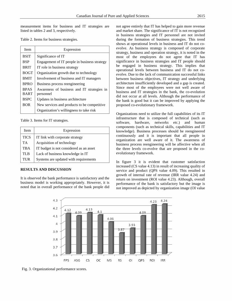
Canadian Journal of Pure and Applied Sciences 2615
measurement items for business and IT strategies are listed in tables 2 and 3, respectively. Table 2. Items for business strategies.
Item Expression
BSIT BSP BRIT BOGT BMIT BPRO BPAS BART BSPC BOR
Significance of IT Engagement of IT people in business strategy IT role in business strategy Organization growth due to technology Involvement of business and IT managers Business process reengineering Awareness of business and IT strategies in personnel Updates in business architecture New services and products to be competitive Organization’s willingness to take risk
Table 3. Items for IT strategies.
Item Expression
TICS TA TBA TLB TUR
IT link with corporate strategy Acquisition of technology IT budget is not considered as an asset Lack of business knowledge in IT Systems are updated with requirements
RESULTS AND DISCUSSION It is observed the bank performance is satisfactory and the business model is working appropriately. However, it is noted that in overall performance of the bank people did
not agree entirely that IT has helped to gain more revenue and market share. The significance of IT is not recognized in business strategies and IT personnel are not invited during the formation of business strategies. This trend shows at operational levels in business and IT do not co-evolve. As business strategy is composed of corporate strategy, business and operation strategy, it is noted in the most of the employees do not agree that IT has significance in business strategies and IT people should be engaged in business strategy. This implies that operational levels between business and IT do not co-evolve. Due to the lack of communication successful links between business objectives, IT strategy and underlying architecture insufficiently developed and a gap is created. Since most of the employees were not well aware of business and IT strategies in the bank, the co-evolution did not occur at all levels. Although the performance of the bank is good but it can be improved by applying the proposed co-evolutionary framework. Organizations need to utilize the full capabilities of its IT infrastructure that is composed of technical (such as software, hardware, networks etc.) and human components (such as technical skills, capabilities and IT knowledge). Business processes should be reengineered continuously and it is important that all people in organization are well aware of it. The awareness of business process reengineering will be affective when all the three levels co-evolve that are proposed in the co-evolutionary framework. In figure 3 it is evident that customer satisfaction increased (CS value 4.13) in result of increasing quality of service and product (QPS value 4.09). This resulted in growth of internal rate of revenue (IRR value 4.24) and return on investment (ROI value 4.23). Although, overall performance of the bank is satisfactory but the image is not improved as depicted by organization image (OI value
Fig. 3. Organizational performance scores.

Khan 2616
3.93). This data may be complemented with RS (value 3.87) where staff members are not rewarded based on their performance. Figure 4 shows that majority of the employees agree that business process reengineering (BPRO value 4.15) is necessary for business effective performance. This is supported by another item business architecture BART (value 4.13) in which people agree the business architecture needs to be changed in order to be aligned with the underpinning technologies. However, significance of IT in business BSIT (value 2.52) is not considered within the bank as most of the employees did not recognize it. This is also supported by BSP (value 2.67) where employees do not agree to engage IT personnel in business strategy. This shows absence of co-evolution in both business and IT. In figure 5 the item TBA (value 4.13) shows that people do not consider IT as an asset for the bank and this also
shows the gap between business executives and IT personnel. Co-evolution in organization may not occur unless the evolving business processes are supported by the evolving technologies. As depicted in figures 4 and 5 that most of the respondents consider IT budget as an expense (item TBA) that is the organization does not value the adaptation of technologies. This argument is supported by the data TUR and TA as well where new technologies are not readily acquired and updated with the new systems. The data shows the information systems in the bank are updated with the existing technologies due to financial restrictions. This also depicts that co-evolution does not occur effectively as when business and IT strategies are changed the lower levels do not co-evolve due to budget constraints and therefore, a misalignment occurs. This also validates the co-evolutionary framework that requires co-evolution from first level to the third level.
Fig. 4. Business strategies scores.
Fig. 5. IT strategies scores.

Canadian Journal of Pure and Applied Sciences 2617
The case of the bank illustrates that there is development in business as a result of business evolution (new services and products), but due to absence of evolving IT there is a gap between business and IT. Co-evolution in the bank may occur in result of a change that requires changes in all levels and components. Currently co-evolution does not occur since the architecture of the bank does not co-evolve i.e. when the new services or products are introduced or new business strategies are adopted, the supporting technologies do not co-evolve. Secondly, the absence of appropriate communication between business and IT people at all levels causes the misalignment and does not allow co-evolving the system and the gap between the two entities arises. CONCLUSION The purpose of this research study was to develop a co-evolutionary framework by integrating three levels i.e. strategic level, operational level and individual level. The three levels have been integrated by a k-mediator that facilitates co-evolution between levels of each entity. The benefit of the framework is that it ensures the co-evolution occurs at all three levels of business and IT. Therefore, business processes will become more efficient and effective in order to fulfil clients’ requirements and more revenue generated. The findings show that the co-evolution does not occur at all levels and the data obtained from different measurements exhibit good validation of the framework. REFERENCES Agarwal, R. and Sambamurthy, V. 2002. Principles and Models for Organizing the IT Function. MIS Quarterly Executive. March, (available at http://misqe.org/V0101-02.pdf).
Aier, S. and Winter, R. 2009. Virtual Decoupling for IT/Business Alignment–Conceptual Foundations, Architecture Design and Implementation Exampl. In: Business & Information Systems Engineering. 51(2):150-163.
Anderson J. 2001. Information Technology Strategic Decision Making Approaches and Organizational Performance in different Industrial Settings. Journal of Strategic Information Systems,(10). 101-119
Aversano L., Bodhuin T. and Tortorella M. 2005. Assessment and Impact Analysis for Aligning Businesses Processes and Software Systems. SAC’05 ACM, NM
Benbya, H. and McKelvey, B. 2006. Using Coevolutionary and Complexity Theories to Improve IS Alignment: A Multi-level Approach. Journal of Information Technology. 21:284-298.
Burgelman, A. 1994. Fading memories: A process theory of strategic business exit in dynamic environments. Administrative Science Quarterly. 39(1):24-5.
Carmines, E. and Zeller, R. 1979. Reliability and Validity Assessment. SAGE Publications.
Cragg, P., King, M. and Hussin, H. 2002. IT Alignment and Firm Performance in Small Manufacturing Firms. Journal of Strategic Information Systems. 11:109-132.
Cronford, T. and Smithson, S. 1997. Project Research in Information Systems: As Student’s Guide. London Macmillan Press.
Croteau, M. and Bergeron, F. 2001. An Information Technology Trilogy: Business Strategy, Technological Deployment and Organizational Performance. Journal of Strategic Information Systems. 10(2):77-99.
Curtis, B., Kellner, I. and Over, J. 1992. Process Modelling. Communications of the ACM. 35(9):75-90.
Ehrlich, R. and Raven, H. 1964. Butterflies and plants: a study in co-evolution. Evolution. 18:568-608.
Gunsekaran, A., Peter, D., Rahimi, F. and Miele, R. 2001. A Model for Investment Justification in Information Technology Projects. International Journal of Information Management. 21:349-364.
Henderson, C. and Venkatraman N. 1999. Strategic Alignment: Leveraging information technology for transforming organizations. IBM Systems Journal. 38: 472-484.
Jan, S., Ulrik, F., Robert, L. and Mathias, E. 2010. Enterprise Architecture Meta Models for IT/Business Alignment Situations. In: Proceedings of 14th International Enterprise Distributed Object Computing Conference, Brazil. 14-23.
Kauffman, S. 1993. The Origins of Order: Self-organization and selection in Evolution. Oxford University Press.
Khan, MA. 2012. Analysis of Organizational Factors that Impact the Gap between Business and Information Technology. European Journal of Scientific Research. 68(2):154-160.
Khan, MA. and Zedan, H. 2010. Alignment Strategies and Frameworks in Co-Evolution of Business and Information Technology. In: Proc. IEEE International Conference on Information, Networking and Automation (ICINA’10). VI-133-136.
Koza, P. and Lewin, A. 1998. The Co-evolution of Strategic alliances. Organization Science. 9:255-264.
Martin, J., Jens, W. and Werner, E. 2010. A Model-Driven Framework for Business IT Alignment. Int. J. Internet and Enterprise Management. 6(3):233-247.

Khan 2618
McKelvey, B. 1999. Self-organization, complexity, catastroph, and microstate models at the edge of chaos. In: Variations in organization science. Eds. Baun, JAC. and McKelvey, B. In honor of Donald T. Campbell, Thousand Oaks, CA, Sage. 279-307.
Morrison, R., Balasubramaniam, D., Kirby, G., Mickan, K., Wardboys, B., Greenwood, R., Robertson, I. and Snowdown, B. 2007. A framework for supporting dynamic systems co-evolution. Autom Softw Eng. 14: 261-292.
Nunnaly, C. and Bernstein, H. 1994. Psychometric Guide (2nd ed.), McGraw Hill, New York, USA.
Papp, D. 2004. Assessing Strategic Alignment in Real Time. Journal of Informatics Education Research.
Rathnam, G., Justin J. and Joseph, H. 2005. Alignment of Business Strategy and IT Strategy: A case study of fortune 50 financial services company. Journal of Information Systems. 45(2):1
Reich, H. and Benbasat, I. 2000. Factors that Influence the Social Dimension of Alignment between Business and Information Technology Objectives. Management Information Systems Quarterly. 24:81-113.
Sabherwal, R. and Chan, E. 2001. Alignment between Business and IS Strategies: A Study of Prospectors, Analyzers and Defenders. Information Systems Research. 12(1):11-33
Strnadl, F. 2006. Aligning Business and IT: The Process-Driven Architecture Model. Information Systems Management. 23(4):67-77.
Tallon, P. 2007. Process-oriented Perspective on the Alignment of Information Technology and Business Strategy. Journal of Management Information Systems. 24(3):227-268.
Tivnan, F. 2005. Coevolutionary Dynamics and Agent-Based Models in Organization Science. Proc. of 2005 Winter Simulation Conference.
Zedan, H., Zhou, S., Sampat, N., Chen, X., Cau, A. and Yang, H. 2001. K-Mediator: Towards Evolving Information Systems. IEEE International Conference on Software Maintenance (ICSM’01). 520-527.
Received: Feb 12, 2013; Accepted: Aug 20, 2013

SENRA Academic Publishers, British Columbia Vol. 7, No. 3, pp. 2619-2627, October 2013 Online ISSN: 1920-3853; Print ISSN: 1715-9997
SYNTHESIS, ANTIBACTERIAL AND TOXICOLOGY STUDY OF MN(II), CO(II) AND NI(II) METAL COMPLEXES OF SULFADOXINE
MIXED WITH PYRIMETHAMINE
*Ogunniran, KO1, Adekoya, JA1, Siyanbola, TO1, Ajayeoba, TA2 and Inegbenebor, AI1 1Department of Chemistry, College of Science and Technology, Covenant University, Ota, Ogun State
2 Department of Chemistry, Faculty of Science, Obafemi Awolowo University, Ile-Ife, Osun State, Nigeria
ABSTRACT Three mixed ligand metal complexes of Sulphadoxine and Pyrimethamine were prepared by using Mn(II), Ni(II) and Co(II) metal chloride hexahydrate and characterized by elemental analysis, molar conductivity, magnetic susceptibility measurement, AAS, IR and UV-Vis. spectroscopy. Some physical parameters were obtained using molar conductance measurement and melting point determination. Based on the analytical and spectroscopic data, the complexes were proposed to have the formulae: [ML1L2](Cl)2 (where M = Mn(II), Ni(II) and Co(II); L1 = sulphadoxine, L2 = pyrimethamine). The spectroscopic data proposed that L1 and L2 coordinated through N of NH2 groups in L1 and through N atom of NH group in L2. Thus, pyramethamine was proposed to be a tridentate ligand, while sulphadoxine was proposed to be a monodentate ligand. Micro-analysis further supported the proposed structure for the complexes. The antibacterial activity of the metal complexes were compared with their ligands by screening them against isolates of some strains of g(-) Escherichia coli, g(+) Proteus sp., g(+) Pseudomonas aureginosa and Salmonella typhi by using diffusion method. The results obtained showed the metal complexes to be more potent antibacterial than the parent drugs against the four species used. Toxicology tests against some tissues of albino rat (Rattus novergicuss) revealed toxicity of the complexes in the kidney as compared to the parent drugs. However, ALP values for metal complexes were found to be non-significantly different from the ALP values obtained for livers and the sera. This indicates that the metal complexes are not excessively toxic. Keywords: Metal complexes, complexation, antibiotics, antimicrobial properties, alkaline phosphatase. INTRODUCTION Vector borne infectious diseases are rapidly spreading in tropical and sub-tropical regions including parts of the America, Asia and Africa (Mendis et al., 2006). These diseases results in millions of death across the globe annually. The spread of infectious diseases is not just associated with poverty but also serve as major hindrance to economic development (Ajibade, 2008; Sachs and Malaney, 2002). Although, many chemotherapic agents are in the market, there is tremendous increase in the ability of the parasite to survive or multiply despite the administration and absorption of drugs. This is generally accepted to be initiated primarily through a spontaneous mutation that reduces level of sensitivity of the drug. Also, biological mechanism behind the resistance was subsequently reported to be related to the development of an efflux mechanism that expels the drug from the parasite before reaching the required concentration that will effectively inhibit the process of heme polymerization (Elzahany et al., 2008; Shiva et al., 2012). Antimicrobial resistance is fast becoming a global concern with rapid increase in multidrug resistance in bacteria. Thus, some previously treatable pathogens are
now becoming untreatable. Pyramethamine is notably used in the treatment of chloroquine-resistant cases of malaria due to Plasmodium faciparum in combination with sulfadoxine (Trampuz et al., 2003). Compounds containing pyrimidine rings have been reported to possess biological activities (Morad et al., 2007). Many therapeutic agents contain pyrimidine ring which enable them to coordinate with metal ion in the body system. Resistance of P. faciparum to first line treatment drugs have become a major concern for developing countries. Therefore, it has become highly imperative to prepare possible new antibacterial agents that can serve as future replacement for the present crop of drugs. However, the medicinal uses and applications of metals complexes are of increasing clinical and commercial importance. The essential trace metals cannot be over emphasized in a living system. Transition metal ions are responsible for the proper functioning of different enzymes (Farrell, 2003; Roat-Malone, 2007). In our effort to search for novel chemotherapeutic drugs against parasitic diseases, we reported the synthesis, characterization, antimicrobial and toxicology study of Co(II), Mn(II) and Ni(II) complexes of pyramethamine mixed with sulfadoxine.
Corresponding author email: [email protected]

Ogunniran et al. 2620
MATERIALS AND METHODS Pyramethamine and sulfadoxine were obtained from Bond Chemicals, Lagos, Nigeria. They are products of Sigma Chemical Company, USA. All the solvents and other reagents were of high purity (Aldrich and Sigma products) and were used without further purification. CoCl2.6H2O, NiCl6.6H2O and MnCl2.6H2O were used as metal ion sources. Isolates of gram (-) Escherichia coli, gram (+) Staphilococcus aureus, gram (+) Pseudomonas aureginosa and gram (+) Salmonella typhi were obtained from Microbiology Department, Covenant University, Nigeria. Albino rats (Rattus novergicus) obtained from Chemistry Department, University of Ilorin were used for toxicology study. Experimental methods IR spectra of the samples in KBr pellets were obtained in the ranges of 400 to 4000 cm-1 on Thermo Nicolet FTIR spectrometer. Metal analyses were determined by AAS on Thermo S Series AAS. The analyses of carbon, hydrogen, oxygen and nitrogen were carried out on a Perkin–Elmer 204C micro analyzer, UV-Vis spectra were obtained on Thermo Genesys IOVV Scanning UV-Vis spectrometer. Magnetic moment was carried out by using Faraday balance. The melting point determination was carried out using Gallenkamp melting point apparatus. Conductivity measurement was carried out using CON 6/TDS6 Handheld Conductivity/TDS meter with DMF as solvent. Synthesis of metal complexes 0.6206g (2mmol) of sulfadoxine and 0.5000g (2mmol) of pyrimethamine were dissolved in 20ml of ethanol separately (Martak et al., 2009). The solutions were mixed thoroughly together in round bottom flask. The resulting mixture was stirred under reflux for 1 h, after which 0.01 mol. of each of the metal salt in 20ml methanol was added. The reaction mixture was refluxed for 3 h, after which the solution was allowed to cool to room temperature and left on the bench for 2 weeks. The crystals formed were filtered under vacuum, washed twice with ethanol and dried in desiccator containing CaCl2 as drying agent. Purity of the compounds was confirmed by using thin layer chromatography (TLC). Antimicrobial study The inhibitory activity of the ligands and the metal complexes were determined by screening their antibacterial activity against pathogenic bacterial species like gram (-) E. coli, gram (+) S. aureus, gram (+) P. aureginosa and gram (+) S. typhi (Collins and Lyne, 1980; Garba and Salihu, 2011). Isolates of the bacteria were cultured in nutrient broth and incubated at 37°C for 24h. Sulphadoxine and pyramethamine were used as standard while only methanol was used as control. Nutrient agar (5g nutrient broth; 3.1g of nutrient agar in 200ml of sterile water for 8 plates) was prepared as the
basal medium for the cultured bacteria and autoclaved. 1.0cm diameter wells were punched and 0.1ml of sterile solutions of each of the compounds (1.0w/v) was applied to each well and incubated at 37.1°C for one to three days. The observed zone of inhibition (in mm) is presented as mean ± SEM in figures 1 to 4.
Average diameter of bacterial colony on the test plate (mm)
% Inhibition= Average diameter of growth of bacterial colony on the control plate (mm)
× 100
Toxicology study In order to compare the level of toxicity of the metal complexes with the ligands, 30 albinos rats weighing between 150 and 170g were used for toxicology study (Ogunniran et al., 2007, 2008). Enzyme activity (ALP) and protein concentration in the livers, kidneys and sera were determined as described by Tella and Obaleye (2010). Statistical analysis Statistical significance was determined using Duncan multiple range test and the values were considered statistically significant at P< 0.05. RESULTS AND DISCUSSION Physical characteristics and micro analytical data of the ligands and complexes are given in table 1. The analytical data confirmed the proposed formula of the complexes. The results of C,H,O and N percentage are in accordance with the composition suggested for most of the complexes. This is supported by the results of metal content analysis, which correlate with the calculated values. The presence of chloride ion inside the coordination sphere was confirmed by lack of white precipitate of AgCl with the use of AgNO3 solution (Vogel, 1989). Hence, the proposed synthetic equation for the synthesized complexes could be represented as: MCl2.6H2O + L1 + L2 → ML1L2Cl2 + 6H2O Where M = Mn(II), Co(II) and Ni(II), L1 = sulphadoxine, L2 = pyrimethamine The complexes were found to be soluble in methanol and slightly soluble in acetone, chloroform, dimethyformamide, dimethysulfoxide and benzene. However, they were found to be non-soluble in distilled water, ethanol, n-haxane and display good stability in air at room temperature. The molar conductance of 10-3 M solutions of the ligands and metal complexes in DMF are in the range 12.37 to 19.29 Ωcm2mol-1 indicating their non-electrolytic nature (Vogel, 1989). The complexes are of average percentage yield range of 44 to 58 which indicate that they can be synthesized commercially. The

Canadian Journal of Pure and Applied Sciences 2621
complexes were found to possess higher melting point as compared to the ligands. The increase in melting point is attributed to increase in molecular weight of the complexes due to coordination of metal ions to the ligands (McCleverty and Meyer, 2003). Infrared spectra The infra-red spectra of the ligands were compared with those of the metal complexes (Table 2). They showed similar bands as expected. The strong band in the region 3682 to 3600cm1 in sulfadoxine spectrum assigned to ν(NH) (Salisu et al., 2009; Vogel, 1989; Fessenden and Fessenden, 1990) also, it appeared as strong bands at 3600 and at 3340 cm-1 in pyrimethamine spectrum. Similar bands were observed in metal complexes at lower wavelengths coupled with reduction in intensities. The observations have been attributed to coordination of the vibrational group to the central metal ion (Nora, 2011). This probably account for reduction in intensities of the
bands. The assignment is supported by (C-N) bending vibration observed as medium band at 1170 and 1080cm-1 in sulphadoxine and pyrimethamine spectrum, respectively (Watson, 2000). The band has shifted to higher wavelength in the spectra of metal complexes with reduction in intensity. Other bands assigned to vibrational groups like ν(C=C), ν(S=O) and ν(C-H) in the ligands were also observed with shift in their region of absorption in the spectra of metal complexes as a result of effect of complexation on them. However, M→L bands which were found in the range of 500 to 780cm-1 in the spectra of metal complexes were conspicuously absent in the spectra of the ligands (Obaleye et al., 2001; Ajibade, 2008). Electronic spectral and magnetic studies The electronic spectra of sulphadoxine (Table 3) showed two absorption bands at 49505 and 36900cm-1. The bands were assigned to π-π* of the phenyl rings in the ligand
Table 1. Colour, decomposition temperature, conductivities and analytical data of the ligands L1 and L2 and their mixed ligands metal complexes.
Compound % C
found (Calc)
% H Found (Calc)
% O Found (Calc)
% N Found (Calc.)
Metal found (Calc)
Conductivity Ω-
1cm2mol-1
M.Pt. °C
Colour/ state
Yield (%)
Sulfadoxine (L1) (46.44) 46.17
(4.22) 4.01
(20.62) 20.32
(18.06) 18.03 - 14.55 191-192 -
Pyramethamine (L2)
(57.95) 57.89
(4.46) 4.44 - (22.52)
22.50 - 12.37 193-194 -
Mn(L1L2)Cl2 (42.08) 42.01
(3.52) 3.44
(9.34) 9.30
(16.36) 16.11
(8.02) 7.96 19.14 205 White
crystal 44
Co(L1L2)Cl2 (41.84) 41.32
(3.51) 3.49
(9.29) 9.22
(16.26) 16.17
(8.55) 8.45 18.14 265
Light pink
powder 58
Ni(L1L2)Cl2 (41.86) 41.81
(3.51) 3.48
(9.29) 9.27
(16.27) 16.22
(8.52) 8.31 19.29 245
Light green
powder 51
Table 2. IR Spectra (4000-400 cm-1) of the ligands L1 and L2 and their mixed metal complexes.
Compound ν (N-H) cm-1
ν (C-H) cm-1
ν (C=C) cm-1
ν (C-N) cm-1
ν (C-O) cm-1
ν (S=O) cm-1 M→L
L1 3682 s 3600 s 3010s,b 1580 s 1170 m 1210 s,b 1190 s -
L2 3605 s 3410 s 3010s,b 1600 s
1510 s 1080 m 1220 s,b - -
Mn(L1L2)Cl2 3620 m 3340 m 3005.01s 1605 s
1510 s 1430 vw 1430 w 1250 s 1200 s,b 500 s
Co(L1L2)Cl2 3602 m 3005.01s 1560 s 1510 m 1310 vw 1310 w 1225 s,b 500 m
Ni(L1L2)Cl2 3600 s
3405 m,b 3105.02s 1600 m 1520 m 1410 s 1410 s 1200 s,b 780 vs
w- Weak, s- strong, m- medium, vw- very weak, vs-very strong, m,b- medium and broad, s,b- strong and broad.

Ogunniran et al. 2622
due to conjugation (Vogel, 1989). Similar bands were observed at 49505 and 34965cm-1 286nm in the pyrimethamine spectrum. However, these bands were observed in the metal complexes to have shifted to higher wavelength due to complexation (Ajibola et al., 1998). Extra bands observed in Mn(II), Co(II) and Ni(II) complexes were attributed to d-d transition. The intense green colour of Ni(II) complex showed three weak absorption bands at 24272, 25907 and 26810cm-1 due to the splitting of ground 3F term and the presence of the 3P term. The absorption bands were attributed to 3A2g(F) → 3T2g(F), 3A2g(F) →3T2g(F) and 3A2g(F) → 3T1g(P) respectively. The broad peak absorption bands observed indicate large distortion from octahedral symmetry, as a result of which unsymmetrical bands were observed. However, magnetic moment value of 3.17 BM obtained
for the complex is within the octahedral environment range of 2.8-3.5 BM. Thus, the complex could be distorted octahedral (Cotton and Wilkinson, 1985). The electronic spectra of Co (II) complex displayed three absorption bands assigned to 3T1g(F) → 3T2g, 3T1g(F) → 3T1g(P) and 3T1g(F) → 3A2g transitions respectively. These bands are characteristics of high spin octahedral Co(II) complex. The magnetic measurement of Co(II) complex exhibited magnetic moment value of 4.64 BM which is within the octahedral range of 4.3 - 5.2 BM. Mn(II) complex showed absorption bands at 20576, 25510 and 34722cm-1. The bands were assigned to 6A1g → 4T1g(G), 6A1g → 4T2g(G) and 6A1g → 4T2g(D) transitions respectively. The complex exhibit magnetic moment of 5.82 BM, which supported octahedral geometry around Mn (II) ion (Fahmideh et al., 2010).
Table 3. UV-Vis. Spectra assignments of sulphadoxine, pyramethamine and their mixed metal complexes and magnetic moment measurements of the metal complexes.
Compounds Wavelength (nm) (cm-1) Assignment Magnetic moment
(BM)
L1 202 271
49505 36900
π-π* n-π*
L2 202 286
49505 34965
π-π* n-π*
Mn(L1L2)Cl2 486 392 288
20576 25510 34722
6A1g→4T1g 6A1g →4T2g(G) 6A1g →4T2g(D)
5.82
Co(L1L2)Cl2 443 317 342
22573 31546 29240
3T1g(F)→3T2g 3T1g(F)→3T1g(P)
3T1g(F)→3A2g
4.64
Ni(L1L2)Cl2 412 386 373
24272 25907 26810
3A2g(F)→3T2g(F) 3A2g(F)→3T2g(F) 3A2g(F) →3T1g(P)
3.17
g- Gerade.
N
N
NHHN
Cl
MCl Cl
HN
S
O
O
N
H OCH3
OCH3
N N
Where M= Mn(II), Co(II) and Ni(II) Structure 1. The proposed structure of the prepared complexes.

Canadian Journal of Pure and Applied Sciences 2623
Suggested structural formulae of the complexes From the spectral data and the elemental analyses, the proposed structure of the prepared complexes is as shown in Structure 1. Biological study In vitro antibacterial activities of the ligands were compared graphically to those of the mixed ligands metal complexes (Figs. 1 to 4). From the results obtained, it can be concluded convincingly that the metal complexes are more active than the ligands against all the bacteria used. Increase in activity observed could be attributed to coordination of the ligands to metal ions. However, Ni(L1L2)Cl2 was found to be less active against g(+) S. typhi (Fig. 4). This observation could be as a result of
ability of the bacterium to develop efflux mechanism against the complex (Barbara et al., 2010; Ajibade, 2008). It could also be as a result of effect of coordination on the active site in the complex (Heslop and Jones, 1986). The overall results confirmed that the metal complexes are more potent than the parent ligands under identical experimental conditions. This would suggest that the chelation could facilitate the ability of a complex to cross a cell membrane and can be explained by Tweedy's chelation theory (William, 1981). Results of toxicology assay The values of ALP activities in the kidney, liver and serum following the administration of ligands and their mixed metal complexes as compared to the control are
Fig. 1. Zone of inhibition (%) of the ligands and metal complexes against E. coli.
Fig. 2. Zone of inhibition (%) of the ligands and metal complexes against Proteus species.

Ogunniran et al. 2624
shown in figures 5 to 7. The results indicated that kidney (Fig. 5) produced significant increase (P<0.05) in ALP activities as compared to the control value. Sulp and pyra produced non-significant difference as compared to control value. This is an indication that increase in their enzyme activity did not lead to damages to plasma membrane of the organ (Ogunniran et al., 2007). However, administration of the metal complexes increased the enzyme activity beyond tolerance level (75.62 to83.79 nM/min/mg protein) in the kidney and thus produced significantly different values as compared to control value. The trend confirmed alteration in the enzymes activity of the kidneys which may likely cause damage to their plasma membrane (Yakubu et al., 2005). It may also be attributed to induction in enzyme synthesis
which leads to hydrolysis of phosphate ester of the organ and other essential cells (Roat-Malone, 2007). The damages of the tissue cell plasma membrane may lead to leakages of membrane components into the extracellular fluid (Yakubu et al., 2005). The ALP activities values for sera and livers (Figs. 6 and 7, respectively) of the rats administered with metal complexes were found to be non-significantly (P<0.05) different from control values. The non-significant changes observed in ALP activity of the liver and serum suggested partial non-damage effect of the metal complexes in them. It can therefore be concluded that even though the metal complexes are toxic than the parent ligands, they can still be tolerated in the body system.
Fig. 3. Zone of inhibition (%) of the ligands and metal complexes against P. aureginose.
Fig. 4. Zone of inhibition (%) of the ligands and metal complexes against S. typhi.

Canadian Journal of Pure and Applied Sciences 2625
CONCLUSION This study shows feasibility and justification for synthesis of mixed antibiotics metal complexes using sulphadoxine and pyramethamine as ligands. The complexes possessed better physical properties and are more effective as chemotherapy agents than their parent antibiotics. However, the complexes are toxic at the dose level used to the kidneys but not to livers and sera of the rat administered with the complexes. Thus, the present study concluded that complexes could be used as good drug of choice to manage the bacterial diseases after evaluating the in vivo effect of metal complex on experimental higher animal and clinical trials.
REFERENCES Ajibade, P. 2008. Metal complexes in the management of parasitic diseases: In vitro antiprotozoal studies of metal complexes of some antimalarial drugs. Current Science. 95(12):28. Ajibola, AO., Ogundaini, AO, Ayin, JS. and Olugbade, TA. 1998. Essential Inorganic and Organic pharmaceutical Chemistry (2nd ed.). Sathron Associates Ltd. 79-85. Barbara, O., Michał, F., Agnieszka, E. and Bohdan, JS. 2010. Synthesis and antibacterial activity of new trimethoprim analogue. Science24.com/conference. pp27. Collins, CH. 1980. Microbiological Methods (3rd ed.). Butterworths and Co. Ltd. 414-427.
Fig. 5. Results of toxicology test of the ligands and metal complexes against kidney homogenate.
Fig. 6. Results of toxicology test of the ligands and metal complexes against liver homogenate.

Ogunniran et al. 2626
Cotton, FA. and Wilkinson, G. 1985. Advanced Inorganic Chemistry, (4th ed.). John Willey and Sons. 628-641.
Elzahany, EA., Hegab, KH., Safaa, KH. and Youssef, NS. 2008. Complexes with Schiff Bases Derived from 2-Formylindole, Salicyladehyde, and N-amino Rhodanine. Australian Journal of Basic and Applied Sciences. 2(2):210-220.
Fahmideh, S., Lotf, Ali, S. and Shahriar, G. 2010. Synthesis, characterization and anti-tumour activity of Fe(III) Schiff base complexes with unsymmetric tetradentate ligands. Bull. Chem. Soc. Ethiop. 24(2):193-199.
Fessenden, RJ. and Fessenden, JS. 1990. Organic Chemistry, (4th ed.). Harness and Nabie Inc., USA. 1048.
Heslop, RB. and Jones, K. 1986. Inorganic Chemistry, A guide to Advance Study (3rd ed.). Elsevier Scientific Pub. Co., England. 284:541-544.
Li-june, M. 2003. Structure and function of metallo-antibiotics. Med. Res. Rev. 23:697-762.
McCleverty, JA. and Meyer, TJ. 2003. Comprehensive coordination chemistry II: From Biology to Nanotechnology (2nd ed.). 8:232-236.
Mendis, K., Sina, B., Marchesini, P. and Carter, R. 2006. The neglected burden of Plasmodium vivax malaria. Am. J. Trop. Med. Hyg. 64(1-2):97-106.
Morad, FM., Elajaily, MM. and Ben Gweirif, S. 2007. Preparation, Physical Characterization and Antibacterial Activity of Ni (II) Schiff Base Complex. Journal of Science and Its Applications. 1:72-78.
Nora, HA. 2011. Synthesis, Characterization and Biological Activities of Cu(II), Co(II), Mn(II), Fe(II), and UO2(VI) Complexes with a New Schiff Base Hydrazone: O-Hydroxyacetophenone-7-chloro-4-quinoline Hydrazone. Molecules. 16:8629-8645; doi:10.3390/ molecules16108629.
Obaleye, JA., Adeyemi, OG. and Balogun, EA. 2001. Some metal tetracycline complexes: synthesis, characterization and their effects against malarial parasites. Int. J. Chem. 11(2):101-106.
Ogunniran, KO., Ajanaku, KO., James, OO., Ajani, OO., Adekoya, JA., Omonhimin, CA. and Allensela, MA. 2008. Synthesis, physical properties, antimicrobial potentials of some mixed antibiotics complexed with transition metals and their effects on alkaline phosphatase activities of selected rat tissues. Scientific Research and Essay. 3(8):348-354.
Ogunniran, KO., Tella, AC., Alensela, M. and Yakubu, MT. 2007. Synthesis, physical properties, antimicrobial potentials of some antibiotics complexed with transition metals and their effects on alkaline phosphatase activities of selected rat tissues. African Journal of Biotechnology. 10(6):1202-1208.
Prashanthi, Y., Kiranmai, K., Sathish Kumar, K., Chityala, VK. and Shiva, R. 2012. Spectroscopic Characterization and Biological Activity of Mixed Ligand Complexes of Ni(II) with 1,10-Phenanthroline and Heterocyclic Schiff Bases. Bioinorg hem Appl. doi: 10.1155/2012/948534.
Roat-Malone, RM. 2007. A short course, Bioinorganic Chemistry (2nd ed.). John Wiley & Sons, Inc. 3-9.
Fig. 7. Results of toxicology test of the ligands and metal complexes against sera.

Canadian Journal of Pure and Applied Sciences 2627
Sachs, J. and Malaney, P. 2002. The economic and social burden of malaria. Nature. 415:680-685.
Tella, AC. and Obaleye, JA. 2010. Synthesis of Some 3d Metal Complexes of Quinine and Their Toxicological Studies. J. Nepal Chem. Soc. 25:19-28.
Trampuz, A., Jereb, M., Muzlovic, I. and Prabhu, R. 2003. Clinical review: Severe malaria. Crit. Care. 7(4):315-23.
Vogel, T. 1989. In: Vogel Textbook of Practical Organic Chemistry (4th ed.). John Wiley Inc., England. 133-325.
Watson, DG. 2000. Pharmaceutical analysis: A textbook for pharmacy students and pharmaceutical chemists. Churchill Livingstone (2nd ed.). 3-17.
William, OF. 1981. Pinciples of medicinal chemistry (2nd ed.). Lea and Febiger, Philadelphia. 779-798.
Yakubu, MT., Akanji, MA. and Oladiji, AT. 2005. Aphrodisiac potentials of aqueous extract of Fadogia agrestis (Schweinf. Ex Heirn) stem in male albino rats. Asian J. Androl. 7(4):399-404.
Received: May 14, 2013; Accepted: June 7, 2013

SENRA Academic Publishers, British Columbia Vol. 7, No. 3, pp. 2629-2633, October 2013 Online ISSN: 1920-3853; Print ISSN: 1715-9997 Short Communication
ELEMENTAL CONTENT OF MANUFACTURED SOILS
*Maria V Kalevitch1, Paul Badger1, Bill Dress1 and Valentine I Kefeli2
1Robert Morris University, 6001 University Blvd., Moon twp, PA 15108, USA 2Biomost, Inc., PA, USA
ABSTRACT
Information on plot-specific background concentrations of trace metals in manufactured soils is critical for evaluating performance of soil manufacturing recipes and for monitoring the annual bio-availability of trace metals. In this project, total concentrations of trace metals (Cu, Fe, Mn, Ni, Pb, and Zn) and macro nutrients (Ca, Mg, K, P, N) in manufactured soil samples were determined. Seven soil samples were analyzed for pH, cation exchange capacity (CEC), extractable phosphate and sulfate, total concentrations of trace metals (Cu, Fe, Mn, Ni, Pb, and Zn) and macro nutrients (Ca, Mg, K, P). A subset of these metals (Cu, Fe, Mn, Ni, and Pb) are indicators of contamination by acid mine drainage or manufacturing byproducts in the manufactured soil recipe. Average precision for elements Cu, Mg, Fe, Mn, K, and Zn were < 15% relative standard deviation (RSD) using Method 3051.
Keywords: Manufactured soils, trace elements, soil health and sustainability.
INTRODUCTION The present study is the continuation of years of discussion and study of the effects of manufactured soils on soil/plant health. The size consistency (soil texture) of the mineral fraction in native soil varies from clay-size to coarse sand-size. The carbon- and nitrogen-rich organic matter contains the monomers and polymers, the main constituents of the humus complex. Soil is a necessary intermediate substrate in the regulation of the Biosphere activity. Estimates of the loss of US soil resources due erosion to range from 2 billion to 6.8 billion tons annually (GAO, 1977; Barlowe, 1979). Worldwide estimates indicate that between 10-15 million hectares of arable land are rendered unproductive annually due soil losses (Lal and Stewart, 1990). Rehabilitation of the soil cover is a global problem that could be solved in cooperation with such disciplines as mineralogy, soil science, biology, ecology, agrochemistry, and biochemistry. Numerous researchers are concerned with the damage that acid mine drainage does to the soil, water, and biological communities. Janzen et al. (2008), described the impact of acid mine drainage on microbial community diversity and stream chemistry in the Shamokin Creek Watershed, PA. It is a well known fact that diatoms as representatives of biodiversity indicate the health of a particular environment. Bacterial presence also indicates the level of ecological balance. The authors concluded that in AMD
where the concentrations of iron are high, the predominant bacteria will be from phylum Bacteroidetes, and were closely related to known biofilm community members from acidic environments where they have been demonstrated to be involved in sulfur oxidation. Other bacterial species were closely related to Sphingomonas species. Soil ecology damage due to AMD has the potential to have a cascade of negative effects including the loss of vegetation leading to the loss of topsoil due to erosion. In our prior study (Kalevitch and Kefeli, 2006), the proposed recipes of fabricated soils are based on the carbon-nitrogen balance in the soil as well as on the transformation of carbon products such as glucose, phenolics, and plant polymers such as cellulose and lignin in the humus (polymers which are tightly connected to the aluminosilicate matrix of the soil micelle). This research continues a long term study of the soil health of an area damaged by AMD. Macronutrients (Summary Table 1) can be broken into two more groups: primary and secondary nutrients. The following macro and micro nutrients were selected for this study in order to assess the overall health of the soil and to trace deficiencies or excesses in nutrient levels. Information on plot-specific background concentrations of trace metals in manufactured soils is critical for evaluating performance of soil manufacturing recipes and for monitoring the annual bio-availability of trace metals. *Corresponding author email: [email protected]

Kalevitch et al.
2630
In this project, total concentrations of trace metals (Cu, Fe, Mn, Ni, Pb, and Zn) and macro nutrients (Ca, Mg, K, P, N) in manufactured soil samples were determined. Subsets of these metals (Cu, Fe, Mn, Ni, and Pb) are indicators of contamination by AMD residue or by manufacturing byproducts in the manufactured soil recipe. The goal of this study is to evaluate the mineral content of soils from an abandoned strip mine site remediated with fabricated soil amendments. MATERIALS AND METHODS Study Site The study site is located in Butler County, Pennsylvania, USA. The site was strip mined in the 1950’s and has experienced acid mine drainage in the subsequent years. The resulting site has remained sparsely vegetated since the original mining. To remediate this site, a fabricated soil amendment, a natural mixture of decaying substrates rich in aluminosilicate, carbon, nitrogen, phosphorus and potassium sources, was added to test plots. Eight soil samples were collected from the reclaimed mining site; seven samples were collected from test plots with fabricated soil or topsoil and one from abandoned mining soil. Sample Analysis Samples were allowed to air-dry and were then crushed and screened to pass through a 2.0 mm-mesh sieve. Soils were analyzed for pH, Cation Exchange Capacity (CEC), total nitrogen, extractable phosphate and sulfate, total
concentrations of trace metals (Cu, Fe, Mn, Ni, Pb, and Zn) and macro nutrients (Ca, Mg, K, P). Soil pH was measured as a slurry at a 1:2 soil/water ratio with a Fisher Accumet 25 pH meter. Cation Exchange Capacity (CEC) was determined following the method of Robertson et al. (1999). Exchangeable ion concentrations were analyzed on a Perkin Elmer AAnalyst 100 utilizing air/acetylene flame with the appropriate hollow cathode lamp utilizing standard conditions and optimized for lamp alignment, burner head alignment, and nebulizer flow. Exchangeable aluminum and acidity was determined by titration of KCl extracts with NaOH. Results from exchangeable ion concentrations and exchangeable acidity were converted to cmol charge per kg dry soil to determine total CEC. Total nitrogen and phosphorous concentrations were determined following digestion according to the method of Parkinson and Allen (1975). After sample digestion, total nitrogen concentrations were determined on a BioTek Elx808 well plate reader according to the method of Sims et al. (1995). Phosphorous concentrations were determined on a BioTek Elx808 well plate reader. Extractable phosphate and sulfate concentrations were determined by ion chromatography (IC) according to a modified Olsen method (Olsen and Summers, 1982). To determine total metal concentrations, samples were digested in a block digester using EPA Method 3050B. AA and AE analysis were completed on a Perkin Elmer AAnalyst 100 utilizing air/acetylene flame with the
Table 1. Importance of Soil Nutrients for Plant Growth.
N Nitrogen helps form amino acids which are building blocks of protein
Cu Copper is necessary for chlorophyll formation and also acts as a catalyst for other plant reactions.
P Phosphorus is utilized in the formation of nucleic acids and other chemicals which help in the development of health root systems, early growth, early maturity and seed production.
Fe Iron also acts as a catalyst for chlorophyll formation and also carries oxygen. It also helps form certain respiratory enzyme systems. These functions make it critical to photosynthesis.
K Potassium is similar to phosphorus in root formation and also appears to promote disease resistance. It increases the size and quality of fruits.
Mn Manganese activates many metabolic reactions in plants and is directly involved in photosynthesis. It accelerates germination and maturity and increases the availability of phosphorus and calcium.
Ca Calcium is used in root system and leaf development and is combined with other elements to form cell walls. It also helps by activating other enzyme systems.
Ni Nickel is a micronutrient which is necessary for proper germination and seed development. (Brown et al., 1987)
Mg Magnesium is the central atom of the chlorophyll molecule which makes it absolutely necessary for photosynthesis. It also plays a role in phosphate metabolism, plant respiration and enzyme systems.
Zn Zinc is necessary for the production of chlorophyll and carbohydrates and aids in the creation of plant growth substances, enzyme systems, and metabolic reactions.

Canadian Journal of Pure and Applied Sciences 2631
appropriate hollow cathode lamp. The instrument was equipped with a 10 cm burner head. All elements were analyzed utilizing standard conditions and optimized for lamp alignment, burner head alignment, and nebulizer flow. Sample concentrations were corrected for matrix effects. Four replicates of each sample were analyzed to determine average concentration and relative standard deviation for each element. Validation of precision and accuracy of methods for trace metals and macro nutrients were performed by two internal standards, an external SRM from the National Institute of Standards and Technology (NIST), and comparison to external analysis results conducted by inductively coupled plasma spectrometry (ICP). Data Analysis Because the study focuses on one specific area within which soil remediation treatments were completed, the study is necessarily qualitative in nature. Results from exchangeable ion concentrations and exchangeable acidity were converted to cmol charge per kg dry soil to determine total CEC. All metal and nutrient concentrations were converted to mg/kg soil for comparison. Soil data was qualitatively compared to historical data from the Butler and Allegheny county region obtained from the USGS PLUTO soils database (http://tin.er.usgs.gov/pluto/soil/) and background concentrations for naturally occurring inorganic chemicals in surface and subsurface soil (Risk Assessment Information System, http://rais.ornl.gov/). RESULTS The evaluation of eight soil samples consisted of testing for the presence of the nine minerals. Five soils represented natural soil with a topsoil cover, two soils were manufactured, and there was also one mineral soil sample taken from a mining soil plot.
Table 2 demonstrates the presence of exchangeable phosphorus and sulfate in the samples along with the cation exchange capacity. According to the background concentrations for naturally occurring inorganic chemicals in surface and subsurface soil (Risk Assessment Information System, http://rais.ornl.gov/) (Table 3), the concentration for calcium in tested soil was well below the normal (200,000 mg/kg), it ranged from 60 to 11,000 mg/kg in different samples (Table 4). The maximum concentration was shown on plot 07-7, and the lowest was for the mining soil plot, 07-8. Table 3. Background Concentrations for Naturally Occurring Inorganic Chemicals in Surface and Subsurface Soil (Risk Assessment Information System, http://rais.ornl.gov/)
Background Valueb Analyte Surface Subsurface Inorganic Chemicals (mg/kg)a
Aluminum 13,000 12,000 Calcium 200,000 6,100 Copper 19 25 Iron 28,000 28,000 Lead 36 23 Magnesium 7,700 2,100 Manganese 1,500 820 Nickel 21 22 Potassium 1,300 950 Zinc 65 60
Concentration for copper ranged from 11.8 to 63 mg/kg with 19 mg/kg being the mean. Five plots had copper concentration higher than normal with two plots being within or below normal range. Concentration of iron (Table 5) was within the normal range: 10,247- 24,300 mg/kg with a mean of 28,000 mg/kg of iron. There was one plot (07-4) where the
Table 2. pH, exchangeable sulfate and phosphate and cation exchange capacity in the Tested Soils (mean +/- standard error).
Soil pH Exchangeable Phosphate (mg/kg soil)
Exchangeable Sulfate (mg/kg soil)
CEC (cmolc/kg soil)
07-1 6.4 6.0 (4) 3.5 (4) 9.5 (1.7) 07-2 5.6 0.8 5.8 (4) 8.5 (1.7) 07-3 8.5 1.7 (0.8) 3.9 (4) 39 (11.0) 07-4 8.4 1.2 (0.6) 5.6 (4) 38 (12.0) 07-5 6.9 36 (13) 6.6 (4) 33 (7.0) 07-6 6.8 32 (13) 10.7 (4) 36 (6.0) 07-7 7.4 181 (4) 48 (11.0) 07-8 3.1 3.8 (1.8) 37 (4) 8.9 (0.5)

Kalevitch et al.
2632
concentration of iron was slightly elevated to 30,000 mg/kg. This, however, is within the relative standard deviation of the measurements. Lead was below normal (>36 mg/kg) in all samples except sample 07-1 that had 60 mg/kg of lead. In seven of the samples manganese concentration varied overall from 29 mg/kg to 1,380 mg/kg which is within the expected background concentrations, however the concentration of manganese in one soil (07-7) was significantly elevated (136,800 mg/kg). Potassium concentration was more than doubled in fabricated and mining soil samples ranging from 2,490 to 3,000 mg/kg. The expected background concentration is 1,300 mg/kg (Table 5). Three soils showed an increase in nickel concentration ranging from 147 to 900 mg/kg vs 21 mg/kg as background. The concentration of zinc was greatest in plot-07-7 (1,300 mg/kg vs 65 mg/kg -normal range), the rest of the samples showed zinc concentrations in the range of 47 to 100 mg/kg. Samples 07-3 and 07-4 had the highest concentration of magnesium 12,300-13,400 mg/kg vs 7,700 mg/kg at the normal range. The rest of the samples had concentrations of magnesium vary from 110-3,700 mg/kg. DISCUSSION Overall, samples collected from the mining site showed the highest concentration of trace elements. They showed
an increase in the following elements: copper, magnesium, iron, manganese, and nickel with concentrations sometimes up to ten times above normal. These soils with elevated mineral contents, especially those with extremely elevated levels zinc and manganese are a concern. For sample 07-7, the concentration of zinc was more than an order of magnitude above the expected value and the concentration of manganese was more than two orders of magnitude above the expected value. This sampling plot was located on an abandoned manganese spoil site. Table 6. Historical soil reference data obtained the USGS PLUTO database (http://tin.er.usgs.gov/pluto/soil/select.php).
Name Butler County
Allegheny County
Calcium (mg/kg soil) 6083.4 4012.78 Cobalt (mg/kg soil) 15.5 17.82 Copper (mg/kg soil) 37.7 52.23 Zinc (mg/kg soil) 100.8 208.00 Magnesium (mg/kg soil) 9229.9 4914.72 Iron (mg/kg soil) 46916.2 50275.21 Lead (mg/kg soil) 23.5 85.27 Potassium (mg/kg soil) 42305.4 32832.68 Nickel (mg/kg soil) 39.2 44.96
In addition to the high levels of zinc and manganese, the concentration of exchangeable sulfate was more than an order of magnitude greater than the normal topsoil samples. Potentially these elevated levels are due to
Table 4. Elemental Analysis for the Tested Soils (mean +/- standard error).
Sample Ca Co Cu Zn Mg 07-1 80 ± 40 19±3 20±3 100±11 1578±100 07-2 20±30 12.2±2 11.8±1 67.1±1 1450±30 07-3 24000±7000 11.8±1 30±20 50±8 12300±1700 07-4 32000±3000 10.4±2 63±4 54.7±2 13400±1600 07-5 7700±800 2±3 24.7±1 47±3 1020±70 07-6 9000±1200 6±7 30±2 51.8±1.1 740±70 07-7 110000±30000 1274±100 20.8±1 1300±50 3700±300 07-8 -60±20 9±5 53.6±1 56±6 100±30
Table 5. Elemental Analysis of the Tested Soils-Continued (mean +/- standard error).
Sample Fe Pb Mn K Ni 07-1 19510±1000 60±30 1310±160 700±120 17±10 07-2 19900±300 30±20 1329±18 710±80 20±13 07-3 24300±1100 6±17 1268±13 1100±500 147±16 07-4 30000±3000 9±18 1380±20 1100±200 180±20 07-5 14800±110 30±30 240±30 2490±160 20±20 07-6 15870±1000 23±11 300±50 2800±200 21±7 07-7 17200±1200 20±30 136800±10000 860±150 900±700 07-8 10247±100 13±3 29±8 3000±200 20±7

Canadian Journal of Pure and Applied Sciences 2633
residual minerals deposited in the soil from the acid mine drainage that originally damaged the area under study. Another potential source for these elevated mineral levels is from the raw materials which were used to create the manufactured soil. Although it is unknown if this is the case for the area under study, in some cases the components used to create the manufactured soil may contain waste sand from casting foundries. Often foundry sands are contaminated with high levels of metals. Further studies are underway to determine the source of these high levels of trace minerals and the effect that they may have on the bacterial ecology within the soil. As the environmental damage caused by acid mine drainage and surface mining operations increases, methods must be developed to repair or replace the topsoil in order to support normal ecological development. As soil is a necessary intermediate substrate in the regulation of the Biosphere activity, it is important to understand the long term effects of micronutrient loss and to monitor attempts to amend soils to improve sustainability and viability of the soil. Future work will compare the mineral content of soil with microbial biomass and diversity. ACKNOWLEDGEMENT We express our sincere appreciation to the group of students who worked tirelessly with us on this project. REFERENCES Brown, PH., Welch, RM., Cary, EE. 1987. Nickel: A Micronutrient Essential for Higher Plants. Plant Physiology. 85:801-803.
Barlowe, T. 1979. Soil Conservation Policies: An Assessment. Soil Conservation Society of America, Ankeny, IA, USA.
General Accounting Office (GAO). 1977. To protect to- morrow's food supply, soil conservation needs priori- ty attention. CED 77-30, GAO, Washington, DC, USA.
Janzen, C., Halke III, D., Evanoski, A., Heath, S., Raithore, S., Holt, J. and Tobin-Janzen, T. 2008. The impact of acid mine drainage mitigation on microbial community diversity and stream chemistry in the Shamokin Creek Watershed. Proceedings 108th Annual ASM Meeting, Boston. pp95.
Kalevitch, M. and Kefeli, V. 2006. Bacterial Presence in Manufactured Soils. Journal of Agricultural, Food, and Environmental Sciences. On-line. Scientific Journals International. 1(1): author insert page numbers here.
Lal, R. and Stewart, BA. 1990. Soil Degradation. Spring- er-Verlag, New York, USA.
Olsen, SR. and Sommers, LE. 1982. Phosphorus. In: Methods of soil analysis, Agron. No. 9, Part 2: Chemical and microbiological properties, (2nd ed.). Am. Soc. Agron., Madison, WI, USA. 403-430.
Parkinson, JA. and Allen, SE. 1975. A wet oxidation procedure suitable for the determination of nitrogen and mineral nutrients in biological material. Communication in Soil Science and Plant Analysis. 6:1-11.
Risk Assessment Information System, http://rais.ornl.gov/.
Robertson, GP., Sollins, P., Ellis, BG. and Lajtha, K. 1999. Exchangeable ions, pH, and cation exchange capacity. In: Standard soil methods for long-term ecological research. Eds. Robertson, GP., Coleman, DC., Bledsoe, CS. and Sollins, P. Oxford University Press, NY, USA.
Sims, GK., Ellworth, TR. and Mulvaney, RL. 1995. Microscale determination of inorganic N I water and soil extracts. Comm. Soil Sci. Plant Analysis. 26:303-316.
USGS PLUTO soils database (http://tin.er.usgs.gov/ pluto/soil/)
Received: May 8, 2013; Revised: Aug 14, 2013;
Accepted: Aug 17, 2013

SENRA Academic Publishers, British Columbia Vol. 7, No. 3, pp. 2635-2638, October 2013 Online ISSN: 1920-3853; Print ISSN: 1715-9997 Short Communication
FABRICATION OF DYE SENSITIZED SOLAR CELL (DSSC) USING ZnO NANOPARTICLES SYNTHESIZED FROM ZINC NITRATE HEXAHYDRATE
Awodugba Ayodeji Oladiran and *Ilyas Abdul-Mojeed Olabisi
Department of Pure and Applied Physics, Ladoke Akintola University of Technology PMB 4000, Ogbomoso, Nigeria
ABSTRACT
DSSC was fabricated using glass as the substrate with copper metal attached to the surface, eosin blue as sensitizer, Lemon juice as electrolyte and ZnO nanoparticles as photoelectrode. The nanostructured ZnO was synthesized by precipitating Zn nitrate hexahydrate with NaOH which was characterized structurally using XRD and optically with a UV-VIS Spectrophotometer. The fabricated DSSC was evaluated and a fill factor of 0.85 obtained with an efficiency of 0.15%. Keywords: UV-VIS, XRD, ZnO, nanoparticles, DSSC. INTRODUCTION The utilisation of renewable energy resources has increased largely in the last years owing to the ever increasing need for electrical energy. The finiteness of fossil fuel used for generation of conventional electrical power on one hand and climate change as a result of the co2 emission by the use of burning those fuels on the other hand. This has led to an indispensable change from fossil fuels to renewable energy. Solar energy is one of the most promising renewable energy and in other to utilize this energy we make use of photovoltaic device. Among the diverse photovoltaic devices, the dye-sensitized solar cells (DSSCs) technology has made enormous progresses and is highly competitive for large scale commercial fabrication (Tao-Hue Lee et al., 2011). The DSSC can be classified as a Photoelectrochemical (PEC) solar cell due to its utilization of photons, charges and electrolyte for its basic operation (Yu and Chen, 2009). DSSC are unique compared with almost all other kinds of solar cells in that electron transport, light absorption and hole transport are each handled by different materials in the cell (Brian et al., 2012).Since the invention by O’ Regan and Gratzel in 1991 it has attracted widespread academic and industrial interest because it offers some advantages over traditional photovoltaic cells (Abel et al., 2012). Based on the original design of Gratzel, the cell is basically composed of a working electrode made of nanocrystalline typically 5-10nm in diameter deposited on a transparent conducting (TCO), a dye sensitizer usually Ruthenium based on iodide/Triiodide redox couple electrolyte and a platinum or carbon coated counter electrode (Gratzel, 2003). For almost two decades, many investigators have
tried various combinations of nanocrystalline , dye sensitizers, electrolytes and assembly methods to optimize the solar cell performance (Aydil, 2007). Though Oxides such as titanium oxide, zinc oxide, tin oxide. Niobium oxide or chalcogenides such as cadmium selenide are the preferred photo electrode because photoelectrodes made of materials such as silicon and cadmium sulfide decompose under irradiance in solution owing to photocorrosion (Monishka, 2012). The most common aspect of the DSSC that has been extensively studied to improve its efficiency is the design and fabrication of the photoelectrode using nanomaterials (Zhang et al., 2009) and it is reported that practical advantage can be gained by the replacement of the liquid electrolyte with a solid charge transport (Bach et al., 1998). The problem of availability of material faced in developing countries for example conductive glass has been scarce and cost expensive. In this paper non-conductive glass and metal electrodes are used in place of transparent conductive oxide glass and ZnO nanoparticles synthesized from zinc nitrate used as photoanode. MATERIALS AND METHODS Methodology Synthesis of ZnO nanoparticles According to the chemical reaction to be followed for this process.
Zinc Nitrate hexahydrate,ethanol of 97% purity and Sodium hydroxide were purchased which are all analytical grade.
*Corresponding author email: [email protected]

Oladiran and Olabisi 2636
Preparation procedure: 0.5M aqueous solution of zinc nitrate hexa-hydrate was prepared and was kept under constant stirring using magnetic stirrer to completely dissolve the zinc nitrate for one hour. 0.9M aqueous ethanol solution of Sodium hydroxide [NaOH] was also prepared in the same way with stirring for one hour. After complete dissolution of Zinc nitrate, 0.9MNaOH aqueous solution was added under high speed constant stirring, drop by drop [slowly for 50min]. After complete addition of Sodium hydroxide the solution was allowed to be under stirring for hours. The beaker was sealed at this condition. After the whole process, ZnOH Precipitate was assumed settled at the bottom and the excess mother liquor was removed. The precipitate was washed three times with deionized water and ethanol to remove the by-products which were bound with the nanoparticles and then dried in air atmosphere at about 400˚C. During drying is completely converted into ZnO. Characterization of the ZnO nanoparticles The prepared ZnO nanoparticles were characterized for their optical and Nano structural properties. X-ray diffraction pattern for the ZnO nanoparticles was recorded using an X-ray diffractometer (MD-10) using CuKa radiation of wavelength λ=1.5406 in the scan range 2θ=20˚-90˚. The optical transmission /absorption spectra of ZnOdispersed in water were recorded using UV-VIS Spectrophotometer (GENESYS 10s v1.200 2L7H311008). DSSC Fabrication After synthesizing the ZnO nanoparticles. Ordinary glass was used as substrate in growing the ZnO nanomaterial prepared in form of paste using nitric acid. To serve as photo electrode of the DSSC (Note: metal electrode of resistance less than 30Ω has been attached to the surface of the glass to serve as electrode). The nanostructured ZnO grown on the glass substrate was soaked in a dye solution of Eosin B, for a period of 48hrs to adsorb enough amount of dye as a sensitizer. The glass with the ZnO nanomaterial and the sensitizer was rinsed with ethanol to remove the excess dyes that were not completely adsorbed to the nanostructured ZnO. Once the whole dye coated ZnO has totally dried, small drops of lemon juice was applied. Finally the metal plate attached to the surface of the second ordinary glass was coated with graphite using pencil and p [laced on top of the working electrode. An offset of about 3.0mm on opposite was included to serve as electrical contacts. The fabricated DSSC was sealed on all its sides to prevent leakage of the electrolyte. Performance evaluation of the DSSC The DSSC was connected to a series of potentiometers with resistance ranging from 100Ω to 1000Ω resistance
values. Connecting a very sensitive digital voltmeter to the setup the values of the voltage for each amount of load was obtained and the corresponding value for current was calculated using ohms law. The values for current and voltage was used in plotting a graph where the values for maximum current , maximum voltage , open
circuit voltage , and the short circuit current was obtained to calculate the fill factor(FF) and the overall energy conversion efficiency. Using the equations presented below:
. Fill factor=
RESULTS AND DISCUSSION Characterization of nanostructure ZnO The functionalized particles were characterized by the following techniques. X-ray diffraction (XRD) Figure 1 reports the XRD spectra of pure ZnO powders in order to compare the sample preparation method, an XRD pattern of a commercial ZnO powder is also shown in the figure. These peaks at scattering angles (2θ) of 31.72˚, 34.39˚and 35.00˚ correspond to the reflection from: 101,002 and 001 crystal planes respectively. The XRD pattern is identical to the hexagonal phase with wurtzite structure with space group (P63 mc) and lattice constants a=b=3.24982 and c=5.20661. The crystallite size of ZnO powders was deduced using Scherer formula
Where k=Scherer’s constant=0.89 .λ= wavelength of X-rays .θ= Bragg diffraction angle .β=full width at half maximum FWHM of the diffraction peak corresponding to plane (001). The average crystallite size of the sample was calculated to be 26.04nm using the Scherer’s formula. UV-VIS absorption spectrum The absorption spectrum of ZnOnanopowder is shown in figure 2. From the spectrum an excitonic absorption peak was noted at wavelength of about 202nm in the UV-range which is much below the band gap wavelength of ZnO (358nm). More peaks were also noticed at wavelengths of 925 and 1093nm in the NIR region of the spectrum but at a very much lower absorption and this shows that σ-bond electrons are more pronounced in this sample.
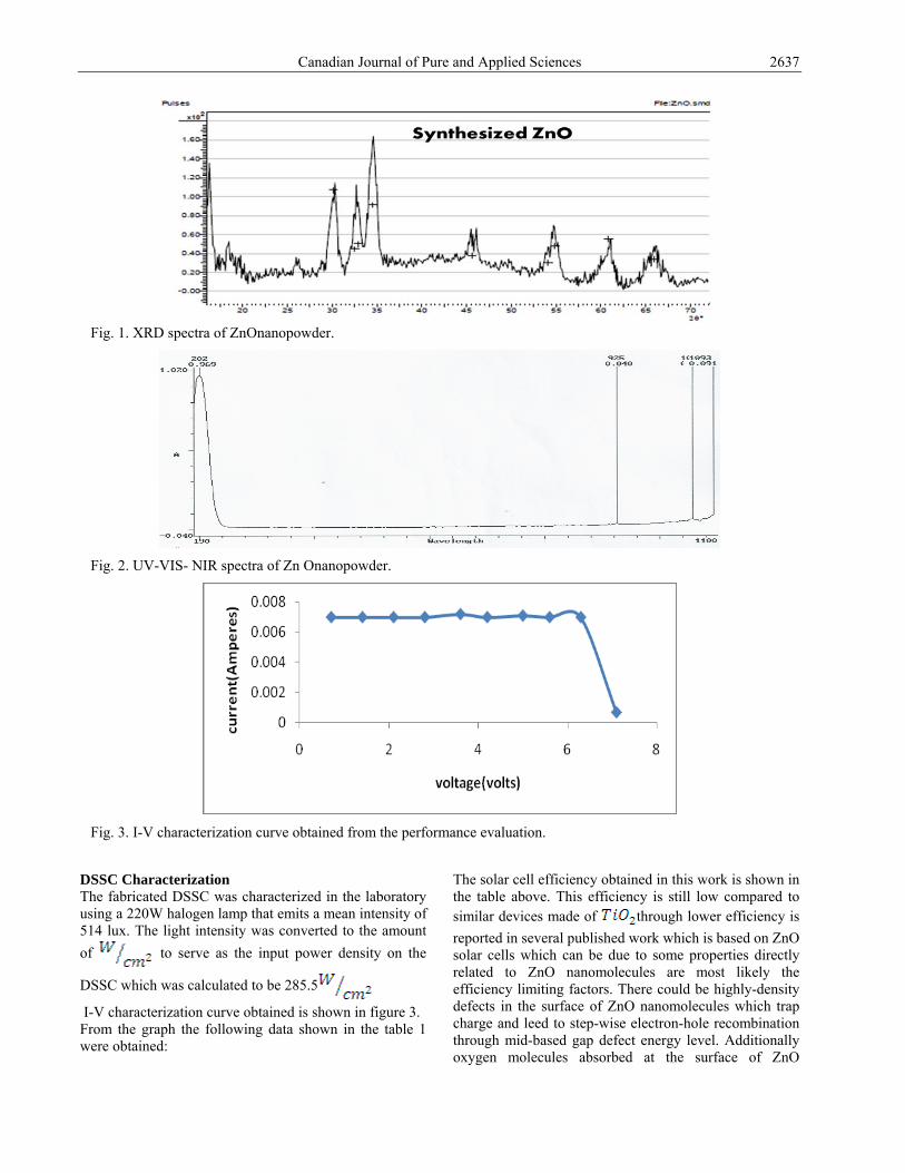
Canadian Journal of Pure and Applied Sciences 2637
DSSC Characterization The fabricated DSSC was characterized in the laboratory using a 220W halogen lamp that emits a mean intensity of 514 lux. The light intensity was converted to the amount of to serve as the input power density on the
DSSC which was calculated to be 285.5
I-V characterization curve obtained is shown in figure 3. From the graph the following data shown in the table 1 were obtained:
The solar cell efficiency obtained in this work is shown in the table above. This efficiency is still low compared to similar devices made of through lower efficiency is reported in several published work which is based on ZnO solar cells which can be due to some properties directly related to ZnO nanomolecules are most likely the efficiency limiting factors. There could be highly-density defects in the surface of ZnO nanomolecules which trap charge and leed to step-wise electron-hole recombination through mid-based gap defect energy level. Additionally oxygen molecules absorbed at the surface of ZnO
Fig. 1. XRD spectra of ZnOnanopowder.
Fig. 2. UV-VIS- NIR spectra of Zn Onanopowder.
Fig. 3. I-V characterization curve obtained from the performance evaluation.

Oladiran and Olabisi 2638
nanomolecules can serve as efficient excitation quenching centre (Tao et al., 2011). CONCLUSION ZnO nanoparticles synthesized by precipitating Zinc nitrate hexahydrate has been used in the fabrication of DSSC using Eosin blue as the sensitizer with lemon juice as the electrolyte and for the first time using metal contact on a nonconductive glass as electrode from the performance evaluation the ZnO with crystal size of 26.04nm was used to obtain an efficiency of 0.15% which has made this new dimension successful and a new foundation for easy research in the world of photovoltaic in developing countries. REFERENCES Abel, OF., Gil Nonato Santos, C. and Reuben, QV. 2012. Fabrication and characterization of dye sensitized solar cell using nanostructured TiOPhotoelectrode. International Journal of Science and Engineering Research. 3:554-559.
Aydil, E. 2007. Nanomaterials for solar cells. Nanotechnology Law and Business. 4(3):275-291.
Bach, ULD., Comte, PM Je., Wiessortel, F., Salbeck, H. and Gratzel, M. 1998. Solid state dye-sensitized mesoporous TiO2 solar cell with high photo-to-electron conversionefficiencies. Nature. 395:583-585.
Brian, EH., Henry, JS. and Michael, DM. 2012. The renaissance of dye-sensitized solar cells. Nature Photonics. 6. doi:10.1038/NPHOTON.2012.22
Gratzel, M. 2003. Dye-sensitized solar cells. Journal of photochemical and Photobiology C: photochemistry. doi: 10.1016/s1389-5567(03)00026-1
Monishka, RN. 2012. Dye Sensitized Solar cells based on natural photosensitized Renewable and Sustainable Energy Reviews. doi: 10.1016/j.rser.2011.07.143
O’Regan, B. And Gratzel, M. 1991.A low cost, high-efficiency solar cell based on dye sensitized colloidal TiO2 films. Nature. 353:737-739.
Tao-Hua, Lee., Hung-Jue, Sue. and Xing Cheng. 2011. Solid-state dye-sensitized solar cells based on ZnO nanoparticles and nanorod array hybrid photoanodes. Nanoscale research letters. doi:10.1186/1556-276X-6.517.
Yu, K. and Chen, J. 2009. Enhancing solar cell efficiencies through 1-D nanostructures. Nanoscale Research letter. 4:1-10.
Received: Feb 23, 2013; Accepted: June 5, 2013
Table 1. Evaluation parameters obtained from the DSSC.
(V) (A) (V) 0.0070 7.1000 0.0712 7.3000 0.855 0.15%

SENRA Academic Publishers, British Columbia Vol. 7, No. 3, pp. 2639-2647, October 2013 Online ISSN: 1920-3853; Print ISSN: 1715-9997 Short Communication
AN-VE: AN IMPROVED HAMMING CODING TECHNIQUE
*Egwali Annie O and Akwukwuma V V N
Department of Computer Science, Faculty of Physical Sciences University of Benin, PMB. 1154, Benin City, Nigeria
ABSTRACT
Many communication channels are subject to noise, and thus errors may be introduced during transmission. Error codes can be units of deliberate error injection or faults, which alters and cause hazards during communication, this makes error detection and correction important in the computing environment. Coding techniques restricted to detecting errors only are either limited to analyzing only the length of the encoded message bits or repeats every transmitted stream of bit(s) several times in order to check for correctness, which is not effective if similar error occurs within the same position on all clusters of bits in the encoded message. Error detecting and correcting techniques are more thorough by introducing extra redundant codes to detect the actual position of errors and correcting them, however if more than one error occurs, it becomes difficult to detect all errors and decode correctly. We therefore propose a hybrid error detecting and correcting technique, AN-VE, that simultaneously detect the existence of faulted codes right from the transmitter domain, analyzes all error positions in the encoded message via the use of extra parity bits, decode all errors correctly and verify error messages with the original message. We evaluate our approach using simulated and real data. Keywords: Error, code, parity, hamming, parity. INTRODUCTION As present society relies on the fault-free operation of computing systems, system fault-tolerance has become a serious issue that needs addressing. Common agreement exists that large cluster of system codes always contain faults and thus precautions must be taken to avoid system failure. Failure of generated and transmitted codes often can be caused by external or internal factors that can or cannot be avoided, predicted, or corrected. Therefore, techniques are needed that guarantee correct data representation and transmission in the presence of errors (Kahn, 1996). To enable reliable delivery of digital data over reliable or unreliable communication channels, digital code redundancy techniques have been classified into two basic types: error detecting code technique and error detecting and correcting code technique. Error detecting technique is most commonly realized using a suitable hash function that adds a fixed-length tag to a message, and facilitates receivers to verify the delivered message by re-computing the tag and comparing it with the one provided. The enormous variety of dissimilar hash function designs is because of their simplicity or their suitability for detecting errors of different kinds. Error detecting and correcting code technique have the ability to detect, locate and correct errors. Consequently any error correcting code can be used for error detection.
Coding techniques restricted to detecting errors only are either limited to analyzing just the length of the encoded message bits without specifying the actual bits with errors, or every transmitted stream of bit(s) is repeated several times in order to check for correctness, which does not prove effective if similar error occurs within the same position on all clusters of bits in the encoded message. In order for a system to deliver its expected service in the presence of errors caused by faults or units of deliberate error injection, some extra redundant codes are needed. Redundancy involves the inclusion of some extra codes in order to check the correctness or the consistencies of the results produce, and if the need arises, concurrent computations are chosen. Also the effects of faults can be masked with no specific indication of their occurrence, thus error effects are hidden from the rest of the system. In addition, faulty codes can be removed or replace in response to system failure, a process usually triggered either by internal error detection mechanisms in the faulty coded unit(s) of the software or by detection of errors in the output(s) of these units. These redundant codes are evident in some error detecting and correcting techniques, which makes them more thorough, because it helps to detect the actual position of the errors and correct the errors. Nevertheless, if more than one error occurs in an encoded stream message bit, error detecting and correcting techniques have difficulties in detecting all errors and decoding them correctly. Codes fault tolerance is very necessary, but can itself be dangerously error-prone because of the additional effort that must be *Corresponding author email: [email protected]

Egwali and Akwukwuma 2640
involved in the programming process. The additional redundancy may increase size and complexity and thus adversely affect information, software and by extension hardware reliability. Fletcher (1982) developed a Checksum algorithm that involves detecting errors commonly introduced by humans in writing down or remembering identification numbers (Stallings, 2003). The checksum of a message is a modular arithmetic sum of a stream of message bits (SMB) of a fixed length, which could be negated by means of a one's-complement prior to transmission to detect errors resulting in all-zero messages (Fletcher, 1982). In repetition code technique, involves error detection, every transmitted stream of bit(s) is repeated several times in order to check for correctness (Filiol, 2003; Courtois, 2002). Unfortunately, repetition codes prove not to be effective if similar error occurs within the same position on all clusters of bits in the stream. Berger (1961) developed the Berger code which can detect all unidirectional errors, that is errors that only flip ones into zeroes or only zeroes into ones, such as in asymmetric channels. The check bits of Berger codes are computed by summing all the zeroes in the stream of message bits, and expressing that sum in natural binary. Berger codes can detect any number of one-to-zero bit-flip errors, as long as no zero-to-one errors occurred in the same stream of message bits. Berger codes can detect any number of zero-to-one bit-flip errors, as long as no one-to-zero bit-flip errors occur in the same SMB but cannot correct any error (Wiki, 2009). Hamming (1969) posited the hamming error and correcting coding technique which are the earliest linear error correcting code technique. It involves the use of an extra parity bit to ensure the identification of a single error. However, if more than one error occurs, the Hamming Decoder block decodes incorrectly. Peterson (1960) proposed parity coding technique, which can only detect single errors and any odd number of errors. In this technique extra bits are added to the source bits so that the derived bits with value 1 in the set of bits are either even or odd (Peterson and Brown, 1961). When using even parity, the parity bit is set to 1 if the number of ones in a given set of bits (not including the parity bit) is odd, making the entire set of bits (including the parity bit) even. When using odd parity, the parity bit is set to 1 if the number of ones in a given set of bits (not including the parity bit) is even, keeping the entire set of bits (including the parity bit) odd. In other words, an even parity bit will be set to "1" if the number of 1's + 1 is even, and an odd parity bit will be set to "1" if the number of 1's +1 is odd (Wiki, 2010). This coding technique is applicable in data storage and retrieval from or into the computer memory. A shortfall with this technique is that for an odd flipped bit codes, an erroneous code with an odd flipped bit will be assumed to be correct. Also parity coding technique
can only detect single errors and any odd number of errors. According to Wiki (2010a), parity does not indicate which bit contained the error, even when it can detect it. The data must be discarded entirely and re-transmitted from scratch. On a noisy transmission medium, a successful transmission could take a long time or may never occur. Borden codes denoted as Bi/j are a set of codes of length j for which exactly i bits are ones. The union of codes with i being the set of values congruent to
is the Borden (j, k) code. For example, to derive the Borden (7, 3) code, by substituting values for j and k, we will have:
. Hence i belong to the set 0, 3, 6. This means that source codes of length 7 (e.g. 0000000, 0011100, 0101010, 0111111, 1111011), which have no bits, three bits or six bits of digit 1 belongs to the Borden code set. A shortfall with this technique is that although the Borden (j, k) can detect k unidirectional errors (e.g. an erroneous conversion of 0 to 1 or 1 to 0), it cannot detect both erroneous conversion at the same time. MATERIALS AND METHODS A hybrid model called AN-VE that incorporates the unique features inherent in the cyclic redundancy checking (CRC) technique and the Hamming error detecting and correcting (HEDC) technique was proposed. AN-VE offers a more robust error detecting and correcting mechanism right from the transmitter domain, unlike repetition coding technique, which is not effective at detecting errors if similar error occurs within the same position on all clusters of bits in the encoded message bit stream. AN-VE is also more efficient than the CRC technique at detecting errors, which only analyzes the length of the encoded message bits against the initial message bits because it both verify the length of the encoded message and addresses all error positions via the use of extra parity bits. AN-VE also performs better that the HEDC technique, which is not able to detect all errors accurately if more than one error occurs in a decoded stream of message bits. AN-VE decodes and corrects all errors correctly and verifies decoded error messages with the original message. We evaluate our approach using simulated and real data. AN-VE Error Detecting and Correcting Method AN-VE (f, g) code like the hamming code consists of “g” data bits and the encoded data bits of length f. g is defined by the equation: g = 2a – a − 1, and f is defined by the equation, f = 2a − 1, were “a” denotes the parity bits such that a 3. AN-VE is a technique that offers a more robust error detecting and correcting mechanism. Correcting and detecting error codes involves the following three phases.

Canadian Journal of Pure and Applied Sciences 2641
Phase One: Creation of Message Bits This phase executes the four steps process of the Hamming coding technique to create a stream of message bits. For example, for the following stream of message bits: 11010011101100 Step 1 and Step 2 yields: _ _1_101-
_0011101_100 Step 3 and Step 4: Using * to denote the parity bit
position, the following results are derived for each position:
Position 1 yields: * _1_101_0011101_100 This is an even parity hence position 1 is set to 0: 0_1_101_0011101_100
• Position 2 yields: 0*1_101_0011101_100 This is an even parity hence position 2 is set to 0: 001_101_0011101_100
Position 4 yields: 001*101_0011101_100 This is an odd parity hence position 4 is set to 1: 0011101_0011101_100
Position 8 yields: 0011101*0011101_100 This is an even parity hence position 8 is set to 0: 001110100011101_100
Position 16 yields: 001110100011101*100 This is an odd parity hence position 16 is set to 1: 0011101000111011100
Consequently, the expected created SMB is 0011101-000111011100. Phase Two: Error Verification After the initial phase, if the created SMB is suppose to be 0011101000111011100, but due to noise the message bits received is 0011111000101011110, the system is able to detect this error because the second phase of AN-VE checks each inputted bit in the received SMB for accidental changes. During this stage, the system first check the length of the input code bits received for changes (see Tables 1 and 2) by lining input bits in a row, and a (n+1)-bit pattern that acts as a Cyclic redundancy
Table 1. AN-VE Error Detecting Method (created and received SMB are equivalent).
Created SMB: 0 0 1 1 1 0 1 0 0 0 1 1 1 0 1 1 1 0 0 Divisor 1 0 1 1 Received SMB: 0 0 1 1 1 0 1 0 0 0 1 1 1 0 1 1 1 0 0 Divisor 1 0 1 1 Received SMB: 0 0 1 1 1 0 1 0 0 0 1 1 1 0 1 1 1 0 0 Divisor 1 0 1 1 Received SMB: 0 0 0 1 0 1 1 0 0 0 1 1 1 0 1 1 1 0 0 Divisor 1 0 1 1 Received SMB: 0 0 0 0 0 0 0 0 0 0 1 1 1 0 1 1 1 0 0 Divisor 1 0 1 1 Received SMB: 0 0 0 0 0 0 0 0 0 0 1 1 1 0 1 1 1 0 0 Divisor 1 0 1 1 Received SMB: 0 0 0 0 0 0 0 0 0 0 1 1 1 0 1 1 1 0 0 Divisor 1 0 1 1 Received SMB: 0 0 0 0 0 0 0 0 0 0 1 1 1 0 1 1 1 0 0 Divisor 1 0 1 1 Received SMB: 0 0 0 0 0 0 0 0 0 0 1 1 1 0 1 1 1 0 0 Divisor 1 0 1 1 Received SMB: 0 0 0 0 0 0 0 0 0 0 1 1 1 0 1 1 1 0 0 Divisor 1 0 1 1 Received SMB: 0 0 0 0 0 0 0 0 0 0 1 1 1 0 1 1 1 0 0 Divisor 1 0 1 1 Received SMB: 0 0 0 0 0 0 0 0 0 0 0 1 0 1 1 1 1 0 0 Divisor 1 0 1 1 Received SMB: 0 0 0 0 0 0 0 0 0 0 0 0 0 0 0 1 1 0 0 Divisor 1 0 1 1 Received SMB: 0 0 0 0 0 0 0 0 0 0 0 0 0 0 0 1 1 0 0 Divisor 1 0 1 1 Received SMB: 0 0 0 0 0 0 0 0 0 0 0 0 0 0 0 1 1 0 0 Divisor 1 0 1 1 Received SMB: 0 0 0 0 0 0 0 0 0 0 0 0 0 0 0 1 1 0 0 Divisor 1 0 1 1 Result 0 0 0 0 0 0 0 0 0 0 0 0 0 0 0 0 1 1 1

Egwali and Akwukwuma 2642
check divisor is positioned underneath the left-hand end of the row. If the input bit above the leftmost divisor bit is 0, the bit is left and the divisor is moved to the right by one bit. If the input bit above the leftmost divisor bit is 1, the divisor is XORed into the input. The divisor is then shifted one bit to the right, and the process is repeated until the divisor reaches the right-hand end of the input row. Since the leftmost divisor bit zeroed every input bit it touched, when this process ends the only bits in the input row that can be nonzero are the n bits at the right-hand end of the row, which will always be less than the divisor.
Phase Three: Error Correction After checking for changes, if the created SMB does not match the received SMB (i.e. the system reads “0000000000000001000” gotten from the received SMB “0011111000101011110” instead of “0000000000000000111” from the created SMB “0011101000111011100”), AN-VE established that the received code block contains data error and take corrective measures to detect the actual bit locations containing the errors. The affected check bits positions are established, which are positions 2 check bit and 4 check bit for error bit at position 6 of received SMB;
Table 2. AN-VE Error Detecting Method (Created and Received SMB are not equivalent).
Created SMB: 0 0 1 1 1 0 1 0 0 0 1 1 1 0 1 1 1 0 0 Received SMB: 0 0 1 1 1 1 1 0 0 0 1 0 1 0 1 1 1 1 0 Divisor 1 0 1 1 Received SMB: 0 0 1 1 1 1 1 0 0 0 1 0 1 0 1 1 1 1 0 Divisor 1 0 1 1 Received SMB: 0 0 1 1 1 1 1 0 0 0 1 0 1 0 1 1 1 1 0 Divisor 1 0 1 1 Received SMB: 0 0 0 1 0 0 1 0 0 0 1 0 1 0 1 1 1 1 0 Divisor 1 0 1 1 Received SMB: 0 0 0 0 0 1 0 0 0 0 1 0 1 0 1 1 1 1 0 Divisor 1 0 1 1 Received SMB: 0 0 0 0 0 1 0 0 0 0 1 0 1 0 1 1 1 1 0 Divisor 1 0 1 1 Received SMB: 0 0 0 0 0 0 0 1 1 0 1 0 1 0 1 1 1 1 0 Divisor 1 0 1 1 Received SMB: 0 0 0 0 0 0 0 1 1 0 1 0 1 0 1 1 1 1 0 Divisor 1 0 1 1 Received SMB: 0 0 0 0 0 0 0 0 1 1 0 0 1 0 1 1 1 1 0 Divisor 1 0 1 1 Received SMB: 0 0 0 0 0 0 0 0 0 1 1 1 1 0 1 1 1 1 0 Divisor 1 0 1 1 Received SMB: 0 0 0 0 0 0 0 0 0 0 1 0 0 0 1 1 1 1 0 Divisor 1 0 1 1 Received SMB: 0 0 0 0 0 0 0 0 0 0 0 0 1 1 1 1 1 0 0 Divisor 1 0 1 1 Received SMB: 0 0 0 0 0 0 0 0 0 0 0 0 1 1 1 1 1 0 0 Divisor 1 0 1 1 Received SMB: 0 0 0 0 0 0 0 0 0 0 0 0 0 1 0 0 1 0 0 Divisor 1 0 1 1 Received SMB: 0 0 0 0 0 0 0 0 0 0 0 0 0 0 0 1 0 0 0 Divisor 1 0 1 1 Received SMB: 0 0 0 0 0 0 0 0 0 0 0 0 0 0 0 1 0 0 0 Divisor 1 0 1 1 Result 0 0 0 0 0 0 0 0 0 0 0 0 0 0 0 1 0 0 0

Canadian Journal of Pure and Applied Sciences 2643
positions 4 check bit and 8 check bit for error bit at position 12 of received SMB; positions 2 check bit and 16 check bit for error bit at position 16 of received SMB. To effectively correct all errors, unlike the conventional hamming technique that can only handle one error correction in a SMB, AN-VE devices a parsing procedure that parses each n-bit binary position on the received SMB which are lined in a row and compares it with the n-bit binary position of the created SMB which are lined in a row starting from the extreme left. The parity check bits of the first bit at variance between the two sets of n-bit binary position in a row are verified to detect the error, which is then, corrected using the hamming error correcting and at each parsing stage, the system only
acknowledges the positions of the other bits in the row and not their values. The system repeats this process till all n-bit binary positions is parsed and both created and received codes are equivalent (see Table 3). EXPERIMENT To demonstrate the efficiency of AN-VE over HEDC in detecting and correcting errors during communication, we analytically simulate the performance of the techniques in the presence of error in form of noise in a channel of communication using simulink that runs in Matlab. Generally in every communication system the basic components of communication are the original data bits,
Table 3. AN-VE Corrective Mechanism.
Created SMB: 0 0 1 1 1 0 1 0 0 0 1 1 1 0 1 1 1 0 0 Received SMB: 0 0 1 1 1 1 1 0 0 0 1 0 1 0 1 1 1 1 0 AN-VE Parsing: _ _ _ _ _ _ _ _ _ _ _ _ _ _ _ _ _ * 0 HEDC Correction: _ _ _ _ _ _ _ _ _ _ _ _ _ _ _ _ _ 0 0 Created SMB: 0 0 1 1 1 0 1 0 0 0 1 1 1 0 1 1 1 0 0 Received SMB: 0 0 1 1 1 1 1 0 0 0 1 0 1 0 1 1 1 0 0 AN-VE Parsing: _ _ _ _ _ _ _ _ _ _ _ * 1 0 1 1 1 0 0 HEDC Correction: _ _ _ _ _ _ _ _ _ _ _ 1 1 0 1 1 1 0 0 Created SMB: 0 0 1 1 1 0 1 0 0 0 1 1 1 0 1 1 1 0 0 Received SMB: 0 0 1 1 1 1 1 0 0 0 1 1 1 0 1 1 1 0 0 AN-VE Parsing: _ _ _ _ _ * 1 0 0 0 1 1 1 0 1 1 1 0 0 HEDC Correction: _ _ _ _ _ 0 1 0 0 0 1 1 1 0 1 1 1 0 0 Created SMB: 0 0 1 1 1 0 1 0 0 0 1 1 1 0 1 1 1 0 0 Received SMB: 0 0 1 1 1 0 1 0 0 0 1 1 1 0 1 1 1 0 0
Fig. 1. Hamming Encoder.
Fig. 2. Simulink of the HEDC Communication Components.
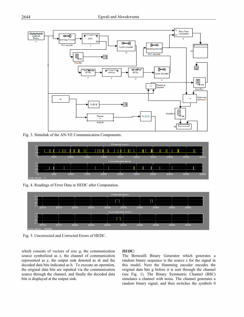
Egwali and Akwukwuma 2644
which consists of vectors of size g, the communication source symbolized as x, the channel of communication represented as y, the output sink denoted as sk and the decoded data bits indicated as b. To execute an operation, the original data bits are inputted via the communication source through the channel, and finally the decoded data bits is displayed at the output sink.
HEDC: The Bernoulli Binary Generator which generates a random binary sequence is the source x for the signal in this model. Next the Hamming encoder encodes the original data bits g before it is sent through the channel (see Fig. 1). The Binary Symmetric Channel (BSC) simulates a channel with noise. The channel generates a random binary signal, and then switches the symbols 0
Fig. 3. Simulink of the AN-VE Communication Components.
Fig. 4. Readings of Error Data in HEDC after Computation.
Fig. 5. Uncorrected and Corrected Errors of HEDC.

Canadian Journal of Pure and Applied Sciences 2645
and 1 or the reverse in the signal, according to a specified error probability, to simulate a channel with noise.
The Hamming decoder decodes the data after it is sent through the channel. It verifies if an error is created in the original data bits by the noise in the channel, identifies the error and decodes the data received to the original data bits correctly. The bits error rate represented as err is computed at z, which in this case detects and computes the error rate of the channel using the values of its two input ports, the transmitted signal Tx and the received signal Rx. The computation is based on the following
equation (1), which denotes the probability of two or more errors occurring in encoded data bits of length f. err = 1 – (0.99)f – f(0.99)f-1(0.01) (1)
The bits error rate result is displayed in the first box of sk after the termination of execution. The second box of sk displays the number of errors occurrences. The third box of sk displays the total number of bits (bn) transmitted. The logical inference and relationship between the components are represented in figure 2, which contains a sample of the readings of HEDC [(1023, 1013)].
Fig. 6. Readings of Error Data (AN-VE) After Computation.
Table 4. Computational Readings.
Bits error rate (err) Number of errors Transmitted bits
Encoded data bits length
(f)
Data bits (g)
Parity bits (s) HEDC AN-VE HEDC AN-VE
9.474e+004 7 4 3 0.001066 0.0057 101 54 5.007e+004 15 11 4 0.001997 0.0002397 100 12 2.415e+004 31 26 5 0.00414 0.000207 100 5 1.664e+004 63 57 6 0.006068 0.000201 101 4 1.02e+004 127 120 7 0.0101 0.00103 103 2 8151 255 247 8 0.01227 0.00114 100 9 9036 511 502 9 0.01162 0.001771 105 16 1.013e+004 1023 1013 10 0.01076 0.001382 109 14 1.018e+004 2047 2036 11 0.01041 0.001081 106 11
020406080100120
Num
ber o
f Error
Transmitted bits
HEDC
AN‐VE
Fig. 7. Available Errors in Transmitted Bits after Applying HEDC and AN-VE Techniques.

Egwali and Akwukwuma 2646
AN-VE: For AN-VE, the source x is the Bernoulli Binary Generator. Next the Hamming encoder encodes the original stream of message bits g before it is sent through the Binary Symmetric Channel (BSC) that adds binary errors to the input signal (see Fig. 3). The cyclic encoder creates the systematic cyclic bits with message length K and encoded SMB length N in the binary cyclic encoder. The code rate is:
Code rate = ge/fe = message bits length/ encoded SMB length
where ge is the message length and fe is the length of the derived encoded data bits and “a” denotes the check bits such that ge = 2a − a − 1, fe = 2a − 1, a 3. Then the input SMB is modulated using the binary phase shift keying (BPSK) method, which is a technique for modulating a binary signal onto a complex waveform by shifting the phase of the complex signal. In digital baseband BPSK, the symbols 0 and 1 are modulated to the complex numbers exp(t) and -exp(t), respectively, where t is a fixed angle. Thus for t = 0, these numbers are just 1 and -1. The AWGN channel add white Gaussian noise to the input codes and it is more robust than the binary symmetric channel in some specific applications because it accepts both real or complex codes and it supports multichannel input and output codes inputs as well as frame-based processing. The Hamming decoder parses through the n-bit binary position on the received SMB bits and decodes the data after it is sent through the channel. It verifies if an error is created in the original data bits by the noise in the channel, identifies the error and decodes the data received to the original data bits correctly. The system repeats this process till all n-bit binary positions is parsed and both transmitted and received codes are equivalent. After each AN-VE Parsing, the bits error rate (err) of the created SMB and received SMB is computed at z, which detects and computes the error rate of the channel using the values of the transmitted signal Tx and the received signal Rx ports. The block compares the two signals and checks for errors. The output depicted as sk is a vector with three entries: bit error rate, number of errors and total number of bits transmitted. RESULTS AND DISCUSSION The readings of the upper section of figure 4 reveal the channel of uncorrected errors in an encoded SMB generated by the channel coding of HEDC, which are pulses represented as 1s. The readings of the lower section of figure 4 shows the same encoded SMB but with fewer errors at the end of each 5000 time steps. A proximity assessment of upper section of figure 4 shows that in the single encoded SMB, two 1s represented as the wider rectangular pulse, are errors not corrected,
whereas the narrower rectangular pulse to the right of the upper section represents a single error, which is corrected (see Fig. 5). The two 1s, which are uncorrected, accounts for the uncorrected errors in the lower section. Figure 6 shows the performance of AN-VE with the upper and lower sections of the figure revealing the channel of uncorrected and corrected errors respectively. It is evident that with the same number of bits transmitted (see Table 4), AN-VE performed better, for the two 1s which are uncorrected, are far less than is the case with HEDC, this is also shown in figure 7, which reveals the number errors left over in the transmitted bits after the application of both techniques. CONCLUSION Fault tolerance solutions can be implemented using various methodologies. Each method has its own tradeoffs in terms of strength in detecting errors, potency in correcting errors, portability, and ease of use. We proposed a detecting and correcting technique that is more robust than HEDC because although HEDC is quite useful in cases where only a single error is of significant probability, the technique can only be used to detect up to two simultaneous bit errors and correct single errors, both cannot be done simultaneously. Also because the technique can only correct one error in each transmitted stream of message bits, if more than one error occurs, the Hamming decoder does carry the hazard of miscorrecting double errors. Conversely, AN-VE enables the detection of any number of simultaneous bit errors and corrects all errors and both can be done simultaneously. Furthermore unlike the HEDC which deals with error detection after data transmission, AN-VE addresses error detection right from the transmitter domain. AN-VE can detect the erroneous bit in a transmitted code because every transmitted code is repeated several times in order to verify its accuracy. REFERENCES Berger, JM. 1961. A note on an error detection code for asymmetric channels. Information and Control. 4: 68-73.
Courtois, NT. 2002. Cryptanalysis of block ciphers with overdefined systems of equations. Advances in Cryptology – AsiaCrypt 2002, Lecture Notes in Computer Science 2501, Springer-Verlag. 267-287, doi:10.1007/3-540-36178-2_17.
Filiol, E. 2003. Plaintext-dependent Repetition Codes Cryptanalysis of Block Ciphers - the AES Case, Published on eprint on 8th of January 2003. Available at: http://eprint.iacr.org/2003/003
Fletcher, JG. 1982. An Arithmetic Checksum for Serial Transmissions. IEEE Trans. on Comm. 30(1): 247-252.

Canadian Journal of Pure and Applied Sciences 2647
Hamming, RW. 1980. The Unreasonable Effectiveness of Mathematics. The American Mathematical Monthly. 87:81-90.
Hamming, RW. 1969. One Man's View of Computer Science. Journal of the ACM. 16 (1):3-12.
Kahn, D. 1996. The Codebreakers: The Story of Secret Writing, New York: Macmillan Publishing Co., 1967. Available at: http://www.cse.iitk.ac.in/users/anuag/crypto.pdf. Nicolas, T. 2003. Did Filiol Break AES?, Published on e-print on 4th of February 2003. Available at: http://eprint.iacr.org/2003/022.
Peterson, WW. 1960. Encoding and Error-Correction Procedures for the Bose-Chaudhuri Codes. IRE Transactions on Information Theory. IT-6:459-470.
Peterson, WW. and Brown, DT. 1961. Cyclic Codes for Error Detection. Proceedings of the IRE. 49:228. doi:10.1109/JRPROC.1961.287814.
Stallings, W. 2003. The TCP/IP Checksum. Available at: http://tchandouts.com/07315/Checksum.pdf
Wiki 2010. Parity Bit. Available at: http://en.wikipedia.org/wiki/Parity_bit.
Wiki 2010a. Hamming Code. Available at: http://en.wikipedia.org/wiki/Hamming_code.
Received: March 20, 2013; Accepted: Aug 12, 2013

SENRA Academic Publishers, British Columbia Vol. 7, No. 3, pp. 2649-2653, October 2013 Online ISSN: 1920-3853; Print ISSN: 1715-9997 Short communication
PREDICTIVE MODELS ON SETTLEMENT PARAMETERS OF CLAYEY SOILS:
A CASE STUDY IN PORT-HARCOURT CITY OF NIGERIA
S B Akpila Department of Civil Engineering, Rivers State University of Science and Technology
P.M.B 5080, Port Harcourt, Nigeria
ABSTRACT Settlement parameters of shallow foundations placed on clayey soils have been studied in PortHarcourt City of Nigeria. Fifty soil samples were obtained from six locations and subsequently subjected to oedometer tests. Settlement parameters of void ratio,e, coefficient of volume compressibility, mv, and compression modulus, Ec, were deduced from oedometer results. Results of e, and mv generally showed a decreasing trend with increase in pressure, while Ec increases with pressure. Predictive models relating void ratio and pressure, coefficient of volume compressibility and pressure, and that of compression modulus and pressure, were subsequently formulated. The generated models can be used for quick evaluation of settlement input parameters required in settlement analysis of foundation placed on cohesive soil formation. Keywords: Void ratio, compression modulus, volume compressibility, foundation. INTRODUCTION The deformation tendency of foundation placed on saturated cohesive soils is time dependent. Usually, both immediate and consolidation settlement are assessed to determine if the expected deformation is within the tolerance limit of the superstructure. Details on limiting settlement criteria for shallow foundations placed on either cohesive or granular soils have been presented by scholars (Polshin and Tokar, 1957; Wahls, 1981; Skempton and McDonald, 1956, Murthy, 2007). Evaluation of immediate settlement of shallow foundation placed on cohesive soils requires knowledge of the undrained modulus, Eu, of the supporting soil. However, determination of Eu is faced with several challenges. Barnes (2000) and Jamiolkowski et al. (1979) proposed ratio of undrained modulus to undrained cohesion (Eu/cu) depending on over consolidation ratio and plasticity index. Butler (1974) proposed Eu/cu ratio of 400 for over consolidated London clay, while Bjerrum (1973) proposed cu/p ratios in the range of 500 to 1500 for normally consolidated clays. Smith (1984) reported Skempton (1951) to have presented a procedure of obtaining undrained modulus directly from triaxial test results by determining the strain corresponding to 65% of the maximum deviator stress and dividing this value to the corresponding stress. In many literatures, Eu for various soils is presented in a wide range of values (Bowles, 1997).
In consolidation settlement, soil parameters such as void ratio, e, and coefficient of volume compressibility, mv, of the compressible soil formation that is significantly affected by the foundation induced vertical stress are required. The void ratio of a soil expresses the ratio of volume of void to volume of solid (Barnes, 2000), while coefficient of volume compressibility is the compression of a soil layer per unit of original thickness due to a given unit increase in pressure (Raj, 2008).The reciprocal of mv is compression modulus, Ec, and is analogous to Youngs modulus (Garg, 1987). In Tomlinson (2001), the various range of coefficient of volume compressibility of soils is given and usually, the settlement parameters are derived from results of oedometer test with details of test procedure in BS 1377. Based on the difficulty in evaluating the relevant settlement parameters required in computing foundation settlement, an attempt is made in this paper to develop predictive models in the study area to aide preliminary analysis and design of shallow foundations placed on clayey soils. MATERIALS AND METHODS Data Aquisition / Analysis A total of fifty soil samples were obtained from borings to depth of 5m at six different areas of PortHarcourt; Eagle Island, Agip, East West Road, Abuloma, Rumuigbo, and PortHarcourt Town. Soil samples were subjected to oedometer test from which void ratio and coefficient of volume compressibility of each soil sample were
*Corresponding author email: [email protected]

Akpila 2650
evaluated using the following equations (Smith, 1984; Raj, 2008).
(1)
(2)
Where H1 is thickness at the end of any increment period, Ms is mass of sample measured at the end of test, A is area of specimen, G is specific gravity of soil sample, ρw is density of water, e1 is void ratio corresponding to pressure p1, e0 is void ratio corresponding to pressure po, mv is coefficient of volume compressibility, ∆e and ∆p are change in void ratio and pressure respectively. The average values of void ratios and coefficient of volume compressibility of soil samples were obtained for varying pressure range on each study area. Subsequently, the following relationships were evaluated; void ratio versus pressure, coefficient of volume compressibility versus pressure and reciprocal of coefficient of volume compressibility versus pressure. RESULTS AND DISCUSSION Void Ratio and Pressure Variation The variation of void ratio and pressure is depicted in figure 1. Here, the trend lines are closely related, depicting a gradual decrease in void ratio (e) as pressure increases for Rumuigbo, Agip, Eagle Island, East West Road and Port Harcourt Town. Values of void ratio ranged between 0.80-0.40 for pressure range of 0-
800kN/m2 respectively in these five areas and mv values are indicative of medium compressibility soils. In Abuloma, the soils also had a gradual decrease in void ratio as pressure increased but higher e values are associated with this area. The model equations expressing variation of void ratio versus pressure for each study area are given as follows: Abuloma: e = -3E-09p3+4E-06p2-0.002p+1.444; R2=0.996 (3) East West Road: e = -5E-10p3+9E-07p2+0.737; R2=0.999 (4) Rumuigbo: e = -5E-10p3+9E-07p2+0.737; R2=0.999 (5) PortHarcourt Town: e = 2E-07p2+0.617; R2=0.981 (6) Eagle Island: e = -7E-10p3+1E-06p2+0.583; R2=0.998 (7) Agip: e = -7E-07p2+0.617; R2=0.981 (8) Coefficient of Volume Compressibility and Pressure Variation In figure 2, the variation of coefficient of volume compressibility and pressure is shown. The trend lines showed a rapid decrease in mv through a pressure range of 0-100kN/m2, beyond which mv had a gradual decrease as pressure increased. The Abuloma area had higher values of mv compared to the other five areas of study, for any pressure range. At pressures exceeding 100kN/m2, the compressibility characteristics of soils within Rumuigbo, Agip, East West Road, Eagle Island and Port Harcourt Town areas showed very close approximation. Generally, mv values are indicative of medium compressibility soils.
Fig. 1. Variation of void ratio versus pressure.

Canadian Journal of Pure and Applied Sciences
2651
The predictive models relating coefficient of volume compressibility and pressure are presented in Equations (9-14). Eagle Island: mv= -1E-08p3 + 1E-05p2 - 0.0035p + 0.4444 (9) Rumuigbo: mv= -1E-08p3 + 9E-06p2 - 0.0023p + 0.3197 (10) Agip: mv = -2E-08p3 + 2E-05p2 – 0.0051p + 0.5682 (11) Abuloma: mv = -3E-08p3 + 3E-05p2 - 0.008p + 0.9997 (12) East West Road: mv = 2E-06p2
- 0.0016p + 0.3461 (13) Port Harcourt Town: mv= -2E-08p3 + 1E-05p2
- 0.0039p + 0.4235 (14) Compression modulus versus Pressure The variation of compression modulus, Ec, and pressure is depicted in figure 3, where Ec increased with pressure and the values are easily predictable at pressures exceeding 100kN/m2. Soils from PortHarcourt town exhibited the highest values of compression modulus while Abuloma area had lowest values at pressures exceeding 100kN/m2. The predictive models relating compression modulus and pressure in the six areas are presented in Equations (15-20) as follows: Eagle Island: 1/mv = 7E-06p2 + 0.031p
Fig. 2. Variation of coefficient of volume compressibility versus Pressure.
Fig. 3. Variation of Compression modulus versus Pressure.

Akpila 2652
+ 2.039, R2 = 0.997 (15) Rumuigbo: 1/mv = 1E-07p3 - 6E-05p2 + 0.034p + 3.044, R2=0.990 (16) Agip: 1/mv = -2E-05p2 + 0.040p + 1.335, R2=0.993 (17) Abuloma: 1/mv = 4E-05p2 + 0.006p + 1.125, R2=0.993 (18) East West Road: 1/mv = 2E-06p2 + 0.024p + 2.752, R2=0.988 (19) PortHarcourt Town: 1/mv = 3E-08p3 - 3E-05p2 + 0.044p + 2.061, R2=0.993 (20) Model Calibration In tables 1-3 the models calibration results are presented and generally, a reasonable positive correlation on measured values to predicted values were obtained, except for cases of mv at pressure of 400kN/m2.
CONCLUSION Based on the study the following conclusions can be drawn: 1. The predictive models generated for the areas gave
values that reasonably compares with measured values.
2. Foundation settlement input parameters of void ratio, coefficient of volume compressibility and compression modulus of soils in studied areas can easily be obtained from generated predictive models for preliminary analysis and design of shallow foundations placed on cohesive soils.
Table 1. Model calibration of void ratio.
Pressure 100kN/m2
Pressure 200kN/m2
Pressure 400kN/m2 Location
e measured e predicted e measured e predicted e measured e predicted Eagle island 0.530 0.592 0.501 0.617 0.466 0.787 Rumuigbo 0.702 0.737 0.673 0.769 0.632 0.849 Agip 0.640 0.610 0.609 0.589 0.571 0.505 Abuloma 1.261 1.281 1.173 1.180 1.055 1.092 East west road 0.687 0.746 0.657 0.769 0.614 0.849 Port Harcourt Town 0.574 0.619 0.549 0.625 0.519 0.649
Table 2. Model calibration of coefficient of volume compressibility.
Pressure 100kN/m2
Pressure 200kN/m2
Pressure 400kN/m2 Location mv
measured mv
predicted mv
measured mv
predicted mv
measured mv
predicted Eagle island 0.187 0.184 0.116 0.164 0.064 0.004 Rumuigbo 0.169 0.169 0.123 0.139 0.079 - Agip 0.187 0.248 0.115 0.188 0.072 - Abuloma 0.379 0.469 0.261 0.359 0.093 - East west road 0.182 0.206 0.129 0.106 0.077 0.026 Port Harcourt Town 0.146 0.113 0.103 0.063 0.060 -
Table 3. Model calibration of compression modulus.
Pressure 100kN/m2
Pressure 200kN/m2
Pressure 400kN/m2 Location Ec
Measured Ec
predicted Ec
measured Ec
Predicted Ec
Measured Ec
Predicted Eagle island 5.347 5.209 8.620 8.519 15.625 15.559 Rumuigbo 5.917 5.944 8.130 8.244 12.658 13.444 Agip 5.347 5.135 8.695 8.535 13.888 14.135 Abuloma 2.638 2.125 3.831 3.925 10.753 9.925 East west road 5.494 5.172 7.752 7.632 12.987 12.672 Port Harcourt Town 6.849 6.791 9.708 9.901 16.666 15.501

Canadian Journal of Pure and Applied Sciences
2653
REFERENCES Barnes, GE. 2000. Soil Mechanics, Principles and Practice (2nd ed.). MacMillan Press Ltd, London, pp267.
Bjerrum, FG. 1973. Discussion on section 6. European Conference S. M. F. E. Wiesbaden. 2:135-137.
Bowles, JE. 1997. Foundation Analysis and Design (5th ed.). MacGraw- Hill International Editions. pp125.
BS 1377: Method of Test for Soils for Civil Engineering Purposes.
Butler, FG. 1974. Review Paper: Heavily Over-consolidated Clays, in Proceedings of the Conference on Settlement of Structures, Pentech Press, Cambridge. 531-578.
Garg, K. 1987. Soil Mechanics, first edition, Khanna Publishers, Delhi. pp278.
Jamiolkowski, M., Lancellotta, R., Pasqualini, E., Marchetti, S. and Nava, R. 1979. Design Parameters for Soft Clays. General Report, Proc. 7th European Conf. on Soil Mechanics and Foundation Engineering. 5:27-57.
Murthy, VNS. 2007. Advanced Foundation Engineering, Geotechnical Engineering Series. Satish Kumar Jain for CBS Publisher & Distributor, New Delhi. 187-188.
Polshin, DE. and Tokar, RA. 1957. Maximum Non Uniform Settlement of Structures. Proc. of the 4th International Conference of Soil Mechanics and Foundation Engineering, London. 1:402-405.
Raj, P. P. 2008. Soil Mechanics and Foundation Engineering, Dorling Kindersley Pvt Ltd, India. pp172.
Skempton, AW. 1951. The Bearing Capacity of Clays, Building Research Congress.
Skempton, AW. and MacDonald. 1956. The Allowable Settlement of Buildings. Proceedings, Institute of Civil Engineers. 5(3):727-784.
Smith, GN. 1982. Elements of Soil Mechnics for Civil and Mining Engineers (5th ed.). Billing and Sons Ltd, UK. 348-349.
Tomlinson, MJ. 2001. Foundation Design and Construction (7th ed.). Pearson Education Ltd. pp77.
Wahls, HE. 1981. Tolerable Settlement of Buildings. Journal of the Geotechnical Division, ASCE. 107(11):1489-1504.
Received: April 21, 2013; Accepted: July 30, 2013

SENRA Academic Publishers, British Columbia Vol. 7, No. 3, pp. 2655-2659, October 2013 Online ISSN: 1920-3853; Print ISSN: 1715-9997 Short Communication
THE EFFECT OF NOISE POLLUTION ON SCHOOL CHILDREN AT DUHOK CITY, IRAQ
Badal H Elias, *Saad F Ramadhan and Dunia D Giliyana
Department of Physics, Faculty of Science, University of Duhok, Iraq
ABSTRACT
The movement against noise pollution is weak in Duhok city, Kurdistan region in north of Iraq. Most of the people do not consider it as pollution and accept it as a part of their routine life. This paper reports a qualitative study that was carried out to investigate the noise pollution, and finds the relation between the occupational noise level and arterial blood pressure (Systolic Blood Pressure and Diastolic Blood Pressure). The Study Sample consisted of 180 pupils aged 16 years old and18 years old distributed equally in six schools (3 males and 3 females), studied school were selected in three different regions very noise, noise and quite. The noise levels measured during day school in the chosen schools and the arterial blood pressure were measured before and after exposure to noise for five hours. This study shows that after five hours of exposure to noise for pupils through the day school, there was a significant relation between the arterial blood pressure and sound pressure levels also shows that female's pupils were more affected by noise pollution than male's pupils at the same level of noise. While, the effected of noise pollution according to the pupils age shows there was no significant relation. Keywords: Blood pressure, noise pollution, school environment. INTRODUCTION Noise pollution has an annoyance effect on human beings. It is usually created sound that disturbs that activity and balance of the man in life. It is a growing environmental problem that is increasingly becoming an omnipresent one. However, it is an unnoticed from pollution not only in the developed countries but also in the developing ones. The word noise is derived from the Latin word “Nausea” which mean “unwanted sound” or the sound which either loud or unpleasant or unexpected. It can be defined as a wrong sound in the wrong place at the wrong time (Public Law, 1988). Thirty years ago, the noise has been increasing quickly namely in urban areas because the modern technological developments especially in industry and transportation. This fact leads researchers to focus on such important field to organize and to issue rules and legislations controlling noise pollution and protect people from its dangerous effect (Hanini, 2002). In the united, the Federal Government officially recognized noise polluting factory and begin to support noise research and its regulation. Consequently, the national environmental policy act (NEPA) and the noise pollution and abatement act (more) commonly known as a noise control act (NCA) came into existence in 1969 and 1972 respectively (Public Law, 1988). In fact, the effects of noise on person differ from one person to another according to several factors like sound level, frequency
and time duration to noise pollution. Exposure to noise pollution has bad effects on health like hypertension, hearing loss, sleep disturbance, change in skin temperature and blood circulation (Loeb, 1989). Moreover, the average sound level should not exceed 40 dB (A) according to the USA environmental Protection Agency Standards (Rosenhall, 1990). In other words, the average sound level during day time should not exceed 65 dB (A) according to the Occupational Safety and Health Administration (OSHA). Whereas exposure to noise pollution at 85 db(A) should not 40 hours per week. For every additional 3 dB(A) the maximum exposure time is reduced by a factor 2. For example, exposure to noise pollution at 88 dB(A) should not exceed 20 hours (Leighton, 2009). Now noise is the most common global environmental problem in urban areas. Unlike other forms of pollution such as air, water and solid waste, noise does not remain long in the environment, however, it effects are immediate interns of annoyance as sleep disturbance and interference with communication etc (Jones et al., 1981; Kiernan, 1997; Leighton, 2009; Loeb, 1989). These effects can be cumulative temporarily or permanently and may lead to hearing loss (Miedema and Vos, 1998, 1999; Ohrstrom, 1991). Noise can interfere with the complex task performance and can modify social behavior and cause many psychological problems. The effects of noise are dangerous and worrisome. It is observed that shrieks and roars of urban life are causing serious long-term
*Corresponding author email: [email protected]

Elias et al. 2656
health effects on children. As a result, children in their mother’s wombs may suffer from a high noise level and may develop high blood pressure and stiffening of nerves (Ohrstrom et al., 1988; Public Law, 1988) besides, it can impair children’s speech, perception, reading and spelling ability, behavior, attention and academic performance (Rosenhall et al., 1990; Stansfeld et al., 2005). Children who attend noisy school do not learn to read as well as those who attend quiet ones. There is evidence that noise may reduce helping behavior, increase aggression and reduce the processing of social cues, which can be seen as an irrelevant task performance (Jones, 1981). Similarity, Kiernan finds that even a low level of noise can affect human health and may cause hypertension, disturbance of sleep and or hindering of cognitive development in children. MATERIALS AND METHODS The Study Sample consisted of 180 students aged 16 years oldand18 years old (each school 30 students), distributed equally in six schools (3 males and 3 females), of three different sound pressure levels located in the following three locations: related to distance from the main street (near, medium and far distance). Data collections for the systolic blood pressure and diastolic blood pressure for each pupil were collected twice for each student took place since coming to school and before leaving the school all pupils had no history of blood pressure, while the measurement of sound pressure level was taken every second during a school day. The noise level was measured by using PeakTeak 8005 which has characterized as shown in the table below:
Measurement frequency 31,5 Hz …….. 8KHz Accuracy ± 1,4 dB Automatic range 30 …… . 130 dB Time weighting Fast (125 ms) or Slow (1s) Inter memory Max. 32000 values, 1 time
per second (about 8.88 hours )
In addition, we use Sphygmomanometer Mercurial Model to take blood pressure for each pupil. Pressure rang 0-300 mmHg and basic error ±2 mmHg. The measurements were analyzed using the SAS program and comparing the means by using Dnkon Test at significant level 5% (SAS, 2000) and Microsoft Excel spreadsheet were used for data entry and analysis. We divided the date to three factors: First: Affected the distance, second: Affected the gender, and third: Affected the age. RESULTS AND DISCUSSION Sound pressure levels (SPL) for the six schools were measured. The results of those measurements in addition to a full description of the schools distant from the main
road (far, medium and near), age and gender are shown in table 1. In order to give more insight to the school's environment's, for example, the school lies next to the main road, other building (governmental building) or schools located at the middle of camp, which is crowded with traffics and peoples. Table 1. Diastolic Blood Pressure.
AGE Gender Distant
18 16 GEN AGE
far 0.661 0.567 media 0.954 0.850 M near 1.105 0.920
0.843 0.955
far 1.073 0.78 media 1.014 1.04 F near 1.308 1.213
1.074 0.962
Distance 0.839 0.899 1.136 Table 2. Systolic Blood Pressure
AGE Gender Distance
18 16 GEN AGE
far 0.283 0.519 media 0.400 0.561 M near 0.920 0.708
0.565 0.806
far 0.78 0.853 media 0.921 0.986 F near 1.536 1.430
1.084 0.843
Distance 0.644 0.793 1.037 Figure 1, illustrates that there is a direct systematic correlation between SPL values and the distance from the level of noise pollution, that's due to the environment around the school. The average highest noise SPL value of the sample school of this study were in the AL-Takhee boy’s school and Mardeena girls’ school at [74.6 and 73.96 dB (A)] respectively. The middle’s average noise levels were in kardokh boy’s and Awais girl’s at [70.3 and 70.96 dB(A)] respectively. Whereas, the Kaw boy’s school and Nasebeen girl’s had the lowest value of noise level at [66 and 67.1 dB(A)] respectively. And since the average sound level during day time should not exceed 65 dB(A) according to the Occupational Safety and Health Administration the schools under study can easily be considered as a noisy environments. There is a significant relation between pupil's hypertension blood pressure and distance from the noise source (regardless age and gender). DBP and SBP for pupils in very noisy school (near to main road) are bigger than pupil's hypertension in quite school (far too main road), gave 1.136 for very near school, while 0.839, 0.899

Canadian Journal of Pure and Applied Sciences 2657
for far and medium schools, respectively. Which isn’t differing significant among them? Increasing ratio was o.353 and 0.203 for very near schools from far and medium schools respectively, figure 2, illustrates that. The effect of noise pollution on gender (regardless distance from noise pollution and age) can be shown by comparing male's school with female's school. The study shows that DBP and SBP are more affected in girl's school. This means that females are more affected by noise pollution than males as shown in figure 3. By comparing two groups of pupils 16 years old and 18 years old (regardless the gender and distance) they affected by noise pollution on DBP and SBP are approximately same when we regardless the gender, this means there is not significant effect (Fig. 4). Figure 5-a and b, shown the relationship between males and females with distance from the noise source. It can be
seen that the maximum affected significantly for DBP was 1.308 to female pupils in very noisy school (18 y), the minimum affected for DBP was 0.567 for male pupils in quite school (16 y), while in SBP the highest value was 1.536 for female’s school (18 y) and the lowest affected was 0.283 for male’s pupils (18 y) in quite school. In other hand, by comparing figure 5, for DBP and SBP, we can see that DBP is more affected with noise than SBP. The DBP increasing for pupil girls comparing with boy's pupils can be returned for many reasons Genetic and psychological and physical related to ability the male endurable the noise (harder) more than females or the females more sensitive for outside effective like the noise. It can explain the increasing in DBP and SBP for schools near to the source (Main Street) as you can see in graph 1, Which show the rate noise in all schools and the effect, that to form the worry and fatigue mental consequence increase DPB and SBP.
A B
C D
E F
Fig. 1. The schools A- Kaw boys B- Kardokh boys C- Al-Takhee boys D- Nasbeen girls E- Awais F- Mardeena girls.

Elias et al. 2658
CONCLUSION The important source of pollution in the study area was the road traffic, followed by lack of awareness. Exposure to high noise levels may risk disease the positive cause and effect relationship was observed between noise level and occurrences of DBP and SBP. This study shows that
there was a statistical significant relation between noise level and blood pressure (systolic, diastolic) for all selected pupils in Duhok city. Therefore, it is important to take action to reduce the noise levels by improving school environments in society, to protect pupils from the adverse impact that could be caused. For example: Building schools in quiet areas away from main noise
A - DBP B - SBP Fig. 2.The effect of noise pollution on distance.
A - DBP B - SBP
Fig. 3. The effect of noise pollution on gender.
A - DBP B - SBP
Fig. 4. The effect of noise pollution on age.

Canadian Journal of Pure and Applied Sciences 2659
sources such as roads, using sound proof materials and absorbents while constructing all parts of school buildings. In future, it is recommended to have a larger number of schools and samples in order to show more evidence and to investigate widely the relation between noise level and blood pressure. REFERENCES American Academy of Pediatrics Committee on Environmental Health Noise. 1997. A hazards to the fetus and newborn. Padiatrics. 100:724-727.
Babisch, W., Fromme, H., Beyer, A. and Ising, H. 1996. Elevated catecholamine levels in urine in traffic noise exposed subjects. In: Proceedings of the 25th Anniversary Congress Inter Noise 96. Liverpool, UK. 2153-2158.
Evans, GW. and Maxwell, L. 1997. Chronic noise exposure and reading deficits: the mediating effects of language acquisition. Environ Behav. 29:638-656. Evans, GW., Hygge, S. and Bullinger, M. 1995. Chronic noise and psychological stress. Psychol Sci. 6:333-338. Hanini, NS AR. 2002. Effects of Occupational Noise Exposure on Arterial Blood Pressure, Pulse Rate, and Hearing Threshold Levels in workers in selected Industrial Plants in Nablus City. All-Najah National University.
Jones, DM., Chapman, AJ. and Auburn, TC.1981. Noise in the environment: a social perspective. J. Appl. Psychol.1:43-59.
Kiernan, V. 1997. Noise pollution robs kids of languages skills. New Scientist. May. 10:5.
Leighton, P. 2009. Beverly considers rules to quiet loud parties. Salem News. 47:922-978.
Loeb, M. 1989. Noise and Human Efficiency (5th ed.). Chichester, Wiley. 349:1388.
Miedema, HME. and Vos, H. 1998. Exposure-response relationships for transportation noise. J. Acoust. Soc Am. 104(6):3432-3445. Miedema, HME. and Vos, H. 1999. Demographic and attitudinal factors that modify annoyance from transportation Noise. J. Acoust. Soc. Am.105:3336-3344.
Ohrstrom, E. 1991. Psycho-social effects of traffic noise. J. Sound. Vib. 151:513-517.
Ohrstrom, E., Rylander, R. and Bjorkman, N.1988. Effects of night time road traffic noise - an overview of laboratory and field studies on noise dose and subjective noise sensitivity. J. Sound Vib. 127:441-448.
Public Law, Codification amended at 42 U.S.C. 1988. Noise Pollution and Abatement Act of 1972. No. 92-574, 86 Stat. 1234:4901-4918.
Rosenhall U., Pedersen K. and Svanborg A. 1990. Presbycusis and noise induced hearing loss. Ear Hear. 11(4):257-263.
Stansfeld, SA., Berglund, B., Clark, C., Lopez-Bario, I., Fischer, P., Ohrstrom, E., Haines, MM.,Head J, Hygge, S., Van Kamp, I. and Berry, BF. 2005. Aircraft and road traffic noise and children’s cognition and health: a cross-national study. Lancet.1942-1949:365.
Received: June 8, 2013; Revised: July 19, 2013;
Accepted: July 20, 2013
A - DBP B - SBP
Fig. 5. The interference between gender, age and distance affected by noise.