pure competition in the short run 08 mcgraw-hill/irwin copyright © 2012 by the mcgraw-hill...
TRANSCRIPT

Pure Competition in the Short Run
08
McGraw-Hill/Irwin Copyright © 2012 by The McGraw-Hill Companies, Inc. All rights reserved.

Four Market Models
• Pure competition• Pure monopoly• Monopolistic competition• Oligopoly
LO1
Market Structure Continuum
Pure Competition
MonopolisticCompetition Oligopoly Pure
Monopoly
8-2

Four Market Models
LO1
Characteristics of the Four Basic Market Models
CharacteristicPure
CompetitionMonopolistic Competition Oligopoly Monopoly
Number of firms A very large number
Many Few One
Type of product Standardized Differentiated Standardized or differentiated
Unique; no close subs.
Control over price
None Some, but within rather narrow limits
Limited by mutual inter-dependence; considerable with collusion
Considerable
Conditions of entry
Very easy, no obstacles
Relatively easy Significant obstacles
Blocked
Nonprice Competition
None Considerable emphasis on advertising, brand names, trademarks
Typically a great deal, particularly with product differentiation
Mostly public relation advertising
Examples Agriculture Retail trade, dresses, shoes
Steel, auto, farm implements
Local utilities
8-3
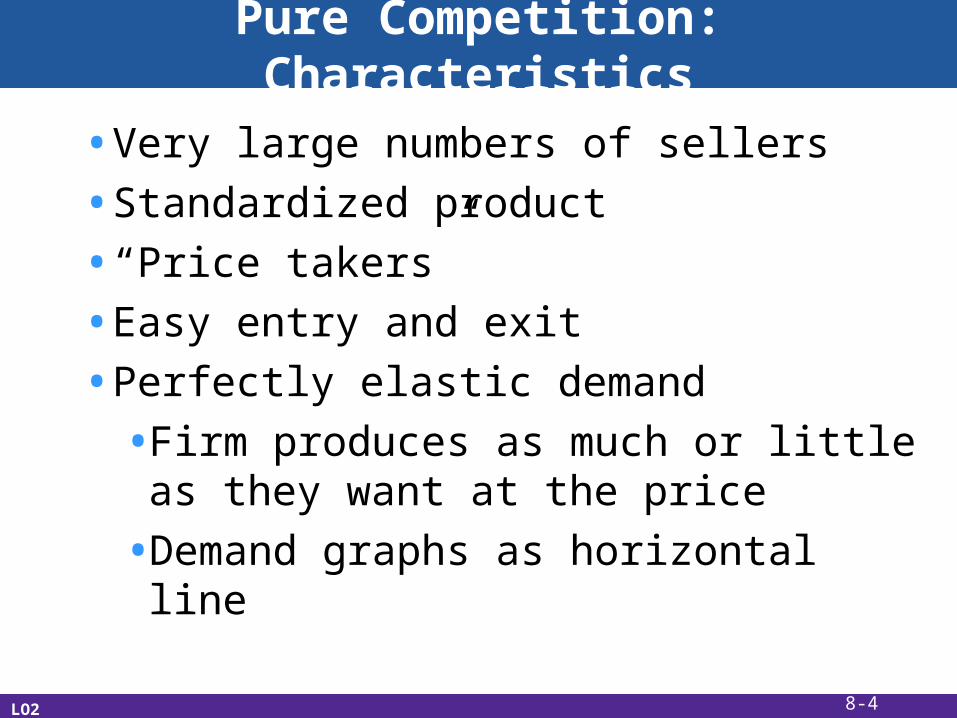
Pure Competition: Characteristics
• Very large numbers of sellers
• Standardized product
• “Price takers”
• Easy entry and exit
• Perfectly elastic demand
• Firm produces as much or little as they want at the price
• Demand graphs as horizontal line
LO2 8-4

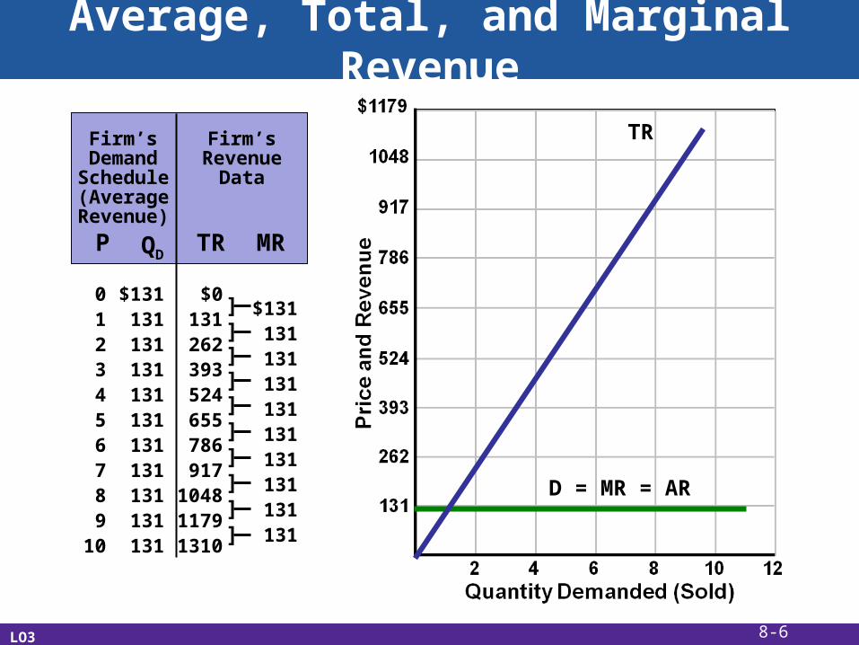
Average, Total, and Marginal Revenue
• Average Revenue
• Revenue per unit
• AR = TR/Q = P
• Total Revenue
• TR = P X Q
• Marginal Revenue
• Extra revenue from 1 more unit
• MR = ΔTR/ΔQ
LO3 8-5
Average, Total, and Marginal Revenue
LO3
Firm’sDemandSchedule(AverageRevenue)
Firm’sRevenue
Data
D = MR = AR
TR
P QDTR MR
$131131131131131131131131131131131
0123456789
10
$0131262393524655786917
104811791310
$131131131131131131131131131131
]]]]]]]]]]
8-6
Profit Maximization: TR-TC Approach
• Three questions:
• Should the firm produce?
• If so, what amount?
• What economic profit (loss) will be realized?
LO3 8-7

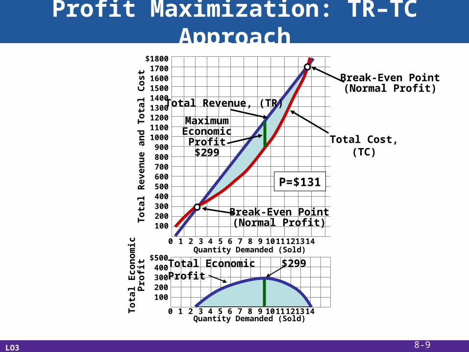
Profit Maximization: TR-TC Approach
LO3
The Profit-Maximizing Output for a Purely Competitive Firm: Total Revenue – Total Cost Approach (Price = $131)
(1)Total Product(Output) (Q)
(2)Total Fixed Cost (TFC)
(3)Total Variable Costs (TVC)
(4)Total Cost
(TC)
(5)Total
Revenue (TR)
(6)Profit (+)
or Loss (-)
0 $100 $0 $100 $0 $-100
1 100 90 190 131 -59
2 100 170 270 262 -8
3 100 240 340 393 +53
4 100 300 400 524 +124
5 100 370 470 655 +185
6 100 450 550 786 +236
7 100 540 640 917 +277
8 100 650 750 1048 +298
9 100 780 880 1179 +299
10 100 930 1030 1310 +280
8-8
10 2 3 4 5 6 7 8 9 10 11 1213 14
10 2 3 4 5 6 7 8 9 10 11 1213 14
$180017001600150014001300120011001000
900800700600500400300200100
$500400300200100
To
tal
Re
ven
ue
and
To
tal
Co
stT
ota
l E
con
om
icP
rofi
t
Quantity Demanded (Sold)
Quantity Demanded (Sold)
Profit Maximization: TR–TC Approach
LO3
Total Revenue, (TR)
Break-Even Point(Normal Profit)
Break-Even Point(Normal Profit)
MaximumEconomic
Profit$299
Total EconomicProfit
$299
P=$131
Total Cost,(TC)
8-9
Profit Maximization: MR-MC Approach
LO3
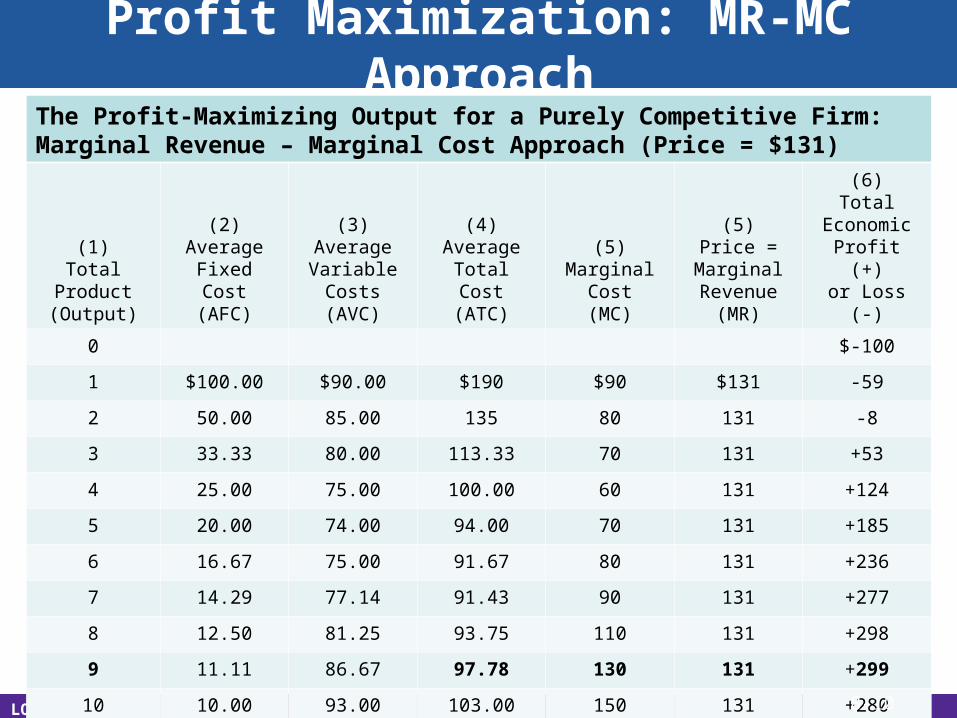
The Profit-Maximizing Output for a Purely Competitive Firm: Marginal Revenue – Marginal Cost Approach (Price = $131)
(1)Total
Product(Output)
(2)Average
Fixed Cost (AFC)
(3)Average Variable
Costs (AVC)
(4)Average
Total Cost(ATC)
(5)Marginal
Cost(MC)
(5)Price =
Marginal Revenue
(MR)
(6)Total
Economic Profit (+)
or Loss (-)
0 $-100
1 $100.00 $90.00 $190 $90 $131 -59
2 50.00 85.00 135 80 131 -8
3 33.33 80.00 113.33 70 131 +53
4 25.00 75.00 100.00 60 131 +124
5 20.00 74.00 94.00 70 131 +185
6 16.67 75.00 91.67 80 131 +236
7 14.29 77.14 91.43 90 131 +277
8 12.50 81.25 93.75 110 131 +298
9 11.11 86.67 97.78 130 131 +299
10 10.00 93.00 103.00 150 131 +280
8-10
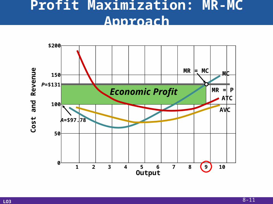
Profit Maximization: MR-MC Approach
LO3
Co
st a
nd
Rev
enu
e
$200
150
100
50
01 2 3 4 5 6 7 8 9 10
Output
Economic Profit MR = P
MCMR = MC
AVC
ATC
P=$131
A=$97.78
8-11
Loss-Minimizing Case
• Loss minimization
• Still produce because P > minAVC
• Losses at a minimum where MR=MC
LO3 8-12

Loss-Minimizing Case
LO3
Loss
MR = P
MC
AVCATC
P=$81
A=$91.67
V = $75
8-13
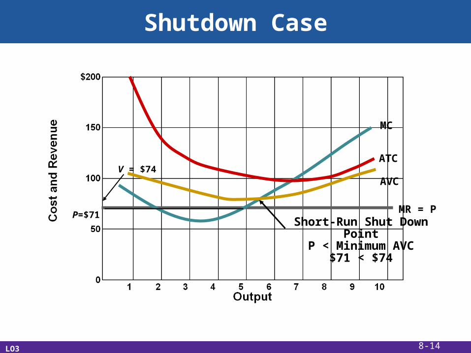
Shutdown Case
LO3
MR = P
MC
AVC
ATC
P=$71
V = $74
Short-Run Shut Down PointP < Minimum AVC
$71 < $74
8-14

Marginal Cost and Short-Run Supply
LO4
The Supply Schedule of a Competitive Firm Confronted with the Cost Data in the table in Figure 8.3
PriceQuantitySupplied
Maximum Profit (+)Minimum Loss (-)
$151 10 $+480
131 9 +299
111 8 +138
91 7 -3
81 6 -64
71 0 -100
61 0 -100
8-15

Marginal Cost and Short-Run Supply
LO4
P1
0
MR1
P2 MR2
P3 MR3
P4 MR4
P5 MR5
MC
AVC
ATC
Q2 Q3 Q4 Q5
ab
c
d
e
8-16

Marginal Cost and Short-Run Supply
LO4
P1
0
MR1
P2 MR2
P3 MR3
P4 MR4
P5 MR5
MC
AVC
ATC
Q2 Q3 Q4 Q5
ab
c
d
e
S
Shut-Down Point (If P is Below)
8-17
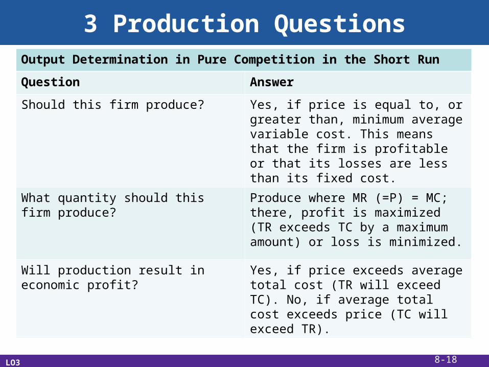
3 Production Questions
LO3
Output Determination in Pure Competition in the Short Run
Question Answer
Should this firm produce? Yes, if price is equal to, or greater than, minimum average variable cost. This means that the firm is profitable or that its losses are less than its fixed cost.
What quantity should this firm produce? Produce where MR (=P) = MC; there, profit is maximized (TR exceeds TC by a maximum amount) or loss is minimized.
Will production result in economic profit? Yes, if price exceeds average total cost (TR will exceed TC). No, if average total cost exceeds price (TC will exceed TR).
8-18
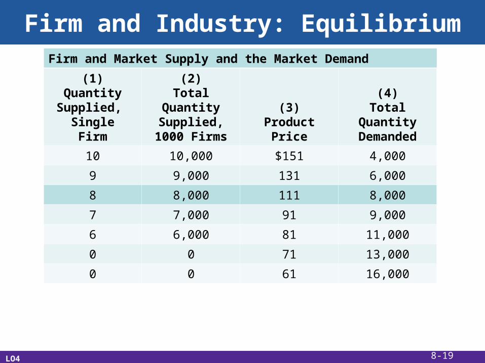
Firm and Industry: Equilibrium
LO4
Firm and Market Supply and the Market Demand
(1)Quantity
Supplied, SingleFirm
(2)Total
QuantitySupplied,
1000 Firms
(3)Product
Price
(4)Total
QuantityDemanded
10 10,000 $151 4,000
9 9,000 131 6,000
8 8,000 111 8,000
7 7,000 91 9,000
6 6,000 81 11,000
0 0 71 13,000
0 0 61 16,000
8-19
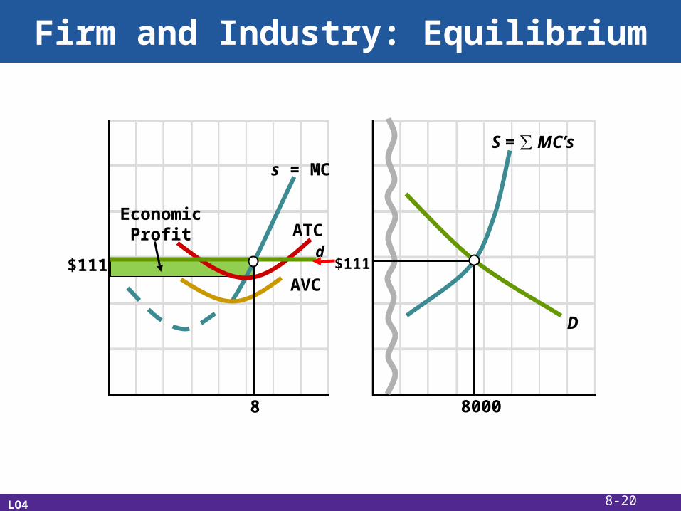
Firm and Industry: Equilibrium
LO4
EconomicProfit
dATC
AVC
s = MC
$111 $111
D
S = ∑ MC’s
8 8000
8-20
Fixed Costs: Digging Out of a Hole
• Shutting down in the short run does not mean shutting down forever
• Low prices can be temporary
• Some firms switch production on and off depending on the market price
• Examples: oil producers, resorts, and firms that shut down during a recession
8-21