purely dissipative solutions of navier-stokes equations

HAL Id: hal-02407364https://hal.archives-ouvertes.fr/hal-02407364

Preprint submitted on 12 Dec 2019

HAL is a multi-disciplinary open accessarchive for the deposit and dissemination of sci-entific research documents, whether they are pub-lished or not. The documents may come fromteaching and research institutions in France orabroad, or from public or private research centers.

L’archive ouverte pluridisciplinaire HAL, estdestinée au dépôt et à la diffusion de documentsscientifiques de niveau recherche, publiés ou non,émanant des établissements d’enseignement et derecherche français ou étrangers, des laboratoirespublics ou privés.

Purely dissipative solutions of Navier-Stokes equationsfor three-dimensional incompressible flows without wall

J Chai, T Wu, L Fang

To cite this version:J Chai, T Wu, L Fang. Purely dissipative solutions of Navier-Stokes equations for three-dimensionalincompressible flows without wall. 2019. �hal-02407364�

https://hal.archives-ouvertes.fr/hal-02407364

https://hal.archives-ouvertes.fr

This draft was prepared using the LaTeX style file belonging to the Journal of Fluid Mechanics 1

Purely dissipative solutions of Navier-Stokesequations for three-dimensional incompressible

flows without wall

J. Chai1, T. Wu1 and L. Fang1†1LMP, Ecole Centrale de Pekin, Beihang University, Beijing 100191, China

(Received xx; revised xx; accepted xx)

Existing analytical solutions of Navier-Stokes equations (NSE) are rare. Starting from the he-lical decomposition, we derive analytically a series of purely dissipative solutions of NSE forthree-dimensional incompressible flows without wall. The quasi-two-dimensional solutions aregeneralized Beltrami flows, and the three-dimensional solutions are find to be Beltrami flows.The two-dimensional Taylor-Green (TG) vortex and the Arnold-Beltrami-Childress (ABC) flowsare our particular solutions. By choosing N different wave vectors at the same wave length, oursolutions have 2N + 2 degrees of freedom for the quasi-two-dimensional cases and 2N degreesof freedom for the three-dimensional cases, indicating that the solution space can be at any highdimensions.

Key words:

1. IntroductionAlthough the properties of the solutions of Navier-Stokes Equations (NSE) still need a lot of

investigations, it is always interesting and important for us to search for the exact solutions ofNSE. Various exact solutions of NSE have been already introduced in previous studies (see Wang1991; Emanuel 2000), including a lot of famous laminar flows. In the following we will brieflyrevisit some of these exact solutions and emphasize the position of the present contribution. Forconsistency with the present contribution, we will restrict our discussion in three-dimensionalincompressible flows.

(i) Classic exact solutions of three-dimensional NSE usually considers special wall-boundedflows with self-similarity or under special boundary conditions. They can be approximatelyclassified into the following catalogs according to the type of boundary. a) Stationary parallelflows imply null velocity components perpendicular to the streamwise direction. Classic solu-tions include the Couette and Poieuille flows in straight channels, and the Hagen-Poiseuille flowin pipes. b) The rotating Couette flow is an extension of the plane Couette flow to cylindricalcoordinate. c) Non-stationary parallel flows consider the case that the velocity of boundary is notconstant, such as the accelerating boundary (i.e., the Rayleigh flow) and oscillating boundary. d)Other types of flows include the stagnation point flow, the Karman swirling flow, etc.. Since thepresent contribution will not discuss the wall-bounded flows, we will not visit more about therelated literature.

(ii) Another class of exact solutions of three-dimensional NSE considers the flows without

† Email address for correspondence: [email protected]

2 J. Chai, T. Wu and L. Fang

wall. These flows are usually either generalized Beltrami flows, i.e.,

∇ × (ω × u) = 0, (1.1)

where u is velocity and ω = ∇ × u is vorticity, or more strictly, Beltrami flows, i.e.,

ω × u = 0. (1.2)

Some exact solutions of these flows have been discussed in literature, for instance Hill (1894);Tsien (1943); Wang (1990a,b); Shi & Huang (1991); Shi et al. (1992); Fujimoto et al. (2015).Some of these solutions can be applied to wall-bounded cases, but the original solutions aresolved in infinite space without wall. Also, almost all these solutions are either axisymmetric orplanar flows. There are also several particular periodic solutions such as the two-dimensionalTaylor-Green (TG) vortex (Sipp & Jacquin 1998) and the Arnold-Beltrami-Childress (ABC)flows (Dombre et al. 1986).

In the present contribution, we will introduce a series of new solutions of NSE for three-dimensional flows without wall. These solutions are combined by any finite number of wavevectors in Fourier space, therefore they are periodic, rather than axisymmetric or planar. Wewill show that the quasi-two-dimensional solutions are generalized Beltrami flows, while thethree-dimensional solutions are Beltrami flows. The TG vortex and ABC flows are our particularsolutions. The solutions are therefore purely dissipative. Analysis of free degrees will show thatwe can obtain non-trivial solution space at any high dimension.

2. Helical decompositionIn the present contribution we consider the three-dimensional velocity field without wall, and

all velocity components are able to be represented in Fourier space. Following Constantin &Majda (1988); Waleffe (1992); Biferale et al. (2013), we can decompose an incompressiblevelocity field by using the helical decomposition. The velocity field v(x) in physical space istranslated to u(k) in Fourier space with k wave vector. Being divergence-free, k ·u(k) = 0, eachvelocity component in Fourier space has only two degrees of freedom. Two orthogonal complexhelical waves are chosen to be h± = w × k ± iw, with i =

√−1 and • unit vector. The vector w

can be chosen as w = (z × k)/∥z × k∥ with z an arbitrary vector. We then have

u(k) = u+z

(k)h+z

(k) + u−z

(k)h−z

(k), (2.1)

where u+z

and u−z

are complex numbers. The superscript z is emphasized here since thedecomposition depends on the selection of z. In Waleffe (1992) z is a constant vector, but inthe present contribution we will allow the change of z in order to obtain three-dimensionalsolutions. Constantin & Majda (1988) remarked that a single mode u+

z(k) or u−

z(k) corresponds

to a Beltrami field, then any incompressible velocity field can be considered as a superposition ofthese Beltrami unit flows. Researchers, such as Waleffe (1992); Biferale et al. (2012, 2013); Zhuet al. (2019), used this decomposition in the treatment of turbulence to investigate the forward andbackward energy backscatter. However, to our knowledge there is no discussion on combiningthese Beltrami unit flows to a complication NSE solution. In the present contribution we willdeal with this problem to obtain a class of new solutions.

Under the helical decomposition, the NSE can be rewritten as(∂t + νk2

)u(k) =

∑k+p+q=0

f (k, p, q)∑

sk ,sp,sq

skpq(skk + sp p + sqq)(sp p − sqq)uszp (p)uszq (q)hszk (k),

(2.2)where ν is viscosity, k = |k| is the wave length, z is always selected to be perpendicular top and q with the same direction as q × p (for example, the unit vector z = q × p) such that

Purely dissipative solutions of Navier-Stokes equations 3

f (k, p, q) = Q/(2kpq) is a geometrical factor with Q = (2k2 p2 + 2p2q2 + 2q2k2 − k4 − p4 − q4)1/2,skpq = sk spsq, • stands for complex conjugate, and sk, sp, sq = ± denote different helical modes.If the right hand side of Eq. (2.2) is zero for any wave vector k, we obtain purely dissipativesolutions

u(k, t) = u(k, t = 0)e−νk2t. (2.3)

If p and q are in the same direction, we will have f (k, p, q) = 0, leading to vanishing right-handside of Eq. (2.2). But for general cases it is complicated. In the present contribution we willtherefore aim at finding a set of wave vectorW, such that ∀p, q ∈ W,∑

sp,sq

skpq(skk + sp p + sqq)(sp p − sqq)uszp (p)uszq (q) ≡ 0 (2.4)

with k = −p − q and sk = ±. TransformingW and the conjugation part to physical space willdirectly lead to solution (2.3).

We remark that these flows are always generalized Beltrami flows. In fact, substituting (2.4)into (2.2) and taking the curl, we simply obtain

∂tω − ν∇2ω = 0. (2.5)

This is exactly the generalized Beltrami flow where ∇ × (ω × u) = 0 (see Wang 1991).

2.1. The case that p = q

Expanding Eq. (2.4) leads to

(p − q)(skk + p + q)u+z

(p)u+z

(q) − (p + q)(skk + p − q)u+z

(p)u−z

(q)

−(−p − q)(skk − p + q)u−z

(p)u+z

(q) + (−p + q)(skk − p − q)u−z

(p)u−z

(q) = 0.(2.6)

When p = q, this reduces to

(p + q)u+z

(p)u−z

(q) + (−p − q)u−z

(p)u+z

(q) = 0, (2.7)

or equivalentlyu+

z

(p)u−z

(q) − u−z

(p)u+z

(q) = 0, (2.8)This means that we can define a two-dimensional complex vector at a three-dimensional wavevector az(k) := (u+

z(k), u−

z(k)). When p = q, Eq. (2.4) is then equivalent to the parallel

condition between az(p) and az(q), denoted as

az(p) ∥ az(q). (2.9)

Note that this parallel condition is only defined when z is perpendicular to p and q. For anothervector ξ which is not perpendicular to both p and q, this condition will not be satisfied at thesame time. The proof is as follows.

As mentioned in Waleffe (1992), defining λ = (p) × q)/|p × q| (which is a unit vector parallelto z), we have

h±ξ

(p) = wξ(p) × p ± iwξ(p) = ei±φξp [λ ± iµ(p)] (2.10)where µ(p) = p × λ is located in the plane of the triad {k,p, q}, and φξp depends only on thedirection of ξ. Thus we obtain

h±ξ

(p) = ei±φξph±−λ

(p). (2.11)Particularly, after substituting ξ = λ into Eq. (2.11), we obtain φλp = π and φ−λp = 0. As u(p) isinvariant with the selection of the base of helical decomposition, u(p) can be rewritten under thenew base (hξ(p),h−ξ(p)) with

u+ξ

(p) = e−iφξpu+−λ

(p), u−ξ

(p) = eiφξpu−−λ

(p), (2.12)


and similarly for u(q). Then Eq. (2.8), which is satisfied when z = −λ, can be rewritten as

eiφξpu+ξ

(p)e−iφξqu−ξ

(q) − e−iφξpu−ξ

(p)eiφξqu+ξ

(q) = 0 (2.13)

Clearly, if ξ is not parallel to λ, the relation ei(φξp−φξq) = e−i(φξp−φξq) is not satisfied, thus Eq. (2.13)can not be transformed into the form (2.8), which means the parallel condition is not valid foraξ(p) and aξ(q) when ξ is not perpendicular to both p and q.

2.2. The case that p , q

When p , q, we separate the left-hand side of Eq. (2.6) in two parts P1(sk, p, q) and P2(k, p, q)

P1(sk, p, q) =(p2 − q2)sk

(u+

z

(p)u+z

(q) − u+z

(p)u−z

(q) − u−z

(p)u+z

(q) + u−z

(p)u−z

(q)),

P2(k, p, q) =(p − q)k(u+

z

(p)u+z

(q) − u−z

(p)u−z

(q))+ (p + q)(−k)

(u+

z

(p)u−z

(q) − u−z

(p)u+z

(q)).

(2.14)

Equation (2.6) should be satisfied for sk = ±1, which means

P1(1, p, q) + P2(k, p, q) =0,P1(−1, p, q) + P2(k, p, q) =0.

(2.15)

Due to the fact that P1(1, p, q) = −P1(−1, p, q), Eq. (2.15) leads to

P1(1, p, q) = P2(k, p, q) = 0, (2.16)

From Eqs. (2.14) and (2.16) we finally write

u+z

(p) = u−z

(p), u+z

(q) = u−z

(q). (2.17)

Since z is perpendicular to the plane of p, q and w(p) = (z×p)/|z×p| is chosen in the helicaldecomposition, we have w(p) × p = −z. From Eq. (2.17) we then obtain

u(p) =u+z

(p)(h+

z

(p) + h−z

(p))

=u+z

(p)(−2z)(2.18)

and similarly for u(q). Performing the inverse Fourier transform for this system with two vectorsas well as the conjugation leads to the velocity field

v(x) =u(p)eipx + u(q)eiqx + c.c.

=(u+

z

(p)eipx + u+z

(q)eiqx + c.c.)

(−2z),(2.19)

which indicates that all velocities must be in the z direction.In addition, performing the similar analysis as in the case that p = q, we will not have u+

ξ(p) =

u−ξ(p) and u+

ξ(p) = u−

ξ(p) if ξ is not perpendicular to both p and q.

Equation (2.19) indicates that when p , q, purely dissipative solutions are trivial quasi-one-dimensional flows, which will not involve interesting results. Therefore, in the presentcontribution we will only consider the flow whose wave vectors are of the same magnitude.

3. Quasi-two-dimensional flowsIn this section we will investigate the quasi-two-dimensional flows, which means that all

wave vectors in W are located in the same plane. In this case we can choose z a constantvector perpendicular to this plane, therefore in this section we will omit the superscript z in theequations. In this case we have the following lemma of transitivity.


Figure 1. Sketch of the system with four wave vectors uniformly distributed in (k1, k2) plane of spectralspace.

Lemma 1. If p, q and r are located in the same plane, a(p),a(q) and a(r) are non-nullcomplex vectors, and a(p) ∥ a(q),a(q) ∥ a(r), then a(p) ∥ a(r).

Proof. We select a cartesian coordinate (k1, k2, k3) such that p, q and r are located in the(k1, k2) plane, and z is in the k3 direction.

Supposing a(q) , 0, according to the parallel condition, a(p) ∥ a(q),a(q) ∥ a(r) leads to

a(p) = λ1a(q),a(q) = λ2a(r),

(3.1)

where (λ1, λ2) ∈ C2 and then we have

a(p) = λ1λ2a(r) (3.2)

which is equivalent to the parallel condition and we have directly a(p) ∥ a(r).

We can selectW ={p(1),p(2), ...,p(N)

}, where all wave vectors are located in the same plane

(k1, k2) with the same wave length. Let a(p(i)) ∥ a(p(i+1)) for i = 1, 2, ...,N−1. From Lemma 1 allthese wave vectors are then parallel to each other. Therefore, Eq. (2.4) is always satisfied, leadingto a purely dissipative solution (2.3). z is selected as z = (0, 0, 1) in the (k1, k2, k3) spectral space.

The above paragraphs describe a general method to generate purely dissipative quasi-two-dimensional velocity fields. In the following subsections, we will show several typical examples.

3.1. System with four wave vectors uniformly distributed

As shown in Fig.1, we start with a simple case by choosing W = {p, q} that has only twowave vectors with the same wavelength. Considering the conjugation set {−p,−q}, the wholesystem has four wave vectors. Specifially, these four wave vectors are assumed to be uniformlydistributed, i.e.,

p =

√

22 p√2

2 p0

, q =

√

22 p−√

22 p0

. (3.3)


Constraints of these wave vectors include the parallel conditions

a(p) ∥ a(q), a(q) ∥ a(−p), a(p) ∥ a(−p) (3.4)

and the conjugation conditions

a(p) = a(−p), a(q) = a(−q). (3.5)

These constraints lead to the general form of a(p) and a(q)

a(p) =(

Rpαp + IpαpiRpβp + Ipβpi

), a(q) =

(Rqαp + IqαpiRqβp + Iqβpi

), (3.6)

where (Rp, Ip,Rq, Iq, αp, βp) ∈ R6 are constants. Letting γp = αp + βp and σp = αp − βp, we have

u(p) =

√

22 Ipσp −

√2

2 Rpσpi−√

22 Ipσp +

√2

2 Rpσpi−Rpγp − Ipγpi

,u(q) =

−√

22 Iqσp +

√2

2 Rqσpi−√

22 Iqσp +

√2

2 Rqσpi−Rqγp − Iqγpi

, (3.7)

with (Rp, Ip,Rq, Iq, γp, σp) ∈ R6 constants, and the velocity field in physical space is then

v1(x1, x2, t = 0) =√

2Ipσp cos(

√2

2px1 +

√2

2px2) +

√2Rpσp sin(

√2

2px1 +

√2

2px2)

−√

2Iqσp cos(

√2

2px1 −

√2

2px2) −

√2Rqσp sin(

√2

2px1 −

√2

2px2)

v2(x1, x2, t = 0) = −√

2Ipσp cos(

√2

2px1 +

√2

2px2) −

√2Rpσp sin(

√2

2px1 +

√2

2px2)

−√

2Iqσp cos(

√2

2px1 −

√2

2px2) −

√2Rqσp sin(

√2

2px1 −

√2

2px2)

v3(x1, x2, t = 0) = − 2Rpγp cos(

√2

2px1 +

√2

2px2) + 2Ipγp sin(

√2

2px1 +

√2

2px2)

− 2Rqγp cos(

√2

2px1 −

√2

2px2) + 2Iqγp sin(

√2

2px1 −

√2

2px2)

(3.8)

Starting from this general expression, when p =√

2, γp = 0, Ip = 0, Iq = 0,Rp = Rq and2√

2σpRp = 1, we obtain the well-known solution of two dimensional TG vortex with v(x, t) =v(x, t = 0)e−2νt where v(x, t = 0) is

v1(x1, x2, t = 0) = cos(x1) sin(x2),v2(x1, x2, t = 0) = − sin(x1) cos(x2),v3(x1, x2, t = 0) =0.

(3.9)

3.2. System with six wave vectors uniformly distributed

The second example can be a system with six wave vectors of same wave length uniformlydistributed in the plane (k1, k2) of spectral space (see Fig. 2 as a sketch), that is,W = {p, q, r}with

p =

12 p√3

2 p0

, q =

12 p−√

32 p0

, r =

p00

(3.10)


Figure 2. Sketch of the system with six wave vectors uniformly distributed in (k1, k2) plane of spectralspace.

Similar to Sec. 3.1, for a(p),a(q) and a(r), the parallel conditions and conjugation conditionslead to

a(p) =(


), a(q) =


), a(r) =

(Rrαp + IrαpiRrβp + Irβpi

), (3.11)

where (Rp, Ip,Rq, Iq,Rr, Ir, αp, βp) ∈ R8 are constants. Letting γp = αp + βp and σp = αp − βp,we have

u(p) =

√

32 Ipσp −

√3

2 Rpσpi− 1

2 Ipσp +12 Rpσpi

−Rpγp − Ipγpi

,u(q) =

−√

32 Iqσp +

√3

2 Rqσpi− 1

2 Iqσp +12 Rqσpi

−Rqγp − Iqγpi

,u(r) =

0−Irσp + Rrσpi−Rrγp − Irγpi

,(3.12)

with (Rp, Ip,Rq, Iq,Rr, Ir, γp, σp) ∈ R8 constants, and the velocity field in physical space is then

v1(x1, x2) =√

3Ipσp cos(12

px1 +

√3

2px2) +

√3Rpσp sin(

12

px1 +

√3

2px2)

−√

3Iqσp cos(12

px1 −√

32

px2) −√

3Rqσp sin(12

px1 −√

32

px2)

v2(x1, x2) = − Ipσp cos(12

px1 +

√3

2px2) − Rpσp sin(

12

px1 +

√3

2px2) − 2Irσp cos(px1)

− Iqσp cos(12

px1 −√

32

px2) − Rqσp sin(12

px1 −√

32

px2) − 2Rrσp sin(px1)

v3(x1, x2) = − 2Rpγp cos(12

px1 +

√3

2px2) + 2Ipγp sin(

12

px1 +

√3

2px2) − 2Rrγp cos(px1)

− 2Rqγp cos(12

px1 −√

32

px2) + 2Iqγp sin(12

px1 −√

32

px2) + 2Irγp sin(px1)

(3.13)

For visualization, we artificially select the values of the constants and show the velocity com-ponents in Fig. 3. Note that this velocity field is independent to the third coordinate x3, but the


X

Y

Z

(a) v1(x1, x2)

X

Y

Z

(b) v2(x1, x2)

X

Y

Z

(c) v3(x1, x2)

Figure 3. Velocity components in physical space of the system with sixwave vectors uniformly distributed. As an example, constants are selected asp = 1,Rp = 3, Ip = 14,Rq = 6, Iq = 2,Rr = 12, Ir = 3, γp = 10, σp = −6 in Eq. (3.13). (a)v1(x1, x2), (b) v2(x1, x2), (c) v3(x1, x2).

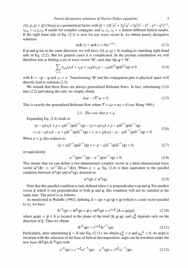
velocity vector has the third component v3, so it is not the same as the traditional two-dimensional(planar) flow. We name it as quasi-two-dimensional flow in the present contribution. This flowbelongs to a typical flow type (see Moffatt 1969) which was named as 3D2C by Zhu (2018).

As discussed in Sec. 2, we know that this solution is a generalized Beltrami flow. In order toshow that it is generally not Beltrami flow, we can calculate analytically the vorticity ω(x, t) =∇×v of the velocity field from Eq. (3.13). The isosurface of vorticity magnitude is shown in Fig.4, where periodical straight vortex tubes are observed. When γp , 0 and σp , 0, we find

ω1(x, t) = λ1v1(x, t),ω2(x, t) = λ2v2(x, t),ω3(x, t) = λ3v3(x, t),

(3.14)

where

λ1 = λ2 = pγp

σp, λ3 = p

σp

γp. (3.15)

Clearly, in the general case that γp , σp, we have λ1 = λ2 , λ3, which indicates that ω × v , 0and the flow is not a Beltrami flow.

3.3. System with six wave vectors non-uniformly distributed

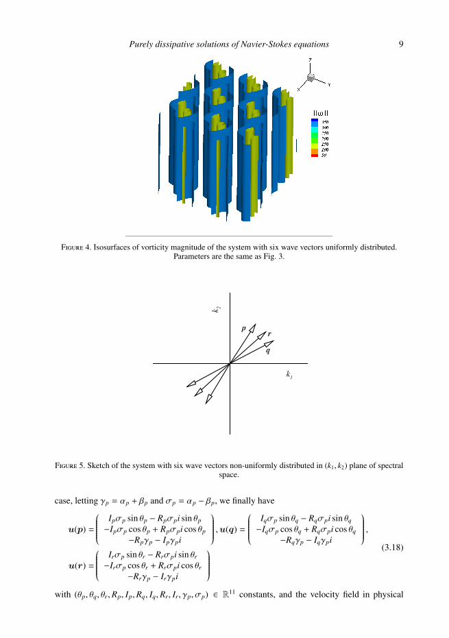
The parallel condition in (2.8) is only dependent to the helical-decomposed velocity com-poents, but is independent to the coordinates of wave vectors p and q. This means that the wavevectors can be artificially selected in the (k1, k2) plane in spectral space as long as there wavelengths are equal. In this subsection we then show the general cases of six-wave system. Aspresented in Fig. 5, we selectW = {p, q, r} with

p =

p cos θp

p sin θp

0

, q =

p cos θqp sin θq

0

, r =

p cos θrp sin θr

0

(3.16)

As the same as Sec. 3.2, we have

a(p) =(


), a(q) =


), a(r) =

(Rrαp + IrαpiRrβp + Irβpi

), (3.17)

where (Rp, Ip,Rq, Iq,Rr, Ir, αp, βp) ∈ R8 are constantsDifferences exist when substituting this to the helical decomposition. In the present general


Figure 4. Isosurfaces of vorticity magnitude of the system with six wave vectors uniformly distributed.Parameters are the same as Fig. 3.

Figure 5. Sketch of the system with six wave vectors non-uniformly distributed in (k1, k2) plane of spectralspace.

case, letting γp = αp + βp and σp = αp − βp, we finally have

u(p) =

Ipσp sin θp − Rpσpi sin θp

−Ipσp cos θp + Rpσpi cos θp

−Rpγp − Ipγpi

,u(q) =

Iqσp sin θq − Rqσpi sin θq−Iqσp cos θq + Rqσpi cos θq

−Rqγp − Iqγpi

,u(r) =

Irσp sin θr − Rrσpi sin θr−Irσp cos θr + Rrσpi cos θr

−Rrγp − Irγpi

(3.18)

with (θp, θq, θr,Rp, Ip,Rq, Iq,Rr, Ir, γp, σp) ∈ R11 constants, and the velocity field in physical


X

Y

Z

(a) v1(x1, x2)

X

Y

Z

(b) v2(x1, x2)

X

Y

Z

(c) v3(x1, x2)

Figure 6. Velocity components in physical space of the system with six wavevectors non-uniformly distributed. As an example, constants are selected asθp =

π3 , θq =

π6 , θr =

π4 , p = 1,Rp = 3, Ip = 14,Rq = 6, Iq = 2,Rr = 12, Ir = 3, γp = 10, σp = −6

in Eq. (3.19). (a) v1(x1, x2), (b) v2(x1, x2), (c) v3(x1, x2).

space is then

v1(x1, x2) =2Ipσp sin(θp) cos(px1 cos θp + px2 sin θp) + 2Rpσp sin(θp) sin(px1 cos θp + px2 sin θp)+2Iqσp sin(θq) cos(px1 cos θq + px2 sin θq) + 2Rqσp sin(θq) sin(px1 cos θq + px2 sin θq)+2Irσp sin(θr) cos(px1 cos θr + px2 sin θr) + 2Rrσp sin(θr) sin(px1 cos θr + px2 sin θr)

v2(x1, x2) = − 2Ipσp cos(θp) cos(px1 cos θp + px2 sin θp) − 2Rpσp cos(θp) sin(px1 cos θp + px2 sin θp)−2Iqσp cos(θq) cos(px1 cos θq + px2 sin θq) − 2Rqσp cos(θq) sin(px1 cos θq + px2 sin θq)−2Irσp cos(θr) cos(px1 cos θr + px2 sin θr) − 2Rrσp cos(θr) sin(px1 cos θr + px2 sin θr)

v3(x1, x2) = − 2Rpγp cos(px1 cos θp + px2 sin θp) + 2Ipγp sin(px1 cos θp + px2 sin θp)−2Rqγp cos(px1 cos θq + px2 sin θq) + 2Iqγp sin(px1 cos θq + px2 sin θq)−2Rrγp cos(px1 cos θr + px2 sin θr) + 2Irγp sin(px1 cos θr + px2 sin θr)

(3.19)

For visualization, we artificially select the values of the constants and show the velocity compo-nents in Fig. 6.

3.4. General form of quasi-two-dimensional flows with a finite number of wave vectors of thesame wavelength

From the three examples above, we observe that if one more wave vector is added toW of thesystem, two more independent variables will appear. In this subsection we then derive the generalform for any finite number of wave vectors. Considering a system with 2N wave vectors in the(k1, k2) plane includingW =

{p(1),p(2), ...,p(N)

}and their conjugations, supposing (α, β) ∈ R2,

with z = (0, 0, 1), we have the general form of a(p(i)), i = 1, 2, ...,N

a(p(i)) =(

Rp(i)α + Ip(i)αiRp(i)β + Ip(i)βi

), (3.20)

where (Rp(i) , Ip(i) ) ∈ R2 are two independent variables for each p(i). Letting γ = α+β andσ = α−β,we have the general form of u(p(i)), i = 1, 2, ...,N

u(p(i)) =

Ip(i)σ sin θp(i) − Rp(i)σi sin θp(i)

−Ip(i)σ cos θp(i) + Rp(i)σi cos θp(i)

−Rp(i)γ − Ip(i)γi

(3.21)


Inverse Fourier transform then leads to the general form of the velocity field in physical space

v(x) =N∑

i=1

u(p(i))eip(i)x

v1(x) =N∑

i=1

2Ip(i)σ sin(θp(i) ) cos(px1 cos θp(i) + px2 sin θp(i) )

+

N∑i=1

2Rp(i)σ sin(θp(i) ) sin(px1 cos θp(i) + px2 sin θp(i) )

v2(x) =N∑

i=1

(−2Ip(i) )σ cos(θp(i) ) cos(px1 cos θp(i) + px2 sin θp(i) )

+

N∑i=1

(−2Rp(i) )σ cos(θp(i) ) sin(px1 cos θp(i) + px2 sin θp(i) )

v3(x) =N∑

i=1

(−2Rp(i) )γ cos(px1 cos θp(i) + px2 sin θp(i) )

+

N∑i=1

2Ip(i)γ sin(px1 cos θp(i) + px2 sin θp(i) )

(3.22)

Where p is the wavelength for all wave vectors. There are in total 2N + 2 independent variablesin this expression of velocity field. As a result, for this quasi-two-dimensional system with 2Nwave vectors of the same wavelength, we have in total 2N + 2 degrees of freedom.

4. Three-dimensional flowsIn the last section all wave vectors are located in the same plane, leading to a quasi-two-

dimensional flow field which is independent to the x3 direction. In the previous section, we willdiscuss the case of three-dimensional flows. As discussed in Sec. 2.1, for a system whose wavevectors have the same wave length, the condition of being a purely dissipative system is that foreach two wave vectors p(i),p( j), choosing z perpendicular to them, az(pi) and az(p j) shouldsatisfy the parallel condition. Differing from the quasi-two-dimensional flows, here the vectorz can be different when considering different pair (p(i),p( j)), and the transitivity Lemma 1 isnot satisfied. This means that the parallelization of each pair (p(i),p( j)) can be considered asan independent constraint. In the following subsections we then show that we can also obtainthree-dimensional solutions, though the constraints are more complicated then the quasi-two-dimensional cases.

4.1. System with six wave vectors

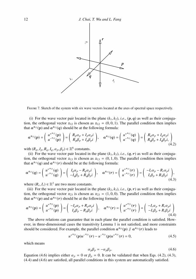
We start from a simple example where we have six wave vectors located at the three axes inspectral space respectively. In this case we haveW = {p, q, r} with

p =

0p0

, q =

p00

, r =

00p

. (4.1)

Figure 7 is a sketch for the wave vectors in spectral space. Visiting all wave vector pairs inthis set, we find that the pair is in a plane of either (k1, k2) or (k1, k3) or (k2, k3). The followingparagraphs will then involve the parallel conditions of them respectively.


Figure 7. Sketch of the system with six wave vectors located at the axes of spectral space respectively.

(i) For the wave vector pair located in the plane (k1, k2), i.e., (p, q) as well as their conjuga-tion, the orthogonal vector z12 is chosen as z12 = (0, 0, 1). The parallel condition then impliesthat az12 (p) and az12 (q) should be at the following formula:

az12 (p) =(

u+z12 (p)

u−z12 (p)

)=

(Rpαp + IpαpiRpβp + Ipβpi

), az12 (q) =

(u+

z12 (q)u−

z12 (q)

)=

(Rqαp + IqαpiRqβp + Iqβpi,

)(4.2)

with (Rp, Ip,Rq, Iq, αp, βp) ∈ R6 constants.(ii) For the wave vector pair located in the plane (k1, k3), i.e., (q, r) as well as their conjuga-

tion, the orthogonal vector z13 is chosen as z13 = (0, 1, 0). The parallel condition then impliesthat az13 (q) and az13 (r) should be at the following formula:

az13 (q) =(

u+z13 (q)

u−z13 (q)

)=

(Iqαp − Rqαpi−Iqβp + Rqβpi

), az13 (r) =

(u+

z13 (r)u−

z13 (r)

)=

(−Irαp − RrαpiIrβp + Rrβpi

),

(4.3)where (Rr, Ir) ∈ R2 are two more constants.

(iii) For the wave vector pair located in the plane (k2, k3), i.e., (p, r) as well as their conjuga-tion, the orthogonal vector z23 is chosen as z23 = (1, 0, 0). The parallel condition then impliesthat az23 (p) and az23 (r) should be at the following formula:

az23 (p) =(

u+z23 (p)

u−z23 (p)

)=

(−Ipαp + RpαpiIpβp − Rpβpi

), az23 (r) =

(u+

z23 (r)u−

z23 (r)

)=

(−Irαp + Rrαpi−Irβp + Rrβpi

)(4.4)

The above relations can guarantee that in each plane the parallel condition is satisfied. How-ever, in three-dimensional cases the transitivity Lemma 1 is not satisfied, and more constraintsshould be considered. For example, the parallel condition az23 (p) ∥ az23 (r) leads to

u+z23 (p)u−

z23 (r) − u−z23 (p)u+

z23 (r) = 0, (4.5)

which meansαpβp = −αpβp. (4.6)

Equation (4.6) implies either αp = 0 or βp = 0. It can be validated that when Eqs. (4.2), (4.3),(4.4) and (4.6) are satisfied, all parallel conditions in this system are automatically satisfied.


XY

Z

(a) v1(x1, x2, x3)

XY

Z

(b) v2(x1, x2, x3)

XY

Z

(c) v3(x1, x2, x3)

Figure 8. Velocity components in physical space of the system with six wave vectors. As an example,constants are selected as p = 1,Rp = 6, Ip = 28,Rq = 12, Iq = 4,Rr = 24, Ir = 6 in Eq. (4.8). (a)v1(x1, x2, x3), (b) v2(x1, x2, x3), (c) v3(x1, x2, x3).

Choosing without loss of generality βp = 0 and performing the inverse operation of helicaldecomposition, we have

u(p) =

Ipαp − Rpαpi0

−Rpαp − Ipαpi

, u(q) =

0−Iqαp + Rqαpi−Rqαp − Iqαpi

, u(r) =

Rrαp − IrαpiIrαp + Rrαpi

0

, (4.7)

Note that αp appears in all terms which indicates that the choice of it has no influence on the formof u and we can eliminate it. The system has only 6 degrees of freedom. Then the correspondingvelocity field in physical space becomes

v(x1, x2, x3, t = 0) =

2Ip cos(px2) + 2Rp sin(px2) + 2Rr cos(px3) + 2Ir sin(px3)−2Iq cos(px1) − 2Rq sin(px1) + 2Ir cos(px3) − 2Rr sin(px3)−2Rp cos(px2) + 2Ip sin(px2) − 2Rq cos(px1) + 2Iq sin(px1)

. (4.8)

We can also write this solution with defining another set of symbols

A = 2Ir, B = −2Rq, C = 2Ip,

A′ = −2Rr, B′ = 2Iq, C′ = 2Rp,(4.9)

and obtain

v(x1, x2, x3, t = 0) =

A sin(px3) +C cos(px2)B sin(px1) + A cos(px3)C sin(px2) + B cos(px1)

+ −A′ cos(px3) +C′ sin(px2)−B′ cos(px1) + A′ sin(px3)−C′ cos(px2) + B′ sin(px1)

(4.10)

The first part in the right-hand side is the ABC flows, while the second part is a symmetric form.When A′ = B′ = C′ = 0 this system is simplified to the ABC flows.

It is possible to validate analytically that the vorticity of this flow field is always parallel to thevelocity field, i.e.,

ω(x, t) = λv(x, t) (4.11)with λ constant. This means that the present solutions are Beltrami flows.

For visualization, we artificially select the values of the constants and show the velocitycomponents in Fig. 8. The isosurfaces of vorticity magnitude is also shown in Fig.9.

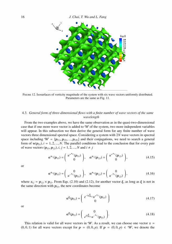
4.2. System with eight wave vectors

In this subsection, we consider a more complicated problem with eight wave vectors. Six ofthem are located in the (k1, k2) plane, while the other two are at the k3 axis (see Fig. 10 as a



Figure 10. 8 wave vectors of same wavelength, 2 wave vectors overlap with k3 axis in spectral space andthe other 6 wave vectors uniformly distributed in k1, k2 plane

sketch). Specifically, the setW = {p, q, r, s} is

p =

12 p√3

2 p0

, q =

12 p−√

32 p0

, r =

p00

, s =

00p

(4.12)

In this case, we have four different planes for different pairs of wave vectors. Using the same


XY

Z

(a) v1(x1, x2, x3)

XY

Z

(b) v2(x1, x2, x3)

XY

Z

(c) v3(x1, x2, x3)

Figure 11. The cloud maps for components of velocity vector at t = 0 for the flow field in physical space.Asan example, constants are select as p = 1,Rp = 6, Ip = 28,Rq = 12, Iq = 4,Rr = 24, Ir = 6,Rs = 2, Is = 38in Eq. (4.14). (a) v1(x1, x2, x3), (b) v2(x1, x2, x3), (c) v3(x1, x2, x3)

method as Sec. 4.1, finally we have

u(p) =

√

32 Ip −

√3

2 Rpi− 1

2 Ip +12 Rpi

−Rp − Ipi

,u(q) =

−√

32 Iq +

√3

2 Rqi− 1

2 Iq +12 Rqi

−Rq − Iqi

,u(r) =

0−Ir + Rri−Rr − Iri

,u(r) =

Rs − IsiIs + Rsi

0

,(4.13)

where (Rp, Ip,Rq, Iq,Rr, Ir,Rs, Is) ∈ R8 are constants. The velocity components in physical spaceare

v1(x1, x2, x3, t = 0) =√

3Ip cos(12

px1 +

√3

2px2) +

√3Rp sin(

12

px1 +

√3

2px2)

−√

3Iq cos(12

px1 −√

32

px2) −√

3Rq sin(12

px1 −√

32

px2)

+2Rs cos(px3) + 2Is sin(px3)

v2(x1, x2, x3, t = 0) = − Ip cos(12

px1 +

√3

2px2) − Rp sin(

12

px1 +

√3

2px2)

−Iq cos(12

px1 −√

32

px2) − Rq sin(12

px1 −√

32

px2)

−2Ir cos(px1) − 2Rr sin(px1) + 2Is cos(px3) − 2Rs sin(px3)

v3(x1, x2, x3, t = 0) = − 2Rp cos(12

px1 +

√3

2px2) + 2Ip sin(

12

px1 +

√3

2px2)

−2Rq cos(12

px1 −√

32

px2) + 2Iq sin(12

px1 −√

32

px2)

−2Rr cos(px1) + 2Ir sin(px1)

(4.14)

For visualization, we artificially select the values of the constants and show the velocitycomponents in Fig. 11. The isosurfaces of vorticity magnitude is also shown in Fig.12.

For this system, the analysis of vorticity vector gives the same property that indicates this flowalso a Beltrami flow.



4.3. General form of three-dimensional flows with a finite number of wave vectors of the samewavelength

From the two examples above, we have the same observation as in the quasi-two-dimensionalcase that if one more wave vector is added toW of the system, two more independent variableswill appear. In this subsection we then derive the general form for any finite number of wavevectors three dimensional spectral space. Considering a system with 2N wave vectors in spectralspace including W =

{p(1),p(2), ...,p(N)

}and their conjugations, we need to search a general

form of u(p(i)), i = 1, 2, ...,N. The parallel conditions lead to the conclusion that for every pairof wave vectors (p(i),p( j)), i, j = 1, 2, ...,N and i , j

azi j (p(i)) =(

u+zi j (p(i))

0

), azi j (p( j)) =

(u+

zi j (p( j))0

), (4.15)

or

azi j (p(i)) =(

0u−

zi j (p(i))

), azi j (p( j)) =

(0

u−zi j (p( j))

), (4.16)

where zi j = p( j) × p(i). From Eqs. (2.10) and (2.12), for another vector ξ, as long as ξ is not inthe same direction with p(i), the new coordinates become

aξ(p(i)) = e−iφξp(i) u+

zi j (p(i))0

(4.17)

or

aξ(p(i)) = 0

eiφξp(i) u−zi j (p(i))

. (4.18)

This relation is valid for all wave vectors in W. As a result, we can choose one vector z =(0, 0, 1) for all wave vectors except for p = (0, 0, p). If p = (0, 0, p) ∈ W, we denote the


coordinates of other wave vectors as

p(i) =

k1p(i)

pk2p(i)

pk3p(i)

p

,∀i = 1, 2, ...,N − 1, (4.19)

where p is the wavelength, k21p(i)+ k2

2p(i)+ k2

3p(i)= 1 and k2

1p(i)+ k2

2p(i), 0. For i = N, we write

p(N) =

00p

. (4.20)

With these notations, we can have the general form of az(p(i)), i = 1, 2, ...,N − 1

az(p(i)) =(

Rp(i) + Ip(i) i0

)(4.21)

or

az(p(i)) =(

0Rp(i) + Ip(i) i

), (4.22)

where (Rp(i) , Ip(i) ) ∈ R2 are two independent variables for each wave vector. For the case in whichwe use the general form of az(p(i)), i = 1, 2, ...,N−1 in Eq. (4.21), we have u(p(i)), i = 1, 2, ...,N−1

h+z

(p(i)) =

k1p(i)

k2p(i)− k2p(i)

ik2p(i)

k3p(i)+ k1p(i)

i−k2

1p(i)− k2

2p(i)

,u(p(i)) =

(Rp(i) k1p(i)

k2p(i)+ Ip(i) k2p(i)

) + (Ip(i) k1p(i)k2p(i)− Rp(i) k2p(i)

)i(Rp(i) k2p(i)

k3p(i)− Ip(i) k1p(i)

) + (Ip(i) k2p(i)k3p(i)+ Rp(i) k1p(i)

)i−Rp(i) (k

21p(i)+ k2

2p(i)) − Ip(i) (k

21p(i)+ k2

2p(i))i

.(4.23)

For i = N, we have

u(p(N)) =

Rp(N) − Ip(N) iIp(N) + Rp(N) i

0

(4.24)

Inverse Fourier transform then leads to the general form of velocity field in physical space for


this case

v1(x, t = 0) =N−1∑i=1

2(Rp(i) k1p(i)k2p(i)+ Ip(i) k2p(i)

) cos(k1p(i)x1 + k2p(i)

x2 + k3p(i)x3) + 2Rp(N) cos(px3)

+

N−1∑i=1

(−2)(Ip(i) k1p(i)k2p(i)− Rp(i) k2p(i)

) sin(k1p(i)x1 + k2p(i)

x2 + k3p(i)x3) + 2Ip(N) sin(px3),

v2(x, t = 0) =N−1∑i=1

2(Rp(i) k2p(i)k3p(i)− Ip(i) k1p(i)

) cos(k1p(i)x1 + k2p(i)

x2 + k3p(i)x3) + 2Ip(N) cos(px3)

+

N−1∑i=1

(−2)(Ip(i) k2p(i)k3p(i)+ Rp(i) k1p(i)

) sin(k1p(i)x1 + k2p(i)

x2 + k3p(i)x3) − 2Rp(N) sin(px3),

v3(x, t = 0) =N−1∑i=1

(−2)Rp(i) (k21p(i)+ k2

2p(i)) cos(k1p(i)

x1 + k2p(i)x2 + k3p(i)

x3)

+

N−1∑i=1

2Ip(i) (k21p(i)+ k2

2p(i)) sin(k1p(i)

x1 + k2p(i)x2 + k3p(i)

x3).

(4.25)

If p = (0, 0, p) <W, we just eliminate the components associated with cos(px3) and sin(px3).We can also use the spherical coordinates to represent k1p(i)

, k2p(i)and k3p(i)

and introduce theangles in Eq. (4.25) similar as the method in Sec. 3.4. We have k1p(i)

= sin θp(i) cos ϕp(i) , k2p(i)=

sin θp(i) sin ϕp(i) , k3p(i)= cos θp(i) .

For the other case in which the general form of az(p(i)), i = 1, 2, ...,N − 1 is Eq. (4.22), wecan perform a similar derivation and obtain another general form of velocity similar to the onepresented.

From these general results for three-dimensional flows, we can conclude on the degrees offreedom that for a three dimensional system with N wave vectors of the same wavelength, wehave 2N degrees of freedom.

5. Concluding remarksStarting from the helical decomposition, we derive analytically a series of purely dissipative

solutions of NSE for three-dimensional incompressible flows without wall. The quasi-two-dimensional solutions are generalized Beltrami flows, and the three-dimensional solutions are,according to present examples, Beltrami flows. The two-dimensional TG vortex and the ABCflows are our particular solutions. Although not rigorously proved, we guess that these solutionsmight be general non-trivial solutions for the cases that flow is three-dimensional, incompress-ible, and can be presented via a summation of a finite number of discrete Fourier wave modes.This is suggested as an open question.

The present solutions are complementations to existing analytical solutions of NSE. In fact,our solutions can be expanded to any high degree of freedom, indicating that the solution spacecan be at any high dimensions. For the stabilities of these solutions, we have numerically testedsome examples and found they are all instable. Rigorous proves are required in the future studies.

This result might also involve new understandings about the generation and energy transferof turbulence. Imaging two different flow fields: the first flow is one of our solutions, while thesecond flow changes the phases at one or more wave vectors, such at the parallel condition (2.8)is not always satisfied. Clearly, these two flows have exactly the same energy distribution, buttheir behaviors of energy transfer are different: the first flow does not have any multi-scale energy


exchange, but the second flow will exchange energy to smaller scales. In fact, we illustrated inSecs. 2.1 and 2.2 that if a system contains different wave lengths, energy will (non-trivially)transfer, but for a system with only one wave length, energy transfer does not always happen. Toquantitatively measure the multi-scale energy transfer, a quantity based on the parallel condition(2.8) might be appropriate. For example, we could define the complex angle between az(p) andaz(q) at a fixed wave length to estimate whether this scale is likely to transfer energy to otherscales. We expect that these ideas might inspire future studies.

AcknowledgementWe are grateful to Xinting Zhang, Haitao Xu, Ying Zhu, Claude Cambon and Wouter Bos

for inspiring discussions. This work is supported by the National Natural Science Foundation ofChina (Grant No.s 11572025, 11772032, 51420105008).

REFERENCES

Biferale, L., Musacchio, S. & Toschi, F. 2012 Inverse energy cascade in three-dimensional isotropicturbulence. Phys. Rev. Lett. 108, 164501.

Biferale, L., Musacchio, S. & Toschi, F. 2013 Split energy-helicity cascades in three-dimensionalhomogeneous and isotropic turbulence. J. Fluid Mech. 730, 309–327.

Constantin, P. & Majda, A. 1988 The Beltrami spectrum for incompressible fluid flows. Commun. Math.Phys. 115, 435–456.

Dombre, T., Frisch, U., Greene, J. M., Henon, M. & Soward, A. M. 1986 Chaotic streamlines in the abcflows. Journal of Fluid Mechanics 167, 353–391.

Emanuel, G. 2000 Analytical Fluid dynamics. CRC Press.Fujimoto, Minoru, Uehara, Kunihiko & Yanase, Shinichiro 2015 Vortex solutions of the generalized

Beltrami flows to the incompressible Euler equations. arXiv preprint arXiv:1501.05620 .Hill, M.J.M. 1894 On a spherical vortex. Philos. Trans. R. Soc. London Ser. A 185, 213–45.Moffatt, H.K. 1969 The degree of knottedness of tangled vortex lines. Journal of Fluid Mechanics 35,

117–129.Shi, C.C. & Huang, Y.N. 1991 Some properties of three-dimensional Beltrami flows. Acta Mechanica Sinica

7 (4), 289–294.Shi, C.C., Huang, Y.N. & Chen, Y.S. 1992 On the Beltrami flows. Acta Mechanica Sinica 8 (4), 289–294.Sipp, D. & Jacquin, L. 1998 Elliptic instability in two-dimensional flattened taylorgreen vortices. Physics of

Fluids 10 (4), 839.Tsien, H.S. 1943 Symmetrical Joukowsky airfoils in shear flow. Q. Appl. Math. 1, 130–48.Waleffe, F. 1992 The nature of triad interactions in homogeneous turbulence. Physics of Fluids A 4 (2),

350–363.Wang, C.Y. 1990a Exact solution of the Navier-Stokes equations — the generalized Beltrami flows, review

and extension. Acta Mech. 81, 69–74.Wang, C.Y. 1990b Shear flow over convection cells — an exact solution of the Navier-Stokes equations.

ZAMM Journal of Applied Mathematics and Mechanics 70 (8), 351–352.Wang, C.Y. 1991 Exact solutions of the steady-state Navier-Stokes equations. Annu. Rev. Fluid Mech. 23,

159–77.Zhu, J.Z. 2018 Vorticity and helicity decompositions and dynamics with real Schur form of the velocity

gradient. Physical of Fluids 30, 031703.Zhu, Y., Cambon, C., Godeferd, F.S. & Salhi, A. 2019 Nonlinear spectral model for rotating sheared

turbulence. Journal of Fluid Mechanics 866, 5–32.

purely dissipative solutions of navier-stokes equations

Documents