purse seine fishery management in malaysia : an output
TRANSCRIPT

Instructions for use
Title Purse seine fishery management in Malaysia : an output control for sustainable fisheries
Author(s) Harlyan, Ledhyane Ika
Citation 北海道大学. 博士(水産科学) 甲第13736号
Issue Date 2019-09-25
DOI 10.14943/doctoral.k13736
Doc URL http://hdl.handle.net/2115/80364
Type theses (doctoral)
File Information Ledhyane_Ika_Harlyan.pdf
Hokkaido University Collection of Scholarly and Academic Papers : HUSCAP

i
Purse seine fishery management in Malaysia
: an output control for sustainable fisheries
(マレーシアにおけるまき網漁業管理: 持続可能な漁業のための産出量規制)
北海道大学大学院水産科学院
海洋生物資源科学専攻
Graduate School of Fisheries Sciences
Division of Marine Bioresource and Environmental Science
レディヤヌ イカ ハルリヤン
Ledhyane Ika Harlyan
2019年

i
ABSTRACT
I. Introduction
Southeast Asia (SEA) region is a promising region to provide a continuously increasing capture
fishery production. Among SEA countries, Malaysia is the best practice model and a leading country
for estimating best management strategies that promote sustainable fisheries practices. Purse seine
fishery have played an important role in Malaysian fisheries for small, pelagic, economically important
fishes, not only for food consumption, but also for supporting the livelihoods and employment of
fishers. Over the past 10 years, purse seine fishing capacity has increased with minor changes in
species composition for all species. However, it is still important to examine the sustainability of the
Malaysian purse seine fishery as the fishing capacity has progressively increased.
To maintain sustainability, three management measures can be considered: input control,
technical control, and output control. The Malaysian Government has conducted input and technical
controls, but output control has not been implemented yet, although a pilot project and feasibility study
began in the East Coast Peninsular Malaysia (ECPM) in 2015. Prior to starting a quota system, the
fishery managers set a total allowable catch (TAC) as an annual catch limit, which is usually based
on scientific advice or catch data known as allowable biological catch (ABC). It requires data of each
species individually fitted and applied in single-species stock management models. However, most
fisheries, including Malaysian fisheries, involve multiple stocks or multiple fleets competing for the
same fish resources. Therefore, to implement a quota system in the multispecies purse seine fishery
in Malaysia, information of species such as habitat and seasonal life stages is needed. It is critical to
confirm whether the purse seine fishery as a multi-species fishery in Malaysia can be easily localized
by areas (spatially) or by seasons (temporally) before the implementation of output control.
II. Overview of the purse seine fishery in Malaysia
To confirm the feasibility of output control, concerning on its limitations and requirements, towards
Malaysian purse seine fishery, an overview of purse seine fishery in Malaysia was given by clarifying
the spatial and temporal patterns of purse seine fishing areas and seasons through species diversity
and cluster analysis. The analyses showed no specific seasonal and temporal pattern in the structure
of the purse seine fishery fishing grounds in ECPM areas. Huge species aggregations in catch
categories lead to incapability of providing species-separated data.
Multispecies fisheries are subjected to widely distributed and homogenously mixed fish
stocks which lead to non-selective exploitation. Therefore, realizing the multispecies fishery condition
in Malaysian fisheries, it is impractical to manage each species individually using single-species stock
assessment in multispecies fisheries. A tactical short-term management approach can be an option
to respond to the demands of data-limited management, which might occur in a multispecies fishery.

ii
III. Proposed management measure for purse seine fishery in Malaysia: an output control for
sustainable fisheries
A short-term management approach that can deal with multispecies fisheries in ECPM is the
feedback harvest control rule (HCR), which has been successfully applied in Japanese fisheries
management, called the ABC rule 2-1 in the Japanese TAC system. This feedback HCR was
previously validated to be applied in fisheries with a single-species approach. By combining
management strategy evaluation with a simulation to generate mixed-species data from a
multispecies fishery, the performance of this feedback HCR was evaluated and then compared with
its performance using species-specific data. Also, the sensitivity of the feedback HCR’s performance
over several scenarios of population dynamics was also examined and compared across other
modified HCRs.
The results showed that the feedback HCR is appropriate for multispecies fisheries management
where only mixed-species data are available but with special monitoring for slow-growing minor
species. In other words, the feedback HCR presents an initial step toward sustainably managing
multispecies fisheries while contending with data-limited conditions.
IV. Concluding discussion
The Malaysian purse seine fishery management needs to commit to maintaining sustainable
fisheries. It can be done by considering establishing input control through a clear and accurate
adjustment of fishing capacity; strengthen capacity and capability for regional cooperation, in
particular regional coordination meetings and joint surveillance with neighboring countries; and the
implementation of output control.
A combination of input and output controls will be the best option for providing sustainable fisheries
management for Malaysian fisheries and other multispecies fisheries in the region. The limitation of
output control implementation towards multispecies fisheries condition can be solved by conducting
the feedback HCR which was validated dealing with data-limited conditions. As a merit, the feedback
HCR is designed to attain an optimum catch and biomass along with less catch variation which will
simultaneously affect fisheries sustainability.
This research pointedly suggests that data-limited multispecies fisheries can be managed
sustainably using multiple management measures, such as a combination of input, output and
technical controls. Furthermore, the availability of reliable species-specific data for certain major
species and mixed-species data for other species will generate substantial progress for fisheries
management in SEA.

iii
TABLE OF CONTENTS
ABSTRACT ........................................................................................................................ i
TABLE OF CONTENTS .................................................................................................... iii
ACKNOWLEDGEMENTS .................................................................................................. iv
1. INTRODUCTION ........................................................................................................... 1
1.1. Characteristics of Southeast Asian (SEA) fisheries .................................................. 1
1.2. Exemplary fisheries management in Malaysia .......................................................... 4
1.3. General measures of fisheries management ............................................................ 7
1.4. Purse seine fishery management in Malaysia ........................................................... 9
1.5 Aim of this study ..................................................................................................... 14
1.6 Structure of the thesis ............................................................................................ 15
2. OVERVIEW OF THE PURSE SEINE FISHERY IN MALAYSIA .................................. 16
2.1. Background ............................................................................................................ 16
2.2. Materials and Methods ........................................................................................... 18
2.3. Results ................................................................................................................... 24
2.4. Discussion .............................................................................................................. 27
3. PROPOSED MANAGEMENT MEASURES FOR THE PURSE SEINE FISHERY IN
MALAYSIA: AN OUTPUT CONTROL FOR SUSTAINABLE FISHERIES ................... 33
3.1. Background ............................................................................................................ 33
3.2. Materials and Methods ........................................................................................... 35
3.3. Results .................................................................................................................. 41
3.4. Discussion ............................................................................................................. 44
4. GENERAL CONCLUSIONS ....................................................................................... 50
REFERENCES ................................................................................................................ 55
TABLES .......................................................................................................................... 65
FIGURES ......................................................................................................................... 73
APPENDICES................................................................................................................ 100

iv
ACKNOWLEDGEMENTS
First and foremost, I would like to thank Allah for giving me strength and opportunity to
undertake this doctoral study and to persevere and complete it satisfactorily. الحمد لله ربّ العالمين
Without his blessings, I would not have been possible.
In my journey towards this degree, I have found a teacher and a pillar of support, Prof.
MATSUISHI Takashi. I would like to express my sincere gratitude for his continuous support,
his patience, motivation and immense knowledge. His guidance helped me in all the time of
research and writing of this thesis. All his advices assisted me to have great living experience
in Japan.
I also would like to thank the rest of my thesis committee: Prof. TAKATSU Tetsuya, Prof.
FUJIMORI Yasuzumi and Prof. John Bower, for their valuable insightful suggestions that
incented me to improve my thesis from various perspectives. In addition, for the entire staff
at Faculty of Fisheries Sciences, Hokkaido University, who have always been so helpful
and cooperative in giving their support for academic affairs.
A very special gratitude goes out to the Indonesia Endowment Fund for Education (LPDP)
and the Southeast Asian Fisheries Development Center (SEAFDEC) for providing the
funding for the work. Also, to Department of Fisheries Malaysia, Jabatan Perikanan
Malaysia, for giving me great opportunity exploring the Malaysian purse seine fishery and
providing me various invaluable supporting documents.
To all my fellows in Matsuishi-Ken, MATSUDA Ayaka, KURODA Mika, Khuu Thi Phuong
Dong, MATSUI Natsuki, MAEDA Saki, YOSHIYAMA Taku, WU Dengke, KINASHI
Ryosuke, MUNEHARA Masami, Suppapong Pattarapongpan, TAKANO Keiko, KANNO
Hayato, TAGE Kaori, YAMAMOTO Aito and Pran Chavalittumrong, I thank you for all
great times we have had in the last three years.
I take pride in acknowledging my institution, Faculty of Fisheries and Marine Science
Brawijaya University, to give me an opportunity to pursue my study. Also, for MEXMA-UB
for encouraging and giving me chance to still contribute in remarkable activities during my
study.
My acknowledgement would be incomplete without thanking the biggest source of my
strength, my family. To my loves of my life, Herbhirawa & Dastan, for their love and care
that always brighten my days now and forever. Also, to my parents Bapak Harsono & Ibu
Ellyana, Bapak Sumaryono & Ibu Laila Tsalasih, Tante Diyang, brothers & sisters
Gendhy Dwi Harlyan & Festi Winda Sari, Dewi Handzani & Azharul ulum Syabana,
Gusti Arya Seta & Ratih Fitriyani, and my relatives for all their prayers at all times.
Ledhyane Ika Harlyan

1
1. INTRODUCTION
1.1. Characteristics of Southeast Asian (SEA) fisheries
The United Nations’ 2030 Agenda for Sustainable Development (2030 Agenda) and its
Sustainable Development Goals (SDGs) provide an integrative approach to improve the
world to a sustainable and resilient path that leaves none behind, particularly supporting
developing countries to achieve their economic interdependencies. Related to fisheries,
SDG 14 fully concerns conservation and sustainable use of the oceans, seas and marine
resources for sustainable development. SDG 14 and its targets have continued their efforts
to regulate harvesting by implementing science-based management plans and ending all
destructive fishing practices such as overfishing, illegal, unreported and unregulated (IUU)
fishing to restore fish stocks to the levels that can produce the maximum sustainable yield
(MSY) as determined by their biological characteristics. Other SDGs that are also relevant
with fisheries are as follows: fisheries value chain for supporting the poor livelihoods (SDG
1), fish for combating zero hunger (SDG 2), fisheries for contributing to good health and well-
being (SDG 3), fisheries for establishing economic growth (SDG 8), reductions in fishery
post-harvest losses (SDG 12), and low environmental climate impact of fisheries and
aquaculture compared to other food sources (SDG 13). In the other words, for achieving the
2030 Agenda and its SDGs, the global community needs to promote sustainability in
fisheries as a food supply in developing countries as well as it is done in developed countries
(FAO 2018).
In 2016, the global fish production peaked at about 171 million tons, with static capture
fishery production since the late 1980s and progressive growth of aquaculture to compose
about 47% of total production. The stable trend of capture fishery has been mainly due to
the declining catches of some regions. According to The State of World Fisheries and
Aquaculture 1988 – 2018, in the world’s most productive capture fishery areas, the Northern
and the Southern Pacific Ocean, capture fishery production has declined, while in other
regions, it has remained steady. Only three regions, the Western Central Pacific, the Eastern

2
and the Western Indian Ocean, have had a continuously increasing trend in capture fishery
production to compensate for declines in the other regions and to stabilize the world capture
fishery productions by composing the highest proportion of biologically sustainable stocks
at 72.6% (FAO 2018).
Southeast Asia (SEA) countries have played an important role in the increased fishing
capacity in the world through enhancing the numbers of fishers and motorized fishing
vessels (SEAFDEC 2015a, 2017, FAO 2018). It is believed that increased fishing capacity
might cause increased fishery landings (Sumaila et al. 2016). However, SEA has suffered
from the uncontrolled exploitation of resources caused by overcapacity, which in turn has
led to illegal fishing and ultimately to resource depletion. Under such conditions, the task of
managing fisheries sustainably in SEA has become progressively challenging (Worm et al.
2009, Pomeroy 2012, Amornpiyakrit and Siriraksophon 2016).Therefore, recognizing that
overfishing and overcapacity threaten the sustainability of fisheries, regionally, the
Southeast Asian Fisheries Development Center (SEAFDEC), as an autonomous inter-
governmental body founded in 1967 that supports the sustainability of fisheries and
aquaculture in Southeast Asia, had committed to promote better management of fishing
capacity (Amornpiyakrit and Siriraksophon 2016) and to strengthen regional cooperation of
sustainable fisheries development (Silapajarn et al. 2015).
The growing fishing capacity in SEA together with rapid increases in the number of fishing
fleets, have not been matched with the national capacities and regional cooperation to
manage fisheries resources sustainably. Limited management action such as control and
regulation seem to allow fisheries to operate an “open-access regime”. In such situations,
improved licensing schemes and other management measures that effectively limit the entry
of fisheries, replacing the current insufficient designed systems are needed (SEAFDEC
2017).
The coastal waters of SEA are the highly productive and biologically diverse, and support
many multi-species and multi-gear small-scale fisheries (Pomeroy 2012). The fisheries
employ different sizes and types of fishing vessels and gears along with various catching
3
methods for diverse target species. The characteristics of SEA fisheries have caused the
fisheries management to somewhat differ from other parts in the world because they are
complex with the multiple landing sites and fishers, and some of the fisheries have not been
registered yet (FAO 2005, Kato 2008). Moreover, inadequate data collection systems have
occurred in some SEA countries (De Young 2006, Kato 2008, Yuniarta et al. 2017) and led
to the problems of improving stock assessments and related information relevant for
decision makers (Rudd and Branch 2017). Owing to these complications, it is difficult to
estimate the future potential fish stock in SEA for its sustainability concerns.
After years of experience dealing with various challenges in capture fisheries
management, some SEA countries have set three main sustainable fisheries management
objectives: maximizing the catch, minimizing the catch variation and minimizing the
depletion of stocks (De Young 2006). Therefore, it is critically needed to initiate estimating
the best management strategies for achieving the management objectives while dealing with
the fisheries characteristics. A set of management strategies might be attained from best
practices among SEA countries.

4
1.2. Exemplary fisheries management in Malaysia
Among SEA countries, Malaysia has in managed its multispecies fisheries differently.
Before the 1980s, Malaysia still had exploitable and largely uncontrolled resources. However,
by the mid-1980s, Malaysia attempted to take control of its Exclusive Economic Zone (EEZ)
using a full range of management tools. When other countries in the Eastern Indian Ocean
region continued an “open access” strategy in managing both coastal and offshore fisheries,
Malaysia maintained “limited access” along with a strict licensing policy for its fisheries,
fishers, fleets and gears (De Young 2006).
Malaysia has centralized its governance systems comprehensively through both regional
and local authority networks for implementing conservation and sustainable resource
management policies with multiagency participation. In regard to its law enforcement system,
Malaysia has invested more for patrol fleets and conducted fisheries patrols, while other
countries have smaller, older and poorly maintained fleets. Malaysia has attempted to gain
control of its coastal fisheries through licensing, zoning and data collecting system.
Consequently, in the 1990s, Malaysia was a success story in fisheries management among
developing countries in Asia. However, it is still necessary to question the future
sustainability of Malaysian fisheries. Regardless of this issue, it is still fair to consider
Malaysia as the best practice models for estimating best management strategies in SEA (De
Young 2006), as Malaysia is also well-known as a leading country for the cluster “Promoting
Sustainable Fisheries Practices: Fishing Capacity and Responsible Fisheries Practices”
(SEAFDEC 2017).
Small pelagic fishes such as Decapterus spp.(Scads), Rastrelliger spp. (Indian
mackerels) and Sardinella spp. (Sardinellas) are economically important species in SEA,
not only for food consumption, but also for supporting livelihood and employment of fishers
(FAO 2008). Purse seines are a dominant gear used to catch these small pelagic fishes
(Kirkley et al. 2003). According to the Annual Fisheries Statistics report years 2002−2016
published by the Department of Fisheries Malaysia (Department of Fisheries Malaysia 2002-
2016), the number of fishing vessels operating purse seines has remained stable and

5
composed a small percentage (1.03 – 2.92%) compared to other dominant gears, such as
drift gillnets, hook and lines and trawls (Figure 1), but, the purse seine fishery is the second
largest after trawl fisheries, and its catches have a consistently increased (Figure 2).
Therefore, it is believed that the purse seine fishery might be the most promising fishery for
Malaysian fisheries and the livelihoods of their fishers.
A purse seine captures schooling fish trapped inside a purse net while a purse wire at
the bottom is pulled and tightened resembling a purse toward a purse seiner vessel. To
prevent fish from escaping out of the purse net, the top of net is floated at the surface while
the bottom part is equipped by weights. Therefore, a purse seine can catch a very dense
fish school in one short haul. It is believed that huge purse seine landings can compensate
for the cost of fuel consumption (Suuronen et al. 2012). Technically, there are some
important factors affecting purse fishing efficiency, such as net size, number of crew, use of
auxiliary instruments, temporal and spatial fish availability and some technical methods to
find and to attract fish schools (Pascoe and Greboval 2003). A unit of Malaysian purse seine
gear has net sized from 352.33 to 361.63 meters; employs 14 – 19 crew including the captain
(Kirkley et al. 2003); has catch rates of 14 mt per haul; and operates mostly during night
(Chee 1995). During fishing operations, some fishers use luring lights and fish aggregating
devices (FADs) made from coconut leaves and concrete blocks, while other fishers search
for fish without lights or FADs (DOF Malaysia 2015, Hassan and Latun 2016, Siriraksophon
2017).
Ecologically, purse seines have a small impact on the sea bed, since the gear is set near
the surface (Chuenpagdee et al. 2003, Suuronen et al. 2012). Moreover, the catching
performance of the gear is relatively unselective as its catches various species and sizes
that could include important non-target species or small-sized target species (Yami 1994,
Chumchuen et al. 2016). Regarding fisher’s viewpoint, the large purse seine catches might
increase their preference of employing this gear, as purse seine is the second most efficient
fishing gear contributing to the fish landings after trawls (DOF Malaysia 2015) .

6
Realizing the potential of their fisheries, the Malaysian Government made a policy to
improve the fishing exploitation by increasing the capacity of vessels. The Government
issues licenses for vessels larger than 70 gross tonnage (GRT), but at the same time limits
the licenses issued to small-sized vessels to balance the effort and fish stock abundance
(Jamaludin et al. 2017). According to the Departement of Fisheries Malaysia (2002-2016),
the number of purse seine large vessel units has been increased markedly while smaller-
sized vessels steadily decreased in number (Figure 3).
Besides the landing trend, the effect of fishing exploitation can be observed from the
trend of species composition (Worm et al. 2009). It is documented that the composition of
the fish community changed due to fishing impact (Haedrich and Barnes 1997, Jennings et
al. 1999). Catch data from the Departement of Fisheries Malaysia (2002-2016) shows that
the catch composition graph, which comprises 10 dominant species (82.3% of the total
landing of all landed species), changed slightly for all species during 2003 – 2016 (Figure
4).

7
1.3. General measures of fisheries management
As shown in the section 1.2, the species composition of the purse seine fishery has been
relatively stable for years. However, it is still important to question the sustainability of the
Malaysian purse seine fishery after the recent increase in fishing capacity (Pascoe and
Greboval 2003, Department of Fisheries Malaysia 2015). Therefore, the sustainability of
fisheries, especially the purse seine fishery, has been of concern for years. To maintain the
sustainability, some predictions of management actions should be taken. Similar to all
predictions, they contain uncertainty and should be subject of much elaboration, discussion
and conflict (Costanza and Patten 1995). There are three general categories of fishery
management measures that can be considered (Cochrane 2002, De Young 2006, FAO 2009,
Selig et al. 2017):
1.3.1. Input control
An input control is any measure to limit fishing capacity to control the amount of fish
caught, or in the other words, to reduce mortality among all species. It is considered to be
easier to implement and less costly to monitor and enforce than other measures. However,
it needs administrative and monitoring capacity to decide the amount of effort to assign to
each vessel (FAO Fisheries Department 2003). Gear restriction, limited entry (e.g., licensing)
and time restriction (e.g., days at sea) are input controls that can be easily used for multiple
target species. Particularly, time restriction is thought to protect spawning areas or size
classes and to prevent the use of fishing gears on stocks that have high risks or sensitive
life histories (Selig et al. 2017). However, biologically this measure could not directly restrict
all fleets to target certain stocks (FAO Fisheries Department 2003).

8
1.3.2. Technical control
A technical control is any measure to reduce fishing mortality or restrict fishing activities
on certain times or seasons in certain areas. As a management tool, technical controls can
reduce the mortality rate, not only for target species, but also for associated species in their
vulnerable life stages. If the stocks are shared by more than one country, the closure must
be coordinated (FAO Fisheries Department 2003). This measure works best in fisheries with
low-mobility species, steady spawning seasons and locations, and multiple target species
(Selig et al. 2017). Therefore, the application of technical control require caution if the stock
is mobile, since the fishing impact will be only displaced to other areas and increase mortality
of other species or other life stages. Also, it should include the overall effect of closures.
Area closures may require a large enforcement effort and can be costly (FAO Fisheries
Department 2003).
1.3.3. Output control
An output control or quota system is a measure to limit the amount of fish that can be
caught, called total allowable catch (TAC), which is set and shared by fishers through quotas.
This system has proved successful in fisheries that have a single target species and
relatively low number of fishers as monitoring catch levels is easier under such conditions.
Monitoring is the critical factor for implementing output controls (FAO Fisheries Department
2003). In fact, the frequency of output control use is equal for both targeted and multispecies
fisheries (Selig et al. 2017). Some studies have highlighted that the use of output control
can be ineffective and result in undesirable outcomes, such as high-grading, discarding, etc.
(FAO Fisheries Department 2003, Baudron et al. 2010, Selig et al. 2017). However, by
combining a quota system and limited entry, TAC has had more success (Selig et al. 2017).

9
1.4. Purse seine fishery management in Malaysia
Purse seine fishery management measures are based on the existing Fisheries Act
1985 (Act 317). Based on the previous general measures of fisheries management, below
are the current management measures being used for purse seine fishery management in
Malaysia (DOF Malaysia 2015, Jamaludin et al. 2017):
1.4.1 Input control
Several management measures applied in the core of input control mechanisms as follows:
(1) Zonation
Four fishing zones have been established using a licensing scheme that is designed for
specific vessel size, delineated fishing area, purposes and ownership (Figure 5). Zoning is
used as a management tool to provide an equitable resource allocation and to diminish
conflict between traditional and commercial fishers. Fishers are allowed to fish in areas
offshore of the zone they are licensed to fish, but not inshore of that zone.
Zonation details are shown in Table 1. Fishing zonation in Malaysian fisheries clearly
displays the design of specific categories in Malaysian fishing zones. Each vessel must
register to obtain a license and equipment from the Department of Fisheries (DOF) Malaysia.
Also, each fisher must comply with all licensing policies set, and they can be arrested or
punished if found guilty. As the purse seine fishery is part of a commercial fishery with
vessels larger than 40 GRT and fishing areas in the Indian Ocean, all purse seine vessels
operate in Zone C and C2.
(2) Effort limitation
Effort limitation measures applied and regulated in the purse seine fishery in Malaysia
are as follows:

10
a. Closed fishing areas
Commercial fishing vessels including trawlers and purse seiner are prohibited in
Malaysian waters less than 5 nm from shore to conserve fishery resources in the zone
which is the main nursery grounds of prawn and fish juveniles.
b. Control fishing power
Any attempt to change the tonnage or engine power of fishing vessels requires
permission from DOF Malaysia. This measure has been established to limit the number
of vessels.
c. Moratorium of license issuance
To reduce the fishing effort, DOF Malaysia has established a moratorium for the
issuance of new or additional fishing licenses. The purpose is to ensure that the current
high fishing pressure on the limited coastal fishery resources will not increase to prevent
overexploitation. Recently, a license moratorium was set for issuance of new A, B and
C-zone licenses, while C2-zone licenses can be applied for since the DOF Malaysia
attempted to increase the number of larger vessels. The vessels in zone C2 also can re-
new their licenses if they complete the following:
• A vessel operational report (Laporan Operasi Vesel/LOV) of fish landings that
documents at least 350 tons of landings per year; and
• A monitoring, control and surveillance (MCS) report that documents at least 80% of
fishing activities were conducted in Malaysian waters.
d. Registration of fishers
This measure attempts to control the access of new individuals into the fishing industry.
Each fisher, both Malaysian and non-Malaysian, is required to hold a fisher registration
card. For local fishers, if they have a registration card, they can get subsidies from the
Government allocated by the Fisheries development authority of Malaysia (Lembaga
Kemajuan Ikan Malaysia/LKIM). To apply for a registration card, local fishers must prove
that their main income comes only from fisheries verified by fisher’s association and that
they have sailed more than 120 times. For foreign fishers, to apply for a card, they must

11
submit the name of the vessels where they have worked on, passport, and sailors book
issued by their country.
1.4.2. Technical controls
Two management measures considered as technical controls have been used for years
in the Malaysian purse seine fishery:
a. Conservation of marine resources
Conservation of marine resources has always been the main concern of DOF Malaysia.
Together with the Department of Marine Park, DOF have attempted to ensure closed
area/ban for fishing activities in the fish spawning areas to conserve fishery resources.
At present, some islands off the East Coast Peninsular Malaysia (ECPM) have been
declared Marine Parks (Talang-talang Besar Island, Talang-talang kecil Island and
Satang Island). In these areas, the collection of marine fauna and flora is prohibited,
while in Tanjung tuan and Besar Island, fishing is prohibited without a specific license
(Figure 6). The Departments also plan to conduct closed seasons at certain times to
ensure fishery resources are not exploited without control. However, it has not
implemented yet.
b. Rehabilitation of resources
To ensure marine enhancement in Malaysian waters, 66 artificial reefs and 20 boat reefs
have been established. The reefs are used as a tools for fisheries management in
maximizing fishing exploitation, habitat rehabilitation, resource conservation and
diminishing overfishing effects.
1.4.3 Output control or quota system
Malaysia has tried to set TACs as a quota system since 2008, which was documented
in National Plan of Action for the Fishing Capacity in Malaysia (Plan 2) (Department of
Fisheries Malaysia 2015). Malaysian fishery managers thought that setting a quota system
might be not applicable or practical in Malaysian waters due to its multilevel and multispecies
fisheries (Department of Fisheries Malaysia 2013). However, DOF Malaysia has conducted
a pilot project and feasibility study on purse seiners on the East Coast and West Coast of

12
Peninsular Malaysia (ECPM and WCPM), although the quota system has not yet been
assessed or implemented (Department of Fisheries Malaysia 2015).
To support a feasibility study of quota system implementation in purse seine fishery
management, the prerequisites of its implementation need to be considered. Before starting
a quota system, fishery managers must decide the TAC as an annual catch limit, which is
usually based on scientific advice or catch data known as allowable biological catch (ABC)
(Punt 2010, Anderson et al. 2018). This requires data of each species individually as fitted
and applied in single-species stock management models (Hilborn and Walters 1992, Cadrin
and Dickey-Collas 2015).
Malaysia has applied single-species approaches (particularly Schaefer’s and Fox’s
surplus production models) in fisheries management for years. The use of surplus
production models has gained a wide acceptance in Malaysia due to the general absence
of mathematical models, and no attempt has been made to model using an age or length
base (Pascoe and Greboval 2003). Theoretically, a surplus production models describe how
the maximum yield is produced through logistic line (Schaefer 1954) and exponential line
(Fox 1970), which were initially developed for temperate stocks.
A single-species fish stock approach assumes fishing exploitation of a single stock by a
homogenous fishing fleet. However, most fisheries, including Malaysian fisheries, must deal
with multi stocks or multi fleets chasing the same fish resources (Sparre and Venema 1992).
Therefore, to implement a quota system in a multispecies fishery such as the purse seine
fishery in Malaysia, information related to the species (including habitat and seasonal life
stages) is needed. Consequently, by applying this measure, managers can modify catch
control, particularly for more vulnerable species (Pascoe and Greboval 2003).
The Malaysian Government has conducted almost all management measures, including
input and technical controls (De Young 2006). Neither input nor technical controls could
restrict the fleet to catch certain vulnerable species that might be economically valuable key
stocks (Pascoe and Greboval 2003). It should, however, be stressed that the success of
fisheries management is evaluated and judged almost solely by the conservation status of

13
the valuable species (Marchal et al. 2016). Therefore, it is necessary to confirm whether
output controls, which can comply with the gap of input control implementation, can be
applied in multispecies fisheries such as in the Malaysian purse seine fishery.
The implementation of output controls requires the definition of each species, area and
seasonal life stages. It is critical to confirm whether the purse seine fishery multi-species
fisheries in Malaysia can be easily localized by areas (spatially) or by seasons (temporally)
before the implementation of output controls.

14
1.5 Aim of this study
The aim of this study is to assess the applicability of output control implementation in the
multispecies purse seine fishery in Malaysia. The study was conducted by analyzing the
spatial and temporal patterns of the purse seine fishery in Malaysia.
Two research questions were formulated:
(1) To attest the applicability of output control implementation in multispecies purse seine
fishery in Malaysia:
To what extent can the multispecies purse seine fishery in Malaysia be structured with
respect to spatial distribution and temporal distribution
(2) To confirm the output control overcoming the problems of applying multispecies fisheries
approach:
To what extent can output controls that have been validated in single-species fisheries
be implemented in multispecies fisheries?

15
1.6 Structure of the thesis
This thesis comprises four chapters to present the purse seine fishery management in
Malaysia. In the chapter I, the current purse seine fishery management and its problems
related to sustainability are described. The implementation of output control as one
management measure to solve the problems yet raises complications concerning the
prerequisites of output control to obtain spatial and temporal species-specific information.
In the chapter 2, the output control applicability in the Malaysian purse seine fishery is
confirmed spatially and temporally. This chapter presents an overview of the purse seine
fishery in Malaysia by defining species diversity and cluster analyses to confirm the spatial
and temporal structure of the fishery.
After confirming the multispecies situation in the fishery, in the chapter 3, the prospective
harvest control rule (HCR) as an output control that was previously validated in single-
species fisheries is introduced and validated to be implemented in such a multispecies
fishery. In this chapter, the validation of the HCR is performed by a simulation study.
To sum up, chapter 4 discusses the conclusions. General issues of purse seine fishery
management in Malaysia are clarified. Future works and considerations are also offered to
improve purse seine fishery management in Malaysia

16
2. OVERVIEW OF THE PURSE SEINE FISHERY IN MALAYSIA
2.1. Background
Over the past several decades, pelagic fisheries have become the largest part of marine
production in Malaysia due to the contribution of the purse seine fishery (DOF Malaysia 2015,
Harlyan and Matsuishi 2017). During 2002 to 2016, the purse seine fishery contributed 21.8
– 29.4% of the total marine production making it the second highest contributing gear after
trawls (Department of Fisheries Malaysia year of 2002-2016 2016). The increasing demand
for fish encourages fishers with highly-equipped fleets to continuously race for fish, which
can lead to overcapacity and resource depletion (Purcell and Pomeroy 2015, Amornpiyakrit
and Siriraksophon 2016).
Overfishing and overcapacity critically threaten sustainable management, so
consideration of multiple measures has increased by the implementation of the FAO
International Plan of Action for the Management of Fishing Capacity (FAO 2004) and the
Regional Plan of Action for Management of Fishing Capacity (RPOA-Capacity)
(Amornpiyakrit and Siriraksophon 2016, SEAFDEC 2017). Being the first country in the
Association of Southeast Asian Nations (ASEAN) to develop a plan of action for fishing
capacity, Malaysia has developed a National Plan of Action Fishing Capacity as a template
for ASEAN member states (Department of Fisheries Malaysia 2015).
Recently, the DOF Malaysia has adopted various measures for Malaysian pelagic
fisheries: technical measures (i.e., closed fishing area, zoning and conservation of marine
habitat); input control (i.e., control on number of issuance fishing license and registration of
fishers); and community based fisheries management (DOF Malaysia 2015). Combination
of multiple measures is the most effective for lessening the risk of stock collapse including
increasing biological and economic yields (Stefansson and Rosenberg 2005). Moreover,
reinforcing multiple measures can increase the resilience of the fishery overall (Salas et al.
2007).

17
The implementations of multiple measures have led to valuable progress in Malaysian
fisheries management. However, some measures have not been clearly shown as the key
performance indicators (KPI), particularly regarding the implementation of output controls
such as setting an Individual Quota System (IQS). An IQS was conducted for the purse
seine fishery in the ECPM, however, no assessment or implementation has been affirmed
for the study results (Department of Fisheries Malaysia 2015). The IQS is set by total catch
since the data used are not categorized by species (Jamaludin et al. 2017) because the
catches comprise multiple species (Kato 2008).
To set a quota based-system, catch data statistics of each species are required (Kindt-
Larsen et al. 2011, Yuniarta et al. 2017). Some doubts of providing species-separated data,
however, make its prerequisites seem difficult to implement in Malaysian fisheries
(Department of Fisheries Malaysia 2013). Therefore, it is necessary to confirm whether
implementation of the IQS can comply with the current measures applied in Malaysian
fisheries where only mixed-data are available. As a prerequisite of implementation, the IQS
needs some information from related species which specifically describe the ecosystem
preference of the species (including habitat and seasonal life stages of each species), so
that by applying quota systems, the managers might be able to control the catch of more
vulnerable species (Pascoe and Greboval 2003, Dunn et al. 2011). Therefore, it is imperative
that managers be given a feasibility study as a reference to confirm the applicability of the
IQS, a part of national plans, towards the fisheries before its implementation.
In this chapter, the overview of the purse seine fishery is considered as the feasibility
study for the implementation of the IQS. There are three issues that need clarifying
information on the overview of purse seine fishery in Malaysia: the structured patterns of
purse seine fishing areas; the species contributing most to create the species diversity; and
the patterns of purse seine fishing zones and seasons.
18
2.2. Materials and Methods
To confirm the condition of purse seine fishery in Malaysia, two important factors
including fishing grounds (spatial distribution) and fishing seasons (temporal distribution)
were analyzed. A list of purse seiners was obtained from the Southeast Asian Fisheries
Development Center (SEAFDEC)/ Marine Fishery Resources Development and
Management Department (MFRDMD) in Kuala Terengganu, which is daily updated. In 2016,
the list comprised 3642 licensed vessels, 41.34% operated in ECPM, and the rest distributed
in the WCPM (30.31%), Sabah (24.61%), Sarawak (3.35%) and Federal Territory (0.39%).
The sizes of vessel were dominated by GRT <70 (66.94%) and GRT 40−69.9 (25.21%)
(Department of Fisheries Malaysia year of 2002-2016 2016). The lists indicated that purse
seiners were more numerous in ECPM area than in other areas, and most were larger sizes.
Sample respondents were randomly selected from fishers in the landing sites. Interviews
were conducted in the early morning as most purse seine landing times were before noon.
A total of 137 owners of purse seiners were interviewed. Their vessels measured
14.48−26.46m in length; 4.50−8.70m in width; 1.20−3.94m in depth; and 28.64−229.71 in
GRT. The numbers of one-day fishing trips were 1−25 days/month. When inconsistencies
were identified in the data collection during analysis, the SEAFDEC team and local
authorities contacted the selected fishers again to gather more information.
2.2.1. Study area and data sources
ECPM is surrounded on three sides by the South China Sea. It is made up of four states
from north to south: Kelantan, Terengganu, Pahang and Johor. Three field surveys (Table
2) were conducted at six fishing landing centers located in those states which were taken as
research sites (Table 3, Figure 7). Generally, fishing activities in Malaysian waters are
conducted throughout the year, even though activities decreases between November and
January due to strong winds (Islam et al. 2014).
As revealed in the previous chapter, the fishing activities managed by zonation are
categorized into four zones based on fishing ground distance from shore (Figure 5). Purse

19
seine vessels are larger than 40 GRT and fishing areas occur in the Indian Ocean, so all
purse seine vessels operate in zone C, C2 and C3. C is 12−30 nm from shore; C2 is 30 nm
from shore to the Economic Exclusive Zone (EEZ) boundary; and C3 is the high seas. In
this study, the observed zones were C and C2, since C3 is only for tuna long-liners and tuna
purse seiners (Table 1).
C-zone vessels hold C zone licenses, while C2-zone vessels hold C2-zone licenses. In
the zonation, vessels that hold a license can fish in that zone and all zones offshore of that
zone, but not in zones closer to shore. Therefore, C-zone vessels can operate zones C, C2
and C3. However, C2-zone vessels can operate only in C2 and C3.
The data for this study was obtained from face-to-face interviews of local authorities and
fishers using a questionnaire. Prior to field data collection, intense discussions with
MFRDMD/SEAFDEC staffs were conducted to improve the questionnaire and gather
information on fisheries management, data collection and fishery operation.
The questionnaire consisted of three forms covering several issues: Form 1 covered
information on the current fisheries management and its implementations; Form 2 covered
information about how fisheries data are collected; and Form 3 covered information about
fishery activities including landing composition, fishing grounds, fishing operations and
fishers’ behavior (Appendixes, Appendix 1-3). To acquire the fishing ground data,
participatory mapping was applied to assist respondents in identifying and marking the
fishing grounds.

20
2.2.2. Data analysis
As provided in the preceding part, the field surveys were conducted in three survey
periods. Each survey was performed at six different landing sites along the ECPM coast.
Data collected included species information about its landing site, period of landing, fishing
ground, vessel zone and the amount of landing. The data were inputted and classified based
on that information. For further analyses, the data were looked up by applying pivot table
application.
To broadly describe information about the structured patterns of purse seine fishing
areas, four analyses were conducted to provide the possible structures of fishing areas:
(1) Species diversity
To describe the species diversity of each fishing ground, two indices (i.e., Shannon-
Wiener index diversity (S-W index, H’) and The Margalef’s index of species richness (S)
(Zhu et al. 2011, Boyle et al. 2016)) were used as follows:
𝐻′ = − ∑ 𝑝𝑖 ln 𝑝𝑖𝑠𝑖=1 (1)
𝑆 =𝑠−1
ln 𝑛 (2)
where 𝑝𝑖 is the fraction of the caught species, while 𝑖 represents the number of species
caught 1, 2, 3,.., 𝑠. and n is the number of all caught individuals. The value of H’ represents
the number of equally common species that would generate the same heterogeneity. The
value of 𝑆 represents the relative wealth of species in a community (Peet 1974, Lipps et al.
2014). In this study, the calculation of H’ and 𝑆 was applied for describing the diversity of
species composition on each fishing ground spot.
(2) Spatial and temporal analysis
To investigate the patterns of purse seine fishing zones and seasons, spatial and
temporal analyses were conducted. Spatial analysis was conducted in zones, C and C2. A
zone distribution map was created by QGIS software (QGIS Development Team 2009),
which can descriptively show the distribution of both C and C2 vessels during the periods.

21
Analysis of variance using distance matrices for partitioning distance matrices among
sources of variation was used by permutation test with pseudo-F ratios, named Adonis
function under Vegan package (Oksanen et al. 2018). It is directly analogous to Multivariate
ANOVA based on dissimilarities. Significance tests are applied using the F-test based on
sequential sums of squares from permutations of the data. For both spatial and temporal
analysis, the Adonis function was used to determine if there were any significant effects of
vessel zone distribution, period of survey distribution and the interaction between these
factors.
Analysis of similarity (ANOSIM) provides a way to test statistically whether there is a
significant difference between two or more groups of sampling units. This function operates
directly on a dissimilarity matrix, which is produced by function “dist”. If two groups differ in
their species composition, the compositional dissimilarities between the groups must be
greater than those within the groups. The ANOSIM statistic R is based on the mean
difference ranks between groups and within groups. This analysis was applied to analyze
the significant difference of zones.
Temporal analysis was also applied to portray the plot distribution of survey periods. A
survey period distribution map was also created by QGIS software (QGIS Development
Team, 2009), which can descriptively show the distribution of three different periods. As
applied for spatial analysis, ANOSIM was also applied for temporal analysis to analyze
whether there were any significant differences in three survey periods.
(3) Cluster analysis
To group fishing areas, ward hierarchical clustering with bootstrapped p values was
conducted using R Package Cluster analysis (Maechler et al. 2018, R Core Team 2018).
Cluster analysis can group observations into a number of clusters based on the observed
values of several variables. A total of 137 fishing ground spots considered as observations,
while 26 species and their catch weights were the reflected variables and values,
respectively. The purpose of cluster analysis is to maximize the similarity among
observations within each cluster while maximizing the dissimilarity among group clusters

22
that are initially unknown. Hierarchical cluster analysis is a method for finding relatively
homogenous clusters based on dissimilarity (the Euclidean distance) between variables. In
this method, at first each data point is considered as an individual cluster. Afterward, the
similar clusters merge with other clusters until a single cluster is formed containing all
observations. A hierarchical dendrogram is generated to show the relationship between
clusters. The Euclidean distances are computed from raw data (Roy et al. 2015). Below is
the formula of the Euclidean distance between two n-dimensional vectors 𝑥 and 𝑦:
𝑑𝑥,𝑦 = √∑ (𝑥𝑖 − 𝑦𝑖)2𝑛𝑖=1 (3)
where 𝑖 is the number of variables. In this study, if there are two fishing ground spots, 𝑥 and
𝑦 , the Euclidean distance between these two spots 𝑑𝑥,𝑦 is calculated by considering
abundance proportion of the 𝑖 species in the whole data set.
On the dendrogram, there are two values in different colors, red and green. The red color
defines the Approximated Unbiased 𝜌 value (AU value), which is approximately unbiased
𝜌 value computed by multiscale bootstrap resampling and has better approximation than
(BP bootstrap probability) value shown in green computed by normal bootstrap resampling.
For a cluster with AU 𝜌 value > 0.95, the hypothesis that ‘the cluster does not exist’ is
rejected with significance level 0.05, or in other words, these highlighted clusters do not exist
due only to sampling error, but might stably be observed if the number of observations is
increased (Suzuki and Shimodaira 2017).
After clustering, to determine localization of fishing potential areas, the fishing grounds
of each cluster along with their species compositions were plotted.

23
(4) Principal component analysis
To explore the species contribution during the three survey periods, principal component
analysis (PCA) was conducted. PCA describes and extracts information from a data table
into a set of new orthogonal variables called principal components. Thus, it shows the
similarity pattern of the observations and variations as points. The goal of PCA is to analyze
the structure of observations and variables to more easily simplify the description of the data
set. Next, the size of data set is compressed so that only the most important information is
kept (Abdi and Williams 2010), since PCA can be useful for eliminating components without
losing variations.
PCA was used to determine which species contributed most to the similarity within
fishing grounds by extracting important variables in large sets of available variables, since
there are many predictors and many observations. PCA was performed using built-in R
functions prcomp and princomp (R Core Team 2018). To confirm the contributive species
in the PCA, the FactoMineR function was applied under R packages of vegan, permute and
lattice (Le et al. 2008, Oksanen et al. 2018)

24
2.3. Results
2.3.1. Species composition
Owing to surveys, 26 species were found, which only nine taxonomic groups, trash and
mixed fish were tabulated (Figure 8). These 11 species groups composed 98.42% of total
samples. The composition was dominated by category species such as Decapterus spp
(Scads) (34%), Thunnus tonggol (Long tail tuna) (13%) and Euthynnus affinis (Mackerel
tuna) (10%) and comprised small portions of other species. A large percentage of
aggregated species were trash (20%) and mixed fish (4%). Trash fish were low-value fish,
while mixed fish were small-sized Sardinella spp, Decapterus spp, etc. used for processed
products, such as fish snacks.
Aggregation of catch categories based on genus also occurred for some dominant
species composing nearly 65% of landing, except Thunnus tonggol (13%), Atule mate
(Yellowtail scads) (2%), Euthynnus affinis (10%), Selar crumenophthalmus (Bigeye scads)
(5%), Rastrelliger kanagurta (Indian mackerel) (3%) and Selaroides leptolepis (Yellowstripe
scads) (2%), which composed 35% of the landings. From the interviews, sorting of different
species into groups lessen the sorting time so that they can work for more vessels. Most of
the dominant species in the landing composition survey in 2017−2018 (Figure 8) were also
dominant during 2003−2016 (Figure 4).
2.3.2. Species diversity
There are 137 sites sampled in three surveys and the 26 species collected are mapped
in Figure 9. Each fishing ground comprised various species, which are widely distributed.
To describe the diversity of species in the ECPM, two indexes called species richness and
species diversity were shown. The species richness index showed that the number of
species varied by each fishing ground with an overall range of 1.0− 9.0 (Figure 10). With
similar results, the species diversity showed that the diversity also varied by each fishing
ground in five ranges between 0 and 1.78 (Figure 11). For some fishing areas, there were
some overlaps between areas with low and high species richness, which also occurred for

25
the species diversity index. No structured species diversity pattern was found for either index
(Figure 10, Figure 11).
2.3.3. Spatial and temporal analysis
The results of spatial and temporal analysis ANOVA show that all factors and interaction
had significant effects in structuring the species composition at each site (𝜌 value ≤ 0.05).
Both factors had more significant effects than their interaction. Regarding the strength of
each factor, it is explained by the percentage of each factor towards the sums of squares,
which were about 5.9%, 2% and 1.4% for the zone factor, period of survey factor and its
interaction, respectively (Table 4).
Regarding the vessel zone distribution map (Figure 12), vessels with C- and C2-zone
licenses were diversely distributed. Some vessels from southern areas fished in middle or
even northern areas. Few C-zone vessels went into zone C2. Most C2-zone vessels were
in C2, however a few were in zone C, which is prohibited. From the species composition of
these two zones (Figure 13), 65% of 23 species were dominantly caught by the C-zone
vessels, and half of them were caught only by these vessels. Some neritic tunas, such as
Thunnus tonggol and Euthynnus affinis were dominantly caught by C2-zone vessels.
Statistically, there was a significant difference between C- and C2-zone vessels of their
species distribution (𝜌 value=0.0001), while the statistic 𝑅 value was 0.2203 (Figure 14)
which expressed that the zone factor had a small effect to species distribution. Figure 14
shows that the dissimilarity between zones was higher than that in each zone. The
dissimilarity within group of C2-zone vessels was less than to that of C-zone vessels.
The period of study distribution map (Figure 15) shows that some points of the three
surveys overlapped and aggregated in the northern part of ECPM. There was a significant
difference in species distribution (𝜌 value=0.001), while the statistic 𝑅 value was 0.106
(Figure 16), which showed that the survey period had a small effect on the structure of
species composition in ECPM. The plots showed that the second survey (July 2018) had a
higher dissimilarity in species contribution than in other periods and the mean difference
between periods.

26
2.3.4. Cluster analysis
Another way to identify the structured pattern of fishing ground in multispecies purse
seine in ECPM is by clustering the fishing ground that resulted in seven groups of species
(Figure 17) as shown in Figure 18. These clusters have different sizes, which depend on the
similarity distances of each species. Cluster VII had the largest number of fishing grounds
(98), which were distributed widely, while cluster I, III and IV each contain only 2 sites.
By plotting the latitudes and longitudes of the clustered fishing grounds, cluster V and VI
clearly show different distributions; cluster V occurred further south than cluster VI (Figure
19). These group relationships might reveal a structured pattern of the fishing grounds in
ECPM. The species composition of clustered groups revealing that almost all species were
diversely distributed in all groups (Figure 20). Comparing the composition on cluster V and
VI, Thunnus tonggol was found with a large percentage (>50%) in the cluster VI but in small
portions in the other groups. Based on Figure 19, the potential fishing area of ECPM is
103o36’ - 104o19’ E; 3o36’- 5o57’ N.
2.3.5. The most contributive species
The PCA results were applied to determine the most contributive species in regards of
creating species diversity in the ECPM. From the scree plot, the fraction of total variance in
the data as explained by each dimension or principal component showed that the explained
variances of each dimension were relatively low with maximum of 8.3% and 7.1% at
dimension 1 and 2, respectively (Figure 21). The six most contributive species to create the
species diversity and their contributive percentages were Selar crumenophthalmus
(22.21%), mixed fish (13.87%), Decapterus spp (12.15%), Alepes spp (9.26%), Rastrelliger
kanagurta (8.52%), and Pampus argentus (8.39%) (Figure 22). Seven clusters of 137 fishing
grounds were also plotted together with the factor map. It shows that all clusters are
overlapped and could not reflect the variations generated by the six contributive species.
These species were located far from the center as a center of similarity, including mixed
species, which comprised a group of species, while the clusters are layered in the center of
similarity.
27
2.4. Discussion
For years, as a country with multispecies fisheries, Malaysia has implemented a
guideline in management measures and their application to not apply output controls since
they sound impractical due to the many species involved and rather to focus only on a
combination of input controls and technical measures (Cochrane 2002). To manage
multispecies fisheries, a combination of those controls is the best management option, yet
both still could not restrict the fleet to catch certain species, which might be valuable stocks
(Pascoe and Greboval 2003, Kvamsdal et al. 2016). Output control as a management
measure to control and protect stocks confirm its necessity to be applied since the success
of fisheries management is evaluated and judged almost solely by the conservation status
of valuable species (Marchal et al. 2016).
Recently, output control has been used in the purse seine fishery (Department of
Fisheries Malaysia 2015, Harlyan and Matsuishi 2017). As it is believed that this measure
might be designed not only to constrain the quantity of fish being caught, such as number
and weight of fish, but also to constrain other qualitative catch characteristics, such as
protected species, size limitation, sex and maturity stages (Morison 2004), which will benefit
by dealing with overcapacity issues related to the imbalance between fishing capacity and
stock availability (Pascoe and Greboval 2003, Department of Fisheries Malaysia 2015).
However, some structures are needed to implement catch management measures, such as
the centralized nature of catch management in command and control approaches; and
monitoring, enforcement and advisory structures, which also include scientific assessment
of the stock size (Cochrane 2002). Some cases have documented that this measure might
cause other serious impacts for multispecies fisheries such as discarding, high-grading,
racing among competing fishers, costly real-time monitoring system and landings of more
bycatches (FAO Fishery Resources Division and Fishery Policy and Planning Division 1997,
Cochrane 2002) in the absence of limited entry, technical measures and monitoring systems.
In the purse seine fishery in Malaysia, which has been well-equipped with good
monitoring, controlling and surveillance systems and implemented almost all measures (De

28
Young 2006, DOF Malaysia 2015, Jamaludin et al. 2017), the initiation of catch measures
as a management measure might be prospective action to achieve management objectives.
However, to implement this measure, fishery managers need detailed information about
where the fish are caught (FAO Fishery Resources Division and Fishery Policy and Planning
Division 1997). Therefore, in this study, some detailed knowledge of the purse seine fishery
in Malaysia were revealed to confirm its applicability of catch management measures.
The catch composition documented in annual fisheries data statistics showing that the
species composition of the purse seine fishery has remained stable and varied little for
almost 15 years was also confirmed in the landing composition recorded during the surveys.
Some species composing the largest portion of landings, such as Decapterus spp,
Rastrelliger spp mixed and trash fish, were aggregated species. This might be due to a lack
of financial and technical support in species separation (Yuniarta et al. 2017), which lead to
failure in providing individual biological and fisheries information of each species.
Decapterus spp and Rastrelliger spp, the two most dominant species, are typical pelagic
species that occur mainly in Indian Ocean coastal waters and open banks at depths not
exceeding 100 meters. Decapterus spp including D. maruadsi and D. macrosoma are year-
round species that can be caught by purse seine and trawl fisheries. The species can
recover from overfishing quickly (Zheng and Walters 1988). Consequently, no known major
threats were observed, however, heavy fishing pressure could affect the population if it is
not well managed by strict licensing control (Qiu et al. 2010). As Malaysian fisheries have
conducted license measure for years (De Young 2006), the species have remained the most
contributive species in purse seine fishery landings. Rastrelliger spp are highly valuable and
commonly not recorded separately as three different species (i.e., R. kanagurta, R.
brachysoma and R. faughni). Global landings of Rastrelliger spp have increased and are
assumed to increase in the coming years (FAO 2018). Therefore, Decapterus spp. have
persisted as the second most contributive species for the purse seine fishery in Malaysia.
Temporal analysis shows all seasons in the ECPM generated almost similar species
distribution. No clear structure shift occurred, which may have been due to the high of growth

29
rates observed in fish that mature at early age at and spawn year-round (Smith-Vaniz 1984,
Zheng and Walters 1988, Abdussamad et al. 2010). Therefore, a high growth rate might
gain advantage for purse seine fishery to maintain their catch variability even in high-fishing
pressure conditions (Pascoe and Greboval 2003).
To attain the fishing ground data for spatial analysis, participatory mapping was applied.
Even though remote sensing and other geographic evidence can provide the locations of
fish schools more efficiently, it is still challenging to exhibit species-specific site information
by these methods (Klemas 2013). On the other hand, it is also understandable that fishers
can be reluctant to share their fishing ground spots precisely (Corbett and Keller 2006).
Therefore, it needs to be cautioned that all spatial analysis results in this study hinge on
some uncertainty since the results were not combined with independent tracking surveys
(Navarrete Forero et al. 2017).
Spatial analysis showed some overlapped areas in the northern part of ECPM as some
vessels from southern parts fished in northern parts to avoid Indonesia’s maritime boundary.
The other concern of spatial analysis is about implementation of zoning criteria that delineate
permissible fishing areas for both C- and C2-zone vessels. The results that revealed some
C2-zone vessels fished in zone C (<30 nm from the coast line), but they hinge on uncertainty
of participatory mapping.
The species compositions of C- and C2-zone vessels were different. This might be due
to incomparable wide fishing areas for both vessel types. The C-zone vessels can go enter
zone C2, but C2-zone vessels could not enter C. The limitation of C-zone vessels to go as
far as C2-zone vessels is only their capability of having larger fish hold and taking more
fishing supplies, such as fuel, food and ice. In this situation, the C2-zone vessels have more
capacity to catch more valuable and important transboundary resources such as the neritic
tunas, Thunnus tonggol and Euthynnus affinis. These tunas were mostly caught by C2-zone
vessels as these two tunas occur widely around the Pacific Ocean further from the ECPM
coastline (Siriraksophon 2017).

30
Peninsular Malaysia has very high species richness (Parravicini et al. 2013) and species
diversity (Jenkins and van Houtan 2016). However, in this study it is challenging to structure
the patterns of fishing grounds based on these diversity indexes, since the adjacent fishing
grounds could not provide similarity to each other or comparable index values. Also,
neighboring and overlapping fishing grounds could not perfectly reflect the species
composition and distribution. Cluster analysis is another way to reveal the structure of a
fishing ground, which could provide a clear pattern for certain species.
The cluster analysis clearly found that Thunnus tonggol is a species that might have
been individually localized in the middle to northern areas of ECPM (102o22o −104 o22o E;
5o7o −6o42oN). Among other pelagic species in the ECPM, Thunnus tonggol might have a
slower growth rate, which would make it grow more slowly, live longer and be more
vulnerable to overexploitation by fisheries (Griffiths et al. 2009, Collette et al. 2011).
Therefore, fishery managers in Southeast Asia have recognized the importance of neritic
tuna as an important and rich transboundary fishery resource in the region by establishing
the Regional Plan of Action on Sustainable Utilization of Neritic Tuna in the ASEAN Region
to ensure its sustainable use (SEAFDEC 2017).
Based on the genetic stock structure of Thunnus tonggol in Southeast Asia, there are
two stocks across the region: Pacific Ocean and Indian Ocean stocks (Willette et al. 2016).
In ECPM, which is part of the Pacific Ocean, the stock size Thunnus tonggol in 2013 was in
safe condition. The total biomass (TB) was higher than the MSY level (TB/TBMSY=2.22) since
the fishing mortality (F) was in underfishing condition (F/FMSY=0.18). The risk catch
assessment stated that if the catch amount increased to the MSY level of 196,700 mt, the
risk of violating the TBMSY and FMSY would be about 50%. However, it is necessarily to be
cautioned that there was an indication of high catch variability for this species. The catch of
Thunnus tonggol in the region peaked in 2008, but sharply decreased in 2013 (SEAFDEC
2015b).
Therefore, it is important to improve fishing capacity management by prohibiting fully or
partially specific fishing gears in particular fishing grounds (SEAFDEC 2017). However, even

31
though the delineated habitat of Thunnus tonggol can be provided, it is still not sufficient to
suggest closure management for this transboundary species without seasonal migration and
age structure information. In this situation, implementation of output control (i.e., TAC
determination) through management strategy evaluation can be an option (SEAFDEC
2015b). Concerning the TAC determination for Thunnus tonggol, it is critically needed to
manage this separately from the multispecies approach by maintaining regional
improvement on its species-specific information reliability.
The results of the six most contributive species that created species diversity in ECPM
might not be accurate since some of these species literally are groups of species. This also
revealed uncertainty in annual data statistics in which there were differences between
fisheries data statistics and actual landings. Inaccuracy in species separation will cause
misreporting, which will lead to unreliable fish stock estimation (Yuniarta et al. 2017). The
other concern about species aggregation is the large proportion that was recorded in all
landing compositions. Nearly 25% of total landings, for trash and mixed fish along with
aggregation of catch categories roughly 40% of total landings, were huge aggregations that
might lead to difficulties in defining habitat for each species particularly (Roberts et al. 2005).
However, there have not been any previous catch analysis studies to confirm the species
composition of trash and mixed fish that might later be used to adjust the annual fisheries
data statistics.
In fact, the determination of fishing grounds depends on the fisher’s possession of FADs,
which are distributed widely to support fishing operations for dominant species like
Decapterus spp, Atule mate, Selar crumenophthalmus, Rastrelliger kanagurta and Thunnus
tonggol (Hassan 1992). Fishers will ensure their FADs function before fishing, even though
no fixed amount of catch is guaranteed from the FADs (Macusi et al. 2017).
Recognizing that the condition of multispecies fisheries, where assemblies of species
are caught by the same or different gear, it is critical to manage such fisheries by a single-
species approach (Shertzer and Williams 2008). There is a huge species aggregation on
catch categories, which leads to inability to provide species-separated data. Apart from

32
Thunnus tonggol, no specific pattern has been found in localize species spatially or
temporally since, multispecies fisheries are subject to widely distributed and homogenously
mixed fish stocks, which lead to non-selective exploitation (Murawski et al. 1983, Murawski
1991). Regarding the needs to apply the IQS for purse seine fishery management in
Malaysia, a tactical short-term management approach, i.e., harvest control rule, can be an
option to respond to the demands of data-limited management which might occur in
multispecies fisheries (Anonymous 2015, Yuniarta et al. 2017, Harlyan et al. 2019).

33
3. PROPOSED MANAGEMENT MEASURES FOR THE PURSE SEINE FISHERY IN
MALAYSIA: AN OUTPUT CONTROL FOR SUSTAINABLE FISHERIES
3.1. Background
Most world fisheries are multispecies fisheries, where a multitude of species are
exploited by the same or different gear simultaneously (Welcomme 1999, Möllmann et al.
2014). Especially in tropical regions, where many mixed or multispecies fisheries exist,
Malaysia, have attempted to use single-species stock assessment even though it is difficult
owing to the use of various types of gear and sympatric assemblages of abundant species
(Johannes 1998, Welcomme 1999, Mace 2001). However, for years, Malaysian fisheries
management has been based on a scientific model designed for temperate regions, wherein
maximum sustainable yield (MSY) is calculated for a few key species (Pascoe and Greboval
2003), although the applicability of this model is limited in multispecies tropical/subtropical
fisheries (Pomeroy 1995). Moreover, Malaysian fisheries, as in other fisheries in SEA, have
to deal with lack of financial and technical support in species separation which might also
lead to failures to provide species-separated data (Yuniarta et al. 2017).
Harvest control rules (HCRs), as algorithms to determine pre-agreed harvest
management actions such as allowable biological catch (ABC) from catch statistics and
biological information, are used for making a wide range of fisheries decisions, such as
setting total allowable catch (TAC) (Deroba and Bence 2008, Punt 2010, Wiedenmann 2013,
Kvamsdal et al. 2016). HCRs, as a tactical management approach, can be one option for
output control implementation in fisheries management in Malaysia, which can solve
overfishing problems by directly limiting the exploitation of fish target stocks. Recently,
several HCRs have been evaluated across various uncertainties in stock dynamics through
simulations based on management strategy evaluation (MSE), a technique used to mimic
realistic conditions over various exploitation histories and diverse population characteristics
(Butterworth 2007, De Oliveira et al. 2008, Carruthers et al. 2014, Punt et al. 2016,
Wiedenmann et al. 2016).

34
The feedback HCR (Tanaka 1980) has garnered success and is now widely applied in
Japanese fisheries management (Ichinokawa et al. 2017). The Fishery Agency of Japan
introduced a TAC system in 1997 as the main instrument of fisheries management, which is
specialized for stocks where the biomass is not estimated (Matsuda et al. 2010, Makino
2011). The feedback HCR is one of the Japanese harvest control rules that calculate
scientific recommendations for annual catch quotas (i.e., ABC) under a TAC system by
taking the previous stock abundance index into consideration for the future catch. In the
feedback strategy, the resource can be assumed as a control system with catch quota as
an input and stock abundance index as an output. In this case, the catch quota is adjusted
based on the stock abundance index (Magnusson 1992). Therefore, the feedback HCR
designs ABC to stabilize the stock size and ensure continued utilization. The TAC system
has proved effective in achieving decreases in the exploitation rate of the stocks, as
compared with the stocks managed using other systems (Ichinokawa et al. 2017).
Some studies have evaluated the robustness of the feedback HCR through several
models that used single-stock data (Hurtado-Ferro et al. 2010, Hoshino et al. 2012, Ohshimo
and Naya 2014, Ichinokawa et al. 2015), but none considered validating the robustness of
the feedback HCR for a mixed-species fishery. Such validation would be a valued response
to recent calls for fishery management approaches under data-limited conditions and
applicable to most countries.
In this chapter, the feedback HCR was considered as a prospective HCR in the context
of mixed-species data from a multispecies fishery such as the Malaysian purse seine fishery.
The sensitivity of its performance over several scenarios of population dynamics was
examined and then compared across other modified HCRs.

35
3.2. Materials and Methods
3.2.1. Evaluation of the feedback HCR
To test the performance of the feedback HCR, a management strategy evaluation (MSE)
was conducted over a range of scenarios covering fishes with various life histories and
exploitation histories. An MSE that comprises operation, assessment, and management
sub-models was developed. A single-species Schaefer production model was applied as an
operating model (OM) to determine the population dynamics of a species. It is assumed that
the distribution of a species is sympatric and homogeneous in the fishing ground, and that
the fishing gear harvests a uniform portion of the fish in the fishing ground without species
selectivity
To imitate mixed-species conditions, an abundance index for a group of species was
provided using the total biomass of the species group. The feedback HCR was applied to
determine a catch quota, and the catch amount in a multi-species fishery was assumed to
equal the catch quota.
To compare the performance of the HCR between the mixed-species condition and the
single-species condition, the single-species condition was developed by providing an
abundance index for each separate species using the simulated biomass of each species.
In this situation, the total catch was the total of the catch quotas for each species. The
performance measures for a variety of HCR-tuning parameters were also examined. To
evaluate the uncertainty of the process error of the population dynamics and the
measurement error of the abundance index, this process was repeated 1000 times for each
scenario.
The feedback HCR evaluated in this study is called the ABC rule 2-1 in the Japanese
TAC system (Fisheries Agency and Fisheries Research and Education Agency of Japan
2017) and was previously validated for single-species stock data (Hiramatsu 2004, Ohshimo
and Naya 2014, Ichinokawa et al. 2015). The formulas used for the ABC rule 2-1 are as
follows:
𝐶𝑦 = 𝛿𝑦 × 𝛾𝑦 × 𝐶𝑦−2 (4)

36
𝛾𝑦 = 1 + 𝑘 (𝑏𝑦
𝐼�̅�) (5)
Iy̅ =1
3(𝐼𝑦−4 + 𝐼𝑦−3 + 𝐼𝑦−2) (6)
where 𝐶𝑦 is the catch quota in year 𝑦, which equals to the catch amount for evaluating
fisheries management strategies; δ𝑦 is the weighing coefficient and the default values are
set as 1.0, 1.0 and 0.8, denoting stock levels that are high, medium and low, respectively.
The stock level is determined by the stock abundance index (𝐼𝑦) in year 𝑦 − 2 1, using the
thresholds made from the 33rd and 67th percentiles of the 20-year historical stock abundance
index. Then, γ𝑦 represents the trend of the stock abundance, when available, and this value
comprises the weighted coefficient 𝑘 (default 1.0); 𝑏𝑦 is the regression coefficient of the
stock abundance index 𝐼𝑦−4, 𝐼𝑦−3, 𝐼𝑦−2, against year; and Iy̅ is the mean of 𝐼𝑦−4, 𝐼𝑦−3 and
𝐼𝑦−2.
The coefficients 𝛿 and 𝑘 are tuning parameters that adjust the response of the biomass-
trend index on the ABC. In this chapter, different 𝑘 values were applied to the alternative
feedback HCRs. In a similar theoretical study, the coefficient 𝑘 was named as the feedback
gain between the index and future catch, which was applied to ensure the existence and
stability of the trend of stock abundance (Magnusson 1992). The value of feedback factor 𝑘
reflects the sensitivity of the catch quota that is changed by the biomass trends. If 𝑘 is too
large, the catch quota will greatly increase even when the biomass is slightly increasing, and
vice versa, which may lead to high variability in catches due to random fluctuation in the
biomass index.
Table 5 shows the tuning parameters used in this study. Furthermore, the abbreviation
(1-1-1-0.8) indicates that k is 1.0, and 𝛿 is 1.0, 1.0 and 0.8, corresponding to high, middle
and low stock levels. Thus, the abbreviation 1-1-1-0.8 defines the default feedback HCR.
1 see eq. 10 for the abundance index formula.

37
3.2.2. Management strategy evaluation
3.2.2.1. Operating models
The population dynamics in the operating model (OM) were based on a single-species
production model for three species. To simulate mixed-species data, an abundance index
was calculated from the total biomass of the three species, though the population dynamics
of each species were calculated independently. It was assumed that interspecific
relationships among the species are negligible and that all the species exist in closed stocks.
Each model run was simulated for a 51-year period, which was divided into a pre-
management period (21 years) and a management period (30 years).
For the pre-management period, the population dynamics are described as follows:
𝐵𝑖,𝑦+1 = {𝐵𝑖,𝑦 + 𝑟𝑖 · 𝐵𝑖,𝑦 (1 − 𝐵𝑖,𝑦
𝐾𝑖)} ε̂𝑖,𝑦 − 𝑞𝑋𝑠𝐵𝑖,𝑦 (7)
where 𝐵𝑖,𝑦 is the biomass of species 𝑖 (𝑖=1, 2, 3) in year 𝑦; 𝑟𝑖 is the intrinsic growth rate of
species i; 𝐾𝑖 is the carrying capacity of species 𝑖; 𝑞 is catchability; and 𝑋𝑠 is fishing effort for
each scenario 𝑠 (𝑠 = 1, 2, 3) described below . As a cautionary note, the catchability (𝑞) was
assumed to be uniform. In this situation, the distribution of all species is sympatric and
homogeneous in the fishing ground, and the fishing gear harvests a constant portion of fish
in the fishing ground without species selectivity. To express the process error of the
population dynamics, a log-normal error 휀̂ was induced as follows:
ε̂𝑖,𝑦 = exp (σ𝑅ε𝑖,𝑦 − 1
2σ𝑅
2 ) (8)
where ε is a random number with standard normal distribution, and σ𝑅 is the scale of
variance for the process error.
To cover various changes in stock size in the pre-management period, three scenarios
were considered, following the method of previous simulation studies (i.e., Hiramatsu 2004,
Ohshimo and Naya 2014, Ichinokawa et al. 2015). Exploitation histories for the pre-
management period were reflected in the value of the initial biomass (𝐵1) and the value of
the terminal biomass (𝐵21), which was defined as either high (BH), medium (BM), or low (BL)
biomass at 75%, 50% and 30% of total carrying capacity, respectively. Three scenarios, BL

38
– BH, BM – BM, and BH – BL, showed that the biomass changes from the initial biomass 𝐵1 to
the biomass at the end of the pre-management period 𝐵21 (Figure 23), given the derived
fishing mortalities 𝑞 ∙ 𝑋𝑠 at 0.025, 0.133 and 0.233 for BL – BH, BM – BM, and BH – BL,
respectively and supposing the deterministic model (σ𝑅 = 0). However, since the simulation
run was conducted with process errors, 𝐵21 might have various values that did not exactly
correspond to BH, BM or BL (Appendices 4−6).
For the management period, the feedback HCR (eq. 4) was applied to calculate the
annual catches as follows:
𝐵𝑖,𝑦+1 = {𝐵𝑖,𝑦 + 𝑟𝑖 · 𝐵𝑖,𝑦 (1 − 𝐵𝑖,𝑦
𝐾𝑖)} 휀�̂�,𝑦 −
𝐵𝑖,𝑦
∑ 𝐵𝑖,𝑦𝐶𝑦 (9)
where the catch 𝐶𝑦 is calculated by eq. 4 and 5 in the management period. In the
multispecies HCR simulations, the pooled abundance index with measurement error was
given by:
𝐼𝑦 = (𝐵𝑦+𝐵𝑦+1
2) exp (𝜎𝐼η −
1
2σ𝐼
2) (10)
where 𝐵𝑦 is the biomass at the beginning of the year 𝑦 ; η is a random number with a
standard normal distribution; and σ𝐼 is the scale of variance for the measurement error. The
catch of each species in the total catch quota was allocated as proportional to the biomass
of each species, which reflects a non-selective multi-species fishery.
To evaluate the robustness of the HCR, the magnitudes of 𝜎𝑅 and 𝜎𝐼 were assumed to
be 0.2 for the default, as was assumed in former studies (i.e., Hiramatsu 2004, Ohshimo
and Naya 2014, Ichinokawa et al. 2015). Additionally, 𝜎𝐼= 0.4 was tested, and the results
are provided in Appendices 7 and 8.
To accommodate diverse life histories, three types of species were assumed, with the
intrinsic growth rate (𝑟) ranging from 0.2 to 1.0, and the carrying capacity (𝐾) ranging from
10 000 to 50 000, which are wider ranges than were included in previous studies to highlight
uncertainty (Table 6). Following the conventional Schaefer model, MSY and biomass at
MSY (BMSY) were calculated as 𝐾/2 and 𝑟𝐾/4, respectively, while fishing mortality at MSY

39
(FMSY) was calculated as MSY BMSY⁄ . To ensure robustness of the results related to the
relationship between 𝑟 and 𝐾, other scenarios are given in Appendices 9a and 9b.
To compare the performance of the feedback HCR with mixed- and single-species data,
simulations for the single-species data were also conducted. The catch for each species
was based on the species-specific index of abundance:
𝐵𝑖,𝑦+1 = {𝐵𝑖,𝑦 + 𝑟𝑖 · 𝐵𝑖,𝑦 (1 − 𝐵𝑖,𝑦
𝐾𝑖)} 휀�̂�,𝑦 − 𝐶𝑖,𝑦 (11)
𝐶𝑖,𝑦 = 𝛿𝑖 × 𝛾𝑖 × 𝐶𝑖,𝑦−2 (12)
𝛾𝑖,𝑦 = 1 + 𝑘 (𝑏𝑖,𝑦
𝐼𝑖,𝑦̅̅ ̅̅) (13)
𝐼𝑖,𝑦 = (𝐵𝑖,𝑦+𝐵𝑖,𝑦+1
2) exp (𝜎𝐼η −
1
2σ𝐼
2) (14)
Ii,y̅̅̅̅ =
1
3(𝐼𝑖,𝑦−4 + 𝐼𝑖,𝑦−3 + 𝐼𝑖,𝑦−2) (15)
3.2.2.2. Performance measures
To evaluate the performance of the feedback HCR, a range of performance measures
were calculated to meet a set of management objectives: overfishing prevention, stock
conservation, yield optimization, extinction avoidance, and catch stability (Deroba and
Bence 2008, Wiedenmann 2013, Carruthers et al. 2014, Punt et al. 2016, Wiedenmann et
al. 2016). The performance measures considered five aspects:
(1) The probability of overfishing (POF) as the proportion of years in which fishing mortality
(𝐹𝑖,𝑦) exceeded FMSY in the management period, where 𝐹𝑖,𝑦 was calculated as 𝐶𝑖,𝑦 𝐵𝑖,𝑦⁄ .
(2) Biomass status (B/BMSY), as the average biomass over the last 10 years (B42–B51)
relative to BMSY.
(3) Yield status (C/MSY), as represented by the mean catch over the management period
relative to MSY.
(4) Management failure, which was defined as the proportion of the simulations run where
𝐶𝑖,𝑦 ≥ 𝐵𝑖,𝑦 over 1000 simulation runs.

40
(5) The coefficients of variation (CV) for biomass and catch, which reflect the extent of the
biomass and catch variability under the simulation; the CV was calculated as the ratio
of the standard deviation to the mean.
These performance measures were compared between the mixed- and single-species
data over the various combinations of scenarios and tuning parameters.

41
3.3. Results
3.3.1. Performance measures of the default feedback HCR
The results present the performance of the default feedback HCR with mixed-species
data and with single-species data, for three species, under three different scenarios, and for
given different exploitation histories in the pre-management period (Table 7). The 20
trajectories of biomass and catch are depicted to illustrate performance of the feedback HCR
under three scenarios BL – BH, BM – BM, and BH – BL (Appendices 4−6). As an example, in
the BM – BM scenario (Table 7, Appendix 5), with both mixed- and single-species data, the
biomass values of species 2 and 3 were generally above BMSY (1.59–1.76 BMSY), while the
catch was consistently below the MSY (0.31–0.53 MSY). In contrast, the biomass of species
1 was generally below BMSY (0.87–0.89 BMSY), and the catch was occasionally above MSY
(POF = 0.35–0.37).
Evaluation of the default HCR across the different scenarios in a Kobe-plot (Figure 24)
showed that the level of fishing mortality, with both the mixed- and single-species data, was
generally below the overfishing threshold (below F/FMSY), except for species 1 under
scenario BH – BL with mixed-species data. However, for the catch status (Figure 25), the
default HCR showed that in all cases, the catch was below the MSY.
Comparing the performance of the default HCR between the single- and mixed-species
data showed that for most cases, the performances of the two types of data were similarly
scattered; however, minor differences in the performance measures were noted for species
1. The B/BMSY of species 1 showed the same trend with single-species data and mixed-
species data under scenario BH – BL (0.31 and 0.27, respectively) and under scenario BM –
BM (0.89 and 0.87, respectively). However, the catch status of species 1 in scenario BM – BM
showed that mixed-species data produced a slightly higher C/MSY (0.56) than that with
single-species data (0.45) (Table 7).
Under the heavy-exploitation scenario BH – BL, the POF of species 1 was 40% lower with
the single-species data than it was with the mixed-species data (0.49 vs 0.83). In terms of
the management failure measure for the same species, the single-species data generated

42
failure as high as 0.44, whereas there were no failures using the mixed-species data.
However, for species 3, these two measures performed similarly with the single- and mixed-
species data, but for species 2, slight differences were evident (POF =0.13 and 0.05,
respectively; Failure = 0.07 and 0.00, respectively) (Table 7).
Across the scenarios, the total C/MSY displayed similar ranges with the single- and
mixed-species data, at 0.13–0.44 and 0.14–0.47, respectively. Similar performance with the
single- and mixed-species data also occurred for total B/BMSY, with values ranging 0.73–1.72
and 0.74–1.70, respectively. Concerning the POF for the total species, no overfishing was
observed when applying either data type. However, in terms of the total management failure
measure, the single-species data produced more failures (0–0.48) than did the mixed-
species data (0.01) (Table 7).
To explore the robustness of the results with different life-history scenarios, the three
species were given various 𝑟 and 𝐾 values (Figures 24, 25; Appendices 10−13). Changes
of 𝐾 and 𝑟 gave similar results for biomass, catch, and fishing mortality status. However, an
increase of 𝑟 distributed the biomass above B/BMSY in all cases, and thus put fishing
mortality under the overfishing threshold, including for species 1 under scenarios BH – BL
and BM – BM, and for the total species under scenario BH – BL, which had previously resulted
in overfished stock status (Figure 24) under the original set of parameter values (Table 6).
3.3.2. Performance measures of the alternative feedback HCRs
To ensure robust performance of the default feedback HCR, alternative versions were
compared by modifying the feedback factor values 𝑘 (Figure 26; Appendices 14−17). In
terms of biomass status, the feedback HCR responded similarly to the changes in 𝑘 with the
mixed-species data, but with the single-species data, the changes acted to increase the
biomass ratio as 𝑘 > 1 (𝑘 = 2.5), especially for species 1 under scenarios BH – BL and BM –
BM, with ranges of 0.29–0.68 and 0.76–1.12, respectively. In most cases, the CV in biomass
showed that there was no difference in performance with changes of the parameter 𝑘,
except for species 1 with single-species data and under the heavy-exploitation scenario,

43
which attained a high data dispersion of about 0.68 as 𝑘 > 1 (𝑘 = 1.5). Across the modified
feedback HCRs, the heavy-exploitation scenario revealed lower biomass than in the two
other critical scenarios. These conditions were also reflected in the total biomass condition.
The whole-catch performance roughly showed that the difference in 𝑘 did not influence
the value of C/MSY. A similar performance resulted with the mixed- and single-species data,
except for species 1 with mixed-species data, which produced a 0.1-higher yield than that
with the single-species data under scenario BM – BM. However, the catch dispersion with
single-species data showed that an increase in parameter 𝑘 (𝑘 > 1) would enlarge the catch
data dispersion, leading to poorer model fitness, especially for species 1 under scenario BH
– BL at 𝑘 = 2.5 (0.75). Conversely, with mixed-species data, the model fitness performed
relatively similar with changes of 𝑘 and was widely distributed below 0.50, except for species
1, which produced a CV slightly above 0.50 under the heavy-exploitation scenario.
Generally, across the different 𝑘 parameters, the POF of the feedback HCRs scattered
similarly, with values below 20%, except for the slow-growing species 1. For that species,
overfishing occurred more often under the heavy-exploitation scenario (reaching about 80%)
than under the other scenarios. Nonetheless, overfishing became less frequent once 𝑘 > 1.5
for species 1 with the single-species data. However, over the various results across the
different species, exploitation histories, and types of data, a state of frequent overfishing
was not detected in the total fish community.
The other critical performance was in model failures of some adjusted 𝑘 parameters in
the default feedback HCR, which performed similarly for both the single- and mixed-species
data. For each species, the performance of the failure measure acted differently, such that
no failure was observed for the typically fast-growing species 3 across the modified 𝑘
parameters. However, failure occurred more often for species 1 and 2, reaching 60% and
20%, respectively, when 𝑘 < 1.5. The model failures for species 1 were similarly reflected in
the total fish community.

44
3.4. Discussion
In this chapter, alternative feedback HCRs were evaluated with mixed-species data, and
over a range of scenarios, to determine the robustness of the HCR and its effectiveness in
attaining a set of management objectives. Previous studies have explored the development
and testing of evaluation methods for HCRs for managing data-limited fisheries (Carruthers
et al. 2014, Dowling et al. 2015b, Jardim et al. 2015). While Dichmont et al. (2012) published
a reference of evaluating HCRs for fisheries with mixed-species data, to our knowledge, no
previous validation for reference comparison has been published to evaluate any HCRs for
mixed-species fisheries. Therefore, the present study attempted to accomplish fisheries
management under a default HCR, which complies with data-limited and mixed-species
conditions. A straightforward validation of mixed-species data was generated by comparing
the default feedback HCR and its alternates in terms of their performances with single-
species data, which have been validated previously (Ohshimo and Naya 2014, Ichinokawa
et al. 2015). Under these circumstances, an ideal HCR could be a tool for limiting the
frequency of overfishing, maintaining biomass, and generating more stable catches for
mixed-species stocks—goals that were reflected in the five performance measures.
Catchability (𝑞) is the value that might substantially influence simulation results, which
reflects the efficiency of a fishery or the vulnerability of fish to fishing gear or fishing
strategies. For this simulation, catchability was assumed to be uniform among species,
therefore it must be cautioned that all results hinge on a constant catchability assumption.
However, in some actual fisheries, the assumption for constant catchability may not be
always satisfactory as it will vary based on abundance, fish behavior, population dynamics,
fishing strategy and environmental conditions (Yamakawa et al. 1994, Maunder et al. 2006).
On the other hand, changes in 𝑞 would also generate additional uncertainty in the catch rate
as an index of stock abundance, if 𝑞 varied over time (Jul-Larsen et al. 2003). The
interpretation of catchability can be different depending on how population units are chosen
(Arreguín-Sánchez 1996). In this model, catchability was represented as a part of fishing
mortality (𝑞. 𝑋) units to express the number of fish caught in the population. This suggests

45
that the fishing effort is considered uniformly distributed and of constant quality, and the
population size is considered constant. Therefore, to obtain an index of total biomass where
survey catchability is assumed uniform among species, effort standardization can be applied
beforehand. As standardization aims to control species targeting and dynamics of the fleet
or population (Squires and Vestergaard 2015).
By taking the constant catchability assumption, fisheries are characterized by multiple
species which are subject to the relatively non-selective nature of fishing gears and the
homogenous mixing of the fish stock (Murawski et al. 1983, Murawski 1991). Thus,
deploying gears to different areas in a certain unit will result in a similar species composition
since the fish are homogeneously distributed and have the same probability of being caught
by the gears (Hoggarth et al. 2006). However, it is highlighted that the application of a
constant coefficient is valid only for the conditions under individuals with similar catchability
or the same quality of fishing effort (Arreguín-Sánchez 1996). A tropical purse seine fishery
might be an example. In the case of the 2017 Indian Ocean Tuna Commission, including
skipjack in the purse seine log-set (PSLS) CPUE provided no evidence of changes in its
catchability over time (Kolody and Jumppanen 2018).
Across the scenarios observed for the default feedback HCR, the type of exploitation
scenario considerably influenced the performance measures. The heavier the exploitation
of the fishery, the poorer the performance of each feedback HCR. Under the riskiest scenario,
BH – BL, the performance of the default feedback HCR produced the highest probability of
overfishing, the least catch productivity, and the lowest biomass availability.
In most cases, the biomass performances with both the mixed- and single-species data
indicated that the default HCR could maintain or rebuild a high stock biomass for some life
histories, with the exception of species 1, a typically slow-growing and long-lived species,
which responded differently. The catch performances also showed that the default HCR
could generate a low-risk, low-level yield (below the potential yield) since the fishing mortality
was considerably conservative (below the overfishing threshold). These results correspond
to other evaluation studies that stated that the more conservative HCR would be compatible

46
for meeting a set of long-term management objectives (Punt et al. 2008, Kleisner et al. 2013,
Wiedenmann et al. 2016). The performances of these two parameters showed that there
was a trade-off between biomass status and catch status. In a real-life fishery where
effective management regulations exist, this trade-off will respond to a decline in stocks by
trying to decrease the catch to gradually rebuild the biomass (Kleisner et al. 2013). Therefore,
future impact assessments should further consider these two performance measures to
improve the applicability of the feedback HCR. In addition, the confirmation of historical
fishing pressures is recommended, as the results here revealed that given a relatively low
initial exploitation, the performance measures of the default feedback HCR with either
mixed- or single-species data were similar for each individual species.
The exploration of five different values of 𝑘 is a validation of tuning parameters that
adjust the trend of biomass indices on the default feedback HCR formula. Ohshimo and
Naya (2014) suggested setting 𝑘 lower to avoid the risk of a high catch CV and higher
frequency of management failures. However, those are not the only objectives of
management because managers should also try to achieve optimum yields. If an HCR has
the capacity to balance the trade-offs between all management objectives, the POF level
should be less than 0.5 across all scenarios (Wiedenmann et al. 2016). From this chapter,
it was shown that that increasing 𝑘 would worsen the model fitness, which would be
undesirable in terms of stability of the fishery, even though it would lead to the projection of
a higher stock size and catch. Setting a lower 𝑘, however, would cause a higher frequency
of management failures. In terms of the occurrence of overfishing, no positive outcome was
demonstrated through modification of parameter 𝑘 . Thus, aside from the results of 𝑘
modification, the default HCR appears to be robust enough to deal with most management
objectives, thus there was insufficient reason to recommend a change to the default HCR.
Comparing the performance of different 𝑘 values between the single- and multi-species
data showed that the mixed-species data were less sensitive to 𝑘 than the single-species
data were. Changes in 𝑘 would not affect all performances measures for mixed-species data.
47
Conversely, for slow-growing species under single-species data, the biomass ratio
increased for 𝑘 > 1, and lower levels of failure and diminished overfishing occurred for 𝑘 >
1.5. This situation might be too risky for minor slow-growing species, since the total biomass
estimation in the fishery would depend on the other major moderate- and fast-growing
species. In this case, it is fair to assert that slow-growing species in a single-species fishery
would be better managed separately, by applying the modified feedback HCR with 𝑘 = 1.5,
otherwise the estimation of biomass for slow-growing species would be overestimated.
Performance comparison of the default feedback HCR with the single-species and
mixed-species data indicated that in most cases, both applications performed similarity over
the four measures, but will be critical under the riskiest scenario, BH – BL, where the slow-
growing species has a probability of overfishing that is doubled with the multi-species
application yet its management failure occurred nearly 50% higher with the single-species
application. However, it needs to be cautioned that the similar results of both applications
might be due to the assumption of the current framework, which is centered on a uniform
catchability across species. Moreover, diverse combinations of life history traits might result
in different performances, particularly for the growth rate parameter, as the risk was higher
for the slow-growing species than for other species. For the implementation of the feedback
HCR in a real fishery, realistic catchability and life history traits can be applied in further
simulations, which might cause diverse findings for all performance measures.
Other studies have also shown that unselective fisheries, as occurred in the multi-
species application, might have an advantage for conserving the biomass of each species,
since mixed-species fisheries cannot target the declined species (Hollowed et al. 2000,
Iriondo et al. 2012, Gaichas et al. 2017). However, careful monitoring should focus on the
minor species, as they are easiest to disappear in the multi-species body, and in such
situation, the unselective assumption might be violated (Gaichas et al. 2017).
The default feedback HCR explored in this study ran on an original set of 𝑟 and 𝐾
parameter values, as we assumed that 𝑟 and 𝐾 are inversely related. However, in some
circumstances the results may be sensitive to different parameter values. Therefore, two
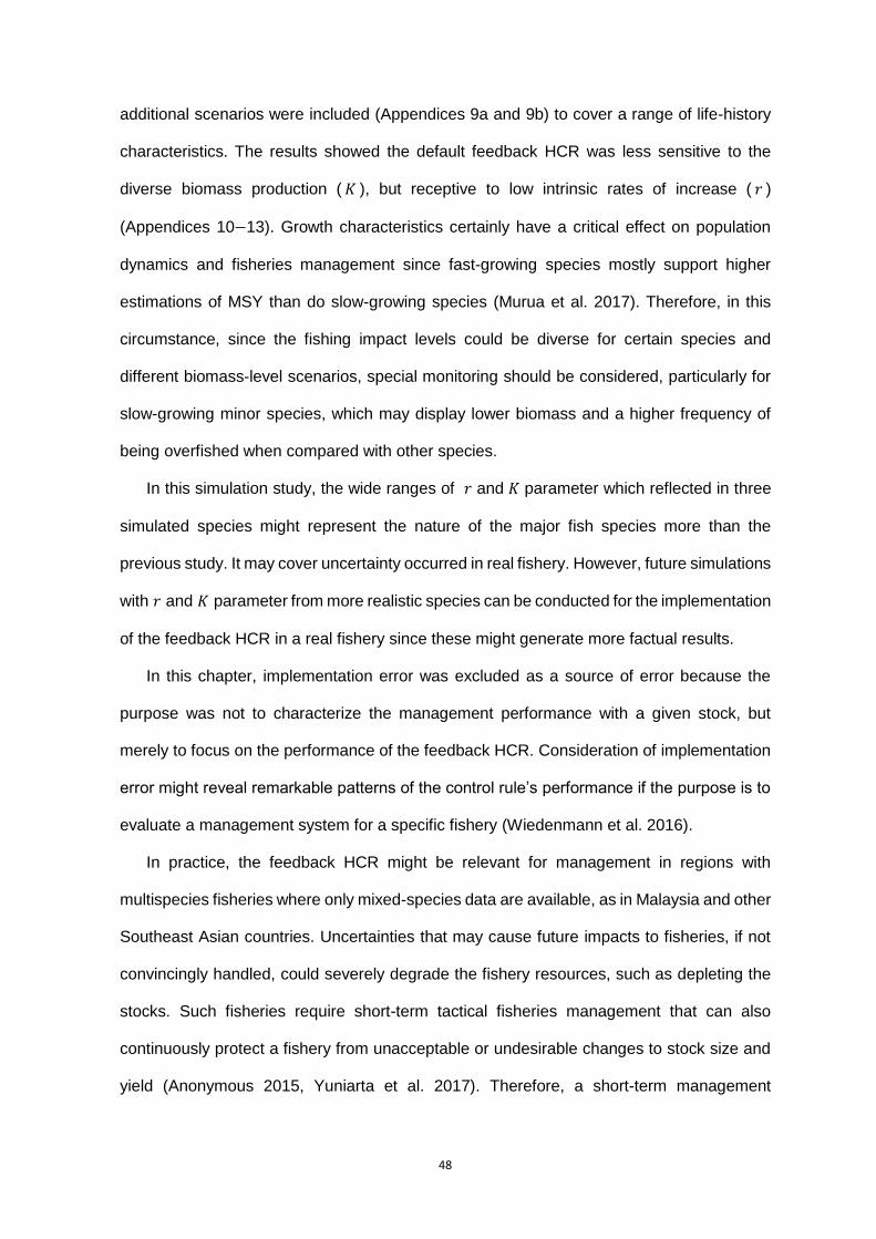
48
additional scenarios were included (Appendices 9a and 9b) to cover a range of life-history
characteristics. The results showed the default feedback HCR was less sensitive to the
diverse biomass production ( 𝐾 ), but receptive to low intrinsic rates of increase ( 𝑟 )
(Appendices 10−13). Growth characteristics certainly have a critical effect on population
dynamics and fisheries management since fast-growing species mostly support higher
estimations of MSY than do slow-growing species (Murua et al. 2017). Therefore, in this
circumstance, since the fishing impact levels could be diverse for certain species and
different biomass-level scenarios, special monitoring should be considered, particularly for
slow-growing minor species, which may display lower biomass and a higher frequency of
being overfished when compared with other species.
In this simulation study, the wide ranges of 𝑟 and 𝐾 parameter which reflected in three
simulated species might represent the nature of the major fish species more than the
previous study. It may cover uncertainty occurred in real fishery. However, future simulations
with 𝑟 and 𝐾 parameter from more realistic species can be conducted for the implementation
of the feedback HCR in a real fishery since these might generate more factual results.
In this chapter, implementation error was excluded as a source of error because the
purpose was not to characterize the management performance with a given stock, but
merely to focus on the performance of the feedback HCR. Consideration of implementation
error might reveal remarkable patterns of the control rule’s performance if the purpose is to
evaluate a management system for a specific fishery (Wiedenmann et al. 2016).
In practice, the feedback HCR might be relevant for management in regions with
multispecies fisheries where only mixed-species data are available, as in Malaysia and other
Southeast Asian countries. Uncertainties that may cause future impacts to fisheries, if not
convincingly handled, could severely degrade the fishery resources, such as depleting the
stocks. Such fisheries require short-term tactical fisheries management that can also
continuously protect a fishery from unacceptable or undesirable changes to stock size and
yield (Anonymous 2015, Yuniarta et al. 2017). Therefore, a short-term management

49
approach, such as the feedback HCR can technically respond to the demands of data-limited
management.
Particular HCRs (reviewed in Deroba and Bence 2008) have specific functions, such as
maximizing yield or profits, minimizing the risk of overexploitation by maintaining biomass
above the MSY threshold, minimizing the stock’s recovery time, or minimizing the variability
of the yield and profits. Accordingly, this feedback HCR might not be credited as an optimal
harvest policy for some data-limited fisheries as compared with some HCRs already
reviewed in other studies (Wiedenmann 2013, Carruthers et al. 2014, Dowling et al. 2015a,
Newman et al. 2015). However, the feedback HCR described here presents an initial step
toward sustainably managing multispecies fisheries while contending with data-limited
conditions. Accordingly, Malaysia and other SEA countries are still able to manage their
fishery resource sustainably by strictly limiting fishing exploitation on target species while
progressively improving their fishery data collection. Afterwards, future improvements to
species-specific data availability will allow application of more sophisticated and optimal
HCRs. The results of this chapter may be used as a simulation-based reference to expand
the use of the default feedback HCR to handle not only single-species fisheries but also
mixed-species fisheries.

50
4. GENERAL CONCLUSIONS
The current fisheries management in Malaysia has been concentrated into the National
Plan of Action for the Management of Fishing Capacity (NPOA Fishing Capacity) Plan 2
2015 which shows the fulfillment of Malaysia’s commitment to The Food and Agriculture
Organization (FAO) Code of Conduct for Responsible Fishing (CCRF) and FAO
International Plan of Action for the Management of Fishing Capacity (IPOA-Capacity). The
NPOA document addresses the imbalance between the number of fishing vessels and the
standing stocks and emphasizes enhancing monitoring and evaluation as actions to manage
fishing capacity. The main goal of the NPOA Fishing Capacity 2015 was to achieve an
efficient, equitable and transparent management of fishing capacity in marine capture
fisheries by 2018. According to the document, Malaysia needs to commit to maintaining
sustainable fisheries to accomplish FAO’s directives (DOF Malaysia 2015, Harlyan and
Matsuishi 2017, Jamaludin et al. 2017) by applying multiple measures that include input and
output controls.
In regard to input control implementation, Malaysia has reduced the number of vessels
for all types and gears based on MSY level, while conducting regular assessments on the
level of fishing capacity and evaluating the status of fishery resources. Fisheries
management in Malaysia is based on the MSY level as a product of the conventional single-
species stock assessment model. The model requires data from each species (Hilborn and
Walters 1992, Shertzer and Williams 2008, Newman et al. 2018). Otherwise, it will lead to
failures in adjustment on fishing capacity and assessment on the status of fish stocks due
to unavailability on species-separated data. But, in Malaysia and other Southeast Asian
countries, multispecies fisheries can provide only mixed-data. Therefore, assessment of the
current MSY calculation and analyses is needed for future fisheries management.
For other input control implementation, for many years, a moratorium on vessels and
gear give the impression that DoF is willing to increase the numbers of larger vessels (>70
GRT vessels) than the numbers of smaller vessels (<70 GRT vessels). This is because there

51
has been a strict moratorium on issuances of smaller vessels, while increasing issuances of
issuing larger-vessel licenses, as the Government’s policy to improve the capacity of vessels.
The Government might reduce the number of vessels but continue to increase the fishing
capacity by allowing larger vessels to operate more. In some cases, the fishing effort could
remain relatively constant over time, such as number of nets, number of fishing days, while
the increase of size of nets and total engine power of fishing vessels might substantially
increase fishing capacity (Rahikainen and Kuikka 2002, Chae and Pascoe 2005, McCluskey
and Lewison 2008).
In practice, license renewal for larger vessels seems to encourage fishers to land more
fish as fishers must declare 350 tons of landings per year, which conflicts with the mandate
of NPOA Fishing Capacity to preserve standing stocks towards the increase of fishing
capacity. Filling in fishing logbooks (LOV) is necessary to provide information concerning
the quantities caught and fishing zones (Duzgunes and Saglam 2008), which is critical to
ensure traceability and to control transshipment (Morgan et al. 2007). Besides, the
declaration of landings also improve the landing information of larger vessels, which can
significantly affect fisheries management in Malaysia, in particular for improving fish stock
assessment. However, setting the declaration of landings at a large amount will promote
increasing fishing pressures on Malaysian waters. Therefore, it is strongly suggested to
continue putting the declaration of landing, without setting a landing quota as a requirement
for vessel license renewal.
In addition, to strengthen MCS capacity and capability, several programs are planned to
systematically improve cooperation at regional levels, such as regional coordination
meetings and joint surveillance with neighboring countries. However, these purposes seem
to conflict with one requirement for getting vessel license renewals, which is to declare at
least 80% of fishing monitoring tracking unit in Malaysian waters. This means that up to 20%
would be in the EEZ of neighboring countries, which could lead to regional conflict to
bordered countries.

52
Most fishers understand these situations and avoid southern areas near the border with
Indonesia and concentrated fishing effort in northern areas (Forbes 2014). Indonesia has
declared its national sovereignty over fisheries resources in its EEZ. The Indonesian
government has strictly dealt with foreign illegal, unreported and unregulated (IUU) fishing
since 2012 (McIlgorm and Campbell 2018). This has occurred because there are no
international waters in this region.
The fact that multispecies fisheries that cannot provide species-separated data has lead
Malaysia to rely on the previous management strategies conducted. Yet Malaysia remains
still experiences excessive fishing capacity (Pascoe and Greboval 2003, Department of
Fisheries Malaysia 2015), which can be solved by output control measures (FAO 2009),
such as implementation of IQS.
Before implementing the IQS, managers must determine either single- or multi- species
approach. For tropical countries, such as Malaysia and other SEA countries, to implement
an output control, they should take a measure that can straightforwardly allow their mixed-
species data. A validated default feedback HCR can be an option of other HCRs.
To determine the possibility of the default feedback HCR implementation in the purse
seine fishery in Malaysia, some possible benefits and challenges need to be considered.
Some benefits might be attained particularly in regard to data-limited situations. One of
management objectives to obtain sustainable fisheries that have optimum catch and
biomass along with less catch variation might be accomplished. Other benefits are related
to the role of the default feedback HCR as output control measure to directly restrict the
fleets from the certain target stocks. For slow-growing species, if Malaysian fisheries are
capable of providing species-separated data, separate management should be considered
by performing special monitoring along with assessment using the modified feedback HCR.
However, some challenges might arise in the implementation of feedback HCR. In some
cases, introducing output control in the fishery where fishers familiar more with input control
might lead to some confusion among the fishery stakeholders. Fishers will consider using
their fishing licenses to catch as many fish as they can with no consideration of quota that

53
will be produced from output control measures. Other problems might also arise from
stakeholders and their interests, since too many licensed vessels operated previously need
to be operated to get more fish, which contradicts with the purpose of output control to limit
the exploitation of certain fish stocks.
There are some other important management approaches related to future purse seine
management. Short-term management approaches should focus on maintaining
multispecies fisheries with mixed-species data by feedback HCR. The feedback HCR might
be one management measure until improvements on species-specific data are available.
Therefore, in the long-term approach, applications of more sophisticated and optimum HCRs
might be promoted under species-separated data support systems.
The current management zones in SEA fisheries are applied fishing zones as a spatial
management tool to restrict fishing in certain areas, which is based on distance from shore.
This tool seems to be inconsistent with the assemblage patterns observed. (Garces et al.
2006). Therefore, it is suggested to re-structure the management by taking into account the
basic pattern of the fish assemblages.
Malaysian fisheries and other fisheries in SEA have similar characteristics and
sustainability issues. Therefore, compiling a set of management measures for Malaysian
fisheries can be used in other SEA countries. SEA might improve input control
implementation by limiting fishing effort, but for some cases, it will not solve imbalance
between the amount of effort and the standing stock, since it will not protect the stocks from
gears. On the other hand, implementing output control solely will lead to critical fishery
conflicts since fishers will compete to land the limited quotas. The fishers will race to fish by
allocating all their effort to get more fish, which will lead to other fishery sustainability issues
such as over-investment. Therefore, a combination of input and output controls will be the
best option for providing sustainable fisheries management for Malaysian fisheries and other
multispecies fisheries in the region. Concerning Malaysian multispecies fisheries, applying
the feedback HCR might be a short management approach before implementing the IQS,
which later will complete their multiple measures for sustainable fisheries.

54
This research pointedly suggests that data-limited multispecies fisheries can be
managed sustainably by using multiple management measures, such as a combination of
input, output and technical controls. However, it still must be cautioned that improvement on
species-specific data availability for the major species or depleted species should be one of
the main multispecies fishery issues to be solved in the near future. The availability of
reliable species-specific data for certain major species and mixed-species data for other
species will generate substantial progress for fisheries management in SEA.

55
REFERENCES
Abdi, H. and Williams, L.J. 2010. Principal component analysis. Wiley Interdiscip. Rev. Comput. Stat. 2(4): 433–459. doi:10.1002/wics.101
Abdussamad, E., Pillai, N.G.K., Kasim, H.M., Habeeb, O.M.M.J., And, M., and Jeyabalan, K. 2010. Fishery, biology and population characteristics of the Indian mackerel, Rastrelliger kanagurta (Cuvier) exploited along the Tuticorin coast. Indian J. Fish. 57: 17–21.
Amornpiyakrit, T. and Siriraksophon, S. 2016. Management of fishing capacity for sustainable fisheries: RPOA-Capacity. Fish people 14(2): 18–23. Available from http://hdl.handle.net/20.500.12066/991
Anderson, C.M., Krigbaum, M.J., Arostegui, M.C., Feddern, M.L., Koehn, J.Z., Kuriyama, P.T., Morrisett, C., Akselrud, C.I.A., Davis, M.J., Fiamengo, C., Fuller, A., Lee, Q., McElroy, K.N., Pons, M., and Sanders, J. 2018. How commercial fishing effort is managed. Fish Fish. doi:10.1111/faf.12339
Anonymous. 2015, October. Marine Fisheries Management Plan of Thailand: A National Policy for Marine Fisheries Management (2015–2019). Department of Fisheries Ministry of Agriculture and Cooperatives, Thailand.
Arreguín-Sánchez, F. 1996. Catchability: a key parameter for fish stock assessment. Rev. Fish Biol. Fish. 6(2): 221–242. doi:10.1007/BF00182344
Baudron, A., Ulrich, C., Nielsen, J.R., and Boje, J. 2010. Comparative evaluation of a mixed-fisheries effort-management system based on the Faroe Islands example. ICES J. Mar. Sci. 67(5): 1036–1050. doi:10.1093/icesjms/fsp284
Boyle, K., Kaiser, M., S, T., Murray, L., and Duncan, P. 2016. Spatial variation in fish and invertebrate bycatches in a scallop trawl fishery. In Journal of Shellfish Research. doi:10.2983/035.035.0102
Butterworth, D.S. 2007. Why a management procedure approach? Some positives and negatives. ICES J. Mar. Sci. 64(4): 613–617. doi:10.1093/icesjms/fsm003
Cadrin, S.X. and Dickey-Collas, M. 2015. Stock assessment methods for sustainable fisheries. ICES J. Mar. Sci. 72(1): 1–6. doi:10.1093/icesjms/fsu228
Carruthers, T.R., Punt, A.E., Walters, C.J., MacCall, A., McAllister, M.K., Dick, E.J., and Cope, J. 2014. Evaluating methods for setting catch limits in data-limited fisheries. Fish. Res. 153: 48–68. doi:10.1016/j.fishres.2013.12.014
Chae, D.-R. and Pascoe, S. 2005. Use of simple bioeconomic models to estimate optimal effort levels in the Korean coastal flounder fisheries. Aquat. Living Resour. 18(2): 93–101. doi:10.1051/alr:2005012
Chee, P. 1995. Tuna fisheries interactions in Malaysia. In Proceedings of the second FAO Expert Consultation Interactions of Pacific Tuna Fisheries. Edited by R. Shomura, J. Majkowski, and R. Harman. Shimizu, Japan. p. 612.
Chuenpagdee, R., Morgan, L.E., Maxwell, S.M., Norse, E.A., and Pauly, D. 2003. Shifting gears: assessing collateral impacts of fishing methods in US waters. Front. Ecol. Environ. 1(10): 517–524. doi:10.1890/1540-9295(2003)001[0517:SGACIO]2.0.CO;2
Chumchuen, W., Matsuoka, T., Anraku, K., and Arnupapboon, S. 2016. Size-selective catch in tropical tuna purse seine fishery in the Eastern Indian Ocean: Assessment on

56
new selectivity model for purse seine net. Fish. Sci. 82(3): 391–404. doi:10.1007/s12562-016-0977-9
Cochrane, K.L. 2002. A fishery manager’s guidebook. Management measures and their application. In FAO. Fisheries Technical Paper. doi:10.1017/CBO9781107415324.004
Collette, B., Di Natale, A., Fox, W., Juan-Jordá, M.J., Miyabe, M., Nelson, R., Sun, C., and Uozomi, Y. 2011. Thunnus tonggol. The IUCN Red List of Threatened Species 2011: e.T170351A6763691. doi:10.2305/IUCN.UK.2011-2.RLTS.T170351A6763691.en
Corbett, J. and Keller, P. 2006. Using community information systems to communicate traditional knowledge embedded in the landscape. Particip. Learn. Action 54(April): 1–154.
Costanza, R. and Patten, B.C. 1995. Defining and predicting sustainability. Ecol. Econ. 15(3): 193–196. doi:10.1016/0921-8009(95)00048-8
Department of Fisheries Malaysia. 2013. APFIC Regional expert workshop on tropical trawl fishery management. Phuket, Thailand.
Department of Fisheries Malaysia. 2015. National Plan of Action for the Management of Fishing Capacity in Malaysia (Plan 2). Putrajaya.
Department of Fisheries Malaysia year of 2002-2016. 2016. Annual Fisheries Statistics. Kuala Lumpur. Available from http://www.dof.gov.my.
Deroba, J.J. and Bence, J.R. 2008. A review of harvest policies: Understanding relative performance of control rules. Fish. Res. 94(3): 210–223. doi:10.1016/j.fishres.2008.01.003
Dichmont, C., Deng, R., Punt, A., Venables, W., and Hutton, T. 2012. From input to output controls in a short-lived species: The case of Australia’s northern prawn fishery. Mar. Freshw. Res. 63: 727–739. doi:10.1071/MF12068
DOF Malaysia. 2015. Current status of purse seine fisheries in the Southeast Asian region. Edited ByR.B.R. Hassan. Department of Fisheries Malaysia, Kuala Terengganu, Malaysia.
Dowling, N.A., Dichmont, C.M., Haddon, M., Smith, D.C., Smith, A.D.M., and Sainsbury, K. 2015a. Empirical harvest strategies for data-poor fisheries: A review of the literature. Fish. Res. 171: 141–153. doi:10.1016/j.fishres.2014.11.005
Dowling, N.A., Dichmont, C.M., Haddon, M., Smith, D.C., Smith, A.D.M., and Sainsbury, K. 2015b. Guidelines for developing formal harvest strategies for data-poor species and fisheries. Fish. Res. 171(Supplement C): 130–140. doi:10.1016/j.fishres.2014.09.013
Dunn, D., Boustany, A., and Halpin, P. 2011. Spatio-temporal management of fisheries to reduce by-catch and increase fishing selectivity. Fish Fish. doi:10.1111/j.1467-2979.2010.00388.x
Duzgunes, E. and Saglam, N. 2008. Fisheries management in the Black Sea countries. Turkish J. Fish. Aquat. Sci. 8: 181–192.
FAO. 2004. Progress on the implementation of the International Plan of Action for Management of Fishing Capacity. FAO, Rome.
FAO. 2005. Report of the FAO Regional workshop on the elaboration of national plans of

57
action to prevent, deter and eliminate illegal, unreported and unregulated fishing Southeast Asia Subregion. Penang, Malaysia, 10-14 October 2004. FAO Fisheries Report. No. 757. Rome.
FAO. 2008. 3. Managing fishing capacity. In FAO Technical Guidelines for Responsible Fisheries No 4 Suppl.3. p. 104.
FAO. 2009. Technical guidelines for responsible fisheries management. In FAO technical guidlines for responsible fisheries 4. doi:10.1017/CBO9781107415324.004
FAO. 2018. The state of World Fisheries and Aquaculture 2018 - Meeting the sustainable development goals. Rome. Licence: CC BY-NC-SA 3.0 IGO.
FAO Fisheries Department. 2003. The ecosystem approach to fisheries. In FAO Technical Guidelines for Responsible Fisheries No 4 Suppl.2. doi:10.1017/S0020818300006160
FAO Fishery Resources Division and Fishery Policy and Planning Division. 1997. Fisheries management. FAO Technical Guidelines for Responsible Fisheries. No. 4. FAO, Rome.
Fisheries Agency and Fisheries Research and Education Agency of Japan. 2017. Marine fisheries stock assessment and evaluation for Japanese waters (fiscal year 2016/2017).
Forbes, V.L. 2014. Indonesia’s delimited maritime boundaries. Edited by V.L. Forbes. Springer Berlin Heidelberg, Berlin, Heidelberg. pp. 33–63. doi:10.1007/978-3-642-54395-1_3
Fox, W.W.J. 1970. An exponential surplus-yield model for optimizing exploited fish populations. Trans. Am. Fish. Soc. 99: 80–88. doi:10.1577/1548-8659(1970)99<80:AESMFO>2.0.CO;2
Gaichas, S.K., Fogarty, M., Fay, G., Gamble, R., Lucey, S., Smith, L., and Prellezo, R. 2017. Combining stock, multispecies, and ecosystem level fishery objectives within an operational management procedure: simulations to start the conversation. ICES J. Mar. Sci. 74(2): 552–565. doi:10.1093/icesjms/fsw119
Garces, L.R., Stobutzki, I., Alias, M., Campos, W., Koongchai, N., Lachica-Alino, L., Mustafa, G., Nurhakim, S., Srinath, M., and Silvestre, G. 2006. Spatial structure of demersal fish assemblages in South and Southeast Asia and implications for fisheries management. Fish. Res. 78(2): 143–157. doi:10.1016/j.fishres.2006.02.005
Griffiths, S.P., Fry, G.C., Manson, F.J., and Lou, D.C. 2009. Age and growth of longtail tuna (Thunnus tonggol) in tropical and temperate waters of the central Indo-Pacific. ICES J. Mar. Sci. 67(1): 125–134. doi:10.1093/icesjms/fsp223
Haedrich, R.L. and Barnes, S.M. 1997. Changes over time of the size structure in an exploited shelf fish community. Fish. Res. 31(3): 229–239. doi: 10.1016/S0165-7836(97)00023-4
Harlyan, L.I. and Matsuishi, T. 2017. An overview of purse seine fisheries in Malaysia. In The JSFS 855h Anniversary-Commemorative International Symphosium “Fisheries Science for Future Generations.” Tokyo. p. 02005. Available from www.jsfs.jp.
Harlyan, L.I., Wu, D., Kinashi, R., Kaewnern, M., and Matsuishi, T. 2019. Validation of a feedback harvest control rule in data-limited conditions for managing multispecies fisheries. Can. J. Fish. Aquat. Sci. NRC Research Press. doi:10.1139/cjfas-2018-0318

58
Hassan, R.B.R. 1992. Study on the use of payao on the east coast of Peninsular Malaysia. Ministry of Agriculture, Dept. of Fisheries.
Hassan, R.B.R. and Latun, A.R. 2016. Purse seine fisheries in Southeast Asian Countries: A regional synthesis. Fish People 14(1): 7-15. Available from http://hdl.handle.net/20.500.12066/980
Hilborn, R., and Walters, C.J. (Editors). 1992. Quantitative Fisheries Stock Assessment: Choice, Dynamics and Uncertainty. Springer US.
Hiramatsu K. 2004. Evaluation of the ABC decision rule by the operating model approach. Nippon Suisan Gakkaishi 70(6): 879–883. doi:10.2331/suisan.70.879
Hoggarth, D.D., Abeyasekera, S., Arthur, R., Beddington, J.R., Burn, R.W., Halls, A., Kirkwood, G.P., McAllister, M.K., Medley, P., Mees, C., Parkes, G., Pilling, G., Wakeford, R., and Welcomme, R. 2006. Stock assessment for fishery management - A framework guide to the stock assessment tools of the Fisheries Management Science Programme (FMSP). FAO Technical Paper No.487, Rome.
Hollowed, A.B., Bax, N., Beamish, R., Collie, J., Fogarty, M., Livingston, P., Pope, J., and Rice, J.C. 2000. Are multispecies models an improvement on single-species models for measuring fishing impacts on marine ecosystems? ICES J. Mar. Sci. 57(3): 707–719. doi:10.1006/jmsc.2000.0734
Hoshino, E., Milner-Gulland, E.J., and Hillary, R.M. 2012. Bioeconomic adaptive management procedures for short-lived species: A case study of Pacific saury (Cololabis saira) and Japanese common squid (Todarodes pacificus). Fish. Res. 121–122(Supplement C): 17–30. doi:10.1016/j.fishres.2012.01.007
Hurtado-Ferro, F., Hiramatsu, K., and Shirakihara, K. 2010. Allowing for environmental effects in a management strategy evaluation for Japanese sardine. ICES J. Mar. Sci. 67(9): 2012–2017. doi:10.1093/icesjms/fsq126
Ichinokawa, M., Okamura, H., and Kurota, H. 2017. The status of Japanese fisheries relative to fisheries around the world. ICES J. Mar. Sci. 74(5): 1277–1287. doi:10.1093/icesjms/fsx002
Ichinokawa, M., Okamura, H., Kurota, H., Yukami, R., Tanaka, H., Shibata, Y., and Ohshimo, S. 2015. Searching for optimum management procedures by quantifying management objectives for Japanese domestic fishery stocks without stock biomass estimation. Nippon Suisan Gakkaishi 81(2): 206–218. doi:10.2331/suisan.81.206
Iriondo, A., García, D., Santurtún, M., Castro, J., Quincoces, I., Lehuta, S., Mahévas, S., Marchal, P., Tidd, A., and Ulrich, C. 2012. Managing mixed fisheries in the European Western Waters: Application of Fcube methodology. Fish. Res. 134–136: 6–16. doi: 10.1016/j.fishres.2012.07.019
Islam, G.M.N., Noh, K.M., Sidique, S.F., and Noh, A.F.M. 2014. Economic impact of artificial reefs: A case study of small scale fishers in Terengganu, Peninsular Malaysia. Fish. Res. 151: 122–129. doi:10.1016/j.fishres.2013.10.018
Jamaludin, N.A., Saleh, M.F.M., Hassan, R.B.R., and Fatah, N.N.A. 2017. The 3rd Core expert meeting on “Comparative Studies for management of purse seine fisheries in the Southeast Asian region”: 12 - 14 September 2017. Kuala Lumpur, Malaysia.
Jardim, E., Azevedo, M., and Brites, N.M. 2015. Harvest control rules for data limited stocks using length-based reference points and survey biomass indices. Fish. Res. 171(Supplement C): 12–19. doi:10.1016/j.fishres.2014.11.013

59
Jenkins, C.N. and van Houtan, K.S. 2016. Global and regional priorities for marine biodiversity protection. Biol. Conserv. 204: 333–339. doi:10.1016/j.biocon.2016.10.005
Jennings, S., Alvsvåg, J., Cotter, A.J.R., Ehrich, S., Greenstreet, S.P.R., Jarre-Teichmann, A., Mergardt, N., Rijnsdorp, A.D., and Smedstad, O. 1999. Fishing effects in northeast Atlantic shelf seas: patterns in fishing effort, diversity and community structure. III. International trawling effort in the North Sea: an analysis of spatial and temporal trends. Fish. Res. 40(2): 125–134. doi:10.1016/S0165-7836(98)00208-2
Johannes, R.E. 1998. The case for data-less marine resource management: examples from tropical nearshore finfisheries. Trends Ecol. Evol. 13(6): 243–246. doi:10.1016/S0169-5347(98)01384-6
Jul-Larsen, E., Kolding, J., Overå, R., Nielsen, J.R., and Zwieten, P.A.M. 2003. Management, co-management or no management? Major dillemas in southern African freshwater fisheries. 1. Synthesis report. In FAO Fisheries Technical Paper. No. 426/1. Rome.
Kato, Y. 2008. Steering the small-scale fisheries of Southeast Asia towards responsible development. Fish People 6(1): 3–9. Available from http://hdl.handle.net/20.500.12066/753
Kindt-Larsen, L., Kirkegaard, E., and Dalskov, J. 2011. Fully documented fishery: a tool to support a catch quota management system. ICES J. Mar. Sci. 68(8): 1606–1610. doi:10.1093/icesjms/fsr065
Kirkley, J.E., Ishak, H.O., Alam, M.F., and Squires, D. 2003. Excess capacity and asymmetric information in developing country fisheries: The Malaysian Purse Seine Fishery. Am. J. Agric. Econ. 85(3): 647–662. doi:10.1111/1467-8276.00462
Kleisner, K., Zeller, D., Froese, R., and Pauly, D. 2013. Using global catch data for inferences on the world’s marine fisheries. Fish Fish. 14(3): 293–311. doi:10.1111/j.1467-2979.2012.00469.x
Klemas, V. 2013. Fisheries applications of remote sensing: An overview. Fish. Res. 148(May 2014): 124–136. doi:10.1016/j.fishres.2012.02.027
Kolody, D. and Jumppanen, P. 2018. Indian Ocean skipjack purse seine catchability trends estimated from bigeye and yellowfin assessments. Available from http://www.iotc.org/documents/WPTT/20/32
Kvamsdal, S.F., Eide, A., Ekerhovd, N.-A., Enberg, K., Gudmundsdottir, A., Hoel, A.H., Mills, K.E., Mueter, F.J., Ravn-Jonsen, L., Sandal, L.K., Stiansen, J.E., and Vestergaard, N. 2016. Harvest control rules in modern fisheries management. Elem Sci Anth 4(0). doi:10.12952/journal.elementa.000114
Le, S., Josse, J., and Husson, F. 2008. FactoMineR: An R Package for Multivariate Analysis. J. Stat. Softw. 25(1): 1–18. doi:10.18637/jss.v025.i01
Lipps, J.H., Berger, W.H., Buzas, M.A., Dauglas, R.G., Ross, C.A., and Buzas, M.A. 2014. The Measurement of Species Diversity. Foraminifer. Ecol. Paleocology: 3–10. doi:10.2110/scn.79.06.0003
Mace, P.M. 2001. A new role for MSY in single-species and ecosystem approaches to fisheries stock assessment and management. Fish Fish. 2(1): 2–32. doi:10.1046/j.1467-2979.2001.00033.x

60
Macusi, E.D., Abreo, N.A.S., and Babaran, R.P. 2017. Local ecological knowledge (LEK) on fish behavior around anchored FADs: The case of tuna purse seine and ringnet fishers from southern Philippines. doi:10.3389/fmars.2017.00188
Maechler, M., Rousseeuw, P., Struyf, A., Hubert, M., and Hornik, K. 2018. cluster: Cluster Analysis Basic and Extensions. R Package version 2.0.7-1.
Magnusson, K.G. 1992. A feedback and probing strategy to regulate harvesting from a renewable resource. Math. Med. Biol. 9: 43–65. doi:10.1093/imammb/9.1.43
Makino, M. 2011. Fisheries management in Japan. In 1st edition. Springer, Japan. doi:10.1007/978-94-007-1777-0
Marchal, P., Andersen, J.L., Aranda, M., Fitzpatrick, M., Goti, L., Guyader, O., Haraldsson, G., Hatcher, A., Hegland, T.J., Le Floc’h, P., Macher, C., Malvarosa, L., Maravelias, C.D., Mardle, S., Murillas, A., Nielsen, J.R., Sabatella, R., Smith, A.D.M., Stokes, K., Thoegersen, T., and Ulrich, C. 2016. A comparative review of fisheries management experiences in the European Union and in other countries worldwide: Iceland, Australia, and New Zealand. Fish Fish. 17(3): 803–824. doi:10.1111/faf.12147
Matsuda, H., Makino, M., Tomiyama, M., Gelcich, S., and Castilla, J.C. 2010. Fishery management in Japan. Ecol. Res. 25(5): 899–907. doi:10.1007/s11284-010-0748-5
Maunder, M.N., Sibert, J.R., Fonteneau, A., Hampton, J., Kleiber, P., and Harley, S.J. 2006. Interpreting catch per unit effort data to assess the status of individual stocks and communities. ICES J. Mar. Sci. 63(8): 1373–1385. doi:10.1016/j.icesjms.2006.05.008
McCluskey, S.M. and Lewison, R.L. 2008. Quantifying fishing effort: a synthesis of current methods and their applications. Fish Fish. 9(2): 188–200. doi:10.1111/j.1467-2979.2008.00283.x
McIlgorm, A. and Campbell, B. 2018. Future Opportunities and Challenges in Developing Sustainable Offshore Indonesian Fisheries. Brill, Leiden, The Netherlands. pp. 66–80. doi:10.1163/9789004366619_009
Möllmann, C., Lindegren, M., Blenckner, T., Bergström, L., Casini, M., Diekmann, R., Flinkman, J., Müller-Karulis, B., Neuenfeldt, S., Schmidt, J.O., Tomczak, M., Voss, R., and Gårdmark, A. 2014. Implementing ecosystem-based fisheries management: from single-species to integrated ecosystem assessment and advice for Baltic Sea fish stocks. ICES J. Mar. Sci. 71(5): 1187–1197. doi:10.1093/icesjms/fst123
Morgan, G., Staples, D., and Funge-Smith, S. 2007. Fishing capacity management and IUU fishing in Asia. FAO, Bangkok.
Morison, A.K. 2004. Input and output controls in fisheries management: a plea for more consistency in terminology. Fish. Manag. Ecol. 11(6): 411–413. doi:10.1111/j.1365-2400.2004.00414.x
Murawski, S. 1991. Can we Manage manage our multispecies fisheries? Fisheries 16(5): 5–13. doi:10.1577/1548-8446(1991)016<0005:CWMOMF>2.0.CO;2
Murawski, S., M. Lange, A., Sissenwine, M., and K. Mayo, R. 1983. Definition and Analysis of Multispecies Otter-Trawl Fisheries Off the Northeast Coast of the United-States. ICES J. Mar. Sci. 41: 13–27. doi:10.1093/icesjms/41.1.13
Murua, H., Rodriguez-Marin, E., Neilson, J.D., Farley, J.H., and Juan-Jordá, M.J. 2017. Fast versus slow growing tuna species: age, growth, and implications for population

61
dynamics and fisheries management. Rev. Fish Biol. Fish. 27(4): 733–773. doi:10.1007/s11160-017-9474-1
Navarrete Forero, G., Miñarro, S., Mildenberger, T.K., Breckwoldt, A., Sudirman, and Reuter, H. 2017. Participatory Boat Tracking Reveals Spatial Fishing Patterns in an Indonesian Artisanal Fishery. doi:10.3389/fmars.2017.00409
Newman, D., Berkson, J., and Suatoni, L. 2015. Current methods for setting catch limits for data-limited fish stocks in the United States. Fish. Res. 164: 86–93. doi:10.1016/j.fishres.2014.10.018
Newman, S.J., Brown, J.I., Fairclough, D. V., Wise, B.S., Bellchambers, L.M., Molony, B.W., Lenanton, R.C.J., Jackson, G., Smith, K.A., Gaughan, D.J., Fletcher, W. (Rick) J., McAuley, R.B., and Wakefield, C.B. 2018. A risk assessment and prioritisation approach to the selection of indicator species for the assessment of multi-species, multi-gear, multi-sector fishery resources. Mar. Policy 88(Supplement C): 11–22. doi:10.1016/j.marpol.2017.10.028
Ohshimo, S. and Naya, M. 2014. Management strategy evaluation of fisheries resources in data-poor situations using an operating model based on a production model. Japan Agric. Res. Q. JARQ 48(2): 237–244. doi:10.6090/jarq.48.237
Oksanen, J., Blanchet, F.G., Friendly, M., Kindt, R., Legendre, P., McGlinn, D., Minchin, P.R., R.B., O., Simpson, G.L., Solymos, P., Stenvens, M.H.H., Szoecs, E., and Wagner, H. 2018. Vegan: Community Ecology Package. Available from https://cran.r-project.org/package=vegan
De Oliveira, J.A.A., Kell, L.T., Punt, A., Roel, B.A., and Butterworth, D.S. 2008. Managing without best predictions: The management strategy evaluation framework. In Advances in Fisheries Science. Edited by A. Payne, J. Cotter, and T. Potter. Blackwell Publishing Ltd., Oxford, UK. pp. 104–134.
Parravicini, V., Kulbicki, M., Bellwood, D.R., Friedlander, A.M., Arias-Gonzalez, J.E., Chabanet, P., Floeter, S.R., Myers, R., Vigliola, L., D’Agata, S., and Mouillot, D. 2013. Global patterns and predictors of tropical reef fish species richness. Ecography (Cop.). 36(12): 1254–1262. doi:10.1111/j.1600-0587.2013.00291.x
Pascoe, S. and Greboval, D. 2003. Measuring capacity in fisheries. In FAO. Fisheries Technical Paper. doi:10.1016/j.arabjc.2015.02.024
Peet, R.K. 1974. The measurement of species diversity. Source Annu. Rev. Ecol. Syst. 5244: 285–307. doi:10.1146/annurev.es.05.110174.001441 Pomeroy, R.S. 1995. Community-based and co-management institutions for sustainable coastal fisheries. Ocean Coast. Manag. 27: 143–162. doi:10.1016/0964-5691(95)00042-9
Pomeroy, R.S. 2012. Managing overcapacity in small-scale fisheries in Southeast Asia. Mar. Policy 36(2): 520–527. doi:10.1016/j.marpol.2011.10.002
Punt, A.E. 2010. Harvest control rules and fisheries management. In Handbook of Marine Fisheries Conservation and Management. Edited by R.Q. Grafton, R. Hilborn, D. Squires, M. Tait, and M. Williams. Oxford University Press, Oxford, New York. pp. 582–594.
Punt, A.E., Butterworth, D.S., Moor, C.L., Oliveira, D., A, J.A., and Haddon, M. 2016. Management strategy evaluation: best practices. Fish Fish. 17(2): 303–334. doi:10.1111/faf.12104
Punt, A.E., Dorn, M.W., and Haltuch, M.A. 2008. Evaluation of threshold management
62
strategies for groundfish off the U.S. West Coast. Fish. Res. 94(3): 251–266. doi:10.1016/j.fishres.2007.12.008
Purcell, S.W. and Pomeroy, R.S. 2015. Driving small-scale fisheries in developing countries. Available from https://www.frontiersin.org/article/10.3389/fmars.2015.00044
QGIS Development Team. 2009. QGIS Geographic Information System. Open Source Geospatial Foundation. Available from http://qgis.org.
Qiu, Y., Lin, Z., and Wang, Y. 2010. Responses of fish production to fishing and climate variability in the northern South China Sea. Prog. Oceanogr. 85(3): 197–212. doi: 10.1016/j.pocean.2010.02.011
R Core Team. 2018. R: A Language and Environment for Statistical Computing. R Foundation for Statistical Computing, Vienna, Austria. Available from https://www.r-project.org/
Rahikainen, M. and Kuikka, S. 2002. Fleet dynamics of herring trawlers—change in gear size and implications for interpretation of catch per unit effort. Can. J. Fish. Aquat. Sci. 59(3): 531–541. NRC Research Press. doi:10.1139/f02-030
Roberts, C.M., Hawkins, J.P., and Gell, F.R. 2005. The role of marine reserves in achieving sustainable fisheries. Philos. Trans. R. Soc. Lond. B. Biol. Sci. 360(1453): 123–132. The Royal Society. doi:10.1098/rstb.2004.1578
Roy, K., Kar, S., and Das, R.N. 2015. Chapter 6 - Selected Statistical Methods in QSAR. In Understanding the Basics of QSAR for Applications in Pharmaceutical Sciences and Risk Assessment. Edited by K. Roy, S. Kar, and R.N.B.T.-U. the B. of Q. for A. in P.S. and R.A. Das. Academic Press, Boston. pp. 191–229. doi:10.1016/B978-0-12-801505-6.00006-5
Rudd, M.B. and Branch, T.A. 2017. Does unreported catch lead to overfishing? Fish Fish. 18(2): 313–323. doi:10.1111/faf.12181
Salas, S., Chuenpagdee, R., Seijo, J.C., and Charles, A. 2007. Challenges in the assessment and management of small-scale fisheries in Latin America and the Caribbean. Fish. Res. 87(1): 5–16. doi:10.1016/j.fishres.2007.06.015
Schaefer, M. 1954. Some aspects of dynamics of populations important to the management of commercial marine fisheries. Inter-American Trop. Tuna Comm. Bull. 1(2): 23–56. doi:10.1007/BF02464432
SEAFDEC. 2015a. Fishery Statistical Bulletin of Southeast Asia. Southeast Asian Fisheries Development Center, Bangkok, Thailand.
SEAFDEC. 2015b. Regional Plan of Action on Sustainable Utilization of Neritic Tunas in the ASEAN Region. Southeast Asian Fisheries Development Center, Bangkok, Thailand.
SEAFDEC. 2017. ASEAN Regional Plan of Action for the Management of Fishing Capacity (RPOA-Capacity). Southeast Asian Fisheries Development Center, Bangkok, Thailand.
Selig, E.R., Kleisner, K.M., Ahoobim, O., Arocha, F., Cruz-Trinidad, A., Fujita, R., Hara, M., Katz, L., McConney, P., Ratner, B.D., Saavedra-Díaz, L.M., Schwarz, A.-M., Thiao, D., Torell, E., Troëng, S., and Villasante, S. 2017. A typology of fisheries management tools: using experience to catalyse greater success. Fish Fish. 18(3): 543–570. doi:10.1111/faf.12192

63
Shertzer, K.W. and Williams, E.W. 2008. Fish assemblages and indicator species: reef fishes off the southeastern United States. Fish. Bull. 106(3): 257–269.
Silapajarn, K., Ishii, K., Sulit, V.T., Siriraksophon, S., and Tongdee, N. 2015. Strengthening Regional Cooperation for Sustainable Fisheries Development in Southeast Asia. Fish People 14(3): 2–11. Available from http://hdl.handle.net/20.500.12066/1002
Siriraksophon, S. 2017. Sustainable management of neritic tunas in Southeast Asia : longtail tuna and kawakawa in focus. Fish People 15(2): 14–20. Available from http://hdl.handle.net/20.500.12066/1196
Smith-Vaniz, W.. 1984. Western Indian Ocean fishing area 51. In FAO species identification sheets for fishery purposes., Vol 1. Edited by W. Fischer and G. Bianchi. Food and Agriculture Organization of the United Nations, Rome.
Sparre, P. and Venema, S.C. 1992. Introduction to tropical fish stock assessment. Part 1: manual. In FAO Fisheries Technical Paper. No. 306/1. Rev. 1. Rome.
Squires, D. and Vestergaard, N. 2015. Productivity growth, catchability, stock assessments, and optimum renewable resource use. Mar. Policy 62: 309–317. doi:10.1016/j.marpol.2015.07.006
Stefansson, G. and Rosenberg, A.A. 2005. Combining control measures for more effective management of fisheries under uncertainty: quotas, effort limitation and protected areas. Philos. Trans. R. Soc. Lond. B. Biol. Sci. 360(1453): 133–146. The Royal Society. doi:10.1098/rstb.2004.1579
Sumaila, U.R., Bellmann, C., and Tipping, A. 2016. Fishing for the future: An overview of challenges and opportunities. Mar. Policy 69: 173–180. doi:10.1016/j.marpol.2016.01.003
Suuronen, P., Chopin, F., Glass, C., Løkkeborg, S., Matsushita, Y., Queirolo, D., and Rihan, D. 2012. Low impact and fuel efficient fishing—Looking beyond the horizon. Fish. Res. 119–120: 135–146. doi:10.1016/j.fishres.2011.12.009
Suzuki, R. and Shimodaira, H. 2017. pvclust: An R package for hierarchical clustering with p-values. Available from http://stat.sys.i.kyoto-u.ac.jp/prog/pvclust/#download
Tanaka, S. 1980. A theoretical consideration on the management of a stock-fishery system by catch quota and on its dynamical properties. Nippon Suisan Gakkaishi 46(12): 1477–1482. doi:10.2331/suisan.46.1477
Welcomme, R.L. 1999. A review of a model for qualitative evaluation of exploitation levels in multi-species fisheries. Fish. Manag. Ecol. 6(1): 1–19. doi:10.1046/j.1365-2400.1999.00137.x
Wiedenmann, J. 2013. An evaluation of harvest control rules for data-poor fisheries. North Am. J. Fish. Manag. 33(4): 845–860. doi:10.1080/02755947.2013.811128
Wiedenmann, J., Wilberg, M., Sylvia, A., and Miller, T. 2016. An evaluation of acceptable biological catch (ABC) harvest control rules designed to limit overfishing. Can. J. Fish. Aquat. Sci. 74(7): 1028–1040. doi:10.1139/cjfas-2016-0381
Willette, D.A., Santos, M.D., and Leadbitter, D. 2016. Longtail tuna Thunnus tonggol (Bleeker, 1851) shows genetic partitioning across, but not within, basins of the Indo-Pacific based on mitochondrial DNA. J. Appl. Ichthyol. 32(2): 318–323. doi:10.1111/jai.12991

64
Worm, B., Hilborn, R., Baum, J.K., Branch, T.A., Collie, J.S., Costello, C., Fogarty, M.J., Fulton, E.A., Hutchings, J.A., Jennings, S., Jensen, O.P., Lotze, H.K., Mace, P.M., McClanahan, T.R., Minto, C., Palumbi, S.R., Parma, A.M., Ricard, D., Rosenberg, A.A., Watson, R., and Zeller, D. 2009. Rebuilding global fisheries. Science. 325(5940): 578–585. doi:10.1126/science.1173146
Yamakawa, T., Matsumiya, Y., Nishimura, M., and Ohnishi, S. 1994. Expanded DeLury’s method with variable catchability and its application to catch-effort data from spiny lobster gillnet fishery. Fish. Sci. 60(1): 59–63. doi:10.2331/fishsci.60.59
Yami, B.M. 1994. Purse seining manual. In 1st edition. Wiley-Blackwell.
De Young, C. 2006. Review of the state of world marine capture fisheries management: Indian Ocean. FAO Techical Paper No 458. doi:10.1108/EL-11-2011-0159
Yuniarta, S., van Zwieten, P.A.M., Groeneveld, R.A., Wisudo, S.H., and van Ierland, E.C. 2017. Uncertainty in catch and effort data of small- and medium-scale tuna fisheries in Indonesia: Sources, operational causes and magnitude. Fish. Res. 193: 173–183. doi:10.1016/j.fishres.2017.04.009
Zheng, J., and Walters, C.J. 1988. Population dynamics and stock assessment of Wanshan Spring Decapterus maruadsi (T. & S.) in South China Sea. Fish. Res. 6(3): 217–231. doi:10.1016/0165-7836(88)90015-X
Zhu, J., Dai, X., and Chen, Y. 2011. Species composition and diversity of pelagic fishes based on a longline fishery catch in the North Pacific Ocean. Chinese J. Oceanol. Limnol. 29: 261–269. doi:10.1007/s00343-011-012

65
TABLES

66
Table 1. Fishing zonation in Malaysian fisheries
Category Zone A (No-take zone)
Zone B Zone C Zone C2
Zone C3
Purpose Marine Park (Only artisanal fisheries allowed)
Commercial fisheries (Trawlers and Purse seiners)
Commercial fisheries (Trawlers and Purse seiners
Commercial fisheries (Trawlers and Purse seiners
Commercial fisheries (Tuna long liners and tuna purse seiners
Ownership Must be on board (one person owns one vessel)
Does not have to be in the vessel
Does not have to be in the vessel
Does not have to be in the vessel
Does not have to be in the vessel
Vessel size <40 GRT <40 GRT 40−<70 GRT >70 GRT >70 GRT
Fishing area (distance from shore)
0-5 nm 5-12 nm 12-30 nm 30 nm − EEZ Boundary
High seas

67
Table 2. Period of survey
No Period of survey
1 July - September 2017
2 June - July 2018
3 September - November 2018

68
Table 3. Research sites. LKIM is Fisheries development authority of Malaysia (Lembaga
Kemajuan Ikan Malaysia). QL is the one of private jetty located in Endau.
No Research site State District
1 LKIM Tok Bali Kelantan Pasir puteh
2 LKIM Pulau Kambing Terengganu Kuala terengganu
3 LKIM Kuala besut Terengganu Besut
4 LKIM Kuantan Pahang Kuantan
5 LKIM Endau Johor Endau
6 QL Johor Endau

69
Table 4. The ANOVA results of zone and period of survey. The zone factor is for vessel
zone distribution (C and C2 vessel zones), while the survey factor is for the period of
survey distribution.
Sum of Squares df Mean
Square
F R2 Sig. (>F)
Zone 2.807 1 2.81 8.74 0.059 <0.001***
Survey 0.960 1 0.96 2.99 0.020 <0.001***
Zone * Survey 0.672 1 0.67 2.09 0.014 0.0230*
Residuals 42.696 133 0.32 0.905
Total 47.136 136 1
Signif.codes: 0 ‘***’ 0.001 ‘**’ 0.01’*’

70
Table 5. The feedback factor values for the default feedback harvest control rule (HCR) (case marked with an asterisk) and the alternative HCRs used in this study. The abbreviation 1.0-1-1-0.8 signifies that 𝑘 is 1.0, and 𝛿 is 1.0, 1.0 and 0.8, corresponding to high, middle and low stock levels.
Case 𝑘 𝛿high 𝛿middle 𝛿low Abbreviation
1 0.5 1.0 1.0 0.8 0.5-1.0-1.0-0.8
2* 1.0 1.0 1.0 0.8 1.0-1.0-1.0-0.8
3 1.5 1.0 1.0 0.8 1.5-1.0-1.0-0.8
4 2.0 1.0 1.0 0.8 2.0-1.0-1.0-0.8
5 2.5 1.0 1.0 0.8 2.5-1.0-1.0-0.8

71
Table 6. Set of parameter values for the three species in the multispecies fishery.
Parameter Definition Species 1 Species 2 Species 3
r Intrinsic growth rate 0.2 0.5 1
K Carrying capacity 50 000 20 000 10 000
MSY Maximum sustainable yield 2 500 2 500 2 500
BMSY Biomass produced at the MSY level 25 000 10 000 5 000
FMSY Fishing mortality in achieving MSY 0.1 0.25 0.50

72
Table 7. Results of performance measures (probability of overfishing [POF], yield status [C/MSY ], biomass status [B/BMSY], and management
failure [Failure]) when applying the default feedback harvest control rule to three species (slow-growing [Sp. 1], medium- growing [Sp. 2], and
fast-growing [Sp. 3]), with mixed-species data and single-species data, under three critical biomass-trend scenarios: BH – BL, BM – BM, and BL –
BH.
Scenario Performance
measures
Mixed-species results Single-species results
Sp. 1 Sp. 2 Sp. 3 Total Sp. 1 Sp. 2 Sp. 3 Total
BH – BL
POF 0.83 0.05 0.00 – 0.49 0.13 0.01 –
C/MSY 0.23 0.66 0.45 0.45 0.12 0.59 0.50 0.43
B/BMSY 0.27 1.44 1.67 0.74 0.31 1.33 1.66 0.73
Failure 0.00 0.00 0.01 0.01 0.44 0.07 0.01 0.48
BM – BM
POF 0.37 0.00 0.00 – 0.35 0.01 0.00 –
C/MSY 0.56 0.53 0.31 0.47 0.45 0.53 0.33 0.44
B/BMSY 0.87 1.60 1.76 1.16 0.89 1.59 1.74 1.17
Failure 0.00 0.00 0.01 0.01 0.07 0.00 0.01 0.07
BL – BH
POF 0.00 0.00 0.00 – 0.00 0.00 0.00 –
C/MSY 0.24 0.12 0.06 0.14 0.20 0.11 0.06 0.13
B/BMSY 1.62 1.82 1.85 1.70 1.64 1.84 1.88 1.72
Failure 0.00 0.00 0.01 0.01 0.00 0.00 0.01 0.00

73
FIGURES

74
Figure 1. The percentage of the number vessels of dominant fishing gears in Malaysia
(year of 2002-2016)

75
Figure 2. Catch of dominant fishing gears in Malaysia (2002-2016)

76
Figure 3. Purse seine fishing unit for different tonnage classes. In the year of 2006, there
were two outliers which show unrealistic number for the purse seine vessels in tonnage
class of >40 GRT and >70 GRT.

77
Figure 4. Catch composition of purse seine fishery in Malaysia (2002 – 2016)

78
Figure 5. Current fishing zones in Malaysia (Source: DOF Malaysia 2015)

79
Figure 6. Marine parks and fisheries protected areas in Malaysian waters

80
Figure 7. Research sites of purse seine fishery in Malaysia

81
Figure 8. Landing composition based on survey data in 2017 & 2018

82
Figure 9. The multispecies condition of purse seine fishery in the East Coast Peninsular Malaysia. The diameter shows amount of individuals
caught, while the color represents the species caught.

83
Figure 10. Species richness of the East Coast Peninsular Malaysia. Darker colors represent areas with higher species richness.

84
Figure 11. Species diversity of the East Coast Peninsular Malaysia. Darker colors represent areas with higher species diversity.

85
Figure 12. The vessel zone distribution map. The red line (30 nm from shore) indicates the border between C and C2 zones. C zone is the zone
delineated from 12−30 nm; while the C2 zone is delineated from 30 nm to Economic Exclusive Zone (EEZ). The vessels in the zones that nearer
to the coast line can go further, but not for another way around.

86
Figure 13. The percentage of origin for each landing species. The black bars indicate the
percentage of landings from C-zone vessels, while the grey bars indicate that from C2-zone
vessels.

87
Figure 14. The results of ANOSIM for spatial analysis (vessel zones). The y-axis represents
the dissimilarity level. The “between” plot showed the status of the mean difference between
zones.

88
Figure 15. The period of survey distribution map

89
Figure 16. The results of ANOSIM for temporal analysis (period of surveys). The y-axis
represents the dissimilarity level. The “between” plot showed the status of the mean
difference between period of surveys.
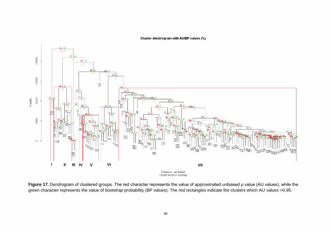
90
Figure 17. Dendrogram of clustered groups. The red character represents the value of approximated unbiased ρ value (AU values), while the
green character represents the value of bootstrap probability (BP values). The red rectangles indicate the clusters which AU values >0.95.
I II III IV V VI VII

91
Figure 18. Clustered fishing grounds off the East Coast Peninsular Malaysia

92
Figure 19. Plotted clustered group of fishing ground by the latitudes and longitudes of each
fishing ground. The diamond points indicate the plot of each fishing ground. The circle points
with standard deviation bars represent the aggregate fishing ground plots.

93
Figure 20. Species composition of clustered groups
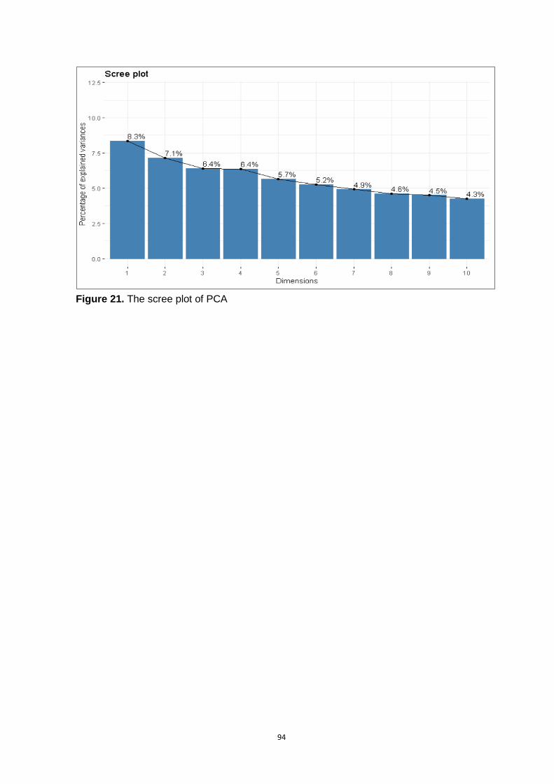
94
Figure 21. The scree plot of PCA

95
Figure 22. The factor map of PCA
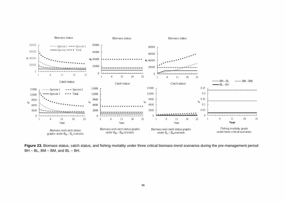
96
Figure 23. Biomass status, catch status, and fishing mortality under three critical biomass-trend scenarios during the pre-management period:
BH – BL, BM – BM, and BL – BH.

97
Figure 24. Kobe-plot for the last management year, after applying the default feedback
harvest control rule (denoted by the abbreviation 1.0-1.0-1.0-0.8), to mixed-species data
(solid colors) and single-species data (outline colors), under three critical biomass-trend
scenarios. Blue, green and orange indicate species 1, 2 and 3, respectively. The shape of
the points denotes the type of biomass-trend scenario, with circles, squares and triangles
used for scenarios BH – BL, BM – BM and BL – BH, respectively. The solid line indicates the
overfishing threshold, while the dashed line defines the overfished line.
0
0.5
1
1.5
2
0 0.5 1 1.5 2
F/F
MS
Y
B/BMSY
(BH - BL) Mix S1 (BH - BL) Mix S2 (BH - BL) Mix S3 (BM - BM) Mix S1 (BM - BM) Mix S2 (BM - BM) Mix S3 (BL - BH) Mix S1 (BL - BH) Mix S2 (BL - BH) Mix S3 (BH - BL) Sin S1 (BH - BL) Sin S2 (BH - BL) Sin S3 (BM - BM) Sin S1 (BM - BM) Sin S2 (BM - BM) Sin S3 (BL - BH) Sin S1 (BL - BH) Sin S2 (BL - BH) Sin S3

98
Figure 25. Biomass and catch status performance of the default feedback harvest control
rule (denoted by the abbreviation 1.0-1.0-1.0-0.8), to mixed-species data (solid colors) and
single-species data (outline colors), under three critical biomass-trend scenarios. Blue,
green, orange and black indicate species 1, 2, 3 and the total species, respectively. The
shape of the points denotes the type of biomass-trend scenario, with circles, squares and
triangles used for scenarios BH – BL, BM – BM and BL – BH, respectively. The solid line
indicates the MSY level, while the dashed line defines the overfished line.
0
0.5
1
1.5
2
0 0.5 1 1.5 2
C/M
SY
B/BMSY
(BH - BL) Mix S1 (BH - BL) Mix S2 (BH - BL) Mix S3 (BH - BL) Mix Total (BM - BM) Mix S1 (BM - BM) Mix S2 (BM - BM) Mix S3 (BM - BM) Mix Total (BL - BH) Mix S1 (BL - BH) Mix S2 (BL - BH) Mix S3 (BL - BH) Mix Total (BH - BL) Sin S1 (BH - BL) Sin S2 (BH - BL) Sin S3 (BH - BL) Sin Total (BM - BM) Sin S1 (BM - BM) Sin S2 (BM - BM) Sin S3 (BM - BM) Sin Total (BL - BH) Sin S1 (BL - BH) Sin S2 (BL - BH) Sin S3 (BL - BH) Sin Total

99
Figure 26. Performance measures of the alternative feedback harvest control rules (HCRs), created by modifying the adjusting
parameter k, with mixed-species data (black points) and single-species data (white points), under three critical biomass-trend scenarios
(BH – BL, BM – BM, and BL – BH, denoted by circles, squares and triangles, respectively). The x-axis is the various k-modified feedback
HCRs, and the y-axis is the performance measures, namely biomass status, coefficient of variation (CV) for the biomass, catch status,
CV for the catch, probability of overfishing and management failure

100
APPENDICES

101
Appendix 1. The fisheries management form
Fisheries management form page 1 of 5

102
Fisheries management form page 2 of 5

103
Fisheries management form page 3 of 5
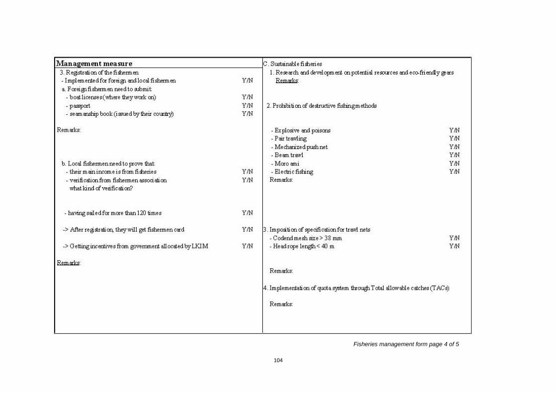
104
Fisheries management form page 4 of 5

105
Fisheries management form page 5 of 5

106
Appendix 2. Fisheries data collection form

107
Appendix 3. Fishery survey form

108
Appendix 4. Biomass and catch trajectories for three species after applying the default feedback harvest control rule (denoted by the abbreviation
1.0-1.0-1.0-0.8) to both mixed-species and single-species data, for BL – BH scenario. Only 20 trajectories are shown in each figure; both σR and
σm were fixed at 0.2. Bold horizontal lines through the biomass and catch trajectories, respectively, indicate the BMSY level and MSY level

109
Appendix 5. Biomass and catch trajectories for three species after applying the default feedback harvest control rule (denoted by the abbreviation
1.0-1.0-1.0-0.8) to both mixed-species and single-species data, for BM – BM scenario. Only 20 trajectories are shown in each figure; both σR and
σm were fixed at 0.2. Bold horizontal lines through the biomass and catch trajectories, respectively, indicate the BMSY level and MSY level.
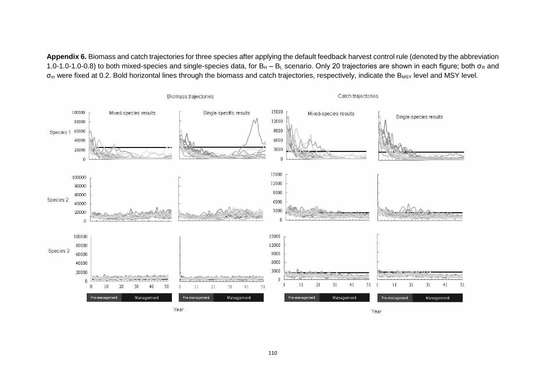
110
Appendix 6. Biomass and catch trajectories for three species after applying the default feedback harvest control rule (denoted by the abbreviation
1.0-1.0-1.0-0.8) to both mixed-species and single-species data, for BH – BL scenario. Only 20 trajectories are shown in each figure; both σR and
σm were fixed at 0.2. Bold horizontal lines through the biomass and catch trajectories, respectively, indicate the BMSY level and MSY level.

111
Appendix 7. Kobe-plot for the last management year, after applying the default feedback
harvest control rule using 𝜎𝑅 = 0.2 and 𝜎𝐼 = 0.4 to mixed-species data (solid colors) and
single-species data (outline colors), under three critical scenarios. Blue, green and orange
indicate species 1, 2 and 3, respectively. The shape of the points denotes the type of
biomass-trend scenario, with circles, squares and triangles used for scenarios BH – BL, BM
– BM and BL – BH, respectively. The solid red line indicates the overfishing threshold, while
the dashed red line defines the overfished line.

112
Appendix 8. Biomass and catch status performance of the default feedback harvest control
rule σ_R = 0.2 and σ_I = 0.4, with mixed-species data (solid colors) and single-species data
(outline colors), under three critical scenarios. Blue, green, orange and black indicate
species 1, 2, 3, and the total species, respectively. The shape of the points denotes the type
of biomass-trend scenario, with circles, squares, and triangles used for scenarios BH – BL,
BM – BM, and BL – BH, respectively. The solid red line indicates the MSY level, while the
dashed red line defines the overfished line.

113
Appendix 9a. Alternative set I of parameter values for the three species in the multispecies fishery under assumption of surplus production
model (Schaefer model) without process error.
Parameter Definition Species 1 Species 2 Species 3
r Intrinsic growth rate 0.5 0.5 0.5
K Carrying capacity 50 000 20 000 10 000
MSY Maximum sustainable yield 2 500 2 500 2 500
BMSY
Biomass produced at the MSY
level 25 000 10 000 5 000
Appendix 9b. Alternative set II of parameter values for the three species in the multispecies fishery under assumption of surplus production
model (Schaefer model) without process error.
Parameter Definition Species 1 Species 2 Species 3
r Intrinsic growth rate 0.2 0.5 1.0
K Carrying capacity 20 000 20 000 20 000
MSY Maximum sustainable yield 2 500 2 500 2 500
BMSY
Biomass produced at the MSY
level 25 000 10 000 5 000

114
Appendix 10. Kobe-plot for the last management year, after applying the default feedback
harvest control rule under alternative set I (Appendix 9a) to mixed-species data (solid color)
and single-species data (outline colors), under three critical scenarios. Blue, green and
orange indicate species 1, 2 and 3, respectively. Shape of the points denotes the type of
biomass-trend scenario, with circles, squares and triangles used for scenarios BH – BL, BM
– BM and BL – BH, respectively. Solid red line indicates the overfishing threshold, while
dashed red line defines the overfished line.
0
0.5
1
1.5
2
0 0.5 1 1.5 2
F/F
MS
Y
B/BMSY
(BH - BL) Mix S1 (BH - BL) Mix S2 (BH - BL) Mix S3
(BM - BM) Mix S1 (BM - BM) Mix S2 (BM - BM) Mix S3
(BL - BH) Mix S1 (BL - BH) Mix S2 (BL - BH) Mix S3
(BH - BL) Sin S1 (BH - BL) Sin S2 (BH - BL) Sin S3
(BM - BM) Sin S1 (BM - BM) Sin S2 (BM - BM) Sin S3
(BL - BH) Sin S1 (BL - BH) Sin S2 (BL - BH) Sin S3

115
Appendix 11. Biomass and catch status performance of the default feedback harvest control rule under alternative set I (Appendix 9a) with mixed-species data (solid colors) and single-species data (outline colors), under three critical scenarios. Blue, green, orange and black indicate species 1, 2, 3, and the total species, respectively. Shape of the points denotes the type of biomass-trend scenario, with circles, squares, and triangles used for scenarios BH – BL, BM – BM, and BL – BH, respectively. Solid red line indicates the MSY level, while dashed red line defines the overfished line.
0
0.5
1
1.5
2
0 0.5 1 1.5 2
C/M
SY
B/BMSY
(BH - BL) Mix S1 (BH - BL) Mix S2 (BH - BL) Mix S3 (BH - BL) Mix Total
(BM - BM) Mix S1 (BM - BM) Mix S2 (BM - BM) Mix S3 (BM - BM) Mix Total
(BL - BH) Mix S1 (BL - BH) Mix S2 (BL - BH) Mix S3 (BL - BH) Mix Total
(BH - BL) Sin S1 (BH - BL) Sin S2 (BH - BL) Sin S3 (BH - BL) Sin Total
(BM - BM) Sin S1 (BM - BM) Sin S2 (BM - BM) Sin S3 (BM - BM) Sin Total
(BL - BH) Sin S1 (BL - BH) Sin S2 (BL - BH) Sin S3 (BL - BH) Sin Total

116
Appendix 12. Kobe-plot for the last management year, after applying the default feedback harvest control rule under alternative set II (Appendix 9b) to mixed-species data (solid colors) and single-species data (outline colors), under three critical scenarios. Blue, green and orange indicate species 1, 2 and 3, respectively. Shape of the points denotes the type of biomass-trend scenario, with circles, squares and triangles used for scenarios BH – BL, BM – BM and BL – BH, respectively. Solid red line indicates the overfishing threshold, while dashed red line defines the overfished line.
0
0.5
1
1.5
2
0 0.5 1 1.5 2
F/F
MS
Y
B/BMSY
(BH - BL) Mix S1 (BH - BL) Mix S2 (BH - BL) Mix S3
(BM - BM) Mix S1 (BM - BM) Mix S2 (BM - BM) Mix S3
(BL - BH) Mix S1 (BL - BH) Mix S2 (BL - BH) Mix S3
(BH - BL) Sin S1 (BH - BL) Sin S2 (BH - BL) Sin S3
(BM - BM) Sin S1 (BM - BM) Sin S2 (BM - BM) Sin S3
(BL - BH) Sin S1 (BL - BH) Sin S2 (BL - BH) Sin S3

117
Appendix 13. Biomass and catch status performance of the default feedback harvest
control rule under alternative set II (Appendix 9b) with mixed-species data (solid colors) and
single-species data (outline colors), under three critical scenarios. Blue, green, orange and
black indicate species 1, 2, 3, and the total species, respectively. Shape of the points
denotes the type of biomass-trend scenario, with circles, squares, and triangles used for
scenarios BH – BL, BM – BM, and BL – BH, respectively. Solid red line indicates the MSY level,
while dashed red line defines the overfished line.
0
0.5
1
1.5
2
0 0.5 1 1.5 2
C/M
SY
B/BMSY
(BH - BL) Mix S1 (BH - BL) Mix S2 (BH - BL) Mix S3 (BH - BL) Mix Total
(BM - BM) Mix S1 (BM - BM) Mix S2 (BM - BM) Mix S3 (BM - BM) Mix Total
(BL - BH) Mix S1 (BL - BH) Mix S2 (BL - BH) Mix S3 (BL - BH) Mix Total
(BH - BL) Sin S1 (BH - BL) Sin S2 (BH - BL) Sin S3 (BH - BL) Sin Total
(BM - BM) Sin S1 (BM - BM) Sin S2 (BM - BM) Sin S3 (BM - BM) Sin Total
(BL - BH) Sin S1 (BL - BH) Sin S2 (BL - BH) Sin S3 (BL - BH) Sin Total

118
Appendix 14. Summary of the performance measures (probability of overfishing [POF], yield status [C/MSY ], biomass status [B/BMSY], management failure [failure], and coefficient of variation [CV]) when applying an alternative harvest control rule (denoted by the abbreviation 0.5-1-1-0.8) to three species (slow-growing [Sp. 1], medium-growing [Sp. 2], and fast-growing [Sp. 3]), with mixed-species data or single-species data, and under three critical biomass-trend scenarios: BH – BL, BM – BM, and BL – BH..
Scenario Performance
measures
Mixed-species results Single-species results
Sp. 1 CV Sp. 2 CV Sp. 3 CV Total CV Sp. 1 CV Sp. 2 CV Sp. 3 CV Total CV
BH – BL
POF 0.81 – 0.06 – 0.00 – – – 0.39 – 0.16 – 0.01 – – –
C/MSY 0.25 0.58 0.66 0.26 0.45 0.29 0.46 – 0.10 0.10 0.50 0.15 0.51 0.19 0.42 –
B/BMSY 0.28 0.56 1.41 0.34 1.66 0.24 0.73 – 0.29 0.26 1.17 0.30 1.62 0.26 0.68 –
Failure 0.01 – 0.00 – 0.01 – 0.02 – 0.60 – 0.19 – 0.01 – 0.68 –
BM – BM
POF 0.36 – 0.00 – 0.00 – – – 0.36 – 0.02 – 0.00 – – –
C/MSY 0.54 0.37 0.52 0.28 0.31 0.31 0.46 – 0.37 0.18 0.53 0.21 0.34 0.20 0.44 –
B/BMSY 0.87 0.46 1.60 0.28 1.76 0.23 1.16 – 0.76 0.40 1.58 0.29 1.73 0.23 1.09 –
Failure 0.00 – 0.00 – 0.01 – 0.01 – 0.22 – 0.01 – 0.01 – 0.23 –
BL – BH
POF 0.00 – 0.00 – 0.00 – – – 0.00 – 0.00 – 0.00 – – –
C/MSY 0.23 0.24 0.12 0.26 0.06 0.28 0.14 – 0.19 0.15 0.12 0.21 0.06 0.20 0.13 –
B/BMSY 1.61 0.35 1.83 0.23 1.87 0.21 1.70 – 1.59 0.34 1.83 0.23 1.89 0.21 1.69 –
Failure 0.00 – 0.00 – 0.00 – 0.00 – 0.00 – 0.00 – 0.00 – 0.00 –

119
Appendix 15. Summary of the performance measures (probability of overfishing [POF], yield status [C/MSY ], biomass status [B/BMSY], management failure [failure], and coefficient of variation [CV]) when applying an alternative harvest control rule (denoted by the abbreviation 1.5-1-1-0.8) to three species (slow-growing [Sp. 1], medium-growing [Sp. 2], and fast-growing [Sp. 3]), with mixed-species data or single-species data, and under three critical biomass-trend scenarios: BH – BL, BM – BM, and BL – BH.
Scenario Performance
measures
Mixed-species results Single-species results
Sp. 1 CV Sp. 2 CV Sp. 3 CV Total CV Sp. 1 CV Sp. 2 CV Sp. 3 CV Total CV
BH – BL
POF 0.83 – 0.04 – 0.00 – – – 0.52 – 0.11 – 0.01 – – –
C/MSY 0.25 0.58 0.68 0.30 0.46 0.29 0.46 – 0.19 0.64 0.61 0.38 0.48 0.35 0.43 –
B/BMSY 0.28 0.53 1.41 0.34 1.66 0.25 0.73 – 0.44 0.68 1.48 0.38 1.64 0.26 0.85 –
Failure 0.00 – 0.00 – 0.00 – 0.00 – 0.05 – 0.01 – 0.01 – 0.07 –
BM – BM
POF 0.36 – 0.00 – 0.00 – – – 0.30 – 0.01 – 0.00 – – –
C/MSY 0.58 0.41 0.53 0.30 0.31 0.30 0.47 – 0.48 0.46 0.52 0.35 0.32 0.33 0.44 –
B/BMSY 0.84 0.44 1.59 0.28 1.77 0.23 1.14 – 0.97 0.51 1.61 0.29 1.76 0.23 1.23 –
Failure 0.00 – 0.00 – 0.00 – 0.00 – 0.00 – 0.00 – 0.00 – 0.00 –
BL – BH
POF 0.00 – 0.00 – 0.00 – – – 0.00 – 0.00 – 0.00 – – –
C/MSY 0.24 0.30 0.13 0.26 0.07 0.27 0.14 – 0.20 0.32 0.11 0.35 0.06 0.33 0.13 –
B/BMSY 1.60 0.35 1.83 0.23 1.90 0.21 1.69 – 1.64 0.36 1.85 0.23 1.86 0.21 1.72 –
Failure 0.00 – 0.00 – 0.01 – 0.01 – 0.00 – 0.00 – 0.01 – 0.01 –

120
Appendix 16. Summary of performance measures (probability of overfishing [POF], yield status [C/MSY ], biomass status [B/BMSY], management
failure [failure], and coefficient of variation [CV]) when applying an alternative harvest control rule (denoted by the abbreviation 2.0-1-1-0.8) to three species (slow-growing [Sp. 1], medium-growing [Sp. 2], and fast-growing [Sp. 3]), with mixed-species data or single-species data, and under three critical biomass-trend scenarios: BH – BL, BM – BM, and BL – BH.
Scenario Performance
measures
Mixed-species results Single-species results
Sp. 1 CV Sp. 2 CV Sp. 3 CV Total CV Sp. 1 CV Sp. 2 CV Sp. 3 CV Total CV
BH – BL
POF 0.83 – 0.04 – 0.00 – – – 0.36 – 0.09 – 0.01 – – –
C/MSY 0.24 0.58 0.68 0.33 0.45 0.30 0.46 – 0.20 0.69 0.61 0.46 0.45 0.44 0.42 –
B/BMSY 0.25 0.52 1.41 0.33 1.70 0.25 0.72 – 0.57 0.66 1.48 0.36 1.70 0.26 0.94 –
Failure 0.00 – 0.00 – 0.00 – 0.00 – 0.01 – 0.01 – 0.01 – 0.03 –
BM – BM
POF 0.35 – 0.00 – 0.00 – – – 0.24 – 0.01 – 0.00 – – –
C/MSY 0.58 0.43 0.53 0.31 0.31 0.31 0.47 – 0.49 0.53 0.48 0.45 0.30 0.43 0.43 –
B/BMSY 0.84 0.43 1.60 0.28 1.77 0.23 1.15 – 1.04 0.47 1.64 0.28 1.78 0.23 1.28 –
Failure 0.00 – 0.00 – 0.00 – 0.00 – 0.00 – 0.00 – 0.01 – 0.01 –
BL – BH
POF 0.00 – 0.00 – 0.00 – – – 0.00 – 0.00 – 0.00 – – –
C/MSY 0.25 0.33 0.13 0.27 0.07 0.28 0.15 – 0.21 0.40 0.11 0.43 0.06 0.41 0.13 –
B/BMSY 1.58 0.35 1.85 0.23 1.87 0.21 1.68 – 1.63 0.35 1.87 0.23 1.87 0.21 1.72 –
Failure 0.00 – 0.00 – 0.01 – 0.01 – 0.00 – 0.00 – 0.01 – 0.01 –

121
Appendix 17. Summary of performance measures (probability of overfishing [POF], yield status [C/MSY ], biomass status [B/BMSY], management failure [failure], and coefficient of variation [CV]) when applying an alternative harvest control rule (denoted by the abbreviation 2.5-1-1-0.8) to three species (slow-growing [Sp. 1], medium-growing [Sp. 2], and fast-growing [Sp. 3]), with mixed-species data or single-species data, and under three critical biomass-trend scenarios: BH – BL, BM – BM, and BL – BH.
Scenario Performance measures
Mixed-species results Single-species results
Sp. 1 CV Sp. 2 CV Sp. 3 CV Total CV Sp. 1 CV Sp. 2 CV Sp. 3 CV Total CV
BH – BL
POF 0.78 – 0.05 – 0.00 – – – 0.30 – 0.09 – 0.01 – – –
C/MSY 0.26 0.61 0.67 0.36 0.44 0.33 0.45 – 0.22 0.75 0.57 0.57 0.42 0.56 0.41 –
B/BMSY 0.30 0.52 1.42 0.33 1.68 0.25 0.75 – 0.68 0.66 1.56 0.36 1.71 0.27 1.03 –
Failure 0.00 – 0.00 – 0.00 – 0.00 – 0.01 – 0.01 – 0.01 – 0.03 –
BM – BM
POF 0.36 – 0.00 – 0.00 – – – 0.22 – 0.01 – 0.00 – – –
C/MSY 0.57 0.46 0.53 0.33 0.31 0.32 0.47 – 0.49 0.62 0.46 0.54 0.29 0.52 0.41 –
B/BMSY 0.82 0.43 1.60 0.27 1.76 0.23 1.13 – 1.12 0.47 1.70 0.28 1.77 0.24 1.35 –
Failure 0.00 – 0.00 – 0.00 – 0.00 – 0.00 – 0.00 – 0.00 – 0.00 –
BL – BH
POF 0.00 – 0.00 – 0.00 – – – 0.00 – 0.00 – 0.00 – – –
C/MSY 0.26 0.36 0.13 0.29 0.07 0.29 0.15 – 0.21 0.50 0.10 0.53 0.06 0.50 0.12 –
B/BMSY 1.59 0.34 1.82 0.23 1.87 0.21 1.68 – 1.65 0.35 1.85 0.23 1.88 0.21 1.73 –
Failure 0.00 – 0.00 – 0.00 – 0.00 – 0.00 – 0.00 – 0.00 – 0.00 –