pushing the limits of natural convection heat transfer ...mbahrami/pdf/theses/thesis m....
TRANSCRIPT

Pushing the Limits of Natural Convection Heat
Transfer from the Heatsinks
by
Mehran Ahmadi
M.Sc., Amirkabir University of Technology, 2010 B.Sc., University of Kerman, 2007
Dissertation/Thesis/ Submitted in Partial Fulfillment of the
Requirements for the Degree of
Doctor of Philosophy
in the
School of Mechatronic Systems Engineering
Faculty of Applied Sciences
Mehran Ahmadi 2014
SIMON FRASER UNIVERSITY
Fall 2014

ii
Approval
Name: Mehran Ahmadi
Degree: Doctor of Philosophy
Title: Pushing the Limits of Natural Convection Heat Transfer from the Heatsinks
Examining Committee: Chair: Kevin Oldknow Lecturer
Majid Bahrami Senior Supervisor Associate Professor
John Jones Supervisor Associate Professor
Jason Wang Supervisor Assistant Professor
Gary Wang Internal Examiner Professor School of Mechatronic System Engineering
Jim Cotton External Examiner Professor Department of Mechanical Engineering McMaster University
Date Defended/Approved:
December 19th, 2014

iii
Partial Copyright Licence

iv
Abstract
This research, which has been done in close collaboration with industrial partners, Alpha
Technologies and Analytic Systems companies, aims to push the current limits of natural
convection heat transfer from vertical heatsinks, with application in passive thermal
management of electronics and power electronics. Advantages such as; being noise-free,
reliable, with no parasitic power demand, and less maintenance requirements, make
passive cooling a preferred thermal management solution for electronics. The focus of this
thesis is to design high performance naturally-cooled heatsinks, to increase the cooling
capacity of available passive thermal management systems. Heatsinks with interrupted
rectangular vertical fins are the target of this study.
Due to the complexities associated with interrupted fins, interrupted rectangular single wall
is chosen as the starting point of the project. Asymptotic solution and blending technique
is used to present a compact correlation for average Nusselt number of such wall, for the
first time. The proposed correlation is verified by the results obtained from numerical
simulations, and experimental data obtained from a custom-designed testbed.
In the next step, natural convection heat transfer from parallel plates has been
investigated. Integral technique is used to solve the governing equations, and closed-form
correlations for velocity, temperature, and local Nusselt number are developed for the first
time. The results are successfully verified with the result of an independent numerical
simulation and experimental data obtained from the tests conducted on heatsink sample.
In the last step, to model heat transfer from interrupted finned heatsinks, and to obtain
compact correlations for velocity and temperature inside the domain, an analytical
approach is used. Numerical simulations are performed to provide the information required
by our analytical approach. An extensive experimental study is also conducted to verify
the results from analytical solution and numerical simulation. Results show that the new-
designed heatsinks are capable of dissipating heat five times more than currently available
naturally-cooled heatsinks, with a weight up to 30% less. The new heatsinks can increase
the capacity of passive-cooled systems significantly.
Keywords: Natural convection; Heatsink; Interrupted fins; Analytical solution; Experimental study; Numerical simulation

v
Dedication
To my beloved parents, my dear brothers, and my best
friend Maryam

vi
Acknowledgements
I would like to thank my senior supervisor, Dr. Majid Bahrami, for his kind support,
guidance, and insightful discussions throughout this research. It was a privilege for me to
work with him and learn from his experience.
I am also indebted to Dr. John Jones and Dr. Jason Wang for the useful discussions and
comments, which helped me to define the project and to pursue its goals. I would also like
to thank Dr. Gary Wang and Dr. Jim Cotton for their time reading this thesis and helping
to refine it.
I would like to thank my colleagues and lab mates at Laboratory for Alternative Energy
Conversion at Simon Fraser University. Their helps, comments, and assistance played an
important role in the development of this thesis. In particular, I want to thank Mohammad
Fakoor Pakdaman, Ali Gholami, Marius Haiducu, and Peyman Taheri.
I have received financial support from Natural Sciences and Engineering Research
Council (NSERC) of Canada, Mathematics of Information Technology and Complex
Systems (MITACS), Alpha Technologies, Analytic Systems, and Simon Fraser University,
for which I am grateful. I would also like to appreciate our industrial collaborators,
specifically Mr. Kevin Lau, Mr. Steve Pratt, and Mr. Rajiv Witharana for their time, help
and kind cooperation.
I have to thank my family that have endlessly encouraged and supported me through all
stages of my life. Without their presence and support no achievement was possible in my
life. I would also like to thank my dear friends; Hossein Dehghani, Soheil Sadeqi, Arash
Tavassoli, Kambiz Haji Hajikolahi, and Fattane Nadimi for their kind support and great
memories. Finally special thanks to my best friend, Maryam Yazdanpour for her kind
companionship, understanding, and devotion.

vii
Table of Contents
Approval .......................................................................................................................... ii Partial Copyright Licence ............................................................................................... iii Abstract .......................................................................................................................... iv Dedication ....................................................................................................................... v Acknowledgements ........................................................................................................ vi Table of Contents .......................................................................................................... vii List of Tables .................................................................................................................. ix List of Figures.................................................................................................................. x List of Acronyms ............................................................................................................ xii Symbols ........................................................................................................................ xiii Executive Summary ......................................................................................................xvi Motivation ......................................................................................................................xvi Objectives .................................................................................................................... xvii Methodology ................................................................................................................ xvii Contributions ............................................................................................................... xviii
Chapter 1. Introduction ............................................................................................. 1 1.1. Research Importance ............................................................................................. 1 1.2. Research Motivation ............................................................................................... 3 1.3. Research Scope ..................................................................................................... 4 1.4. Thesis Structure ..................................................................................................... 5 1.5. Literature Review .................................................................................................... 6 1.6. Research Objectives ............................................................................................ 11
Chapter 2. Natural Convection from Interrupted Vertical Walls ........................... 12 2.1. Numerical Analysis ............................................................................................... 13
2.1.1. Governing Equations ............................................................................... 13 2.1.2. Mesh Independency ................................................................................ 15
2.2. Experimental Study .............................................................................................. 18 2.2.1. Testbed ................................................................................................... 18 2.2.2. Test Procedure ........................................................................................ 20 2.2.3. Uncertainty Analysis ................................................................................ 21
2.3. Results and Discussion ........................................................................................ 23 2.4. Conclusion ............................................................................................................ 29
Chapter 3. Natural Convection from Vertical Parallel Plates ................................ 30 3.1. Problem Statement ............................................................................................... 30
3.1.1. Governing Equations and Boundary Conditions ...................................... 31 3.2. Present Solution ................................................................................................... 33
3.2.1. Entrance Velocity ..................................................................................... 33 3.2.2. Integral Technique ................................................................................... 34
3.3. Numerical Simulation ............................................................................................ 37 3.4. Experimental Study .............................................................................................. 39

viii
3.4.1. Testbed ................................................................................................... 40 3.4.2. Uncertainty Analysis ................................................................................ 42
3.5. Results and Discussion ........................................................................................ 42 3.6. Conclusion ............................................................................................................ 45
Chapter 4. Natural Convection from Interrupted Fins ........................................... 46 4.1. Problem Statement ............................................................................................... 46 4.2. Solution Methodology ........................................................................................... 47
4.2.1. Channel Flow .......................................................................................... 48 4.2.2. Gap Flow ................................................................................................. 49
Governing equations and boundary conditions ..................................................... 50 Integral technique................................................................................................... 52
4.3. Numerical Simulation ............................................................................................ 54 4.4. Experimental Study .............................................................................................. 57
4.4.1. Testbed ................................................................................................... 58 4.4.2. Test Procedure ........................................................................................ 59 4.4.3. Uncertainty Analysis ................................................................................ 61 4.4.4. Test Results ............................................................................................ 61 4.4.5. Validity of Uniform Wall Temperature Assumption ................................... 63
4.5. Results and Discussion ........................................................................................ 64 4.5.1. Total Heat Transfer Calculation ............................................................... 64 4.5.2. Parametric Study ..................................................................................... 66
Effect of Fin Spacing .............................................................................................. 66 Effect of Gap Length .............................................................................................. 66 Effect of Fin Length ................................................................................................ 67
4.5.3. Heatsink Design Procedure ..................................................................... 70 4.6. Conclusion ............................................................................................................ 71
Chapter 5. Summary and Future Work ................................................................... 72 5.1. Summary of Thesis ............................................................................................... 72 5.2. Future Work .......................................................................................................... 73
References ................................................................................................................ 75 Appendix A. Integral Method for Natural Convection ............................................ 82
Conservation of mass ........................................................................................... 83 Conservation of momentum .................................................................................. 84 Conservation of energy ......................................................................................... 85
Appendix B. Calculation of Radiation Heat Transfer from Test Samples .............. 86 Emissivity measurement ....................................................................................... 87

ix
List of Tables
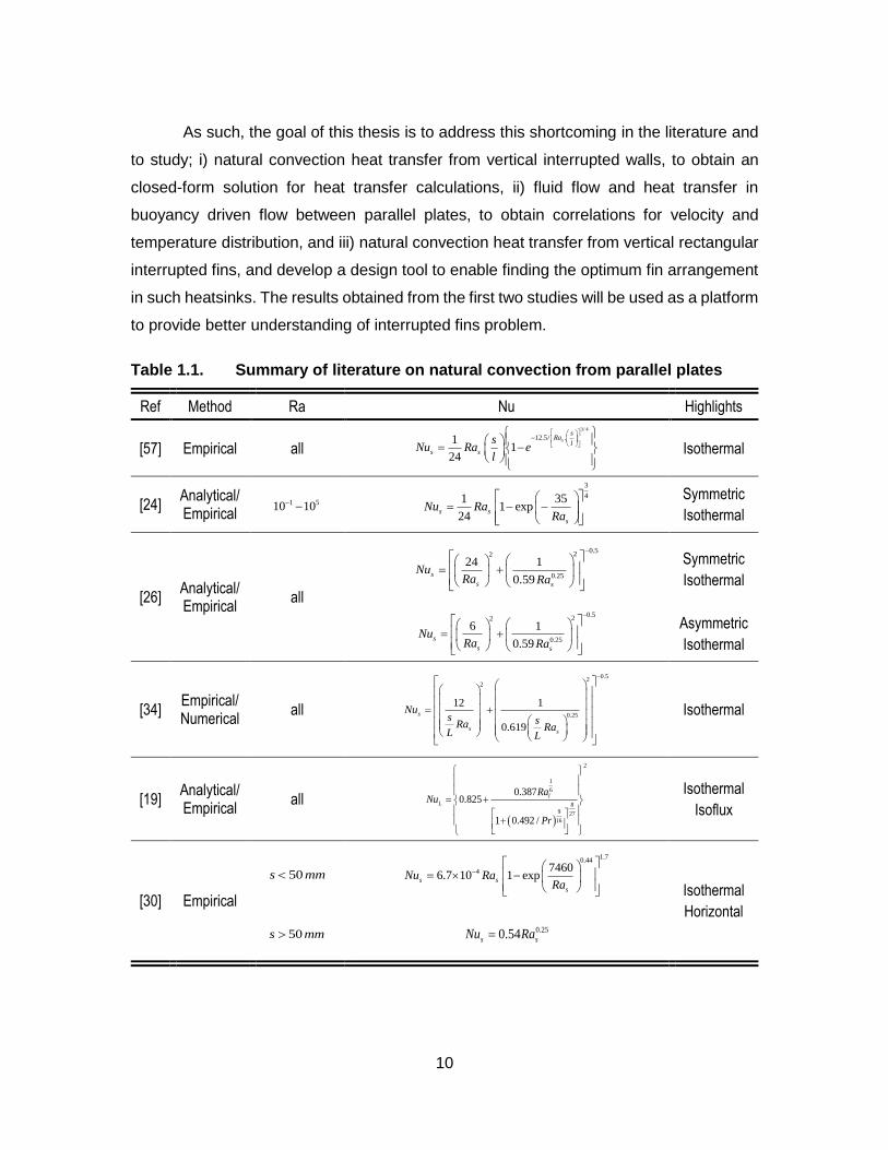
Table 1.1. Summary of literature on natural convection from parallel plates ............ 10
Table 2.1. Parameters used in the benchmark case for numerical simulations ....... 16
Table 2.2. Dimensions of the interrupted wall samples used in experimental study ...................................................................................................... 19
Table 2.3. Range of important parameters in the experimental study ...................... 21
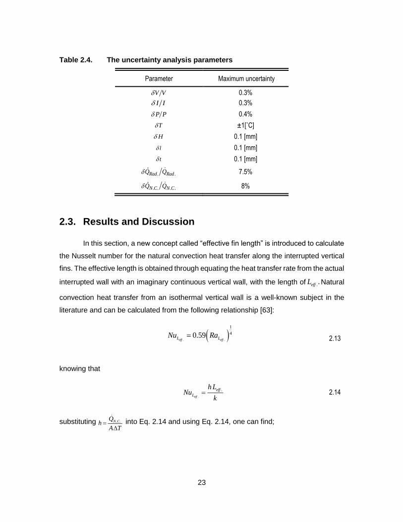
Table 2.4. The uncertainty analysis parameters ...................................................... 23
Table 3.1. Integral form of conservation equations for the integral control volume ................................................................................................... 33
Table 3.2. Dimensionless parameters ..................................................................... 36
Table 3.3. Parameters used for the numerical simulation benchmark ..................... 38
Table 3.4. Dimensions of the finned plate samples ................................................. 40
Table 4.1. Parameters used for numerical simulation benchmark case ................... 55
Table 4.2. Dimensions of the interrupted fin samples used in the experiments ....... 59
Table 4.3. Range of some important parameters in test procedure ......................... 60

x
List of Figures
Figure 1.1. Industrial collaborators products, a) Analytic Systems naturally-cooled power enclosure, b) Alpha technologies outside plant power cabinet. .......................................................................................... 3
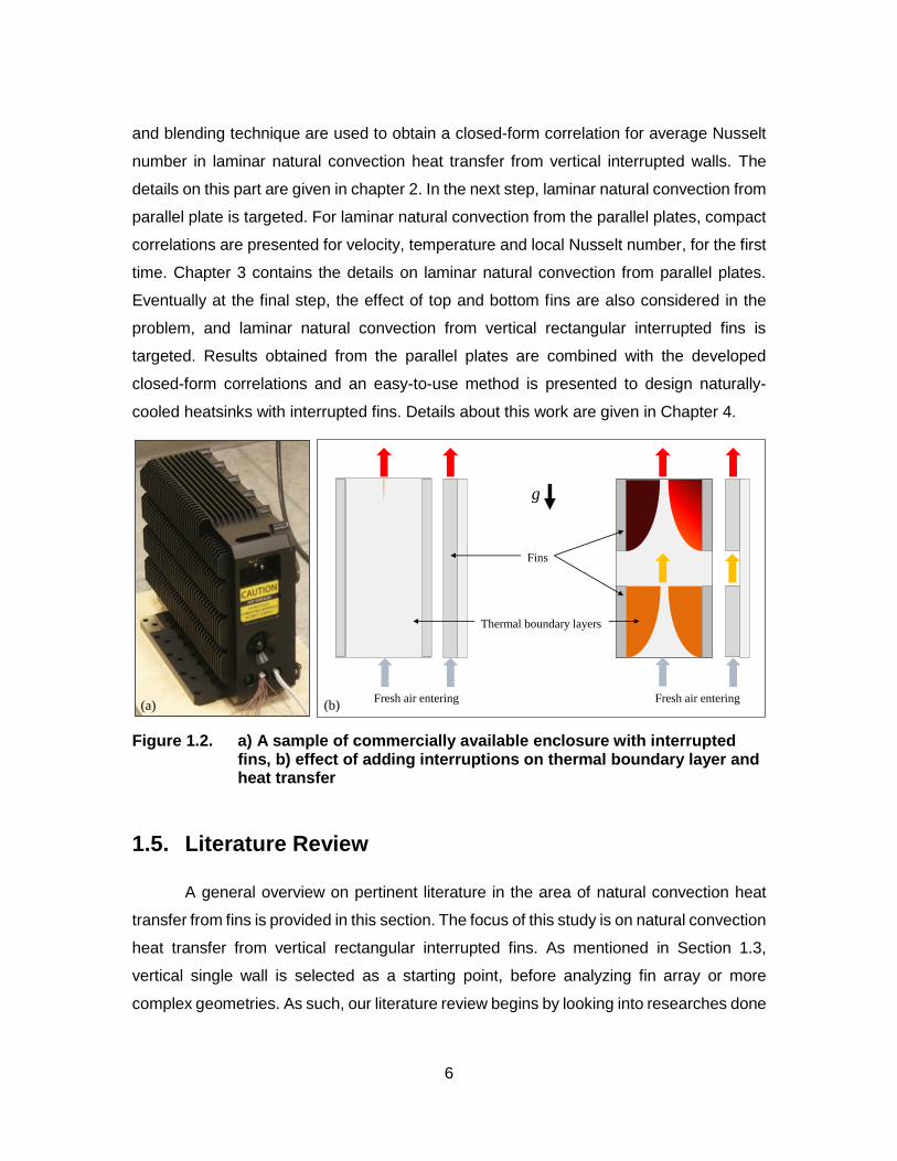
Figure 1.2. a) A sample of commercially available enclosure with interrupted fins, b) effect of adding interruptions on thermal boundary layer and heat transfer ...................................................................................... 6
Figure 2.1. Effect of interruptions on boundary layer growth in natural heat transfer from a vertical wall .................................................................... 13
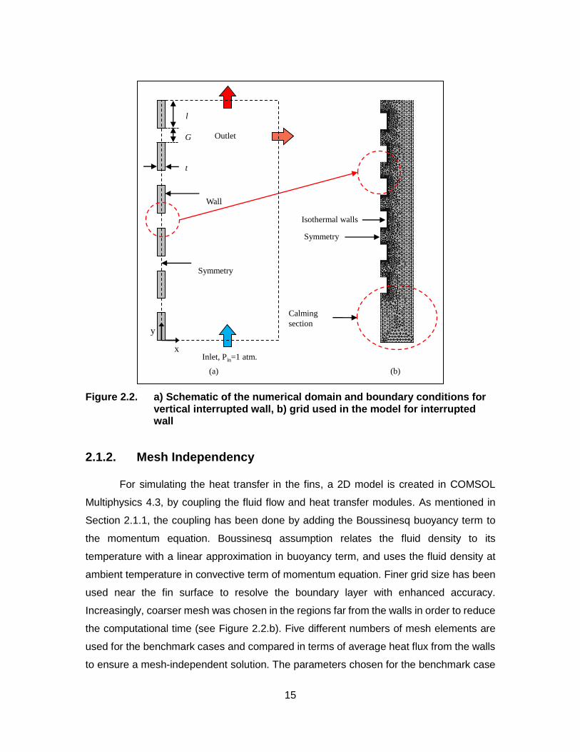
Figure 2.2. a) Schematic of the numerical domain and boundary conditions for vertical interrupted wall, b) grid used in the model for interrupted wall......................................................................................................... 15
Figure 2.3. Grid independency study; walls average heat flux versus number of elements for the benchmark case (see Table 2.1) .............................. 16
Figure 2.4. a) velocity domain, and b) temperature domain for the benchmark case; the diffusion of velocity and temperature in the gap causes the air to reach the top wall with higher velocity and lower temperature ............................................................................................ 17
Figure 2.5. a) schematic and photo of the testbed; b) backside of the samples; positioning of the thermocouples and heater ........................... 19
Figure 2.6. Heat transfer versus /G l for different /l t values. The figure
also shows the comparison between the numerical data (symbols) and introduced asymptotes (Lines)......................................................... 26
Figure 2.7. Effective length versus /G l for different /l t values. The
figure also shows the comparison between the numerical data (symbols) and the proposed correlation (lines) for the effective length. .................................................................................................... 27
Figure 2.8. Nusselt number versus /G l for different /l t values. The
figure also shows the comparison between the numerical data (hollow symbols), experimental data (solid blue symbols), and the proposed compact relationship (lines) .................................................... 28
Figure 3.1. a) a naturally-cooled enclosure of a power converter; b) schematic of the heatsink, and c) solution domain, selected as the control volume ................................................................................................... 31
Figure 3.2. a) schematic of the numerical domain and boundary conditions, b) the grid used in the model, c) velocity domain, and d) temperature domain for the benchmark case ............................................................. 38
Figure 3.3. Grid independency study; walls average heat flux versus number of elements for the benchmark case (see Table 3.3) .............................. 39

xi
Figure 3.4. a) schematic of the test-bed; b) samples dimensions, heater and thermocouples positioning; c) testbed casing and insulation; and d) a photo of the testbed ........................................................................ 41
Figure 3.5. Comparison between the analytical solution (lines), a) velocity b) temperature distribution and numerical results (symbols) at various cross sections along the channel ............................................... 43
Figure 3.6. Comparison between the present average Nusselt number, existing semi-empirical relations in the literature [24] and [26], and our experimental data ............................................................................ 45
Figure 4.1. A schematic of heatsink with interrupted fins, geometrical parameters used to address fin parameters, and the regions related to channel flow and gap flow ...................................................... 47
Figure 4.2. Schematic of the control volume selected for the channel flow ............... 49
Figure 4.3. Schematic of the control volume selected for the gap flow ..................... 50
Figure 4.4. Numerical simulation-benchmark case; a) the domain and boundary condition, b) a sample of mesh, c) velocity distribution, and d) temperature distribution ............................................................... 55
Figure 4.5. Mesh independency study for the benchmark case ................................ 56
Figure 4.6. Comparison between the result from integral technique with40 and 95, and numerical simulations at the benchmark
case , a) velocity domain, b) temperature domain .................................. 57
Figure 4.7. Experimental setup, a) the position of thermocouples and the heater, b) photos of sample under test, c) schematic of the test bed and insulations ................................................................................ 58
Figure 4.8. Comparison between the experimental data and analytical solution, a) fin spacing, b) fin length, c) gap length ................................. 62
Figure 4.9. IR image from a) front view, b) side view of the heatsink sample under test ............................................................................................... 64
Figure 4.10. Effect of fin spacing on heat transfer from the heatsink .......................... 66
Figure 4.11. Effect of gap length on heat transfer from the heatsink, a) total heat transfer, b) dimensionless heat transfer with respect to continuous fins ....................................................................................... 68
Figure 4.12. Effect of fin length on heat transfer from the heatsink, a) total heat transfer, b) dimensionless heat transfer with respect to continuous fins 69
Figure 5.1. Proposed geometries for the future work, a) inclined interrupted fins, b) variable fin parameters along the flow ........................................ 74

xii
List of Acronyms
DAQ Data Acquisition System
GA Genetic Algorithm
IR Infrared
LED Light-Emitting Diode
PMMA Poly Methyl Methacrylate
TCR Thermal Contact Resistance
TIM Thermal Interface Material

xiii
Symbols
General Symbols
A Surface area, m2
c Constant of blending technique in effective length
pc Specific heat, J/kg.K
E Energy, W
F Force, N
g Gravitational acceleration, m/s2
G Gap length, m
Gr Grashof number, gβΔTs3/ν2
h Heat transfer coefficient, W/m2K
H Fin height, m
k Thermal conductivity, W/m.K
l Fin length, m
L Baseplate length, m
m Number of fin rows
m Mass flow rate, kg/s
M Momentum, kg.m/s
n Number of fin columns
Nu Nusselt number, hs/k
p Pressure, Pa
P Heater power, W
Pr Prandtl number, ν/α
q Heat flux, W/m2
Q Total heat transfer, W
Ra Rayleigh Number, gβΔTs3/να
s Fin spacing, m
t Thickness, m
T Temperature, K
u Velocity in x-direction, m/s
U Dimensionless velocity in x-direction, us/α
xiv
v Velocity in y-direction, m/s
W Baseplate width, m
x Direction parallel to fins, m
X Dimensionless x, x/l
y Direction normal to fins, m
Y Dimensionless y, y/s
z Direction normal to x and y in Cartesian coordinate
Greek Symbols
Thermal diffusivity, m2/s
Coefficient of volume expansion, K-1
Coefficient appears in channel velocity
Coefficient appears in channel temperature
Difference
Channel slenderness, l/s
Coefficient appears in gap velocity
Coefficient appears in gap velocity
Parameter appears in channel temperature, 1/m
Coefficient appears in channel temperature
Coefficient appears in gap temperature
Gap to fin length ratio in interrupted walls, G/l
Parameter appears in channel velocity, 1/m
Dynamic viscosity, kg/m.s
Kinematic viscosity, m2/s
Dimensionless temperature, (Tw-T)/(Tw-T∞)
Constant appears in gap temperature
Density, kg/m3
Parameter appears in gap temperature, 1/m
Parameter appears in gap velocity, 1/m
Shear stress, N/m2
R Uncertainty
Gap width, m
Constant appears in channel velocity

xv
Fin length to thickness ratio in interrupted walls, l/t
Subscripts
Ambient properties
b Baseplate
bottom Fin’s bottom in interrupted walls
C Channel
. .C V Control volume
ends Fin’s top/bottom in interrupted walls
.eff Effective
. .F D Fully developed
G Gap
in Inlet of channel/gap
. .N C Natural convection
out Outlet of channel/gap
.Rad Radiation
sides Fin’s sides in interrupted walls
top Fin’s top in interrupted walls
total Total heat transfer
w Wall properties

xvi
Executive Summary
Motivation
Thermal management of electronics/power electronics has wide applications in
different industries such as; telecommunication, automotive, and renewable energy
systems. About 55% of failures in electronics during operation have thermal root. The rate
of failure due to overheating nearly doubles with every 10°C increase above the operating
temperature. The importance of efficient thermal management systems is reflected in their
worldwide market. Thermal management technology market was valued at $10.1 billion in
2013 and reached $10.6 billion in 2014. Total market value is expected to reach $14.7
billion by 2019. Thermal management hardware, such as fans and heatsinks, accounts
for about 84% of the total market.
Passive cooling is a widely preferred cooling method for electronic and power
electronic devices. High reliability, no noise and no parasitic power make passive cooling
methods such as natural convection, attractive for sustainable and “green” systems.
Telecommunication devices are an example of electronic systems that require efficient
thermal management. More than 1% of global total energy consumption (3% of US energy
consumption) in 2012 was used by telecommunication devices. This is equal to energy
consumed by 15 million US homes. About 28% of this energy is required for thermal
management of such systems. Studies show that applying passive cooling techniques can
reduce the energy required for thermal management from 28% of total energy
consumption to 15% in general and 0% in some cases.
In any typical thermal management system, passive or active, there is always a
temperature difference between the heat source and cooling medium, called thermal
budget, which is the driving force of heat transfer. This thermal budget is spent in the
thermal resistances along the heat path. The thermal resistances, in most cases include:
i) thermal contact resistance at the solid-solid interface due to surface asperities, ii)
spreading resistance, due to changes in geometry and bottle necks, iii) bulk resistance,
due to material thermo-physical properties, and iv) film resistance existing at the solid-fluid
interface due to boundary layer effects. Except for the film resistance, the rest of the
above-mentioned thermal resistances act similarly between active and passive cooling
xvii
systems. The effect of film resistance appears in the heatsink, and consequently design
of high performance naturally-cooled heatsinks becomes very important in design of next
generation passive thermal management system. This thesis aims to address the need,
for this design by pushing the limits of natural convection heat transfer from heatsinks.
Objectives
The research objectives are:
• To increase the current heat dissipation limit of naturally-cooled heatsinks, by using interrupted fins instead of conventional fins
• To establish a deep understanding of air flow and heat transfer in naturally-cooled heatsinks
• To develop a design tool for high performance naturally-cooled heatsinks with interrupted fins
• To find the optimum fin arrangement on naturally-cooled heatsinks to maximize the heat transfer
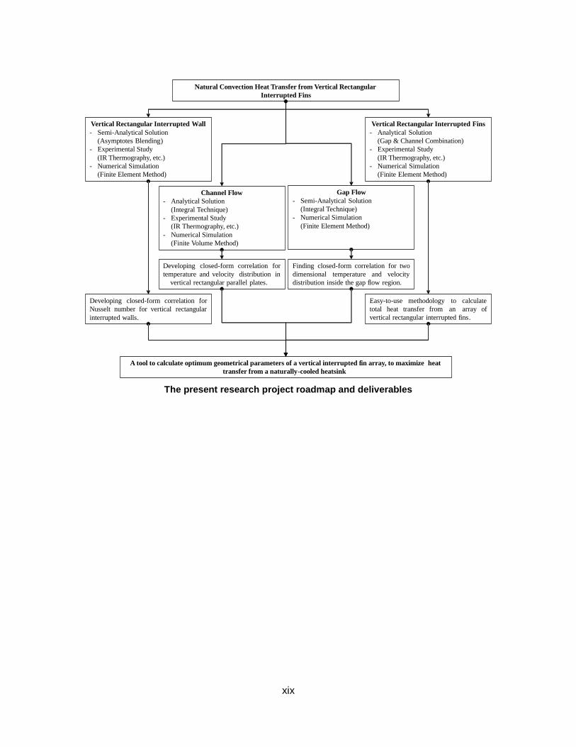
Methodology
This research is focused on film resistance due to thermal boundary layer, which
occurs at the solid-fluid interface in the heatsinks. The target of this research is naturally-
cooled heatsinks with vertical rectangular interrupted fins, for which no in-depth study was
found in the available literature. The research project is divided into three main sub-
projects; i) interrupted single wall, ii) natural convection from parallel plates, and iii) natural
convection from interrupted fins. Figure 1 shows more details on sub-projects and the
roadmap for the main project.
Analytical modeling is used to solve the governing equations for velocity and
temperature domain for each sub-project. Integral technique, asymptotic solution, and
blending technique are the main mathematical methods used in this research. Numerical
simulations are also conducted for each sub-project, to get better understanding of the
physics of the flow, and to verify some analytical results. Commercial software packages,
COMSOL Multiphysics and ANSYS FLUENT, are used for numerical modeling. At the
end, all the obtained correlations are validated by experimental data, obtained from the

xviii
custom-designed testbeds, made in the lab. More than 30 heat sinks samples, related to
all three sub-projects, are machined out of aluminum and tested.
Results show that our designed heatsinks are capable of dissipating heat up to 12
times more than available naturally-cooled heatsinks, with up to 30% lower weight. The
average heat transfer improvement in the designed heatsinks compared to commercially
available heatsinks is 500%.
Contributions
The list of contributions resulted from the present study is listed below;
• Developing a closed-form correlation for average Nusselt number for interrupted single walls, published in ASME Journal of Heat Transfer
• Developing closed-form solutions for local Nusselt number, velocity, and temperature distribution in laminar natural convection heat transfer between parallel plates, published in Journal of Thermophysics and Heat Transfer
• Developing compact correlation for velocity and temperature in two dimensional momentum and energy diffusion in a one directional laminar flow
• Design of interrupted fins naturally-cooled heatsinks with average heat dissipation of 5 time higher than similar commercially available heatsinks
• Developing an easy to use tool to design high performance naturally-cooled heatsinks with interrupted fins, published in International Journal of Thermal Sciences
• Design and prototyping of a fully passive thermal management system for outside plant telecom enclosures, presented in IEEE INTELEC 2014 Conference
xix
The present research project roadmap and deliverables
Natural Convection Heat Transfer from Vertical Rectangular
Interrupted Fins
Vertical Rectangular Interrupted Wall
- Semi-Analytical Solution
(Asymptotes Blending)
- Experimental Study
(IR Thermography, etc.)
- Numerical Simulation
(Finite Element Method)
Channel Flow
- Analytical Solution
(Integral Technique)
- Experimental Study
(IR Thermography, etc.)
- Numerical Simulation
(Finite Volume Method)
Gap Flow
- Semi-Analytical Solution
(Integral Technique)
- Numerical Simulation
(Finite Element Method)
Vertical Rectangular Interrupted Fins
- Analytical Solution
(Gap & Channel Combination)
- Experimental Study
(IR Thermography, etc.)
- Numerical Simulation
(Finite Element Method)
Developing closed-form correlation for
Nusselt number for vertical rectangular
interrupted walls.
Developing closed-form correlation for
temperature and velocity distribution in
vertical rectangular parallel plates.
Finding closed-form correlation for two
dimensional temperature and velocity
distribution inside the gap flow region.
Easy-to-use methodology to calculate
total heat transfer from an array of
vertical rectangular interrupted fins.
A tool to calculate optimum geometrical parameters of a vertical interrupted fin array, to maximize heat
transfer from a naturally-cooled heatsink
1
Chapter 1. Introduction
1.1. Research Importance
Thermal management of electronics and power electronics has vast applications
in several industries such as; telecom industry (datacenters and outdoor enclosures),
automotive industry (conventional vehicles, hybrid vehicles, electric vehicles, and fuel cell
vehicles), renewable energy systems (solar panels and wind turbine power electronics),
aerospace industry, and light-emitting diode (LED) industry. Efficient thermal management
of electronics is essential for optimum performance and durability. About 55% of failures
in electronics during operation have a thermal root [1]. The rate of failures due to
overheating nearly doubles with every 10°C increase above the operating temperature [2].
Considering the increasing functionality and performance of electronic devices and the
ever increasing desire for miniaturization in the industry, thermal management has
become the limiting factor in the development of such devices, specifically in case of
telecom power-electronics [3], and LEDs [4,5], and reliable low-cost cooling methods are
more and more required. The importance of electronics thermal management is also
reflected in its worldwide market. Thermal management technology market was valued at
$10.1 billion in 2013 and reached $10.6 billion in 2014 [6]. Total market value is expected
to reach $14.7 billion by 2019. Thermal management hardware, e.g. fans and heatsinks,
account for about 84% of the total market. Other cooling product segments, e.g. software,
thermal interface materials (TIM), and substrates, each account for between 4% to 6% of
the market [6].
Passive cooling is a widely preferred cooling method for electronic and power
electronic devices since it is economical, quiet, and reliable. Moreover, natural convection
and other passive cooling solutions require no parasitic power which make them more
attractive for sustainable and “green” systems. Telecommunication devices are an
2
example of power electronic systems that require efficient thermal management. More
than 1% of global total energy consumption ( 3% of U.S. energy consumption) in 2013 is
used by telecommunication devices [7], which is equal to annual energy consumed by 15
million US homes, with equivalent CO2 emission of 29 million cars [8,9]. This value is
predicted to increase by 50% by 2017 [10]. About 28% of this energy is required for
cooling and thermal management of such systems [11]. Integrating passive cooling
techniques with conventional cooling strategies, can reduce this value to 15% [12] in
general. Energy demand for cooling can be decreased to 0% [13] if fully-passive thermal
management systems are designed and used. As such, passive cooling systems have
attracted an immense attention especially in the renewable energy conversion systems
and applications in which energy efficiency is of major importance, or applications where
using a fan is not essential or possible, e.g. hostile environment, contaminated air,
vibration-sensitive systems, noise-limiting regulations, and high levels of humidity.
In any typical thermal management system, passive or active, there is always a
temperature difference between the heat source and cooling medium, called thermal
budget, which is the driving force of heat transfer. This thermal budget is spent in the
thermal resistances along the heat path. The thermal resistances, in most cases include;
i) thermal contact resistance at the solid-solid interface due to surface asperities, ii)
spreading resistance, due to bottle necks and changes in geometry, iii) bulk resistance,
due to material thermo-physical properties, and iv) film resistance at the solid-fluid
interface due to boundary layer effects. Except for the film resistance, the above-
mentioned thermal resistances are similar between active and passive cooling systems.
The effect of film resistance appears in the heatsink, and consequently design of high
performance naturally-cooled heatsinks becomes crucial in design of reliable passive
thermal management system. Heatsinks are common components of almost all thermal
management systems. They are used to dissipate the generated heat in electronic
components to the ambient. Heat generating components could be; i) high-power
semiconductor devices, such as diodes, Thyristors, IGBTs and MOSFETs, ii) integrated
circuits, such as audio amplifiers, microcontrollers and microprocessors, or iii) other
electronics such as LEDs or CPUs. To increase the effectiveness and performance of
heatsinks, they are usually manufactured with extended surfaces, also known as fins. Fins
are used to increase the rate of heat transfer by increasing the surface area. Different fin

3
geometries are being used in the industry and studied in the literature including;
rectangular, circular, conical, pin fins, etc. Orientation of fins, i.e. vertical, horizontal, or
inclined, also plays an important role in heatsinks performance.
1.2. Research Motivation
This work has been impelled by a collaborative research project with two local
companies; Analytic Systems, a manufacturer of electronic power conversion systems
located in Delta, BC, and Alpha Technologies Ltd, a telecom and power solution company
located in Burnaby, BC. Both companies were interested in passive cooling solutions for
their power electronic systems. Some of the Analytic Systems naturally-cooled enclosures
experienced excessive heating causing reliability and performance issues for their clients.
Therefore, a research venture was initiated with Analytic Systems with the goal of
modifying the naturally-cooled power enclosure to resolve the thermal management
problem. Alpha Technologies on the other side, was seeking a fully passive cooling
solution for their outside plant power enclosures, used in telecom industry. Their goal was
to convert their current fan-assisted heat exchanger-equipped thermal management
system of their power enclosures to a fully passive cooling solution. Figure 1.1 shows the
sample products from Analytic Systems and Alpha technologies. As such, parallel to the
Analytic Systems project, a new research collaboration started with Alpha Technologies,
both sharing the concept of passive thermal management systems of power electronics.
Figure 1.1. Industrial collaborators products, a) Analytic Systems naturally-cooled power enclosure, b) Alpha technologies outside plant power cabinet.
(a) (b)

4
1.3. Research Scope
As mentioned in Section 1.2, the goal of the industrial projects at system level is
to design a passive thermal management system for power enclosures. Although the
projects are defined for different applications, they share similar architecture for the
cooling system. The heat generated at the electrical components should pass through a
thermal interface material (TIM) that provides the electrical insulation and minimizes the
thermal contact resistance (TCR), spread inside a heat spreader that connects the small
area of the heat generating component to a larger part in which heat can transfer more
easily, pass through a medium to reach the heatsink, and eventually dissipate to the
ambient via convection and radiation. Thermal resistances existing in the heat path, can
affect the quality of the heat transfer significantly, by spending the available thermal
budget in an ineffective way. Thermal budget is the available temperature difference
between the heat source and cooling medium. Thermal resistances, in most cases,
include: i) thermal contact resistance at the solid-solid interface due to surface asperities,
ii) spreading resistance, occurring in the geometrical bottle necks, iii) bulk resistance, due
to material thermo-physical properties, and iv) film resistance existing at the solid-fluid
interface due to boundary layer effects. In an efficient thermal management system, all
the above-mentioned resistances should be minimized. Therefore the main projects are
divided to sub-projects, each focusing on one thermal resistance. The target is to get better
understanding of each resistance by doing fundamental research including; mathematical
modeling, experimental study, and numerical simulation. Each part is assigned to a
graduate student, and at the end the results gathered from sub-projects at the component
level, are integrated at system level to design a fully passive thermal management system
for power electronic enclosures. The sub-project related to thermal spreading resistance
is successfully finished by another researcher at Laboratory for Alternative Energy
Conversion (LAEC), and more details can be found in [14]. The other sub-project with goal
of minimizing the thermal contact resistance (TCR), is targeting the thermal interface
materials (TIMs), and is currently an ongoing research at LAEC, conducted by another
researcher. The focus of the research in this thesis, is on the film resistance at the solid-
fluid interface, which is related to the design of high performance naturally-cooled
heatsinks. At the system level, a heatpipe-integrated fully-passive thermal management

5
system is designed, built, and successfully tested, by the author. The results of the system
level design, are presented in INTELEC 2014 conference [15].
1.4. Thesis Structure
The main challenge in heatsink design is to find the best geometry, orientation,
and arrangement for the fins, to maximize the heat transfer from a given surface area. In
the quest to find the best fin arrangement, some of the pioneer industries in the field are
noticed to be using a specific fin arrangement, namely “interrupted fins” or “discrete fins”
(Figure 1.2.a). However, as shown in Section 1.5, our literature review shows that no in-
depth study has been performed to investigate the external laminar natural convection
heat transfer from interrupted fins, and the parameters for currently used interrupted fins
are solely selected by a trial and error process. It is expected that proper selection of
geometrical parameters leads to a higher thermal performance, which is based on the fact
that interrupted fins disrupt the thermal boundary layer growth, and maintain a thermally
developing flow regime along the fins which leads to higher heat flux dissipated from the
heatsink (Figure 1.2.b). Fin interruption also results in a considerable weight reduction,
however on the other hand, adding interruption to fins leads to losing surface area, which
decreases the total heat transfer. These two competing trends clearly indicate that an
“optimum” fin arrangement exists that will provide the maximum heat transfer rate from
naturally-cooled heatsinks. The main goal of this thesis is to find the optimum fin
arrangement for naturally-cooled heatsinks with vertical rectangular interrupted fins.
The governing equations of natural convection heat transfer are rather complex
partial differential equations to be solved analytically. The reason for this complexity is that
the driving force of fluid flow in natural convection is buoyancy force, while this body force
itself is result of fluid density change due to temperature variation. Consequently,
momentum and energy equations are coupled in the conservation equations, and
temperature term appears in the momentum equation. When natural convection occurs in
open ended channels, buoyancy force effect causes a fluid flow between the channel walls
that makes the evaluation of inlet boundary conditions rather difficult. At the first step, in
order to get rid of this complication, the neighboring fins are eliminated from the geometry
to create an interrupted vertical wall. After simplifying the problem, asymptotic solution
6
and blending technique are used to obtain a closed-form correlation for average Nusselt
number in laminar natural convection heat transfer from vertical interrupted walls. The
details on this part are given in chapter 2. In the next step, laminar natural convection from
parallel plate is targeted. For laminar natural convection from the parallel plates, compact
correlations are presented for velocity, temperature and local Nusselt number, for the first
time. Chapter 3 contains the details on laminar natural convection from parallel plates.
Eventually at the final step, the effect of top and bottom fins are also considered in the
problem, and laminar natural convection from vertical rectangular interrupted fins is
targeted. Results obtained from the parallel plates are combined with the developed
closed-form correlations and an easy-to-use method is presented to design naturally-
cooled heatsinks with interrupted fins. Details about this work are given in Chapter 4.
Figure 1.2. a) A sample of commercially available enclosure with interrupted fins, b) effect of adding interruptions on thermal boundary layer and heat transfer
1.5. Literature Review
A general overview on pertinent literature in the area of natural convection heat
transfer from fins is provided in this section. The focus of this study is on natural convection
heat transfer from vertical rectangular interrupted fins. As mentioned in Section 1.3,
vertical single wall is selected as a starting point, before analyzing fin array or more
complex geometries. As such, our literature review begins by looking into researches done
(a)
Fins
Fresh air entering
Thermal boundary layers
g
Fresh air entering(b)

7
on single wall, then extended to parallel plates or continuous fins, and ended with the fins
array.
Interrupted walls: A variety of theoretical expressions, graphical correlations and
empirical equations have been developed to calculate the coefficient of natural convection
heat transfer from vertical plates. Ostrach [16] made an important contribution on
analysing the natural convection heat transfer from a vertical wall. He analytically solved
laminar boundary layer equations using similarity methods for uniform fin temperature
condition and developed a relationship for the Nusselt number for different values of
Prandtl number. As well, Sparrow and Gregg [17] used similarity solutions for boundary
layer equations for the cases of uniform surface heat flux. Merkin [18], also used similarity
solution to solve natural convection heat transfer from a vertical plate with non-uniform
wall temperature and wall heat flux. Churchill and Chu [19] developed an expression for
Nusselt number for all ranges of the Rayleigh, and Pr numbers. Yovanovich and Jafarpur
[20] studied the effect of orientation on natural convection heat transfer from finite plates.
Cai and Zhang [21] found an explicit analytical solution for laminar natural convection in
both heating and cooling boundary conditions. The focus of the available literature on
natural convection from vertical plates has been on continuous rectangular walls and, to
the author’s best knowledge, no comprehensive study is available for natural convection
from interrupted walls.
Parallel plates: Finned surfaces are widely used for enhancement of heat transfer
[22,23]. Natural convection heat transfer from vertical rectangular fins is a well-established
subject in the literature. Pioneering analytical work in this area was carried out by Elenbaas
[24]. He investigated isothermal finned heatsink semi-analytically and experimentally. His
study resulted in general relation for average Nusselt number for vertical rectangular fins;
which was not accurate for small values of fin spacing. Churchill [25] and Churchill and
Chu [19] developed a general correlation for the average Nusselt number for vertical
channels using the theoretical and experimental results reported by a number of authors.
Bar-Cohen and Rohsenow [26] also performed a semi-analytical study to investigate the
natural convection heat transfer from two vertical parallel plates. They developed a
relationship for the average Nusselt number as a function of the Rayleigh number for
isothermal and isoflux plates. Bodoia and Osterle [27] followed Elenbaas [24] and used a

8
numerical approach to investigate the developing flow in a vertical and the natural
convection heat transfer between symmetrically heated, isothermal plates in an effort to
predict the channel length required to achieve fully developed flow as a function of the
channel width and wall temperature. Ofi and Hetherington [28] used a finite element
method to study natural convection heat transfer from open vertical channels. Culham et
al. [29] also developed a numerical code to simulate free convective heat transfer from a
vertical fin array. Several experimental studies were carried out on this topic. Sparrow and
Acharya [30], Starner and McManus [31], Welling and Wooldridge [32], Edward [33],
Chaddock [34], Aihara [35–38], Leung et al. [39–45], and Van de Pol and Tierney [46] are
some examples. These studies were mostly focused on the effects of varying fin geometric
parameters, the array, and baseplate orientation. Table 1.1 provides a brief overview on
the pertinent literature; more detailed reviews can be found in [1]. All the above-mentioned
studies reported average Nusselt number for natural convection heat transfer from vertical
rectangular fins, however; to the best knowledge of author, velocity profile, temperature
profile, and local Nusselt number for the buoyancy-driven channel flow are not available
in the literature. Complexities such as coupled governing equations make the finding of
full analytical solutions for temperature and velocity domains rather difficult. In-depth
understanding of velocity/temperature behavior is required before taking the problem to
the next step which is natural convection from interrupted fins.
Interrupted fins: Effect of interruptions on forced convection natural convection is
a mature subject in the literature. DeJong and Jacobi [47] did an extensive experimental
study on different geometries of fin arrangement, including offset strip (staggered) fins and
louvered fins. Brutz et al. [48] investigated the effect of unsteady forcing on forced
convection heat transfer from interrupted fins. Jensen et al. [49] also performed a multi-
objective thermal design optimization on different forced-air-cooled heatsinks, including
continuous fin, pin fin, and interrupted fin with in-line and staggered arrangement. In case
of natural convection heat transfer, Bejan et al. [50] used constructal method to optimize the
distribution of discrete heat sources cooled by laminar natural convection. Sobel et al. [51]
experimentally compared a staggered array of interrupted fins to continuous fins. They
concluded that there is a significant increase in Nusselt number even beyond the meeting
point of the boundary layers in the channel. However their results show that as the fin
length increases, the relative advantage of the staggered arrangement decreases and the

9
performance falls eventually below that of continuous fins. Sparrow and Prakash [52],
numerically solved natural convection heat transfer from a staggered array of interrupted
fins and compared the total heat transfer to continuous fins with the same surface area.
They showed 100% enhancement for cases similar to pin fins, for a specific range of
hydraulic diameter and Rayleigh number. Daloglu and Ayhan [53] investigated the effects
of periodically installed fin arrays inside an open ended enclosure experimentally. They
tested various arrangements and relatively large range of Rayleigh number, and showed
the diverse effect of interrupted fins on internal natural convection heat transfer compared
to continuous fins. Gorobets [54] performed and analytical study on natural convection
heat transfer from staggered arrangement of fins and showed 50-70% enhancement
compared to continuous fins. The few available studies on interrupted fins are mainly
focused on staggered fin arrangement. Recently in an experimental and numerical study,
we showed higher performance of interrupted fins compared to continuous fins [55,56].
However no detailed information, including velocity and temperature behavior, heat
transfer calculation, fin design criteria, etc. is available for such fin type. To the best
knowledge of author, no systematic study on interrupted vertical naturally-cooled fin arrays
is currently available in the literature for the case of laminar natural convection heat
transfer.
As a summary to this section, the lack of information on the naturally-cooled fin arrays, in
the available literature can be listed as below;
• Interrupted walls
o No in-depth study on vertical interrupted single walls
• Parallel plates
o No available closed-form correlation for velocity and temperature distribution in natural convection from parallel plates
o No available correlation for the local Nusselt number or local heat transfer coefficient in natural convection from parallel plates
Interrupted fins
o No comprehensive study on natural convection from vertical rectangular interrupted fins
10
As such, the goal of this thesis is to address this shortcoming in the literature and
to study; i) natural convection heat transfer from vertical interrupted walls, to obtain an
closed-form solution for heat transfer calculations, ii) fluid flow and heat transfer in
buoyancy driven flow between parallel plates, to obtain correlations for velocity and
temperature distribution, and iii) natural convection heat transfer from vertical rectangular
interrupted fins, and develop a design tool to enable finding the optimum fin arrangement
in such heatsinks. The results obtained from the first two studies will be used as a platform
to provide better understanding of interrupted fins problem.
Table 1.1. Summary of literature on natural convection from parallel plates
Ref Method Ra Nu Highlights
[57] Empirical all
3/ 4
12.5/ .11
24
s
sRa
l
s s
sNu Ra e
l
Isothermal
[24] Analytical/ Empirical
1 510 10
3
41 351 exp
24s s
s
Nu RaRa
Symmetric
Isothermal
[26] Analytical/ Empirical
all
0.522
0.25
24 1
0.59 s
s s
NuRa Ra
Symmetric
Isothermal
0.522
0.25
6 1
0.59 s
s s
NuRa Ra
Asymmetric
Isothermal
[34] Empirical/ Numerical
all
0.52
2
0.25
12 1
0.619
s
ss
Nus sRa RaL L
Isothermal
[19] Analytical/ Empirical
all
2
1
6
89 27
16
0.3870.825
1 0.492 /
l
L
RaNu
Pr
Isothermal
Isoflux
[30] Empirical
50s mm 1.7
0.44
4 74606.7 10 1 exps s
s
Nu RaRa
Isothermal
Horizontal
50s mm 0.250.54s sNu Ra
11
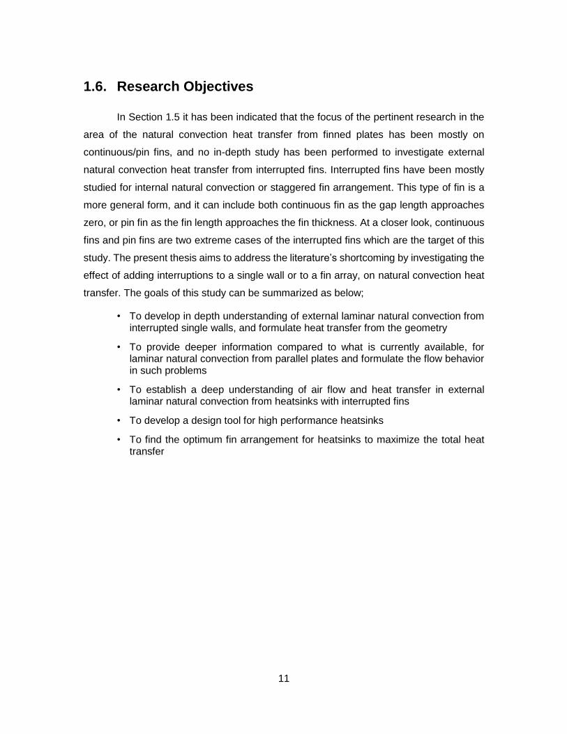
1.6. Research Objectives
In Section 1.5 it has been indicated that the focus of the pertinent research in the
area of the natural convection heat transfer from finned plates has been mostly on
continuous/pin fins, and no in-depth study has been performed to investigate external
natural convection heat transfer from interrupted fins. Interrupted fins have been mostly
studied for internal natural convection or staggered fin arrangement. This type of fin is a
more general form, and it can include both continuous fin as the gap length approaches
zero, or pin fin as the fin length approaches the fin thickness. At a closer look, continuous
fins and pin fins are two extreme cases of the interrupted fins which are the target of this
study. The present thesis aims to address the literature’s shortcoming by investigating the
effect of adding interruptions to a single wall or to a fin array, on natural convection heat
transfer. The goals of this study can be summarized as below;
• To develop in depth understanding of external laminar natural convection from interrupted single walls, and formulate heat transfer from the geometry
• To provide deeper information compared to what is currently available, for laminar natural convection from parallel plates and formulate the flow behavior in such problems
• To establish a deep understanding of air flow and heat transfer in external laminar natural convection from heatsinks with interrupted fins
• To develop a design tool for high performance heatsinks
• To find the optimum fin arrangement for heatsinks to maximize the total heat transfer

12
Chapter 2. Natural Convection from Interrupted Vertical Walls
Steady-state external natural convection heat transfer from interrupted rectangular
vertical walls is investigated in this chapter. A systematic numerical, experimental, and
analytical study is conducted on the effect of adding interruptions to a vertical plate.
COMSOL Multiphysics is used to develop a two dimensional numerical model for
investigation of fin interruption effects on natural convection. A custom-designed testbed
is built and six interrupted wall samples are machined from aluminum, and tested to verify
the numerical results. An effective length is introduced for calculating the natural
convection heat transfer from interrupted vertical walls. Performing an asymptotic analysis
and using a blending technique, a new compact relationship is proposed for the Nusselt
number. Our results show that adding interruptions to a vertical wall can enhance heat
transfer rate up to 16% and reduce the weight of the fins, which in turn, lead to lower
manufacturing and material costs.
Interruptions are discontinuities added in vertical walls to postpone the thermal
boundary layer emergence in the channel flow between two adjacent walls; thus increase
the total heat transfer rate [57]. A schematic for interrupted wall is shown in Figure 2.1. It
should be noted that this arrangement is a more general form of geometry and includes
both continuous and pin fins at the limit, where the interruption length approaches zero,
or very large values, respectively. Fin interruption is common in industry and has been
studied for internal natural convection [58] and forced convection [59]. However, as
mentioned in Section 1.5, to the author’s best knowledge, no comprehensive study is
available for natural convection from interrupted walls.
The focus of this chapter is on the effects of fin length and interruption length. To
study the natural convection heat transfer from interrupted walls, a new concept, “effective
length”, is introduced and a new compact relationship for the Nusselt number is developed
based on non-dimensional geometrical parameters.

13
Figure 2.1. Effect of interruptions on boundary layer growth in natural heat transfer from a vertical wall
2.1. Numerical Analysis
2.1.1. Governing Equations
We seek a solution for steady-state, laminar natural convection heat transfer from
an isothermal vertically-mounted interrupted wall, as shown schematically in Figure 2.1.
The conservation of mass, momentum and energy in the domain are based on assuming
a fluid with constant properties and the Boussinesq approximation [60] for density;
0u
x y
2.1
2u u P
u u gx y x
2.2
2P
ux y y
2.3
2T T
u Tx y
2.4
Fins
Fresh air entering
Thermal boundary layers
g
Fresh air entering

14
where y is the direction normal to the gravitational acceleration and x is the direction
parallel to the gravitational acceleration,u and v are the velocity in x-direction and y-
direction, respectively. Here , , and are the fluid’s density, dynamic viscosity and
thermal diffusivity, respectively.
Considering P P
x x
, where P is the ambient hydrostatic pressure, and assuming
Boussinesq approximation, Eq.2.2 yields to:
2
2( )
u u uu g T T
x y x
2.5
In our numerical simulations, the buoyancy term, ,g T T is added to the
momentum equations as a body force term. Kinematic viscosity, in Eq.2.5, is following
Boussinesq approximation and can be defined as / . Pressure inlet, with gauge
pressure set to zero, is applied to the bottom of the domain. For the top and right side of
the domain outlet boundary condition is applied, which imposes a constant pressure,
gauge pressure of zero in case of our problem. Symmetry boundary condition was chosen
for the gap region. This type of boundary condition is equivalent to a no-heat flux in the
direction normal to the boundary plane. No-slip isothermal solid surface is considered as
the boundary condition for the walls. Figure 2.2.a shows a schematic of the domain
considered for the numerical simulation, along with the chosen boundary conditions for
the fins. COMSOL Multiphysics 4.3 has been employed for mesh generation and to solve
the above-mentioned system of partial differential equations.
15
Figure 2.2. a) Schematic of the numerical domain and boundary conditions for vertical interrupted wall, b) grid used in the model for interrupted wall
2.1.2. Mesh Independency
For simulating the heat transfer in the fins, a 2D model is created in COMSOL
Multiphysics 4.3, by coupling the fluid flow and heat transfer modules. As mentioned in
Section 2.1.1, the coupling has been done by adding the Boussinesq buoyancy term to
the momentum equation. Boussinesq assumption relates the fluid density to its
temperature with a linear approximation in buoyancy term, and uses the fluid density at
ambient temperature in convective term of momentum equation. Finer grid size has been
used near the fin surface to resolve the boundary layer with enhanced accuracy.
Increasingly, coarser mesh was chosen in the regions far from the walls in order to reduce
the computational time (see Figure 2.2.b). Five different numbers of mesh elements are
used for the benchmark cases and compared in terms of average heat flux from the walls
to ensure a mesh-independent solution. The parameters chosen for the benchmark case
y
x
Isothermal walls
Symmetry
Calming
section
(a) (b)
Symmetry
Outlet
Wall
Inlet, Pin=1 atm.
t
l
G

16
are shown in Table 2.1. Accordingly, for the mesh number of approximately 45,000, we
found that the simulation gives approximately 0.01% deviation in average heat transfer
rate from walls as compared to the simulation of fins with mesh number of 65,000, while
for the number of elements less than 6,500, the model does not converge to a reasonable
solution. Figure 2.3 shows the mesh independency analysis for the benchmark case. As
the figure shows, the results are not too sensitive to the grid size, and the wall heat flux
ranges from 332.5 W/m2 for 6,500 elements to approximately 333.3 W/m2 for 68,000
elements.
Table 2.1. Parameters used in the benchmark case for numerical simulations
Parameter Description Value Unit
l Fin length 5 [cm]
G Gap length 2 [cm]
t Fin thickness 1 [cm]
T∞ Ambient temperature
20 [ᵒC]
Tw Wall temperature 60 [ᵒC]
m Number of fins 5 -
Figure 2.3. Grid independency study; walls average heat flux versus number of elements for the benchmark case (see Table 2.1)
332.5
332.7
332.9
333.1
333.3
333.5
0 10,000 20,000 30,000 40,000 50,000 60,000 70,000
Wal
ls A
ver
age
Hea
t F
lux
[W
/m2]
Number of Elements

17
The velocity and temperature domains are shown as results of the benchmark
numerical studies in Figure 2.4. As shown in the figure, the diffusion of velocity and
temperature in the gap region causes the air to reach the higher fin with higher velocity
and lower temperature. This interruption in hydrodynamic and thermal boundary layers is
the main cause for the improvement of heat transfer from the fins.
Figure 2.4. a) velocity domain, and b) temperature domain for the benchmark case; the diffusion of velocity and temperature in the gap causes the air to reach the top wall with higher velocity and lower temperature
(a) (b)
[m/s][ᵒC]

18
2.2. Experimental Study
The objective of the experimental study is to investigate the effects of interruption
length on the natural convection heat transfer from interrupted vertical walls, and also to
validate the results from numerical simulations and mathematical modeling. To achieve
this goal, a custom-made testbed is designed and built, and six interrupted wall samples
with various geometrical parameters are machined from extruded aluminum profiles. A
series of tests with different surface temperatures are conducted. The details about the
testbed design, test procedure, and uncertainty analysis are given in the proceeding
sections.
2.2.1. Testbed
The testbed is designed to measure natural convection heat transfer from
interrupted vertical walls, as shown in Figure 2.5.a. The set-up included a metal framework
from which the samples are hung, and an enclosure made of compressed insulation foam
with a thickness of 20mm to insulate the backside of the samples. Inside the foam
enclosure is filled with glass-wool to ensure the minimum heat loss from the backside of
the baseplate. As such, any form of heat transfer from the backside of baseplate is
neglected in our data analysis. The setup also includes a power supply, two electrical
heaters, attached to the backside of the baseplate, T-type thermocouples, and three Data
acquisition (DAQ) systems. Thermal paste (Omegatherm®201) is used to minimize
the thermal contact resistance between the heater and the baseplate.

19
Figure 2.5. a) schematic and photo of the testbed; b) backside of the samples; positioning of the thermocouples and heater
Six heatsink samples with the same baseplate width but different fin and
interruption lengths are prepared by machining extruded aluminium profiles. To fully
investigate the effects of thermal boundary layer growth, different dimensions of the fins
and interruptions are chosen, as listed in Table 2.2.
Table 2.2. Dimensions of the interrupted wall samples used in experimental study
Sample name # l [mm] m G [mm] L [m] G/l l/t
SW-1 50 14 50 1.35 1 5
SW-2 50 7 150 1.25 3 5
SW-3 50 10 100 1.40 2 5
SW-4 50 5 300 1.45 6 5
SW-5 50 10 150 1.85 3 5
SW-6 50 17 25 1.47 0.5 5
Note: The baseplate length is shown with L, and all the samples share baseplate width, W = 101 mm, fin height, H = 100 mm, and fin thickness, t = 10 mm.
(a) (b)
HeatersT4
T3
T2
T1Tamb
V
T8
T7
T6
T5
L
W
T9
T10Power Supply
I

20
2.2.2. Test Procedure
The experiments are performed in a windowless room with an environment free of
air currents. The room dimensions are selected to be large enough to ensure constant
ambient temperature during the test. The input power supplied to the heaters is monitored
and surface temperatures are measured at various locations at the back of the baseplate.
Electrical power is applied using a variable voltage transformer (Variac SC-20M), and
using DAQ systems (National Instruments, NI9225 and NI9227), the voltage and the
current are measured to determine the power input to the heater. Eight self-adhesive,
copper-constantan thermocouples (Omega, T-type) are installed in various vertical
locations on one side of the baseplate, as shown in Figure 2.5.b. Two extra thermocouples
are installed on the same level with the highest and lowest thermocouples to make sure
that the temperature is well distributed horizontally (9T and
10T in Figure 2.5.b). All
thermocouples are taped down to the backside of the samples baseplate to prevent
disturbing the buoyancy-driven air flow. One additional thermocouple is used to measure
the ambient temperature during the experiments. Thermocouples are plugged into a DAQ
system (National Instruments, NI9213). Temperature measurements are performed at ten
points in order to monitor the temperature variation on the wall, and the average is taken
as the baseplate temperature. Among all the experiments, the maximum standard
deviation from the average temperature is 4˚C. Since the experiments are performed to
mimic the uniform wall temperature boundary condition, the thickness of the baseplate
and the fins are selected fairly high (10mm) to ensure the minimum thermal bulk resistance
and uniform temperature distribution in the samples. An infrared camera (FLIR, SC655) is
used to observe the temperature difference between the baseplate and the fins. The
maximum measured difference between the fins and the baseplate is about 2˚C, so for
the data reduction, the fins are assumed to be at the same temperature with the baseplate.
For each of the six samples, the experimental procedure is repeated at various power
inputs. The baseplate temperature, wT , the ambient temperature,T , and the heater
power, ,inputp are recorded at steady-state considering the power factor equals one. Table
2.3 lists the range of some important test parameters. The steady-state condition is
considered to be achieved when the rate of all temperature variations is less than 0.1˚C/hr,
which on average, takes 240 minutes from the start of the experiment.

21
Table 2.3. Range of important parameters in the experimental study
Parameter Description Range Unit
m Mass of the samples 1.2-2.1 [kg]
P Heater power 30-150 [W]
T Ambient temperature 20-22 [ᵒC]
wT Wall temperature 35-75 [ᵒC]
lRa Rayleigh number 105-108 -
For the data reduction, natural convection from the baseplate and fin tips are
calculated using the available correlations in literature [19], and subtracted from total heat
input to the system. Following Rao et al. [61], the effect of radiation heat transfer is also
subtracted from the fins’ total heat transfer (see Appendix B). Due to relatively low surface
temperature and low emissivity of machined aluminum (between 0.09 and 0.1), the effect
of radiation is not significant. The maximum calculated value for radiation heat transfer is
4.2% of total heat transfer from the sample.
2.2.3. Uncertainty Analysis
Voltage ,V and current ,I are the electrical parameters measured in our
experiments, from which the input power ,P can be calculated (see Eq.2.6). The overall
accuracy in the measurements is evaluated based on the accuracy of the measuring
instruments, mentioned in Section 2.2.2. The accuracy of the voltage and current readings
are 3% for both parameters, based on suppliers’ information. The reported accuracy
values are given with respect to the instruments readings, and not the maximum range of
measurement. The maximum uncertainty for the measurements can be obtained using
the uncertainty analysis method provided in [62]. To calculate the uncertainty with the
experimental measurements the following relation is used [62]:
12 2
R i
i
R
x
2.6

22
where R is the uncertainty in the general function of 1 2( , ... ),nR x x x and i is the uncertainty
of the independent variable .ix The final form of the uncertainty for the input power
becomes;
P V I 2.7
12 2 2P V I
P V I
2.8
12 2 2 2 2 2
.
.
4 4Rad w
wRad
Q T T l H t
T T l H tQ
2.9
. . .[ ]N C RadQ W P Q 2.10
Substituting the values for , , , , , ,wV I T T l H and t into Eqs. 2.8 and 2.9, the maximum
uncertainty value for NCQ is calculated to be 8%. The measured temperature uncertainty
T is 1 C . To calculate the heat transfer coefficient from measured . .N CQ and T , Eq.
2.11 can be used
. .N CQ
hA T
2.11
so;
12 22 2 2 2
. .
. .
w N C
w N C
h T T l H Q
h T T l H Q
2.12
For the calculation of Nusselt number, effective length, .,effL is used as the
characteristic length, and since it is not measured, .effL is not included in uncertainty
analysis. Thermophysical properties such as thermal conductivity of air are also assumed
to be constant. Table 2.4 shows a list of parameters used in the uncertainty analysis with
their calculated value. The amount of uncertainty for Nusselt number, which is calculated
to be 10%, is shown as error bars on experimental data.
23
Table 2.4. The uncertainty analysis parameters
Parameter Maximum uncertainty
V V 0.3%
I I 0.3%
P P 0.4%
T ±1[˚C]
H 0.1 [mm]
l 0.1 [mm]
t 0.1 [mm]
. .Rad RadQ Q 7.5%
. . . .N C N CQ Q 8%
2.3. Results and Discussion
In this section, a new concept called “effective fin length” is introduced to calculate
the Nusselt number for the natural convection heat transfer along the interrupted vertical
fins. The effective length is obtained through equating the heat transfer rate from the actual
interrupted wall with an imaginary continuous vertical wall, with the length of ..effL Natural
convection heat transfer from an isothermal vertical wall is a well-known subject in the
literature and can be calculated from the following relationship [63]:
. .
1
40.59eff effL LNu Ra
2.13
knowing that
.
.
eff
eff
L
h LNu
k 2.14
substituting . .N CQh
A T
into Eq. 2.14 and using Eq. 2.14, one can find;

24
12 52
2
0.59eff
QL T
k g
2.15
we also introduce and , as follows;
l
t 2.16
G
l 2.17
In order to develop a general model for all ranges of , two asymptotes are
recognized and a blending technique [64] is implemented to develop a compact
relationship for the effective length and the corresponding Nusselt number. The first
asymptote is developed for small values of , where 0, for which the flow behaviour
resembles the flow over a vertical wall that has no interruptions with a total length of
L ml 2.18
where m is the number of fin rows. For the first asymptote, 0, the effective length is
correlated using the present numerical results.
., 0
0.22 1effL
ml
2.19
The second asymptote is when , which is the limiting case where the fins are
located far enough from each other and they act as an individual single wall. In other
words, each fin’s flow/heat transfer pattern will not get affected by the fins located at the
bottom. For this asymptote, , Eqs. 2.20 to 2.23, available in literature [16,65], are
used to calculate the heat transfer from the wall. Natural convection heat transfer from the
walls in this asymptote is the summation of heat transfer from all sides of the fin (bottom,
two sides and the top surface). The relationships used for calculating the heat transfer
from the top, bottom, and sides of the wall are given in [66].
total ends sidesQ Q Q 2.20
1
40.59sides l lNu Nu Ra 2.21

25
1
40.56top tNu Ra 2.22
1
40.27bottom tNu Ra 2.23
Natural convection heat transfer, calculated from the above equations, should be
substituted in Eq. 2.15 to give the .effL for larger values of , i.e. ., .effL As a result, for the
top, bottom and sides of the wall, we can calculate the ratio of . /effL ml as:
43 3
1 4., 3
10.83 1
effLm
ml
2.24
Having ,effL and , 0effL known, a compact relationship for effL can be developed
using a blending technique, introduced by Churchill and Usagi [64];
1
, 0 ,
c c c
eff eff effL L L
2.25
where c is a fitting parameter, and its value is found by comparison with the present
numerical data; the best fit is found for 3.c This fitting parameter is found by minimizing
the maximum difference between the model and the numerical data.effLNu is calculated by
substituting effL into Eq. 2.14. The final relationship is a function of, , , ,m and Ra , which in
turn, is a function of temperature difference, as shown below:
.
11 44
31 3 4
3. 4 41
0.59 0.22 1 0.83 1 ,5 15eff
eff
L l
hLNu Ra m m
k
2.26
where l is the fin length, is the aspect ratio of the fin, m is the number of fin rows, andlRa
is the Rayleigh number based on fin length.
Figure 2.6 shows the asymptotic behaviour of the natural convection from
interrupted vertical walls for the two discussed limiting ranges of . Two different trends

26
can be seen in the present data, for the extreme values of . The first trend shows small
values of , related to a long vertical wall, the region in which the data collapses into a
straight line. The second trend corresponds to very large values of , related to a short fin
with . ,effL l where the data approaches a horizontal asymptote.
Figure 2.6. Heat transfer versus /G l for different /l t values. The figure also
shows the comparison between the numerical data (symbols) and introduced asymptotes (Lines).
Figure 2.7 shows dimensionless form of the proposed effective length, calculated
using numerical data, as a function of . Asymptotic behavior of the effective length can
be observed in the numerical data. We developed a new compact correlation for the
effective length using the blending technique [64] as follows;
1.0
1.5
2.0
2.5
3.0
3.5
4.0
4.5
5.0
5.5
0 20 40 60 80 100
Q/
ml
[W/m
]
κ =G/l
ζ = 10
ζ = 15
κ → 0
ζ = 7.5
ζ = l/t
κ → ∞
ζ = 5
t
l
G
g

27
13 33
3 41 4
3. 31
0.22 1 0.83 1effL
mml
2.27
Figure 2.7. Effective length versus /G l for different /l t values. The figure
also shows the comparison between the numerical data (symbols) and the proposed correlation (lines) for the effective length.
To calculate the Nusselt number from the numerical data, the average wall heat
flux is obtained from the numerical simulations and having the wall and ambient
temperature, the heat transfer coefficient is calculated. Using the heat transfer coefficient,
the calculated effective length, and thermal conductivity of the air, the numerical Nusselt
number is calculated. This allows developing a new compact correlation for Nusselt
number based on the effective length, characterizing the natural convection heat transfer
from interrupted vertical walls (Eq. 2.26). This Nusselt number can be used to calculate
the heat transfer rate for any rectangular interrupted fin in the range of 5 15. The
0
0.5
1
1.5
2
2.5
3
3.5
4
0.1 1 10 100
Lef
f. /(
ml)
κ =G/l
ζ = 5
ζ = 7.5ζ = 10
ζ = 15
Leff./m.l = 0.22 κ + 1
κ → 0
t
l
G
g
κ → ∞

28
parameter /l t represents the aspect ratio or slenderness of the fins. For / 5,l t the fin
geometry will become closer to a cuboid/pin fin and the correlations used to calculate the
heat transfer are no longer valid. Also for / 15l t , the fins will be too long and the effect of
fin thickness will be negligible. The effect of fin thickness is considered in our calculations
and appears in Eqs. 2.26 and 2.27.
In Figure 2.8, the experimental data obtained from the interrupted vertical wall
samples, is compared against the proposed new relationship for the Nusselt number Eq.
2.26. Figure 2.8 also shows that the numerical simulation results are in very good
agreement with experimental data. As can be seen, the proposed compact relationship is
in very good agreement with both experimental and numerical results. The average
relative difference between the proposed correlation and the experimental data is
approximately 9% and the maximum relative difference is 15%.
Figure 2.8. Nusselt number versus /G l for different /l t values. The figure
also shows the comparison between the numerical data (hollow symbols), experimental data (solid blue symbols), and the proposed compact relationship (lines)
0
5000
10000
15000
20000
25000
0.1 1 10 100
Nu
Lef
f.
κ =G/l
ζ = 7.5
ζ = 10
ζ = 15
ζ = 5
t
l
G
g
ζ ↑ κ → ∞κ → 0

29
2.4. Conclusion
Experimental, numerical and analytical studies were performed to develop a
compact correlation for natural convection heat transfer from vertical interrupted walls.
The effects of interruption length in natural convection were thoroughly investigated. A
comprehensive numerical modeling was performed using COMSOL Multiphysics. A
custom-designed testbed was built and six aluminum interrupted wall samples were
prepared and tested to verify the developed numerical and analytical models over the
entire range of interrupted fin parameters. The collected data were successfully compared
with the present numerical and analytical models. A new compact relationship was
developed for the Nusselt number for natural convection heat transfer from interrupted fins
using a blending technique, based on the non-dimensional geometrical parameters
/G l and / .l t This relationship can be used for calculating heat transfer rate for any
rectangular interrupted fin in the range of 5 15. The comparison of our experimental
data to the available data in the literature [63], shows that with the similar baseplate
dimensions, adding interruption to a single wall can improve the heat dissipation up to
16% compared to a continuous vertical wall.

30
Chapter 3. Natural Convection from Vertical Parallel Plates
Steady-state external laminar natural convection heat transfer from isothermal
vertical parallel fins is modeled analytically in this chapter. Integral technique is used to
solve the governing equations. Compact relationships are developed for the velocity and
temperature profiles for the buoyancy-driven channel flow for100 4500lRa range.
Comprehensive numerical and experimental studies are performed, and the proposed
analytical model is successfully validated against the numerical data with the maximum
relative differences of 9.8% and 3.5% for velocity and temperature profiles, respectively.
Also new closed-form correlation for local and average Nusselt numbers, as functions of
Rayleigh number, temperature difference and fin aspect ratio are reported, and validated
against the experimental data with 1.6% maximum relative difference.
3.1. Problem Statement
The main objective of this study is to develop a compact, analytical model that can
predict the natural convection heat transfer from a squared array of vertically-mounted
rectangular isothermal fins (see Figure 3.1). Figure 3.1.b schematically shows the front
view of the considered geometry for two fins in the fin array. Due to symmetry, only one
channel is needed to represent the entire fin array. The assumptions used in this study
are listed below;
• Steady-state 2D heat transfer and fluid flow (fins are assumed long enough in the direction normal to the surface)
• Laminar flow
• Isothermal walls, atwT
• Constant thermo-physical properties, except for the fluid density
• Boussinesq approximation for change of density as function of temperature [60].

31
It is assumed that the fin height in z-direction is large enough that the effects of
baseplate can be neglected and the problem can be treated as a two dimensional flow.
Figure 3.1. a) a naturally-cooled enclosure of a power converter; b) schematic of the heatsink, and c) solution domain, selected as the control volume
3.1.1. Governing Equations and Boundary Conditions
Integral technique is used to solve the governing equations subjected to constant
wall temperature boundary conditions. Integral technique is a powerful analysis method
developed by Pohlhausen and Von Karman in the first decade of twentieth century to
obtain approximate solutions to complex problems [60]. It works based on the principle
that the general behavior of the velocity and temperature profiles are known. Assuming a
(c)
(a)
(b)
s
W
L
H

32
profile for each, and satisfying conservation of mass, momentum, and energy in a lumped
fashion across the region of interest, we can obtain velocity and temperature profiles within
an acceptable accuracy by satisfying the boundary conditions. The conservation laws can
be written for the control volume shown in Figure 3.1.c. Table 3.1 summarizes the integral
form of momentum and energy balance equations for the considered integral control
volume. To find more details about the methodology to obtain the governing equations
from the control volumes shown in Table 3.1, readers are invited to see Appendix A. The
conservation equations are subjected to the following boundary conditions;
at 0y ( , 0) ( , 0)
0u x T x
y y
3.1
at / 2y s ( , ) 0 ( , )2 2
w
s su x and T x T 3.2
at 0x (0, ) ( ) (0, )inu y u y and T y T 3.3
as x . .( , ) ( ) ( , )F D wu x y u y and T x y T 3.4
Equation 3.1 is concluded from the symmetry at the centerline of the channel. The
parameter ( )inu y represents the velocity profile at the channel inlet and will be discussed
later in Section 3.2.1. It should be noted that the velocity at the channel inlet cannot be
zero, since the velocity has a non-zero profile at the channel outlet, and conservation of
mass implies that the velocity should have a non-zero profile in the inlet.

33
Table 3.1. Integral form of conservation equations for the integral control volume
Equation Schematic of C.V. Terms description Conservation equation
Momentum
/2
2
0
/2
0
( , )
( , )
s
w
s
u x y dyx
g T x y T dy
Energy
Note: The buoyancy and weight forces are written for the unit depth.
3.2. Present Solution
The first step, before solving the governing equations, is to determine the velocity
profile at the inlet of the channel, 0x (Eq. 3.3). The following section presents the details
on how ( )inu y can be obtained.
3.2.1. Entrance Velocity
To find the velocity profile at 0,x conservation of mass can be written for a
control volume enclosing the entire domain between the fins, as shown in Eq. 3.5. If the
channel is long enough so that the velocity reaches fully-developed condition, the fluid
temperature will be equal to the wall temperature [60]. Since the cross section area is
M
/2
2
0
2 ( , )
s
x u x y dy
M
/2
2( )
0
/2
2
0
2 ( , )
(2 ( , ) )
s
x dx
s
u x y dy
u x y dyx
/2
0
2 ( , ) ( , )
s
x pE c u x y T x y dy /2
0
( , ) ( , )s
w
p
u x y T x y dyx
q
c
/2
( )
0
/2
0
2 ( , ) ( , )
(2 ( , ) ( , ) )
s
x dx
s
p
p
E c u x y T x y dy
c u x y T x y dyx

34
constant and fluid enters the channel with the ambient temperature, mass balance can be
written as:
. .( ) ( )w
F D inT Tu y u y
3.5
The fully-developed velocity profile at the outlet of parallel fins is known [60];
2 2
. . 2
4( ) 1
8F D
g Ts yu y
s
3.6
Equation 3.5 is the conservation of mass between the inlet and outlet of the
channel. To find the density at the outlet which is assumed to be at the wall temperature,
a linear approximation can be used similar to the assumption made in Boussinesq
approximation;
( ) 1T T T 3.7
Substituting wT forT in Eq. 3.7 and substituting the result in Eq. 3.5, ( )inu y can be
found as;
2 2
2
1 4( ) 1
8in
T Tg s yu y
s
3.8
Now, all the boundary conditions are known, and integral technique can be
implemented to find the velocity and temperature profiles in the channel, as discussed in
the following section.
3.2.2. Integral Technique
A second order polynomial in the y-direction is assumed for both temperature and
velocity profiles;
2
1 1 1( , ) ( ) ( ) ( )u x y a x y b x y c x 3.9
2
2 2 2T( , ) ( ) ( ) ( )x y a x y b x y c x 3.10
Applying the boundary conditions in the y-direction (Eqs. 3.1 and 3.2), into Eqs.
3.9 and 3.10, we will have;

35
2
2( , ) ( )4
su x y f x y
3.11
2
2( , ) ( )4
w
sT x y g x y T
3.12
Both ( )f x and ( )g x are unknown functions to be found, and can be interpreted as
the velocity and temperature at the centerline of the channel along the x-direction. Physics
of the flow and heat transfer suggest that both velocity and temperature at centerline would
increase rapidly at the beginning of the channel (entry region), and approach an
asymptotic value as the fluid moves along the x axis (fully developed flow). Using similarity
solution technique for buoyancy-driven flow, Sparrow and Gregg [67,68] showed the
temperature variation that gives rise to a similarity in the laminar boundary layer governing
equations is either a power law or exponential distributions. Similar assumptions have
been made by Gebhart et al. [69,70] for solving natural convection heat transfer equations
in buoyancy induced flow over an adiabatic vertical surface and laminar natural convection
plume above a horizontal line heat source. Therefore, a general exponential behavior can
be assumed for ( )f x and ( )g x , as follows:
2
( )4
xsf x e 3.13
2
g( )4
x
w
sx e T 3.14
where , , , , , and are constants that should be determined. The coefficient
2 / 4s in Eqs. 3.13 and 3.14 and wT in Eq. 3.14, are added for convenience and have no
effect on the generality of the solution. Having Eq. 3.8, substituting Eqs. 3.13 and 3.14 into
Eqs. 3.11 and 3.12, and applying the boundary conditions in the x-direction, the
parameters , , , and will be determined as bellow;
21
8
g Ts
3.15
2 2 21
8
g T s
3.16
wT 3.17
T 3.18

36
Substituting the above calculated constants in Eqs. 3.11 and 3.12 and solving the
integrated energy and momentum equations (Table 3.1), the two remaining constants,
and can be obtained. After some mathematical manipulations, the velocity and
temperature domain can be determined in the form of Eqs. 3.19 and 3.20.
2 2
2 4 3
40 3 4 2
1 2 , e 1
44
T T x
g s T Tg su x y y
TT
3.19
4
1202
1 2
2
4, e
4
x
g Ts Tw
T sT x y y T
s
3.20
Eqs. 3.19 and 3.20 can be presented in a more compact form, after non-
dimensionalizing by introducing the dimensionless parameters shown in Table 3.2.
Table 3.2. Dimensionless parameters
Parameter Description
X /x l
Y /y s
U /u s
/w wT T T T
/l s
Pr /
sGr 3 2/g T s
sRa PrsGr
Using dimensionless parameters, the velocity and temperature distribution inside
the channel can be presented as;
3160 1
4
1 21 1, 1 e
4 4s
TX
GrT TsU X Y Ra T Y
3.21

37
2 1, 4exp 120
1 4s
XX Y Y
Ra T
3.22
3.3. Numerical Simulation
In order to validate the present analytical model, an independent 2-dimensional
numerical model of the problem is developed in the commercially available software
package, ANSYS FLUENT 14.0. In order to couple the momentum and energy equations
and add the buoyancy effects to the simulation, Boussinesq approximation is imposed to
the air density behavior as a function of temperature, and gravity effect is added to the
domain as body force in negative y-direction. Figure 3.2.a shows a schematic of the
domain considered for the numerical simulation, along with the boundary conditions
assumed for the channel. Inlet atmospheric pressure and constant temperature, ,T T is
applied at the bottom of the domain as the boundary condition. For the top of the domain,
outlet pressure boundary condition is applied which imposes the pressure to be
atmospheric pressure. No-slip, isothermal solid surface ( 0 wu and T T ) is considered for
the walls, and symmetry boundary condition is assumed for the centerline, which imposes
no momentum and heat transfer, in the direction normal to the boundary. The parameters
used for the benchmark case are shown in Table 3.3.

38
Figure 3.2. a) schematic of the numerical domain and boundary conditions, b) the grid used in the model, c) velocity domain, and d) temperature domain for the benchmark case
Table 3.3. Parameters used for the numerical simulation benchmark
Parameter Description Value Unit
l Wall length 10 [cm]
s Wall spacing 8 [mm]
T Ambient temperature 20 [ᵒC]
wT Wall temperature 60 [ᵒC]
sRa Rayleigh number 1700 -
To ensure a mesh independent solution, different grid sizes were tested and total
heat transfer rate from the fins was chosen as monitoring parameter. Figure 3.3 shows
the mesh independency analysis for the benchmark case. For the mesh number of
approximately 900, we found that the simulation gives approximately 0.85% deviation in
average heat transfer rate from walls compared to the simulation with mesh number of
3000, while for the number of elements less than 900 the model does not converge to a
reasonable solution. The relative deviation for average wall heat flux, is 0.20%, 0.05%,
Calming section
Symmetry
Outlet
Inlet
No-slip,
isothermal wall
Symmetry
(a)
(b)
(c) (d)
[m/s] [k]

39
0.02%, 0.01%, and 0.00% for 10,000, 20,000, 30,000, 40,000, and 50,000 number of
elements, respectively. Consequently, 40,000 elements is chosen for numerical
simulations. As shown in Figure 3.2.b, finer grid size is used at the vicinity of the solid wall
to resolve the boundary layer effects with higher accuracy. The maximum skewness,
calculated based on the equilateral volume method, was 0.21 which assures high quality
of the grid. A sample of velocity and temperature domains are shown as results of the
numerical studies in Figure 3.2.c and Figure 3.2.d.
Figure 3.3. Grid independency study; walls average heat flux versus number of elements for the benchmark case (see Table 3.3)
3.4. Experimental Study
A custom-made testbed is designed and built, in order to validate the results from
integral solution and numerical simulations. Five samples, with various fin spacing are
prepared, and a series of tests with different surface temperatures are conducted.
252
252.5
253
253.5
254
254.5
255
255.5
256
0 10000 20000 30000 40000 50000 60000 70000
Aver
age
Wal
l H
eat
Flu
x [
W/m
2]
Number of Elements

40
3.4.1. Testbed
A custom-made testbed is designed for measuring natural convection heat transfer
from the finned heatsinks, as shown in Figure 3.4. The set-up includes an enclosure made
of Plexiglas (PMMA) which is insulated by a layer of foam with a thickness of 20 mm. The
testbed also includes 20 cm long 150 W Chromalox strip heaters which are attached to
the backside of the fins baseplate, and a data acquisition system, supplied by National
Instruments (NI DAQ Chassis). High conductive thermal paste provided by Omega is used
to decrease the thermal contact resistance between the heater and the samples
baseplate. The voltage and the current of the supplied power are measured with an Agilent
34405A digital multimeter.
Five samples with the same baseplate size, and different fin spacing s and fin
height ,H are prepared. Dimensions of the finned plate samples are given in Table 3.4.
Table 3.4. Dimensions of the finned plate samples
Sample # s [mm] n H [mm] l [mm]
1 9.5 8 17 300
2 6.0 12 17 300
3 14.0 6 17 300
4 9.5 8 10 300
5 9.5 8 25 300
Note: Baseplate width is similar in all samples, W= 101 mm.

41
Figure 3.4. a) schematic of the test-bed; b) samples dimensions, heater and thermocouples positioning; c) testbed casing and insulation; and d) a photo of the testbed
Insulator
Heatsink
Thermocouples
DAQ
(a)
T1
T2
T3
T4
T5
T∞
10 cm
2 cm
30 cm
3 cm
8 cm
Heater
(b)Plexiglas casing
Fins
Insulation
foam
(c) (d)

42
3.4.2. Uncertainty Analysis
Uncertainty analysis for the experimental study on continuous fin heatsinks is very
similar to what performed in Section 2.2.3. Equations 2.6 to 2.10 are directly used for the
uncertainty analysis of the experimental study. Table 2.4 is also valid to be used for the
current experiments. Performing the uncertainty analysis for the Nusselt number, the
maximum uncertainty value for sNu is calculated to be 4%. The measured temperatures
uncertainty T is 2 ,C which is twice as the accuracy of the thermocouples. The
calculated uncertainties forsNu is reported as error bars in the experimental results.
3.5. Results and Discussion
Figure 3.5 shows the comparison between the numerical results and the analytical
solution. Equations 3.21 and 3.22, are used for the velocity and temperature distributions
at different cross sections along the x-direction. As shown, at the entrance of the channel,
because of a sudden jump in temperature and velocity in the y-direction due to the effects
of wall, the integral technique cannot precisely predict the temperature and velocity
profiles. This is an expected shortcoming of the integral technique, and it happens
because a smooth continuous functions is used for both temperature and velocity
distributions over the entire domain and these profiles cannot completely conform to the
sudden changes in the flow characteristics at the entrance region. However, the
agreement between the numerical data and analytical model improves at regions farther
from the entrance region. Neglecting the entrance of the channel, 0.01 /sx Ra [71],
the maximum relative difference for the velocity and temperature distribution between the
analytical solution and the numerical simulation are 9.8% and 3.5%, respectively.

43
Figure 3.5. Comparison between the analytical solution (lines), a) velocity b) temperature distribution and numerical results (symbols) at various cross sections along the channel
0
0
0
0
0
0
0
0
0
0.0 0.1 0.2 0.3 0.4 0.5 0.6
U=
us/α
(x1
0-4
)
Y=y/l
X=x/l
3160 1
4
1 21 1, 1 e
4 4s
TX
GrT TsU X Y Ra T Y
X=0
X=0.2 to 1
(a)
1
2
5
3
4
6
7
8
2 1, 4exp 120
1 4s
XX Y Y
Ra T
0.0
0.2
0.4
0.6
0.8
1.0
1.2
0.0 0.1 0.2 0.3 0.4 0.5 0.6
θ=
(Tw-T
)/(T
w-T∞)
Y=y/s
X=x/l
X=0
X=0.2
X=0.4
X=0.6
X=0.8
X=1
(b)
2 1, 4exp 120
1 4s
XX Y Y
Ra T
0.0
0.2
0.4
0.6
0.8
1.0
1.2
0.0 0.1 0.2 0.3 0.4 0.5 0.6
θ=
(Tw-T
)/(T
w-T∞)
Y=y/s
X=x/l
X=0
X=0.2
X=0.4
X=0.6
X=0.8
X=1
(b)
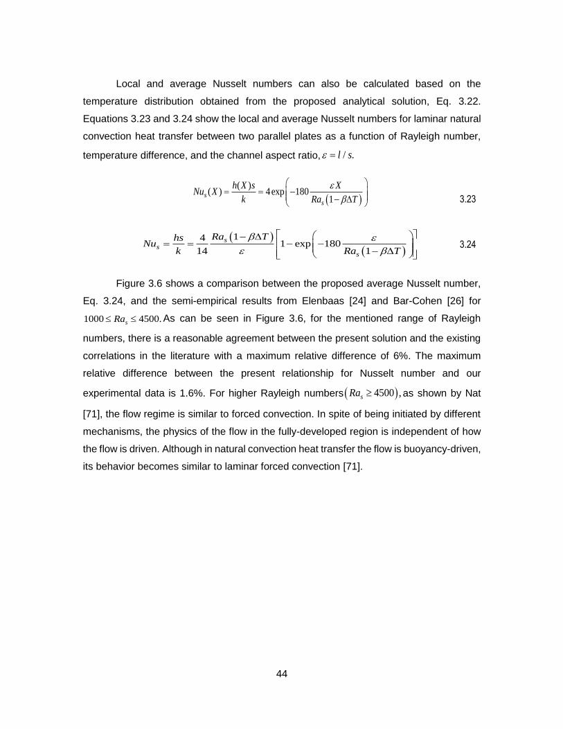
44
Local and average Nusselt numbers can also be calculated based on the
temperature distribution obtained from the proposed analytical solution, Eq. 3.22.
Equations 3.23 and 3.24 show the local and average Nusselt numbers for laminar natural
convection heat transfer between two parallel plates as a function of Rayleigh number,
temperature difference, and the channel aspect ratio, / .l s
( )
( ) 184exp 01
ss
h X s XNu X
k Ra T
3.23
141 exp 180
14 1
ss
s
Ra ThsNu
k Ra T
3.24
Figure 3.6 shows a comparison between the proposed average Nusselt number,
Eq. 3.24, and the semi-empirical results from Elenbaas [24] and Bar-Cohen [26] for
1000 4500.sRa As can be seen in Figure 3.6, for the mentioned range of Rayleigh
numbers, there is a reasonable agreement between the present solution and the existing
correlations in the literature with a maximum relative difference of 6%. The maximum
relative difference between the present relationship for Nusselt number and our
experimental data is 1.6%. For higher Rayleigh numbers 4500 ,sRa as shown by Nat
[71], the flow regime is similar to forced convection. In spite of being initiated by different
mechanisms, the physics of the flow in the fully-developed region is independent of how
the flow is driven. Although in natural convection heat transfer the flow is buoyancy-driven,
its behavior becomes similar to laminar forced convection [71].

45
Figure 3.6. Comparison between the present average Nusselt number, existing semi-empirical relations in the literature [24] and [26], and our experimental data
3.6. Conclusion
A new analytical solution for steady-state natural convection from isothermal
parallel plates is presented. New compact analytical relationships are developed for
velocity and temperature distributions for the buoyancy-driven channel flow. Integral
technique is used in combination with power law assumption in the presented analytical
solution. An independent numerical simulation is performed using commercial software
package, ANSYS FLUENT, for validation purposes. A custom-made testbed is built and
five different aluminum heatsinks are prepared and tested to validate the numerical and
analytical results. The proposed temperature and velocity profiles are compared to the
numerical simulations results and good agreement is observed. For the first time, an
analytical compact model is proposed for calculating the local Nusselt numbers in natural
convection heat transfer from parallel plates, which is successfully validated by
experimental data.
1.0
1.5
2.0
1.E+03 2.E+03 3.E+03 4.E+03 5.E+03
Nu
s
Ras
Present solution
Elenbaas [18]
Bar-cohen [19]
Experimental data
111 exp 120
30 1
ss
s
Ra TNu
Ra T
3
41 351 exp
24s s
s
Nu RaRa
0.522
0.25
24 1
0.59 s
s s
NuRa Ra
(1942)
(1984)

46
Chapter 4. Natural Convection from Interrupted Fins
The focus of this chapter is on the design of high performance naturally-cooled
heatsinks with vertical rectangular interrupted fins. A systematic analytical approach is
taken, to solve the governing equations of the air flow and heat transfer from the heatsink.
Closed-form correlations are presented for temperature and velocity distribution, and an
easy-to-use method is introduced to design such heatsinks. Numerical simulations are
used to provide better understanding of the physics of flow and heat transfer mechanism.
An extensive experimental study is also conducted to verify the results from analytical
solution and numerical simulation. Results show that the new-designed heatsinks are
capable of dissipating heat around five times more than currently available naturally-
cooled heatsinks, with weight up to 30% lighter. The new heatsinks can increase the
capacity of passive thermal management systems significantly.
4.1. Problem Statement
The objective of this chapter is to develop an analytical model that can predict the
natural convection heat transfer from a square array of vertical rectangular isothermal fins.
Figure 4.1 schematically shows the fins arrangement, parameters used to define the
geometry, and control volumes used to model the heat transfer. To solve the problem,
the domain is divided into multiple sub-domains, containing the channels made by two
adjacent columns of fins, and the gaps region between two fin rows. The effects of
neighboring channels on each other are neglected, so the problem is only solved between
two fin columns and then the solution is extended to the whole domain. The problem is
divided into two parts; i) channel flow which contains the region between two neighboring
fins, and ii) gap flow which is related to the void region between two rows of fins. Each
part is solved separately, and the solution of each part is superposed to solve the whole
domain.

47
Figure 4.1. A schematic of heatsink with interrupted fins, geometrical parameters used to address fin parameters, and the regions related to channel flow and gap flow
4.2. Solution Methodology
As shown in [55] and [57], adding interruption to a fin array will force the boundary
layer to reset and increase the heat flux from the fins; however, cutting fins to add
interruptions will result in losing surface area, which leads to a decrease in total heat
transfer from the heatsink. In order to consider these two competing trends in our heatsink
W
s
G
L
H
g
Gap flow
Channel flow
ttb
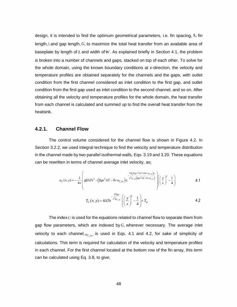
48
design, it is intended to find the optimum geometrical parameters, i.e. fin spacing, ,s fin
length, ,l and gap length, ,G to maximize the total heat transfer from an available area of
baseplate by length of L and width of .W As explained briefly in Section 4.1, the problem
is broken into a number of channels and gaps, stacked on top of each other. To solve for
the whole domain, using the known boundary conditions at x-direction, the velocity and
temperature profiles are obtained separately for the channels and the gaps, with outlet
condition from the first channel considered as inlet condition to the first gap, and outlet
condition from the first gap used as inlet condition to the second channel, and so on. After
obtaining all the velocity and temperature profiles for the whole domain, the heat transfer
from each channel is calculated and summed up to find the overall heat transfer from the
heatsink.
4.2.1. Channel Flow
The control volume considered for the channel flow is shown in Figure 4.2. In
Section 3.2.2, we used integral technique to find the velocity and temperature distribution
in the channel made by two parallel isothermal walls, Eqs. 3.19 and 3.20. These equations
can be rewritten in terms of channel average inlet velocity, as;
2,
2 2, ,
5ν T 24
2β 8 2 2
,
1 1 β β 8 e
4 ( , )
4
C in
C in C in
g s u x
s u gs T u
C C inx yy
u g Ts gs T us
4.1
2
,
15α2
1, 4) e
4( C in
x
s uC w
yT T Tx y
s
4.2
The indexC is used for the equations related to channel flow to separate them from
gap flow parameters, which are indexed by ,G wherever necessary. The average inlet
velocity to each channel,, ,C inu is used in Eqs. 4.1 and 4.2, for sake of simplicity of
calculations. This term is required for calculation of the velocity and temperature profiles
in each channel. For the first channel located at the bottom row of the fin array, this term
can be calculated using Eq. 3.8, to give;
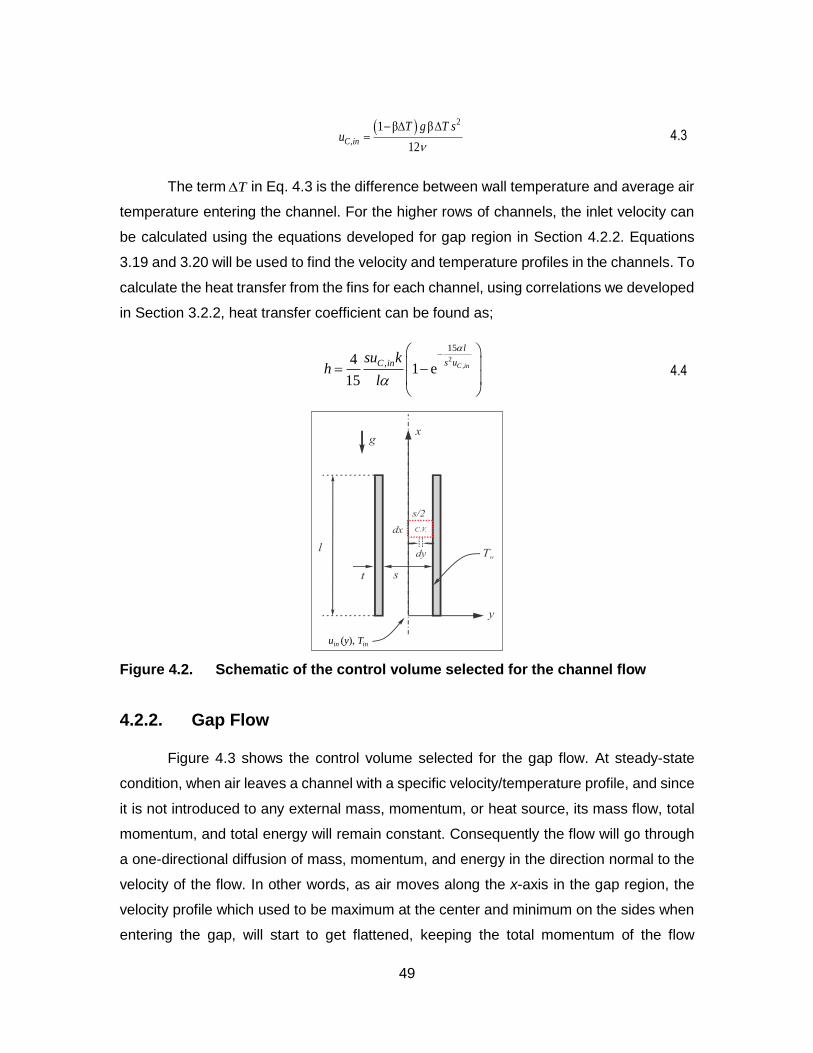
49
,
21 β β
12 C in
T g T su
4.3
The term T in Eq. 4.3 is the difference between wall temperature and average air
temperature entering the channel. For the higher rows of channels, the inlet velocity can
be calculated using the equations developed for gap region in Section 4.2.2. Equations
3.19 and 3.20 will be used to find the velocity and temperature profiles in the channels. To
calculate the heat transfer from the fins for each channel, using correlations we developed
in Section 3.2.2, heat transfer coefficient can be found as;
2
,
15
,41 e
15
C in
l
s uC insu kh
l
4.4
Figure 4.2. Schematic of the control volume selected for the channel flow
4.2.2. Gap Flow
Figure 4.3 shows the control volume selected for the gap flow. At steady-state
condition, when air leaves a channel with a specific velocity/temperature profile, and since
it is not introduced to any external mass, momentum, or heat source, its mass flow, total
momentum, and total energy will remain constant. Consequently the flow will go through
a one-directional diffusion of mass, momentum, and energy in the direction normal to the
velocity of the flow. In other words, as air moves along the x-axis in the gap region, the
velocity profile which used to be maximum at the center and minimum on the sides when
entering the gap, will start to get flattened, keeping the total momentum of the flow
uin (y), Tin

50
constant. The same phenomenon will happen to the temperature profile, meaning that the
temperature profile which had its minimum value at the center and maximum value on the
sides when entering the gap, will get more and more flat, maintaining the total energy of
the flow.
Figure 4.3. Schematic of the control volume selected for the gap flow
Governing equations and boundary conditions
Based on the general behavior of the flow, explained above, the assumptions used
in this study are listed below;
• Laminar, steady-state flow
• 1-directional flow parallel to the fin walls (velocity component normal to the fin wall is zero)
• 2-dimensional heat and momentum diffusion in x-direction and y-direction
• Constant thermo-physical properties
• No body-force in the gap region
It is also assumed that the fin height, the depth of domain normal to the paper in
Figure 4.3, is large enough that the effects of baseplate can be neglected. Applying the
assumptions, the momentum and energy conservation equations will be reduced to;
sy
mm
etrylin
ecente
rlin
e
inlet
outlet
2

51
2u
u ux
4.5
2T
u Tx
4.6
The conservation equations are subjected to the following boundary conditions;
0;at y
( ,0) ( ,0)0
u x T x
y y
4.7
;2
at y
( , ) ( , )2 2 0
u x T x
y y
4.8
0;at x (0, ) ( ), (0, ) ( )in inu y u y T y T y 4.9
;as x
2 2
0 0
2 2( ) dy, ( ) ( ) dyx in x in in
x
u u y T u y T yu
4.10
Equations 4.7 and 4.8 result from geometric symmetry at the gap centerline and
at the boundary between two adjacent gaps. The terms inu and inT in Eq.4.9 are the gap
inlet velocity and temperature profiles respectively. These gap inlet profiles are required
to be calculated to be used as inlet boundary condition for each gap. The method to
calculate these profiles explained in detail in the Integral technique section. Equation 4.10
implies that, given enough space to the flow, both the velocity and temperature profiles
will reach a uniform state, equal to the bulk momentum and energy entering the gap. Due
to the symmetrical boundary condition at x-direction, the uniform velocity and temperature
will remain unchanged after reaching this state.
Following Ref. [60] and integrating the conservation equations across the gap in
y-direction, from 0y to 2,y the integral form of governing equations will be obtained
as;
22
00
2
0y y
u uu dy
x y y
4.11
52
2
00
2
0y y
T TuTdy
x y y
4.12
The interpretation of Eqs. 4.11 and 4.12 is that the integral form of momentum and
energy does not change along the x-direction, so the governing equations can be re-
written as;
2 22 2
0 0( , ) (y)inu x y dy u dy
4.13
2 2
0 0( , ) ( , ) ( ) ( )in inu x y T x y dy u y T y dy
4.14
Inlet velocity and temperature profiles, ,in Gu and , ,in GT are still required to solve
Eqs. 4.13 and 4.14. They will be found in the Integral technique section. To apply the
integral technique, knowing the general behavior of the velocity and temperature profiles,
we assume a known profile for each. Satisfying conservation laws in a lumped fashion
across the region of interest, we can obtain velocity and temperature profiles within
acceptable accuracy after applying the boundary conditions.
Integral technique
Considering the symmetrical boundary conditions in y-direction, third order
polynomials are assumed for both temperature and velocity profiles;
3 2
1 1 1 1( , ) ( ) ( ) ( ) y ( )u x y a x y b x y c x d x 4.15
3 2
2 2 2 2( , ) ( ) ( ) ( ) y ( )T x y a x y b x y c x d x 4.16
Applying the boundary conditions in the y-direction (Eqs. 4.7 and 4.8), into Eqs.
4.15 and 4.16, we will have;
3 2
1 1
3( , ) ( )( ) ( )
4u x y f x y y g x
4.17
3 2
2 2
3( , ) ( )( ) ( )
4T x y f x y y g x
4.18

53
The terms 1 2 1( ), ( ), ( ) ,f x f x g x and 2 ( )g x are all unknown functions that need to be
determined, but before applying the governing equations, the terms related to inlet velocity
and temperature must be determined. Since Eqs. 4.17 and 4.18 are chosen to describe
the flow behavior inside the gap region, they should be valid everywhere in the domain,
including the entrance. The only difference at the entrance is that the terms
1 2 1( ), ( ), ( ) ,f x f x g x and 2 ( )g x will not be functions of x anymore, and they will be constants.
These constants can be found by setting the flow conditions at the channel outlet and gap
inlet to be equal.
, ,(0) (0,0) ( ,0), (0) (0,0) ( ,0)G in G C G in G Cu u u l T T T l 4.19
, ,( ) (0, ) ( , ) 0, ( ) (0, ) ( , )2 2 2 2 2 2
G in G C G in G C w
s su u u l T T T l T
4.20
Applying Eqs. 4.19 and 4.20 to Eqs. 3.19, 3.20, 4.17, and 4.18, the gap inlet
velocity and temperature profiles will be obtained as;
2
,
2 2,
5 243
( 8 )3 2 2 2, ,3
1 3( ) 8
4 16
C in
Tin C in
l gs T u
s u gs u
G in C inu y y y gs T u e gs T
4.21
2
,
153
3 2, 3
16 3( )
4 16
C in
l
s u
G in w
TT y T y y e
4.22
Having the gap inlet velocity and temperature profiles, Eqs. 4.21 and 4.22 can be
substituted into Eqs. 4.13 and 4.14, and then Eqs. 4.17 and 4.18 can be substituted into
the new governing equations to give;
2
,
2 2, ,
5 24
3( 8 )3 2 2 2
1 ,
3 1( , ) ( )( ) 8
4 32 32
C in
C in C in
l gs T u
s u gs T uC inu x y f x y y gs T u e gs T
4.23
2
,
153 3
3 22 1
3 17 26( , ) ( ) ( )
4 32 1120 35C in
l
s u
W
TT x y f x y y f x T e
4.24

54
The conventional way to use the integral method is to apply the two remaining
boundary conditions, Eqs. 4.9 and 4.10, to Eqs. 4.23 and 4.24 to find 1 ( )f x and 2 ( ),f x but
doing so will not help to find the desired parameters. To address this issue, a simplified
integral technique is used, and based on the physics of the flow, we assume an
exponential behavior for 1 ( )f x and 2 ( ).f x Physics of the flow and heat transfer suggest that
both velocity and temperature at the centerline, will change more rapidly at the beginning
of the gap, and approach an asymptotic value as the fluid moves along the x-axis, so;
1( ) xf x e 4.25
2( ) xf x e 4.26
where , , , , , and are constants to be determined. Substituting Eqs. 4.25 and 4.26
into Eqs. 4.23 and 4.24, and satisfying boundary conditions defined by Eqs. 4.9 and 4.10,
the temperature and velocity profiles in the gap region will be determined as;
2
2 2
5 24
( 8 )3 2 3 3 2 2
3
1( , ) (32 24 ) 8
32
in
in in
l gs T u
s u gs T ux x xinu x y y e y e e gs T u e gs T
4.27
2 2
15 153 3
3 2
3
3 17 16 26( , )
4 32 1120 35in in
l lx
s u s uxw
T TT x y T y y e e e
4.28
As can be seen in Eqs. 4.27 and 4.28, and are still unknown, and need to be
determined. In order to find the two constants, numerical simulation is used. More details
on the numerical simulations and the method to find and is explained in Section 4.3.
4.3. Numerical Simulation
In order to find the unknown constants, and , from the integral solution, a two
dimensional numerical model of the gap flow is developed, using the commercially
available software package, COMSOL Multiphysics 4.3. Known velocity and temperature
profiles are applied to the bottom of domain as inlet condition, and symmetry boundary
condition is considered for the sides of the domain. At the top of the domain, outlet

55
pressure is considered to be atmospheric pressure. The numerical domain and the
boundary conditions are shown in Figure 4.4.a.
Figure 4.4. Numerical simulation-benchmark case; a) the domain and boundary condition, b) a sample of mesh, c) velocity distribution, and d) temperature distribution
Table 4.1. Parameters used for numerical simulation benchmark case
Parameter Description Value Unit
G Gap length 5 [cm]
Gap width 11 [mm]
,maxinu Maximum velocity at the inlet temperature (centerline) 0.3 [m/s]
,mininu Minimum velocity at the inlet (side boundaries) 0 [m/s]
,maxinT Maximum temperature at the inlet (side boundaries) 60 [ᵒC]
,mininT Minimum temperature at the inlet temperature (centerline) 47 [ᵒC]
Different number of mesh elements have been tested and the results were
compared for the temperature in the outlet at the centerline, to ensure a mesh independent
Symmetry
Outlet
InletSymmetry
[m/s] [k]
Symmetry
Outlet
Inlet
Velocity TemperatureDomain
(a)
(b)
(c) (d)
Symmetry

56
solution. Accordingly, choosing a mesh number of 1000, we found a 0.05% deviation in
the results, compared to the simulation of the gap with mesh number of 100. Similarly, the
results for simulation with 2000 mesh elements deviated up to 0.01%, compared to those
from the case with 1000 elements. Therefore, we chose element number of 1000 for
numerical investigation purposes. Figure 4.5 shows the grid independency analysis for the
benchmark case. As can be observed in the figure, the number of elements does not have
significant effect on the results, and the simulation is not very sensitive to the grid size.
Table 4.1 lists the parameters used for the benchmark case. Figure 4.5.b shows a sample
of the grid used in numerical studies. Velocity distribution, and temperature distribution
obtained from numerical simulation on the benchmark case are shown in Figure 4.4.c and
Figure 4.4.d, respectively.
Figure 4.5. Mesh independency study for the benchmark case
Comparing the results from integral technique and the numerical simulation results
and trying to fit the temperature and velocity profiles, the unknown constants, and for
air, will be found as follow;
40 4.29
55.06
55.07
55.08
55.09
55.10
0 10000 20000 30000 40000 50000
Tem
per
ature
at
the
Cen
terl
ine
[ᵒC
]
Number of Elements

57
95 4.30
Substituting the obtained constants in the gap velocity and temperature profiles,
Eqs. 4.27 and 4.28, closed-form solution are obtained for temperature and velocity inside
the gap. Figure 4.6 shows the worst case we observed, comparing the results from integral
solution and numerical simulation with the constants introduced in Eqs. 4.29 and 4.30.
The maximum relative difference between the integral solution and numerical simulation,
is 5.4% and 8.6%, respectively for velocity and temperature distribution.
Figure 4.6. Comparison between the result from integral technique with 40
and 95, and numerical simulations at the benchmark case , a)
velocity domain, b) temperature domain
4.4. Experimental Study
The objective of the experimental study is to verify the results of the proposed
method to calculate total heat transfer from the interrupted fins, explained in Section 4.2.
To accomplish this, a custom-made testbed was designed and built, and 13 finned plate
samples, with different fin spacing, gap length, and fin length were prepared. A series of
tests with different average surface temperatures were conducted to validate the results
from integral solution.
x=G
x=G
x
y
G
2x
y
G
2
(a) (b)
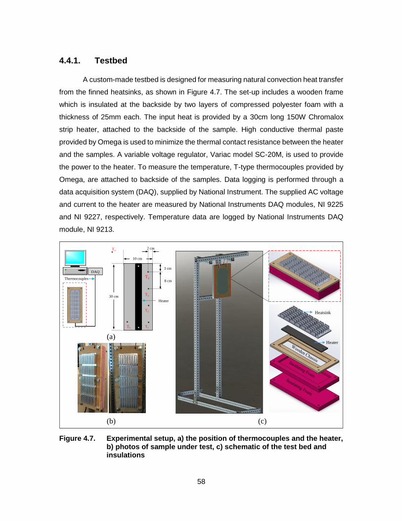
58
4.4.1. Testbed
A custom-made testbed is designed for measuring natural convection heat transfer
from the finned heatsinks, as shown in Figure 4.7. The set-up includes a wooden frame
which is insulated at the backside by two layers of compressed polyester foam with a
thickness of 25mm each. The input heat is provided by a 30cm long 150W Chromalox
strip heater, attached to the backside of the sample. High conductive thermal paste
provided by Omega is used to minimize the thermal contact resistance between the heater
and the samples. A variable voltage regulator, Variac model SC-20M, is used to provide
the power to the heater. To measure the temperature, T-type thermocouples provided by
Omega, are attached to backside of the samples. Data logging is performed through a
data acquisition system (DAQ), supplied by National Instrument. The supplied AC voltage
and current to the heater are measured by National Instruments DAQ modules, NI 9225
and NI 9227, respectively. Temperature data are logged by National Instruments DAQ
module, NI 9213.
Figure 4.7. Experimental setup, a) the position of thermocouples and the heater, b) photos of sample under test, c) schematic of the test bed and insulations
Heatsink
Heater
T1
T2
T3
T4
T5
T∞
10 cm
2 cm
30 cm
3 cm
8 cm
Heater
DAQ
Thermocouples
(a)
(b) (c)

59
Thirteen samples with the same fin height and baseplate dimensions are prepared.
To ensure similar surface finishing for all the samples, CNC machining was used to
prepare the samples. Geometrical dimensions of the samples are designed in a way to
enable parametric study on fin spacing, fin length, and gap length. Based on the
developed model, fin parameters are selected to cover the optimum range. Dimensions of
the test samples are given in Table 4.2.
Table 4.2. Dimensions of the interrupted fin samples used in the experiments
Schematic and Sample Photos Sample Name s [mm] l [mm] G [mm] m n
Int. 9-30-10 9 30 10 7 9
Int. 9-10-10 9 10 10 15 9
Int. 9-20-10 9 20 10 10 9
Int. 9-40-10 9 40 10 6 9
Int. 9-50-10 9 50 10 5 9
Int. 9-140-10 9 140 10 2 9
Int. 5-30-10 5 30 10 7 13
Int. 7-30-10 7 30 10 7 10
Int. 11-30-10 11 30 10 7 8
Int. 13-30-10 13 30 10 7 7
Int. 9-30-6 9 30 6 1 9
Int. 9-30-8 9 30 8 8 9
Int. 9-300-0 9 300 0 8 9
4.4.2. Test Procedure
The experiments are performed in a windowless room with an environment free of
air currents. The room dimensions are selected to be large enough to ensure constant
ambient temperature during the test. The input power supplied to the heaters is monitored
and surface temperatures were measured at five locations at the back of the baseplate.

60
Four self-adhesive, copper-constantan thermocouples (Omega, T-type) are attached in
vertical locations on one side of the samples backplate, as shown in Figure 4.7.a. An extra
thermocouple is installed on the same level with the lowest thermocouples, at the other
side of backplate, to make sure that the temperature is well distributed horizontally (T5 in
Figure 4.7.a). All thermocouples are taped down to the backside of the samples to prevent
disturbing the air flow on the finned side of the samples. An additional thermocouple is
used to measure the ambient temperature during the experiments. Temperature
measurements are performed at five points and the average value is taken as the
baseplate temperature. Among all the experiments, the maximum standard deviation from
the average temperature is measured to be less than 2.5˚C. Since the experiments are
performed to mimic the uniform wall temperature boundary condition, the thickness of the
baseplate and the fins are selected fairly high, 5mm and 3mm, respectively, to ensure the
minimum thermal bulk resistance and uniform temperature distribution in the samples. An
infrared camera, model SC655 from FLIR, is used to observe the temperature variation
along the fins. The maximum temperature difference between the fins and the baseplate
is measured to be about 2.1˚C, so the fins are assumed to be at the same temperature
with the baseplate. For each of the 13 samples, the experimental procedure is repeated
for different power inputs. Table 4.3 lists the range of some important test parameters.
The steady-state condition is considered to be achieved when the rate of all temperature
variations are less than 0.1˚C/hr which in average, takes 120 minutes for the test samples
used in the experiments.
Table 4.3. Range of some important parameters in test procedure
Parameter Description Range Unit
P Heater power 5-50 [W]
T Ambient temperature 24-27 [ᵒC]
wT Wall temperature 30-70 [ᵒC]
For the data analysis, heat transfer due to natural convection from the baseplate
and fin tips are calculated using the available correlations in literature [19], and subtracted
from total heat input to the system. Following Rao et al. [61], the effect of radiation heat
transfer is also subtracted from the fins total heat transfer (see Appendix B). Due to
relatively low surface temperature and low emissivity of machined aluminum (between

61
0.09 and 0.1), the effect of radiation is not significant. The maximum calculated value for
radiation heat transfer is 3.2% of total heat transfer.
4.4.3. Uncertainty Analysis
Uncertainty analysis for the experimental study of the interrupted fin heatsinks is
very similar to that performed in Section 2.2.3. Equations 2.6 to 2.10 are directly used for
the uncertainty analysis of the experimental study. Table 2.4 is also valid to be used for
the current experiments. Performing the uncertainty analysis for total heat transfer, the
maximum uncertainty value for . .N CQ is calculated to be 8%. The measured temperatures
uncertainty T is 2 ,C which is twice the accuracy of the thermocouples. The calculated
uncertainties for . .N CQ are reported as error bars in the experimental results.
4.4.4. Test Results
The comparison between the experimental data and the values obtained from the
combination of the channel solution and gap solution are shown in Figure 4.8 for different
values of ,T which is the difference between average surface temperature and ambient
temperature. The details on how to calculate the total heat transfer to develop the
analytical results of Figure 4.8 are explained in Section 4.5.1. As can be seen in the figure,
there is a fairly good agreement between the experimental data and the analytical solution.
For the fin spacing, ,s the maximum, minimum, and average relative difference between
the experimental data and closed-form solution is 32%, 2% and 10%, respectively (Figure
4.8.a). These values for the fin length, ,l are 26%, 1% and 11%, respectively (Figure 4.8.b).
Comparing the result from analytical solution to the experimental data, gives maximum,
minimum, and average relative difference of 23%, 1% and 7%, respectively for the gap
length,G (Figure 4.8.c). Maximum errors always occur at low temperature differences
between the surface and ambient, 7 ,T C which is not normally a value for naturally-
cooled heatsinks in real applications.

62
Figure 4.8. Comparison between the experimental data and analytical solution, a) fin spacing, b) fin length, c) gap length
0
10
20
30
40
50
60
0.004 0.006 0.008 0.01 0.012 0.014
Q[W
]
s [m]
ΔT=7ᵒC
(a)
0
10
20
30
40
50
60
0 0.05 0.1 0.15 0.2 0.25 0.3
Q[W
]
l [m]
ΔT=7ᵒC
(b)
0
10
20
30
40
50
60
70
80
0.005 0.006 0.007 0.008 0.009 0.01 0.011 0.012
Q[W
]
G [m]
ΔT=12ᵒC
ΔT=7ᵒC
(c)

63
4.4.5. Validity of Uniform Wall Temperature Assumption
One of the major assumptions to develop our analytical model in section 4.2 is
uniform wall temperature as thermal boundary condition. In this section is we try to
examine the validity of this assumption by taking two different approaches: i) lumped
system analysis, ii) IR thermography.
A simple, yet reliable method to test the validity of uniform wall temperature
assumption is using Biot number as a measure for validity of “lumped system assumption”
[72]. Biot number, ,Bi hL k is ratio of convection to conduction heat transfer. The length
scale selected for this analysis is the baseplate length, ,L and h and k are convection heat
transfer coefficient and thermal conductivity of the aluminum heatsinks respectively. For
Biot numbers less than unity, thermal conductivity of the solid is larger than the convective
heat transfer coefficient at the solid-fluid interface. This implies that due to high resistance
against heat transfer at the solid boundaries, the heat generated at the source, can spread
through the solid and create more uniform temperature distribution. For the experimental
studies conducted in this section, the convective heat transfer coefficient is around 20
W/m2K, the baseplate length is 0.3 m, and the thermal conductivity of aluminum is around
200 W/mK. The Biot number for this conditions will be 0.03, which is much less than 0.1
and makes the lumped capacitance assumption valid.
To back up this analysis, infrared thermography is used to map the temperature of
the heatsinks under test condition. Figure 4.9 shows a sample of IR images. Two series
of IR images are taken, one from front and the other from side of the heatsinks. Figure
4.9.a shows the temperature distribution in the heatsink sample, to verify the uniform
heatsink temperature assumption. As shown in this Figure 4.9, the maximum, minimum
and average temperature of the heatsink is 51˚C, 48˚C, and 49˚C respectively. The IR
image in Figure 4.9.b shows the temperature distribution along the fins, to verify the
uniform wall temperature assumption. As shown, the maximum, minimum and average
temperature of a single fin is measured 50˚C, 48˚C, and 49˚C respectively, which makes
the uniform wall temperature, a fair assumption.

64
Figure 4.9. IR image from a) front view, b) side view of the heatsink sample under test
4.5. Results and Discussion
4.5.1. Total Heat Transfer Calculation
Having all the geometrical parameters, fin height, ,H fin thickness, ,t fin spacing, ,s
fin length, ,l and gap length, ,G known, on a baseplate with dimensions L and ,W number of
fin rows, ,m and number of fin columns, ,n can be calculated as follows;
L
ml G
4.31
Tmax= 323.9 K
Tmin= 320.2 K
Tavg= 321.8 K
Tmax= 323.2 K
Tmin= 321.7 K
Tavg= 322.1 K
(a) (b)

65
W
ns t
4.32
The total heat transfer area can be calculated as follows;
2A m nl H 4.33
To calculate the heat flux from the first row of fins, Eq. 4.3 for the inlet velocity to
the first row, , ,1 ,C inu can be substituted into Eq. 4.4 to find the heat transfer coefficient
associated with first row of fins, 1.h The calculated heat transfer coefficient can be
substituted in Eq. 4.34 to find the heat flux, knowing that the inlet temperature to the first
row, C,in,1 ,T is equal to ambient temperature, .T
1 1 , ,1( )w C inq h T T 4.34
Now Eqs. 4.21 and 4.22 can be used to find the inlet condition to the first gap , ,1G inu
and , ,1G inT . Having the first gap inlet conditions, Eqs. 4.23 and 4.24 can be used to calculate
the average inlet velocity , ,2C inu and temperature , ,2C inT to the second row of fins. The
same procedure can be followed to find the heat flux for the thi row of fins, until the march
through all the rows is finished. The total heat flux and total heat transfer can be found as
follows;
1
m
i
i
q q
4.35
Q Aq 4.36
All fluid properties can be evaluated at the average temperature, / 2.avg wT T T
A simple computer code, in any language, can be developed to find the heat flux and total
heat transfer from any arbitrary fin arrangement.
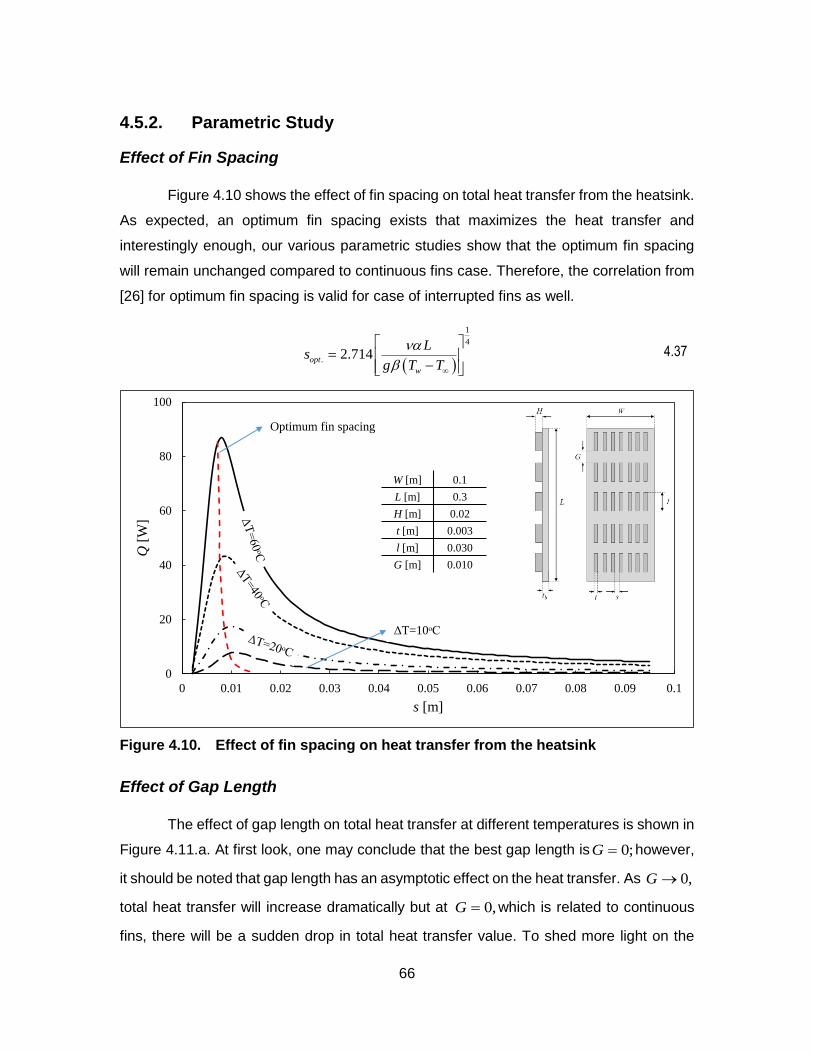
66
4.5.2. Parametric Study
Effect of Fin Spacing
Figure 4.10 shows the effect of fin spacing on total heat transfer from the heatsink.
As expected, an optimum fin spacing exists that maximizes the heat transfer and
interestingly enough, our various parametric studies show that the optimum fin spacing
will remain unchanged compared to continuous fins case. Therefore, the correlation from
[26] for optimum fin spacing is valid for case of interrupted fins as well.
1
4
. 2.714opt
w
Ls
g T T
4.37
Figure 4.10. Effect of fin spacing on heat transfer from the heatsink
Effect of Gap Length
The effect of gap length on total heat transfer at different temperatures is shown in
Figure 4.11.a. At first look, one may conclude that the best gap length is 0;G however,
it should be noted that gap length has an asymptotic effect on the heat transfer. As 0,G
total heat transfer will increase dramatically but at 0,G which is related to continuous
fins, there will be a sudden drop in total heat transfer value. To shed more light on the
0
20
40
60
80
100
0 0.01 0.02 0.03 0.04 0.05 0.06 0.07 0.08 0.09 0.1
Q[W
]
s [m]
ΔT=10ᵒC
Optimum fin spacing
W [m] 0.1
L [m] 0.3
H [m] 0.02
t [m] 0.003
l [m] 0.030
G [m] 0.010

67
effect of gap length, Figure 4.11.b shows the ratio of heat transfer from interrupted fins to
the heat transfer from continuous fins with the same fin spacing, ./ ,contQ Q versus / .G L This
figure shows how at small values of gap length the heat transfer from interrupted fins
dominate the heat transfer from continuous fins, due to the effect of gap on thermal
boundary layer. As the gap length increases, due to loss of heat transfer area, total heat
transfer keeps decreasing until the interrupted fin arrangement loses its privilege over
continuous fins. It is also worth mentioning that as gap length increases, the weight of
heatsink decreases, which can play a key role for the applications in which weight is an
important matter.
Effect of Fin Length
Figure 4.12.a shows the total heat transfer from the fins for different fin lengths at
various surface temperatures. As shown in the figure, fin length plays an important role in
the heatsink performance. Depending on the baseplate dimensions, an optimum fin length
can be found to maximize the total heat transfer rate. Figure 4.12.b shows the ratio of heat
transfer from interrupted fins to continuous fins, which as shown, can be over 12 times
more for the specific case shown in Figure 4.12.b.
A noteworthy trend that can be observed in Figure 4.12.b is that the enhancement
effect of adding interruptions to the fins decreases at higher temperatures. The reason for
this phenomena is that the buoyancy force is stronger at higher temperatures, causing
more air flow to pass from the channel. More air flow leads to higher velocity and heat
transfer rate. Adding interruption to fins at high surface temperatures, decreases this effect
by removing high temperature solid surface, which is the main cause for buoyancy force.
However at practical ranges of heatsink temperature, 40 60 ,C interrupted fin
arrangement can dissipate heat about 3 times more than continuous fins, which is still a
considerable contribution to the heatsink performance.

68
Figure 4.11. Effect of gap length on heat transfer from the heatsink, a) total heat transfer, b) dimensionless heat transfer with respect to continuous fins
0
20
40
60
80
100
120
140
160
180
0 0.05 0.1 0.15 0.2 0.25 0.3
Q[W
]
G [m]
ΔT=10ᵒC
W [m] 0.1
L [m] 0.3
H [m] 0.02
t [m] 0.003
s [m] 0.009
l [m] 0.003
(a)
0
1
2
3
4
5
6
0.0 0.1 0.2 0.3 0.4 0.5 0.6 0.7 0.8 0.9
Q/Q
con
t.
G/L
ΔT=10ᵒC to 60ᵒC
(b)

69
Figure 4.12. Effect of fin length on heat transfer from the heatsink, a) total heat transfer, b) dimensionless heat transfer with respect to continuous fins
0
10
20
30
40
50
60
70
80
90
0 0.05 0.1 0.15 0.2 0.25 0.3
Q[W
]
l [m]
W [m] 0.1
L [m] 0.3
H [m] 0.02
t [m] 0.003
s [m] 0.009
G [m] 0.010
(a)
0
2
4
6
8
10
12
14
0.0 0.1 0.2 0.3 0.4 0.5 0.6 0.7 0.8 0.9 1.0
Q/Q
con
t.
l/L(b)
ΔT=40ᵒC
ΔT=60ᵒC

70
4.5.3. Heatsink Design Procedure
In this section, it is intended to find the best fin arrangement, by determining the
geometrical parameters, to maximize the total heat transfer rate from an available surface
area, with a known operating temperature. The design procedure for the fin arrangement
is explained in this section as following;
Step 1: Selecting the fin thickness, .t Fin thickness selection is mostly a matter of
mechanical strength, so depending on the application and required robustness of the
heatsink, the fin thickness can be selected. However, when selecting the thickness of the
fins, we should keep in mind that thicker fins present lower thermal bulk resistance, which
leads to more uniform temperature distribution along the fin and higher heat transfer. It
also worth noting that thicker fin means heavier heatsink.
Step 2: Calculating the optimum fin spacing, .,opts using Eq. 4.37. The number of fin
columns can be evaluated using Eq. 4.32, when the optimum fin spacing is determined.
Step 3: Determining the gap length, .G Selecting the gap length is highly dependent
on manufacturing limitations, cost, and weight considerations. As shown in Section 4.5.2,
the smaller gap length leads to higher total heat transfer rate; however sometimes due to
manufacturing limitations, small gap length is not practical. Very small gaps can also get
blocked due to contamination and corrosion and lose their effects. On the other hand, the
higher the gap, the lighter the heatsink. Therefore, in applications where weight is a limiting
factor, higher gap lengths are better choices. Based on the above-mentioned
considerations, one or more gap length option(s) can be selected for the analysis in next
step.
Step 4: Finding the optimum fin length. Having all the fin parameters determined,
and assuming an average operation temperature for the heatsink, a simple computer code
can be used to perform a parametric study on the fin length to maximize the total heat
transfer from the heatsink.
71
4.6. Conclusion
A new analytical solution for steady-state laminar natural convection from
isothermal vertical rectangular interrupted fins is presented and close-form compact
correlations are introduced for velocity and temperature distribution for the first time.
Integral technique was used in combination with numerical simulations to solve the
governing equation. A custom-made testbed is built and 13 different aluminum heatsinks
are tested to validate the numerical and analytical results. An easy-to-apply method is
introduced, using the obtained correlations, to calculate total heat transfer from any
arbitrary arrangement of interrupted fins, and a step-by-step method is presented to
design naturally-cooled heatsinks with interrupted fins. Results show that naturally-cooled
heatsinks with interrupted fins are capable of dissipating heat up to 12 time higher than
currently available heatsinks with similar baseplate dimensions. This is while the weight
of such heatsinks can get up to 30% lighter than the heatsinks with continuous fins, but
similar baseplate dimensions.

72
Chapter 5. Summary and Future Work
5.1. Summary of Thesis
Advantages such as; being noise-free, reliable with no parasitic power demand,
and less maintenance requirements, make passive cooling a preferred thermal
management solution for electronics. The focus of this thesis is to design high
performance naturally-cooled heatsinks, to increase the cooling capacity of available
passive thermal management systems. Heatsinks with interrupted rectangular vertical fins
are the target of this study.
Due to the complexities associated with interrupted fins, interrupted rectangular
single wall is chosen as the starting point of the project. Asymptotic solution and blending
technique is used to present a compact correlation for average Nusselt number of such
wall, for the first time. The proposed correlation is verified by the results obtained from
numerical simulations, and experimental data obtained from a custom-designed testbed.
In the next step natural convection heat transfer from parallel plates is considered.
Integral technique is used to solve the governing equations, and closed-form correlations
for velocity, temperature, and local Nusselt number are developed for the first time. The
results are successfully verified with the result of an independent numerical simulation and
experimental data obtained from tests conducted on aluminum heatsink sample.
In the last step, to model heat transfer from interrupted finned heatsinks, analytical
approach is used, to obtain compact correlations for velocity and temperature inside the
domain. Numerical simulations are performed to provide some information, required by
our analytical approach. An extensive experimental study is also conducted to verify the
results from analytical solution and numerical simulation. Results show that the new-
designed heatsinks are capable of dissipating heat up to 12 times more than currently
available naturally-cooled heatsinks, with weight up to 30% lighter. The new heatsinks can

73
increase the capacity of passive cooling systems significantly. The list of contributions
resulted from the present study is listed below;
• Developing a closed-form correlation for average Nusselt number from interrupted single walls [73]
• Introducing an effective length to describe heat transfer from interrupted single walls analogous to heat transfer from a continuous vertical wall [73]
• Developing closed-form solutions for local Nusselt number, velocity, and temperature distribution in laminar natural convection heat transfer between parallel plates [74]
• Developing compact correlation for velocity and temperature in two dimensional momentum and energy diffusion in a one directional laminar flow, submitted to international journal of heat and mass transfer
• Design of interrupted fin naturally-cooled heatsinks with average heat dissipation of 5 time higher than similar commercially available heatsinks [55]
• Developing an easy to use tool to design high performance naturally-cooled heatsinks with interrupted fins, submitted to international journal of heat and mass transfer
• Design and prototyping of a fully passive thermal management system for outside plant telecom enclosures [15]
5.2. Future Work
The following research directions can be considered as the continuation of this
dissertation:
• Extend the analysis to other fin orientations, such as inclined fins or louvered fins (see Figure 5.1.a). Inclined fins have the potential to accommodate higher fin density on an available surface area, and also to create separate paths for fresh air and hot air.
• Extend the analysis to fin arrangement with variable fin/gap length along the flow (see Figure 5.1.b). Considering the significant effect of geometrical parameters on heat transfer, variation of these parameters in a way that they can adopt to the flow characteristic could be a potential improvement to this work.
• Extend the analysis to conductive heat transfer inside the heatsink and fins, to include the effect of bulk and spreading resistance in the problem. Numerical methods can be the best option to solve this problem.
• Investigate the effects of thermal load variations, i.e. transient natural convection heat transfer from interrupted fins, however; due to high thermal

74
inertia in naturally-cooled systems quasi-steady models may be sufficient to predict the system behavior.
• To investigate the effect of surface roughness on natural convection heat transfer from the heatsinks.
Figure 5.1. Proposed geometries for the future work, a) inclined interrupted fins, b) variable fin parameters along the flow
Co
ld a
ir
Ho
t ai
r
Co
ld a
ir
(a) (b)
75
References
[1] Anandan S., and Ramalingam V., 2008, “Thermal management of electronics: A review of literature,” Int. J. Therm. Sci., 12(2), pp. 5–26.
[2] Gurrum S. P. S., Suman S., Shivesh K., Joshi Y. K., and Fedorov A. G., 2004, “Thermal Issues in Next-Generation Integrated Circuits,” IEEE Trans. DEVICE Mater. Reliab., 4(4), pp. 709–714.
[3] Wankhede M., Khaire V., and Goswami A., 2007, “evaluation of cooling solutions for outdoor electronics,” 13th International Conference on Thermal Investigation of ICs and Systems, ©EDA Publishing, Budapest, Hungary, pp. 1–6.
[4] Jahkonen J., Puolakka M., and Halonen L., 2013, “Thermal Management of Outdoor LED Lighting Systems and Streetlights Variation of Ambient Cooling Conditions,” LEUKOS, 9(3), pp. 155–176.
[5] Christensen A., Ha M., and Graham S., 2007, “Thermal Management Methods for Compact High Power LED Arrays,” 7th International Conference on Solid State Lighting, I.T. Ferguson, N. Narendran, T. Taguchi, and I.E. Ashdown, eds., SPIE UK, San Diego, California, USA, p. 66690Z–66690Z–19.
[6] BCCResearch, 2014, The Market for Thermal Management Technologies, Wellesley, MA, USA.
[7] 2012, Information and Communication Technology Portfolio: Improving Energy Efficiency and Productivity in America’s Telecommunication Systems and Data Centers.
[8] Roy S. N., 2008, “Energy logic: A road map to reducing energy consumption in telecommunications networks,” INTELEC 2008 - 2008 IEEE 30th Int. Telecommun. Energy Conf., pp. 1–9.
[9] Lange C., Kosiankowski D., Weidmann R., and Gladisch A., 2011, “Energy Consumption of Telecommunication Networks and Related Improvement Options,” IEEE J. Sel. Top. Quantum Electron., 17(2), pp. 285–295.
[10] Lange C., Kosiankowski D., Gerlach C., Westphal F., and Gladisch A., 2009, “Energy Consumption of Telecommunication Networks,” 35th European Conference on Optical Communication, ECOC 09, IEEE, Vienna, pp. 1–2.
[11] Kilper D. C., Member S., Atkinson G., Korotky S. K., Goyal S., Vetter P., Suvakovic D., and Blume O., 2011, “Power Trends in Communication Networks,” Sel. Top. Quantum Electron., 17(2), pp. 275–284.

76
[12] Lubritto C., and Petraglia A., 2008, “Telecommunication power systems: energy saving, renewable sources and environmental monitoring,” IEEE Electrical Power & Energy Conference (EPEC), Vancouver Canada, pp. 1–4.
[13] Hernon D., Silvestre-Castillo P., and Hayden P., 2011, “Significantly extending the operational range of free cooling in radio Base Station indoor shelters,” IEEE 33rd International Telecommunications Energy Conference (INTELEC), Ieee, Amsterdam, Netherlands, pp. 1–7.
[14] Gholami A., 2014, “A New Integrated Approach for Modeling Green Passive Cooling Systems,” M.A.Sc. Thesis, Simon Fraser University.
[15] Ahmadi M., Gholami A., Lau K., and Bahrami M., 2014, “Passive Cooling of Outside Plant Power Systems , a Green Solution to Reduce Energy Consumption,” IEEE 36th International Communications Energy Conference (INTELEC), IEEE, Vancouver Canada, pp. 1–9.
[16] Ostrach S., 1952, "An analysis of laminar free-convection flow and heat transfer about a flat plate parallel to the direction of the generating body force," Thecnical Report, NACA.
[17] Sparrow E., and Gregg J., 1956, “Laminar free convection from a vertical plate with uniform surface heat flux,” ASME J. Heat Transf., 78(1), pp. 435–440.
[18] Merkin J., 1985, “A note on the similarity solutions for free convection on a vertical plate,” J. Eng. Math., 19(1), pp. 189–201.
[19] Churchill S. W., and Chu H., 1975, “Correlating equations for laminar and turbulent free convection from a vertical plate,” Int. J. Heat Mass Transf., 18(11), pp. 1323–1329.
[20] Yovanovich M., and Jafarpur K., 1993, “Bounds on Laminar Natural Convection From Isothermal Disks and Finite Plates of Arbitrary Shape for All Orientations and Prandtl Numbers,” ASME Winter Annual Meeting, New Orleans, Louisiana, pp. 93–111.
[21] Cai R., and Zhang N., 2003, “Explicit analytical solutions of 2-D laminar natural convection,” Int. J. Heat Mass Transf., 46(5), pp. 931–934.
[22] Yousefi T., and Ashjaee M., 2007, “Experimental study of natural convection heat transfer from vertical array of isothermal horizontal elliptic cylinders,” Exp. Therm. Fluid Sci., 32(1), pp. 240–248.
[23] Suryawanshi S., and Sane N., 2009, “Natural Convection Heat Transfer From Horizontal Rectangular Inverted Notched Fin Arrays,” J. Heat Transfer, 131(8), pp. 797–805.

77
[24] Elenbaas W., 1942, “Heat dissipation of parallel plates by free convection,” Physica, 9(1), pp. 1–28.
[25] Stuart W. Churchill, 1977, “A Comprehensive Correlation Equation for Buoyancy Induced Flow in Channels,” Lett. Heat Mass Transf., 4(3), pp. 193–199.
[26] Bar-Cohen A., and Rohsenow W. M., 1984, “Thermally Optimum Spacing of Vertical, Natural Convection Cooled, Parallel Plates,” J. Heat Transfer, 106(1), pp. 116–123.
[27] Bodoia J. R., and Osterle J. F., 1962, “The Development of Free Convection Between Heated Vertical Plates,” J. Heat Transfer, 84(1), pp. 40–44.
[28] Ofi O., and Hetherington H. J., 1977, “Application of the finite element method to natural convection heat transfer from the open vertical channel,” Int. J. Heat Mass Transf., 20(11), pp. 1195–1204.
[29] Culham J. R., Yovanovich M. M., and Lee S., 1995, “Thermal modeling of isothermal cuboids and rectangular heat sinks cooled by natural convection,” IEEE Trans. Components, Packag. Manuf. Technol. Part A, 18(3), pp. 559–566.
[30] Sparrow E. M., and Acharya S., 1981, “A natural convection fin with a solution-determined nonmonotonically varying heat transfer coefficient,” J. Heat Transfer, 103(2), pp. 218–226.
[31] Starner K. E., and McManus H. N., 1963, “An Experimental Investigation of Free-Convection Heat Transfer From Rectangular-Fin Arrays,” J. Heat Transfer, 85(3), pp. 273–275.
[32] Welling J. R., and Wooldridge C. B., 1965, “Free Convection Heat Transfer Coefficients From Rectangular Vertical Fins,” J. Heat Transfer, 87(4), p. 439.
[33] Edwards J., and Chaddock J., 1963, “An experimental investigation of the radiation and free convection heat transfer from a cylindrical disk extended surface,” ASHRAE Trans., 69(1), pp. 313–322.
[34] Chaddock J., 1970, “Natural Convection Heat Transfer from Vertical Rectangular Fin Array,” ASHRAE J, 12(August), pp. 53–60.
[35] Aihara T., 1970, “Natural Convection Heat Transfer from Vertical Rectangular Fin Arrays: (Part 3, Heat Transfer from Fin Flats),” Trans. Japan Soc. Mech. Eng., 13(64), pp. 1192–1200.
[36] Aihara T., 1970, “Natural Convection Heat Transfer from Vertical Rectangular Fin Arrays: (Part 2, Heat Transfer from Fin Edges),” Trans. Japan Soc. Mech. Eng., 36(282), pp. 239–247.

78
[37] Aihara T., 1970, “Natural Convection Heat Transfer from Vertical Rectangular Fin Arrays : (Part 1,Heat Transfer from Base Plates),” Trans. Japan Soc. Mech. Eng., 36(261), pp. 915–926.
[38] Aihara T., 1970, “Natural Convection Heat Transfer from Vertical Rectangular-Fin Arrays : Part 4, Heat-Transfer Characteristics of Nonisothermal-Fin Arrays,” Trans. Japan Soc. Mech. Eng., 36(292), pp. 2077–2086.
[39] Leung C. W., and Probert S. D., 1985, “Heat Exchanger: Optimal Separation for Vertical Ractangular Fins Proturding from Vertical Rectangular Base,” Appl. Energy, 19(1), pp. 77–85.
[40] Leung C. W., Probert S. D., and Shilston M. J., 1985, “Heat exchanger design: Optimal uniform separation between rectangular fins protruding from a vertical rectangular base,” Appl. Energy, 19(4), pp. 287–299.
[41] Leung C., Probert S., and Shilston M., 1985, “Heat exchanger design: thermal performances of rectangular fins protruding from vertical or horizontal rectangular bases,” Appl. Energy, 20(2), pp. 123–140.
[42] Leung C., Probert S., and Shilston M., 1986, “Heat transfer performances of vertical rectangular fins protruding from rectangular bases: effect of fin length,” Appl. Energy, 22(4), pp. 313–318.
[43] Leung C. W., and Probert S. D., 1987, “Natural-Convective Heat Exchanger with Vertical Rectangular Fins and Base: Design Criteria,” Proc. Inst. Mech. Eng. Part C J. Mech. Eng. Sci., 201(5), pp. 365–372.
[44] Leung C. W., and Probert S. D., 1989, “Heat-exchanger performance: Effect of orientation,” Appl. Energy, 33(4), pp. 235–252.
[45] Leung C. W., and Probert S. D., 1989, “Thermal effectiveness of short-protrusion rectangular heat exchanger fins,” J. Appl. energy, 34(1), pp. 1–8.
[46] Pol D. Van de, and Tierney J., 1974, “Free convection heat transfer from vertical fin-arrays,” IEEE Parts, Hybrids, Packag., 10(4), pp. 267–271.
[47] Dejong N. C., and Jacobi A. M., 1995, "An Experimental Study of Flow and Heat Transfer in Offset Strip and Louvered-Fin Heat Exchangers," Technical Report, ACRC, University of Illinois, Urbana.
[48] Brutz J. M., Dutton J. C., and Jacobi A. M., 2005, "Use of Unsteady Forcing in Interrupted-Fin Heat Exchangers: An Assessment of Potential," Technical Report, ACRC, University of Illinois, Urbana.

79
[49] Ndao S., Peles Y., and Jensen M. K., 2009, “Multi-objective thermal design optimization and comparative analysis of electronics cooling technologies,” Int. J. Heat Mass Transf., 52(19-20), pp. 4317–4326.
[50] Da Silva a. K. K., Lorente S., and Bejan a., 2004, “Optimal distribution of discrete heat sources on a wall with natural convection,” Int. J. Heat Mass Transf., 47(2), pp. 203–214.
[51] Sobel N., Landis F., and Mueller W., 1966, “NATURAL CONVECTION HEAT TRANSFER IN SHORT VERTICAL CHANNELS INCLUDING EFFECTS OF STAGGER,” Proc. 3rd Int. Heat Transf. Conf., 2(1), pp. 121–125.
[52] Sparrow E. M., and Prakash C., 1980, “Enhancement of Natural Convection Heat Transfer by a Staggered Array of Discrete Vertical Plates,” J. Heat Transfer, 102(2), pp. 215–220.
[53] Daloglu a., and Ayhan T., 1999, “Natural convection in a periodically finned vertical channel,” Int. Commun. Heat Mass Transf., 26(8), pp. 1175–1182.
[54] Gorobets V., 2002, “Heat transfer for vertical surfaces with discrete fins in the case of free convection,” J. Eng. Phys. Thermophys., 75(5), pp. 100–107.
[55] Ahmadi M., Mostafavi G., and Bahrami M., 2014, “Natural convection from rectangular interrupted fins,” Int. J. Therm. Sci., 82(1), pp. 62–71.
[56] Mostafavi G., 2012, “NATURAL CONVECTIVE HEAT TRANSFER FROM INTERRUPTED RECTANGULAR FINS,” M.A.Sc. Thesis, Simon Fraser University.
[57] Fujii M., 2007, “Enhancement of natural convection heat transfer from a vertical heated plate using inclined fins,” Heat Transf. Res., 36(6), pp. 334–344.
[58] Nada S. A., 2007, “Natural convection heat transfer in horizontal and vertical closed narrow enclosures with heated rectangular finned base plate,” Int. J. Heat Mass Transf., 50(3-4), pp. 667–679.
[59] Ben-Nakhi A., and Chamkha A. J., 2007, “Conjugate natural convection in a square enclosure with inclined thin fin of arbitrary length,” Int. J. Therm. Sci., 46(5), pp. 467–478.
[60] Bejan A., 2004, Convection heat transfer, John Wiley and Sons, Inc., New York.
[61] Rao V. D., Naidu S. V., Rao B. G., and Sharma K. V., 2006, “Heat transfer from a horizontal fin array by natural convection and radiation—A conjugate analysis,” Int. J. Heat Mass Transf., 49(19-20), pp. 3379–3391.
[62] Holman J. P., 2001, Experimental Methods for Engineers, McGrawHill, New York.

80
[63] McAdams W. H., 1954, Heat Transmission, McGrawHill, New York.
[64] Churchill S. W., and Usagi R., 1972, “A general expression for the correlation of rates of transfer and other phenomena,” AIChE J., 18(6), pp. 1121–1128.
[65] Güvenç A., and Yüncü H., 2001, “An experimental investigation on performance of fins on a horizontal base in free convection heat transfer,” J. Heat mass Transf., 37(1), pp. 409–416.
[66] Goldstein R. J., Sparrow E. M., and Jones D. C., 1973, “Natural convection mass transfer adjacent to horizontal plates,” Int. J. Heat Mass Transf., 16(5), pp. 1025–1035.
[67] Sparrow E. M. E., and Gregg J. L., 1958, “similar solutions for natural convection from a non isothermal vertical plate,” J. Heat Transfer, 80(1), pp. 379–386.
[68] Sparrow E. M., and Gregg J. L., 1956, “Laminar Free Convection Heat Transfer from the Outer Surface of a Vertical Circular Cylinder,” Trans. ASME, 78(1), pp. 1823–1829.
[69] Gebhart B., Pera L., and Schorr A. ., 1970, “Steady laminar natural convection plumes above a horizontal line heat source,” Int. J. Heat Mass Transf., 13(1), pp. 161–171.
[70] Jaluria Y., and Gebhart B., 1977, “Buoyancy-induced flow arising from a line thermal source on an adiabatic vertical surface,” Int. J. Heat Mass Transf., 20(2), pp. 153–157.
[71] Nat Vorayos, 2000, “Laminar natural convection within long vertical uniformly heated parallel-plate channels and circular tubes,” Oregon State University.
[72] Incropera F., DeWitt D., and Bergrnan T., 2007, Fundamentals of Heat and Mass Transfer (The 6th Edition).
[73] Ahmadi M., Mostafavi G., and Bahrami M., 2014, “Natural Convection From Interrupted Vertical Walls,” J. Heat Transfer, 136(11), pp. 112501/1–8.
[74] Ahmadi M., Fakoor-Pakdaman M., and Bahrami M., 2014, “Natural Convection from Vertical Parallel Plates: An Integral Method Solution,” J. Thermophys. Heat Transf., pp. 1–10.
[75] Saikhedkar N. H., and Sukhatme S. P., 1981, “Heat transfer from rectangular cross-sectioned vertical fin arrays,” Proceedings of the Sixth National Heat and Mass Transfer Conference, HMT, pp. 9–81.
[76] SPARROW E. M., and VEMURI S. B., “Natural convection/radiation heat transfer from highly populated pin fin arrays,” J. Heat Transfer, 107(1), pp. 190–197.

81
[77] Sparrow E. M., and Vemuri S. B., 1986, “Orientation effects on natural convection/radiation heat transfer from pin-fin arrays,” Int. J. Heat Mass Transf., 29(3), pp. 359–368.
[78] Azarkish H., Sarvari S. M. H., and Behzadmehr a., 2010, “Optimum geometry design of a longitudinal fin with volumetric heat generation under the influences of natural convection and radiation,” Energy Convers. Manag., 51(10), pp. 1938–1946.
[79] Holman J. P., 2010, Heat Transfer, McGrawHill, Boston.

82
Appendix A. Integral Method for Natural Convection
In this section, the integral method for natural convection heat transfer is explained. The goal of this section is to clarify the methodology to obtain the governing equations from the control volumes shown in Table 3.1. The problem here is explained for a general case, however extending the introduced equation here, to the governing equations of Table 3.1 is straight forward.
Consider a boundary layer flow driven by buoyancy forces originating from density variations in a fluid (Figure A1).
Figure A1. General control volume used in integral method for free convection
The integral conservation equations can be obtained by directly integrating the governing equations term-by-term across the control volume. Here, we start from first principles and perform mass, momentum, and energy balances on the integral control volume shown in the preceding figure.

83
Conservation of mass
Figure A2 shows the control volume considered for the mass conservation analysis.
Figure A2. Conservation of mass in a control volume
0
CVoutin mdt
dmm
0
udymx
dxmx
mm xxdxx
dxudydx
dmd
0

84
Conservation of momentum
Figure A3 shows the control volume considered for the momentum conservation analysis.
Figure A3. Conservation of momentum in a control volume. Note that w is per
unit depth in z-direction.
0
,,,
CVxoutxinxx Mdt
dMMF
forcebuoyancy 000
dxdygdypdyp xdxxx
Thus, the x-momentum balance becomes:
0
0
2
00
dx
dyu
Mx
MMdxdygdxdygdx xxxxxw
Using ( ),T T we obtain:
w
x
T
dyTTgdyudx
d
00
2
where the integration limits have been set, keeping in mind that outside the hydrodynamic boundary layer the velocity is zero, and the temperature outside the thermal boundary layer is ambient temperature. The shear stress at the wall can be defined as;
0
w
y
u
y

85
Conservation of energy
The dominant terms relevant to the energy balance are shown in Figure A4. Consistent with the usual boundary layer approximations, heat conduction in the x-direction is neglected.
Figure A4. Conservation of energy in a control volume. Note that "wq is per unit
depth in z-direction.
0
CVoutin Edt
dEE
000
dxTdyuc
dx
ddxudy
dx
dTcdxq
T
ppw
which can be rearranged to:
p
w
c
qudy
dx
dTdyTTu
dx
d T
0
,min
0
where the heat flux at the wall can be defined as;
0
"w
y
Tq k
y

86
Appendix B. Calculation of Radiation Heat Transfer from Test Samples
Depending on the application and range of temperature, radiation heat transfer can play an important role in the heat transfer from fin arrays. This has been shown by Edwards and Chaddock [33], Chaddock [34], Sparrow and Acharya [30], Saikhedkar and Sukhatme [75], Sparrow and Vemuri [76,77], Azarkish et al. [78], and Rao et al. [61]. The common conclusion of the aforementioned studies is that the radiation heat transfer contributes 25% to 40% to the total heat transfer from fin arrays in the naturally-cooled heatsinks. However; in case of our experimental studies we measured the contribution of the radiation heat transfer to be around 5% of total measured heat transfer. This difference is mainly caused by the difference between the surface emissivity of the test samples. In most of the above mentioned studies anodized sample are used in the testing procedure. Adonization can increase the emissivity of aluminum to approximately 0.9, [79] which has a significant effect on radiation heat transfer from aluminum heatsinks. Reported emissivity for machined aluminum is in the range of 0.1 [79]. In this section, the methodology to approximate radiation heat transfer from the heatsink samples is explained. Figure B1 shows the domain considered for radiation analysis of the heatsink samples.
Figure B1. a) top view of the geometry considered for radiation heat transfer analysis, b) surfaces and temperatures used in view factor analysis
To perform the analysis we assume the length of the heatsink normal to the page, ,L is
larger than fin height, H and fin spacing, .s The surrounding might be represented by
hypothetical surface 2.A The net rate of radiation heat transfer to this surface is therefore
equivalent to the rate of heat rejection by a unit section of the array.
4 4
.,2 1 12Rad wQ A F T T
H
s Tw
T∞
W
A1=(2H+s)L
T=Tw
A2=sL
T=T∞
(a) (b)
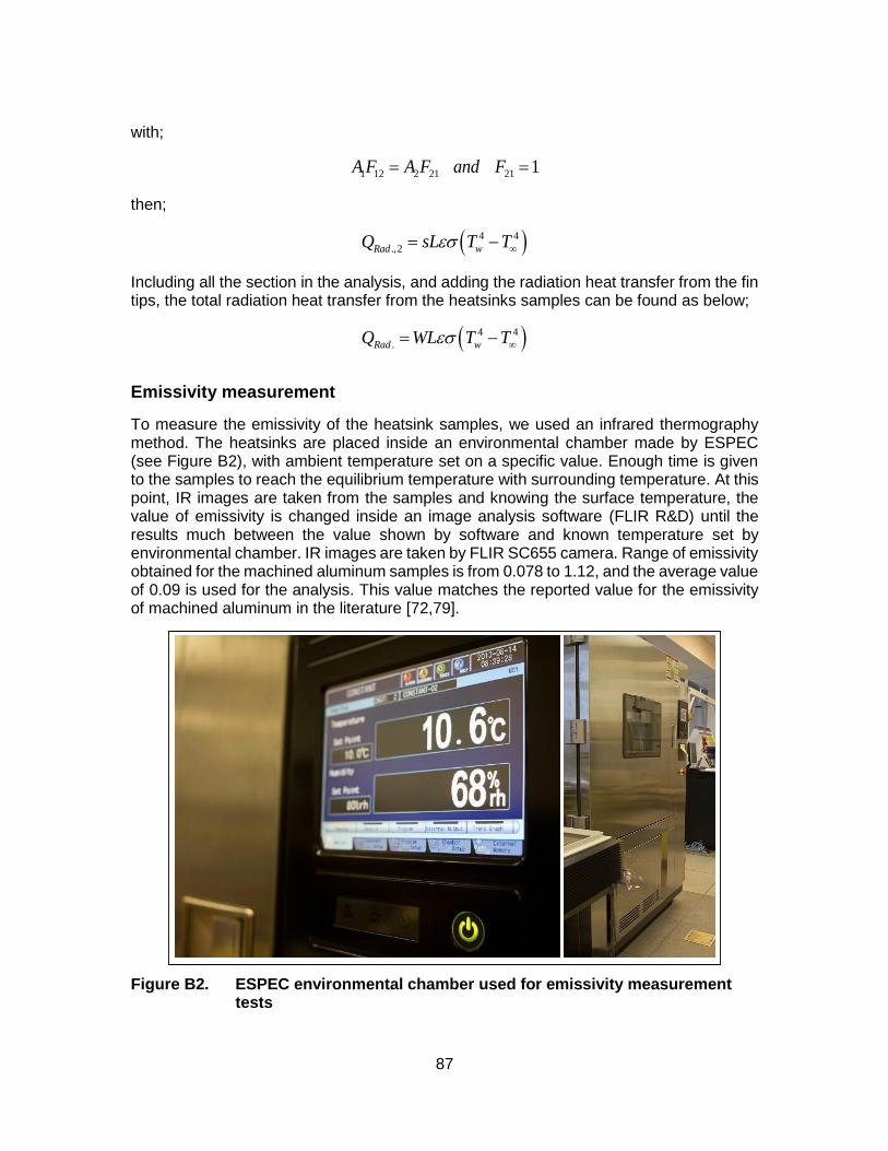
87
with;
1 12 2 21 21 1A F A F and F
then;
4 4
.,2Rad wQ sL T T
Including all the section in the analysis, and adding the radiation heat transfer from the fin tips, the total radiation heat transfer from the heatsinks samples can be found as below;
4 4
.Rad wQ WL T T
Emissivity measurement
To measure the emissivity of the heatsink samples, we used an infrared thermography method. The heatsinks are placed inside an environmental chamber made by ESPEC (see Figure B2), with ambient temperature set on a specific value. Enough time is given to the samples to reach the equilibrium temperature with surrounding temperature. At this point, IR images are taken from the samples and knowing the surface temperature, the value of emissivity is changed inside an image analysis software (FLIR R&D) until the results much between the value shown by software and known temperature set by environmental chamber. IR images are taken by FLIR SC655 camera. Range of emissivity obtained for the machined aluminum samples is from 0.078 to 1.12, and the average value of 0.09 is used for the analysis. This value matches the reported value for the emissivity of machined aluminum in the literature [72,79].
Figure B2. ESPEC environmental chamber used for emissivity measurement tests