putting table cartograms into practice

Putting Table Cartograms into Practice?

Mohammad Rakib Hasan, Debajyoti Mondal,Jarin Tasnim, and Kevin A. Schneider

Department of Computer ScienceUniversity of Saskatchewan, Saskatoon, Canada

{rakib.hasan,d.mondal,jarin.tasnim,kevin.schneider}@usask.ca

Abstract. Given an m× n table T of positive weights, and a rectangleR with an area equal to the sum of the weights, a table cartogram com-putes a partition of R into m × n convex quadrilateral faces such thateach face has the same adjacencies as its corresponding cell in T , and hasan area equal to the cell’s weight. In this paper, we examine constraintoptimization-based and physics-inspired cartographic transformation ap-proaches to produce cartograms for large tables with thousands of cells.We show that large table cartograms may provide diagrammatic rep-resentations in various real-life scenarios, e.g., for analyzing correlationsbetween geospatial variables and creating visual effects in images. Our ex-periments with real-life datasets provide insights into how one approachmay outperform the other in various application contexts.

Keywords: Cartography, Algorithms, Optimization, Image Processing

1 Introduction

A table cartogram is a cartographic representation for a two dimensional posi-tive matrix or tabular data. Given a positive m × n matrix of weights, a tablecartogram represents each cell as a distinct convex quadrilateral with an areaproportional to the corresponding cell’s weight such that the cell adjacencies arepreserved, the quadrilaterals form a partition of a rectangle R, and the sum ofall weights is equal to the area of R.

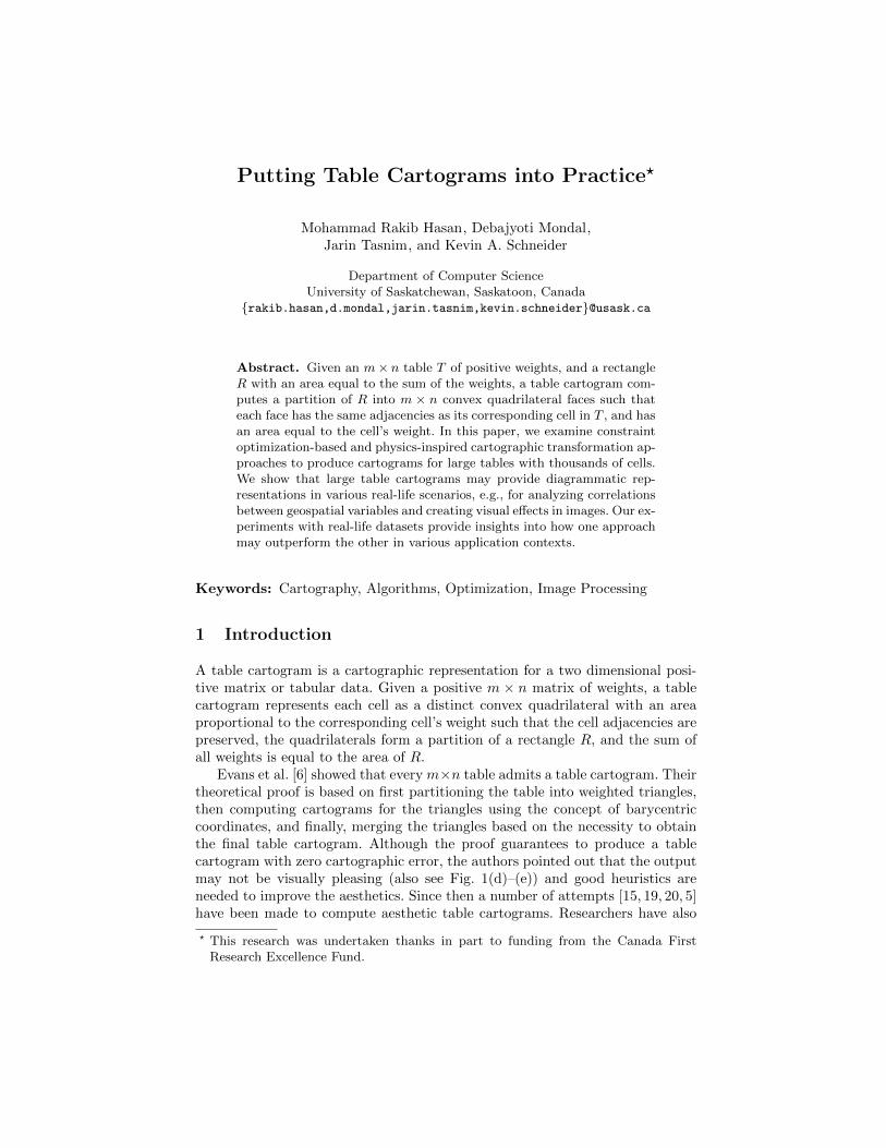
Evans et al. [6] showed that every m×n table admits a table cartogram. Theirtheoretical proof is based on first partitioning the table into weighted triangles,then computing cartograms for the triangles using the concept of barycentriccoordinates, and finally, merging the triangles based on the necessity to obtainthe final table cartogram. Although the proof guarantees to produce a tablecartogram with zero cartographic error, the authors pointed out that the outputmay not be visually pleasing (also see Fig. 1(d)–(e)) and good heuristics areneeded to improve the aesthetics. Since then a number of attempts [15, 19, 20, 5]have been made to compute aesthetic table cartograms. Researchers have also

? This research was undertaken thanks in part to funding from the Canada FirstResearch Excellence Fund.

2 Hasan et al.

Fig. 1: (a) A table T . (b) A table cartogram of T using constraint optimization.(c) Evans et al.’s [6] output for T (based on a theoretical proof). (d) A cartogramfor a large table based on constraint optimization, where (e) Evans et al.’s [6]approach produces skinny triangles.

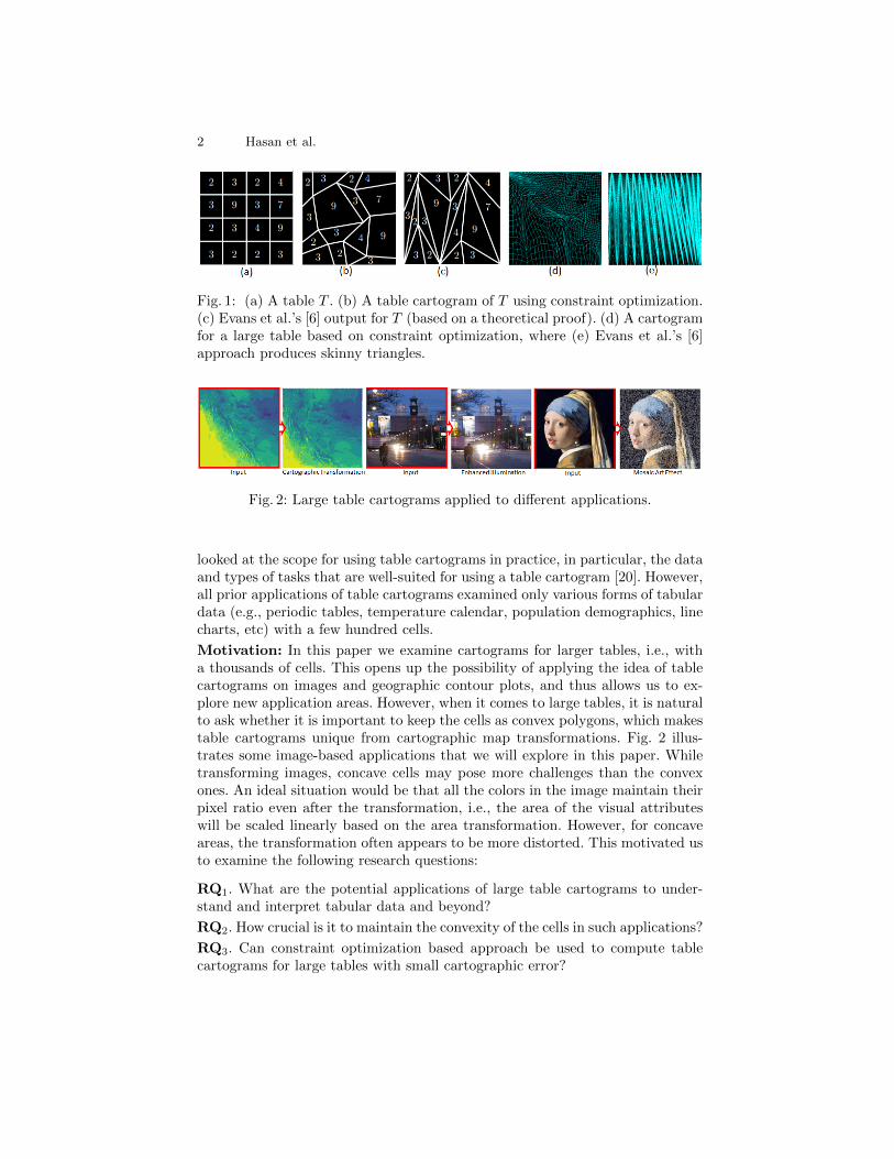
Fig. 2: Large table cartograms applied to different applications.

looked at the scope for using table cartograms in practice, in particular, the dataand types of tasks that are well-suited for using a table cartogram [20]. However,all prior applications of table cartograms examined only various forms of tabulardata (e.g., periodic tables, temperature calendar, population demographics, linecharts, etc) with a few hundred cells.

Motivation: In this paper we examine cartograms for larger tables, i.e., witha thousands of cells. This opens up the possibility of applying the idea of tablecartograms on images and geographic contour plots, and thus allows us to ex-plore new application areas. However, when it comes to large tables, it is naturalto ask whether it is important to keep the cells as convex polygons, which makestable cartograms unique from cartographic map transformations. Fig. 2 illus-trates some image-based applications that we will explore in this paper. Whiletransforming images, concave cells may pose more challenges than the convexones. An ideal situation would be that all the colors in the image maintain theirpixel ratio even after the transformation, i.e., the area of the visual attributeswill be scaled linearly based on the area transformation. However, for concaveareas, the transformation often appears to be more distorted. This motivated usto examine the following research questions:

RQ1. What are the potential applications of large table cartograms to under-stand and interpret tabular data and beyond?

RQ2. How crucial is it to maintain the convexity of the cells in such applications?

RQ3. Can constraint optimization based approach be used to compute tablecartograms for large tables with small cartographic error?

Putting Table Cartograms into Practice 3

RQ4. How constraint optimization based table cartogram compares to the carto-graphic map transformation algorithms in various quality metrics (e.g., numberof convex cells, aspect ratio, etc.)?

Contribution: In this paper we propose TCarto, a constraint based optimiza-tion approach that leverages parallel computing to deform a table via local op-timization using quadratic programming [13, 7]. TCarto can handle tables overhundred thousands of cells (e.g., 512× 512 tables in a few hours) and maintainsconvexity of each cell. We also adapt a physics-inspired cartographic transfor-mation approach — FastFlow [10], which may produce cartograms with concavecells.

We show that both TCarto and FastFlow (and thus large table cartograms)can potentially be useful in several real-life scenarios, e.g., for analyzing correla-tions between geospatial variables, and creating visual effects in images. We alsocompare the performances of TCarto and FastFlow empirically with two differ-ent real-life datasets: a meteorological dataset and a US State-to-State migrationflow dataset. In particular, we examine well-known metrics for measuring carto-graphic errors, number of concave cells and mean aspect ratio of the cells. Formeteorological dataset, where the data distribution does not contain high spikesand many local optima, both TCarto and FastFlow performed well, and Fast-Flow produced only a few concave cells. For the migration dataset with manysharp local optima, both TCarto and FastFlow produced low quality output,whereas for FastFlow we observed hundreds of concave cells. We also show howadding additional angle constraints can help mitigate this problem. The codeand data is available at GitHub1.

2 Related work

Cartographic representation of maps is a classic area of research. The surveysby Tobler [23] and by Nusrat and Kobourov [21] compiles historical progressin this area since the 1960s. Early algorithms were based on the metaphor thatconsiders the original map as a rubber sheet, and defines forces on the points suchthat they move to realize the cartographic representation. A major challenge insuch an approach is to ensure fast convergence, and preserve the shape of theregions on the map. Many algorithms [3, 4, 14] have been proposed to tacklethese challenges, yet the slow convergence remained a problem.

The diffusion-based algorithm [9] is another popular method for drawing con-tiguous cartograms. This is inspired by the idea of diffusion in physics, where thepoints move from high density to the low-density regions. A diffusion-based algo-rithm often produces blob and spike like artifacts, and narrow corridors. HenceCano et al. [2] proposed mosaic cartograms, where regions are represented asa set of regular tiles of the same size. The tiles help compare the regions viacounting, better preserve the shape, but also have a cost of making windingregion boundaries and tentacles like artifacts. There exist many approaches be-yond rubber sheet or diffusion based algorithms. For example, medial-axis based

1 https://github.com/rakib045/tcarto applications

4 Hasan et al.

cartogram [18] that transforms the regions based on the medial axis of the mappolygon, neural network based approach inspired by self-organizing map [12],etc.

In 2013, Sun [22] presented a rubber-sheet inspired algorithm (Carto3F) thatsignificantly improves the computational efficiency by using a quadtree struc-ture, and eliminates the topological error by adding appropriate conditions whilecomputing forces. In addition, the implementation of Carto3F exploits paral-lel computation. Recently, Gastner et al. [10] proposed a flow-based technique(FastFlow), inspired by the way particles of varying density into the water dif-fuse across the water over time that also leverages parallelism for fast cartogramcomputation.

Table cartograms [6] were proposed to visualize tabular data, where cellsare restricted to be convex and to form a tiling of a rectangle. However, if werelax table cartogram constraints, then it is possible to use existing physics-inspired cartogram algorithms to create cartograms for tables. Winter [25] usedthe diffusion-based cartographic representation to visualize periodic table ofchemical elements. However, this deforms the outer boundary of the table, aswell as produces non-convex cells. Cartogram algorithms (in particular Carto3Fand flow-based approach) often use an underlying regular grid (sometimes ofsize 1024×1024, e.g., Carto3F allows using a quadtree of depth 10) to transformthe map, but the number of map regions makes a major difference. The existingapproaches for cartographic representation focus on transforming at most a fewhundred regions, while a 1024× 1024 table may contain over a million cells.

Since the introduction of table cartogram, there have been various attemptsto produce aesthetic cartograms based on optimization. Inoue and Li [15] showedan optimization-based approach for the construction of table cartograms bychanging the bearing angles on the edges of the polygons. McNutt and Kindl-mann [19] proposed another approach that instead of convexity constraints, putssimpler restriction such as to preserve the x and y axis ordering of the grid points.They showed that one can construct multiple table cartograms that have thesame cartographic error but visually look very different. Recently, McNutt [20]has further examined the data and tasks where table cartogram may be useful,and observed that table cartogram may be suited for various tasks such as un-derstanding sorted order of cells or to find anomalies; especially when the tablesize is small.

3 TCarto: An Optimization Based Algorithm

TCarto is different than the known optimization based algorithms [15, 19, 20] intwo ways. First, it contains explicit convexity constraints (instead of consideringan under-constrained version). Second, it leverages parallel computing to handlelarge tables. TCarto is inspired by the classic Tutte’s approach for drawingplanar graphs [24]. At each iteration of the Tutte’s algorithm, every vertex movestowards the barycenter of its neighbors, and hence over time, the algorithmattempts to minimize a global energy function defined on the layout. In TCarto,


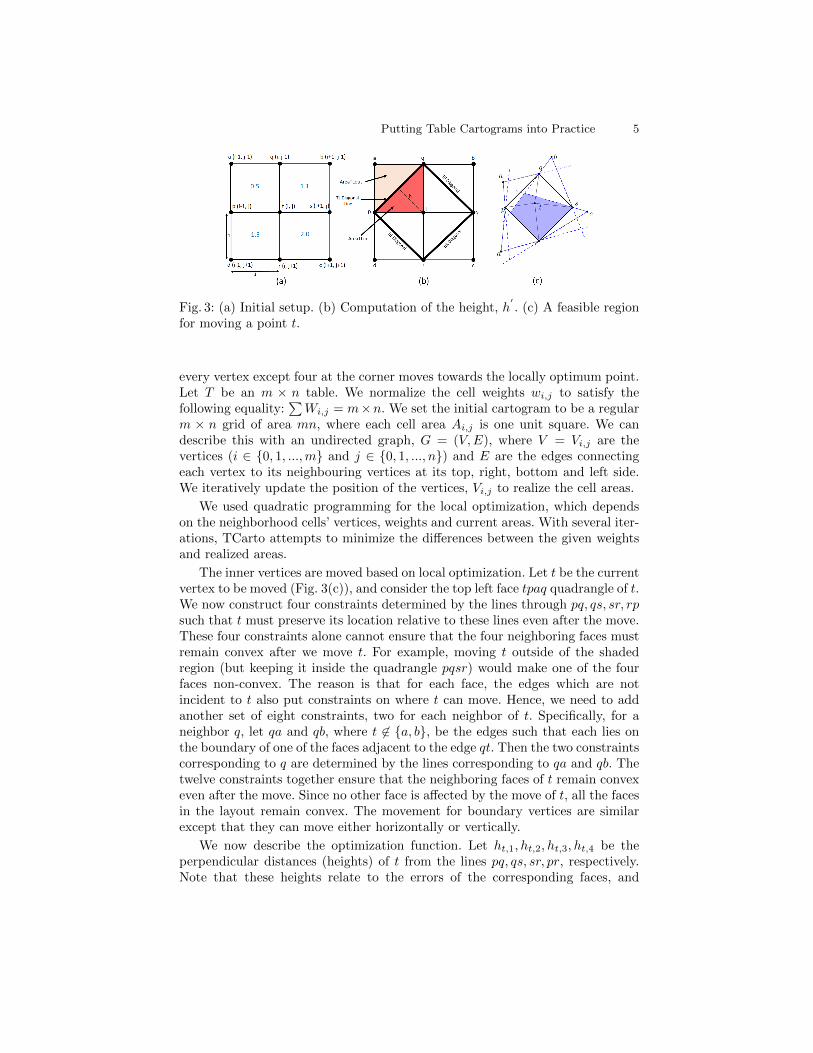
Fig. 3: (a) Initial setup. (b) Computation of the height, h′. (c) A feasible region

for moving a point t.

every vertex except four at the corner moves towards the locally optimum point.Let T be an m × n table. We normalize the cell weights wi,j to satisfy thefollowing equality:

∑Wi,j = m×n. We set the initial cartogram to be a regular

m × n grid of area mn, where each cell area Ai,j is one unit square. We candescribe this with an undirected graph, G = (V,E), where V = Vi,j are thevertices (i ∈ {0, 1, ...,m} and j ∈ {0, 1, ..., n}) and E are the edges connectingeach vertex to its neighbouring vertices at its top, right, bottom and left side.We iteratively update the position of the vertices, Vi,j to realize the cell areas.

We used quadratic programming for the local optimization, which dependson the neighborhood cells’ vertices, weights and current areas. With several iter-ations, TCarto attempts to minimize the differences between the given weightsand realized areas.

The inner vertices are moved based on local optimization. Let t be the currentvertex to be moved (Fig. 3(c)), and consider the top left face tpaq quadrangle of t.We now construct four constraints determined by the lines through pq, qs, sr, rpsuch that t must preserve its location relative to these lines even after the move.These four constraints alone cannot ensure that the four neighboring faces mustremain convex after we move t. For example, moving t outside of the shadedregion (but keeping it inside the quadrangle pqsr) would make one of the fourfaces non-convex. The reason is that for each face, the edges which are notincident to t also put constraints on where t can move. Hence, we need to addanother set of eight constraints, two for each neighbor of t. Specifically, for aneighbor q, let qa and qb, where t 6∈ {a, b}, be the edges such that each lies onthe boundary of one of the faces adjacent to the edge qt. Then the two constraintscorresponding to q are determined by the lines corresponding to qa and qb. Thetwelve constraints together ensure that the neighboring faces of t remain convexeven after the move. Since no other face is affected by the move of t, all the facesin the layout remain convex. The movement for boundary vertices are similarexcept that they can move either horizontally or vertically.

We now describe the optimization function. Let ht,1, ht,2, ht,3, ht,4 be theperpendicular distances (heights) of t from the lines pq, qs, sr, pr, respectively.Note that these heights relate to the errors of the corresponding faces, and

6 Hasan et al.

moving t would change these heights (e.g., see Figure 3(b)). We then define aset of required heights h′t,i, where 1 ≤ i ≤ 4. Here we only show how to computeh′t,1. Denote by W (tpaq) the target weight of a face tpaq, and let A(tpaq) denotearea of the face. Assume that γ = W (tpaq)− A(tpaq)−∆tpq. If γ > 0, i.e., weneed to add more area by moving t, then the required height is determined bythe equation 1

2 |pq|h′t,1 = γ+ ∆tpq, where |pq| is the Euclidean distance between

p, q. Otherwise, γ ≤ 0, i.e., we already have more than the required area. In thiscase (for simplicity) we assume that h′t,1 = ht,1. We then minimize the error∑

w∈V∑

1≤i≤4(h′w,i − hw,i)2, where V is the set of grid vertices.

Let aix + biy = ci, where 1 ≤ i ≤ 4, be the equation of four diagonallines (pq, qs, sr, rp), and let h′i be the required heights. We can thus model themovement of an inner vertex using a quadratic programming with the twelveconstraints for convexity (Fig. 3(c)) and the following optimization function.

minimize4∑

i=1

((a2ix

2

ai2+bi2

)2x2+

(b2i y

2

ai2+bi2

)2y2+ aibixy√

ai2+bi2

+ai(ci−h′

i)x√ai

2+bi2+

bi(ci−h′i)y√

ai2+bi2

)

Parallel Computing. To take advantage of parallel computing, we partitionthe vertices and distribute the load to different threads. At each iteration, wepartition the columns into k regular intervals with one column gap in between.The iteration is completed in two phases. In the first phase, each thread movestheir allocated points, and in the second phase the threads move the interleavedcolumns. We will refer to this procedure as Parallel-Opt.

The limitation of the Parallel-Opt is that if the data density is very highin a particular interval, then it would take many iterations until the points movetowards a low density region. To cope with this challenge, we take a top-downapproach, as follows. Let the input be a 2j × 2j grid. For each i from 0 to j,in the ith level we group the cells into a 2i × 2i grid and run the procedureParallel-Opt for j − log(i) + 1 iterations. Thus the major weight shift occursearly in the top levels and further refinement occurs at the bottom levels.

4 Potential Applications

Here we show some potential applications of large table cartograms (i.e., positiveevidence towards RQ1) and examine whether convexity of the cells is crucial forthese applications (i.e., RQ2).

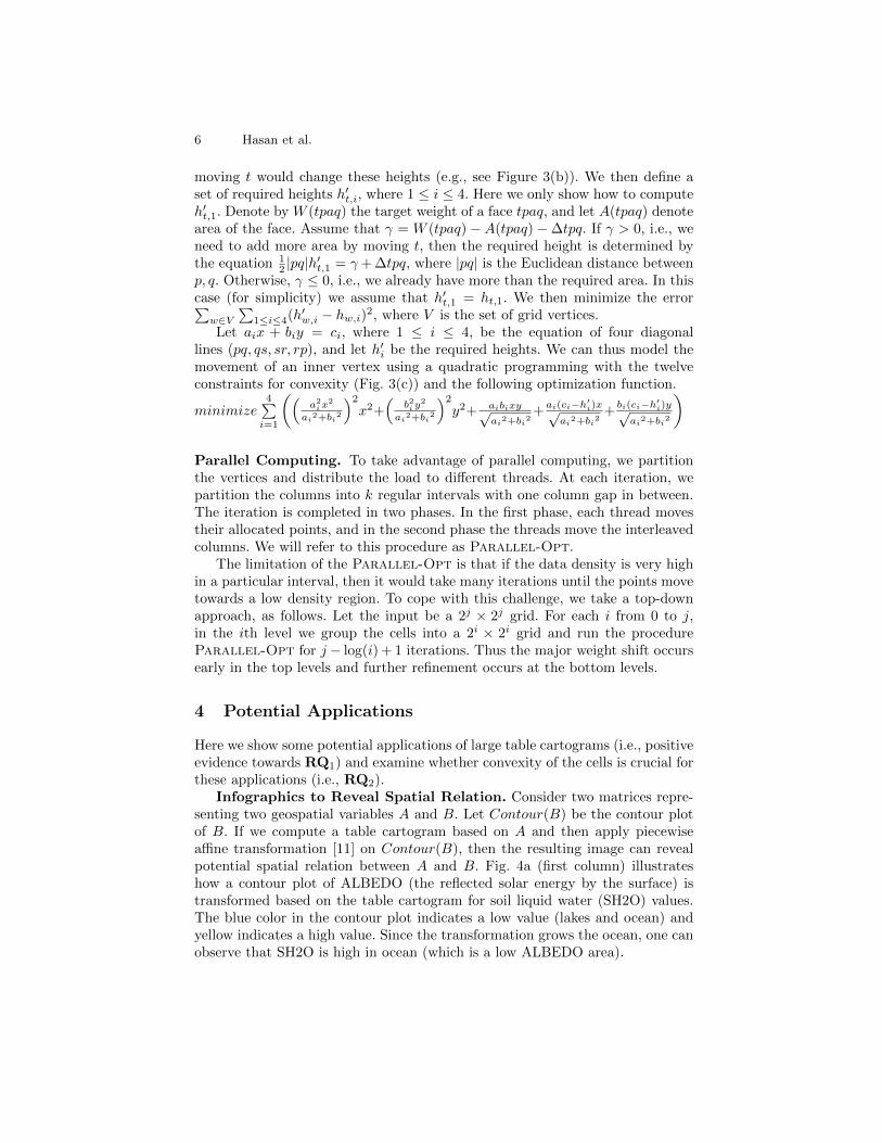
Infographics to Reveal Spatial Relation. Consider two matrices repre-senting two geospatial variables A and B. Let Contour(B) be the contour plotof B. If we compute a table cartogram based on A and then apply piecewiseaffine transformation [11] on Contour(B), then the resulting image can revealpotential spatial relation between A and B. Fig. 4a (first column) illustrateshow a contour plot of ALBEDO (the reflected solar energy by the surface) istransformed based on the table cartogram for soil liquid water (SH2O) values.The blue color in the contour plot indicates a low value (lakes and ocean) andyellow indicates a high value. Since the transformation grows the ocean, one canobserve that SH2O is high in ocean (which is a low ALBEDO area).


(a) Geospatial Correlation.

(b) Mosaic art effect.

(c) Increased illumination.

Fig. 4a shows the cartograms obtained using TCarto and FastFlow for var-ious combinations of ALBEDO (Solar Energy Reflectance), TSK (Surface SkinTemperature), PBLH (Planetary Boundary Layer Height), SH2O (Soil LiquidWater), and EMISS (Surface Emissivity). In the contour plot, blue and yellowregions are the lowest and highest values consecutively. The expansion of yellow(high value) region or shrinkage of blue (low value) region indicates potentialpositive relation. For example, see Fig. 4a (third column) for shrinkage of blue.We can infer a negative relation if the opposite happens, e.g., see Fig. 4a (first,second and fourth columns) for expansion of blue.

Discussion: Both TCarto and FastFlow shows similar transformation inregions and reveals potential relation between geospatial variables (RQ1). Thecell convexity does not appear to be a crucial phenomenon since the grid size islarge (RQ2). However, a close inspection of the grid shows that there exist majordifferences that are not readily visible in the images, but in the transformedgrid. Hence overlaying the grid on the image or placing them side-by-side mayhelp guide the interpretation when creating infographic pictures. Note that twocartograms may look very different even when their cartographic error is small(Table 1). This has also been observed by McNutt [20], but for small tables.Hence such cartogram infographics are mostly useful to spark excitement amongthe viewers, or to covey a major concept.

Different visual effects in images. Large table cartograms can potentiallybe used to create visual effects in images. Fig. 4a illustrates examples where thelightness channel of HSL (Hue, Saturation and Lightness) has been transformedusing table cartogram to expand the light illumination from the light sources.This has been achieved by overlaying a 64 × 64 grid on the image and then

8 Hasan et al.

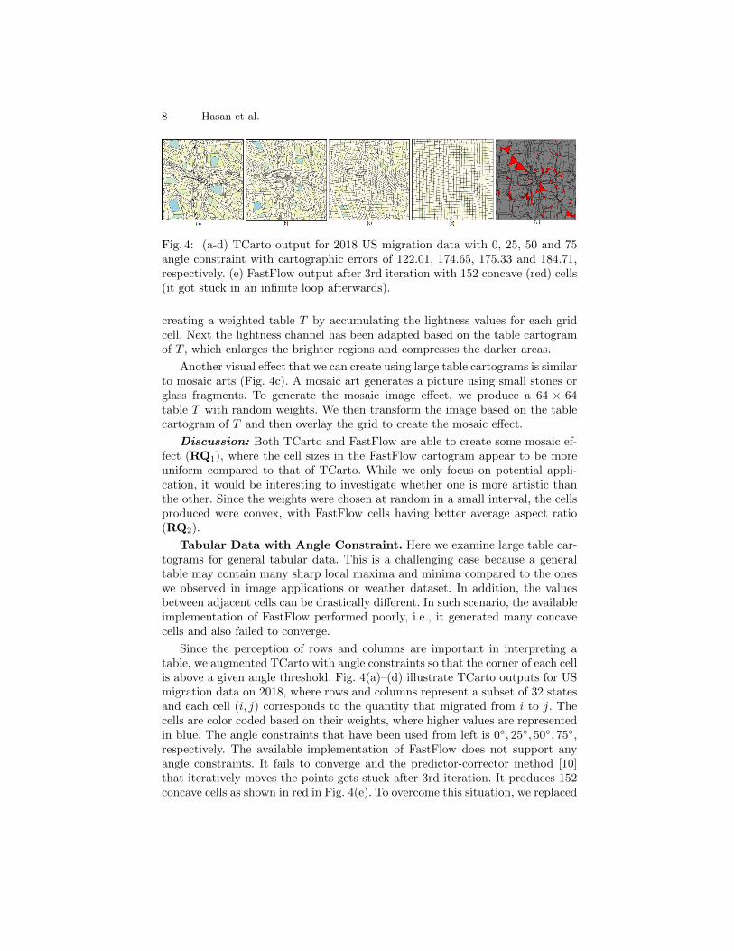
Fig. 4: (a-d) TCarto output for 2018 US migration data with 0, 25, 50 and 75angle constraint with cartographic errors of 122.01, 174.65, 175.33 and 184.71,respectively. (e) FastFlow output after 3rd iteration with 152 concave (red) cells(it got stuck in an infinite loop afterwards).

creating a weighted table T by accumulating the lightness values for each gridcell. Next the lightness channel has been adapted based on the table cartogramof T , which enlarges the brighter regions and compresses the darker areas.

Another visual effect that we can create using large table cartograms is similarto mosaic arts (Fig. 4c). A mosaic art generates a picture using small stones orglass fragments. To generate the mosaic image effect, we produce a 64 × 64table T with random weights. We then transform the image based on the tablecartogram of T and then overlay the grid to create the mosaic effect.

Discussion: Both TCarto and FastFlow are able to create some mosaic ef-fect (RQ1), where the cell sizes in the FastFlow cartogram appear to be moreuniform compared to that of TCarto. While we only focus on potential appli-cation, it would be interesting to investigate whether one is more artistic thanthe other. Since the weights were chosen at random in a small interval, the cellsproduced were convex, with FastFlow cells having better average aspect ratio(RQ2).

Tabular Data with Angle Constraint. Here we examine large table car-tograms for general tabular data. This is a challenging case because a generaltable may contain many sharp local maxima and minima compared to the oneswe observed in image applications or weather dataset. In addition, the valuesbetween adjacent cells can be drastically different. In such scenario, the availableimplementation of FastFlow performed poorly, i.e., it generated many concavecells and also failed to converge.

Since the perception of rows and columns are important in interpreting atable, we augmented TCarto with angle constraints so that the corner of each cellis above a given angle threshold. Fig. 4(a)–(d) illustrate TCarto outputs for USmigration data on 2018, where rows and columns represent a subset of 32 statesand each cell (i, j) corresponds to the quantity that migrated from i to j. Thecells are color coded based on their weights, where higher values are representedin blue. The angle constraints that have been used from left is 0◦, 25◦, 50◦, 75◦,respectively. The available implementation of FastFlow does not support anyangle constraints. It fails to converge and the predictor-corrector method [10]that iteratively moves the points gets stuck after 3rd iteration. It produces 152concave cells as shown in red in Fig. 4(e). To overcome this situation, we replaced


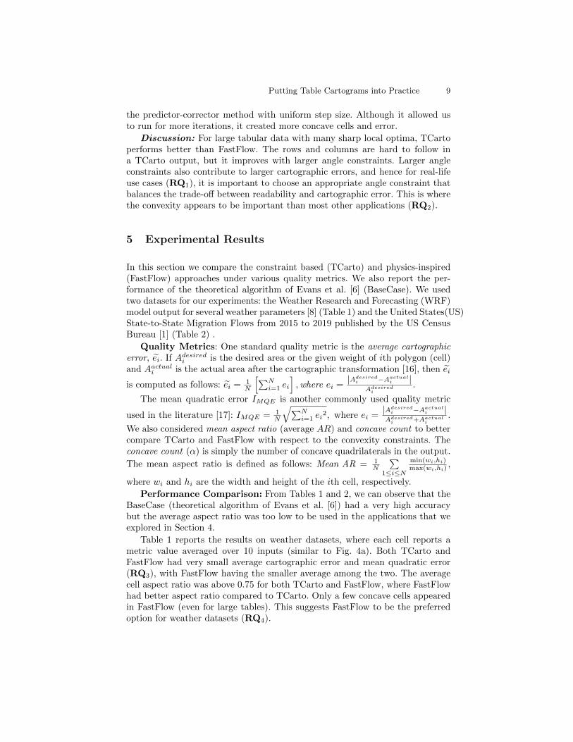
the predictor-corrector method with uniform step size. Although it allowed usto run for more iterations, it created more concave cells and error.

Discussion: For large tabular data with many sharp local optima, TCartoperforms better than FastFlow. The rows and columns are hard to follow ina TCarto output, but it improves with larger angle constraints. Larger angleconstraints also contribute to larger cartographic errors, and hence for real-lifeuse cases (RQ1), it is important to choose an appropriate angle constraint thatbalances the trade-off between readability and cartographic error. This is wherethe convexity appears to be important than most other applications (RQ2).

5 Experimental Results

In this section we compare the constraint based (TCarto) and physics-inspired(FastFlow) approaches under various quality metrics. We also report the per-formance of the theoretical algorithm of Evans et al. [6] (BaseCase). We usedtwo datasets for our experiments: the Weather Research and Forecasting (WRF)model output for several weather parameters [8] (Table 1) and the United States(US)State-to-State Migration Flows from 2015 to 2019 published by the US CensusBureau [1] (Table 2) .

Quality Metrics: One standard quality metric is the average cartographicerror, ei. If Adesired

i is the desired area or the given weight of ith polygon (cell)and Aactual

i is the actual area after the cartographic transformation [16], then ei

is computed as follows: ei = 1N

[∑Ni=1 ei

],where ei =

|Adesiredi −Aactual

i |Adesired

i

.

The mean quadratic error IMQE is another commonly used quality metric

used in the literature [17]: IMQE = 1N

√∑Ni=1 ei

2, where ei =|Adesired

i −Aactuali |

Adesiredi +Aactual

i

.

We also considered mean aspect ratio (average AR) and concave count to bettercompare TCarto and FastFlow with respect to the convexity constraints. Theconcave count (α) is simply the number of concave quadrilaterals in the output.

The mean aspect ratio is defined as follows: Mean AR = 1N

∑1≤i≤N

min(wi,hi)max(wi,hi)

,

where wi and hi are the width and height of the ith cell, respectively.

Performance Comparison: From Tables 1 and 2, we can observe that theBaseCase (theoretical algorithm of Evans et al. [6]) had a very high accuracybut the average aspect ratio was too low to be used in the applications that weexplored in Section 4.

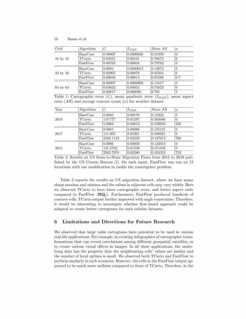
Table 1 reports the results on weather datasets, where each cell reports ametric value averaged over 10 inputs (similar to Fig. 4a). Both TCarto andFastFlow had very small average cartographic error and mean quadratic error(RQ3), with FastFlow having the smaller average among the two. The averagecell aspect ratio was above 0.75 for both TCarto and FastFlow, where FastFlowhad better aspect ratio compared to TCarto. Only a few concave cells appearedin FastFlow (even for large tables). This suggests FastFlow to be the preferredoption for weather datasets (RQ4).

10 Hasan et al.

Grid Algorithm ei IMQE Mean AR α

16 by 16BaseCase 0.00007 0.0000026 0.21039 0TCarto 0.03421 0.00161 0.76672 0FastFlow 0.00763 0.00034 0.79762 0

32 by 32BaseCase 0.0004 0.0000012 0.12073 0TCarto 0.02905 0.00076 0.82364 0FastFlow 0.00648 0.00014 0.85596 0.7

64 by 64BaseCase 0.00007 0.0000009 0.11617 0TCarto 0.03632 0.00052 0.75623 0FastFlow 0.00817 0.000095 0.791 5

Table 1: Cartographic error (ei), mean quadratic error (IMQE), mean aspectratio (AR) and average concave count (α) for weather dataset.

Year Algorithm ei IMQE Mean AR α

2019BaseCase 0.0083 0.00170 0.12322 0TCarto 119.777 0.01297 0.563086 0FastFlow 5.9962 0.00813 0.539933 346



Table 2: Results on US State-to-State Migration Flows from 2015 to 2019 pub-lished by the US Census Bureau [1]. On each input, FastFlow was run on 15iterations with our modification to tackle the convergence problem.

Table 2 reports the results on US migration dataset, where we have manysharp maxima and minima and the values in adjacent cells may vary widely. Herewe observed TCarto to have lower cartographic error, and better aspect ratiocompared to FastFlow (RQ4). Furthermore, FastFlow produced hundreds ofconcave cells. TCarto output further improved with angle constraints. Therefore,it would be interesting to investigate whether flow-based approach could beadapted to create better cartograms for such tabular datasets.

6 Limitations and Directions for Future Research

We observed that large table cartograms have potential to be used in variousreal-life applications. For example, in creating infographics of cartographic trans-formations that can reveal correlations among different geospatial variables, orto create various visual effects in images. In all these applications, the under-lying data has the property that the neighbouring cells’ values are similar andthe number of local optima is small. We observed both TCarto and FastFlow toperform similarly in such scenarios. However, the cells in the FastFlow output ap-peared to be much more uniform compared to those of TCarto. Therefore, in the


image-based applications, the images were less distorted in the FastFlow output.Since such visual observation is subject to human interpretation, it would thusbe interesting to devise performance metrics that takes also the image distortioninto account.

In general, for large tabular dataset with many local optima with large spikesand large value differences between adjacent cells, neither the TCarto nor Fast-Flow produced appealing output. However, TCarto with angle constraints im-proved the readability of the table with the expense of introducing cartographicerror. This suggests the importance of choosing an appropriate angle constraintthat allows users to follow the rows and columns, as well as to understand therelative cell areas, peaks and valley regions.

Since we invested our effort largely on exploring the scope of table car-tograms, we did not focus on conducting controlled user studies or interviewswith the domain experts (artists or photographers) to evaluate the artistic qual-ity of the outputs generated by TCarto and FastFlow. For weather dataset, suchinterviews with meteorologists may potentially help understand which techniquereveals the relation among various weather parameters better than the other. Itwould also be interesting to examine how cartogram based approach compareswith today’s artificial intelligence based approaches for creating digital arts. BothTCarto and FastFlow could handle large tables (128× 128, Fig. 4c), but none ofthe current implementations leverages GPU computation. Thus it would be aninteresting avenue to explore whether GPUs can be leveraged to compute tablecartograms in interaction time.

Both the constraint-based approach and physics-inspired cartographic maptransformation are effective in generating large scale cartograms (with low carto-graphic error, good cell aspect ratio and few concave cells) for image and weatherdatasets. However, for data tables with large number of local optima and highspikes, we observed constraint based optimization to work better than flow-basedapproach. We believe our investigation on the scope and opportunities relatinglarge table cartograms would inspire future research on cartogram based imagetransformation.

References

1. Bureau, U.C.: State-to-state migration flows. https://www.census.gov/data/tables/time-series/demo/geographic-mobility/state-to-state-migration.html, last Revised Nov2020

2. Cano, R.G., Buchin, K., Castermans, T., Pieterse, A., Sonke, W., Speckmann,B.: Mosaic drawings and cartograms. In: Computer Graphics Forum. vol. 34, pp.361–370. Wiley Online Library (2015)

3. Cauvin, C., Schneider, C.: Cartographic transformations and the piezopleth mapsmethod. The Cartographic Journal 26(2), 96–104 (1989)

4. Dougenik, J.A., Chrisman, N.R., Niemeyer, D.R.: An algorithm to construct con-tinuous area cartograms. The Professional Geographer 37(1), 75–81 (1985)

5. Espenant, J., Mondal, D.: Streamtable: An area proportional visualization for ta-bles with flowing streams. In: European Workshop on Computational Geometry.pp. 28:1–28:7 (2021), arXiv:https://arxiv.org/abs/2103.15037

12 Hasan et al.

6. Evans, W., Felsner, S., Kaufmann, M., Kobourov, S.G., Mondal, D., Nishat, R.I.,Verbeek, K.: Table cartogram. Computational Geometry 68, 174–185 (2018)

7. Fletcher, R.: A general quadratic programming algorithm. IMA Journal of AppliedMathematics 7(1), 76–91 (1971)

8. Foundation, N.S.: Weather research and forecasting model.https://www.mmm.ucar.edu/weather-research-and-forecasting-model, last Ac-cessed Jun 2019

9. Gastner, M.T., Newman, M.E.: Diffusion-based method for producing density-equalizing maps. Proceedings of the National Academy of Sciences 101(20), 7499–7504 (2004)

10. Gastner, M.T., Seguy, V., More, P.: Fast flow-based algorithm for creating density-equalizing map projections. Proceedings of the National Academy of Sciences115(10), E2156–E2164 (2018)

11. Hartley, R., Zisserman, A.: Multiple View Geometry in Computer Vision. Cam-bridge University Press (2003)

12. Henriques, R., Bacao, F., Lobo, V.: Carto-SOM: cartogram creation using self-organizing maps. International Journal of Geographical Information Science 23(4),483–511 (2009)

13. Hildreth, C., et al.: A quadratic programming procedure. Naval research logisticsquarterly 4(1), 79–85 (1957)

14. House, D.H., Kocmoud, C.J.: Continuous cartogram construction. In: ProceedingsVisualization’98. pp. 197–204. IEEE (1998)

15. Inoue, R., Li, M.: Optimization-based construction of quadrilateral table car-tograms. ISPRS International Journal of Geo-Information 9(1), 43 (2020)

16. Inoue, R., Shimizu, E.: A new algorithm for continuous area cartogram construc-tion with triangulation of regions and restriction on bearing changes of edges.Cartography and Geographic Information Science 33(2), 115–125 (2006)

17. Keim, D.A., North, S.C., Panse, C.: Cartodraw: A fast algorithm for generatingcontiguous cartograms. IEEE transactions on visualization and computer graphics10(1), 95–110 (2004)

18. Keim, D.A., Panse, C., North, S.C.: Medial-axis-based cartograms. IEEE computergraphics and applications 25(3), 60–68 (2005)

19. McNutt, A., Kindlmann, G.: A minimally constrained optimization algo-rithm for table cartograms. IEEEVIS InfoVis Posters (2020), OSF Preprints,https://doi.org/10.31219/osf.io/kem6j

20. McNutt, A.: What are table cartograms good for anyway? an algebraic analysis.Eurographics Conference on Visualization (EuroVis) 40 (2021), to appear.

21. Nusrat, S., Kobourov, S.: The state of the art in cartograms. In: Computer Graph-ics Forum. vol. 35, pp. 619–642. Wiley Online Library (2016)

22. Sun, S.: A fast, free-form rubber-sheet algorithm for contiguous area cartograms.International Journal of Geographical Information Science 27(3), 567–593 (2013)

23. Tobler, W.: Thirty five years of computer cartograms. ANNALS of the Associationof American Geographers 94(1), 58–73 (2004)

24. Tutte, W.T.: How to draw a graph. vol. 3, pp. 743–767. Wiley Online Library(1963)

25. Winter, M.J.: Diffusion cartograms for the display of periodic table data. Journalof Chemical Education 88(11), 1507–1510 (2011)

putting table cartograms into practice

Documents