p(y g y p(g y - calvin collegerpruim/courses/s241/s17/test-info/test02... ·...

10. INDEX 241

• G4 = green from 1994 bag

• G6 = green from 1996 bag

• Y4 = yellow from 1994 bag

• Y6 = yellow from 1996 bag

Then our question becomes

P(Y4 and G6 | (Y4 and G6) or (Y6 and G4)) =P(Y4 and G6)

P((Y4 and G6) or (Y6 and G4))

=P(Y4 and G6)

P(Y4 and G6) + P(Y6 and G4)

The individual probabilities can be worked out as

P(Y4 and G6) = P(Y4) · P(G6 | Y4) = .20 · .20 = 0.04

P(Y6 and G4) = P(Y6) · P(G4 | Y6) = .14 · .10 = 0.014

Putting this all together we get

0.2 * 0.2/(0.2 * 0.2 + 0.14 * 0.1)

## [1] 0.7407

A tree diagram could be used to depict these probabilities as well.

4.1

f <- makeFun((5/4 - x^3) * (abs(x - 0.5) <= 0.5) ~ x)

plotFun(f(x) ~ x, x.lim = c(-1, 2)) # quick plot to make sure things look correct.

F <- antiD(f(x) ~ x)

# part a: f(x) >=0, so we just need to check that the total area is 1

F(1) - F(0) == 1

## [1] TRUE

F(1/2) - F(0) # part b

## [1] 0.6094

F(1) - F(1/2) # part c

## [1] 0.3906

F(1/2) - F(1/2) # part d

## [1] 0

Math 241 : Spring 2017 : Pruim Last Modified: March 9, 2017

242 10. INDEX

xf(

x)

0.0

0.5

1.0

−0.5 0.0 0.5 1.0 1.5

4.2

• P(X ≤ 1) = 12 · 1 ·

12 = 1

4

• P(X ≤ 2) = 1− P(X ≥ 2) = 1− 12 · 2 ·

13 = 1− 1

3 = 23 .

• The median m is a number between 1 and 2 and satisfies 12 = P(X ≥ m) = 1

2 (4−m) 4−m6 . Solving for m

we get m = 4−√

6 = 1.551.

4.3 The integrals are easy enough to do by hand, but here is the R code to compute them.

k <- makeFun( 1 - x^2 ~ x )

K <- antiD( k(x) ~ x )

area <- K(1) - K(-1); area

## [1] 1.333

f <- makeFun( (1 - x^2)/A ~ x, A=area )


F(1) - F(-1) # this should be 1 if we have done things right

## [1] 1

G <- antiD( x * f(x) ~ x )

H <- antiD( x^2 * f(x) ~ x )

m <- G(1) - G(-1); m # E(X)

## [1] 0

H(1) - H(-1) # E(X^2)

## [1] 0.2

H(1) - H(-1) - m^2 # Var(X)

## [1] 0.2

Last Modified: March 9, 2017 Stat 241 : Spring 2017 : Pruim

10. INDEX 243

4.4

# mean:

m <- antiD(x * dtriangle(x, 0, 10, 4) ~ x, lower.bound = 0)(10)

m

## [1] 4.667

# variance:

antiD(x^2 * dtriangle(x, 0, 10, 4) ~ x, lower.bound = 0)(10) - m^2

## [1] 4.222

# median

qtriangle(0.5, 0, 10, 4)

## [1] 4.523

4.5

# mean:

m <- antiD(x * dunif(x, 0, 10) ~ x, lower.bound = 0)(10)

m

## [1] 5

# variance:

antiD(x^2 * dunif(x, 0, 10) ~ x, lower.bound = 0)(10) - m^2

## [1] 8.333

4.6

antiD(x * dexp(x, 4) ~ x, lower.bound = 0)(Inf)

## [1] 0.25

antiD(x * dexp(x, 10) ~ x, lower.bound = 0)(Inf)

## [1] 0.1

antiD(x * dexp(x, 1/5) ~ x, lower.bound = 0)(Inf)

## [1] 5


244 10. INDEX

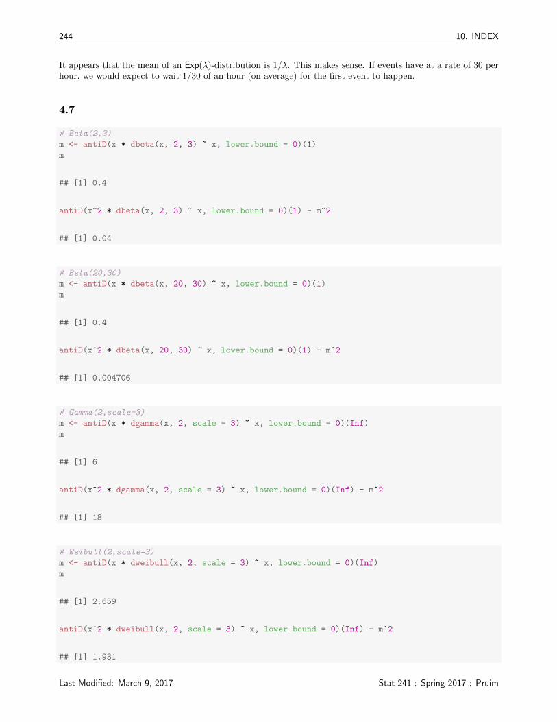
It appears that the mean of an Exp(λ)-distribution is 1/λ. This makes sense. If events have at a rate of 30 perhour, we would expect to wait 1/30 of an hour (on average) for the first event to happen.

4.7

# Beta(2,3)

m <- antiD(x * dbeta(x, 2, 3) ~ x, lower.bound = 0)(1)

m

## [1] 0.4

antiD(x^2 * dbeta(x, 2, 3) ~ x, lower.bound = 0)(1) - m^2

## [1] 0.04

# Beta(20,30)

m <- antiD(x * dbeta(x, 20, 30) ~ x, lower.bound = 0)(1)

m

## [1] 0.4

antiD(x^2 * dbeta(x, 20, 30) ~ x, lower.bound = 0)(1) - m^2

## [1] 0.004706

# Gamma(2,scale=3)

m <- antiD(x * dgamma(x, 2, scale = 3) ~ x, lower.bound = 0)(Inf)

m

## [1] 6

antiD(x^2 * dgamma(x, 2, scale = 3) ~ x, lower.bound = 0)(Inf) - m^2

## [1] 18

# Weibull(2,scale=3)

m <- antiD(x * dweibull(x, 2, scale = 3) ~ x, lower.bound = 0)(Inf)

m

## [1] 2.659

antiD(x^2 * dweibull(x, 2, scale = 3) ~ x, lower.bound = 0)(Inf) - m^2

## [1] 1.931


10. INDEX 245

4.8

pexp(1, 2) - pexp(0.5, 2)

## [1] 0.2325

pbeta(1, 3, 2) - pbeta(0.5, 3, 2)

## [1] 0.6875

pnorm(1, 1, 2) - pnorm(0.5, 1, 2)

## [1] 0.09871

pweibull(1, 2, scale = 1/2) - pweibull(0.5, 2, scale = 1/2)

## [1] 0.3496

pgamma(1, 2, scale = 1/2) - pgamma(0.5, 2, scale = 1/2)

## [1] 0.3298

4.9

a) The method of moments fit for λ comes from solving 1λ = x for λ, so λ̂ = 1

x

lambda.hat <- 1/mean(~speed, data = Wind)

lambda.hat

## [1] 0.1688

b) fitdistr(Wind$speed, "exponential")

## rate

## 0.168770

## (0.001041)

c) They are the same in this case.

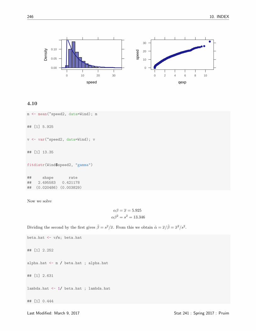
d) This fit is not that great.

histogram(~speed, data = Wind, fit = "exponential")

qqmath(~speed, data = Wind, distribution = qexp)


246 10. INDEX

speed

Den

sity

0.00

0.05

0.10

0 10 20 30

qexp

spee

d

0

10

20

30

0 2 4 6 8 10

4.10

m <- mean(~speed2, data=Wind); m

## [1] 5.925

v <- var(~speed2, data=Wind); v

## [1] 13.35

fitdistr(Wind$speed2, "gamma")

## shape rate

## 2.495583 0.421178

## (0.020486) (0.003829)

Now we solve

αβ = x = 5.925

αβ2 = s2 = 13.346

Dividing the second by the first gives β̂ = s2/x. From this we obtain α̂ = x/β̂ = x2/s2.

beta.hat <- v/m; beta.hat

## [1] 2.252

alpha.hat <- m / beta.hat ; alpha.hat

## [1] 2.631

lambda.hat <- 1/ beta.hat ; lambda.hat

## [1] 0.444


10. INDEX 247

The fitted values are similar to but not identical to the maximum likelihood estimates.

4.11 We can recycle some work from the previous problem to quickly obtain the method of moments fit forthe Gamma distribution:

m <- 10.2

v <- 5.1^2

beta.hat <- v/m; beta.hat

## [1] 2.55

alpha.hat <- m / beta.hat ; alpha.hat

## [1] 4

lambda.hat <- 1/ beta.hat ; lambda.hat

## [1] 0.3922

For the Rayliegh distribution we solve β̂√π

2 = x for β̂ and get

β̂ =2x√π

=2 · 10.2√

π= 11.509

4.12 The distribution is skewed and non-negative, so a gamma or Weibull seems like a good thing to try.

fitdistr(Baby$cry.count, "gamma")

## shape rate

## 12.6338 0.7330

## ( 2.8609) ( 0.1693)

fitdistr(Baby$cry.count, "Weibull")

## shape scale

## 3.5842 19.1020

## ( 0.4245) ( 0.9178)

histogram(~cry.count, data = Baby, fit = "gamma", main = "Gamma")

histogram(~cry.count, data = Baby, fit = "Weibull", main = "Weibull")


248 10. INDEX

Gamma

cry.count

Den

sity

0.00

0.02

0.04

0.06

0.08

10 15 20 25 30

Weibull

cry.count

Den

sity

0.00

0.02

0.04

0.06

0.08

10 15 20 25 30

4.13

qqmath(~age | substance, data = HELPrct)

qnorm

age

20

30

40

50

60

−3 −1 0 1 2 3

alcohol

−3 −1 0 1 2 3

cocaine

−3 −1 0 1 2 3

heroin

The qq-plot for the alchol group looks good. The other two (especially cocaine) show signs of skew – indicatedby the curve to the qq plot.

densityplot(~age | substance, data = HELPrct)

age

Den

sity

0.00

0.02

0.04

0.06

10 30 50

alcohol

10 30 50

cocaine

10 30 50

heroin

4.14 a) Y b) V c) Z d) W e) X f) U


10. INDEX 249

4.15 ∫ ∞−∞

(x− µX)2f(x) dx =

∫ ∞−∞

(x2 − 2µXx+ µ2X)f(x) dx

=

∫ ∞−∞

(x2f(x) dx− 2µX

∫ ∞−∞

xf(x) dx+ µ2X

∫ ∞−∞

f(x) dx

= Var(X)− 2µ2X + µ2

X

= Var(X)− E(X)2

4.16

a) (68 - 64.3)/2.6

## [1] 1.423

b) (74 - 70)/2.8

## [1] 1.429

c) It’s pretty close, but the z-score for the man is slightly larger, so it is slightly more unusual for a man tobe that tall.

d) 64.3 + 2 * 2.6

## [1] 69.5

e) 70 + 2 * 2.8

## [1] 75.6

4.17

a) 1 - pnorm(70, mean = 64.3, sd = 2.6)

## [1] 0.01418

b) 1 - pnorm(76, mean = 70, sd = 2.8)

## [1] 0.01606

c) qnorm(0.75, mean = 70, sd = 2.8)

## [1] 71.89


250 10. INDEX

d) qnorm(0.3, mean = 64.3, sd = 2.6)

## [1] 62.94

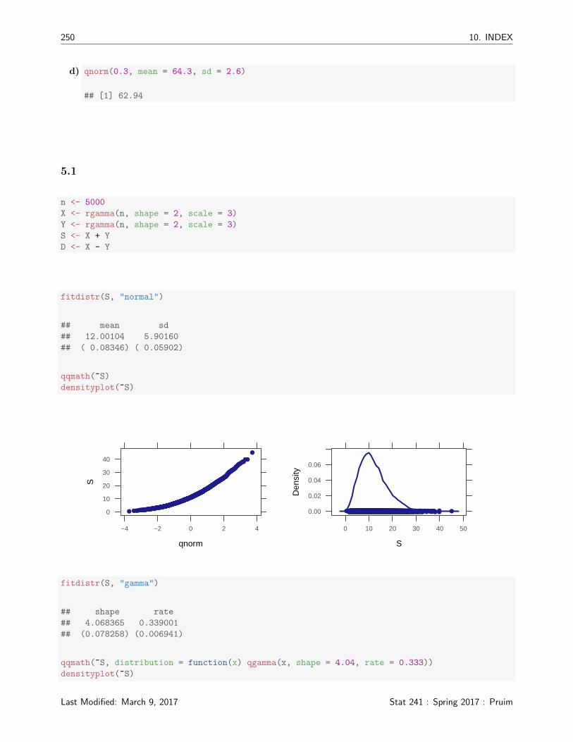
5.1

n <- 5000

X <- rgamma(n, shape = 2, scale = 3)

Y <- rgamma(n, shape = 2, scale = 3)

S <- X + Y

D <- X - Y

fitdistr(S, "normal")

## mean sd

## 12.00104 5.90160

## ( 0.08346) ( 0.05902)

qqmath(~S)

densityplot(~S)

qnorm

S

0

10

20

30

40

−4 −2 0 2 4

S

Den

sity

0.00

0.02

0.04

0.06

0 10 20 30 40 50

fitdistr(S, "gamma")

## shape rate

## 4.068365 0.339001

## (0.078258) (0.006941)

qqmath(~S, distribution = function(x) qgamma(x, shape = 4.04, rate = 0.333))

densityplot(~S)


10. INDEX 251

function(x) qgamma(x, shape = 4.04, rate = 0.333)

S

0

10

20

30

40

0 10 20 30 40 50

S

Den

sity

0.00

0.02

0.04

0.06

0 10 20 30 40 50

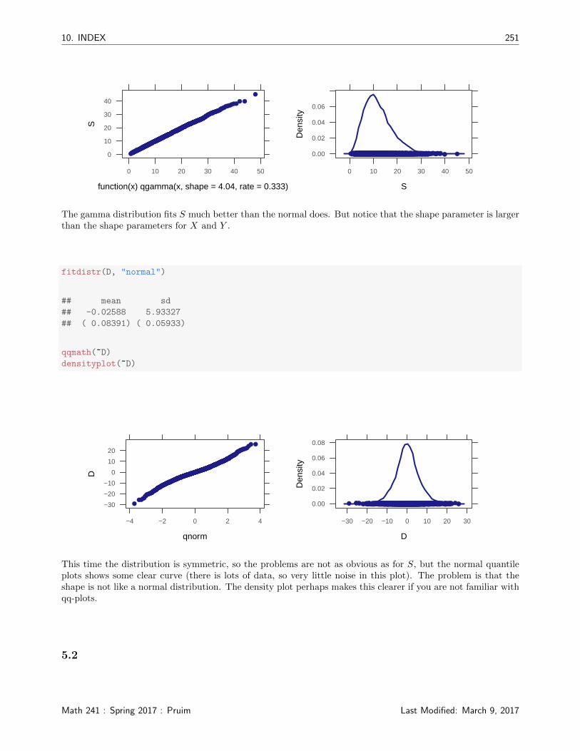
The gamma distribution fits S much better than the normal does. But notice that the shape parameter is largerthan the shape parameters for X and Y .

fitdistr(D, "normal")

## mean sd

## -0.02588 5.93327

## ( 0.08391) ( 0.05933)

qqmath(~D)

densityplot(~D)

qnorm

D

−30

−20

−10

0

10

20

−4 −2 0 2 4

D

Den

sity

0.00

0.02

0.04

0.06

0.08

−30 −20 −10 0 10 20 30

This time the distribution is symmetric, so the problems are not as obvious as for S, but the normal quantileplots shows some clear curve (there is lots of data, so very little noise in this plot). The problem is that theshape is not like a normal distribution. The density plot perhaps makes this clearer if you are not familiar withqq-plots.

5.2


252 10. INDEX

1 - pnorm(140, mean = 110, sd = 15) # P(X > 140)

## [1] 0.02275

1 - pnorm(140, mean = 100, sd = 20) # P(Y > 140)

## [1] 0.02275

1 - pnorm(150, mean = 110, sd = 15) # P(X > 150)

## [1] 0.00383

1 - pnorm(150, mean = 100, sd = 20) # P(Y > 150)

## [1] 0.00621

X + Y ∼ Norm(210, 25) because 110 + 100 = 210 and 152 + 202 = 252. So P(X + Y ≥ 250) is

1 - pnorm(250, 210, 25)

## [1] 0.0548

X − Y ∼ Norm(10, 25) because 110− 100 = 210 and 152 + 202 = 252. So P(X − Y ≥ 0) is

1 - pnorm(0, 10, 25)

## [1] 0.6554

5.3


10. INDEX 253

# part a

c(mean = 54 + 48, sd = sqrt(12^2 + 9^2))

## mean sd

## 102 15

# part b

c(mean = 2 * 54, sd = 2 * 12)

## mean sd

## 108 24

# part c

c(mean = 2 * 54 + 3 * 48, sd = sqrt(2^2 * 12^2 + 3^2 * 9^2))

## mean sd

## 252.00 36.12

# part d

c(mean = 2 * 54 - 3 * 48, sd = sqrt(2^2 * 12^2 + (-3)^2 * 9^2))

## mean sd

## -36.00 36.12

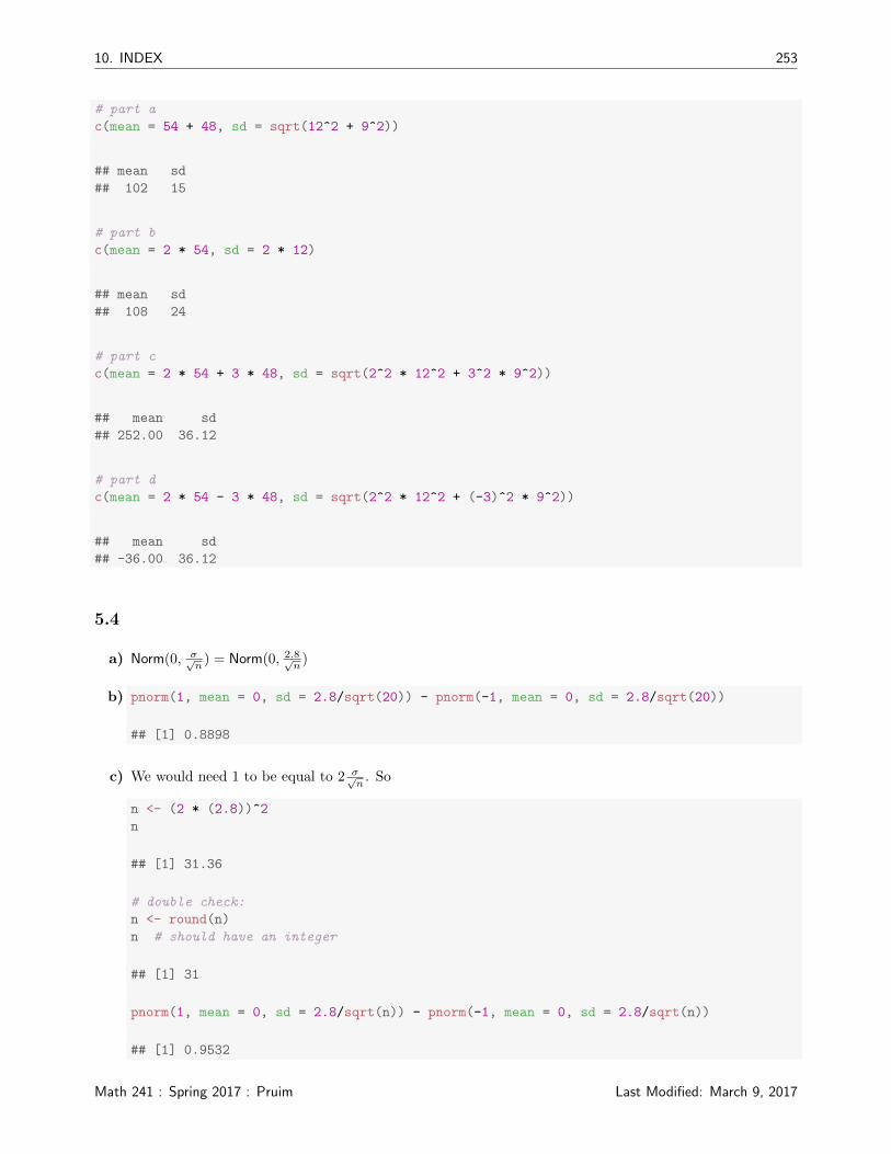
5.4

a) Norm(0, σ√n

) = Norm(0, 2.8√n

)

b) pnorm(1, mean = 0, sd = 2.8/sqrt(20)) - pnorm(-1, mean = 0, sd = 2.8/sqrt(20))

## [1] 0.8898

c) We would need 1 to be equal to 2 σ√n

. So

n <- (2 * (2.8))^2

n

## [1] 31.36

# double check:

n <- round(n)

n # should have an integer

## [1] 31

pnorm(1, mean = 0, sd = 2.8/sqrt(n)) - pnorm(-1, mean = 0, sd = 2.8/sqrt(n))

## [1] 0.9532


254 10. INDEX

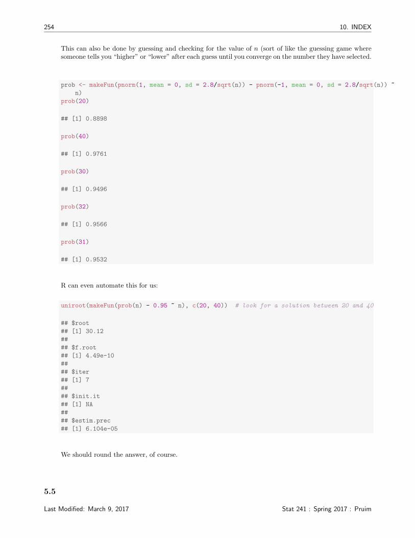
This can also be done by guessing and checking for the value of n (sort of like the guessing game wheresomeone tells you “higher” or “lower” after each guess until you converge on the number they have selected.

prob <- makeFun(pnorm(1, mean = 0, sd = 2.8/sqrt(n)) - pnorm(-1, mean = 0, sd = 2.8/sqrt(n)) ~

n)

prob(20)

## [1] 0.8898

prob(40)

## [1] 0.9761

prob(30)

## [1] 0.9496

prob(32)

## [1] 0.9566

prob(31)

## [1] 0.9532

R can even automate this for us:

uniroot(makeFun(prob(n) - 0.95 ~ n), c(20, 40)) # look for a solution between 20 and 40

## $root

## [1] 30.12

##

## $f.root

## [1] 4.49e-10

##

## $iter

## [1] 7

##

## $init.it

## [1] NA

##

## $estim.prec

## [1] 6.104e-05

We should round the answer, of course.

5.5


10. INDEX 255

SE <- 1.7 / sqrt(25) ; SE # standard error

## [1] 0.34

ME <- 2 * SE; ME # margin of error

## [1] 0.68

8.5 + c(-1,1) * ME # approx 95% CI

## [1] 7.82 9.18

5.6 Here’s a fancy version that gets all the answers at once. (You didn’t need to know you could do it this way,but R is pretty handy this way.)

answers <- qt(c(0.975, 0.975, 0.99, 0.95, 0.995, 0.975), df = c(3, 23, 14, 19, 11, 122))

names(answers) <- letters[1:length(answers)]

answers

## a b c d e f

## 3.182 2.069 2.624 1.729 3.106 1.980

5.7

t.test(~strideRate, data = ex07.37, conf.level = 0.98)

##

## One Sample t-test

##

## data: ex07.37$strideRate

## t = 51, df = 19, p-value <2e-16

## alternative hypothesis: true mean is not equal to 0

## 98 percent confidence interval:

## 0.8795 0.9715

## sample estimates:

## mean of x

## 0.9255

The normal quantile plot is OK but not great. There are some flat spots in the plot indicating ties. Thisis probably because the number of steps was counted over a short length of time, so the underlying data isprobably discrete – leading to the ties. But the distribution is unimodal and not heavily skewed. With a samplesize of 20 we can probably proceed cautiously. (In practice, we might want to confirm the results with a methodtaht doesn’t require such a strong normality assumption, but we don’t know any of those methods yet.)

5.8

a) 4-year-old fish Here’s the 95% confidence interval.


256 10. INDEX

confint(t.test(~Length, data = fish4))

## mean of x lower upper level

## 1 153.8 150.7 157 0.95

We must be willing to assume that the sampling process produces a reasonable approximation to a random(iid) sample. (We might need to know something about how the fish were captured to decide if this isreasonable. A method of catching fish that works better for larger fish than for smaller fish, or vice versa,would be problematic.) A normal-quantile plot doesn’t suggest any reason to be overly worried about thenormality assumption.

qqmath(~Length, data = fish4)

qnorm

Leng

th

140

150

160

170

−2 −1 0 1 2

int <- confint(t.test( ~Length, data=fish4))

int


## 1 153.8 150.7 157 0.95

lo <- int[2]

hi <- int[3]

tally ( ~ ( lo < Length & Length < hi ), data=fish4 )

## (lo < Length & Length < hi)

## TRUE FALSE

## 0 1

None of the fish have a length inside the confidence interval – this is far below 95%. This is NOT aproblem. The confidence interval is not about the lengths of individual fish, it is about the mean for thepopulation of fish. (Side note: It looks like many of the measurements were rounded to the nearest 10 cm,and since our confidence interval fit between 150 and 160, there were no fish of those lengths.)

b) 3-year-old fish


10. INDEX 257

fish3 <- subset(lakemary, Age==3) # note the double == here

qqmath(~Length, data=fish3)

int <- confint(t.test(~Length, data=fish3))

int


## 1 134.9 129.4 140.4 0.95

lo <- int[2]; hi <- int[3]

lo

## lower

## 1 129.4

hi

## upper

## 1 140.4

tally ( ~ ( lo < Length & Length < hi ), data=fish3 )

## (lo < Length & Length < hi)

## TRUE FALSE

## 1 0

qnorm

Leng

th

120

130

140

150

−2 −1 0 1 2

c) Since the two confidence intervals do not overlap, we have a pretty strong indication that the 4-year-oldsare (on average) longer. This isn’t really the right way to test for this – we’ll learn better ways soon.

Here is a plot that shows how length varies by age.

bwplot(Length ~ factor(Age), data = lakemary)

xyplot(Length ~ factor(Age), data = lakemary, cex = 2, alpha = 0.3)


258 10. INDEX

Leng

th

100

150

1 2 3 4 5 6

factor(Age)

Leng

th

100

150

1 2 3 4 5 6

5.9

SE <- 3.1 / sqrt(8); SE # standard error

## [1] 1.096

t_star <- qt( .975, df=7 ); t_star # critical value

## [1] 2.365

me <- t_star * SE; me # margin of error

## [1] 2.592

30.2 + c(-1,1) * me # the 95% confidence interval

## [1] 27.61 32.79

5.10

qqmath(~polymer, data = Paper)

densityplot(~polymer, data = Paper)

t.test(~polymer, data = Paper)

##

## One Sample t-test

##

## data: Paper$polymer

## t = 120, df = 16, p-value <2e-16

## alternative hypothesis: true mean is not equal to 0

## 95 percent confidence interval:

## 430.5 446.1

## sample estimates:

## mean of x

## 438.3


10. INDEX 259

qnorm

poly

mer

420

430

440

450

460

−2 −1 0 1 2

polymer

Den

sity

0.000

0.005

0.010

0.015

0.020

400 420 440 460 480

The tails of the sample distribution do not stretch quite as far as we would expect for a normal distribution,but the distribution is unimodal and not heavily skewed, so we are probably still OK.

5.11 Bob’s interval will be wider because he used a higher level of confidence. (This will cause t∗ to be larger.They will both have the same standard error.)

5.12 We would expect the two standard deviations to be fairly close, but since Denise has quite a bit moredata, her standard error will be smaller. This will make her interval narrower. So Charlie’s interval will bewider, unless Charlie gets an unusually small standard deviation and Denise gets an unusually large standarddeviation.

5.13 Answers will vary.

5.14

a) P(none defective) = P(all are good) = 0.9510 = 0.599 = 59.9%

b) Even though only 5% are defective, nearly 14% fail the quality control:

P(fail test) = P(good and fail) + P(bad and fail)

= P(good) P(fail | good) + P(bad) P(fail | bad)

= 0.95(0.10) + 0.05(.80) = 0.095 + 0.04 = 0.135 = 13.5%

c) If a part passes QC, the probability that it is defective drops from 5% to just over 1%:

P(bad | pass) =P(bad and pass)

P(pass)

=0.05(0.20)

0.865= 0.01156

The cost to get this improvement in quality is the cost of the QC test plus the cost of discarding 9.5% ofgood parts in the QC process.

d)P(bad | fail) = P(bad and fail) = P(fail) = 0.04/(0.04 + 0.095) = 0.296

0.04/(0.04 + 0.095)

## [1] 0.2963


260 10. INDEX

5.15

xD

ensi

ty

0.00

0.05

0.10

0.15

0.20

0.25

0.30

0 2 4 6 8

The important feature to get right is the direction of the skew.

5.16


10. INDEX 261

favstats( ~ length, data=KidsFeet )

## min Q1 median Q3 max mean sd n missing

## 21.6 24 24.5 25.6 27.5 24.72 1.318 39 0

x_bar <- 24.72

n <- 39; n

## [1] 39

s <- 1.32; s

## [1] 1.32

SE <- s / sqrt(n) ; SE

## [1] 0.2114

t_star <- qt( .95, df=38 ) ; t_star

## [1] 1.686

me <- t_star * SE; me

## [1] 0.3564

interval( t.test( ~length, data=KidsFeet) )

## Error in eval(expr, envir, enclos): could not find function "interval"

qqmath( ~length, data=KidsFeet )

qnorm

leng

th

22

23

24

25

26

27

−2 −1 0 1 2

The normal-quantile plot does not reveal any causes for concern, but we might be concerned that the distribu-tions for boys and girls are different. Let’s do a graphical check to see if that is a problem.


262 10. INDEX

bwplot(length ~ sex, data = KidsFeet)

densityplot(~length, groups = sex, data = KidsFeet)le

ngth

22

23

24

25

26

27

B G

length

Den

sity

0.0

0.1

0.2

0.3

20 22 24 26 28

Indeed, it appears that the girls’ feet are on average a bit shorter, so perhaps we should create a confidenceintervals separately for each group. Now you have two problems. You can get started with

favstats(length ~ sex, data = KidsFeet)

## sex min Q1 median Q3 max mean sd n missing

## 1 B 22.9 24.35 24.95 25.8 27.5 25.11 1.217 20 0

## 2 G 21.6 23.65 24.20 25.1 26.7 24.32 1.330 19 0

5.17

f <- makeFun( 4*(x-x^3) ~ x )

F <- antiD( f(x) ~ x )

xF <- antiD( x * f(x) ~ x )

xxF <- antiD( x^2 * f(x) ~ x )

F(1) - F(0) # should be 1

## [1] 1

m <- xF(1) - xF(0); m # mean

## [1] 0.5333

xxF(1) - xxF(0) - m^2 # variance

## [1] 0.04889

5.18

F <- antiD( 4 - x^2 ~ x )

F(2) - F(-2)

## [1] 10.67


10. INDEX 263

So the pdf is

f(x) =4− x2

10.667

f <- makeFun((4 - x^2)/C ~ x, C = F(2) - F(-2))

integrate(f, -2, 2)

## 1 with absolute error < 1.1e-14


F(2) - F(-2)

## [1] 1

xF <- antiD(x * f(x) ~ x)

m <- xF(2) - xF(-2) # mean

xxF <- antiD(x * x * f(x) ~ x)

xxF(2) - xxF(-2) - m^2 # variance

## [1] 0.8

5.19


264 10. INDEX

plotDist("gamma", params=list(shape=3,rate=2))

pgamma(1, shape=3, rate=2)

## [1] 0.3233

pgamma(3, shape=3, rate=2) - pgamma(1, shape=3, rate=2)

## [1] 0.6147

F <- antiD( dgamma(x, shape=3, rate=2) ~ x )

F(Inf) - F(0) # should be 1.

## [1] 1

xF <- antiD( x * dgamma(x, shape=3, rate=2) ~ x )

m <- xF(Inf) - xF(0); m

## [1] 1.5

xxF <- antiD( x^2 * dgamma(x, shape=3, rate=2) ~ x )

xxF(Inf) - xxF(0)

## [1] 3

xxF(Inf) - xxF(0) - m^2 # variance

## [1] 0.75

0.0

0.1

0.2

0.3

0.4

0.5

0 2 4 6

5.20 E(X + Y ) = E(X) + E(Y ) = 40 + 50 = 90.

Var(X + Y ) = Var(X) + Var(Y ) = 32 + 42 = 52. So standard deviation = 5.

E(X − Y ) = E(X)− E(Y ) = 40− 50 = −10.

Var(X − Y ) = Var(X + (−Y )) = Var(X) + Var(−Y ) = 32 + 42 = 52. So standard deviation = 5.


10. INDEX 265

E( 12X + 7) = 1

2 E(X) + 7 = 27.

Var( 12X + 7) = 1

4 Var(X) = 94 . So standard deviation =

√94 .

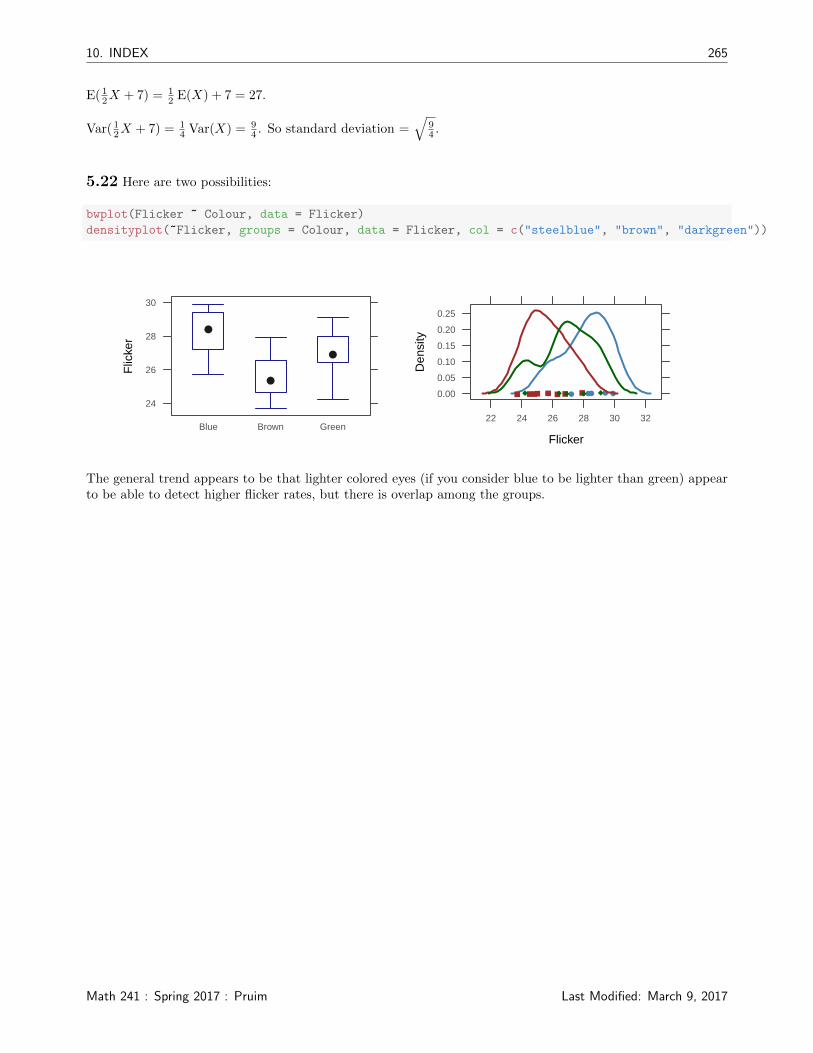
5.22 Here are two possibilities:

bwplot(Flicker ~ Colour, data = Flicker)

densityplot(~Flicker, groups = Colour, data = Flicker, col = c("steelblue", "brown", "darkgreen"))

Flic

ker

24

26

28

30

Blue Brown Green

Flicker

Den

sity

0.00

0.05

0.10

0.15

0.20

0.25

22 24 26 28 30 32

The general trend appears to be that lighter colored eyes (if you consider blue to be lighter than green) appearto be able to detect higher flicker rates, but there is overlap among the groups.


266 10. INDEX

6.1

# 95 % CI

t.star <- qt(0.975, df = 29)

t.star

## [1] 2.045

ME <- t.star * 1.9/sqrt(30)

ME

## [1] 0.7095

1.2 + c(-1, 1) * ME

## [1] 0.4905 1.9095

# 99 % CI

t.star <- qt(0.995, df = 29)

t.star

## [1] 2.756

ME <- t.star * 1.9/sqrt(30)

ME

## [1] 0.9562

10.2 + c(-1, 1) * ME

## [1] 9.244 11.156

# standard uncertainty = SE = s / sqrt(n)

1.9/sqrt(30)

## [1] 0.3469

6.2


10. INDEX 267

# rectangualr: sd = width / sqrt(12) = width / (2 * sqrt(3))

0.4 * 2/sqrt(12)

## [1] 0.2309

0.4/sqrt(3)

## [1] 0.2309

# triangular: sd = width / (2 * sqrt(6))

0.4 * 2/(2 * sqrt(6))

## [1] 0.1633

0.4/sqrt(6)

## [1] 0.1633

The uniform distribution is a more conservative assumption. The trianlge distribution should only be used insituations where errors are more likely to be smaller than larger (with the the specified bounds).

6.3

# rectangular

1e-04/sqrt(3)

## [1] 5.774e-05

# trianglular

1e-04/sqrt(6)

## [1] 4.082e-05

6.4 Let f(R) = πR2. Then ∂f∂R = 2πR, so the uncertainty in the area estimation is

√(2πR)2(0.3)2 = 2πR · 0.3 = 23.562m2 .

We can report the area as 490± 20.

6.5


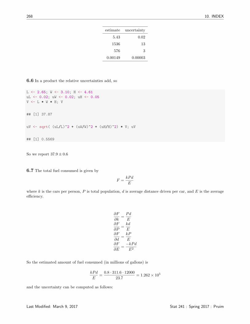
268 10. INDEX

estimate uncertainty

5.43 0.02

1536 13

576 3

0.00149 0.00003

6.6 In a product the relative uncertainties add, so

L <- 2.65; W <- 3.10; H <- 4.61

uL <- 0.02; uW <- 0.02; uH <- 0.05

V <- L * W * H; V

## [1] 37.87

uV <- sqrt( (uL/L)^2 + (uW/W)^2 + (uH/H)^2) * V; uV

## [1] 0.5569

So we report 37.9± 0.6

6.7 The total fuel consumed is given by

F =kPd

E

where k is the cars per person, P is total population, d is average distance driven per car, and E is the averageefficiency.

∂F

∂k=Pd

E∂F

∂P=kd

E∂F

∂d=kP

E∂F

∂E=−kPdE2

So the estimated amount of fuel consumed (in millions of gallons) is

kPd

E=

0.8 · 311.6 · 12000

23.7= 1.262× 105

and the uncertainty can be computed as follows:


10. INDEX 269

k <- 0.8; u_k <- 0.12

P <- 311.6; u_P <- 0.2

d <- 12000; u_d <- 2000

E <- 23.7; u_E <- 1.7

variances <- c(

(P*d/E)^2 * u_k^2 ,

(k*d/E)^2 * u_P^2 ,

(k*P/E)^2 * u_d^2 ,

(k * P * d/E^2)^2 * u_E^2

)

variances

## [1] 358445548 6563 442525367 81967525

u_F <-

sqrt(

(P*d/E)^2 * u_k^2 +

(k*d/E)^2 * u_P^2 +

(k*P/E)^2 * u_d^2 +

(k * P * d/E^2)^2 * u_E^2

)

u_F

## [1] 29714

sqrt(sum(variances))

## [1] 29714

So we might report fuel consumption as 1.3× 105 ± 3× 104 millions of gallons or 130 ± 30 billions of gallons.

Note: This problem can also be done in stages. First we estimate the number of (millions of) cars using

C = kP .

C <- k * P

C

## [1] 249.3

u_C <- sqrt(P^2 * u_k^2 + k^2 * u_P^2)

u_C

## [1] 37.39

The number of (millions of) miles driven is estimated by M = Cd:


270 10. INDEX

M <- C * d

M

## [1] 2991360

u_M <- sqrt(d^2 * u_C^2 + C^2 * u_d^2)

u_M

## [1] 670747

Finally, the fuel used is F = M/E.

F = M/E

u_F = sqrt((1/E)^2 * u_M^2 + (M/E^2)^2 * u_E^2)

u_F

## [1] 29714

This gives the same result (again in millions of gallons of gasoline).

It would also be possible to relative uncertainty to do this problem, since we have nice formulas for the relativeuncertainty in products and quotients.

6.8 See the next problem for the answer.

6.9 Let Q = XY −1. So ∂Q∂X = Y −1 and ∂Q

∂Y = −XY −2. From this we get

uQQ

=

√Y −2u2

X +X2Y −4u2Y

Q2

=

√Y −2u2

X +X2Y −4u2Y

X2Y −2

=

√u2X

X2+u2Y

Y 2

=

√(uXX

)2

+(uYY

)2

which gives a Pythagorean identity for the relative uncertainties just as it did for a product.

V <- 1.637 / 0.43; V

## [1] 3.807

uV <- sqrt( (0.02/.43)^2 + (0.006/1.637)^2 ) * V; uV

## [1] 0.1776

So we report 3.81± 0.18.


10. INDEX 271

7.1

a) The residual degrees of freedom is 13, so there were 13 + 2 = 15 observations.

b) runoff = −1 + 0.83 · rainfall

c) 0.83± 0.04

d) confint(rain.model, "rainfall")

## 2.5 % 97.5 %

## rainfall 0.7481 0.9059

We can compute this from the information displayed:

t.star <- qt( .975, df=13 ) # 13 df listed for residual standard error

t.star

## [1] 2.16

SE <- 0.0365

ME <- t.star * SE; SE

## [1] 0.0365

0.8270 + c(-1,1) * ME # CI as an interval

## [1] 0.7481 0.9059

We should round this using our rounding rules (treating the margin of error like an uncertainty).

e) The slope tells us how much additional run-off there is per additional amount of rain that falls. Sinceboth are in the same units (m3) and since the intercept is essentially 0, we can interpret this slope as aproportion. Roughly 83% of the rain water is being measured as runoff.

f) 5.24

7.2

foot.model <- lm(width ~ length, data = KidsFeet)

plot(foot.model, w = 1)

plot(foot.model, w = 2)


272 10. INDEX

8.5 9.0 9.5

−1.

00.

00.

5

Fitted values

Res

idua

ls

lm(width ~ length)

Residuals vs Fitted

16

3

25

−2 −1 0 1 2

−2

−1

01

2

Theoretical Quantiles

Sta

ndar

dize

d re

sidu

als

lm(width ~ length)

Normal Q−Q

1625

3

Our diagnostics look pretty good. The residuals look randomly distributed with similar amounts of variabilitythroughout the plot. The normal-quantile plot is nearly linear.

f <- makeFun(foot.model)

f(24, interval = "prediction")

## fit lwr upr

## 1 8.813 7.997 9.629

f(24, interval = "confidence")

## fit lwr upr

## 1 8.813 8.666 8.96

We can’t estimate Billy’s foot width very accurately (between 8.0 and 9.6 cm), but we can estimate the averagefoot width for all kids with a foot length of 24 cm more accurately (between 8.67 and 8.96 cm).

7.3


10. INDEX 273

bike.model <- lm(distance ~ space, data = ex12.21)

coef(summary(bike.model))

## Estimate Std. Error t value Pr(>|t|)

## (Intercept) -2.1825 1.05669 -2.065 7.275e-02

## space 0.6603 0.06748 9.786 9.975e-06

f <- makeFun(bike.model)

f(15, interval = "prediction")

## fit lwr upr

## 1 7.723 6.313 9.132

We would use a confidence interval to estimate the average separation distance for all streets with 15 feet ofavailable space.

f(15, interval = "confidence")

## fit lwr upr

## 1 7.723 7.293 8.152

7.4

a) model <- lm(weight ~ height, data = Men)

coef(summary(model))


## (Intercept) -69.6989 12.14450 -5.739 1.551e-08

## height 0.8707 0.06994 12.449 1.277e-31

b) # we can ask for just the parameter we want, if we like

confint(model, parm = "height")

## 2.5 % 97.5 %

## height 0.7333 1.008

The slope tells us how much the average weight (in kg) increases per cm of height.


274 10. INDEX

c) f <- makeFun(model)

# in kg

f(6 * 12 * 2.54, interval = "confidence")

## fit lwr upr

## 1 89.53 87.98 91.09

# in pounds

f(6 * 12 * 2.54, interval = "confidence") * 2.2

## fit lwr upr

## 1 197 193.5 200.4

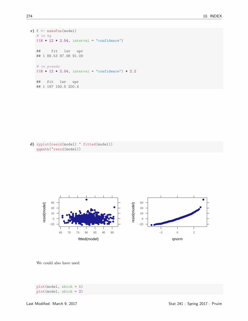
d) xyplot(resid(model) ~ fitted(model))

qqmath(~resid(model))

fitted(model)

resi

d(m

odel

)

−20

0

20

40

60

65 70 75 80 85 90 95

qnorm

resi

d(m

odel

)

−20

0

20

40

60

−2 0 2

We could also have used

plot(model, which = 1)

plot(model, which = 2)


10. INDEX 275

65 75 85 95

−20

2060

Fitted values

Res

idua

ls

lm(weight ~ height)

Residuals vs Fitted

1170

425201

−3 −1 1 2 3

−2

02

46

Theoretical Quantiles

Sta

ndar

dize

d re

sidu

als

lm(weight ~ height)

Normal Q−Q

1170

425201

The residual plot looks fine. There is bit of a bend to the normal-quantile plot, indicating that thedistribution of residuals is a bit skewed (to the right – the heaviest men are farther above the mean weightfor their height than the lightest men are below).

In this particular case, a log transformation of the weights improves the residual distribution. There isstill one man whose weight is quite high for his height, but otherwise things look quite good.

model2 <- lm(log(weight) ~ height, data = Men)

coef(summary(model2))


## (Intercept) 2.51348 0.1448876 17.35 2.146e-54

## height 0.01081 0.0008344 12.95 8.626e-34

xyplot(resid(model2) ~ fitted(model2))

qqmath(~resid(model2))

fitted(model2)

resi

d(m

odel

2)

−0.2

0.0

0.2

0.4

0.6

4.2 4.3 4.4 4.5

qnorm

resi

d(m

odel

2)

−0.2

0.0

0.2

0.4

0.6

−2 0 2

This model says thatlog(weight) = 2.51 + 0.011 · height

Soweight = 12.3 · (1.011)height


p(y g y p(g y - calvin collegerpruim/courses/s241/s17/test-info/test02... ·...

Documents