pysd-cookbook documentation · •to get started learning python, an excellent collection of...
TRANSCRIPT
PySD-Cookbook DocumentationRelease 0.1.0
James Houghton
Mar 08, 2017

Contents
1 Quickstart 3
2 How to use this cookbook 5
3 Contents 73.1 Getting Started . . . . . . . . . . . . . . . . . . . . . . . . . . . . . . . . . . . . . . . . . . . . . . 73.2 Data Handling . . . . . . . . . . . . . . . . . . . . . . . . . . . . . . . . . . . . . . . . . . . . . . 233.3 Visualization . . . . . . . . . . . . . . . . . . . . . . . . . . . . . . . . . . . . . . . . . . . . . . . 303.4 Model Fitting . . . . . . . . . . . . . . . . . . . . . . . . . . . . . . . . . . . . . . . . . . . . . . . 433.5 Geographic Analyses . . . . . . . . . . . . . . . . . . . . . . . . . . . . . . . . . . . . . . . . . . . 593.6 Surrogating Functions . . . . . . . . . . . . . . . . . . . . . . . . . . . . . . . . . . . . . . . . . . 773.7 Realtime Data Incorporation . . . . . . . . . . . . . . . . . . . . . . . . . . . . . . . . . . . . . . . 813.8 Model Development Workflow . . . . . . . . . . . . . . . . . . . . . . . . . . . . . . . . . . . . . 873.9 Data Used in this Cookbook . . . . . . . . . . . . . . . . . . . . . . . . . . . . . . . . . . . . . . . 883.10 Chapters to be Written . . . . . . . . . . . . . . . . . . . . . . . . . . . . . . . . . . . . . . . . . . 983.11 End Notes . . . . . . . . . . . . . . . . . . . . . . . . . . . . . . . . . . . . . . . . . . . . . . . . 99
4 Extra Resources 101
5 Indices and tables 103
i

ii

PySD-Cookbook Documentation, Release 0.1.0
Simple recipes for powerful analysis of system dynamics models
Contents 1

PySD-Cookbook Documentation, Release 0.1.0
2 Contents
CHAPTER 1
Quickstart
1. Download and install Anaconda Python 3.6+
2. Install PySD with pip using the command pip install pysd at your command prompt
3. Download this cookbook and unzip it to a working directory
4. Navigate your command prompt to the working directory just created
5. Launch ipython notebook with the command ipython notebook at your command prompt
6. In the ipython browser, open source\analyses\getting_started\Hello_World_Teacup.ipynb
3

PySD-Cookbook Documentation, Release 0.1.0
4 Chapter 1. Quickstart
CHAPTER 2
How to use this cookbook
Every recipe in this cookbook is an executable ipython notebook. Because of this, I recommend that you downloada copy of the cookbook, and follow along by executing the steps in each notebook as you read, playing with theparameters, etc.
If you want to implement a recipe, you can then make a copy of the notebook you are interested in, and modify it toanalyze your own problem with your own data.
To download the cookbook in its entirity, use this link or visit the cookbook’s Github Page and select one of the optionsin the righthand panel.
5

PySD-Cookbook Documentation, Release 0.1.0
6 Chapter 2. How to use this cookbook
CHAPTER 3
Contents
Getting Started
Introduction to the PySD Cookbook
Dear Reader,
This cookbook is intended to be a resource for system dynamicists interested in applying the power of python analyticsto their simulation models.
Every recipe in this cookbook is an executable Jupyter Notebook (a.k.a. iPython Notebook). Because of this, Irecommend that you download a copy of the cookbook, open the source files and follow along by executing the stepsin each recipe as you read, playing with the parameters, etc. If you want to implement a recipe, you can make a copyof the notebook you are interested in, and modify it to analyze your own problem with your own data.
Workbook versions of many recipes are available for use in a classroom setting. In these workbooks, components ofthe code have been removed for students to fill in on their own. These are identified with a trailing _Workbook inthe filename.
You can download the cookbook as a zip file from this link, or, if you prefer, create a fork of the repository from itsgithub page, and clone it to your computer.
If you come up with an interesting recipe of your own, I’d love to have your contributions. If you find a bug in thescripts used in this cookbook, or have a suggestion for improvements, I’d encourage you to submit an issue on theproject’s issue tracker. If you find a bug in the way PySD itself behaves, the PySD Issue Tracker is a great place toraise it.
Thanks for being interested and supportive of this project. I hope you find the tools presented here to be useful.
Happy Coding!
James Houghton
Installation and Setup of Python and PySD
7
PySD-Cookbook Documentation, Release 0.1.0
Using Anaconda
The simplest way to get started with Python is to use a prepackaged version such as Anaconda from Continuumanalytics.
PySD works with Python 2.7+ or 3.5+. I recommend using the latest version of python 3 from the following link:https://www.continuum.io/downloads
Installing PySD
With a python environment set up, at the command prompt you can type:
pip install pysd
this should install PySD and all of its dependencies. In some cases you may need to prepend the command with ‘sudo’to give it administrative priveledges:
sudo pip install pysd
You’ll be prompted for your administrator password.
Manually installing PySD’s dependencies
On the off chance that pip fails to install the dependencies, you can do the task yourself.
There are a few packages which form the core of the python scientific computing stack. They are:
1. numpy - a library for matrix-type numerical computation
2. scipy - a library which extends numpy with a bunch of useful features, such as stats, etc.
3. matplotlib - a basic plotting library
4. pandas - a basic data manipulation library
5. ipython - an environment for interacting with python and writing clever text/documentation documents, such asthis one.
PySD also requires a few additional package beyond the basic data science stack:
1. parsimonious - a text parsing library
2. yapf - a python code formatting library
To install these packages, use the syntax:
pip install numpy
Run the command once for each package, replacing numpy with scipy, matplotlib, etc.
Launch Jupyter Notebook, and get started
If you used the anaconda graphical installer, you should have a ‘Anaconda Launcher’ user interface installed. Openingthis program and clicking the ‘Jupyter Notebook’ will fire up the notebook explorer in your browser.
Alternately, at your command line type:
8 Chapter 3. Contents
PySD-Cookbook Documentation, Release 0.1.0
jupyter notebook
Your browser should start, and give you a document much like this one that you can play with.
Upgrading PySD
PySD is a work in progress, and from time to time, we’ll ipgrade its features. To upgrade to the latest version of PySD(or any of the other packages, for that matter) use the syntax:
pip install pysd --upgrade
Getting Started with Python
Why should system dynamicists learn to code?
There is a whole world of computational and analysis tools being developed in the larger data science community. Ifsystem dynamicists want to take advantage of these tools, we have two options:
1. we can replicate each of them within one of the system dynamics modeling tools we are familiar with
2. we can bring system dynamics models to the environment where these tools already exist.
PySD and this cookbook are an outgrowth of the belief that this second path is the best use of our time. Bringingthe tools of system dynamics to the wider world of data science allows us to operate within our core competency asmodel builders, and avoids doubled effort. It allows those who are familiar with programming to explore using systemdynamics in their own projects, and ensures that the learning system dynamicists do to use these external tools willhave application in the wider world.
Why Python?
Python is a high-level programming language that allows users to write code quickly and spend less time muckingabout with the boring bits of programming. As a result, it is becoming increasingly popular and is the focus fordevelopment of a wealth of data science tools.
In the pen-strokes of xkcd:
A (very) brief intro to programming in python
Basic Python Data Structures
• Everything in python is an object.
• Objects have different ‘types’.
• Objects can be made up of other objects.
• Variable names are just labels assigned to point to specific objects.
3.1. Getting Started 9
PySD-Cookbook Documentation, Release 0.1.0
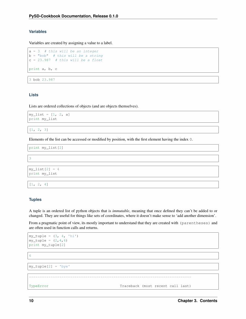
Variables
Variables are created by assigning a value to a label.
a = 3 # this will be an integerb = "bob" # this will be a stringc = 23.987 # this will be a float
print a, b, c
3 bob 23.987
Lists
Lists are ordered collections of objects (and are objects themselves).
my_list = [1, 2, a]print my_list
[1, 2, 3]
Elements of the list can be accessed or modified by position, with the first element having the index 0.
print my_list[2]
3
my_list[2] = 4print my_list
[1, 2, 4]
Tuples
A tuple is an ordered list of python objects that is immutable, meaning that once defined they can’t be added to orchanged. They are useful for things like sets of coordinates, where it doesn’t make sense to ‘add another dimension’.
From a pragmatic point of view, its mostly important to understand that they are created with (parentheses) andare often used in function calls and returns.
my_tuple = (3, 4, 'hi')my_tuple = (2,4,6)print my_tuple[2]
6
my_tuple[2] = 'bye'
---------------------------------------------------------------------------
TypeError Traceback (most recent call last)
10 Chapter 3. Contents
PySD-Cookbook Documentation, Release 0.1.0
<ipython-input-17-5f5c7c118dde> in <module>()----> 1 my_tuple[2] = 'bye'
TypeError: 'tuple' object does not support item assignment
Dictionaries
Dictionaries are named collections of objects which can be accessed by their label:
my_dictionary = {'key 1': 1, 'key 2': b}print my_dictionary['key 2']
bob
You can add elements to a dictionary by assigning to an undefined element
my_dictionary['key 3'] = 27print my_dictionary
{'key 1': 1, 'key 2': 'bob', 'key 3': 27}
Python Control Flow
if statements
The body of an if statement must be indented - standard practice is 4 spaces.
if True:print 'Inside the if statement'
Inside the if statement
if 5 < 3:print 'In the if'
else:if 5 > 3:
print 'in the elif'else:
print 'In the else'
in the elif
if 5 < 3:print 'In the if'
elif 5 >= 3:print 'in the elif'
else:print 'in the else'
3.1. Getting Started 11
PySD-Cookbook Documentation, Release 0.1.0
This runs instead
for loops
For loops allow you to iterate over lists.
my_list = [1, 2, 3, 'bob']
for emile in my_list:print emile
23bob
If we want to iterate over a list of numbers, as is often the case with a for loop, we can use the range function toconstruct the list for us:
for i in range(0, 10):if i > 3:
print i,else:
print 'bob',
bob bob bob bob 4 5 6 7 8 9
Python Functions
Functions are defined using the syntax below. As with if and for, indentation specifies the scope of the function.
def my_function(param1, param2):result = param1 + param2return result
print my_function(3, 4)
7
Functions can have default arguments, making them optional to use in the function call:
def my_other_function(param1=5, param2=10):return param1 * param2
print my_other_function(param2=4)
20
---------------------------------------------------------------------------
NameError Traceback (most recent call last)
<ipython-input-35-1b17a9a8d97e> in <module>()
12 Chapter 3. Contents
PySD-Cookbook Documentation, Release 0.1.0
4 print my_other_function(param2=4)5
----> 6 print param2
NameError: name 'param2' is not defined
Methods and Attributes of Objects
Many python objects have their own methods, which are functions that apply specifically to the object, as in the stringmanipulation functions below:
my_string = 'How about a beer?'print my_string.lower()print my_string.upper().rjust(30) # chained call to methodprint my_string.replace('?', '!')
how about a beer?HOW ABOUT A BEER?
How about a beer!
Some objects have attributes which are not functions that act upon the object, but components of the object’s internalrepresentation.
In the example below, we define a complex number, which has both a real part and a complex part, which we canaccess as an attribute.
my_variable = 12.3 + 4jprint my_variableprint my_variable.realprint my_variable.imag
(12.3+4j)12.34.0
Resources for learning to program using Python.
• To get started learning python, an excellent collection of resources is available in The Hitchhiker’s Guide toPython.
• To try Python in the browser visit learnpython.org.
• Check out this overview of Python for computational statistics
• Online course on python for data science
and finally...
import this
The Zen of Python, by Tim Peters
Beautiful is better than ugly.Explicit is better than implicit.
3.1. Getting Started 13
PySD-Cookbook Documentation, Release 0.1.0
Simple is better than complex.Complex is better than complicated.Flat is better than nested.Sparse is better than dense.Readability counts.Special cases aren't special enough to break the rules.Although practicality beats purity.Errors should never pass silently.Unless explicitly silenced.In the face of ambiguity, refuse the temptation to guess.There should be one-- and preferably only one --obvious way to do it.Although that way may not be obvious at first unless you're Dutch.Now is better than never.Although never is often better than right now.If the implementation is hard to explain, it's a bad idea.If the implementation is easy to explain, it may be a good idea.Namespaces are one honking great idea -- let's do more of those!
Using the Jupyter Notebook
The Jupyter (formerly iPython) Notebook is a browser-based interactive coding environment that allows cells of text(such as this one) to be interspersed with cells of code (such as the next cell), and the output of that code (immediatelyfollowing)
string = 'Hello, World!'print string
Hello, World!
Code Cells
To add cells to the notebook, click the [+] button in the notebook’s tool pane. A new cell will appear below the onewhich is selected. By default this cell is set for writing code snippets.
To execute code in a cell such as this, select it and press either the play [>|] button in the tool pane, or press<shift><enter>. The results of the cell’s computation will be displaced below.
Once a cell has been run, the variables declared in that cell are available to any other cell in the notebook:
print string[:6] + ' Programmer!'
Hello, Programmer!
Text Cells
To format a cell as text, with the desired cell highlighted, click the dropdown in the tool pane showing the word Code,and select Markdown.
Markdown is a simple syntax for formatting text. Headings are indicated with pound signs #:
### Heading
14 Chapter 3. Contents
PySD-Cookbook Documentation, Release 0.1.0
Heading~~~~~~~
Italics and bold are indicated with one and two preceeding and following asterisks respectively: *Italics* : Italics,**Bold** : Bold
Code is blocked with tick fences (same key as tilde, not single quotes):
```Code goes here```
and quotes are preceeded with the right-pointy chevron ‘>‘ > “This is not my quote.” - Benjamin Franklin
Tab-completion
While you’re typing code, it’s often possible to just start the word you want, and hit the <tab> key. iPython will giveyou a list of suggestions for how to complete that term.
For example, in the box below, if you place the cursor after my, ipython will show the above two variable names asoptions, which you can select and enter.
my_very_long_variable_name = 2my_fairly_long_variable_name = 3my
Context help
It is sometimes hard to remember what arguments a function takes (or what order they come in).
If you type the name of the function and the open parenthesis, and then press <shift><tab>, a tooltip will comeup showing you what arguments the function expects.
sum(
References
• A comprehensive tutorial to using the Jupyter Notebook
Working with git and github
git is a version control system used widely by software developers to manage their codebase, as it has excellentsupport for collaboration, allowing different individuals to work on the same codebase, and combine their efforts.
Github is an online service that uses the git version control system to store files and faciliatate collaboration onsoftware projects. The code for PySD is hosted with github, as is that for much of the open source software community.
For system dynamicists, Github is a useful tool for tracking changes to a model or analysis code, documenting the de-velopment process, and facilitating model collaboration. For academics, it can serve as a permanent, citable repositoryfor scripts used to prepare an academic paper, thus facilitating replication and extension of the research.
While the workflow may seem intimidating, once mastered it can prevent a lot of headaches.
3.1. Getting Started 15
PySD-Cookbook Documentation, Release 0.1.0
Resources
Rather than include a tutorial of the github workflow in this cookbook, I’ll point to several resources for getting startedwith git and github:
• Interactive tutorial for using git and github at the command line
• Getting Started with Github video
• Github Desktop GUI Tool
Hello World: The Teacup Model
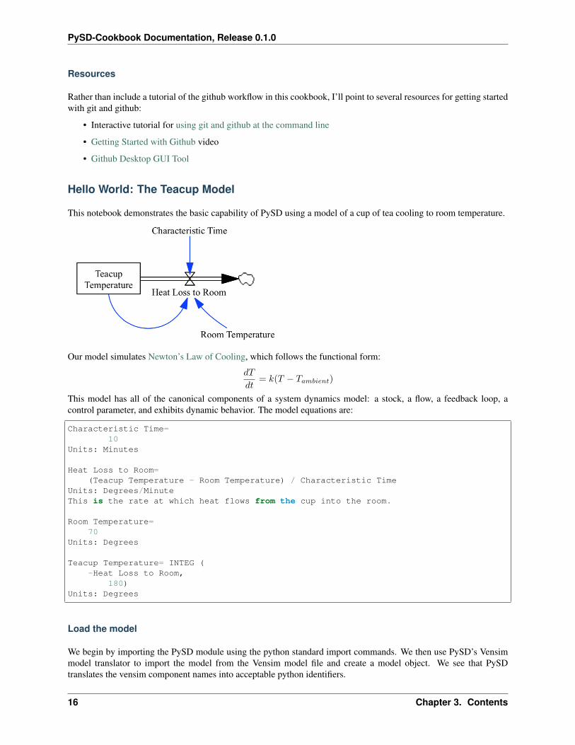
This notebook demonstrates the basic capability of PySD using a model of a cup of tea cooling to room temperature.
Our model simulates Newton’s Law of Cooling, which follows the functional form:
𝑑𝑇
𝑑𝑡= 𝑘(𝑇 − 𝑇𝑎𝑚𝑏𝑖𝑒𝑛𝑡)
This model has all of the canonical components of a system dynamics model: a stock, a flow, a feedback loop, acontrol parameter, and exhibits dynamic behavior. The model equations are:
Characteristic Time=10
Units: Minutes
Heat Loss to Room=(Teacup Temperature - Room Temperature) / Characteristic Time
Units: Degrees/MinuteThis is the rate at which heat flows from the cup into the room.
Room Temperature=70
Units: Degrees
Teacup Temperature= INTEG (-Heat Loss to Room,
180)Units: Degrees
Load the model
We begin by importing the PySD module using the python standard import commands. We then use PySD’s Vensimmodel translator to import the model from the Vensim model file and create a model object. We see that PySDtranslates the vensim component names into acceptable python identifiers.
16 Chapter 3. Contents
PySD-Cookbook Documentation, Release 0.1.0
%pylab inlineimport pysdmodel = pysd.read_vensim('../../models/Teacup/Teacup.mdl')
Populating the interactive namespace from numpy and matplotlib
The read_vensim command we have just run does two things. First it translates the model into a python modulewhich is stored ../../models/Teacup/Teacup.py in the same directory as the original file, with the filenamechanged to .py. You can go and have a look at the file and compare it to the vensim model file that it came from toget a sense for how the translation works.
The second thing the function does is load that translated python file into a PySD object and return it for use.
Run with default parameters
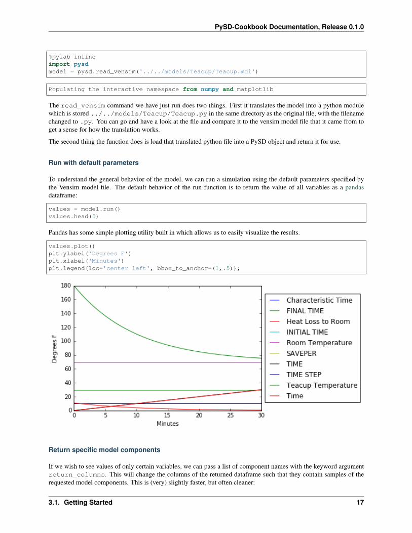
To understand the general behavior of the model, we can run a simulation using the default parameters specified bythe Vensim model file. The default behavior of the run function is to return the value of all variables as a pandasdataframe:
values = model.run()values.head(5)
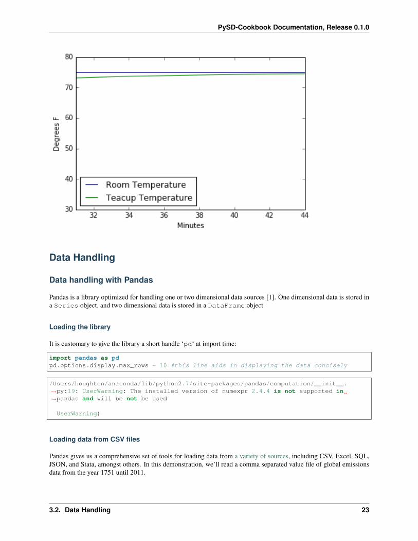
Pandas has some simple plotting utility built in which allows us to easily visualize the results.
values.plot()plt.ylabel('Degrees F')plt.xlabel('Minutes')plt.legend(loc='center left', bbox_to_anchor=(1,.5));
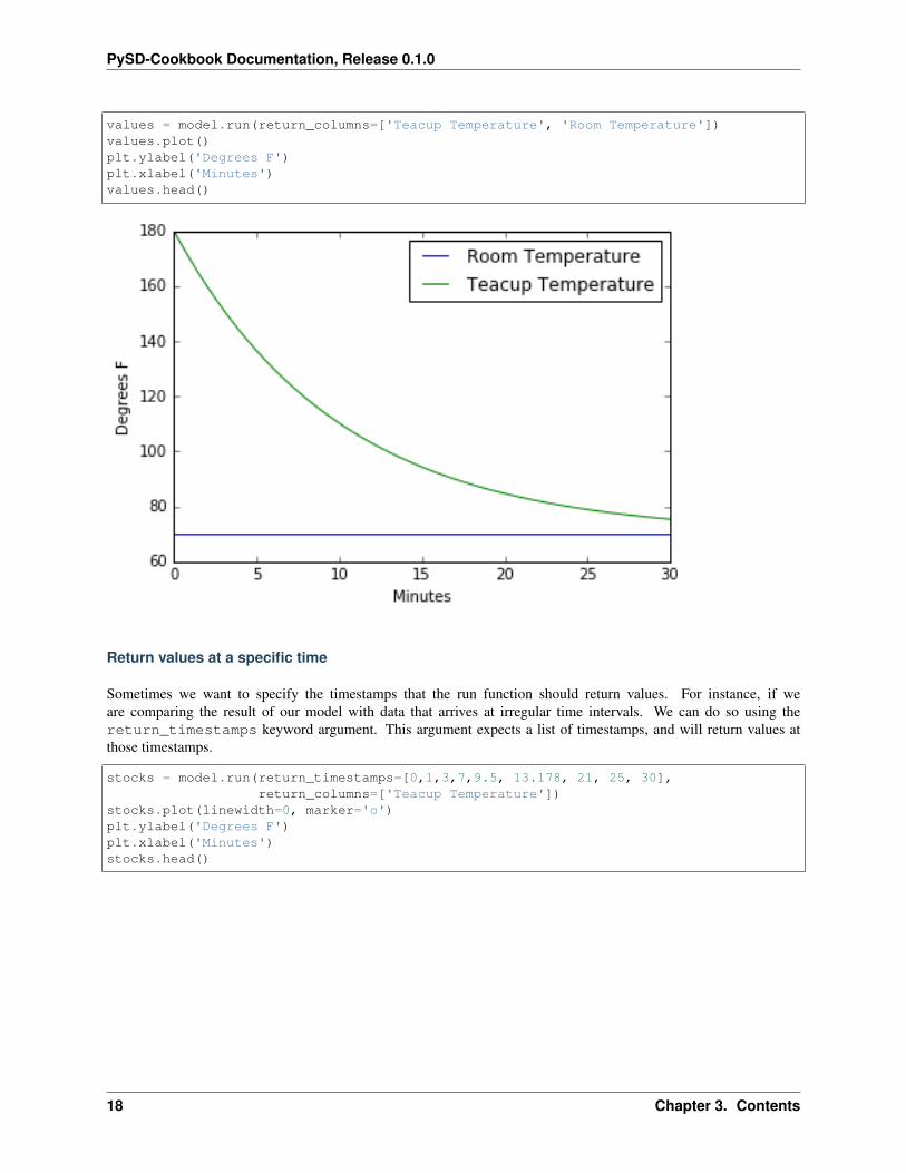
Return specific model components
If we wish to see values of only certain variables, we can pass a list of component names with the keyword argumentreturn_columns. This will change the columns of the returned dataframe such that they contain samples of therequested model components. This is (very) slightly faster, but often cleaner:
3.1. Getting Started 17
PySD-Cookbook Documentation, Release 0.1.0
values = model.run(return_columns=['Teacup Temperature', 'Room Temperature'])values.plot()plt.ylabel('Degrees F')plt.xlabel('Minutes')values.head()
Return values at a specific time
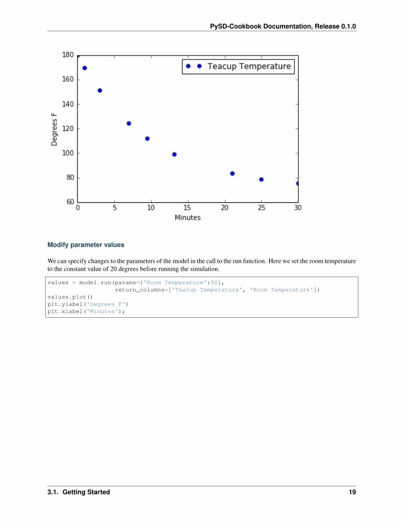
Sometimes we want to specify the timestamps that the run function should return values. For instance, if weare comparing the result of our model with data that arrives at irregular time intervals. We can do so using thereturn_timestamps keyword argument. This argument expects a list of timestamps, and will return values atthose timestamps.
stocks = model.run(return_timestamps=[0,1,3,7,9.5, 13.178, 21, 25, 30],return_columns=['Teacup Temperature'])
stocks.plot(linewidth=0, marker='o')plt.ylabel('Degrees F')plt.xlabel('Minutes')stocks.head()
18 Chapter 3. Contents
PySD-Cookbook Documentation, Release 0.1.0
Modify parameter values
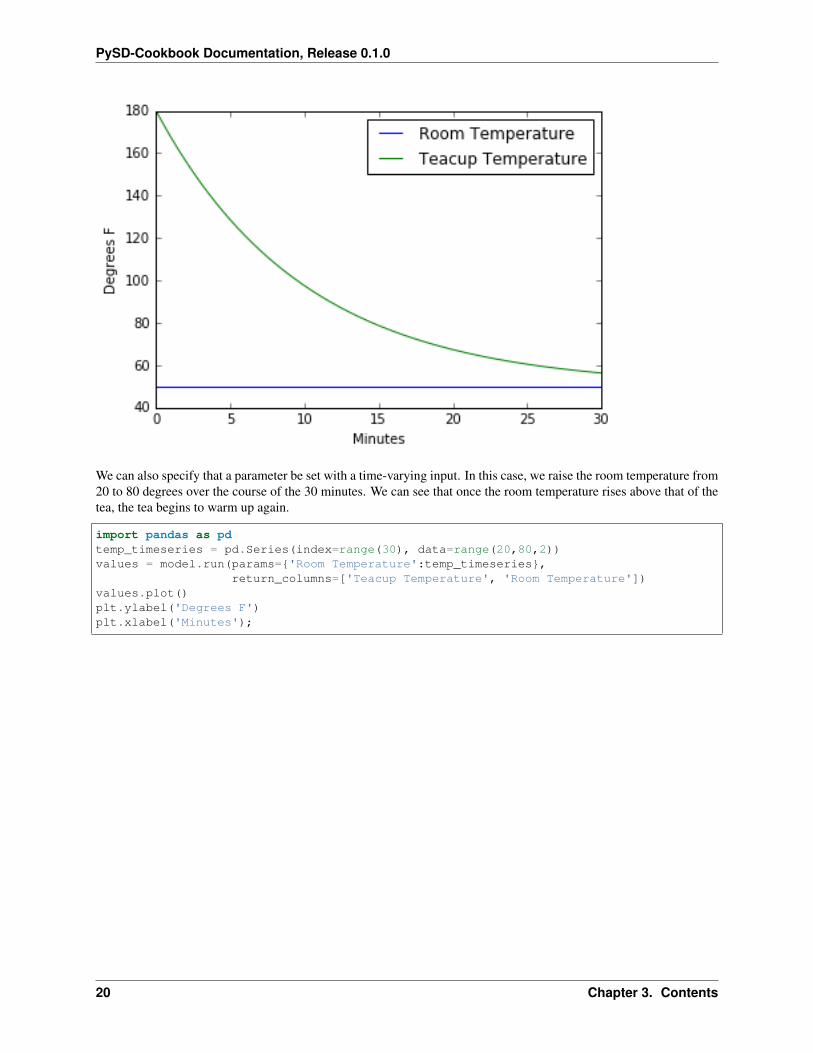
We can specify changes to the parameters of the model in the call to the run function. Here we set the room temperatureto the constant value of 20 degrees before running the simulation.
values = model.run(params={'Room Temperature':50},return_columns=['Teacup Temperature', 'Room Temperature'])
values.plot()plt.ylabel('Degrees F')plt.xlabel('Minutes');
3.1. Getting Started 19
PySD-Cookbook Documentation, Release 0.1.0
We can also specify that a parameter be set with a time-varying input. In this case, we raise the room temperature from20 to 80 degrees over the course of the 30 minutes. We can see that once the room temperature rises above that of thetea, the tea begins to warm up again.
import pandas as pdtemp_timeseries = pd.Series(index=range(30), data=range(20,80,2))values = model.run(params={'Room Temperature':temp_timeseries},
return_columns=['Teacup Temperature', 'Room Temperature'])values.plot()plt.ylabel('Degrees F')plt.xlabel('Minutes');
20 Chapter 3. Contents
PySD-Cookbook Documentation, Release 0.1.0
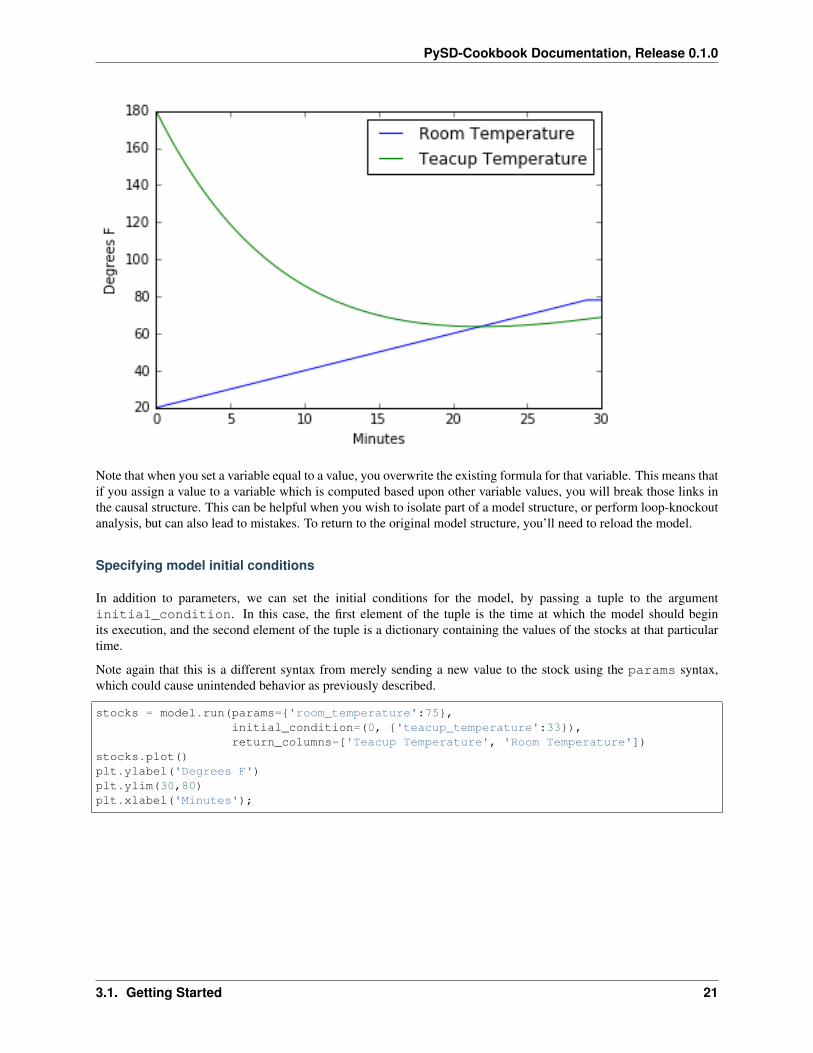
Note that when you set a variable equal to a value, you overwrite the existing formula for that variable. This means thatif you assign a value to a variable which is computed based upon other variable values, you will break those links inthe causal structure. This can be helpful when you wish to isolate part of a model structure, or perform loop-knockoutanalysis, but can also lead to mistakes. To return to the original model structure, you’ll need to reload the model.
Specifying model initial conditions
In addition to parameters, we can set the initial conditions for the model, by passing a tuple to the argumentinitial_condition. In this case, the first element of the tuple is the time at which the model should beginits execution, and the second element of the tuple is a dictionary containing the values of the stocks at that particulartime.
Note again that this is a different syntax from merely sending a new value to the stock using the params syntax,which could cause unintended behavior as previously described.
stocks = model.run(params={'room_temperature':75},initial_condition=(0, {'teacup_temperature':33}),return_columns=['Teacup Temperature', 'Room Temperature'])
stocks.plot()plt.ylabel('Degrees F')plt.ylim(30,80)plt.xlabel('Minutes');
3.1. Getting Started 21
PySD-Cookbook Documentation, Release 0.1.0
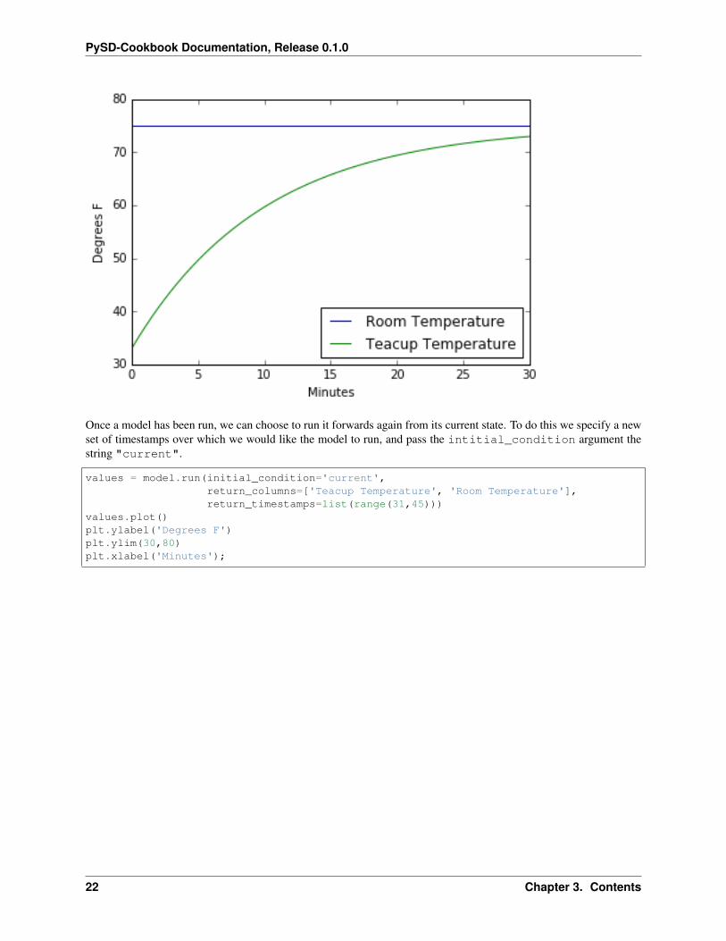
Once a model has been run, we can choose to run it forwards again from its current state. To do this we specify a newset of timestamps over which we would like the model to run, and pass the intitial_condition argument thestring "current".
values = model.run(initial_condition='current',return_columns=['Teacup Temperature', 'Room Temperature'],return_timestamps=list(range(31,45)))
values.plot()plt.ylabel('Degrees F')plt.ylim(30,80)plt.xlabel('Minutes');
22 Chapter 3. Contents
PySD-Cookbook Documentation, Release 0.1.0
Data Handling
Data handling with Pandas
Pandas is a library optimized for handling one or two dimensional data sources [1]. One dimensional data is stored ina Series object, and two dimensional data is stored in a DataFrame object.
Loading the library
It is customary to give the library a short handle ‘pd‘ at import time:
import pandas as pdpd.options.display.max_rows = 10 #this line aids in displaying the data concisely
/Users/houghton/anaconda/lib/python2.7/site-packages/pandas/computation/__init__.→˓py:19: UserWarning: The installed version of numexpr 2.4.4 is not supported in→˓pandas and will be not be used
UserWarning)
Loading data from CSV files
Pandas gives us a comprehensive set of tools for loading data from a variety of sources, including CSV, Excel, SQL,JSON, and Stata, amongst others. In this demonstration, we’ll read a comma separated value file of global emissionsdata from the year 1751 until 2011.
3.2. Data Handling 23
PySD-Cookbook Documentation, Release 0.1.0
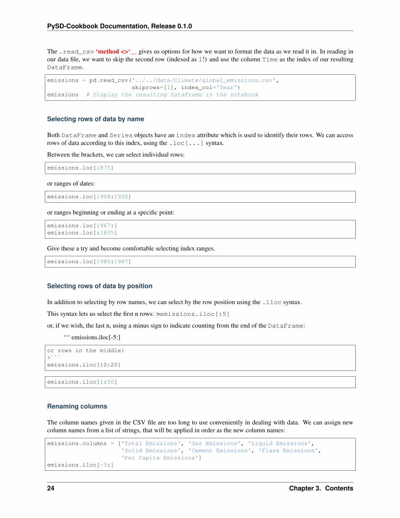
The .read_csv ‘method <>‘__ gives us options for how we want to format the data as we read it in. In reading inour data file, we want to skip the second row (indexed as 1!) and use the column Time as the index of our resultingDataFrame.
emissions = pd.read_csv('../../data/Climate/global_emissions.csv',skiprows=[1], index_col='Year')
emissions # Display the resulting DataFrame in the notebook
Selecting rows of data by name
Both DataFrame and Series objects have an index attribute which is used to identify their rows. We can accessrows of data according to this index, using the .loc[...] syntax.
Between the brackets, we can select individual rows:
emissions.loc[1875]
or ranges of dates:
emissions.loc[1908:1920]
or ranges beginning or ending at a specific point:
emissions.loc[1967:]emissions.loc[:1805]
Give these a try and become comfortable selecting index ranges.
emissions.loc[1985:1987]
Selecting rows of data by position
In addition to selecting by row names, we can select by the row position using the .iloc syntax.
This syntax lets us select the first n rows: >emissions.iloc[:5]
or, if we wish, the last n, using a minus sign to indicate counting from the end of the DataFrame:
‘‘‘ emissions.iloc[-5:]
or rows in the middle:>```emissions.iloc[10:20]
emissions.iloc[1:30]
Renaming columns
The column names given in the CSV file are too long to use conveniently in dealing with data. We can assign newcolumn names from a list of strings, that will be applied in order as the new column names:
emissions.columns = ['Total Emissions', 'Gas Emissions', 'Liquid Emissions','Solid Emissions', 'Cement Emissions', 'Flare Emissions','Per Capita Emissions']
emissions.iloc[-3:]
24 Chapter 3. Contents
PySD-Cookbook Documentation, Release 0.1.0
Accessing specific columns
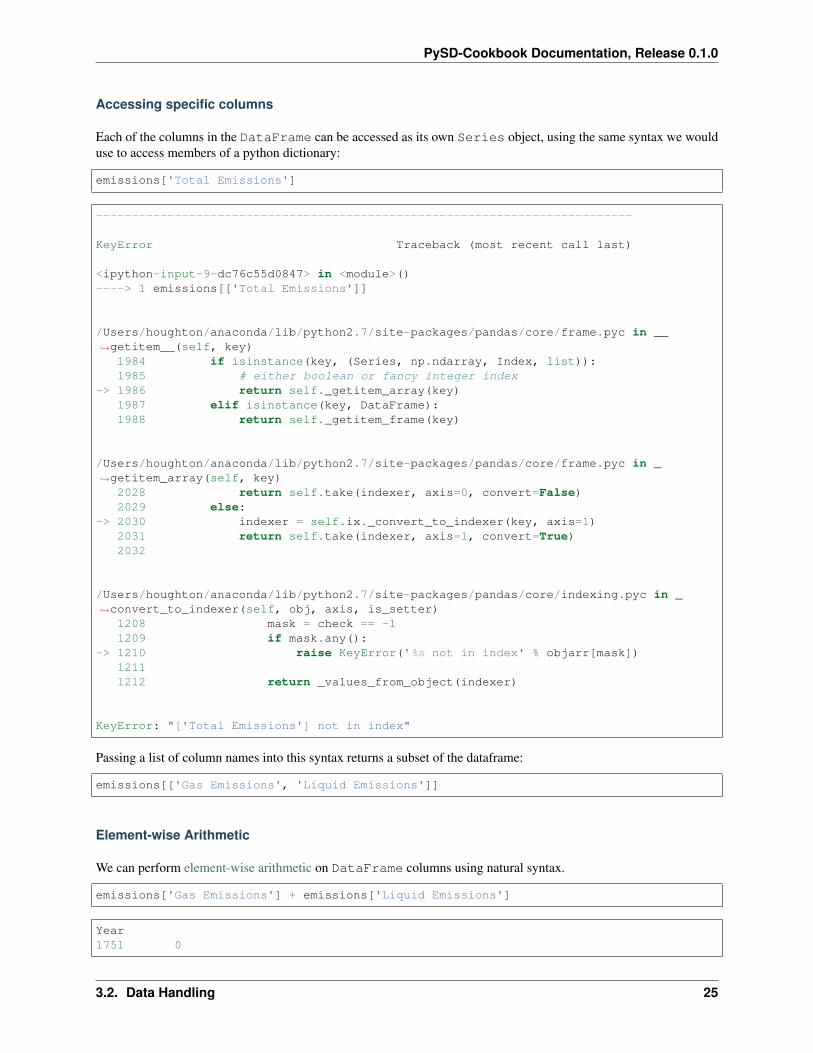
Each of the columns in the DataFrame can be accessed as its own Series object, using the same syntax we woulduse to access members of a python dictionary:
emissions['Total Emissions']
---------------------------------------------------------------------------
KeyError Traceback (most recent call last)
<ipython-input-9-dc76c55d0847> in <module>()----> 1 emissions[['Total Emissions']]
/Users/houghton/anaconda/lib/python2.7/site-packages/pandas/core/frame.pyc in __→˓getitem__(self, key)
1984 if isinstance(key, (Series, np.ndarray, Index, list)):1985 # either boolean or fancy integer index
-> 1986 return self._getitem_array(key)1987 elif isinstance(key, DataFrame):1988 return self._getitem_frame(key)
/Users/houghton/anaconda/lib/python2.7/site-packages/pandas/core/frame.pyc in _→˓getitem_array(self, key)
2028 return self.take(indexer, axis=0, convert=False)2029 else:
-> 2030 indexer = self.ix._convert_to_indexer(key, axis=1)2031 return self.take(indexer, axis=1, convert=True)2032
/Users/houghton/anaconda/lib/python2.7/site-packages/pandas/core/indexing.pyc in _→˓convert_to_indexer(self, obj, axis, is_setter)
1208 mask = check == -11209 if mask.any():
-> 1210 raise KeyError('%s not in index' % objarr[mask])12111212 return _values_from_object(indexer)
KeyError: "['Total Emissions'] not in index"
Passing a list of column names into this syntax returns a subset of the dataframe:
emissions[['Gas Emissions', 'Liquid Emissions']]
Element-wise Arithmetic
We can perform element-wise arithmetic on DataFrame columns using natural syntax.
emissions['Gas Emissions'] + emissions['Liquid Emissions']
Year1751 0
3.2. Data Handling 25
PySD-Cookbook Documentation, Release 0.1.0
1752 01753 01754 01755 0
...2007 46432008 47322009 46212010 47982011 4897dtype: int64
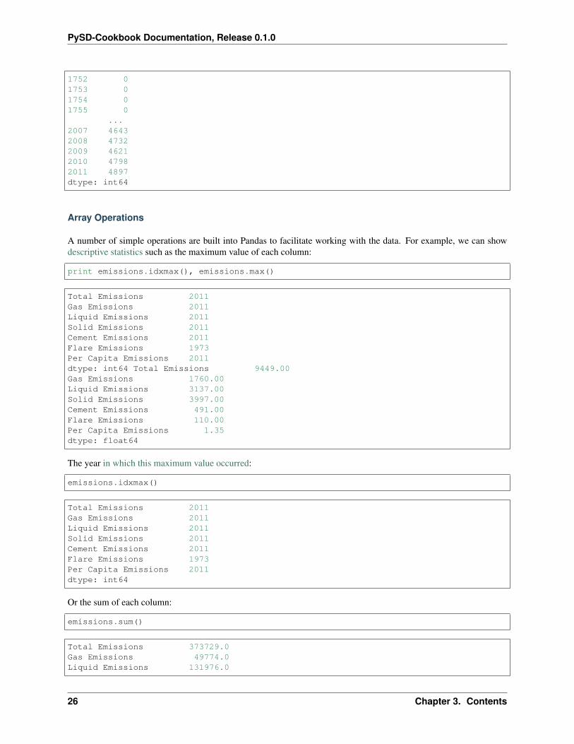
Array Operations
A number of simple operations are built into Pandas to facilitate working with the data. For example, we can showdescriptive statistics such as the maximum value of each column:
print emissions.idxmax(), emissions.max()
Total Emissions 2011Gas Emissions 2011Liquid Emissions 2011Solid Emissions 2011Cement Emissions 2011Flare Emissions 1973Per Capita Emissions 2011dtype: int64 Total Emissions 9449.00Gas Emissions 1760.00Liquid Emissions 3137.00Solid Emissions 3997.00Cement Emissions 491.00Flare Emissions 110.00Per Capita Emissions 1.35dtype: float64
The year in which this maximum value occurred:
emissions.idxmax()
Total Emissions 2011Gas Emissions 2011Liquid Emissions 2011Solid Emissions 2011Cement Emissions 2011Flare Emissions 1973Per Capita Emissions 2011dtype: int64
Or the sum of each column:
emissions.sum()
Total Emissions 373729.0Gas Emissions 49774.0Liquid Emissions 131976.0
26 Chapter 3. Contents
PySD-Cookbook Documentation, Release 0.1.0
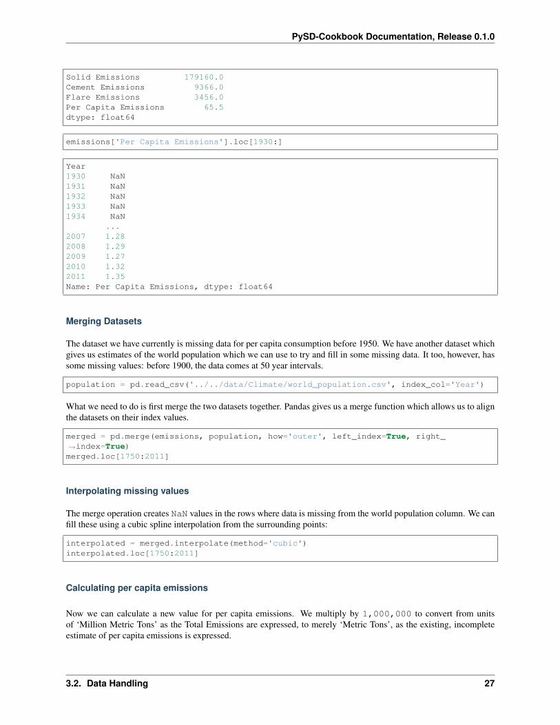
Solid Emissions 179160.0Cement Emissions 9366.0Flare Emissions 3456.0Per Capita Emissions 65.5dtype: float64
emissions['Per Capita Emissions'].loc[1930:]
Year1930 NaN1931 NaN1932 NaN1933 NaN1934 NaN
...2007 1.282008 1.292009 1.272010 1.322011 1.35Name: Per Capita Emissions, dtype: float64
Merging Datasets
The dataset we have currently is missing data for per capita consumption before 1950. We have another dataset whichgives us estimates of the world population which we can use to try and fill in some missing data. It too, however, hassome missing values: before 1900, the data comes at 50 year intervals.
population = pd.read_csv('../../data/Climate/world_population.csv', index_col='Year')
What we need to do is first merge the two datasets together. Pandas gives us a merge function which allows us to alignthe datasets on their index values.
merged = pd.merge(emissions, population, how='outer', left_index=True, right_→˓index=True)merged.loc[1750:2011]
Interpolating missing values
The merge operation creates NaN values in the rows where data is missing from the world population column. We canfill these using a cubic spline interpolation from the surrounding points:
interpolated = merged.interpolate(method='cubic')interpolated.loc[1750:2011]
Calculating per capita emissions
Now we can calculate a new value for per capita emissions. We multiply by 1,000,000 to convert from unitsof ‘Million Metric Tons’ as the Total Emissions are expressed, to merely ‘Metric Tons’, as the existing, incompleteestimate of per capita emissions is expressed.
3.2. Data Handling 27
PySD-Cookbook Documentation, Release 0.1.0
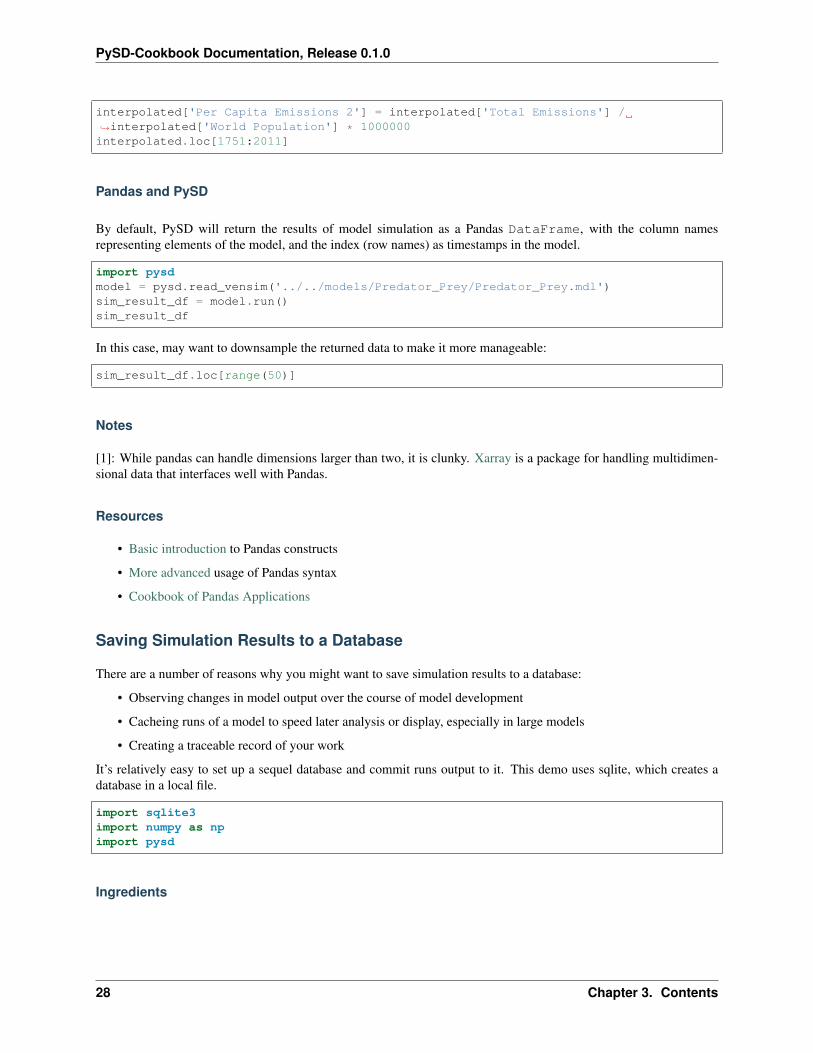
interpolated['Per Capita Emissions 2'] = interpolated['Total Emissions'] /→˓interpolated['World Population'] * 1000000interpolated.loc[1751:2011]
Pandas and PySD
By default, PySD will return the results of model simulation as a Pandas DataFrame, with the column namesrepresenting elements of the model, and the index (row names) as timestamps in the model.
import pysdmodel = pysd.read_vensim('../../models/Predator_Prey/Predator_Prey.mdl')sim_result_df = model.run()sim_result_df
In this case, may want to downsample the returned data to make it more manageable:
sim_result_df.loc[range(50)]
Notes
[1]: While pandas can handle dimensions larger than two, it is clunky. Xarray is a package for handling multidimen-sional data that interfaces well with Pandas.
Resources
• Basic introduction to Pandas constructs
• More advanced usage of Pandas syntax
• Cookbook of Pandas Applications
Saving Simulation Results to a Database
There are a number of reasons why you might want to save simulation results to a database:
• Observing changes in model output over the course of model development
• Cacheing runs of a model to speed later analysis or display, especially in large models
• Creating a traceable record of your work
It’s relatively easy to set up a sequel database and commit runs output to it. This demo uses sqlite, which creates adatabase in a local file.
import sqlite3import numpy as npimport pysd
Ingredients
28 Chapter 3. Contents
PySD-Cookbook Documentation, Release 0.1.0
Model
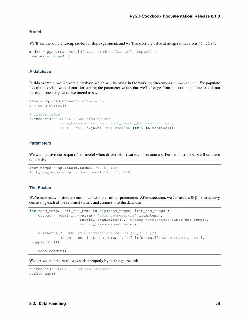
We’ll use the simple teacup model for this experiment, and we’ll ask for the value at integer times from [0..29].
model = pysd.read_vensim('../../models/Teacup/Teacup.mdl')tseries = range(30)
A database
In this example, we’ll create a database which will be saved in the working directory as example.db. We populateits columns with two columns for storing the parameter values that we’ll change from run to run, and then a columnfor each timestamp value we intend to save:
conn = sqlite3.connect('example.db')c = conn.cursor()
# Create tablec.execute('''CREATE TABLE simulations
(room_temperature real, init_teacup_temperature real,%s ) '''%', '.join(['t%i real'%i for i in tseries]));
Parameters
We want to save the output of our model when driven with a variety of parameters. For demonstration, we’ll set theserandomly:
room_temps = np.random.normal(75, 5, 100)init_tea_temps = np.random.normal(175, 15, 100)
The Recipe
We’re now ready to simulate our model with the various parameters. After execution, we construct a SQL insert querrycontaining each of the returned values, and commit it to the database.
for room_temp, init_tea_temp in zip(room_temps, init_tea_temps):output = model.run(params={'room_temperature':room_temp},
initial_condition=(0,{'teacup_temperature':init_tea_temp}),return_timestamps=tseries)
c.execute("INSERT INTO simulations VALUES (%i,%i,%s)"%(room_temp, init_tea_temp, ', '.join(output['teacup_temperature'].
→˓apply(str))))
conn.commit()
We can see that the result was added properly by fetching a record:
c.execute('SELECT * FROM simulations')c.fetchone()
3.2. Data Handling 29
PySD-Cookbook Documentation, Release 0.1.0
(76.0,164.0,164.722280167,156.282130733,148.64516467,141.734949777,135.482334802,129.824731228,124.705520938,120.073467412,115.882212071,112.089807732,108.658298586,105.55333885,102.74385565,100.201730758,97.9015209724,95.8202050685,93.9369526016,92.232915272,90.69103831,89.2958904907,88.0335085264,86.8912580882,85.8577072325,84.9225116976,84.0763117951,83.310638529,82.6178286757,81.9909483832,81.4237236618,80.9104773994)
Finally, we must remember to close our connection to the database:
conn.close()
#remove the database file when we are finished with it.!rm example.db
Visualization
Basic Visualization with matplotlib
Python’s most commonly used plotting library is matplotlib. The library has an interface which mirrors that of Math-works’ Matlab software, and so those with matlab familiarity will find themselves already high up on the learningcurve.
Loading matplotlib and setting up the notebook environment
The matplotlib plotting library has a magic connection with the iPython shell and the notebook environment that allowsstatic images of plots to be rendered in the notebook. Instead of using the normal import ... syntax, we’ll use thisiPython ‘magic’ to not only import the library, but set up the environment we’ll need to create plots.
30 Chapter 3. Contents
PySD-Cookbook Documentation, Release 0.1.0
%pylab inline
Populating the interactive namespace from numpy and matplotlib
Load data to plot
We’ll use the emissions data we saw before in the Pandas tutorial, as it’s familiar:
import pandas as pdemissions = pd.read_csv('../../data/Climate/global_emissions.csv',
skiprows=2, index_col='Year',names=['Year', 'Total Emissions',
'Gas Emissions', 'Liquid Emissions','Solid Emissions', 'Cement Emissions','Flare Emissions', 'Per Capita Emissions'])
emissions.head(3)
/Users/houghton/anaconda/lib/python2.7/site-packages/pandas/computation/__init__.→˓py:19: UserWarning: The installed version of numexpr 2.4.4 is not supported in→˓pandas and will be not be used
UserWarning)
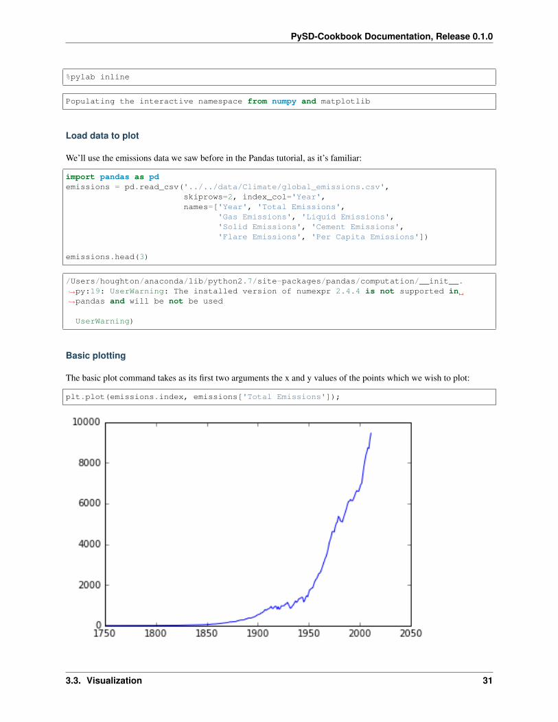
Basic plotting
The basic plot command takes as its first two arguments the x and y values of the points which we wish to plot:
plt.plot(emissions.index, emissions['Total Emissions']);
3.3. Visualization 31
PySD-Cookbook Documentation, Release 0.1.0
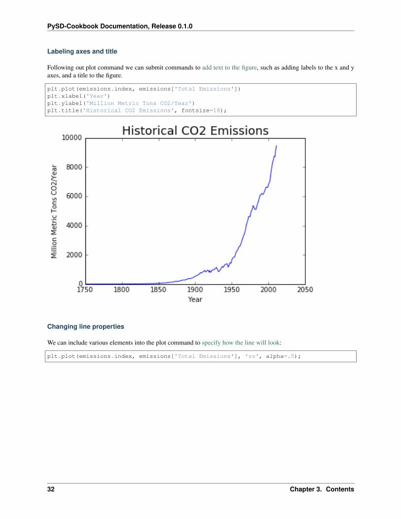
Labeling axes and title
Following out plot command we can submit commands to add text to the figure, such as adding labels to the x and yaxes, and a title to the figure.
plt.plot(emissions.index, emissions['Total Emissions'])plt.xlabel('Year')plt.ylabel('Million Metric Tons CO2/Year')plt.title('Historical CO2 Emissions', fontsize=18);
Changing line properties
We can include various elements into the plot command to specify how the line will look:
plt.plot(emissions.index, emissions['Total Emissions'], 'ro', alpha=.5);
32 Chapter 3. Contents
PySD-Cookbook Documentation, Release 0.1.0
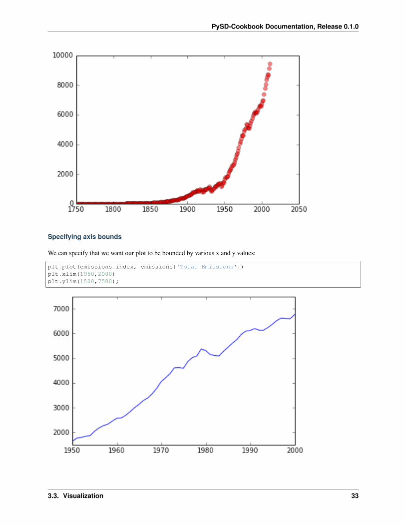
Specifying axis bounds
We can specify that we want our plot to be bounded by various x and y values:
plt.plot(emissions.index, emissions['Total Emissions'])plt.xlim(1950,2000)plt.ylim(1500,7500);
3.3. Visualization 33
PySD-Cookbook Documentation, Release 0.1.0
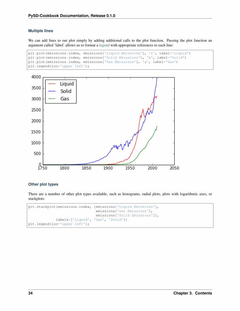
Multiple lines
We can add lines to our plot simply by adding additional calls to the plot function. Passing the plot function anargument called ‘label’ allows us to format a legend with appropriate references to each line:
plt.plot(emissions.index, emissions['Liquid Emissions'], 'r', label='Liquid')plt.plot(emissions.index, emissions['Solid Emissions'], 'b', label='Solid')plt.plot(emissions.index, emissions['Gas Emissions'], 'g', label='Gas')plt.legend(loc='upper left');
Other plot types
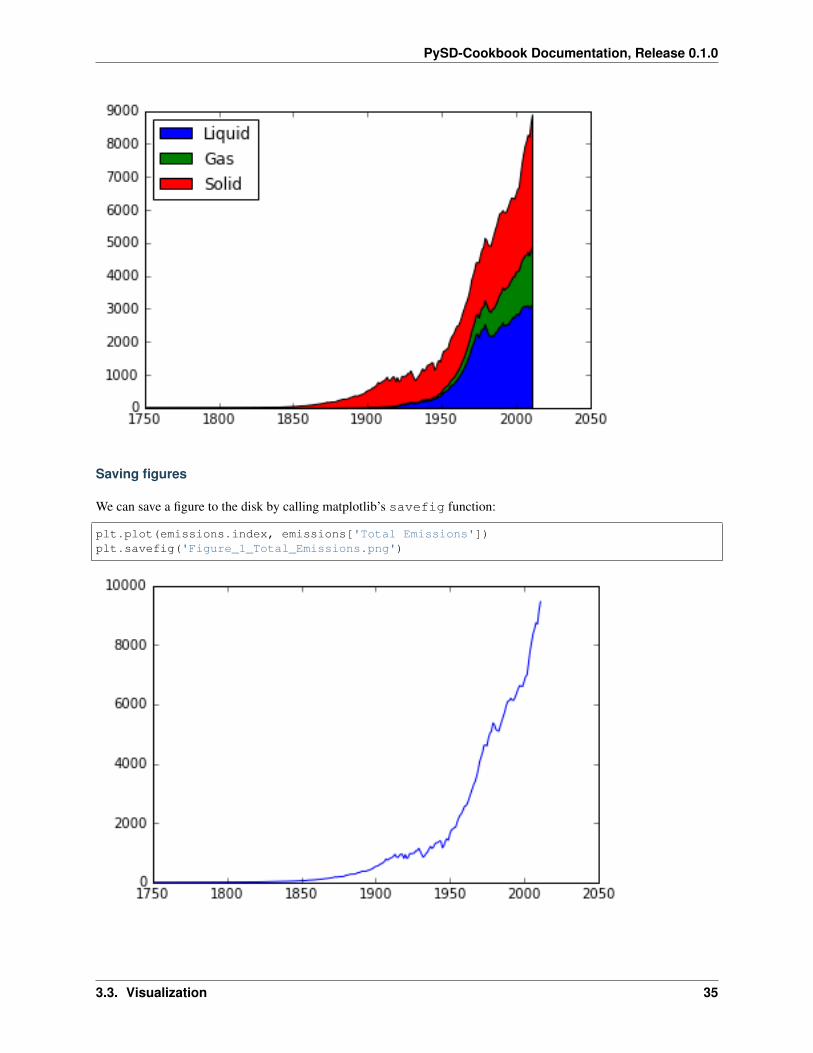
There are a number of other plot types available, such as histograms, radial plots, plots with logarithmic axes, orstackplots:
plt.stackplot(emissions.index, [emissions['Liquid Emissions'],emissions['Gas Emissions'],emissions['Solid Emissions']],
labels=['Liquid', 'Gas', 'Solid'])plt.legend(loc='upper left');
34 Chapter 3. Contents
PySD-Cookbook Documentation, Release 0.1.0
Saving figures
We can save a figure to the disk by calling matplotlib’s savefig function:
plt.plot(emissions.index, emissions['Total Emissions'])plt.savefig('Figure_1_Total_Emissions.png')
3.3. Visualization 35
PySD-Cookbook Documentation, Release 0.1.0
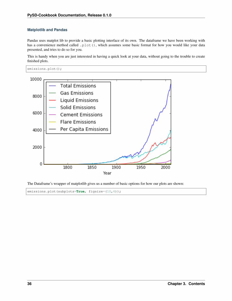
Matplotlib and Pandas
Pandas uses matplot lib to provide a basic plotting interface of its own. The dataframe we have been working withhas a convenience method called .plot(), which assumes some basic format for how you would like your datapresented, and tries to do so for you.
This is handy when you are just interested in having a quick look at your data, without going to the trouble to createfinished plots.
emissions.plot();
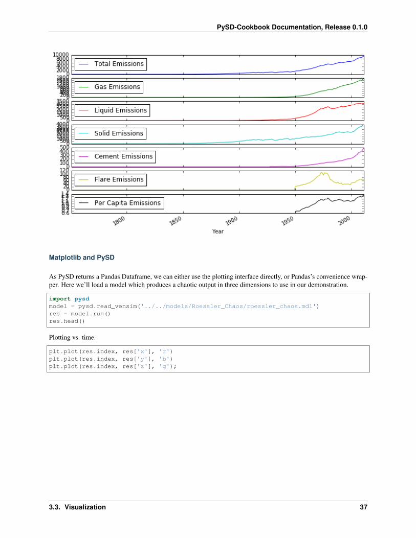
The Dataframe’s wrapper of matplotlib gives us a number of basic options for how our plots are shown:
emissions.plot(subplots=True, figsize=(10,6));
36 Chapter 3. Contents
PySD-Cookbook Documentation, Release 0.1.0
Matplotlib and PySD
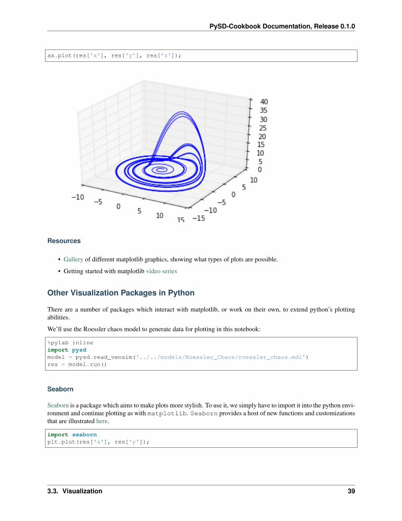
As PySD returns a Pandas Dataframe, we can either use the plotting interface directly, or Pandas’s convenience wrap-per. Here we’ll load a model which produces a chaotic output in three dimensions to use in our demonstration.
import pysdmodel = pysd.read_vensim('../../models/Roessler_Chaos/roessler_chaos.mdl')res = model.run()res.head()
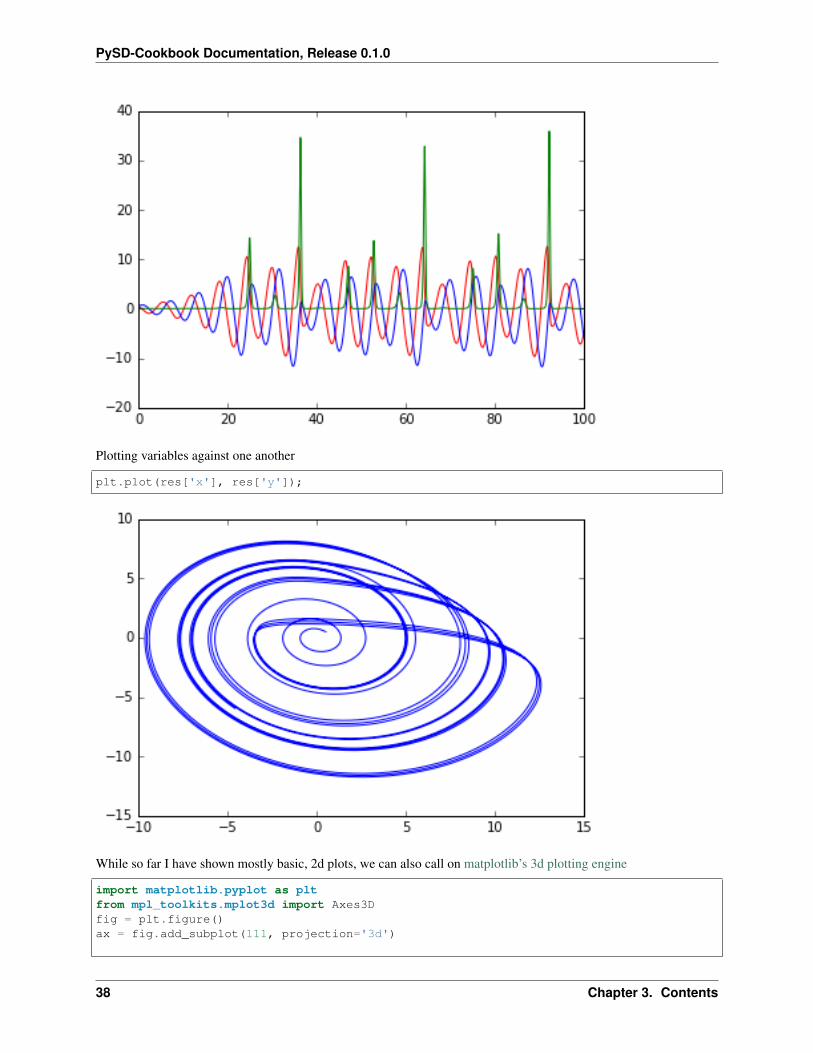
Plotting vs. time.
plt.plot(res.index, res['x'], 'r')plt.plot(res.index, res['y'], 'b')plt.plot(res.index, res['z'], 'g');
3.3. Visualization 37
PySD-Cookbook Documentation, Release 0.1.0
Plotting variables against one another
plt.plot(res['x'], res['y']);
While so far I have shown mostly basic, 2d plots, we can also call on matplotlib’s 3d plotting engine
import matplotlib.pyplot as pltfrom mpl_toolkits.mplot3d import Axes3Dfig = plt.figure()ax = fig.add_subplot(111, projection='3d')
38 Chapter 3. Contents
PySD-Cookbook Documentation, Release 0.1.0
ax.plot(res['x'], res['y'], res['z']);
Resources
• Gallery of different matplotlib graphics, showing what types of plots are possible.
• Getting started with matplotlib video series
Other Visualization Packages in Python
There are a number of packages which interact with matplotlib, or work on their own, to extend python’s plottingabilities.
We’ll use the Roessler chaos model to generate data for plotting in this notebook:
%pylab inlineimport pysdmodel = pysd.read_vensim('../../models/Roessler_Chaos/roessler_chaos.mdl')res = model.run()
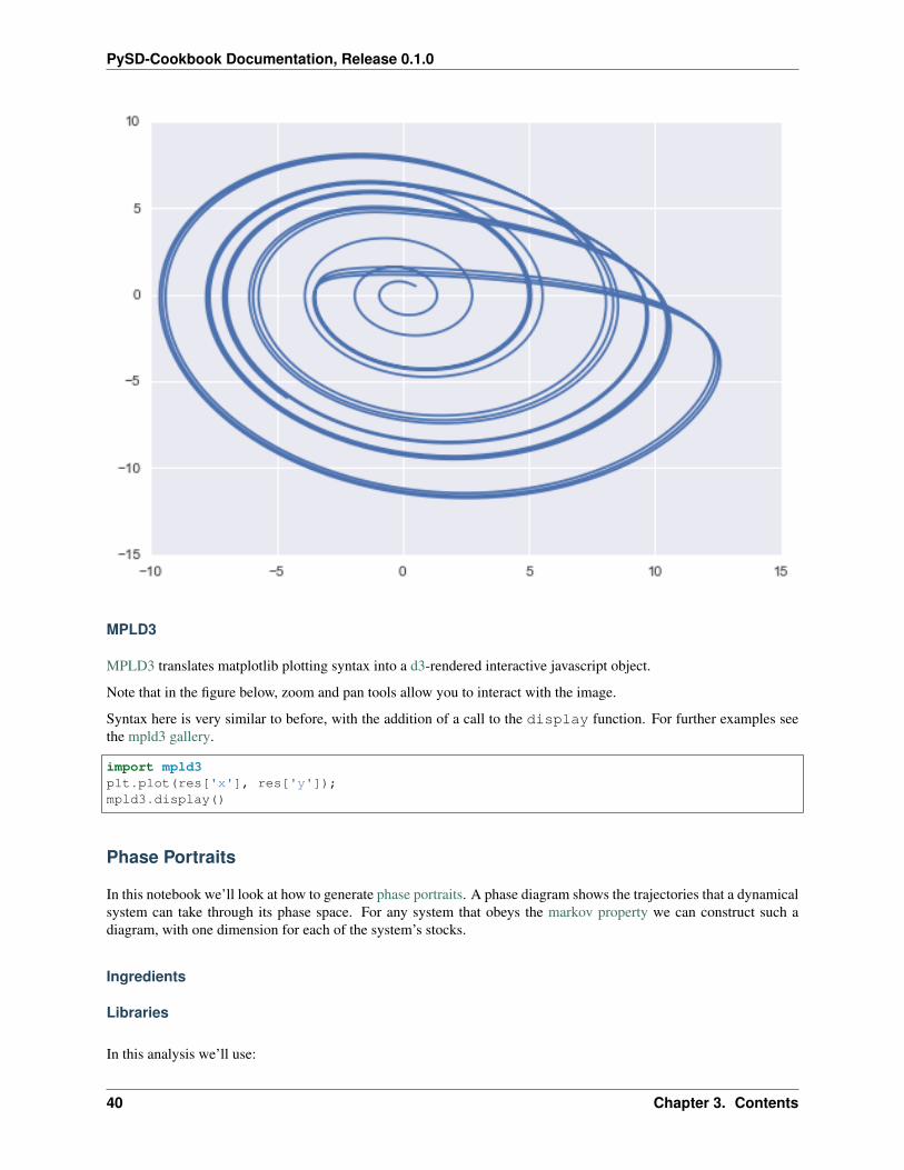
Seaborn
Seaborn is a package which aims to make plots more stylish. To use it, we simply have to import it into the python envi-ronment and continue plotting as with matplotlib. Seaborn provides a host of new functions and customizationsthat are illustrated here.
import seabornplt.plot(res['x'], res['y']);
3.3. Visualization 39
PySD-Cookbook Documentation, Release 0.1.0
MPLD3
MPLD3 translates matplotlib plotting syntax into a d3-rendered interactive javascript object.
Note that in the figure below, zoom and pan tools allow you to interact with the image.
Syntax here is very similar to before, with the addition of a call to the display function. For further examples seethe mpld3 gallery.
import mpld3plt.plot(res['x'], res['y']);mpld3.display()
Phase Portraits
In this notebook we’ll look at how to generate phase portraits. A phase diagram shows the trajectories that a dynamicalsystem can take through its phase space. For any system that obeys the markov property we can construct such adiagram, with one dimension for each of the system’s stocks.
Ingredients
Libraries
In this analysis we’ll use:
40 Chapter 3. Contents
PySD-Cookbook Documentation, Release 0.1.0
• numpy to create the grid of points that we’ll sample over
• matplotlib via ipython’s pylab magic to construct the quiver plot
%pylab inlineimport pysdimport numpy as np
Populating the interactive namespace from numpy and matplotlib
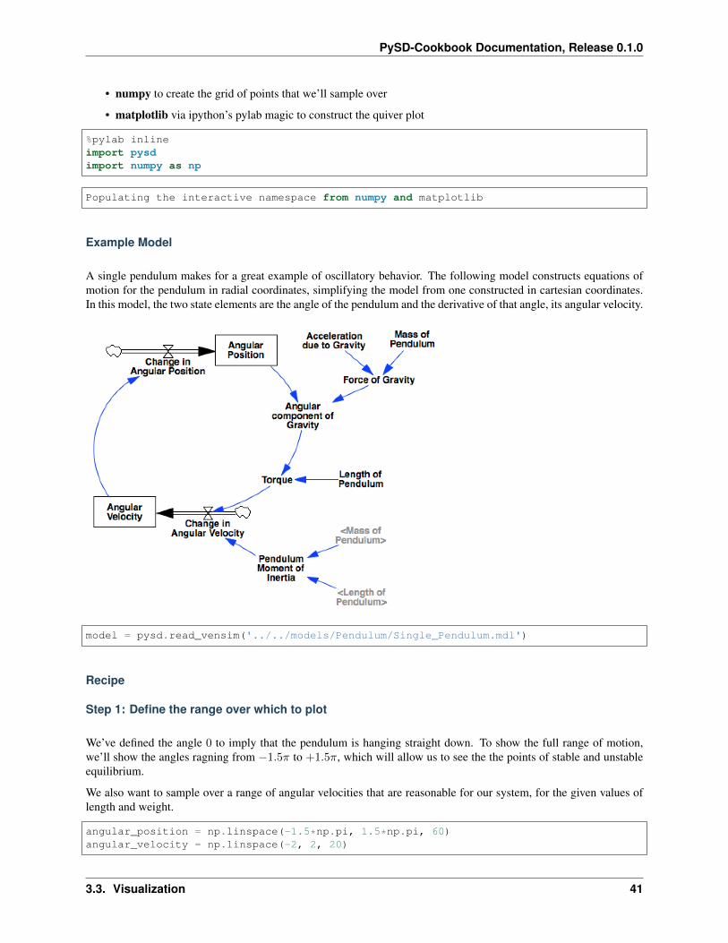
Example Model
A single pendulum makes for a great example of oscillatory behavior. The following model constructs equations ofmotion for the pendulum in radial coordinates, simplifying the model from one constructed in cartesian coordinates.In this model, the two state elements are the angle of the pendulum and the derivative of that angle, its angular velocity.
model = pysd.read_vensim('../../models/Pendulum/Single_Pendulum.mdl')
Recipe
Step 1: Define the range over which to plot
We’ve defined the angle 0 to imply that the pendulum is hanging straight down. To show the full range of motion,we’ll show the angles ragning from −1.5𝜋 to +1.5𝜋, which will allow us to see the the points of stable and unstableequilibrium.
We also want to sample over a range of angular velocities that are reasonable for our system, for the given values oflength and weight.
angular_position = np.linspace(-1.5*np.pi, 1.5*np.pi, 60)angular_velocity = np.linspace(-2, 2, 20)
3.3. Visualization 41
PySD-Cookbook Documentation, Release 0.1.0
Numpy’s meshgrid lets us construct a 2d sample space based upon our arrays
apv, avv = np.meshgrid(angular_position, angular_velocity)
Step 2: Calculate the state space derivatives at a point
We’ll define a helper function, which given a point in the state space, will tell us what the derivatives of the stateelements will be. One way to do this is to run the model over a single timestep, and extract the derivative information.In this case, the model’s stocks have only one inflow/outflow, so this is the derivative value.
As the derivative of the angular position is just the angular velocity, whatever we pass in for the av parameter shouldbe returned to us as the derivative of ap.
def derivatives(ap, av):ret = model.run(params={'angular_position':ap,
'angular_velocity':av},return_timestamps=[0,1],return_columns=['change_in_angular_position',
'change_in_angular_velocity'])
return tuple(ret.loc[0].values)
derivatives(0,1)
(1.0, -0.0)
Step 3: Calculate the state space derivatives across our sample space
We can use numpy’s vectorize to make the function accept the 2d sample space we have just created. Now we cangenerate the derivative of angular position vector dapv and that of the angular velocity vector davv. As before, thederivative of the angular posiiton should be equal to the angular velocity. We check that the vectors are equal.
vderivatives = np.vectorize(derivatives)
dapv, davv = vderivatives(apv, avv)(dapv == avv).all()
True
Step 4: Plot the phase portrait
Now we have everything we need to draw the phase portrait. We’ll use matplotlib’s quiver function, which wantsas arguments the grid of x and y coordinates, and the derivatives of these coordinates.
In the plot we see the locations of stable and unstable equilibria, and can eyeball the trajectories that the system willtake through the state space by following the arrows.
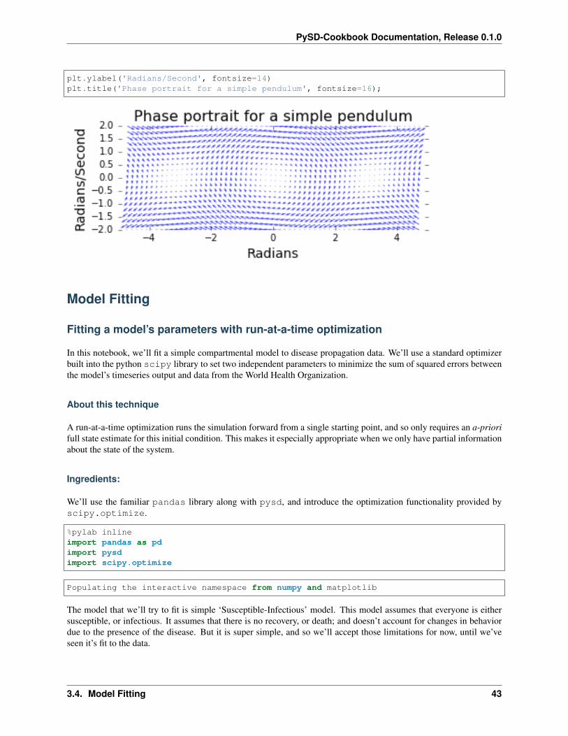
plt.figure(figsize=(18,6))plt.quiver(apv, avv, dapv, davv, color='b', alpha=.75)plt.box('off')plt.xlim(-1.6*np.pi, 1.6*np.pi)plt.xlabel('Radians', fontsize=14)
42 Chapter 3. Contents
PySD-Cookbook Documentation, Release 0.1.0
plt.ylabel('Radians/Second', fontsize=14)plt.title('Phase portrait for a simple pendulum', fontsize=16);
Model Fitting
Fitting a model’s parameters with run-at-a-time optimization
In this notebook, we’ll fit a simple compartmental model to disease propagation data. We’ll use a standard optimizerbuilt into the python scipy library to set two independent parameters to minimize the sum of squared errors betweenthe model’s timeseries output and data from the World Health Organization.
About this technique
A run-at-a-time optimization runs the simulation forward from a single starting point, and so only requires an a-priorifull state estimate for this initial condition. This makes it especially appropriate when we only have partial informationabout the state of the system.
Ingredients:
We’ll use the familiar pandas library along with pysd, and introduce the optimization functionality provided byscipy.optimize.
%pylab inlineimport pandas as pdimport pysdimport scipy.optimize
Populating the interactive namespace from numpy and matplotlib
The model that we’ll try to fit is simple ‘Susceptible-Infectious’ model. This model assumes that everyone is eithersusceptible, or infectious. It assumes that there is no recovery, or death; and doesn’t account for changes in behaviordue to the presence of the disease. But it is super simple, and so we’ll accept those limitations for now, until we’veseen it’s fit to the data.
3.4. Model Fitting 43
PySD-Cookbook Documentation, Release 0.1.0
analyses/fitting/../../../source/models/SIModel/SIModel.png
We’ll hold infectivity constant, and try to infer values for the total population and the contact frequency.
model = pysd.read_vensim('../../models/Epidemic/SI Model.mdl')
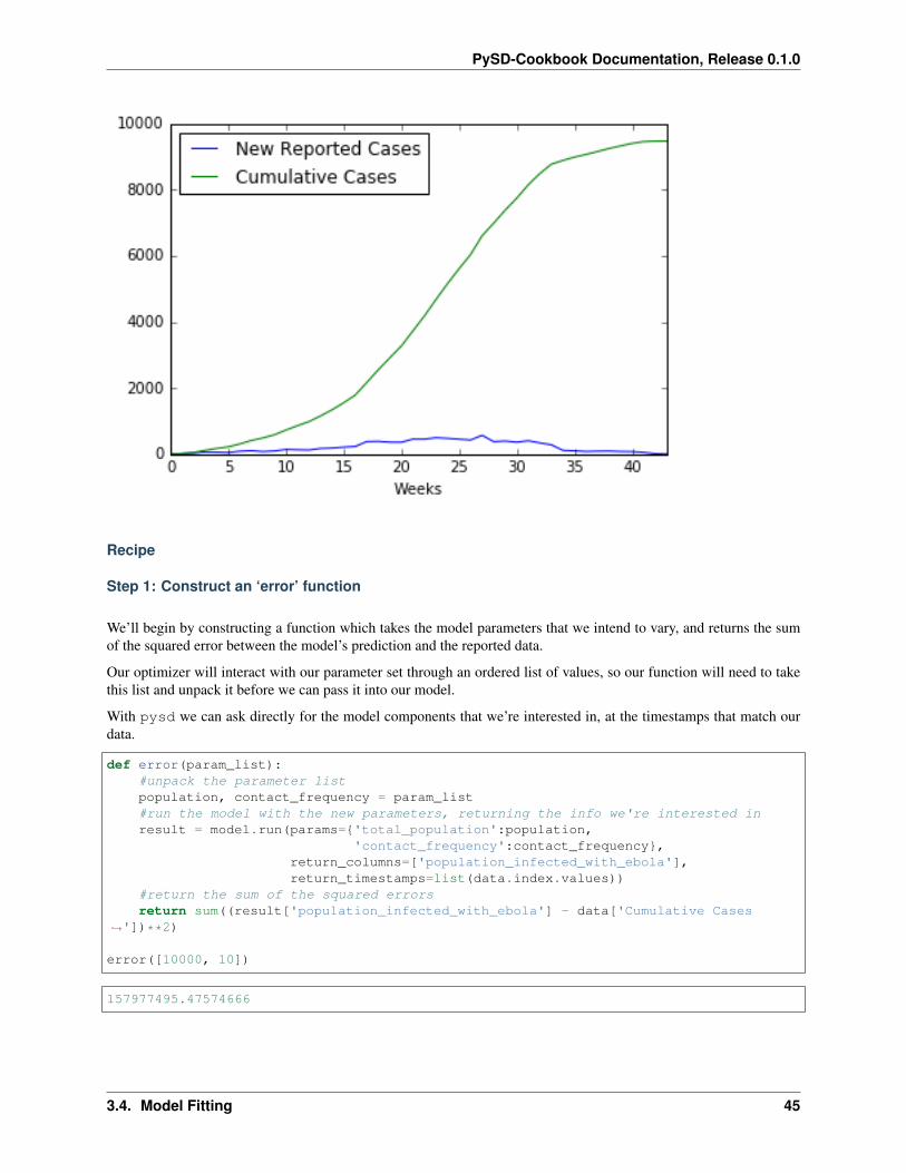
We’ll fit our model to data from the WHO patient database for Sierra Leone. We see the standard S-Shaped growth inthe cumulative infections curve. As our model has no structure for representing recovery or death, we will comparethis directly to the Population Infected with Ebola. We format this dataset in the notebook ‘Ebola Data Loader<>‘__.
data = pd.read_csv('../../data/Ebola/Ebola_in_SL_Data.csv', index_col='Weeks')data.plot();
44 Chapter 3. Contents
PySD-Cookbook Documentation, Release 0.1.0
Recipe
Step 1: Construct an ‘error’ function
We’ll begin by constructing a function which takes the model parameters that we intend to vary, and returns the sumof the squared error between the model’s prediction and the reported data.
Our optimizer will interact with our parameter set through an ordered list of values, so our function will need to takethis list and unpack it before we can pass it into our model.
With pysd we can ask directly for the model components that we’re interested in, at the timestamps that match ourdata.
def error(param_list):#unpack the parameter listpopulation, contact_frequency = param_list#run the model with the new parameters, returning the info we're interested inresult = model.run(params={'total_population':population,
'contact_frequency':contact_frequency},return_columns=['population_infected_with_ebola'],return_timestamps=list(data.index.values))
#return the sum of the squared errorsreturn sum((result['population_infected_with_ebola'] - data['Cumulative Cases
→˓'])**2)
error([10000, 10])
157977495.47574666
3.4. Model Fitting 45
PySD-Cookbook Documentation, Release 0.1.0
Step 2: Suggest a starting point and parameter bounds for the optimizer
The optimizer will want a starting point from which it will vary the parameters to minimize the error. We’ll take aguess based upon the data and our intuition.
As our model is only valid for positive parameter values, we’ll want to specify that fact to the optimizer. We knowthat there must be at least two people for an infection to take place (one person susceptible, and another contageous)and we know that the contact frequency must be a finite, positive value. We can use these, plus some reasonable upperlimits, to set the bounds.
susceptible_population_guess = 9000contact_frequency_guess = 20
susceptible_population_bounds = (2, 50000)contact_frequency_bounds = (0.001, 100)
Step 3: Minimize the error with an optimization function
We pass this function into the optimization function, along with an initial guess as to the parameters that we’re opti-mizing. There are a number of optimization algorithms, each with their own settings, that are available to us throughthis interface. In this case, we’re using the L-BFGS-B algorithm, as it gives us the ability to constrain the values theoptimizer will try.
res = scipy.optimize.minimize(error, [susceptible_population_guess,contact_frequency_guess],
method='L-BFGS-B',bounds=[susceptible_population_bounds,
contact_frequency_bounds])res
fun: 22200247.95370693hess_inv: <2x2 LbfgsInvHessProduct with dtype=float64>
jac: array([ 0. , -1666.3223505])message: 'CONVERGENCE: REL_REDUCTION_OF_F_<=_FACTR*EPSMCH'
nfev: 66nit: 10
status: 0success: True
x: array([ 8.82129606e+03, 8.20459019e+00])
Result
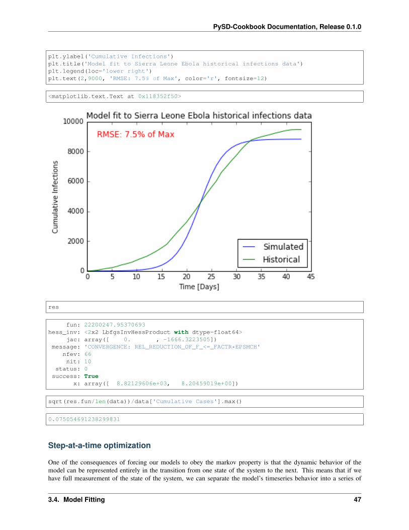
If we run the simulation with the parameters suggested by the optimizer, we see that the model follows the generalbehavior of the data, but is too simple to truly capture the correct shape of the curve.
population, contact_frequency = res.xresult = model.run(params={'total_population':population,
'contact_frequency':contact_frequency},return_columns=['population_infected_with_ebola'],return_timestamps=list(data.index.values))
plt.plot(result.index, result['population_infected_with_ebola'], label='Simulated')plt.plot(data.index, data['Cumulative Cases'], label='Historical');plt.xlabel('Time [Days]')
46 Chapter 3. Contents
PySD-Cookbook Documentation, Release 0.1.0
plt.ylabel('Cumulative Infections')plt.title('Model fit to Sierra Leone Ebola historical infections data')plt.legend(loc='lower right')plt.text(2,9000, 'RMSE: 7.5% of Max', color='r', fontsize=12)
<matplotlib.text.Text at 0x118352f50>
res
fun: 22200247.95370693hess_inv: <2x2 LbfgsInvHessProduct with dtype=float64>
jac: array([ 0. , -1666.3223505])message: 'CONVERGENCE: REL_REDUCTION_OF_F_<=_FACTR*EPSMCH'
nfev: 66nit: 10
status: 0success: True
x: array([ 8.82129606e+03, 8.20459019e+00])
sqrt(res.fun/len(data))/data['Cumulative Cases'].max()
0.075054691238299831
Step-at-a-time optimization
One of the consequences of forcing our models to obey the markov property is that the dynamic behavior of themodel can be represented entirely in the transition from one state of the system to the next. This means that if wehave full measurement of the state of the system, we can separate the model’s timeseries behavior into a series of
3.4. Model Fitting 47
PySD-Cookbook Documentation, Release 0.1.0
independent timesteps. Now we can fit the model parameters to each timestep independently, without worrying abouterrors compounding thoughout the simulation.
We’ll demonstrate this fitting of a model to data using PySD to manage our model, pandas to manage our data, andscipy to provide the optimization.
About this technique
We can use this technique when we have full state information measurements in the dataset. It is particularly helpfulfor addressing oscillatory behavior.
%pylab inlineimport pandas as pdimport pysdimport scipy.optimize
Populating the interactive namespace from numpy and matplotlib
/Users/houghton/anaconda/lib/python2.7/site-packages/pandas/computation/__init__.→˓py:19: UserWarning: The installed version of numexpr 2.4.4 is not supported in→˓pandas and will be not be used
UserWarning)
Ingredients
Model
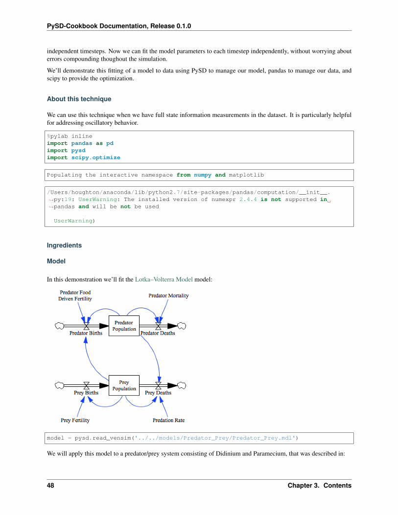
In this demonstration we’ll fit the Lotka–Volterra Model model:
model = pysd.read_vensim('../../models/Predator_Prey/Predator_Prey.mdl')
We will apply this model to a predator/prey system consisting of Didinium and Paramecium, that was described in:
48 Chapter 3. Contents
PySD-Cookbook Documentation, Release 0.1.0
Veilleux (1976) "The analysis of a predatory interaction between Didinium and→˓Paramecium", Masters thesis, University of Alberta.
There are four parameters in this model that it will be our task to set, with the goal of minimizing the sum of squarederrors between the model’s step-at-a-time prediction and the measured data.
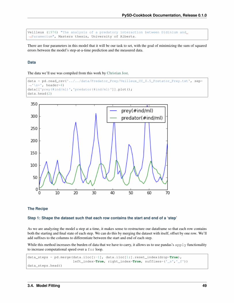
Data
The data we’ll use was compiled from this work by Christian Jost.
data = pd.read_csv('../../data/Predator_Prey/Veilleux_CC_0.5_Pretator_Prey.txt', sep=→˓'\s+', header=4)data[['prey(#ind/ml)','predator(#ind/ml)']].plot();data.head(2)
The Recipe
Step 1: Shape the dataset such that each row contains the start and end of a ‘step’
As we are analyzing the model a step at a time, it makes sense to restructure our dataframe so that each row containsboth the starting and final state of each step. We can do this by merging the dataset with itself, offset by one row. We’lladd suffixes to the columns to differentiate between the start and end of each step.
While this method increases the burden of data that we have to carry, it allows us to use pandas’s apply functionalityto increase computational speed over a for loop.
data_steps = pd.merge(data.iloc[:-1], data.iloc[1:].reset_index(drop=True),left_index=True, right_index=True, suffixes=('_s','_f'))
data_steps.head()
3.4. Model Fitting 49
PySD-Cookbook Documentation, Release 0.1.0
Step 2: Define a single-step error function
We define a function that takes a single step and calculates the sum squared error between the model’s prediction ofthe final datapoint and the actual measured value. The most complicated parts of this function are making sure that thedata columns line up properly with the model components.
Note that in this function we don’t set the parameters of the model - we can do that just once in the next function.
def one_step_error(row):result = model.run(return_timestamps=[row['time(d)_f']],
initial_condition=(row['time(d)_s'],{'predator_population':row['predator(#ind/
→˓ml)_s'],'prey_population':row['prey(#ind/ml)_s']}))
sse = ((result.loc[row['time(d)_f']]['predator_population'] - row['predator(#ind/→˓ml)_f'])**2 +
(result.loc[row['time(d)_f']]['prey_population'] - row['prey(#ind/ml)_f→˓'])**2 )
return sse
Step 3: Define an error function for the full dataset
Now we define a function that sets the parameters of the model based upon the optimizer’s suggestion, and computesthe sum squared error for all steps.
def error(parameter_list):parameter_names = ['predation_rate', 'prey_fertility', 'predator_mortality',
→˓'predator_food_driven_fertility']model.set_components(params=dict(zip(parameter_names, parameter_list)))
errors = data_steps.apply(one_step_error, axis=1)return errors.sum()
error([.005, 1, 1, .002])
545152.61053738836
Now we’re ready to use scipy’s built-in optimizer.
res = scipy.optimize.minimize(error, x0=[.005, 1, 1, .002], method='L-BFGS-B',bounds=[(0,10), (0,None), (0,10), (0,None)])
Result
We can plot the behavior of the system with our fit parameters over time:
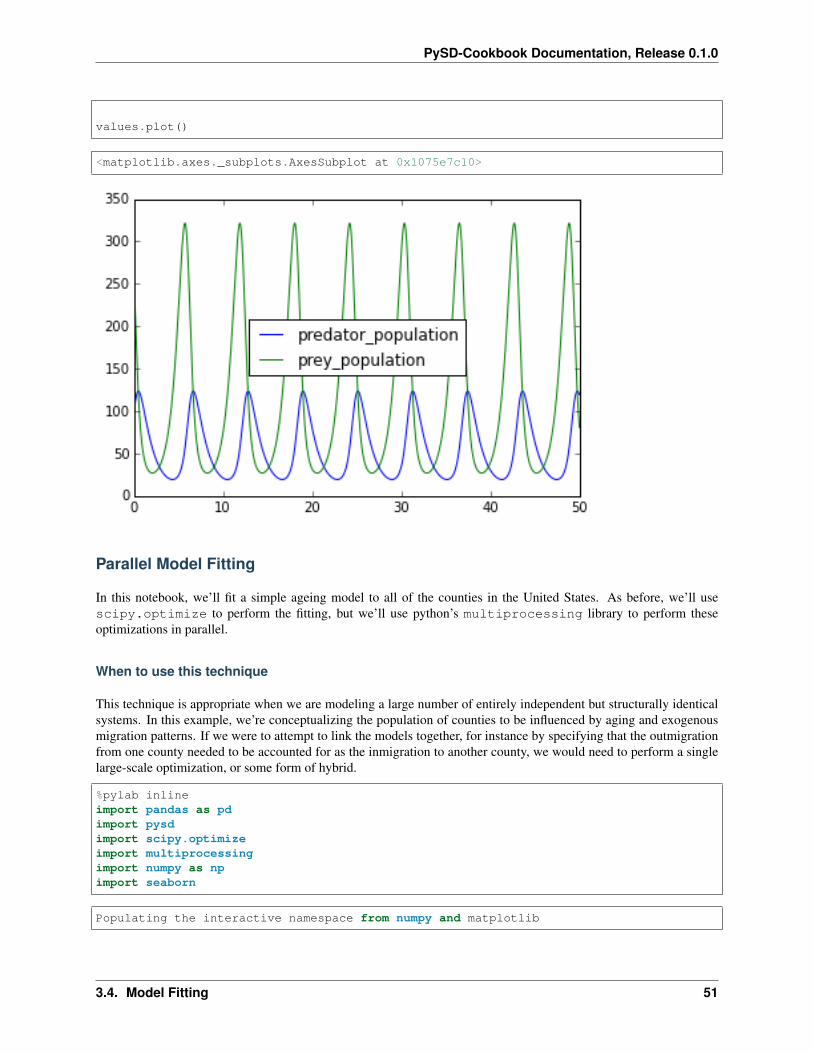
predation_rate, prey_fertility, predator_mortality, predator_food_driven_fertility =→˓res.xvalues = model.run(params={'predation_rate':predation_rate,
'prey_fertility':prey_fertility,'predator_mortality':predator_mortality,'predator_food_driven_fertility':predator_food_driven_
→˓fertility})
50 Chapter 3. Contents
PySD-Cookbook Documentation, Release 0.1.0
values.plot()
<matplotlib.axes._subplots.AxesSubplot at 0x1075e7c10>
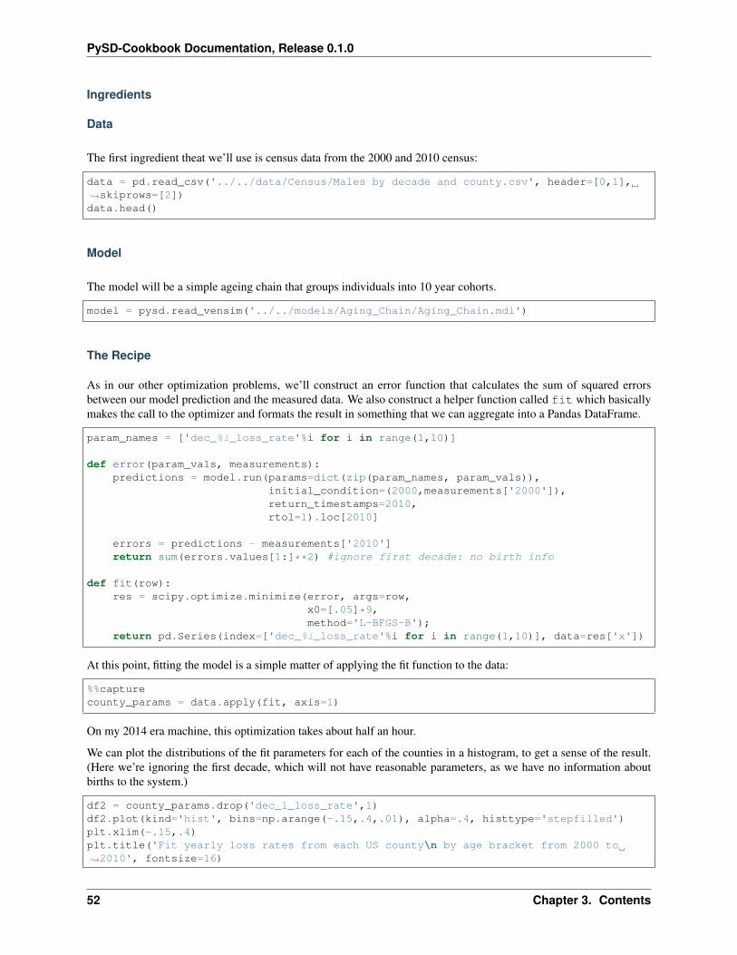
Parallel Model Fitting
In this notebook, we’ll fit a simple ageing model to all of the counties in the United States. As before, we’ll usescipy.optimize to perform the fitting, but we’ll use python’s multiprocessing library to perform theseoptimizations in parallel.
When to use this technique
This technique is appropriate when we are modeling a large number of entirely independent but structurally identicalsystems. In this example, we’re conceptualizing the population of counties to be influenced by aging and exogenousmigration patterns. If we were to attempt to link the models together, for instance by specifying that the outmigrationfrom one county needed to be accounted for as the inmigration to another county, we would need to perform a singlelarge-scale optimization, or some form of hybrid.
%pylab inlineimport pandas as pdimport pysdimport scipy.optimizeimport multiprocessingimport numpy as npimport seaborn
Populating the interactive namespace from numpy and matplotlib
3.4. Model Fitting 51
PySD-Cookbook Documentation, Release 0.1.0
Ingredients
Data
The first ingredient theat we’ll use is census data from the 2000 and 2010 census:
data = pd.read_csv('../../data/Census/Males by decade and county.csv', header=[0,1],→˓skiprows=[2])data.head()
Model
The model will be a simple ageing chain that groups individuals into 10 year cohorts.
model = pysd.read_vensim('../../models/Aging_Chain/Aging_Chain.mdl')
The Recipe
As in our other optimization problems, we’ll construct an error function that calculates the sum of squared errorsbetween our model prediction and the measured data. We also construct a helper function called fit which basicallymakes the call to the optimizer and formats the result in something that we can aggregate into a Pandas DataFrame.
param_names = ['dec_%i_loss_rate'%i for i in range(1,10)]
def error(param_vals, measurements):predictions = model.run(params=dict(zip(param_names, param_vals)),
initial_condition=(2000,measurements['2000']),return_timestamps=2010,rtol=1).loc[2010]
errors = predictions - measurements['2010']return sum(errors.values[1:]**2) #ignore first decade: no birth info
def fit(row):res = scipy.optimize.minimize(error, args=row,
x0=[.05]*9,method='L-BFGS-B');
return pd.Series(index=['dec_%i_loss_rate'%i for i in range(1,10)], data=res['x'])
At this point, fitting the model is a simple matter of applying the fit function to the data:
%%capturecounty_params = data.apply(fit, axis=1)
On my 2014 era machine, this optimization takes about half an hour.
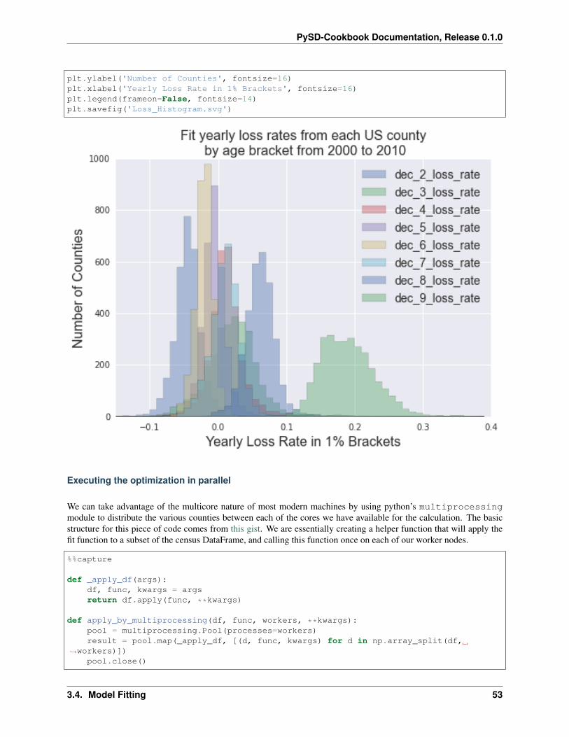
We can plot the distributions of the fit parameters for each of the counties in a histogram, to get a sense of the result.(Here we’re ignoring the first decade, which will not have reasonable parameters, as we have no information aboutbirths to the system.)
df2 = county_params.drop('dec_1_loss_rate',1)df2.plot(kind='hist', bins=np.arange(-.15,.4,.01), alpha=.4, histtype='stepfilled')plt.xlim(-.15,.4)plt.title('Fit yearly loss rates from each US county\n by age bracket from 2000 to→˓2010', fontsize=16)
52 Chapter 3. Contents
PySD-Cookbook Documentation, Release 0.1.0
plt.ylabel('Number of Counties', fontsize=16)plt.xlabel('Yearly Loss Rate in 1% Brackets', fontsize=16)plt.legend(frameon=False, fontsize=14)plt.savefig('Loss_Histogram.svg')
Executing the optimization in parallel
We can take advantage of the multicore nature of most modern machines by using python’s multiprocessingmodule to distribute the various counties between each of the cores we have available for the calculation. The basicstructure for this piece of code comes from this gist. We are essentially creating a helper function that will apply thefit function to a subset of the census DataFrame, and calling this function once on each of our worker nodes.
%%capture
def _apply_df(args):df, func, kwargs = argsreturn df.apply(func, **kwargs)
def apply_by_multiprocessing(df, func, workers, **kwargs):pool = multiprocessing.Pool(processes=workers)result = pool.map(_apply_df, [(d, func, kwargs) for d in np.array_split(df,
→˓workers)])pool.close()
3.4. Model Fitting 53
PySD-Cookbook Documentation, Release 0.1.0
return pd.concat(list(result))
county_params = apply_by_multiprocessing(data[:10], fit, axis=1, workers=4)
Fitting a model with Markov Chain Monte Carlo
Markov Chain Monte Carlo (MCMC) is a way to infer a distribution of model parameters, given that the measurementsof the output of the model are influenced by some tractable random process. In this case, performs something akin tothe opposite of what a standard Monte Carlo simultion will do. Instead of starting with distributions for the parametersof a model and using them to calculate a distribution (usually related to uncertainty) in the output of the simulation,we start with a distribution of that output and look for input distributions.
Ingredients
For this analysis we’ll introduce the python package PyMC which implements MCMC algorithms for us. Anotherproject which performs similar calculations is PyStan.
%pylab inlineimport pysdimport pymcimport pandas as pd
Populating the interactive namespace from numpy and matplotlib
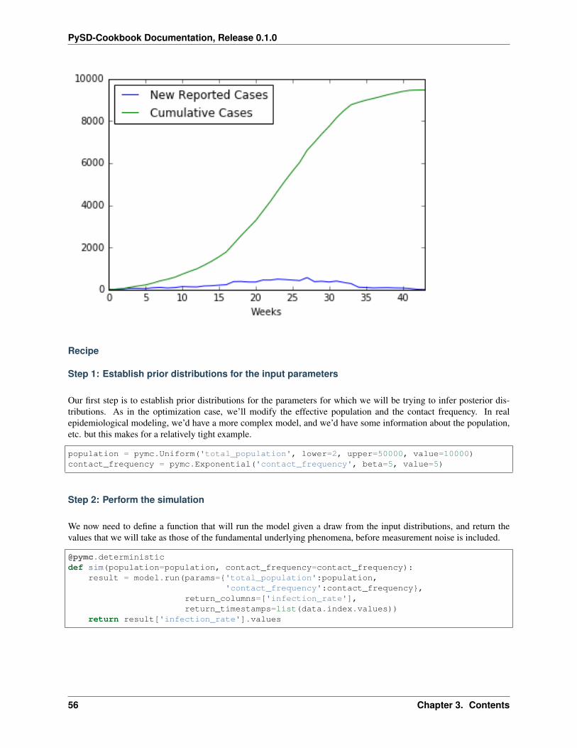
For this example, we’ll revisit the ebola case, only assuming that our data has some noise, and we’ll use MCMC toestimate distributions for the parameters for the model. For a more detailed description of this model and the datasetsee the recipe Fitting with Optimization.
We’ll assume that the model simulates an underlying process of disease propagation, but that the data is noisy - perhapsit represents admittance rates at a hospital, and so will be missing some cases, and may include some false positivesthrough misdiagnosis.
54 Chapter 3. Contents
PySD-Cookbook Documentation, Release 0.1.0
analyses/fitting/../../../source/models/SIModel/SIModel.png
model = pysd.read_vensim('../../models/SI Model/SI Model.mdl')
data = pd.read_csv('../../data/Ebola/Ebola_in_SL_Data.csv', index_col='Weeks')data.plot();
3.4. Model Fitting 55
PySD-Cookbook Documentation, Release 0.1.0
Recipe
Step 1: Establish prior distributions for the input parameters
Our first step is to establish prior distributions for the parameters for which we will be trying to infer posterior dis-tributions. As in the optimization case, we’ll modify the effective population and the contact frequency. In realepidemiological modeling, we’d have a more complex model, and we’d have some information about the population,etc. but this makes for a relatively tight example.
population = pymc.Uniform('total_population', lower=2, upper=50000, value=10000)contact_frequency = pymc.Exponential('contact_frequency', beta=5, value=5)
Step 2: Perform the simulation
We now need to define a function that will run the model given a draw from the input distributions, and return thevalues that we will take as those of the fundamental underlying phenomena, before measurement noise is included.
@pymc.deterministicdef sim(population=population, contact_frequency=contact_frequency):
result = model.run(params={'total_population':population,'contact_frequency':contact_frequency},
return_columns=['infection_rate'],return_timestamps=list(data.index.values))
return result['infection_rate'].values
56 Chapter 3. Contents
PySD-Cookbook Documentation, Release 0.1.0
Step 3: Include noise terms
There are several ways we could include noise. If we expected no false positives, we could use a Binomial distribution,such that of n possible cases that could be reported, only a fraction p would be reported, and other cases missed. Ifwe only want to model false positives, we could assume that there was an average rate of false positives, with the datafollowing a poisson distribution. The full rate would be the sum of these two processes.
For now, however, we’ll simplify the analysis by only looking at the Poisson noise component. The mean of thepoisson process will be the results of our simulation.
This is where we include our measured data into the model. PyMC will know how to calculate the log likelihood ofseeing the observed data given the assumption that the simulation result represents the underlying process, subject toPoisson noise.
admittances = pymc.Poisson('admittances', mu=sim,value=data['New Reported Cases'], observed=True)
Step 4: Perform the MCMC Sampling
Now that we have set up the problem for PyMC, we need only to run the MCMC sampler. What this will do, essentially,is take a trial set of points from our prior distribution, simulate the model, and evaluate the likelihood of the data giventhose input parameters, the simulation model, and the noise distribution. It will then use bayes law to decide whetherto keep the trial points or throw them away. It will then choose a new set of points and start over. (There is a lot morecleverness happening than this, of course. If you want to know how it works, I recommend Bayesian Methods forHackers.
First we assemble the various pieces of the data flow that we built up into a model that pymc can recognize, andinstantiate a sampler MCMC to run the algorithm for us.
Then we’ll ask the MCMC algorithm to run until it has kept 20000 points. We’ll throw out the first 1000 of these, asthey are likely to be biased towards the initial values we set up and not representative of the overall distribution.
mcmdl = pymc.Model([population, contact_frequency, sim, admittances])mcmc = pymc.MCMC(mcmdl)mcmc.sample(20000,1000)
[-----------------100%-----------------] 20000 of 20000 complete in 67.1 sec
Step 5: Look at the distribution
We can now evaluate the results by looking at the series of points we ‘kept’. These are stored as traces within thepopulation and contact frequency objects we built earlier.
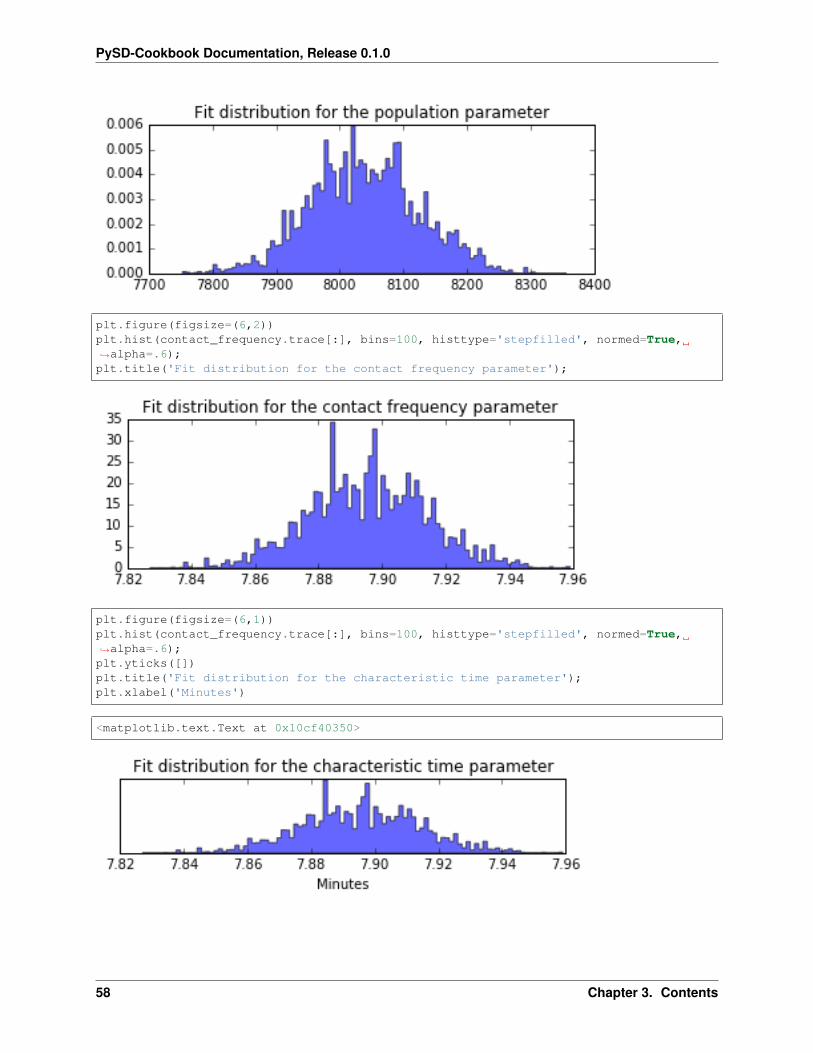
plt.figure(figsize=(6,2))plt.hist(population.trace[:], bins=100, histtype='stepfilled', normed=True, alpha=.6);plt.title('Fit distribution for the population parameter');
3.4. Model Fitting 57
PySD-Cookbook Documentation, Release 0.1.0
plt.figure(figsize=(6,2))plt.hist(contact_frequency.trace[:], bins=100, histtype='stepfilled', normed=True,→˓alpha=.6);plt.title('Fit distribution for the contact frequency parameter');
plt.figure(figsize=(6,1))plt.hist(contact_frequency.trace[:], bins=100, histtype='stepfilled', normed=True,→˓alpha=.6);plt.yticks([])plt.title('Fit distribution for the characteristic time parameter');plt.xlabel('Minutes')
<matplotlib.text.Text at 0x10cf40350>
58 Chapter 3. Contents
PySD-Cookbook Documentation, Release 0.1.0
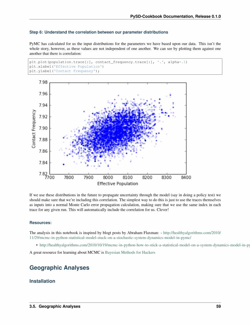
Step 6: Understand the correlation between our parameter distributions
PyMC has calculated for us the input distributions for the parameters we have based upon our data. This isn’t thewhole story, however, as these values are not independent of one another. We can see by plotting them against oneanother that there is correlation:
plt.plot(population.trace[:], contact_frequency.trace[:], '.', alpha=.1)plt.xlabel('Effective Population')plt.ylabel('Contact Frequency');
If we use these distributions in the future to propagate uncertainty through the model (say in doing a policy test) weshould make sure that we’re including this correlation. The simplest way to do this is just to use the traces themselvesas inputs into a normal Monte Carlo error propagation calculation, making sure that we use the same index in eachtrace for any given run. This will automatically include the correlation for us. Clever!
Resources:
The analysis in this notebook is inspired by blogt posts by Abraham Flaxman: - http://healthyalgorithms.com/2010/11/29/mcmc-in-python-statistical-model-stuck-on-a-stochastic-system-dynamics-model-in-pymc/
• http://healthyalgorithms.com/2010/10/19/mcmc-in-python-how-to-stick-a-statistical-model-on-a-system-dynamics-model-in-pymc/
A great resource for learning about MCMC is Bayesian Methods for Hackers
Geographic Analyses
Installation
3.5. Geographic Analyses 59
PySD-Cookbook Documentation, Release 0.1.0
conda install -c ioos geopandas=0.2.0.dev0
Using SD to understand the SD Fever
In this script, we will use georeferenced data at a national level to simulate a multiregional infectious disease model.We’ll then present the advantages to project spatial data produced by our simulation back on a map.
%matplotlib inlineimport pandas as pdimport pysd
/Users/houghton/anaconda/lib/python2.7/site-packages/pandas/computation/__init__.→˓py:19: UserWarning: The installed version of numexpr 2.4.4 is not supported in→˓pandas and will be not be used
UserWarning)
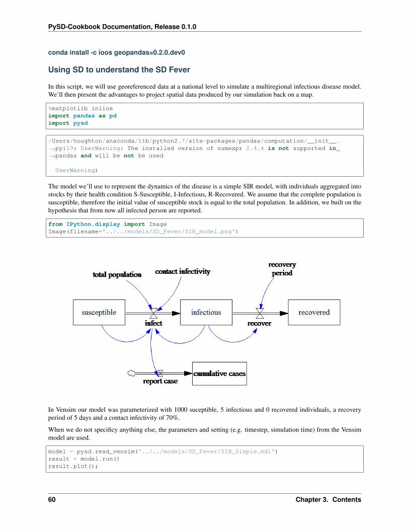
The model we’ll use to represent the dynamics of the disease is a simple SIR model, with individuals aggregated intostocks by their health condition S-Susceptible, I-Infectious, R-Recovered. We assume that the complete population issusceptible, therefore the initial value of susceptible stock is equal to the total population. In addition, we built on thehypothesis that from now all infected person are reported.
from IPython.display import ImageImage(filename='../../models/SD_Fever/SIR_model.png')
In Vensim our model was parameterized with 1000 suceptible, 5 infectious and 0 recovered individuals, a recoveryperiod of 5 days and a contact infectivity of 70%.
When we do not specificy anything else, the parameters and setting (e.g. timestep, simulation time) from the Vensimmodel are used.
model = pysd.read_vensim('../../models/SD_Fever/SIR_Simple.mdl')result = model.run()result.plot();
60 Chapter 3. Contents
PySD-Cookbook Documentation, Release 0.1.0
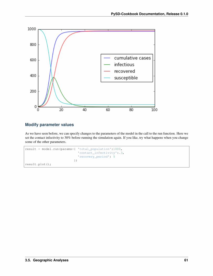
Modify parameter values
As we have seen before, we can specify changes to the parameters of the model in the call to the run function. Here weset the contact infectivity to 30% before running the simulation again. If you like, try what happens when you changesome of the other parameters.
result = model.run(params={ 'total_population':1000,'contact_infectivity':.3,'recovery_period': 5
})result.plot();
3.5. Geographic Analyses 61
PySD-Cookbook Documentation, Release 0.1.0
Change Model settings
We can also change in a very simpe manner the simulation time and timestep of the model. An easy way to do it is touse numpy linspace which returns evenly spaced numbers over a specified interval.
np.linspace(Start, Stop, Number of timestamps)
import numpy as npsim_time = 10np.linspace(0, sim_time, num=sim_time*4+1)
array([ 0. , 0.25, 0.5 , 0.75, 1. , 1.25, 1.5 , 1.75,2. , 2.25, 2.5 , 2.75, 3. , 3.25, 3.5 , 3.75,4. , 4.25, 4.5 , 4.75, 5. , 5.25, 5.5 , 5.75,6. , 6.25, 6.5 , 6.75, 7. , 7.25, 7.5 , 7.75,8. , 8.25, 8.5 , 8.75, 9. , 9.25, 9.5 , 9.75, 10. ])
We can use the return_timestamps keyword argument in PySD. This argument expects a list of timestamps, and willreturn simulation results at those timestamps.
model.run(return_timestamps=np.linspace(0, sim_time, num=sim_time*2+1))
Geographical Information
Geospatial information as area on a map linked to several properties are typically stored into shapefiles.
For this script, we will use geopandas library to manage the shapefiles, and utilize its inherent plotting functionality.
import geopandas as gp
shapefile = '../../data/SD_Fever/geo_df_EU.shp'
62 Chapter 3. Contents
PySD-Cookbook Documentation, Release 0.1.0
geo_data = gp.GeoDataFrame.from_file(shapefile)geo_data.head(5)
---------------------------------------------------------------------------
ImportError Traceback (most recent call last)
<ipython-input-7-17f6f8f07da0> in <module>()----> 1 import geopandas as gp
23 shapefile = '../../data/SD_Fever/geo_df_EU.shp'4 geo_data = gp.GeoDataFrame.from_file(shapefile)5 geo_data.head(5)
/Users/houghton/anaconda/lib/python2.7/site-packages/geopandas/__init__.pyc in→˓<module>()
2 from geopandas.geodataframe import GeoDataFrame3
----> 4 from geopandas.io.file import read_file5 from geopandas.io.sql import read_postgis6 from geopandas.tools import sjoin
/Users/houghton/anaconda/lib/python2.7/site-packages/geopandas/io/file.py in <module>→˓()
1 import os2
----> 3 import fiona4 import numpy as np5 from shapely.geometry import mapping
/Users/houghton/anaconda/lib/python2.7/site-packages/fiona/__init__.py in <module>()70 from six import string_types71
---> 72 from fiona.collection import Collection, BytesCollection, vsi_path73 from fiona._drivers import driver_count, GDALEnv, supported_drivers74 from fiona.odict import OrderedDict
/Users/houghton/anaconda/lib/python2.7/site-packages/fiona/collection.py in <module>()5 import sys6
----> 7 from fiona.ogrext import Iterator, ItemsIterator, KeysIterator8 from fiona.ogrext import Session, WritingSession9 from fiona.ogrext import (
ImportError: dlopen(/Users/houghton/anaconda/lib/python2.7/site-packages/fiona/ogrext.→˓so, 2): Library not loaded: @rpath/libtiff.5.dylibReferenced from: /Users/houghton/anaconda/lib/libgdal.1.dylibReason: Incompatible library version: libgdal.1.dylib requires version 8.0.0 or
→˓later, but libtiff.5.dylib provides version 7.0.0
Then we can project the geographic shape of the elements on a map.
3.5. Geographic Analyses 63
PySD-Cookbook Documentation, Release 0.1.0
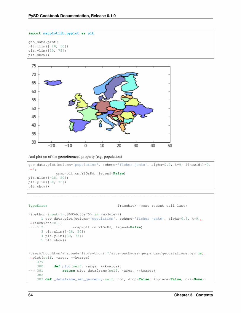
import matplotlib.pyplot as plt
geo_data.plot()plt.xlim([-28, 50])plt.ylim([30, 75])plt.show()
And plot on of the georeferenced property (e.g. population)
geo_data.plot(column='population', scheme='fisher_jenks', alpha=0.9, k=9, linewidth=0.→˓1,
cmap=plt.cm.YlOrRd, legend=False)plt.xlim([-28, 50])plt.ylim([30, 75])plt.show()
---------------------------------------------------------------------------
TypeError Traceback (most recent call last)
<ipython-input-9-c9605dc38e75> in <module>()1 geo_data.plot(column='population', scheme='fisher_jenks', alpha=0.9, k=9,
→˓linewidth=0.1,----> 2 cmap=plt.cm.YlOrRd, legend=False)
3 plt.xlim([-28, 50])4 plt.ylim([30, 75])5 plt.show()
/Users/houghton/anaconda/lib/python2.7/site-packages/geopandas/geodataframe.pyc in→˓plot(self, *args, **kwargs)
379380 def plot(self, *args, **kwargs):
--> 381 return plot_dataframe(self, *args, **kwargs)382383 def _dataframe_set_geometry(self, col, drop=False, inplace=False, crs=None):
64 Chapter 3. Contents
PySD-Cookbook Documentation, Release 0.1.0
TypeError: plot_dataframe() got an unexpected keyword argument 'linewidth'
Run the model for each country
We want to run the core SD model for each country, with country specific paramterization.
Thus, we formulate a function that based on each row parameterizes the model with the value from geodata, performsthe simulation and finally returns the number of infectious individuals over time.
def runner(row):sim_time = 200params= {'total_population':row['population'],
'contact_infectivity' : row['inf_rate']}res = model.run(params=params,
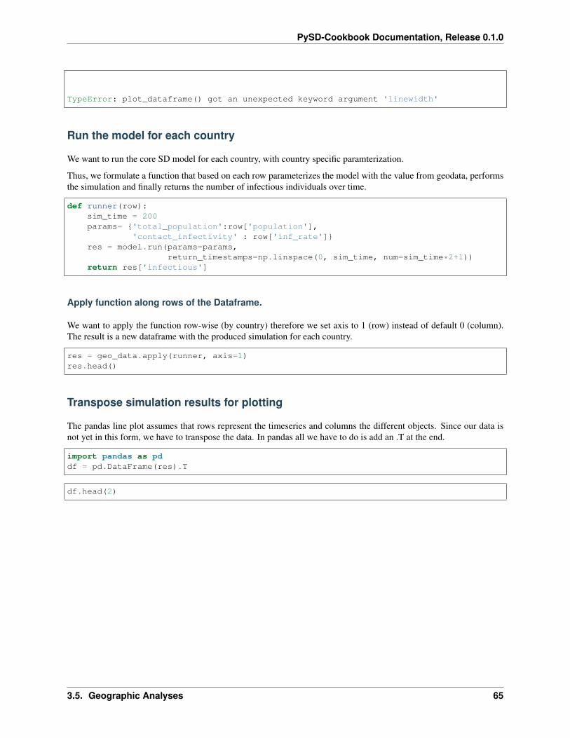
return_timestamps=np.linspace(0, sim_time, num=sim_time*2+1))return res['infectious']
Apply function along rows of the Dataframe.
We want to apply the function row-wise (by country) therefore we set axis to 1 (row) instead of default 0 (column).The result is a new dataframe with the produced simulation for each country.
res = geo_data.apply(runner, axis=1)res.head()
Transpose simulation results for plotting
The pandas line plot assumes that rows represent the timeseries and columns the different objects. Since our data isnot yet in this form, we have to transpose the data. In pandas all we have to do is add an .T at the end.
import pandas as pddf = pd.DataFrame(res).T
df.head(2)
3.5. Geographic Analyses 65
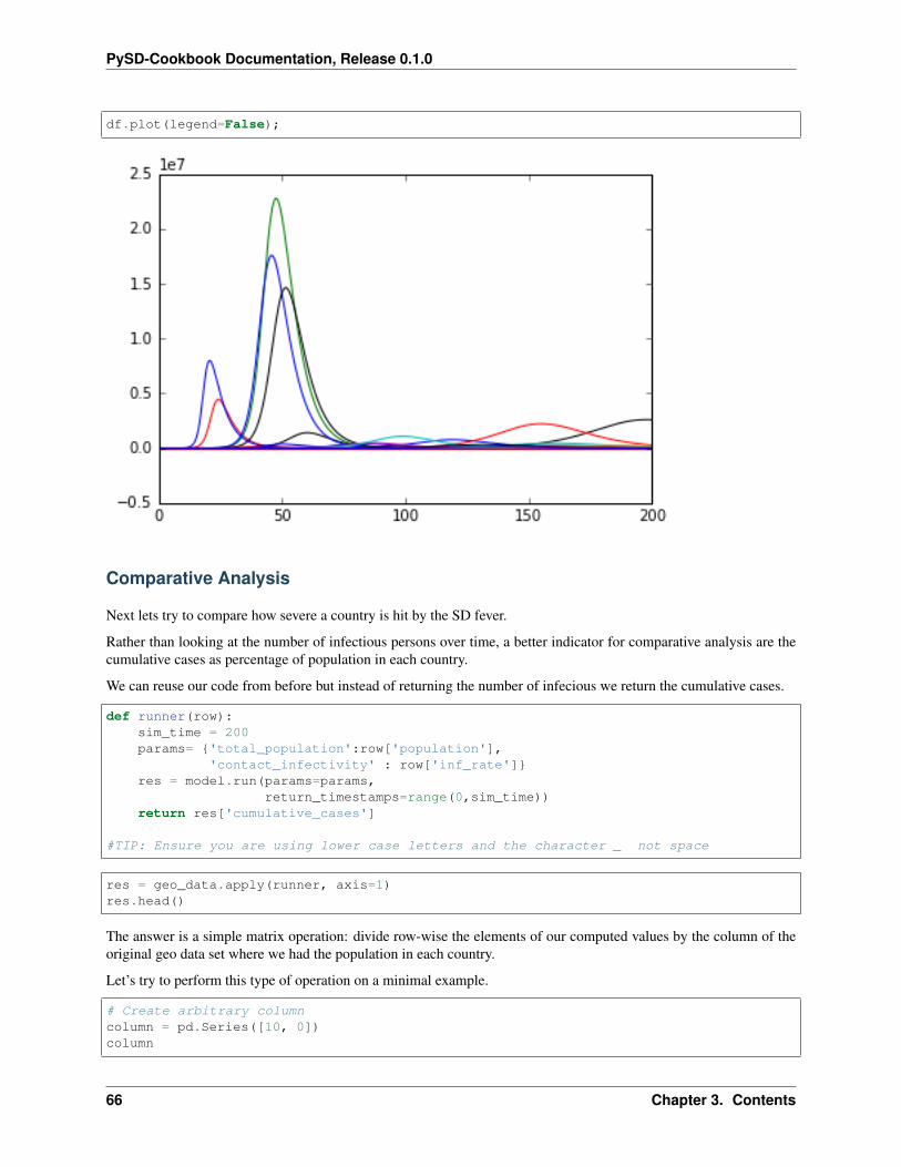
PySD-Cookbook Documentation, Release 0.1.0
df.plot(legend=False);
Comparative Analysis
Next lets try to compare how severe a country is hit by the SD fever.
Rather than looking at the number of infectious persons over time, a better indicator for comparative analysis are thecumulative cases as percentage of population in each country.
We can reuse our code from before but instead of returning the number of infecious we return the cumulative cases.
def runner(row):sim_time = 200params= {'total_population':row['population'],
'contact_infectivity' : row['inf_rate']}res = model.run(params=params,
return_timestamps=range(0,sim_time))return res['cumulative_cases']
#TIP: Ensure you are using lower case letters and the character _ not space
res = geo_data.apply(runner, axis=1)res.head()
The answer is a simple matrix operation: divide row-wise the elements of our computed values by the column of theoriginal geo data set where we had the population in each country.
Let’s try to perform this type of operation on a minimal example.
# Create arbitrary columncolumn = pd.Series([10, 0])column
66 Chapter 3. Contents
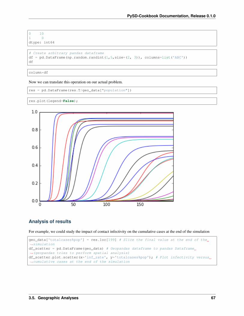
PySD-Cookbook Documentation, Release 0.1.0
0 101 0dtype: int64
# Create arbitrary pandas dataframedf = pd.DataFrame(np.random.randint(1,5,size=(2, 3)), columns=list('ABC'))df
column*df
Now we can translate this operation on our actual problem.
res = pd.DataFrame(res.T/geo_data["population"])
res.plot(legend=False);
Analysis of results
For example, we could study the impact of contact infectivity on the cumulative cases at the end of the simulation
geo_data['totalcases%pop'] = res.loc[199] # Slice the final value at the end of the→˓simulationdf_scatter = pd.DataFrame(geo_data) # Geopandas dataframe to pandas Dataframe→˓(geopandas tries to perform spatial analysis)df_scatter.plot.scatter(x='inf_rate', y='totalcases%pop'); # Plot infectivity versus→˓cumulative cases at the end of the simulation
3.5. Geographic Analyses 67
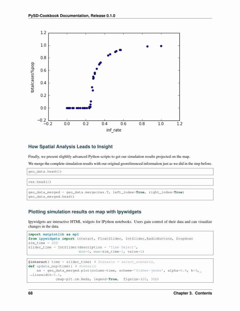
PySD-Cookbook Documentation, Release 0.1.0
How Spatial Analysis Leads to Insight
Finally, we present slighltly advanced Python scripts to get our simulation results projected on the map.
We merge the complete simulation results with our original georeferenced information just as we did in the step before.
geo_data.head(2)
res.head(2)
geo_data_merged = geo_data.merge(res.T, left_index=True, right_index=True)geo_data_merged.head()
Plotting simulation results on map with Ipywidgets
Ipywidgets are interactive HTML widgets for IPython notebooks. Users gain control of their data and can visualizechanges in the data.
import matplotlib as mplfrom ipywidgets import interact, FloatSlider, IntSlider,RadioButtons, Dropdownsim_time = 200slider_time = IntSlider(description = 'Time Select',
min=0, max=sim_time-1, value=1)
@interact( time = slider_time) # Scenario = select_scenario,def update_map(time): # Scenario
ax = geo_data_merged.plot(column=time, scheme='fisher-jenks', alpha=0.9, k=9,→˓linewidth=0.1,
cmap=plt.cm.Reds, legend=True, figsize=(20, 30))
68 Chapter 3. Contents
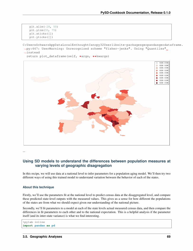
PySD-Cookbook Documentation, Release 0.1.0
plt.xlim(-28, 50)plt.ylim(30, 75)plt.xticks([])plt.yticks([])
C:UsersSchwarzAppDataLocalEnthoughtCanopy32Userlibsite-packagesgeopandasgeodataframe.→˓py:447: UserWarning: Unrecognized scheme "fisher-jenks". Using "Quantiles"→˓insteadreturn plot_dataframe(self, *args, **kwargs)
...
Using SD models to understand the differences between population measures atvarying levels of geographic disagregation
In this recipe, we will use data at a national level to infer parameters for a population aging model. We’ll then try twodifferent ways of using this trained model to understand variation between the behavior of each of the states.
About this technique
Firstly, we’ll use the parameters fit at the national level to predict census data at the disaggregated level, and comparethese predicted state-level outputs with the measured values. This gives us a sense for how different the populationsof the states are from what we should expect given our understanding of the national picture.
Secondly, we’ll fit parameters to a model at each of the state levels actual measured census data, and then compare thedifferences in fit parameters to each other and to the national expectation. This is a helpful analysis if the parameteritself (and its inter-state variance) is what we find interesting.
%pylab inlineimport pandas as pd
3.5. Geographic Analyses 69

PySD-Cookbook Documentation, Release 0.1.0
import pysdimport scipy.optimizeimport geopandas as gpd
Populating the interactive namespace from numpy and matplotlib
Ingredients
Population data by age cohort
We start with data from the decennial census years 2000 and 2010, for the male population by state and county. Wehave aggregated the data into ten-year age cohorts (with the last cohort representing everyone over 80 years old). Thedata collection task is described here. In this analysis we will only use data at the state and national levels.
data = pd.read_csv('../../data/Census/Males by decade and county.csv', header=[0,1],→˓index_col=[0,1])data.head()
A model of an aging population
The model we’ll use to represent the population is a simple aging chain, with individuals aggregated into stocks bydecade, to match the agregation we used for the above data. Each cohort is promoted with a timescale of 10 years,and there is some net inmigration, outmigration, and death subsumed into the loss flow associated with each cohort.This loss is controled by some yearly fraction that it will be our task to understand.
model = pysd.read_vensim('../../models/Aging_Chain/Aging_Chain.mdl')
Our model is initialy parameterized with 10 individuals in each stock, no births, and a uniform loss rate of 5%. We’lluse data to set the initial conditions, and infer the loss rates. Estimating births is difficult, and so for this analysis, we’llpay attention only to individuals who have been born before the year 2000.
model.run().plot();
70 Chapter 3. Contents
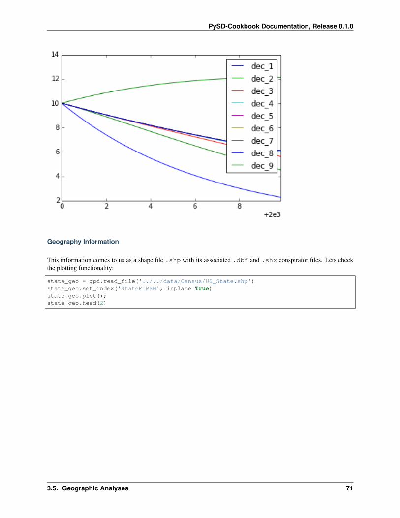
PySD-Cookbook Documentation, Release 0.1.0
Geography Information
This information comes to us as a shape file .shp with its associated .dbf and .shx conspirator files. Lets checkthe plotting functionality:
state_geo = gpd.read_file('../../data/Census/US_State.shp')state_geo.set_index('StateFIPSN', inplace=True)state_geo.plot();state_geo.head(2)
3.5. Geographic Analyses 71
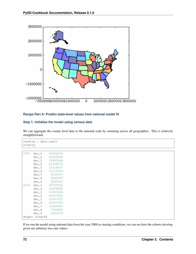
PySD-Cookbook Documentation, Release 0.1.0
Recipe Part A: Predict state-level values from national model fit
Step 1: Initialize the model using census data
We can aggregate the county level data to the national scale by summing across all geographies. This is relativelystraightforward.
country = data.sum()country
2000 dec_1 20332536dec_2 20909490dec_3 19485544dec_4 21638975dec_5 21016627dec_6 15115009dec_7 9536197dec_8 6946906dec_9 3060483
2010 dec_1 20703935dec_2 21878666dec_3 21645336dec_4 20033352dec_5 21597437dec_6 20451686dec_7 13926846dec_8 7424945dec_9 4083435
dtype: float64
If we run the model using national data from the year 2000 as starting conditions, we can see how the cohorts develop,given our arbitrary loss rate values:
72 Chapter 3. Contents
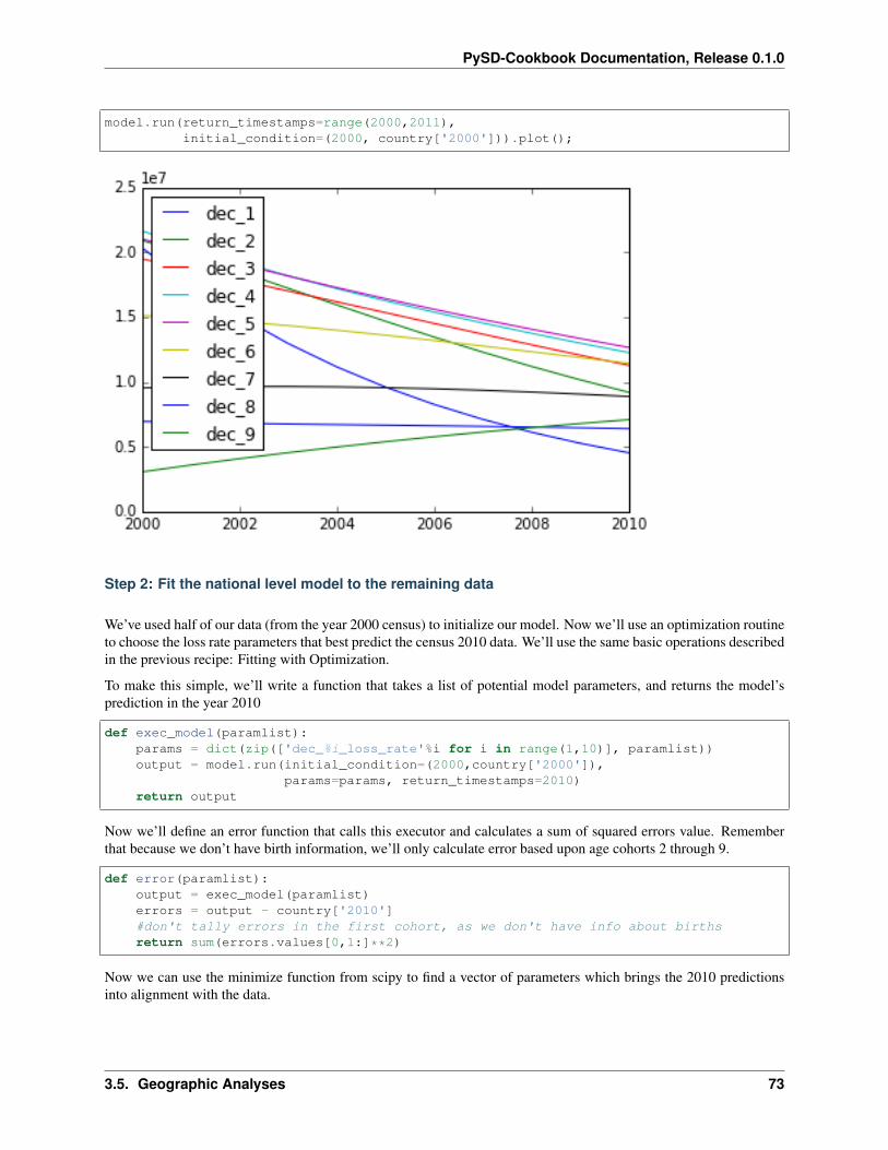
PySD-Cookbook Documentation, Release 0.1.0
model.run(return_timestamps=range(2000,2011),initial_condition=(2000, country['2000'])).plot();
Step 2: Fit the national level model to the remaining data
We’ve used half of our data (from the year 2000 census) to initialize our model. Now we’ll use an optimization routineto choose the loss rate parameters that best predict the census 2010 data. We’ll use the same basic operations describedin the previous recipe: Fitting with Optimization.
To make this simple, we’ll write a function that takes a list of potential model parameters, and returns the model’sprediction in the year 2010
def exec_model(paramlist):params = dict(zip(['dec_%i_loss_rate'%i for i in range(1,10)], paramlist))output = model.run(initial_condition=(2000,country['2000']),
params=params, return_timestamps=2010)return output
Now we’ll define an error function that calls this executor and calculates a sum of squared errors value. Rememberthat because we don’t have birth information, we’ll only calculate error based upon age cohorts 2 through 9.
def error(paramlist):output = exec_model(paramlist)errors = output - country['2010']#don't tally errors in the first cohort, as we don't have info about birthsreturn sum(errors.values[0,1:]**2)
Now we can use the minimize function from scipy to find a vector of parameters which brings the 2010 predictionsinto alignment with the data.
3.5. Geographic Analyses 73
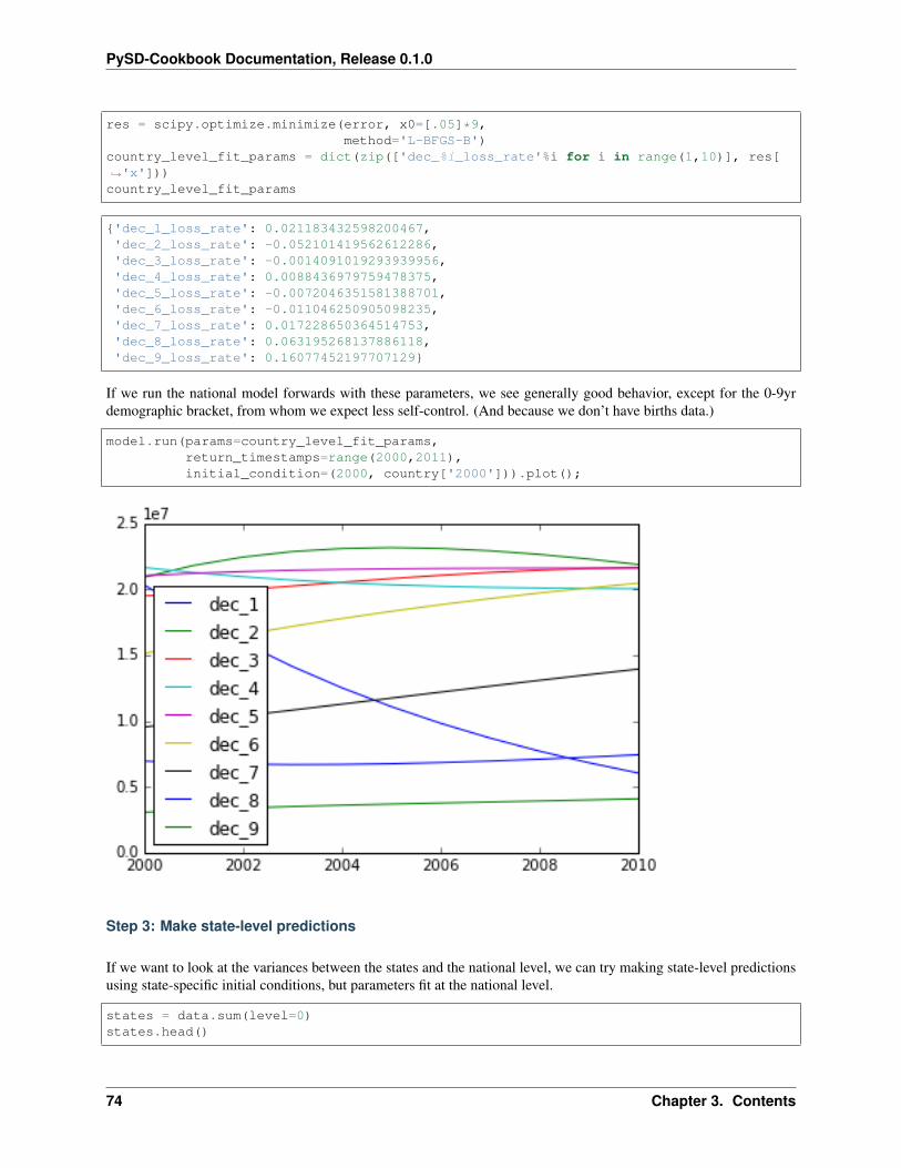
PySD-Cookbook Documentation, Release 0.1.0
res = scipy.optimize.minimize(error, x0=[.05]*9,method='L-BFGS-B')
country_level_fit_params = dict(zip(['dec_%i_loss_rate'%i for i in range(1,10)], res[→˓'x']))country_level_fit_params
{'dec_1_loss_rate': 0.021183432598200467,'dec_2_loss_rate': -0.052101419562612286,'dec_3_loss_rate': -0.0014091019293939956,'dec_4_loss_rate': 0.0088436979759478375,'dec_5_loss_rate': -0.0072046351581388701,'dec_6_loss_rate': -0.011046250905098235,'dec_7_loss_rate': 0.017228650364514753,'dec_8_loss_rate': 0.063195268137886118,'dec_9_loss_rate': 0.16077452197707129}
If we run the national model forwards with these parameters, we see generally good behavior, except for the 0-9yrdemographic bracket, from whom we expect less self-control. (And because we don’t have births data.)
model.run(params=country_level_fit_params,return_timestamps=range(2000,2011),initial_condition=(2000, country['2000'])).plot();
Step 3: Make state-level predictions
If we want to look at the variances between the states and the national level, we can try making state-level predictionsusing state-specific initial conditions, but parameters fit at the national level.
states = data.sum(level=0)states.head()
74 Chapter 3. Contents
PySD-Cookbook Documentation, Release 0.1.0
We can now generate a prediction by setting the model’s intitial conditions with state level data, and parameters fit inthe national case. I’ve created a model_runner helper function to make the code easier to read, but this could beconducted in a single line if we so chose.
def model_runner(row):result = model.run(params=country_level_fit_params,
initial_condition=(2000,row['2000']),return_timestamps=2010)
return result.loc[2010]
state_predictions = states.apply(model_runner, axis=1)state_predictions.head()
Step 4: Compare model predictions with measured data
Comparing the state level predictions with the actual data, we can see where our model most under or overpredictspopulation for each region/cohort combination.
diff = state_predictions-states['2010']diff.head()
This is a little easier to understand if we weight it by the actual measured population:
diff_percent = (state_predictions-states['2010'])/states['2010']diff_percent.head()
Step 5: Merge with geo data to plot
I’m using geopandas to manage the shapefiles, and it has its own plotting functionality. Unfortunately, it is not aparticularly well defined functionality.
geo_diff = state_geo.join(diff_percent)geo_diff.plot(column='dec_4')geo_diff.head()
3.5. Geographic Analyses 75
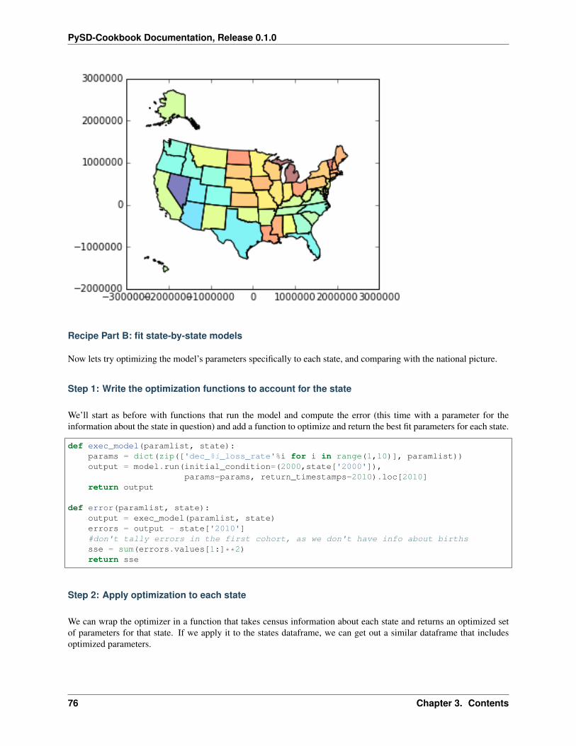
PySD-Cookbook Documentation, Release 0.1.0
Recipe Part B: fit state-by-state models
Now lets try optimizing the model’s parameters specifically to each state, and comparing with the national picture.
Step 1: Write the optimization functions to account for the state
We’ll start as before with functions that run the model and compute the error (this time with a parameter for theinformation about the state in question) and add a function to optimize and return the best fit parameters for each state.
def exec_model(paramlist, state):params = dict(zip(['dec_%i_loss_rate'%i for i in range(1,10)], paramlist))output = model.run(initial_condition=(2000,state['2000']),
params=params, return_timestamps=2010).loc[2010]return output
def error(paramlist, state):output = exec_model(paramlist, state)errors = output - state['2010']#don't tally errors in the first cohort, as we don't have info about birthssse = sum(errors.values[1:]**2)return sse
Step 2: Apply optimization to each state
We can wrap the optimizer in a function that takes census information about each state and returns an optimized setof parameters for that state. If we apply it to the states dataframe, we can get out a similar dataframe that includesoptimized parameters.
76 Chapter 3. Contents
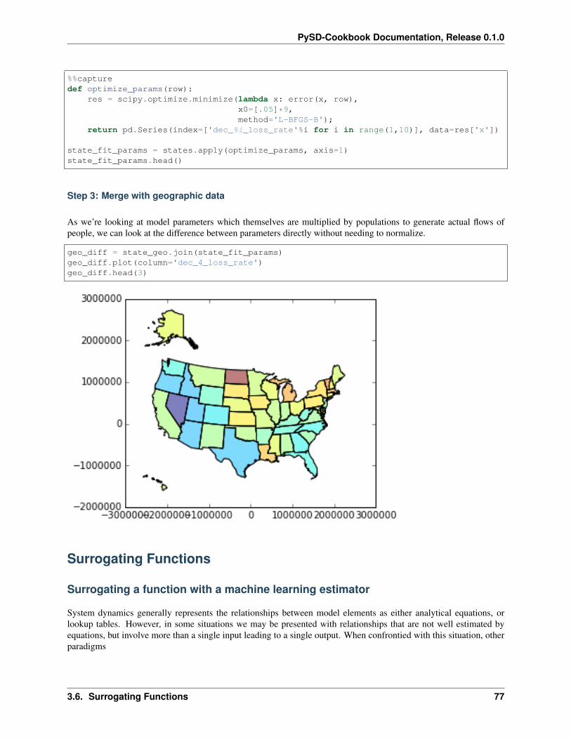
PySD-Cookbook Documentation, Release 0.1.0
%%capturedef optimize_params(row):
res = scipy.optimize.minimize(lambda x: error(x, row),x0=[.05]*9,method='L-BFGS-B');
return pd.Series(index=['dec_%i_loss_rate'%i for i in range(1,10)], data=res['x'])
state_fit_params = states.apply(optimize_params, axis=1)state_fit_params.head()
Step 3: Merge with geographic data
As we’re looking at model parameters which themselves are multiplied by populations to generate actual flows ofpeople, we can look at the difference between parameters directly without needing to normalize.
geo_diff = state_geo.join(state_fit_params)geo_diff.plot(column='dec_4_loss_rate')geo_diff.head(3)
Surrogating Functions
Surrogating a function with a machine learning estimator
System dynamics generally represents the relationships between model elements as either analytical equations, orlookup tables. However, in some situations we may be presented with relationships that are not well estimated byequations, but involve more than a single input leading to a single output. When confrontied with this situation, otherparadigms
3.6. Surrogating Functions 77
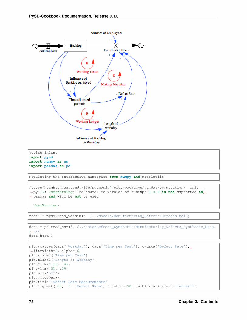
PySD-Cookbook Documentation, Release 0.1.0
%pylab inlineimport pysdimport numpy as npimport pandas as pd
Populating the interactive namespace from numpy and matplotlib
/Users/houghton/anaconda/lib/python2.7/site-packages/pandas/computation/__init__.→˓py:19: UserWarning: The installed version of numexpr 2.4.4 is not supported in→˓pandas and will be not be used
UserWarning)
model = pysd.read_vensim('../../models/Manufacturing_Defects/Defects.mdl')
data = pd.read_csv('../../data/Defects_Synthetic/Manufacturing_Defects_Synthetic_Data.→˓csv')data.head()
plt.scatter(data['Workday'], data['Time per Task'], c=data['Defect Rate'],→˓linewidth=0, alpha=.6)plt.ylabel('Time per Task')plt.xlabel('Length of Workday')plt.xlim(0.15, .45)plt.ylim(.01, .09)plt.box('off')plt.colorbar()plt.title('Defect Rate Measurements')plt.figtext(.88, .5, 'Defect Rate', rotation=90, verticalalignment='center');
78 Chapter 3. Contents
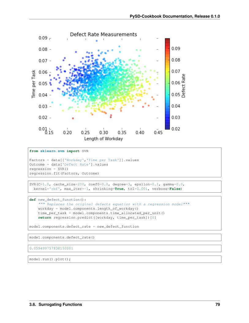
PySD-Cookbook Documentation, Release 0.1.0
from sklearn.svm import SVR
Factors = data[['Workday','Time per Task']].valuesOutcome = data['Defect Rate'].valuesregression = SVR()regression.fit(Factors, Outcome)
SVR(C=1.0, cache_size=200, coef0=0.0, degree=3, epsilon=0.1, gamma=0.0,kernel='rbf', max_iter=-1, shrinking=True, tol=0.001, verbose=False)
def new_defect_function():""" Replaces the original defects equation with a regression model"""workday = model.components.length_of_workday()time_per_task = model.components.time_allocated_per_unit()return regression.predict([workday, time_per_task])[0]
model.components.defect_rate = new_defect_function
model.components.defect_rate()
0.059499757838150001
model.run().plot();
3.6. Surrogating Functions 79
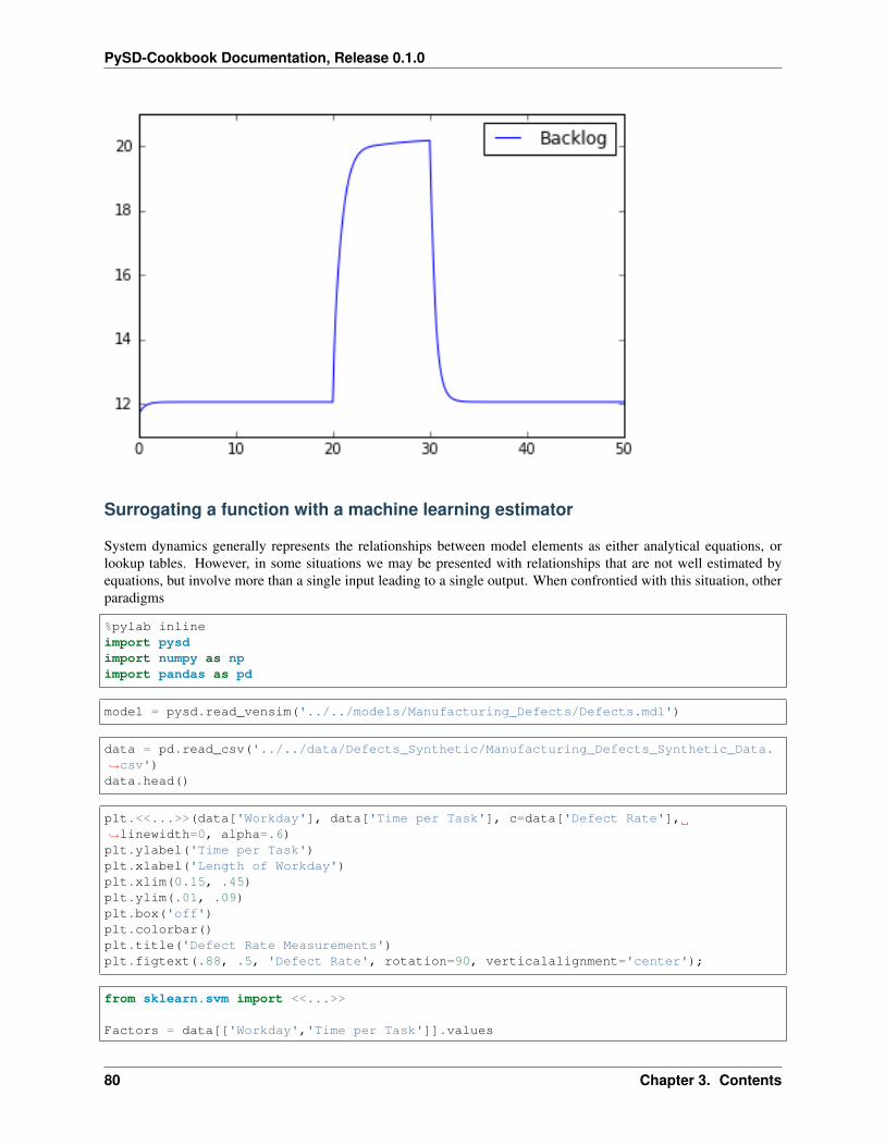
PySD-Cookbook Documentation, Release 0.1.0
Surrogating a function with a machine learning estimator
System dynamics generally represents the relationships between model elements as either analytical equations, orlookup tables. However, in some situations we may be presented with relationships that are not well estimated byequations, but involve more than a single input leading to a single output. When confrontied with this situation, otherparadigms
%pylab inlineimport pysdimport numpy as npimport pandas as pd
model = pysd.read_vensim('../../models/Manufacturing_Defects/Defects.mdl')
data = pd.read_csv('../../data/Defects_Synthetic/Manufacturing_Defects_Synthetic_Data.→˓csv')data.head()
plt.<<...>>(data['Workday'], data['Time per Task'], c=data['Defect Rate'],→˓linewidth=0, alpha=.6)plt.ylabel('Time per Task')plt.xlabel('Length of Workday')plt.xlim(0.15, .45)plt.ylim(.01, .09)plt.box('off')plt.colorbar()plt.title('Defect Rate Measurements')plt.figtext(.88, .5, 'Defect Rate', rotation=90, verticalalignment='center');
from sklearn.svm import <<...>>
Factors = data[['Workday','Time per Task']].values
80 Chapter 3. Contents
PySD-Cookbook Documentation, Release 0.1.0
Outcome = data['Defect Rate'].valuesregression = SVR()regression.<<..>>(Factors, Outcome)
def new_defect_function():""" Replaces the original defects equation with a regression model"""workday = model.<<...>>.length_of_workday()time_per_task = model.components.time_allocated_per_unit<<...>>return regression.predict([<<...>>])[0]
model.components.defect_rate = <<...>>
print model.components.defect_rate()
model.run().plot();
Realtime Data Incorporation
Nth Order Delay Demo
This is a fun demonstration designed to build intuition around the idea that balancing feedback loops with delays leadto oscillation. It uses a vensim model as the ‘system’ but provides a way for a user to interact with the simulation inrealtime - essentially acting as the controller - a balancing feedback loop around the model output.
About this Technique
This is a way to interact with the models in realtime using your keyboard.
Ingredients
The Game
The student is asked to use the ‘up’ and ‘down’ arrow keys to bring a blue line (the system output) to the value of thedashed red line (the target). However, the inputs from the keyboard go through a delay process (here using either the‘first order delay’ model, or the ‘third order delay’ model).
When we run this cell, the student will have 60 seconds to bring the blue line to the level of the red line.
%pylabimport pysdfrom matplotlib import animationimport numpy as np
Using matplotlib backend: MacOSXPopulating the interactive namespace from numpy and matplotlib
#import the model (need to import each time to reinitialize)#choose one of the following lines:#model = pysd.read_vensim('../../models/Basic_Structures/First_Order_Delay.mdl')model = pysd.read_vensim('../../models/Basic_Structures/Third_Order_Delay.mdl')
3.7. Realtime Data Incorporation 81
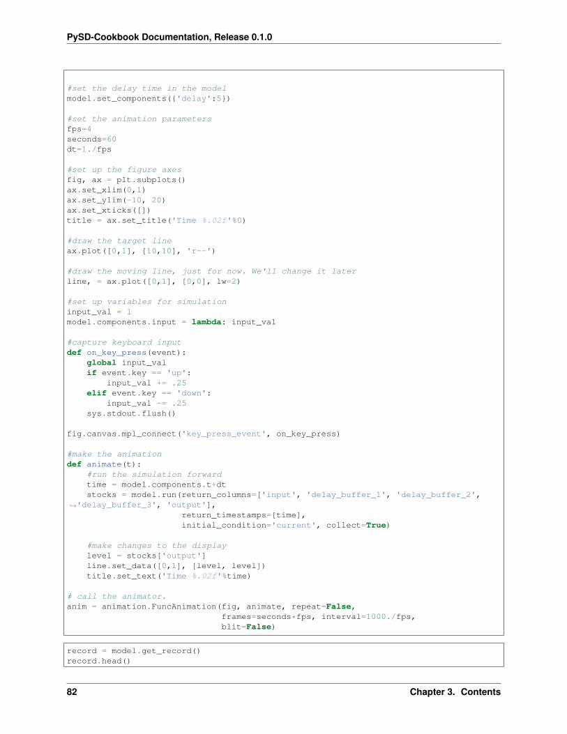
PySD-Cookbook Documentation, Release 0.1.0
#set the delay time in the modelmodel.set_components({'delay':5})
#set the animation parametersfps=4seconds=60dt=1./fps
#set up the figure axesfig, ax = plt.subplots()ax.set_xlim(0,1)ax.set_ylim(-10, 20)ax.set_xticks([])title = ax.set_title('Time %.02f'%0)
#draw the target lineax.plot([0,1], [10,10], 'r--')
#draw the moving line, just for now. We'll change it laterline, = ax.plot([0,1], [0,0], lw=2)
#set up variables for simulationinput_val = 1model.components.input = lambda: input_val
#capture keyboard inputdef on_key_press(event):
global input_valif event.key == 'up':
input_val += .25elif event.key == 'down':
input_val -= .25sys.stdout.flush()
fig.canvas.mpl_connect('key_press_event', on_key_press)
#make the animationdef animate(t):
#run the simulation forwardtime = model.components.t+dtstocks = model.run(return_columns=['input', 'delay_buffer_1', 'delay_buffer_2',
→˓'delay_buffer_3', 'output'],return_timestamps=[time],initial_condition='current', collect=True)
#make changes to the displaylevel = stocks['output']line.set_data([0,1], [level, level])title.set_text('Time %.02f'%time)
# call the animator.anim = animation.FuncAnimation(fig, animate, repeat=False,
frames=seconds*fps, interval=1000./fps,blit=False)
record = model.get_record()record.head()
82 Chapter 3. Contents
PySD-Cookbook Documentation, Release 0.1.0
record.plot();
<matplotlib.axes._subplots.AxesSubplot at 0x10f08a250>
Display student input vs model output
To show how we did, we can plot the input and output over time. Here we start to see the oscillatory behavior (forhigher order and longer delays)
plt.plot(x,input_collector, label='Your Input')plt.plot(x,y, label='Model Response')plt.legend(loc='lower right')plt.xlabel('Time [Seconds]')plt.ylabel('Value');
<matplotlib.text.Text at 0x108ab4bd0>
Display the value of each of the buffer stocks over time
If we plot the stock levels over time, we can see (especially for the third order case) how the delay works to smoothout the input values.
import pandas as pddelay_stock_values = pd.DataFrame(stocks_collector)delay_stock_values.plot()plt.xlabel('Time [Seconds]')plt.ylabel('Stock Level');
<matplotlib.text.Text at 0x108c7c590>
Feeding models with realtime streaming data
In this example, we’ll construct a very simple model of the number of posts relating to a given topic on twitter timelinesaround the world. We’ll feed the model with live streaming data from the twitter API and run the model in real time.
Ingredients
Libraries
In addition to our standard data analytics stack, we’ll take advantage of the tweepy library for interacting with thetwitter API, the standard python library for dealing with JSON objects, and the standard python threading library, togive us access to both the stream and the plots in real time.
%pylabimport tweepyimport jsonimport pysd
3.7. Realtime Data Incorporation 83
PySD-Cookbook Documentation, Release 0.1.0
import threadingfrom matplotlib import animation
Using matplotlib backend: MacOSXPopulating the interactive namespace from numpy and matplotlib
Twitter Credentials
If you want to execute this recipe, you’ll need to sign up for a twitter developer account and create a file containingyour credentials.
Name this file _twitter_credentials.py and save it in the working directory. It should contain somethingsimilar to:
consumer_key = 'sdjfhkdgjhsk8u09wejne4vdj8j34'consumer_secret = 'nvjsdv8wp43nneri'access_token = 'vndisoerihosfdbuttonmashingjkfdlasnvei'access_token_secret = 'navdjewrjodfjkmorebuttonmashingnjkasdoinv'
We can load these into our environment using the import * syntax.
from _twitter_credentials import *
Model
Our model is a simple delay process. The inflow of the process is the rate at which twitter users post messagescontaining our keywords, and the level decays over time as posts fall out of the top of users timelines.
We’ll explicitly set the timescale in this demo, to show the behavior of the system in a short timeperiod.
model = pysd.read_vensim('../../models/Twitter/Twitter.mdl')model.set_components({'displacement_timescale':30})
The Recipe
Listening to twitter
The first thing we’ll do is to create a variable that will track the total number of posts recieved in the last modelinteration timeperiod. This counter will be reset after every model timestep.
counter = 0
Next, we’ll construct a function that will be run whenever a tweet is recieved from the API. This function will increasethe counter value, and format the tweet to print to the screen.
class TweetListener(tweepy.StreamListener):def on_data(self, data):
global countercounter += 1
# Twitter returns data in JSON format - we need to decode it firstdecoded = json.loads(data)
84 Chapter 3. Contents
PySD-Cookbook Documentation, Release 0.1.0
# Also, we convert UTF-8 to ASCII ignoring all bad characters sent by usersprint '@%s: %s\n' % (decoded['user']['screen_name'], decoded['text'].encode(
→˓'ascii', 'ignore'))return True
def on_error(self, status):print status
The tweepy library manages formatting our credentials for the API request:
auth = tweepy.OAuthHandler(consumer_key, consumer_secret)auth.set_access_token(access_token, access_token_secret)
Finally we create the object that will parse the twitter stream, and start it within its own thread.
stream = tweepy.Stream(auth, TweetListener())
t = threading.Thread(target=stream.filter, kwargs={'track':['ISDC', 'PySD', 'ISDC15',→˓'Trump']})t.daemon = Truet.start()
Animation
First we create a function that will be called at every step in the integration:
#make the animationdef animate(t):
global counter#run the simulation forwardtime = model.components.t+dtmodel.run({'tweeting':counter},
return_timestamps=time,return_columns=['tweeting', 'posts_on_timeline'],initial_condition='current',collect=True)
out = model.get_record()ax.plot(out['tweeting'], 'r', label='Tweeting')ax.plot(out['posts_on_timeline'], 'b', label='Posts on Timeline')counter = 0
@alisonjpotter: RT @queenfeminist: Retweet for Bernie Sanders fav for Hillary Clinton
Ignore and Donald Trump wins
@MrTommyCampbell: RT @swhammerhead: #WhenTrumpIsElected the letter H will be removed→˓from the American lexicon as Trump doesn't pronounce it anyways. It wil
@JBRichard50: RT @BradThor: "It's impossible for Perry to have stayed gov of TX for→˓so long if he really is the person we saw in those debates." http://t
@AdeboyeOriade: RT @politicususa: President Obama Rips Donald Trump, Mike Huckabee,→˓and The Entire Republican Party http://t.co/krMZwVV1u0 via @politicusus
@1baldeagle77: The one thing that makes me take Donald Trump seriously as a candidate→˓ Rush Limbaugh http://t.co/VxDAyO8xw7 via @voxdotcom
3.7. Realtime Data Incorporation 85
PySD-Cookbook Documentation, Release 0.1.0
Lastly we set the parameters for the animation, set up the figure, reset the counter (which has been accumulating postssince we ran the first part of the code) and start the animation.
#set the animation parametersfps=1seconds=60*30dt=1./fps
#set up the plotfig, ax = plt.subplots()ax.set_xlim(0,seconds)title = ax.set_title('Expected Twitter Messages on First Page of Feed')ax.set_xlabel('Seconds')ax.set_ylabel('Posts, Posts/second')
#reset the counter to start fresh.counter=0
# call the animator.animation.FuncAnimation(fig, animate, repeat=False,
frames=seconds*fps, interval=1000./fps,blit=False)
@shehelby: RT @ProBirdRights: How can they say me a bird can not be run for→˓Presindent when Donal Trump a giant talking corn can??? #birb2016
@LacrosseUpdate: Hope Hicks flies quietly in the eye of the Trump storm http://t.co/→˓SSUZKcyyiG http://t.co/3MlnhhsEwc
@thedancingqueer: RT @queenfeminist: Retweet for Bernie Sanders fav for Hillary→˓Clinton
Ignore and Donald Trump wins
@BuzzFeedAndrew: "Never a Bush fan," Donald Trump campaigned for H.W. in 1988 held a→˓fundraiser for Jeb in 2002. http://t.co/7S2u6eSyrN
@david_alman: Fucking leftist media spends so much time covering Donald Trump's→˓statements from 20 years ago that it neglects like...anything relevant.
@kcasa7131: RT @pdacosta: #WhenTrumpIsElected, he might appoint himself as Chairman→˓of the Federal Reserve, and begin to issue Trump dollars. http://t.
@presidentrumped: President Trump: Mr Trump is a Gemini this means he is TOTALLY→˓unpredictable! http://t.co/tP5lraAyUH
@MicheleUpdate: Nicolle Wallace: Trump Is 'Doing One Thing Really, Really Well' http:/→˓/t.co/kLfGNkCqyh
@jjyorktown: RT @ConanOBrien: Im on vacation. Please keep Trump popular while Im gone,→˓ I need him in the debates.
@MisaelDiazMLM: .@amazonmex @jcgs68 @amazon Amazon: Dejen de vender los libros de→˓Donald Trump! - Firm la Peti... https://t.co/UMSTq5AxY2 va @Change_M
@StrongerForce: RT @BradThor: "It's impossible for Perry to have stayed gov of TX for→˓so long if he really is the person we saw in those debates." http://t
86 Chapter 3. Contents
PySD-Cookbook Documentation, Release 0.1.0
@cheyannebiancab: RT @bigmacher: #WhenTrumpIsElected everyone will get a Trump action→˓figure that will buy all your play houses & then goes bankrupt. http://
@BigEers: RT @Mediaite: Chris Christie Will No Longer Comment Publicly on Donald→˓Trump http://t.co/UrfQEfGklZ (AUDIO) http://t.co/5fEw69cvM7
@_miramira93: RT @SockHimBopHer: Bill Cosby's legacy is dead.. Donald Trump can→˓possibly be the president.. The Klan is traveling like an AAU team.. And
@paigekathstev: RT @ConanOBrien: Im on vacation. Please keep Trump popular while Im→˓gone, I need him in the debates.
@BMLewis2: RT @GStuedler: I cant see it happening, but in the slim chance it doesa→˓Donald Trump nomination would mean they have completely given up.
@DebndanfarrDeb: Donald Trump Surges to Lead in NH GOP Presidential Poll, Erases→˓Another's Iowa Lead - The Political Insider http://t.co/3exB1TrjPJ via
<matplotlib.animation.FuncAnimation at 0x114fc0c90>
Model Development Workflow
Unit Testing
In this notebook we’ll demonstrate some basic unit testing for models.
We build on the standard python unittest libarary, which is documented here. Other testing suites are available, withtheir own advantages, but this is the most basic, so we’ll use it for our demonstration.
Unit testing us usually done not in the ipython notebook, but in a standalone python file. Tests for this demo are foundin the accompanying file testsite.py:
import pysdimport unittest
class TestTeacupModel(unittest.TestCase):""" Test Import functionality """@classmethoddef set_up_class(cls):
cls.model = pysd.read_vensim('../../models/Teacup/Teacup.mdl')
def test_initialization(self):self.assertEqual(self.model.components.state['teacup_temperature'],180.0)
def test_heatflow_calc(self):self.assertEqual(self.model.components.heat_loss_to_room(), 11.0)
def test_output(self):self.assertAlmostEqual(self.model.run()['teacup_temperature'].iloc[-1],
75, delta=1)
if __name__ == '__main__':unittest.main()
3.8. Model Development Workflow 87
PySD-Cookbook Documentation, Release 0.1.0
%run testsuite.py
...----------------------------------------------------------------------Ran 3 tests in 0.053s
OK
Data Used in this Cookbook
All of the data used in these notebooks was either gathered from public sources, or is created synthetically for thepurpose of this cookbook. The notebooks listed here show how each set was collected or generated.
Baby Name Data
This notebook formats data from the social security administration baby names database into a format that is easy forthe cookbook to deal with. It expects the zip file to be unpacked into a subfolder called ‘names’.
import pandas as pdimport glob
filenames = glob.glob('names/yob*')
females = pd.DataFrame()males = pd.DataFrame()
for filename in filenames:year = filename[9:13]data = pd.read_csv(filename, header=None, names=['Name','Gender',year], index_col=
→˓'Name')females = females.join(data[data['Gender']=='F'].drop('Gender', axis=1), how=
→˓'outer')males = males.join(data[data['Gender']=='M'].drop('Gender', axis=1), how='outer')
females.to_csv('female_names_timeseries.csv')males.to_csv('male_names_timeseries.csv')
Collecting US decennial census data
In this notebook, we’ll collect demographic data from the US decennial census, by county.
The census website has an API, which is good, because everything else about the census website is close to unusable.The api is described here: http://www.census.gov/data/developers/data-sets/decennial-census-data.html
As a quick demonstration, we can use the API to get population data for every county in the US:
import pandas as pd
df = pd.read_json('http://api.census.gov/data/2010/sf1?get=P0120001&for=county:*')df.columns = df.iloc[0]
88 Chapter 3. Contents
PySD-Cookbook Documentation, Release 0.1.0
df.drop(df.index[0], inplace=True)df.head()
The census code descriptions can also be accessed via the API. A listing of the field names is available here: http://api.census.gov/data/2010/sf1/variables.html
pd.read_json('http://api.census.gov/data/2010/sf1/variables/P0120001.json', typ='ser')
concept P12. Sex By Age [49]label Total populationname P0120001dtype: object
Collect data on male population by age, county
For now I’m only going to look at males. This is probably a bad idea in general.
Start with the 2010 census
The male population is broken down into some somewhat arbitrary cohorts, each with its own name. We want all ofthe fields between P0120003 and P0120025.
We’ll do some data munging to get it in numeric format, and to take care of the labels and indicies.
fields = ['P01200%02i'%i for i in range(3,26)]url = 'http://api.census.gov/data/2010/sf1?get=%s&for=county:*'%','.join(fields)print urlpops2010 = pd.read_json(url)pops2010.columns = pops2010.iloc[0]pops2010.drop(pops2010.index[0], inplace=True)pops2010 = pops2010.applymap(float)pops2010.set_index(['state', 'county'], inplace=True)pops2010.head()
http://api.census.gov/data/2010/sf1?get=P0120003,P0120004,P0120005,P0120006,P0120007,→˓P0120008,P0120009,P0120010,P0120011,P0120012,P0120013,P0120014,P0120015,P0120016,→˓P0120017,P0120018,P0120019,P0120020,P0120021,P0120022,P0120023,P0120024,P0120025&→˓for=county:*
Get data from 2000
The 2000 census (logically) has different codes for its data, and (even more logically) breaks the cohorts down differ-ently. In this case, we can get data for each age year with codes PCT012003 through PCT012104. The api limitsus to only 50 columns at a time, so we’ll do it in chunks and stitch them together.
fields = ['PCT012%03i'%i for i in range(3,105)]
dflist = []chunkSize = 40for i in range(0, len(fields), chunkSize):
chunk = fields[i:i+chunkSize]url = 'http://api.census.gov/data/2000/sf1?get=%s&for=county:*'%','.join(chunk)
3.9. Data Used in this Cookbook 89
PySD-Cookbook Documentation, Release 0.1.0
print urldf_chunk = pd.read_json(url)df_chunk.columns = df_chunk.iloc[0]df_chunk.drop(df_chunk.index[0], inplace=True)df_chunk = df_chunk.applymap(float)df_chunk.set_index(['state', 'county'], inplace=True)dflist.append(df_chunk)
pops2000 = pd.concat(dflist,axis=1)pops2000 = pops2000.applymap(float)pops2000.head()
http://api.census.gov/data/2000/sf1?get=PCT012003,PCT012004,PCT012005,PCT012006,→˓PCT012007,PCT012008,PCT012009,PCT012010,PCT012011,PCT012012,PCT012013,PCT012014,→˓PCT012015,PCT012016,PCT012017,PCT012018,PCT012019,PCT012020,PCT012021,PCT012022,→˓PCT012023,PCT012024,PCT012025,PCT012026,PCT012027,PCT012028,PCT012029,PCT012030,→˓PCT012031,PCT012032,PCT012033,PCT012034,PCT012035,PCT012036,PCT012037,PCT012038,→˓PCT012039,PCT012040,PCT012041,PCT012042&for=county:*http://api.census.gov/data/2000/sf1?get=PCT012043,PCT012044,PCT012045,PCT012046,→˓PCT012047,PCT012048,PCT012049,PCT012050,PCT012051,PCT012052,PCT012053,PCT012054,→˓PCT012055,PCT012056,PCT012057,PCT012058,PCT012059,PCT012060,PCT012061,PCT012062,→˓PCT012063,PCT012064,PCT012065,PCT012066,PCT012067,PCT012068,PCT012069,PCT012070,→˓PCT012071,PCT012072,PCT012073,PCT012074,PCT012075,PCT012076,PCT012077,PCT012078,→˓PCT012079,PCT012080,PCT012081,PCT012082&for=county:*http://api.census.gov/data/2000/sf1?get=PCT012083,PCT012084,PCT012085,PCT012086,→˓PCT012087,PCT012088,PCT012089,PCT012090,PCT012091,PCT012092,PCT012093,PCT012094,→˓PCT012095,PCT012096,PCT012097,PCT012098,PCT012099,PCT012100,PCT012101,PCT012102,→˓PCT012103,PCT012104&for=county:*
Align the datasets
As they have different cohorts, we need to do some summation before we can merge the two census years into a singletable. I’ll break the data down into 10-year cohorts by selecting columns to stitch together. We’ll set breakpoints bythe last few digits of the field name, and label our new cohorts according to which decade of your life they are. We’reusing 1-based indexing here for the cohort names.
pops2010d = pd.DataFrame(index=pops2010.index)
decades = ['dec_%i'%i for i in range(1,10)]breakpoints_2010 = [3, 5, 8, 12, 14, 16, 18, 22, 24, 26]for dec, s, f in zip(decades, breakpoints_2010[:-1], breakpoints_2010[1:]):
pops2010d[dec] = pops2010[['P0120%03i'%i for i in range(s,f)]].sum(axis=1)
pops2010d.head()
pops2000d = pd.DataFrame(index=pops2000.index)
decades = ['dec_%i'%i for i in range(1,10)]breakpoints_2000 = [3, 13, 23, 33, 43, 53, 63, 73, 83, 104]for dec, s, f in zip(decades, breakpoints_2000[:-1], breakpoints_2000[1:]):
pops2000d[dec] = pops2000[['PCT012%03i'%i for i in range(s,f)]].sum(axis=1)
pops2000d.head()
Now that the data have been formatted in the same way, we’ll concatenate them. We also drop any rows that don’tshow up in both datasets.
90 Chapter 3. Contents
PySD-Cookbook Documentation, Release 0.1.0
frame = pd.concat([pops2000d, pops2010d], keys=[2000, 2010], axis=1)frame.dropna(inplace=True)frame.head()
I’m happy with this format, so we’ll save it to csv:
frame.to_csv('Males by decade and county.csv')
As our dataframe has a MultiIndex we have to take care when re-importing from the csv to get the index and headercolumns correct.
pd.read_csv('Males by decade and county.csv', header=[0,1], index_col=[0,1])
Carbon Data Sources
Carbon Emissions
Data for carbon emissions comes from the United States Department of Energy Carbon Dioxide Information AnalysisCenter, available at: http://cdiac.ornl.gov/trends/emis/tre_glob_2011.html
Atmospheric Carbon
Data for atmospheric carbon concentrations is the Scripps CO2 program Mauna Loa Monthly measurements, availableat: http://scrippsco2.ucsd.edu/data/atmospheric_co2.
World Population
Data for the world population estimates comes from OurWorldInData.org: https://ourworldindata.org/world-population-growth/
Manufacturing Defects Synthetic Data
In this notebook we generate some data that will represent measurements of defects in a manufacturing setting.
import numpy as npimport pandas as pd
#generate synthetic dataFactors = []Outcome = []numpoints = 2000for workday, time_per_task in zip(np.random.normal(loc=.3, scale=.05,→˓size=numpoints), np.random.normal(loc=.05, scale=.01, size=numpoints)):
Factors.append([workday, time_per_task])Outcome.append( 0*workday**2/(time_per_task**2) + 1/time_per_task**1.5 +
→˓1000*workday**1.5)
data = pd.DataFrame(Factors, columns=['Workday', 'Time per Task'])data['Defect Rate'] = Outcomedata['Defect Rate']/= data['Defect Rate'].max()*10
3.9. Data Used in this Cookbook 91
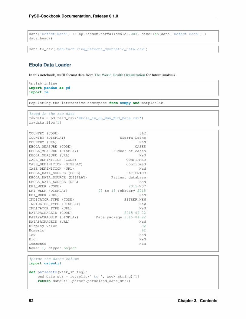
PySD-Cookbook Documentation, Release 0.1.0
data['Defect Rate'] += np.random.normal(scale=.003, size=len(data['Defect Rate']))data.head()
data.to_csv('Manufacturing_Defects_Synthetic_Data.csv')
Ebola Data Loader
In this notebook, we’ll format data from The World Health Organization for future analysis
%pylab inlineimport pandas as pdimport re
Populating the interactive namespace from numpy and matplotlib
#read in the raw datarawdata = pd.read_csv('Ebola_in_SL_Raw_WHO_Data.csv')rawdata.iloc[1]
COUNTRY (CODE) SLECOUNTRY (DISPLAY) Sierra LeoneCOUNTRY (URL) NaNEBOLA_MEASURE (CODE) CASESEBOLA_MEASURE (DISPLAY) Number of casesEBOLA_MEASURE (URL) NaNCASE_DEFINITION (CODE) CONFIRMEDCASE_DEFINITION (DISPLAY) ConfirmedCASE_DEFINITION (URL) NaNEBOLA_DATA_SOURCE (CODE) PATIENTDBEBOLA_DATA_SOURCE (DISPLAY) Patient databaseEBOLA_DATA_SOURCE (URL) NaNEPI_WEEK (CODE) 2015-W07EPI_WEEK (DISPLAY) 09 to 15 February 2015EPI_WEEK (URL) NaNINDICATOR_TYPE (CODE) SITREP_NEWINDICATOR_TYPE (DISPLAY) NewINDICATOR_TYPE (URL) NaNDATAPACKAGEID (CODE) 2015-04-22DATAPACKAGEID (DISPLAY) Data package 2015-04-22DATAPACKAGEID (URL) NaNDisplay Value 92Numeric 92Low NaNHigh NaNComments NaNName: 1, dtype: object
#parse the dates columnimport dateutil
def parsedate(week_string):end_date_str = re.split(' to ', week_string)[1]return(dateutil.parser.parse(end_date_str))
92 Chapter 3. Contents
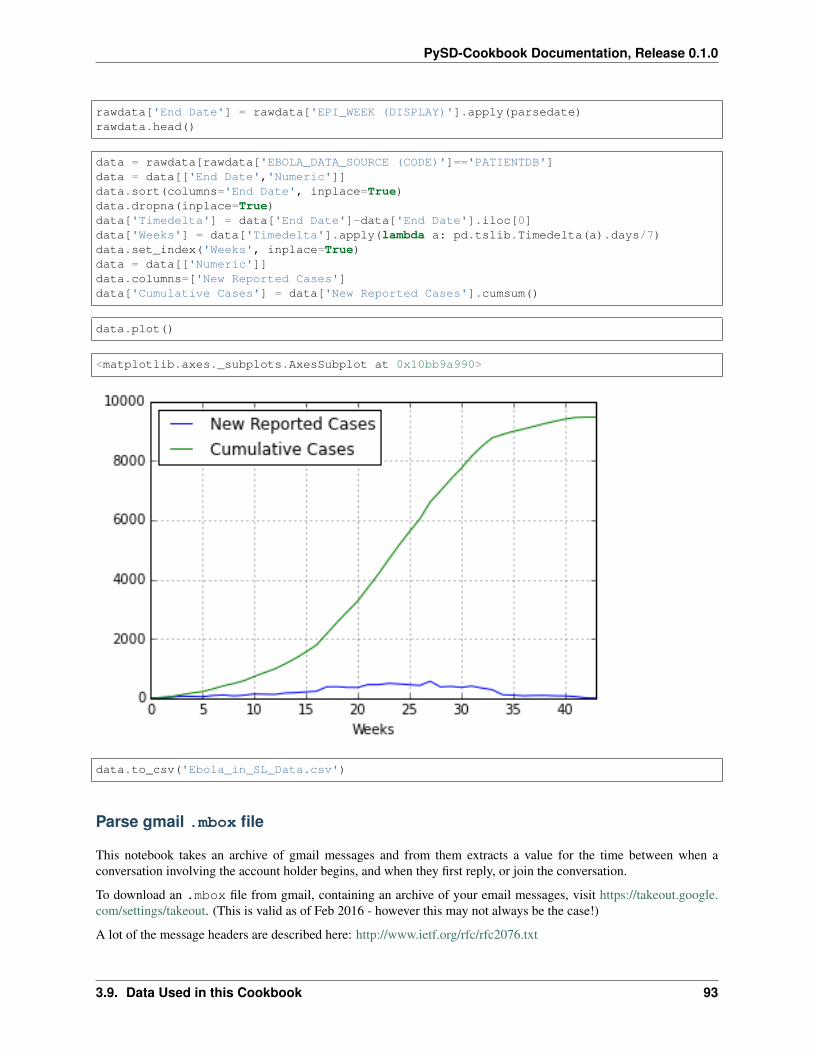
PySD-Cookbook Documentation, Release 0.1.0
rawdata['End Date'] = rawdata['EPI_WEEK (DISPLAY)'].apply(parsedate)rawdata.head()
data = rawdata[rawdata['EBOLA_DATA_SOURCE (CODE)']=='PATIENTDB']data = data[['End Date','Numeric']]data.sort(columns='End Date', inplace=True)data.dropna(inplace=True)data['Timedelta'] = data['End Date']-data['End Date'].iloc[0]data['Weeks'] = data['Timedelta'].apply(lambda a: pd.tslib.Timedelta(a).days/7)data.set_index('Weeks', inplace=True)data = data[['Numeric']]data.columns=['New Reported Cases']data['Cumulative Cases'] = data['New Reported Cases'].cumsum()
data.plot()
<matplotlib.axes._subplots.AxesSubplot at 0x10bb9a990>
data.to_csv('Ebola_in_SL_Data.csv')
Parse gmail .mbox file
This notebook takes an archive of gmail messages and from them extracts a value for the time between when aconversation involving the account holder begins, and when they first reply, or join the conversation.
To download an .mbox file from gmail, containing an archive of your email messages, visit https://takeout.google.com/settings/takeout. (This is valid as of Feb 2016 - however this may not always be the case!)
A lot of the message headers are described here: http://www.ietf.org/rfc/rfc2076.txt
3.9. Data Used in this Cookbook 93
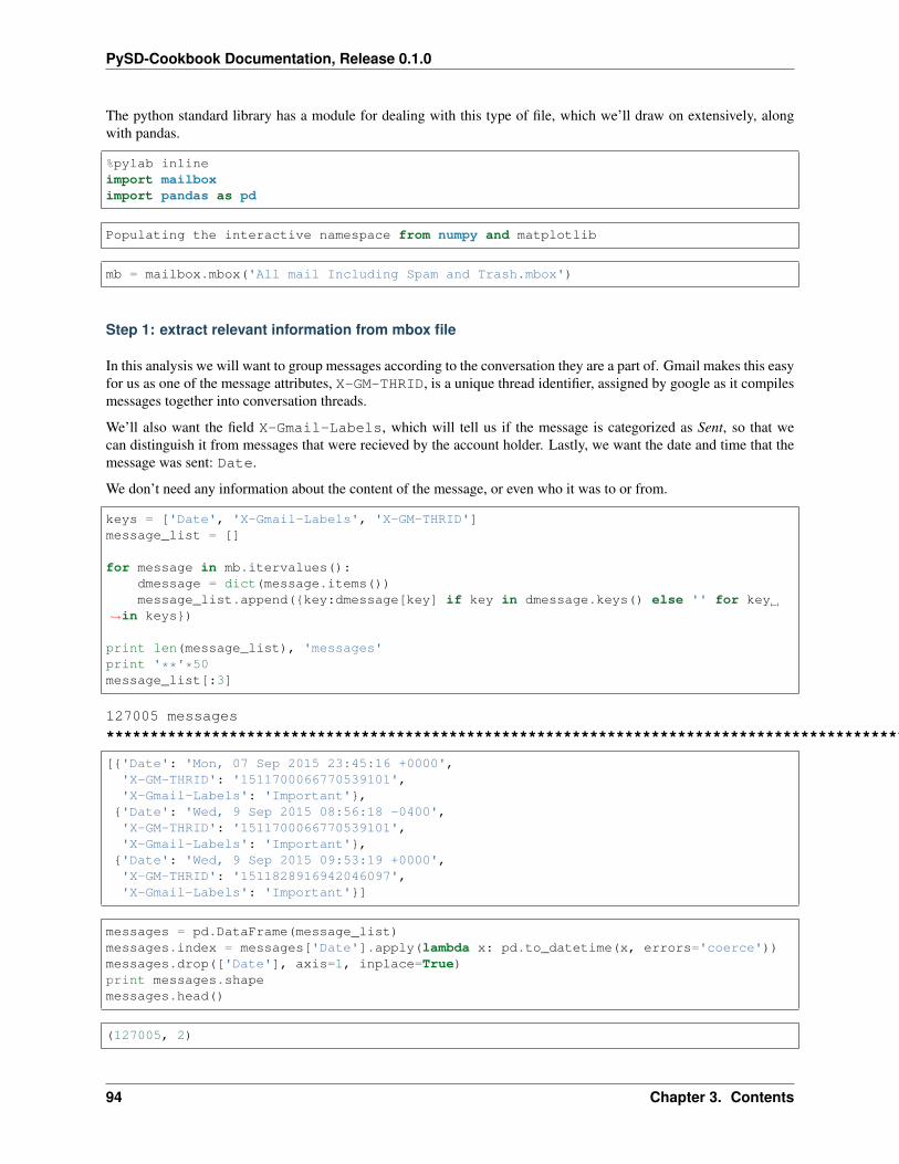
PySD-Cookbook Documentation, Release 0.1.0
The python standard library has a module for dealing with this type of file, which we’ll draw on extensively, alongwith pandas.
%pylab inlineimport mailboximport pandas as pd
Populating the interactive namespace from numpy and matplotlib
mb = mailbox.mbox('All mail Including Spam and Trash.mbox')
Step 1: extract relevant information from mbox file
In this analysis we will want to group messages according to the conversation they are a part of. Gmail makes this easyfor us as one of the message attributes, X-GM-THRID, is a unique thread identifier, assigned by google as it compilesmessages together into conversation threads.
We’ll also want the field X-Gmail-Labels, which will tell us if the message is categorized as Sent, so that wecan distinguish it from messages that were recieved by the account holder. Lastly, we want the date and time that themessage was sent: Date.
We don’t need any information about the content of the message, or even who it was to or from.
keys = ['Date', 'X-Gmail-Labels', 'X-GM-THRID']message_list = []
for message in mb.itervalues():dmessage = dict(message.items())message_list.append({key:dmessage[key] if key in dmessage.keys() else '' for key
→˓in keys})
print len(message_list), 'messages'print '**'*50message_list[:3]
127005 messages
************************************************************************************************
[{'Date': 'Mon, 07 Sep 2015 23:45:16 +0000','X-GM-THRID': '1511700066770539101','X-Gmail-Labels': 'Important'},
{'Date': 'Wed, 9 Sep 2015 08:56:18 -0400','X-GM-THRID': '1511700066770539101','X-Gmail-Labels': 'Important'},
{'Date': 'Wed, 9 Sep 2015 09:53:19 +0000','X-GM-THRID': '1511828916942046097','X-Gmail-Labels': 'Important'}]
messages = pd.DataFrame(message_list)messages.index = messages['Date'].apply(lambda x: pd.to_datetime(x, errors='coerce'))messages.drop(['Date'], axis=1, inplace=True)print messages.shapemessages.head()
(127005, 2)
94 Chapter 3. Contents
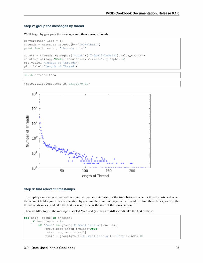
PySD-Cookbook Documentation, Release 0.1.0
Step 2: group the messages by thread
We’ll begin by grouping the messages into their various threads.
conversation_list = []threads = messages.groupby(by='X-GM-THRID')print len(threads), 'threads total'
counts = threads.aggregate('count')['X-Gmail-Labels'].value_counts()counts.plot(logy=True, linewidth=0, marker='.', alpha=.5)plt.ylabel('Number of Threads')plt.xlabel('Length of Thread')
32966 threads total
<matplotlib.text.Text at 0x10ca707d0>
Step 3: find relevant timestamps
To simplify our analysis, we will assume that we are interested in the time between when a thread starts and whenthe account holder joins the conversation by sending their first message in the thread. To find these times, we sort thethread on its index, and take the first message time as the start of the conversation.
Then we filter to just the messages labeled Sent, and (as they are still sorted) take the first of these.
for name, group in threads:if len(group) > 1:
if 'Sent' in group['X-Gmail-Labels'].values:group.sort_index(inplace=True)tstart = group.index[0]tjoin = group[group['X-Gmail-Labels']=='Sent'].index[0]
3.9. Data Used in this Cookbook 95
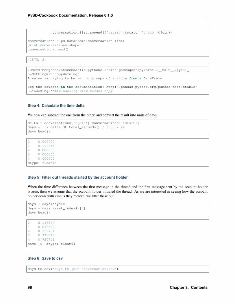
PySD-Cookbook Documentation, Release 0.1.0
conversation_list.append({'tstart':tstart, 'tjoin':tjoin})
conversations = pd.DataFrame(conversation_list)print conversations.shapeconversations.head()
(1873, 2)
/Users/houghton/anaconda/lib/python2.7/site-packages/ipykernel/__main__.py:4:→˓SettingWithCopyWarning:A value is trying to be set on a copy of a slice from a DataFrame
See the caveats in the documentation: http://pandas.pydata.org/pandas-docs/stable/→˓indexing.html#indexing-view-versus-copy
Step 4: Calculate the time delta
We now can subtract the one from the other, and convert the result into units of days.
delta = conversations['tjoin']-conversations['tstart']days = 1.* delta.dt.total_seconds() / 3600 / 24days.head()
0 0.0000001 0.1963542 0.0000003 0.0000004 0.000000dtype: float64
Step 5: Filter out threads started by the account holder
When the time difference between the first message in the thread and the first message sent by the account holderis zero, then we assume that the account holder initiated the thread. As we are interested in seeing how the accountholder deals with emails they recieve, we filter these out.
days = days[days>0]days = days.reset_index()[0]days.head()
0 0.1963541 0.0765392 0.3527313 0.3213434 0.720741Name: 0, dtype: float64
Step 6: Save to csv
days.to_csv('days_to_join_conversation.csv')
96 Chapter 3. Contents
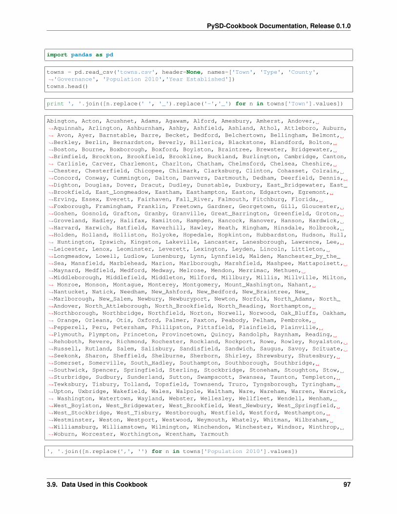
PySD-Cookbook Documentation, Release 0.1.0
import pandas as pd
towns = pd.read_csv('towns.csv', header=None, names=['Town', 'Type', 'County',→˓'Governance', 'Population 2010','Year Established'])towns.head()
print ', '.join([n.replace(' ', '_').replace('-','_') for n in towns['Town'].values])
Abington, Acton, Acushnet, Adams, Agawam, Alford, Amesbury, Amherst, Andover,→˓Aquinnah, Arlington, Ashburnham, Ashby, Ashfield, Ashland, Athol, Attleboro, Auburn,→˓ Avon, Ayer, Barnstable, Barre, Becket, Bedford, Belchertown, Bellingham, Belmont,→˓Berkley, Berlin, Bernardston, Beverly, Billerica, Blackstone, Blandford, Bolton,→˓Boston, Bourne, Boxborough, Boxford, Boylston, Braintree, Brewster, Bridgewater,→˓Brimfield, Brockton, Brookfield, Brookline, Buckland, Burlington, Cambridge, Canton,→˓ Carlisle, Carver, Charlemont, Charlton, Chatham, Chelmsford, Chelsea, Cheshire,→˓Chester, Chesterfield, Chicopee, Chilmark, Clarksburg, Clinton, Cohasset, Colrain,→˓Concord, Conway, Cummington, Dalton, Danvers, Dartmouth, Dedham, Deerfield, Dennis,→˓Dighton, Douglas, Dover, Dracut, Dudley, Dunstable, Duxbury, East_Bridgewater, East_→˓Brookfield, East_Longmeadow, Eastham, Easthampton, Easton, Edgartown, Egremont,→˓Erving, Essex, Everett, Fairhaven, Fall_River, Falmouth, Fitchburg, Florida,→˓Foxborough, Framingham, Franklin, Freetown, Gardner, Georgetown, Gill, Gloucester,→˓Goshen, Gosnold, Grafton, Granby, Granville, Great_Barrington, Greenfield, Groton,→˓Groveland, Hadley, Halifax, Hamilton, Hampden, Hancock, Hanover, Hanson, Hardwick,→˓Harvard, Harwich, Hatfield, Haverhill, Hawley, Heath, Hingham, Hinsdale, Holbrook,→˓Holden, Holland, Holliston, Holyoke, Hopedale, Hopkinton, Hubbardston, Hudson, Hull,→˓ Huntington, Ipswich, Kingston, Lakeville, Lancaster, Lanesborough, Lawrence, Lee,→˓Leicester, Lenox, Leominster, Leverett, Lexington, Leyden, Lincoln, Littleton,→˓Longmeadow, Lowell, Ludlow, Lunenburg, Lynn, Lynnfield, Malden, Manchester_by_the_→˓Sea, Mansfield, Marblehead, Marion, Marlborough, Marshfield, Mashpee, Mattapoisett,→˓Maynard, Medfield, Medford, Medway, Melrose, Mendon, Merrimac, Methuen,→˓Middleborough, Middlefield, Middleton, Milford, Millbury, Millis, Millville, Milton,→˓ Monroe, Monson, Montague, Monterey, Montgomery, Mount_Washington, Nahant,→˓Nantucket, Natick, Needham, New_Ashford, New_Bedford, New_Braintree, New_→˓Marlborough, New_Salem, Newbury, Newburyport, Newton, Norfolk, North_Adams, North_→˓Andover, North_Attleborough, North_Brookfield, North_Reading, Northampton,→˓Northborough, Northbridge, Northfield, Norton, Norwell, Norwood, Oak_Bluffs, Oakham,→˓ Orange, Orleans, Otis, Oxford, Palmer, Paxton, Peabody, Pelham, Pembroke,→˓Pepperell, Peru, Petersham, Phillipston, Pittsfield, Plainfield, Plainville,→˓Plymouth, Plympton, Princeton, Provincetown, Quincy, Randolph, Raynham, Reading,→˓Rehoboth, Revere, Richmond, Rochester, Rockland, Rockport, Rowe, Rowley, Royalston,→˓Russell, Rutland, Salem, Salisbury, Sandisfield, Sandwich, Saugus, Savoy, Scituate,→˓Seekonk, Sharon, Sheffield, Shelburne, Sherborn, Shirley, Shrewsbury, Shutesbury,→˓Somerset, Somerville, South_Hadley, Southampton, Southborough, Southbridge,→˓Southwick, Spencer, Springfield, Sterling, Stockbridge, Stoneham, Stoughton, Stow,→˓Sturbridge, Sudbury, Sunderland, Sutton, Swampscott, Swansea, Taunton, Templeton,→˓Tewksbury, Tisbury, Tolland, Topsfield, Townsend, Truro, Tyngsborough, Tyringham,→˓Upton, Uxbridge, Wakefield, Wales, Walpole, Waltham, Ware, Wareham, Warren, Warwick,→˓ Washington, Watertown, Wayland, Webster, Wellesley, Wellfleet, Wendell, Wenham,→˓West_Boylston, West_Bridgewater, West_Brookfield, West_Newbury, West_Springfield,→˓West_Stockbridge, West_Tisbury, Westborough, Westfield, Westford, Westhampton,→˓Westminster, Weston, Westport, Westwood, Weymouth, Whately, Whitman, Wilbraham,→˓Williamsburg, Williamstown, Wilmington, Winchendon, Winchester, Windsor, Winthrop,→˓Woburn, Worcester, Worthington, Wrentham, Yarmouth
', '.join([n.replace(',', '') for n in towns['Population 2010'].values])
3.9. Data Used in this Cookbook 97
PySD-Cookbook Documentation, Release 0.1.0
'15985, 21924, 10303, 8485, 28438, 494, 16283, 37819, 33201, 311, 42844, 6081, 3074,→˓1737, 16593, 11584, 43593, 16188, 4356, 7427, 45193, 5398, 1779, 13320, 14649,→˓16332, 24729, 6411, 2866, 2129, 39502, 40243, 9026, 1233, 4897, 617660, 19754, 4996,→˓ 7965, 4355, 35744, 9820, 26563, 3609, 93810, 3390, 58732, 1902, 24498, 105162,→˓21561, 4852, 11509, 1266, 12981, 6125, 33802, 35177, 3235, 1337, 1222, 55298, 866,→˓1702, 13606, 7542, 1671, 17668, 1897, 872, 6756, 26493, 34032, 24729, 5125, 14207,→˓7086, 8471, 5589, 29457, 11390, 3179, 15059, 13794, 2183, 15720, 4956, 16053, 23112,→˓ 4067, 1225, 1800, 3504, 41667, 15873, 88857, 31531, 40318, 752, 16865, 68318,→˓31635, 8870, 20228, 8183, 1500, 28789, 1054, 75, 17765, 6240, 1566, 7104, 17456,→˓10646, 6459, 5250, 7518, 7764, 5139, 717, 13879, 10209, 2990, 6520, 12243, 3279,→˓60879, 337, 706, 22157, 2032, 10791, 17346, 2481, 13547, 39880, 5911, 14925, 4382,→˓19063, 10293, 2180, 13175, 12629, 10602, 8055, 3091, 76377, 5943, 10970, 5025,→˓40759, 1851, 31394, 711, 6362, 8924, 15784, 106519, 21103, 10086, 90329, 11596,→˓59450, 5136, 23184, 19808, 4907, 38499, 25132, 14006, 6045, 10106, 12024, 56173,→˓12752, 26983, 5839, 6338, 47255, 23116, 521, 8987, 27999, 13261, 7891, 3190, 27003,→˓121, 8560, 8437, 961, 838, 167, 3410, 10172, 33006, 28886, 228, 95072, 999, 1509,→˓990, 6666, 17416, 85146, 11227, 13708, 28352, 28712, 4680, 14892, 28549, 14155,→˓15707, 3032, 19031, 10506, 28602, 4527, 1902, 7839, 5890, 1612, 13709, 12140, 4806,→˓51251, 1321, 17837, 11497, 847, 1234, 1682, 44737, 648, 8264, 56468, 2820, 3413,→˓2942, 92271, 32112, 13383, 24747, 11608, 51755, 1475, 5232, 17489, 6952, 393, 5856,→˓1258, 1775, 7973, 41340, 8283, 915, 20675, 26628, 692, 18133, 13722, 17612, 3257,→˓1893, 4119, 7211, 35608, 1771, 18165, 75754, 17514, 5792, 9767, 16719, 9502, 11688,→˓153060, 7808, 1947, 21437, 26962, 6590, 9268, 17659, 3684, 8963, 13787, 15865,→˓55874, 8013, 28961, 3949, 485, 6085, 8926, 2003, 11292, 327, 7542, 13457, 24932,→˓1838, 24070, 60632, 9872, 21822, 5135, 780, 538, 31915, 12994, 16767, 27982, 2750,→˓848, 4875, 7669, 6916, 3701, 4235, 28391, 1306, 2740, 18272, 41094, 21951, 1607,→˓7277, 11261, 15532, 14618, 53743, 1496, 14489, 14219, 2482, 7754, 22325, 10300,→˓21374, 899, 17497, 38120, 181045, 1156, 10955, 23793'
Chapters to be Written
This cookbook is a work in progress. In the future, I’d like to develop examples in the following major areas. If you’dlike to suggest additional topics, or have a model and/or dataset that would make for a good case study, feel free toshoot me an email ([email protected]) or post on the Github issue tracker.
This is a notional listing of desired chapters, with existing chapters
1. Model Fitting to data
(a) optimizing in the phase space
(b) Frequency Domain
(c) Fitting to multiple datasets
(d) Fitting with unobserved states/ unobserved stocks
2. Monte Carlo Analysis
(a) Sensitivity Analysis
(b) Propagation of Uncertainties
3. Markov Chain Monte Carlo
(a) Estimating parameter distributions for a single model
(b) Reversible jump MCMC for model selection
4. Working with geographic data
98 Chapter 3. Contents
PySD-Cookbook Documentation, Release 0.1.0
5. Patch Models
6. Linking models together
7. Surrogating model functions with data
(a) Nearest neighbors methods
8. Plotting and displaying simulation output
(a) Static Visualization
(b) Interactive Plots
9. Driving a model with external data
10. Loading and processing data in real time
11. Kalman filtering on realtime data
12. Multiple Models
13. Clustering model outputs
1. based upon timeseries features
2. based upon derivative features
3. based upon phase-plane features
4. based upon estimated(fit) parameters
14. Bootstrapping/cross validations
1. Multiple datasets
2. Partitioned timeseriese
15. Statistical screening
1. Screening for sensitivity analysis
16. Hidden markov models and dynamic models
17. Machine Learning predictors and dynamic models
18. Testing policy robustness
19. Extreme conditions testing - unit testing on models.
20. Pysd and Exploratory Modeling Analysis Workbench
End Notes
For instruction
The notebooks in this cookbook can be used as slide decks. To do so, install the rise package.
3.11. End Notes 99

PySD-Cookbook Documentation, Release 0.1.0
100 Chapter 3. Contents
CHAPTER 4
Extra Resources
The PySD Documentation can answer most questions about how PySD itself should be used, with basic examples andfunction reference.
101

PySD-Cookbook Documentation, Release 0.1.0
102 Chapter 4. Extra Resources
CHAPTER 5
Indices and tables
• genindex
• modindex
• search
103