python based 4d visualization environment · python based 4d visualization environment 1lin jing,...

Python based 4D Visualization Environment

1Lin Jing, 1Xipei Huang, 1Yiwen Zhong, 2Yin Wu, *3Hui Zhang 1, First Author College of Computer and Information Science, Fujian Agriculture and Forestry

University, Fuzhou, China, [email protected] 2 School of Informatics and Computing, Indiana University, Bloomington, USA

*3, Corresponding Author Pervasive Technology Institute, Indiana University, Indianapolis, USA, [email protected]

Abstract

One of the challenges in 4D math visualization is to develop an interactive and integrated computational environment to quick-prototype, simulate, and experiment with the abstract mathematical concepts. We have investigated several areas in 4D visualization, including 4D surface rendering, various user interface elements to manipulate mathematical objects in the higher-dimensional space, and physically based modeling of cloth-like 4D objects to understand the math phenomena in the fourth dimension. In this paper, we present one such Python based 4D visualization environment that achieves a high level of integration between 4D math, physics computation and interactive visualization. Several examples are given in this paper to show how various math phenomena can be simulated in our software environment to enhance our understanding of the fourth dimension.

Keywords: Math Visualization, 4D Visualization, Python 1. Introduction

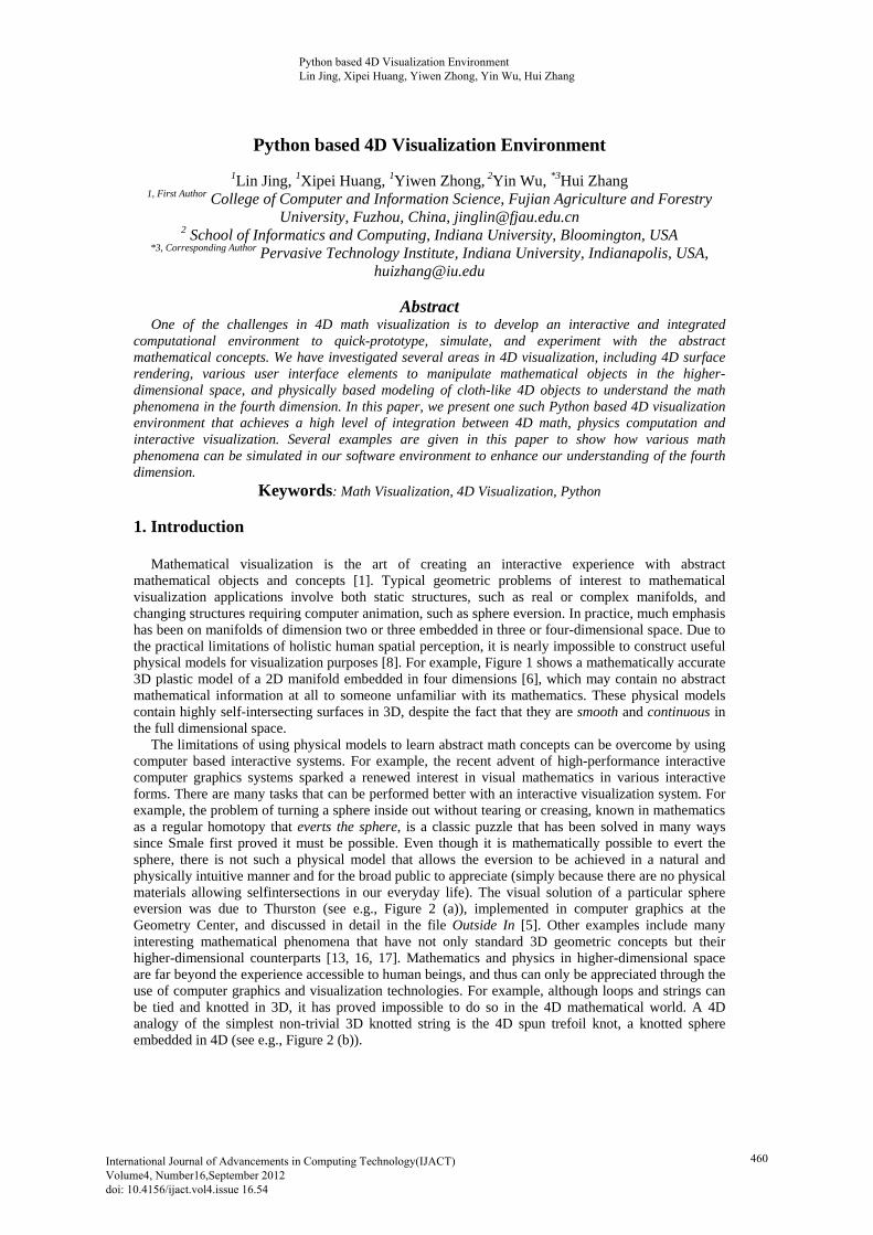
Mathematical visualization is the art of creating an interactive experience with abstract mathematical objects and concepts [1]. Typical geometric problems of interest to mathematical visualization applications involve both static structures, such as real or complex manifolds, and changing structures requiring computer animation, such as sphere eversion. In practice, much emphasis has been on manifolds of dimension two or three embedded in three or four-dimensional space. Due to the practical limitations of holistic human spatial perception, it is nearly impossible to construct useful physical models for visualization purposes [8]. For example, Figure 1 shows a mathematically accurate 3D plastic model of a 2D manifold embedded in four dimensions [6], which may contain no abstract mathematical information at all to someone unfamiliar with its mathematics. These physical models contain highly self-intersecting surfaces in 3D, despite the fact that they are smooth and continuous in the full dimensional space.

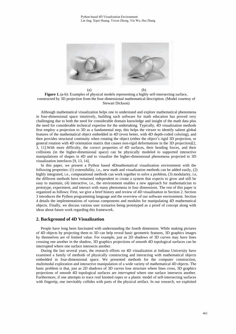
The limitations of using physical models to learn abstract math concepts can be overcome by using computer based interactive systems. For example, the recent advent of high-performance interactive computer graphics systems sparked a renewed interest in visual mathematics in various interactive forms. There are many tasks that can be performed better with an interactive visualization system. For example, the problem of turning a sphere inside out without tearing or creasing, known in mathematics as a regular homotopy that everts the sphere, is a classic puzzle that has been solved in many ways since Smale first proved it must be possible. Even though it is mathematically possible to evert the sphere, there is not such a physical model that allows the eversion to be achieved in a natural and physically intuitive manner and for the broad public to appreciate (simply because there are no physical materials allowing selfintersections in our everyday life). The visual solution of a particular sphere eversion was due to Thurston (see e.g., Figure 2 (a)), implemented in computer graphics at the Geometry Center, and discussed in detail in the file Outside In [5]. Other examples include many interesting mathematical phenomena that have not only standard 3D geometric concepts but their higher-dimensional counterparts [13, 16, 17]. Mathematics and physics in higher-dimensional space are far beyond the experience accessible to human beings, and thus can only be appreciated through the use of computer graphics and visualization technologies. For example, although loops and strings can be tied and knotted in 3D, it has proved impossible to do so in the 4D mathematical world. A 4D analogy of the simplest non-trivial 3D knotted string is the 4D spun trefoil knot, a knotted sphere embedded in 4D (see e.g., Figure 2 (b)).

Python based 4D Visualization Environment Lin Jing, Xipei Huang, Yiwen Zhong, Yin Wu, Hui Zhang

International Journal of Advancements in Computing Technology(IJACT) Volume4, Number16,September 2012 doi: 10.4156/ijact.vol4.issue 16.54

460

(a) (b)

Figure 1. (a-b): Examples of physical models representing a highly self-intersecting surface, constructed by 3D projection from the four-dimensional mathematical description. (Model courtesy of

Stewart Dickson)

Although mathematical visualization helps one to understand and explore mathematical phenomena in four-dimensional space intuitively, building such software for math education has proved very challenging due to both the need for considerable domain knowledge and insight of the math data plus the need for considerable technical expertise for the undertaking. Typically, 4D visualization methods first employ a projection to 3D as a fundamental step; this helps the viewer to identify salient global features of the mathematical object embedded in 4D (even better, with 4D depth-coded coloring), and then provides structural continuity when rotating the object (either the object’s rigid 3D projection, or general rotation with 4D orientation matrix that causes non-rigid deformations in the 3D projection)[2, 3, 11].With more difficulty, the correct properties of 4D surfaces, their bending forces, and their collisions (in the higher-dimensional space) can be physically modeled to supported interactive manipulations of shapes in 4D and to visualize the higher-dimensional phenomena projected to 3D visualization interfaces [9, 13, 14].

In this paper, we present a Python based 4Dmathematical visualization environment with the following properties: (1) extensibility, i.e., new math and visualization methods can be added easily, (2) highly integrated, i.e., computational methods can work together to solve a problem, (3) modularity, i.e, the different methods have remained independent to create a system that expects to grow and still be easy to maintain, (4) interactive, i.e., the environment enables a new approach for mathematician to prototype, experiment, and interact with many phenomena in four dimensions. The rest of this paper is organized as follows: First, we give a brief history and review of 4D visualization in Section 2. Section 3 introduces the Python programming language and the overview of our software environment. Section 4 details the implementations of various components and modules for manipulating 4D mathematical objects. Finally, we discuss various user scenarios being prototyped as a proof of concept along with ideas about future work regarding this framework.

2. Background of 4D Visualization

People have long been fascinated with understanding the fourth dimension. While making pictures of 4D objects by projecting them to 3D can help reveal basic geometric features, 3D graphics images by themselves are of limited value. For example, just as 2D shadows of 3D curves may have lines crossing one another in the shadow, 3D graphics projections of smooth 4D topological surfaces can be interrupted where one surface intersects another.

During the last several years, the research efforts on 4D visualization at Indiana University have examined a family of methods of physically constructing and interacting with mathematical objects embedded in four-dimensional space. We presented methods for the computer construction, multimodal exploration and interactive manipulation of a wide variety of mathematical 4D objects. The basic problem is that, just as 2D shadows of 3D curves lose structure where lines cross, 3D graphics projections of smooth 4D topological surfaces are interrupted where one surface intersects another. Furthermore, if one attempts to trace real knotted ropes or a plastic model of self-intersecting surfaces with fingertip, one inevitably collides with parts of the physical artifact. In our research, we exploited


461

the free motion of a computer-based haptic probe to support a continuous motion that follows the local continuity of the object being explored. The proposed haptics techniques to explore mathematic objects in 4D have also led to a new interaction technique without a real haptic interface. The real haptic interface can be replaced by adaptive motion of the mouse cursor on the computer screen, e.g., slowing the response to simulate collision [15].

(a) (b)

Figure 2. (a) Thurstons method for everting the sphere. (b) A rendered 3D image of 4D spun trefoilknot, the 4D analogy of 3D trefoil knot.

By combining graphics and various interaction techniques, we have found a way to enhance our

experience of interacting with 4D object by producing a reduced-dimension 3D tool for manipulating objects embedded in 4D. By physically modeling the correct properties of 4D surfaces, their bending forces, and their collisions in the 3D haptic controller interface, we can support full-featured computer-based exploration of 4D mathematical objects in a manner that is otherwise far beyond the experience accessible to human beings. 3. A Python based 4D Visualization Environment

Different from many other general graphics applications, 4D math visualization systems as such often require customized hybrid approaches and there are a number of considerations when choosing a platform or language for the undertaking. For example, the undertaking usually spans several fields including computer based visualization, graphics, numerical computation, and physically based modeling. In our experiments, we have had very good success using Python. Python is a very high-level, interpreted language that is perfect for mathematician’s quick experimentation and rapid prototyping. A number of freely available contributed libraries for Python make it a wonderful platform language for 4D visualization [12]: Math and Physics aware: Numerical libraries (i.e., ScientificPython, NumPy and SciPy) have

added array and matrix support to the Python language. High-performance numerical routines, matrix and multidimensional array operations, optimizations, and linear algebra are now seamlessly achievable with Python.

Graphics-supporting: OpenGL package and VPython module allow access to the underlying graphics hardware for fast 3D rendering, and easy creations of navigable 3D scene graph and animation (even for those with limited programming experience).

Interactive: Python is designed for quick experimentation and rapid prototyping. This is one of key facets we are looking for when building math visualization environment.

Open environment: Python is open source, easy-to-integrate, and therefore able to interact with many other tools. As shown in Figure 3, our 4D visualization environment is based on a wide of varieties of

contributed libraries developed on Python. In the next section, we will describe the families of modules we developed to manipulate and render the projected images of mathematical objects embedded in four dimensions.


462

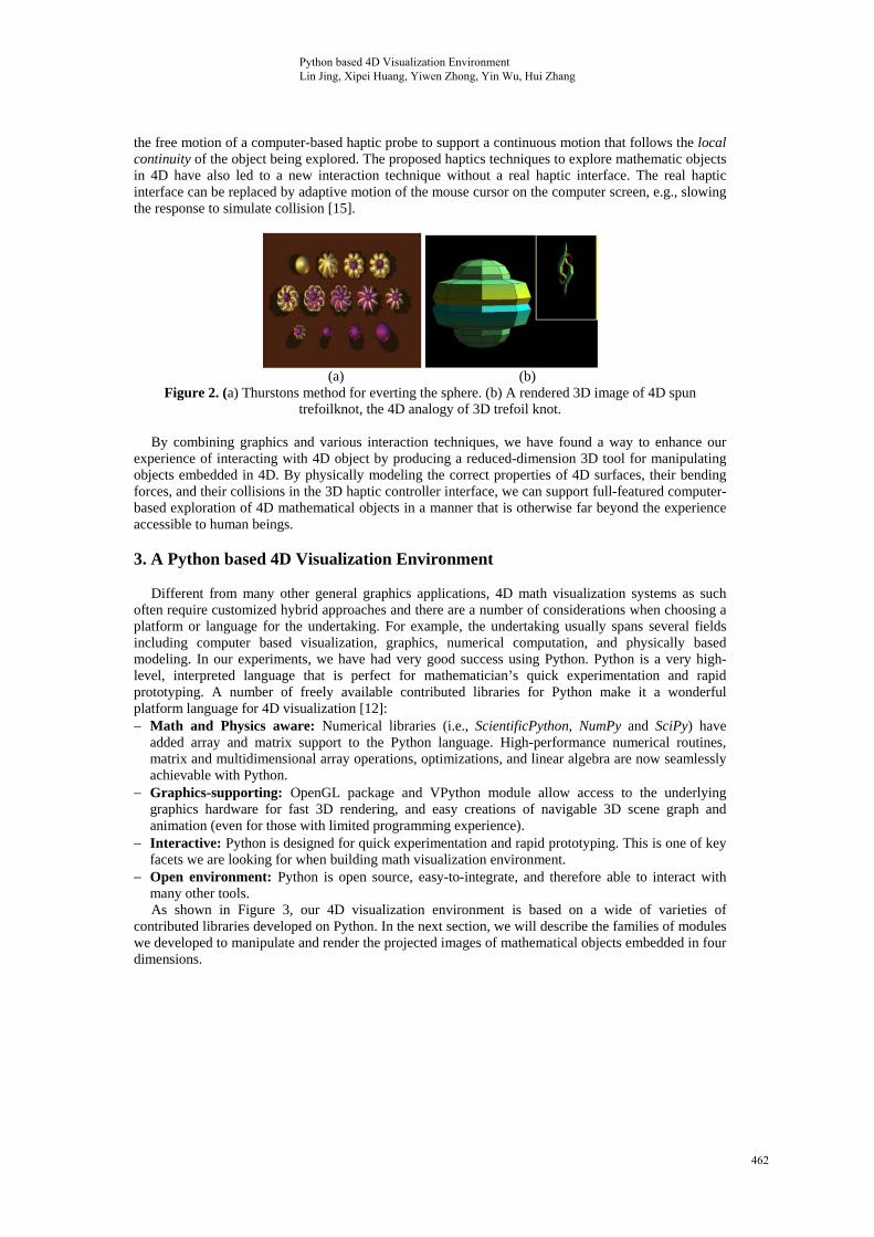
Figure 3. Architecture and Modules Overview of our 4D Visualization System.

4. Implementation methods and modules 4.1. Geom4D module

The Geom4D module provides a family of 4D vector operations and distance computation functions in Vect4D class. The Poly4D class defines the data structure of 4D polygonal model composed of points, lines, and polygons embedded in four dimensions, and provides useful interfaces to construct 4D objects by loading the OOGL (object Oriented Graphics Language) file format, such as MESH, OFF files.

Vector Operations and Points in 4D For the most part, vector operations in four space are simple extensions of their three-space counterparts. For example, computing the addition of two four-vectors is a matter of forming a resultant vector whose components are the pairwise sums of the coordinates of the two operand vectors. In the same fashion, subtraction, scaling, and dot-products are all simple extensions of their more common three-vector counterparts.

In addition, operations between four-space points and vectors are also simple extensions of the more common three-space points and vectors. For example, computing the four-vector difference of four-space points is a simple matter of subtracting pairwise coordinates of the two points to yield the four coordinates of the resulting four-vector.

For completeness, the equations of the more common four-space vector operations follow. In these equations, 0 1 2 3, , ,U U U U U and 3210 ,,, VVVVV are two source four-vectors and k is a scalar value:

33221100

3210

33221100

33221100

,,,

,,,

,,,

,,,

VUVUVUVUVU

kUkUkUkUkU

VUVUVUVUVU

VUVUVUVUVU

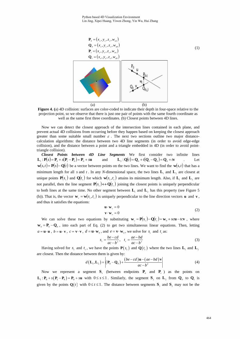
Distances in 4D To understand the non-intuitive mechanisms of 4D collision, let us start with a pair of two-dimensional planes through the origin in four-dimensional space (see Figure 4). The two squares intersect in a single 4D point at the origin. In the three dimensional projection, although the planes appear to intersect along an entire line due to the annihilation of the w dimension, when the surfaces are 4D depth color-coded, we can see that there is just one pair of points with the same fourth coordinates as well as the same coordinates in the 3D projection. Note that 4D collisions take place only if there is also a 3D collision in the shadow, but that 3D shadow collisions may not imply 4D collisions.

Figure 4 (b) illustrates the basic case for 4D collision detection; a 4D depth collision test must be performed along the intersecting lines of the projected images of 4D surfaces. 4D collision occurs if, and only if, one or more pairs of points are located with same fourth coordinate along the intersecting line. Now let 4D surfaces AS and BS intersect in the 3D projected image along the line segment seL ,

from point ssss zvx ,,P to point eeee zyx ,,P . Suppose the pair of 4D points sharing sP as

shadow points are 0P on AS , and 0Q on BS ; likewise, we have 1P on AS , and 1Q on BS sharing eP

as shadow point. Obviously, 0P , 1P , 0Q , and 1Q can be represented as:


463

eBeee

eAeee

sBsss

sAsss

wzyx

wzyx

wzyx

wzyx

,,,

,,,

,,,

,,,

1

1

0

0

Q

P

Q

P

(1)

(a) (b)

Figure 4. (a) 4D collision: surfaces are color-coded to indicate their depth in four-space relative to the projection point, so we observe that there is just one pair of points with the same fourth coordinate as

well as the same first three coordinates. (b) Closest points between 4D lines.

Now we can detect the closest approach of the intersection lines contained in each plane, and prevent actual 4D collisions from occurring before they happen based on keeping the closest approach greater than some suitable small number . The next two sections outline two major distance-calculation algorithms: the distance between two 4D line segments (in order to avoid edge-edge collision), and the distance between a point and a triangle embedded in 4D (in order to avoid point-triangle collision).

Closest Points between 4D Line Segments We first consider two infinite lines uPPPPPL sss 00101 : and vQQQQQL ttt 00102 : . Let

tsts QPw , be a vector between points on the two lines. We want to find the ts,w that has a

minimum length for all s and t . In any N-dimensional space, the two lines 1L and 2L are closest at

unique points csP and ctQ for which cc ts ,w attains its minimum length. Also, if 1L and 2L are

not parallel, then the line segment cc ts QP joining the closest points is uniquely perpendicular

to both lines at the same time. No other segment between 1L and 2L has this property (see Figure 5

(b)). That is, the vector ccc ts ,ww is uniquely perpendicular to the line direction vectors u and v ,

and thus it satisfies the equations:

0

0

c

c

wv

wu (2)

We can solve these two equations by substituting vuwQPw tcscts ccc 0 , where

000 QPw , into each part of Eq. (2) to get two simultaneous linear equations. Then, letting

uu a , vu b , vv c , 0wu d , and 0wv e , we solve for cs and ct as:

22,

bac

bdaet

bac

cdbes cc

(3)

Having solved for cs and ct , we have the points csP and ctQ where the two lines 1L and 2L

are closest. Then the distance between them is given by:

1 2 0 0 2,

be cd ae bdd

ac b

u v

L L P Q (4)

Now we represent a segment 1S (between endpoints 0P and 1P ) as the points on

1 0 1 0 0: s s L P P P P u with 10 s . Similarly, the segment 2S on 2L from 0Q to 1Q is

given by the points tQ with 10 t . The distance between segments 1S and 2S may not be the


464

same as the distance between their extended lines 1L and 2L . The first step in computing a distance

involving segments is to get the closest points for the lines they lie on. So, we first compute cs and ct

for 1L and 2L , and if these are in the range of the involved segment, then they are also the closest

points for them. But if they lie outside the range, then they are not and we have to determine new points that minimize ,s t s t W P Q over the ranges of interest.

To do this, we first note that minimizing the length of w is the same as minimizing

0 0| | s t s t W W W W u v W u v which is a quadratic function of s and t . In fact, this

expression defines a paraboloid over the ts, -plane with a minimum at cc tsC , , and which is

strictly increasing along rays in the ts, -plane that start from C and go in any direction. However,

when segments are involved, we need the minimum over a subregion G of the ts, -plane, and the

global minimum at C may lie outside of G . An approach is given by [4], suggesting that the minimum always occurs on the boundary of G , and in particular, on the part of s'G boundary that is visible to C . Thus by testing all candidate boundaries, we can compute the closest points between 4D line segments.

Closest Points between 4D Point and Triangle The problem now is to compute the minimum distance between a point P and a triangle 10, EEBT tsts for Dts , ,

1,1,0,1,0:, tststsD . The minimum distance is computed by locating the value Dts ,

corresponding to the point on the triangle closest to P . Note that our algorithm should work also for a triangle and a point embedded in arbitrary dimensions.

The squared-distance function for any point on the triangle to P is 2|,|, PT tstsQ for

Dts , . The function is quadratic in s and t ,

fetdsctbstastsQ 222, 22 , (5)

where 00 EE a , 10 EE b , 11 EE c , PBE 0d , PBE 1e , and PBPB f .

Quadratics are classified by the sign of 2bac , which here becomes

0|| 2

10

2

101100

2 EEEEEEEEbac (6)

The positivity is based on the assumption that the two edges 0E and 1E of the triangle are linearly

independent, so their cross product is a nonzero vector. In calculus terms, the goal is to minimize tsQ , over D . Since Q is a continuously differentiable function, the minimum occurs either at an

interior point of D where the gradient 0,0,2 ectbsdbtasQ , or at a point on the

boundary of D .

The Algorithm The gradient of Q is zero only when 2baccdbes and

2bacaebdt . If Dts , , then we have found the minimum of Q . Otherwise, the minimum

must occur on the boundary of the triangle. To find the correct boundary, consider Figure 7 (a).

The central triangle labeled region 0 is the domain of DtsQ , . If ts, is in region 0, then the

point on the triangle closest to P is interior to the triangle.

Suppose ts, is in region 1. The level curves of Q are those curves in the st -plane for which Q

is a constant. Since the graph of Q is a paraboloid, the level curves are ellipses. At the point where

0,0Q , the level curve degenerates to a single point ts, . The global minimum of Q occurs

there, call it minV . As the level values V increase from minV , the corresponding ellipses are increasingly

further away from ts, . There is a smallest level value 0V for which the corresponding ellipses are

increasingly further away from ts, . There is a smallest level value 0V for which the corresponding

ellipse (implicitly defined by 0VQ just touches the triangle domain edge 1 ts at a value

1,00 ss , 00 1 st . For level values 0VV , the corresponding ellipses do not intersect D . For

level values 0VV , portions of D lie inside the corresponding ellipses.


465

4.2. Phy4D module

In Phy4D module, we provide a library to model 4D surfaces with a 4D mass-spring system supporting physical interaction. In practice, we focus on 2-manifold deformable objects embedded in 4D. The Phy4D module extends the 3D mass-spring system to four dimensions, as can be used to model the 4D mathematical and physical behavior of 4D topological surfaces.

When applying the 4D mass-spring system to 2-manifold deformable objects, we assume that each mass point i is linked to all the others with (linear) springs of rest length 0

, jil and stiffness jik , . This

stiffness is set to zero if the actual model does not contain a spring between mass i and j . The

following three types of linear springs are used in our 4D interactive system: springs linking masses ji, and ji ,1 , and masses ji, and 1, ji , will be referred to as

“structural springs”; springs linking masses ji, and 1,1 ji , and masses ji ,1 and 1, ji , will be referred to

as “shear springs”; springs linking masses ji, and 1,2 ji , and masses ji, and 2, ji , will be referred to as

“bending springs”; 4.3. UI4D module

The family of user interface elements is provided in the UI4Dmodule, among them we note the 4D rotation, shadow based editing method, and 4D surface rendering method.

4D Rotation Rotation in four-space is initially difficult to conceive because the first impulse is to try to rotate about an axis in four-space. Rotation about an axis is an idea fostered by our experience in three-space, but it is only coincidence that any rotation in three-space can be determined by an axis in three-space.

For example, consider the idea of rotation in two-space. The axis that we rotate “about” is perpendicular to this space; it isn’t even contained in the two-space. In addition, given an origin of rotation and a fixed axis in three-space, the set of all rotated points for a given rotation matrix lie in a single plane, just like the two-space case.

Rotations in four-space are more properly thought of not as rotations about an axis, but as rotations about a 2D plane. This way of thinking about rotations is consistent with both two-space (where there is only one such plane) and three-space (where each rotation “axis” defines a unique rotation plane perpendicular to the normal vector to that plane).

Once this idea is established, it is easy to construct the basis for 4D rotation matrices, since only two coordinates will change for a given rotation. There are six 4D basis rotation matrices, corresponding to the YWXWZXYZXY ,,,, and ZW planes. There are given by (using angle ):

cossin00

sincos00

0010

0001

cos0sin0

0100

sin0cos0

0001

cos00sin

0100

0010

sin00cos1000

0cos0sin

0010

0sin0cos

1000

0cossin0

0sincos0

0001

1000

0100

00cossin

00sincos

zwywxw

zxyzxy

RRR

RRR

In this module, a separate mouse-driven orientation control is provided to adjust the 4D rotation matrix whose first two columns define the projection plane; this allows sufficient control to achieve a good projection for each particular editing subtask.

Shadow Editing Picking and selecting is provided in the UI4D module. Once a control point is selected, forces can be applied in the projected space. By combining general 4D rotations and virtual forces in the projected 3D space, users can interact with mathematical objects embedded in 4D [13].

Rendering UI4D module also provides an interface between the mathematical objects in 4D and the visual components in VPython module. Wrap-up functions are provided for rendering 4D objects (points, lines, polygons, and manifolds embedded in 4D) projected to 3D space.

Our 4D visualization environment can be used to develop a correct interactive experience with the


466

intuitive nature of unfamiliar 4D geometry. One value of our 4D visualization environment is that by zeroing sub-dimensions in the 4D mass-spring system, we can also simulate mathematical and physical phenomena in 2D and 3D, using deformable curves and manifolds in 2D and 3D. This makes it possible for mathematicians to prototype and experiment with dimensional progress analogies. Some of such examples are as follows.

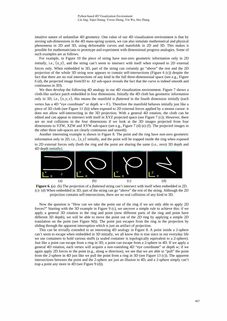
For example, in Figure 10 the piece of string have non-zero geometric information only in 2D initially, i.e., yx, , and the string can’t seem to intersect with itself when exposed to 2D external

forces only. When embedded in 3D, part of the string can certainly go “above” the rest and the 2D projection of the whole 3D string now appears to contain self-intersections (Figure 6 (c)) despite the fact that there are no real intersections of any kind in the full three-dimensional space (see e.g., Figure 6 (d), the projected image from3D to XZ sub-space reveals the fact that the curve is indeed smooth and continuous in 3D).

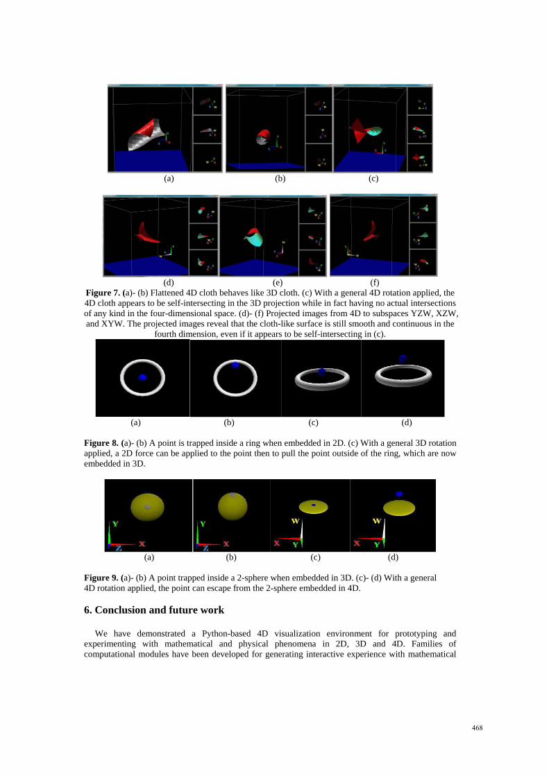
We then develop the following 4D analogy in our 4D visualization environment. Figure 7 shows a cloth-like surface patch embedded in four dimensions. Initially the 4D cloth has geometric information only in 3D, i.e., zyx ,, , this means the manifold is flattened in the fourth dimension initially (each

vertex has a 4D “eye coordinate” or depth 0w ). Therefore the manifold behaves initially just like a piece of 3D cloth (see Figure 11 (b)) when exposed to 2D external forces applied by a mouse cursor: it does not allow self-intersecting in the 3D projection. With a general 4D rotation, the cloth can be edited and can appear to intersect with itself in XYZ projected space (see Figure 7 (c)). However, there are no real collisions in the four dimensions if we look at the 3D images projected from four dimensions to YZW, XZW and XYW sub-space (see e.g., Figure 7 (d) (e) (f). The projected images in the other three sub-spaces are clearly continuous and smooth).

Another interesting example is shown in Figure 8. The point and the ring have non-zero geometric information only in 2D, i.e., yx, initially, and the point will be trapped inside the ring when exposed

to 2D external forces only (both the ring and the point are sharing the same (i.e., zero) 3D depth and 4D depth initially).

(a) (b) (c) (d)

Figure 6. (a)- (b) The projection of a flattened string can’t intersect with itself when embedded in 2D. (c)- (d) When embedded in 3D, part of the string can go “above” the rest of the string. Although the 2D

projection contains self-intersections, there are no real collisions of any kind in 3D.

Now the question is “How can we take the point out of the ring if we are only able to apply 2D

forces?” Starting with the 3D example in Figure 9 (c), we uncover a simple rule to achieve this: if we apply a general 3D rotation to the ring and point (now different parts of the ring and point have different 3D depth), we will be able to move the point out of the 2D ring by applying a simple 2D translation on the point (see Figure 9d)). The point just escapes from the ring in the projection by sliding through the apparent interruption which is just an artifact of projection.

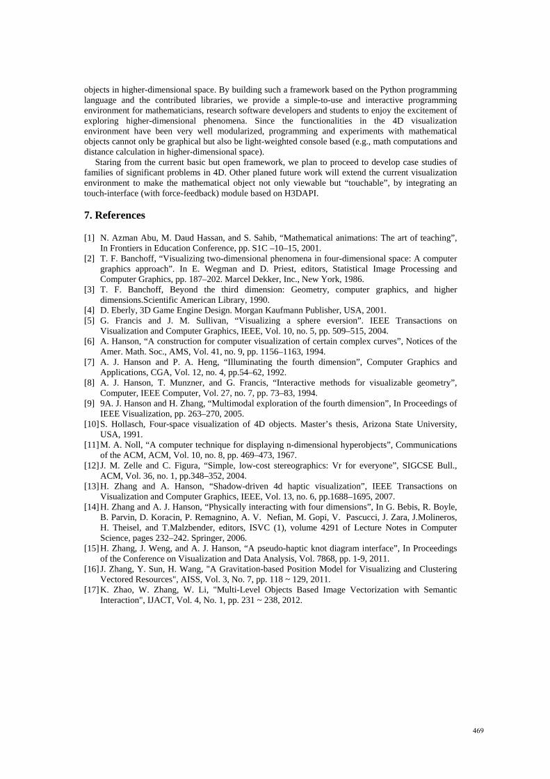
This can be trivially extended to an interesting 4D analogy in Figure 8. A point inside a 2-sphere can’t seem to escape when embedded in 3D initially, we all know this is true since in our everyday life we use containers to hold various stuffs (a sealed container is topologically equivalent to a 2-sphere). Just like a point can escape from a ring in 3D, a point can escape from a 2-sphere in 4D. If we apply a general 4D rotation, each vertex will acquire a non-vanishing 4D “eye coordinate” or depth w; if we again apply 2D forces to the point (e.g., along w direction), we see that we are able to “pull” the point from the 2-sphere in 4D just like we pull the point from a ring in 3D (see Figure 13 (c)). The apparent intersections between the point and the 2-sphere are just an illusion in 4D, and a 2-sphere simply can’t trap a point any more in 4D (see Figure 9 (d)).


467

(a) (b) (c)

(d) (e) (f)

Figure 7. (a)- (b) Flattened 4D cloth behaves like 3D cloth. (c) With a general 4D rotation applied, the 4D cloth appears to be self-intersecting in the 3D projection while in fact having no actual intersections of any kind in the four-dimensional space. (d)- (f) Projected images from 4D to subspaces YZW, XZW, and XYW. The projected images reveal that the cloth-like surface is still smooth and continuous in the

fourth dimension, even if it appears to be self-intersecting in (c).

(a) (b) (c) (d)

Figure 8. (a)- (b) A point is trapped inside a ring when embedded in 2D. (c) With a general 3D rotation applied, a 2D force can be applied to the point then to pull the point outside of the ring, which are now embedded in 3D.

(a) (b) (c) (d)

Figure 9. (a)- (b) A point trapped inside a 2-sphere when embedded in 3D. (c)- (d) With a general 4D rotation applied, the point can escape from the 2-sphere embedded in 4D. 6. Conclusion and future work

We have demonstrated a Python-based 4D visualization environment for prototyping and experimenting with mathematical and physical phenomena in 2D, 3D and 4D. Families of computational modules have been developed for generating interactive experience with mathematical

468

objects in higher-dimensional space. By building such a framework based on the Python programming language and the contributed libraries, we provide a simple-to-use and interactive programming environment for mathematicians, research software developers and students to enjoy the excitement of exploring higher-dimensional phenomena. Since the functionalities in the 4D visualization environment have been very well modularized, programming and experiments with mathematical objects cannot only be graphical but also be light-weighted console based (e.g., math computations and distance calculation in higher-dimensional space).

Staring from the current basic but open framework, we plan to proceed to develop case studies of families of significant problems in 4D. Other planed future work will extend the current visualization environment to make the mathematical object not only viewable but “touchable”, by integrating an touch-interface (with force-feedback) module based on H3DAPI.

7. References [1] N. Azman Abu, M. Daud Hassan, and S. Sahib, “Mathematical animations: The art of teaching”,

In Frontiers in Education Conference, pp. S1C –10–15, 2001. [2] T. F. Banchoff, “Visualizing two-dimensional phenomena in four-dimensional space: A computer

graphics approach”. In E. Wegman and D. Priest, editors, Statistical Image Processing and Computer Graphics, pp. 187–202. Marcel Dekker, Inc., New York, 1986.

[3] T. F. Banchoff, Beyond the third dimension: Geometry, computer graphics, and higher dimensions.Scientific American Library, 1990.

[4] D. Eberly, 3D Game Engine Design. Morgan Kaufmann Publisher, USA, 2001. [5] G. Francis and J. M. Sullivan, “Visualizing a sphere eversion”. IEEE Transactions on

Visualization and Computer Graphics, IEEE, Vol. 10, no. 5, pp. 509–515, 2004. [6] A. Hanson, “A construction for computer visualization of certain complex curves”, Notices of the

Amer. Math. Soc., AMS, Vol. 41, no. 9, pp. 1156–1163, 1994. [7] A. J. Hanson and P. A. Heng, “Illuminating the fourth dimension”, Computer Graphics and

Applications, CGA, Vol. 12, no. 4, pp.54–62, 1992. [8] A. J. Hanson, T. Munzner, and G. Francis, “Interactive methods for visualizable geometry”,

Computer, IEEE Computer, Vol. 27, no. 7, pp. 73–83, 1994. [9] 9A. J. Hanson and H. Zhang, “Multimodal exploration of the fourth dimension”, In Proceedings of

IEEE Visualization, pp. 263–270, 2005. [10] S. Hollasch, Four-space visualization of 4D objects. Master’s thesis, Arizona State University,

USA, 1991. [11] M. A. Noll, “A computer technique for displaying n-dimensional hyperobjects”, Communications

of the ACM, ACM, Vol. 10, no. 8, pp. 469–473, 1967. [12] J. M. Zelle and C. Figura, “Simple, low-cost stereographics: Vr for everyone”, SIGCSE Bull.,

ACM, Vol. 36, no. 1, pp.348–352, 2004. [13] H. Zhang and A. Hanson, “Shadow-driven 4d haptic visualization”, IEEE Transactions on

Visualization and Computer Graphics, IEEE, Vol. 13, no. 6, pp.1688–1695, 2007. [14] H. Zhang and A. J. Hanson, “Physically interacting with four dimensions”, In G. Bebis, R. Boyle,

B. Parvin, D. Koracin, P. Remagnino, A. V. Nefian, M. Gopi, V. Pascucci, J. Zara, J.Molineros, H. Theisel, and T.Malzbender, editors, ISVC (1), volume 4291 of Lecture Notes in Computer Science, pages 232–242. Springer, 2006.

[15] H. Zhang, J. Weng, and A. J. Hanson, “A pseudo-haptic knot diagram interface”, In Proceedings of the Conference on Visualization and Data Analysis, Vol. 7868, pp. 1-9, 2011.

[16] J. Zhang, Y. Sun, H. Wang, "A Gravitation-based Position Model for Visualizing and Clustering Vectored Resources", AISS, Vol. 3, No. 7, pp. 118 ~ 129, 2011.

[17] K. Zhao, W. Zhang, W. Li, "Multi-Level Objects Based Image Vectorization with Semantic Interaction", IJACT, Vol. 4, No. 1, pp. 231 ~ 238, 2012.

469

python based 4d visualization environment · python based 4d visualization environment 1lin jing,...

Documents