python stat
TRANSCRIPT

Statistics for Python
An extension module for the Python scripting language
Michiel de Hoon, Columbia University

29 August 2008Statistics for Python, an extension module for the Python scripting language.
Copyright c© 2006 Michiel Jan Laurens de HoonThis library was written at the Center for Computational Biology and Bioinformatics,Columbia University, 1130 Saint Nicholas Avenue, New York, NY 10032, United States.Contact: mjldehoonx_AT_yahoo.com
Permission to use, copy, modify, and distribute this software and its documentation with orwithout modifications and for any purpose and without fee is hereby granted, provided thatany copyright notices appear in all copies and that both those copyright notices and thispermission notice appear in supporting documentation, and that the names of the contrib-utors or copyright holders not be used in advertising or publicity pertaining to distributionof the software without specific prior permission.
THE CONTRIBUTORS AND COPYRIGHT HOLDERS OF THIS SOFTWARE DIS-CLAIM ALL WARRANTIES WITH REGARD TO THIS SOFTWARE, INCLUDING ALLIMPLIED WARRANTIES OF MERCHANTABILITY AND FITNESS, IN NO EVENTSHALL THE CONTRIBUTORS OR COPYRIGHT HOLDERS BE LIABLE FOR ANYSPECIAL, INDIRECT OR CONSEQUENTIAL DAMAGES OR ANY DAMAGES WHAT-SOEVER RESULTING FROM LOSS OF USE, DATA OR PROFITS, WHETHER IN ANACTION OF CONTRACT, NEGLIGENCE OR OTHER TORTIOUS ACTION, ARIS-ING OUT OF OR IN CONNECTION WITH THE USE OR PERFORMANCE OF THISSOFTWARE.

i
Table of Contents

Chapter 1: Introduction 1
1 Introduction
Statistics for Python is an extension module, written in ANSI-C, for the Python scriptinglanguage. Currently, this extension module contains some routines to estimate the proba-bility density function from a set of random variables.Statistics for Python was released under the Python License.
Michiel de Hoon (mdehoon_AT_c2b2.columbia.edu; mdehoon_AT_cal.berkeley.edu)Center for Computational Biology and Bioinformatics, Columbia University.

Chapter 2: Descriptive statistics 2
2 Descriptive statistics
Statistics for Python currently contains four functions for descriptive statistics: The mean,the median, the Pearson correlation, and a function to fit a linear regression line.
2.1 Univariate descriptive statistics
B. P. Welford: “Note on a method for calculating corrected sums of squares and products.”Technometrics 4(3): 419-420 (1962).Peter M. Neely: “Comparison of several algorithms for computation of means, standarddeviations and correlation coefficients.” Communications of the ACM 9(7): 496-499 (1966).
The arithmetic mean is defined as
x =1
n
n∑
i=1
xi
The statistical median of the data xi is defined as
x =
{
x′(n+1)/2, if n is odd;
12
(
x′n/2 + x′
1+n/2
)
, if n is even.
where we find the array x′ by sorting the array x.
The variance in a random variable x is defined as
σ2x = E
[
(x − µx)2]
Given n data of x, the unbiased estimate of the variance is
σ2x =
1
n − 1
n∑
i=1
x2i −
1
n
(
n∑
i=1
xi
)2
.
For the maximum-likelihood estimate of the variance, which is a biased estimate, we divideby n instead of n − 1.
The variance in this library is implemented using the algorithm proposed by Welford(1962), which avoids the round-off errors associated with a direct calculation of the variance.
2.2 Multivariate descriptive statistics
Ronald A. Fisher: “Statistical Methods for Research Workers”, chapter VII. Oliver andBoyd, Edinburgh/London (1925).”

Chapter 2: Descriptive statistics 3
2.2.1 Covariance
The covariance between two random variables x and y is defined as
σxy = E((x − µx) (y − µy))
Given n paired data of x and y, the unbiased estimate of their covariance is
σxy =1
n − 1
[
n∑
i=1
xiyi −1
n
(
n∑
i=1
xi
)(
n∑
i=1
yi
)]
;
for the maximum-likelihood estimate of the covariance, which is a biased estimate, we divideby n instead of n − 1.
The covariance is calculated using the algorithm proposed by Welford (1962) to avoidround-off errors.
2.2.2 Correlation
Statistics for Python includes the following correlation measures:
• Pearson correlation
• Spearman rank correlation
• Intraclass correlation
The Pearson correlation is calculated using the algorithm proposed by Welford (1962)to avoid round-off errors.
The intraclass correlation follows the definition by Fisher:
r1,2 =
∑ni=1 (xi,1 − x1,2) (xi,2 − x1,2)
12
∑ni=1 (xi,1 − x1,2)
2+ 1
2
∑ni=1 (xi,2 − x1,2)
2
in which
x1,2 =1
2
n∑
i=1
(xi,1 + xi,2)
To avoid round-off error, the intraclass correlation is calculated using a recursion formulasimilar to the Welford algorithm:
r1,2 =N
(n)1,2
D(n)1 + D
(n)2 + n
4
(
x(n)1 − x
(n)2
)2
in which N(n)1,2 , D
(n)1 , D
(n)2 , x
(n)1 , and x
(n)2 are calculated from the recursion formulae
x(j)1 =
j − 1
jx
(j−1)1 +
1
jxj,1
x(j)2 =
j − 1
jx
(j−1)2 +
1
jxj,2
N(j)1,2 = N
(j−1)1,2 +
j − 1
4j
(
x(j−1)1 + x
(j−1)2 − xj,1 − xj,2
)2
− 1
4(xj,1 − xj,2)
2
D(j)1 = D
(j−1)1 +
j − 1
2j
(
x(j−1)1 − xj,1
)2
D(j)2 = D
(j−1)2 +
j − 1
2j
(
x(j−1)2 − xj,2
)2
with N(0)1,2 = D
(0)1 = D
(0)2 = x
(0)1 = x
(0)2 = 0.

Chapter 2: Descriptive statistics 4
2.2.3 Linear regression
Calculate the intercept and slope of a linear regression line through a cloud of points.
2.3 Usage
2.3.1 Mean
The function mean returns the arithmetic mean of an array of data.>>> mean(x)
Arguments
• x
A one-dimensional array containing the data for which to calculate the mean.
Return values
• The arithmetic mean of the data x.
2.3.2 Median
The function median returns the median of an array of data.>>> median(x)
Arguments
• x
A one-dimensional array containing the data for which to calculate the median.
Return values
• The median of the data x.
2.3.3 Variance
The function variance calculates the variance of a one-dimensional array of data.>>> variance(x, mode = "Unbiased")
Arguments
• x
A one-dimensional array containing the data for which to calculate the variance;
• mode
For mode equal to Unbiased (which is the default value), the function variance returnsthe unbiased estimate of the variance. For mode equal to ML, the function returns themaximum-likelihood estimate of the variance, which is a biased estimate.
Return values
• The variance in x.
Chapter 2: Descriptive statistics 5
2.3.4 Covariance
The function covariance calculates the covariance matrix of an array of data.>>> covariance(x, y = None, mode = "Unbiased")
Arguments
• x
Either a one-dimensional array or a two-dimensional array containing the data forwhich to calculate the covariance.
• If x is a one-dimensional array and y==None, then this function returns the varianceof x;
• If both x and y are one-dimensional arrays with the same length, covariance
returns the covariance between x and y;
• If x is a two-dimensional array, then covariance returns the covariance matrix ofx; y is ignored.
• y
A one-dimensional array of the same length as x, or None;
• mode For mode equal to Unbiased (which is the default value), the function covariance
returns the unbiased estimate of the covariance. For mode equal to ML, the functionreturns the maximum-likelihood estimate of the covariance, which is a biased estimate.
Return values
• If x is one-dimensional and y==None: the variance in x;
• If x and y are both one-dimensional and have the same length: the covariance betweenx and y;
• If x is two-dimensional: the covariance matrix between the columns of x. Element[i,j] of the covariance matrix contains the covariance between columns x[:,i] andx[:,j].
2.3.5 Correlation
The function correlation calculates the correlation matrix of an array of data.>>> correlation(x, y = None, method = "Pearson")
Arguments
• x
Either a one-dimensional array or a two-dimensional array containing the data forwhich to calculate the correlation.
• If x is a one-dimensional array and y==None, then this function returns 1.0;
• If both x and y are one-dimensional arrays with the same length, correlationreturns the correlation between x and y;
• If x is a two-dimensional array, then correlation returns the correlation matrixof x; y is ignored.

Chapter 2: Descriptive statistics 6
• y
A one-dimensional array of the same length as x, or None;
• method Determines which type of correlation is calculated:
• "Pearson": The Pearson correlation (default);
• "Spearman": The Spearman rank correlation;
• "Intraclass": The intraclass correlation.
Return values
• If x is one-dimensional and y==None: 1.0;
• If x and y are both one-dimensional and have the same length: the correlation betweenx and y;
• If x is two-dimensional: the correlation matrix between the columns of x. Element[i,j] of the correlation matrix contains the correlation between columns x[:,i] andx[:,j].
2.3.6 Linear regression
The function regression returns the intercept and slope of a linear regression line fit totwo arrays x and y.>>> a, b = regression(x,y)
Arguments
• x
A one-dimensional array of data;
• y
A one-dimensional array of data.
The size of x and y should be equal.
Return values
• a
The intercept of the linear regression line;
• b
The slope of the linear regression line.

Chapter 3: Kernel estimation of probability density functions 7
3 Kernel estimation of probability densityfunctions
B. W. Silverman: “Density Estimation for Statistics and Data Analysis”, Chapter 3. Chap-man and Hall, New York, 1986.D. W. Scott: “Multivariate Density Estimation; Theory, Practice, and Visualization”,Chapter 6. John Wiley and Sons, New York, 1992.
Suppose we have a set of observations xi, and we want to find the probability densityfunction of the distribution from which these data were drawn. In parametric density esti-mations, we choose some distribution (such as the normal distribution or the extreme valuedistribution) and estimate the values of the parameters appearing in these functions fromthe observed data. However, often the functional form of the true density function is notknown. In this case, the probability density function can be estimated non-parametricallyby using a kernel density estimation.
3.1 Kernel estimation of the density function
Histograms are commonly used to represent a statistical distribution. To calculate a his-togram, we divide the data into bins of size 2h, and count the number of data in each bin.Formally, we can write this as
f (x) =1
nh
n∑
i=1
k
(
x − xi
h
)
,
where the function k is defined by
k (t) =
{ 12, |t| ≤ 1;
0, |t| > 1,
and h is called the bandwidth, smoothing parameter, or window width. Here, the probabilitydensity is estimated for a given value of x which corresponds to the center of each bin in thehistogram. More generally, by varying x we can estimate the probability density functionf (x) as a function of x.
Using the kernel function k as defined above yields the naıve estimator of the probabilitydensity function. As the kernel function is not continuous, the naıve estimator tends toproduce jagged probability density functions. Hence, we replace the flat-top kernel functionby some smooth (and usually symmetric and non-negative) function. In order to guaranteethat the estimated density function integrates to unity, we also require
∫ ∞
−∞k (t) dt = 1.
Some commonly used kernel functions are listed in the table below. The Epanechnikovkernel is used by default, as it can (theoretically) minimize the mean integrated square errorof the estimation. In practice, there is little difference in the integrated square error betweenprobability density functions estimated with different kernels, and it may be worthwhile tochoose a different kernel based on other considerations, such as differentiability.

Chapter 3: Kernel estimation of probability density functions 8
Mnemonic Kernel name Function Optimalbandwidth h
’u’ Uniform k (t) =
{ 12, |t| ≤ 1;
0, |t| > 1.σ(
12√
πn
)1
5
’t’ Triangle k (t) =
{
1 − |t| , |t| ≤ 1;0, |t| > 1.
σ(
64√
πn
)1
5
’e’ Epanechnikov k (t) =
{ 34(1 − t2) , |t| ≤ 1;
0, |t| > 1.σ(
40√
π
n
)1
5
’b’ Biweight/quartic k (t) =
{
1516
(1 − t2)2, |t| ≤ 1;
0, |t| > 1.σ(
280√
π3n
)1
5
’3’ Triweight k (t) =
{
3532
(1 − t2)3, |t| ≤ 1;
0, |t| > 1.σ(
25200√
π143n
)1
5
’c’ Cosine k (t) =
{ π4
cos(
π2t)
, |t| ≤ 1;0, |t| > 1.
σ(
π13/2
6n(π2−8)2
)1
5
’g’ Gaussian k (t) = 1√2π
exp(
− 12t2)
σ(
43n
)1
5
Estimating the probability density function with the Gaussian kernel is more computation-ally intensive than with other kernels, as it has infinite support (i.e., k (t) is nonzero for allt).
3.2 Kernel estimation of the cumulative probability density
By integrating the estimated probability density function, we obtain an estimate for thecumulative density function F (x):
F (x) =
∫ x
−∞f (t) dt =
1
n
n∑
i=1
K
(
x − xi
h
)
,
where K is defined as the primitive of the kernel function k:
K (x) ≡∫ x
−∞k (t) dt.
This software package contains a Python function to calculate this estimate directly froma set of data, as well as a function to estimate the complementary cumulative probabilitydensity, defined as
F ′ (x) ≡ 1 − F (x) .
The complementary cumulative probability density F ′ (x) can be interpreted as the tailprobability p of the random variable to be equal to or larger than x assuming that it isdrawn from the distribution described by f .
3.3 Choosing the bandwidth
The bandwidth h determines how smooth the estimated probability density function willbe: A larger value for h leads to a smoother probability density function, as it is averagedover more data points. Often, a suitable bandwith can be chosen subjectively based on theapplication at hand. Alternatively, we may choose the bandwidth such that it minimizes the

Chapter 3: Kernel estimation of probability density functions 9
asymptotic mean integrated square error. This optimal bandwidth depends on the numberof observations n, the standard deviation σ of the observed data, and the kernel function.The formulas for the optimal bandwidth are given in the table above. To make things easy,this software package contains a Python function to calculate the optimal bandwidth fromthe data.
3.4 Usage
3.4.1 Estimating the probability density function
The function pdf estimates the probability density function from the observed data. Youcan either specify the values of x at which you want to estimate the value y of the probabilitydensity function explicitly:>>> y = pdf(data, x, weight = None, h = None, kernel = ’Epanechnikov’)
or you can let the function choose x for you:>>> y, x = pdf(data, weight = None, h = None, kernel = ’Epanechnikov’, n = 100)
In the latter case, the returned array x contains n equidistant data points covering thedomain where f (x) is nonzero.
Arguments
• data
The one-dimensional array data contains the observed data from which the probabilitydensity function is estimated;
• weight
The one-dimensional array weight, if given, contains the weights for the observed data.If weight==None, then each data point receives an equal weight 1.
• x
The value(s) at which the probability density function will be estimated (either a singlevalue, or a 1D array of values). If you don’t specify x, the function pdf will create x
as a 1D array of n values for you and return it together with the estimated probabilitydensity function;
• h
The bandwidth to be used for the estimation. If h is not specified (and also if the userspecifies a zero or negative h), the optimal bandwidth is used (which can be calculatedexplicitly by the function bandwidth);
• kernel
The kernel function can be specified by its name (case is ignored), or by a one-charactermnemonic:
’E’ or ’Epanechnikov’Epanechnikov kernel (default)
’U’ or ’Uniform’Uniform kernel
’T’ or ’Triangle’Triangle kernel

Chapter 3: Kernel estimation of probability density functions 10
’G’ or ’Gaussian’
Gaussian kernel
’B’ or ’Biweight’Quartic/biweight kernel
’3’ or ’Triweight’Triweight kernel
’C’ or ’Cosine’Cosine kernel
• n
The number of points for which the probability density function is to be estimated.This argument is meaningful only if you don’t specify x explicitly; passing both x andn raises an error. Default value of n is 100.
Return values
• If you specified x explicitly: The estimated probability density, estimated at at thevalues in x;
• If you did not specify x explicitly: The estimated probability density, as well as thecorresponding values of x.
3.4.2 Estimating the cumulative probability density function
The function cpdf estimates the cumulative probability density function from the observeddata. You can either specify the values of x at which you want to estimate the value y ofthe cumulative probability density function explicitly:>>> y = cpdf(data, x, h = None, kernel = ’Epanechnikov’)
or you can let the function choose x for you:>>> y, x = cpdf(data, h = None, kernel = ’Epanechnikov’, n = 100)
In the latter case, the returned array x contains n equidistant data points covering thedomain where f (x) is nonzero; the estimated cumulative probability density is constant(either 0 or 1) outside of this domain.
Arguments
• data
The one-dimensional array data contains the observed data from which the cumulativeprobability density function is estimated;
• x
The value(s) at which the cumulative probability density function will be estimated(either a single value, or a 1D array of values). If you don’t specify x, the functioncpdf will create x as a 1D array of n values for you and return it together with theestimated cumulative probability density function.
• h
The bandwidth to be used for the estimation. If h is not specified (and also if the userspecifies a zero or negative h), the optimal bandwidth is used (which can be calculatedexplicitly by the function bandwidth).

Chapter 3: Kernel estimation of probability density functions 11
• kernel
The kernel function can be specified by its name (case is ignored), or by a one-charactermnemonic:
’E’ or ’Epanechnikov’Epanechnikov kernel (default)
’U’ or ’Uniform’Uniform kernel
’T’ or ’Triangle’Triangle kernel
’G’ or ’Gaussian’
Gaussian kernel
’B’ or ’Biweight’Quartic/biweight kernel
’3’ or ’Triweight’Triweight kernel
’C’ or ’Cosine’Cosine kernel
• n
The number of points for which the cumulative probability density function is to beestimated. This argument is meaningful only if you don’t specify x explicitly; passingboth x and n raises an error. Default value of n is 100.
Return values
• If you specified x explicitly: The estimated cumulative probability density, estimatedat at the values in x;
• If you did not specify x explicitly: The estimated cumulative probability density, aswell as the corresponding values of x.
3.4.3 Estimating the complement of the cumulative probability
density function
The function cpdfc estimates the complement of the cumulative probability density functionfrom the observed data. You can either specify the values of x at which you want to estimatethe value y of the complement of the cumulative probability density function explicitly:>>> y = cpdfc(data, x, h = None, kernel = ’Epanechnikov’)
or you can let the function choose x for you:>>> y, x = cpdfc(data, h = None, kernel = ’Epanechnikov’, n = 100)
In the latter case, the returned array x contains n equidistant data points covering thedomain where f (x) is nonzero; the estimated complement of the cumulative probabilitydensity is constant (either 0 or 1) outside of this domain.
Arguments
• data
The one-dimensional array data contains the observed data from which the complementof the cumulative probability density function is estimated.
Chapter 3: Kernel estimation of probability density functions 12
• x
The value(s) at which the complement of the cumulative probability density functionwill be estimated (either a single value, or a 1D array of values). If you don’t specify x,the function cpdfc will create x as a 1D array of n values for you and return it togetherwith the estimated complement of the cumulative probability density function.
• h
The bandwidth to be used for the estimation. If h is not specified (and also if the userspecifies a zero or negative h), the optimal bandwidth is used (which can be calculatedexplicitly by the function bandwidth).
• kernel
The kernel function can be specified by its name (case is ignored), or by a one-charactermnemonic:
’E’ or ’Epanechnikov’Epanechnikov kernel (default)
’U’ or ’Uniform’Uniform kernel
’T’ or ’Triangle’Triangle kernel
’G’ or ’Gaussian’
Gaussian kernel
’B’ or ’Biweight’Quartic/biweight kernel
’3’ or ’Triweight’Triweight kernel
’C’ or ’Cosine’Cosine kernel
• n
The number of points for which the complement of the cumulative probability densityfunction is to be estimated. This argument is meaningful only if you don’t specify x
explicitly; passing both x and n raises an error. Default value of n is 100.
Return values
• If you specified x explicitly: The estimated cumulative probability density, estimatedat at the values in x;
• If you did not specify x explicitly: The estimated cumulative probability density, aswell as the corresponding values of x.
3.4.4 Calculating the optimal bandwidth
The function bandwidth calculates the optimal bandwidth from the observed data for agiven kernel:>>> h = bandwidth(data, kernel=’Epanechnikov’)

Chapter 3: Kernel estimation of probability density functions 13
Arguments
• data
A one-dimensional array data contains the observed data from which the probabilitydensity function will be calculated;
• kernel
The kernel function can be specified by its name (case is ignored), or by a one-charactermnemonic:
’E’ or ’Epanechnikov’Epanechnikov kernel (default)
’U’ or ’Uniform’Uniform kernel
’T’ or ’Triangle’Triangle kernel
’G’ or ’Gaussian’
Gaussian kernel
’B’ or ’Biweight’Quartic/biweight kernel
’3’ or ’Triweight’Triweight kernel
’C’ or ’Cosine’Cosine kernel
Return value
The function bandwidth returns the optimal bandwidth for the given data, using the spec-ified kernel. This bandwidth can subsequently be used when estimating the (cumulative)probability density with pdf, cpdf, or cpdfc.

Chapter 3: Kernel estimation of probability density functions 14
3.5 Examples
3.5.1 Estimating a probability density function
We use Numerical Python’s random module to draw 100 random numbers from a standardnormal distribution.
>>> from numpy.random import standard_normal
>>> data = standard_normal(100)
We estimate the probability density function, using the default Epanechnikov kernel andthe default value for the bandwidth:>>> import statistics
>>> y, x = statistics.pdf(data)
The estimated probability function y as a function of x is drawn below (figure created byPygist).
Chapter 3: Kernel estimation of probability density functions 15
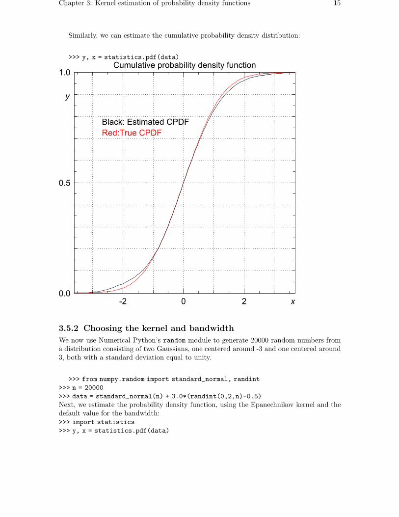
Similarly, we can estimate the cumulative probability density distribution:
>>> y, x = statistics.pdf(data)
3.5.2 Choosing the kernel and bandwidth
We now use Numerical Python’s random module to generate 20000 random numbers froma distribution consisting of two Gaussians, one centered around -3 and one centered around3, both with a standard deviation equal to unity.
>>> from numpy.random import standard_normal, randint
>>> n = 20000
>>> data = standard_normal(n) + 3.0*(randint(0,2,n)-0.5)
Next, we estimate the probability density function, using the Epanechnikov kernel and thedefault value for the bandwidth:>>> import statistics
>>> y, x = statistics.pdf(data)

Chapter 3: Kernel estimation of probability density functions 16

Chapter 3: Kernel estimation of probability density functions 17
The choice of kernel function usually has a minor effect on the estimated probabilitydensity function:>>> y, x = statistics.pdf(data, kernel="Gaussian")

Chapter 3: Kernel estimation of probability density functions 18
Now, let’s find out the default value for the bandwidth was:>>> statistics.bandwidth(data)
0.58133427540755089
Choosing a bandwidth much smaller than the default value results in overfitting:>>> y, x = statistics.pdf(data, h = 0.58133427540755089/10)

Chapter 3: Kernel estimation of probability density functions 19
Choosing a bandwidth much larger than the default value results in oversmoothing:>>> y, x = statistics.pdf(data, h = 0.58133427540755089*4)

Chapter 3: Kernel estimation of probability density functions 20
3.5.3 Approaching the extreme value distribution
Suppose we generate m random numbers u from a standard normal distribution, and definex the maximum of these m numbers. By repeating this n times, we obtain n randomnumbers whose distribution, for m large, approaches the extreme value distribution.
Given that the random numbers u are drawn from a standard normal distribution, wecan calculate the distribution of x analytically:
fm (x) =m√2π
(
1
2− 1
2erf
(
x√2
))m−1
exp
(
−1
2x2
)
. However, in general the distribution of u, and therefore x is unknown, except that for m
large we can approximate the distribution of x by an extreme value distribution:
fa,b (x) =1
bexp
(
a − x
b− exp
(
a − x
b
))
,
where a and b are estimated from the mean and variance of x:
µ = a + bγ;
σ2 =1
6π2b2,
where γ ≈ 0.577216 is the Euler-Mascheroni constant.
Here, we generate n = 1000 random numbers x, for increasing values of m, and approx-imate the distribution of x by a normal distribution, an extreme value distribution, and bythe kernel-based estimate.
>>> import statistics
>>> from numpy.random import standard_normal
>>> n = 1000
>>> m = 1
>>> data = array([max(standard_normal(m)) for i in range(n)])
>>> y, x = statistics.pdf(data)
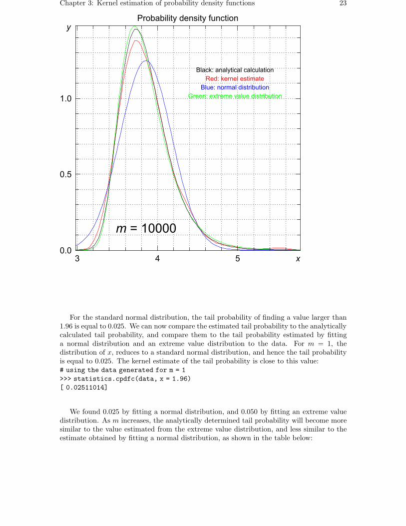
The estimated probability density, together with the analytically determined probabilitydensity, a normal distribution, and the extreme value distribution are drawn in the figuresbelow for increasing values of m.
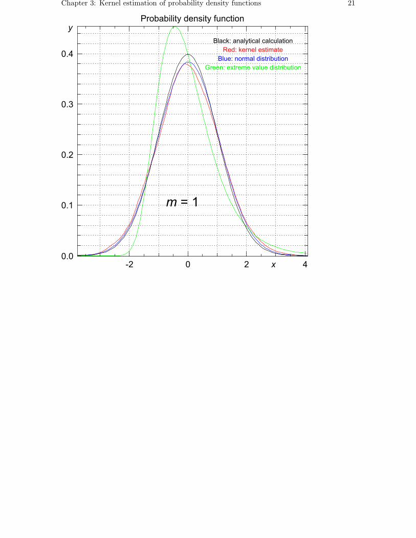
Chapter 3: Kernel estimation of probability density functions 21

Chapter 3: Kernel estimation of probability density functions 22
Chapter 3: Kernel estimation of probability density functions 23
For the standard normal distribution, the tail probability of finding a value larger than1.96 is equal to 0.025. We can now compare the estimated tail probability to the analyticallycalculated tail probability, and compare them to the tail probability estimated by fittinga normal distribution and an extreme value distribution to the data. For m = 1, thedistribution of x, reduces to a standard normal distribution, and hence the tail probabilityis equal to 0.025. The kernel estimate of the tail probability is close to this value:# using the data generated for m = 1
>>> statistics.cpdfc(data, x = 1.96)
[ 0.02511014]
We found 0.025 by fitting a normal distribution, and 0.050 by fitting an extreme valuedistribution. As m increases, the analytically determined tail probability will become moresimilar to the value estimated from the extreme value distribution, and less similar to theestimate obtained by fitting a normal distribution, as shown in the table below:

Chapter 3: Kernel estimation of probability density functions 24
m Exact(analytic)
Kernelestimate
Normaldistribution
Extreme valuedistribution
1 0.0250 0.0251 0.0250 0.04973 0.0310 0.0310 0.0250 0.04655 0.0329 0.0332 0.0250 0.041110 0.0352 0.0355 0.0250 0.045125 0.0374 0.0377 0.0250 0.0409100 0.0398 0.0396 0.0250 0.0514200 0.0405 0.0407 0.0250 0.04821000 0.0415 0.0417 0.0250 0.045410000 0.0424 0.0427 0.0250 0.0506

Chapter 4: Installation instructions 25
4 Installation instructions
In the instructions below, <version> refers to the version number. This software complieswith the ANSI-C standard; compilation should therefore be straightforward.
First, make sure that Numerical Python (version 1.1.1 or later) is installed on yoursystem. To check your Numerical Python version, type>>> import numpy; print numpy.version.version
at the Python prompt.
To install Statistics for Python, unpack the file:gunzip statistics-<version>.tar.gz
tar -xvf statistics-<version>.tar
and change to the directory statistics-<version>. From this directory, typepython setup.py config
python setup.py build
python setup.py install
This will configure, compile, and install the library. If the installation was successful, you canremove the directory statistics-<version>. For Python on Windows, a binary installeris available from http://bonsai.ims.u-tokyo.ac.jp/~mdehoon/software/python.