q-value based particle swarm optimization for ... · q-value based particle swarm optimization for...

Q-Value Based Particle Swarm Optimization for Reinforcement Neuro-

Fuzzy System Design

Yi-Chang Cheng Dept. of Electrical Engineering National Chiao Tung University

HsinChu, Taiwan [email protected]

Sheng-Fuu Lin Dept. of Electrical Engineering National Chiao Tung University


Chi-Yao Hsu Dept. of Electrical Engineering National Chiao Tung University


Abstract—This paper proposes a combination of particle swarm optimization (PSO) and Q-value based

safe reinforcement learning scheme for neuro-fuzzy systems (NFS). The proposed Q-value based particle swarm

optimization (QPSO) fulfills PSO-based NFS with reinforcement learning; that is, it provides PSO-based NFS

an alternative to learn optimal control policies under environments where only weak reinforcement signals are

available. The reinforcement learning scheme is designed by Lyapunov principles and enjoys a number of

practical benefits, including the ability of maintaining a system's state in a desired operating range and efficient

learning. In the QPSO, parameters on a NFS are encoded in a particle evaluated by Q-value. The Q-value

cumulates the reward received during a learning trial and is used as the fitness function for PSO evolution.

During the trail, one particle is selected from the swarm; meanwhile, a corresponding NFS is built and applied

to the environment with an immediate feedback reward. The applicability of QPSO is shown through

simulations in single-link and double-link inverted pendulum system.

Keywords- Neuro-fuzzy system, particle swarm optimization, reinforcement learning, Q-learning.

I. INTRODUCTION In recent years, the application of neuro-fuzzy systems in control engineering has become a popular research

topic [1]-[3]. In general, the way of tuning the parameters on a NFS can be divided into two categories: supervised learning [4] and reinforcement learning [5].

First, supervised learning is a machine learning technique for updating its parameters from training data. The training data is composed of pairs of inputs, and desired outputs. The object of the supervised learning is to predict the output value of the NFS for any valid input data after its parameters have been trained by a number of training data. However, for many control tasks, training data are usually difficult or too costly, or even not accessible. As a result, reinforcement learning is more practicable than supervised learning in many occasions.

Yi-Chang Cheng et al. / International Journal on Computer Science and Engineering (IJCSE)

ISSN : 0975-3397 Vol. 3 No. 10 October 2011 3477

In reinforcement learning, the agent receives from its environment a reinforcement signal at each time step. This signal could be either a reward or a punishment. Meanwhile, the agent explores actions from the action set, and finds out which action yields the greatest reward. To solve reinforcement problem, temporal difference (TD) [6]-[8] is one of the most common method. In TD learning, learners don’t have to wait until the end of a trial; instead, TD methods need wait only one time step. This is crucial for applications that have very long trials or tasks that are continuous and have no trials at all. Q-learning [9] is a powerful and easy-implementing TD-based approach. It is a reinforcement learning technique that works by updating a simple action-value iteration function. This function gives the measurement of taking a given action in a given state.

Besides TD methods, many evolutionary algorithms such as PSO [10]-[12], genetic algorithm (GA) [13], evolutionary programming [14], and evolution strategies [15], are popular for solving reinforcement learning tasks. These learning procedures are based on populations made of individuals with specific behaviors similar to certain biological phenomena. Individuals keep exploring the solution space and exploiting information between individuals while evolution proceeding. In general, by means of exploring and exploiting, evolutionary algorithms are less likely to be trapped at the local optimum. Many researches on using evolutionary algorithm for solving reinforcement learning tasks have been proposed recently [16]-[17]. In [16], authors propose a swarm intelligence based reinforcement learning (SWIRL) method to train artificial neural networks (ANN). Authors apply ant colony optimization to select ANN topology and apply the PSO to adjust ANN connection weights. In [17], Lin and Hsu present a reinforcement hybrid learning algorithm (R-HELA) combining the compact GA (CGA) [18] and the modified variable-length GA (VGA) [19] on recurrent wavelet-based NFS. A counter is used to accumulate the time steps until the control task fails and the accumulated values are fed into individuals as fitness functions. Lin and Hsu’s model is very effective; however, its fitness function only indicates how long can the controller work well instead of measuring how soon the system can meet the control goal, which is also very important in reinforcement learning. There is also a growing interest in combining the advantages of evolutionary algorithms and TD-based reinforcement learning [20]-[21]. In [20], a TD and GA based reinforcement learning (TDGAR) is proposed. Authors propose a neural structure composed of two feedforward networks for reinforcement learning, the critic network and the action network. The critic network predicts the external signal provides a more informative internal signal to the action network. The action network uses GA to determine the output of the learning system. The weight update rule for the hidden layer of the critic network is based on error backpropagation. In [21], an on-line clustering and Q-value based GA reinforcement learning for fuzzy system (CQGAF) is proposed. In one generation CQGAF learning, one individual is applied to the environment to estimate the fitness function, Q-value, and Q-values of other individuals are updated by eligibility trace. The GA operation is performed by the end of each trial and creates a new generation of individuals. In [22], authors proposed a recurrent wavelet-based NFS with a reinforcement group cooperation-based symbiotic evolution (R-GCSE) algorithm. In [22], a population is divided to several groups. The R-GCSE has a good ability of parameter learning by adopting the concept that each group formed by a set of chromosomes cooperates with other groups to generate better chromosomes.

Although the aforementioned reinforcement learning methods work well in many applications, there is an issue remains to be solved. No fitness function in these methods indicates how soon the learning agents can control the system's state into a set of goal states. Sure there is no need to define the fitness function that way if there is no guidance provided to the controller of how to maintain the system's state in a desired operating range. As a result, in the proposed QPSO, we use the concept of Lyapunov design [23] for constructing safe reinforcement learning agents. We also manipulate our fitness function so that it can indicate how soon the controller achieves its control goal. In our method, a TSK-type NFS [24] is incorporated in the learning system for solving control tasks. The Q-learning is adopted while a particle is applied to the environment for a learning trial. In one generation of the QPSO learning, if there are s particles, s trials are taken to compute the corresponding Q-value of each particle. It allows each particle to fully exploit the information carried on other particles in one generation.

To conclude, the advantages of the QPSO can be shown from that it provides an alternative for Q-learning to solve reinforcement learning problem in one hand, and it extends the applicability of the PSO into reinforcement environment on the other. Moreover, another advantage of the QPSO can be seen from the reliable initial learning performance due to the Lyapunov design of learning agents. These advantages will be verified through simulations.

This paper is organized as follows. Section II presents an overview of the TSK-type NFS, the PSO and the Q-learning. In section III we describe the Lyapunov design for the reinforcement learning agents. This is followed by the algorithm of the QPSO in section IV. In section V, the QPSO is applied to single-link and double-link inverted pendulum system. Finally, conclusions are summarized in section VI.



II. RELATED WORKS Basic concepts of a TSK-type NFS are first introduced first at section II.A. Followed by the introduction of

original PSO and some of its improvement at section II.B. The convergence of PSO is also shown here. The concepts of Q-learning are introduced at section II.C.

A. TSK-Type Neuro-Fuzzy System

A TSK-type NFS is composed of fuzzy IF-THEN rules that can be presented in the following general the form:

1 1 1 1 2 2 2 2

0 1 1

IF is ( , ) and is ( , ) ... and is ( , ),

THEN ' ... .j j j j j j n nj nj nj

j j nj n

x A m x A m x A m

y w w x w x

σ σ σ= + + +

(1)

where mij and σij represent the mean and deviation of a Gaussian membership function for i-th dimension and j-th rule node. It’s a four-layer structure described as follows: Layer 1 (Input Node): No function is performed in this layer. The node only transmits input values to layer 2:

(1)i iu x= . (2)

Layer 2 (Membership Function Node): Nodes in this layer calculate the membership value specifying the degree to which an input value belongs to a fuzzy set. For an external input, the Gaussian membership is defined by:

2(1)(2) exp ,2

u mi ijuij

ijσ

− = −

(3)

where uij(2) is the output of second layer with i-th input dimension and j-th rule node; mij and σij are ,

respectively, the mean and the deviation of the Gaussian membership function with j-th rule node and i-th input dimension. Layer 3 (Rule Node): The objective of this layer is performing fuzzy AND operation. The product operation is utilized to determine the firing strength of each rule. The function of each rule is:

(3) (2)j ij

i

u u= ∏ . (4)

Layer 4 (Consequent Node): The input to a node in layer 4 is the output delivered from layer 3 and other inputs from layer 1. The function of each node is:

(4) (3)0

1( )

n

j j j ij ii

u u w w x=

= + . (5)

where wij are the corresponding parameters of the consequent part and Mk is the number of fuzzy rules. Layer 5 (Output Node): Nodes in this layer correspond to output variables. Each node integrates all the outputs layer 3 and 4 and acts as a defuzzifier with

(4) (3)

01 1 1(5)

(3) (3)

1 1

( )k k k

k k

M M M

j j j ij ij j i

M M

j jj j

u u w w x

y u

u u

= = =

= =

+= = =

. (6)

B. Particle Swarm Optimization

PSO is first introduced by Kennedy and Eberhart in 1995 [10]. It’s one of the most powerful methods for solving global optimization problems. The algorithm searches an optimal point in a multi-dimensional space by adjusting the trajectories of its particles. The individual particle updates its position and velocity based on its previous best performance and previous best performance of other particles which denote pbest and gbest respectively. The position d

iX and velocity diV of the d-th dimension of i-th particle are updated as follows:

1 1 2 2( ) ( )d d d d d di i i i iV V c rand pbest X c rand gbest X← + ⋅ ⋅ − + ⋅ ⋅ − , (6)

d d di i iX X V← + , (7)

pbesti represents the previous best position yielding the best performance of the i-th particle; gbest is the best position of all particles. c1 and c2 denote the acceleration constants describing the weighting of each particle been pulled toward pbest and gbest respectively. rand1 and rand2 are two random numbers in the range [0, 1]. Let s denote the swarm size and f() denote the fitness function evaluating the performance yielded by a particle.

After (6) and (7) are manipulated, the personal best position pbest of each particle is updated as follows , if ( ) ( ),

, if ( ) ( ),

i iii

i ii

pbest f X f pbestpbest

X f X f pbest

≥= <

(8)

and the global best position gbest is found by arg min ( ), for 1

iipbest

gbest f pbest i s= ≤ ≤ . (9)



In 2002, Clerc [12] confirms the convergence of PSO by using a constriction factor which greatly enhances the applicability of PSO. The implementation of the constriction factor is shown in (10)-(11) and this is the form used in this paper:

1 1 2 2[ ( ) ( )]d d d d d di i i i iV V c rand pbest X c rand gbest Xχ← + ⋅ ⋅ − + ⋅ ⋅ − , (10)

where

2

2

2 4χ

φ φ φ=

− − −, (11)

and 1 2 , 4c cφ φ= + > . (12)

C. Q-Learning

Reinforcement learning is the problem of learning a policy from trial-and-error interactions. The learner is called the agent and a policy defines the agent’s learning strategy at a given time step. In general, the objective of reinforcement learning is to maximize the expected return

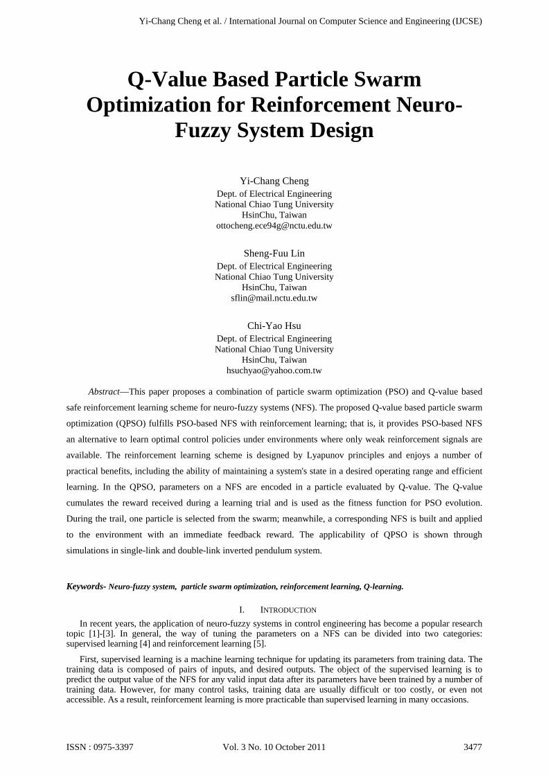
( ) ( ) ( 1) ... ( )R t r t r t r tγ γ Τ= + ⋅ + + + ⋅ + Τ , (13) where γ (0 ≤ γ ≤ 1) is the discount rate and T is the terminal time step. T usually refers to the end of an trial or, in a non-episodic task, infinity. The structure of Q-learning is shown in Fig. 1. An agent applies an action a(t) to the environment at a particular state x(t), causing a transition from x(t) to x(t+1) with an immediate reward r(t+1) in return. Then, the Q-function estimates the cumulative reward and is denoted by the Q-value of state-action pair (x(t), a(t)). The Q-value of each state-action pair is updated as follows:

*

*

' ( ( 1))

( ( ), ( )) ( ( ), ( )) [ ( 1) ( ( 1)) ( ( ), ( ))],( ( 1)) max ( ( 1), '),

a A x t

Q x t a t Q x t a t r t Q x t Q x t a t

Q x t Q x t a

α γ

∈ +

← + + + + −+ = +

(14)

where A(x(t+1)) is the set of candidate actions in state x(t+1) and α (0 ≤ α ≤ 1) is the learning rate.

Figure 1. Structure of Q-learning.

III. LYAPUNOV DESIGN OF LEARNING AAGGENTS Lyapunov design methods are widely used to achieve some commonly stated goals for controlling a

system, such as stabilizing a system or maintaining a system's state in a desired operating range. Lyapunov function is a scalar function of the system state and it often corresponds to some real, natural notion of energy in physical systems. The basic concept of Lyapunov function has been extended to reinforcement learning problems by Perkins and Barto [23]. The purpose of [23] is to guide the system to reach and remain in a set of goal states.

The proposed QPSO conducts one Lyapunov-style theorem proposed in [23], which provides a criterion for designing the reinforcement learning agent. The theorem is listed below. Let :L S → denotes a function positive on Tc=S-T, and Δ denotes a fixed real number. Theorem 1 If s T∀ ∉ , actions a∈A(s), all possible next state s' (either 's T∈ or ( ) ( ')L s L s− ≥ Δ ), then from

any ts T∉ , the environment enters T within ( ) /tL s Δ time steps. The proof of theorem 1 can be found in [23]. Theorem 1 provides a guarantee of a plant's meeting the goal

state, if the controller is designed such that it reduces the Lyapunov function of the plant in each time step. Therefore, the central task of the proposed QPSO is to identify a Lyapunov function of a control plant then design the action choices so that the reinforcement learning satisfies the above theorem. We also modify the original Q-learning algorithm into (15) so that the Q-value of a particle can indicate how soon the system's state entering the goal state:



*

*

' ( ( 1))

1( ( ), ( )) ( ( ), ( )) [ ( ( 1)) ( ( ), ( ))],

( ( 1)) max ( ( 1), ').a A x t

Q x t a t Q x t a t Q x t Q x t a tt

Q x t Q x t a

α γ

∈ +

← + − + + −

+ = + (15)

IV. THE LEARNING ALGORITHM OF QPSO Thorough learning algorithm of QPSO is described in this section. The architecture is shown in Fig.2. The

whole learning process can be roughly divided into two parts: the Q-value and PSO operation part. The learning strategy for Q-values of particles is detailed in section IV.A while the PSO operation and the flowchart of QPSO are described in section IV.B.

Figure 2. Architecture of QPSO

Finally, complete content and organizational editing before formatting. Please take note of the following items

when proofreading spelling and grammar:

A. Learning Q-values of Particles

In QPSO learning, if there are s particles in the swarm, s trials are taken in one generation. The agent applies in each trial an action to the environment by selecting a particle based on its Q-value. Every time a particle is selected, the Q-value of the selected particle is updated based on the system’s reward. As derived in (15), if the i -th particle is selected, its Q-value qi is updated as

*1( ) ( ) [ ( ( 1)) ( )], for 1, , , i i iq t q t Q x t q t i st

α γ= + − + + − = (16)

where *

*

' ( ( 1)) 1... 1...( ( 1)) max ( ( 1), ') max ( ( 1), ) max ( ) ( )i i ia A x t i s i s

Q x t Q x t a Q x t p q t q t∈ + = =

+ = + = + = = ; (17)

that is,

*

1( ) ( ) [ ( ) ( )] ( ) ( ), for 1, , ,i i i i iiq t q t q t q t q t t i s

tα γ αδ= + − + − = + = (18)

where δi(t) is regarded as TD error. The new Q-values of all particles calculated from (18) are subsequently adopted as the fitness values for PSO evolution.

B. Q-value Based PSO

The PSO operation used in QPSO consists of two major steps: swarm initialization and Q-valued base PSO evolution. Details of these two steps are described step-by step as follows.

• Swarm initialization

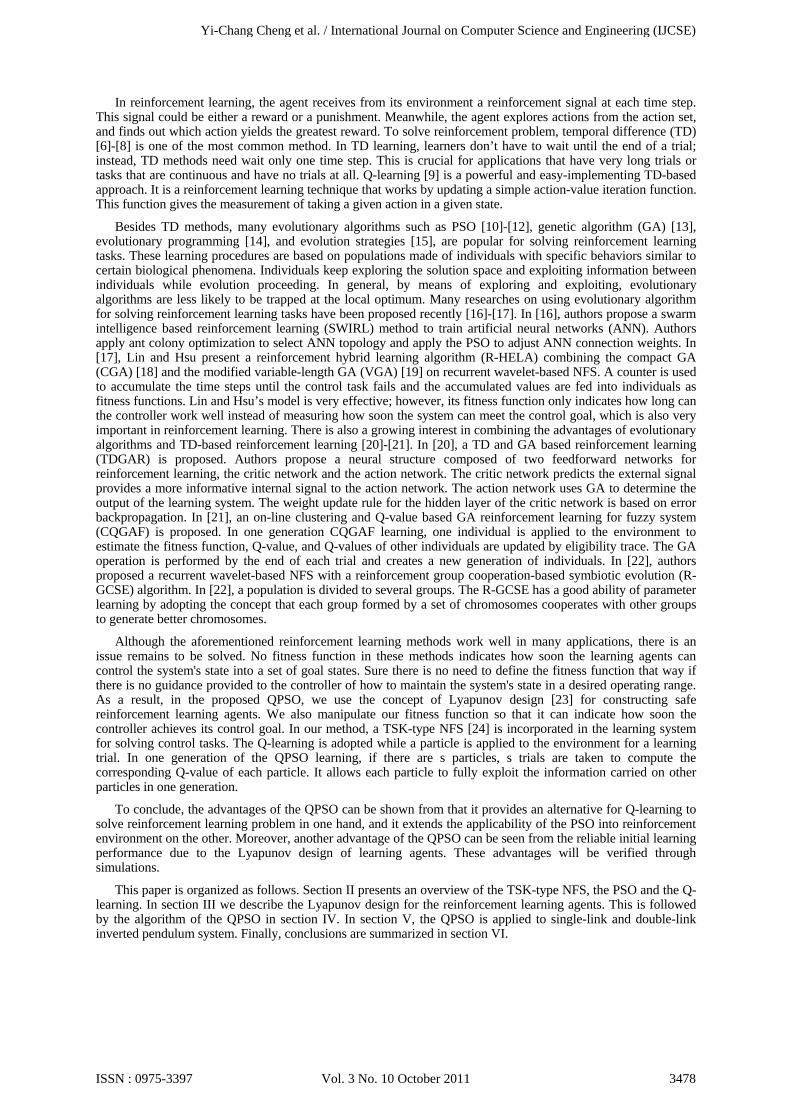
The particle swarm is composed of particles encoded by the parameters on a NFS. Each particle is encoded by the mean, deviation of Gaussian membership functions and the weightings for output action strength. The number of fuzzy rules determines the length of each particle. After the number of rules is set, the initial particles are generated according to the following equations:

[ ] [ ]min maxMean: , ,ip n random m m= (19)

where n=1,3,…,2NR-1; i=1,2, …,s.



[ ] [ ]min maxDeviation: , ,ip n random σ σ= (20)

where n=2,4,…,2NR.

[ ] [ ], min maxWeight: , ,g cChr n random w w= (21)

where n=2NR, 2NR+1,…,D.

pi represents the i-th particle in the swarm; N represents the input dimension; R represents the number of fuzzy rules; D represents the size of each particle, usually D equals to (N+1)R in most of cases where the dimension of output variable is 1; [mmin,,mmax], [σmin,,σmax] and [wmin,,wmax], are the predefined ranges. The above equations result in the coding scheme between a neural fuzzy system and a particle shown in Fig. 3.

Figure 3. Coding scheme between a particle and a TSK-type NFS in QPSO.

• Q-value based PSO evolution

The Q-values derived in (18) are used as the fitness values for PSO evolution. The Q-value of each particle determines the performance of a particle for controlling the system. In the proposed QPSO, the Q-value of each particle indicates how soon a particle can guide the system’s state to reach the set of goal states. The flowchart of how each particle evolves by the end of each trial is shown in Fig. 4 where q() represents the function to estimate a particle’s Q-value and max_gen represents the allowance number of generations that PSO evolution runs before meeting the stopping criteria.



Fig. 4. Flowchart of Q-valued based PSO evolution.

The learning processes of III.A and III.B proceeds to new generation until a predefined stop criterion is met. The block diagram of whole learning process in QPSO is shown in Fig. 5.

Fig. 5. Block diagram of QPSO.



V. ILLUSTRATIVE EXAMPLES Two simulations are discussed in this section. The first simulation is the cart-pole balance control [25] and

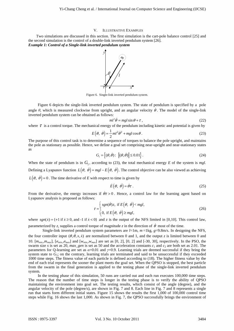
the second simulation is the control of a double-link inverted pendulum system [26]. Example 1: Control of a Single-link inverted pendulum system

Figure 6. Single-link inverted pendulum system.

Figure 6 depicts the single-link inverted pendulum system. The state of pendulum is specified by a pole

angle θ, which is measured clockwise from upright, and an angular velocity θ . The model of the single-link inverted pendulum system can be obtained as follows:

2 sinml mglθ θ τ= + , (22) where τ is a control torque. The mechanical energy of the pendulum including kinetic and potential is given by

( ) 2 21, cos2

E ml mglθ θ θ θ= + . (23)

The purpose of this control task is to determine a sequence of torques to balance the pole upright, and maintains the pole as stationary as possible. Hence, we define a goal set comprising near-upright and near-stationary states as

{ }1 ( , ) : ( , ) 0.01G θ θ θ θ= ≤ . (24)

When the state of pendulum is in 1G , according to (23), the total mechanical energy E of the system is mgl.

Defining a Lyapunov function ( ) ( ), , L mgl Eθ θ θ θ= − . The control objective can be also viewed as achieving

( ), 0L θ θ = . The time derivative of E with respect to time is given by

( ), E θ θ θτ= . (25)

From the derivative, the energy increases if 0θτ > . Hence, a control law for the learning agent based on Lyapunov analysis is proposed as follows:

( )( )

( ) , if , < ,

0, if , ,

sgn z E mgl

E mgl

θ θ θτ

θ θ

=

≥

(26)

where ( ) { 1 if 0, and -1 if 0}sgn x x x= + ≥ < and z is the output of the NFS limited in [0,10]. This control law, parameterized by z, supplies a control torque of magnitude z in the direction of θ most of the time. Single-link inverted pendulum system parameters are l=1m, m =1kg, g=9.8m/s. In designing the NFS, the four controller input ( , , , )x xθ θ are normalized between 0 and 1, and the output z is limited between 0 and 10. [mmin,,mmax], [σmin,,σmax] and [wmin,,wmax] are set as [0, 2], [0, 2] and [-30, 30], respectively. In the PSO, the swarm size s is set as 20, max_gen is set as 50 and the acceleration constants c1 and c2 are both set as 2.01. The parameters for Q-learning are set as α=0.01 and γ=0.9. Learning trials are deemed successful if they bring the system state to G1; on the contrary, learning trials are terminated and said to be unsuccessful if they exceeded 1000 time steps. The fitness value of each particle is defined according to (18). The higher fitness value by the end of each trial represents the sooner the plant meets the goal set. When the QPSO is stopped, the best particle from the swarm in the final generation is applied to the testing phase of the single-link inverted pendulum system.

In the testing phase of this simulation, 50 runs are carried out and each run executes 100,000 time steps. The reason that the number of time steps is longer in the testing phase is to verify the ability of QPSO maintaining the environment into goal set. The testing results, which consist of the angle (degree), and the angular velocity of the pole (degree/s), are shown in Fig. 7 and 8. Each line in Fig. 7 and 8 represents a single run that starts form different initial states. Figure 15 shows the results the first 1,000 of 100,000 control time steps while Fig. 16 shows the last 1,000. As shown in Fig. 7, the QPSO successfully brings the environment of



single-link inverted pendulum system to goal set G1 in all 50 runs. From Fig. 7 we can see that with the aid of Lyapunov design, the QPSO is able to control the single-link inverted pendulum system well under different initial conditions. Trajectories shown in Fig. 8 verify the ability of the QPSO marinating the environment into G1.

(a) (b)

Figure 7. First 1000 time steps control results of the single-link inverted pendulum system. (a) Angle of the pendulum. (b) Angular velocity of the pendulum.

(a) (b)

Figure 8. Last 1000 time steps control results of the single-link inverted pendulum system. (a) Angle of the pendulum. (b) Angular velocity of the pendulum.

To verify with the performance of the QPSO, the TD and GA based reinforcement learning (TDGAR) [20], the on-line clustering and Q-value based GA reinforcement learning (CQGAF) [21] and the recurrent wavelet-based NFS with a reinforcement group cooperation-based symbiotic evolution (R-GCSE) algorithm [22] are applied to the same control task. In the TDGAR, there are five hidden nodes and five rules in the critic network and the action network. The population size is set as 200 and the maximum perturbation is set as 0.0005. In the CQGAF, after trial-and-error tests, the final average number of rules from 50 runs was 6 by using the on-line clustering algorithm. The population size is set as 20. The parameters for Q-learning are set as α=0.01, λ=0.9 and γ=0.9. In the R-GCSE, the population size is set as 30 and the mutation rate is set as 0.01. In the QPSO and the compared approaches, a trail begins at a near upright state (5°,0, 0, 0) and ends when the control goal is met or a failure occurs. The control goal in this performance comparison test is defined as “bringing the plant to G1 and maintaining it for 10000 time steps.” A failure learning trial occurs if it exceeded 100000 time steps or the pendulum deviates beyond the range of ± 12°.

TABLE I. SUMMARY STATISTICS FOR EXAMPLE 1.

Methods QPSO TDGAR CQGAF R-GCSE

% of first 10% trials meeting goal. 96 56 70 78

% of trials meeting goal. 98 84 90 94

Time to goal, first 10% trials. 24.2 ± 0.8 200.2 ± 18.1 50.6 ± 7.2 78.9 ± 8.8

Average Time to goal. 21.6 ± 0.3 169.8 ± 12.9 34.2 ± 6.1 46.1 ± 4.9

The performances of all these compared methods are shown in Table I, from which we can see that the

QPSO has the successful control rate and requires the least CPU-time cost. The superiority can be seen especially from the first 10% learning trials where learning agents are not fully trained yet. This is one of the



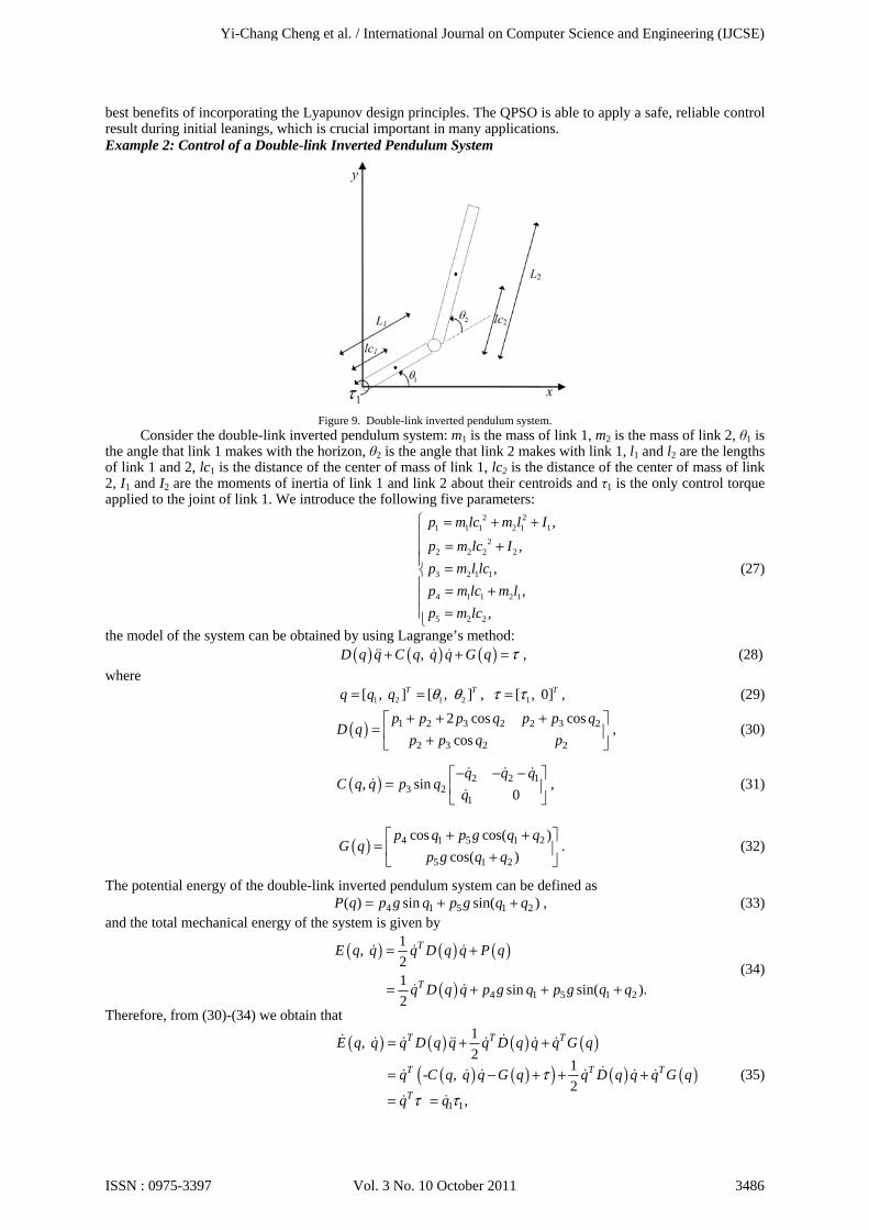
best benefits of incorporating the Lyapunov design principles. The QPSO is able to apply a safe, reliable control result during initial leanings, which is crucial important in many applications. Example 2: Control of a Double-link Inverted Pendulum System

Figure 9. Double-link inverted pendulum system.

Consider the double-link inverted pendulum system: m1 is the mass of link 1, m2 is the mass of link 2, θ1 is the angle that link 1 makes with the horizon, θ2 is the angle that link 2 makes with link 1, l1 and l2 are the lengths of link 1 and 2, lc1 is the distance of the center of mass of link 1, lc2 is the distance of the center of mass of link 2, I1 and I2 are the moments of inertia of link 1 and link 2 about their centroids and τ1 is the only control torque applied to the joint of link 1. We introduce the following five parameters:

2 21 1 1 2 1 1

22 2 2 2

3 2 1 1

4 1 1 2 1

5 2 2

,

,,

,,

p m lc m l I

p m lc I

p m l lc

p m lc m l

p m lc

= + +

= + = = + =

(27)

the model of the system can be obtained by using Lagrange’s method: ( ) ( ) ( ), D q q C q q q G q τ+ + = , (28)

where 1 2 1 2[ , ] [ , ]T Tq q q θ θ= = , 1[ , 0]Tτ τ= , (29)

( ) 1 2 3 2 2 3 2

2 3 2 2

2 cos coscos

p p p q p p qD q

p p q p

+ + + = +

, (30)

( ) 2 2 13 2

1, sin

0q q q

C q q p qq

− − − =

, (31)

( ) 4 1 5 1 2

5 1 2

cos cos( )cos( )

p q p g q qG q

p g q q

+ + = +

. (32)

The potential energy of the double-link inverted pendulum system can be defined as 4 1 5 1 2( ) sin sin( )P q p g q p g q q= + + , (33)

and the total mechanical energy of the system is given by

( ) ( ) ( )

( ) 4 1 5 1 2

1, 21 sin sin( ).2

T

T

E q q q D q q P q

q D q q p g q p g q q

= +

= + + +

(34)

Therefore, from (30)-(34) we obtain that

( ) ( ) ( ) ( )( ) ( )( ) ( ) ( )

1 1

1, 2

1- , 2

,

T T T

T T T

T

E q q q D q q q D q q q G q

q C q q q G q q D q q q G q

q q

τ

τ τ

= + +

= − + + +

= =

(35)



which shows the derivative of E is proportional to the product of the angular velocity of link 1 and the input torque. The control objective is to stabilize the system around its top position, i.e. 1 1 2 2( , , , )q q q q =(π/2,0,0,0). Denote 1 1 / 2q q π= − , another goal set is defined by

{ }2 1 1 2 2 1 1 2 2( , , , ) : ( , , , ) 0.01G q q q q q q q q= ≤ . (36) When the state of double-link inverted pendulum system is in G2, the total mechanical energy E of the system is given by

E(π/2, 0, 0, 0) = Etop = (p4+p5)g. (37)

By defining a Lyapunov function ( ) ( ) 2top

1, , 2

L q q E q q E = − , the control objective can be either considered

as guiding the system state into G2 or achieving ( ), 0L q q = . Hence in this paper, a control law for the learning agent in this example is proposed as follows:

( )( )

1 top1

top

( ) , if , < ,

0, if , ,

sgn q z E q q E

E q q Eτ

= ≥

(38)

where z is the output of the NFS limited in [0,10]. Double-link inverted pendulum system parameters are L1=1m, L2=2m, m1=1kg, m2=2kg, g=9.8m/s. In designing the NFS, the four controller input ),,,( xx θθ are normalized between 0 and 1, the output z is limited between 0 and 10. [mmin,,mmax], [σmin,,σmax] and [wmin,,wmax] are set as [0,2], [0,2] and [-30,30], respectively. In the PSO, the swarm size s is set as 40, max_gen is set as 50 and the acceleration constants c1 and c2 are both set as 2.01. The parameters for Q-learning are set as α=0.01 and γ=0.9. Learning trials are deemed successful if they bring the plant to G2; on the contrary, learning trials are terminated and said to be unsuccessful if they exceeded 1000 time steps. When the QPSO is stopped, the best particle from the swarm in the final generation is applied to the testing phase of the single-link inverted pendulum system.

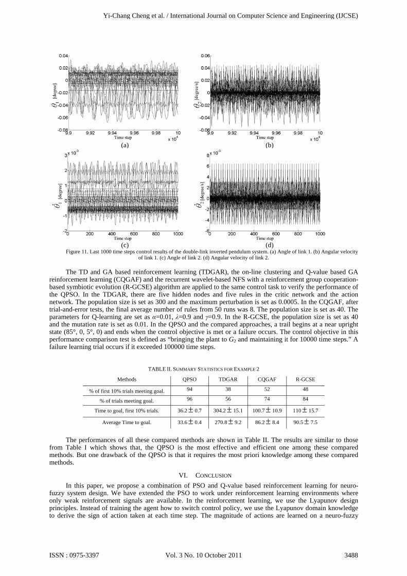
In the testing phase of this simulation, 50 runs are carried out and each run executes 100,000 time steps. The testing results, which consist of the angle (degree) and the angular velocity (degree/s) of link 1 and link 2, are shown in Fig. 10 and 11. Figure 10 shows the results the first 1,000 of 100,000 control time steps while Fig. 11 shows the last 1,000. As shown in Fig. 10, the QPSO successfully brings the environment of double-link inverted pendulum system to goal set G2 in all 50 runs under different initial environments. Trajectories shown in Fig. 11 verify the ability of the QPSO marinating the environment into G2.

(a) (b)

(c) (d)

Figure 10. First 1000 time steps control results of the double-link inverted pendulum system. (a) Angle of link 1. (b) Angular velocity of link 1. (c) Angle of link 2. (d) Angular velocity of link 2.



(a) (b)

(c) (d)

Figure 11. Last 1000 time steps control results of the double-link inverted pendulum system. (a) Angle of link 1. (b) Angular velocity of link 1. (c) Angle of link 2. (d) Angular velocity of link 2.

The TD and GA based reinforcement learning (TDGAR), the on-line clustering and Q-value based GA

reinforcement learning (CQGAF) and the recurrent wavelet-based NFS with a reinforcement group cooperation-based symbiotic evolution (R-GCSE) algorithm are applied to the same control task to verify the performance of the QPSO. In the TDGAR, there are five hidden nodes and five rules in the critic network and the action network. The population size is set as 300 and the maximum perturbation is set as 0.0005. In the CQGAF, after trial-and-error tests, the final average number of rules from 50 runs was 8. The population size is set as 40. The parameters for Q-learning are set as α=0.01, λ=0.9 and γ=0.9. In the R-GCSE, the population size is set as 40 and the mutation rate is set as 0.01. In the QPSO and the compared approaches, a trail begins at a near upright state (85°, 0, 5°, 0) and ends when the control objective is met or a failure occurs. The control objective in this performance comparison test is defined as “bringing the plant to G2 and maintaining it for 10000 time steps.” A failure learning trial occurs if it exceeded 100000 time steps.

TABLE II. SUMMARY STATISTICS FOR EXAMPLE 2

Methods QPSO TDGAR CQGAF R-GCSE

% of first 10% trials meeting goal. 94 38 52 48

% of trials meeting goal. 96 56 74 84

Time to goal, first 10% trials. 36.2 ± 0.7 304.2 ± 15.1 100.7 ± 10.9 110 ± 15.7

Average Time to goal. 33.6 ± 0.4 270.8 ± 9.2 86.2 ± 8.4 90.5 ± 7.5

The performances of all these compared methods are shown in Table II. The results are similar to those

from Table I which shows that, the QPSO is the most effective and efficient one among these compared methods. But one drawback of the QPSO is that it requires the most priori knowledge among these compared methods.

VI. CONCLUSION In this paper, we propose a combination of PSO and Q-value based reinforcement learning for neuro-

fuzzy system design. We have extended the PSO to work under reinforcement learning environments where only weak reinforcement signals are available. In the reinforcement learning, we use the Lyapunov design principles. Instead of training the agent how to switch control policy, we use the Lyapunov domain knowledge to derive the sign of action taken at each time step. The magnitude of actions are learned on a neuro-fuzzy



system trained by PSO. With the assistance of Lyapunov design, the QPSO can enjoy several qualitative objectives. The simulations also verify the feasibility and efficiency of the proposed QPSO.

REFERENCES [1] J. J. Buckley and Y. Hayashi, “Neural nets for fuzzy-systems,” Fuzzy Sets And System, vol. 71, no. 3, pp. 265-276, May 1995. [2] G. G. Towell and J. W. Shavlik, “Extracting refined rules from knowledge-based neural networks,” Machine Learning, vol. 13, pp. 71-

101, 1993. [4] R. Caruana and A. Niculescu-Mizil, “An Empirical Comparison of Supervised Learning Algorithms,” Proc. Int. Conf. Machine

Learning, pp. 161-168 , 2006. [5] R. S. Sutton and A. G. Barto, Reinforcement learning. Cambridge, MA: MIT Press, 1998. [6] J. N. Tsitsiklis and B. V. Roy, “An analysis of temporal-difference with function approximation,” IEEE Trans. Autom. Control, vol.

42, no. 5, pp. 834-836, Sep. 1983 [7] C. J. Wakins, “Learning from delayed rewards,” Ph.D. dissertation, King’s College, Cambridge, U.K., 1989. [8] E. BARNARD, “Temporal-difference methods and Markov models,” IEEE Trans. on Systems Man and Cybernetics, vol. 23, Issue: 2

pp. 357-365, 1993 [9] C. J.Wakins and P. Dayan, “Technical note: Q-learning,” Machine Learning, vol. 8, pp. 279–292, 1992. [10] J. Kennedy and R. C. Eberhart, “Particle Swarm Optimization,” in Proc. of IEEE Int. Conf. on Neural Networks, vol. 4, pp. 1942-1948,

1995. [11] F. Bergh and A. P. Engelbrecht, “A Cooperative Approach to Particle Swarm Optimization,” IEEE Trans. on Evolutionary

Computation, vol. 8, no. 3, pp. 58-73, 2002. [12] M. Clerc and J. Kennedy, “The Particle Swarm—Explosion, Stability, and Convergence in a Multidimensional Complex Space,” IEEE

Trans. on Evolutionary Computation, vol. 6, no. 1, pp. 225-239, 2004. [13] D. E. Goldberg, Genetic Algorithms in Search Optimization and Machine Learning. Reading, MA: Addison-Wesley, 1989. [14] L. J. Fogel, “Evolutionary programming in perspective: The top-down view,” in Computational Intelligence: Imitating Life, J. M.

Zurada, R. J. Marks II, and C. Goldberg, Eds. Piscataway, NJ: IEEE Press, 1994. [15] I. Rechenberg, “Evolution strategy,” in Computational Intelligence: Imitating Life, J. M. Zurada, R. J. Marks II, and C. Goldberg, Eds.

Piscataway, NJ: IEEE Press, 1994. [16] M. Conforth and Y. Meng, “Reinforcement Learning for Neural Networks using swarm Intelligence,” IEEE Swarm Intelligence

Symposium, pp. 7, 2008 [17] C. J. Lin and Y. C. Hsu, “Reinforcement Hybrid Evolutionary Learning for Recurrent Wavelet-Based Neuro-Fuzzy Systems,” IEEE

Trans. Fuzzy Systs., vol. 15, no. 4, 2007, pp. 729-745. [18] G. R. Harik, F. G. Lobo, and D. E. Goldberg, “The compact genetic algorithm,” IEEE Trans. on Evolutionary Computation, vol. 3, pp.

287–297, Nov. 1999. [19] S. Bandyopadhyay, C. A. Murthy, and S. K. Pal, “VGA-classifier: design and applications,” IEEE Trans. on Systems Man and

Cybernetics, Part B, vol. 30, no. 6, pp. 890–895, 2000. [20] C. T. Lin and C. P. Jou, “GA-based fuzzy reinforcement learning for control of a magnetic bearing system,” IEEE Trans. on Systems

Man and Cybernetics, Part B, vol. 30, no. 2, pp. 276-289, 2000. [21] C. F. Juang, “Combination of online clustering and Q-value based GA for reinforcement fuzzy system design,” IEEE Trans. on Fuzzy

Systs., vol. 13, no. 3, pp. 289–302, 2005. [22] Y.C. Hsu and S.F. Lin, “Reinforcement Group Cooperation based Symbiotic Evolution for Recurrent Wavelet-Based Neuro-Fuzzy

Systems,” Neurocomputing, vol. 72, no. 10-12, pp. 2418-2432, 2009. [23] Perkins, T.J. and A.G. Barto, “Lyapunov design for safe reinforcement learning.” Journal of Machine Learning Research, 2003. 3(4-5):

p. 803-832. [24] Takagi, T. and M. Sugeno, “Fuzzy Identification of Systems and Its Applications to Modeling and Control,” IEEE Trans. on Systems

Man and Cybernetics, 1985. 15(1): p. 116-132. [25] K. Furuta and M. Iwase, “Swing-up time analysis of pendulum,” Bulletin of the Polish Academy of Sciences - Technical Sciences, vol.

52, no. 3, pp. 153-163, 2004. [26] C. Popescu, “Nonlinear control of underactuated horizontal double pendulum,” M.S. thesis, University of Florida Atlantic, Boca Raton,

Florida, U.S., 2002.



q-value based particle swarm optimization for ... · q-value based particle swarm optimization for...

Documents