qc15 02 intro.ppt - isti.tu-berlin.de · stern-gerlach measurement video...
TRANSCRIPT

2
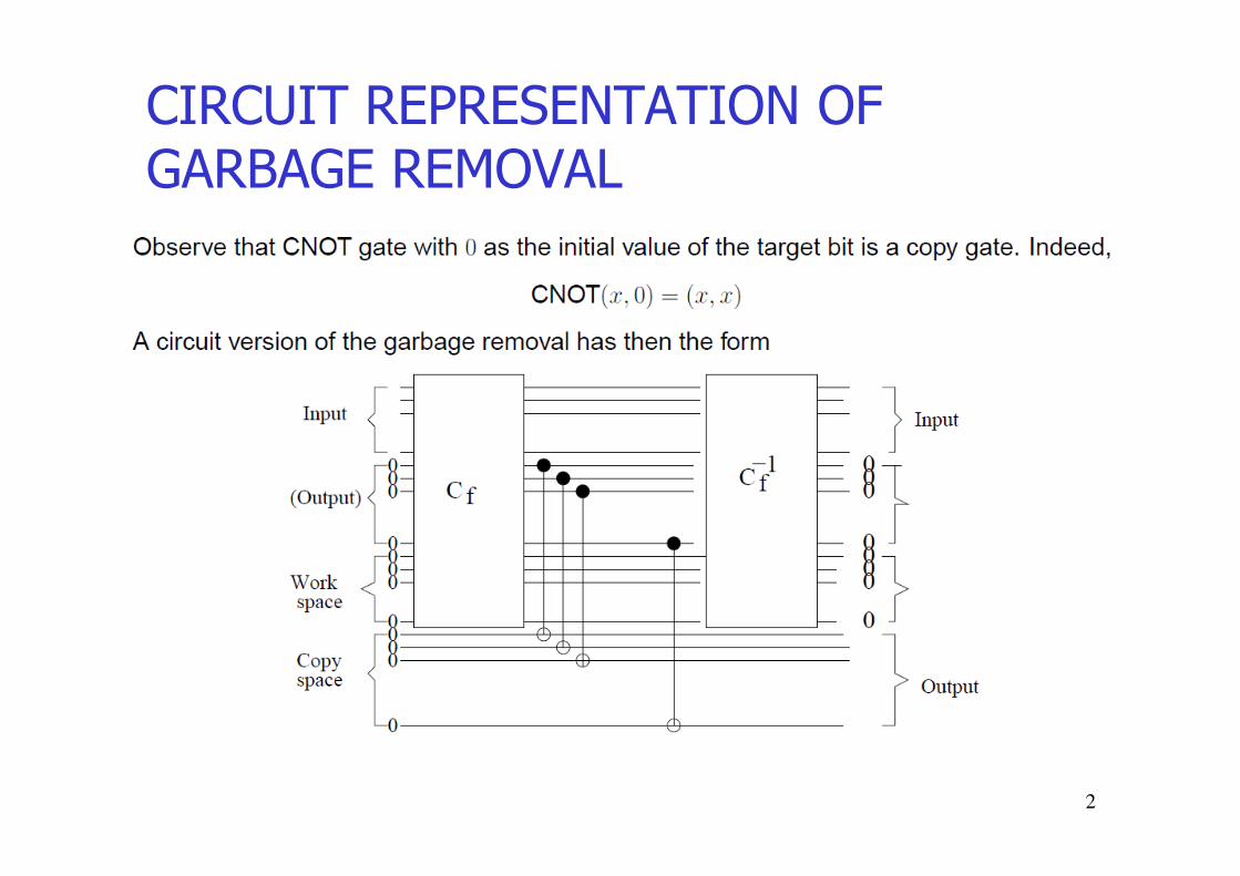
CIRCUIT REPRESENTATION OF GARBAGE REMOVAL

3
Outline for this lecture
Mathematics of Quantum Mechanics

4
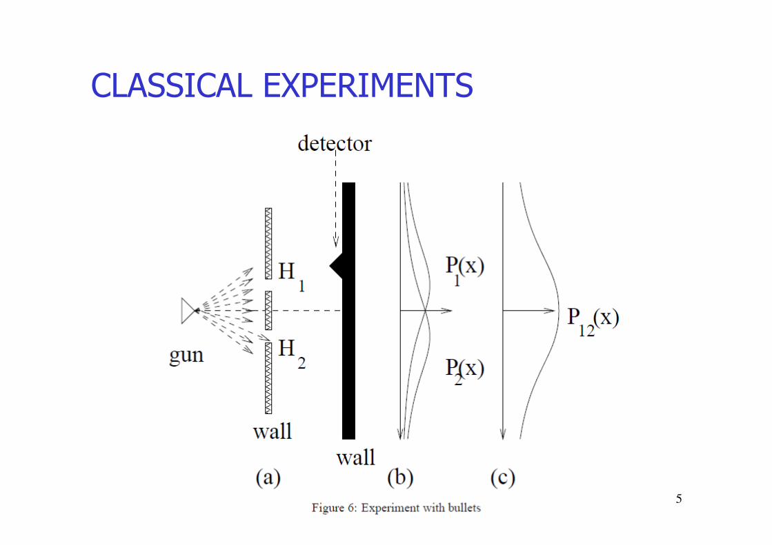
CLASSICAL EXPERIMENTS
5
CLASSICAL EXPERIMENTS

6
CLASSICAL EXPERIMENTS

7
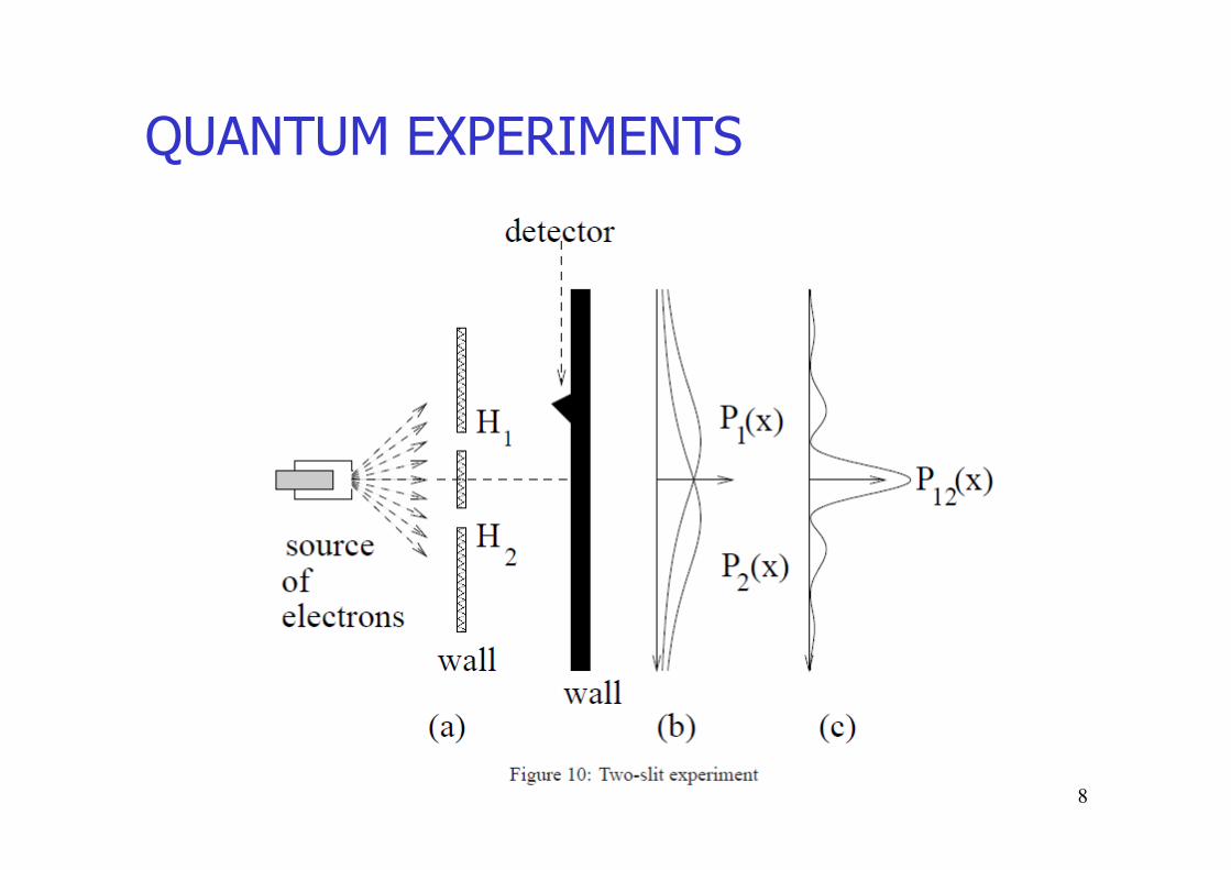
QUANTUM EXPERIMENTS
8
QUANTUM EXPERIMENTS
9
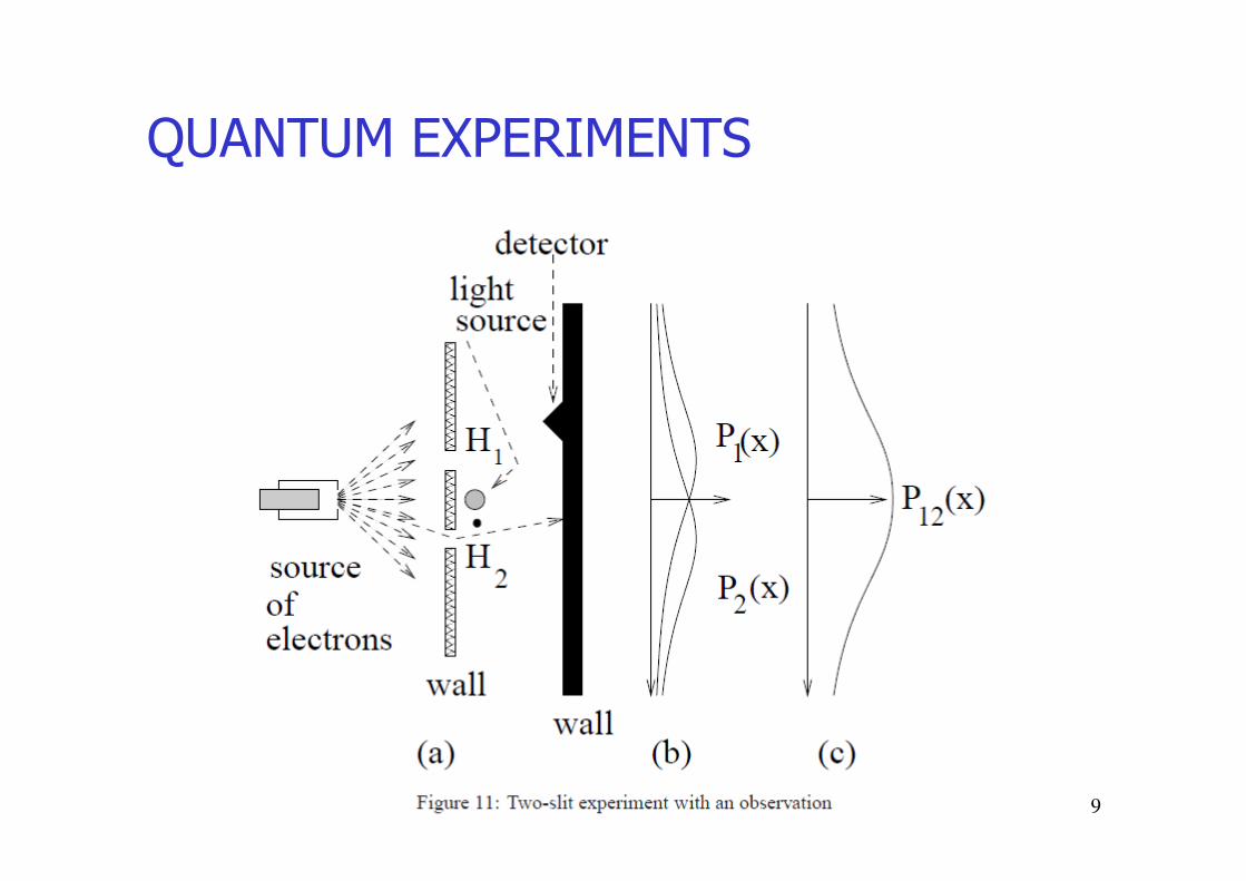
QUANTUM EXPERIMENTS

10
TWO-SLIT EXPERIMENT –OBSERVATIONS
r Contrary to our intuition, at some places one observes fewer
electrons when both slits are open, than in the case only one slit is
open.
r Electrons – particles, seem to behave as waves.
r Each electron seems to behave as going through both holes at
once.
r Results of the experiment do not depend on frequency with which
electrons are shot.
r Quantum physics has no explanation where a particular electron
reaches the detector wall. All quantum physics can offer are
statements on the probability that an electron reaches a certain
position on the detector wall.
11
BOHR’s WAVE-PARTICLE DUALITY PRINCIPLES
r Things we consider as waves correspond actually to
particles and things we consider as particles have waves
associated with them.
r The wave is associated with the position of a particle –
the particle is more likely to be found in places where its
wave is big.
r The distance between the peaks of the wave is related to
the particle’s speed; the smaller the distance, the faster
particle moves.
r The wave’s frequency is proportional to the particle’s
energy. (In fact, the particle’s energy is equal exactly to
its frequency times Planck’s constant.)

12
QUANTUM MECHANICS
r Quantum mechanics is a theory that describes atomic and
subatomic particles and their interactions.
r Quantum mechanics was born around 1925.
r A physical system consisting of one or more quantum particles is
called a quantum system.
r To completely describe a quantum particle an infinite-
dimensional Hilbert space is required.
r For quantum computational purposes it is sufficient to have a
partial description of particle(s) given in a finite-dimensional
Hilbert (inner-product) space.
r To each isolated quantum system we associate an inner-product
vector space elements of which norm-1 sates are called (pure)
states.
13
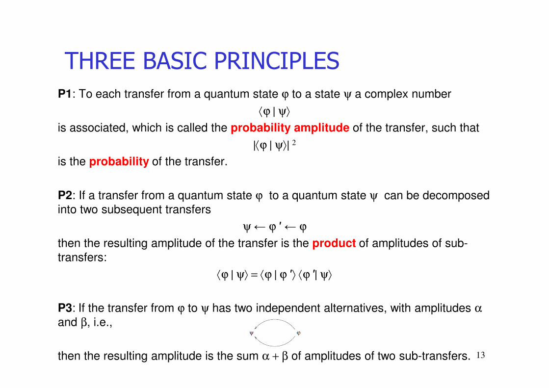
THREE BASIC PRINCIPLES
P1: To each transfer from a quantum state ϕ to a state ψ a complex number
⟨ϕ | ψ⟩
is associated, which is called the probability amplitude of the transfer, such that
|⟨ϕ | ψ⟩| 2
is the probability of the transfer.
P2: If a transfer from a quantum state ϕ to a quantum state ψ can be decomposed into two subsequent transfers
ψ ← ϕ ′ ← ϕ
then the resulting amplitude of the transfer is the product of amplitudes of sub-transfers:
⟨ϕ | ψ⟩ = ⟨ϕ | ϕ ′⟩ ⟨ϕ ′| ψ⟩
P3: If the transfer from ϕ to ψ has two independent alternatives, with amplitudes αand β, i.e.,
then the resulting amplitude is the sum α + β of amplitudes of two sub-transfers.
14
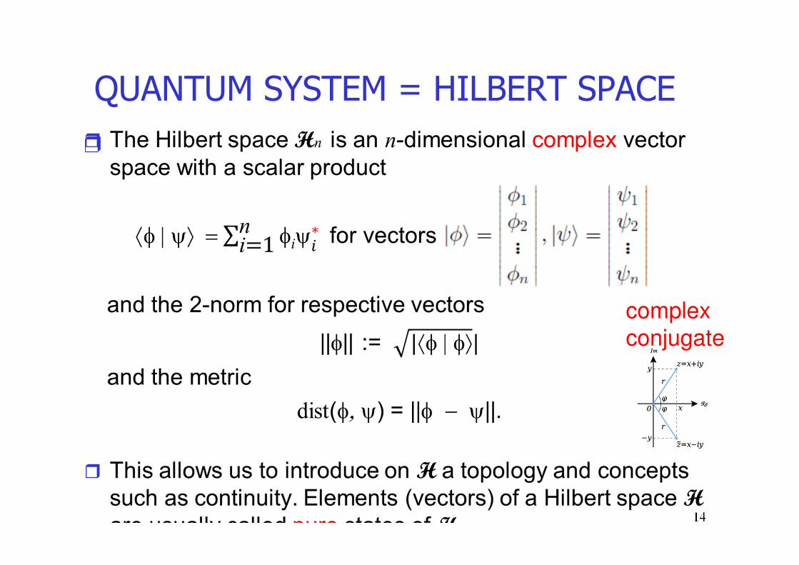
QUANTUM SYSTEM = HILBERT SPACE
r
complex conjugate

15
ORTHOGONALITY of PURE STATES
r Two quantum states | ψ⟩ and | φ⟩ are called orthogonal if their scalar product is zero, that is if
⟨φ | ψ⟩ = 0.
r Two pure quantum states are physically perfectly distinguishable only if they are orthogonal.
r In every Hilbert space there are so-called orthogonal bases all states of which are mutually orthogonal.
16
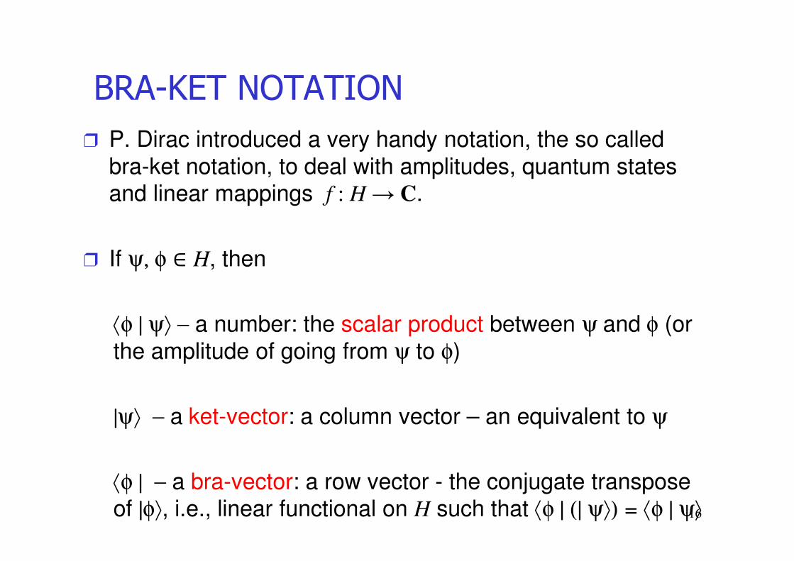
BRA-KET NOTATION
r P. Dirac introduced a very handy notation, the so called bra-ket notation, to deal with amplitudes, quantum states and linear mappings f : H→ C.
r If ψ, φ ∈ H, then
⟨φ | ψ⟩ − a number: the scalar product between ψ and φ (or the amplitude of going from ψ to φ)
|ψ⟩ − a ket-vector: a column vector – an equivalent to ψ
⟨φ | − a bra-vector: a row vector - the conjugate transpose of |φ⟩, i.e., linear functional on H such that ⟨φ | (| ψ⟩) = ⟨φ | ψ⟩
17
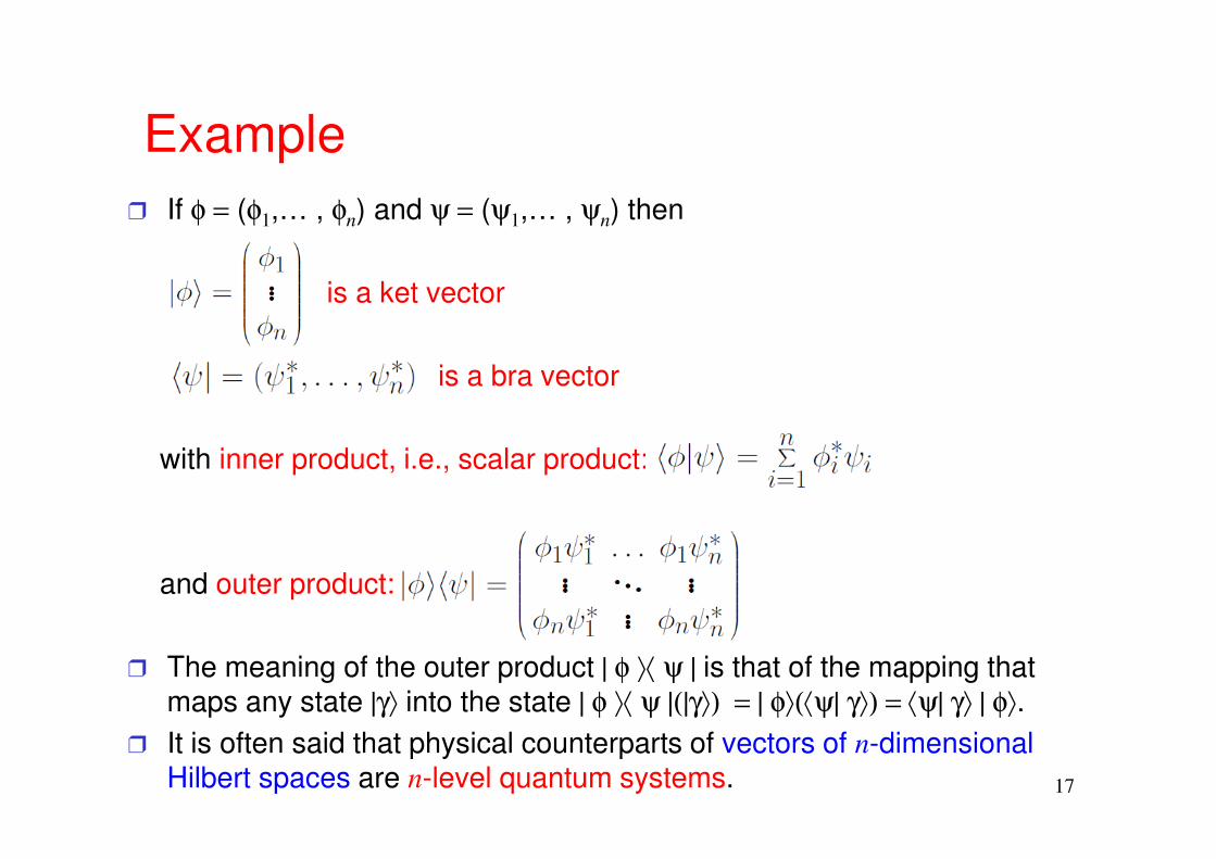
r If φ = (φ1,… , φn) and ψ = (ψ1,… , ψn) then
is a ket vector
is a bra vector
with inner product, i.e., scalar product:
and outer product:
r The meaning of the outer product | φ ⟩⟨ ψ | is that of the mapping that maps any state |γ⟩ into the state | φ ⟩⟨ ψ |(|γ⟩) = | φ⟩(⟨ψ| γ⟩) = ⟨ψ| γ⟩ | φ⟩.
r It is often said that physical counterparts of vectors of n-dimensional Hilbert spaces are n-level quantum systems.
Example

18
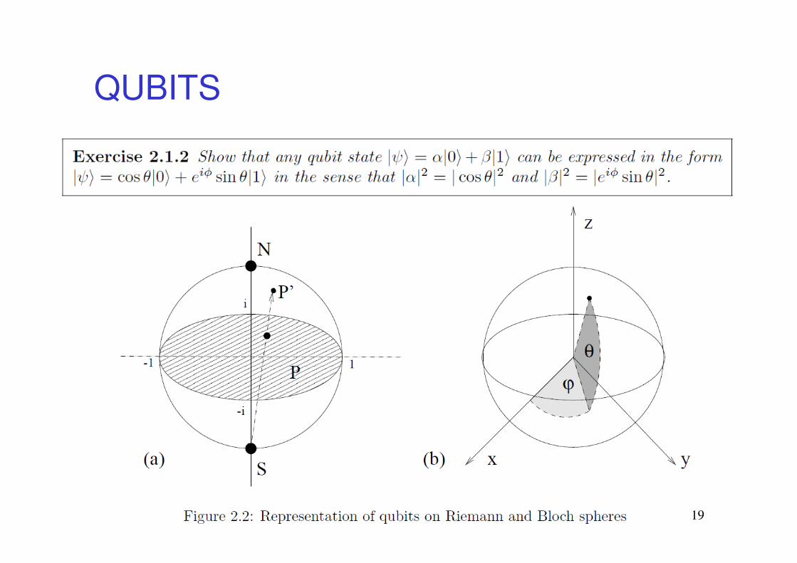
r A qubit – a two-level quantum system is a quantum state in H2
| φ ⟩ = α |0⟩ + β |1⟩
with α, β ∈ C are such that |α|2 + |β|2 = 1 and
{|0⟩, |1⟩}
some (standard) basis of H2.
r EXAMPLE: Representation of qubits by
(a) electron in a Hydrogen atom (b) a spin-1
QUBITS
19
QUBITS

20
The essence of the difference between
classical computers and quantum computers
is in the way information is stored and processed.
r In classical computers, information is represented on macroscopic level by
bits, which can take one of the two values
0 or 1.
r In quantum computers, information is represented on microscopic level using
qubits, which can take on any from uncountable many values
α |0⟩ + β |1⟩
with α, β ∈ C are such that
|α|2 + |β|2 = 1.
CLASSICAL vs. QUANTUM COMPUTING
21
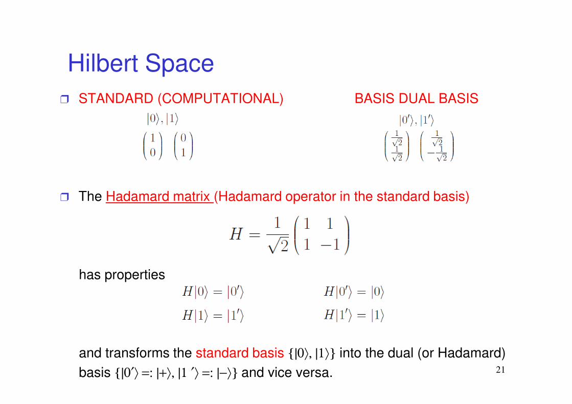
r STANDARD (COMPUTATIONAL) BASIS DUAL BASIS
r The Hadamard matrix (Hadamard operator in the standard basis)
has properties
and transforms the standard basis {|0⟩, |1⟩} into the dual (or Hadamard)
basis {|0′⟩ =: |+⟩, |1 ′⟩ =: |−⟩} and vice versa.
Hilbert Space
22
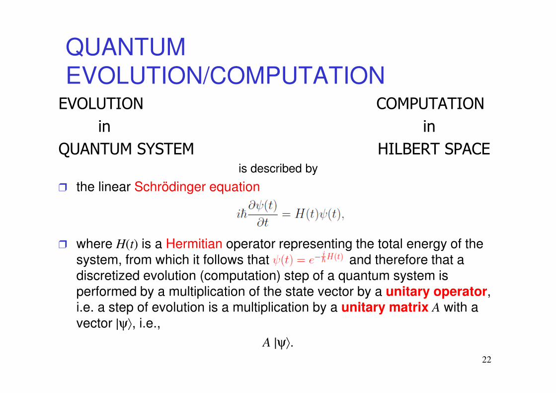
EVOLUTION COMPUTATION
in in
QUANTUM SYSTEM HILBERT SPACEis described by
r the linear Schrödinger equation
r where H(t) is a Hermitian operator representing the total energy of the system, from which it follows that and therefore that a discretized evolution (computation) step of a quantum system is performed by a multiplication of the state vector by a unitary operator, i.e. a step of evolution is a multiplication by a unitary matrix A with a vector |ψ⟩, i.e.,
A |ψ⟩.
QUANTUM EVOLUTION/COMPUTATION

23
Unitary Operator / Matrix

24
r The Schrödinger equation tells us how a quantum system
evolves
subject to the Hamiltonian.
r However, in order to do quantum mechanics, one has to know
how to pick up the Hamiltonian.
r The principles that tell us how to do so are real bridge
principles of quantum mechanics.
r Each quantum system is actually uniquely determined by a
Hamiltonian.
HAMILTONIANS

25
UNITARY MATRICES —EXAMPLES
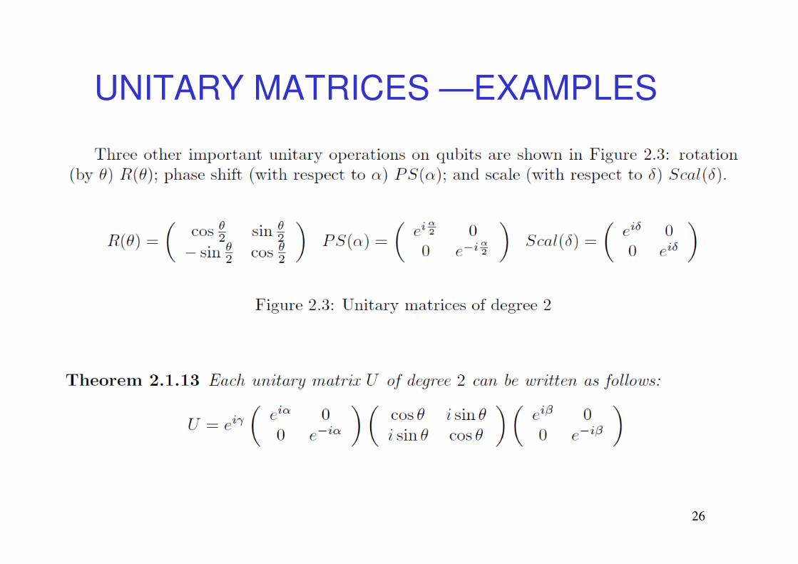
26
UNITARY MATRICES —EXAMPLES
27
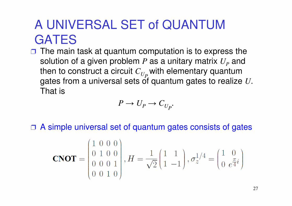
r The main task at quantum computation is to express the solution of a given problem P as a unitary matrix UP and then to construct a circuit CUP
with elementary quantum gates from a universal sets of quantum gates to realize U. That is
P → UP → CUP.
r A simple universal set of quantum gates consists of gates
A UNIVERSAL SET of QUANTUM GATES

28
For the Hamiltonian
the Schödinger equation
has the solution
and therefore for t = 1,
SOLVING SCHRÖDINGER’s EQUATION

29
r Let us consider, in an idealized form, one of the other famous experiments of quantum physics which demonstrates that some quantum phenomena are not determined except when they are measured.
r It was used to demonstrate that electrons and atoms have intrinsically quantum properties, and how measurement in quantum mechanics affects the system being measured.
STERN-GERLACH MEASUREMENT EXPERIMENT

30
r Specifically, the experiment demonstrates the property of spin and its quantized nature.
r Particles (silver atoms in the original experiment) are sent through an inhomogeneous magnetic field to hit a screen. Spin causes the particles to have a magnetic moment, and the magnetic field deflects the particles from their straight path. The screen shows discrete points rather than a continuous distribution, owing to the quantum nature of spin.
r The quantum theory explanation is the following one:
Passing an atom through a magnetic field amounts to a measurement of its magnetic alignment, and until you make such a measurement there is no sense in saying what the atom’s magnetic alignment might be; only when you make a measurement you obtain one of only two possible outcomes, with equal probability, and those two possibilities are defined by the direction of the magnetic field that you use to make the measurement.
STERN-GERLACH MEASUREMENT EXPERIMENT

31
STERN-GERLACH MEASUREMENT video
Quantum_spin_and_the_Stern-Gerlach_experiment.ogv
The Stern–Gerlach experiment was performed in Frankfurt, Germany in 1922 by Otto Stern and Walther Gerlach. At the time, Stern was an assistant to Max Born at the University of Frankfurt's Institute for Theoretical Physics, and Gerlach was an assistant at the same university's Institute for Experimental Physics.

32
r of vectors is
(φ1,...,φn)⊗(ψ1,...,ψm) = (φ1ψ1,..., φ1ψm, φ2ψ1,..., φ2ψm,..., φnψ1,..., φnψm)
r of matrices is
r of Hilbert spaces H,H′ is H⊗H′, i.e., the complex vector space spanned by tensor products of vectors from H and H′, that corresponds to the quantum system composed of the quantum systems corresponding to Hilbert spaces Hand H′.
r A very important difference between classical and quantum systems:
A state of a compound classical (quantum) system can be (cannot be) always composed from the states of its subsystems.
TENSOR PRODUCT
33
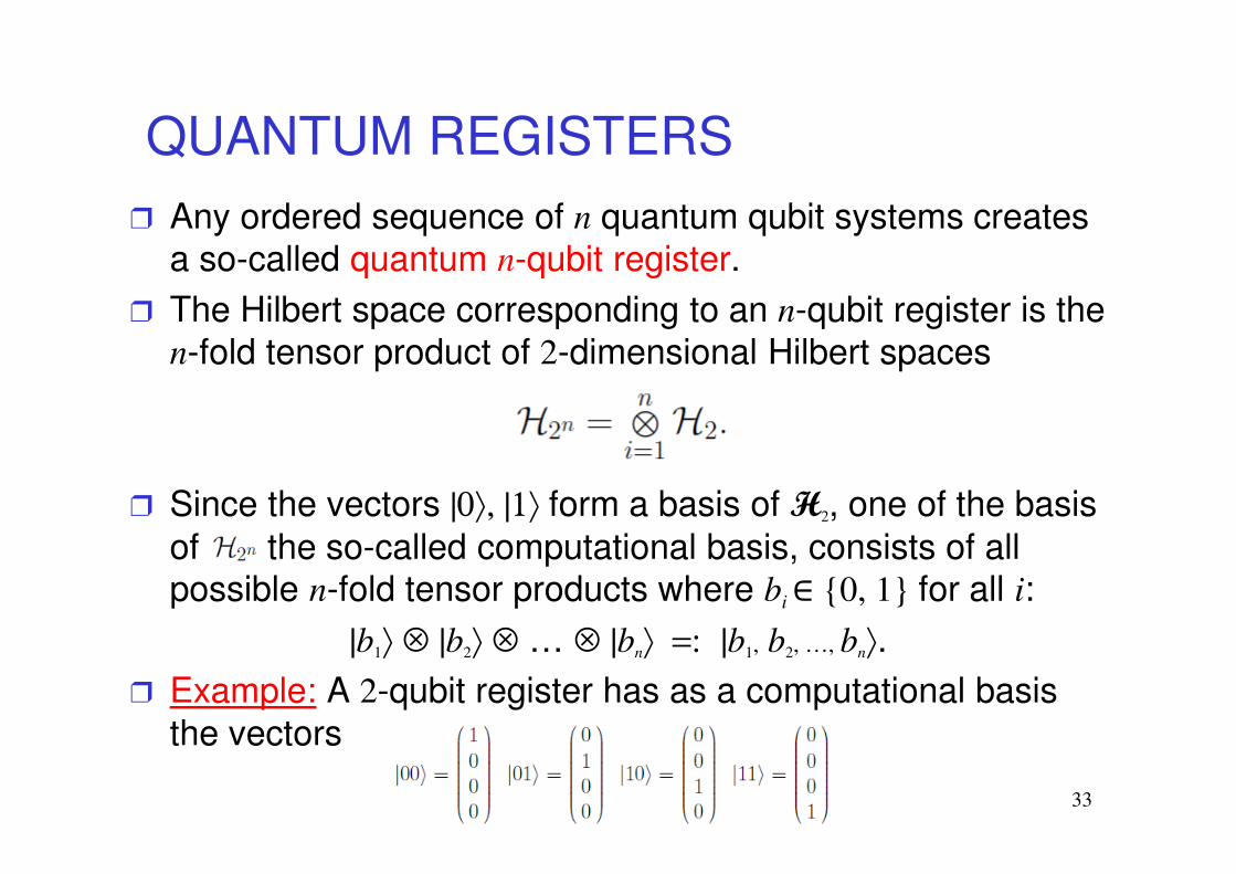
r Any ordered sequence of n quantum qubit systems creates a so-called quantum n-qubit register.
r The Hilbert space corresponding to an n-qubit register is the n-fold tensor product of 2-dimensional Hilbert spaces
r Since the vectors |0⟩, |1⟩ form a basis of H2, one of the basis of , the so-called computational basis, consists of all possible n-fold tensor products where bi∈ {0, 1} for all i:
|b1⟩ ⊗ |b2⟩ ⊗ … ⊗ |bn⟩ =: |b1, b2, …, bn⟩.
r Example: A 2-qubit register has as a computational basis the vectors
QUANTUM REGISTERS

34
QUANTUM STATES and von NEUMAN MEASUREMENTs
35
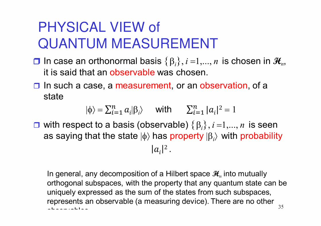
PHYSICAL VIEW of QUANTUM MEASUREMENT
r

36
r In so called “relative state interpretation” of quantum mechanics a
quantum state is interpreted as an objective real physical object.
r In so called “information view of quantum mechanics” a quantum
state is interpreted as a specification of (our knowledge or beliefs)
probabilities of all experiments that can be performed with the
state - the idea that quantum states describe the reality is therefore
abounded.
A quantum state is a useful abstraction which frequently appears in the literature, but does not really
exists in nature.
A. Peres (1993)
WHAT ARE ACTUALLY QUANTUM STATES? - TWO VIEWS
37
r A quantum state is observed (measured) with respect to an observable — a decomposition of a given Hilbert space into orthogonal subspaces (such that each vector can be uniquely represented as a sum of vectors of these subspaces).
r There are two outcomes of a projection measurement of a state |φ⟩:1. Classical information into which subspace projection of |φ⟩ was
made.
2. A new quantum state |φ′⟩ into which the state |φ⟩ collapses.
r The subspace into which projection is made is chosen randomly and the corresponding probability is uniquely determined by the amplitudes at the representation of |φ⟩ at the basis states of the subspace.
QUANTUM (PROJECTION) MEASUREMENTS
38
in CLASSICAL versus QUANTUM physics
r BEFORE QUANTUM PHYSICS it was taken for granted that
when physicists measure something, they are gaining knowledge
of a pre-existing state — a knowledge of an independent fact
about the world.
QUANTUM PHYSICS
r says otherwise. Things are not determined except when they are
measured, and it is only by being measured that they take on
specific values.
r A quantum measurement forces a previously indeterminate
system to take on a definite value.
MEASUREMENT
39
r Let us illustrate, on an example, a principal difference between a quantum evolution and a classical probabilistic evolution.
r If a qubit system develops under the evolution
r then, after one step of evolution, we observe both |0⟩ and |1⟩with the probability 1/2, but after two steps we get
r and therefore any observation gives |0⟩ with probability 1.
PROBABILISTIC vs. QUANTUM SYSTEM

40
r On the other hand, in case of the classical probabilistic evolution
r we have after one step of evolution both 0 and 1 with the same probability 1/2 but after two steps we have again
r and therefore, after two steps of evolution, we have again both values 0 and 1 with the same probability 1/2.
In the quantum case, during the second evolution step, amplitudes at |1⟩ cancel each other and we have so-called destructive interference. At the same time, amplitudes at |0⟩ amplify each other and we have so-called constructive interference.

41
Outline for next lecture
BASIC CONCEPTS and RESULTS

42
Questions?