qgen: quantitative genetics using r -...
TRANSCRIPT

qgen:quantitative genetics using R
Abstract
qgen is a collection of functions to analyse quantitative genetic data. It is especiallyhelpful to perform parametric resampling of quantitative genetic data sets. Resamplingallows first to determine a priori the expected variance of an estimator, second for agiven empirical data set to calculate bootstrap confidence intervals, and third to evaluatedifferent estimators and confidence intervals. The structure of the functions was kept“simple”which easily allows you to extend it with functions that calculate the statistics ofyour interest. The organisation of the functions together with some examples is describedin this document, for descriptions of the individual functions refer to the manual.
1 The basic organisation
Most functions in qgen are written to handle objects of class paraDATA (Figure 1).The name indicates that these objects can contain parameters sets as well as data sets.Nevertheless, in all standard applications they contain either a parameter set or a data setbut never both. The possibility of having both together allows to change this behavioureasily, e.g., to calculate non–parametric bootstrap estimates, where a new data set is notsimulated from parameters but sampled from an existing data set (Section 3).
Starting an investigation needs that you first transform your biological parameters oryour empirical data set into an object of class paraDATA. There are two functions to doexactly this job, the() and emp().
The functions est() and sim() do not only take paraDATA–objects as arguments butalso return paraDATA–objects. This allows to call these functions nested within eachother in a flexible way. For example
> my.paraDATA.object <- the()> est(sim(est(sim(est(sim(my.paraDATA.object))))))
1
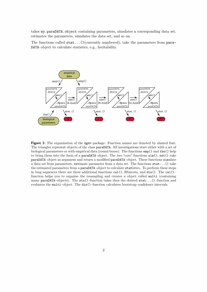
takes my.paraDATA.object containing parameters, simulates a corresponding data set,estimates the parameters, simulates the data set, and so on.
The functions called stat...()(currently numbered), take the parameters from para-DATA–object to calculate statistics, e.g., heritability.
biologicalparameters
empiricaldata
est()
emp()
sim()[S-fold]
est()
sim()[R-fold]
est()
sim()[Q-fold]
the()
tθ t* t**
stat..()stat..() stat..() stat..()
...@para ...@para ...@para ...@para
...@DATA...@DATA ...@DATAparaDATA paraDATA paraDATA
paraDATA paraDATA paraDATA paraDATA
est()...@DATAparaDATA
emp()
Figure 1: The organisation of the qgen–package: Function names are denoted by slanted font.The triangles represent objects of the class paraDATA. All investigations start either with a set ofbiological parameters or with empirical data (round boxes). The functions emp() and the() helpto bring them into the form of a paraDATA–object. The two “core” functions sim(), est() takeparaDATA–object as argument and return a modified paraDATA–object. These functions simulatea data set from parameters, estimate parameter from a data set. The functions stat...() takethe estimated parameters from a paraDATA–object to calculate statistics. To perform these stepsin long sequences there are three additional functions cal(), Rfuncsta, and dis(). The cal()–function helps you to organise the resampling and creates a object called multi (containingmany paraDATA–objects). The sta()–function takes then the desired stat...()–function andevaluates the multi–object. The dis()–function calculates bootstrap confidence intervals.
2
Resampling: the sampling tree
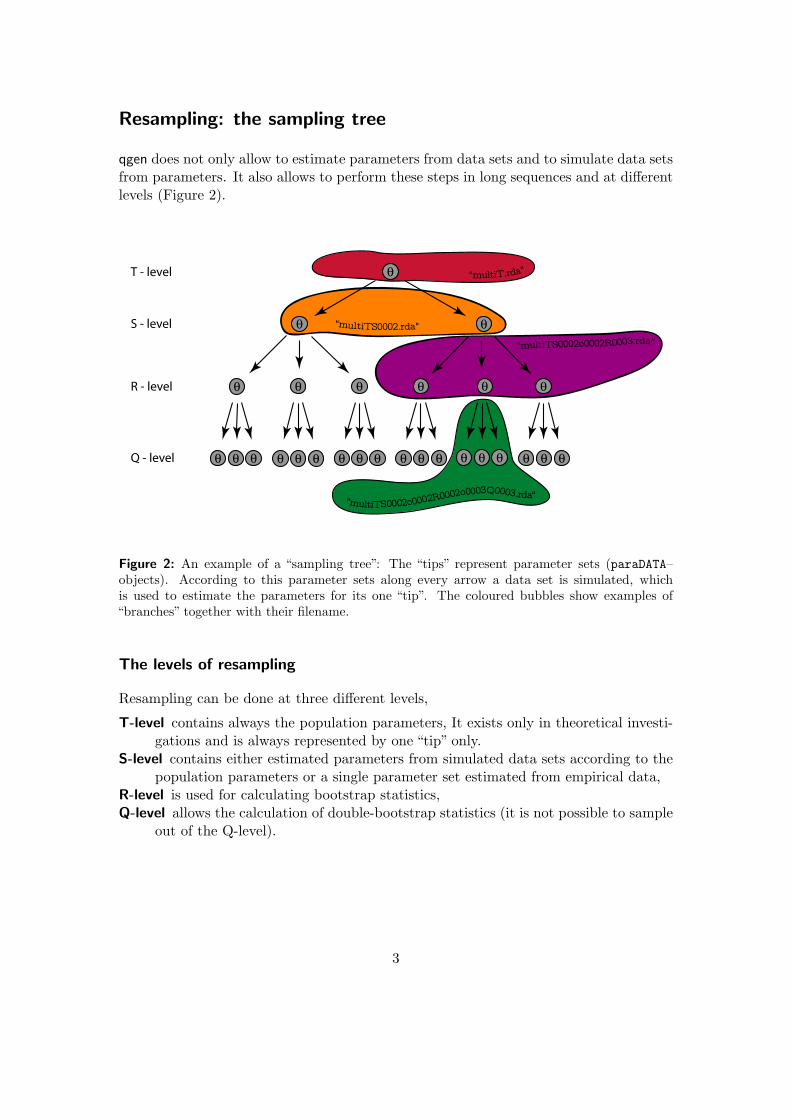
qgen does not only allow to estimate parameters from data sets and to simulate data setsfrom parameters. It also allows to perform these steps in long sequences and at differentlevels (Figure 2).
T - level
Q - level
R - level
S - level
θ
θθ
θ θ θθθθ
θθθθθθ θθθ θθθ θθθθθθ
"multiTS0002.rda"
"multiT.rda"
"multiTS0002o0002R0002o0003Q0003.rda"
"multiTS0002o0002R0003.rda"
Figure 2: An example of a “sampling tree”: The “tips” represent parameter sets (paraDATA–objects). According to this parameter sets along every arrow a data set is simulated, whichis used to estimate the parameters for its one “tip”. The coloured bubbles show examples of“branches” together with their filename.
The levels of resampling
Resampling can be done at three different levels,
T-level contains always the population parameters, It exists only in theoretical investi-gations and is always represented by one “tip” only.
S-level contains either estimated parameters from simulated data sets according to thepopulation parameters or a single parameter set estimated from empirical data,
R-level is used for calculating bootstrap statistics,Q-level allows the calculation of double-bootstrap statistics (it is not possible to sample
out of the Q-level).
3
File organisation during resampling
At every level of resampling the “sampling tree” splits up into different “branches”. Theinformation of all “tips” of a “branch” are stored within one file (summarised in a multi–object). The name of each file tells which “branch” of the “sampling tree” it contains andhow many “tips” this “branch” has. The following list describes all files created duringan investigation with qgen.
the.rda A file created by the() containing one object of class paraDATA with an emptyDATA–slot.
emp.rda A file created by emp() containing an object of class paraDATA with an emptypara–slot.
est.rda A file created by est() containing an object of class paraDATA with an emptyDATA–slot.
multiTS####.rda A file created by cal() containg an object of class multi (thefour–digit number indicates the number of “tips”, paraDATA–objects).
multiTS####o####R####.rda A file created by cal() containing an objectof class multiexample: multiTS0007o0057R0123.rda indicates that this file contains a “branch”at the“R-level”with 123 “tips”. This “branch”derived from the 7th out of 57 “tips”a the “S-level”.
multiTS####o####R####o####Q####.rda A file created by cal() con-taining an object of class multiexample: multiTS0007o0057R0001o0123Q0099.rda indicates that this file containsa “branch” at the “Q-level” with 99 tips. This “branch” derived from the first outof 123 “tips” at the “R-level” which derived from the 7th out of 57 “tips” at the“S-level”.
2 Some examples
A priory data simulation
Before you start an experiment you probably would like to know how many replicatesyou have to take to get a sufficient accurate result. By taking reasonable biological pa-rameters (additive, dominance, maternal, and environmental variance) and a samplingdesign (the number of replicates at every level, e.g, 100 sires, 6 dams each, and 3 individ-uals per dam) you can easily generate a large number of data sets. The function the()helps you to bring your assumed biological parameters into an object of class paraDATA.The sim() takes this object and samples a corresponding data set. The result is again
4

stored in an objec of class paraDATA. This object is then run by the est()–function, andafterwards by stat...()–function and you have the estimates. An example:
> stat1(est(sim(the(siN = 100, daN = 6, idN = 3, additiveVar = 100,+ dominanceVar = 100, maternalVar = 100, environmentalVar = 100))))
To repeat this step several times there are the functions, cal() and sta() to call theindividual steps in a sequence:
> parameters <- the(siN = 100, daN = 6, idN = 3, additiveVar = 100,+ dominanceVar = 100, maternalVar = 100, environmentalVar = 100,+ file = TRUE)> cal(filename = "the.rda", repetitions = 10)
A file is generated ("~/qgen/CALfile.r") that now has to be run line by line
> source("~/qgen/CALfile.r")
After some time, depending on the number of resamples, you find a file containing theesimated parameters of all 10 resampled data sets("~/qgen/multiTS0010.rda").
> sta(filename = "multiTS0010.rda", statistic.name = stat1)
The function sta() takes the multiTS0010.rda file and for every repetition the statistic(heritability for stat1()) is calculated. The results can be summarised in several ways,e.g.,
> load("/Desktop/myproject.qgen/statS.rda")> print(stat.matrix)
Analysing an empirical data set
The function emp() helps you to transform your empirical data stored in a dataframeinto an object of class paraDATA. This paraDATA–object is then analysed by the functionest() which estimates the variance components and stores them again in a paraDATA–object. The stat...() function of your choice then takes this paraDATA–object andcalculates the statistics, e.g., the stat1() calculates heritability with confidence inter-vals.
5

> data(sinapis)> a <- emp(data.use = sinapis[sinapis$fixedblock == "fb1" & sinapis$environment ==+ "contr", ], fixedblock.use = "fixedblock", character.use = "leafarea",+ environment.use = "environment", sire.use = "sire", dam.use = "dam",+ individual.use = "individual")> b <- est(a)> c <- stat1(b)> print(c)
and you receive the estimate for heritability and its confidence intervals.
Bootstrap estimates
The function emp() helps you to transform your empirical data stored in a dataframeinto an object of class paraDATA. This paraDATA–object is then analysed by the functionest() which estimates the variance components and stores them again in a paraDATA–object. The stat...() function of your choice then takes this paraDATA–object andcalculates the statistics, e.g., the stat1() calculates heritability with confidence inter-vals.
> data(sinapis)> a <- emp(data.use = sinapis[sinapis$fixedblock == "fb1" & sinapis$environment ==+ "contr", ], fixedblock.use = "fixedblock", character.use = "leafarea",+ environment.use = "environment", sire.use = "sire", dam.use = "dam",+ individual.use = "individual")> b <- est(a, file = TRUE)> cal(filename = "est.rda", repetitions = 5)> source("~/qgen/CALfile.r")> sta(filename = "multiTS0001.rda", statistic.name = stat1)> sta(filename = "multiTS0001o0001R0005.rda", statistic.name = stat1)
If you select a reasonable number of repetitions (at lest 100!) you can now calculate thebootstrap confidence intervals:
> dis()
and you receive the estimate for heritability and bootstrap confidence intervals (per-centile, Basic, BCa).
3 Outlook
The functions of qgen constrain their range of application in several ways. The followinglist describes, how some of this constraints can be relaxed.
6

> 9999 resamples The filenames reserve only four digits for numbering the differentsamples. By changing the internal function leading() this behaviour can easilybe changed simultaneously for all functions. Care has to be taken to ensure thatthe filenames do not become to long (depending on your OS)!
non–parametric resampling To save storage resources, only the estimated parametersare stored and the data sets are discharged. To change this behaviour, the functionest.R() has to be changed.
7