Exact Penalization of Generalized Nash Equilibrium Problems∗

Qin Ba Jong-Shi Pang

Original November 18, 2018

Abstract

This paper presents an exact penalization theory of the generalized Nash equilibrium problem(GNEP) that has its origin from the renowned Arrow-Debreu general economic equilibriummodel. While the latter model is the foundation of much of mathematical economics, the GNEPprovides a mathematical model of multi-agent non-cooperative competition that has found manycontemporary applications in diverse engineering domains. The most salient feature of theGNEP that distinguishes it from a standard non-cooperative (Nash) game is that each player’soptimization problem contains constraints that couple all players’ decision variables. Extendingresults for stand-alone optimization problems, the penalization theory aims to convert the GNEPinto a game of the standard kind without the coupled constraints, which is known to be morereadily amenable to solution methods and analysis. Starting with an illustrative example tomotivate the development, the paper focuses on two kinds of coupled constraints, shared (i.e.,common) and finitely representable. Constraint residual functions and the associated errorbound theory play an important role throughout the development.

1 Introduction

The Generalized Nash Equilibrium Problem (GNEP) extends the classical Nash Equilibrium Prob-lem (NEP) by allowing individual players’ constraints, in addition to the payoff functions, to dependon rival players’ strategies. This extension adds considerably descriptive and explanatory power forthe GNEP to model non-cooperative competition among multiple selfish decision-making agents.Since its introduction in the 1950’s [13, 1] (where the terms social equilibrium and abstract economywere used), the GNEP has risen beyond its mathematical-economic origin and become a commonparadigm for various engineering disciplines. This model fits well in a non-cooperative game settingwhere all players share some common resources or limitations. Thus some of the players’ constraintsare coupled ; these are in addition to the players’ private constraints that do not contain the rivalplayers’ decision variables. Sources of the GNEP include infrastructure systems such as communi-cation or radio systems [49, 50], power grids [57, 35], transportation networks [5], modern trafficsystems with e-hailing services [4], supply and demand constraints for transportation systems [54],and pollution quota for environmental application [40, 7]. We refer the readers to [22, 27, 30] formore detailed surveys on this active research topic and its many applications. The four chaptersby Facchinei published in [12, pages 151–188] contain a historical account of the GNEP, providemany references, and summarize the advances up to the year 2012.

∗Both authors are affiliated with the Daniel J. Epstein Department of Industrial and Systems Engineering, Univer-sity of Southern California, Los Angeles, California 90089-0193, U.S.A. Emails: qba@usc.edu, jongship@usc.edu.

This work was based on research supported by the National Science Foundation under grant IIS-1632971 and by theAir Force Office of Scientific Research under Grant Number FA9550-18-1-0382.

1

arX

iv:1

811.

1067

4v2

[cs

.GT

] 1

Dec

201

8

Due to the presence of the coupling constraints, solving a GNEP is a significantly more challengingtask than solving a NEP. Depending on the types of the coupling constraints, a GNEP can bedivided into two categories. The first category is the shared-constrained case, where the couplingconstraints are common to all players. [In the literature, this case has also been called jointlyconstrained, or common constrained; we adopt the “shared-constrained” terminology in this paper.]Many engineering problems cited in last paragraph are of this type. The second type is more generalin which the coupling constraints can be specific to each player and different among the players. Dueto the relative simplicity and direct connections to many engineering problems, shared-constrainedGNEPs receive most of the attention in the literature. Particularly, much effort has been spenton obtaining a special kind of equilibrium solutions, called variational equilibrium, under varioussettings and assumptions. Such an equilibrium has its origin from [52]; the term “variationalequilibrium” was coined in [22] and further explored in many papers that include [21, 27, 22, 42]where additional references can be found. In turn, the adjective “variational” was employed toexpress that this kind of equilibria of a GNEP can be described as solutions of a variationalinequality [34, 25] obtained by concatenating the first-order conditions of the players’ optimizationproblems. Alternatively, a Nikaido-Isoda-type bi-function [46] has been used extensively [41, 39, 56]as an attempt to formulate a GNEP as a single optimization problem. In general, the existence ofa variational equilibrium often relies on the convexity and certain boundedness assumptions andsuitable constraint qualifications [27]. While computationally simpler and providing a special kindof solutions, a variational equilibrium does not always have a clear advantage over a non-variationalequilibrium solution. It is hence difficult to argue that special focus should be placed on finding sucha particular equilibrium. Nevertheless, computing a non-variational equilibrium solution is morecomplex and less understood. Yet there has been some literature on this subject. For example,an extension of the class of variational equilibria is studied in [31, 44], and algorithms aiming atobtaining the entire set of solutions of special class of GNEPs are considered in [28, 19, 3]. Thepaper [53] discusses the numerical solution of an affine GNEP by Lemke’s method with an attemptto compute generalizations of variational equilibria.

With the goal of exploiting the advances in the NEPs, this paper revisits and sharpens an exactpenalization theory for GNEPs whereby the coupled constraints, shared or otherwise, are movedfrom the constraints to the objective functions via constraint residual functions scaled by a penaltyparameter. Dating back to the beginning of nonlinear programming [29], exact penalization foroptimization has been a subject of intensive study in the early days of optimization (see [33]) andmuch research has been undertaken by the Italian School led by Di Pillo, Facchinei and Grippo[14, 15, 16, 17, 18]. Exemplified by these works and references therein, this theory deals largely withproblems whose constraints are defined by differentiable inequalities and relies on the multipliers ofthese constraints. The papers [9, 8] discuss how penalty functions can be used to design numericalmethods for solving nonlinear programs that have been implemented in the very successful knitrosoftware [10]. For the GNEP, exact penalty results are derived in [26, 24] which also discuss algo-rithmic design. The paper [23] discusses extensive computational rules for updating the penaltyparameter and reports numerical results with the resulting algorithms. Contrary to exact penaliza-tion, inexact, or asymptotic penalization also penalizes the constraints but the penalty parameteris required to tend to infinity to recover a solution of the given problem. A fairly simple iterativeinexact-penalty based method for solving the GNEP was discussed in [48]; this method cast thegame as a quasi variational inequality obtained by concatenating the first-order optimality condi-tions of the players’ nonlinear programs. The recent papers [36, 37] expanded the latter paper anddiscussed augmented Lagrangian and exact penalty methods for the GNEP and the more generalquasi-variational inequality, respectively.

2

In contrast to the multiplier-based exact penalization, the principle of exact penalization, firstestablished in [11, Proposition 2.4.3] and subsequently generalized in [25, Theorem 6.8.1] dealswith the exact penalization of an abstract constraint set. The latter result makes it clear that thistheory is closely connected to the theory of error bounds [6, 43] and [25, Chapter 6]. To date,this approach has not been applied to the GNEP; part of the goal of this paper is to establish howexact penalty results for the GNEP can be derived based on an error-bound theory. Unlike a stand-alone optimization problem, a GNEP has multiple inter-connected optimization problems each withan objective function of its own; thus while exact penalty results for the players’ optimizationproblems are available, simply putting them together does not readily yield an exact penalty resultfor a GNEP. The inter-connection between the players’ optimization problems will need to beaccounted for when the coupling constraints are penalized. Furthermore, while most literatureon the exact penalization of the GNEP considers only coupling inequality constraints, see e.g.,[23, 24, 31, 36]; another goal of this paper is to bring inequality coupling constraints to the study ofexact penalization. By means of an illustrative example, we show that care is needed in choosingthe constraint residual functions in order for the conversion to a penalized NEP to be valid. Thisexample also paves the way for the theory to be developed subsequently. It is worth noting that the`q residual functions for q ∈ (1,∞) present certain advantages in guaranteeing exact penalizationof GNEP. This class of residual functions is used in [24] and [12, Chapter 3 Section 4.1]. This paperalso takes advantage of them in finitely representable cases; Sections 4 and 5 therein elucidate theadvantageous functional properties of `q residual functions in exact penalization.

2 Preliminary Discussion and Review

In this section, we present the setting of this paper and fix the notations to be used throughout.We begin with the definition of the GNEP, then review some relevant concepts and the principle ofexact penalization for an optimization problem, and finally end with an illustration of this principleapplied to a simple GNEP and a preliminary result.

2.1 The GNEP

Formally, a GNEP consists of N selfish players each of whom decides a strategy with the goalto minimize (or maximize) his/her cost (or payoff). Let xν ∈ Rnν denote the decision of playerν ∈ [N ] , 1, · · · , N. Anticipating the rival players’ strategies x−ν , (xν

′)ν ′ 6=ν , player ν ∈ [N ]

solves the following minimization problem in his/her own variable xν :

minimizexν∈C ν

θν(xν , x−ν)

subjectto xν ∈ Xν(x−ν),(1)

where θν(xν , x−ν) denotes the cost function of player ν as a function of the pair (xν , x−ν); theconstraints are of two types: those described by the private strategy set C ν ⊆ Rnν and the othersdescribed by the coupled constraint set Xν(x−ν) ⊆ Rnν that depends on the rival players’ strategytuple x−ν . [Writing (xν , x−ν) in the argument of θν(•) is to emphasize player ν’s strategy xν and

does not mean that the tuple x , (xν)Nν=1 ∈ Rn, where n ,∑ν∈[N ]

nν , is reordered such that xν is the

first block.] This setup clearly indicates that both the objective function and constraint set of eachplayer’s optimization problem are coupled by all players’ strategies. Let θ(x) , (θν(xν , x−ν))Nν=1

be the concatenation of the players’ objective functions; C ,∏ν∈[N ]

C ν be the concatenation of the

3

players’ private constraints, and X : Rn → Rn with X(x) ,∏ν∈[N ]

Xν(x−ν) be the multifunction

concatenating the players’ coupled constraints. We use the triplet (C,X; θ) to denote the GNEPwith players’ optimization problems defined by (1). A tuple x∗ , (x∗,ν)ν∈[N ] is a Nash Equilibrium(NE) of this game if x∗,ν ∈ argmin

xν∈C ν ∩Xν(x∗,−ν)

θ(xν , x∗,−ν) for all ν ∈ [N ].

By considering Xν as a multifunction from Rn−ν into Rnν , where n−ν , n − nν , the constraintxν ∈ Xν(x−ν) is equivalent to the membership that (xν , x−ν) belongs to the graph of Xν , which isdenoted by graph(Xν) ⊆ Rn. An important special case of the GNEP (C,X; θ) is when these graphsare all equal to a common set D ⊆ Rn. This is the case of common coupled constraints, whichwe call shared constraints. We denote this special case by the triplet (C,D; θ). If each functionθν(•, x−ν) is differentiable and convex and the set C ∩D is convex, then a special kind of NE of theGNEP (C,D; θ) is that derived from the variational inequality, denoted by VI (C∩D; Θ), of findinga vector x ∈ C ∩D such that (y − x)TΘ(x) ≥ 0 for all y ∈ C ∩D, where Θ(x) , (∇xνθν(x))ν∈[N ].Such a special NE is a called a variational equilibrium. When the graphs graph(Xν) are not thesame, NEs of the GNEP (C,X; θ) are related to solutions of a quasi-variational inequality; see e.g.[48] for details.

Another important special case of the GNEP (C,X; θ) is when each set Xν(x−ν) is finitely repre-sentable, i.e., when

Xν(x−ν) ,xν ∈ Rnν | g ν(xν , x−ν) ≤ 0 and hν(xν , x−ν) = 0

(2)

for some functions (g ν , h ν) : Rn → Rmν+pν with some positive integers mν and pν . Typically, suchconstraint functions g ν and hν are such that gν(•, x−ν) is differentiable and each of its componentfunctions g νi (•, x−ν) is convex and hν(•, xν) is affine; in this case, the set Xν(x−ν) is both closedand convex; see Section 5.

A road map. For the GNEP (C,X; θ) and its special cases, exact penalization aims to convertthese games with coupled constraints to standard games whereby the constraint set Xν(x−ν) foreach player is moved to the objective function via a residual function (see definition in the nextsubsection) scaled by a penalty parameter ρ, thereby obtaining a NEP (C; θρ) for a concatenatedpenalized objective θρ, whose solution is a solution of the given GNEP. Notice that we retain theprivate constraints described by the set C ν in each player’s optimization problem. Thus this isa type of partial exact penalization [24]. The development in the rest of this paper is as follows.We first present an illustrative example which reveals important insights into exact penalization ofGNEP, then consider the penalization of the GNEP (C,D; θ) with common coupled constraints andgeneral closed convex sets C and D with no particular structure. The latter part is concluded withthe case where D is finitely representable by convex inequalities and linear equalities. Finally, wediscuss the GNEP (C,X; θ) by penalizing the coupled constraints defined as in (2). We should notethat the literature on exact penalization of the GNEP has dealt largely with the latter problemunder constraint qualifications, such as the sequentially bounded CQ [26, 48] and the ExtendedMangasarian-Fromovitz constraint qualification (EMFCQ) [23, 24, 31, 36]. In this paper, we haveprovided results for exact penalization of GNEP under a strong descent assumption and a Lipschitzerror bound assumption for residual functions, see Proposition 3, Theorem 5 and Corollary 8, anda Slater-type condition for the coupled constraints, see Theorem 10 and 11.

4

2.2 Relevant concepts

We introduce in this subsection some relevant concepts that are used later. A function Φ : Rn → Rmis said to be Lipschitz continuous on a set S ⊆ Rn if, for some positive scalar LipΦ, the followingholds:

|Φ(x)− Φ(y) | ≤ LipΦ ‖x− y ‖2, ∀x, y ∈ S.

This is also referred to as Lipschitz continuity with constant LipΦ. In addition, Φ is said tobe Lipschitz continuous near a point x if, for some ε > 0, Φ is Lipschitz continuous in the ε-neighborhood of x. We hence say that Φ is locally Lipschitz continuous on S if it is Lipschitzcontinuous near every point in S. The directional derivative of Φ at a point x ∈ Rn in a directiond ∈ Rn is defined to be

Φ ′(x; d) , limτ↓0

Φ(x+ τd)− Φ(x)

τ(3)

if the limit exists. If the above limit exists for all d ∈ Rn, Φ is said to be directionally differentiableat x. It is clear that if Φ is Lipschitz continuous with constant LipΦ near x, then ‖Φ ′(x; d) ‖ (ifthe derivative exists) is bounded by LipΦ ‖ d ‖ for all d.

For two given closed subsets S and T of Rn, a function rS : Rn → R+ is a T -residual function of Sif for all x ∈ T , it holds that rS(x) = 0 if and only if x ∈ S, or equivalently if and only if x ∈ S ∩T .Note that this definition allows for S and T to have an empty intersection; in this case, the residualfunction rS is positive on T . Such a residual function rS(x) is said to yield a T -Lipschitz errorbound of S if there exist a constant γ > 0 such that

dist(x;S ∩ T ) ≤ γ rS(x), ∀x ∈ T,

where dist(x;Z) , minimumy∈Z

‖ y−x ‖2 is the distance function to a closed set Z under the Euclidean

norm. These definitions extend the usual concepts of a residual function and associated error boundof a set S which pertain to the case when T = Rn. In essence, we are interested in such quantitiesonly for elements in the subset T ; thus the restriction to the latter set. If S is finitely representabledefined by the m-dimensional vector function g and the p-dimensional vector function h as in (2),we define the `q residual function of S for a given q ∈ [1,∞] as

rq(x) ,

∥∥∥∥∥(g+(x)

h(x)

)∥∥∥∥∥q

, (4)

where g+(x) , max(g(x), 0) and ‖•‖q is the `q-norm of vectors. If each gi, i ∈ [m] is convex and h isaffine, then rq is convex for all 1 ≤ q ≤ ∞. Moreover, if these defining functions are differentiable,then for q ∈ (1,∞), rq(x) is differentiable at x 6∈ S. Its gradient is given as follows:

∇rq(x) =1

rq−1q (x)

∑i∈[m]

(g+i (x)

)q−1 ∇gi(x) +∑j∈[p]

|hj(x) |q−1 ( sgn hj(x) )∇hj(x)

, (5)

where sgn (•) is the sign function of a scalar defined to be 1 for positive numbers, -1 for negativenumbers, and 0 for 0. In the same case, the function rq(x) is directional differentiable at all x ∈ Sand its directional derivative is given by:

r ′q(x; d) =

∑i: gi(x)=0

[ max(∇gi(x)Td, 0) ]q +∑

j:hj(x)=0

| ∇hj(x)Td |q1/q

, (6)

5

As for q = 1, r1(x) is not differentiable but directional differentiable and its directional derivativeis given by:

r ′1(x; d) =∑

i: gi(x)>0

∇gi(x)Td+∑

i: gi(x)=0

max(∇gi(x)Td, 0 )+

∑j:hj(x)=0

| ∇hj(x)Td |+∑

j:hj(x)6=0

( sgn hj(x) )∇hj(x)Td.(7)

2.3 Partial exact penalization

Exact penalization of GNEPs has its origin from its counterpart for solving constrained optimizationproblems. As such, we begin by considering the following general constrained optimization problem:

minimizex∈W ∩S

f(x), (8)

where W and S represent two sets of constraints with S considered more complex than W . Bypenalizing the violation of membership in S, a penalty formulation transforms (8) into the followingpenalized optimization problem:

minimizex∈W

f(x) + ρ rS(x), (9)

where ρ > 0 is a penalty parameter to be specified and rS(x) is a W -residual function of the setS. The penalization is said to be exact for (8) if there exists a positive scalar ρ such that, for allρ ≥ ρ, every global minimizer of the penalized problem is also a global minimizer of (8) and viceversa. Note: Dealing with minimizers, this definition is a classical one. In this regard, the defini-tion is computationally most meaningful when both (8) and (9) are convex programs. Otherwise,the equivalence between the minimizers is a conceptual property that offers guidance to solve con-strained problems in practical algorithms via relaxations of some constraints. Subsequently, whenwe apply this optimization theory to the GNEP, we will make some needed convexity assumptionsso that we can freely talk about minimizers.

It is important to note that the penalized problem (9) is different from the usual one as discussedin [25, Section 6.8] which is:

minimizex∈W

f(x) + ρ rS∩W (x), (10)

where rS∩W (x) is a residual function of the intersection S ∩ W in the unrestricted sense. Assuch, while the result below is similar to [25, Theorem 6.8.1], they differ in several ways: one,the penalized problems are different; two, the error bound conditions are different; and three, theresult below does not pre-assume the solvability of either (8) or (9). This is in contrast to thesolvability assumption that is needed for one inclusion of the two argmin sets in the cited theorem.For completeness, we offer a detailed proof of the result below which does not explicitly assumeconvexity of the functions involved.

Theorem 1. Consider the nonlinear program (8) with closed sets W and S and a Lipschitz con-tinuous objective function f with constant Lipf > 0 on the set W . Assume that S ∩ W 6= ∅. LetrS(x) be a W -residual function of the set S satisfying a W -Lipschitz error bound for the set S withconstant γ > 0; i.e., rS(x) ≥ γdist(x;S ∩W ) for all x ∈W . Then for all ρ > Lipf/γ,

argminx∈S∩W

f(x) = argminx∈W

f(x) + ρ rS(x).

6

Proof. In the following two-part proof, we may assume without loss of generality that both argminsets are nonempty. We first show that the left-hand argmin is a subset of the right-hand argmin.Let x be an element of argmin

x∈S∩Wf(x). Let x ∈ W be arbitrary. Let x be a vector in S ∩ W such

that ‖x− x‖2 = dist(x;S ∩W ). We have

f(x) + ρ rS(x) ≥ f(x) + ρ γ ‖x− x ‖2 by the W -Lipschitz error bound

≥ f(x)− Lipf ‖x− x ‖2 + ρ γ ‖x− x ‖2 by the Lipschitz continuity of f

≥ f(x) by the choice of ρ

≥ f(x) = f(x) + ρ rS(x) by the optimality of x.

This establishes one inclusion. For the converse, let x∗ ∈ argminx∈W

f(x) + ρ rS(x). It suffices to show

that x∗ ∈ S. Let x be a vector in S ∩ W such that ‖x∗ − x‖2 = dist(x∗;S ∩W ). We have

f(x) ≥ f(x∗) + ρ rS(x∗) by the optimality of x∗

≥ f(x∗) + ρ γ ‖x∗ − x ‖2 by the W -Lipschitz error bound

≥ f(x)− Lipf ‖x∗ − x‖2 + ρ γ ‖x∗ − x ‖2 by the Lipschitz continuity of f

≥ f(x) by the choice of ρ.

Therefore, x∗ = x, establishing the claim and the equality of the two sets of minimizers.

We will apply Theorem 1 to the GNEP (C,X; θ) by penalizing the coupled constraint set Xν(x−ν)

in each player ν’s optimization problem. Letting C −ν ,∏ν ′ 6=ν

C ν ′ and rν(•, x−ν) be a C ν-residual

function of the set Xν(x−ν) for given x−ν ∈ C −ν , we obtain the following penalized subproblemfor player ν with respect to given x−ν :

minimizexν ∈C ν

θν(xν , x−ν) + ρ rν(xν , x−ν) (11)

where ρ > 0 is a penalty parameter which we take for simplicity to be the same for all players. LetrX(x) , (rν(x))Nν=1 and θρ;X , θ + ρ rX . Then the optimization problems (11) concatenated forall ν ∈ [N ] define the game (C; θρ;X) which is clearly a NEP. We say that exact penalization holdsfor the GNEP (C,X; θ) with residual function rX if there exists a scalar ρ > 0 such that, for allρ ≥ ρ, every equilibrium solution of the NEP (C; θρ;X) is also an equilibrium solution of the GNEP(C,X; θ) and vise versa. The following example drawn from [27] illustrates this penalization.

Example 2. Consider the shared-constrained GNEP (C,D; θ) with the following specifications:N = 2; n1 = n2 = 1; θ1(x) = (x1−1)2; θ2(x) = (x2−1/2)2; C = R2, and D = x ∈ R2 |x1+x2 ≤ 0.The set of equilibria of this GNEP is (α, 1−α) | 1/2 ≤ α ≤ 1. The set of variational equilibria ofthe GNEP is a singleton containing (3/4, 1/4). With ρ > 0 as the penalty parameter, the penalizedNEP is defined by the following two univariate optimization problems:

minimizex1

(x1 − 1)2 + ρ (x1 + x2 − 1 )+ minimizex2

(x2 − 1

2

)2+ ρ (x1 + x2 − 1 )+

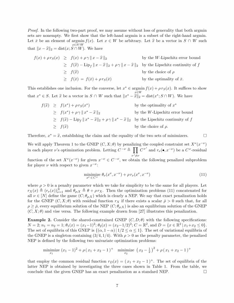
that employ the common residual function rD(x) = (x1 + x2 − 1 )+. The set of equilibria of thelatter NEP is obtained by investigating the three cases shown in Table 1. From the table, weconclude that the given GNEP has an exact penalization as a standard NEP.

7

x∗1 x∗2 equilibria set for ρ ≥ 1

x1 + x2 > 1 1− ρ/2 3/2− ρ ∅x1 + x2 < 1 1 3/2 ∅x1 + x2 = 1 [1− ρ/2, 1] [1/2− ρ/2, 1/2] (α, 1− α) | 1/2 ≤ α ≤ 1

Table 1: Three cases of the penalized problem

The primary question this paper aims at addressing is under what conditions exact penalizationholds for the GNEP (C,X; θ) and its special cases. While various exact penalization results exist forthe optimization problem (8) in the literature, stand-alone results on the GNEP are not as many;they are mostly embedded in methods for solving the game under some CQs without necessarilyclaiming the exactness of the penalization. A main difficulty in extending the penalty results for anoptimization problem to the GNEP lies in the fact that while each player’s optimization problem (1)may have an exact penalty equivalent, the penalty parameter for player ν’s problem in principledepends on the rivals’ strategy tuple x−ν ; this makes it difficult for a uniform penalty parameterto exist for all players in an NEP formulation. A related point is highlighted by the proof of theconverse inclusion in Theorem 1 which suggests that the feasibility of a solution of the penalizedNEP is key for that solution to be a solution of the original un-penalized game. This point wasmade clear in [26, Theorem 1] and the discussion that follows it where an explanation was offered.We formally state this requirement in the first part of the following preliminary result whose proofwe omit.

Proposition 3. Suppose that C and the graph of the constraint multifunction X are closed sets.Let rν(•, x−ν) be a C ν-residual function of the set Xν(x−ν), for all x−ν ∈ C −ν . The following twostatements hold:

(a) Let x∗ be a solution of the penalized NEP (C; θρ;X) for some ρ > 0. Then x∗ is a solutionof the GNEP (C,X; θ) if and only if x∗ belongs to the graph of the multifunction X; i.e.,x∗,ν ∈ Xν(x∗,−ν) for all ν ∈ [N ].

(b) Suppose that for every x−ν ∈ C −ν , C ν ∩ Xν(x−ν) 6= ∅, θν(•, x−ν) is Lipschitz continuouswith constant Lipν on the set C ν , and rν(•, x−ν) provides a C ν-Lipschitz error bound withconstant γν > 0 for the set Xν(x−ν). Then for all ρ > max

ν∈[N ]Lipν/γν , every equilibrium

solution of the penalized NEP (C; θρ;X) is an equilibrium solution of the GNEP (C,X; θ) andvice versa.

One of the main weakness of part (b) of the above proposition is the assumption that C ν ∩Xν(x−ν)is nonempty for all x−ν in C −ν . The invalidity of this assumption contributes to inequality betweenthe set of penalized NE and that of the NE of the GNEP; see parts (a) of Example 4 below.Subsequently, we will provide alternative conditions that bypass this assumption; see Theorem 5and 11.

3 An Illustrative Example

Before presenting the main results, we offer an example that summarizes several important featuresin the penalization of the shared-constrained GNEP (C,D; θ) by residual functions of the commonconstraint set D. This example provides the basis for the subsequent results that are motivated bythe various penalized NEPs discussed therein.

8

Example 4. Consider the share-constrained GNEP (C,D; θ) with the following specifications:N = 2; n1 = n2 = 1; θ1(x) = −x1; θ2(x) = −x2; C = [0, 4] × [0, 4]; D = x ∈ R2 | gi(x) ≤ 0, i =1, 2, 3; where g1(x) = x1 +x2−2, g2(x) = 2x1−x2−2, and g3 = −x1 +2x2−2. The constraint setC ∩D is shown as the gray area in Figure 1. It is easy to see that every point on the line segmentbetween (4/3, 2/3) and (2/3, 4/3) (i.e., the solid dark line segment in the figure) is a NE of thisGNEP, for which we illustrate various penalizations as follows.

x2

0 x1

g1

g2

g32

2

Figure 1: Graph illustration for Example 4

(a) `1 penalization is not exact. Using the `1 residual function r1(x) = ‖g+(x)‖1, the penalizedversion of the GNEP (C,D; θ) is the NEP (C; θ + ρ r1). While the `1 residual function is a widelyused residual function that is proven to be effective for exact penalization of many nonlinear pro-gramming problems, this example shows that it does not work generally for exact penalization ofeven shared, linearly constrained GNEPs. Specifically, we can find an equilibrium solution of thepenalized NEP (C; θ + ρ r1) but not one of the GNEP (C,D; θ). The two players’ optimizationproblems for the latter NEP are as follows:

minimize0≤x1≤4

− x1 + ρ(

[x1 + x2 − 2]+ + [2x1 − x2 − 2]+ + [−x1 + 2x2 − 2]+)

minimize0≤x2≤4

− x2 + ρ(

[x1 + x2 − 2]+ + [2x1 − x2 − 2]+ + [−x1 + 2x2 − 2]+).

By examining the different pieces of the square box C separated by the three lines in the plane, wecan conclude that, for ρ > 1, the set of equilibria of the NEP (C; θ + ρ r1) is (x1, x2) |x1 + x2 =2, 2/3 ≤ x1 ≤ 4/3 ∪ (2, 2). It is clear that (2, 2) is not an equilibrium solution of the given GNEP(C,D; θ).

This negative result is very informative; namely it suggests that unlike the case of an optimizationproblem, one needs to be selective in the penalty function in the case of the GNEP; see Theorem 5.

(b) Squared `2 penalization is not exact. The penalized problem with the squared quadraticresidual function r2

2(x) = ‖g+(x)‖22 is the NEP (C; θ+ ρ r22). It is easy to verify that for any ρ > 0,

every point in x ∈ C | g1(x) = 1/(2ρ), g2(x) ≤ 0, g3(x) ≤ 0 (i.e., the red line segment in Figure 1)is an equilibrium solution of this penalized NEP. Even though as ρ gets to infinity, these pointsconverge to equilibria of the original GNEP, for any finite ρ they do not belong to C ∩D, and thusare not equilibria of the original GNEP.

9

(c) `2 penalization is exact. The penalized problem with the `2 residual function is the NEP(C; θ + ρ r2). By (5), at x 6∈ D, the gradient of r2(x) is:

∇r2(x) =1

r2(x)

(g+

1 (x) + 2g+2 (x)− g+

3 (x)

g+1 (x)− g+

2 (x) + 2g+3 (x)

)

For any x in the interior of C \D, one can write down the equilibrium conditions of this NEP as(−1

−1

)+ ρ∇r2(x) = 0

which can be shown to have no solution for ρ > 1. Similarly, by checking the respective optimalityconditions of the two players’ optimization problems, one can conclude that any point on theboundary of C \D is not be an equilibrium solution of the NEP (C; θ+ ρ r2) either. Furthermore,by part (a) of Proposition 3, it is straightforward to see that any point of C ∩ D that is not anequilibrium solution of the GNEP (C,D; θ) cannot be one of the NEP (C; θ + ρ r2). The set ofremaining feasible points of NEP (C; θ + ρ r2) is the equilibria set of the GNEP (C,D; θ), i.e.,(x1, x2) |x1 + x2 = 2, 2/3 ≤ x1 ≤ 4/3. Using the directional derivative formula given in (6), itis possible to verify that every point in this set is an equilibrium solution of the penalized NEP(C; θ + ρ r2).

(d) `1 penalization is exact for variational equilibria. In this example, every equilibriumsolution of the GNEP (C,D; θ) is a variational equilibrium and hence a solution to the VI (C∩D; Θ).By penalizing the constraint set D of this VI using the `1 residual function (same as part (a)), weobtain the mutivalued VI (C; Θ + ρ ∂r1), where ∂ denotes the subdifferential of a convex functionas in convex analysis. It is not difficult to see that the solution set of the penalized VI agrees withthe solution set of VI (C ∩D; Θ), and hence with the equilibrium set of the GNEP (C,D; θ), forall ρ ≥ 1. This conclusion should be contrasted with part (a) where the penalization of this GNEPis via the NEP there. In terms of it first-order conditions, the latter NEP is equivalent to the

multivalued VI (C; Θ + ρR), where R is the multifunction R(x) =

3∏i=1

∂xir1(x) which is a superset

of ∂r1(x). Thus it is not unexpected that the NEP may have more solutions than the given GNEP,as confirmed by part (a).

(e) `1 penalization is exact when C is restricted. As a result of the failed exact penalizationof the GNEP (C,D; θ) in terms of the NEP (C; θ+ ρ r1) demonstrated in part (a), one could raisethe question of whether the given GNEP may be equivalent to a NEP (C, θ + ρ r1) for a certainCartesian subset C of C. It turns out that this question has an affirmative answer for this example.Indeed, a natural way to define this restricted set is C = C1 × C2 with

C1 , x1 ∈ C1 | ∃x2 ∈ C2 such that (x1, x2) ∈ D

and similarly for C2. For this example, we have C1 = C2 = [0, 4/3]. We leave it for the reader toverify that

set of equilibrium solutions of the NEP (C; θ + ρ r1)

= set of equilibrium solutions of the GNEP (C,D; θ)

= set of equilibrium solutions of the GNEP (C,D; θ).

10

The equality between the first and second set illustrates part (a) of Proposition 3. It is possible toextend the above observation to more general cases. The formal study on this is to be pursued inthe future.

An important difference between the `1 and `2 penalization is that the residual function in thelatter case is differentiable at points outside the shared constraint set D whereas that in the formeris not. This observation motivates the following consideration about the choice of the residualfunction rD. Namely, including the distance function to the set D when the latter is closed andconvex, the residual function rD needs to be at the minimum directionally differentiable. However,this alone is not enough as illustrated by part (a) in the above example. Thus a suitable conditionon the directional derivatives outside the set D is needed; such a requirement is made explicit inTheorem 5 in the next section.

4 Main Results for the GNEP (C,D; θ)

Due to the common shared constraint set D, we employ a common residual function that applies toall players’ individual optimization problems; see Examples 2 and 4 for such a function. Specifically,throughout this section, we let rD : Rn → R+ be a C-residual function of the shared constrainedset D; i.e., for all x ∈ C, rD(x) = 0 if and only if x ∈ D. It then follows that for each x−ν ∈ C− ν ,rD(•, x−ν) is a C ν-residual function of the set D ν(x−ν) , yν | (yν , x−ν) ∈ D. Conversely, wecan construct such an (aggregate) residual function rD from the latter sets D ν(x−ν). Indeed, foreach ν ∈ [N ], let rν : Rn → R+ be such that for each x−ν ∈ C− ν , rν(•, x−ν) is a C ν-residual

function of the set D ν(x−ν). It is then easy to verify that with rD(x) ,∑ν∈[N ]

rν(xν , x−ν), it holds

that for all x ∈ C, rD(x) = 0 if and only if x ∈ D. According to part (a) of Proposition 3, a keyrequirement for a solution of the penalized NEP (C; θ + ρ rD), where θ + ρ rD is a shorthand forthe vector function (θν + ρ rD)ν∈[N ], to be a solution of the GNEP (C,D; θ) is the membershipof the candidate solution on hand in the shared constraint set D. Moreover, as mentioned above,the directional differentiability of the residual function rD needs to be strengthened. Taking intoaccount these two considerations and adapting a key quantity introduced in [14], we present thefollowing Strong Descent Assumption on residual functions. It would be shown to play a vital rolein guaranteeing exact penalization of a GNEP. For a set S ⊆ Rn and a vector x ∈ S, let T (x;S)

denote the tangent cone at x to S, i.e., the collection of vectors d ∈ Rn such that d = limk→∞

xk − xτk

for some vector sequence xk ⊂ S converging to x and some positive scalar sequence τk withτk ↓ 0.

Strong Descent Assumption. Let S and W be two closed sets and rS be a W -residual functionof S. There exists a constant α > 0 such that for every x ∈ W \ S, r ′S(x; d) ≤ −α‖d‖2 for somenonzero d ∈ T (x;W ).

The above assumption appears in [14, Theorem 3.2] in the context of a single optimization problem.While it will be discussed in some more detail momentarily, the assumption essentially requiresthat a strong descent direction of the residual function exists at every infeasible point x ∈ W \ S.Considering the optimization problem (8) with Lipschitz continuous function f(x), the strongdescent assumption would disqualify every point in W \ S as a minimizer of (9) for sufficientlylarge ρ. Specialized to each player ν’s optimization problem and to the associated residual functionrD(•, x−ν), this argument leads to the next result on the exact penalization of the GNEP (C,D; θ),where convexity of the sets C, D and the functions θν(•, x−ν) is not needed.

11

Theorem 5. Suppose that C, D are closed subsets of Rn. Assume that each θν(•, x−ν) is di-rectionally differentiable and locally Lipschitz continuous with constant Lipθ > 0 on C ν for allx−ν ∈ C −ν . Let rD be a directionally differentiable C-residual function of D. If there exist positiveconstants α and α ′ such that for every x ∈ C \D, either one of the following holds:

(a) for some ν ∈ [N ] and nonzero d ν ∈ T (xν ;C ν) ⊆ Rnν ,

rD(•, x−ν) ′(xν ; d ν) ≤ −α ′ ‖ d ν ‖2 (12)

(b) for some nonzero d ∈ T (x;C),∑ν∈[N ]

rD(•, x−ν) ′(xν ; d ν) ≤ r ′D(x; d) ≤ −α ‖ d ‖2, (13)

then there exists a finite number ρ such that for every ρ > ρ, every equilibrium solution of the NEP(C; θ + ρrD) is an equilibrium solution of the GNEP (C,D; θ).

Proof. Since ‖ d ‖2 ≥1√N

∑ν∈[N ]

‖ d ν ‖2, it follows that if (b) holds for some α, then (a) holds with

α ′ = α/√N . Hence it suffices to prove the theorem under condition (a). Let x be an equilibrium

solution of the NEP (C; θ + ρ rD). By part (a) of Proposition 3, it suffices to show that x ∈ D.Assume for contradiction that x ∈ C \D. By assumption, there exist ν ∈ [N ] and d ν ∈ T (xν ;C ν)such that

rD(•, x−ν) ′(xν ; d ν) ≤ −α ′ ‖ d ν ‖2.

By the optimality of xν to player ν’s optimization problem in the NEP (C; θ + ρ rD), we have

θν(•, x−ν)′(xν ; d ν) + ρ rD(•, x−ν)′(xν ; d ν) ≥ 0

By the Lipschitz continuity of θν(•, x−ν) with constant Lipθ, we obtain

| θν(•, x−ν)′(xν ; d ν) | ≤ Lipθ ‖ d ν ‖2.

Hence, It follows thatLipθ ‖ d ν ‖2 − ρα ′ ‖ dν ‖2 ≥ 0.

By choosing of ρ =, Lipθ/α′, the above inequality yields a contradiction.

Theorem 5 is a game-theoretic extension of Theorem 1 which pertains to a single optimizationproblem. It is useful to note that the assumption of a Lipschitz error bound on the residualfunction required in the former theorem is replaced by the strong descent assumptions in thepresent game result. Furthermore, in contrary to part (b) of Proposition 3, Theorem 5 does notrequire C ν ∩ D ν(x−ν) to be nonempty for all x−ν ∈ C−ν . As shown in Example 4, the laternonemptiness condition may be too restrictive even for a simple linearly constrained GNEP. Wealso note that part (a) of Theorem 5 can be extended in a straightforward way to the general caseof GNEP (C,X; θ). The assumptions required there would involve the strong descent assumptionof rν(•, x−ν). While this result is not explicitly stated in the paper, another sufficient conditionwould be provided for the GNEP (C,X; θ) in the case that Xν(•) is finitely representable, seeTheorem 11.

In the remaining of this section, due to the relatively simpler condition, we will focus on refiningpart (b) of Theorem 5 by providing some sufficient conditions for (13) to hold. The inequality

12

on the left side of (13) is the sum property on the total directional derivative r ′D(x; y − x) withregard to the partial directional derivatives rD(•, x−ν)′(xν ; y ν − xν) for ν ∈ [N ]. The study of thisrelationship for a general function is originated from [2] (see also [55]). It is clear that when rD isconvex, this inequality is equivalent to equality as the directional derivative of a convex function issubadditive in the direction. Sufficient conditions for the equality include Gateaux differentiability,and a certain strong property of the directional derivatives that can be found in [51]. In particular,if the residual function rD is differentiable on C \D (to be precise, differentiable on a set Ω \ D,where Ω is a open set containing the set C), then the left side inequality in (13) holds readily. Thisdifferentiability assumption will be in place in the rest of the section.

The inequality on the right side of (13) is related to the inequality (15) imposed in Theorem 3.2in [14] that is for the total penalization of a single optimization problem. The cited theorem dealtwith the optimization problem minimize

x∈Dθ(x) where D is a subset of Rn and assumed in essence

to satisfy the property that there exist positive scalars α and ε such that for all x ∈ Dε \D, somey ∈ Rn \ x exists satisfying r ′D(x; y − x) ≤ −α ‖ y − x ‖, where Dε is an ε-enlargement of theset D; there was no second set C involved. For partial penalization, the incorporation of the setC in the strong descent assumption appears to be new. While this restriction reduces the set ofpotential descent directions from Rn to T (x;C), it also excludes certain infeasible points underconsideration, thus facilitating the exact penalization. We will provide a more detailed discussionon this point in subsequent subsections.

4.1 Linear metric regularity

The literature on Lipschitz error bounds for closed convex sets is vast. Summarizing previouspapers that include [47, 43, 38] and many others, Chapter 6 in the monograph [25] provides agood reference for this theory and its applications. Closely related to Lipschitz error bounds is thetheory of linear metric regularity; see [6, 45]. For our purpose, we can rephrase the strong descentassumption in terms of the latter theory. Specifically, two closed convex subsets C and D of Rnwith a nonempty intersection are said to be linearly metrically regular if there exists a constantγ ′ > 0 such that

dist(x;C ∩D) ≤ γ ′ max ( dist(x;C), dist(x;D) ) , ∀x ∈ Rn.

We remark that linear metric regularity is equivalent to the existence of a constant γ1 > 0 suchthat

dist(x;C ∩D) ≤ γ1 dist(x;D), ∀x ∈ C. (14)

The above equivalence is known in the literature, e.g., see [45, Theorem 3.1]. Yet we provide aproof here for completeness. Clearly, the former implies the latter with γ1 = γ. If the latter holds,let x ∈ Rn be arbitrary and let y be the Euclidean projection of x onto C. We then have

dist(x;C ∩D) ≤ dist(x;C) + dist(y;C ∩D)

≤ dist(x;C) + γ1 dist(x;D) ≤ ( γ1 + 1 ) max ( dist(x;C), dist(x;D) ) ,

establishing the equivalence of linear metric regularity and the inequality (14). It follows from thisequivalence that if C and D are linearly metrically regular, then a C-residual function rD of the setD satisfies a C-Lipschitz error bound if there exists a constant γ > 0 such that dist(x;D) ≤ γ rD(x)for all x ∈ C, the latter condition being a usual error bound for D with reference to vectors in C.

The result below shows that linear metric regularity (or equivalently (14)) provides a sufficientcondition for the strong descent assumption to hold.

13

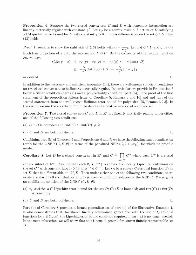
Proposition 6. Suppose the two closed convex sets C and D with nonempty intersection arelinearly metrically regular with constant γ ′. Let rD be a convex residual function of D satisfyinga C-Lipschitz error bound for D with constant γ > 0. If rD is differentiable on the set C \D, then(13) holds.

Proof. It remains to show the right side of (13) holds with α =1

γ γ ′. Let x ∈ C \D and y be the

Euclidean projection of x onto the intersection C ∩ D. By the convexity of the residual functionrD, we have

r ′D(x; y − x) ≤ rD(y)− rD(x) = −rD(x) ≤ −γ dist(x;D)

≤ − γ

γ ′dist(x;C ∩ D) = − γ

γ ′‖x− y ‖2

as desired.

In addition to the necessary and sufficient inequality (14), there are well-known sufficient conditionsfor two closed convex sets to be linearly metrically regular. In particular, we provide in Proposition 7below a Slater condition (part (a)) and a polyhedrality condition (part (b)). The proof of the firststatement of the proposition follows from [6, Corollary 5, Remark 9 and 10] and and that of thesecond statement from the well-known Hoffman error bound for polyhedra [25, Lemma 3.2.3]. Inthe result, we use the shorthand “rint” to denote the relative interior of a convex set.

Proposition 7. Two closed convex sets C and D in Rn are linearly metrically regular under eitherone of the following two conditions:

(a) C ∩D is bounded and rint(C) ∩ rint(D) 6= ∅;

(b) C and D are both polyhedra.

Combining part (b) of Theorem 5 and Propositions 6 and 7, we have the following exact penalizationresult for the GNEP (C,D; θ) in terms of the penalized NEP (C, θ + ρ rD), for which no proof isneeded.

Corollary 8. Let D be a closed convex set in Rn and C ,∏ν∈[N ]

C ν where each C ν is a closed

convex subset of Rnν . Assume that each θν(•, x−ν) is convex and locally Lipschitz continuous onthe set C ν with constant Lipθ > 0 for all x−ν ∈ C −ν . Let rD be a convex C-residual function of theset D that is differentiable on C \D. Then under either one of the following two conditions, thereexists a scalar ρ > 0 such that for all ρ > ρ, every equilibrium solution of the NEP (C; θ + ρ rD) isan equilibrium solution of the GNEP (C,D; θ):

(a) rD satisfies a C-Lipschitz error bound for the set D; C ∩D is bounded; and rint(C) ∩ rint(D)is nonempty;

(b) C and D are both polyhedra.

Part (b) of Corollary 8 provides a formal generalization of part (c) of the illustrative Example 4.It also demonstrates that, for shared linearly constrained games and with the use of `q residualfunctions for q ∈ (1,∞), the Lipschitz error bound condition required in part (a) is no longer needed.In the next subsection, we will show that this is true in general for convex finitely representable setD.

14

4.2 Shared finitely representable sets

In this subsection and the rest of the paper, we assume that the set C is compact and convex. Wediscuss the GNEP (C,D; θ) where the shared-constrained set D is finitely representable by coupleddifferentiable inequalities and linear equations. Specifically, let

D , x ∈ Rn | g(x) ≤ 0 and h(x) = 0 (15)

with h(x) = Ax − b for some matrix A ∈ Rp and vector b ∈ Rp and each gj : Rn → R for j ∈ [m]being convex and differentiable. We separate the linear and nonlinear constraints in D so thatwe can state the Slater condition more precisely; see assumption in Lemma 9. We employ the `qresidual function for an arbitrary q ∈ (1,∞) for the set D:

rq(x) ,

∥∥∥∥∥(

max( g(x), 0 )

h(x)

)∥∥∥∥∥q

, x ∈ Rn.

The function rq is continuously differentiable on the complement of the set D. Toward the for-mulation of an exact penaliztion result for the shared constrained GNEP (C,D; θ) with a finitelyrepresentable set D, we establish a consequence of the Slater CQ for the set D. This lemma isrelated to many results in the literature; but surprisingly, we cannot find a source that has thisexact result. As such, we give a detailed proof.

Lemma 9. In the above setting, let C be a compact convex set in Rn. Suppose that there existsa vector x ∈ rintC such that Ax = b and g(x) < 0. Then there exists a scalar α > 0 such that forevery x ∈ C \D, a vector x ∈ C exists such that r ′q(x; x− x) ≤ −α ‖ x− x ‖2.

Proof. Let ε > 0 be such that the closed set Bε(x) , x ∈ C | ‖x− x ‖2 ≤ ε is contained inx ∈ C | g(x) < 0 . That such a scalar ε exists is by the property of the Slater point x. Let Σ bethe family of tuples σ ∈ 0, 1,−1p such that there exists x ∈ C satisfying sgn (h(x)) = σ, wheresgn (h(x)) is the p-vector whose ith component is equal to the sign of hi(x) if hi(x) 6= 0 and equalto 0 otherwise. For each σ ∈ Σ, let

C(σ) ,

x ∈ Bε(x)

∣∣∣∣∣∣∣hi(x) = 0 if σi = 0

hi(x) > 0 if σi = 1

hi(x) < 0 if σi = 0

.

This set C(σ) must be nonempty because for any σ ∈ Σ, letting xσ be a vector in C such thatsgn (h(xσ)) = σ, by the linearlity of h and the fact that h(x) = 0, we have

sgn (h(x+ τ(xσ − x))) = sgn (h(xσ)) = σ,

thus x+ τ(xσ − x) ∈ C(σ) for all τ ∈ (0, 1] sufficiently small. Furthermore, since C is convex andx ∈ rintC, for some τ < 0 that is sufficiently close to 0, x+ τ(xσ − x) ∈ C and sgn (h(x+ τ(xσ −x))) = −σ. Therefore, Σ = −Σ and for every x ∈ C, −sgn h(x) ∈ Σ. For each σ ∈ Σ, define

µ(σ) ,

1 if σ = 0

maxx∈clC(σ)

[mini :σi 6=0

σi hi(x)

]if σ 6= 0.

15

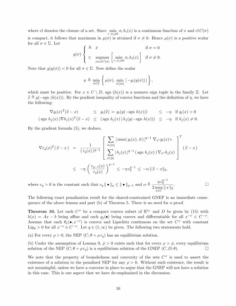
where cl denotes the closure of a set. Since mini :σi 6=0

σi hi(x) is a continuous function of x and clC(σ)

is compact, it follows that maximum in µ(σ) is attained if σ 6= 0. Hence µ(σ) is a positive scalarfor all σ ∈ Σ. Let

y(σ)

, x if σ = 0

∈ argmaxx∈clC(σ)

[mini :σi 6=0

σi hi(x)

]if σ 6= 0.

Note that g(y(σ)) < 0 for all σ ∈ Σ. Now define the scalar

η , minσ∈Σ

µ(σ), min

i∈[m][−gi(y(σ)) ]

,

which must be positive. For x ∈ C \ D, sgn (h(x)) is a nonzero sign tuple in the family Ξ. Letx , y(−sgn (h(x))). By the gradient inequality of convex functions and the definition of η, we havethe following:

∇gi(x)T(x− x) ≤ gi(x) = gi(y(−sgn h(x))) ≤ −η if gi(x) > 0

( sgn hj(x) )∇hj(x)T (x− x) ≤ ( sgn hj(x) )hj(y(−sgn h(x))) ≤ −η if hj(x) 6= 0.

By the gradient formula (5), we deduce,

∇rq(x)T ( x− x ) =1

( rq(x) )q−1

∑i∈[m]

[ max( gi(x), 0 ) ]q−1 ∇xνgi(x)+

∑j∈[p]

|hj(x) |q−1 ( sgn hj(x) )∇xνhj(x)

T

( x− x )

≤ −η(rq−1(x)

rq(x)

)q−1

≤ −η cq−1q ≤ −α ‖ x− x‖2,

where cq > 0 is the constant such that cq ‖ • ‖q ≤ ‖ • ‖q−1 and α ,η cq−1

q

2 maxx∈C‖x ‖2

.

The following exact penalization result for the shared-constrained GNEP is an immediate conse-quence of the above lemma and part (b) of Theorem 5. There is no need for a proof.

Theorem 10. Let each C ν be a compact convex subset of Rnν and D be given by (15) withh(x) = Ax − b being affine and each gj(•) being convex and differentiable for all x−ν ∈ C −ν .Assume that each θν(•, x−ν) is convex and Lipschitz continuous on the set C ν with constantLipθ > 0 for all x−ν ∈ C −ν . Let q ∈ (1,∞) be given. The following two statements hold.

(a) For every ρ > 0, the NEP (C; θ + ρ rq) has an equilibrium solution.

(b) Under the assumption of Lemma 9, ρ > 0 exists such that for every ρ > ρ, every equilibriumsolution of the NEP (C; θ + ρ rq) is a equilibrium solution of the GNEP (C,D; θ).

We note that the property of boundedness and convexity of the sets C ν is used to assert theexistence of a solution to the penalized NEP for any ρ > 0. Without such existence, the result isnot meaningful, unless we have a converse in place to argue that the GNEP will not have a solutionin this case. This is one aspect that we have de-emphasized in the discussion.

16

As a final remark of this section, we note that by following similar arguments, we can establishan exact `1-penalty result for the variational equilibria of the shared-constrained GNEP (C,D; θ)with a convex, finitely representable set D under the standard Slater condition. The proof woulduse the directional derivative formula (7) for this penalty function instead of the gradient formula(5). The details are omitted. Such a result provides a generalization of part (d) of the illustrativeExample 4.

5 Non-Shared Finitely Representable Sets

In spite of the considerable amount of literature on the exact penalization of a GNEP with coupledfinitely representable constraints, most existing results pertain to problems with only inequalityconstraints, see e.g., [23, 24, 31, 36]. The reason for the absence of such an extended treatmentto allow for equality constraints (even linear ones) is not exactly clear; one possible reason mightbe that the EMFCQ used in the aforementioned papers is not easily amenable to generalization tohandle equality constraints. In this section, we extend the discussion in Subsection 4.2 to the GNEP(C,X; θ) with non-shared coupled finitely representable constraints and show that an extendedSlater-type CQ can be imposed to yield the exact penalization for such a GNEP. Specifically, welet the sets Xν(x−ν) be defined as follows: for each x−ν ∈ C −ν ,

X ν(x−ν) ,xν ∈ Rnν | gν(xν , x−ν) ≤ 0 and hν(x) = 0

(16)

with each hν : Rn → Rpν being an affine function and each gνj : Rn → R for j ∈ [mν ] being suchthat gνj (•, x−ν) is convex and differentiable for every x−ν ∈ C −ν . We present a result that is aparallel of Theorem 10 for GNEP (C,X; θ) and then we connect the assumptions used in the resultwith the commonly used EMFCQ. Let

rν;q(x) ,

∥∥∥∥∥(

max( gν(x), 0 )

hν(x)

)∥∥∥∥∥q

, x ∈ Rn (17)

be the `q residual function for the set Xν(x−ν). This function rν;q(•, x−ν) is continuously differ-entiable on the complement of the set Xν(x−ν) for all x−ν . Let rX;q , (rν;q)ν∈[N ]. The penalized

Nash game, NEP (C; θ + ρ rX;q), consists of the following family of optimization problems:minimizexν ∈C ν

θν(xν , x−ν) + ρ rν;q(xν , x−ν)

Nν=1

,

for a given penalty parameter ρ > 0.

Theorem 11. Let each C ν be a compact convex subset of Rnν . Let each Xν be defined as in (16)with hν being affine and each gνj (•, x−ν) be convex and differentiable for all x−ν ∈ C −ν . Assumethat each θν(•, x−ν) is convex and Lipschitz continuous on the set C ν with constant Lipθ > 0 forall x−ν ∈ C −ν . Let q ∈ (1,∞) be given. The following three statements hold.

(a) For every ρ > 0, the NEP (C; θ + ρ rX;q) has an equilibrium solution.

(b) If there exists α > 0 such that for every x ∈ C not in the graph of the multifunction X, thereexists x ∈ C satisfying for some ν ∈ [N ] with xν 6∈ X ν(x−ν),

• for all i ∈ [mν ], ∇xνgνi (x ν , x−ν)T ( x ν − xν ) ≤ −α if gνi (x) > 0, and

17

• for all j ∈ [pν ],[

sgn hνj (x)]∇xνhνj (x ν , x−ν)T ( x ν − xν ) ≤ −α if hνj (x) 6= 0,

then ρ > 0 exists such that for every ρ > ρ, every equilibrium solution of the NEP (C; θ + ρ rX;q)is a equilibrium solution of the GNEP (C,X; θ).

Proof. Assertion (a) follows from a standard existence result for a NEP. In order to prove statement(b), let x∗ be an equilibrium solution of the NEP (C; θ+ρ rX;q) for some ρ > 0 which will be specifiedmomentarily. By part (a) of Proposition 3, it suffices to show that x∗ belongs to the graph of themultifunction X. Assume the contrary; let x and ν be the vector and player label, respectively,associated with x∗ as stipulated by the assumption in this part. By the gradient formula (5), wededuce,

∇xνrν;q(x∗)T ( x ν − x∗,ν )

=1

rq−1ν;q (x∗)

∑i∈[mν ]

[max( gνi (x∗), 0 )

]q−1∇xνgνi (x∗)+

∑j∈[pν ]

|hνj (x∗) |q−1 ( sgn hνj (x∗) )∇xνhνj (x∗)

T

( x ν − x∗,ν )

≤ −α(rν,q−1(x∗)

rν,q(x∗)

)q−1

≤ −α cq−1q ,

where cq > 0 is the constant such that cq ‖ • ‖q ≤ ‖ • ‖q−1. Since

x∗,ν ∈ minimizexν ∈C ν ∩X ν(x∗,−ν)

θν(xν , x∗,−ν) + ρ rν;q(xν , x∗,−ν),

we deduce0 ≤ θν(•, x∗,−ν) ′(x∗,ν ; x ν − x∗,ν) + ρ∇xνrν;q(x

∗)T ( x ν − x∗,ν )

≤ Lipθ ‖ x ν − x∗,ν ‖2 − ρα cq−1q ≤ [ Lipθ − ρ α ] ‖ x ν − x∗,ν ‖2.

where α ,α cq−1

q

2 maxx∈C‖x ‖2

. Provided that ρ > α, the above inequality yields a contradiction.

We close this paper by showing that the commonly used EMFCQ is a more restrictive assumptionthan the one imposed in part (b) of Theorem 11. Besides the fact that the EMFCQ does notadmit equality constraints, there is another subtle restriction in it; namely, included in this CQ isa condition on a feasible vector in the graph of the multifunction X, whereas the condition in part(b) of Theorem 11 does not contain such a restriction. We state the EMFCQ for a convex set C asfollows, see also [12, Definition 4.3].

(EMFCQ) This CQ is said to hold for the GNEP (C,X; θ), where each

Xν(x−ν) =xν | gν(xν , x−ν) ≤ 0

(18)

with each gνi (•, x−ν) being convex and continuously differentiable, if for every x ∈ C and ν ∈ [N ],there exists a vector x ∈ C such that

∇xνgνi (xν , x−ν)T (xν − xν) < 0 if gνi (xν , x−ν) ≥ 0.

Note that this CQ restricts even a vector x ∈ C belonging to the graph of the multifunction X,i.e., even for a feasible vector x to the GNEP. The reason to include such vectors in the CQ is so

18

that the Karush-Kuhn-Tucker conditions become valid if x turns out be an equilibrium solution ofthe GNEP. It turns out that as far as exact penalization is concerned, the validity of the CQ canbe somewhat relaxed. We have the following result.

Proposition 12. Let each C ν be a convex compact subset of Rnν and each Xν be defined as in(18) with each gνi (•, x−ν) being convex and continuously differentiable. If EMFCQ holds for theGNEP (C,X; θ) , then the assumption in part (b) of Theorem is valid.

Proof. The proof is by contradiction. We first restate the assumption in part (b) in Theorem 11 ina set-theoretic form that is more conducive to obtain the contradiction. For a given x ∈ C, let

Iν(x) ,i ∈ 1, · · · ,mν | g νi (xν , x−ν) > 0

be the index set of violated constraints in Xν(x−ν) by xν . The statement that xν 6∈ Xν(x−ν) isequivalent to Iν(x) 6= ∅. Also let

I(x) , ν ∈ [N ] | Iν(x) 6= ∅

be the player labels ν for which there is at least one constraint in Xν(x−ν) that is not satisfied byxν . Thus x 6∈ graph(X) if and only if I(x) 6= ∅. Coupled with a y ∈ C, define the quantity

αν(x, y) , maxi∈Iν(x)

∇xνg νi (xν , x−ν)T (y ν − xν).

By convention, the maximum over the empty set is equal to −∞. For a given vector x ∈ C not ingraph(X) and a player label ν ∈ I(x), the quantity αν(x, •) is a continuous function on C. Thusit is justified to define the scalar

γ , supx∈C\graph(X)

[minν∈I(x)

(miny∈C

αν(x, y)

)],

where we use sup instead of max because the latter may not be attained. Now, the assumptionin part (b) in Theorem 11 becomes γ < 0. So to prove the proposition by contradiction, supposeγ ≥ 0. Then there exist a sequence of vectors xk ⊂ C and a sequence of positive scalars εk ↓ 0such that for every k, xk 6∈ graph(X) and there exists νk ∈ I(xk) such that min

y∈Cανk(xk, y) ≥ −εk.

Without loss of generality, we may assume that the sequence xk converges to a vector x∞ ∈ C.Since there are only finitely many players, it follows that there exists a subsequence xkk∈κ anda player label ν such that for all k ∈ κ, we have ν ∈ I(xk) and min

y∈Cαν(xk, y) ≥ −εk. Hence for

all y ∈ C, αν(xk, y) ≥ −εk for all k ∈ κ. Passing to the limit k(∈ κ) → ∞, we deduce thatminy∈C

αν(x∞, y) ≥ 0. Since ν ∈ I(xk) for all k ∈ κ, it follows that g νi (x∞) ≥ 0 for all i ∈ Iν(x∞).

Thus we have obtained the following

∀ y ∈ C ∃ i such that g νi (x∞) ≥ 0 and ∇xνg νi (x∞,ν , x∞,−ν)T (y ν − x∞,ν) ≥ 0.

But this contradicts the EMFCQ applied to x∞ which asserts that there exists x ∈ C such that∇xνg νi (x∞,ν , x∞,−ν)T (x ν − x∞,ν) < 0 whenever g νi (x∞,ν , x∞,−ν) ≥ 0.

Conclusion. In this paper, we have provided a comprehensive exact penalization theory for theGNEP, by putting together a systematic study of the subject that begins with an illustrativeexample and ends with a pair of results for the cases of finitely representable constraint sets. In the

19

process, we have clarified the role of error bounds and constraint qualifications in the developedtheory; this is something that has not been sufficiently emphasized in the existing literature of theGNEP. How these exact penalization results can be put to use in the development of improvedalgorithms for computing an equilibrium solution of the GNEP remains to be investigated.

Acknowledgement. The authors are grateful to Christian Kanzow and Francisco Facchinei forsome helpful comments on a draft of this paper.

References

[1] Kenneth J. Arrow and Gerard Debreu. Existence of an equilibrium for a competitive economy.Econometrica: Journal of the Econometric Society 22(3): 265–290, 1954.

[2] Alfred Auslender. Optimisation Methodes Numeriques. Masson, Paris, France, 1976.

[3] Didier Aussel and Simone Sagratella Sufficient conditions to compute any solution of aquasivariational inequality via a variational inequality. Mathematical Methods of OperationsResearch 85(1), 3–18, 2017.

[4] Jeff X. Ban, Jong-Shi Pang, and Maged Dessouky. A general equilibrium model for trans-portation systems with e-hailing services and flow congestion. Manuscript, Department ofIndustrial and Systems Engineering, University of Southern California. September 2018.

[5] A Bassanini, A La Bella, and A Nastasi. Allocation of railroad capacity under competition:a game theoretic approach to track time pricing. In Transportation and Network Analysis:Current Trends, pages 1–17. Springer, 2002.

[6] Heinz H. Bauschke, Jonathan M. Borwein, and Wu Li. Strong conical hull intersectionproperty, bounded linear regularity, Jameson’s property (g), and error bounds in convexoptimization. Mathematical Programming 86(1):135–160, 1999.

[7] Michele Breton, Georges Zaccour, and Mehdi Zahaf. A game-theoretic formulation ofjoint implementation of environmental projects. European Journal of Operational Research168(1):221–239, 2006.

[8] Richard H. Byrd, Jorge Nocedal, and Richard A. Waltz. Steering exact penalty methods fornonlinear programming. Optimization Methods and Software 23(2): 197–213, 2008.

[9] Richard H. Byrd, G Lopez-Calva, and Jorge Nocedal. A line search exact penalty methodusing steering rules. Mathematical Programming 133(1-2): 39–73, 2012.

[10] Richard H. Byrd, Jorge Nocedal, and Richard A. Waltz. Knitro: An integrated packagefor nonlinear optimization. In G. Di Pillo and M. Roma, editors. Large-Scale NonlinearOptimization, pages 35–59, Springer, Boston, 2006.

[11] Francis H. Clarke. Optimization and Nonsmooth Analysis. Classics in Applied Mathematics,Volume 5, Society for Industrial and Applied Mathematics, 1990. [Reprint from John WileyPublishers, New York 1983.]

[12] Roberto Cominetti, Francisco Facchinei and Jean-Bernard Lasserre. Authors. Modern Opti-mization Modeling Techniques. Birkhauser Springer Basel, 2012. 10.1007/978-3-0348-0291-8.

20

[13] Gerard Debreu. A social equilibrium existence theorem. Proceedings of the National Academyof Sciences 38(10):886–893, 1952.

[14] Vladimir F. Demyanov, Gianni Di Pillo, and Francisco Facchinei. Exact penalization viaDini and Hadamard conditional derivatives. Optimization Methods and Software 9(1-3):19–36, 1998.

[15] Gianni Di Pillo and F Facchinei. Exact penalty functions for nondifferentiable programmingproblems. In Nonsmooth optimization and related topics, pages 89–107. Springer, 1989.

[16] Gianni Di Pillo and Francisco Facchinei. Regularity conditions and exact penalty functions inLipschitz programming problems. Nonsmooth optimization methods and applications, pages107–120, 1992.

[17] Gianni Di Pillo and Francisco Facchinei. Exact barrier function methods for Lipschitz pro-grams. Applied Mathematics and Optimization 32(1):1–31, 1995.

[18] G. Di Pillo and L. Grippo Exact penalty functions in constrained optimization. SIAM Journalon control and optimization 27(6), 1333–1360, 1989.

[19] Axel Dreves. Computing all solutions of linear generalized Nash equilibrium problems. Math-ematical Methods of Operations Research 85(2):207–221, 2017.

[20] Axel Dreves, Francisco Facchinei, Christian Kanzow, and Simone Sagratella. On the solu-tion of the KKT conditions of generalized Nash equilibrium problems. SIAM Journal onOptimization 21(3):1082–1108, 2011.

[21] Francisco Facchinei, Andreas Fischer, and Veronica Piccialli. On generalized Nash games andvariational inequalities. Operations Research Letters 35:159–164, 2007.

[22] Francisco Facchinei and Christian Kanzow. Generalized Nash equilibrium problems. Annalsof Operations Research 175(1):177–211, 2007.

[23] Francisco Facchinei and Christian Kanzow. Penalty methods for the solution of generalizedNash equilibrium problems. SIAM Journal on Optimization 20(5):2228–2253, 2010.

[24] Facchinei Facchinei and Lorenzo Lampariello. Partial penalization for the solution of gener-alized Nash equilibrium problems. Journal of Global Optimization 50(1): 39–50, 2011.

[25] Francisco Facchinei and Jong-Shi Pang. Finite-dimensional variational inequalities and com-plementarity problems. Springer Science & Business Media, 2003.

[26] Francisco Facchinei and Jong-Shi Pang. Exact penalty functions for generalized Nash prob-lems. In Large-scale nonlinear optimization, pages 115–126. Springer, 2006.

[27] Francisco Facchinei and Jong-Shi Pang. Nash equilibria: the variational approach. Chapter 12in Daniel P. Palomar and Yonica C. Eldar, editors. Convex optimization in signal processingand communications, Cambridge University Press, pages 443–493, 2010.

[28] Francisco Facchinei and Simone Sagratella. On the computation of all solutions of jointlyconvex generalized Nash equilibrium problems. Optimization Letters, 5(3):531–547, 2011.

21

[29] Anthony V. Fiacco and Garth P. McCormick. Nonlinear Programming: Sequential Uncon-strained Minimization Techniques. Classics in Applied Mathematics, Volume 4, Society forIndustrial and Applied Mathematics, 1990. [Reprint from John Wiley Publishers, New York1968.]

[30] Andreas Fischer, Markus Herrich, and Klaus Schonefeld. Generalized Nash equilibriumproblems-recent advances and challenges. Pesquisa Operacional, 34(3):521–558, 2014.

[31] Masao Fukushima. Restricted generalized Nash equilibria and controlled penalty algorithm.Computational Management Science, 8(3):201–218, 2011.

[32] J Gwinner. On the penalty method for constrained variational inequalities. Optimization:Theory and Algorithms 86(1): 197–211, 1983.

[33] S.P. Han and O.L. Mangasarian. Exact penalty functions in nonlinear programming. Math-ematical Programming 17(1): 251–269, 1979.

[34] Patrick T Harker. Generalized Nash games and quasi-variational inequalities. EuropeanJournal of Operational Research 54(1): 81–94, 1991.

[35] Benjamin F. Hobbs and Jong-Shi Pang. Nash-cournot equilibria in electric power marketswith piecewise linear demand functions and joint constraints. Operations Research 55(1):113–127, 2007.

[36] Christian Kanzow and Daniel Steck. Augmented Lagrangian and exact penalty methods forgeneralized Nash equilibrium problems. SIAM Journal on Optimization 26(4): 2034-2058.

[37] Christian Kanzow and Daniel Steck. Augmented Lagrangian and exact penalty methods forquasi-variational inequalities. Computational Optimization and Applications 69(3): 801-824,2018.

[38] Diethard Klatte and Wu Li. Asymptotic constraint qualifications and global error bounds forconvex inequalities. Mathematical Programming 84(1): 137–160, 1999.

[39] Jacek B. Krawczyk. Numerical solutions to coupled-constraint (or generalised) Nash equilib-rium problems. Computational Management Science 4(2): 183–204 2007.

[40] Jacek B. Krawczyk. Coupled constraint Nash equilibria in environmental games. Resourceand Energy Economics 27(2): 157–181, 2005.

[41] Jacek B. Krawczyk and Stanislav Uryasev. Relaxation algorithms to find Nash equilibriawith economic applications. Environmental Modeling and Assessment 5: 63-73 (2000).

[42] Ankur A. Kulkarni and Uday V. Shanbhag. On the variational equilibrium as a refinementof the generalized Nash equilibrium. Automatica 48(1) 45–55, 2012.

[43] Adrian S. Lewis and Jong-Shi Pang. Error bounds for convex inequality systems. In Gener-alized convexity, generalized monotonicity: recent results, pages 75–110. Springer, 1998.

[44] Koichi Nabetani, Paul Tseng, and Masao Fukushima. Parametrized variational inequalityapproaches to generalized Nash equilibrium problems with shared constraints. ComputationalOptimization and Applications 48(3):423–452, 2011.

22

[45] Kung Fu Ng and Wei Hong Yang. Regularities and their relations to error bounds. Mathe-matical Programming 99(3):521–538, 2004.

[46] Hukukane Nikaido and Kazuo Isoda. Note on noncooperative convex games. Pacific Journalof Mathematics 5(Suppl. 1): 807-815, 1955.

[47] Jong-Shi Pang. Error bounds in mathematical programming. Mathematical Programming79(1-3):299–332, 1997.

[48] Jong-Shi Pang and Masao Fukushima. Quasi-variational inequalities, generalized Nash equi-libria, and multi-leader-follower games. Computational Management Science 2: 21-56, 2005.[Erratum: same journal 6: 373-375, 2009.]

[49] Jong-Shi Pang, Gesualdo Scutari, Francisco Facchinei, and Chaoxiong Wang. Distributedpower allocation with rate constraints in gaussian parallel interference channels. IEEE Trans-actions on Information Theory 54(8):3471–3489, 2008.

[50] Jong-Shi Pang, Gesualdo Scutari, Daniel P. Palomar, and Francisco Facchinei. Design ofcognitive radio systems under temperature-interference constraints: A variational inequalityapproach. IEEE Transactions on Signal Processing 58(6):3251–3271, 2010.

[51] Stephen M. Robinson. An implicit-function theorem for a class of nonsmooth functions.Mathematics of Operations Research 16(2): 292–309, 1991.

[52] J. Ben Rosen. Existence and uniqueness of equilibrium points for concave n-person games.Econometrica: Journal of the Econometric Society 33(3):520–534, 1965.

[53] Dand A. Schiro, Jong-Shi Pang, and Uday V. Shanbhag. On the solution of affine general-ized Nash equilibrium problems with shared constraints by Lemke’s method. MathematicalProgramming, Series A 146(1):1–46, 2013.

[54] Oliver Stein and Nathan Sudermann-Merx. The noncooperative transportation problem andlinear generalized Nash games. European Journal of Operational Research 266(2):543–553,2018.

[55] Paul Tseng. Convergence of a block coordinate descent method for nondifferentiable mini-mization. Journal of Optimization Theory and Applications 109(3): 475–494, 2002.

[56] Anna von Heusinger and Christian Kanzow. Optimization reformulations of the generalizedNash equilibrium problem using nikaido-isoda-type functions. Computational Optimizationand Applications 43(3):353–377, 2009.

[57] Jing-Yuan Wei and Yves Smeers. Spatial oligopolistic electricity models with Cournot gen-erators and regulated transmission prices. Operations Research 47(1):102–112, 1999.

23