ENTROPY BALANCING IS DOUBLY ROBUST

QINGYUAN ZHAO

Department of Statistics, Stanford University

DANIEL PERCIVAL

Google Inc.

Abstract. Covariate balance is a conventional key diagnostic for methods

used estimating causal effects from observational studies. Recently, there is anemerging interest in directly incorporating covariate balance in the estimation.

We study a recently proposed entropy maximization method called Entropy

Balancing (EB), which exactly matches the covariate moments for the differ-ent experimental groups in its optimization problem. We show EB is doubly

robust with respect to linear outcome regression and logistic propensity score

regression, and it reaches the asymptotic semiparametric variance bound whenboth regressions are correctly specified. This is surprising to us because there

is no attempt to model the outcome or the treatment assignment in the orig-

inal proposal of EB. Our theoretical results and simulations suggest that EBis a very appealing alternative to the conventional weighting estimators that

estimate the propensity score by maximum likelihood.

1. Introduction

Consider a typical setting of observational study that two conditions (“treat-ment” and “control”) are not randomly assigned to the units. Deriving a causalconclusion from such observational data is essentially difficult because the treatmentexposure may be related to some covariates that are also related to the outcome.In this case, those covariates may be imbalanced between the treatment groups andthe naive mean causal effect estimator can be severely biased.

To adjust for the covariate imbalance, the seminal work of Rosenbaum and Ru-bin (1983) pointed out the essential role of propensity score, the probability ofexposure to treatment conditional on observed covariates. This quantity, rarelyknown in an observation study, may be estimated from the data. Based on theestimated propensity score, many statistical methods are proposed to estimate the

E-mail addresses: qyzhao@stanford.edu, dancsi@google.com.Date: March 10, 2016.Key words and phrases. Causal Inference, Double Robustness, Exponential Tilting, Convex

Optimization, Survey Sampling.We would like to thank Jens Hainmueller, Trevor Hastie, Hera He, William Heavlin, Diane

Lambert, Daryl Pregibon, James Robins, Jean Steiner and one anonymous reviewer for their very

helpful comments.

1

2 ENTROPY BALANCING

mean causal effect. The most popular approaches are matching (e.g. Rosenbaumand Rubin, 1985; Abadie and Imbens, 2006), stratification (e.g. Rosenbaum andRubin, 1984), and weighting (e.g. Robins et al., 1994; Hirano and Imbens, 2001).Theoretically, propensity score weighting is the most attractive among these meth-ods. Hirano et al. (2003) showed that nonparametric propensity score weighting canachieve the semiparametric efficiency bound for the estimation of mean causal ef-fect derived by Hahn (1998). Another desirable property is double robustness. Thepioneering work of Robins et al. (1994) pointed out that propensity score weightingcan be further augmented by an outcome regression model. The resulting estimatorhas the so-called double robustness property:

Property 1. If either the propensity score model or the outcome regression modelis correctly specified, the mean causal effect estimator is statistically consistent.

In practice, the success of any propensity score method hinges on the quality ofthe estimated propensity score. The weighting methods are usually more sensitiveto model misspecification than matching and stratification, and furthermore, thisbias can even be amplified by a doubly robust estimator, which is brought to atten-tion by Kang and Schafer (2007). In order to avoid model misspecification, appliedresearchers usually increase the complexity of the propensity score model until asufficiently balanced solution is found. This cyclical process of modeling propensityscore and checking covariate balance is criticized as the “propensity score tautol-ogy” by Imai et al. (2008) and, moreover, has no guarantee of finding a satisfactorysolution eventually.

Recently, there is an emerging interest, particularly among applied researchers,in directly incorporating covariate balance in the estimation procedure, so thereis no need to check covariate balance repeatedly (e.g. Diamond and Sekhon, 2013;Imai and Ratkovic, 2014; Zubizarreta, 2015). In this paper, we study a method ofthis kind called Entropy Balancing (hereafter EB) that is proposed by Hainmueller(2011). In a nutshell, EB solves an (convex) entropy maximization problem underthe constraint of exact balance of covariate moments. Due to its easy interpreta-tion and fast computation, EB has already gained some popularity in applied fields(Marcus, 2013; Ferwerda, 2014). However, little do we known about the theoreticalproperties of EB. The original proposal in Hainmueller (2011) did not give a con-dition such that EB is guaranteed to give a consistent estimate of the mean causaleffect.

In this paper, we shall show EB is indeed a very appealing propensity scoreweighting method. We find EB simultaneously fits a logistic regression model forthe propensity score and a linear regression model for the outcome. The linearpredictors of these regression models are the covariate moments being balanced.We shall prove EB is doubly robust (Property 1), in the sense that if at leastone of the two models are correctly specified, EB is consistent for the PopulationAverage Treatment effect for the Treated (PATT), a common quantity of interestin causal inference and survey sampling. Moreover, EB is sample bounded (Tan,2010), meaning the PATT estimator is always within the range of the observed out-comes, and it is semiparametrically efficient if both models are correctly specified.Lastly, The two linear models have an exact correspondence to the primal and dualoptimization problem used to solve EB, revealing an interesting connection betweendoubly robust estimation and convex optimization.

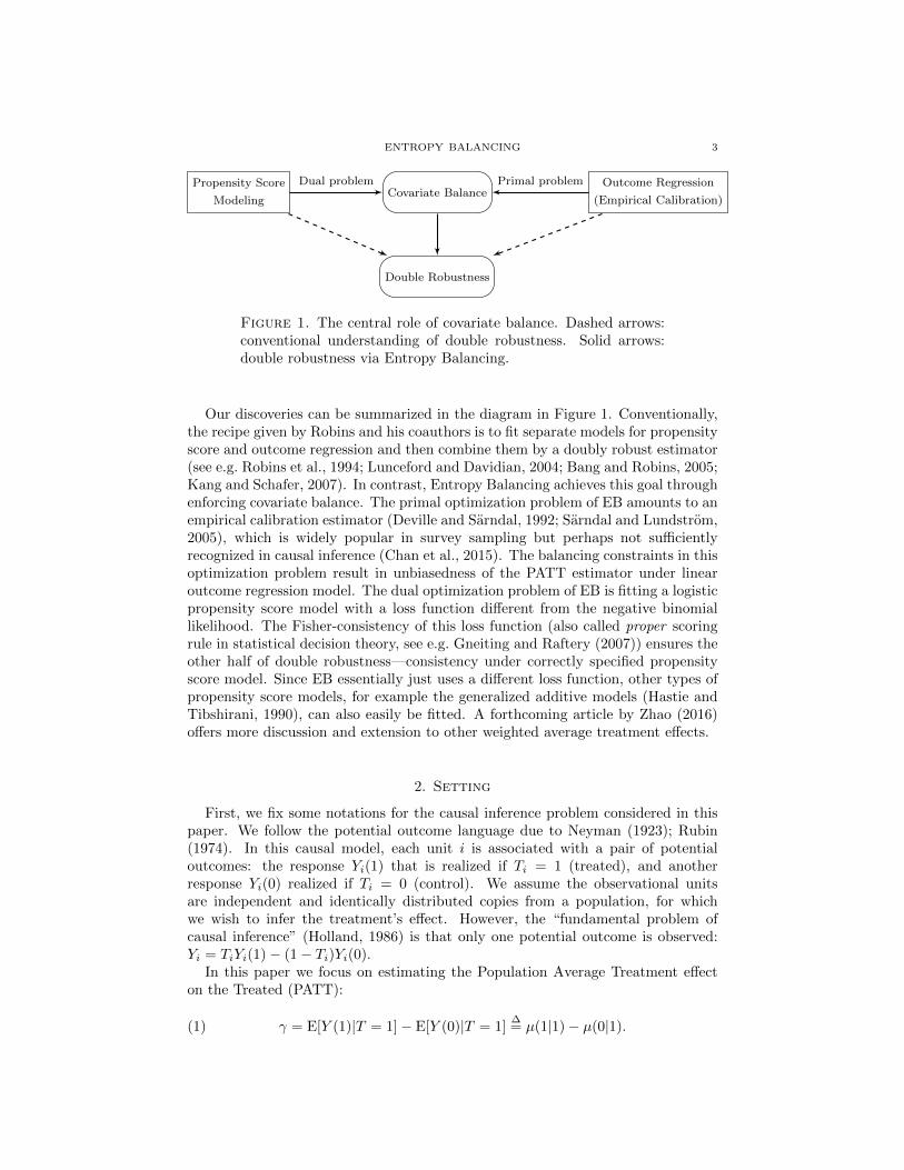
ENTROPY BALANCING 3

Propensity Score

ModelingCovariate Balance

Outcome Regression

(Empirical Calibration)

Double Robustness

Dual problem Primal problem

Figure 1. The central role of covariate balance. Dashed arrows:conventional understanding of double robustness. Solid arrows:double robustness via Entropy Balancing.

Our discoveries can be summarized in the diagram in Figure 1. Conventionally,the recipe given by Robins and his coauthors is to fit separate models for propensityscore and outcome regression and then combine them by a doubly robust estimator(see e.g. Robins et al., 1994; Lunceford and Davidian, 2004; Bang and Robins, 2005;Kang and Schafer, 2007). In contrast, Entropy Balancing achieves this goal throughenforcing covariate balance. The primal optimization problem of EB amounts to anempirical calibration estimator (Deville and Sarndal, 1992; Sarndal and Lundstrom,2005), which is widely popular in survey sampling but perhaps not sufficientlyrecognized in causal inference (Chan et al., 2015). The balancing constraints in thisoptimization problem result in unbiasedness of the PATT estimator under linearoutcome regression model. The dual optimization problem of EB is fitting a logisticpropensity score model with a loss function different from the negative binomiallikelihood. The Fisher-consistency of this loss function (also called proper scoringrule in statistical decision theory, see e.g. Gneiting and Raftery (2007)) ensures theother half of double robustness—consistency under correctly specified propensityscore model. Since EB essentially just uses a different loss function, other types ofpropensity score models, for example the generalized additive models (Hastie andTibshirani, 1990), can also easily be fitted. A forthcoming article by Zhao (2016)offers more discussion and extension to other weighted average treatment effects.

2. Setting

First, we fix some notations for the causal inference problem considered in thispaper. We follow the potential outcome language due to Neyman (1923); Rubin(1974). In this causal model, each unit i is associated with a pair of potentialoutcomes: the response Yi(1) that is realized if Ti = 1 (treated), and anotherresponse Yi(0) realized if Ti = 0 (control). We assume the observational unitsare independent and identically distributed copies from a population, for whichwe wish to infer the treatment’s effect. However, the “fundamental problem ofcausal inference” (Holland, 1986) is that only one potential outcome is observed:Yi = TiYi(1)− (1− Ti)Yi(0).

In this paper we focus on estimating the Population Average Treatment effecton the Treated (PATT):

(1) γ = E[Y (1)|T = 1]− E[Y (0)|T = 1]∆= µ(1|1)− µ(0|1).

4 ENTROPY BALANCING

The counterfactual mean µ(0|1) = E[Y (0)|T = 1] also naturally occurs in surveysampling with missing data (Deville and Sarndal, 1992; Sarndal and Lundstrom,2005) if Y (0) is the only outcome of interest and T = 1 stands for non-response.

Along with the treatment exposure Ti and outcome Yi, each experiment unit iis usually associated with a set of covariates denoted by Xi measured prior to thetreatment assignment. In a typical observational study, both treatment assignmentand outcome may be related to the covariates, which can cause serious selectionbias. The seminal work by Rosenbaum and Rubin (1983) suggested it is possibleto correct this selection bias under the following two assumptions:

Assumption 1 (strong ignorability). (Y (0), Y (1)) ⊥ T | X.

Assumption 2 (overlap). 0 < P(T = 1|X) < 1.

Intuitively, the first assumption implies that the observed covariates contain allthe information that may cause the selection bias, i.e. there is no confoundingvariable, and the second assumption ensures this bias-correction information ispresent across the entire domain of X.

Since the covariatesX contain all the information of selection bias, it is importantto understand the relationship between T, Y and X. Under Assumption 1 (strongignorability), the joint distribution of (X,Y, T ) is determined by the marginal dis-tribution of X and two conditional distributions given X. The first conditionaldistribution e(X) = P (T = 1|X) is often called the propensity score and plays acentral role in causal inference. Rosenbaum and Rubin (1983) proved that underAssumptions 1 (strong ignorability) and 2 (overlap) (Y (0), Y (1)) ⊥ T | e(X), i.e.the propensity score function e(X) itself is sufficient to produce unbiased estimatesof causal effect. The second conditional distribution is the density of Y (0) and Y (1)given X. Since we only consider the mean causal effect in this paper, it suffices tostudy the regression functions g0(X) = E[Y (0)|X] and g1(X) = E[Y (1)|X].

To estimate the PATT defined in (1), a conventional weighting estimator basedon the propensity score is the inverse probability weighting (IPW) estimator

γIPW =∑Ti=1

1

n1Yi −

∑Ti=0

e(Xi)(1− e(Xi))−1∑

Ti=0 e(Xi)(1− e(Xi))−1Yi.(2)

Here∑Ti=t

is defined as summation over all units i such that Ti = t. This notationwill be repeatedly used throughout the paper. In this formula, the control units areassociated with weights proportional to e(Xi)(1− e(Xi))

−1 to resemble the full pop-ulation. The most popular choice of obtaining e(x) is via logistic regression, wherelogit(e(x)) is modeled by

∑pj=1 θjcj(x) and cj(x) are functions of the covariates.

3. Entropy Balancing

Entropy Balancing (EB) is an alternative weighting method proposed by Hain-mueller (2011) to estimate PATT. EB operates by maximizing the entropy of the

ENTROPY BALANCING 5

weights under some pre-specified balancing constraints:

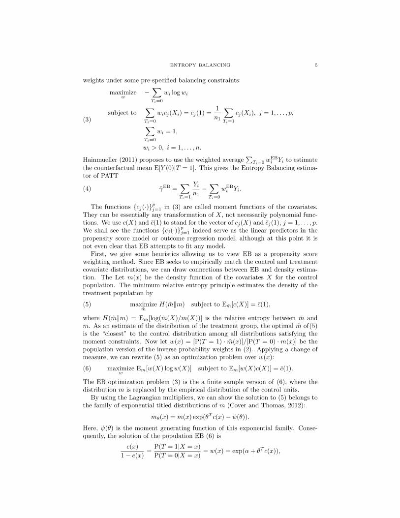
(3)

maximizew

−∑Ti=0

wi logwi

subject to∑Ti=0

wicj(Xi) = cj(1) =1

n1

∑Ti=1

cj(Xi), j = 1, . . . , p,

∑Ti=0

wi = 1,

wi > 0, i = 1, . . . , n.

Hainmueller (2011) proposes to use the weighted average∑Ti=0 w

EBi Yi to estimate

the counterfactual mean E[Y (0)|T = 1]. This gives the Entropy Balancing estima-tor of PATT

(4) γEB =∑Ti=1

Yin1−∑Ti=0

wEBi Yi.

The functions cj(·)pj=1 in (3) are called moment functions of the covariates.They can be essentially any transformation of X, not necessarily polynomial func-tions. We use c(X) and c(1) to stand for the vector of cj(X) and cj(1), j = 1, . . . , p.We shall see the functions cj(·)pj=1 indeed serve as the linear predictors in thepropensity score model or outcome regression model, although at this point it isnot even clear that EB attempts to fit any model.

First, we give some heuristics allowing us to view EB as a propensity scoreweighting method. Since EB seeks to empirically match the control and treatmentcovariate distributions, we can draw connections between EB and density estima-tion. The Let m(x) be the density function of the covariates X for the controlpopulation. The minimum relative entropy principle estimates the density of thetreatment population by

(5) maximizem

H(m‖m) subject to Em[c(X)] = c(1),

where H(m‖m) = Em[log(m(X)/m(X))] is the relative entropy between m andm. As an estimate of the distribution of the treatment group, the optimal m of(5)is the “closest” to the control distribution among all distributions satisfying themoment constraints. Now let w(x) = [P(T = 1) · m(x)]/[P(T = 0) ·m(x)] be thepopulation version of the inverse probability weights in (2). Applying a change ofmeasure, we can rewrite (5) as an optimization problem over w(x):

(6) maximizew

Em[w(X) logw(X)] subject to Em[w(X)c(X)] = c(1).

The EB optimization problem (3) is the a finite sample version of (6), where thedistribution m is replaced by the empirical distribution of the control units.

By using the Lagrangian multipliers, we can show the solution to (5) belongs tothe family of exponential titled distributions of m (Cover and Thomas, 2012):

mθ(x) = m(x) exp(θT c(x)− ψ(θ)).

Here, ψ(θ) is the moment generating function of this exponential family. Conse-quently, the solution of the population EB (6) is

e(x)

1− e(x)=

P(T = 1|X = x)

P(T = 0|X = x)= w(x) = exp(α+ θT c(x)),

6 ENTROPY BALANCING

where α = log(P(T = 1)/P(T = 0)). This is exactly the logistic regression modelof the propensity score using c(x) as predictors.

Notice that EB is different from the maximum likelihood fit of the logistic re-gression. The dual optimization problem of (3) is

(7) minimizeθ

log

∑Ti=0

exp

( p∑j=1

θjcj(Xi)

)− p∑j=1

θj cj(1),

whereas the maximum likelihood solves

(8) minimizeθ

n∑i=1

log

1 + exp

(− (2Ti − 1)

p∑j=1

θjcj(Xi)

) .

It is apparent from (7) and (8) that EB and maximum likelihood use different lossfunctions.

The optimization problem (7) can be shown to be strictly convex, and the unique

solution θEB can be quickly computed by Newton method. The EB weights (so-lution to the primal problem (3)) are given by the Karush-Kuhn-Tucker (KKT)conditions: for any i such that Ti = 0,

(9) wEBi =

exp(∑p

j=1 θEBj cj(Xi)

)∑Ti=0 exp

(∑pj=1 θ

EBj cp(Xi)

) .Entropy Balancing bridges two existing approaches of estimating the mean causal

effect

(1) The calibration estimator that is very popular in survey sampling (Devilleand Sarndal, 1992; Sarndal and Lundstrom, 2005; Chan et al., 2015);

(2) The empirical likelihood approach that significantly advances the theory ofdoubly robust estimation in observation study (Wang and Rao, 2002; Tan,2006; Qin and Zhang, 2007; Tan, 2010).

EB is a special case of these two approaches. The main distinction is that it uses theShannon entropy

∑ni=1 wi logwi as the discrepancy function, resulting in an easy-

to-solve convex optimization. Due to its easy interpretation, Entropy Balancinghas already gained some ground in practice (e.g. Marcus, 2013; Ferwerda, 2014).

4. Properties of Entropy Balancing

We give some theoretical guarantees of Entropy Balancing to justify its usage inreal applications. Here is the main theorem of the paper, which suggests EB hasa double robustness property even though its original form (3) does not contain apropensity score model or a outcome regression model.

Theorem 1. Let Assumption 1 (strong ignorability) and Assumption 2 (overlap)be given. Additionally, assume the expectation of c(x) exists and Var(Y (0)) < ∞.Then Entropy Balancing is doubly robust (Property 1) in the sense that

(1) If logit(e(x)) or g0(x) is linear in cj(x), j = 1, . . . , R, then γEB is statisti-cally consistent.

(2) Moreover, if logit(e(x)), g0(x) and g1(x) are all linear in cj(x), j = 1, . . . , R,then γEB reaches the semiparametric variance bound of γ derived in Hahn(1998, Theorem 1) with unknown propensity score.

ENTROPY BALANCING 7

We give two proofs of the first claim in Theorem 1. The first proof reveals aninteresting connection between the primal-dual optimization problems (3) and (7)and the statistical property, double robustness, which motivates the interpretationin Figure 1. The second proof uses a stabilization trick in Robins et al. (2007).

First proof (sketch). The consistency under the linear model of logit(P(T = 1|X))is a consequence of the dual optimization problem (7). See Section 3 for a heuristicjustification via the minimum relative entropy principle and Appendix A for arigorous proof by using the M-estimation theory.

The consistency under the linear model of Y (0) can be proved by expandingE[Y (0)|X] and

∑Ti=0 wiYi. Here we provide an indirect proof by showing that aug-

menting EB with a linear outcome regression does not change the estimator. Givenan estimated propensity score model e(x), the corresponding weights e(x)/(1−e(x))for the control units, and an estimated outcome regression model g0(x), a doublyrobust estimator of PATT is given by

(10) γDR =∑Ti=1

1

n1(Yi − g0(Xi))−

∑Ti=0

e(Xi)

1− e(Xi)(Yi − g0(Xi)).

This estimator satisfies Property 1, i.e. if e(x)→ e(x) or g0(x)→ g(x), then γDR isstatistically consistent for γ. To see this, in the case that g0(x) → g0(x), the firstsum in (10) is consistent for γ and the second sum in (10) has mean going to 0 asn→∞. In the case where g0(x) 6→ g0(x) but e(x)→ e(x), the second sum in (10)is consistent for the bias of the first sum (as an estimator of γ).

When the estimated propensity score model e(x) is generated by the EB dual

problem (7) and the estimated outcome regression model is g0(x) =∑pj=1 βjcj(x),

we have

γDR − γEB =∑Ti=0

wEBi g0(Xi)−

1

n1

∑Ti=0

g0(Xi)

=∑Ti=0

wEBi

p∑j=1

βjcj(Xi)−1

n1

∑Ti=1

p∑j=1

βjcj(Xi)

=

p∑j=1

βj

(∑Ti=0

wEBi cj(Xi)−

1

n1

∑Ti=1

cj(Xi)

)= 0.

Therefore, by enforcing covariate balancing constraints, EB implicitly fits a linearoutcome regression model and is consistent for γ under this model.

Second proof. This proof is pointed out by an anonymous reviewer. Ina discussionof Kang and Schafer (2007), Robins et al. (2007) indicated that one can stabilizethe standard doubly robust estimator in a number of ways. Specifically, one tricksuggested by Robins et al. (2007, Section 4.1.2) is to estimate the propensity score,say e(x), by the following estimating equation

(11)

n∑i=1

[(1− Ti)e(Xi)/(1− e(Xi))∑ni=1(1− Ti)e(Xi)/(1− e(Xi))

− Ti∑ni=1 Ti

]g0(Xi) = 0.

Then one can estimate PATT by the IPW estimator (2) by replacing e(Xi) withe(Xi). This estimator is sample bounded (the estimator is always within the range

8 ENTROPY BALANCING

of observed values of Y ) and doubly robust with respect to the parametric speci-fications of e(x) = e(x; θ) and g0(x) = g0(x;β). The only problem with (11) is itmay not have a unique solution. However, when logite(x) and g0(x) are assumedlinear in c(x), (11) corresponds to the first order condition of the EB dual problem(7). Since (7) is strictly convex, it has an unique solution and e(X; θ) is the sameas the EB estimate e(X; θ). As a consequence, γEB is also doubly robust.

To prove the second claim in Theorem 1, we compute the asymptotic varianceof γEB using the M-estimation theory. To state our result, we need to introducefour different kinds of weighted covariance-like functions for two random vectors a1

and a2 of length p:

Ha1,a2 = Cov(a1, a2|T = 1),

Ga1,a2 = E

[e(X)

1− e(X)(a1 − E[a1|T = 1])(a2 − E[a2|T = 1])T

∣∣∣∣T = 1

],

Ka1,a2 = E[(1− e(X))a1aT2 |T = 1],

Kma1,a2 = E[(1− e(X))a1(a2 − E[a2|T = 1])T |T = 1].

It is obvious that H ≥ K and usually G ≥ H. To make the notation moreconcise, c(X) will be abbreviated as c and Y (0) as 0 in subscripts. For example,Hc,0 = Hc(X),Y (0), Gc,1 = Gc(X),Y (1) and Kc = Kc(X),c(X).

Theorem 2. Assume the logistic regression model of T is correct, i.e. logit(P(T =1|X)) is a linear combination of cj(X)pj=1. Let π = P(T = 1), then we have

γEB d→ N(γ, V EB/n) and γIPW d→ N(γ, V IPW/n) where

V EB = π−1 ·H1 +G0 −HT

c,0H−1c

(2Gc,0 −Hc,0 −GcH−1

c Hc,0 + 2Hc,1

),(12)

V IPW = π−1 ·H1 +G0 −HT

c,0K−1c

(Hc,0 − 2Km

c,0 + 2Kmc,1

).(13)

The proof of Theorem 2 is given in Appendix A. The H, G and K matrices inTheorem 2 can be estimated from the observed data, yielding approximate samplingvariances for γEB and γIPW. Alternatively, variance estimates may be obtained viathe empirical sandwich method (e.g. Stefanski and Boos, 2002). In practice (par-ticularly in simulations where we compare to a known truth), we find that theempirical sandwich method is more stable than the plug-in method, which is con-sistent with the suggestion in Lunceford and Davidian (2004) for PATE estimators.

To complete the proof of the second claim in Theorem 1, we compare thesevariances with the semiparametric variance bound of γ with unknown e(X) derivedby Hahn (1998, Theorem 1):

V ∗ =1

π2E

[e(X)Var(Y (1)|X) +

e(X)2

1− e(X)Var(Y (0)|X) + e(X)(g1(X)− g0(X)− γ)2

]After some algebra, one can express V ∗ in terms of H·,· and G·,· defined above:

V ∗ = π−1 · H1 +G0 − 2Hg0,g1 −Gg0 +Hg0 .Now assume logit(P(T = 1|X)) = θT c(X) and E[Y (t)|X] = β(t)T c(X), t = 0, 1,

it is easy to verify that

Hc,t = Cov(c(X), Y (t)|T = 1)

= Cov(c(X), β(t)T c(X)|T = 1)

= Hcβ(t), for t = 0, 1.

ENTROPY BALANCING 9

Similarly, Gc,t = Gcβ(t), t = 0, 1. From here it is easy to check V EB and V ∗ are thesame. Since Entropy Balancing reaches the efficiency bound in this case, obviouslyV EB < V IPW when both models are linear.

If logit(P(T = 1|X)) = θT c(X) but E[Y (t)|X] = β(t)T c(X) is not true for somet = 0, 1, there is no guarantee that V EB < V IPW. In practice, the features c(X)in the linear models of Y are almost always correlated with Y . This correlationcompensates the slight efficiency loss of not maximizing the likelihood function inlogistic regression. As a consequence, the variance V EB in (12) is usually smallerthan V IPW in (13). This efficiency advantage of EB over IPW is verified in thenext section using simulations.

5. Simulations

We use the simulation example in Kang and Schafer (2007) to compare EBweighting with IPW (after maximum likelihood logistic regression) and the over-identified Covariate Balancing Propensity Score (CBPS) proposed by Imai andRatkovic (2014). The simulated data consists of Xi, Zi, Ti, Yi, i = 1, . . . , n. Xi

and Ti are always observed, Yi is observed only if Ti = 1, and Zi is never observed.To generate this data set, Xi is distributed as N(0, I4), Zi is computed by firstapplying the following transformation:

Zi1 = exp(Xi1/2),

Zi2 = Xi2/(1 + exp(Xi1)) + 10,

Zi3 = (Xi1Xi3 + 0.6)3,

Zi4 = (Xi2 +Xi4 + 20)2.

Next we normalize each column such that Zi has mean 0 and standard deviation 1.In one setting, Yi is generated by Yi = 210 + 27.4Xi1 + 13.7Xi2 + 13.7Xi3 +

13.7Xi4 + εi, εi ∼ N(0, 1) and the true propensity scores are ei = expit(−Xi1 +0.5Xi2 − 0.25Xi3 − 0.1Xi4). In this case, both Y and T can be correctly modeledby (generalized) linear model of the observed covariates X.

In the other settings, at least one of the propensity score model and the outcomeregression model is incorrect. In order to achieve this, the data generating processdescribed above is altered such that Y or T (or both) is linear in the unobserved Zinstead of the observed X, though the parameters are kept the same.

For each setting (4 in total), we generated 1000 simulated data sets of sizen = 1000 and apply various methods discussed earlier, including

(1) IPW, CBPS: the IPW estimator in (2) with propensity score estimated bylogistic regression or CBPS;

(2) EB: the Entropy Balancing estimator in (4);(3) IPW+DR, CBPS+DR: the doubly robust estimator in (10) with propensity

score estimated by logistic regression or CBPS.

Notice that the correct mean of Y is always 210. The simulation results are shownin Figure 2. The numbers printed at the top of the figure are standard deviationsof each method.

The reader may have noticed some unusual facts in this plot. First, the doublyrobust estimator “IPW+DR” performs poorly when both models are misspecified(bottom-right panel in Figure 2). In fact, all the three doubly robust methodsare worse than just using IPW. Second, the three doubly robust estimators have

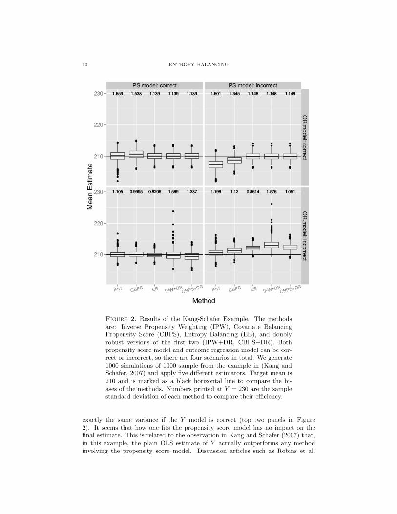
10 ENTROPY BALANCING

Figure 2. Results of the Kang-Schafer Example. The methodsare: Inverse Propensity Weighting (IPW), Covariate BalancingPropensity Score (CBPS), Entropy Balancing (EB), and doublyrobust versions of the first two (IPW+DR, CBPS+DR). Bothpropensity score model and outcome regression model can be cor-rect or incorrect, so there are four scenarios in total. We generate1000 simulations of 1000 sample from the example in (Kang andSchafer, 2007) and apply five different estimators. Target mean is210 and is marked as a black horizontal line to compare the bi-ases of the methods. Numbers printed at Y = 230 are the samplestandard deviation of each method to compare their efficiency.

exactly the same variance if the Y model is correct (top two panels in Figure2). It seems that how one fits the propensity score model has no impact on thefinal estimate. This is related to the observation in Kang and Schafer (2007) that,in this example, the plain OLS estimate of Y actually outperforms any methodinvolving the propensity score model. Discussion articles such as Robins et al.

ENTROPY BALANCING 11

(2007) and Ridgeway and McCaffrey (2007) find this phenomenon very uncommonin practice and is most likely due to the estimated inverse probability weights arehighly variable, which is a bad setting for doubly robust estimators.

Although the Kang-Schafer example is artificial and is arguably not very likelyto occur in practice, we make two comments here about entropy balancing in thisunfavorable setting for doubly robust estimators:

(1) If both T and Y models are misspecified, EB has smaller bias than theconventional “IPW+DR” or “CBPS+DR”. So EB seems to be less affectedby such unfavorable setting.

(2) When T model is correct but Y model is wrong (bottom-left panel in Figure2), EB has the smallest variance among all estimators. This supports theconclusion of our efficiency comparison of IPW and EB in Section 4.

Finally we want to notice that the same simulation setting is used in Tan (2010)to study the performance of a number of doubly robust estimators. The reader cancompare the Figure 2 with the results there. Overall, the performance of EntropyBalancing is comparable to the best estimator in Tan (2010).

References

Abadie, A. and G. W. Imbens (2006). Large sample properties of matching esti-mators for average treatment effects. Econometrica 74 (1), 235–267.

Albert, A. and J. A. Andersen (1984). On the existence of maximum likelihoodestimates in logistic regression models. Biometrika 71 (1), 1–10.

Bang, H. and J. M. Robins (2005). Doubly robust estimation in missing data andcausal inference models. Biometrics 61 (4), 962–973.

Chan, K. C. G., S. C. P. Yam, and Z. Zhang (2015). Globally efficient nonpara-metric inference of average treatment effects by empirical balancing calibrationweighting. Journal of Royal Statistical Society, Series B (Methodology) to appear.

Cover, T. M. and J. A. Thomas (2012). Elements of information theory. JohnWiley & Sons.

Deville, J.-C. and C.-E. Sarndal (1992). Calibration estimators in survey sampling.Journal of the American Statistical Association 87 (418), 376–382.

Diamond, A. and J. S. Sekhon (2013). Genetic matching for estimating causaleffects: A general multivariate matching method for achieving balance in obser-vational studies. Review of Economics and Statistics 95 (3), 932–945.

Ferwerda, J. (2014). Electoral consequences of declining participation: A naturalexperiment in austria. Electoral Studies 35 (0), 242–252.

Gneiting, T. and A. E. Raftery (2007). Strictly proper scoring rules, prediction, andestimation. Journal of the American Statistical Association 102 (477), 359–378.

Hahn, J. (1998). On the role of the propensity score in efficient semiparametricestimation of average treatment effects. Econometrica 66 (2), 315–332.

Hainmueller, J. (2011). Entropy balancing for causal effects: A multivariatereweighting method to produce balanced samples in observational studies. Polit-ical Analysis 20, 25–46.

Hastie, T. J. and R. J. Tibshirani (1990). Generalized additive models, Volume 43.CRC Press.

Hirano, K. and G. Imbens (2001). Estimation of causal effects using propensityscore weighting: An application to data on right heart catheterization. HealthServices and Outcomes Research Methodology 2, 259–278.

12 ENTROPY BALANCING

Hirano, K., G. W. Imbens, and G. Ridder (2003). Efficient estimation of averagetreatment effects using the estimated propensity score. Econometrica 71 (4),1161–1189.

Holland, P. W. (1986). Statistics and causal inference. Journal of the AmericanStatistical Association 81, 945–960.

Imai, K., G. King, and E. A. Stuart (2008). Misunderstandings between exper-imentalists and observationalists about causal inference. Journal of the RoyalStatistical Society: Series A (Statistics in Society) 171 (2), 481–502.

Imai, K. and M. Ratkovic (2014). Covariate balancing propensity score. Journal ofthe Royal Statistical Society: Series B (Statistical Methodology) 76 (1), 243–263.

Kang, J. D. and J. L. Schafer (2007). Demystifying double robustness: A compar-ison of alternative strategies for estimating a population mean from incompletedata. Statistical Science 22 (4), 523–539.

Lunceford, J. K. and M. Davidian (2004). Stratification and weighting via thepropensity score in estimation of causal treatment effects: a comparative study.Statistics in Medicine 23 (19), 2937–2960.

Marcus, J. (2013). The effect of unemployment on the mental health of spousesevidence from plant closures in germany. Journal of Health Economics 32 (3),546–558.

Neyman, J. (1923). Sur les applications de la thar des probabilities aux experiencesagaricales: Essay des principle. excerpts reprinted (1990) in english. StatisticalScience 5, 463–472.

Qin, J. and B. Zhang (2007). Empirical-likelihood-based inference in missing re-sponse problems and its application in observational studies. Journal of the RoyalStatistical Society: Series B (Statistical Methodology) 69 (1), 101–122.

Ridgeway, G. and D. F. McCaffrey (2007). Comment: Demystifying double robust-ness: A comparison of alternative strategies for estimating a population meanfrom incomplete data. Statistical Science 22 (4), 540–543.

Robins, J., M. Sued, Q. Lei-Gomez, and A. Rotnitzky (2007). Comment: Perfor-mance of double-robust estimators when inverse probability weights are highlyvariable. Statistical Science 22 (4), 544–559.

Robins, J. M., A. Rotnitzky, and L. Zhao (1994). Estimation of regression coeffi-cients when some regressors are not always observed. Journal of the AmericanStatistical Association 89, 846–866.

Rosenbaum, P. and D. Rubin (1983). The central role of the propensity score inobservational studies for causal effects. Biometrika 70 (1), 41–55.

Rosenbaum, P. and D. Rubin (1984). Reducing bias in observational studies usingsubclassification on the propensity score. Journal of the American StatisticalAssociation 79, 516–524.

Rosenbaum, P. R. and D. B. Rubin (1985). Constructing a control group usingmultivariate matched sampling methods that incorporate the propensity score.The American Statistician 39 (1), 33–38.

Rubin, D. (1974). Estimating causal effects of treatments in randomized and non-randomized studies. Journal of Educational Psychology 66 (5), 688–701.

Sarndal, C.-E. and S. Lundstrom (2005). Estimation in surveys with nonresponse.John Wiley & Sons.

Silvapulle, M. J. (1981). On the existence of maximum likelihood estimators forthe binomial response models. Journal of the Royal Statistical Society. Series B

ENTROPY BALANCING 13

(Methodological) 43 (3), 310–313.Stefanski, L. A. and D. D. Boos (2002). The Calculus of M-Estimation. The

American Statistician 56 (1), 29–38.Tan, Z. (2006). A distributional approach for causal inference using propensity

scores. Journal of the American Statistical Association 101, 1619–1637.Tan, Z. (2010). Bounded, efficient and doubly robust estimation with inverse weight-

ing. Biometrika 97 (3), 661–682.Wang, Q. and J. N. K. Rao (2002). Empirical likelihood-based inference under

imputation for missing response data. The Annals of Statistics 30 (3), 896–924.Zhao, Q. (2016). Covariate balancing propensity score by tailored loss functions.Zubizarreta, J. R. (2015). Stable weights that balance covariates for estimation

with incomplete outcome data. Journal of the American Statistical Associa-tion 110 (511), 910–922.

Appendix A. Theoretical proofs

We first describe the conditions under which the EB problem (3) admits a so-lution. The existence of wEB depends on the solvability of the moment matchingconstraints

(14)∑Ti=0

wicj(Xi) = cj(1), j = 1, . . . , p, w > 0,∑Ti=0

wi = 1.

As one may expect, this is closely related to the existence condition of maximumlikelihood estimate of logistic regression (Silvapulle, 1981; Albert and Andersen,1984). An easy way to obtain such condition is through the dual problem of (8)

(15)

maximizew

−n∑i=1

[wi logwi + (1− wi) log(1− wi)]

subject to∑Ti=0

wicj(Xi) =∑Ti=1

wicj(Xi), j = 1, . . . , p,

0 < wi < 1, i = 1, . . . , n.

Thus, the existence of θMLE is equivalent to the solvability of the constraints in(15), which is the overlap condition first given by Silvapulle (1981).

Intuitively, in the space of c(X), the solvability of (14) or the existence of wEB

means there is no hyperplane separating c(Xi)Ti=0 and c(1). In contrast, thesolvability of (15) or the existence of wMLE means there is no hyperplane separat-ing c(Xi)Ti=0 and c(Xi)Ti=1. Hence the existence of EB requires a strongercondition than the logistic regression MLE.

The next proposition suggests that the existence of wEB and hence wMLE isguaranteed by Assumption 2 (overlap) with high probability.

Proposition 1. Suppose Assumption 2 (overlap) is satisfied and the expectationof c(X) exist, then P(wEB exists)→ 1 as n→∞. Furthermore,

∑ni=1(wEB

i )2 → 0in probability as n→∞.

Proof. Since the expectation of c(X) exist, the weak law of large number says

c(1)p→ c∗(1) = E[c(X)|T = 1]. Therefore

Lemma 1. For any ε > 0, P(‖c(1)− c∗(1)‖∞ ≥ ε)→ 0 as n→∞.

14 ENTROPY BALANCING

Now condition on ‖c(1) − c∗(1)‖∞ ≥ ε, i.e. c(1) is in the box of side length 2εcentered at c∗(1), we want to prove that with probability going to 1 there exists wsuch that wi > 0,

∑Ti=0 wi = 1 and

∑Ti=0 wic(Xi) = c(1). Equivalently, this is

saying the convex hull generated by c(Xi)Ti=0 contains c(1). We indeed prove astronger result:

Lemma 2. With probability going to 1 the convex hull generated by c(Xi)Ti=0

contains the box Bε(c∗(1)) = c(x) : ‖c(x)− c∗(1)‖∞ ≤ ε for some ε > 0.

Proposition 1 follow immediately from Lemma 1 and Lemma 2. Now we proveLemma 2. Denote the sample space of X by Ω(X). Assumption 2 (overlap) impliesc∗(1) hence Bε(c

∗(1)) is in the interior of the convex hull of Ω(X) for sufficientlysmall ε. Let Ri, i = 1, . . . , 3p, be the 3p boxes centered at c∗(1)+ 3

2εb, where b ∈ Rpis a vector that each entry can be −1, 0, or 1. It is easy to check that the sets Ri aredisjoint and the convex hull of xi3

p

i=1 contains Bε(c∗(1)) if xi ∈ Ri, i = 1, . . . , 3p.

Since 0 < P (T = 0|X) < 1, ρ = mini P(X ∈ Ri|T = 0) > 0. This implies

(16)

P(∃Xi ∈ Ri and Ti = 0, ∀i = 1, . . . , 3p) ≥ 1−3p∑i=1

P(X 6∈ Ri|T = 0)n

≥ 1− 3p(1− ρ)n

→ 1

as n → ∞. This proves the lemma because the event in the left hand side impliesthe convex hull generated by c(Xi)Ti=0 contains the desired box. Note that (16)also tells us how many samples we actually need to ensure the existence of wEB.Indeed if n ≥ ρ−1(p log 2 + log δ−1) ≥ log(1−ρ)(δ2

−p), then the probability in (16)

is greater than 1− δ. Usually we expect δ = O(3−p). If this is the case, the numberof samples needed is n = O(p · 3p)1.

Now we turn to the second claim of the proposition, i.e.∑Ti=0 w

2ip→ 0. To prove

this, we only need to find a sequence (with respect to growing n) of feasible solutionsto (3) such that maxi wi → 0. This is not hard to show, because the probability in(16) is exponentially decaying as n increases. We can pick n1 ≥ N(δ, p, ρ) such thatthe probability of the convex hull of xin1

i=1 contains Bε(c∗(1)) is at least 1−δ, then

pick ni+1 ≥ ni + 3iN(δ, p, ρ) so the convex hull of xini+1

i=ni+1 contains Bε(c∗(1))

with probability at least 1 − 3iδ. This means for each xini+1

i=ni+1, i = 0, 1, . . .,

we have a set of weights wini+1

i=ni+1 such that∑ni+1

i=ni+1 wixi = c(1). Now supposenk ≤ n < nk+1, the choice wi = wi/k if i ≤ nk and wi = 0 if i > nk satisfiesthe constraints and maxi wi ≤ k. As n → ∞, this implies maxi wi → 0 and hence∑i w

2i → 0 with probability tending to 1.

Now we turn to the main theorem of the paper (Theorem 1). The first claim inTheorem 1 follows immediately from the following lemma:

Lemma 3. Under the assumptions in Theorem 1 and suppose logit(P [T = 1|X]) =∑pj=1 θ

∗j cj(X), then as n→∞, θEB p→ θ∗. As a consequence,

E

[∑Ti=0

wEBi Yi

]p→ E[Y (0)|T = 1].

1Note that this naive rate can actually be greatly improved by Wendel’s theorem in geometricprobability theory.

ENTROPY BALANCING 15

Proof. The proof is a standard application of M-estimation (more precisely Z-estimation) theory. We will follow the estimating equations approach described

in (Stefanski and Boos, 2002) to derive consistency of θEB. First we note the firstorder optimality condition of (7) is

(17)

n∑i=1

(1− Ti)e∑p

k=1 θkck(Xi)(cj(Xi)− cj(1)) = 0, j = 1, . . . , R.

We can rewrite (17) as estimating equations. Let φj(X,T ;m) = T (cj(X)−mj), j =1, . . . , R and ψj(X,T ; θ,m) = (1− T ) exp

∑pk=1 θkck(X)(cj(X)−mj), then (17)

is equivalent to

(18)

n∑i=1

φj(Xi, Ti;m) = 0, j = 1, . . . , R,

n∑i=1

ψj(Xi, Ti; θ,m) = 0, j = 1, . . . , R.

Since φ(·) and ψ(·) are all smooth functions of θ and m, all we need to verify isthat m∗j = E[cj(X)|T = 1] and θ∗ is the unique solution to the population versionof (18). It is obvious that m∗ is the solution to E[φj(X,T ;m)] = 0, j = 1, . . . , R.Now take conditional expectation of ψj given X:

E[ψj(X,T ; θ,m∗) |X] = (1− e(X))e∑p

k=1 θkck(X)(cj(X)−m∗j )

=

(1− e

∑pk=1 θ

∗kck(X)

1 + e∑p

k=1 θ∗kck(X)

)e∑p

k=1 θkck(X)(cj(X)−m∗j )

=e∑p

k=1 θkck(X)

1 + e∑p

k=1 θ∗kck(X)

(cj(X)− E[cj(X)|T = 1]).

The only way to make E[ψj(X,T ; θ,m∗)] = 0 is to have

e∑p

k=1 θkck(X)

1 + e∑p

k=1 θ∗kck(X)

= const · P(T = 1|X),

i.e. θ = θ∗. This proves the consistency of θEB.The consistency of γEB is proved by noticing

wEBi =

exp(∑pj=1 θ

EBj cj(Xi))∑

Ti=0 exp(∑pj=1 θ

EBj cj(Xi))

p→ P (Ti = 1|Xi)

1− P (Ti = 1|Xi),

which is the IPW-NR weight defined in (2).

The second claim is a corollary of Theorem 2, which is proved below. For simplic-ity we denote ξ = (mT , θT , µ(1|1), γ)T and the true parameter as ξ∗. Throughoutthis section we assume logit(e(X)) =

∑pj=1 θ

∗j cj(X). Denote c(X) = c(X)− c∗(1),

e∗(X) = e(X; θ∗), l∗(X) = exp∑pj=1 θ

∗j cj(X) = e∗(X)/(1− e∗(X)). Let

φj(X,T ;m) = T (cj(X)−mj), j = 1, . . . , p,

ψj(X,T ; θ,m) = (1− T )e∑p

k=1 θkck(X)(cj(X)−mj), j = 1, . . . , p,

ϕ1|1(X,T, Y ;µ(1|1)) = T (Y − µ(1|1)),

ϕ(X,T, Y ; θ, µ(1|1), γ) = (1− T )e∑p

j=1 θjcj(X)(Y + γ − µ(1|1)),

16 ENTROPY BALANCING

and ζ(X,T, Y ;m, θ, µ(1|1), γ) = (φT , ψT , ϕ1|1, ϕ)T be all the estimating equations.

The Entropy Balancing estimator γEB is the solution to

(19)1

n

n∑i=1

ζ(Xi, Ti, Yi;m, θ, µ(1|1), γ) = 0.

There are two forms of “information” matrix that need to be computed. Thefirst is

AEB(ξ∗) = E

[−

∂

∂ξTζ(X,T, Y ; ξ∗)

]=

(E

[−

∂

∂mTζ(ξ∗)

]E

[−

∂

∂θTζ(ξ∗)

]E

[−

∂

∂µ(1|1)ζ(ξ∗)

]E

[−∂

∂γζ(ξ∗)

])

= E

T ·IR 0 0 0(1−T )l∗(X)·IR −(1−T )l∗(X)(c(X)−c∗(1))c(X)T 0 0

0T 0T T 0

0 −(1−T )l∗(X)(Y (0)−µ∗(0|1))c(X)T (1−T )l∗(X) −(1−T )l∗(X)

= π ·

IR 0 0 0

IR −Cov[c(X)|T = 1] 0 00T 0T 1 0

0 −Cov(Y (0), c(X)|T = 1) 1 −1

.

A very useful identity in the computation of the expectation is

E[f(X,Y )|T = 1] = π−1E[e(X)f(X,Y )]

=P(T = 0)

π· E[

e(x)

1− e(X)f(X,Y )

∣∣∣∣T = 0

].

The second information matrix is the covariance of ζ(X,T, Y ; ξ∗). Denote Y (t) =Y (t)− µ∗(t|1), t = 0, 1

BEB(ξ∗) = E[ζ(X,Y, T ; ξ∗)ζ(X,Y, T ; ξ∗)T ]

= E

T c(X)c(X)T 0 T Y (1)c(X) 0

0 (1−T )l∗(X)2c(X)c(X)T 0 (1−T )l∗(X)2Y (0)c(X)

T Y (1)c(X)T 0T T Y 2(1) 0

0 (1−T )l∗(X)2Y (0)c(X)T 0 (1−T )l∗(X)2Y 2(0)

.

The asymptotic distribution of γEB is N(γ, V EB(ξ∗)/n) where V EB(ξ∗) is thebottom right entry of AEB(ξ∗)−1BEB(ξ∗)AEB(ξ∗)−T . Let’s denote

Ha1,a2 = Cov(a1, a2|T = 1),

Ga1,a2 = E[l∗(X)(a1 − E[a1|T = 1])(a2 − E[a2|T = 1])T |T = 1

]T,

and Ha = Ha,a, Ga = Ga,a. So

AEB(ξ∗) = π ·

IR 0 0 0IR −Hc(X) 0 00T 0T 1 00 −HY (0),c(X) 1 −1

,

AEB(ξ∗)−1 = π−1 ·

IR 0 0 0

H−1c(X) −H−1

c(X) 0 0

0T 0T 1 0−HT

c(X),Y (0)H−1c(X) HT

c(X),Y (0)H−1c(X) 1 −1

,

ENTROPY BALANCING 17

and

BEB(ξ∗) = π ·

Hc(X) 0 Hc(X),Y (1) 0

0 Gc(X) 0 Gc(X),Y (0)

HY (1),c(X) 0T HY (1) 00 GTY (0),c(X) 0 GY (0)

.

Thus

V EB = π−1 ·HTc,0H

−1c

(Hc,0 +GcH

−1c Hc,0 − 2Gc,0 − 2Hc,1

)+H1 +G0

.

It would be interesting to compare V EB(ξ∗) with V IPW(ξ∗), the asymptotic vari-ance of γIPW. The IPW PATT estimator (2) is equivalent to solving the followingestimating equations

n∑i=1

(Ti −

1

1 + e−∑p

k=1 θkck(Xi)

)cj(Xi) = 0, r = 1, . . . , R,

1

n

n∑i=1

ϕ1|1(Xi, Ti, Yi; θ, µ(1|1), γ) = 0,

1

n

n∑i=1

ϕ(Xi, Ti, Yi; θ, µ(1|1), γ) = 0.

If we call Ka1,a2 = E[(1− e(X))a1aT2 |T = 1], we have

AIPW(ξ∗) = E

e∗(X)(1−e∗(X))c(X)c(X)T 0 0

0T T 0

−(1−T )l∗(X)Y (0)c(X)T (1−T )l∗(X) −(1−T )l∗(X)

= π ·

Kc(X) 0 0

0T 1 0

−HY (0),c(X) 1 −1

.

AIPW(ξ∗)−1 = π−1 ·

K−1c(X)

0 0

0T 1 0

−HY (0),c(X)K−1c(X)

1 −1

.

Let q∗(X) = e∗(X)l∗(X),

BIPW(ξ∗) = E

(T−e∗(X))2c(X)c(X)T T (T−e∗(X))Y (1)c(X) −(1−T )q∗(X)Y (0)c(X)

T (T−e∗(X))Y (1)c(X)T T Y 2(1) 0

−(1−T )q∗(X)Y (0)c(X) 0 (1−T )l∗(X)2Y 2(0)

= π ·

Kc(X) Kc(X),Y (1) Kc(X),Y (0)−Hc(X),Y (0)

KTc(X),Y (1)

HY (1) 0

KTc(X),Y (0)

−HTc(X),Y (0)

0 GY (0)

.

V IPW can thus be computed consequently and we omit the details.

Appendix B. Additional Simulation Example

Here we provide an additional simulation example by Lunceford and Davidian(2004) to verify claims in Theorems 1 and 2.

In this simulation, the data still consists of Xi, Zi, Ti, Yi, i = 1, . . . , n, butall of them are observed. Both Xi and Zi are three dimensional vectors. Thepropensity score is only related to X through:

logit(P(Ti = 1)) = β0 +∑j=1

βjXij .

18 ENTROPY BALANCING

Note the above does not involve elements of Zi. The response Y is generatedaccording to

Yi = ν0 +

3∑j=1

νjXij + ν4Ti +

3∑j=1

ξjZij + εi; εi ∼ N(0, 1).

The parameters here are set to be

ν = (0,−1, 1,−1, 2)T ;

β is set as:

βno = (0, 0, 0, 0)T ,

βmoderate = (0, 0.3,−0.3, 0.3)T , or

βstrong = (0, 0.6,−0.6, 0.6)T .

The choice of β depends on the level of association of T and X. ξ is based on asimilar choice on the level of association of Y and Z:

ξno = (0, 0, 0)T ,

ξmoderate = (−0.5, 0.5, 0.5)T , or

ξstrong = (−1, 1, 1)T .

The joint distribution of (Xi, Zi) is specified by taking Xi3 ∼ Bernoulli(0.2) andthen generate Zi3 as Bernoulli with

P (Zi3 = 1|Xi3) = 0.75Xi3 + 0.25(1−Xi3).

Conditional on Xi3, (Xi1, Zi1, Xi2, Zi2) is then generated as multivariate normalN(aXi3

, BXi3), where a1 = (1, 1,−1,−1)T , a0 = (−1,−1, 1, 1)T and

B0 = B1 =

1 0.5 −0.5 −0.5

0.5 1 −0.5 −0.5−0.5 −0.5 1 0.5−0.5 −0.5 0.5 1

.

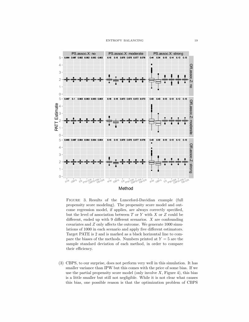
The data generating process implies the true PATT is γ = 2. Since the outcomeY depends on both X and Z, we always fit a full linear model of Y using X and Z,if such model is needed. T only depends on X, so it is not necessary to include Zin propensity score modeling. However, as pointed out by Lunceford and Davidian(2004, Sec. 3.3), it is actually beneficial to “overmodel” the propensity score byincluding Z in the model. Here we will try both possibilities, the “full” modelingof T using both X and Z, and the “partial” modeling of T using only X.

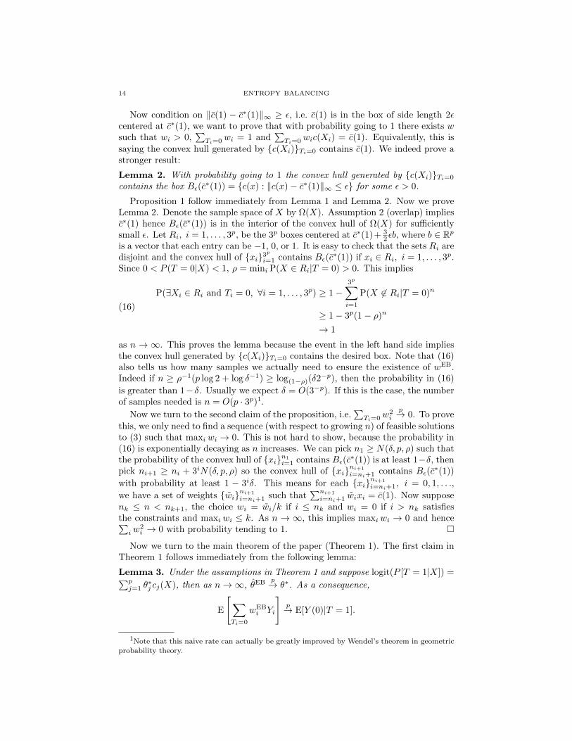
We generated 1000 simulated data sets and the results are shown in Figure 3for “full” propensity score modeling and Figure 4 for “partial” propensity scoremodeling. We make the following comments about these two plots:

(1) IPW and all the other estimators are always consistent, no matter whatlevel of association is specified. This is because the propensity score modelis always correctly specified.

(2) When using full propensity score modeling, all the doubly robust estimators(EB, IPW+DR, CBPS+DR and EB+DR) have almost the same samplevariance. This is because all of them are asymptotically efficient.

ENTROPY BALANCING 19

Figure 3. Results of the Lunceford-Davidian example (fullpropensity score modeling). The propensity score model and out-come regression model, if applies, are always correctly specified,but the level of association between T or Y with X or Z could bedifferent, ended up with 9 different scenarios. X are confoundingcovariates and Z only affects the outcome. We generate 1000 simu-lations of 1000 in each scenario and apply five different estimators.Target PATE is 2 and is marked as a black horizontal line to com-pare the biases of the methods. Numbers printed at Y = 5 are thesample standard deviation of each method, in order to comparetheir efficiency.

(3) CBPS, to our surprise, does not perform very well in this simulation. It hassmaller variance than IPW but this comes with the price of some bias. If weuse the partial propensity score model (only involve X, Figure 4), this biasis a little smaller but still not negligible. While it is not clear what causesthis bias, one possible reason is that the optimization problem of CBPS

20 ENTROPY BALANCING

Figure 4. Results of the Lunceford-Davidian example (partialpropensity score modeling). The settings are exactly the same asFigure 3 except the methods here don’t use Z in their propensityscore models.

is nonconvex, so the local solution which is used to construct γ estimatorcould be far from the global solution. Another possibility is that CBPSuses GMM or Empirical Likelihood to combine likelihood with imbalancepenalty, which is less efficient than maximum likelihood directly. Thus,although the estimator is asymptotically unbiased, the convergence spendto the true γ is quite slower than IPW. CBPS combined with outcomeregression (CB+DR) fixes the bias and inefficiency issue occurred in CBPSwithout outcome regression.

(4) EB, in contrast, performs quite well in this simulation. It has relativelysmall variance overall, especially if we use the “full” model, i.e. both X andZ are being balanced in (3).

ENTROPY BALANCING 21

(5) The difference between EB and EB+DR is that while EB only balances“partial” or “full” covariates, EB+DR additionally combines a outcomelinear regression model on all the covariates. As shown in the first proofof Theorem 1, when the “full” covariates are used, EB is exactly the sameas EB+DR. We can observe this from Figure 3. When EB only balances“partial” covariates, the two methods are different and indeed EB+DR ismore efficient in Figure 4 since it fits the correct Y model.

(6) Using the “full” propensity score model improves the efficiency of pureweighting estimators (IPW, CBPS and EB) a lot, but has very little impacton estimators that involves an outcome regression model (IPW+DR andCBPS+DR) compared to ”partial” propensity score modeling. AlthoughEB could be viewed as fitting a outcome model implicitly, the ”partial” EBestimator only uses X in the outcome model, that is precisely the reasonwhy it is not efficient. Thus there are both robustness and efficiency reasonsthat one should include all relevant covariates in EB, even if the covariatesaffect only one of T and Y .