Quality and Advertising in a VerticallyDifferentiated Market

Zsolt Katona and Elie Ofek ∗

May 26, 2008

∗Zsolt Katona is a Ph.D. candidate at INSEAD, Bd. de Constance, 77305, Fontainebleau, France.E-mail: zsolt.katona@insead.edu. Tel.: +33 1 60 72 92 26 Fax: +33 1 60 74 55 00. Elie Ofek is As-sociate Professor of Business Administration at the Harvard Business School, eofek@hbs.edu, Tel.:+1 617 495 6301. The authors thank Miklos Sarvary, David Soberman, Timothy Van-Zandt, par-ticipants of the marketing track at the INFORMS 2007 Annual Meeting, and seminar participantsat UT Dallas for valuable suggestions.

Quality and Advertising in a Vertically DifferentiatedMarket

Abstract

We examine firms’ quality positions when consumers can only consider purchasing prod-

ucts that they are informed about through advertising. Consumers compare the alternatives

in their consideration set and choose the product that maximizes their utility net of price.

Firms choose product quality in a first stage, advertising strategy in a second stage, and

prices in the last stage. We study two forms of advertising– blanket and targeted. Under

blanket advertising, firms communicate indiscriminately and a consumer’s probability of see-

ing an ad depends on the level of ad expenditure. We find that when blanket advertising

is relatively ineffective, i.e., it is costly to ensure that all consumers are informed, both

firms choose a light ad spending. This allows the firms to be relatively undifferentiated in

qualities, without concern of intense price competition. When blanket advertising is very

effective, the high quality firm expends heavily on advertising, while its rival differentiates

with a low quality product and expends lightly on advertising. Interestingly, in a mid range

of advertising effectiveness one firm chooses a high quality product and its rival positions

close by. In this way, the lower quality firm induces its rival to advertise only lightly to avoid

fierce price competition. Under targeted advertising, firms choose the specific segment(s)

they wish to inform. We identify conditions such that both firms choose equally high quality

products, but advertise to different segments. This can result in a middle pocket of unserved

consumers, even though consumers with lower willingness to pay are served.

(Product Quality, Advertising Strategy, Differentiation, Competition)

1 Introduction

In order for consumers to consider the purchase of a product, they must first be aware of

its existence and informed about its characteristics.1 Although there are a number of ways

for consumers to become informed about the products available in the marketplace, firm

initiated communications are a primary vehicle. In some cases, firms can be selective and

send messages only to those consumers who are part of their target market. For example,

by purchasing or compiling a list of consumers that meet certain criteria, firms can send

targeted e-mails or direct mail; in B2B settings firms can send their sales force to a subset

of potential customers with common characteristics. In other cases, firms cast a much wider

net and use media outlets that preclude direct control over who sees their ads. For example,

by running a commercial on national TV or placing an ad in a general interest magazine, a

firm will potentially reach a broad set of consumers. It is noteworthy that in the U.S. alone

companies spent over $155 billion in 2006 to advertise their offerings to consumers.2

Consumers consider the various products they are informed about and choose the one

that delivers them maximum utility. Consequently, the return on advertising for a firm will

critically depend on how its offering compares to the other offerings in the marketplace and

how aggressively those products are advertised, i.e., which products constitute consumers’

consideration set. In this context, the decision of what quality product to offer and then

how heavily to promote it through advertising become intertwined, and further depend on

the rival’s product positioning and advertising strategy.

For example, in any given automobile class (such as sedans, sports utility, roadsters)

manufacturers need to make decisions on the quality of their models prior to development.

Upon launch, these manufacturers (e.g., Mazda, BMW, Porsche) need to advertise their cars

to engender demand. High-tech firms, such as manufacturers of storage hardware, decide

whether to position their devices as suitable for the high- or low-end spectrum of computing

needs, and their sales force must then communicate these positions to relevant customers. In

several beverage categories the same is true. For instance, firms that market ground coffee

1Behavioral models of the consumer’s decision making process (DMP) typically include the stages ofawareness, knowledge, consideration/evaluation, preference and ultimately purchase (Dolan 1999, Kellerand Kotler 2006).

2Advertising Age, June 25, 2007.

2

(e.g., Maxwell House, Foldger’s, Cafe de Columbia) select the quality of beans to use and

determine how finely they will be roasted prior to expending resources on promotion; firms

that produce vodka (e.g., Smirnoff, Absolut, Russian Standard) make decisions on the type

of grains to be used and on the consistency of the distilling process, and subsequently carry

out advertising campaigns to inform consumers.

In this paper, we study how the need to advertise in order to be included in the con-

sumer’s consideration set affects a firm’s decision of where to position its product vis-a-vis

the competition. We develop a duopoly model in which firms choose product quality in

a first stage, their advertising strategy in a second stage, and set prices in the last stage.

Consumers are heterogeneous with respect to their valuation for quality, allowing for vertical

differentiation.

We study two forms of advertising that firms can use to inform consumers about the ex-

istence (and characteristics) of their products. The first type– blanket advertising– captures

situations where firms communicate to all consumers indiscriminately (e.g., during widely

popular shows on broadcast television or radio). The probability that a firm’s product enters

a consumer’s consideration set is a function of the advertising expenditure. Specifically, a

heavy ad spend guarantees that all consumers will receive the firm’s message and consider

its product, while a light ad spend only results in a likelihood that each consumer receives

the message. Three main equilibria can emerge depending on the effectiveness of blanket

advertising, which is a function of the cost differential between heavy and light advertising

expenditures (i.e., the more it costs to advertise heavily the less effective advertising is).

When advertising is relatively ineffective, the return on advertising heavily is small and both

firms advertise lightly. Price competition is softened because the likelihood that a given

consumer receives ads from both firms is low; hence one firm selects maximal quality and its

rival can also choose a relatively high quality, leading to a moderate level of quality differen-

tiation. When, at the other extreme, blanket advertising is very effective, one firm chooses

maximal quality and expends heavily on advertising. The rival now prefers to differentiate

with a much lower quality product and to expend lightly on advertising to avoid harsh price

competition. In a mid range of advertising effectiveness, we get the intriguing result that by

choosing quality appropriately, the lower-quality firm induces the high-quality firm to expend

3

only lightly on advertising. Specifically, because the products are minimally differentiated,

the high-quality firm seeks to avoid fierce price competition by refraining from advertising

heavily. Somewhat counterintuitively, the more effective advertising is in this range the less

quality differentiation is observed.

The second type of advertising we examine–targeted advertising –captures situations

where firms can communicate to specific segment(s) they wish to inform about their product.

We characterize equilibria where each firm advertises to a distinct segment. Because each

consumer only considers one product, the firms do not compete in the pricing stage and

hence both choose equally high quality– that is, their products are entirely undifferentiated.

Interestingly, due to the relatively high prices firms charge, there exist conditions such that

a set of consumers with moderate valuation for quality are unserved, even though consumers

in a different segment with lower willingness to pay are served. We also show that the total

number of consumers served follows an inverted-U shape as a function of the size of the low

willingness-to-pay segment.

In an extension, we study the role of persuasive advertising. While the two types of

informative advertising impact awareness and consideration, persuasive advertising changes

the way consumers perceive product quality; thereby affecting their willingness to pay. Our

main result here is that firms may differentiate less in objective qualities than under no ad-

vertising. However, the difference in their persuasive advertising levels counterbalances this

effect, leading to the same degree of differentiation in perceived qualities as when consumers

are fully aware of objective product qualities.

The rest of the paper is organized as follows. The next section relates our work to

the relevant literature and summarizes our contribution. Section 3 sets up the basics of

the model in terms of demand and firm behavior. Section 4 solves the case of blanket

advertising and Section 5 solves the case of targeted advertising. We consider the persuasive

advertising extension in Section 6. Finally, Section 7 concludes, discusses limitations and

outlines opportunities for future research. To enhance readability, we postpone all proofs to

the Appendix.

4

2 Related Literature

Our work is primarily related to the vertical differentiation literature, beginning with the

widely known model of Shaked and Sutton (1982). They examine price competition between

firms that first choose the quality of the products they sell. Since consumers, who are

fully informed about product qualities, are heterogeneous with respect to their valuation of

quality, in equilibrium firms choose different qualities in order to reduce price competition

in the last stage. Moorthy (1988) relaxes Shaked and Sutton’s zero cost of production

assumption by introducing a quadratic cost function for quality, resulting in an equilibrium

where the firm choosing the lower quality may be better off. Moorthy (1988) further shows

that when firms choose qualities (simultaneously or sequentially) the equilibrium strategies

are to differentiate in qualities. Assuming that firms do not cover the market, Choi and

Shin (1992) show that the low quality firm will choose a quality level which is a fixed

proportion of the high quality firm’s choice. Wauthy (1996) on the other hand, gives a full

characterization of quality choices, allowing the coverage of the market to be endogenous.

More recently, Choudhary et al. (2005) and Jing (2006) both find that the higher quality firm

can be worse off in equilibrium. Choudhary et al. (2005) examine a vertical differentiation

model where personalized pricing is allowed. Personalized pricing results in greater market

coverage, but also intensifies competition, which can hurt the high quality firm. Jing (2006)

identifies the conditions on the cost structure under which producing the low-quality good

is more profitable.

The previous studies show that quality differentiation is a robust equilibrium outcome.

However, in reality similar quality products are often observed in the marketplace. Rhee

(1996) cites evidence for this and offers an explanation that incorporates consumer hetero-

geneity along unobservable attributes into the vertical differentiation model. As a result, if

consumers are sufficiently heterogeneous on the extra dimensions, in equilibrium firms offer

products that are identical on the observed quality dimensions (but differentiated on the un-

observed dimensions). Banker et al. (1998) investigate the relationship between equilibrium

quality levels and the intensity of competition between firms. They find that the degree of

differentiation depends on the market structure and production cost differences.

Notably, the papers in this stream analyze firms’ quality positions under various price

5

and cost assumptions, but assume that all consumers are fully informed about these qualities

and ignore the role or need for advertising.

Another stream of literature related to our work is the vast amount of studies on adver-

tising. We focus on prior research that examines the relationship between advertising and

product quality. It is theoretically well-established in economics and marketing that adver-

tising level can be a signal of quality (Nelson 1974, Milgrom and Roberts 1986). However,

this work ignores the informativeness of advertising and thus its effect on market size. In

contrast, Zhao (2000) shows that when advertising raises awareness, spending less can be the

optimal signaling approach of the high-quality firm. Iyer et al. (2005), on the other hand,

investigate how firms should target their advertising when consumers have horizontal tastes.

They find that firms advertise more to consumers who have a strong preference for their

product, and argue that this is a way to soften price competition. For the most part, the

literature in this stream takes product qualities as exogenous.

Our contribution lies in extending the first stream of literature by exploring the strategic

interaction between advertising spending and quality choice and by showing how advertising

can lead to less or even no differentiation. Relative to the second stream, we endogenize

product qualities and analyze how this decision is impacted by foreseeing the need to adver-

tise. In this context, we employ models where advertising impacts consumer consideration

of products either at the general (blanket) or specific (targeted) reach level.

3 Model Setup

We assume that there are two competing firms that seek to sell their products in a given

market. We index the firms by the numbers 1 and 2 or the letters i and j, always assuming

that i 6= j. If firms offer different quality products, we denote the firm offering the lower

quality product by 1 and the higher quality product by 2. We assume that every consumer

purchases at most one unit of the product. We further assume that consumers are heteroge-

neous with respect to their valuation of quality, denoted by ϑ. The parameter ϑ is uniformly

distributed in the interval I = [0, 1]. A consumer with parameter ϑ gains utility ϑs− p from

a product with quality s priced at p, and purchases the product for which his/her utility is

greater. However, consumers can only consider purchasing products they are informed about

6

(Keller and Kotler 2006). By advertising, a firm communicates the existence and character-

istics of its product (including price), thereby affecting the likelihood that its product enters

a consumer’s consideration set. Our characterization is thus consistent with the informative

view of advertising (see, e.g., Tirole 1988, Iyer et al. 2005, and references therein).3 In

Section 7.1 we discuss our assumptions on the impact of advertising and possible extensions

to consumers’ knowledge about products (e.g., through search).

We study two different types of informative advertising mechanisms. In the first type,

which we call blanket advertising, the probability that a consumer considers firm i’s product

is ai, independently for each consumer. This probability depends on how heavily firm i

advertises and is independent of firm j’s advertising level. In the second type, which we call

targeted advertising, firms can communicate to subsets of consumers that belong to distinct

segments. If a consumer is in a firm’s targeted segment, s/he considers that firm’s product

with probability 1.

Timing

The timing of the game is as follows. First, firms choose their qualities si (s1 ≤ s2). Qualities

are positive and have a maximum value that is normalized to 1. Second, firms make their

advertising decisions, and incur the associated promotion costs. In the blanket case they

set their advertising level and in the targeted advertising case they choose the segment(s)

they wish to advertise to. Third, firms set prices. Finally, consumers make their purchases.

This timing reflects the notion that quality choice tends to be a long-term decision, whereas

prices can be easily changed. The time-scope of advertising decisions is somewhere in be-

tween; consistent with this timing, in practice advertising budget is typically set only after

the product characteristics have been determined.

3Consistent with consumer behavior research (e.g., Mitra and Lynch 1995), the role of advertising in ourmodel can also be regarded as creating awareness or a trigger for the consumer to include a given productin their consideration set. Trivially, an individual cannot consider buying a product that s/he is not awareof. Yet the consideration set can be narrower than the set of products the consumer is aware of, since someof these products might be excluded before carefully comparing the utilities derived from them (Hauser andWernerfelt 1990). For example, because advertising impacts the salience of products and their characteristicsin consumers’ memory, it affects which products are “top of mind” at the time of purchase (Iyer et al. 2005,provide an excellent discussion of this issue). Hence, our model applies even if we assume that consumersare aware of all products; all we require for our results to go through is that advertising sufficiently increasesthe likelihood of a product being part of the consumer’s consideration set.

7

Costs and Profits

We assume no fixed entry costs, hence both firms participate in the market. Furthermore,

we assume that variable costs are constant and normalize them to zero. Our model is thus

consistent with Shaked and Sutton (1982).4 However, advertising costs, denoted c(·), de-

pend on the advertising level chosen in the following way. In the blanket advertising case,

we assume that c(ai) is an increasing function of ai (i.e., to achieve a higher likelihood of

being considered, a firm has to spend more on advertising). In the targeted advertising case,

we assume that the cost is a linear function of the segment size. Firms’ profits are therefore

simply their revenues (price × quantity sold) minus advertising costs:

Πi = piDi − cadvi .

We solve for the pure-strategy, sub-game perfect equilibria of the game. Next, we charac-

terize the equilibria in the two different cases: blanket advertising and targeted advertising

(Sections 4 and 5, respectively).

4 Blanket Advertising

In this setup, both firms advertise to the entire mass of consumers but the probability of

being included in a consumer’s consideration set depends on the effort each firm selects. For

the sake of simplicity, let us assume that there are only two levels of advertising: heavy

(H) and light (L), with costs cH > cL, respectively. The probabilities of being considered by

consumers are then 0 < aL ≤ aH = 1. That is, a firm can either choose to heavily advertise at

a high cost, thereby ensuring every consumer is informed about its product, or to advertise

lightly at a low cost, thereby expecting only a portion of consumers to be informed. We

further assume that the impact of light advertising is not too low. Formally, this means

aL > a∗, where a∗ is defined in the Appendix (proof of Claim 2). This assumption ensures

4Having a fixed cost of developing a product would not qualitatively affect our results. Our normalizingboth variable and fixed costs of production to zero might seem as an oversimplifying assumption but isdone for two reasons. First, our assumptions in this respect correspond to Shaked and Sutton (1982),allowing us to directly compare our results to theirs. Second, it allows us to focus on the strategic incentivesto differentiate in qualities when there are advertising costs involved; including production costs wouldcomplicate this analysis without providing much added insights into the questions of interest, as our resultswould hold over a certain range of cost parameters.

8

that firms don’t trivially always advertise heavily; though we will discuss (after Proposition

1) the case of very low aL.

As a benchmark, let us solve the case of a monopolist. A consumer who considers the

monopolist’s product buys it if and only if ϑsm− pm ≥ 0. That is, the monopolist’s demand

consists of consumers that are informed about the product and for which ϑ ≥ pm/sm.

Therefore,

Dm(pm, am) = (1− pm/sm)am,

where am ∈ {aL, aH}. The monopolist chooses a price to maximize its revenue, R(pm, am, sm) =

pm(1− pm/sm)am. Given am and sm, p∗m = sm/2, thus its profit can be written as

Πm(am, sm) = smam/4− c(am),

which is increasing in sm no matter what the advertising level is. Therefore, the monopolist

sets s∗m = 1 and chooses aH over aL if and only if aH−aL

4> c, where c = cH − cL. Thus, the

monopolist advertises heavily if the extra revenue that results from this level is greater than

the additional cost needed to advertise heavily rather than lightly. Said differently, if the

effectiveness of advertising heavily is above a certain threshold then the monopolist chooses

this level. We define the effectiveness of advertising as e ≡ aH−aL

cH−cL= 1−aL

c. The monopolist

chooses to advertise heavily iff e > 4.

4.1 Duopoly

Let us now turn to the duopoly case. From this point, we will assume that e > eM = 4,

which is the critical effectiveness level for a monopolist to advertise heavily. The rationale

behind focusing on this region is that if the effectiveness of advertising heavily is so meager

that even a monopolist would choose to advertise lightly, trivially, both duopolists would

also advertise lightly. Furthermore, facing a competitor, if a firm does choose to advertise

lightly in this region then we are assured that this is a result of the strategic interaction

between the firms.

We solve the game using backward induction and begin with the last stage pricing game,

treating the qualities and advertising levels as given. Fixing the qualities chosen by firms 1

and 2 at s1, s2 (recall that we use the convention whereby s1 denotes the lower-quality firm)

9

and the advertising probabilities at a1, a2, we can characterize the pricing equilibria. The

existence of a pure-strategy equilibrium will depend on how close s1 is to s2 (or how close

the ratio s1/s2 is to 1). The critical ratio of qualities necessary for the equilibrium to exist

also depends on the proportion of consumers impacted by the advertising of each firm, which

we capture through a function f(a1, a2).

Claim 1 There exists a function f(a1, a2): 0 ≤ f(a1, a2) ≤ 1, f(a1, 1) = 1 for any a1, and

f(a, a) is increasing for a ≥ 1/2, such that

1. If s1 < s2 and s1/s2 ≤ f(a1, a2), then the equilibrium prices are

p∗1 =s1(s2 − s1)(2(s2 − s1)− a2s2 + 2s1(a1 + a2 − a1a2))

4s21(1 + a1a2 − a1 − a2) + s1s2(4a1 + 4a2 − a1a2 − 8) + 4s2

2

, (1)

p∗2 =s2(s2 − s1)(2(s2 − s1) + s1(a1 + 2a2 − a1a2))

4s21(1 + a1a2 − a1 − a2) + s1s2(4a1 + 4a2 − a1a2 − 8) + 4s2

2

. (2)

2. If s1 < s2 and s1/s2 > f(a1, a2), then there is no pure-strategy equilibrium.

3. If s1 = s2, then the equilibrium prices are always zero.

As in other models with vertical consumer heterogeneity, when the firms’ qualities are

exactly the same (case 3 of the claim) the only sustainable equilibrium is that of zero pricing.

Furthermore, if the quality levels are sufficiently different (case 1 of the claim), we can

sustain a pure strategy equilibrium with positive prices. Note that here the exact prices

firms charge will depend not only on the difference between the qualities (s2 − s1) but also

on the advertising levels. The equilibrium prices in (1) and (2) directly generalize the no-

advertising model with fully informed consumers (per Shaked and Sutton 1982). The lower-

quality firm charges a lower price than its higher-quality rival (p∗1 < p∗2). Further note that

prices generally decrease with greater advertising levels due to the fact that more consumers

can compare both offerings and hence price competition intensifies (mathematically,∂p∗i∂ai

<

0,∂p∗i∂aj

< 0). However, when the qualities are very similar (yet not identical) a pure-strategy

price equilibrium does not exist (case 2 of the claim). This is because the lower-quality

firm may have an incentive to deviate from the pricing schedule in (1) and set a higher

price to serve those consumers who only consider its product and not the competitor’s. For

10

the deviation to be profitable though, it must be the case that a sufficient proportion of

consumers do not consider the high-quality firm’s product (because with both high- and

low-quality goods offered at high prices, consumers will surely prefer the former if they are

informed about it). Moreover, if the high-quality firm advertises heavily (a2 = 1 so that

f(a1, 1) = 1) a pure-strategy equilibrium always exists.

Now let us turn our attention to the second stage of the game where firms decide whether

to advertise heavily or lightly. At this stage, quality levels are already set, thus we treat

them as parameters. Since payoffs only depend on the ratio of s1 and s2 (see Appendix),

without loss of generality we may normalize s2 = 1 and fix 0 < s1 ≤ 1. Let Rililj

(s1) denote

firm i’s revenues in the pricing-stage equilibrium, if it exists, given the advertising levels

chosen li, lj ∈ {H,L} (these levels result in probabilities ai and aj of informing a consumer).

Also, let ∆1 = R1HH(s1)−R1

LH(s1) denote the gains to firm 1 of advertising heavily instead

of lightly given its rival advertises heavily, and let ∆2 = R2HL(s1)−R2

LL(s1) denote the gains

to firm 2 of advertising heavily instead of lightly given its rival advertises lightly. Recall

that the extra cost the firm has to incur when shifting from light to heavy advertising is

denoted by c = cH − cL. Clearly, the greater ∆i relative to c, the more incentive a firm has

to advertise heavily. The following claim describes the possible equilibria at the advertising

stage, denoted by (L,L), (L,H) or (H,H), where the first argument is the advertising level

chosen by the lower-quality firm and the second is the level chosen by the higher-quality

firm.

Claim 2

1. If c ≥ ∆2 and s1 ≤ f(aL, aL) then the advertising equilibrium is (L,L).

2. If ∆2 ≥ c ≥ ∆1 then the advertising equilibrium is (L,H).

3. If ∆1 ≥ c then the advertising equilibrium is (H,H).

Claim 2 reveals several interesting properties of the possible second-stage advertising

equilibria. First, if the cost of advertising heavily is high relative to the impact it will have

on generating extra revenue (c > ∆2), then both firms will advertise lightly (of course,

we require sufficient difference in qualities per Claim 1 for the equilibrium to exist; hence

11

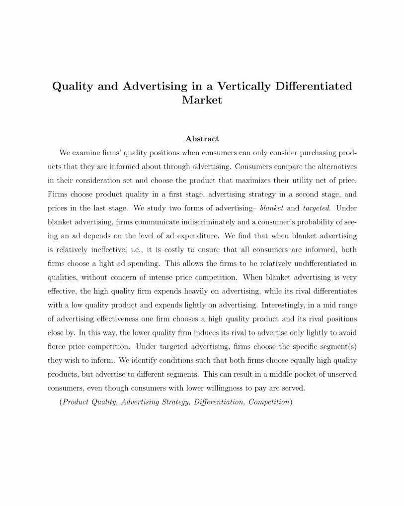
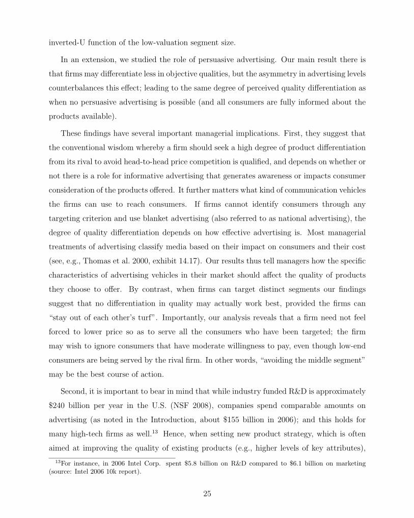
Figure 1: The Different Equilibria in the Advertising Stage as a Function of the Lower-Quality Firm’sPosition (s1) and Advertising Effectiveness (e)

the condition on s1).5 Conversely, per part 3 of Claim 2, if the cost is low relative to the

impact (c ≤ ∆1), then both firms will advertise heavily. However, for a mid-range of cost c

only the high-quality firm will advertise heavily, while the lower-quality firm will advertise

lightly. To understand the intuition for this asymmetry in advertising strategies, we note

that the return on shifting to advertising heavily is greater for the high-quality firm than

it is for the lower-quality firm (i.e., ∆2 ≥ ∆1). When consumers are informed about the

high-quality product, the supplying firm is at an advantage because of the higher willingness

to pay for its product. If the high-quality firm advertises heavily and informs all consumers,

the lower quality firm faces a tradeoff. On the one hand, advertising heavily means that

more consumers will consider its product, thus increasing its market potential. But, on

the other hand, because all consumers consider the high-quality product, the surplus that

can be extracted from these additional consumers is small as they will only purchase the

lower-quality product if it is cheap enough. Furthermore, advertising lightly softens price

competition with the high-quality firm that can then exploit the fact that some consumers

5Specifically, if c ≥ ∆2 and s1 > f(aL, aL) then there is no pure-strategy advertising equilibrium.

12

are only aware of its product. Consequently, there exists a range of costs such that only the

high-quality firm will find it beneficial to advertise heavily.

Recall that we have defined advertising effectiveness as e = (aH − aL)/c = (1 − aL)/c.

One can therefore also express the advertising equilibria in Claim 2 in terms of e. When

advertising is relatively ineffective (e < (1 − aL)/∆2) neither firm advertises heavily, when

advertising is very effective (e > (1 − aL)/∆1) both firms advertise heavily, and for mid

effectiveness values only the high-quality firm advertises heavily. Figure 1 depicts the various

equilibria in the (s1, e) space.

Having characterized the possible equilibria in the pricing and advertising sub-games, we

can now solve for the qualities chosen in the first stage.

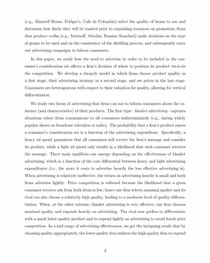
Proposition 1 There exist values e and e (eM < e < e) such that

1. For eM < e ≤ e: s1 = s and the advertising levels are (L,L).

2. For e < e < e: s1 is an increasing function of advertising effectiveness, s1 > s, and

the advertising levels are (L,L).

3. For e < e: s1 = s and the advertising levels are (L,H).

We have s2 = 1 and s > s. Equilibrium prices are given in Claim 1.

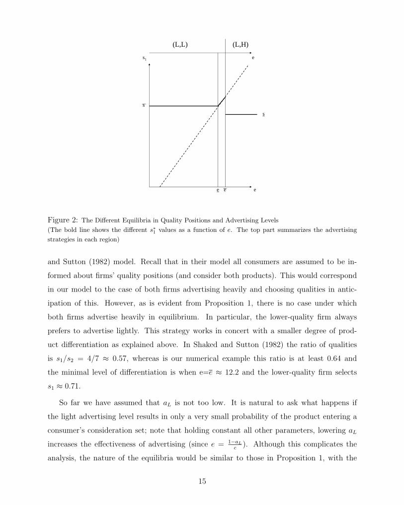
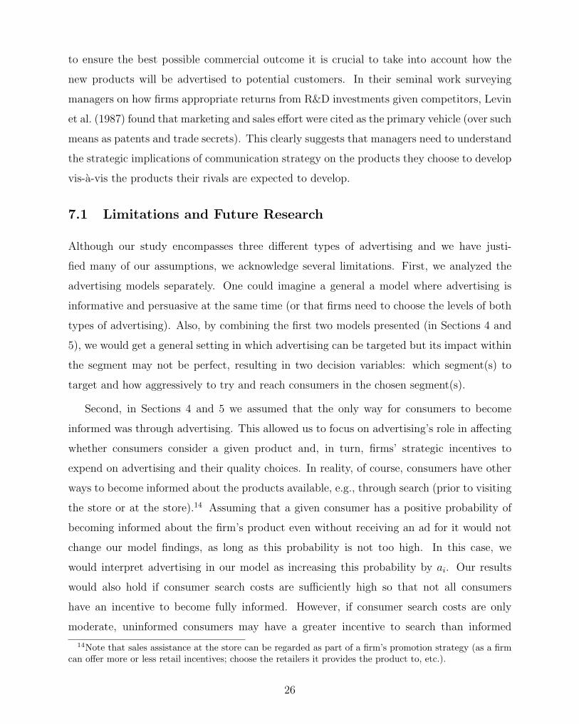
Figure 2 depicts the various equilibria in terms of the relative quality chosen by the

lower-quality firm (s1) as a function of advertising effectiveness (e). As can be gleaned, when

advertising is relatively ineffective, and consistent with Claim 2, both firms will advertise

lightly. In this case, the firm choosing a lower quality realizes that not all consumers will

be aware of the high-quality firm’s product. Thus, it can position relatively close to the

maximal quality of 1 without the fear of triggering intense price competition; resulting in

moderate quality differentiation between the firms.

At the other extreme, when advertising is effective, the high-quality firm (which always

selects a maximal quality of 1) will surely want to advertise heavily to let all consumers know

about its product. For the rival firm, advertising heavily can only be beneficial if the two

products are sufficiently differentiated. Hence, the rival firm faces a dilemma: either produce

13

a very low quality product, advertise heavily and charge a very low price, or, alternatively,

produce a moderate quality product, advertise lightly and price moderately. The latter

option is more attractive in this range given the softened price competition (the high-quality

firm need not be so aggressive as some consumers will only consider its product), and because

of the savings on advertising costs.

In the mid-region of advertising effectiveness, we get the intriguing result whereby the

best response of the lower-quality firm is to select a quality level that is increasing in ad-

vertising effectiveness. The intuition is as follows. Since advertising is somewhat effective

in this range, the high-quality firm would like to advertise heavily as its return on such ad-

vertising is quite appealing. But this is detrimental to the rival firm that would prefer some

consumers remain unaware of the high-quality option so that it can charge a high price. By

minimizing the degree of differentiation, i.e., choosing a quality level closer to 1, the rival

firm makes advertising heavily less beneficial for the high-quality firm because of the intense

price competition that would ensue (as some consumers would be informed about both prod-

ucts). Said differently, by choosing its quality appropriately, the lower-quality firm reduces

the return on advertising for the high-quality firm, and thus keeps advertising at light levels

for both. As the advertising effectiveness (e) increases, an even higher quality position needs

to be chosen in order to prevent the high-quality firm from switching to the heavy level of

advertising, which explains why∂s∗1∂e

> 0 in this region. There is clearly an upper limit to

such behavior, since we know from Claim 1 that if the firms are completely undifferentiated

then prices (and profits) will be zero. Indeed, at e = e the rival firm prefers to switch to a

much lower quality level and focus on the low willingness to pay consumers and allow the

high-quality firm to advertise heavily.6

To make the above findings more concrete, we provide the following numerical example.

Example 1 If aL = 3/4 and aH = 1, Proposition 1 describes the equilibria with e ≈ 10.5,

e ≈ 12.2 and s = 0.64, s = 0.65. The minimal level of differentiation occurs when e = e,

and s1 ≈ 0.71.

We would like to relate our findings here on product differentiation to those of the Shaked

6Consistent with Claim 1, the quality level s1 satisfies s1 < f(aL, 1) so the equilibrium exists.

14

s1

e

(L,H)(L,L)

e

s

s

e e

Figure 2: The Different Equilibria in Quality Positions and Advertising Levels(The bold line shows the different s∗1 values as a function of e. The top part summarizes the advertisingstrategies in each region)

and Sutton (1982) model. Recall that in their model all consumers are assumed to be in-

formed about firms’ quality positions (and consider both products). This would correspond

in our model to the case of both firms advertising heavily and choosing qualities in antic-

ipation of this. However, as is evident from Proposition 1, there is no case under which

both firms advertise heavily in equilibrium. In particular, the lower-quality firm always

prefers to advertise lightly. This strategy works in concert with a smaller degree of prod-

uct differentiation as explained above. In Shaked and Sutton (1982) the ratio of qualities

is s1/s2 = 4/7 ≈ 0.57, whereas is our numerical example this ratio is at least 0.64 and

the minimal level of differentiation is when e=e ≈ 12.2 and the lower-quality firm selects

s1 ≈ 0.71.

So far we have assumed that aL is not too low. It is natural to ask what happens if

the light advertising level results in only a very small probability of the product entering a

consumer’s consideration set; note that holding constant all other parameters, lowering aL

increases the effectiveness of advertising (since e = 1−aL

c). Although this complicates the

analysis, the nature of the equilibria would be similar to those in Proposition 1, with the

15

exception that for very high advertising effectiveness a new region emerges where both firms

advertise heavily (and differentiation is therefore as in Shaked and Sutton 1982). In the

extreme case of aL = 0, firms that do not set ai = aH cannot earn revenue for any level of

advertising effectiveness, and both firms advertise heavily (assuming cH is not too high).

Our findings here bear on several phenomena pertaining to vertical product differen-

tiation. First, they offer a new explanation for why in some categories we observe firms

“clustering together” in terms of quality rather than maximally differentiating to cope with

competition. Notably, the industries cited in Rhee (1996) as exhibiting this pattern are

also ones that utilize advertising. Hence, our explanation involves empirically measurable

variables directly under the firm’s control (rather than explanations that rely on unobserved

factors/attributes). Second, our findings here can shed additional light on why we observe

variance in the degree of vertical differentiation across industries and even within industry in

different product classes. The automobile industry is a case in point. In certain car categories

we observe very little quality differentiation and also limited advertising support, while in

other car categories we witness more extensive advertising spend by at least some of the

models in the class. Given that, in general, advertising is an important part of firm strategy

in automobile markets, our theory would suggest that the interaction between competitive

concerns and advertising effectiveness (impact relative to cost) can explain at least some of

this variance.7

In closing the analysis of the blanket advertising setup, the following corollary provides

the equilibrium profit levels.

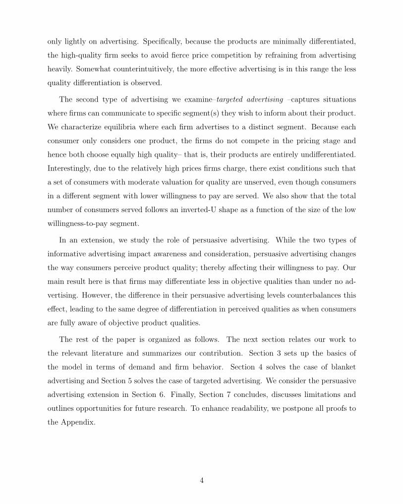
Corollary 1 The profits of the high-quality firm, π2, are a constant function of e for e ∈

[eM , e], are decreasing for e ∈ [e, e] and increasing for e > e. Profits of the lower-quality

firm, π1, are constant for e ∈ [eM , e] and e > e, and are decreasing for e ∈ [e, e].

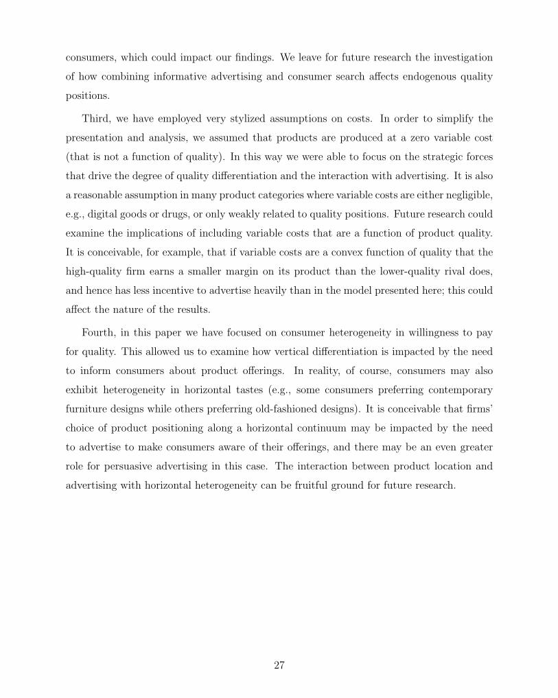
Figure 3 shows firms’ profits as a function of advertising effectiveness. Although the

firm producing the lower-quality product always makes less profits than its higher-quality

rival, the Corollary reveals a surprising phenomenon in the [e, e] interval: both firms’ profits

7For example, in the SUV category Lexus models are of higher quality than Honda models (consumerreports); the former are also more heavily advertised. In the roadster category, several models are of roughlysimilar quality (e.g., in the late 90s the BMW Z3 was regarded as having slightly lower quality than thePorsche Boxter) and were supported with less than average advertising budgets (Fournier and Dolan 1997).

16

ProfitFirm 2

ProfitFirm 1

eeeeM

Figure 3: Profits of the Two Firms as a Function of Advertising Effectiveness (e)

are decreasing functions of advertising effectiveness (e). The intuition is as follows. Recall

from Proposition 1 that in this region neither firm advertises heavily and that the degree of

quality differentiation decreases with e. Due to the firms getting closer and closer to each

other in terms of their product qualities, clearly the high-quality firm is worse off (from the

price schedules in Claim 1: as s1 → s2, p∗2 declines). The decreased differentiation is also

detrimental to the lower-quality firm, but not as much as the dramatic drop in profits it

experiences when the high-quality firm shifts to advertising heavily (see Figure 3).

5 Targeted Advertising

In this advertising setup, firms can communicate to specific segments of consumers, i.e. target

them. This gives advertisers the possibility to focus their efforts on groups of consumers.

Firms need to decide which subsets of consumers to target, and a consumer can only consider

buying a firm’s product if s/he is in a segment the firm has communicated to. In order to

focus on the targeting aspect, we assume that advertising is perfectly efficient, in the sense

that every consumer in the targeted segment is informed about the firm’s product. For the

sake of simplicity, we consider a two-segment model. Specifically, let us divide the continuum

17

of consumers into two disjunct intervals. Let the parameter 0 < t < 1 determine the two

intervals, such that consumers who are located at ϑ ≥ t belong to the high-valuation segment

and consumers who are located at ϑ < t belong to the low-valuation segment. Therefore,

the size of the low-valuation segment (denoted L) is t, whereas the size of the high-valuation

segment (denoted H) is 1− t. A firm can target neither, both, or just one of these segments.

Formally, the targeting strategy of firm i (denoted by Si) can be ∅, L, H or L ∪ H. The

costs associated with the four possible advertising strategies are 0, cL, cH, cU , respectively.

We assume that advertising costs are linear in the absolute size of the segment(s) targeted.

That is, cL∪H = cU , cL = cU t, and cH = cU(1− t). We assume that cU < t/4 to ensure that

both firms make positive profits in equilibrium. The general setup and timing of the game

are the same as those described in Section 3.

A good way to interpret this setup is that the parameter t reflects the “targeting criterion”

that the firms can use to identify consumers as having a high vs. low willingness to pay for

quality in this market.8 For example, certain demographic variables (income, education

level, etc.) can indicate which individuals are willing to pay more for certain products; those

consumers that patron certain venues (say amusement parks, or sports events) typically have

greater willingness to pay for related items.

It should be obvious that if t approaches 0 or 1, i.e., one of the segments is negligible in

size, the problem reduces to the basic vertical differentiation model of Shaked and Sutton

(1982). The following proposition shows that as long as t is not too close to either of these

extremes, then in equilibrium both firms choose maximal quality and do not differentiate.

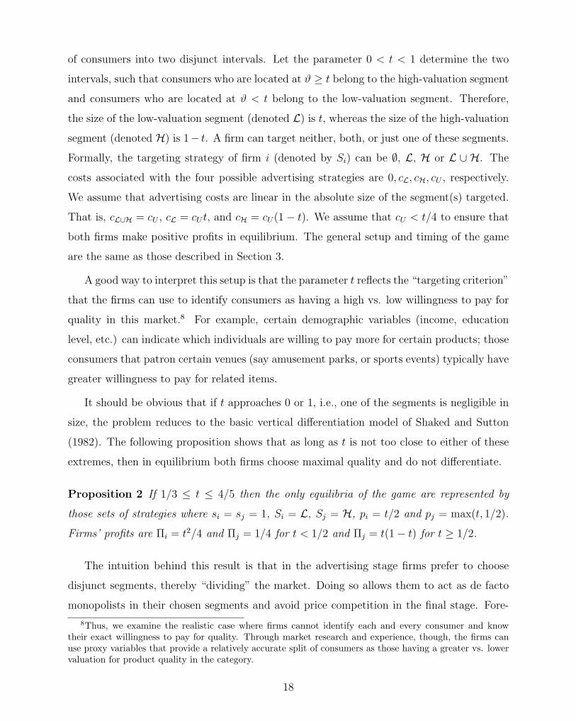
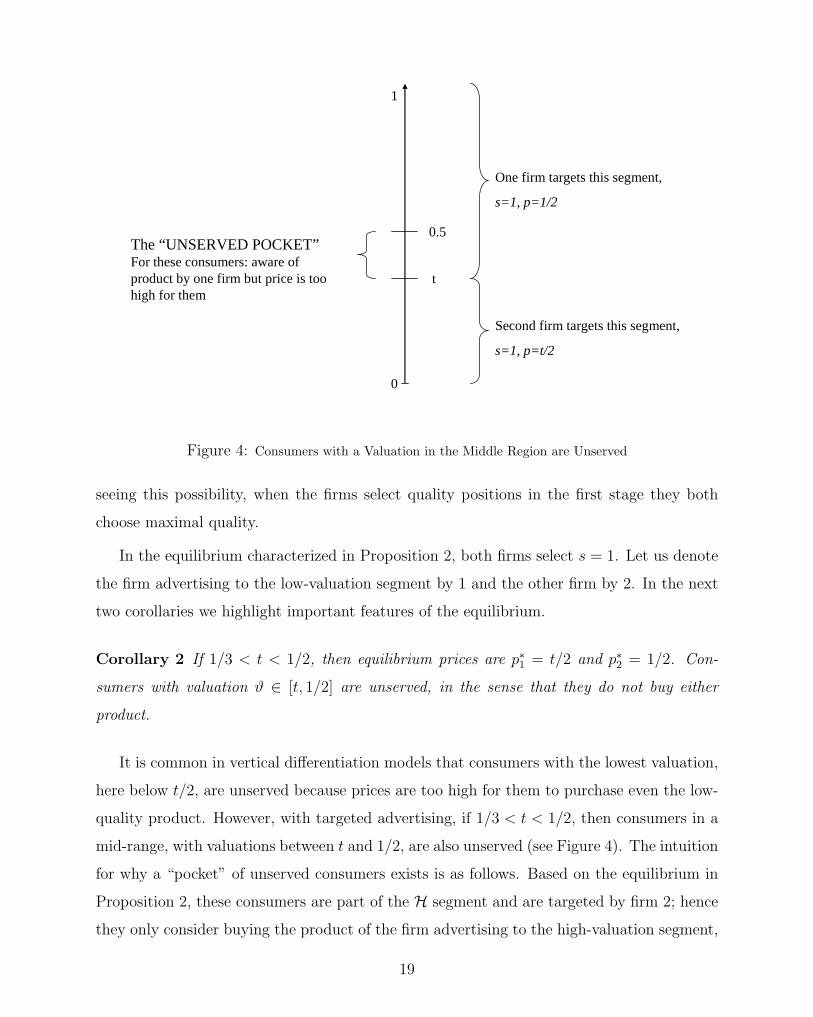
Proposition 2 If 1/3 ≤ t ≤ 4/5 then the only equilibria of the game are represented by

those sets of strategies where si = sj = 1, Si = L, Sj = H, pi = t/2 and pj = max(t, 1/2).

Firms’ profits are Πi = t2/4 and Πj = 1/4 for t < 1/2 and Πj = t(1− t) for t ≥ 1/2.

The intuition behind this result is that in the advertising stage firms prefer to choose

disjunct segments, thereby “dividing” the market. Doing so allows them to act as de facto

monopolists in their chosen segments and avoid price competition in the final stage. Fore-

8Thus, we examine the realistic case where firms cannot identify each and every consumer and knowtheir exact willingness to pay for quality. Through market research and experience, though, the firms canuse proxy variables that provide a relatively accurate split of consumers as those having a greater vs. lowervaluation for product quality in the category.

18

0

Targeted Advertising

1

t

One firm targets this segment,

s=1, p=1/2

Second firm targets this segment,

s=1, p=t/2

Distribution of Valuation for Quality

0.5The “UNSERVED POCKET”For these consumers: aware of product by one firm but price is too high for them

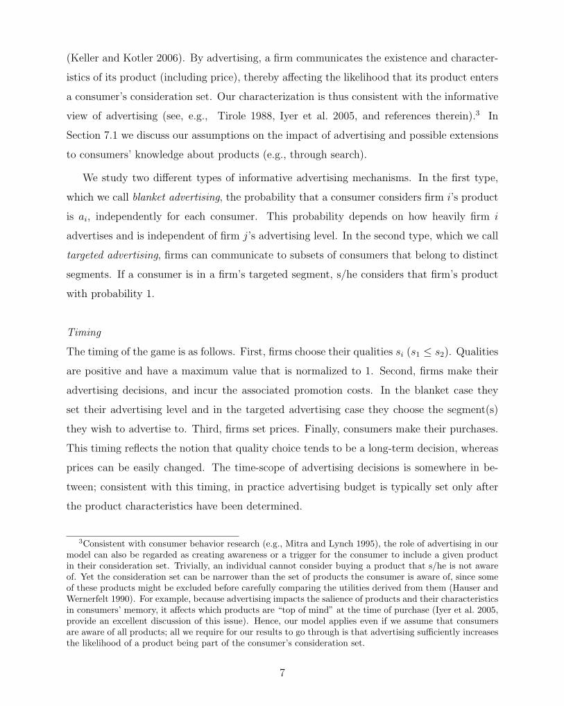
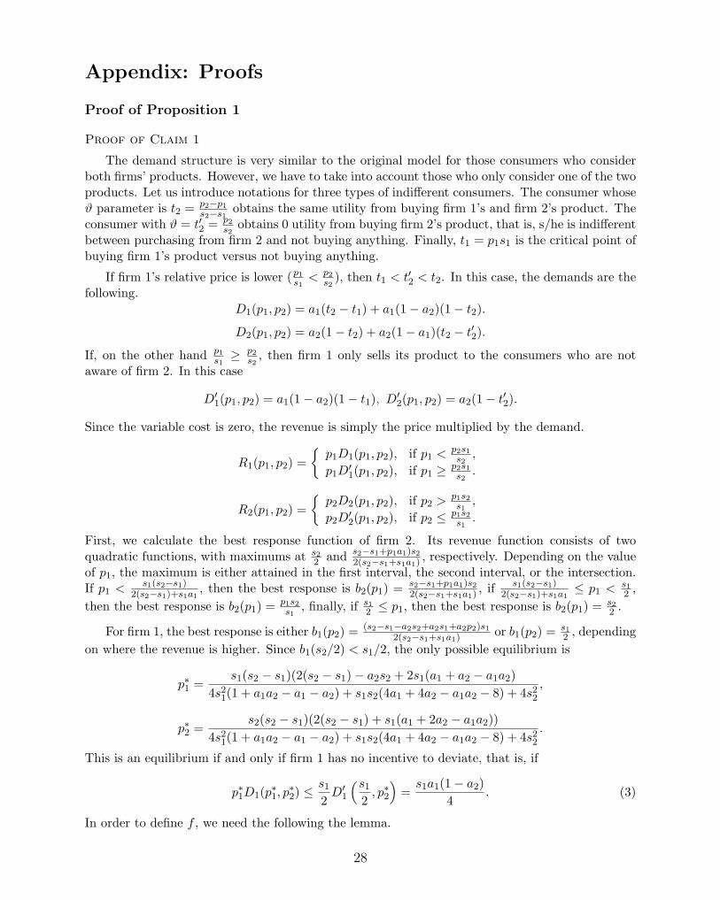
Figure 4: Consumers with a Valuation in the Middle Region are Unserved

seeing this possibility, when the firms select quality positions in the first stage they both

choose maximal quality.

In the equilibrium characterized in Proposition 2, both firms select s = 1. Let us denote

the firm advertising to the low-valuation segment by 1 and the other firm by 2. In the next

two corollaries we highlight important features of the equilibrium.

Corollary 2 If 1/3 < t < 1/2, then equilibrium prices are p∗1 = t/2 and p∗2 = 1/2. Con-

sumers with valuation ϑ ∈ [t, 1/2] are unserved, in the sense that they do not buy either

product.

It is common in vertical differentiation models that consumers with the lowest valuation,

here below t/2, are unserved because prices are too high for them to purchase even the low-

quality product. However, with targeted advertising, if 1/3 < t < 1/2, then consumers in a

mid-range, with valuations between t and 1/2, are also unserved (see Figure 4). The intuition

for why a “pocket” of unserved consumers exists is as follows. Based on the equilibrium in

Proposition 2, these consumers are part of the H segment and are targeted by firm 2; hence

they only consider buying the product of the firm advertising to the high-valuation segment,

19

and this firm charges a price of p∗2 = 1/2. But since for them ϑ − 1/2 < 0, i.e., the price is

above their maximum willingness to pay, they do not purchase any product.

The next corollary summarizes how the demand changes as a function of t, the size of

the low-valuation segment.

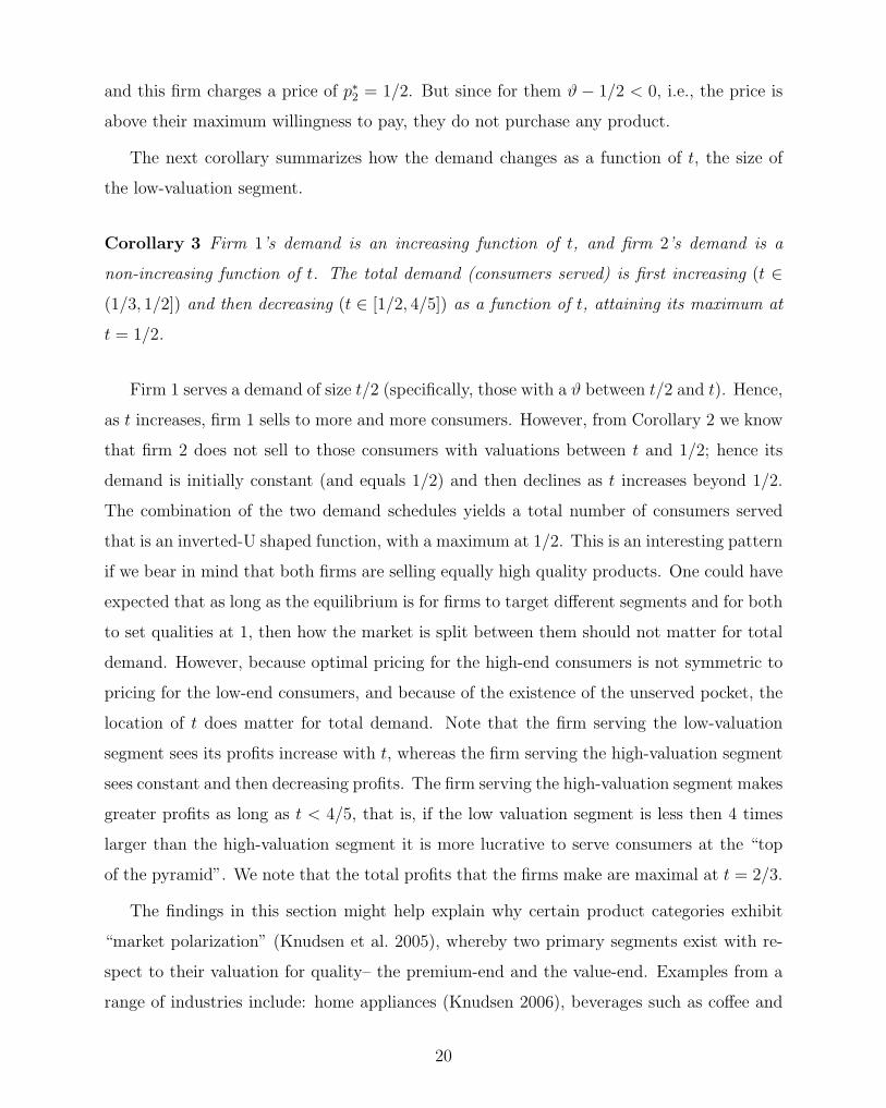
Corollary 3 Firm 1’s demand is an increasing function of t, and firm 2’s demand is a

non-increasing function of t. The total demand (consumers served) is first increasing (t ∈

(1/3, 1/2]) and then decreasing (t ∈ [1/2, 4/5]) as a function of t, attaining its maximum at

t = 1/2.

Firm 1 serves a demand of size t/2 (specifically, those with a ϑ between t/2 and t). Hence,

as t increases, firm 1 sells to more and more consumers. However, from Corollary 2 we know

that firm 2 does not sell to those consumers with valuations between t and 1/2; hence its

demand is initially constant (and equals 1/2) and then declines as t increases beyond 1/2.

The combination of the two demand schedules yields a total number of consumers served

that is an inverted-U shaped function, with a maximum at 1/2. This is an interesting pattern

if we bear in mind that both firms are selling equally high quality products. One could have

expected that as long as the equilibrium is for firms to target different segments and for both

to set qualities at 1, then how the market is split between them should not matter for total

demand. However, because optimal pricing for the high-end consumers is not symmetric to

pricing for the low-end consumers, and because of the existence of the unserved pocket, the

location of t does matter for total demand. Note that the firm serving the low-valuation

segment sees its profits increase with t, whereas the firm serving the high-valuation segment

sees constant and then decreasing profits. The firm serving the high-valuation segment makes

greater profits as long as t < 4/5, that is, if the low valuation segment is less then 4 times

larger than the high-valuation segment it is more lucrative to serve consumers at the “top

of the pyramid”. We note that the total profits that the firms make are maximal at t = 2/3.

The findings in this section might help explain why certain product categories exhibit

“market polarization” (Knudsen et al. 2005), whereby two primary segments exist with re-

spect to their valuation for quality– the premium-end and the value-end. Examples from a

range of industries include: home appliances (Knudsen 2006), beverages such as coffee and

20

vodka (Deshpande 2001), and network storage hardware (Ofek and Hamid 2005). In these

cases, we typically find that each firm focuses on a distinct segment and targets its commu-

nications and distribution to that segment. Moreover, and consistent with our findings, even

though in reality quality and production costs can be similar across offerings, the prices of

products targeted at value-oriented customers are typically much lower than those targeted

at premium-oriented customers.9 Mounting evidence also suggests that serving consumers

with intermediate willingness to pay values is not beneficial. Indeed, recent management

consulting practice calls on firms to “escape the middle-market trap” (Knudsen 2006).

We have focused in this section on the case where the low willingness to pay segment

comprises at least 33% of the market and the high willingness to pay segment at least 20%.

This ensures that these segments are advertised to in equilibrium.10 We believe this is the

relevant case to analyze because for many real world settings, targeting criteria are only

meaningful if they result in segments with a sufficient proportion of consumers. That said,

we now explain what happens when t does not satisfy the conditions in Proposition 2. If

t < 1/3, then the low willingness to pay interval (L) might be too small for either firm to

want to advertise to it, and both may end up advertising only to consumers in the high

willingness to pay interval (H). In this case, if one firm sets s2 = 1, then the rival will set

a quality level higher than s1 = 4/7 because its market size is limited by the lower bound

of the interval. On the other hand, if t is close to 1 neither firm can afford to forgo the

low-valuation segment, and both firms will include it in their target market (and advertise

to it). In this region, it is complex to characterize the full set of possible equilibria, but it

should be clear that as t approaches 1 the model effectively reduces to Shaked and Sutton

(1982); one firm selects the maximal quality of s = 1 and its rival sets s = 4/7.

9In the case of home appliances, outsourcing parts or complete production has resulted in similar variablecosts, yet products aimed at the premium end are 2-3 times more expensive. In the vodka market, blindtaste tests consistently reveal the top brands as roughly equally rated and their ingredients and processesare similar. However, the average price of a 750ml bottle of Smirnoff is about $13 while that of GreyGoose is about $32. The former vodka is primarily targeted at casual consumption (low willingness to payconsumers), while the latter for heavy vodka drinkers. In the market for SAN storage devices, firms wereable to target separate segments despite selling equally advanced products (the technology used was similar,the only difference was the configuration of the device; McData sold to high-end data centers and Brocadesold to customers with less data-intensive applications).

10It is not surprising that the lower bound (0.33) is larger than the upper bound (0.20). The margin on thelow willingness to pay consumers is small hence this segment (L) has to be big enough in size to be targeted,while the margin on the highest willingness to pay consumers can compensate for a smaller segment size(H).

21

6 Persuasive Advertising

In this section, instead of focusing on the informative features of advertising as before, we

examine the case of persuasive advertising. We assume that all consumers are aware of the

products available but the quality they perceive each of the offerings to possess is affected

by the advertising they are exposed to. Thus, in determining which product to buy, what

matters for the consumer is the net perceived utility. There is evidence that in certain cases

advertising affects buying decisions in this way. For example, in an empirical study Moorthy

and Zhao (2000) find (across ten product categories) that advertising effort (spending) has

a positive effect on perceived quality. Based on this phenomenon, we modify the model in

the following way.11

Let si denote the real (or objective) quality of the product offered by firm i. As before,

let ai denote firm i’s advertising impact. We assume that 0 ≤ ai ≤ 1 and that the perceived

quality of product i is aisi. This simple formulation captures the fact that by advertising

more the firm can raise its product’s perceived quality. However, the real quality forms an

upper limit to the perceived quality.12 Aside from the way advertising impacts demand, the

setup of the game is equivalent to that of the blanket advertising model presented in Section

4. Firms first choose qualities, then advertising efforts and, finally, prices (decisions in each

stage are simultaneous).

As a first step, let us examine a very simple case in which advertising is costless. Despite

the oversimplifying assumption, the analysis sheds light on how firms differentiate in qualities

when they can use advertising to change product perceptions.

Claim 3 The game has infinitely many sub-game perfect equilibria, where sj = 1 and si can

take any value between 4/7 and 1. Furthermore, in every equilibrium aisi = (4/7)ajsj.

Interestingly, the degree of objective quality differentiation is less than or equal to the

ratio s1/s2 = 4/7, which is the degree of differentiation in the basic model (with no persuasive

11Colombo and Lambertini (2003) study persuasive advertising in a dynamic setting with endogenousquality levels. An important difference is that we examine how advertising changes consumers’ valuationsof the product, whereas they assume a reduced functional form for the effect of advertising on demand.Furthermore, these authors do not consider informative advertising.

12This formulation produces equivalent results as a formulation in which the upper limit is any linearfunction of the real quality.

22

advertising and full awareness). However, note that firms will use persuasive advertising

to increase the perceived differentiation so that, from consumers’ perspective, the ratio of

perceived qualities is always 4/7.

In order to relax the assumption of costless advertising, let us assume that advertising

effort is a discrete variable (as in Section 4). Firms can choose between ai = aL and ai = aH ,

where 0 ≤ aL < aH ≤ 1. Let cL and cH denote the costs associated with the two advertising

levels, with cL sufficiently low so that both firms advertise. Again, let c = cH − cL.

Proposition 3 There exist values c and c (0 < c < c), such that we get the following

sub-game perfect equilibria

1. If c ≤ c, then si = 4/7, sj = 1 and the advertising equilibrium is (L,L).

2. If c ≤ c < c, then si = (4/7)(aH/aL), sj = 1 and the advertising equilibrium is (L,H).

3. If 0 < c < c, then si = 4/7, sj = 1 and the advertising equilibrium is (H,H),

Intuitively, if the extra cost of advertising heavily is sufficiently high, then both firms choose

the light level. If the cost difference is in the middle range, one firm chooses to advertise

heavily and the other lightly. Lastly, if the cost differential is low, both firms find it beneficial

to advertise heavily.

Turning now to explaining the equilibrium quality decisions, note that in the two extreme

advertising cost regions the objective qualities are as in the original Shaked and Sutton (1982)

model (s1/s2 = 4/7). Given that both firms either advertise heavily or lightly, the degree of

perceived differentiation is the same as without advertising. However, in the middle range

we find the same phenomenon as in the simple case of Claim 3. The objective quality ratio

s1/s2 is higher than 4/7, corresponding to a smaller degree of objective differentiation, which

is then counterbalanced by the difference in advertising efforts; leading to a perceived quality

ratio of exactly 4/7 = (s1a1)/(s2a2).

To summarize, with persuasive advertising the degree of perceived quality differentiation

is always the same and corresponds to the case where advertising has no persuasive effect

(and with all consumers informed). That said, in choosing its objective quality a firm has

to be mindful of the advertising levels that will be chosen. In particular, if a firm faces a

23

rival that selects maximal quality and the equilibrium advertising levels are expected to be

asymmetric, then the firm should select a relatively high objective quality to overcome the

fact that it will only advertise lightly.

7 Conclusion

In this paper, our goal has been to study the interaction between endogenous quality choice

and the desire to advertise products to consumers. We developed a model in which firms

choose product quality in a first stage, their advertising strategy in a second stage, and prices

in the last stage. We explored two forms of informative advertising – blanket and targeted.

In an extension, we also examined the implications of persuasive advertising, which serves

to affect consumers’ perception of product quality.

In the case of blanket advertising, we showed that firms can be better off under light levels

of advertising because this allows them to choose higher product quality positions yet avoid

fierce price competition. Moreover, the equilibria of the game depend on the cost-efficiency of

advertising. When advertising is relatively ineffective, differentiation is relatively modest and

both firms advertise at a light level. When, at the other extreme, advertising is very effective,

one firm chooses maximal quality and expends heavily on advertising. The rival now prefers

to differentiate with a much lower quality product and expend lightly on advertising. The

smallest degree of quality differentiation occurs in a mid range of advertising effectiveness.

By positioning its product close by, a firm prevents its high-quality rival from switching

to a heavy level of advertising expenditure. Moreover, in this range as ad effectiveness

increases the firm will select an even higher quality position. This results in products that

are minimally differentiated and, in turn, prices decline.

Under targeted advertising, our main result was that each firm advertises to a different

segment. Thus, firms do not directly compete in the pricing stage and can both choose

equally high quality products– that is, their offerings are entirely undifferentiated. Interest-

ingly, due to the relatively high prices firms charge, there exist conditions such that a set

of consumers with moderate valuation for quality are unserved by the firm that advertises

to them– even though consumers in a different segment with lower willingness to pay are

served by the rival firm. We also showed that the total number of consumers served is an

24

inverted-U function of the low-valuation segment size.

In an extension, we studied the role of persuasive advertising. Our main result there is

that firms may differentiate less in objective qualities, but the asymmetry in advertising levels

counterbalances this effect; leading to the same degree of perceived quality differentiation as

when no persuasive advertising is possible (and all consumers are fully informed about the

products available).

These findings have several important managerial implications. First, they suggest that

the conventional wisdom whereby a firm should seek a high degree of product differentiation

from its rival to avoid head-to-head price competition is qualified, and depends on whether or

not there is a role for informative advertising that generates awareness or impacts consumer

consideration of the products offered. It further matters what kind of communication vehicles

the firms can use to reach consumers. If firms cannot identify consumers through any

targeting criterion and use blanket advertising (also referred to as national advertising), the

degree of quality differentiation depends on how effective advertising is. Most managerial

treatments of advertising classify media based on their impact on consumers and their cost

(see, e.g., Thomas et al. 2000, exhibit 14.17). Our results thus tell managers how the specific

characteristics of advertising vehicles in their market should affect the quality of products

they choose to offer. By contrast, when firms can target distinct segments our findings

suggest that no differentiation in quality may actually work best, provided the firms can

“stay out of each other’s turf”. Importantly, our analysis reveals that a firm need not feel

forced to lower price so as to serve all the consumers who have been targeted; the firm

may wish to ignore consumers that have moderate willingness to pay, even though low-end

consumers are being served by the rival firm. In other words, “avoiding the middle segment”

may be the best course of action.

Second, it is important to bear in mind that while industry funded R&D is approximately

$240 billion per year in the U.S. (NSF 2008), companies spend comparable amounts on

advertising (as noted in the Introduction, about $155 billion in 2006); and this holds for

many high-tech firms as well.13 Hence, when setting new product strategy, which is often

aimed at improving the quality of existing products (e.g., higher levels of key attributes),

13For instance, in 2006 Intel Corp. spent $5.8 billion on R&D compared to $6.1 billion on marketing(source: Intel 2006 10k report).

25

to ensure the best possible commercial outcome it is crucial to take into account how the

new products will be advertised to potential customers. In their seminal work surveying

managers on how firms appropriate returns from R&D investments given competitors, Levin

et al. (1987) found that marketing and sales effort were cited as the primary vehicle (over such

means as patents and trade secrets). This clearly suggests that managers need to understand

the strategic implications of communication strategy on the products they choose to develop

vis-a-vis the products their rivals are expected to develop.

7.1 Limitations and Future Research

Although our study encompasses three different types of advertising and we have justi-

fied many of our assumptions, we acknowledge several limitations. First, we analyzed the

advertising models separately. One could imagine a general a model where advertising is

informative and persuasive at the same time (or that firms need to choose the levels of both

types of advertising). Also, by combining the first two models presented (in Sections 4 and

5), we would get a general setting in which advertising can be targeted but its impact within

the segment may not be perfect, resulting in two decision variables: which segment(s) to

target and how aggressively to try and reach consumers in the chosen segment(s).

Second, in Sections 4 and 5 we assumed that the only way for consumers to become

informed was through advertising. This allowed us to focus on advertising’s role in affecting

whether consumers consider a given product and, in turn, firms’ strategic incentives to

expend on advertising and their quality choices. In reality, of course, consumers have other

ways to become informed about the products available, e.g., through search (prior to visiting

the store or at the store).14 Assuming that a given consumer has a positive probability of

becoming informed about the firm’s product even without receiving an ad for it would not

change our model findings, as long as this probability is not too high. In this case, we

would interpret advertising in our model as increasing this probability by ai. Our results

would also hold if consumer search costs are sufficiently high so that not all consumers

have an incentive to become fully informed. However, if consumer search costs are only

moderate, uninformed consumers may have a greater incentive to search than informed

14Note that sales assistance at the store can be regarded as part of a firm’s promotion strategy (as a firmcan offer more or less retail incentives; choose the retailers it provides the product to, etc.).

26

consumers, which could impact our findings. We leave for future research the investigation

of how combining informative advertising and consumer search affects endogenous quality

positions.

Third, we have employed very stylized assumptions on costs. In order to simplify the

presentation and analysis, we assumed that products are produced at a zero variable cost

(that is not a function of quality). In this way we were able to focus on the strategic forces

that drive the degree of quality differentiation and the interaction with advertising. It is also

a reasonable assumption in many product categories where variable costs are either negligible,

e.g., digital goods or drugs, or only weakly related to quality positions. Future research could

examine the implications of including variable costs that are a function of product quality.

It is conceivable, for example, that if variable costs are a convex function of quality that the

high-quality firm earns a smaller margin on its product than the lower-quality rival does,

and hence has less incentive to advertise heavily than in the model presented here; this could

affect the nature of the results.

Fourth, in this paper we have focused on consumer heterogeneity in willingness to pay

for quality. This allowed us to examine how vertical differentiation is impacted by the need

to inform consumers about product offerings. In reality, of course, consumers may also

exhibit heterogeneity in horizontal tastes (e.g., some consumers preferring contemporary

furniture designs while others preferring old-fashioned designs). It is conceivable that firms’

choice of product positioning along a horizontal continuum may be impacted by the need

to advertise to make consumers aware of their offerings, and there may be an even greater

role for persuasive advertising in this case. The interaction between product location and

advertising with horizontal heterogeneity can be fruitful ground for future research.

27

Appendix: Proofs

Proof of Proposition 1

Proof of Claim 1

The demand structure is very similar to the original model for those consumers who considerboth firms’ products. However, we have to take into account those who only consider one of the twoproducts. Let us introduce notations for three types of indifferent consumers. The consumer whoseϑ parameter is t2 = p2−p1

s2−s1obtains the same utility from buying firm 1’s and firm 2’s product. The

consumer with ϑ = t′2 = p2

s2obtains 0 utility from buying firm 2’s product, that is, s/he is indifferent

between purchasing from firm 2 and not buying anything. Finally, t1 = p1s1 is the critical point ofbuying firm 1’s product versus not buying anything.

If firm 1’s relative price is lower (p1

s1< p2

s2), then t1 < t′2 < t2. In this case, the demands are the

following.D1(p1, p2) = a1(t2 − t1) + a1(1− a2)(1− t2).

D2(p1, p2) = a2(1− t2) + a2(1− a1)(t2 − t′2).

If, on the other hand p1

s1≥ p2

s2, then firm 1 only sells its product to the consumers who are not

aware of firm 2. In this case

D′1(p1, p2) = a1(1− a2)(1− t1), D′2(p1, p2) = a2(1− t′2).

Since the variable cost is zero, the revenue is simply the price multiplied by the demand.

R1(p1, p2) ={

p1D1(p1, p2), if p1 < p2s1

s2,

p1D′1(p1, p2), if p1 ≥ p2s1

s2.

R2(p1, p2) ={

p2D2(p1, p2), if p2 > p1s2

s1,

p2D′2(p1, p2), if p2 ≤ p1s2

s1.

First, we calculate the best response function of firm 2. Its revenue function consists of twoquadratic functions, with maximums at s2

2 and s2−s1+p1a1)s2

2(s2−s1+s1a1) , respectively. Depending on the valueof p1, the maximum is either attained in the first interval, the second interval, or the intersection.If p1 < s1(s2−s1)

2(s2−s1)+s1a1, then the best response is b2(p1) = s2−s1+p1a1)s2

2(s2−s1+s1a1) , if s1(s2−s1)2(s2−s1)+s1a1

≤ p1 < s12 ,

then the best response is b2(p1) = p1s2

s1, finally, if s1

2 ≤ p1, then the best response is b2(p1) = s22 .

For firm 1, the best response is either b1(p2) = (s2−s1−a2s2+a2s1+a2p2)s1

2(s2−s1+s1a1) or b1(p2) = s12 , depending

on where the revenue is higher. Since b1(s2/2) < s1/2, the only possible equilibrium is

p∗1 =s1(s2 − s1)(2(s2 − s1)− a2s2 + 2s1(a1 + a2 − a1a2)

4s21(1 + a1a2 − a1 − a2) + s1s2(4a1 + 4a2 − a1a2 − 8) + 4s2

2

,

p∗2 =s2(s2 − s1)(2(s2 − s1) + s1(a1 + 2a2 − a1a2))

4s21(1 + a1a2 − a1 − a2) + s1s2(4a1 + 4a2 − a1a2 − 8) + 4s2

2

.

This is an equilibrium if and only if firm 1 has no incentive to deviate, that is, if

p∗1D1(p∗1, p∗2) ≤ s1

2D′1

(s1

2, p∗2

)=

s1a1(1− a2)4

. (3)

In order to define f , we need the following the lemma.

28

Lemma 1 R(s1) = p∗1D1(p∗1, p∗2) is a concave function of s1 for 0 ≤ s1 ≤ s2, R(0) = R(s2) = 0

and R′(0) > a1(1− a2)/4 for a1, a2 > 0.

Proof: We can assume without loss of generality that s2 = 1. Then

R(s1) =(1− s1)(1− s1 + a2s1)(−2a2s1 + 2s1 − 2s1a1 + 2a1s1a2 − 2 + a2)2a1s1

(−a1s1a2 + 4− 8s1 + 4s1a1 + 4s21 − 4s2

1a1 + 4a2s1 − 4a2s21 + 4a2s2

1a1)2,

which is concave for 0 ≤ s1 ≤ 1, and

R′(0) =(2− a2)2a1

16>

a1(1− a2)4

for a1, a2 > 0

Now, let f(a1, a2) be the solution of the equation

p∗1D1(p∗1, p∗2) =

s1a1(1− a2)4

,

with respect to s1, setting s2 to 1. Since the left hand side is a concave and the right hand size islinear function of s1, the solution is unique in the interval 0 ≤ s1 ≤ 1, and according to the lemma0 < f < 1. Since s1 only satisfies (3) if and only if s1 ≤ f(a1, a2), we have proved parts 1 and 2.

Then f(a1, 1) = 1 for any 0 < a1 ≤ 1 also obviously follows from the lemma. In order to provethat f(a, a) is increasing in a, we have to examine the function R(s1) more carefully. One can checkthat

R(s1)− s1a(1− a)4

is increasing in a if 1/2 ≤ a = a1 = a2 for any 0 ≤ s1 ≤ 1. Since R(s1) is concave and R(0) = 0this proves that f(a, a) is increasing for a ≥ 1/2.

If s1 = s2 and both advertising probabilities are positive, then there is always a positive massof consumers, who are aware of both products. Thus, in a symmetric equilibrium, both prices haveto be zero as a consequence of the Bertrand-type competition. On the other hand, asymmetricequilibria do not exist, since any of the firms would be better off by setting a price of s1/2 = s2/2.

Proof of Claim 2

Let G1L(s1) = R1

HL(s1)−R1LL(s1), G1

H(s1) = R1HH(s1)−R1

LH(s1) G2L(s1) = R2

LH(s1)−R2LL(s1),

G2H(s1) = R1

HH(s1)−R2HL(s1) denote the gains of setting advertising to heavy instead of light. In

order to determine a∗, we need the following observations, that can be proved by basic algebraiccalculations.

Observation 1 Let G(q) denote the derivative (G1H(1)−G2

H(1))′ as a function of q for 0 ≤ q ≤ 1.Then G(q) is an increasing function, and G(q) = 0 has a solution in the interval 0 ≤ q ≤ 1.

Let a∗ be the solution of G(q) = 0, which is a∗ ≈ 0.7032. Note that since a∗ > 1/2, our assumptionthat aL > a∗ is consistent with numerous empirical studies showing that the advertising responsefunction is concave (Lilien and Rangaswamy 2004).

Observation 2 If aL > a∗, then G1L(s1) < G2

L(s1) and G1H(s1) < G2

H(s1) for 0 < s1 < 1.

29

Now let us examine when the different types of equilibria are possible.

• (L,L)If firm 1 chooses L, then firm 2’s best response to this is L if and only if c ≥ G2

L(s1). Firm1’s best response to this is L if and only if c ≥ G1

L(s1). Since G1L(s1) < G2

L(s1), this type ofequilibrium emerges only if c ≥ G2

L(s1). For its existence we also need that an equilibriumin the last stage exist, that is, s1 ≤ f(aL, aL), otherwise no equilibrium exists.

• (L,H)If firm 1 chooses L, then firm 2’s best response to this is H if and only if c ≤ G2

L(s1). Firm 1’sbest response to this is L if and only if c ≥ G1

H(s1). Since in this case the pricing equilibriumalways exists (f(q,1)=1), this type of equilibrium emerges if and only if G1

H(s1) ≤ c ≤ G2L(s1).

• (H,H)If firm 1 chooses H, then firm 2’s best response to this is H if and only if c ≤ G2

H(s1). Firm1’s best response to this is H if and only if c ≤ G1

H(s1). Since G1H(s1) < G2

H(s1) and thepricing equilibrium always exists, this type of equilibrium emerges if and only if c ≥ G1

H(s1).This completes the proof of the claim

In order to complete the proof we need the following observations, that can be proved by basicalgebraic calculations.

Observation 3 G2L(s1) is decreasing for 0 ≤ s1 ≤ 1.

Observation 4 We have R2LH(s1) < R2

LL for 0 < s1 < 1.

Observation 5 We have max{0≤s1≤1}R1LH(s1) = max{0≤s1≤1}R

1HH(s1).

Let s = arg max(R1LL(s1)) and s = arg max(R1

LH(s1)) and let c = G2L(s) and c = G2

L(f(aL, aL)).Consequently, e = 1−aL

G2L(s)

and e = 1−aL

G2L(f(aL,aL))

.

We now start analyzing the equilibria at the quality choice stage. Let us first examine firm 1’sbest response quality choice to s2 = 1.

• If cM > c > c, that is, if eM < e < e, then depending on s1 the advertising equilibrium iseither (L, H) or (L, L). Let s′ = (G2

L)−1(c) denote the critical value for (L, L) to realize.Therefore, firm 1 maximizes R1

LH in the interval 0 ≤ s1 ≤ s′ and R2LL in the interval

s′ ≤ s1 ≤ 1. According to Observation 4, the maximum of R2LL is greater than the maximum

of R1LH . On the other hand, it follows from the definition of c that R2

LL attains its maximumin the interval s′ ≤ s1 ≤ 1, hence firm 1’s best response is s and the advertising strategies are(L, L). Note that according to the definition of c, the pricing equilibrium exist in this case.

• If c > c > c, that is, if e < e < e, then firm 1 still maximizes R1LH in the interval 0 ≤ s1 ≤ s′

and R2LL in the interval s′ ≤ s1 ≤ 1. However, in this case, R2

LL() does not attain itsmaximum in the interval s′ ≤ s1 ≤ 1. On the other hand, R2

LL(s′) ≥ max{0≤s1≤1}R2LH(s1),

therefore, the best response of firm 1 is s′ = (G2L)−1(c) and the advertising strategies are

(L, L). Note that according to the definition of c, the advertising equilibrium still exist inthis case.

30

• If c > c ≥ 0, that is, if e > e, let s′′ and s′′′ denote the two solutions of G1H(s1) = c, if

they exist. Then firm 1 maximizes R1LH in the interval 0 ≤ s1 ≤ s′, except for the interval

s′′ ≤ s1 ≤ s′′′, where it maximizes R1HH − c, if s′′ and s′′′ exist, that is, if c ≤ max G1

H(s1).Since max{0≤s1≤1}R

1LH(s1) = max{0≤s1≤1}R

1HH(s1), firm 1’s best response is always s and

the advertising strategies are (L, H).

In order to show that the above strategies consist equilibria, we have to make sure that firm 2’sresponse to firm 1’s actual action is s2 = 1. Note that firm 2’s profit functions R2

LL(s2), R2LH(s2)

and R2HH(s2) are all increasing if we fix s1 at a certain level. Thus, the only incentive for firm 2 to

not to choose s2 = 1 would be to change the advertising equilibrium and increase its payoff troughthat. This is, however, not possible as the only change that it could attain by decreasing s2 from1 is to change an (L, H) equilibrium to an (L, L) which is obviously not profitable. Thus, we haveconfirmed that all the above described strategies are equilibria.

We have to show that no other equilibrium exists, that is, that s2 is always 1 in equilibrium.Let us assume that an equilibrium exists with s∗2 < 1. The advertising equilibria and the bestresponse of firm 1 can be calculated the same way as for s2 = 1, except that the s1 values have tomultiplied by s∗2. As mentioned before, for a fixed advertising equilibrium and a fixed s1, the profitof firm 2 is strictly increasing in s2. Thus, the only way firm 2 has no incentive to increase s2 isif that would change the advertising equilibrium and decrease profits. However, the above casesshow that the only possibility to such a change would be from (L, L) to (L, H), but that does notdecrease firm 2’s profit. This completes the proof of the proposition.

Proof of Proposition 2

First, we examine the pricing stage of the game given the quality levels and the advertising segments.

1. If the two segments are distinct, that is, if S1 ∩ S2 = ∅, then there is no price competitionbetween the firms. They both maximize their income in their own segment. For the firmchoosing the high interval (Si = H), the optimal price is p∗i = max(si/2, sit). For the firmchoosing the low interval (Sj = L), the optimal price is p∗i = sjt/2.

2. If both firms choose both intervals, that is , if S1 = S2 = L ∪ H, then there is full pricecompetition and the pricing equilibria are the same as in the Shaked and Sutton model. Wehave also covered this case in Claim 1 (substituting a1 = a2 = 1): if s1 = s2, then prices godown to zero, whereas if s1 < s2, then

p∗1 =s1(s2 − s1)

4s2 − s1, p∗2 =

2s2(s2 − s1)4s2 − s1

,

where the indifferent consumer has a ϑ of t∗2 = p∗2−p∗1s2−s1

= 2s2−s14s2−s1

.

3. If the firms choose the same intervals, for example S1 = S2 = H, then in case of s1 = s2,equilibrium prices are zero. If s1 < s2, then depending on t two equilibria are possible. Ifs2−s14s2−s1

≤ t ≤ s2−s12s2+s1

, then

p∗1 = ts1, p∗2 =s2 − s1 + ts1

2.

If t ≥ s2−s12s2+s1

, then

p∗1 =(s2 − s1)(1− 2t)

3,

31

p∗2 =(s2 − s1)(2− t)

3.

4. If S1 = S2 = L, then in case of s1 = s2, equilibrium prices are zero. If s1 < s2, then thegame is equivalent to Case 2, but we have to normalize the top of the interval to 1, that is,

p∗1 = ts1(s2 − s1)

4s2 − s1, p∗2 = t

2s2(s2 − s1)4s2 − s1

,

5. If S1 = L and S2 = L∪H, then in case of s1 = s2 equilibrium prices are zero. If s1 < s2, thenthe price competition is limited to consumers below t. That is, firm 1 only has an incentiveto decrease prices until the position of the indifferent consumer (t2 = p2−p1

s2−s1) reaches either

t or t∗2. That is, in case of t > t∗2, the equilibrium prices are the same as in Case 2. On theother hand, if t ≤ t∗2 then p∗1 = s1t/2 and p∗2 = max(s2/2, s2t).

6. If S1 = L ∪ H and S2 = H, then in case of s1 = s2 equilibrium prices are zero. If s1 < s2,the price competition is limited to consumers above t. That is, firm 2 only has an incentiveto decrease prices until the position of the indifferent consumer (t2 = p2−p1

s2−s1) reaches either

t or t∗2. That is, in case of t < t∗2, the equilibrium prices are the same as in Case 2. On theother hand, if t ≥ t∗2 then p∗1 = s1t/2 and p∗2 = max(s2/2, s2t).

7. If S1 = H and S2 = L ∪ H, then in case of s1 = s2, equilibrium prices are zero. If s1 < s2,then

p∗1 =(s2 − s1)(2ts1 + s2 − 3ts2)

7s2 − 4s1, p∗2 =

(s2 − s1)(t + 2)s2

7s2 − 4s1

form an equilibrium, since t > 1/3 is assumed.

8. If S1 = L ∪ H and S2 = L, then in case of s1 = s2 equilibrium prices are zero. If s1 < s2,then

p∗1 =s1(s2 − s1)(2− t)

4s2 − s1, p∗2 =

(s2 − s1)(2ts2 − ts1 + s1)4s2 − s1

.

9. If either firm chooses not to advertise then the other firm is a monopolist in its segment,setting the price to max(six, siy/2) if the segment is the [x, y] interval.

Let us now turn our attention to the advertising stage of the game and determine which segmentsfirms choose to advertise to. Let us examine the different types of possible equilibria. An equilibriumis described by a pair (S1, S2), where the first set denotes the segment chosen by firm 1 and thesecond set denotes the segment chosen by firm 2. First we fix s1 < s2 and determine which typesof equilibria are possible if 4/5 > t ≥ 1/3. Note that we do not consider cases where a firm doesnot advertise.

• (L,H) : In this case, R1 = s1t2/4, R2 = s2/4 if t < 1/2 and R1 = s1t

2/4, R2 = s2t(1 − t)if t ≥ 1/2. In order to check when this constitutes and equilibrium we have to check threecases. First, if t ≥ 1/2, then firm 1 has no incentive to deviate since it cannot reach consumersabove t∗2 = 2s2−s−1

4s2−s1≤ 1/2. Firm 2 is better off by choosing S2 = L ∪H if and only if

4s22(s2 − s1)

(4s2 − s1)2− s2t(1− t) > cL = tcU . (4)

32

If 1/2 > t > t∗2, then the condition becomes

4s22(s2 − s1)

(4s2 − s1)2− s2

4> cL = tcU . (5)

Finally, if t∗2 ≥ t, then firm 2 has no incentive to deviate, however firm 1 does if and only if

s1s2(s2 − s1)(4s2 − s1)2

− s1t2/4 > cH = (1− t)cU . (6)

• (L ∪ H,H) : In this case, firm 2 has no incentive to deviate. However, firm 1 is better offsetting S1 = L if t ≥ t∗2. If t < t∗2, then firm 1 deviates if and only if (6) does not hold.

• (L,L ∪ H) : In this case, firm 1 has no incentive to deviate. However, firm 2 is better offsetting S1 = H, if t ≤ t∗2. If t > t∗2, then firm 2 will deviate if and only if (4) and (5) do nothold in the cases of t ≥ 1/2 and 1/2 > t > t∗2, respectively.

In the following cases one of the firms always has an incentive to deviate, thus, they do notconstitute equilibria. We assume that firms make positive profits, otherwise it would be profitablefor them to not advertise at all.

• (L ∪ H,L ∪ H) : In this case, either firm 1 or firm 2 has an incentive to deviate. If t ≤ t∗2 =2s2−s14s2−s1

, then consumers below t∗2 will not buy from firm 2, therefore firm 2 is better off settingS2 = H. On the other hand, if t ≥ t∗2, then firm 1 is better off setting S1 = L.

• (L,L) : In this case, firm 2’s revenues are t24s2

2(s2−s1)4s2−s1

. If firm 2 chooses S2 = L ∪H instead,

then its revenues become at least 4s22(s2−s1)

(4s2−s1)2which is at least 1/t2 times more. Since costs are

only 1/t times more, firm 2 has incentive to deviate.

• (H,H): If t ≥ s2−s12s2+s1

, then firm 1 has an incentive to choose S1 = L, because then it makess1t

2/4− tcU instead of (2t− 1)2(s2− s1)/9− (1− t)cU and s1s2−s1

≥ 1−2t3t in this region. Then

one can check that if 1/5 ≤ t ≤ 1/2, then

(1− t)1− 2t

3t

t2

4− t

(2t− 1)2

9≥ 0.

If 1/3 ≤ t ≤ s2−s12s2+s1

, then firm 1 has an incentive to choose S1 = L, because then it makes

s1t2/4− tcU instead of ts1(s2−s1+ts1−2ts2)

2(s2−s1) − (1− t)cU . If t ≤ 1/3, one can check that

(1− t)s1t

2

4− t

ts1(s2 − s1 + ts1 − 2ts2)2(s2 − s1)

≥ 0.

• (H,L) : In this case, firm 2’s revenues in the pricing stage are R2 = s2t2/4, thus it has an

incentive to deviate to S2 = H or S2 = L ∪H.

• (L∪H,L) : In this case firm 2 wants to choose S2 = H or S2 = L∪H depending on whethert∗2 < t or the opposite.

• (H,L ∪H) : In this case, firm 1 has an incentive to choose S1 = L or S1 = L ∪H.

33

If now we fix s1 = s2, then in the cases where |S1 ∩S2| > 0, equilibrium prices are zero, that is,firms always have an incentive to deviate. If s1 = s2, then the only possible advertising equilibriaare Si = L and Sj = H. In this case, firms do not have an incentive to deviate if they make positiveprofits.

Now we can examine the first (quality choice) stage of the game. We start with the case of4/5 > t ≥ 1/2. Note that firm 2’s revenue is increasing in s2 in any case, that is, in equilibriums2 = 1. Firm 1’s profit is s1s2(s2−s1)

(4s2−s1)2if (4) holds and s1t

2/4 if not. Therefore, firm 1 is better offif (4) does not hold, that is, in equilibrium s1 = 1 must hold. It is easy to check that there areequilibria with s1 = s2 = 1. Firms choose disjunct segments: Si = L, Sj = H and the correspondingprices pi = t/2, pj = t.

If 1/3 < t < 1/2, firm 2 again sets s2 = 1 in equilibrium. Firm 1 is obviously better off if t∗2 > t,since t∗2 is decreasing in s1 and firm 1’s profit is at least s1t

2/4− cL in this case. As s1 approachess2, t∗2 goes to 1/2, hence firm 1 can reach t∗2 > t. However, if t∗2 > t, then firm 1’s profit is increasingin s1 thus, in equilibrium, s1 = 1 must hold. As in the previous case, it is easy to check that thereare equilibria with s1 = s2. Firms choose disjunct segments: Si = L, Sj = H and the correspondingprices pi = t/2, pj = 1/2. This completes the proof of the proposition.

Proof of Claim 3

The pricing stage of the game is equivalent to that of the original vertical differentiation modelwith s′1 = a1s1 and s′2 = a2s2. Therefore, the revenues, as functions of s′1 and s′2, are

R1 =s′1s′2(s′2 − s′1)

(4s′2 − s′1)2R2 =

4s′2s′1

R1. (7)

At the advertising stage, differentiating the two functions with respect to a1 and a2 gives the bestresponse functions

a1 = min(

4s2a2

7s1, 1

)for the low-quality firm and a2 = 1 for the high quality firm. Plugging these in the expressions in(7), we get R2 = 7/48s2. Thus, one firm always chooses sj = 1. The other firm can choose anythingabove or equal to 4/7, that is 1 ≥ si ≥ 4/7. A lower choice for si would not allow the low-qualityfirm to reach the optimal advertising level in the next stage. All the described strategies constitutesub-game perfect equilibria, completing the proof.

Proof of Proposition 3

The proof goes on similar lines as the proof of Proposition 1. However, the pricing stage of the gameis much simpler here. In fact, it is equivalent to that of Claim 3. Thus, we can use the resultingrevenue functions from (7) and turn our attention to the stage where firms decide whether they wantto advertise at high or low levels. Let us normalize s2 to 1 and fix 0 < s1 < 1. Let Ri

LL(s1) denotethe revenue of firm i in the equilibrium of the pricing stage when both firm’s choose a1 = a2 = L.In the other three cases let Ri

LH(s1), RiHL(s1), and Ri

HH(s1) denote the same revenue functionsof firm i where the indices show the advertising level chosen by firm 1 and 2, respectively. Also,let G1

L(s1) = R1HL(s1) − R1

LL(s1), G1H(s1) = R1

HH(s1) − R1LH(s1) G2

L(s1) = R2LH(s1) − R2

LL(s1),G2

H(s1) = R1HH(s1)− R2

HL(s1) denote the gains of setting advertising to high instead of low. One

34

can check that G1L(s1) < G1

H(s1) < G2L(s1) < G2

H(s1) if 1 ≥ s1 > 0. In the following cases, wedetermine the possible advertising equilibria given different c and s1 values.

• (L,L)If firm 1 chooses a1 = L, then firm 2 chooses a2 = L iff c ≥ G2

L(s1). However, firm 1’sbest response to this is L iff c ≥ G1

L(s1). That is, an (L, L) advertising equilibrium exist iffG2

L(s1) ≤ c.

• (L,H)If firm 1 chooses a1 = L, then firm 2 chooses a2 = H iff c < G2

L(s1). However, firm 1’sbest response to this is L iff c ≥ G1

H(s1). That is, an (L, H) advertising equilibrium exist iffG1

H(s1) ≤ c < G2L(s1).

• (H,L)If firm 1 chooses a1 = H, then firm 2 chooses a2 = L iff c ≥ G2

H(s1). However, firm 1’s bestresponse to this is H iff c < G1

L(s1). That is, an (H,L) advertising equilibrium never exists.

• (H,H)If firm 1 chooses a1 = H, then firm 2 chooses a2 = H iff c < G2

H(s1). However, firm 1’sbest response to this is H iff c < G1

H(s1). That is, an (H,H) advertising equilibrium existiff 0 < c < G1

H(s1).

We now determine the equilibria at the quality choice stage. Let us first examine firm 1’s bestresponse quality choice to firm 2 choosing s2 = 1. Given that the advertising equilibrium is (L, L) or(H,H), firm 1’s best response is to choose s1 = 4/7 as in the original model, since advertising has thesame effect on both firms’ perceived qualities. However, if the advertising equilibrium is (L, H), thenfirm 1 maximizes R1

LH(s1) yielding s1 = 4/7(aH/aL). Note that maxs1 R1LH(s1) > maxs1 R1

LL(s1)and G2

L(s1) is increasing, thus firm 1 always chooses an s1 that leads to an (L, H) equilibrium overan (L, L) when it is possible, yielding c = G2

L(4/7(ah/aL)). Furthermore, firm 1 chooses an (H,H)equilibrium over (L, H) if and only if c < c = R1

LL(4/7)−R1LH(4/7(ah/aL)) > 0. In order to show

that firm 2 chooses s2 = 1 in equilibrium, one can check that given any advertising equilibrium,firm 2’s profit is an increasing function of s2, thus it chooses the maximum quality of 1.

35

References

Banker, Rajiv D., Inder Khosla, Kingshuk K. Sinha. 1998. Quality and competition. ManagementScience 44(9) 1179–1192.

Choi, Chong Ju, Hyun Song Shin. 1992. A comment on a model of vertical product differentiation.The Journal of Industrial Economics 40(2) 229–231.

Choudhary, Vidyanand, Anindya Ghose, Tridas Mukhopadhyay, Uday Rajan. 2005. Personalizedpricing and quality differentiation. Management Science 51(7) 1120–1130.

Colombo, L., L. Lambertini. 2003. Dynamic advertising under vertical product differentiation.Journal of Optimization Theory and Applications 119(2) 261–280.

Deshpande, Rohit. 2001. Cafe de Columbia. HBS Case No. 502024 HBS Publishing.Dolan, Robert J. 1999. Integrated marketing communications. HBS Note No. 9-599-087 HBS

Publishing.Fournier, Susan, Robert J. Dolan. 1997. Launching the BMW Z3 Roadster. HBS Case No. 597002

HBS Publishing.Hauser, John R., Birger Wernerfelt. 1990. An evaluation cost model of consideration sets. Journal

of Consumer Research 16(4) 393–408.Iyer, Ganesh, David Soberman, J. Miguel Villas-Boas. 2005. The targeting of advertising. Marketing

Science 24(3) 461–476.Jing, Bing. 2006. On the profitability of firms in a differentiated industry. Marketing Science 25(3)

248–259.Keller, Kevin L., Philip Kotler. 2006. Marketing Management . 12th ed. Pearson Prentice Hall,

Upper Saddle River, New Jersey.Knudsen, Trond Riiber. 2006. Escaping the middle-market trap: An interview with the CEO of

Electrolux. The McKinsey Quarterly (4) 72–79.Knudsen, Trond Riiber, Andreas Randel, Jorgen Rugholm. 2005. The vanishing middle market.

The McKinsey Quarterly (4) 6–9.Levin, Richard C., Alvin K. Klevorick, Richard R. Nelson, Sidney G. Winter, Richard Gilbert,

Zvi Griliches. 1987. Appropriating the returns from industrial research and development.Brookings Papers on Economic Activity; Special Issue on Microeconomics (3) 783–831.

Lilien, Gary L., Arvind Rangaswamy. 2004. Marketing Engineering . 2nd ed. Trafford Publishing,Victoria, British Columbia, Canada.

Milgrom, Paul, John Roberts. 1986. Price and advertising signals of product quality. Journal ofPolitical Economy 94 796–821.

Mitra, Anusree, John G. Lynch. 1995. Toward a reconciliation of market power and informationtheories of advertising effects on price elasticity. Journal of Consumer Research (3) 644–659.

Moorthy, K. Sridhar. 1988. Product and price competition in a duopoly. Marketing Science 7(2)141–168.

Moorthy, K. Sridhar, Hao Zhao. 2000. Advertising spending and perceived quality. MarketingLetters 11(3) 221–233.

Nelson, Philip. 1974. Advertising as information. Journal of Political Economy 91 729–754.Ofek, Elie, Mamoon Hamid. 2005. Brocade: Launching the multiprotocol router. HBS Case No.

505064 HBS Publishing.

36

Rhee, Byong-Duk. 1996. Consumer heterogeneity and strategic quality decisions. ManagementScience 42(2) 157–172.

Shaked, A., J. Sutton. 1982. Relaxing price competition through product differentiation. Reviewof Economic Studies XLIX 3–13.

Thomas, O’Guinn C., Chris T. Allen, Richard J. Semenik. 2000. Advertising2 . South-Western,Thomson Learning.

Tirole, Jean. 1988. The Theory of Industrial Organization. MIT Press, Cambridge, MA. Ch. 7.Wauthy, Xavier. 1996. Quality choice in models of vertical differentiation. Journal of Industrial

Economics 44(3) 345–353.Zhao, Hao. 2000. Raising awareness and signaling quality to uninformed consumers: a price-

advertising model. Marketing Science 19(4) 390–396.

37