quality attenuation measurement architecture and requirements
TRANSCRIPT
Technical Report
© Broadband Forum. All rights reserved.
TR-452.1 Quality Attenuation Measurement Architecture and
Requirements
Revision 1 Date: September 2020
Quality Attenuation Measurement Architecture and Requirements TR-452.1
September 2020 © The Broadband Forum. All rights reserved 2 of 42
Notice The Broadband Forum is a non-profit corporation organized to create guidelines for broadband network system development and deployment. This Technical Report has been approved by members of the Forum. This Technical Report is subject to change. This Technical Report is owned and copyrighted by the Broadband Forum, and all rights are reserved. Portions of this Technical Report may be owned and/or copyrighted by Broadband Forum members. Intellectual Property Recipients of this Technical Report are requested to submit, with their comments, notification of any relevant patent claims or other intellectual property rights of which they may be aware that might be infringed by any implementation of this Technical Report, or use of any software code normatively referenced in this Technical Report, and to provide supporting documentation. Terms of Use 1. License Broadband Forum hereby grants you the right, without charge, on a perpetual, non-exclusive and worldwide basis, to utilize the Technical Report for the purpose of developing, making, having made, using, marketing, importing, offering to sell or license, and selling or licensing, and to otherwise distribute, products complying with the Technical Report, in all cases subject to the conditions set forth in this notice and any relevant patent and other intellectual property rights of third parties (which may include members of Broadband Forum). This license grant does not include the right to sublicense, modify or create derivative works based upon the Technical Report except to the extent this Technical Report includes text implementable in computer code, in which case your right under this License to create and modify derivative works is limited to modifying and creating derivative works of such code. For the avoidance of doubt, except as qualified by the preceding sentence, products implementing this Technical Report are not deemed to be derivative works of the Technical Report. 2. NO WARRANTIES THIS Technical Report IS BEING OFFERED WITHOUT ANY WARRANTY WHATSOEVER, AND IN PARTICULAR, ANY WARRANTY OF NONINFRINGEMENT AND ANY IMPLIED WARRANTIES ARE EXPRESSLY DISCLAIMED. ANY USE OF THIS Technical Report SHALL BE MADE ENTIRELY AT THE USER’S OR IMPLEMENTER'S OWN RISK, AND NEITHER THE BROADBAND FORUM, NOR ANY OF ITS MEMBERS OR SUBMITTERS, SHALL HAVE ANY LIABILITY WHATSOEVER TO ANY USER, IMPLEMENTER, OR THIRD PARTY FOR ANY DAMAGES OF ANY NATURE WHATSOEVER, DIRECTLY OR INDIRECTLY, ARISING FROM THE USE OF THIS Technical Report, INCLUDING BUT NOT LIMITED TO, ANY CONSEQUENTIAL, SPECIAL, PUNITIVE, INCIDENTAL, AND INDIRECT DAMAGES. 3. THIRD PARTY RIGHTS Without limiting the generality of Section 2 above, BROADBAND FORUM ASSUMES NO RESPONSIBILITY TO COMPILE, CONFIRM, UPDATE OR MAKE PUBLIC ANY THIRD PARTY ASSERTIONS OF PATENT OR OTHER INTELLECTUAL PROPERTY RIGHTS THAT MIGHT NOW OR IN THE FUTURE BE INFRINGED BY AN IMPLEMENTATION OF THE Technical Report IN ITS CURRENT, OR IN ANY FUTURE FORM. IF ANY SUCH RIGHTS ARE DESCRIBED ON THE Technical Report, BROADBAND FORUM TAKES NO POSITION AS TO THE VALIDITY OR INVALIDITY OF SUCH ASSERTIONS, OR THAT ALL SUCH ASSERTIONS THAT HAVE OR MAY BE MADE ARE SO LISTED. All copies of this Technical Report (or any portion hereof) must include the notices, legends, and other provisions set forth on this page.
Quality Attenuation Measurement Architecture and Requirements TR-452.1
September 2020 © The Broadband Forum. All rights reserved 3 of 42
Revision History Issue Number
Approval Date
Publication Date
Issue Editor Changes
TR-452.1
22 September 2020
22 September 2020
Peter Thompson, Predictable Network Solutions Ltd.
Original
Comments or questions about this Broadband Forum Technical Report should be directed to [email protected]. Editors: Peter Thompson, Predictable Network Solutions Ltd. Rudy Hernandez, Spirent Inc. Work Area Director(s): David Sinicrope, Ericsson Project Stream Leader(s): Gregory Mirsky, ZTE
Quality Attenuation Measurement Architecture and Requirements TR-452.1
September 2020 © The Broadband Forum. All rights reserved 4 of 42
Table of Contents
Executive Summary ..................................................................................................................................... 7
1 Purpose and Scope ............................................................................................................................... 8
1.1 Purpose ......................................................................................................................................... 8 1.2 Scope ............................................................................................................................................ 9
2 References and Terminology................................................................................................................10 2.1 Conventions ..................................................................................................................................10 2.2 References ...................................................................................................................................10 2.3 Definitions .....................................................................................................................................11 2.4 Abbreviations ................................................................................................................................11
3 Technical Report Impact ......................................................................................................................13
3.1 Energy Efficiency ..........................................................................................................................13 3.2 Security .........................................................................................................................................13 3.3 Privacy ..........................................................................................................................................13
4 Introduction to Quality Attenuation ........................................................................................................14
4.1 Network and Application Context ...................................................................................................14 4.2 Application Outcomes and Quality of Experience ...........................................................................14
4.2.1 QoE in Broadband Networks ..................................................................................................14 4.2.2 Relation to Traditional Network Measures...............................................................................15 4.2.3 Application QoE Measurement Approaches ............................................................................16 4.2.4 Relating Network Quality to Application QoE ..........................................................................17
5 Measuring Network Quality Attenuation ................................................................................................21
5.1 Outcomes and Observations .........................................................................................................21 5.1.1 Data collection and correlation................................................................................................23
5.2 Calculating ΔQ from Observations .................................................................................................23 5.2.1 Decomposing ∆Q ...................................................................................................................23 5.2.2 Representation of loss ............................................................................................................27
5.3 Measuring ∆Q Over-the-top ...........................................................................................................27 5.3.1 Packet Generation .................................................................................................................28 5.3.2 Packet Reflection ...................................................................................................................28
5.4 Timing Requirements ....................................................................................................................30 5.5 Abstraction and Choice of Measurement Locations .......................................................................31 5.6 API Design Considerations ............................................................................................................32
5.6.1 Authentication and Restriction ................................................................................................32 5.6.2 Coordination...........................................................................................................................32
6 Use Cases ...........................................................................................................................................34
6.1 Network Health Check ...................................................................................................................34 6.2 Root Cause Analysis (RCA) Tool for Networks Operations Teams .................................................34 6.3 Network Technology Performance Characterization ......................................................................35 6.4 Input to Network Architecture Design/Analysis ...............................................................................36 6.5 Equipment Selection .....................................................................................................................36 6.6 Wi-Fi versus WAN Demarcation ....................................................................................................37
7 Appendix: Theoretical Background .......................................................................................................38
7.1 Computation, Communication and ICT ..........................................................................................38 7.1.1 Circuits and Packets...............................................................................................................38 7.1.2 Theoretical Foundations of Resource Sharing ........................................................................39
Quality Attenuation Measurement Architecture and Requirements TR-452.1
September 2020 © The Broadband Forum. All rights reserved 5 of 42
7.2 The Mathematics of Quality Attenuation ........................................................................................40 7.2.1 Compositionality of Quality Attenuation...................................................................................41
7.3 Relationship with Process Algebra ................................................................................................42
Quality Attenuation Measurement Architecture and Requirements TR-452.1
September 2020 © The Broadband Forum. All rights reserved 6 of 42
Table of Figures Figure 1: Explanation of QoE and QoS from BBF TR-126 (figure 4) .............................................................15 Figure 2: Micro-bursts .................................................................................................................................16 Figure 3: Example of a VoIP QoE Surface (from [16]) ..................................................................................18 Figure 4: HTTP Median Time to Complete ...................................................................................................19 Figure 5: HTTP 95th Percentile Time to Complete .......................................................................................20 Figure 6: Multipoint observations .................................................................................................................22 Figure 7: Packet delay measurement versus packet size (for an Ethernet switch) ........................................25 Figure 8: Illustration of V independence from frame/packet size...................................................................26 Figure 9: The three ΔQ Components in a Delay vs Packet Size Scatter Plot ................................................27 Figure 10: ΔQ Measurement – Example Sender/Reflector Set-Up ...............................................................29 Figure 11: Example of end to end Broadband Connection ...........................................................................29 Figure 12: Comparable ΔQ Probe Location Examples for Mobile and Fixed Networks .................................30 Figure 13: Example of abstraction of ΔQ observable outcomes ...................................................................32 Figure 14: Congested Wi-Fi links observe high and varying latency .............................................................37 Figure 15: CDF of an IRV ............................................................................................................................41 Figure 16: Quality Attenuation and Process Algebra ....................................................................................42
Quality Attenuation Measurement Architecture and Requirements TR-452.1
September 2020 © The Broadband Forum. All rights reserved 7 of 42
Executive Summary This Technical Report outlines a new framework for relating network and application performance called Quality Attenuation (written ∆Q). It gives far greater insight than simply using speed test results as a proxy for quality of experience and application outcomes, and much greater measurement fidelity of packet layer performance than simple min/average/max latency and jitter measurements. ∆Q has a wide variety of applications for broadband service providers including:
● Root-cause analysis for network operations ● Access technology performance characterization ● Consumer broadband quality KPI ● In-home network optimization.
This Working Text defines a reference architecture and specifies requirements for measuring and analyzing quality attenuation on paths and sub-paths of a broadband network. It includes an overview of the theory and principles of Quality Attenuation, example use cases, and the measurement approach. An Appendix provides more detail on the theoretical background and mathematical formulation.
Quality Attenuation Measurement Architecture and Requirements TR-452.1
September 2020 © The Broadband Forum. All rights reserved 8 of 42
1 Purpose and Scope
1.1 Purpose Network service provision needs to satisfy end-users’ suitable criteria of fitness-for-purpose, transparency and fairness. Confirming such properties is challenging because of the inherently statistical nature of packet-based networks and is further complicated by the heterogeneity of the digital delivery chain. Another difficulty in measuring fitness-for-purpose of network service provision is the application-dependent relationship between instantaneous network performance and application outcomes. This means that particular differences in performance over short timescales may or may not matter to end-users, depending on the applications they are using. The choice of application also determines which aspects of the delivered performance are significant. Inadequate approaches to linking network performance to QoE risk highlighting aspects of service provision that are largely irrelevant, while overlooking others that could have a significant impact, depending on the applications in use. A broader framework for evaluating network performance should encompass two aspects:
• Firstly, capturing application-specific demands, in a way that is unbiased, objective, verifiable and adaptable to new applications as they appear
o This could be used to ascertain the demand profile of key network applications, which would give operators more visibility of what performance they should support
o It would also give OTT suppliers encouragement to produce applications imposing less stringent demands on the network;
• Secondly, a system of measurement for service delivery that could be unequivocally related to application needs (this would be necessary if one wished to know if a particular network service was fit-for-purpose with respect to a particular application);
o This measurement system would need to deal with the heterogeneous nature of the digital delivery chain by reliably locating performance issues;
o It should also avoid imposing unreasonable loads on the network. Since there is a relationship between supply, demand and delivered quality, it would be beneficial to be able to give feedback on the demand, either to consumers (encouraging them to time-shift demand, making better use of spare capacity) or to application producers (to make applications more efficient). The Quality Attenuation Framework is an approach to systems performance analysis that has applicability to broadband networks. It gives far greater insight than simply using speed test results as a proxy for quality of experience and application outcomes, and much greater measurement fidelity of packet layer performance than simple min/average/max latency and jitter measurements. Quality Attenuation (∆Q) is based on a consistent theoretical framework of networks and how they interact with application outcomes. It can be practically measured using multi-point observations, and reveals significant differences in performance between different broadband access technologies and configurations. These observations can be obtained using minor modifications of existing methods such as active OAM protocols (e.g., TWAMP). ∆Q can be emulated in a laboratory setting, enabling repeatable testing of the impact of different network performance on specific applications. ∆Q has a wide variety of applications for broadband service providers including:
● Root-cause analysis for network operations ● Access technology performance characterization ● Consumer broadband quality KPI ● In-home network optimization.
The ∆Q for a round trip can be decomposed into separate constituent components, corresponding to various sources of performance degradation (packet loss/delay). These components are: related to structural
Quality Attenuation Measurement Architecture and Requirements TR-452.1
September 2020 © The Broadband Forum. All rights reserved 9 of 42
aspects (architecture/design); network technology/dimensioning related (link speeds etc.); and network load/scheduling related. The component elements of ∆Q are composable, i.e., they are both additive within an individual link to give its resulting performance and can be accumulated along the end-to-end digital delivery chain (e.g., between user device or CPE and application server in the cloud data center). It is this mathematical tractability that makes the technique a powerful tool for reasoning about systems (network) performance and facilitates “performance by design”.
1.2 Scope This Working Text defines a framework for measuring and analyzing quality attenuation on paths and sub-paths of a broadband network. It defines a reference architecture and specifies requirements. The scope for this Working Text includes:
1. Overview of Quality Attenuation a. Theory, framework and principles
2. Use cases 3. Measurement approach 4. Requirements
a. Event time observation b. Information models c. Test control and methodology
Quality Attenuation Measurement Architecture and Requirements TR-452.1
September 2020 © The Broadband Forum. All rights reserved 10 of 42
2 References and Terminology
2.1 Conventions In this Technical Report, several words are used to signify the requirements of the specification. These words are always capitalized. More information can be found in RFC 2119 [11]. MUST This word, or the term “REQUIRED”, means that the definition is an absolute
requirement of the specification. MUST NOT This phrase means that the definition is an absolute prohibition of the
specification. SHOULD This word, or the term “RECOMMENDED”, means that there could exist
valid reasons in particular circumstances to ignore this item, but the full implications need to be understood and carefully weighed before choosing a different course.
SHOULD NOT This phrase, or the phrase "NOT RECOMMENDED" means that there could exist valid reasons in particular circumstances when the particular behavior is acceptable or even useful, but the full implications need to be understood and the case carefully weighed before implementing any behavior described with this label.
MAY This word, or the term “OPTIONAL”, means that this item is one of an allowed set of alternatives. An implementation that does not include this option MUST be prepared to inter-operate with another implementation that does include the option.
2.2 References The following references are of relevance to this Technical Report. At the time of publication, the editions indicated were valid. All references are subject to revision; users of this Technical Report are therefore encouraged to investigate the possibility of applying the most recent edition of the references listed below. A list of currently valid Broadband Forum Technical Reports is published at www.broadband-forum.org. Document Title Source Year [1] TR-126 Triple-play Services Quality of Experience (QoE)
Requirements BBF 2006
[2] TR-143 Enabling Network Throughput Performance Tests and Statistical Monitoring
BBF 2008
[3] TR-160 IPTV Performance Monitoring BBF 2010 [4] TR-304 Broadband Access Service Attributes and Performance
Metrics BBF 2015
[5] TR-390 Performance Measurement from IP Edge to Customer Equipment using TWAMP Light
BBF 2017
[6] TR-069 Issue 6 CPE WAN Management Protocol BBF 2018 [7] MR-452.1 Motivation for Quality Verified Broadband Services BBF 2019 [8] TR-369 Issue 1 User Services Platform (USP) BBF 2018 [9] RFC 8174 Ambiguity of Uppercase vs Lowercase in RFC 2119 Key
Words IETF 2017
[10] RFC 2544 Benchmarking Methodology for Network Interconnect Devices
IETF 1999
[11] RFC 2119 Key words for use in RFCs to Indicate Requirement IETF 1997
Quality Attenuation Measurement Architecture and Requirements TR-452.1
September 2020 © The Broadband Forum. All rights reserved 11 of 42
Levels [12] ITU Y.1564 Ethernet service activation test methodology ITU 2016 [13] MC 316 A Study of Traffic Management Detection Methods &
Tools Ofcom 2015
[14] R. Beuran, M. Ivanovici, RW. Dobinson, P. Thompson
Network Quality of Service Measurement System for Application Requirements Evaluation, International Symposium on Performance Evaluation of Computer and Telecommunication Systems, SPECTS'03
CERN 2003
[15] R. Beuran, M. Ivanovici, N. Davies, RW. Dobinson
Evaluation of the delivery qos characteristics of gigabit ethernet switches
CERN 2004
[16] R. Beuran, M. Ivanovici User-perceived quality assessment for VoIP applications CERN 2004 [17] L. Leahu Thesis Analysis and predictive modelling of the performance of
the Atlas TDAQ network, Lucian Leahu, PhD Thesis CERN 2013
[18] L. Leahu, N. Davies, D. Alexandru Stoichescu,
Performance vectors for data networks obtained through statistical means, U.P.B. Scientific Bulletin, Series C, Vol. 76, Issue 1
U.P.B 2014
[19] N. Davies, P. Thompson
Towards a performance management architecture for large-scale distributed systems using RINA
IEEE 2020
2.3 Definitions The following terminology is used throughout this Technical Report. Quality Attenuation (∆Q)
A statistical measure that combines both the distribution of outcome completion time (e.g., packet latency) and probability of outcome failure (e.g., packet loss).
Translocation The process of making information present at one location available at another.
2.4 Abbreviations This Technical Report uses the following abbreviations:
∆Q Quality Attenuation. BNG Broadband Network Gateway CDN Content Delivery Network CPE Customer Premises Equipment. DLM Dynamic Line Management GPS Global Positioning System HTTP Hyper Text Transfer Protocol ICT Information and Communication Technology IEEE Institute of Electrical and Electronics Engineers
IETF Internet Engineering Task Force
IPG Inter Packet Gap
IRV Improper Random Variables
ITU-T International Telecommunications Union – Telecommunication Standardization Sector
MEC Mobile Edge Computing
NAT Network Address Translation
Quality Attenuation Measurement Architecture and Requirements TR-452.1
September 2020 © The Broadband Forum. All rights reserved 12 of 42
NOC Network Operations Centers
NTP Network Time Protocol
OP Observation Point
PDU Protocol Data Unit
PG Packet Generator PR Packet Reflector PRO Predictable Region of Operation PTP Precision Time Protocol RCA Root Cause Analysis SDU Service Data Unit SRA Seamless Rate Adaptation TCP Transport Control Protocol TDM Time-Division Multiplexing TWAMP Two-Way Active Measurement Protocol TR Technical Report ULL Ultra-Low Latency UX User eXperience VoIP Voice over IP VNF Virtual Network Function vBNG Virtual Broadband Network Gateway WA Work Area WT Working Text
Quality Attenuation Measurement Architecture and Requirements TR-452.1
September 2020 © The Broadband Forum. All rights reserved 13 of 42
3 Technical Report Impact
3.1 Energy Efficiency TR-452.1 has no impact on energy efficiency.
3.2 Security TR-452.1 has no impact on security except for the following considerations:
1. Where new packet generation capabilities are introduced, these might introduce a security vulnerability unless they are either:
a. Entirely within the management domain of the operator; b. Under the control of an end-user; c. Appropriately secured so that they cannot be used to launch a denial-of-service attack.
2. Where new packet reflection capabilities are introduced, these might introduce a security vulnerability unless they are either:
a. Entirely within the management domain of the operator; b. Appropriately secured so that they cannot be used to amplify a denial-of-service attack.
3. Where new APIs are introduced, these might introduce a security vulnerability unless appropriately authenticated and restricted.
4. Any probes used in a network for extended measurement period/trials SHOULD be aligned with best practice in terms of keeping operating system and software patches up to date
3.3 Privacy TR-452.1 has no impact on privacy.
Quality Attenuation Measurement Architecture and Requirements TR-452.1
September 2020 © The Broadband Forum. All rights reserved 14 of 42
4 Introduction to Quality Attenuation
4.1 Network and Application Context In an ideal world, broadband networks would always transfer information instantaneously and without exceptions/failures/errors; zero loss and zero delay. In practice this cannot happen: there is always some delay and some chance of failure, hence some ‘attenuation’ of quality. Typical network measures treat packet delay and packet loss as entirely separate. However, from the perspective of an application there is often a level of delay after which a delivered packet is useless, and therefore effectively lost. Thus it is beneficial to combine loss and delay together into a single measure of ‘quality attenuation’. The fact that resources are shared by different users (and applications) results in a variable and possibly non-deterministic response. For example, the packet processing for a particular user’s application depends on how many other packets are consuming resources in the system at a particular moment. Thus, quality attenuation is a function of the load on the network, which in turn depends on the traffic pattern of the data entering the network. Hence characterizing both the input traffic and the resulting performance requires a statistical approach. Quality Attenuation (written ΔQ) is therefore a statistical measure that combines both the distribution of outcome completion time (e.g., packet latency) and probability of outcome failure (e.g., packet loss) that can be used as a unified metric. Bandwidth is necessary but not sufficient; from the perspective of the application, “insufficient bandwidth” really means: “at the offered load, the resulting packet loss/delay exceeds the acceptable attenuation bounds”. So, in simple terms, for a networked application to deliver a successful outcome it requires the network to both have sufficient bandwidth and deliver acceptable quality attenuation; we can say that applications require a certain rate or volume of information transfer (bandwidth/throughput) with a given bound on attenuation (quality). Applications are connected over various networks and IT technologies. The behavior of each technology and system is different and dynamic and depends on the load on the system at any instant in time. Application experience as perceived by the end user is thus the result of many interacting system behaviors. Different applications are affected in different ways by the combined behavior of the network and IT systems. The applications themselves use a variety of different protocols which can have dynamically variable characteristics. Quality Attenuation is a unified tool for capturing, representing, and reasoning about all such behavior.
4.2 Application Outcomes and Quality of Experience
4.2.1 QoE in Broadband Networks
The Broadband Forum has delivered several Technical Reports (TRs) that touch on the topic of application performance. These include:
● TR-126 [1] Triple-play Services Quality of Experience (QoE) Requirements (Established minimum bandwidth & maximum latency, jitter & packet loss ratio thresholds)
● TR-143 [2] Enabling Network Throughput Performance Tests and Statistical Monitoring ● TR-160 [3] IPTV Performance Monitoring ● TR-304 [4] Broadband Access Service Attributes and Performance Metrics
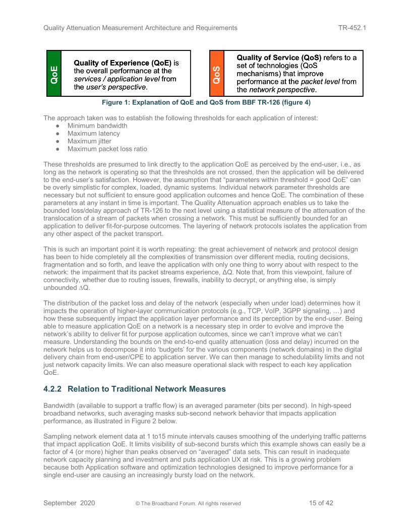
(Defines a standard set of Access Service Attributes that Service Providers useful to characterize the offered services. These may be used to determine the impact on customer experience.) TR-126 covered video, voice and web browsing/Internet access and it relates Quality of Experience (QoE) to Quality of Service (QoS) as shown in Figure 1 below.
Quality Attenuation Measurement Architecture and Requirements TR-452.1
September 2020 © The Broadband Forum. All rights reserved 15 of 42
Figure 1: Explanation of QoE and QoS from BBF TR-126 (figure 4)
The approach taken was to establish the following thresholds for each application of interest:
● Minimum bandwidth ● Maximum latency ● Maximum jitter ● Maximum packet loss ratio
These thresholds are presumed to link directly to the application QoE as perceived by the end-user, i.e., as long as the network is operating so that the thresholds are not crossed, then the application will be delivered to the end-user’s satisfaction. However, the assumption that “parameters within threshold = good QoE” can be overly simplistic for complex, loaded, dynamic systems. Individual network parameter thresholds are necessary but not sufficient to ensure good application outcomes and hence QoE. The combination of these parameters at any instant in time is important. The Quality Attenuation approach enables us to take the bounded loss/delay approach of TR-126 to the next level using a statistical measure of the attenuation of the translocation of a stream of packets when crossing a network. This must be sufficiently bounded for an application to deliver fit-for-purpose outcomes. The layering of network protocols isolates the application from any other aspect of the packet transport. This is such an important point it is worth repeating: the great achievement of network and protocol design has been to hide completely all the complexities of transmission over different media, routing decisions, fragmentation and so forth, and leave the application with only one thing to worry about with respect to the network: the impairment that its packet streams experience, ΔQ. Note that, from this viewpoint, failure of connectivity, whether due to routing issues, firewalls, inability to decrypt, or anything else, is simply unbounded ∆Q. The distribution of the packet loss and delay of the network (especially when under load) determines how it impacts the operation of higher-layer communication protocols (e.g., TCP, VoIP, 3GPP signaling, …) and how these subsequently impact the application layer performance and its perception by the end-user. Being able to measure application QoE on a network is a necessary step in order to evolve and improve the network’s ability to deliver fit for purpose application outcomes, since we can’t improve what we can’t measure. Understanding the bounds on the end-to-end quality attenuation (loss and delay) incurred on the network helps us to decompose it into ‘budgets’ for the various components (network domains) in the digital delivery chain from end-user/CPE to application server. We can then manage to schedulability limits and not just network capacity limits. We can also measure operational slack with respect to each key application QoE.
4.2.2 Relation to Traditional Network Measures
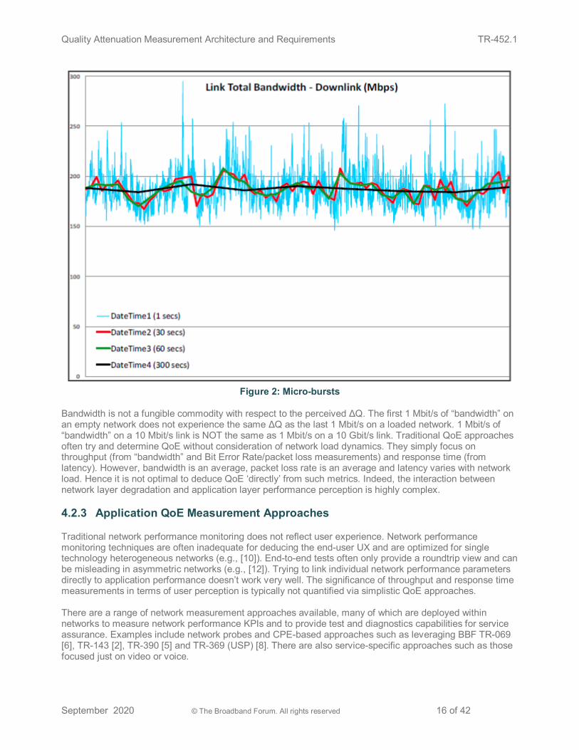
Bandwidth (available to support a traffic flow) is an averaged parameter (bits per second). In high-speed broadband networks, such averaging masks sub-second network behavior that impacts application performance, as illustrated in Figure 2 below. Sampling network element data at 1 to15 minute intervals causes smoothing of the underlying traffic patterns that impact application QoE. It limits visibility of sub-second bursts which this example shows can easily be a factor of 4 (or more) higher than peaks observed on “averaged” data sets. This can result in inadequate network capacity planning and investment and puts application UX at risk. This is a growing problem because both Application software and optimization technologies designed to improve performance for a single end-user are causing an increasingly bursty load on the network.
Quality Attenuation Measurement Architecture and Requirements TR-452.1
September 2020 © The Broadband Forum. All rights reserved 16 of 42
Figure 2: Micro-bursts
Bandwidth is not a fungible commodity with respect to the perceived ΔQ. The first 1 Mbit/s of “bandwidth” on an empty network does not experience the same ΔQ as the last 1 Mbit/s on a loaded network. 1 Mbit/s of “bandwidth” on a 10 Mbit/s link is NOT the same as 1 Mbit/s on a 10 Gbit/s link. Traditional QoE approaches often try and determine QoE without consideration of network load dynamics. They simply focus on throughput (from “bandwidth” and Bit Error Rate/packet loss measurements) and response time (from latency). However, bandwidth is an average, packet loss rate is an average and latency varies with network load. Hence it is not optimal to deduce QoE ‘directly’ from such metrics. Indeed, the interaction between network layer degradation and application layer performance perception is highly complex.
4.2.3 Application QoE Measurement Approaches
Traditional network performance monitoring does not reflect user experience. Network performance monitoring techniques are often inadequate for deducing the end-user UX and are optimized for single technology heterogeneous networks (e.g., [10]). End-to-end tests often only provide a roundtrip view and can be misleading in asymmetric networks (e.g., [12]). Trying to link individual network performance parameters directly to application performance doesn’t work very well. The significance of throughput and response time measurements in terms of user perception is typically not quantified via simplistic QoE approaches. There are a range of network measurement approaches available, many of which are deployed within networks to measure network performance KPIs and to provide test and diagnostics capabilities for service assurance. Examples include network probes and CPE-based approaches such as leveraging BBF TR-069 [6], TR-143 [2], TR-390 [5] and TR-369 (USP) [8]. There are also service-specific approaches such as those focused just on video or voice.
Quality Attenuation Measurement Architecture and Requirements TR-452.1
September 2020 © The Broadband Forum. All rights reserved 17 of 42
The techniques and vendor solutions cited above tend to be either network-centric or very application-specific. They are useful for network-level KPIs and assurance or for detailed service-specific performance diagnostics. However, they are sub-optimal for end-to-end QoE measurement. The paradox with network layer measurements is that often all network indicators are ‘green’, yet the delivered QoE is poor; or some network indicators are ‘red’, yet the delivered QoE is OK. This can be for a variety of reasons e.g., that the indicators are measuring parameters that are either not good proxies for QoE in their own right, or that the reporting is averaging data and hiding the events that impact QoE. It could also be that the measurement tool has a sampling rate that does not identify issues. Application Performance Management (APM) tools do exist but similarly do not provide a good proxy for the end-users’ experience, instead concentrating on system performance metrics. They often use a simple response time measurement of an application and provide no explanation of what network/IT infrastructure behavior or combination of system behaviors caused deterioration in performance or what impact that deterioration would have on end-users’ experience of the service. Also, they usually do not adequately isolate when network/IT infrastructure behavior caused deterioration as perceived by the user. The remedy for poor QoE is impossible to find if you don’t have the tools to identify and isolate the cause. Application layer QoE tools often see the effect but not the cause of problems and have little or no support for diagnosis. Hence, we need both application QoE tools and deep-dive network diagnostic tools to complement each other. It is easy to produce lots of data but much harder to extract actionable information.
4.2.4 Relating Network Quality to Application QoE
Our fundamental requirement is to be able to relate the packet-level quality attenuation (i.e., loss and delay) to the user experience ‘disappointment’ (e.g., failed calls, or slow web page load time). Once we understand that, we can go on to consider different control/data planes or flows within applications. This enables us to then answer questions such as:
● Which network slice should an application use? ● Do both data packets and control packets need to be given the same QoS treatment? ● Which clouds offer suitable performance for a particular application (private cloud, public cloud,
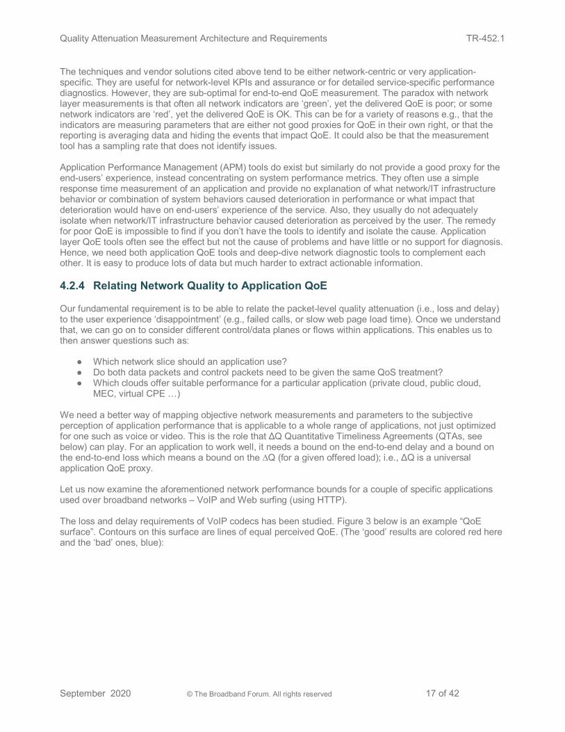
MEC, virtual CPE …) We need a better way of mapping objective network measurements and parameters to the subjective perception of application performance that is applicable to a whole range of applications, not just optimized for one such as voice or video. This is the role that ΔQ Quantitative Timeliness Agreements (QTAs, see below) can play. For an application to work well, it needs a bound on the end-to-end delay and a bound on the end-to-end loss which means a bound on the ∆Q (for a given offered load); i.e., ΔQ is a universal application QoE proxy. Let us now examine the aforementioned network performance bounds for a couple of specific applications used over broadband networks – VoIP and Web surfing (using HTTP). The loss and delay requirements of VoIP codecs has been studied. Figure 3 below is an example “QoE surface”. Contours on this surface are lines of equal perceived QoE. (The ‘good’ results are colored red here and the ‘bad’ ones, blue):
Quality Attenuation Measurement Architecture and Requirements TR-452.1
September 2020 © The Broadband Forum. All rights reserved 18 of 42
Figure 3: Example of a VoIP QoE Surface (from [16]) For VoIP a PESQ score of > 3.8 is considered ‘toll quality’. The network quality to application quality ‘surface’ is one approach to capture the relationship. Characterization permits the assessment of ‘trades’ that may need to be made during deployment. It also permits the assessment of risk(s) associated with inaccurately characterized quality requirements and how much variation can be tolerated. Note that there is an interesting interaction between how the codec works and its delay/loss sensitivity. Some “low bitrate” codecs can’t tolerate adverse network conditions. All codecs are NOT equal in this respect. This is just a means of illustrating the coupling between network performance and QoE for an important class of inelastic traffic flows. Note that, in this case, it is jitter (related to ∆Q|V) and loss rate that are the aspects of quality attenuation that most impact the UX. Now let us examine a QoE performance surface for a simple web surfing transaction (i.e., extracting information from a web site by an HTTP request).
Quality Attenuation Measurement Architecture and Requirements TR-452.1
September 2020 © The Broadband Forum. All rights reserved 19 of 42
Figure 4: HTTP Median Time to Complete
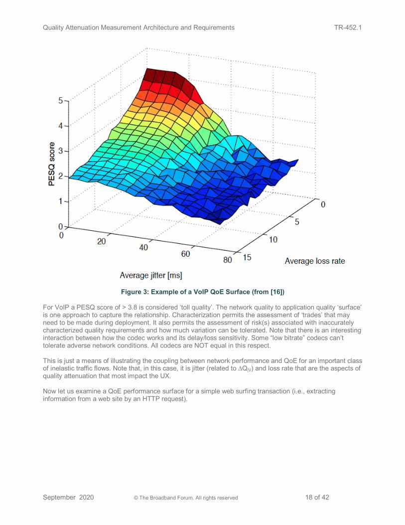
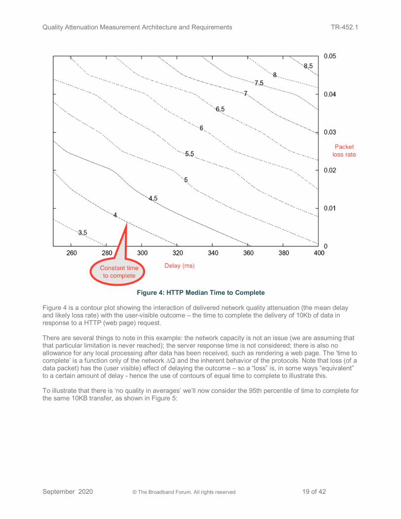
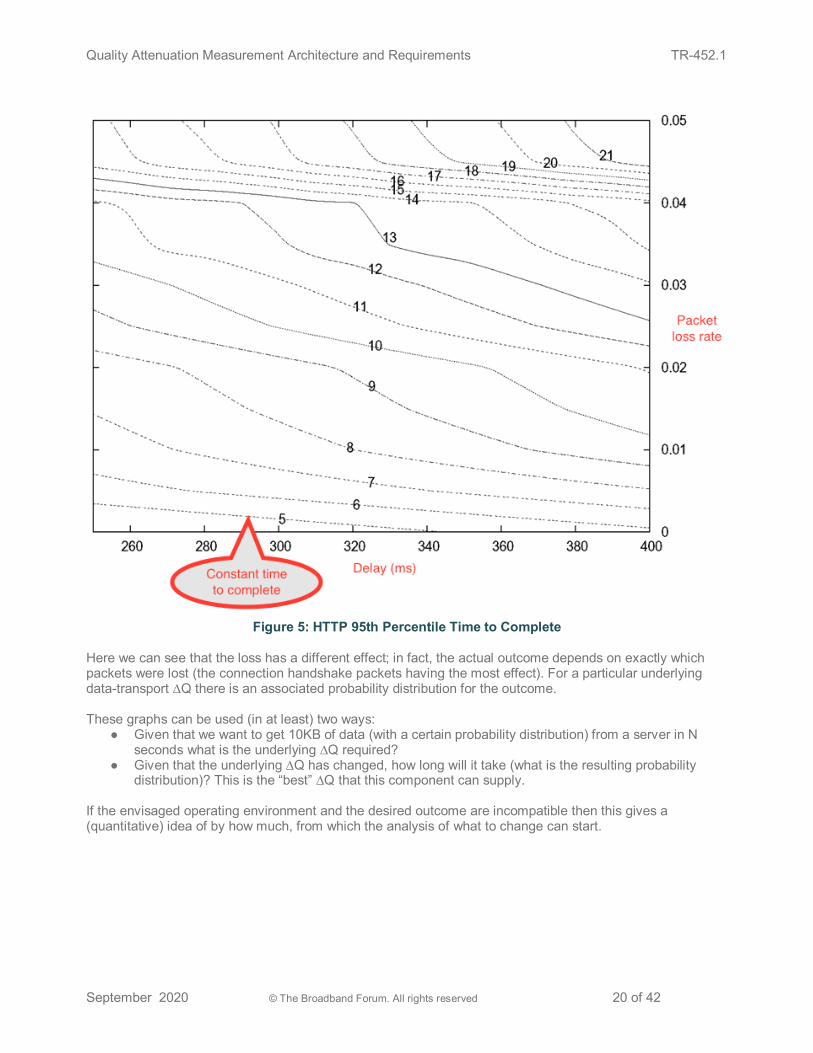
Figure 4 is a contour plot showing the interaction of delivered network quality attenuation (the mean delay and likely loss rate) with the user-visible outcome – the time to complete the delivery of 10Kb of data in response to a HTTP (web page) request. There are several things to note in this example: the network capacity is not an issue (we are assuming that that particular limitation is never reached); the server response time is not considered; there is also no allowance for any local processing after data has been received, such as rendering a web page. The ‘time to complete’ is a function only of the network ∆Q and the inherent behavior of the protocols. Note that loss (of a data packet) has the (user visible) effect of delaying the outcome – so a “loss” is, in some ways “equivalent” to a certain amount of delay - hence the use of contours of equal time to complete to illustrate this. To illustrate that there is ‘no quality in averages’ we’ll now consider the 95th percentile of time to complete for the same 10KB transfer, as shown in Figure 5:
Quality Attenuation Measurement Architecture and Requirements TR-452.1
September 2020 © The Broadband Forum. All rights reserved 20 of 42
Figure 5: HTTP 95th Percentile Time to Complete
Here we can see that the loss has a different effect; in fact, the actual outcome depends on exactly which packets were lost (the connection handshake packets having the most effect). For a particular underlying data-transport ∆Q there is an associated probability distribution for the outcome. These graphs can be used (in at least) two ways:
● Given that we want to get 10KB of data (with a certain probability distribution) from a server in N seconds what is the underlying ∆Q required?
● Given that the underlying ∆Q has changed, how long will it take (what is the resulting probability distribution)? This is the “best” ∆Q that this component can supply.
If the envisaged operating environment and the desired outcome are incompatible then this gives a (quantitative) idea of by how much, from which the analysis of what to change can start.
Quality Attenuation Measurement Architecture and Requirements TR-452.1
September 2020 © The Broadband Forum. All rights reserved 21 of 42
5 Measuring Network Quality Attenuation This section specifies quality attenuation in broadband packet networks and provides requirements to be able to measure it along a network path.
5.1 Outcomes and Observations We define an ‘outcome’ as something that can be observed to start at some point in time and may be observed to complete at some later time. This could be something long and complex, such as bidding to host the Olympic Games, and eventually holding the closing ceremony; note that in this case, if we lose the bid to hold the games, we will never hold the closing ceremony and so the outcome fails. In this document, we are concerned with much simpler outcomes such as translocating a packets-worth of information from one point to another; in this case the outcome starts when we begin sending the packet, and completes when the packet is fully received at its destination. If the packet is corrupted or dropped, this outcome fails. Note that the location where the outcome is observed to start may be different from that where it may be observed to complete, and so determining how long it takes to complete (and whether it does) is typically a distributed, or multi-point, measurement. An outcome may be parameterized in some way that influences how long it takes to complete. In the case of the Olympic Games, this could be whether we are considering the summer or winter games; in the case of a packet it would be the size of the packet. In the case of networks, as noted above, we are interested in the probability distribution of outcome duration/failure, for which we need sufficient measurements of individual outcomes to obtain a statistically valid estimate. Furthermore, achieving the overall outcome involves a number of packet-forwarding steps, each of which can be considered an outcome in its own right. Note that forwarding a packet (i.e., receiving and retransmitting it) involves four distinct timed events:
1. Packet starts being received; 2. Packet finishes being received; 3. Packet starts being transmitted; 4. Packet finishes being transmitted.
Typically, not all of this information may be available. However, if the bit-rate of an interface and the size of the packet is known, then the interval between the start and end of a packet reception/transmission on that interface can be deduced. Observing these events on distinct interfaces of a single network element enables the ∆Q through that element to be measured; more interesting, however, is to combine observations from different network elements to follow the transit of an individual packet along a network path, which can be extremely useful for localizing the source of undue quality attenuation.
Quality Attenuation Measurement Architecture and Requirements TR-452.1
September 2020 © The Broadband Forum. All rights reserved 22 of 42
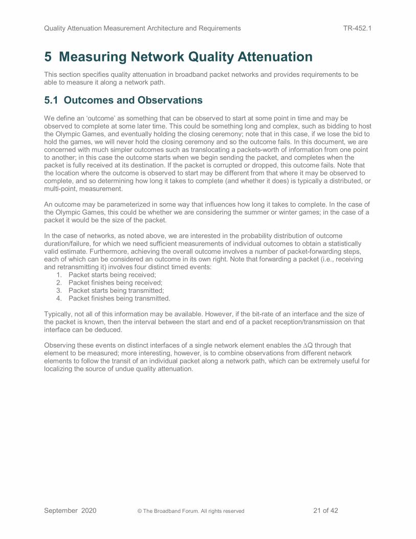
Figure 6: Multipoint observations
This leads to the situation illustrated in Figure 6, where sequences of observations are made at several points A, B, C,… This provides sufficient data to compute ∆QA→B, ∆QB→C, and ∆QA→C. Informative note: the compositionality of ∆Q, discussed in §7.2.1, guarantees that ∆QA→C = ∆QA→B ⊕ ∆QB→C. We call a point on the packet path at which observations can be made an Observation Point and abbreviate this to OP. Each OP may observe either packet receptions or packet transmissions. A network path involves at least two OPs. An element that forwards packets may implement an OP for receptions, transmissions or both. In the terminology of [4], an OP would be a function of a Measurement Agent. Since computing ∆Q involves comparing observations taken at different OPs, the observation information also needs to be translocated to a correlation and analysis function, which needs to able to match up observations of the same packet at different locations. This could be done at one or more points along the path or at an entirely different location. Observations can be translocated as a stream or in a batch. In the terminology of [4], this function is a Data Collector. Matching observations of the same packet within one or more streams of packets at different locations requires the observations reported from each location to include some characteristics that distinguish particular packets. Which characteristics are required will depend on the circumstances, and could be as simple as a sequence number. If more than one stream of packets is being observed, then information will also be required that distinguishes the streams, such as IP 5-tuple, DSCP marking etc. This leads to the following general requirements:
[R-1] An OP MUST be able to record the time at which events occur with a resolution of 10 microseconds or better. [R-2] An OP MUST be able to record the time between different events with a long-term accuracy of better than 100ppm. [R-3] For each observed packet received, an OP MUST be able to record AT LEAST THREE of the following:
a. the time at which a packet reception starts. b. the time at which a packet reception completes c. the bit-rate of the receiving interface. d. the size of a received packet.
[R-4] An OP MUST be able to record distinguishing characteristics of a received packet.
Quality Attenuation Measurement Architecture and Requirements TR-452.1
September 2020 © The Broadband Forum. All rights reserved 23 of 42
[R-5] For each observed packet transmitted, an OP MUST be able to record AT LEAST THREE of the following:
a. the time at which a packet transmission starts. b. the time at which a packet transmission completes c. the bit-rate of the transmitting interface. d. the size of a transmitted packet.
[R-6] An OP MUST be able to record distinguishing characteristics of a transmitted packet. [R-7] An OP MUST be able to report recorded observations (the information recorded according to requirements [R-3] to [R-6] to a correlation and analysis function.
In order to avoid an OP recording (and potentially reporting) spurious data it needs to be appropriately controlled:
[R-8] The OP MUST be able to be enabled and disabled (e.g., for CPE, using TR-069 or USP). [R-9] The OP SHOULD be configurable with a maximum number of observations to record. [R-10] The OP SHOULD be configurable with a maximum time over which to record observations. [R-11] The maximum number and maximum time SHOULD be resettable. [R-12] The protocol used to control the OP MUST use authentication.
Note that the optionality of [R-9], [R-10] and [R-11] is intended to support low-complexity implementations, on the basis that [R-7] provides a mitigation of any issues that might arise from not providing this functionality.
5.1.1 Data collection and correlation
It is not necessary for the purposes of analyzing the test data to record the entire packet. The essential information for determining ∆Q is:
• The identifier of the measurement stream to which the packet belongs • The size of both:
o The information whose timing is being observed, and o The overhead involved in transporting this
• Sufficient packet contents to uniquely identify the packet within the measurement stream, such as: o A test packet sequence number (which can be short) o A hash of the packet contents (avoiding any parts that may be changed in transit such as
TTL) • The local time at which the packet was observed.
5.2 Calculating ΔQ from Observations Turning sets of observations provided by OPs into reliable measures of ∆Q involves several steps:
• Correlating observation times of the same packet at different OPs o This includes inferring loss
• Correcting for systematic clock differences between different OPs (e.g., clock offset) • Extracting components of ∆Q
Note that these steps may be performed iteratively, for example the decomposition of ∆Q can be used for clock offset correction when the measurement path includes a round-trip.
5.2.1 Decomposing ∆Q
In essence, the ΔQ approach represents data transport quality as a set of distributions of delay with associated probabilities of loss. These can conveniently be broken into three “components”:
Quality Attenuation Measurement Architecture and Requirements TR-452.1
September 2020 © The Broadband Forum. All rights reserved 24 of 42
• ΔQ|G This is the distribution of inherent delay and probability of loss introduced by the path itself, which includes the time taken for signals to traverse it. It can be thought as the minimum time taken for a hypothetical zero-length packet to travel the path. In many cases this is effectively constant for relatively long periods of time, in which case it can be represented by a single delay value. For typical broadband networks, a convenient unit is ms. If characteristics of the path result in a baseline loss rate that is independent of packet size, this is included here.
• ΔQ|S This distribution is that part of ΔQ that is a function of packet size and incorporates things like serialization and de-serialization time. ΔQ|S is a function from packet size to delay, which is usually monotonic and in many cases is broadly linear, in which case we can represent it by a simple slope parameter, with the dimensions of time/length. For current network interface speeds, a convenient unit is µs/byte. If characteristics of the path result in a baseline loss rate that depends on packet size, for example due to a constant probability of corruption of each byte, this is included here.
• ΔQ|V This is the distribution of delay and loss introduced by the fact that the network is non-idle, therefore it is affected by any other packets on the system, including those generated by the same application and user. This is modelled as a random variable, whose distribution may vary by time of day etc.. This can typically not be reduced to a single number, although moments of the distribution can be useful. The zeroth moment is the total probability, whose difference from one represents loss; the first moment is the mean variable delay, measured in s; the second central moment is the variance, whose square root is the standard deviation, also measured in s. Loss that results from competition for shared finite resources such as interface packet buffering is included here.
The ΔQA→B of the path (A,B) is characterized by the [G, S, V] tuple. Note that obtaining reliable estimates of G and S requires a sufficient spread of packet sizes, which leads to the following requirements on the packets being observed (whether these are normal data packets, injected test packets, or a mixture):
[R-13] The stream of packets being observed at OPs along a path MUST have a spread of sizes. [R-14] The ratio between the smallest and largest packets in the stream MUST be at least 10. [R-15] The number of different sizes in the packet stream MUST be at least 5. [R-16] The number of packets in the stream with each size MUST be approximately equal.
Raw ΔQ measurements produce a scatter plot of points characterized by [size, delay] tuples. Plotting measured packet delay versus measurement time instance reveals little structure. However, plotting measured packet delay versus packet size shows that for the same packet size, there is variability in the delay which is a function of instantaneous load on the various network elements. With a sufficient number of measurements, the minimum delay for each packet size in the scatter plot is attained when the variable delay due to contention is close to zero (i.e., V ~ 0). An example is shown in Figure 7 below:

Quality Attenuation Measurement Architecture and Requirements TR-452.1
September 2020 © The Broadband Forum. All rights reserved 25 of 42
Figure 7: Packet delay measurement versus packet size (for an Ethernet switch) The basic processing steps for the calculation of ΔQ components from a set of measurements can be summarized as follows:
1. Arrange the population of measurement results by packet size to obtain an array of: {pktID, pktsize, ΔQ(pktsize)}
2. Construct the measurement sample population: {pktID, pktsize, min ΔQ(pktsize)}
3. Use linear regression to fit a line through this population Undertake the above processing steps separately for each pair of OPs and directions. This approach relies on two assumptions:
1. Larger packets take at least as long to transmit on average as smaller ones (i.e., ∆Q|S is a monotonic increasing function of packet size);
2. At least some of the sample packets of any given size (bucket) experience negligible delay from contention for resources (i.e., the minimum of the set of samples from ∆Q|V tends to zero as the sample size increases).
Note that, in order to meet assumption (2) above, it may be advantageous to group packet sizes into buckets of similar sizes to increase the sample size in each bucket. On these assumptions, the statistical model for the data points representing the minimum delay value for each packet size can be approximated by a linear model, i.e., a straight line.
Delay Min (size) = m x size + G Where G is the delay introduced by the network on a hypothetical zero length packet (no serialization delays etc.); i.e., it is the intercept on the y-axis of the regression line through the set of minimum delays per packet size.
Quality Attenuation Measurement Architecture and Requirements TR-452.1
September 2020 © The Broadband Forum. All rights reserved 26 of 42
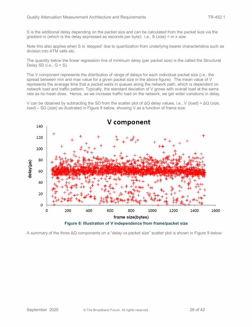
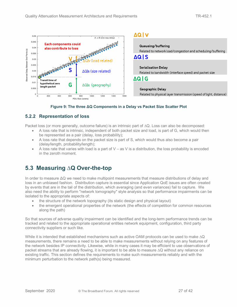
S is the additional delay depending on the packet size and can be calculated from the packet size via the gradient m (which is the delay expressed as seconds per byte); i.e., S (size) = m x size. Note this also applies when S is ‘stepped’ due to quantization from underlying bearer characteristics such as division into ATM cells etc. The quantity below the linear regression line of minimum delay (per packet size) is the called the Structural Delay SD (i.e., G + S). The V component represents the distribution of range of delays for each individual packet size (i.e., the spread between min and max value for a given packet size in the above figure). The mean value of V represents the average time that a packet waits in queues along the network path, which is dependent on network load and traffic pattern. Typically, the standard deviation of V grows with overall load at the same rate as its mean does. Hence, as we increase traffic load on the network, we get wider variations in delay. V can be obtained by subtracting the SD from the scatter plot of ΔQ delay values, i.e., V (load) = ΔQ (size, load) – SD (size) as illustrated in Figure 8 below, showing V as a function of frame size:
Figure 8: Illustration of V independence from frame/packet size
A summary of the three ΔQ components on a “delay vs packet size” scatter plot is shown in Figure 9 below:
Quality Attenuation Measurement Architecture and Requirements TR-452.1
September 2020 © The Broadband Forum. All rights reserved 27 of 42
Figure 9: The three ΔQ Components in a Delay vs Packet Size Scatter Plot
5.2.2 Representation of loss
Packet loss (or more generally, outcome failure) is an intrinsic part of ∆Q. Loss can also be decomposed: • A loss rate that is intrinsic, independent of both packet size and load, is part of G, which would then
be represented as a pair (delay, loss probability); • A loss rate that depends on the packet size is part of S, which would thus also become a pair
(delay/length, probability/length); • A loss rate that varies with load is a part of V – as V is a distribution, the loss probability is encoded
in the zeroth moment.
5.3 Measuring ∆Q Over-the-top In order to measure ΔQ we need to make multipoint measurements that measure distributions of delay and loss in an unbiased fashion. Distribution capture is essential since Application QoE issues are often created by events that are in the tail of the distribution, which averaging (and even variances) fail to capture. We also need the ability to perform "network tomography" style analysis so that performance impairments can be isolated to the appropriate aspects of:
• the structure of the network topography (its static design and physical layout) • the emergent operational properties of the network (the effects of competition for common resources
along the path) So that sources of adverse quality impairment can be identified and the long-term performance trends can be tracked and related to the appropriate operational entities network equipment, configuration, third party connectivity suppliers or such like. While it is intended that established mechanisms such as active OAM protocols can be used to make ∆Q measurements, there remains a need to be able to make measurements without relying on any features of the network besides IP connectivity. Likewise, while in many cases it may be efficient to use observations of packet streams that are already flowing, it is important to be able to measure ∆Q without any reliance on existing traffic. This section defines the requirements to make such measurements reliably and with the minimum perturbation to the network path(s) being measured.
Quality Attenuation Measurement Architecture and Requirements TR-452.1
September 2020 © The Broadband Forum. All rights reserved 28 of 42
5.3.1 Packet Generation
If we are unable to measure ∆Q by relying on existing traffic we must inject a stream of test packets. This requires a Packet Generator function (abbreviated PG). In the terminology of [4], this function would be performed by a Measurement Agent.
[R-17] The PG MUST be able to generate IP packets that will be routed along the path of interest. [R-18] The PG MUST generate IP packets of at least 5 different sizes. [R-19] The ratio between the smallest and largest packets generated by the PG MUST be at least 10. [R-20] The PG SHOULD be able to select the size of each packet pseudo-randomly. [R-21] The PG SHOULD be able to adjust the interval between generated packets so that the average bit-rate is constant. [R-22] The PG MUST be able to reproduce the sequence of packet sizes and inter-packet gaps (so that reproducible loads can be applied for fault isolation and regression testing).
It is essential that the PG can be controlled. In the terminology of [4], this would be performed by a Measurement Controller. The following requirements are designed to limit opportunities for excessive resource consumption, whether due to misconfiguration or malicious action.
[R-23] The PG MUST be able to be started and stopped (e.g., using TR-069 or USP). [R-24] The PG MUST be configurable with a maximum average data rate. [R-25] The PG MUST be configurable with a maximum packet rate. [R-26] The PG MUST be configurable with a maximum time over which to send packets. [R-27] The control interface of the PG SHOULD be suitably authenticated.
5.3.2 Packet Reflection
It is advantageous to create a round-trip path so that the ∆Q of both outward and return paths (including their loss rates) can be measured at the same time. This can be achieved by adding a Packet Reflector function (abbreviated PR) that receives the packets sent by the PG and returns them to the originating point (by appropriate transposition of addressing information). In the terminology of [4], this would be performed by a Measurement Agent. In principle, it could be performed by a Measurement Peer, but this would violate [R-30] below.
[R-28] The PR MUST be able to return IP packets to the PG along the path of interest. [R-29] The PR MUST NOT alter the size of the packet when returning it to the PG.
It is essential that the PR can be controlled. The following requirements are designed to limit opportunities for excessive resource consumption, whether due to misconfiguration or malicious action.
[R-30] The PR MUST be able to be started and stopped (e.g., using TR-069 or USP). [R-31] The PR SHOULD be configurable with a maximum average data rate. [R-32] The PR SHOULD be configurable with a maximum packet rate. [R-33] The PR SHOULD be configurable with a maximum time over which to reflect packets. [R-34] The control interface of the PR SHOULD be suitably authenticated.
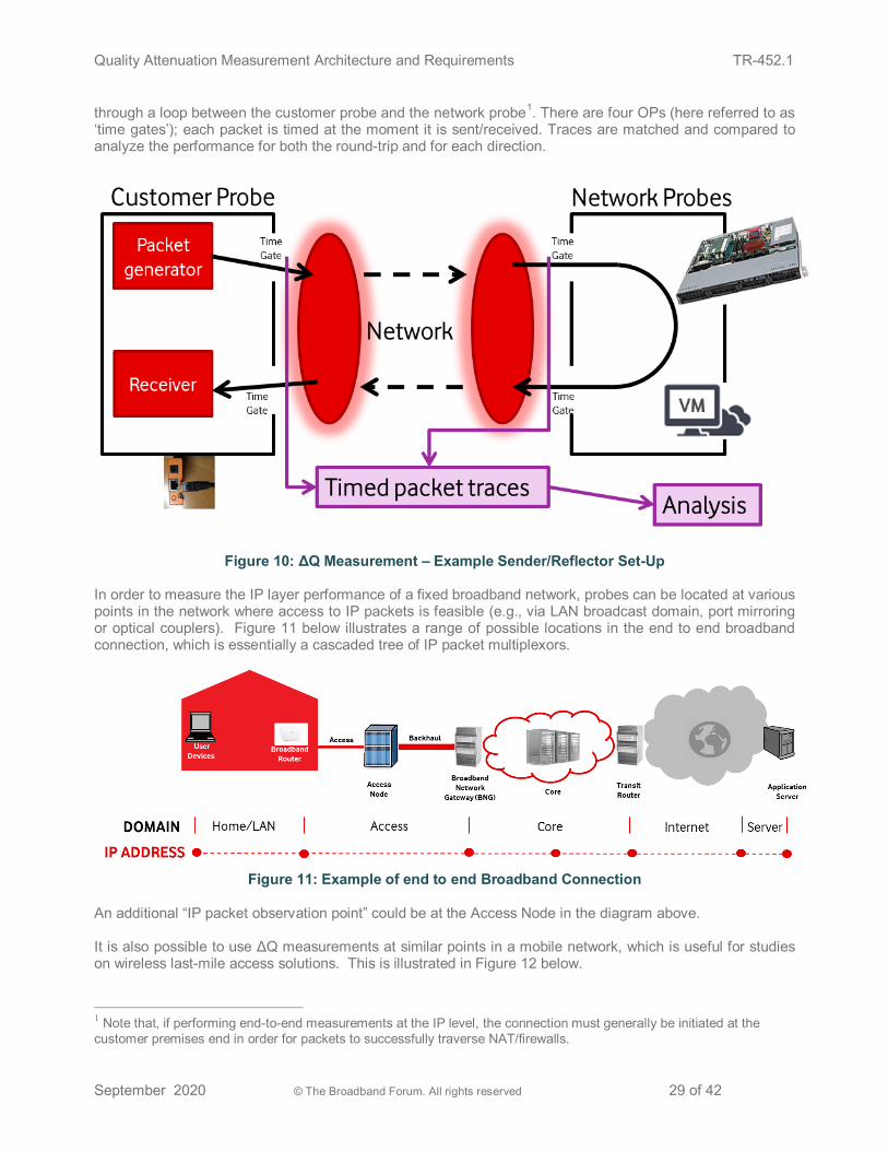
Reflected packets are received and discarded by a receiver co-located with the PG. Figure 10 below illustrates a basic ΔQ measurement configuration for broadband networks comprising a packet generator, packet reflector and packet receiver. The functions of generating/reflecting packets and performing observations are combined in specific network elements called ‘probes’. Each packet is sent
Quality Attenuation Measurement Architecture and Requirements TR-452.1
September 2020 © The Broadband Forum. All rights reserved 29 of 42
through a loop between the customer probe and the network probe1. There are four OPs (here referred to as ‘time gates’); each packet is timed at the moment it is sent/received. Traces are matched and compared to analyze the performance for both the round-trip and for each direction.
Figure 10: ΔQ Measurement – Example Sender/Reflector Set-Up In order to measure the IP layer performance of a fixed broadband network, probes can be located at various points in the network where access to IP packets is feasible (e.g., via LAN broadcast domain, port mirroring or optical couplers). Figure 11 below illustrates a range of possible locations in the end to end broadband connection, which is essentially a cascaded tree of IP packet multiplexors.
Figure 11: Example of end to end Broadband Connection
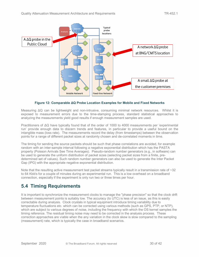
An additional “IP packet observation point” could be at the Access Node in the diagram above. It is also possible to use ΔQ measurements at similar points in a mobile network, which is useful for studies on wireless last-mile access solutions. This is illustrated in Figure 12 below.
1 Note that, if performing end-to-end measurements at the IP level, the connection must generally be initiated at the customer premises end in order for packets to successfully traverse NAT/firewalls.
Quality Attenuation Measurement Architecture and Requirements TR-452.1
September 2020 © The Broadband Forum. All rights reserved 30 of 42
Figure 12: Comparable ΔQ Probe Location Examples for Mobile and Fixed Networks Measuring ΔQ can be lightweight and non-intrusive, consuming minimal network resources. Whilst it is exposed to measurement errors due to the time-stamping process, standard statistical approaches to analyzing the measurements yield good results if enough measurement samples are used. Practitioners of ΔQ have typically found that of the order of 1000 to 4000 measurements per ‘experimental run’ provide enough data to discern trends and features, in particular to provide a useful bound on the intangible mass (loss rate). The measurements record the delay (from timestamps) between the observation points for a range of different packet sizes at randomly chosen and de-correlated moments in time. The timing for sending the source packets should be such that phase correlations are avoided, for example random with an inter-sample interval following a negative exponential distribution which has the PASTA property (Poisson Arrivals See Time Averages). Pseudo-random number generators (e.g., in software) can be used to generate the uniform distribution of packet sizes (selecting packet sizes from a finite, pre-determined set of values). Such random number generators can also be used to generate the Inter Packet Gap (IPG) with the appropriate negative exponential distribution. Note that the resulting active measurement test packet streams typically result in a transmission rate of ~32 to 64 Kbit/s for a couple of minutes during an experimental run. This is a low overhead on a broadband connection, especially if the experiment is only run two or three times per hour.
5.4 Timing Requirements It is important to synchronize the measurement clocks to manage the "phase precision" so that the clock drift between measurement points is suitably low. The accuracy (to UTC) is less of an issue, as this is easily correctable during analysis. Clock crystals in typical equipment introduce timing variability due to temperature fluctuations etc. which can be corrected using various methods (such as GPS, PTP, or NTP), which are subject to various degrees of noise, including the frequency with which the OS kernel samples the timing reference. The residual timing noise may need to be corrected in the analysis process. These correction approaches are viable when the any variation in the clock skew is slow compared to the sampling (measurement) rate, which is typically the case in broadband scenarios.
Quality Attenuation Measurement Architecture and Requirements TR-452.1
September 2020 © The Broadband Forum. All rights reserved 31 of 42
The need for such “clock mismatch compensation” techniques depends on the measurement objective and its associated precision requirements. So, for example, if seeking to assess the transit latency performance of a switch or router in isolation (or to compare different software versions), a service provider may seek to measure its G (µs) and S (ns/byte) capability. Exploiting the statistical properties of ∆Q avoids the need for measurement instrumentation accuracies at the ns level (as opposed to µs level). Note that clock drift is not an issue when all measurements are referred to the same clock (e.g., in a lab). If seeking to compare the performance of QoS mechanisms, the requisite instrumentation granularity should also be considered. It should be noted that a naive insistence upon accurate timing would limit the applicability of the Quality Attenuation approach, and hence appropriate precision analysis is important. The analysis approach outlined here avoids the need for all the measurement points have to be in the same clock domain, so the ΔQ measurement system can work across management domain boundaries (e.g., between different network providers in an end-to-end connection, which is where the clock domain boundaries tend to lie). The analysis process can identify and resolve this issue of accuracy, precision and drift, so as to enable the use of disjoint clock domains. If the clock drift is too high, results can be rejected as errored. Uncorrected clock drift shows up as a drift in ∆Q|G, but suitable choice of observation points can cancel this out. The analysis system can exploit the invariant (operational assumption) that, between two points the sum of the ∆Q|G in each direction should be stationary (which it is irrespective of clock drift). After completing a ΔQ experiment, the resulting identifiable (e.g., via unique experiment identifier) packet timestamps from all measurement nodes can be recorded in a back-end database.
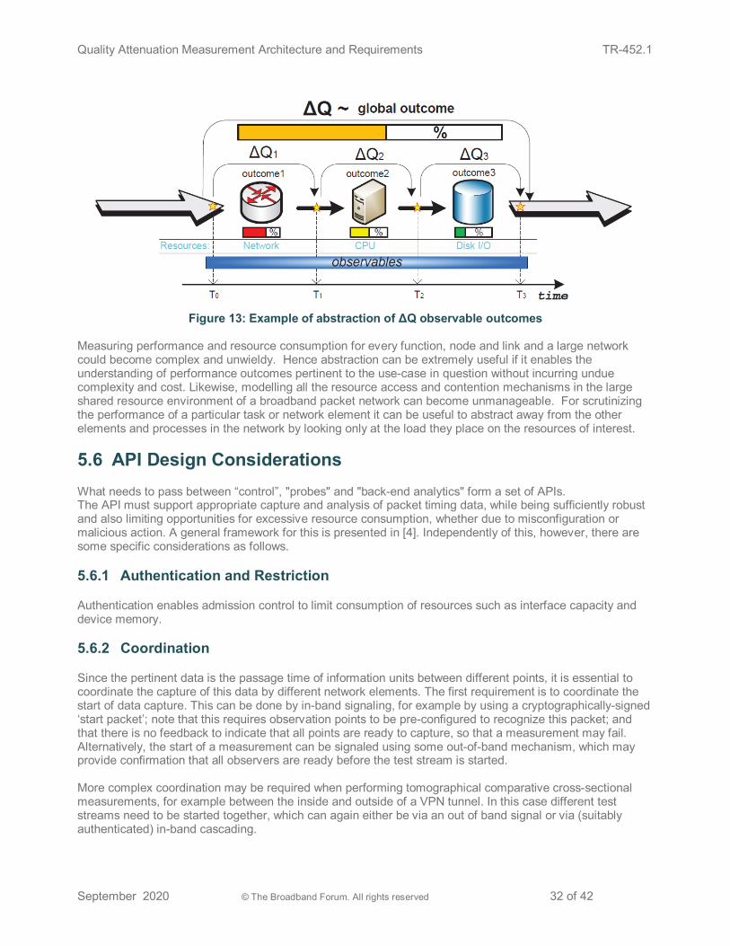
5.5 Abstraction and Choice of Measurement Locations The measurement of ΔQ enables us to reason about the performance characteristics of a network in a way that abstracts us away from the implementation details of the network. This abstraction can be at various levels depending on our chosen granularity for the observation (measurement) points. It can for example be applied to international, national, local or home networks. It can also be applied to individual network links and elements, such as switches and routers. The G and S components could be used to compare the performance of various equipment types, vendor implementations or physical versus virtualized implementations. The V component can provide useful information to understand traffic pattern properties. An example of abstracting ΔQ to a higher level is illustrated in Figure 13 below. Here, a system such as a network node involves use of network, processing and storage resources. This could be typical of a virtualized network node implemented on generic computer hardware. It has three main tasks: Receive some data from the network, perform some compute processing on that data and then store the outcome. We can measure ΔQ outcomes for each of these constituent tasks or we can choose to abstract the ΔQ to a single global outcome treating the three resource domains in the network element as a single aggregate resource. Note that, because ∆Q is conserved, if the aggregate ∆Q is within some designated limit, then all the ∆Qs for the constituent tasks must also be suitably bounded.
Quality Attenuation Measurement Architecture and Requirements TR-452.1
September 2020 © The Broadband Forum. All rights reserved 32 of 42
Figure 13: Example of abstraction of ΔQ observable outcomes
Measuring performance and resource consumption for every function, node and link and a large network could become complex and unwieldy. Hence abstraction can be extremely useful if it enables the understanding of performance outcomes pertinent to the use-case in question without incurring undue complexity and cost. Likewise, modelling all the resource access and contention mechanisms in the large shared resource environment of a broadband packet network can become unmanageable. For scrutinizing the performance of a particular task or network element it can be useful to abstract away from the other elements and processes in the network by looking only at the load they place on the resources of interest.
5.6 API Design Considerations What needs to pass between “control”, "probes" and "back-end analytics" form a set of APIs. The API must support appropriate capture and analysis of packet timing data, while being sufficiently robust and also limiting opportunities for excessive resource consumption, whether due to misconfiguration or malicious action. A general framework for this is presented in [4]. Independently of this, however, there are some specific considerations as follows.
5.6.1 Authentication and Restriction
Authentication enables admission control to limit consumption of resources such as interface capacity and device memory.
5.6.2 Coordination
Since the pertinent data is the passage time of information units between different points, it is essential to coordinate the capture of this data by different network elements. The first requirement is to coordinate the start of data capture. This can be done by in-band signaling, for example by using a cryptographically-signed ‘start packet’; note that this requires observation points to be pre-configured to recognize this packet; and that there is no feedback to indicate that all points are ready to capture, so that a measurement may fail. Alternatively, the start of a measurement can be signaled using some out-of-band mechanism, which may provide confirmation that all observers are ready before the test stream is started. More complex coordination may be required when performing tomographical comparative cross-sectional measurements, for example between the inside and outside of a VPN tunnel. In this case different test streams need to be started together, which can again either be via an out of band signal or via (suitably authenticated) in-band cascading.
Quality Attenuation Measurement Architecture and Requirements TR-452.1
September 2020 © The Broadband Forum. All rights reserved 33 of 42
Since it may be the case that more than one measurement stream is being observed by a given network element, it is important that each stream has an associated unique identifier, which should be set up as part of the observation start coordination. Note that it is not desirable for such an identifier to be present in every packet of the measurement stream, since this increases the minimum size of the measurement packets; rather different measurement streams should be distinguished by aspects of the packet headers. Note that encapsulation/decapsulation along a path may change the offset at which the relevant information is found, which needs to be configured before the measurement starts.
Quality Attenuation Measurement Architecture and Requirements TR-452.1
September 2020 © The Broadband Forum. All rights reserved 34 of 42
6 Use Cases
6.1 Network Health Check ΔQ probes could be distributed at strategic locations around a network such as key regional aggregation nodes/PoPs, transit/peering points and 3rd-party interconnects. They could also be deployed on a few access connections in each regional aggregation area (e.g., spread across different access technologies / platforms) to act as “sensors”. This “sub-sampling” of every network node and link can give an indication of the overall health of the network and potentially an early warning system for potential performance degradation (ideally before it becomes customer affecting), be that due to congestion, failure or a breach of the network’s “Predictable Region of Operation” (PRO). Examples of the sort of performance insight questions that could be answered by this approach include:
• Is the architecture appropriate? • Are the network assets being fully used? • Are there loading issues? • Are the configurations consistent with performance goals? • Is the capacity planning process effective?
o Does it meet the requirements of the services and applications? o If not, what are the impairments? o Where are they occurring?
• What new services could be supported? o What would be the impact on existing services if they were rolled out?
In addition, a network audit using Quality Attenuation measurements could also be used to answer questions related to capacity and schedulability such as:
● What are the structural contributions to QoE impairment? ● Where is capacity being used to cover up scheduling issues? ● How efficiently are ephemeral resources being allocated?
○ Voice transport ○ Signaling/control ○ Data transport
Such insights can help a network operator to more effectively sweat their network assets before spending more capex, or to improve QoE without incurring unnecessary expense.
6.2 Root Cause Analysis (RCA) Tool for Networks Operations Teams
Network Operations Centers (NOCs) have a variety of existing tools to provide visibility of the network and to assure its performance. The use of Quality Attenuation via ΔQ measurements could potentially compliment these to give greater insight into issues that some other tools find hard to spot (especially those that just average ‘performance’ via 15-minute counters). For example, misconfigured schedulers can be an extremely elusive problem to diagnose. The ΔQ measurement process itself (a statistical one) is applicable in an operational network environment using lightweight processes that consume negligible resources. Indeed, some measurement capabilities could be created “on demand” e.g., instantiating a virtual probe to provide ΔQ measurements from a virtual CPE device on the customer premises, then relinquishing the resources (memory and CPU) once the measurement results have been captured.
Quality Attenuation Measurement Architecture and Requirements TR-452.1
September 2020 © The Broadband Forum. All rights reserved 35 of 42
Examples of observable phenomenon via Quality Attenuation measurements include:
● Unexpected re-routing ● Inappropriate load balancing ● Packet fragmentation ● DSL Dynamic Line Management (DLM) & Seamless Rate Adaptation (SRA) profile changes ● CPE processor maxed out and impact of Wi-Fi scanning “distracting” from packet processing ● Misconfigured schedulers (queue saturation & bufferbloat etc.) ● QoS benefits/differentiation under congestion ● Maxed out transmission links ● Technology and architecture upgrades ● 3G to 4G bearer change on FMS
ΔQ measurement capabilities could be integrated with the NOC’s network and system monitoring tools and with expert systems (increasingly using AI and machine learning) for fault analysis by analyzing the key ΔQ components and capturing their moving time series trend. This would allow a proactive detection of application degradation as opposed to many current tools which offer averaged values with a lag of several minutes. A certain increase in the instantaneous delay or delay variation is a sign that traffic is suffering increased queueing and alarms or actions could be triggered.
6.3 Network Technology Performance Characterization Not all bandwidth delivers the same ΔQ. For example:
• 50 Mbit/s on VDSL is NOT the same as 50 Mbit/s on GPON • 50 Mbit/s on a 100 Mbit/s Ethernet port is NOT the same as 50 Mbit/s on a 10 Gbit/s port • 1/10th of 100Mbit/s is NOT the same as 10 Mbit/s • 50 Mbit/s on an empty network is NOT the same as 50 Mbit/s on a loaded network
Network performance is about more than just having ‘enough bandwidth’. Different broadband access technologies have very different physical layer characteristics. Some, like Passive Optical Networks (PON) and Cable modems provide access to a common physical media which is shared among multiple customers. Others have more point-to-point centric connectivity. Some physical bearers like metallic twisted pairs and (to a lesser extent) coaxial cable can suffer from external noise ingress such as radio frequency interference or impulse noise. Consequently, the modem “bit-pumps” operate in different ways for different technologies in order to deal with such bearer-specific issues. Examples include the specifics of error correction coding, interleaving and physical layer retransmission. This impacts the nature of physical layer bit errors (e.g., single, bursty, clustered etc.) which in turn impacts how such events manifest themselves at the IP packet layer (in terms of packet loss pattern, delay/jitter). Some broadband access connectivity approaches such as Hybrid Access (fixed-mobile bonding) can have quite complex performance characteristics due to the fixed and mobile links having very different latency and consistency characteristics. The “policy management” of such systems can dictate when the mobile link is enabled and what traffic or application types should flow over it (as opposed to staying on the fixed link). The policy also impacts the hysteresis of the system (when the mobile “booster” link is turned-off). Quality Attenuation measurements can be used to characterize the performance of such complex systems and to identify risks (hazards) in their operation, some of which may be mitigated by subsequent adjustment to the dynamics of the policy management operation. In summary, Quality Attenuation measurements can be used to characterize the performance of different technologies (even if they nominally deliver the same bandwidth) which helps an operator to understand how they may impact the delivery of customer applications and services.
Quality Attenuation Measurement Architecture and Requirements TR-452.1
September 2020 © The Broadband Forum. All rights reserved 36 of 42
6.4 Input to Network Architecture Design/Analysis Quality Attenuation performance analysis can be used for measurement in live networks, measurement in the lab but also in mathematical models. The latter can be used to reason about the performance implications of different network architectures and design approaches before the network is built and can help to give answers before costly trials are deployed. In turn, lab and field measurements can be used to inform the models to refine them and to undertake “what if” scenario analysis. For example, a network model informed by ΔQ measurements is able to provide a predictive capability in case different operating conditions are experienced, e.g., to evaluate the impact of increased network traffic loading and to quantify the consequent increased delays in the network. Hence this can provide a useful capability for network architects and designers. The architecting and design (including dimensioning) of networks often relies on average values like bandwidth. However, the required loss and delay performance metrics (which are instantaneous characteristics previously difficult to predict at design stage) do have an impact on the scalability of the network and also on its behavior close to saturation. For network architects, Quality Attenuation can provide an end-to-end network performance description, using its piecewise convolution properties for the performance contribution of the various links and nodes (network devices) that the network is comprised of. It can also provide a measure of the delay caused by queueing. Using this information in a comparison with theoretical traffic queueing models can enable the performance to be inferred for different traffic loads and traffic arrival patterns. Some examples of the sort of architecture and design decisions that could be informed by Quality Attenuation modelling and measurements include:
● Performance implications of locating a Virtual Network Function (VNF) at different nodes within the network or Internet. For example, on virtual CPE versus the network edge (as per MEC) versus a centralized private cloud (network operator’s data canter) versus a public cloud
● As above but for a content cache or CDN node ● Performance of different network slices, e.g., “standard” versus Ultra-Low Latency (ULL) ● The ability to compare the relative performance of different network equipment implementation
approaches. For example, comparing an ASIC-based element (such as physical BNG data plane) versus a commodity hardware-based data plane used by a vBNG VNF.
6.5 Equipment Selection Quality Attenuation measurements can be used to establish the relative performance characteristics of different models of network equipment which can then be used for comparison purposes. For example, a lab set up with a simple network can be used to measure the ΔQ when the network is operating with different types (models/vendors) of equipment that relay the IP packets (switch, router, Access Node, BNG etc.). The ΔQ components are derived from a number of measurement samples using a linear statistical dependency of the delay on the packet size as described in the Appendix §7. From this, the Structural Delay components of the performance attenuation introduced by the network device (known as G and S) can be calculated. The Structural Delay of the network device encompasses its immutable properties, e.g., access to the medium, serialization/deserialization delays and switching speed. This approach can therefore be used to establish which equipment meets requirements or is “best” (in the sense of introducing lowest latency due to packet processing). Service providers could use this as part of their RFQ process to select equipment or establish its compliance against requirements. The network device under test is simply treated as a black box that will delay IP packets. A differential paths approach can be used whereby we identify pairs of measurement points, i.e., network interfaces which communicate between them on path segments sharing the network devices. By measuring G and S for these paths we are able to extract the Structural Delay property for the “network device difference” (from §5.7.1.2 of reference [17]).
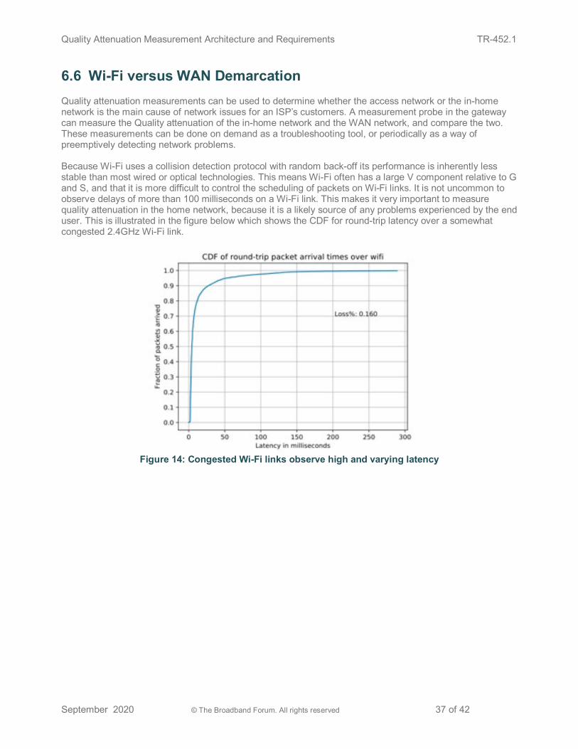
Quality Attenuation Measurement Architecture and Requirements TR-452.1
September 2020 © The Broadband Forum. All rights reserved 37 of 42
6.6 Wi-Fi versus WAN Demarcation Quality attenuation measurements can be used to determine whether the access network or the in-home network is the main cause of network issues for an ISP’s customers. A measurement probe in the gateway can measure the Quality attenuation of the in-home network and the WAN network, and compare the two. These measurements can be done on demand as a troubleshooting tool, or periodically as a way of preemptively detecting network problems. Because Wi-Fi uses a collision detection protocol with random back-off its performance is inherently less stable than most wired or optical technologies. This means Wi-Fi often has a large V component relative to G and S, and that it is more difficult to control the scheduling of packets on Wi-Fi links. It is not uncommon to observe delays of more than 100 milliseconds on a Wi-Fi link. This makes it very important to measure quality attenuation in the home network, because it is a likely source of any problems experienced by the end user. This is illustrated in the figure below which shows the CDF for round-trip latency over a somewhat congested 2.4GHz Wi-Fi link.
Figure 14: Congested Wi-Fi links observe high and varying latency
Quality Attenuation Measurement Architecture and Requirements TR-452.1
September 2020 © The Broadband Forum. All rights reserved 38 of 42
7 Appendix: Theoretical Background
7.1 Computation, Communication and ICT Fifty years ago, as data communications was emerging, the boundary between ‘communication’ and ‘computation’ was relatively clear. Communication took place over circuits constructed on a mainly analogue basis, with the analogue/digital conversion occurring at the network edges. For example, in Time-Division Multiplexing (TDM) the digital component is primarily shift buffers and framing. Computation occurred in a limited number of very specialized locations, containing mainframes (or, later, minicomputers). Even though those computers consisted of many components that exchanged data (processors, memory, disk drives), these exchanges were not in the same conceptual category as communications. The dominant mode of use was that the edges transferred data (punch card or line-printer images, characters to/from terminals) via communication links to the central location. The computation was centralized; the edges processed and communicated data; the central computer dealt with the information that was contained within that data. Today, however, communication involves extensive use of computation, and ICT functions are no longer centralized. The analogue parts of communication have been relegated to a minor role, with even signal construction/extraction and error detection/correction being done digitally. Communication is now intimately tied to computational processes, and computation (of the kind previously only seen in mainframes, etc.) is occurring in myriad locations. The conceptual separation that existed in the mainframe-dominated world has disappeared. The new dominant model of ICT is that of interacting and collaborating elements that are physically distributed:
● web services rely on web browsers to render (and interpret scripts within) the content, which is (often dynamically) constructed on remote web servers;
● video-on-demand relies on rendering in the device to interpret the content served through a CDN or from a server;
● cloud services, VoIP, Teleconferencing (both voice and video), etc. all rely on outcomes that involve interaction between communication and computation (often not just at the endpoints).
As computation has been distributed, the requirement to ‘pass data’ has also been distributed - memory and processing may be half a continent apart, disk drives half the world away. This shift has also ‘distributed’ other aspects from the computational world to the new communications world, in particular the statistically multiplexed use of resources and its associated scheduling issues. The understanding, management and economic consequences of these issues are no longer confined within the closed, controlled world of the mainframe but pervade the whole ICT delivery chain.
7.1.1 Circuits and Packets
The underlying communications support for ICT has also changed radically in the last 50 years. The dominant communications paradigm is no longer one of bits/bytes flowing along a fixed ‘circuit’ (be that analogue or TDM) like “beads on a string”. Today’s networks are packet/frame based: complete information units are split into smaller pieces, copies of which are ‘translocated’ to the next location; note that the information does not actually move, it simply becomes available elsewhere. This translocation is the result of a sequence of interactions between computational processes at the sending and receiving locations. This is repeated many times along the network path until the pieces of data reach the final computational process that will reassemble them and interpret the information. Each ‘store-and-forward’ step involves some form of buffering/queueing. Every queue has associated with it two computational processes, one to place information items in the queue (the receiving action, ingress, of a translocation), the other to take items out (the sending action, egress, of a translocation). This occurs at all layers of the network/distributed application, and each of these buffers/queues is a place where statistical

Quality Attenuation Measurement Architecture and Requirements TR-452.1
September 2020 © The Broadband Forum. All rights reserved 39 of 42
multiplexing occurs, and thus where contention for the common resource (communication or computation) takes place. Statistical multiplexing is the technical and economic foundation of the current ICT evolution, and using it effectively is key to amortizing capital and operational costs. This permits costs to drop as the number of customers increases, making it economic for broadband networks to deliver ‘always on’ connectivity, and an ensemble of shared servers to provide ‘always available’ services.
7.1.2 Theoretical Foundations of Resource Sharing
While distributed computing has advanced tremendously over the last several decades in a practical sense, its theoretical foundations have not changed as much, and are still built upon three well-established pillars:
1. A theory of computation, started by Turing and further developed by Von Neumann and others; 2. A theory of communication, developed by Shannon; 3. A theory of communicating processes, developed by Milner, Hoare and others.
While all of these are fundamental to ICT, they do not explicitly deal with the complex fabric of computation and communication described above. The theory of computation assumes that information needed for each computational step is immediately available, whereas it may have to be obtained from a remote resource; the theory of communication assumes that data is directly transmitted from one point to another over a dedicated channel, whereas it may be forwarded in a series of hops; and the theory of communicating processes assumes that communication between processes is always perfect, whereas in practice it takes time and may fail. The key problem today is to deliver good outcomes on a large scale from a highly distributed system, which inevitably requires some degree of compromise, if only to bring deployments to an acceptable cost point. None of these esteemed foundations deals with statistical sharing, the principle that makes ‘always on’ mass connectivity economically feasible, but which is also the main cause of variability in delivered service quality. Distributed computation necessarily involves transferring information generated by one computational process to another, located elsewhere. We call this function ‘translocation’, and the set of components that performs it is ‘the network’. Instantaneous and completely loss-less translocation is physically impossible, thus all translocation experiences some ‘attenuation’ relative to this ideal. Typical audio attenuations that can affect a telephone call (such as noise, distortion and echo) are familiar; for the telephone call to be fit for purpose, all of these must be sufficiently small. Analogously, we introduce a new term, called ‘quality attenuation’ and written ∆Q, which is a measure of the impairment of the translocation of a stream of packets when crossing a network. This impairment must be sufficiently bounded for an application to deliver fit-for-purpose outcomes. Given the use of routing protocols that select particular paths through a broadband packet network, the particular path of network elements traversed by an application’s packets in a given flow is essentially fixed (under non-failure or overload conditions). The performance characteristics of the flow are affected only by the other flows that share a common network element on that path. The process of sharing resources between flows that follow a common path is multiplexing. For any particular end-to-end flow, the network is effectively a tree of multiplexers. The success of packet-based statistically-multiplexed networks is dependent on sharing resources dynamically. This dynamic sharing is ubiquitous, occurring at every CPE device, Access Node and switch/router port. Each of these multiplexing points allocates its resources in response to the instantaneous demand placed upon it, which can typically exceed the available supply. The result depends on the sharing mechanism employed, its configuration, and the pattern of the demand. Whether the outcome is ‘biased’ or ‘fair’ depends on many factors, including:
● The nature or aspect of the resource being shared (e.g., ‘ingress to’ versus ‘egress from’ a buffer) ● The pattern of the demand ● The configuration of the sharing mechanism ● The exact definition of ‘fairness’ (per packet? per flow? per application? per outcome? per user?)
Quality Attenuation Measurement Architecture and Requirements TR-452.1
September 2020 © The Broadband Forum. All rights reserved 40 of 42
The emergent effects of many multiplexing points joined in a network are complex but can nevertheless be summarized for any given network path as a ∆Q. Modern broadband IP packet networks comprised of transmission links (copper, coaxial cable, fiber, radio) and nodes (switches, routers) are essentially distributed computing systems in their own right. Such networks can have a variety of different link speeds and make use of a range of different technologies, architectures and protocols. The advent of virtualization and disaggregation has allowed network functions, storage (e.g., content cache/CDN) and processing to be distributed at various locations from a customer’s premises through the network edge through the central data center (either private cloud or public cloud). A key metric for establishing the Quality of Experience (QoE) of a user’s application is its response time. Hence understanding latency (delay) is key to understanding the performance (and hence impact on application QoE) of such broadband networks. An IP-based broadband network is a distributed system of processing elements (nodes) where IP packets can be delayed or lost. Communication protocols like TCP involve cycles, for example establishing a connection requires a SYNACK response to a SYN, and transferring data requires ACKS to permit more data to be sent. These cycles interact in a non-linear fashion with latency and loss in the network. Completion of each protocol “handshake” involves progressing coupled state-machines through a sequence of steps using shared resources that have finite capacity and can be saturated under heavy loads.
7.2 The Mathematics of Quality Attenuation 'Performance' is typically considered as a positive attribute of a system. However, a 'perfect' system would be one that responds without error, failure or delay, whereas real systems always fall short of this ideal; we can say that the quality of their response is attenuated relative to the ideal. We denote quality attenuation by the symbol ∆Q and reformulate the problem of managing performance as one of maintaining suitable bounds on ∆Q. This is an important conceptual shift because 'performance' may seem like something that can be increased arbitrarily, whereas ∆Q (rather like noise) is evidently something that may be minimized but never eliminated completely. Indeed, some aspects of ∆Q, such as the time for signals to propagate between components of a distributed system, cannot be reduced below a certain point. ∆Q can be thought of as 'conserved' in the sense that any delay in delivering an outcome cannot be undone; nor can exceptions or failures be reversed, at least not without incurring more delay. Thus, while different aspects of ∆Q can be traded, ∆Q as a whole cannot be reduced. In capturing the deviation from ideal behavior, ∆Q incorporates both delay (a continuous variable) and exceptions/failures (discrete variables). This can be modelled mathematically using Improper Random Variables (IRVs), i.e., continuous random variables whose total probability (which we call the ‘tangible mass’) is less than one. The difference between the tangible mass and one we call the ‘intangible mass’, and use this to represent the probability of exception or failure2. If we write ∆Q(x) for the probability that an outcome occurs in a time t ≤ x, then we define the tangible mass T by:
𝑇𝑇(∆𝑄𝑄) = lim𝑥𝑥→∞ ∆𝑄𝑄(𝑥𝑥) (1) This is also the zeroth central moment of the distribution.
2 Such 'failure' might simply be the dropping of a packet due to transient buffer overflow.
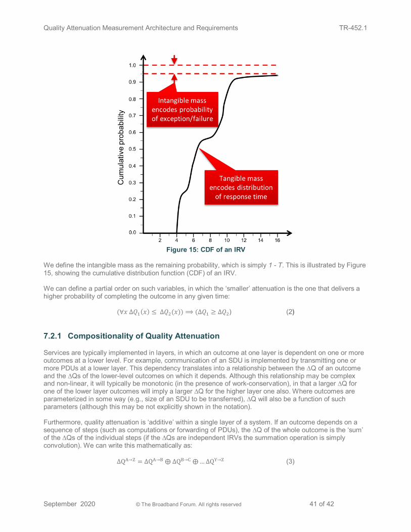
Quality Attenuation Measurement Architecture and Requirements TR-452.1
September 2020 © The Broadband Forum. All rights reserved 41 of 42
Figure 15: CDF of an IRV
We define the intangible mass as the remaining probability, which is simply 1 - T. This is illustrated by Figure 15, showing the cumulative distribution function (CDF) of an IRV. We can define a partial order on such variables, in which the ‘smaller’ attenuation is the one that delivers a higher probability of completing the outcome in any given time:
(∀𝑥𝑥 Δ𝑄𝑄1(𝑥𝑥) ≤ Δ𝑄𝑄2(𝑥𝑥)) ⟹ (Δ𝑄𝑄1 ≥ Δ𝑄𝑄2) (2)
7.2.1 Compositionality of Quality Attenuation
Services are typically implemented in layers, in which an outcome at one layer is dependent on one or more outcomes at a lower level. For example, communication of an SDU is implemented by transmitting one or more PDUs at a lower layer. This dependency translates into a relationship between the ∆Q of an outcome and the ∆Qs of the lower-level outcomes on which it depends. Although this relationship may be complex and non-linear, it will typically be monotonic (in the presence of work-conservation), in that a larger ∆Q for one of the lower layer outcomes will imply a larger ∆Q for the higher layer one also. Where outcomes are parameterized in some way (e.g., size of an SDU to be transferred), ∆Q will also be a function of such parameters (although this may be not explicitly shown in the notation). Furthermore, quality attenuation is ‘additive’ within a single layer of a system. If an outcome depends on a sequence of steps (such as computations or forwarding of PDUs), the ∆Q of the whole outcome is the ‘sum’ of the ∆Qs of the individual steps (if the ∆Qs are independent IRVs the summation operation is simply convolution). We can write this mathematically as:
∆QA→Z = ∆QA→B ⨁ ∆QB→C ⨁…∆QY→Z (3)
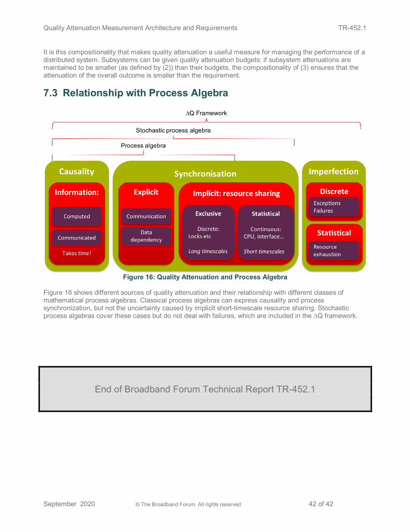
Quality Attenuation Measurement Architecture and Requirements TR-452.1
September 2020 © The Broadband Forum. All rights reserved 42 of 42
It is this compositionality that makes quality attenuation a useful measure for managing the performance of a distributed system. Subsystems can be given quality attenuation budgets; if subsystem attenuations are maintained to be smaller (as defined by (2)) than their budgets, the compositionality of (3) ensures that the attenuation of the overall outcome is smaller than the requirement.
7.3 Relationship with Process Algebra
Figure 16: Quality Attenuation and Process Algebra
Figure 16 shows different sources of quality attenuation and their relationship with different classes of mathematical process algebras. Classical process algebras can express causality and process synchronization, but not the uncertainty caused by implicit short-timescale resource sharing. Stochastic process algebras cover these cases but do not deal with failures, which are included in the ∆Q framework.
End of Broadband Forum Technical Report TR-452.1