Contents of the section:

Quantum thermal physics and some question of temperature

AN ATTEMPT AT QUANTUM THERMAL PHYSICS

J. J. Mareš and J. Šesták

Journal of Thermal Analysis and Calorimetry, Vol. 82 (2005) 681–686

RELATIVISTIC TRANSFORMATION OF TEMPERATURE AND MOSENGEIL–OTT’S ANTINOMY

J.J. Mareš, P. Hubík, J. Śesták, V. Śpička, J. Krištofik, J. Stávek

Physica E 42 (2010) 484–487

SHADOWS OVER THE SPEED OF LIGHT

J.J. Mareš, P. Hubík, V. Śpička, J. Stávek, J. Śesták, J. Krištofik

Phys. Scr. T151 (2012) 014080 (© The Royal Swedish Academy of Sciences)

PHENOMENOLOGICAL MEANING OF TEMPERATURE

Jiří J. Mareš

Chapter 2 in the book „Some Thermodynamic, Structural and Behavioural Aspects of Materials Accentuating Non-crystalline States” (J. Šesták, M. Holecek and J. Malek, editors),. OPS-ZCU Pilsen 2011, ISBN 978-80-87269-20-6.

Introduction

Motivation for this work were mainly informal discus-

sions at two conferences [1] concerning the validity of

the Second law of thermodynamics in case where the

quantum nature of the system must be taken into ac-

count. As we were in the past engaged in research into

practical problems requiring application of thermody-

namics to quantum systems [2–6], we feel ourselves in

the position to express our meaning also to the funda-

mental questions involved. Therefore, the main pur-

pose of this work is to express our opinion on these

questions and to present a sketch of an alternative con-

ceptual structure of quantum thermal physics rather

than to investigate a particular problem in detail. Our

subject should be, of course, distinguished from that of

quantum thermodynamics based on the consequent im-

plementation of quantum-mechanical concepts into

classical thermodynamics as is known from standard

literature (e.g. [1, 7]).

Besides analytical mechanics and theory of elec-

tromagnetic field, it is thermodynamics that is consid-

ered to be a well-established, logically closed theory.

There are even various axiomatic forms of the ther-

modynamics, which seem to guarantee absolute clear-

ness of concepts involved. In spite of that we have se-

rious difficulty in finding any book where the subject

is treated in a way really clear to an ordinary student.

As we are convinced, the very origin of the difficult

understanding of thermodynamics is connected just

with an inconvenient choice of conceptual basis more

than 150 years ago. Traditionally the most obscure is

an artificial concept of entropy and rather exceptional

form of the ‘Second law’ of thermodynamics.

Whereas the universal laws have mostly the form of

conservation laws, the logical structure of the Second

law is quite different. Ultimately formulated, it is a

law of irreparable waste of ‘something’ in every real

physical process. This imperative negativistic and

pessimistic nature of the Second law is very likely, for

philosophers but also for many active researches in

the field, the permanent source of dissatisfaction.

That is why the criticism aimed at the Second law has

the history as long as the Second law itself. Moreover,

in recent decade an unprecedented number of chal-

lenges have been raised against the Second law from

the position of quantum mechanics [1]. These argu-

ments, however, are as a rule, enormously compli-

cated with numerous approximations and neglects

and consequently rather questionable.

It is a very old empirical fact that the thermal

processes in the nature are submitted to certain re-

strictions strongly limiting the class of possible pro-

cesses. The exact and sufficiently general formulation

of these restrictions is extremely difficult and some-

times incorrect (cf. e.g. the principle of antiperistasis

[8], Braun-le Chatelier’s principle [9] and Second

law) but in spite of it very useful. That is why the au-

thors of this paper believe that the Second law (or an-

other law which puts analogous limitations on ther-

mal processes) does reflect experimental facts with an

appreciable accuracy and thus it should be incorpo-

rated into the formalism of thermodynamics. On the

other side, being aware of the fact that the contempo-

rary structure of thermodynamics with its rigid con-

ceptual basis may have intrinsic flaws, we claim that

the absolute status of the Second law should not be

criticized or denied from the point of view of another

physical theory (e.g. quantum mechanics) prior the

correction of these imperfections has been made.

1388–6150/$20.00 Akadémiai Kiadó, Budapest, Hungary

© 2005 Akadémiai Kiadó, Budapest Springer, Dordrecht, The Netherlands

Journal of Thermal Analysis and Calorimetry, Vol. 82 (2005) 681–686

AN ATTEMPT AT QUANTUM THERMAL PHYSICS

J. J. Mareš* and J. Šesták

Institute of Physics, Academy of Sciences of the Czech Republic, Cukrovarnická 10, CZ-162 53 Praha 6, Czech Republic

This paper outlines an alternative exposition of the structure of quantum thermodynamics which is essentially based on Carnot’s

theory where fluxes of caloric are identified with negative information fluxes. It is further assumed that the thermal energy evolved

by thermal processes is identical with the electromagnetic zero-point background energy evolved by the destruction of information

inscribed in a structural unit (qubit). Theoretical arguments on an elementary level are accompanied by illustrative examples.

Keywords: caloric, entropy, information, quantum thermodynamics, zero-point radiation

* Author for correspondence: semicon@fzu.cz

Reformulation of fundamental laws ofthermodynamics

A serious flaw in the conceptual basis of classical

thermodynamics concerns even the so-called First

law of thermodynamics. The first step toward this law

was made by Benjamin Count of Rumford by the gen-

eralisation of his observations made at an arsenal in

Munich (1789) [10]. Accordingly, practically unlim-

ited quantity of heat was possible to produce only by

mechanical action i.e. by boring of cannon barrels by

a blunt tool and this experimental fact was by

Rumford analysed as follows: ‘It is hardly necessary

to add, that any thing which any insulated body, or

system of bodies, can continue to furnish without lim-

itations, cannot possibly be a material substance: and

it appears to me extremely difficult, if not quite im-

possible, to form any distinct idea of anything, capa-

ble of being excited and communicated, in the manner

the heat was excited and communicated in these ex-

periments, except it be motion’. The same idea that

heat absorbed by a body, which is particularly respon-

sible e. g. for the increase of its temperature, is identi-

cal with the kinetic energy of its invisible components

was further apparently supported by arguments due to

J. P. Joule [11]. Results of his ingenious and marvel-

lously accurate experiments have been summarized

into two points: The quantity of heat produced by the

friction of bodies, whether solid or liquid is always

proportional to the quantity of force expended. The

quantity of heat capable of increasing the temperature

of a pound of water by 1° Fahrenheit requires for its

evolution expenditure of a mechanical force repre-

sented by the fall of 772 lbs. through the space of one

foot (here the term ‘force’ has evidently meaning of

energy). In spite of clearness of these correct state-

ments, Joule did not stressed out explicitly the fact

that in his experiment we have to do only with

one-way transformation of work into the heat. Instead

he tacitly treated throughout the paper the heat as it

were a physical entity fully equivalent or identical

with mechanical energy. It was probably due either to

influence of Rumford or to the reasoning that in the

experiment heat appears just when mechanical work

disappears and ipso facto these two entities must be

identical. Such an extremely suggestive but incorrect

idea was later canonized by Clausius [12] who

proclaims an object of thermodynamics to be ‘die Art

der Bewegung, die wir Wärme nennen’ i.e. the kind

of motion we call heat.

In the history of thermodynamics objections ap-

peared against such an energetic interpretation of the

heat. Unfortunately, these objections were only rare and

with no adequate response. One of them is due e.g. to

Mach [13]. Accordingly, it is quite easy to realize device

of Joule’s type where a given amount of energy W is

completely dissipated and simultaneously the heat in

amount Q=JW is evolved, where J is universal Joule’s

proportionality factor. On the other side, as far as it is

known, there is no single real case where the same

amount of heat Q is transformed back into mechanical

work W=Q/J only by reversion the original process.

Taking into account this circumstance together with the

very generic property of the energy, which can be prin-

cipally converted into another form of energy without

any limitation, we must exclude the logical possibility

that the heat is energy at all. Of course, postulating the

equivalence of energy and heat a meaningful mathemat-

ical theory of thermal processes can be and actually has

been established. The price paid for the equivalence

principle is, however, rather high. In order to make the

theory consistent it was necessary to create somewhat

artificial and highly abstract quantities like entropy,

enthalpy, free energy, and various thermodynamic po-

tentials the meaning of which is more formal than physi-

cal. The mathematical manipulations with their ~720

derivatives and differentials (which are sometimes total)

[14] actually do provide results the interpretation of

which is, however, rather matter of art than of science.

Heat as an Entropy–Caloric

Astonishingly an elegant way leading out from these

problems was very likely for the first time suggested

by Callendar [15] and later in more sophisticated

form worked out by Job in his impressive book [16].

The main idea is that the heat in common sense (e.g.

as a cause of elevation of temperature of bodies ex-

posed to the heating) should not be identified with a

kind of energy but with the entropy, which is known

from classical thermodynamics. It was shown by Lar-

mor [17] and especially by Lynn [18] in a very preg-

nant way that the heat could be measured in energy

and entropy units as well. In the latter case the

heat–entropy concept attains the content identical

with the concept of Carnot’s ‘caloric’ � [19], whereas

the empirical temperature �, i.e. ‘hotness’ [13], auto-

matically starts to play the role of its potential. (We

are using for caloric Greek final letter � as this letter

involves both, usual S for entropy and C for caloric.)

For the increase of potential energy d� of the amount

of caloric � due to the increase of temperature by d�

we may, namely, write:

d d� � � �� �F ( ) (1)

where F’(�) is so-called Carnot’s function. It is an ex-

perimental fact that this function can be reduced to the

universal constant = 1 using instead of arbitrary empiri-

cal temperature scale � the ideal gas temperature scale Tequivalent to the absolute Kelvin scale [20, 21]. (Notice

that Carnot’s function in (1) corresponds to the situation

682 J. Therm. Anal. Cal., 82, 2005

MAREŠ, ŠESTÁK

where the heat is measured in entropy and not in energy

units [22]). In this case for the potential energy � corre-

sponding to the given amount of caloric � kept at the

temperature T we can write:

� �� T (2)

The perfect analogy with other potentials known

from physics, such as gravitational and electrostatic

potentials, is then evident. After the terminological

substitution of heat-energy by heat-entropy it is only a

technical problem to reformulate two fundamental

laws in a manner which is common in classical axi-

omatic thermodynamics [23], namely:

I.) Energy is conserved in any real thermal process

II.) Caloric (heat) cannot be annihilated in any

real thermal process

Notice that the first and second law, formulated in

such a way are conceptually disjunctive because calo-

ric has nothing to do with energy. The possible link

between these laws and quantities, however, provides

formula (2). We shall not discuss here application of

theorem II) to particular cases known from empirical

observations of real processes (it is already done e.g.

in [16]) but, instead, we proceed further making use

of an important relation existing between entropy and

information. It was recognized by Szilárd in his pio-

neering work [24] that in a certain thermal process the

exchange of information must play an essential role.

Afterwards, the establishment of fundamentals of in-

formation theory [25] enabled Brillouin to reformu-

late this idea with an appreciable mathematical rigor

[26]. (For more recent review on the information-en-

tropy relation, see e.g. [27].) Accordingly, the infor-

mation � has a character of negative entropy (i.e. we

are allowed to write �= –�) and therefore, in our

old-new provisional terminology, we can identify the

production of caloric with the destruction of informa-

tion and the flux of caloric with the information flux

in an opposite direction. Theorem II) can thus be re-

formulated in terms of information as:

II*) Information (�) is destroyed in any real ther-

mal process

Veracity of this theorem seems to be very obvious at

first glance. Indeed, almost everybody has experience

that by combustion of newspapers in a stove or petrol

in a car engine these materials are lost forever, to-

gether with the information involved. On the other

hand, it is little convincing that such a ‘tiny thing’ as

the information is, can really be able to control natural

thermal processes. Isn’t it more likely that state-

ment II*) concerns only side effects taking place in

certain cases? We do not think so and we assume that

the validity of postulate II*) is quite general and apt

for substitution of the Second law of thermodynam-

ics. Moreover, besides the properties of the caloric al-

ready discussed, just the existence of the direct link

between caloric (i.e. heat) and information is the very

reason for which we prefer to use for the quantum de-

scription of thermal processes rather the conceptual

basis of caloric theory than that of classical thermody-

namics. In conclusion of this paragraph and as illus-

tration of such an approach, let us paraphrase

Rumford’s original analysis of his experiments cited

above by simply writing there instead of the word

‘motion’ the phrase ‘perished information’.

Quantum nature of information bound to caloric

In order to involve the information into the physical

reasoning it is convenient to convert information

coded, as usual, in binary units �2 (bits) into the infor-

mation �p expressed in physical units. This relation

obviously reads:

�p=(kln2)�2 (3)

where k is Boltzmann’s constant (k =1.38·10–23 J K–1).

It should be stressed here that by choosing

Boltzmann’s constant as a conversion factor simulta-

neously the absolute Kelvin scale was chosen for tem-

perature measurements.

We assume now that there is no information ‘an

sich’ or in other words information needs in all cases

a material carrier. From the point of view of macro-

scopic thermal physics there is, however, fundamen-

tal difference between e.g. genetic information in-

scribed in the DNA and information provided by a

gravestone inscribed with personal data. Whereas in

the former case for coding of information structural

units on molecular level are used, which should be de-

scribed by microscopic many-body formalism, to the

later case rather a macroscopic description in terms of

boundary–value problem is adequate. To distinguish

without ambiguity between these two extreme cases

we need, however, a criterion which, having a sign of

universality specifies what the ‘molecular level is’.

As far as we know, a good candidate for such a crite-

rion is modified Sommerfeld’s condition

distinguishing between classical and quantum effects

[28, 29]. It reads:

� � 2� (4)

where � is phase space occupied by a structural unit

(‘qubit’) where minimally 1 bit information is stored

and � is the Planck’s universal constant

(�=1.05·10–34 Js). Direct computation of the action �

corresponding to one atom built in an ordinary crys-

tal, liquid or gas confirms the validity of condition (4)

in these cases. It proves the fact that every atom to-

gether with its nearest neighbourhood should be

treated as a quantum structural unit responsible for in-

J. Therm. Anal. Cal., 82, 2005 683

AN ATTEMPT AT QUANTUM THERMAL PHYSICS

formation storage on a ‘molecular level’. Generaliz-

ing this result, we can conclude that the very nature of

Carnot’s caloric is the destructed information origi-

nally coded in occupied quantum states of structural

units of which the macroscopic system under investi-

gation consists.

Inexhaustible source of energy for thermal processes

The mechanism of information transfer through the

macroscopic system is assumed to be due to erasing

information in one particular structural unit which is

influenced by the neighbouring one in the field of

long range forces defined by macroscopic system as a

whole. There are, however, limitations of such a pro-

cess. First, as the information storage in both neigh-

bouring structural units is submitted to the same con-

dition (4) it is impossible to exchange more

information from one unit to another than ~1 bit per

2� of the occupied phase space. Second, the ex-

change of information must be in agreement with

boundary conditions put on the macroscopic system

as a whole, which are locally realized e.g. by long

range forces. It may thus happen that the transfer of

some information from one unit to the neighbouring

unit is incompatible with these external conditions

and information is lost. The loss of information physi-

cally means that some characteristic pattern of struc-

tural unit has disappeared and a wider class of quan-

tum states becomes accessible. In the frame of the

presented model any loss of information should be ac-

companied with the development of energy. How to

explain where the energy comes from?

We are inclined to interpret the stability of quan-

tum objects as a result of existence of zero-point elec-

tromagnetic vacuum fluctuations exactly compensat-

ing energy loses due to the recoil radiation from this

object. Such an approach well known from stochastic

and quantum electrodynamics [30, 31], confines our

considerations to the systems controlled only by elec-

tromagnetic interactions, namely, low temperature

plasma, gases, condensed matter and chemical reac-

tions in these systems. Accordingly, the cohesion en-

ergy of any such a system is nothing but the energy of

electromagnetic modes of the background zero-point

radiation accommodated in such a way that they fit

the geometry of the system. Characterizing the di-

mensions of the quantum electromagnetic system (for

which the universal constants � and c must be taken

into consideration) by a single length parameter a, we

immediately obtain for cohesion energy a formula of

Casimir’s type by applying dimensional analysis [32]:

� � ( / )�c a (5)

where the dimensionless parameter should be deter-

mined from a particular geometry of the system (usually

ranges from 0.1–0.001 [30]). The change of dimension

a or complete destruction of a structural unit with en-

ergy (5) during thermal process has a consequence that

just this amount of energy is developed at the place. As

this energy is in fact a modified energy of all-pervasive

universal zero-point background, we have to do with an

energy supply from practically inexhaustible non-local

source of energy. Therefore, within the frame of sto-

chastic electrodynamics every thermodynamic quantum

system should be interpreted as an open system even in

the case where it is finite.

Examples

In order to make the presented system of quantum

thermodynamics more intelligible we have given

three examples illustrating how should be some com-

mon observations within the frame of this system

interpreted.

1) How does the heat engine work? Heat engine

in the sense of original Carnot’s theory is nothing but

a kind of mill driven by caloric � falling from a higher

potential T1 (boiler) to a lower potential T2 (cooler).

Information thus flows from the cooler with con-

densed water (better ordered than steam) to the cylin-

der of engine where the information is destroyed (by

weakening of correlations among molecules during

the expansion) giving rise to useful work originating

in zero-point background. Then the residual informa-

tion continues to flow to the heater where it is dis-

solved during ordering of configuration of the steam.

Notice that the flow of information and the flow of

water are just opposite in this case and that the ques-

tion how the boiler is heated is put aside. In a typical

combustion engine at low temperature the fuel with

high information content flows into the cylinder of

engine. During the combustion of fuel the informa-

tion which is coded in its structure is destroyed and

the useful work from the zero-point quantum electro-

magnetic energy is produced there. The information,

however, flows inside the combustion space for this

type of engine also through the exhaust-pipe so that

special attention must be paid to this part.

2) There is an interesting device called Bunsen’s

ice calorimeter. As this apparatus works at a well de-

fined temperature TM (i.e. melting temperature of ice

=273 K) it, in fact, according to equation (2), mea-

sures directly inputted caloric and may thus serve as

‘entropymeter’. Indeed, the information destroyed

and the latent energy of melting is connected here in

an especially obvious way. An estimate of the latent

energy �M per one mol of ice can be obtained as fol-

lows. We make a use of an important fact that the H2O

684 J. Therm. Anal. Cal., 82, 2005

MAREŠ, ŠESTÁK

molecules retain their integrity in both water and ice,

simultaneously neglecting the effect of clustering of

molecules at temperatures well above the melting

point which is responsible for non-trivial macro-

scopic behaviour of water [33, 34]. Within the frame

of such a simplified model it would be then necessary

for the melting of ice to break down 4 well-oriented

bonds per every water molecule and substitute them

by quasi-continuum of states. Such a transformation

corresponds approximately to the destruction of �2=4

bits of information per molecule [27]. Taking into ac-

count equations (2) and (3) we can thus write:

� M MNk T� ( ln )2 �� (6)

where N is Avogadro’s constant (N=6.02·1023 mol–1).

The estimate of �M then reads �6288 J mol–1 in an ex-

cellent agreement with the experimental value

=6007 J mol–1.

3) There are different microscopic parameters

characterizing the configuration of a structural unit

where the information is stored which can be in prin-

ciple constructed from quantum numbers describing

this system. The relation connecting these micro-

scopic parameters and macroscopic boundary condi-

tions is evidently very complicated. If we, however,

as above, confine ourselves only to a single parameter

a – characteristic dimension of the structural unit, this

relation can be found in an explicit form and com-

pared directly with experimental data. Combining

formulae (2) and (3) the temperature change of the

potential energy of a structural unit which is due to

the erasing of information �2 from it is given by:

d d� / ( ln )T k� 2 �2 (7)

Substituting for � the Casimir’s quantum cohe-

sion energy (5) we immediately obtain an estimate for

the corresponding relative expansion of the unit:

d dln / ( ln / )a T a k c� 2 � �2 (8)

Assuming that the thermal process is homoge-

neous and isotropic, this coefficient must be within

the order of magnitude identical with the expansion

coefficient macroscopically observed. For typical

condensed matter where bond length a�4·10–10 m and

�2=1 we obtain from (8) for coefficient of relative

thermal expansion a value of 1.2·10–7/ which is near

to the values experimentally observed (typically

�10–5), provided that �0.01.

Conclusions

In conclusion, using elementary arguments without

mathematical rigor, changes in the conceptual basis

and in the structure of quantum thermodynamics have

been suggested. The resulting theory is based essen-

tially on the following points:

• Modified form of Carnot’s theory where caloric is

identified with the entropy.

• Equivalence of information and negative entropy.

• Interpretation of stability of quantum objects as the

consequence of the existence of electromagnetic

zero-point vacuum radiation.

The authors are aware that the structure of quan-

tum thermodynamics as sketched out in this paper is

far from to be mature, however, they are simulta-

neously convinced that it is potentially apt to reflect

the empirical facts in a more intelligible way than the

present theories.

Acknowledgements

This work has been supported by the Grant Agencies of the

Czech Republic and of the Academy of Sciences (Projects Nos

202/03/0410 and 522/04/0384).

References

1 1st IC on Quantum limits to the Second law, San Diego

‘02, Ed. D. P. Sheehan, AIP Proceedings, 643 (AIP, Mel-

ville, 2002), see also Proc. of 2nd IC on Frontiers of

Mesoscopic and Quantum Thermodynamics, Prague 2004,

Ed. V. Špi�ka.

2 J. Šesták, J. Therm. Anal. Cal., 69 (2002) 1113.

3 Z. Kalva and J. Šesták, J. Therm. Anal. Cal., 76 (2004) 67.

4 B. Hlavá�ek, J. Šesták and J. J. Mareš, J. Therm. Anal.

Cal., 67 (2002) 239.

5 J. Strnad, J. Protivínský, Z. Strnad, A. Helebrant and

J. Šesták, J. Therm. Anal. Cal., 76 (2004) 17.

6 J. J. Mareš, J. Stávek and J. Šesták, J. Chem. Phys.,

121 (2004) 1499.

7 T. Feldmann and R. Kosloff, Phys. Rev., E 68 (2003)

016101.

8 K. Meyer-Bjerrum, Die Entwicklung des Temperaturbegriffs

im Laufe der Zeiten (Vieweg u. Sohn, Braunschweig, 1913).

9 P. Ehrenfest, Journ. D. Russ. Phys. Ges., 41 (1909) 347 (in

Russian).

10 Count Rumford, Phil. Trans., 88 (1789) 80.

11 J. P. Joule, Phil. Trans., 140 (1850) 61.

12 R. Clausius, Mechanische Wärmetheorie, (Vieweg u.

Sohn, Braunschweig, 1876).

13 E. Mach, Die Principien der Wärmelehre (Verlag von

J. A. Barth, Leipzig, 1896)

14 P. W. Bridgman, The Nature of Thermodynamics (Har-

vard University Press, Cambridge, 1941).

15 H. L. Callendar, Proc. Phys. Soc. of London, 23 (1911) 153.

16 G. Job, Neudarstellung der Wärmelehre – Die Entropie als

Wärme, (Akad. Verlagsges., Frankfurt am Main, 1972).

17 J. Larmor, Proc. Royal Soc. London, A 194 (1918) 326.

18 A. C. Lynn, Phys. Rev., 14 (1919) 1.

19 S. Carnot, Réflexions sur la puissance motrice du feu,

(Bachelier, Paris, 1824).

J. Therm. Anal. Cal., 82, 2005 685

AN ATTEMPT AT QUANTUM THERMAL PHYSICS

20 J. J. Mareš, J. Therm. Anal. Cal., 60 (2000) 1081.

21 W. Thompson (Lord Kelvin),Trans. Royal Soc.

Edinburgh, 16 (1849) 541.

22 H. T. Wensel, J. Appl. Phys. 11 (1940) 373.

23 C. Truesdell, Rational Thermodynamics (McGraw-Hill,

New York, 1969)

24 L. Szilárd, Z. F. Physik, 53 (1929) 840.

25 C. E. Shannon, Bell Syst. Techn. J., 27 (1948) 379, 623.

26 L. Brillouin, J. Appl. Phys., 24 (1953) 1152.

27 A. Wehrl, Rev. Mod. Phys., 50 (1978) 221.

28 A. Sommerfeld, Phys. Z., 24 (1911) 1062.

29 J.-M. Lévy-Leblond and F. Balibar, Quantics, Rudiments

of Quantum Physics (North-Holland, Amsterdam,1990).

30 L. de la Pe�a and A. M. Cetto, The Quantum Dice – An

Introduction to Stochastic Electrodynamics (Kluwer Aca-

demic Publishers, Dordrecht, 1996).

31 P. W. Milloni, The Quantum Vacuum – An Introduction to

Quantum Electrodynamics (Academic Press Inc., Boston,

1994).

32 J. Palacios, Dimensional Analysis (MacMillan and Comp.,

Ltd., London, 1964).

33 J. D. Bernal and R. H. Fowller, J. Chem. Phys., 1 (1933) 515.

34 L. Pauling, J. Am. Chem. Soc., 57 (1935) 268.

DOI: 10.1007/s10973-005-6886-2

686 J. Therm. Anal. Cal., 82, 2005

MAREŠ, ŠESTÁK

ARTICLE IN PRESS

Physica E 42 (2010) 484–487

Contents lists available at ScienceDirect

Physica E

1386-94

doi:10.1

� Corr

E-m

journal homepage: www.elsevier.com/locate/physe

Relativistic transformation of temperature and Mosengeil–Ott’s antinomy

J.J. Mares �, P. Hubık, J. Sest�ak, V. Spicka, J. Kristofik, J. St�avek

Institute of Physics of the ASCR, v. v. i., Cukrovarnick �a 10, 162 00 Prague 6, Czech Republic

a r t i c l e i n f o

Available online 24 June 2009

Keywords:

Phenomenological temperature

Lorentz’s transformation

Hotness manifold

Thermoscopy

77/$ - see front matter & 2009 Elsevier B.V. A

016/j.physe.2009.06.038

esponding author. Fax: +420 23343184.

ail address: maresjj@fzu.cz (J.J. Mares).

a b s t r a c t

A not satisfactorily solved problem of relativistic transformation of temperature playing the decisive

role in relativistic thermal physics and cosmology is reopened. It is shown that the origin of the so-

called Mosengeil–Ott’s antinomy and other aligned paradoxes are related to the wrong understanding of

the physical meaning of temperature and application of Planck’s Ansatz of Lorentz’s invariance of

entropy. In the contribution, we have thus reintroduced and anew analyzed fundamental concepts of

hotness manifold, fixed thermometric points and temperature. Finally, on the basis of phenomen-

ological arguments the Lorentz invariance of temperature and relativistic transformations of entropy are

established.

& 2009 Elsevier B.V. All rights reserved.

1. Introduction

There is a non-trivial problem connected with the relativistictransformation of temperature which can be, however, reduced toa simple question: is the body moving with the velocity v

relatively to the rest system of coordinates in its own coordinatesystem colder or hotter than if it were measured in the rest systemof coordinates? Very early after the appearance of the specialtheory of relativity in 1905 the problem was solved by a pupil ofvon Laue, von Mosengeil, who provided the following result [1]:

T ¼ T0

ffiffiffiffiffiffiffiffiffiffiffiffiffiffiffiffiffiffiffiffiffiffiffiffið1� v2=c2Þ

q; ðMosengeil; 1907Þ ð1Þ

where T0 is the Kelvin temperature as measured in the rest systemof coordinates and T the corresponding temperature detected inthe moving system. The satisfaction with this formula which is upto now serving as a standard in textbooks on special theory ofrelativity was put in doubts by a challenging paper due to Ott [2]where just an inverse formula for the relativistic transformation oftemperature is derived, namely

T ¼ T0=ffiffiffiffiffiffiffiffiffiffiffiffiffiffiffiffiffiffiffiffiffiffiffiffið1� v2=c2Þ

q: ðOtt; 1963Þ ð2Þ

After the appearance of Ott’s paper a vivid discussion in‘‘Nature’’ [3–8] broke out which, however, stopped after sometime without bringing any clear decision which of these twoformulae is true [9,10]. At the end of the 20th century, during thelast wave of interest in the problem [11,12], however, another

ll rights reserved.

opinion appeared, namely that the temperature must be Lorentzinvariant [13].

As we believe for the solution of this fundamental problem ofrelativistic thermal physics, it is inevitable to first make it clearwhat the temperature actually is and what it is not. Therefore,before suggesting our solution of this interesting puzzle, we arecritically revising the definition of fundamental concept ofphenomenological thermal physics, i.e. that of the temperature.

2. The concept of temperature

Astonishingly, a satisfying definition of the phenomenologicalphysical quantity called temperature is lacking in the literature.There exist, of course, definitions in terms of statistical physics,which are, however, related to the phenomenological quantitymeasured by a macroscopic device, thermometer, only by rathersuperficial considerations. Taking further into account thatpractically all actual temperature measurements are performedby means of thermometers and not by statistical analysis ofbodies, treated as statistical ensembles of elementary particlesand excitations, an urgent need for a good phenomenologicaldefinition of temperature is thus evident.

It should be stressed here that the temperature is not aprimary concept but, as was for the first time with sufficientplausibility shown by Mach [14], that the nearest experimentallyaccessible structure behind is so-called hotness manifold (‘‘Man-nigfaltigkeit der Warmezustande’’) the elements of which arehotness levels which are one-to-one related with experimentallyobservable thermoscopic states. As was shown in our recentpaper [15], the existence of such a set of thermoscopic states maybe proved using an operational definition specifying the proper-ties of a measuring device (thermoscope) together with the

ARTICLE IN PRESS

J.J. Mares et al. / Physica E 42 (2010) 484–487 485

measurement conditions. The most salient among these condi-tions is that of thermal equilibrium [16] that is enabled by athermal (diathermic) contact of the thermoscope with a bodyunder investigation and the existence of which may be checkedindependently by so-called correlation test.1 It is an importantconsequence of the introduction of thermoscopes that we canexperimentally observe the topological order of hotness levels asan order of quite another real physical quantity called thermo-scopic variable (e.g. length of mercury thread, resistance andthermoelectric voltage). As these thermoscopic variables are realcontinuous quantities defined in certain closed intervals, thisproperty is transferred by the said one-to-one relation also intothe hotness manifold. The sewing-up of the different sets ofthermoscopic states corresponding to the different thermoscopicvariables, however, was shown not to be possible withoutexploitation of another physical entity, fixed (thermometric)points. The fixed point is a body prepared according to a definiteprescription for which it is known that the thermoscope indiathermic contact with this body indicates reproducibly the well-defined thermoscopic state. The fixed points such as boiling pointof helium, melting point of water, boiling point of water, andmelting point of platinum (all at normal atmospheric pressure)are examples well-known from practical thermometry [17].Because of the correspondence between the fixed points andsome of thermoscopic states, the set of fixed points is ordered and,because fixed points are real bodies, countable. Furthermore, animportant empirical fact that the limitations put on theconstruction of the fixed points are not known2 makes plausiblethe assumption that for each fixed point there is another ‘‘hotter’’or another ‘‘colder’’ one and that there is an inter-lying fixed pointbetween any two fixed points, sounds quite reasonably. Just such aproperty enables one not only to sew-up together the differentoverlapping parts of the hotness manifold corresponding tovarious thermoscopic variables but simultaneously provides adense countable subset in the hotness manifold ensuring that thisset is linear [18], and thus fully equivalent to the set of the realnumbers (real axis).

Now we are ready to approach to the following definition:temperature is any continuous one-to-one order-preservingmapping of hotness manifold on a simply connected subset ofreal numbers. It is evident from this definition that we have anenormous liberty to choose a particular temperature scale whichthus rests entirely upon a convention. Only the hotness formallyrepresented by hotness manifold has a right to be regarded as anentity existing in the Nature (cf. [14]). From this point of view ourquestion, i.e. how the temperature, which is in fact a result ofsome arbitrary mapping, behaves by relativistic transformations,sounds as an ill-defined assignment. Indeed, the solution of theproblem will depend on the particular way how the temperatureis constructed and not only on the objective constraints. Moreover,it is quite clear that the rationality or irrationality of choice of thetemperature scale will be decisive for further performance and

1 A correlation test is the procedure frequently used in practical thermometry

which can be in general terms described as follows. Let us have in an inertial frame

two systems, A and B, separated by a macroscopically firm material partition

defining their common boundary. Such a partition is called diathermic if the

changes of system A induce the changes of system B and vice versa.2 The temperatures observed range from �10�10 K (Low Temperature Lab,

Helsinki University of Technology) up to�109 K (supernova explosion) without any

traces that the ultimate limits were actually reached. Speculative upper limit

provides only the so-called Planck temperature TP ¼ O(_c/G)� (c2/

k)E1.417�10321K, hypothetically corresponding to the first instant of Big Bang

and depending on the assumption that the constants involved are really universal.

Therefore, the conjecture presented in this paper, i.e. that the hotness manifold has

no upper or lower bound, is obviously valid at least for all phenomena already

known.

intelligibility of theory of thermal effects. Therefore, for thesolution of our problem a detailed analysis of temperatureconcept in use is quite essential.

On the more-or-less historical and practical grounds, in otherwords, on the basis of fully arbitrary anthropomorphic criteria[15], a special mapping of the hotness manifold was chosen on anordered subset of real numbers called the ideal (perfect) gas scale.The equation controlling the behavior of the ideal gas, which is ahypothetical substance or concept rather than a real thing, reads

pV ¼ nRT ; ð3Þ

where p and V are, respectively, the pressure and the volume ofthe ideal gas which alternatively play the role of thermoscopicvariables. As the hypothetical thermoscope is considered aconventional gas thermometer [19] filled with n moles, n40, ofideal gas. The constant R on the right side of Eq. (3), which neednot be Lorentz invariant, has then a form of product R ¼ kN wherek and N are Boltzmann’s and Avogadro’s constants, respectively.The ideal gas temperature scale T defined by means of Eq. (3) hassome remarkable properties. For example, as both quantities p

and V have a natural lower bound ¼ 0, the temperature T has alsothis lower bound and thus belongs to the class of absolutetemperatures [20] for which one assumes that always T40.Notice that the possible value T ¼ 0 is already excluded by ourdefinition of temperature, because due to the absence of thelowest hotness level in the hotness manifold any continuous one-to-one order-preserving transformation has inevitably to map itsimproper point (i.e. �N) just on the point corresponding toabsolute zero. Nernst’s law of unattainability of absolute zero oftemperature [21] is thus together with its consequences intrinsi-cally involved in this definition of temperature.

3. Lorentz transformation of temperature

Already having at our disposal the prescription defining thetemperature in mathematical terms, it is in principle possible toperform the Lorentz transformation of the left-hand side of Eq. (3)and to obtain in this way the formula for the relativistictransformation of temperature. The physical reasoning behindsuch a computation would not be, however, very transparent andconvincing because the gas thermometer is rather a difficultdevice. Moreover, in order to be able to also analyze othertemperature measuring methods (using e.g. platinum resistance,black-body radiation and thermoelectric voltage) in a sufficientgenerality the methodical approach is more relevant.

Fortunately, the properties of hotness manifold enable one tomake the following fairly general considerations. First of all, it isevident that in order to not to violate the principle of relativity thebehavior of bodies realizing fixed thermometric points has to bethe same in all inertial frames (cf. [22]). For example, it would beabsurd to admit an idea that the water violently boiling in its restsystem can simultaneously3 look calm if observed from anotherrelatively moving inertial system. In other words, any fixed pointhas to correspond to the same hotness level regardless of theinertial frame used for the observation. Assigning, by means ofsome convention, to each body realizing the fixed point a certain‘‘inventory entry’’, the resulting, by pure convention establishedlist of numbers cannot be changed by a mere transfer from oneinertial system to another.

3 Notice that we have to do here with the essentially time-independent

stationary process, where the Lorentz transformation of time plays no role. Let us

also recall that the pressure, controlling e.g. boiling point of water, may be proved

independently to be Lorentz invariant [23].

ARTICLE IN PRESS

J.J. Mares et al. / Physica E 42 (2010) 484–487486

For example, using, thus, as an operational rule for stocktakingof fixed points formula (3) (in SI units with R ¼ 8.3145 J/K mol)and assigning to the triple point of water an inventory entry273.16 K, we obtain an ordered table of fiducial points of ideal gasscale (similar to the ITS [17]) which must be valid in all inertialframes. As the set of fixed points provides a dense subset(skeleton) in continuous hotness manifold, such a Lorentz-invariant table can be extended and detailed as we like andconsequently, any hotness level can be, by means of this table,approximated with arbitrary accuracy. Due to the continuity ofprescription (3) the whole ideal gas (Kelvin) scale T is theninevitably Lorentz invariant.

The invariance of Kelvin scale has, however, a very interestingand far reaching consequence. Let us make the following‘‘Gedankenexperiment’’ with two identically arranged gasthermometers both filled with one mole of ideal gas which arein two relatively moving inertial systems in diathermic contactwith the same fixed point bath (for definiteness, with triplepoint of water) placed in their own frames. The pressure in bothdevices must be the same, because, as can be proved quiteindependently the pressure is Lorentz invariant [23]. Therefore,we can write

p ¼ p0; ð4Þ

T ¼ T0; ð5Þ

where index 0 is related, as above, to the quantities measured inthe a-priori chosen rest system. Taking now the well-knownLorentz transformation of volume into account, we obtain fromEq. (3) the following series of equations:

pV ¼ p0V0

ffiffiffiffiffiffiffiffiffiffiffiffiffiffiffiffiffiffiffiffiffiffiffiffið1� v2=c2Þ

q¼ RT ¼ R0T0

ffiffiffiffiffiffiffiffiffiffiffiffiffiffiffiffiffiffiffiffiffiffiffiffiffið1� v2=c2Þ;

qð6Þ

from which a somewhat astonishing relation immediatelyfollows:

R ¼ R0

ffiffiffiffiffiffiffiffiffiffiffiffiffiffiffiffiffiffiffiffiffiffiffiffiffið1� v2=c2Þ:

qð7Þ

The physical meaning of this formula is really far reaching.Taking into account, namely, that R is an entropy unit, Eq. (7) mustsimultaneously represent the transformation formula for entropyin general. This is, however, in severe contradiction with Planck’sAnsatz claiming that the entropy is Lorentz invariant. We have torecall here that this Ansatz, serving as a starting point ofnumerous considerations in relativistic thermodynamics, hasnever been proved with sufficient exactness but from thebeginning it was mere an intuitive conjecture [24]. (It was namelyargued that the entropy has to be invariant, because it is thelogarithm of a discrete number of states which is ‘‘naturally’’Lorentz invariant.) Nevertheless, admitting once the relativisticinvariance of temperature, we have to reject Planck’s conjecture asunsound and particularly, we can also no more treat the variousunits of entropy, e.g. gas constant R and Boltzmann’s constant k, asuniversal constants.

4 Interestingly enough, the similar assumption that the temperature measure-

ment is possible just only if the thermometer is in rest with respect to the

measured system is as self-evident, without any proof, used in the recent

theoretical literature, see e.g. [26].

4. Distant measurement of temperature

The very task of the special theory of relativity is to study thetransformation laws connecting the experimental results ofobservers in different inertial systems performing the samemeasuring operations. Frequent types of such measurements areso-called ‘‘distant measurements’’ the aim of which is todetermine the physical quantity belonging to a certain movinginertial system by means of measurements made at the restsystem. The operational methods for distant measurement of e.g.

length, time, and intensity of fields are generally known. In case oftemperature, however, due to its special physical nature weencounter some peculiar difficulties. The main problem, which isintuitively not quite obvious, is the principal impossibility toestablish the thermal equilibrium between two relatively movinginertial systems. Namely, the relative movement of systems A andB (see footnote 1) prevents one from answering withoutambiguity, on the basis of correlation test, the question whetherthe common boundary is diathermic or not, which makes anyjudgment on the thermal equilibrium quite questionable. Indeed,it is clear that the boundary between two relatively movingsystems has to move at least with respect to one of them. In such acase, however, the interaction between these systems can existeven if the boundary is non-diathermic (adiabatic). For example,the moving boundary can exert a pressure on one of the systemswithout changing the state of the other and/or a charged system Asurrounded by a metallic envelope, regardless of the fact whetherit is diathermic or adiabatic, can induce dissipative equalizationcurrents in system B without affecting the charge distributioninside system A. In order to exclude such cases, the temperature ofany body must be measured only by means of a thermometerwhich is in the rest with respect to the body, and this operationcannot be, in principle, performed by a relatively movingobserver4 (cf. also [25]). Hence the temperature cannot be thesubject of a direct distant measurement in principle. It can only bethe result of local measurement and subsequent data transfer intoanother inertial system. (If possible, the digital mailing of the datawould be the best choice.) Of course, as the theoretical basis forthe determination of temperature of moving objects Eq. (5),expressing the Lorentz invariance of temperature, has to besimultaneously taken into account. The operational rules fordistant measurement of temperature may then be formulated asfollows:

(1)

Bring the measured body in diathermic contact with thethermometer in their common inertial rest frame.

(2)

Reconstruct in the relatively moving inertial system thereading of the thermometer applying transformation rulesrelevant to the thermoscopic variable used.

Obviously, such a two-step procedure should ensure theconsistent results even if different thermometers are used. Ifproperly chosen and correctly transformed, namely, the thermo-scopic variable must reproduce the same thermometer reading inany inertial system.

In order to illustrate the application of the above-formulatedrules and especially to exemplify the importance of proper choiceof thermoscopic variable, the temperature measurement bymeans of optical pyrometry has been chosen. This example isvery instructive because it clearly shows, beside the generalfeatures of this technique, some of its deceptive aspects as well.Moreover, it is also closely related to the problem of Mosengei-l–Ott’s antinomy mentioned in the title.

Optical pyrometry is in its simplest form based on the so-calledWien’s displacement law which may be written in terms offrequency as

T0 ¼ ‘oM0=2:82 k; ð8Þ

where oM0 is the frequency corresponding to the maximum ofequilibrium distribution of black-body radiation [27]. As athermometer serves the cavity with a small opening attached to

ARTICLE IN PRESS

J.J. Mares et al. / Physica E 42 (2010) 484–487 487

the measured body, or alternatively, simply the surface of thebody itself which is assumed to be ‘‘black’’. The emitted light isthen in the rest system of the body analyzed by means of aspectrometer and the frequency oM0 corresponding to themaximal radiation power is determined. After that the tempera-ture T0 of the body can be immediately determined using Eq. (8). Ifwe investigate the radiation of black-body thermometer, being,observers in another relatively moving inertial system, thethermoscopic variable oM should be, according to our rule (2),transformed into original oM0. It is a well-known fact that therelativistic transformation of frequency is reduced to the multi-plication by Doppler’s factor K(v,y) i.e.

oM0 ¼ oMKðv; yÞ; ð9Þ

where v is the relative velocity of the motion and y theangle between axis of motion and the direction of observation[28]. Writing then Doppler’s factor in scriptio plena andsubstituting the resulting oM0 into relation (8), we obtain aformula which is normally used for the analysis of relict radiation[29], namely

T0 ¼ Tf1� ðv=cÞ cosyg=ffiffiffiffiffiffiffiffiffiffiffiffiffiffiffiffiffiffiffiffiffiffiffiffiffið1� v2=c2Þ:

qð10Þ

It is apparent at first glance that for measurement performedin the direction perpendicular to the relative velocity vector(i.e. for y ¼ p/2) formula (10) becomes identical with Ott’s relation(2). How can be, however, this result reconciled with our assertionthat the temperature is Lorentz invariant? We claim that thisdiscrepancy is due to the improper choice of thermoscopicvariable. We have, namely, tacitly made an incorrect assumptionthat the shape of distribution of black-body radiation isLorentz invariant. As was, however, convincingly shown e.g. byBoyer [30] the only Lorentz invariant part of Planck’s distributionis that represented by the so-called zero-point temperatureindependent term (_/2p2c3)o3 do. Just in contrast, the tempera-ture-dependent term of black-body radiation distribution ob-served from a moving inertial system is skewed a little bit loosing,thus, the affinity to Planck’s function. Consequently, the frequen-cies corresponding to the maxima of radiation in the rest andmoving frames are no more connected by means of Eq. (9) andcannot thus serve as a ‘‘good’’ thermoscopic variable. Instead, inorder to determine parameters of Planck’s distribution belongingto the rest system (the temperature T0 involved) it must bereconstructed from the complete distribution observed in themoving system. In other words, in case of optical pyrometry therole of the thermoscopic variable cannot play a single point butthe distribution as a whole.

5. Conclusions

Analyzing anew the concept of phenomenological tempera-ture, we have been able to demonstrate that the Mosengeil–Ott’santinomy is actually an artefact, while the Kelvin temperature hasto be Lorentz invariant. It has been further shown that in such acase the extensive variable conjugated with the temperature, i.e.entropy, can no more be Lorentz invariant (violation of Planck’sAnsatz). Besides, operational rules for distant measurement oftemperature were formulated and applied to the practicallyimportant case of optical pyrometry.

Acknowledgements

This work was supported by the Grant Agency of ASCR Contractno. IAA100100639 and by the IP ASCR, v. v. i., in the frame ofInstitutional Research Plan no. AV0Z10100521.

References

[1] K. von Mosengeil, Ann. Phys. (Leipzig) 327 (1907) 867.[2] H. Ott, Z. f. Phys. 175 (1963) 70.[3] P.T. Landsberg, Nature 212 (1966) 571.[4] J.H. Fremlin, Nature 213 (1967) 277.[5] P.D. Noerdlinger, Nature 213 (1967) 1117.[6] I.P. Williams, Nature 213 (1967) 1118.[7] P.T. Landsberg, Nature 214 (1967) 908.[8] I.P. Williams, Nature 214 (1967) 1105.[9] R.G. Newburgh, Nuovo Cimento 52 (1979) 219.

[10] H.-J. Treder, Ann. Phys. (Leipzig) 489 (1977) 23.[11] S.S. Costa, G.E.A. Matsas, Phys. Lett. A 209 (1995) 155.[12] C. Fenech, J.P. Vigier, Phys. Lett. A 215 (1996) 246.[13] P.T. Landsberg, G.E.A. Matsas, Phys. Lett. A 223 (1996) 401.[14] E. Mach, Die Principien der Warmelehre,Verlag von J. A. Barth, Leipzig, 1896.[15] J.J. Mares, P. Hubık, J. Sest�ak, V. Spicka, J. Kristofik, J. St�avek, Thermochim. Acta

474 (2008) 16.[16] M.W. Zemansky, Heat and Thermodynamics, fourth ed., McGraw-Hill, New

York, 1957.[17] H. Preston-Thomas, Metrologia 27 (1990) 107.[18] E.V. Huntington, The Continuum and Other Types of Serial Order, Harvard

University Press, New York, 1917 (reprint: Dover Phoenix Editions, New York,2003).

[19] A. Nieto, F. Paul, Mesure des Temp�eratures, �Editions Radio, Paris, 1958.[20] C. Truesdell, S. Bharatha, Concepts and Logic of Classical Thermodynamics as

a Theory of Heat Engines, Springer, New York, 1977.[21] W. Nernst, The New Heat Theorem, 1926, Dover Publications, New York, 1969

(reprint).[22] I. Avramov, Russ. J. Phys. Chem. 77 (2003) S179.[23] M. von Laue, Das Relativitatsprinzip, Vieweg & Sohn, Braunschweig, 1911.[24] M. Planck, Ann. Phys. (Leipzig) 331 (1908) 1.[25] N.G. van Kampen, J. Phys. Soc. Jpn. 26 (Suppl.) (1969) 316.[26] H. Goenner, Spezielle Relativitatstheorie und die Klassische Feldtheorie,

Elsevier, Munchen, 2004.[27] T.S. Kuhn, Black-Body Theory and the Quantum Discontinuity, The University

of Chicago Press, Chicago, 1987.[28] D. Bohm, The Special Theory of Relativity, Taylor and Francis, New York, 2000.[29] P.J.E. Peebles, D.T. Wilkinson, Phys. Rev. 174 (1968) 2168.[30] T.H. Boyer, Phys. Rev. 182 (1969) 1374.

IOP PUBLISHING PHYSICA SCRIPTA

Phys. Scr. T151 (2012) 014080 (7pp) doi:10.1088/0031-8949/2012/T151/014080

Shadows over the speed of light

J J Mares, P Hubık, V Spicka, J Stavek, J Sestak and J Kristofik

Institute of Physics ASCR, vvi, Cukrovarnicka 10, 162 00 Praha 6, Czech Republic

E-mail: maresjj@fzu.cz

Received 17 September 2012Accepted for publication 24 September 2012Published 30 November 2012Online at stacks.iop.org/PhysScr/T151/014080

AbstractIn this paper, we discuss some of the consequences of the CGPM (1983) definition of meterand, in particular, we discuss giving the speed of light an exact value. It is shown that this acttouches the fundamental paradigms, such as the second postulate of the special theory ofrelativity (STR), the c-equivalence principle and the method of time synchronization. In orderto fill the arising logical gaps, we suggest, among others, to weaken the second postulate ofSTR to a form directly confirmed by experiments and make new measurements of Maxwell’sconstant with accuracy comparable with that of the speed of light.

PACS numbers: 06.20.Jr, 03.50.De, 03.30.+p

(Some figures may appear in color only in the online journal)

1. Introduction

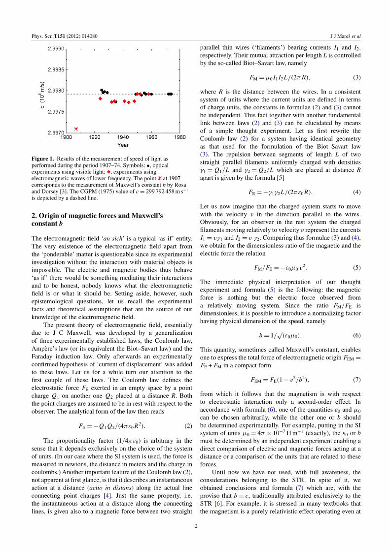
Shortly after the discovery of advanced experimentaltechniques, such as the cavity resonance method and laserinterferometry in the 1970s, enormous progress was made inincreasing the accuracy of the measurement of the speed oflight. Using a 1960 definition of meter in terms of a particularspectral line of krypton-86, and a newly constructed laserinterferometer, a group at the National Bureau of Standards,Boulder, CO (1972, [1]), obtained for the speed of light avalue c = 299 792 456.2 ± 1.1 m s−1, which was ∼100 timesless uncertain than the values accepted previously. As similarsystematic experiments conducted at that time in competinglaboratories provided results of comparable or of even betteraccuracy, the 15th Conference Generale des Poids et Mesures(CGPM) held in 1975 recommended the use of a valuec = 299 792 458 m s−1 for the speed of light. The results ofterrestrial measurements of the speed of light carried out byvarious techniques during the period 1907–74 are summarizedin figure 1. The convergence of the measured values of c to acertain constant in the last two decades is really remarkable.Due to this very fact and because of the inadequacy of thesystem of units for some metrological experiments, the 17thCGPM (1983) decided also to redefine the meter [2] in thefollowing way: ‘The meter is the length of the path traveledby light in vacuum during a time interval of 1/299 792 458 ofa second.’ The consequence of this definition is that the speedof light became an exact constant, namely

c = 299 792 458 m s−1. (1)

Apparently, such a far reaching decision was stronglyinfluenced by the general acceptance of the special theoryof relativity (STR) according to which the speed of lightis a fundamental universal constant preserving its numericalvalue in all inertial systems. It is an important property ofthis definition that it is applicable, due to the form of theLorentz transformations of time and length, not only to themeasurements of length in a rest system but also to otherinertial systems. The authors of the reform thus believed thatthe improvement of experimental techniques will not affectthe value of c, but instead it will allow us a more preciserealization of the meter.

In addition to the quite evident advantages of theintroduction of speed of light into physics and metrology inthe form of a fundamental constant having an exact value, wealso see some weak points related to such an act. A discussionof the controversial weak points summarized below is thesubject of this paper:

• the kinematic origin of the magnetic force and the natureof Maxwell’s constant b,

• Maxwell’s equations, c-equivalence principle,• transformation properties of Maxwell’s equations,

Bessel–Hagen invariants,• kinematics of light rays and the criticism of the second

postulate of the STR and• the CGPM (1983) definition of meter versus the G de

Bray scenario.

0031-8949/12/014080+07$33.00 1 © 2012 The Royal Swedish Academy of Sciences Printed in the UK

Phys. Scr. T151 (2012) 014080 J J Mares et al

Figure 1. Results of the measurement of speed of light asperformed during the period 1907–74. Symbols: •, opticalexperiments using visible light; , experiments usingelectromagnetic waves of lower frequency. The point at 1907corresponds to the measurement of Maxwell’s constant b by Rosaand Dorsey [3]. The CGPM (1975) value of c = 299 792 458 m s−1

is depicted by a dashed line.

2. Origin of magnetic forces and Maxwell’sconstant b

The electromagnetic field ‘an sich’ is a typical ‘as if’ entity.The very existence of the electromagnetic field apart fromthe ‘ponderable’ matter is questionable since its experimentalinvestigation without the interaction with material objects isimpossible. The electric and magnetic bodies thus behave‘as if’ there would be something mediating their interactionsand to be honest, nobody knows what the electromagneticfield is or what it should be. Setting aside, however, suchepistemological questions, let us recall the experimentalfacts and theoretical assumptions that are the source of ourknowledge of the electromagnetic field.

The present theory of electromagnetic field, essentiallydue to J C Maxwell, was developed by a generalizationof three experimentally established laws, the Coulomb law,Ampere’s law (or its equivalent the Biot–Savart law) and theFaraday induction law. Only afterwards an experimentallyconfirmed hypothesis of ‘current of displacement’ was addedto these laws. Let us for a while turn our attention to thefirst couple of these laws. The Coulomb law defines theelectrostatic force FE exerted in an empty space by a pointcharge Q1 on another one Q2 placed at a distance R. Boththe point charges are assumed to be in rest with respect to theobserver. The analytical form of the law then reads

FE = −Q1 Q2/(4πε0 R2). (2)

The proportionality factor (1/4πε0) is arbitrary in thesense that it depends exclusively on the choice of the systemof units. (In our case where the SI system is used, the force ismeasured in newtons, the distance in meters and the charge incoulombs.) Another important feature of the Coulomb law (2),not apparent at first glance, is that it describes an instantaneousaction at a distance (actio in distans) along the actual lineconnecting point charges [4]. Just the same property, i.e.the instantaneous action at a distance along the connectinglines, is given also to a magnetic force between two straight

parallel thin wires (‘filaments’) bearing currents I1 and I2,respectively. Their mutual attraction per length L is controlledby the so-called Biot–Savart law, namely

FM = µ0 I1 I2L/(2π R), (3)

where R is the distance between the wires. In a consistentsystem of units where the current units are defined in termsof charge units, the constants in formulae (2) and (3) cannotbe independent. This fact together with another fundamentallink between laws (2) and (3) can be elucidated by meansof a simple thought experiment. Let us first rewrite theCoulomb law (2) for a system having identical geometryas that used for the formulation of the Biot–Savart law(3). The repulsion between segments of length L of twostraight parallel filaments uniformly charged with densitiesγ1 = Q1/L and γ2 = Q2/L which are placed at distance Rapart is given by the formula [5]

FE = −γ1γ2L/(2πε0 R). (4)

Let us now imagine that the charged system starts to movewith the velocity v in the direction parallel to the wires.Obviously, for an observer in the rest system the chargedfilaments moving relatively to velocity v represent the currentsI1 = vγ1 and I2 = v γ2. Comparing thus formulae (3) and (4),we obtain for the dimensionless ratio of the magnetic and theelectric force the relation

FM/FE = −ε0µ0 v2. (5)

The immediate physical interpretation of our thoughtexperiment and formula (5) is the following: the magneticforce is nothing but the electric force observed froma relatively moving system. Since the ratio FM/FE isdimensionless, it is possible to introduce a normalizing factorhaving physical dimension of the speed, namely

b = 1/√

(ε0µ0). (6)

This quantity, sometimes called Maxwell’s constant, enablesone to express the total force of electromagnetic origin FEM =

FE + FM in a compact form

FEM = FE(1 − v2/b2), (7)

from which it follows that the magnetism is with respectto electrostatic interaction only a second-order effect. Inaccordance with formula (6), one of the quantities ε0 and µ0

can be chosen arbitrarily, while the other one or b shouldbe determined experimentally. For example, putting in the SIsystem of units µ0 = 4π × 10−7 H m−1 (exactly), the ε0 or bmust be determined by an independent experiment enabling adirect comparison of electric and magnetic forces acting at adistance or a comparison of the units that are related to theseforces.

Until now we have not used, with full awareness, theconsiderations belonging to the STR. In spite of it, weobtained conclusions and formula (7) which are, with theproviso that b ≡ c, traditionally attributed exclusively to theSTR [6]. For example, it is stressed in many textbooks thatthe magnetism is a purely relativistic effect operating even at

2

Phys. Scr. T151 (2012) 014080 J J Mares et al

negligibly small relative velocities. Argumentation in favor ofthis statement is mostly based on the fact that it is possible,by means of the kinematic principle of relativity, to derivefrom the electrostatic Coulomb law the Ampere’s law (or itsequivalent the Biot–Savart law) and the Faraday induction lawas well [7–9]. Nevertheless, as we have already seen above,the conclusion that the magnetism is a consequence of therelative motion of electric charges with respect to the observermust be more general, because it can be made without anyreference to the postulates of the STR. Moreover, in the saidrelativistic derivations based on the Coulomb law its intrinsicelement, the immediate actio in distans was tacitly used, i.e.an assumption which is absolutely at odds with the gist ofthe STR, which is conceptually a field theory postulating thefiniteness of the speed of interactions.

The effect of non-instantaneous interaction is, however,treated also in the frame of classical pre-Maxwellian theories,e.g. in [10] or especially in excellent Riemann’s posthumouspaper [11] and in a more advanced and complete form inpapers of Lienard and Wiechert [12, 13], appearing already atthe turn of the century. These authors assumed that the electricpotential or electric forces acted with a delay corresponding tothe transmission of the signal over the distance R. The actualtime of interaction is thus given by the relation

t = τ + R/b, (8)

where τ is the local time at the source of the electric force andb is the speed of electromagnetic interaction. The potentialsgenerated in this way are called retarded (Lienard–Wiechert’s)potentials. Accordingly, instead of the distance R the productKR must be inserted into formulae (2)–(4), where K is thecorrecting ‘Doppler factor’ given by [14]

K = ∂t/∂τ = 1 + (1/b) ∂ R/∂τ = 1 − (vR0) /b, (9)

where v is the velocity vector and R0 the unit vector in thedirection of the considered field point in the rest system. Letus apply this rule to the Coulomb law (2) using a somewhatspecial assumption that the vector v is parallel to the vectorR0. The Coulomb law corrected by such a special Dopplerfactor then reads

FEM = −(Q1 Q2/4πε0 R2

) (1 − v2/b2

), (10)

where the symbol FEM is used for the retarded Coulombforce. Obviously, the physical content of this formula isessentially the same as that of formula (7). Interestinglyenough, formula (10) is also identical to a central relationshipof pre-Maxwellian Wagner’s electrodynamics (written for theparticular case of zero acceleration) [10]. According to thistheory, b represents a speed limit at which the electric force isjust compensated for by the invoked magnetic force (‘. . . dieConstante b stellt dabei diejenige relative Geschwindigkeitvor, welche die elektrischen Massen Q1 und Q2 haben undbehalten mussen, wenn gar nicht mehr auf einander wirkensollen’ [10]; as we are convinced, this old idea, i.e. thatthe electromagnetic field decouple from electric charges inthe cases when its relative speed attains the value b, has anunderestimated importance).

Regardless of the fact that we have derived the‘relativistic’ formulae (7) and (10) ‘classically’ in a

very elementary way and under rather special simplifyingassumptions, it became clear that the existence of themagnetic interaction cannot be treated exclusively as arelativistic effect as is usually done. In our view, a moreadequate statement is that the STR accounts for the magnetismjust because it belongs to a wider class of theories implicitlyinvolving the concept of non-instantaneous interaction.Note in this connection that the experimentally establishedphenomenological laws (3) and (4), formulated in terms ofinstantaneous actio in distans, do not pretend to explain themagnetism but only to describe the real observations made inthe rest system. Therefore, although the algebraic operationswith formulae (3) and (4) lead to relationship (7), they are notdirectly applicable to the systems moving relatively to the restsystem.

Let us now turn our attention to the properties of theelectromagnetic field decoupled from ponderable matter.

3. Maxwell’s equations of the electromagnetic field

The structure of a hypothetical entity, an electromagneticfield in an empty space, is controlled by reduced Maxwell’sequations derived from experimentally observed lawsmentioned above. In bi-vector SI notation they can be writtenin a marvelously symmetric form due to Silberstein [15]:

rot 3 = (i/b) ∂3/∂t, (11)

div 3 = 0, (12)

where the electromagnetic complex bi-vector is defined as

3 = E + ibB, i =√

(−1). (13)

From these equations, a number of interesting conclusionscan be drawn on the basis of purely mathematical deductions.For example, it can be proved that the discontinuity in theelectromagnetic field is, in the absence of material bodies,either longitudinal stationary or constitutes a transversalvortex wave propagating with the velocity b [16]. Sincethe theory based on equations (11)–(13) describes only thefield itself (the so-called reine elektromagnetische Wellen,i.e. ‘pure electromagnetic waves’ by Silberstein) and notthe interaction with ordinary matter, the origin of suchdiscontinuities is outside the scope of the theory. It cannotbe thus, e.g., concluded that the electromagnetic wave excitedby an oscillating electric dipole spreads from the sourcewith velocity b. In many cases, the speed of energy transferrepresented by the flux of Poyinting’s vector is appreciablyslower than b [17, 18]. The transfer speed coincides with bonly in the case of ‘purely electromagnetic’ conjugate wavesfor which identically

E2= b2B2. (14)

However, condition (14) takes place practically only in theradiation zone, i.e. in the region that has sufficiently departedfrom all material bodies (sources, lenses, mirrors, etc). Itcan be stated quite generally that the speed of discontinuityof the electromagnetic field in the vicinity of ponderablematter is diminished and the speed b can be achieved only

3

Phys. Scr. T151 (2012) 014080 J J Mares et al

if the electromagnetic field is sufficiently decoupled fromthe material objects. As we believe, this effect might beresponsible for the systematically lower observed values ofthe speed of light in the cases when microwaves or millimeterwaves were used (see figure 1). The relative extent of zoneswhere condition (14) is not exactly fulfilled is appreciablylarger than that in experiments using visible light.

Nevertheless, on the basis of the substantial agreementbetween the magnitudes of c and b, Maxwell proposed (notwithout skepticism and in understandable ignorance of thefacts just mentioned!) his famous ‘Dynamical Theory ofthe Electromagnetic Field’ [19]. However, Einstein has gonemuch farther when, by postulating that in all inertial systemsthe kinematic ‘speed of the ray of the light in vacuum isconstant, being independent of movement of emitting body’(the second postulate of STR; [20]), he has implicitly assumedthat c is a universal constant identical to Maxwell’s constantb, i.e.

c = b. (15)

This relation, considered in the frame of the STR asself-evident, is now regarded to be an independent postulate,called the c-equivalence principle [21]. This principle hasnever been checked experimentally with sufficient accuracy,and therefore it bears a somewhat philosophical character.Note that the last electromagnetic measurements of Maxwell’sconstant b which were carried out in the year 1907 (asteriskin figure 1; [3]) provide a value of b differing essentiallyfrom that of c (b = 299 710 000 ± 20 000 m s−1, while theexact value of c = 299 792 458 m s−1). Later, due to thegeneral acceptance of the STR and of its second postulatethe experimentalists concentrate their efforts rather on theaccuracy of the kinematic speed of light measurements, whilethe difficult and not very exact electric measurements ofb were considered as pointless. It has to be stressed here,however, that such experiments had nothing to do withlight and that b does not primarily represent the speed oflight [22]. Restrained distinction between the electromagneticwaves and the light is felt also from Maxwell’s commentconcerning the nature of experiment for the determination ofconstants b and c [19]: ‘The value of b was determined bymeasuring the electromotive force with which the condenserof known capacity was charged, and then discharging thecondenser through a galvanometer, so as to measure thequantity of electricity in it in electromagnetic measure.The only use made of light in the experiment was to seethe instruments. The value of c found by M. Foucault wasobtained by determining the angle through which a revolvingmirror turned, while the light reflected from it went andreturned along a measured course. No use whatever was madeof electricity and magnetism.’

Maxwell’s constant b being the only parametercontrolling the behavior of a pure electromagnetic fieldin vacuum is of primary significance in all considerationsconcerning this important physical entity. We are convincedthat, as such, it cannot be identified on the basis of moreor less justified conjectures with another quantity (thespeed of light, c-equivalence principle) without a sufficientexperimental confirmation. However, recent measurementsof the constant b having comparable accuracy as that of thespeed of light are lacking. The knowledge of this constant

would thus either fill the logical gap in the present theoryor will provide a new experimental material for its furtherdevelopment.

4. Transformation properties of theelectromagnetic field

Of special interest and profound physical significance arethe transformation properties of reduced Maxwell’s equations(11)–(13) describing a pure electromagnetic field. As wasconvincingly shown by Bateman [23], reduced Maxwell’sequations are invariant with respect to the group of sphericalwave transformations, which are in fact a generalizedevocation of Huygens’ principle. Unifying in a way usual inthe STR temporal and spatial coordinates into Minkowski’sspace of four dimensions, it has been further shown thatthe spherical wave transformations can be there representedby a 15-element conformal mapping group. This group,actually identical with that studied by Sophus Lie, provides15 so-called Bessel–Hagen invariants [24]. It was shown onlylater that the number of group elements and correspondingindependent invariants could be reduced to just 11 [25].However, even after such a reduction, the number of elementsof this group exceeds the number of elements in the group ofthe Lorentz transformations as introduced in the frame of theSTR [14, 26]. The group of these transformations known frommathematics as ‘la transformation par directions reciproques’differs from that of Sophus Lie (or Bessel–Hagen), in fact,only by one element, namely by the scale transformation.The very physical meaning of this transformation can bespecified as the independence of physical processes in theelectromagnetic field from the absolute scale or dimensionsin which these processes take place or, alternatively, as theabsence of an intrinsic length in the electromagnetic field.In contrast to the pure electromagnetic field, in the worldof ponderable matter the intrinsic length scales do exist;recall e.g. the Compton length of the electron, which is λC =

2πη/mec. It is probably a fundamental fact that the existenceof intrinsic length scale in any system is conditioned by thepresence of ponderable matter [27]. Recall in this connectionMach’s conjecture claim that ‘the matter creates the space’,particularly that it defines shapes, points, etc, so that theoperative geometry cannot do without material bodies. On theother hand, any ‘as if’ entity, such as electromagnetic field,is for such a purpose quite insufficient. From this point ofview the CGPM (1983) definition of meter sounds somewhatparadoxical; the unit of length is based on the entity for whichthe concept of length is absolutely irrelevant.

Comparing now the physical content of reducedMaxwell’s equations of electromagnetic field with thatestablished within the frame of the STR, one can immediatelyrecognize that the limitations due to the introduction of thesecond postulate of the STR, from which the group of Lorentztransformations takes its origin, are quite serious. The secondpostulate eliminating the scale transformations consequentlyexcludes the existence of some important Bessel–Hageninvariants, such as the analogue of spin of the Coulombfield. This prevents us, e.g., to come to some results ofDirac’s quantum theory independently. It should also benoted that the existence of invariance of some Maxwell’s

4

Phys. Scr. T151 (2012) 014080 J J Mares et al

equations under the time-independent conformal mappingswas already discovered and used a long time ago for thesolution of electrostatic problems (cf [5]). From this pointof view the introduction of the Lorentz transformations intothe theory must be regarded as a kind of compromise usablesimultaneously for ponderable matter and electromagneticradiation, mechanics and optics [26]. Unfortunately, such acompromise leading to a strict exclusion of some potentialproperties of the electromagnetic field from theoreticalconsiderations must be classified as inconsistent.

5. Kinematic considerations

Prior to the discussion of the kinematic aspects of the speedof light, it is necessary to distinguish between the so-calledtwo-way and one-way speed of light [28]. In the two-wayspeed time-of-flight experiment, one must first trace out aclosed path for the ray of light. By clocks placed at the startingpoint, one then measures the time during which the front ofthe light ray returns back. The ratio of the length of the closedpath to the return time then defines the two-way speed oflight. The time-of-flight measurement of the one-way speedof light, and of course that of the one-way speed of anyother physical entity, requires an accurate synchronization ofthe pair of clocks placed at the initial and terminal pointsof the testing path which is topologically a line segment.However, for the realization of the synchronization procedureeither as prescribed by the STR [26, 28–31] or by using‘infinitesimally slow’ transfer of clocks [33], it is necessarya priori to assume the isotropy and the constancy of theone-way speed of light. Obviously, such a clear case ofcircular reasoning can hardly be cured by a convention givingto the one-way speed of light a certain exact value, such as(1). It would be more reasonable to admit as an experimentalfact that the measurement of one-way speeds is principallyimpossible and that the only two-way time-of-flight speedmeasurement can be realized using a closed testing path,which can do without synchronization of departed clocks.From the epistemological point of view thus the one-wayspeed of light must be excluded from our considerations andthe second postulate of the STR, in the above form, shouldbe abandoned as an empty proposition. The difficult idea ofthe light spreading from the source into all directions withthe same (one-way) constant speed c regardless of inertialsystem from which it is observed as introduced by the secondpostulate of the STR, will thus be replaced by a conceptof a light which returns along the closed path (loop) to thestarting point within the time just corresponding to the ratio =

(length of the loop/c). Of course, in such a case one can easilyimagine that the speed of light in moving inertial systems maydiffer in various points of space and directions, but only insuch a way that the time-of-flight along all isometric loopswould be the same because of some kind of ‘compensation’during the backward movement. In other words, in such aversion of the second postulate it is assumed that the two-wayspeed of light measured along different loops in differentinertial frames would represent exactly the same constant.Simultaneously, it is just the condition restricting a set ofadmissible space–time transformations reformulated in termsof two-way speed of light. Making such an assumption, it is

among others immediately clear that the Michelson–Morleyexperiment in which a split light ray is conveyed along twoisometric loops has to provide a well known ‘negative’ result,or, directly confirms the ‘two-way speed version’ of thesecond postulate.

Basing on these ideas, it starts to be apparent thatthe most problematic operation in measuring speeds is thesynchronization of clocks at departed stations. Therefore, letus mention here the standard technique for the determinationof one-way delay time tA necessary for propagation oflight signal from point ‘1’ to another point ‘2’ whichseemingly circumvents the synchronization of the clocks [32].(This technique was also used, e.g. in famous OPERAexperiment [34] where superluminous speed of neutrino wasreputedly indicated.) Split light signal is sent from point ‘1’via two alternative paths A (direct) and B (slightly longer)to point ‘2’, where the time difference tA − tB is measuredbetween arrivals of both signals. After that the total timetA + tB is measured, which is necessary for the propagation ofthe signal from ‘1’ to ‘2’ along the path A and back to point‘1’ along the path B. The time tA, which we are interested in,can be then computed by an obvious formula

tA =12 [(tA + tB) + (tA − tB)]. (16)

Evidently, the method is fully based on the assumption thatthe time tB needed for the signal propagation along the pathB from ‘1’ to ‘2’ is exactly the same as that for backwardpropagation from ‘2’ to ‘1’. Such an assumption is, however,equivalent to the validity of the second postulate of STR,a statement for which the experimental evidence is in factlacking. Admitting instead of the two-way speed versionof the second postulate confirmed by the experiments, thetimes corresponding to the signal propagation in oppositedirections may generally differ, i.e. tB(1 → 2) 6= tB(2 → 1),which makes formula (16) useless. In such a case theresults of speed measurements based on it will be inevitablyspurious. This example clearly illustrates that the secondpostulate of STR is not only redundant but that it can be alsoharmful.

The redundancy and arbitrariness of the second postulateof the STR was recognized by a group of Chinese researcherswho formulated a theory of relativity which can do withoutsecond postulate intimately related to the speed of light [35].This is so-called ‘Taiji relativity’. (The term ‘Taiji’ is a centralconcept of ancient Chinese cosmology having a meaning ofultimate principle existing before the creation of the Universe.As such, it is akin to the European term apeiron—απειρoν.)It claims among others that the relativity of time and theuniversality of speed of light are not physical entities inherentin nature but human conventions imposed upon it. The Taijitheory is in fact essentially based on the experimentallyconfirmed two-way speed version of the second postulate ofthe STR as formulated above, according to which the two-wayspeed must be isotropic in all inertial frames.

The fact that only the two-way speed of light has physicalmeaning has its consequences also for the realization of themeter according to its CGPM (1983) definition. The authorsof this definition and recommendations for the practicalrealization of the meter normal (mise en pratique [2]), namely,tacitly count with the possibility of one-way measurement of

5

Phys. Scr. T151 (2012) 014080 J J Mares et al

the speed of light and with their full awareness admit thepostulates of the STR. The shape of the test path need notbe thus specified and the time measurement, particularly thesynchronization of clocks, is done according to the ‘acceptedgood practice’ which follows the rules of STR. Astonishingly,it is further assumed that the measurements are restricted tothe lengths which are sufficiently short to be negligible forthe effects belonging to the scope of general relativity (e.g.gravitation). Such an assumption logically challenges the factthat the universal constant c is ‘universal’ and ‘constant’. It isthus apparent that the critical reconsideration of the definitionand of allied problems is necessary.

Taking into account the fact that the most accuratearrangements for the optical measurements of the speedof light operate as a two-way laser interferometers ofFabry–Perot type where the test path is enclosed betweentwo parallel semi-permeable mirrors, the normal of lengthcan be quite naturally realized just by the distance betweenthese two plains. However, the distance defined in this waycan be converted into terms inherent to the CGPM (1983)definition only by a consequent use of the second postulate ofSTR. The CGPM (1983) definition thus makes this postulateconceptually indispensable although it has for the practicalrealization of the normal of length no significance.

6. G de Bray scenario

As was already mentioned above, according to the CGPM(1983) definition of meter and to the corresponding miseen pratique, the measurements should be restricted to thelengths which are ‘sufficiently’ short in order not to beinfluenced by gravitation etc. Beside the space-related effects,however, there can possibly also be the time drift of thevalue of c. To this effect turned attention G de Bray whoafter the careful revision of experiments made by variousresearchers between the years 1849–1933 concluded that theearlier observations give a higher speed of light [36]. Such abehavior of the ‘pseudoconstant’ c has been attributed by theauthor to the apparent decrease of the unit of length caused bythe expansion of the Universe. If the radius of the Universedoubles every K years, then the measured velocity of lightwill be halved every K years, that is, the velocity will beproportional to c ∝ (1/2)τ/K , where τ is here time in years.Of course, an enormous increase of accuracy of measurementsand the constancy of the speed of light during the secondhalf of the 20th century made the G de Bray scenario highlyimprobable. Nevertheless, to be correct, the long-term driftof c can be hardly excluded or proved on the basis of sayaround ten measurements made during two decades only(see figure 1). Since the influence of cosmological effectsbelonging to the scope of general relativity cannot be apriori excluded even for terrestrial observations, the CGPM(1983) definition anticipating in fact the absolute impossibilityof G de Bray scenario sounds rather bold and not verywise. Moreover, as we have seen above, the CGPM (1983)definition is not a plain technicality but it contains hiddenassumptions which can make the analysis of experimentsconfused and difficult.

7. Conclusions

In the present contribution we have discussed, as we believe,a legitimate question, what the consequences of the CGPM(1983) definition of meter are, especially of the fixation ofthe speed of light at the exact value c = 299 792 458 m s−1.This question has important aspects which, remaining in theshade of the STR, are discussed in the current literature onlymarginally. However, as we are convinced, their omission maylead and led to the incorrect conclusions or to the maskingof real effects. Therefore, these aspects should be analyzedcritically and repeatedly. Some of them were discussed in thispaper with the following conclusions.

First of all, we have summarized the arguments in favorof the idea that the magnetic force is a manifestation of theelectric force in relative movement. We have shown that sucha picture is independent of STR and of its second postulateand that the square of Maxwell’s constant b controlling theratio of the electric and the magnetic force in any particularsituation is not necessarily related to the speed of light, c.

Although we are not convinced that the c-equivalenceprinciple is not valid (c 6= b), we have stressed that itsexperimental confirmation is at present lacking. Conse-quently, there is a serious logical gap in the electro-magnetic theory of light and all related theories as well.According to our meaning, it is thus quite necessary to repeatthe measurements of b with an accuracy comparable with thatof the speed of light in the near future.

Considering the description of the electromagnetic field,we have turned our attention to the fact that the transformationgroup of Maxwell’s equations is larger than the Lorentzgroup, in other words that there are invariants (Bessel–Hageninvariants) and properties of the electromagnetic field that areoutside the scope of the STR. This fact may have a number ofimportant consequences which should not be omitted only onthe basis of a teleological argument, i.e. because they do notfit well the STR.

In the paragraph concerning the kinematic problems wehave pointed out the principal impossibility of measuring theone-way speed of light and other physical entities. Therefore,we have suggested a ‘two-way speed’ version of the secondpostulate of the STR which fits well the known experimentalobservations and in some cases effectively eliminates thedifficulties with synchronization of clocks. Some featuresof this approach are shared by the so-called Taiji theory ofrelativity which left out the second postulate of the STRcompletely. As we have further shown, ignorance of theprincipal impossibility of measuring the one-way speeds maylead to serious experimental errors and misinterpretations.

The CGPM (1983) definition anticipates the absoluteimpossibility of the scenario of G de Bray’s type, i.e. ofa slow drift of the speed of light, although such a drift iscompatible with the predictions of, e.g., the general theory ofrelativity. We are therefore convinced that the measurementsof the speed of light should remain the subject of astrophysicalexperimental research in future, in spite of the fact that theyalready lost their formal sense.

Last but not least, although we criticized, in this paper,among others, one of the cornerstones of modern physics, thesecond postulate of the STR, our aim was by no means to

6

Phys. Scr. T151 (2012) 014080 J J Mares et al

belittle the merits and great efforts of scientists such as WVoigt, J Larmor, H A Lorentz, H Poincare and A Einsteinwho established the STR more than 100 years ago but onlyto direct attention to the problems which should be solved.Let us therefore add a quotation from the paper of one ofthe creators of the STR (Poincare [32]) which elucidates ourattitude: ‘Good theories are flexible. . . . Specious argumentshave no effect on them, and they also triumph over all seriousobjections. However, in triumphing they may be transformed.’

References

[1] Bureau International des Poids et Mesures 1983Resolution 1 of the 17th meeting of the CGPMwww.bipm.org/en/CGPM/db/17/1/

[2] Quinn T J 2003 Practical realization of the definitionof the metre, including recommended radiationsof other optical frequency standards (2001) Metrologia40 103–33

[3] Rosa E B and Dorsey N E 1907 A new determination of theratio of the electromagnetic to the electrostatic unit ofelectricity Bull. Bur. Stand. 3 433–604

[4] Maxwell J C 1875 On action at a distance Proc. R. Inst. GB7 44–54

[5] Smythe W R 1968 Static and Dynamic Electricity 3rd edn(New York: McGraw-Hill)

[6] Rosser W G V 1968 Classical Electromagnetism via Relativity(London: Butterworths)

[7] Page L 1912 Eine Ableitung der Grundbeziehungen derElektrodynamik aus jenen der Elektrostatik Phys. Z.13 609–15

[8] Matveev A N 1980 Elektrodinamika 2nd edn (Moscow:Vysshaya Shkola)

[9] Frisch D H and Wilets L 1956 Development of theMaxwell–Lorentz equations from special theory of relativityand Gauss’s law Am. J. Phys. 24 574–9

[10] Weber W and Kohlrausch R 1856 Ueber die Elektrizitatmengewelche bei galvanischen Stromen durch den Querschnitt derKette fliesst Ann. Phys. 175 10–25

[11] Riemann B 1867 Ein Beitrag zur Elektrodynamik Ann. Phys.207 237–43

[12] Lienard A 1898 Champ electrique et magnetique L’EclairageElectr. 16 5–14

Lienard A 1898 L’Eclairage Electr. 16 53–9Lienard A 1898 L’Eclairage Electr. 16 106–12

[13] Wiechert E 1901 Elektromagnetische Elementargesetze Ann.Phys. 309 667–89

[14] Schott G A 1912 Electromagnetic Radiation and theMechanical Reactions Arising from It (Cambridge:Cambridge University Press)

[15] Silberstein L 1907 Elektromagnetische Grundgleichungen inbivektorieller Behandlung Ann. Phys. 327 579–86

[16] Silberstein L 1908 Uber elektromagnetischeUnstetigkeitsflachen und deren Fortpflanzung Ann. Phys.331 751–62

[17] Bateman H 1915 The Mathematical Analysis of Electrical andOptical Wave—Motion on the Basis of Maxwell’s Equations(Cambridge: Cambridge University Press) (reprints: Dover,1955, Russian translation: GIFML, Moscow, 1958)

[18] Jackson J D 1999 Classical Electrodynamics 3rd edn(New York: Wiley)

[19] Maxwell J C 1865 A dynamical theory of the electromagneticfield Phil. Trans. R. Soc. 155 459–512

[20] Einstein A 1910 Principe de relativite et ses consequences dansla physique moderne Arch. Sci. Phys. Nat. Ser. 4 29 5–28

Einstein A 1910 Arch. Sci. Phys. Nat. Ser. 4 29 125–44[21] Heras J A 2010 The c-equivalence principle and the correct

form of writing Maxwell’s equations Eur. J. Phys.31 1177–85

[22] Maxwell J C and Jenkin F 1863 On the elementary relationsbetween electrical measurements British Association ofAdvancement of Science Report appendix C 130–54

[23] Bateman H 1910 The transformation of the electrodynamicalequations Proc. Lond. Math. Soc. 8 223–64

[24] Bessel-Hagen E 1921 Uber die Erhaltungssatze derElektrodynamik Math. Ann. 84 258–76

[25] Plybon B F 1974 Observations on the Bessel–Hagenconservation laws for electromagnetic fields. Am. J. Phys.42 998–1001

[26] Einstein A 1905 Zur Elektrodynamik der bewegter KorperAnn. Phys. 17 891–921

[27] Ivanenko D and Sokolov A 1949 Klassitsheskaya TeoriyaPolya (Leningrad: GITL)

[28] Perez I 2011 On the experimental determination of theone-way speed of light Eur. J. Phys. 32 993–1005

[29] Voigt W 1887 Uber das Doppler’sche Princip Goett. Nachr.2 41–51

[30] Larmor J 1897 A dynamical theory of the electric andluminiferous medium Phil. Trans. R. Soc. A 190 205–300

[31] Lorentz H A 1892 La Theorie electromagnetique de Maxwellet son applicationaux corps mouvants Arch. NeerlandaisesSci. Exactes Nat. 25 363–552

[32] Poincare H 1900 La theorie de Lorentz et le principe dereaction Arch. Neerlandaises Sci. Exactes Nat. 5 252–78

[33] Votruba V 1969 Zaklady specialnı teorie relativity (Academia:Praha)

[34] Adam T et al 2012 Measurement of the neutrino velocity withthe OPERA detector in the CNGS beam J. High EnergyPhys. JHEP10(2012)093 (arXiv:1109.4897v4)

[35] Hsu J P and Hsu L 1994 A physical theory based solely on thefirst postulate of relativity Phys. Lett. A 196 1–6

[36] Gheury de Bray M E J 1936 The velocity of light Isis25 437–48

7

2. PHENOMENOLOGICAL MEANING OF TEMPERATURE

Jiří J. Mareš

Dolus latet in universalibus 2.1. Introduction

It is difficult to imagine the immense effort which was necessary for the

transformation of ancient theory of thermal phenomena based on the peripatetic concepts of Antiperistasis and Doctrine of Four Elements (coldness, hotness, dryness, humidity) [1,2] into the modern system based on measurable quantities having definite magnitudes and physical dimensions, which would be convenient for effective mathematical processing. Path-breaking statement “Coldness is nothing but the absence of hotness” which can be found in the Galileo’s correspondence with his pupils [3] and denying the very fundaments of Aristotelian physics, was probably even more heretical than his famous statement concerning the rotation of Earth. It should be noticed here that the research into the thermal phenomena is enormously difficult in comparison with e.g. the research into the mechanics because the concepts involved are of very abstract nature. For example, it took an appreciable time, more than ~150 years, till the “intensive” and “extensive” aspects of heat were in a pregnant way introduced into the thermal physics by J. Black [4], where they substituted a vague term of “heat” closely related to our sensations. Another serious obstacle in the development of thermal physics is its universality. Considering namely any process in the nature, one immediately recognizes that it is controlled or at least influenced by the “thermal” conditions in which it takes place. Therefore the theory of thermal phenomena has to be inevitably quite universal and consequently very prone to misinterpretations and far reaching persistent errors (according to our motto in the heading, “Deception is concealed in the universality”). Keeping thus in mind just this last important circumstance, we have made an attempt to outline anew the logical structure of the phenomenological thermal physics which is, as we are convinced, far from being well established. In this short review we have focused our attention mainly on one crucial concept of the thermal physics, namely on the temperature.

What does the temperature actually mean? It is a classically simple question astonishingly lacking an appropriate answer. The answers, namely, which can be found in the textbooks on thermodynamics, are only hardly acceptable without serious objections. For illustration, let us give a few typical examples here and the reader himself can easily find others in the current literature. To the most hand-waving belong the statements such as that “the temperature is known from the basic courses of physics” or even “temperature is known intuitively”. More frankly sounds the practical formulation that “the temperature is reading on the scale of thermometer” throwing doubt, perhaps without awareness, upon the very existence of temperature if the thermometer is not at our disposal. In contrast to it, rather philosophical is the statement that “temperature is a physical property of a system that underlies the common notions of hot and cold” which, nevertheless, rather specifies what the temperature should be, giving no idea of what it actually is. To a high scientific standard pretends the definition telling us that “on the macroscopic scale the temperature is the unique physical property that determines the direction of heat flow between two objects placed in thermal contact” being in fact an explanation obscurum per obscurius which transforms the temperature problem to the problem of flow of something even more uncertain. In order not to

fall, however, into an unfertile and non-constructive criticism we stop now with examples the purpose of which was only to illustrate the state of affairs and turn our attention to the other aspects of the problem.

Of course, there is no doubt that the temperature is a central concept of thermal physics and therefore a lot of researchers feeling the lack of a good definition were trying, in different ways, to bring the temperature concept on the safer grounds. For example, the authors preferring the axiomatic approach are, as a rule, inclined to assume that the temperature is a primitive concept which need not be, in principle, derived from other presumable more primitive ideas. Unfortunately, the experimental determination of temperature in any particular case requires performing a lot of non-trivial operations which should be substantiated by its definition. Thus such a shift from the operative physical definition to the metaphysical one, very comfortable for theoreticians, makes an inexplicable obscure ritual any actual temperature measurement performed by experimentalists.

For researchers who consider the thermal physics being nothing but an outgrowth of statistical mechanics, the equilibrium temperature of a system can be (up to an arbitrary factor) defined as an inverse of the derivative of natural logarithm of the statistical weight of its actual macroscopic state with respect to the energy of the system. Nevertheless, practically no actual measurement of temperature is directly linked with the evaluation of statistical data related to a certain ensemble of particles and excitations but it is as a rule performed by means of various forms of thermometers converting the temperature to another measurable physical quantity. It is thus evident that prior to the identification of the temperature defined in the frame of statistical theory with the phenomenological temperature, the latter has to be satisfactorily defined first.

The purpose of this contribution is thus to re-examine a fundamental concept of thermal physics, temperature, partly from the historical and partly from a logical point of view. In order to avoid very general abstract considerations the exposition is confined practically only to fluids, i.e. mechanical systems for which are the constitutive relations simple and well known. The mathematical structure of the precursor of temperature, hotness manifold, is, as far as we know, for the first time discussed in terms of elementary set theory. In the exposition of the subject the emphasis is put on experiment and on the generalization of empiric data while mathematical proofs of some statements has reader confer with special references already given.

2.2. Phenomenological conjugate variables

The very task of any mathematical theory of material systems is to establish general

rules for the further treatment of empirical constitutive relations describing the state of a body in terms of suitably chosen parameters. We do not mean here the parameters specific for the description of thermal effects but just the parameters already introduced in other branches of physics and generally known as the phenomenological variables [5]. The existence of such variables, playing the roles of macroscopic conditions which are compatible with a huge number of parameters describing each microscopic component of the body, is clearly a matter of experience. Usually, there is an appreciable number of various phenomenological variables determining the state of the body but fixing a chosen one by external means, this number can ever be diminished by one. Continuing such a procedure the number of significant phenomenological variables can be finally reduced to two. It is a fact worth to noticing that the two-parameter system is the simplest model of a real system because it enables one to construct a meaningful constitutive relation and, simultaneously, it is apt for straightforward generalization, e.g. by adding another pair of independent variables. In order to ensure easy perceptibility of mathematical description of two-parameter systems a special form of

phenomenological variables was found to be desirable. It is a well known fact that the terms entering the energy balance equations in mechanics and electrodynamics have a canonical form which may be characterized by means of the following dimensional relation

[Energy] = [X] × [Y ], (1)

where square brackets mean the physical dimension of the quantities enclosed. As the energy is an extensive quantity, it is favourable for first phenomenological variable to choose also an extensive quantity, say X. In such a case, however, the second parameter has to be inevitably an intensive quantity, Y [6]. Such a couple of quantities obeying relation (1) is then called a couple of conjugate variables. (For example, the list of the most frequently used conjugate parameters is given in Table 1.) The existence of the intensive and extensive “aspects” of heat which was already recognized by J. Black [4] is thus in this context the discovery of primary importance for the formalization of theory of heat and its compatibility with other branches of physics. His “intensity of heat” and “matter of heat” can be, namely, quite naturally assigned to a certain couple of conjugate variables, which may be tentatively called „temperature „ and „heat“. Formal compatibility of these two quantities with the system of quantities already introduced in other branches of physics is thus only a matter of proper choice of suitable operative definitions and units.

Table 1. Selected conjugate variables

Extensive Intensive Energy quantity X quantity Y term E

Volume V pressure p pV Momentum G velocity v vG Charge Q el. potential φ φQ Mass M grav. pot. γ γM

2.3. Diathermic partition, thermal equilibrium

The idea to treat real system in terms of conjugate variables enable one to introduce

some fundamental concepts of thermal physics in a quite systematic way and, somewhat astonishingly, without a priori reference to the thermal phenomena per se, particularly to the quantities of temperature and heat [7]. The important role plays here the so called correlation test. It is the procedure frequently used in the practical thermometry which enables one to check whether the thermometer is in proper thermal contact with the measured body. Simultaneously, it provides the basis for the following operational definition of diathermic and adiabatic partitions (walls), viz: Let us have two systems characterized by couples of conjugate variables (X,Y) and (X‘,Y‘), respectively, and separated by a macroscopically firm material partition (wall) defining their common boundary. Such a partition is called diathermic if the changes of the variables (X,Y) induce the changes of the variables (X‘, Y‘) and vice versa (“diathermic“ originates from Greek διά = through, θερμóς = warm). A concept complementary to that of diathermic partition is the adiabatic partition (from Greek α- = negation, διά = through, βαίνειν = to go) which prevents the thermal contact of neighbouring bodies, i.e. ensures their thermal insulation. Obviously this concept is a limiting one, depending to an appreciable extent on the accuracy of the correlation test. The adiabatic

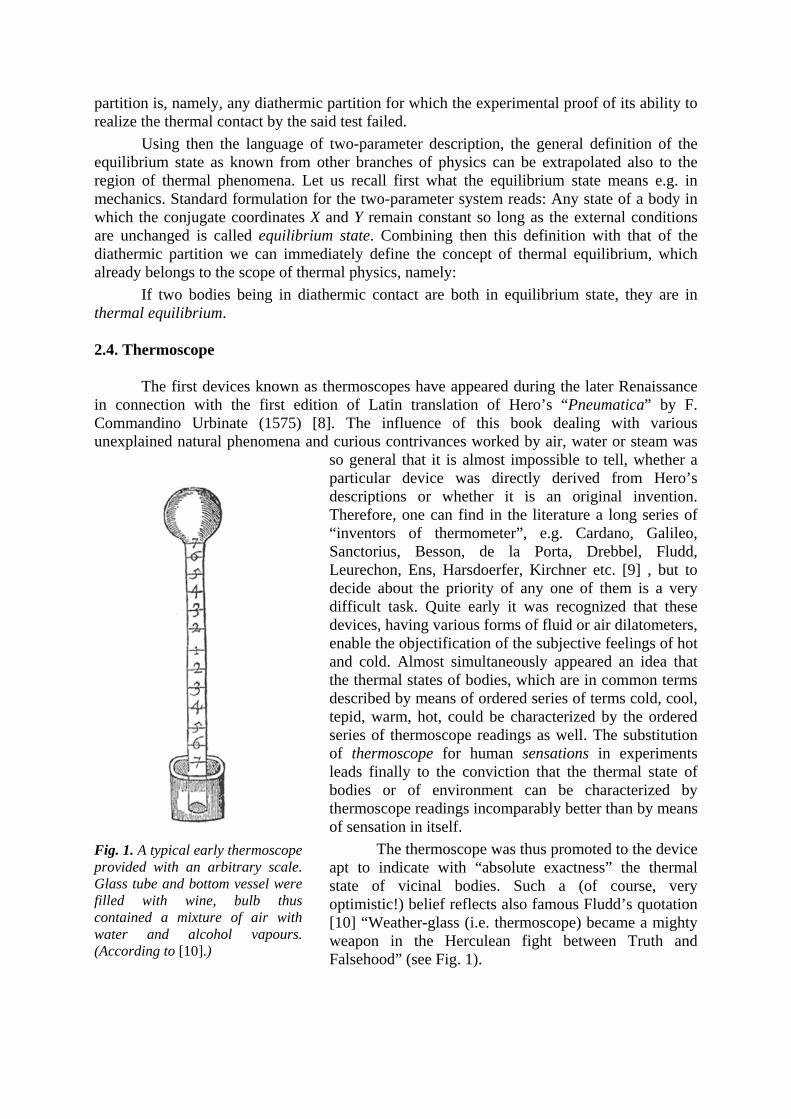
partition is, namely, any diathermic partition for which the experimental proof of its ability to realize the thermal contact by the said test failed.

Using then the language of two-parameter description, the general definition of the equilibrium state as known from other branches of physics can be extrapolated also to the region of thermal phenomena. Let us recall first what the equilibrium state means e.g. in mechanics. Standard formulation for the two-parameter system reads: Any state of a body in which the conjugate coordinates X and Y remain constant so long as the external conditions are unchanged is called equilibrium state. Combining then this definition with that of the diathermic partition we can immediately define the concept of thermal equilibrium, which already belongs to the scope of thermal physics, namely:

If two bodies being in diathermic contact are both in equilibrium state, they are in thermal equilibrium. 2.4. Thermoscope

The first devices known as thermoscopes have appeared during the later Renaissance in connection with the first edition of Latin translation of Hero’s “Pneumatica” by F. Commandino Urbinate (1575) [8]. The influence of this book dealing with various unexplained natural phenomena and curious contrivances worked by air, water or steam was

so general that it is almost impossible to tell, whether a particular device was directly derived from Hero’s descriptions or whether it is an original invention. Therefore, one can find in the literature a long series of “inventors of thermometer”, e.g. Cardano, Galileo, Sanctorius, Besson, de la Porta, Drebbel, Fludd, Leurechon, Ens, Harsdoerfer, Kirchner etc. [9] , but to decide about the priority of any one of them is a very difficult task. Quite early it was recognized that these devices, having various forms of fluid or air dilatometers, enable the objectification of the subjective feelings of hot and cold. Almost simultaneously appeared an idea that the thermal states of bodies, which are in common terms described by means of ordered series of terms cold, cool, tepid, warm, hot, could be characterized by the ordered series of thermoscope readings as well. The substitution of thermoscope for human sensations in experiments leads finally to the conviction that the thermal state of bodies or of environment can be characterized by thermoscope readings incomparably better than by means of sensation in itself.

Fig. 1. A typical early thermoscope provided with an arbitrary scale. Glass tube and bottom vessel were filled with wine, bulb thus contained a mixture of air with water and alcohol vapours. (According to [10].)

The thermoscope was thus promoted to the device apt to indicate with “absolute exactness” the thermal state of vicinal bodies. Such a (of course, very optimistic!) belief reflects also famous Fludd’s quotation [10] “Weather-glass (i.e. thermoscope) became a mighty weapon in the Herculean fight between Truth and Falsehood” (see Fig. 1).

2.5. Thermoscopic states In order to continue this story in a more contemporary and systematic way we will call

thermoscope any two-parameter system in which one of the conjugate parameters, say Y, can be fixed, Y = Y0. It is further assumed that thermoscope can be brought into a diathermic contact with other bodies and that it is sufficiently “small” in comparison with these bodies in order to not appreciably disturb their thermal equilibrium. The second conjugate real parameter X, which is called in this connection thermoscopic variable, is generally of quite a diverse physical nature and dimension. It may be length, volume, resistance, voltage, frequency and many others. In order to distinguish formally among various thermoscopic variables, differently constructed thermoscopes and physical conditions under which they operate, a small Latin index is used. Applying this convention, reading Xk(P) of the k-th thermoscope which is in diathermic contact with a body under investigation defines the thermoscopic state P of the body. The corresponding set of the thermoscopic states which can be observed in this way is then marked as Hk. Notice that the readings Xk are related to the thermoscope while the indicated thermoscopic state as e.g. P ∈ Hk, already relates to the body. It is a matter of fact that the phenomenological parameters were introduced into classical mechanics and electrodynamics as continuous quantities covering certain closed intervals of real axis. Therefore, according to our definitions, such a property is transferred also to the thermoscopic variables Xk. We will thus assume that the numerical values of quantity Xk also continuously cover a certain closed interval Ik, operation range of the k-th thermoscope, which is a proper part of the set of real numbers, E1. In usual symbols we can thus write1: Xk ∈ Ik ⊂ E1. (2) If it is further for every couple P, Q ∈ Hk,

P ≠ Q , ⇔ Xk(P) ≠ Xk(Q), (3)

the set Hk can be ordered in accordance with the intrinsic order already existing in real interval Ik ⊂ E1. Simultaneously, condition (3) ensures the existence of one-to-one mapping between the sets Ik and Hk and we can thus define order ( p, f) in Hk by the following equivalences: P p Q ⇔ Xk(P) < Xk(Q) P f Q ⇔ Xk(P) > Xk(Q) (4a-c) P = Q ⇔ Xk(P) = Xk(Q) Moreover, we have a liberty of choosing the “arrow” indicating the order because the symbols <, > on the right side of relations (4a,b) can be changed, according to our need, into >, <.

It is apparent that conditions (4a-c) provide basis for the construction of a primitive temperature scale. Indeed, unambiguous assignment of a certain value Xk(P) to every state P ∈ Hk is nothing but realisation of a local empirical temperature scale in terms of thermoscopic variable Xk. It is, however, an important fact belonging rather to the scope of epistemology, that although the empirical scales enable one to characterize the thermal states

1 We do not distinguish here the physical quantity and its corresponding numerical value. See also [6].

of bodies, for the revealing of the very nature of physical quantity called temperature are almost useless and further development of more involved concepts is thus necessary.

There is another requirement ensuring the objectivity of the above conception. It is so called Principle of indifference according to which different thermoscopes k, j operating in the common range of thermoscopic states should distinguish any two different states P ≠ Q,

P, Q∈(Hk∩Hj), regardless of their construction, thermometric substances, variables X and other physical conditions used. A procedure worked out by Dulong and Petit [11] is used in practical thermometry for the comparison of different empirical temperature scales. So called Dulong-Petit plot is a locus of readings Xk of one thermoscope versus readings Xj of another thermoscope both being in thermal contact with the same body (thermal bath). Evidently, in terms of such a plot the Principle of indifference may be formulated simply as follows: Two empirical temperature scales agree with the Principle of indifference just if their Dulong-Petit plot is

monotonic. Interestingly, very similar method was used much earlier by savants of Accademia del Cimento who discovered in this way, just above the freezing point of water its anomaly (i.e. non-monotonic Dulong-Petit plot with respect to the other at that time known thermoscopes, see Fig. 2) [12], which excludes the water from being in this range a suitable thermometric substance.

Fig. 2. Dulong-Petit plot of an alcohol-filled thermometer (Gradus thermometris) vs. readings on dilatometer (Gradus vasis) filled with fresh water showing the so called water anomaly. Data were obtained by Accademia del Cimento about 1660. [2,12]

2.6. The use of fixed points for calibration of thermoscopes

An appreciable irreproducibility of early thermoscopes was a serious obstacle for development of non-peripatetic thermal physics. There were attempts to improve the situation by making exact copies of a standard instrument and by sending them to the various laboratories where they were intended to serve as secondary standards [12]. This, theoretically correct approach had nevertheless lot of practical limitations. It required a really high reproducibility of glass-blowing and preparation of glass and thermometric substances. Consequently, standard “thermometers” were very expensive and the transport of such delicate instruments over the long distances was quite risky. Therefore an important qualitative step toward the scientific thermometry was done when the so called fixed thermometric points were discovered and became in general use. The fixed point is called a body prepared by a definite prescription revealing by some observable qualitative property its physical state (e.g. boiling point of helium, melting point of water, melting point of platinum – all at normal atmospheric pressure) and which being in thermal equilibrium with other bodies defines unambiguously their thermoscopic state. Fixed points thus may serve as a mean for realization of fiducial points on empirical temperature scales corresponding to the

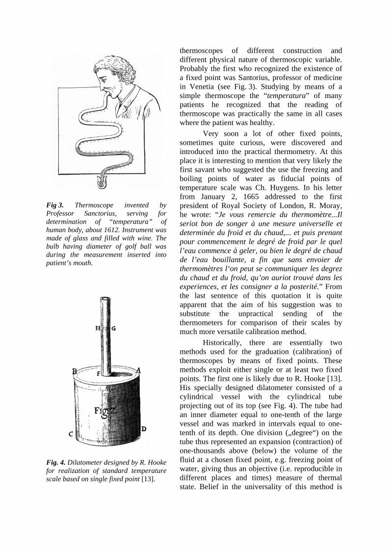
thermoscopes of different construction and different physical nature of thermoscopic variable. Probably the first who recognized the existence of a fixed point was Santorius, professor of medicine in Venetia (see Fig. 3). Studying by means of a simple thermoscope the “temperatura” of many patients he recognized that the reading of thermoscope was practically the same in all cases where the patient was healthy.

Fig 3. Thermoscope invented by Professor Sanctorius, serving for determination of “temperatura” of human body, about 1612. Instrument was made of glass and filled with wine. The bulb having diameter of golf ball was during the measurement inserted into patient’s mouth.

Fig. 4. Dilatometer designed by R. Hooke for realization of standard temperature scale based on single fixed point [13].

Very soon a lot of other fixed points, sometimes quite curious, were discovered and introduced into the practical thermometry. At this place it is interesting to mention that very likely the first savant who suggested the use the freezing and boiling points of water as fiducial points of temperature scale was Ch. Huygens. In his letter from January 2, 1665 addressed to the first president of Royal Society of London, R. Moray, he wrote: “Je vous remercie du thermomètre...Il seriot bon de songer à une mesure universelle et determinée du froid et du chaud,... et puis prenant pour commencement le degré de froid par le quel l’eau commence à geler, ou bien le degré de chaud de l’eau bouillante, a fin que sans envoier de thermomètres l‘on peut se communiquer les degrez du chaud et du froid, qu’on auriot trouvé dans les experiences, et les consigner a la posterité.” From the last sentence of this quotation it is quite apparent that the aim of his suggestion was to substitute the unpractical sending of the thermometers for comparison of their scales by much more versatile calibration method.

Historically, there are essentially two methods used for the graduation (calibration) of thermoscopes by means of fixed points. These methods exploit either single or at least two fixed points. The first one is likely due to R. Hooke [13]. His specially designed dilatometer consisted of a cylindrical vessel with the cylindrical tube projecting out of its top (see Fig. 4). The tube had an inner diameter equal to one-tenth of the large vessel and was marked in intervals equal to one-tenth of its depth. One division („degree“) on the tube thus represented an expansion (contraction) of one-thousands above (below) the volume of the fluid at a chosen fixed point, e.g. freezing point of water, giving thus an objective (i.e. reproducible in different places and times) measure of thermal state. Belief in the universality of this method is

based on a tacit assumption that a dilatometer and thermometric substance used can reveal all in the nature accessible thermal states.

The first significant attempt at application of two-point calibration of thermometers belongs to members of Accademia del Cimento (1657-1667) [14]. They divided into three hundred degrees the interval between two marks indicating somewhat vague “fixed points”, namely, the greatest summer heat and the most severe winter cold. Two-point calibration

technique but based on more reliable fixed points, melting point of ice and boiling point of water (incidentally the fiducial points which were proposed much earlier by Huygens!) were used also by C. Rinaldini (1693) for realization a his 12-degree thermometric scale. This well-done temperature scale was never in general use, however, a half century later, in hands of Celsius [15], became essentially the same scale the basis of our centigrade thermometric system. On the problem of graduation of thermometers worked independently Danish astronomer O. Rømer, and especially his immediate follower, German instrument maker G. D. Fahrenheit, who had used large deal of Rømer’s know-how [16]. Accordingly, Fahrenheit accepted as a lower fixed point mixture of salt and ice (0°F) and normal body temperature (96°F) as the upper one. The freezing point of water (32°F) was retained as a subsidiary calibration point [17]. Enormous care was devoted to the purification of thermometric substance, mercury, improvements of glass-blowing procedure and exact specification of conditions for realization of fixed points. As a result, Fahrenheit’s thermometers were much admired throughout the scientific community for their accuracy and extraordinary reproducibility and became thus for a long time a thermometric standard. In 1742 Swedish astronomer A. Celsius created a two-fixed point’s temperature scale whereby zero represented the boiling point of water and one hundred represented the freezing point of water (see Fig. 5). In his lectures announced the observations showing that melting point of ice was effectively unaffected by pressure. He also determined with remarkable precision how boiling point of water varied as a function of atmospheric pressure and proposed that zero on his temperature scale (= boiling point of water) would be calibrated at the mean barometric pressure at mean sea level (standard

atmosphere). As his scale was intended for meteorological observations where the temperatures are always below the temperature of boiling point of water, the scale was, in order to avoid the changes of the sign, reverted in comparison with the contemporary centigrade scale. Two years later, however, the famous Swedish botanist C. Linnaeus changed the Celsius’s scale in order to be more convenient for the use in his greenhouse, constructing the thermometric scale where zero represented the melting point of ice and 100 represented boiling point of water. As the “centigrade” system was compatible with the philosophy of

Fig. 5. An example of graduation of a thermometer by means of two-fixed point’s method. Figure depicts a thermometer provided with the original “reverted” centigrade scale (Celsius, 1742). It is also shown the uncertainty of boiling point of water (=zero) which is due to fluctuations of barometric pressure [15].

metric centesimal system the Celsius’s scale became later to the scale almost exclusively used on the Continent [15].

2.7. Mach’s postulates

Importance of fixed points for thermometry is, however, not confined only to the

calibration of thermoscopes but as was recognized not before the end of 19th century their theoretical significance is much more general. Quite interestingly, it has been originally taken for a self-evident empirical fact that it is always possible to find in an operation range of any thermoscope a sufficient number of fixed points enabling calibration of a local empirical scale, sewing it up with other overlapping empirical scales and to check, by means of the Dulong-Petit plots, the validity of Principle of indifference. The choice of fixed points for such purposes was quite pragmatic, respecting especially their easy realization, suitable distribution and stability (see e.g. Table 2). The very fact that such a liberty of choice can only be a consequence of the existence of enormous (if not infinite) number of fixed points falling into any interval of thermoscopic states remained for a long time quite unnoticed. Similar fate, i.e., being effectively undiscovered, has also the fact that the fixed points can be always found out of any interval of thermoscopic states.

Table 2. Selection of fixed points of the ITS-90

Substance State T90/K

Cd S 0.5190 Zn S 0.8510 Al S 1.1796 In S 3.4145 Pb S 7.1996 e-H T 13.8033 Ne T 24.5561 O2 T 54.3584 Ar T 83.8058 Hg T 234.3156 H2O T 273.1600 Ga M 302.9146 In F 429.7485 Sn F 505.0780 Zn F 692.6770 Al F 933.4730 Ag F 1234.9300 Au F 1337.3300 Cu F 1357.7700

S – superconductivity transition T – triple point M – melting point F – freezing point (both at a pressure of 101325 Pa)

These and other experimentally observed properties of fixed points have been generalized by means of method of incomplete induction, the reasoning according to which the conclusion related even to the infinite number of cases is drawn from the knowledge of a finite number of cases provided that they, without exception, imply the same conclusion. Such a type of generalization of experience resulting into certain verities or postulates is quite analogous to that made e.g. prior the axiomatic construction of Euclidean geometry.

First of all, as every fixed point defines unambiguously a certain thermoscopic state and because the set of thermoscopic states Hk is ordered by means of relation (p, f), it can be assumed that the set of fixed points (F = ∪Fk, where Fk are related to Hk) can be also ordered just according to this relation. Giving to such an idea a physical meaning, we can say that calibration of empirical scales by means of fixed points is nothing but an ordering of fixed points. We can thus postulate: 1) The set of fixed points F is ordered by means of relation (p, f).

The generalizations of experience with experimental establishment of new fixed points and of making their inventory list lead then to the following three postulates: 2) To every fixed point P∈F exists at least one fixed point Q such that Q f P. 3) To every fixed point R ∈F exists at least one fixed point S such that S p R. 4) For every couple of fixed points P p R there exists at least one interlaying point Q such that the relations P p Q and Q p R are simultaneously valid.

There is another remarkable empirical property of the set of thermoscopic states closely related to that of fixed points which can be generalized as follows (see Fig. 6). 5) If a body changes its thermoscopic state from the state corresponding to a fixed point A to

the point represented by a fixed point E, it must inevitably pass all the interlaying states corresponding to say fixed points B, C and D. The alternative path e.g. through the points M and N disjunctive with the path involving the points B, C and D is excluded. As these propositions received their first explicit formulation in the hands of E. Mach [11], we suggest calling them tacitly Mach’s postulates. The formulation of these postulates enabled Mach to introduce intuitively the concept of hotness manifold (Mannigfaltigkeit der Wärmezustände) which is the ultimate experimentally accessible concept representing the thermal states of bodies.

Fig.6. Illustration to 5th Mach’s postulate. If there is a thermal process connecting thermoscopic states A and E via states B, C, D, the alternative path AMNE is then excluded [11].

2.8. Mathematical structure of hotness manifold

It is a matter of historical fact that formulation of Mach’ postulates (1896) and establishment of Cantor’s set theory (1895) were practically contemporaneous events. That is probably why the mathematical structure of hotness manifold has not been fully appreciated and, as far as we know, has never been systematically analyzed from the point of view of the set theory. In terms of this theory (e.g. [18]) Mach’s postulates may be interpreted in the following way. Taking first into account the fact that the realizations of fixed points are real bodies, their number must be either finite or equivalent to the set of natural numbers, i.e. F must be countable. In the 4th Mach’s postulate one can easily recognize the definition of dense sets belonging to Cantor’s theory; from this we can immediately conclude that F is also dense.

Postulates 2 and 3 then mean that the set F has no upper or lower bound. Any ordered countable dense set is, however, called rational series or set of rational numbers. We can thus summarize, the set of fixed points F is equivalent to an unbounded set of rational numbers.

The mathematical structure of hotness manifold H, which is a union of all sets of thermoscopic states Hk, H = ∪ Hk, is not as simple as the structure of F. It is necessary first to make clear the operational method (i.e. a method related to the experimental procedures which can be really performed) enabling sewing-up the overlapping sets of thermal states and matching of corresponding empirical temperature scales. Let us assume that two sets of thermal states, Hk, Hk+1, overlap, i.e. that Hk ∩ Hk+1 ≠ ∅. In order to realize this fact in experiment one has to find a fixed point R∈F belonging to both these sets, i.e. R∈ Hk, R∈ Hk+1. Theoretically the possibility of such an operation is ensured by 4th Mach’s postulate. For the sake of definiteness and without loss of generality we can further construct the subsets H′

k⊂ Hk, and H′k+1⊂ Hk+1 in such a way that Q p R for every Q∈ H′

k and P f R for every P∈ H′

k+1. Evidently, the empirical temperature scale for thermal states from Hk ∪ Hk+1 = H′k ∪

H′k+1 corresponds below R to empirical scale in Hk and above R to that in Hk+1. Moreover, in

order to assign the same value of empirical temperature to the common point R, it is necessary to make formal changes at least in one of empirical scales. Applying the procedure just described and simultaneously looking for new fixed points and for new physical effects enabling the construction of new kinds of thermoscopes, we can build a chain of Hk’s more and more extending the region of accessible thermal states. We are obliged to Professor Mach for belief that such a procedure is limited only by our skills2. Taking now into account the fact that every Hk is equivalent to a real interval Ik ⊂ E1 it is obvious that Hk is a continuous set. Furthermore, fixed points, e.g. such as R, are then nothing but rational cuts in sets Hk and Hk+1 [Hu]. Analyzing these circumstances we can conclude that the properties of the hotness manifold H = ∪ Hk discussed above can be put in the form of two axioms already well-known from the set theory, namely Dedekind’s axiom: If H1 and H2 are any two non-empty parts of H, such that every element of H belongs either to H1 or to H2 and every element of H1 precedes every element of H2, then there is at least one element R ∈H such that: i) any element that precedes R belongs to H1, ii) any element that follows R belongs to H2. Axiom of linearity: The hotness manifold H contains countable subset F⊂ H in such a way that between any two points P p Q ∈ H there is a point R∈ F such as P p R and Q f R.

As the second axiom ensures that the requirements of 5th Mach’s postulate are automatically satisfied, the couple of Dedekind’s axiom and axiom of linearity may be regarded as a concise reformulation of Mach’s postulates. The simultaneous validity of both these axioms, however, defines in set theory the class of sets which are equivalent to the set of

2 Speaking in terms of temperature, the temperatures observed range from ~10−10 K (Low Temperature Lab, Helsinki University of Technology) up to ~109 K (supernova explosion) without any traces that the ultimate limits were actually reached. Speculative upper limit provides only the so called Planck temperature TP = √(hc/G) × (c2/k) ≈ 1.417×1032 K, hypothetically corresponding to the first instant of Big Bang and depending on the assumption that the constants involved are really universal. Therefore the conjecture referred to as Mach’s postulates 2 and 3, i.e. that the hotness manifold has no upper or lower bound, is obviously operating at least for all phenomena already known.

real numbers E1. The mathematical structure of hotness manifold may thus be summarized as follows:

Hotness manifold (a set of all accessible thermoscopic states) H is a set topologically equivalent to the set of all real numbers (real axis) E1. It contains a countable, dense and unbounded subset of all fixed points F ⊂ H, realizing the skeleton of H.

As we have seen above, the construction of this manifold is based on well-defined

operational methods specifying conditions and procedures necessary for determination or reestablishment of a particular thermoscopic state. Manifold H is just the experimentally accessible entity enabling one to judge how hot or cold the bodies are3. Therefore, it is this entity which is right to be regarded as an entity objectively existing in the Nature and representing the universal Platonic idea behind the usual concept of temperature, in philosophical jargon, the “temperature an sich”. Of course, as the set H has no intrinsic metric properties it yields directly no physical quantity. Introduction of corresponding physical quantity, tacitly called temperature, thus requires special definitions which obviously have to take into account all the properties of hotness manifold. 2.9. Definition of temperature

As has been shown in previous paragraphs, the temperature and even the hotness manifold cannot be taken for primary concepts of thermal physics but are in fact the subjects of somewhat convoluted constructions. In the hierarchy of conceptual basis of thermal physics, however, the concept of temperature plays the role subordinate to that of hotness manifold H, which is characterized just only by its topological properties. On the other hand it is quite clear that hotness manifold alone is not sufficient for the development of quantitative theory of thermal effects. For such a purpose, namely, a regular physical quantity [6] is necessary. The introduction of such a quantity called temperature into the thermal physics, which would simultaneously preserve all essentials of hotness manifold, may be based on the following definition:

Temperature is any continuous one-to-one order-preserving mapping of hotness

manifold on a simply connected open subset of real numbers. From this definition it is evident that we are at enormous liberty of choosing a

particular temperature scale which thus rests entirely upon a convention. It is further quite clear that the rationality or irrationality of the choice of the temperature scale (i.e. of the said continuous one-to-one order-preserving mapping) will be decisive for further performance and intelligibility of theory of thermal effects. Obviously, in order to be able to continue with the development of the theory we have to make a decision concerning the temperature scale being simultaneously aware that such a decision has a character of provisional working hypothesis which may have in the future unexpected consequences. Traditionally the safest guide for introduction of new concepts into the science is the so called anthropomorphic principle. This principle taking into regard previous experience, commonly accepted patterns of thinking, human feeling of reality and other practical or cultural aspects usually generates 3 Interestingly enough, admitting the scheme above we are in fact transferring the mathematical structure of continuous quantities Xk introduced in other branches of physics into the thermal physics; e.g. without such a step the hotness manifold would not be continuous. Shortly in Hilbert’s terminology, just through this gate enter thermal quantities to Cantor’s Paradise governed by actual infinity and continuum [19].

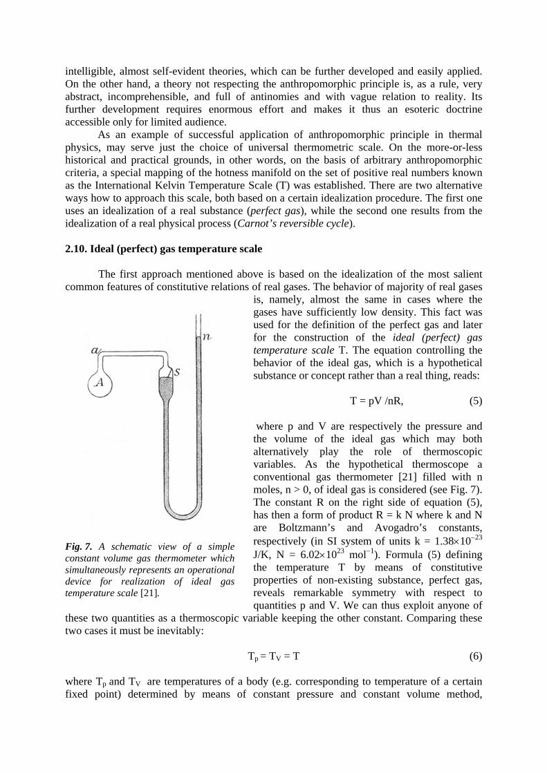
intelligible, almost self-evident theories, which can be further developed and easily applied. On the other hand, a theory not respecting the anthropomorphic principle is, as a rule, very abstract, incomprehensible, and full of antinomies and with vague relation to reality. Its further development requires enormous effort and makes it thus an esoteric doctrine accessible only for limited audience.

As an example of successful application of anthropomorphic principle in thermal physics, may serve just the choice of universal thermometric scale. On the more-or-less historical and practical grounds, in other words, on the basis of arbitrary anthropomorphic criteria, a special mapping of the hotness manifold on the set of positive real numbers known as the International Kelvin Temperature Scale (T) was established. There are two alternative ways how to approach this scale, both based on a certain idealization procedure. The first one uses an idealization of a real substance (perfect gas), while the second one results from the idealization of a real physical process (Carnot’s reversible cycle).

2.10. Ideal (perfect) gas temperature scale

The first approach mentioned above is based on the idealization of the most salient

common features of constitutive relations of real gases. The behavior of majority of real gases is, namely, almost the same in cases where the gases have sufficiently low density. This fact was used for the definition of the perfect gas and later for the construction of the ideal (perfect) gas temperature scale T. The equation controlling the behavior of the ideal gas, which is a hypothetical substance or concept rather than a real thing, reads:

T = pV /nR, (5)

where p and V are respectively the pressure and the volume of the ideal gas which may both alternatively play the role of thermoscopic variables. As the hypothetical thermoscope a conventional gas thermometer [21] filled with n moles, n > 0, of ideal gas is considered (see Fig. 7). The constant R on the right side of equation (5), has then a form of product R = k N where k and N are Boltzmann’s and Avogadro’s constants, respectively (in SI system of units k = 1.38×10−23 J/K, N = 6.02×1023 mol−1). Formula (5) defining the temperature T by means of constitutive properties of non-existing substance, perfect gas, reveals remarkable symmetry with respect to quantities p and V. We can thus exploit anyone of

these two quantities as a thermoscopic variable keeping the other constant. Comparing these two cases it must be inevitably:

Fig. 7. A schematic view of a simple constant volume gas thermometer which simultaneously represents an operational device for realization of ideal gas temperature scale [21].

Tp = TV = T (6)

where Tp and TV are temperatures of a body (e.g. corresponding to temperature of a certain fixed point) determined by means of constant pressure and constant volume method,

respectively. The exact realization of condition (6) in experiments with real gases and with prescribed high accuracy (typically of order of 0.1%) is very difficult if not impossible. However, Berthelot [22] devised a simple mathematical method based on plausible assumptions which enables to extrapolate experimental data obtained on real gases at finite pressures to the case corresponding to the ideal gas and finally determine also the value of T satisfying conditions (6). From these facts it is thus apparent that the ideal gas temperature scale can be experimentally realized in the range where the gaseous phase of real gases exists. 2.11. Absolute temperature

The ideal gas temperature scale T defined by means of equation (5) has some other remarkable properties. For example, as both quantities p and V have a natural lower bound equal to zero, the temperature T has also this lower bound. In this connection it is interesting to mention considerations of French savant G. Amontons (1703) [23,24] who made extensive experiments with constant volume gas thermometer filled with dry air. By means of extrapolation of a regular “centigrade” temperature scale, constructed between boiling and freezing points of water, down to the zero pressure he obtained a value of −240°C (contemporary measurements would provide the value near −273°C). As for him it was absolutely inconceivable that the temperature of any body in the Universe could decrease below the point in which the activity of such a “vivacious” substance as the air disappears, he started to call this hypothetical temperature l’extrêm froid. Interestingly, quite independently but on the basis of similar experiments, introduced absolute zero of temperature (zéro absolu de la chaleur) also Clément and Désormes [25]. Nevertheless, not diminishing huge merits of these distinguished men of science, their considerations were not correct in principle. Indeed, as was already mentioned, every thermoscope enables to order the thermoscopic states only locally, within a certain well-defined range. The extrapolations out of this range are not permissible. Moreover, technical collapse of a particular type of thermoscope (e.g. due to the freezing of air in its bulb) cannot serve as a proof for non-existence of other types of thermoscopes possibly working at lower temperatures. On the other hand the definition of temperature gives us a sufficient freedom to introduce the scale with absolute zero not on the basis of some recognized “Law of Nature” but simply on the basis of our decision. Such a scale, namely, may have besides compatibility with equation (5) some advantages, e.g. numerous problems with sign can be avoided, the evaluation of integrals depending on temperature is simplified etc. The definition of absolute temperature4 scale then reads [20]:

Any temperature scale which is chosen in such a way that their functional values have

highest lower bound equal to zero (i.e. T is always positive), is called absolute temperature scale and the corresponding temperatures are called absolute temperatures.

Notice that the possible value T = 0 (equal to highest lower bound) is already excluded by

our definition of temperature, because due to the absence of the lowest hotness level in the hotness manifold any continuous one-to-one order-preserving transformation on the set with lower bound = 0, has inevitably to map its improper point (i.e. – ∞ ) just on the point corresponding to absolute zero. Nernst’s law of unattainability of absolute zero of temperature (“Third Law of Thermodynamics”) [26] is thus together with its consequences intrinsically

4 Notice that this definition of absolute temperature scale differs from that due to Lord Kelvin who related the adjective “absolute” rather to the independence of temperature scale of thermometric substance than to the existence of lower bound of temperature values.

involved in this definition of temperature and, consequently, needs no additional, sometimes very curious, justifications or “proofs” [27]. 2.12. Carnot’s theorem

Reasonably chosen temperature function which maps the hotness manifold on a subset of real numbers should be, as was already mentioned in paragraph 2.2., conformal with other terms entering the energy balance equation. In such a case will temperature (intensive quantity, T) and heat (extensive quantity, ς) make up a couple of conjugate variables obeying dimensional equation (1) i.e. [Energy] = [T ] × [ς ].

The principal possibility to write down the thermal energy term just in this form was confirmed by early experiments on the development of mechanical work by means of heat engines. In spite of the fact that these experiments were backed by a rather primitive technique (e.g. temperatures were measured by roughly calibrated mercury thermometers and heat by the weight of burned coal) being thus of doubtful accuracy, their analysis enabled S. Carnot to introduce some new theoretical concepts and draw out definite conclusions. In the present context play among new Carnot’s concepts the most important roles two idealizations of real thermal process taking place in the heat engine, namely, the cyclic process and reversible process. By cyclic process (cycle) is meant any thermal process in which initial and final physical state of the heat engine are the same. The reversible process is then a thermal process in which heat engine works without wastes of heat. For heat engines utilizing the cyclic reversible process (so called ideal heat engines) was Carnot able to formulate a theorem which in its archaic version reads5 [28]

“The motive power of heat is independent of the agents set at work to realize it; its quantity is fixed solely by the temperatures of the bodies between which, in the final result, the transfer of caloric is done.” (S. Carnot, 1824)

Of course, from the modern point of view is Carnot’s theorem rather a desideratum than piece of scientific knowledge. (Remarkable is also a somewhat inconsistent use of heat and caloric as synonyms!) On the other hand, it has a form of the energy balance postulate we are searching for. Indeed, if we, namely, transform the theorem into mathematical symbols we can write it in terms of finite differences [29]

ΔL = ς F’(t) Δt , (8) where ς means the quantity of heat regardless of the method of its measurement, ΔL is the motive power (i.e. useful work done by heat engine) and Δt is the difference between empirical temperatures of heater and cooler. The unknown dimensionless function F’(t) called Carnot’s function should be for concrete empirical scale determined by experiment. As the 5 It should be stressed here that there can be found in the literature a lot of various arbitrarily changed forms of “Carnot’s theorem” or “principle” which are not equivalent one to each other and which essentially differs in their very content from the original formulation. As was thus quite correctly pointed out by distinguished researcher into the vapour turbines and president of Royal Society, H. L. Callendar [29], the original oldest Carnot’s formulation of his principle is at the same time the best one.

gained work ΔL has a dimension of energy and as this energy must be for reversible cycle equal per definition to the thermal energy of heat ς supplied to the ideal heat engine, we can conclude that the terms suitable for insertion into the energy balance equation have to have a form of products ςΔt properly modified by Carnot’s function. 2.13. Kelvin’s proposition A revolutionary step toward the definition of temperature scale independent of particular type of thermometer and thermometric substance was made at 1848 by Lord Kelvin [30]. He proposed to treat Carnot’s theorem not as a heuristic statement deduced from experiments of rather a limited accuracy but as a fundamental postulate of absolute validity. He further pointed out that the very purpose of Carnot’s function is to modify or correct the difference of temperatures measured in a particular empirical temperature scale in such a way that it could serve as a exact proportionality factor between work, ΔL, and heat, ς. As this factor has to be according to Carnot’s postulate the same for all substances, Kelvin, inverting the logics of reasoning, suggested to define a universal (in his terminology “absolute”, see footnote 4) temperature scale just by prescribing a proper analytical form of Carnot’s function. For example, giving to Carnot’s function the simplest permissible analytical form, namely, F’(*T) = 1 (so called caloric gauge6) we are in fact defining a new temperature scale *T in terms of which equation (7) reads: ΔL = ς (*T2 −*T1). (9)

It is immediately seen that using such a definition of temperature scale the energy terms have the desired form of a product of two conjugate variables ς and *T. Interestingly enough, equation (10) is simultaneously a fundamental relation of caloric theory of heat (cf. [31]). Accordingly, the heat is from phenomenological point of view a kind of substance or fluid, caloric (calorique, Wärmestoff, теплородъ, teplík), which being dissolved in all bodies is responsible for their thermal state. It is treated as an indestructible fluid (recall that the only method how to get rid of heat is to convey it away), which is created in every irreversible processes such as rubbing, chemical reactions, burning, absorption of radiation and eating during which “something” simultaneously disappears for ever. The properties of so defined quantity are thus very near to the concept of heat in a common sense [32,33]. Taking further into account the structure of equation (9) we can also conclude that the development of moving force in an ideal heat engine is not connected with some actual consumption of heat as is claimed in thermodynamics but rather with its transfer from hotter body to a colder one (water-mill analogy [28]). At the same time equation (9) defines an entropy-like unit of heat fully compatible with the SI system which may be, according to Callendar’s suggestion, appropriately called “Carnot” (Abbreviation “Ct”) [29]. 1 Ct is then that quantity of heat which is in a reversible process capable of producing 1 J of work per 1 K temperature fall.

In the present context is, nevertheless, far more important another aspect of equation (9). Accordingly, namely, the temperature difference *T2 −*T1 between two bodies used e.g. as “heater” and “cooler” of an ideal heat engine, is identical with the ratio ΔL/ς where both of

6 Due to the later general acceptance of Joule-Mayer’s postulate claiming the equivalence of work and heat it was no more possible to choose freely Carnot’s function which had inevitably the form J/T (thermodynamics’ gauge), where J is so called mechanical equivalent of heat [31]. Fortunately, this fact does not influence our further considerations but rather gives an opportunity to the exercise in elementary algebra interpreted in textbooks as a “proof” of mechanical origin of the Kelvin temperature scale.

these quantities are measurable in principle; ΔL by means of standard methods well-known from mechanics and ς e.g. by amount of fuel consumed by heating the heater or, if the cooler is kept at 0 °C, by amount of ice melted during the cycle. It is quite obvious that such a technique of temperature measurement, although possible in principle, is rather a curiosum which would be very difficult to realize with sufficiently high accuracy in practice. The idea of this method is, however, of primary importance for theory. Obviously, due to Carnot’s postulate equation (9) has to be valid for any ideal heat engine regardless of its construction and working substance used. Analyzing thus one representative case of ideal heat engine general conclusions can be made. For example, if we imagine an ideal heat engine driven by perfect gas and working in cycles which consist of two isothermal and two isochoric reversible processes, the useful work can be easily computed, provided that the temperatures are measured in terms of perfect gas scale. The result of such a computation reads

ΔL = nR ln(V2/V1) (T2 − T1), (10)

where V1 and V2 are limits of volume between which the engine operates. It is apparent at first glance that this last equation is fully congruent with equation (9) with the proviso that the heat (measured in entropy units, e.g. Ct) transferred from heater to cooler per cycle is given by ς = nR ln(V2/V1). The congruence of these equations means that the system of units can be always chosen in such a way that scales *T and T will be identical [6]. Expressing this fact more physically we can say:

Measurement of temperatures by means of ideal gas thermometer is equivalent to the measurement of temperatures by means of ideal heat engine.

The theoretical significance of this theorem is enormous because it enables one to

relate without ambiguity the ideal gas (Kelvin) temperature scale to the temperatures defined by other types of ideal heat engines e.g. “gedanken” reversible cycles in systems controlled by electric, magnetic or electrochemical forces. Besides, it should be stressed that this theorem, although it is based on arbitrary assumptions, is by no means accidental. The idealization of constitutive relation of real gases and idealisation involved in Carnot’s postulate have the same anthropomorphic roots, namely, the feeling that the thermal dilatation of bodies must be linearly dependent on their thermal state. Incidentally, in the range between 0°C and 100°C are the air scale and the mercury temperature scale, prevailingly used in experiments related to establishment of Carnot’s theorem, almost identical.

2.14. Scholion

The concept of fundamental quantity of thermal physics, temperature, is defined as an

arbitrary one-to-one order preserving continuous mapping of so-called hotness manifold on a certain simple connected open subset of real numbers. The hotness manifold H representing all in the Nature existing thermoscopic (thermal) states is the only entity accessible to direct physical observation. The set H, which was proved to be topologically equivalent to the set of all real numbers (real axis), contains a countable, dense and unbounded subset of all fixed points F ⊂ H. Any fixed point is realized by means of a specially prepared body which defines just one thermal state. The properties of set F and its relation to the manifold H are specified by means of Mach’s postulates. As has been finally shown, the special mapping of H on the set of all positive real numbers known as the International Kelvin Temperature Scale T was chosen on the grounds of two anthropomorphic idealizations providing a concordant result, namely, ideal substance, perfect gas and ideal process in heat engine, reversible cycle.

Acknowledgement The present work was supported by Institutional Research Plan of Institute of Physics ASCR v.v.i. No AV0Z10100521. References [1] Giua M.: Storia della chimica. Union Tipografico, Torino (1962), Russian transl. Dzhua

M.: Istoriya Chimii. Izdatel’stvo Mir, Moscow (1975) [2] Meyer-Bjerrum K.: Die Entwicklung des Temperaturbegriffs im Laufe der Zeiten.

Vieweg und Sohn, Braunschweig (1913) [3] Burckhardt F.: Die Erfindung des Thermometers und seine Gestaltung im XVII

Jahrhundert. Basel (1867) [4] Black J.: Lectures on the Elements of Chemistry. W. Creech, Edinburgh (1803), Germ.

transl.: Vorlesungen über Chemie. Crell, Hamburg (1804) [5] Fürth R.: Algemeine Grundlagen der Physik, Prinzipien der Statistik. In: Handbuch der

Physik Bd. IV. Springer, Berlin (1929) [6] Palacios J.: Dimensional Analysis. Macmillan & Co. Ltd., London (1964) [7] Balamuth L., Wolfe H. C., Zemansky M. W.: The Temperature Concept from the

Macroscopic Point of View. Am. J. Phys. 9, 199 (1941) [8] Boas M.: Hero’s Pneumatica, A Study of its Transmission and Influence. Isis 40, 38

(1949) [9] Hoppe E.: Geschichte der Physik. F. Vieweg und Sohn, a.G., Braunschweig (1926) [10] Fludd R.: Mosaical Philosophy. H. Moseley, London (1659) [11] Mach E.: Die Principien der Wärmelehre. Verlag von J. A. Barth, Leipzig (1896) [12] Saggi di naturali sperienze fatte nel’Accademia del Cimento, Firenze (1667) [13] R. Hooke R.: Micrographia. Roy. Soc. of London, Brouncker imprimatur, London

(1665), Reprint: Dover Publications, Inc., Mineola (2003) [14] Boyer C. B.: Early Principles in the Calibration of Thermometers. Am. J. Phys. 10, 176

(1942) [15] A. J. von Oettingen A. J.: Abhandlungen über Thermometrie von Fahrenheit, Réaumur,

Celsius. Ostwald’s Klassiker No.57, W. Engelmann, Leipzig (1894) [16] Barnett M. K.: The Development of Thermometry and the Temperature Concept. Osiris

12, 269 (1956) [17] Fahrenheit D. G.: Experiments and observations on the Freezing of Water in Vacuuo.

Phil. Trans. Abridged 33, 22 (1724) [18] Huntington E. V.: The Continuum and Other Types of Serial Order. Harvard University

Press, New York (1917), Reprint: Dover Phoenix Editions, New York (2003) [19] Hilbert D.: Über das Unendliche. Math . Ann. 95, 161 (1926) [20] Truesdell C., Bharatha S.: Concepts and Logic of Classical Thermodynamics as a

Theory of Heat Engines. Springer, New York (1977) [21] Nieto A., Paul F.: Mesure des Températures. Éditions Radio, Paris (1958) [22] Wensel H. T.: Temperature and Temperature Scales. J. Appl. Phys. 11, 373 (1940) [23] Brush S. G.: The Kind of Motion We Call Heat. North-Holland, Amsterdam (1976) [24] Amontons G.: Le Thermométre. Mémoires de l’Académie Royale des Sciences 6, 64

(1703)

[25] Clément C. B., Désormes N.: Détermination expérimentale du zéro absolu de la chaleur et du calorique spécifique des gaz. Journal de physique 89, 321,428 (1819)

[26] Nernst W.: The New Heat Theorem. (1926) Reprint: Dover Publications, Inc., New York (1969)

[27] Boas M. L.: A Point of Logic. Am. J. Phys. 28, 675 (1960) [28] Carnot S.: Réflexions sur la puissance motrice du feu et sur les machines propres à

développer cette puissance. Bachelier, Paris (1824), Germ. transl.: Ostwald’s Klassiker, Nr. 37, Egelmann, Leipzig (1909)

[29] Callendar H. L.: The Caloric Theory of Heat and Carnot’s Principle. Proc. Phys. Soc. London 23, 153 (1911)

[30] Thomson W. (Lord Kelvin of Largs): On the Absolute Thermometric Scale founded on Carnot’s Theory of the Motive Power of Heat. Phil. Mag. 33, 313 (1848)

[31] Mareš J. J., Hubík P., Šesták J., Špička V., Krištofik J., Stávek J.: Phenomenological approach to the caloric theory of heat. Thermochimica Acta 474, 16 (2008)

[32] Job G.:Neudarstellung der Wärmelehre – Die Entropie als Wärme. Akad. Verlagsges., Frankfurt am Main (1972)

[33] Falk G., Herrmann F., Schmid G. B.: Energy Forms or Energy Carriers? Am. J. Phys. 51, 1074 (1983)