quantifquantile : an r package for performing quantile...

CONTRIBUTED RESEARCH ARTICLE 1

QuantifQuantile : an R Package forPerforming Quantile Regression throughOptimal Quantizationby Isabelle Charlier, Davy Paindaveine and Jérôme Saracco

Abstract In quantile regression, various quantiles of a response variable Y are modelled as func-tions of covariates (rather than its mean). An important application is the construction of referencecurves/surfaces and conditional prediction intervals for Y. Recently, a nonparametric quantile regres-sion method based on the concept of optimal quantization was proposed. This method competes verywell with k-nearest neighbor, kernel, and spline methods. In this paper, we describe an R package,called QuantifQuantile, that allows to perform quantization-based quantile regression. We describethe various functions of the package and provide examples.

Introduction

In numerous applications, quantile regression is used to evaluate the impact of a d-dimensionalcovariate X on a (scalar) response variable Y. Quantile regression is an interesting alternative tostandard regression whenever the conditional mean does not provide a satisfactory picture of theconditional distribution. Denoting by F(·|x) the conditional distribution of Y given X = x, theconditional quantile functions

x 7→ qα(x) = inf {y ∈ R : F(y|x) ≥ α} , α ∈ (0, 1), (1)

indeed always yield a complete description of the conditional distribution. For our purposes, it isuseful to recall that the conditional quantiles in (1) can be equivalently defined as

qα(x) = arg mina∈R

E[ρα(Y− a)|X = x], (2)

where ρα(z) = αzI[z≥0] − (1− α)zI[z<0] is the so-called check function.

For fixed α, the quantile functions x 7→ qα(x) provide reference curves (when d = 1), one for eachvalue of α. For fixed x, they provide conditional prediction intervals of the form Iα = [qα(x), q1−α(x)](α < 1/2). Such reference curves and prediction intervals are widely used, e.g. in economics, ecology,or lifetime analysis. In medicine, they are used to provide reference growth curves for children’sheight and weight given their age.

Many approaches have been developed to estimate conditional quantiles. After the seminalpaper of Koenker and Bassett (1978) that introduced linear quantile regression, much effort has beenmade to consider nonparametric quantile regression. The most classical procedures in this vein arethe nearest neighbor estimators (Bhattacharya and Gangopadhyay, 1990), the (kernel) local linearestimators (Yu and Jones, 1998) or the spline-based estimators (Koenker et al., 1994; Koenker andMizera, 2004). For related work, we also refer to, e.g. Fan et al. (1994), Gannoun et al. (2002), Muggeoet al. (2013) and Yu et al. (2003). There also exists a wide variety of R functions/packages dedicated tothe estimation of conditional quantiles. Among them, let us cite the functions rqss (only for d ≤ 2) andgcrq (only for d = 1) from the packages quantreg (Koenker, 2013) and quantregGrowth (Muggeo,2014), respectively.

Recently, Charlier et al. (2015a) proposed a nonparametric quantile regression method based on theconcept of optimal quantization. Optimal quantization replaces the (typically continuous) covariate Xwith a discretized version XN obtained by projecting X on a collection of N points (these N points,that form the quantization grid, are chosen to minimize the Lp-norm of X− XN ; see below). As shownin Charlier et al. (2015b), the resulting conditional quantile estimators compete very well with theirclassical competitors.

The goal of this paper is to describe an R package, called QuantifQuantile (Charlier et al., 2015c),that allows to perform quantization-based quantile regression. This includes the data-driven selectionof the grid size N (that plays the role of a tuning parameter), the construction of the correspondingquantization grid, the computation of the resulting sample conditional quantiles, as well as (for d ≤ 2)their graphical representation.

The paper is organized as follows. The first section briefly recalls the construction of quantization-based quantile regression introduced in Charlier et al. (2015a,b) and explains the various steps neededto obtain the resulting estimators. The second section lists the main functions of QuantifQuantile and

The R Journal Vol. XX/YY, AAAA ISSN 2073-4859

http://CRAN.R-project.org/package=quantreg

http://CRAN.R-project.org/package=quantregGrowth

http://CRAN.R-project.org/package=QuantifQuantile


describes their inputs and outputs. Finally, the third section provides several examples that illustratethe use of the various functions. We conclude the paper by comparing our method with R alternativeson a real data set. An illustration of the function computing optimal quantization grids is given inthe Appendix, which can be of independent interest in numerical probability, finance or numericalintegration where quantization is extensively used (Pagès, 1998; Pagès et al., 2004)).

Quantile regression through quantization

As mentioned above, the R package we describe in this paper implements the Charlier et al. (2015a,b)quantization-based methodology to perform nonparametric quantile regression. This section describesthis methodology.

Approximating population conditional quantiles through quantization

Let γN ∈ (Rd)N be a grid of size N, that is, a collection of N points in Rd. For any x ∈ Rd, we willdenote by xγN

= ProjγN (x) the projection of x onto this grid, that is, the point of γN that is closest to x(absolute continuity assumption makes ties unimportant in the sequel). This allows to approximatethe d-dimensional covariate X by its quantized version XγN

.

Obviously, the choice of the grid has a significant impact on the quality of this approximation.Under the assumption that ‖X‖p := E[|X|p]1/p < ∞ (throughout, | · | denotes the Euclidean norm),optimal quantization selects the grid γN that minimizes the Lp-quantization error ‖X− XγN‖p. Suchan optimal grid exists under the assumption that the distribution PX of X does not charge anyhyperplane, i.e. under the assumption that PX [H] = 0 for any hyperplane H (Pagès, 1998). In practice,an optimal grid is constructed using a stochastic gradient algorithm (see the following section). For moredetails on quantization, the reader may refer to Pagès (1998) and Graf and Luschgy (2000).

Based on optimal quantization of X, we can approximate the conditional quantile qα(x) in (2) by

qNα (x) := arg min

a∈RE[ρα(Y− a)|XN = xN], (3)

where XN (resp., xN) denotes the projection of X (resp., x) onto an optimal grid. It is shown in Charlieret al. (2015a) that – under mild assumptions,1 qN

α (x) converges to qα(x) as N → ∞, uniformly in x.

Obtaining an optimal N-grid

As we will see below, whenever independent copies (X′1, Y1)′, . . . , (X′n, Yn)′ of (X′, Y)′ are available,

the first step to obtain a sample version of (3) is to compute an optimal N-grid (we assume here thatN is fixed). As already mentioned, this can be done through a stochastic gradient algorithm. Thisalgorithm, called Competitive Learning Vector Quantization (CLVQ) when p = 2, is an iterative procedurethat operates as follows :

• First, an initial grid — γN,0, say — is chosen by sampling randomly without replacement amongthe Xi’s.

• Second, n iterations are performed (one for each observation available). The grid γN,t =

(γN,t1 , . . . , γN,t

N ) at step t is obtained through

γN,ti =

{γN,t−1

i − δt|γN,t−1i − Xt|p−1 γN,t−1

i −Xt

|γN,t−1i −Xt |

if ProjγN,t−1 (Xt) = γN,t−1i ,

γN,t−1i otherwise,

where (δt), t ∈N0, is a deterministic sequence in (0, 1) such that ∑t δt = ∞ and ∑t δ2t < ∞. At

the tth iteration, only one point of the grid moves, namely the one that is closest to Xt.

The optimal grid provided by this algorithm is then γN,n.

Estimating conditional quantiles

Assume now that a sample (X′1, Y1)′, . . . , (X′n, Yn)′ as above is indeed available. The sample analog

of (3) is then defined as follows :1Our method actually requires assumptions on the link function between Y and X and on the error term of the

model. These assumptions in particular guarantee that, for any x, the conditional distribution of Y given X = x isabsolutely continuous; we refer to Charlier et al. (2015a) for details.



(S1) First, we compute the optimal grid γN,n through the stochastic gradient algorithm just described,and we write XN

i = ProjγN,n (Xi), i = 1, . . . , n.

(S2) Then, the conditional quantiles are estimated by

qN,nα (x) = arg min

a∈R

n

∑i=1

ρα(Yi − a)I[XNi =xN ], (4)

where xN = ProjγN,n (x). In practice, qN,nα (x) is simply evaluated as the sample α-quantile of the

Yi’s for which XNi = xN .

It is shown in Charlier et al. (2015a) that – under mild assumptions, qN,nα (x), for any fixed N and x,

converges in probability to qNα (x) as n→ ∞, provided that quantization is based on p = 2.

When the sample size n is small to moderate (n ≤ 300, say), the estimated reference curves x 7→qN,n

α (x) typically are not smooth. To improve on this, Charlier et al. (2015a,b) introduced the followingbootstrapped version of the estimator in (4). For some positive integer B, generate B samples of size nfrom the original sample {(X′i , Yi)

′}i=1,...,n with replacement. From each of these bootstrap samples,the stochastic gradient algorithm provides an "optimal" grid, using these bootstrapped samples toperform the iterations. The bootstrapped estimator of conditional quantile is then

qN,nα,B (x) =

1B

B

∑b=1

q(b)α (x), (5)

where q(b)α (x) = q(b),N,nα (x) denotes the estimator in (4) computed on the basis of the bth optimal grid.

We stress that, when computing q(b)α (x), the original sample is used in (S2); the bootstrapped samplesare only used to provide the B different grids. As shown in Charlier et al. (2015a,b), the bootstrappedreference curves are much smoother than the original ones. Of course, B should be chosen largeenough to make the bootstrap useful, but also small enough to keep the computational burden undercontrol. For d = 1, we usually choose B = 50.

Selecting the grid size N

Both for the original estimators qN,nα (x) and for their bootstrapped versions qN,n

α,B (x), an appropriatevalue of N should be identified. If N is too small, then reference curves will have a large bias, while ifN is too large, then they will show much variability. This leads to the usual bias/variance trade-offthat is to be achieved when selecting the value of a smoothing parameter in nonparametric statistics.

Charlier et al. (2015b) proposed the following data-driven method to choose N. Let {x1, . . . , xJ}be a set of x-values at which we want to estimate qα(x) (the xj’s are for instance chosen equispacedon the support of X) and let N be a finite collection of N-values (this represents the values of N oneallows for and should typically be chosen according to the sample size n). Ideally, we would like toselect the optimal value of N as

N¯α;opt = arg min

N∈NISE¯

α(N), with ISE¯α(N) =

1J

J

∑j=1

(qN,n

α,B (xj)− qα(xj))2. (6)

This, however, is infeasible, since the population quantiles qα(xj) are unknown. This is why we drawB extra bootstrap samples (still of size n) from the original sample and consider

N¯α;opt = arg min

N∈NISE

¯α(N), with ISE

¯α(N) =

1J

J

∑j=1

(1B

B

∑b=1

(qN,n

α,B (xj)− q(b)α (xj))2)

, (7)

where q(b)α (xj), for b = 1 . . . , B, makes use of this bth new bootstrap sample; more precisely, thebootstrap sample is still only used to perform the iterations of the algorithm, whereas the originalsample is used in both the initial grid and in (S2).

As shown in Charlier et al. (2015b) through simulations, both N 7→ ISE¯α(N) and N 7→ ISE

¯α(N) are

essentially convex in N and lead to roughly the same minimizers. This therefore provides a feasibleway to select a reasonable value of N for the estimator qN,n

α,B (x) in (5). Note that this also applies

to qN,nα (x) by simply taking B = 1 in the procedure above.

If quantiles are to be estimated at various orders α, (7) will provide an optimal N-value for each α. Itmay then happen, in principle, that the resulting reference curves cross, which is of course undesirable.



One way to guarantee that no such crossings occur is to identify a common N-value for the various α’s.In such a case, N will be chosen as

N¯opt = arg min

N∈NISE

¯(N), with ISE

¯(N) = ∑α ISE

¯α(N), (8)

where the sum is computed over the various α-values considered.

Charlier et al. (2015b) performed extensive comparisons between the quantization-based estimatorsin (5) — based on the efficient data-driven selection method for N just described — and some of theirmain competitors, namely estimators obtained from spline, k-nearest neighbor, and kernel methods.This revealed that the quantization-based estimators compete well in all cases, and often dominatestheir competitors (in terms of integrated square errors), particularly so for complex link functions; seeCharlier et al. (2015b) for details.

Unlike the local linear and local constant estimators from Yu and Jones (1998), that are usuallybased on a global-in-x bandwidth, our quantization-based estimators are locally adaptive in the sensethat, when estimating qα(x), the "working bandwidth" — that is, the size of the quantization cellcontaining x — depends on x. The k-nearest neighbor (kNN) estimator is closer in spirit to quantization-based estimators but always selects k neighbors, irrespective of the x-value considered, whereas thenumber of Xi’s in the quantization cell of x may depend on x. This subtle local-in-x behavior mayexplain the good empirical performances of quantization-based estimators over kernel and nearest-neighbor competitors. Finally, spline methods (implemented in R with the rqss and qss functions)tend to perform poorly for complex link functions, since they always provide piecewise linear referencecurves (Koenker et al., 1994). Moreover, the current implementation of the rqss function only supportsdimensions 1 and 2, whereas our package allows to compute quantization-based estimators in anydimension d.

The QuantifQuantile package

This section provides a description of the various functions offered in the R package QuantifQuantile.We first detail the three functions that allow to estimate conditional quantiles through quantization.Then we describe a function computing optimal quantization grids.

Conditional quantile estimation

QuantifQuantile is composed of three main functions that each provide estimated conditional quan-tiles in (4)-(5). These functions work in a similar way but address different values of d (recall that d isthe dimension of the covariate vector X) :

• The function QuantifQuantile is suitable for d = 1.

• The function QuantifQuantile.d2 addresses the case d = 2.

• Finally, QuantifQuantile.d can deal with an arbitrary value of d.

Combined with the plot function, the first two functions provide reference curves and referencesurfaces, respectively. No graphical outputs can be obtained from the third function if d > 2.

The three functions share the same arguments, but not necessarily the same default values. Foreach function, using args() displays the various arguments and corresponding default values :

> args(QuantifQuantile)

function(X, Y, alpha = c(0.05, 0.25, 0.5, 0.75, 0.95), x = seq(min(X), max(X),length = 100), testN = c(35, 40, 45, 50, 55), p = 2, B = 50, tildeB = 20,same_N = TRUE, ncores = 1)

> args(QuantifQuantile.d2)

function(X, Y, alpha = c(0.05, 0.25, 0.5, 0.75, 0.95), x = matrix(c(rep(seq(min(X[1, ]),max(X[1, ]), length = 20), 20), sort(rep(seq(min(X[2, ]), max(X[2, ]), length =20), 20))), nrow = 2, byrow = TRUE), testN = c(110, 120, 130, 140, 150), p = 2,B = 50, tildeB = 20, same_N = TRUE, ncores = 1)

> args(QuantifQuantile.d)



function(X, Y, x, alpha = c(0.05, 0.25, 0.5, 0.75, 0.95), testN = c(35, 40, 45, 50, 55),p = 2, B = 50, tildeB = 20, same_N = TRUE, ncores = 1)

We now give more details on these arguments.

• X: a d× n real array (required by all three functions, a vector of length n for QuantifQuantile).The columns of this matrix are the Xi’s, i = 1, . . . , n.

• Y: an n× 1 real array (required by all three functions). This vector collects the Yi’s, i = 1, . . . , n.

• alpha: an r× 1 array with components in (0, 1) (optional for all three functions). This vectorcontains the orders for which qα(x) should be estimated.

• x: a d × J real array (optional for QuantifQuantile and QuantifQuantile.d2, required byQuantifQuantile.d). The columns of this matrix are the xj’s at which the quantiles qα(xj)are to be estimated. If x is not provided when calling QuantifQuantile, then it is set to avector of J = 100 equispaced values between the minimum and the maximum of the Xi’s. Ifthis argument is not provided when calling QuantifQuantile.d2, then the default for x is amatrix whose J = 202 = 400 column vectors are obtained as follows: 20 equispaced values areconsidered between the minimum and maximum values of the (Xi)1’s and similarly for thesecond component. The 400 column vectors of the default x are obtained by considering allcombinations of those 20 values for the first component with the 20 values for the second one2.

• testN: an m× 1 vector of pairwise distinct positive integers (optional for all three functions).The entries of this vector are the elements of the set N in (7)-(8), hence are the N-values forwhich the ISE

¯α quantity considered will be evaluated. The default is (35, 40, . . . , 55) but it is

strongly recommended to adapt it according to the sample size n at hand.

• p: a real number larger than or equal to one (optional for all three functions). This is theparameter p to be used when performing optimal quantization in Lp-norm.

• B: a positive integer (optional for all three functions). This is the number of bootstrap replicationsB to be used in (5).

• tildeB: a positive integer (optional for all three functions). This is the number of bootstrapreplications B to be used when determining N¯

α;opt or N¯opt.

• same_N: a boolean variable (optional for all three functions). If same_N=TRUE, then a commonvalue of N (that is, N¯

opt in (8)) will be selected for all α’s. If same_N=FALSE, then optimal valuesof N will be chosen independently for the various of α (which will provide several N¯

α;opt, asin (7)).

• ncores: number of cores to use. These functions can use parallel computation to save time byincreasing this parameter. Parallel computation relies on mclapply from parallel package, henceis not available on Windows.

All three functions return the following list of objects, which is of class "QuantifQuantile" :

• hatq_opt: an r× J real array (where r is the number of α-values considered). If same_N=TRUE,

then the entry (i, j) of this matrix is qN¯

opt,nαi ,B (xj). If same_N=FALSE, then it is rather q

N¯αi ;opt,n

αi ,B (xj).This object can also be returned using the usual fitted.values function.

• N_opt: a positive integer (if same_N=TRUE) or an r× 1 array of positive integers (if same_N=FALSE).Depending on same_N, this provides the value of N¯

opt or the vector (N¯α1;opt, . . . , N¯

αr ;opt).

• hatISE_N: an r×m real array. The entry (i, j) of this matrix is ISE¯αi(Nj). Plotting this for fixed α

or plotting its average over the various α, in both cases over testN, allows to assess the globalconvexity of these ISEs. Hence, it can be used to indicate whether or not the choice of testNwas adequate. This will be illustrated in the examples below.

• hatq_N: an r× J ×m real array. The entry (i, j, `) of this matrix is qN` ,nαi ,B (xj), where N` is the `th

entry of the argument testN. From this output, it is easy by fixing the third entry to get thematrix of the qN,n

αi ,B(xj) values for any N in testN.

• The arguments X, Y, x, alpha, and testN are also reported in this response list.

Moreover, when the optimal value N_opt selected is on the boundary of testN, which means thattestN most likely was not well chosen, a warning message is printed.

The "QuantifQuantile" class response can be used as argument of the functions plot (only ford ≤ 2), summary and print. The plot function draws the observations and plots the estimated

2Since the number J of points in a default value of x obtained in this fashion would increase exponentially withthe dimension d, we did not adopt the same approach for d ≥ 3.


http://CRAN.R-project.org/package=parallel


conditional quantile curves (d = 1) or surfaces (d = 2) — for d = 2, the rgl package is used (Adleret al., 2014), which allows to change the perspective in a dynamic way. In order to illustrate theselection of N, the function plot also has an optional argument ise. Setting this argument to TRUE (thedefault is FALSE), this function, that can be used for any dimension d, provides the plot (against N) ofthe ISE

¯α and ISE

¯quantities in (7) or in (8), depending on the choice same_N=FALSE or same_N=TRUE,

respectively; see the examples below for details. If d ≤ 2, it also returns the fitted quantile curves orsurfaces.

Computing optimal grids

Besides the functions that allow to estimate conditional quantiles and to plot the correspondingreference curves/surfaces, QuantifQuantile provides a function that computes optimal quantizationgrids. This function, called choice.grid, admits the following arguments :

• X: a d× n real array (required). The columns of this matrix are the Xi’s, i = 1, . . . , n, for whichthe optimal quantization grid should be determined. Each point of X is used as a stimulus in thestochastic gradient algorithm to get an optimal grid.

• N: a positive integer (required). The size of the desired quantization grid.

• ng: a positive integer (optional). The number of desired quantization grids. The default is 1.

• p: a real number larger than or equal to one (optional). This is the parameter p used in thequantization error. The default is 2.

In some cases, it may be necessary to have several quantization grids, such as in (5), where B +tildeB grids are needed. The three functions computing quantization-based conditional quantilesthen call the function choice.grid with ng > 1. In such case, the various grids are obtained using asstimuli a resampling version of X (the Xt’s in the previous section).

The output is a list containing the following elements :

• init_grid: a d×N×ng real array. The entry (i, j, `) of this matrix is the ith component of the jth

point of the `th initial grid.

• opti_grid: a d×N×ng real array. The entry (i, j, `) of this matrix is the ith component of the jth

point of the `th optimal grid provided by the algorithm.

Illustrations

In this section, we illustrate on several examples the use of the functions described above. Examples 1-3restrict to QuantifQuantile/QuantifQuantile.d2 and provide graphical representations in each case.Example 4 deals with a three-dimensional covariate, without graphical representation. An illustrationof the function choice.grid is given in the Appendix.

Example 1 : simulated data with one-dimensional covariate

We generate a random sample (Xi, Yi)′, i = 1, . . . , n = 300, where the Xi’s are uniformly distributed

over the interval (−2, 2) and where the Yi’s are obtained by adding to X2i a standard normal error

term that is independent of Xi :

set.seed(258164)n <- 300X <- runif(n, -2, 2)Y <- X^2 + rnorm(n)

We test the number N of quantizers between 10 and 30 by steps of 5 and we do not changethe default values of the other arguments. We then run the function QuantifQuantile with thesearguments and stock the response in res.

testN <- seq(10, 30, by = 5)res <- QuantifQuantile(X, Y, testN = testN)

No warning message is printed, which means that this choice of testN was adequate. To assess thisin a graphical way, we use the function plot with ise argument set to TRUE that plots hatISEmean_N(obtained by taking the mean of hatISE_N over alpha) against the various N-values in testN.

plot(res, ise = TRUE)


http://CRAN.R-project.org/package=rgl


10 15 20 25 30

0.10

0.11

0.12

0.13

0.14

N

ISE^(N)

(a)

-2 -1 0 1 2

-20

24

6

X

Y

(b)

10 15 20 25 30

0.10

0.11

0.12

0.13

0.14

N

ISE^(N)

(c)

-2 -1 0 1 2

-20

24

6

X

Y

(d)

Figure 1: For the sample considered in Example 1, this figure provides (a) the plot of N 7→ ISE¯(N)

with N ∈ {10, 15, 20, 25, 30}, and (b) the resulting reference curves. The panels (c)-(d) provide thecorresponding plots when taking N ∈ {10, 11, 12, . . . , 19, 20, 25, 30}.

Figure 1a provides the resulting graph, which confirms that testN was well chosen since hatISEmean_Nis larger for smaller and larger values of N than N_opt. We then plot the corresponding estimatedconditional quantiles curves in Figure 1b. The default colors of the points and of the curves arechanged by using the col.plot argument. This argument is a vector of size 1+length(alpha), whosefirst component fixes the color of the data points and whose remaining components determine thecolors of the various reference curves.

col.plot <- c("grey", "red", "orange", "green", "orange", "red")plot(res, col.plot = col.plot, xlab = "X", ylab = "Y")

It is natural to make the grid testN finer. Of course, the more N-values we test, the longer it takes.This is why we adopted this two-stage approach, where the goal of the first stage was to get a roughapproximation of the optimal N-value. In the second stage, we can then refine the grid only in thevicinity of the value N_opt obtained in the first stage.

testN <- c(seq(10, 20, by = 1), seq(25, 30, by = 5))res_step1 <- QuantifQuantile(X, Y, testN = testN)plot(res_step1, ise = TRUE, col.plot = col.plot, xlab = "X", ylab = "Y")

The resulting graphs are provided in Figures 1c-1d, respectively. We observe that the value of N_optis made more precise, since we now get N_opt=18 instead of 15. The resulting estimated conditionalquantiles curves in Figure 1b are very similar to the ones in Figure 1d.



10 15 20 25 30

0.10

0.12

0.14

0.16

N

ISE^α(N)

0.05

0.25

0.5

0.75

0.95

(a)

-2 -1 0 1 2

-20

24

6

X

Y

(b)

10 15 20 25 30

0.08

0.10

0.12

0.14

0.16

0.18

N

ISE^α(N)

0.05

0.25

0.5

0.75

0.95

(c)

-2 -1 0 1 2

-20

24

6

X

Y

(d)

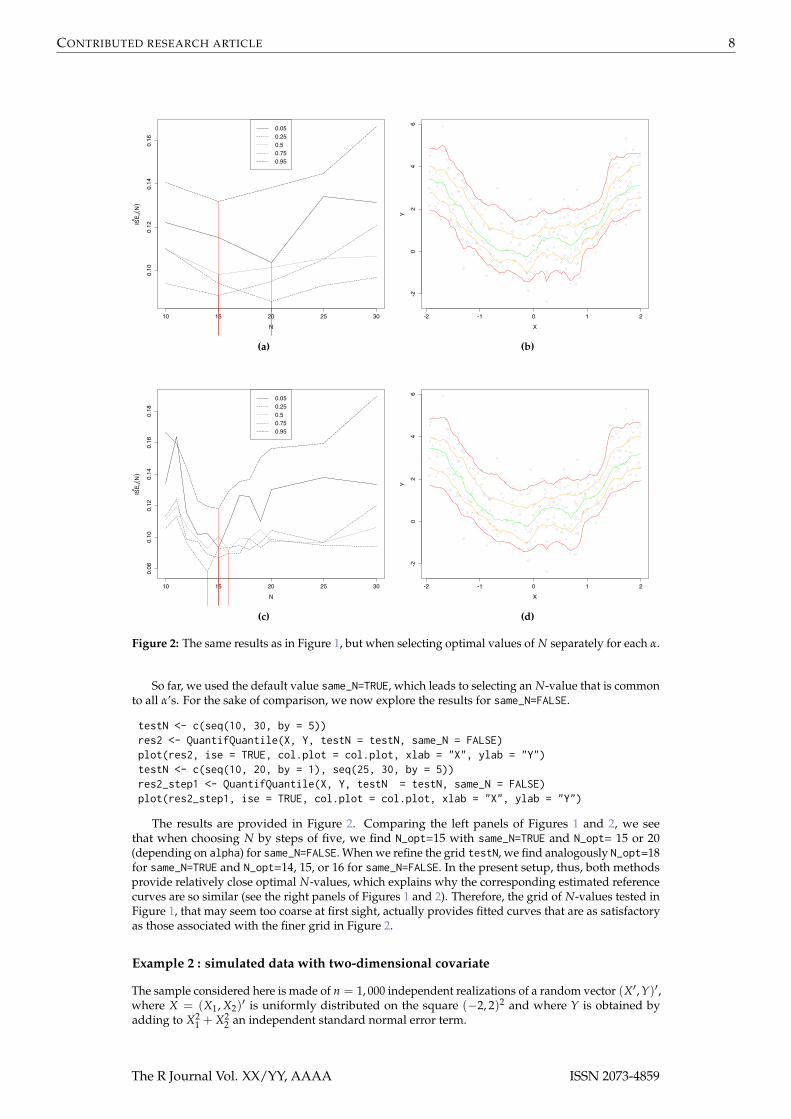
Figure 2: The same results as in Figure 1, but when selecting optimal values of N separately for each α.

So far, we used the default value same_N=TRUE, which leads to selecting an N-value that is commonto all α’s. For the sake of comparison, we now explore the results for same_N=FALSE.

testN <- c(seq(10, 30, by = 5))res2 <- QuantifQuantile(X, Y, testN = testN, same_N = FALSE)plot(res2, ise = TRUE, col.plot = col.plot, xlab = "X", ylab = "Y")testN <- c(seq(10, 20, by = 1), seq(25, 30, by = 5))res2_step1 <- QuantifQuantile(X, Y, testN = testN, same_N = FALSE)plot(res2_step1, ise = TRUE, col.plot = col.plot, xlab = "X", ylab = "Y")

The results are provided in Figure 2. Comparing the left panels of Figures 1 and 2, we seethat when choosing N by steps of five, we find N_opt=15 with same_N=TRUE and N_opt= 15 or 20(depending on alpha) for same_N=FALSE. When we refine the grid testN, we find analogously N_opt=18for same_N=TRUE and N_opt=14, 15, or 16 for same_N=FALSE. In the present setup, thus, both methodsprovide relatively close optimal N-values, which explains why the corresponding estimated referencecurves are so similar (see the right panels of Figures 1 and 2). Therefore, the grid of N-values tested inFigure 1, that may seem too coarse at first sight, actually provides fitted curves that are as satisfactoryas those associated with the finer grid in Figure 2.

Example 2 : simulated data with two-dimensional covariate

The sample considered here is made of n = 1, 000 independent realizations of a random vector (X′, Y)′,where X = (X1, X2)

′ is uniformly distributed on the square (−2, 2)2 and where Y is obtained byadding to X2

1 + X22 an independent standard normal error term.



set.seed(642516)n <- 1000X <- matrix(runif(n*2, -2, 2), ncol = n)Y <- apply(X^2, 2, sum) + rnorm(n)

We test N between 40 and 90 by steps of 10. We change the values of B and tildeB to reduce thecomputational burden, which is heavier for d = 2 than for d = 1. We keep the default values of allother arguments when running the function QuantifQuantile.d2. Here, a warning message is printedinforming us that testN was not well-chosen. We confirm it with the function plot with ise argumentset to TRUE.

testN <- seq(40, 90, by = 10)B <- 20tildeB <- 15res <- QuantifQuantile.d2(X, Y, testN = testN, B = B, tildeB = tildeB)plot(res, ise = TRUE)

Figure 3a provides the resulting graph. The parameter testN was not well chosen since hatISEmean_Nbecomes smaller and smaller as N_opt increases. We then adapt the choice of testN accordingly andrerun the procedure, which identifies an optimal N-value equal to 100; see Figure 3b.

testN <- seq(80, 130, by = 10)res <- QuantifQuantile.d2(X, Y, testN = testN, B = B, tildeB = tildeB)plot(res, ise = TRUE)

We then plot the corresponding estimated conditional quantile surfaces in Figure 4.

col.plot <- c("black", "red", "orange", "green", "orange", "red")plot(res, col.plot = col.plot, xlab = "X_1", ylab = "X_2", zlab = "Y")

40 50 60 70 80 90

0.36

0.38

0.40

0.42

N

ISE^(N)

(a)

80 90 100 110 120 130

0.345

0.350

0.355

0.360

0.365

0.370

N

ISE^(N)

(b)

Figure 3: For the sample considered in Example 2, this figure plots N 7→ ISE¯(N) (a) for N ∈

{40, 50, 60, 70, 80} and (b) for N ∈ {80, 90, . . . , 120, 130}.

Example 3 : real data study and comparison with some competitors

This example aims at illustrating the proposed estimated reference curves on a real data set and atcomparing them with some competitors. In this example, the ncores parameter of QuantifQuantilefunction was set to the number of cores detected by R minus 1. The data used here, that are includedin the QuantifQuantile package, involves several variables related to employment, housing andenvironment associated with n = 542 towns/villages in Gironde, France. For the present illustration,we restrict to the regressions R1 and R2 involving (X, Y) = (percentage of owners living in theirprimary residence, percentage of buildings area) and (X, Y) = (percentage of middle-rangeemployees, population density), respectively. In both cases, n = 542 observations are available andwe are interested in the estimation of reference curves for α = 0.05, 0.25, 0.50, 0.75 and 0.95. For both R1and R2, we tested the number N of quantizers to be used between 5 and 15 by step of 1, using themethodology described in Example 1.



(a) (b)

Figure 4: For the sample considered in Example 2, this figure plots (with two different views) theestimated conditional quantile surfaces obtained with the plot function for α =0.05, 0.25, 0.50, 0.75and 0.95.

set.seed(644925)data(gironde)X <- gironde[[2]]$ownersY <- gironde[[4]]$buildingtestN <- seq(5, 15, by = 1)res <- QuantifQuantile(X, Y, testN = testN, same_N = F, ncores = detectCores() - 1)col.plot <- c("grey", "red", "orange", "green", "orange", "red")plot(res, col.plot = col.plot, xlab = "X", ylab = "Y")

The same exercise is repeated with (X, Y) = (percentage of middle-range employees, populationdensity). For each α-value considered, we obtained N¯

α;opt = 13 for R1 and N¯α;opt = 7 for R2. The

corresponding quantization-based reference curves are plotted in Figures 5a and 5c, respectively. Forthe sake of comparison, spline-based curves are provided in Figures 5b and 5d. These were obtainedfrom the function rqss in the package quantreg. Since the parameter λ involved, that governs thetrade-off between fidelity and smoothness, is not automatically selected by rqss, we selected it throughAIC (via the AIC function), separately for each order α.

rank <- rank(X, ties.method = "random")X[rank] <- XY[rank] <- Yalpha <- c(0.05, 0.25, 0.5, 0.75, 0.95)x <- seq(min(X), max(X), length = 100)n <- length(X)lambda <- array(0, dim = c(length(alpha), 1))interval = c(0.2, 10)for(i in 1:length(alpha)){AIC_crit <- function(lambda){AIC(rqss(Y ~ qss(X, lambda = lambda), tau = alpha[i]))[1]

}select_lambda <- optimize(AIC_crit, interval = interval)lambda[i] <- select_lambda$min

}hatq <- array(0, dim = c(length(x), length(alpha)))fitted_matrix <- array(0, dim = c(n,length(alpha)))for(l in 1:length(alpha)){res_rqss <- rqss(Y ~ qss(X, lambda = lambda[l]),tau = alpha[l])fitted_matrix[,l] <- fitted(res_rqss)

}plot(X, Y, col = col.plot[1], cex = 0.7);



30 40 50 60 70 80 90

05

1015

2025

30

X

Y

(a)

30 40 50 60 70 80 90

05

1015

2025

30

X

Y

(b)

0 5 10 15 20 25 30

01000

2000

3000

4000

5000

X

Y

(c)

0 5 10 15 20 25 30

01000

2000

3000

4000

5000

X

Y

(d)

Figure 5: Estimated conditional quantile curves obtained with QuantifQuantile (left) and rqss (right),for regression R1 (top) and regression R2 (bottom). In each case, the quantile orders consideredare α = 0.05, 0.25, 0.50, 0.75 and 0.95.

for(i in 1:length(alpha)){lines(fitted_matrix[, i] ~ X, type = "l", col = col.plot[i+1])

}

The same exercise is repeated for R2, but with λ tested between 0.5 and 15. Since they are piecewiselinear, the resulting spline-based reference curves are less smooth than the one based on quantization.Arguably, the latter better adapt to the samples even though they are sometimes quite wiggly.

Of course, the computational burden is also an important issue. Therefore, Table 1 gathers, foreach method and each regression problem, the average and standard deviation of the computing timesin a collection of 50 runs (these 50 runs were considered to make results more reliable). In each case,our method is faster than its spline-based competitor.

Example 4 : real data with three-dimensional covariate

To treat an example with d > 2, we reconsider the data set in Example 3, this time with the response Y =population density and the three covariates X1 = percentage of farmers, X2 = percentage ofunemployed workers, and X3 = percentage of managers. In this setup, no graphical output is avail-able. We therefore restrict to a finite collection of x-values where conditional quantiles are to be esti-



QuantifQuantile rqss

R1 2.83 (0.117) 4.39 (0.119)R2 2.47 (0.085) 4.08 (0.115)

Table 1: Averages of the computing times (in seconds) to obtain 50 times the conditional quantilecurves in Example 3 for QuantifQuantile and rqss, respectively; standard deviations are reported inparentheses.

mated. Denoting by Mj and X j, j = 1, 2, 3, the maximal value and the average of Xij, i = 1, . . . , n = 542,respectively, we consider the following eight values of x :

x1 =

X1

X2

X3

, x2 =

12 (X1 + M1)

X2

X3

, x3 =

X112 (X2 + M2)

X3

, x4 =

X1

X212 (X3 + M3)

,

x5 =

12 (X1 + M1)12 (X2 + M2)

X3

, x6 =

12 (X1 + M1)

X212 (X3 + M3)

, x7 =

X112 (X2 + M2)12 (X3 + M3)

, x8 =

12 (X1 + M1)12 (X2 + M2)12 (X3 + M3)

.

The function QuantifQuantile.d is then evaluated for the response and covariates indicated above,and with the arguments alpha=(0.25, 0.5, 0.75)′, testN=(5, 6, 7, 8, 9, 10)′, x being the 3× 8 matrix whosecolumns are the vectors x1, x2, . . . , x8 just defined and ncores being the number of cores detected by Rminus 1.

data(gironde)set.seed(729848)X1 <- gironde[[1]]$farmersX2 <- gironde[[1]]$unemployedX3 <- gironde[[1]]$managersY <- gironde[[2]]$densityX <- matrix(c(X1, X2, X3), nr = 3, byrow = TRUE)n <- length(X)/3d <- 3alpha <- c(0.25, 0.5, 0.75)x1 <- round(c(mean(X1), mean(X2), mean(X3)))x2 <- round(c((mean(X1) + max(X1))/2, mean(X2), mean(X3)))x3 <- round(c(mean(X1), (mean(X2) + max(X2))/2, mean(X3)))x4 <- round(c(mean(X1), mean(X2), (mean(X3) + max(X3))/2))x5 <- round(c((mean(X1) + max(X1))/2, (mean(X2) + max(X2))/2, mean(X3)))x6 <- round(c((mean(X1) + max(X1))/2, mean(X2), (mean(X3) + max(X3))/2))x7 <- round(c(mean(X1), (mean(X2) + max(X2))/2, (mean(X3) + max(X3))/2))x8 <- round(c((mean(X1) + max(X1))/2, (mean(X2) + max(X2))/2, (mean(X3) + max(X3))/2))x <- matrix(c(x1, x2, x3, x4, x5, x6, x7, x8), nr = d)res <- QuantifQuantile.d(X, Y, x , alpha = alpha, testN = seq(5, 10, by = 1),

same_N = F, ncores = detectCores() - 1)round(fitted.values(res), 2)

This provided N¯α;opt = 8, 7 and 7, for α = 0.25, 0.50 and 0.75, respectively. The total computation time

is 6.86 seconds. The fitted.values function then allowed to return the following matrix hatq_opt ofestimated conditional quantiles :

[,1] [,2] [,3] [,4] [,5] [,6] [,7] [,8][1,] 44.30 22.59 39.50 71.59 25.05 22.40 76.37 24.19[2,] 80.07 32.31 81.24 161.85 35.01 31.92 145.29 38.18[3,] 139.16 46.50 223.13 344.92 53.73 47.01 402.98 73.19

This collection of (estimated) conditional quartiles allows to appreciate the impact of a marginalperturbation of the covariates on Y’s conditional median (location) or interquartile range (scale). Forinstance, the results suggest that Y’s conditional median decreases with X1, is stable with X2, andincreases with X3, whereas its conditional interquartile range decreases with X1 but increases muchwith X2 and with X3. The eight x-values considered further allow to look at the joint impact of two orthree covariates on Y’s conditional location and scale. Of course, other shifts in the covariates (andother orders α) should further be considered to fully appreciate the dependence of Y on X.



Conclusion

In this paper, we described the package QuantifQuantile that allows to implement the quantization-based quantile regression method introduced in Charlier et al. (2015a,b). The package is simple to use,as the function QuantifQuantile and its multivariate versions essentially only require providing thecovariate and response as arguments. Since the choice of the tuning parameter N is crucial, a warningmessage is printed if it is not well-chosen and the function plot can also be used as guide to changeadequately the value of the parameter testN in the various functions. Moreover, a graphical illustrationis directly provided by the same function plot when the dimension of the covariate is smaller thanor equal to 2. Finally, this package also contains a function that provides optimal quantization grids,which might be useful in other contexts, too.

Finally, we stress that quantization-based estimators, like most nonparametric smoothing proce-dures, are likely to perform poorly in high-dimensional situations due to the curse of dimensionality.For large d, it is therefore unclear how to assess whether a given covariate has a significant impact onthe response variable. For small d, however, it is always possible, in the absence of a formal testingprocedure, to resort to visual inspection. In the simplest case of a single covariate (d = 1), this wouldlead to looking whether or not fitted curves approximately are horizontal lines. This can be extendedto the case d = 2.

Acknowledgments

The authors are grateful to the Editor and two anonymous referees for their careful reading andinsightful comments that led to a significant improvement of the original manuscript. The firstauthor’s research is supported by a Bourse FRIA of the Fonds National de la Recherche Scientifique,Communauté française de Belgique. The second author’s research is supported by an A.R.C. contractfrom the Communauté Française de Belgique and by the IAP research network grant P7/06 of theBelgian government (Belgian Science Policy).

Appendix

Illustration of choice.grid

We here put to work the function choice.grid in the univariate and bivariate cases. This functionprovides the "optimal" grid generated by the stochastic gradient algorithm described earlier. As abovementioned, quantization was extensively used in many other fields as numerical integration, clusteranalysis, numerical probability or finance (Pagès, 1998; Pagès et al., 2004). Therefore, this function canbe of interest outside the regression setup considered here.

We start with the univariate case and generate a random sample of size n = 500 from the uniformdistribution over (−2, 2). With N=15 and ng=1, this function provides a single initial grid (obtainedby sampling without replacement among the uniform sample) and the corresponding optimal gridreturned by the algorithm. Figure 6 represents the observations (in grey), the initial grid (in red), andthe optimal grid (in green). The same exercise is repeated with sample size n = 5, 000, and the resultsare also given in Figure 6.

set.seed(643625)n <- 500X <- runif(n, -2, 2)N <- 15ng <- 1res <- choice.grid(X, N, ng)# Plots of the initial and optimal gridsplot(X, rep(1, n), col = "grey", cex = 0.5, ylim = c(-0.1, 1.1), yaxt = "n", ylab = "")points(res$init_grid, rep(0.5, N), col = "red", pch = 16, cex = 1.2)points(res$opti_grid, rep(0, N), col = "forestgreen", pch = 16, cex = 1.2)

Since the parent distribution is uniform over (−2, 2), the population optimal grid is the equispacedgrid on that interval (Pagès, 1998). For both sample sizes considered, the optimal grid provided bythe choice.grid function is much closer to the population optimal grid than the initial one. Recallingthat the stochastic gradient algorithm in choice.grid performs as many iterations as observations inthe original sample, it is not surprising that the optimal grid associated with the sample of size 5, 000better approximates the population optimal grid than the optimal grid associated with the sample ofsize 500.



-2 -1 0 1 2

X

(a)

-2 -1 0 1 2

X

(b)

Figure 6: For n = 500 (left) and n = 5, 000 (right), a random sample of size n from the uniformdistribution over (−2, 2) (in grey), an initial grid of size 15 obtained by sampling without replacementamong these n observations (in red), and the "optimal" grid returned by choice.grid (in green).

-1.5 -1.0 -0.5 0.0 0.5 1.0 1.5

-2-1

01

2

(a)

-2 -1 0 1

-2-1

01

(b)

-1.5 -1.0 -0.5 0.0 0.5 1.0 1.5

-10

1

(c)

-1.5 -1.0 -0.5 0.0 0.5 1.0 1.5

-1.5

-1.0

-0.5

0.0

0.5

1.0

1.5

(d)

Figure 7: For n = 2, 000 (left) and n = 20, 000 (right), an initial grid of size 15 obtained by samplingwithout replacement among a random sample of size n from the uniform distribution over (−2, 2)(top), and the corresponding optimal grid returned by choice.grid (bottom).



Finally, we turn to the bivariate case and generate two random samples of size n = 2, 000 andsize n = 20, 000 from the uniform distribution over the square (−2, 2)2. The function choice.gridwas applied to these samples with N=30 and ng=1. The resulting couple of initial and optimal grids areplotted in Figure 7. As in the univariate case, we observe an improvement when going from the initialgrids to the corresponding optimal grids provided by the function choice.grid (here as well, thepopulation optimal grid should be uniformly spread over the support of the underlying distribution).Also, it is still the case that the resulting optimal grid is better when based on a larger sample size n.

set.seed(345689)n <- 2000X <- matrix(runif(n*2, -2, 2), nc = n)N <- 30ng <- 1res <- choice.grid(X, N, ng)col <- c("red", "forestgreen")plot(res$init_grid[1,,1], res$init_grid[2,,1], col = col[1], xlab = "", ylab = "")plot(res$opti_grid[1,,1], res$opti_grid[2,,1], col = col[2], xlab = "", ylab = "")

Bibliography

D. Adler, D. Murdoch, and others. rgl: 3D visualization device system (OpenGL), 2014. URL http://CRAN.R-project.org/package=rgl. R package version 0.93.996. [p6]

P. K. Bhattacharya and A. K. Gangopadhyay. Kernel and nearest-neighbor estimation of a conditionalquantile. Ann. Statist., 18(3):1400–1415, 1990. [p1]

I. Charlier, D. Paindaveine, and J. Saracco. Conditional quantile estimation through optimal quantiza-tion. J. Statist. Plann. Inference, 156:14–30, 2015a. [p1, 2, 3, 13]

I. Charlier, D. Paindaveine, and J. Saracco. Conditional quantile estimation based on optimal quantiza-tion: from theory to practice. Comput. Statist. Data Anal., 91:20–39, 2015b. [p1, 2, 3, 4, 13]

I. Charlier, D. Paindaveine, and J. Saracco. QuantifQuantile: Estimation of conditional quantiles using opti-mal quantization, 2015c. URL http://CRAN.R-project.org/package=QuantifQuantile. R packageversion 2.2. [p1]

J. Fan, T.-C. Hu, and Y. Truong. Robust nonparametric function estimation. Scandinavian Journal ofStatistics, 21(4):433–446, 1994. [p1]

A. Gannoun, S. Girard, C. Guinot, and J. Saracco. Reference curves based on non-parametric quantileregression. Statistics in Medicine, 21(4):3119–3135, 2002. [p1]

S. Graf and H. Luschgy. Foundations of quantization for probability distributions, volume 1730 of LectureNotes in Mathematics. Springer-Verlag, Berlin, 2000. [p2]

R. Koenker. quantreg: Quantile Regression, 2013. URL http://CRAN.R-project.org/package=quantreg.R package version 5.05. [p1]

R. Koenker and G. Bassett, Jr. Regression quantiles. Econometrica, 46(1):33–50, 1978. [p1]

R. Koenker and I. Mizera. Penalized triograms: total variation regularization for bivariate smoothing.J. R. Stat. Soc. Ser. B Stat. Methodol., 66(1):145–163, 2004. ISSN 1369-7412. [p1]

R. Koenker, P. Ng, and S. Portnoy. Quantile smoothing splines. Biometrika, 81(4):673–680, 1994. ISSN0006-3444. doi: 10.1093/biomet/81.4.673. [p1, 4]

V. Muggeo. quantregGrowth: Growth charts via regression quantiles, 2014. URL http://CRAN.R-project.org/package=quantregGrowth. R package version 0.3-0. [p1]

V. Muggeo, M. Sciandra, A. Tomasello, and S. Calvo. Estimating growth charts via nonparametricquantile regression: a practical framework with application in ecology. Environmental and EcologicalStatistics, 20(4):519–531, 2013. ISSN 1352-8505. doi: 10.1007/s10651-012-0232-1. URL http://dx.doi.org/10.1007/s10651-012-0232-1. [p1]

G. Pagès. A space quantization method for numerical integration. J. Comput. Appl. Math., 89(1):1–38,1998. [p2, 13]




http://CRAN.R-project.org/package=QuantifQuantile

http://CRAN.R-project.org/package=quantreg



http://dx.doi.org/10.1007/s10651-012-0232-1

http://dx.doi.org/10.1007/s10651-012-0232-1


G. Pagès, H. Pham, and J. Printems. Optimal quantization methods and applications to numericalproblems in finance. In Handbook of computational and numerical methods in finance, pages 253–297.Birkhäuser Boston, Boston, MA, 2004. [p2, 13]

K. Yu and M. C. Jones. Local linear quantile regression. J. Amer. Statist. Assoc., 93(441):228–237, 1998.[p1, 4]

K. Yu, Z. Lu, and J. Stander. Quantile regression: applications and current research areas. J. R. Stat. Soc.Ser. D Statistician, 52(3):331–350, 2003. [p1]

Isabelle CharlierUniversité Libre de BruxellesDépartement de Mathématique and ECARESCampus Plaine, Boulevard du Triomphe, CP2101050 BrusselsBelgiumandUniversité de BordeauxIMB, UMR 525133400 TalenceFranceandInria Bordeaux Sud-Ouest200 Avenue Vieille Tour33400 TalenceFrance [email protected]

Davy PaindaveineUniversité Libre de BruxellesECARES and Département de MathématiqueAvenue F.D. Roosevelt, 50, ECARES - CP114/041050 BrusselsBelgium [email protected]

Jérôme SaraccoUniversité de BordeauxIMB, UMR 525133400 TalenceFranceandInria Bordeaux Sud-Ouest200 Avenue Vieille Tour33400 TalenceFrance [email protected]


mailto:[email protected]



quantifquantile : an r package for performing quantile...

Documents