quantifying market inefficiencies in the baseball players...

Submitted to the Eastern Economic Journal

QUANTIFYING MARKET INEFFICIENCIES IN THEBASEBALL PLAYERS’ MARKET

By Ben Baumer∗

Smith [email protected]

and

By Andrew Zimbalist∗

Smith [email protected]

JEL codes: L83 - Sports; Gambling; Recreation; Tourism, J49 -Other

Among the central arguments of the bestselling book and movieMoneyball was the allegation that the labor market for baseball play-ers was inefficient in 2002. At that time, Billy Beane and the OaklandAthletics used observations made by statistical analysts to exploitthis market inefficiency, and acquire productive players on the cheap.Econometric analysis published in 2006 and 2007 confirmed the pres-ence of an inefficient market for baseball players, but left open thequestion of to what extent, and how quickly, a market correctionwould occur. We find that this market had in fact already correctedby 2006, and moreover argue that the perceived market responseto Moneyball in 2004 is properly viewed as part of a more grad-ual longer-term trend. Additionally, we use official payroll data fromMajor League Baseball to refute a previous observation that the re-lationship between team payroll and performance has tightened sincethe publication of Moneyball .

∗This paper is adapted and updated from an analysis in our forthcoming book, TheSabermetric Revolution: Assessing the Growth of Analytics in Baseball, to be published inDecember 2013 by the University of Pennsylvania Press. (Baumer and Zimbalist, 2014)

Keywords and phrases: baseball, sabermetrics, market inefficiencies, labor markets, sta-tistical modeling

1imsart-aoas ver. 2013/03/06 file: main.tex date: November 27, 2013

http://www.imstat.org/aoas/

2 BAUMER AND ZIMBALIST

1. Introduction. Michael Lewis’s bestselling book Moneyball (Lewis,2003) was published in June of 2003. Stripped of its storytelling, Lewis pre-sented two strong theses. The first was that baseball executives had beenusing the wrong metrics to value the productivity of players and that thistendency was reversed by general manager Billy Beane and the OaklandAthletics in the early 2000s. The second, as a consequence, was that cer-tain skills were undervalued (market inefficiency) and intelligent executivesat small market teams could overcome their competitive disadvantage byexploiting the skill undervaluation.

While the Athletics performed well above what their meager resourceswould lead one to predict, the notion that sabermetric smarts could undobaseball’s competitive balance problems engendered significant skepticism.If Lewis were correct in his assertion of skill undervaluation, then the worldwould know the secret shortly after his book was published and Billy Beane’sadvantage would soon disappear.

Central to Lewis’s narrative was the importance of a player’s walk rate.On-base percentage (OBP)1 was more closely correlated with a team’s winpercentage and revealed higher consistency from one year to the next forindividual players than did a player’s simple batting average (BA). OBPwas more closely correlated to win percentage because a walk not only put arunner on base and sometimes moved other runners up, but it also allowedan additional batter to reach the plate during an inning and wore down thearm of the opposing pitcher. Batting average did not capture the importantskill of having a good batter’s eye and being able to work a walk.

While the superior value of the OBP metric, relative to BA, is manifestupon a moment’s reflection, sabermetricians have turned their attention tomore ambitious metrics, such as quantifying a fielder’s range or separatingout the value of good defense from good pitching. The analytic work done inbaseball front offices these days is guarded closely as proprietary with teamsseeking to reap the benefits of their discoveries as long as possible beforeother teams catch on.

As the work of sabermetricians becomes more secretive, the speed of themarket adjustment process may slow. In the case of OBP, however, once theAthletics’ strategy was recognized, it was easy for other teams to emulateit. Indeed, it is possible that the appreciation of the skill of walking becameoverdeveloped and OBP became overvalued; that is, the return to the abilityto work a walk may have outpaced the value of working a walk. Ironically,to the extent that the market overadjusts to OBP or to other skills, gen-

1OBP is equal to (hits + walks + hit by pitch)/(at-bats + walks + hit by pitch +sacrifice flies).

imsart-aoas ver. 2013/03/06 file: main.tex date: November 27, 2013

QUANTIFYING MARKET INEFFICIENCIES IN BASEBALL 3

eral managers who pursue this skill in the marketplace will find that theirteam can be disadvantaged by the application of sabermetric knowledge. Incontrast, the laggard general manager who eschews analytics may be tem-porarily advantaged by his obscurantism.

In any event, now, with ten years of market response since the publicationof Moneyball , it is interesting to follow how the skill of plate discipline haschanged in value over time. To study this question, we began with two pa-pers by Jahn Hakes and Raymond Sauer (Hakes and Sauer, 2006, 2007). Ina 2006 article, Hakes and Sauer employ data from 2000-2004 to compare therelative salary returns to changes in slugging percentage (SLG)2 and on-basepercentage (OBP) to the relative impact of SLG and OBP on win percent-age. The key distinction they make is that SLG is a traditional measure ofbatting prowess, while OBP is the sabermetric variable of choice. They findthat OBP is undervalued relative to SLG between 2000 and 2003, but thatthis undervaluation is abruptly reversed in 2004, the year after Moneyball ispublished. While instructive, this first article is limited by (a) only includ-ing five years of data and one year of data after the book’s publication, (b)the fact that both OBP and SLG include singles in the numerator and outsin the denominator and, hence, are correlated with each other, and (c) thelikelihood that the valuation of SLG is a function both of its contribution towinning and, independently, its contribution to fan enjoyment of the games(extra base hits and home runs are more exciting to watch than walks andsingles.)

Hakes and Sauer published a second paper in 2007 that extended theirdata set to 1986-2006 and introduced a refined separation of different hit-ting skills. Hitting skills were now delineated as Bat (batting average), Eye((walks + hit by pitch)/plate appearances) and Power (bases per hit). Thebasic results corroborated those of the 2006 study. Eye was relatively un-dervalued until 2004, when its valuation spiked. The authors also found thatthe returns to Eye diminished in 2005 and 2006, indicating a possible over-correction in 2004. By 2006, the return to Eye or plate discipline was at thesame level it had been in 2003.

In this paper, we seek to further refine the modeling of these relationshipsand to take advantage of the time passed to follow the pattern of marketresponse through 2012.

2. Data & Methodology. Like Hakes & Sauer, our primary datasource is the Lahman database (Lahman, 2013), which contains seasonalstatistics for every player in Major League Baseball history going back to

2SLG is equal to (1 · singles+ 2 · doubles+ 3 · triples+ 4 · home runs)/at-bats.



1876. We used the 2012 version of the database, and focused on the 798team-seasons that occurred between 1985 and 2012.

The Lahman database also contains information about player salaries ineach year. However, the structure that governs the salaries of Major Leagueplayers is notoriously complex. There are three major categories into whicheach player falls at the end of each season: free agent, arbitration eligible,and pre-arbitration eligible (a.k.a., 0-3 player)3. If a player is a free agent,then his salary in the next season is likely to closely reflect the market pricefor his services. Conversely, if he is pre-arbitration eligible, then his salaryis unilaterally determined by his club, and is likely to be very close to theleague minimum ($490,000 in 2013). If he is arbitration eligible, then hissalary will be determined through a two-party arbitration process, whichwill likely yield something approximating a market rate. (For free agent andarbitration-eligible players, the correspondence between output and salarywill also be distorted by the presence of long-term contracts.) Thus, knowinginto which of these three buckets each player falls is an important factor inestimating his salary. The central piece of data that determines into whichbucket each player falls is his major league service time, which accrues dailyfor each day the player spends on a major league roster. These data canbe hard to find, but our service time data, which does not come from theLahman database, allows us to make more precise determinations on thissubject than Hakes and Sauer.

What follows is an overview of our methodology:

1. We build a model for labor market productivity, using three key of-fensive performance variables. This gives us an understanding of howthese skills translate into winning on the field.

2. We build a corresponding model for labor market valuation, using thesame three key variables. This gives us an understanding of how theseskills are compensated on the labor market.

3. We compare the values of the corresponding coefficients. This helps usto assess inefficiencies in the labor market for baseball players.

3. Modeling Labor Market Productivity. First, we want to under-stand how certain skills translate into winning. Specifically, we are interestedin the following three skills:

1. Eye: walks plus hit-by-pitches per plate appearance2. Bat: hits per at-bat (a.k.a., batting average)

3To be precise, under the most recent collective bargaining agreement, the 22 percent ofplayers between two and three years in the majors with the most service time also qualifyfor salary arbitration. In previous agreements, 17 percent of such players qualified.



3. Power: total bases per hit (a.k.a., Slugging percentage divided bybatting average)

These three skills are largely uncorrelated with each other, or at least, farless correlated than more comprehensive statistics like on-base percentage(OBP) and slugging percentage (SLG). While it may be the case that playerswith excellent plate discipline tend to hit for more power, there is no reason, apriori, to think that this might be the case. Moreover, unlike OBP and SLG,the pairwise relationships among these three variables contain no functionaldependence.

¡¡INSERT TABLE 1 HERE¿¿Our dependent variable is team winning percentage, but we consider this

relative to .500, which defines an average team. Also, because baseball has abeautiful (though perhaps often overlooked) duality between offense and de-fense, every statistic that measures something good for the offense measuressomething bad for the defense. Thus, our explanatory variables measurethe difference between each team’s offensive performance and its defensiveperformance. Accordingly, we fit, using least squares, the regression model:

WPct− .500 = β1(Eye−EyeA) +β2(Bat−BatA) +β3(Power−PowerA),

where EyeA, BatA and PowerA represent the opposing team’s offensiveperformance, when playing the team in question. This is equivalent to themodel fit by Hakes & Sauer, and our coefficients agree with theirs oversimilar time intervals. A summary of the results is shown in Table 1.

The first column of Table 1 shows the regression results over the full 28-year period in our study. We note that while there is clearly more to winninggames than the three variables we have measured here, our model explains81% of the variation in team winning percentage. In the four rightmostcolumns in Table 1, we have broken the 28 years into four distinct periods.The first (1985-1997) is far longer, and can be thought of as something of acontrol. The period from 1998-2002 contains the five years immediately pre-ceding the release of Moneyball the book, along with the actual season aboutwhich the book was written (2002). The five-year period immediately fol-lowing (2003-2007) is when we would expect to see the ideas from Moneyballimplemented in the baseball industry. Finally, the five years from 2008-2012provide hindsight to Hakes & Sauer, and reflect the pitching dominant erainto which baseball has been thrown since improved testing procedures andstricter penalties for performance-enhancing drugs were introduced.

We conclude from these data that although there is clearly some variationin the value of these coefficients, the relationships among them remain rela-tively stable. There seems to be little evidence of significant structural shifts



over this time period.4 This makes sense, since while the game of baseballchanges continuously due to the revolving door of player talent, and smallrule changes, there is little reason to believe that the elements that lead toruns being scored and games being won change dramatically, especially overrelatively short periods of time. Indeed, this was the conclusion that Hakes& Sauer reached in 2007. In Figure 1, we plot the value of each of the threecoefficients as a time series after running the regression on each individualseason.

¡¡INSERT FIGURE 1 HERE¿¿

4. Modeling Labor Market Valuation. Now that we have a quan-titative understanding of how Eye,Bat, and Power translate into winning,it remains to assess how individual players are compensated for these skillson the labor market. As we discussed above, baseball’s labor market is com-plicated by its institutional constraints; thus, our task is harder, and we areless successful at it. Unlike in the previous case, where our units of obser-vation were teams, we now build a data set of individual players. FollowingHakes & Sauer, we use the natural logarithm of player salary in season tas our dependent variable, and build a model for that as a function of thatplayer’s Eye,Bat, and Power in the previous season (t − 1). Only posi-tion players with a recorded salary and at least 130 plate appearances inthe previous season were included.5 There were 8,824 such players during1985-2012. Control variables were added to the regression model for:

• TPA: how many total plate appearances did the player have? Clearly,if a player is playing regularly, he is likely to be paid more, regardlessof how well he hits.

• Catcher: was the player primarily a catcher? Catcher is primarily adefensive position, so it stands to reason that catchers will make moremoney than players of corresponding offensive value.

• Infielder: was the player primarily a second baseman, shortstop, orthird baseman? A similar, albeit weaker, argument can be made for

4Simple linear models for Eye, Bat, or Power as a function of Y ear yield p-values forthe F-statistic of 0.007, 0.493, and 0.497, respectively. Although the downward trend in thevalue of Eye appears to be statistically significant by this measure, there do not appear tobe statistically significant structural changes within the time divisions we investigated. Wetested this by adding indicator variables for each time period, along with interaction termsbetween those indicators and Y ear, to a multiple regression model for each statistic as afunction of Y ear. A nested F-test between these models and the simple linear regressionmodel yielded p-values of 0.859, 0.697, and 0.127, respectively. A Chow test would similarlyfind little evidence of structural changes.

5Because the salary figures in the Lahman database are collected unofficially by volun-teers, there are some players who have no recorded salary in a particular year.



infielders.• ArbElig: was the player arbitration eligible?• FreeAgent: was the player a free agent?• Fixed effects for Y ear: in order to control for baseball inflation and

other factors

Thus, our model for labor market valuation is:

ln(Salary) = β0 + β1 · Eye+ β2 ·Bat+ β3 · Power+ β4 · TPA+ β5 · Catcher + β6 · Infielder+ β7 ·ArbElig + β8 · FreeAgent+ γγγ · Year ,

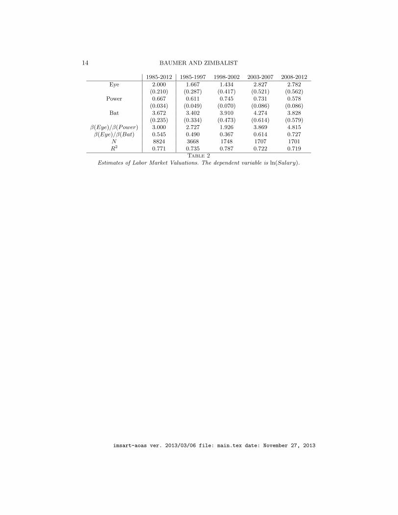
where Year is a vector of indicator variables for each year from 1986-2012,and γγγ is a vector of the corresponding coefficients. The results from thisregression are shown in Table 2. As we are using the same model as Hakes& Sauer, we attribute our slightly higher R2 values to the more accuratecontract data that we are using.

¡¡INSERT TABLE 2 HERE¿¿Here, unlike our estimates of labor market productivity, we see dramatic

changes in the way that players are compensated for certain skills on thelabor market over time. In particular, we note that whereas a free agentoutfielder of average ability in 2000 would expect to earn approximately$36,000 more had his walk rate been ten points higher, a player with thesame statistics could have expected approximately $125,000 in additionalsalary in 2010, more than a threefold increase.6 In Figure 2, we illustratethe changes in the coefficients for Eye,Bat, and Power over time.

¡¡INSERT FIGURE 2 HERE¿¿There appears to be greater fluctuation in the labor market valuations,

as opposed to the labor market productivity, but the evidence in favor ofstructural shifts is weak.7 As Hakes & Sauer noted that after reaching arelatively low point in 2001, the return to Eye begins to pick up in 2002 and

6Over the 1998-2002 period, the average values for TPA,Eye,Bat, and Power amongthe 1,748 players the data set were 447, 0.091, 0.272, and 1.59, respectively. If such a playerwere a free agent outfielder, then his 2000 salary predicted by our model is $2,424,780.However, if that players walk rate was 0.101, then his predicted salary becomes $2,460,973,an increase of $36,193. The corresponding difference for a free agent outfielder in 2010 withthe same statistics would be $124,655. Since we are using year fixed effects, this resultcontrols for baseball inflation over the period.

7The p-values for the F-statistic of the simple linear model for Eye,Bat, or Power asa function of Y ear are 0.089, 0.098, and 0.062. The corresponding p-values for a nestedF-test that includes in periodized interaction terms are 0.27, 0.846, 0.007. In particular,there is evidence that Power was compensated more highly from 1998-2007 than in theother years.



2003, prior to the publication of Moneyball . The return then spikes in 2004,the year following the book’s publication. They interpret these changes asevidence that Moneyball changed the labor market in baseball. In the longer-run context of the baseball labor market, while the rapid increase in the valueof Eye surrounding the publication of Moneyball may or may not be causal,a more robust story is that the assimilation of the value of OBP by generalmanagers has been a gradual change that has evolved over decades. Duringthe 28-year window explored, the post-Moneyball spike in the valuation ofEye is just a blip in a long-term change.8

In their 2007 paper, Hakes & Sauer question whether the noted decline inthe value of Eye from 2004 to 2006 is attributable to random variation, orevidence of a market correction among general managers who had come tosee Eye as being overvalued by the market. Although the valuation of Eyewas equally high in 2010, it does appear that the post-Moneyball valuationof Eye was abnormally high. Thus, while we see some evidence that theaverage valuation of Eye is higher in the post-Moneyball era, the immediateeffect of the book’s publication has been mitigated. Given the rigidities inthe baseball players’ market and the pile-on nature of market response, it isnot surprising that the observed annual market correction process is neithergradual nor linear.

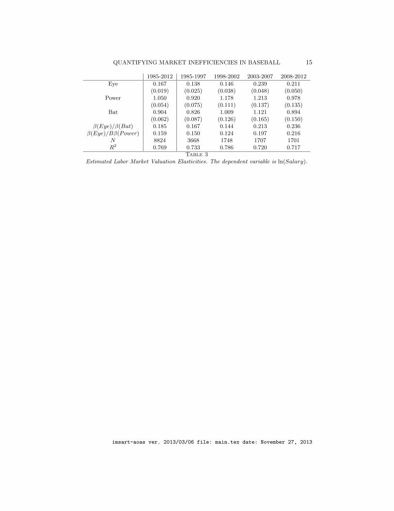
5. Elasticity Models. Since the three offensive performance variableshave different scales, it is desirable to consider the elasticity of salary withrespect to Eye,Bat, and Power, by taking logs on both sides of the regres-sion model. This represents a departure from Hakes and Sauer, and allowsus to interpret the coefficients as the percentage change in salary that isassociated with a 1% increase in each of the explanatory variables. In Table3, we provide results from this regression. We note that the salary returnto Eye increased by 5.8 percent (from 0.138 to 0.146) between the 1985-97and the 1998-2002 periods, but then shot up by 63.7 percent (from 0.146to 0.239) in the immediate post-Moneyball period, before retreating 11.7percent (from 0.239 to 0.211) during 2008-2012. It is also notable that thereturns to Power and Bat increased over the extended period as well9, al-though they did not grow as rapidly as the return to Eye. This result isevident in the Eye-to-Bat and Eye-to-Power coefficient ratios.

¡¡INSERT TABLE 3 HERE¿¿Similarly, we can consider our labor market productivity model in terms

8This point is elaborated in Baumer and Zimbalist (2014), chapter one.9This growth in the return to all skills should not be surprising given the sustained

increase in average salaries between 1985 ($370,000) and 2012 ($3.2 million).



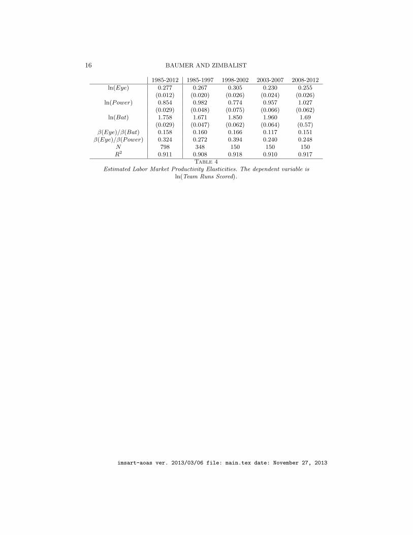
of elasticities. Since we include only salaries for position players in our labormarket valuation, here we include only offense, and use team runs scoredas the dependent variable. The results are shown in Table 4. We note thatthese coefficients show considerable long-term stability, with little evidenceof meaningful change over an extended period of time. This corroborates ourearlier observation that the elements of the game that translate into winningare relatively static.

¡¡INSERT TABLE 4 HERE¿¿By considering the ratio of the elasticity of each statistic to salary over

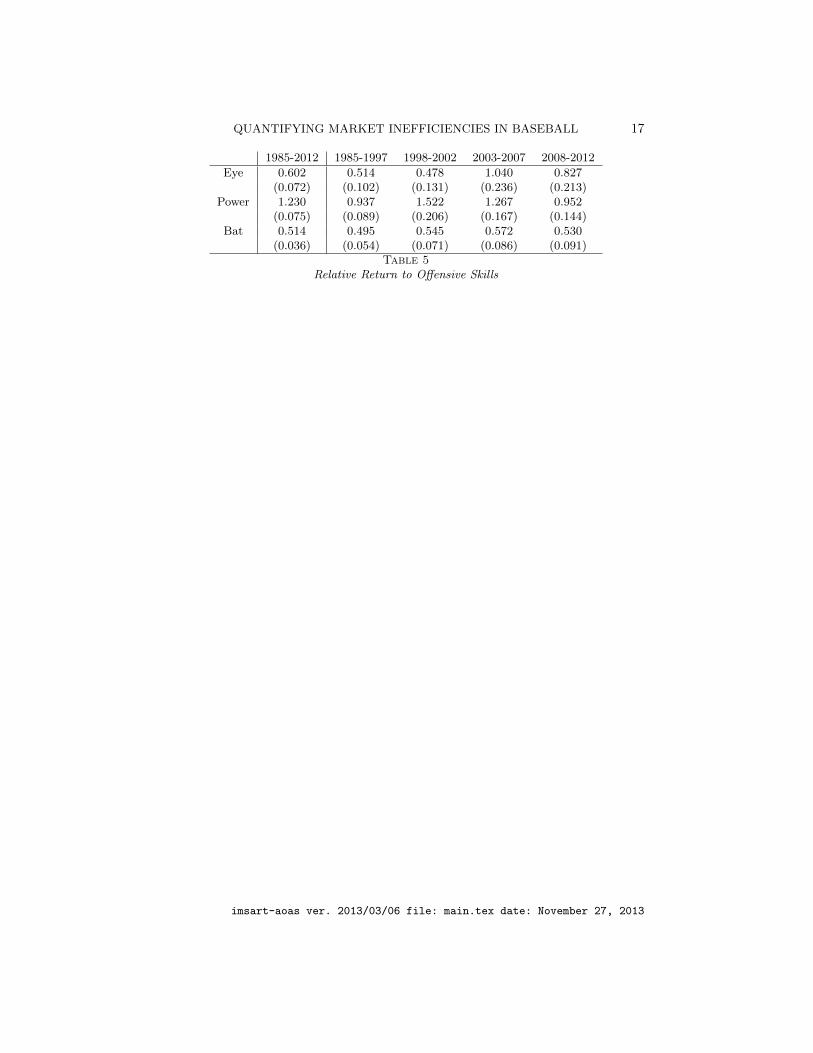
the elasticity of that statistic to runs scored, we gain an estimate of therelative return to each skill. We show these results in Table 5.

¡¡INSERT TABLE 5 HERE¿¿It is interesting to note here that the ratio of these elasticities for batting

average has remained remarkably consistent over these time periods. Thissuggests that however fairly batting average is being compensated on the la-bor market, that relationship has not changed much, if at all. Conversely, thereturn to Power has changed dramatically from sub-period to sub-period.It appears to now be only about half as high as it was during the home runboom of 1998-2002. However, it is also notable that between the 1985-1997and 2008-2012 periods the return to power has stayed relatively constant,increasing by only 1.6 percent. Conversely, the return to Eye increased by 61percent between the first and last periods. Moreover, the relative return toPower was three times higher than it was for Eye in the pre-Moneyball era,but in the most recent period is only slightly higher.10 Further, the patternof the relative return to Eye corresponds to the market correction processdescribed earlier. Namely, the relative return to Eye increases in the late1990s and the first three years of the 2000s, prior to the publication of Mon-eyball , accelerates sharply during 2003-2007 to the point of overcorrection,and then adjusts by falling 20 percent during 2008-2012.

6. Payroll Efficiency. Next we consider the relationship between teamwinning percentage and payroll, indexed as the share of league payroll.11

Hakes and Sauer posit that with the improved metrics of the Moneyball era,teams are better able to discern the true productivity of the players and,therefore, the statistical relationship between team payroll and performance

10It is also interesting to observe that the return to power was highest during the apexof the steroid power boom. While an economist might scratch her head at this outcome(thinking that the plethora of home runs would lower the relative value of the same), itappears that the steroid power boom produced both an ownership and fan fascinationwith the long ball, only serving to increase its market value.

11Equivalently, each teams payroll divided by the league average payroll in that season.



should tighten.Indeed, Hakes and Sauer found “the explanatory power of team payroll in

predicting winning percentage has improved over time,” citing as evidencethe increase in R2 values for a simple linear regression model for team win-ning percentage as a function of team payroll. Specifically, they found theR2 in this payroll model for all 587 team-seasons between 1986 and 2006to be 0.146. As noted above, the salary figures in the Lahman databaseare incomplete. Further, to derive team payroll data from individual playersalaries would require knowledge of the entire 25-man roster, the players onthe disabled and the proportion of a year that traded players were on theteam.

We use official payroll data from the Labor Relations Department of Ma-jor League Baseball, and find that the correct R2 over this time period is0.228, a substantial increase over the figure reported by Hakes and Sauer.In Table 6, we present the results from applying a regression model to teamwinning percentage as a function of each team’s LRD payroll.12

¡¡INSERT TABLE 6 HERE¿¿More importantly, Hakes and Sauer cited an increase in the strength of

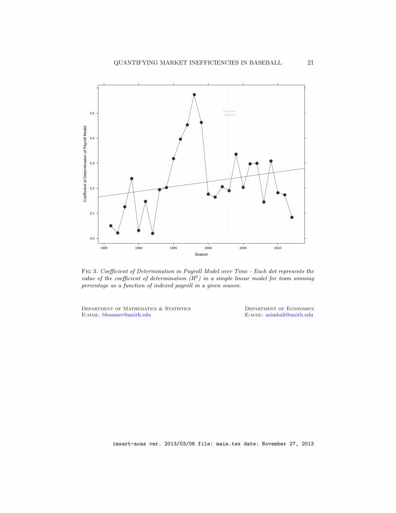
the relationship between team winning percentage and payroll over time asevidence that the window for exploiting market inefficiency in the mannerdescribed in Moneyball may be narrowing; or, stated differently, Hakes andSauer suggest that the new, improved performance metrics and correction ofmarket inefficiencies since Moneyball has tightened the relationship betweenteam payroll and win percentage. We find no such evidence. While it is truethat the predictive power of payroll upon winning percentage is higher thanit was in the 1980s and early 1990s, it has been much lower in the 2000s thanit was in the late 1990s, and shows few signs of a long-term upward trend (seeFigure 3).13 An elegant way to test for structural breaks in this relationship isto model winning percentage as a function of normalized payroll, along withinteraction terms for normalized payroll and an indicator variable for eachone of the periods. None of the terms involving any period was statisticallysignificant.

¡¡INSERT FIGURE 3 HERE¿¿

12LRD payroll stands for MLB’s Labor Relations Department measurement of payroll.LRD payroll differs from the CBT (competitive balance tax) and players’ associationpayroll in its treatment of benefits, deferred salary and discount rates.

13Again, a simple linear model for R2 in the payroll model as a function of time is notstatistically significant at the 5% level. The increase in R2 between 1985-1997 and 1998-2002 may be a function of widening revenue inequality across teams and the Yankees’remarkable string of success during the latter period.



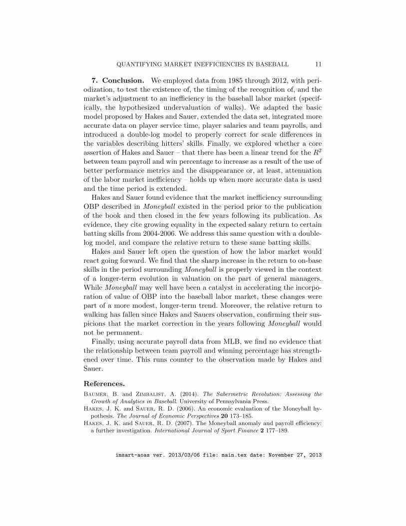
7. Conclusion. We employed data from 1985 through 2012, with peri-odization, to test the existence of, the timing of the recognition of, and themarket’s adjustment to an inefficiency in the baseball labor market (specif-ically, the hypothesized undervaluation of walks). We adapted the basicmodel proposed by Hakes and Sauer, extended the data set, integrated moreaccurate data on player service time, player salaries and team payrolls, andintroduced a double-log model to properly correct for scale differences inthe variables describing hitters’ skills. Finally, we explored whether a coreassertion of Hakes and Sauer – that there has been a linear trend for the R2

between team payroll and win percentage to increase as a result of the use ofbetter performance metrics and the disappearance or, at least, attenuationof the labor market inefficiency – holds up when more accurate data is usedand the time period is extended.

Hakes and Sauer found evidence that the market inefficiency surroundingOBP described in Moneyball existed in the period prior to the publicationof the book and then closed in the few years following its publication. Asevidence, they cite growing equality in the expected salary return to certainbatting skills from 2004-2006. We address this same question with a double-log model, and compare the relative return to these same batting skills.

Hakes and Sauer left open the question of how the labor market wouldreact going forward. We find that the sharp increase in the return to on-baseskills in the period surrounding Moneyball is properly viewed in the contextof a longer-term evolution in valuation on the part of general managers.While Moneyball may well have been a catalyst in accelerating the incorpo-ration of value of OBP into the baseball labor market, these changes werepart of a more modest, longer-term trend. Moreover, the relative return towalking has fallen since Hakes and Sauers observation, confirming their sus-picions that the market correction in the years following Moneyball wouldnot be permanent.

Finally, using accurate payroll data from MLB, we find no evidence thatthe relationship between team payroll and winning percentage has strength-ened over time. This runs counter to the observation made by Hakes andSauer.

References.

Baumer, B. and Zimbalist, A. (2014). The Sabermetric Revolution: Assessing theGrowth of Analytics in Baseball. University of Pennsylvania Press.

Hakes, J. K. and Sauer, R. D. (2006). An economic evaluation of the Moneyball hy-pothesis. The Journal of Economic Perspectives 20 173–185.

Hakes, J. K. and Sauer, R. D. (2007). The Moneyball anomaly and payroll efficiency:a further investigation. International Journal of Sport Finance 2 177–189.



Lahman, S. (2013). Sean Lahman’s Baseball Database. http://www.seanlahman.com/

baseball-archive/statistics/.Lewis, M. (2003). Moneyball: The Art of Winning an Unfair Game. WW Norton &

Company.Sarkar, D. (2008). Lattice: Multivariate Data Visualization with R. Springer, New York.R Core Team (2012). R: A Language and Environment for Statistical Computing R

Foundation for Statistical Computing, Vienna, Austria.


http://www.seanlahman.com/baseball-archive/statistics/

http://www.seanlahman.com/baseball-archive/statistics/


1985-2012 1985-1997 1998-2002 2003-2007 2008-2012

Constant 0.500 0.500 0.500 0.500 0.500Eye 1.713 1.862 1.555 1.758 1.419

(0.081) (0.136) (0.167) (0.157) (0.217)Power 0.264 0.272 0.219 0.260 0.319

(0.016) (0.027) (0.031) (0.034) (0.039)Bat 3.005 2.907 3.266 2.911 3.087

(0.074) (0.119) (0.150) (0.162) (0.174)β(Eye)/β(Bat) 0.570 0.641 0.476 0.604 0.460β(Eye)/β(Power) 6.497 6.839 7.117 6.747 4.448

N 798 348 150 150 150R2 0.814 0.773 0.882 0.827 0.808

Table 1Estimates of Labor Market Productivity. The dependent variable is Team Winning

Percentage. Note: In all tables, standard errors are in parentheses below the coefficients.



1985-2012 1985-1997 1998-2002 2003-2007 2008-2012

Eye 2.000 1.667 1.434 2.827 2.782(0.210) (0.287) (0.417) (0.521) (0.562)

Power 0.667 0.611 0.745 0.731 0.578(0.034) (0.049) (0.070) (0.086) (0.086)

Bat 3.672 3.402 3.910 4.274 3.828(0.235) (0.334) (0.473) (0.614) (0.579)

β(Eye)/β(Power) 3.000 2.727 1.926 3.869 4.815β(Eye)/β(Bat) 0.545 0.490 0.367 0.614 0.727

N 8824 3668 1748 1707 1701R2 0.771 0.735 0.787 0.722 0.719

Table 2Estimates of Labor Market Valuations. The dependent variable is ln(Salary).



1985-2012 1985-1997 1998-2002 2003-2007 2008-2012

Eye 0.167 0.138 0.146 0.239 0.211(0.019) (0.025) (0.038) (0.048) (0.050)

Power 1.050 0.920 1.178 1.213 0.978(0.054) (0.075) (0.111) (0.137) (0.135)

Bat 0.904 0.826 1.009 1.121 0.894(0.062) (0.087) (0.126) (0.165) (0.150)

β(Eye)/β(Bat) 0.185 0.167 0.144 0.213 0.236β(Eye)/Bβ(Power) 0.159 0.150 0.124 0.197 0.216

N 8824 3668 1748 1707 1701R2 0.769 0.733 0.786 0.720 0.717

Table 3Estimated Labor Market Valuation Elasticities. The dependent variable is ln(Salary).



1985-2012 1985-1997 1998-2002 2003-2007 2008-2012

ln(Eye) 0.277 0.267 0.305 0.230 0.255(0.012) (0.020) (0.026) (0.024) (0.026)

ln(Power) 0.854 0.982 0.774 0.957 1.027(0.029) (0.048) (0.075) (0.066) (0.062)

ln(Bat) 1.758 1.671 1.850 1.960 1.69(0.029) (0.047) (0.062) (0.064) (0.57)

β(Eye)/β(Bat) 0.158 0.160 0.166 0.117 0.151β(Eye)/β(Power) 0.324 0.272 0.394 0.240 0.248

N 798 348 150 150 150R2 0.911 0.908 0.918 0.910 0.917

Table 4Estimated Labor Market Productivity Elasticities. The dependent variable is

ln(Team Runs Scored).



1985-2012 1985-1997 1998-2002 2003-2007 2008-2012

Eye 0.602 0.514 0.478 1.040 0.827(0.072) (0.102) (0.131) (0.236) (0.213)

Power 1.230 0.937 1.522 1.267 0.952(0.075) (0.089) (0.206) (0.167) (0.144)

Bat 0.514 0.495 0.545 0.572 0.530(0.036) (0.054) (0.071) (0.086) (0.091)

Table 5Relative Return to Offensive Skills



1985-2012 1985-1997 1998-2002 2003-2007 2008-2012

Payroll 0.089 0.090 0.107 0.085 0.074(0.006) (0.011) (0.013) (0.012) (0.013)

N 798 348 150 150 150R2 0.214 0.166 0.304 0.257 0.171

Table 6Payroll Efficiency. The dependent variable is Team Winning Percentage.



Estimated Productivity Coefficients

Season

Net

Cha

nge

in W

inni

ng P

erce

ntag

e

0

1

2

3

4

1985 1990 1995 2000 2005 2010

Moneyball

Published

Eye Bat Power

Fig 1. Estimated Labor Market Productivity Coefficients



Estimated Labor Market Valuation Coefficients

Season

Log

of S

alar

y (U

SD

)

0

2

4

6

1985 1990 1995 2000 2005 2010

Moneyball

Published

Eye Bat Power

Fig 2. Estimated Labor Market Valuation Coefficients



Season

Coe

ffici

ent o

f Det

erm

inat

ion

of P

ayro

ll M

odel

0.0

0.1

0.2

0.3

0.4

0.5

1985 1990 1995 2000 2005 2010

Moneyball

Published

Fig 3. Coefficient of Determination in Payroll Model over Time - Each dot represents thevalue of the coefficient of determination (R2) in a simple linear model for team winningpercentage as a function of indexed payroll in a given season.

Department of Mathematics & StatisticsE-mail: [email protected]

Department of EconomicsE-mail: [email protected]


mailto:[email protected]

mailto:[email protected]

quantifying market inefficiencies in the baseball players...

Documents