Quantifying Multistate Cytoplasmic Molecular Diffusion in BacterialCells via Inverse Transform of Confined Displacement DistributionTai-Yen Chen,† Won Jung,† Ace George Santiago, Feng Yang, Łukasz Krzeminski, and Peng Chen*

Department of Chemistry and Chemical Biology, Cornell University, Ithaca, New York 14853, United States

*S Supporting Information

ABSTRACT: Single-molecule tracking (SMT) of fluorescentlytagged cytoplasmic proteins can provide valuable information onthe underlying biological processes in living cells via subsequentanalysis of the displacement distributions; however, the confine-ment effect originated from the small size of a bacterial cell skewsthe protein’s displacement distribution and complicates thequantification of the intrinsic diffusive behaviors. Using theinverse transformation method, we convert the skewed displace-ment distribution (for both 2D and 3D imaging conditions) backto that in free space for systems containing one or multiple(non)interconverting Brownian diffusion states, from which wecan reliably extract the number of diffusion states as well as theirintrinsic diffusion coefficients and respective fractional populations. We further demonstrate a successful application toexperimental SMT data of a transcription factor in living E. coli cells. This work allows a direct quantitative connection betweencytoplasmic SMT data with diffusion theory for analyzing molecular diffusive behavior in live bacteria.

1. INTRODUCTION

Diffusive behaviors of membrane and cytoplasmic molecules incells carry valuable information on the underlying biologicalprocesses, such as membrane protein oligomerization,1

protein−membrane interactions,2 protein−DNA interactions,3

DNA repair,4 cytokinesis,5 and chromosome diffusion.6 Becausethese processes fulfill many cellular functions, quantifying thediffusive behaviors of these molecules is important forunderstanding the underlying mechanisms.A number of techniques have been developed to study the

diffusive behaviors of membrane and cytoplasmic molecules.Fluorescence recovery after photobleaching (FRAP),7 fluo-rescence correlation spectroscopy (FCS),8 and single-moleculetracking (SMT)9 are the three most common fluorescence-based methods.10 Both FRAP and FCS probe moleculardiffusive behaviors within a small volume defined by the laserfocus; however, the slow time resolution and potential DNAdamage caused by photobleaching in FRAP,11 the susceptibilityto optical aberrations in FCS,12 and the diffraction-limitedspatial resolution constrain the application of FRAP and FCS tomolecular diffusions in live cells. On the other hand, recenttechnological advances in camera, fluorescent protein (FP)reporters, and super-resolution imaging algorithm13 made itpossible to track individual molecules with high spatial (fewnanometers) and temporal (microseconds) resolution14 in livecells.15 Imaging one molecule at a time typically is throughimaging a fluorescent tag, which is often a regular orphotoconvertible FP. Even though the photobleaching of thefluorescent tag limits the observation time, recent studies haveshown that SMT is particularly powerful in dissecting the

mechanisms of biophysical processes.16,17 Using probes such asquantum dots or plasmonic nanoparticles can further extendSMT trajectories in time.18

Through real-time SMT, one directly obtains the diffusivebehavior of each fluorescently labeled protein molecule in thecell reflected by its location versus time trajectory. Quantitativemethods to analyze the SMT trajectories include mean-squareddisplacement (MSD), hidden Markov modeling (HMM),19−22

and probability distribution function (PDF) or cumulativedistribution function (CDF) of displacement length analyses.MSD analysis, the most popular method, reliably determinesthe diffusion coefficient for molecules moving in free space witha single diffusion state.23 For molecules having transientdiffusive behaviors or those containing multiple diffusion states,MSD method is less ideal due to its requirement of averagingover all displacements.24 HMM analysis, a probabilisticmaximum-likelihood algorithm, can extract the number ofdiffusion states and their interconversion rate constants (withcertain assumptions);21,22,25 it provides a mathematicallyderived routine and unbiasedly analyses SMT trajectories, butthe resulting multistate diffusion model often lacks a definitivenumber of states.26 The HMM analysis of SMT trajectories isfurther constrained by the complex computational algorithmand the difficulty in incorporating the photophysical kinetics ofthe fluorescent probe. Analysis of the PDF or CDF ofdisplacement length on the basis of Brownian diffusion model

Received: September 4, 2015Revised: October 7, 2015Published: October 22, 2015

Article

pubs.acs.org/JPCB

© 2015 American Chemical Society 14451 DOI: 10.1021/acs.jpcb.5b08654J. Phys. Chem. B 2015, 119, 14451−14459

is known to be a robust way to quantify the diffusioncoefficients and fractional populations of multistate systems, asdemonstrated both in vitro and in vivo,3−5,27−29 even though itrequires more control experiments and elaborate analysis basedon a defined kinetic model to extract the minimal number ofdiffusion states and their interconversion rate constants.One factor that significantly affects the PDF or CDF analysis

of cytoplasmic diffusion displacement is the confinement by thecell volume, especially for bacterial cells, which are less than afew microns in size. This confinement distorts and compressesthe displacement length distribution, especially for moleculeswith large diffusion coefficients. SMT trajectories obtained fromcells with different geometries can give significantly biaseddisplacement length distributions, even though the underlyingdiffusion coefficient is the same. As a result, fitting thedistribution of displacement length with PDF or CDF derivedfrom the Brownian diffusion model (or any other model) onlyreports apparent diffusion coefficients, which are typicallysmaller than the intrinsic diffusion coefficients.For membrane protein diffusion, it is a two dimension (2D)

diffusion on a surface curved in three dimension (3D) space,and it does not actually have boundary confinement, as the cellmembrane is a continuous boundary-less surface; however,SMT trajectories are generally obtained in 2D, where only thex, y movements in the imaging plane are tracked, thusprojecting the boundary-less movements of membrane proteindiffusion into a 2D diffusion confined by the cell boundary.This confinement effect from 2D projection of membranediffusion distorts and compresses the displacement lengthdistribution as well. To address this projection-inducedconfinement effect, Peterman and coworkers introduced theinverse projection of displacement distribution (IPODD)method30 in analyzing simulated one-state membrane diffusionin bacterial cells (e.g., E. coli). In short, they first created aprojected displacement distribution (PDD) matrix for a givencell geometry by projecting the simulated membrane displace-ment vectors onto the 2D imaging plane. For each displacementlength that could occur anywhere on the membrane surface,they determined the resulting distribution of displacementlength after projection. The PDD matrix thus quantifies therelationship from the displacement distribution before projec-tion to that after projection. Using inverse transformation, theycould then convert the 2D-projected displacement lengthdistribution (which is often the one determined experimen-tally) into a most probable displacement length distribution onthe cell membrane, which is readily analyzed to give theintrinsic diffusion coefficient.Here we report an extension of the inverse transformation

method for membrane diffusion to analyze cytoplasmicmolecular diffusions. Using simulated diffusion trajectories infree and confined spaces, we demonstrate this inversetransformation method in analyzing 1-state cytoplasmicBrownian diffusions in both 2D and 3D and with varyingdiffusion coefficients and cell geometries. We further extendthis method to multistate cytoplasmic diffusions, containingnoninterconverting or interconverting states, to effectivelyextract the minimal number of diffusion states as well as theirrespective diffusion coefficients and fractional populations.Finally, we demonstrate a successful application to experimentalSMT data of a transcription factor in living E. coli cells, whichshows interconverting multistate diffusive behaviors.

2. METHODS

2.1. Simulations of Single-Molecule Diffusion Trajec-tories. On the basis of the Brownian diffusion model, we usedhome-written Matlab codes to simulate 3D single-moleculediffusion trajectories that contained one, three noninterconvert-ing, or three interconverting diffusion states in both free spaceand confined space. Each simulation condition contained atleast 100 000 diffusion trajectories to ensure statisticallysaturated data for analysis. The 2D diffusion trajectories weregenerated from the 3D ones by discarding the z-component.

Diffusion Trajectories in Free Space. The 3D diffusiontrajectories in free space containing one diffusion state weresimulated via the following steps. First, we randomly sampledthe initial position (x, y, z) in free space, where the values of x,y, and z are each from a randomly generated number. Second,with the input diffusion coefficient D we generated thedistribution of displacement vector ( ri, where i = x, y, or z)following Brownian diffusion in free space as described by eq 1,where n = 1, for each of the three dimensions (i.e., x, y, and z)and using a time resolution t = 4 or 60 ms. Third, we randomlychose a ri from the distribution of the displacement vector,together with the initial position, to calculate the subsequentposition, which also served as the new initial position for thenext simulation step. The procedure was then repeated until thelength of the final moving trajectory contained 10 positions foranalysis. Trajectories for three noninterconverting states weregenerated as that in single diffusion state case but with D of0.036, 0.7, and 11 μm2 s−1, separately.The 3D diffusion trajectories that contained three

interconverting diffusion states were simulated with threeinput diffusion coefficients Di (i = 1, 2, or 3) and theirassociated interconversion rate constants (e.g., rate constant γijfor interconversion from state i to j; i ≠ j and i, j = 1, 2, or 3). Asequence of residence time on the diffusion state i was built,where each residence time ti sampled the residence timedistribution exp(−∑jγijt), where Σj was a sum of all competingprocesses leaving from state i to state j (j ≠ i), each with a rateconstant γij. The transition from state i to a particular state jfollowed the relative probability (γij/∑jγij). The residence timesequence was terminated by tbl, which equaled the sum of allresidence times in the sequence, and tbl samples the distributionexp(−kbl(Tint/Ttl)t), which was limited by the photobleachingand photoblinking of the fluorescence tag, where kbl is the tag’sintrinsic photobleaching and photoblinking rate constant. Tintand Ttl are the laser exposure time and stroboscopic imaginglapse time, respectively. During each state, the generation ofdisplacements was the same as described in the one diffusionstate case. Here we first generate the primary diffusiontrajectories with Tint and Ttl of 4 ms. For trajectories withlonger Ttl, the primary diffusion trajectories were resimulatedand sampled at every lapse time Ttl to give the eventualsimulated diffusion trajectory, which is analyzed.

Diffusion Trajectories in Confined Space. To mimic the 3DSMT data in a bacterium cell, we first modeled the 3D cellgeometry as a cylinder capped by two hemispheres forsimplicity with cell length and width adapted from ourexperimental results. The 3D diffusion trajectories in a confinedspace (i.e., the cell volume) were generated by similarprocedures as described in free space but with randomselection of initial positions inside the cell volume and theimplementation of confinement effect with the boundaryreflection from the cell surface. Boundary reflection was

The Journal of Physical Chemistry B Article

DOI: 10.1021/acs.jpcb.5b08654J. Phys. Chem. B 2015, 119, 14451−14459

14452

performed when the end point of displacement vector isoutside the cell volume. The intercept of cell boundary anddisplacement vector, together with the normal plane, wascalculated for subsequent evaluation of the reflected position.The corresponding 2D simulated data were then generatedfrom 3D ones by discarding the diffusion information in the zdirection. The 3D diffusion trajectories for systems with threeinterconverting diffusion states in confined space weresimulated in the same way as in free space but with appliedboundary reflection in the displacement generation step.2.2. Generation of Confinement Transformation

Matrix. Generation of the confinement transformation matrix([CTM]) was inspired by Peterman’s work on inverseprojection of displacement distributions (IPODD) for analyz-ing membrane proteins diffusing on the curved surface. Inshort, >100 000 displacement vectors (r) of a given distancelength r were randomly positioned in the cell. If the end pointof displacement vector was outside the cell volume, the

boundary reflection was performed, generating final positions.We then calculated the output r from the final positions andcreated the confined displacement distribution (CDD), whichserved as a single column data for the [CTM]. The length ofdisplacement vector varied from 10 nm to 2.82 μm (i.e., up tothe cell length) with 10 and 30 nm increments for transformingsimulated and experimental data, respectively. Finally, CDDsfor all input displacement vectors were combined to form theconfinement transformation matrix.

2.3. Generation of Probability Density Function ofDisplacement Length for Systems with Multi DiffusionStates. All probability density functions (PDFs) of displace-ment length (PDF(r)) in this study were generated from thedistribution of displacement length of moving trajectoriesnormalized by the area of distribution. For example, for systemswith a single diffusion state, displacements were calculated fromthe moving trajectory and used to generate the histogram ofdisplacement length for a given bin size (i.e., 10 and 30 nm for

Figure 1. Illustration of inverse transform of confined displacement distribution (ITCDD) using simulated Brownian diffusions. (A) Schematicoverview of ITCDD. Single-molecule diffusion trajectories are first generated in 3D in free or confined space (black trajectories) with t = 60 ms.Removing the z component from 3D trajectories results in the corresponding projected 2D trajectories (red trajectories). Converting thedisplacement length distribution in confined space to that in free space is achieved via inverse transformation of confined displacement distributionusing the confinement transformation matrix ([CTM]). Here all confined diffusion simulations were performed within a cell having width (W) andlength (L) of 1.15 and 2.82 μm, respectively. (B) [CTM] for the 3D output displacements in confined space given 3D input displacements in freespace. The input r is from 10 to 2820 nm with 10 nm increment. (C) CDD from B at 3D input displacement with length of 2.5 μm. (D) Overlay ofsimulated displacement length distributions in 3D free space (PDFFS, blue shade) and in confined space (PDFCS, green shade). Apply ITCCD onPDFCS recovers the displacement length distribution (red symbols) that agrees well with that in free space. Both the simulated PDFFS and ITCDDmatch the theoretical displacement length distribution (black line) of the Brownian diffusion model. All distributions are normalized with theintegrated area being one. (E,F), same as panels B and D but for 2D case. (G, H) Same as panels B and D but the [CTM] is from 3D inputdisplacement to 2D output displacement. ITCDD (red dots) clearly deviates from the theoretical displacement length distribution from theBrownian diffusion model (black line).

The Journal of Physical Chemistry B Article

DOI: 10.1021/acs.jpcb.5b08654J. Phys. Chem. B 2015, 119, 14451−14459

14453

simulated and experimental data, respectively). The displace-ment histogram was then divided by its area to create the PDFof displacement length, PDF(r).PDF(r) for systems with static three diffusion states was

obtained as follows. We combined displacements from therespective diffusion states with given weighting coefficients togenerate the displacement length histogram, which was thennormalized by its area to create the PDF(r) for analysis. Forexample, after simulating 100 000 trajectories (with trajectorylength of 10 positions) in a given cell geometry for each ofthree different Dinput, we randomly chose trajectories from eachdiffusion state and combined them with chosen fractionalpopulations for subsequent analyses.Finally, for system with three interconverting diffusion states,

the PDF(r) was generated from moving trajectories based onprocedures as described in the Methods section. Because themoving trajectories were simulated with three interconvertingdiffusion states built-in, the PDF(r) was simply the resultingdisplacement histogram normalized by the histogram area.2.4. Transformation of Distribution of Displacement

Length between Free and Confined Spaces. Trans-formation of distribution of displacement length between freeand confined spaces was achieved via the confinementtransformation matrix ([CTM]). Forward converting the 2Dor 3D distribution of displacement length in free space to thatin confined space was via direct multiplication of the 2D or 3Ddistribution in free space with [CTM]. As for the inversetransformation (i.e., distribution in confined space to that infree space) process, the inverted [CTM] (i.e., [CTM]−1) wasfirst obtained using Gaussian elimination; multiplication of thedistribution of displacement length in confined space with the[CTM]−1 (i.e., eq 4) then resulted in the correspondingdistribution in free space. Note that in the [CTM]−1 obtainingstep we first diagonalized the [CTM] and back-substituted theknown variables to solve for [CTM]−1 rather than simplytranspose the [CTM].

3. RESULTS AND DISCUSSIONS

3.1. Inverse Transform of Confined DisplacementDistribution for Cytoplasmic Molecules. The diffusivemotions of cytoplasmic molecules in a bacterial cell aresignificantly confined by the small cell size (Figure 1A, right) (atypical E. coli cell is about 0.5 × 0.5 × 2 μm3 in size (e.g., ∼ 1.5fL)), and for a small protein with a diffusion coefficient of 10μm2 s−1, its diffusion can traverse the cell length in ∼100 ms.This confinement effect distorts the molecule’s displacementdistribution, hindering the quantification of its diffusioncoefficient. For heterogeneous diffusion where multiplediffusion states are present, this confinement effect also hindersthe determination of the (minimal) number of diffusion states.Here we present an inverse transform method to analyzedisplacement distributions of confined diffusions to obtaindisplacement distributions that are well-described by Browniandiffusion in free space. The feasibility of the method isexamined by diffusion simulations in free and confined spaces.For 3D Brownian diffusion in free space, the probability

density distribution of displacement vector r within time tfollows a Gaussian function

π = − ⎛

⎝⎜⎞⎠⎟

⎛⎝⎜

⎞⎠⎟P r t

DtrDt

( , )1

4exp

4

n 2

(1)

where D is the diffusion coefficient and n = 1, 2, or 3 for 1D,2D, or 3D diffusion, respectively. The second moment of r follows the well-known relationship ⟨r 2⟩ = 2nDt. The PDF ofthe 3D and 2D displacement length, r, which is the scalarcomponent of r, can be obtained by integrating P(r, t) over allangular spaces

π= −

⎛⎝⎜

⎞⎠⎟r t

rDt

rDt

PDF( , )4 ( )

exp4

, (3D)2

3/2

2

(2)

= −⎛⎝⎜

⎞⎠⎟r t

rDt

rDt

PDF( , )2

exp4

, (2D)2

(3)

The blue shade in Figure 1D shows the distribution ofdisplacement length r from a simulation of 3D Browniandiffusion in free space with D = 1 μm2 s−1 and t = 60 ms(simulation details in the Methods section), which is well-described by eq 2 (Supplementary Figure S1). As most of theSMT experiments are done in 2D imaging mode, the blueshade in Figure 1F presents the distribution of thecorresponding displacement length r in 2D, which is againwell-described by eq 3) (Supplementary Figure S1). When thesame Brownian diffusion is simulated inside a confined space(e.g., inside a bacterial cell, Figure 1A, right), the distributionsof displacement length r in both 3D and 2D are significantlydistorted due to reflections by cell boundaries (Figure 1D,F), asexpected. These confined displacement length distributions donot follow eqs 2 and 3, and attempted fitting gives the diffusionconstant of 0.76 ± 0.32 μm2 s−1, underestimated from theexpected diffusion coefficient of 1 μm2 s−1.To numerically mimic the confinement effect on the

displacement length distribution, we followed Peterman etal.30 to generate a confinement transformation matrix ([CTM];e.g., Figure 1B) for a given cell geometry, which is readilymeasured for bacterial cells. For each column of this matrix, a3D displacement vector in free space of a given length israndomly sampled within the cell volume and applied boundaryreflections when the vector impinges on the cell boundary. Inthis way, it generates a distribution of corresponding 3Ddisplacement in the confined space. Normalizing thisdistribution gives the CDD, which represents the probabilitydistribution for finding a 3D-confined displacement lengthgiven a 3D displacement of a particular length in free space(Figure 1C). Varying the length of the 3D displacement vectorin free space and repeating the random sampling processgenerates the data for all other columns in [CTM] (Figure 1B).The utility of this confinement transformation matrix can beseen by applying it to the distribution of displacement lengthfrom the simulated 3D Brownian diffusion in free space as[CTM]·PDFFS = PDFCS, where PDFFS and PDFCS are PDFs ofdisplacement length in free and confined spaces, respectively.The resulting distribution from this forward transformationreproduces that from the simulations in the confined space(Supplementary Figure S2A).More useful is the inverse transformation of the confined

displacement distribution (ITCDD), as the CDD is what isdirectly measured in experiments

= ·−PDF [CTM] PDFFS1

CS (4)

where [CTM]−1 can be obtained by Gaussian elimination(Section 2.4). Applying ITCDD on the simulated results in theconfined space deconvolutes the confinement effect andeffectively reproduces the theoretical distribution of displace-

The Journal of Physical Chemistry B Article

DOI: 10.1021/acs.jpcb.5b08654J. Phys. Chem. B 2015, 119, 14451−14459

14454

ment length r in free space (Figure 1D). Fitting the inversetransformed distribution gives D = 1.04 ± 0.01 μm2 s−1, reliablyrecovering the expected diffusion coefficient (D = 1 μm2 s−1).All fittings of the ITCDD were done via least-squares fitting inMATLAB program using PDFs with single or three diffusionstates (e.g., eqs 3 and 5, respectively, for the 2D diffusion cases)The forward transformation, and more importantly, the

inverse transformation using the confinement transformationmatrix are equally applicable between the 2D displacementlength distribution in free space and that in confined space(Figure 1E,F and Supplementary Figure S2B).It is important to point out that these forward and inverse

transformations only work well when the confinementtransformation matrix is generated when the input and outputdisplacements match in dimension. Figure 1G shows the[CTM] generated between 3D displacement in free space andthe 2D displacement in confined space. Using this [CTM] or[CTM]−1 for forward or inverse transformation cannotreproduce the expected distributions (Figure 1H andSupplementary Figure S2C). It is worth noting that the originalPeterman’s work on membrane diffusion is between 2Ddiffusion in curved surface and its 2D projection onto a flatsurface,30 where the displacement dimensions are matching. Alikely reason for the inapplicability of transformation betweendifferent dimensions is that the lower dimension displacementsare missing information about the third dimension; this misseddimension cannot be created during the transformation to thehigher dimension displacements.3.2. Analysis of One Diffusion State in Cells: Variation

in Diffusion Coefficient and Cell Geometry. The diffusioncoefficient (D) of cytosolic molecules in bacteria typicallyranges from 10−2 to 10 μm2 s−1.31 To probe whether themagnitude of the diffusion coefficient may affect the perform-ance of the inverse transformation method, we simulateddiffusion trajectories with variable D values. Because most ofSMT experiments are done in 2D, we focus discussions andanalyses on the 2D displacements generated from simulateddiffusions that are always done in 3D; the results apply equallyto the 3D displacements.Figure 2A shows the simulated 2D PDF(r) values in free

space and in a confined cell volume with the input D of 11 μm2

s−1, a typical diffusion coefficient for a fast-diffusing smallprotein in bacterial cytoplasm, for which the confinement effectis more significant than those with smaller diffusion coefficients.The corresponding ITCDD closely mimics that in free space(Figure 2A); fitting it with eq 3 gives Dfit of 12.5 ± 0.2 μm2 s−1,within 14% of the input D. With the input D varying from 0.01to 11 μm2 s−1, the fitted D from ITCDD is always within 0.1−14% of the input D (Figure 2B), smaller than or comparable totypical experimental uncertainties (8−25%).3,27 Therefore, theinverse transformation method allows for direct and reliableextraction of the intrinsic diffusion coefficients of Browniandiffusions in confined space.Using a fixed input D (e.g., 11 μm2 s−1), we further evaluated

how the cell geometry, which the [CTM] is dependent on,might affect the performance of the inverse transformationmethod. We examined Brownian diffusions in cells with widthof 1.15 μm and lengths of 2.32, 2.82, and 3.32 μm,corresponding to aspect ratios of 2.0, 2.5, and 2.9, respectively.These geometries cover the range of E. coli cell shapes typicallyobserved in minimum growth medium.3 Regardless of the cellgeometry, the fitted D from ITCDD stays at 12.4 ± 0.5 μm2

s−1, within 13% of the input D (Figure 2C). To further test the

insensitiveness of the inverse transformation method to cellgeometry within this range, we combined the simulateddistributions of displacement lengths from these three differentgeometries but applied merely the [CTM] from the cells oflength = 2.82 μm, which is about the average of the three celllengths; fitting the ITCDD with eq 3 again gives an Dfit of 12.3± 0.2 μm2 s−1, close to the input D. Therefore, even whendiffusion trajectories are collected from a population of cellsthat differ in geometry (within the range evaluated here), it issufficient to use the [CTM] for the average cell geometry toperform ITCDD to extract the intrinsic diffusion coefficient.

3.3. Analysis of Noninterconverting Multistate Dif-fusions in Cells. Inside a cell, a protein molecule may have afew different diffusive behaviors depending on its interactionswith other proteins, RNA, or DNA. We thus evaluated theinverse transformation method in analyzing diffusion trajecto-ries that contain multiple (i.e., three) Brownian diffusion states.We first examined the case that these states do not interconvert,that is, a static mixture of diffusive behaviors. We again focus onthe analysis of the 2D displacements here from 3D simulations.The diffusion coefficients (Dinput) of diffusion states were set to11 (D1), 0.7 (D2), and 0.036 (D3) μm

2 s−1, respectively, close tothose we previously measured for a transcription factor in E. colicells,3 and the fractional population (A3) of the D3 state wasvaried from 5 to 33% while the other two fractional populationswere set as A1 = A2 = (1 − A3)/2.Figure 3A shows the 2D PDF(r) from such a three-state

simulation in a cell volume. The corresponding ITCDD can befitted using a linear combination of PDF(r) (eq 5), eachaccounting for one diffusion state with its correspondingfractional population (A) as a weighting coefficient

Figure 2. Analysis of one diffusion state inside a cell with ITCDD. (A)Simulated PDF(r) data of diffusion trajectories in free (blue shade)and confined (green shade) spaces with Dinput of 11 μm

2 s−1 and t = 60ms. Multiplication of PDF(r) of diffusion trajectories in confined spacewith [CTM]−1 resulted in the corresponding ITCDD (red circles),which reproduces the theoretical distribution (black curve) based onthe Brownian model. (B) Fitted diffusion coefficients of ITCDD atvarious input diffusion coefficients. (C) Fitted diffusion coefficients ofITCDD (Dinput of 11 μm2 s−1) with cell lengths varying from 2.32 to2.82 μm. The fit result of the combined ITCCD with the average celllength of 2.82 μm is also plotted for comparison.

The Journal of Physical Chemistry B Article

DOI: 10.1021/acs.jpcb.5b08654J. Phys. Chem. B 2015, 119, 14451−14459

14455

= − + −

+− −

−

⎛⎝⎜

⎞⎠⎟

⎛⎝⎜

⎞⎠⎟

⎛⎝⎜

⎞⎠⎟

r tA rD t

rD t

A rD t

rD t

A A rD t

rD t

PDF ( , )2

exp4 2

exp4

(1 )2

exp4

3state1

1

2

1

2

2

2

2

1 2

3

2

3 (5)

The fitted D values of all three states are all within 10% error ofDinput (Figure 3B). The fitted fractional populations are also inagreement with input ones (within 7% error), showing a cleartrend of increasing A3 and decreasing A1 and A2, as expected.Therefore, the inverse transformation method can effectivelyextract the intrinsic diffusion coefficients and their fractionalpopulations of noninterconverting multistate diffusions.3.4. Analysis of Interconverting Multistate Diffusions

in Cells. Following the above section, we further evaluated theinverse transformation method in analyzing diffusion trajecto-ries that contain three interconverting Brownian diffusionstates. We simulated the 3D diffusion trajectories with 4 mstime resolution in a cell volume using a set of interconversionkinetic rate constants (Methods section) from our previousSMT study of the transcription factor CueR, which was taggedby a photoconvertible FP mEos3.2.32 Table 1 gives inputparameters of this simulation, including diffusion coefficients(Di, i = 1−3) and interconverting rate constants (γij; i, j = 1, 2,or 3); the interconversion rate constants also determine thefractional populations of the respective states. We furtherincluded a photobleaching rate constant (kbl) to account for thefact that FP’s photobleaching limits the length of trackingtrajectories. Note that no interconversion was allowed betweenthe D2 and D3 states because it was kinetically negligible forCueR.3

Focusing again on the analysis of 2D displacements, we firsttested the inverse transformation method on the simulatedtrajectories at 60 ms time resolution (i.e., sample the

displacement from the simulated diffusion trajectories with t= 60 ms). Figure 4A shows the ITCDD of the 2D PDF(r) in

confined space from the simulation. Fitting it with eq 5 givesD1, D2, and D3 of 7.4 ± 3.1, 0.82 ± 0.09, and 0.037 ± 0.013μm2s−1 and A1, A2, and A3 of 29 ± 6, 55 ± 6, and 16 ± 8.5%,respectively. Compared with the simulation inputs, the ∼10%error in the fitted diffusion coefficients and fractionalpopulations again support that the inverse transformationmethod can effectively deconvolute the confinement effect.One possible reason for the ∼10% error in the fitted values of

diffusion coefficient and fractional population of each state isthe insufficient time resolution in sampling the simulateddiffusion trajectories. t of 60 ms corresponds to a sampling rateof 16.7 s−1, which is comparable to the interconversion rateconstant γ13 between D1 and D3 state (Table 1). We thereforealso analyzed the PDF(r) by sampling the simulated diffusiontrajectories at t = 4 ms (Figure 4B). Fitting the ITCDD of thishigher time resolution results with eq 5 gives D1, D2, and D3 of

Figure 3. Analysis of noninterconverting multistate diffusions inside acell with ITCDD. (A) ITCDD (magenta dots) from the simulatedPDF(r) of diffusion trajectories in confined space (cell width andlength of 1.15 and 2.82 μm) with three noninterconverting diffusionstates with Dinput of 11 (D1), 0.7 (D2), and 0.036 (D3) μm2 s−1 andfractional populations of 33.3, 33.3, and 33.3%, respectively, and t = 60ms. The overall fit with eq 5 (black curve) and correspondingdeconvoluted three diffusion states (blue, green, and red shades for D1,D2, and D3 states, respectively) were overlaid. (B) Fitted diffusioncoefficients of the three diffusion states from ITCDD (blue, green, andred circles are for D1, D2, and D3 states, respectively) when A3 variesfrom 5 to 33%. Note that the Dfit of each diffusion state was plotted indifferent y scales for clarity. (C) Fitted fractional populations of A1(blue circles), A2 (green circles), and A3 (red circles) from ITCDD atvarious A3 inputs. Note the blue and green circles are on top of eachother.

Table 1. Simulation Input Parameters of ThreeInterconverting Brownian Diffusion States in a Cell of 1.15× 1.15 × 2.82 μm3 in Size

Figure 4. Analysis of interconverting multistate diffusions inside a cellwith ITCDD. (A) ITCDD (magenta dots) of the simulated PDF(r) ofdiffusion trajectories with 60 ms time resolution in confined space withthree interconverting diffusion states with Dinput in Table 1. The overallfit result (black curve) with eq 5 and corresponding three diffusionstates (blue, green, and red shades for D1, D2, and D3 states,respectively) were overlaid. (B) Same as panel A but with 4 ms timeresolution. (C) Fitted fractional populations (i.e., A1, A2, and A3) fromITCCD with 4 (blue circles) and 60 (red squares) ms time resolution,along with the input A1, A2, and A3. (D) (SSE)

1/2 of fitted fractionalpopulations from ITCCD at various time resolutions.

The Journal of Physical Chemistry B Article

DOI: 10.1021/acs.jpcb.5b08654J. Phys. Chem. B 2015, 119, 14451−14459

14456

12.1 ± 2.5, 0.74 ± 0.05, and 0.04 ± 0.01 μm2 s−1 and A1, A2,and A3 of 24 ± 3, 50 ± 2, and 26 ± 4% respectively, which nowhas ∼3.6% error, significantly improved compared with those inanalyzing the 60 ms time resolution results. Figure 4Ccompares the fractional populations from fitting ITCDD of 4and 60 ms 2D displacement lengths with Ainputs. The results at 4ms resolution can perfectly recover the correct fractionalpopulations. Therefore, as long as the displacement is obtainedat sufficient time resolution in SMT measurements, the inversetransformation of CDD is effective.What time resolution (i.e., sampling rate) would then be

sufficient? To address this, we systematically varied t from 4 to60 ms in sampling the displacements in the simulated diffusiontrajectories. Figure 4D shows the square root of the sum ofsquare error (i.e., SSE) of fractional populations (SSE = ∑ΔA2,ΔA = Afit − Ainput) as a function of sampling time t. As t getslonger, (SSE)1/2 gets larger. Assuming (SSE)1/2 (= (∑ΔA2)1/2)< 10% as being a good fit, t of 40 ms would be a minimum timeresolution here for sampling the displacements so that theinverse transformation method would give the correct fractionalpopulations of diffusion states. This t = 40 ms, correspondingto a rate of 25 s−1, is about 2.2 times faster than the fastestinterconversion rate constant γ13 of 11.4 s−1 in the simulation.3.5. Application to Transcription Regulator Dynamics

in Live E. coli Cells. After validating the inverse transformmethod using simulated diffusion trajectories, we applied thismethod on the SMT data of CueR (in its apo form, i.e., apo-CueR), a Cu+-responsive MerR-family transcription regulator,in living E. coli cells to extract the diffusion coefficient andfractional population of each diffusion state. Details ofobtaining the SMT data were described in our previouswork.3 In short, we tagged the nonmetallated apo-CueR withthe photoconvertible FP mEos3.2, generating CueRapo

mE. Wethen used time-lapse stroboscopic imaging to track the 2Dmotions of individual photoconverted CueRapo

mE in a cell at asampling rate of every 60 ms until the mEos3.2 tagphotobleached.CueR can interact with DNA specifically at recognition sites

or with DNA nonspecifically.33 Three effective diffusion statesare thus expected for CueRapo

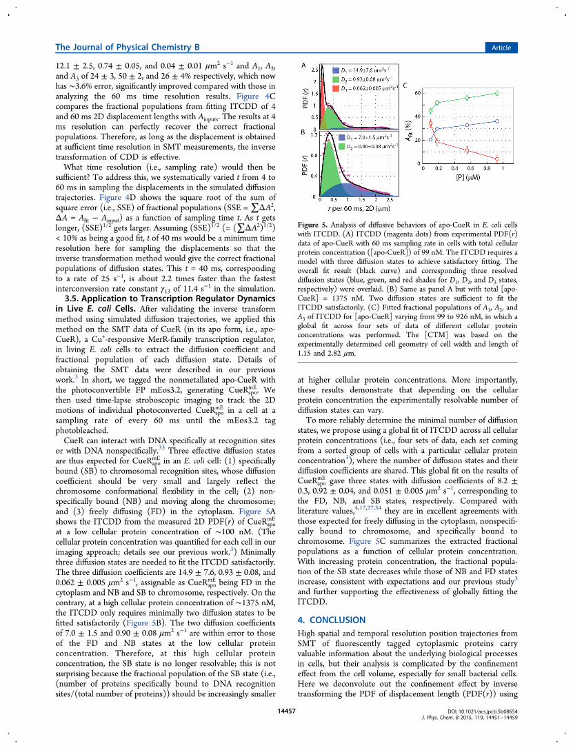
mE in an E. coli cell: (1) specificallybound (SB) to chromosomal recognition sites, whose diffusioncoefficient should be very small and largely reflect thechromosome conformational flexibility in the cell; (2) non-specifically bound (NB) and moving along the chromosome;and (3) freely diffusing (FD) in the cytoplasm. Figure 5Ashows the ITCDD from the measured 2D PDF(r) of CueRapo

mE

at a low cellular protein concentration of ∼100 nM. (Thecellular protein concentration was quantified for each cell in ourimaging approach; details see our previous work.3) Minimallythree diffusion states are needed to fit the ITCDD satisfactorily.The three diffusion coefficients are 14.9 ± 7.6, 0.93 ± 0.08, and0.062 ± 0.005 μm2 s−1, assignable as CueRapo

mE being FD in thecytoplasm and NB and SB to chromosome, respectively. On thecontrary, at a high cellular protein concentration of ∼1375 nM,the ITCDD only requires minimally two diffusion states to befitted satisfactorily (Figure 5B). The two diffusion coefficientsof 7.0 ± 1.5 and 0.90 ± 0.08 μm2 s−1 are within error to thoseof the FD and NB states at the low cellular proteinconcentration. Therefore, at this high cellular proteinconcentration, the SB state is no longer resolvable; this is notsurprising because the fractional population of the SB state (i.e.,(number of proteins specifically bound to DNA recognitionsites/(total number of proteins)) should be increasingly smaller

at higher cellular protein concentrations. More importantly,these results demonstrate that depending on the cellularprotein concentration the experimentally resolvable number ofdiffusion states can vary.To more reliably determine the minimal number of diffusion

states, we propose using a global fit of ITCDD across all cellularprotein concentrations (i.e., four sets of data, each set comingfrom a sorted group of cells with a particular cellular proteinconcentration3), where the number of diffusion states and theirdiffusion coefficients are shared. This global fit on the results ofCueRapo

mE gave three states with diffusion coefficients of 8.2 ±0.3, 0.92 ± 0.04, and 0.051 ± 0.005 μm2 s−1, corresponding tothe FD, NB, and SB states, respectively. Compared withliterature values,4,17,27,34 they are in excellent agreements withthose expected for freely diffusing in the cytoplasm, nonspecifi-cally bound to chromosome, and specifically bound tochromosome. Figure 5C summarizes the extracted fractionalpopulations as a function of cellular protein concentration.With increasing protein concentration, the fractional popula-tion of the SB state decreases while those of NB and FD statesincrease, consistent with expectations and our previous study3

and further supporting the effectiveness of globally fitting theITCDD.

4. CONCLUSIONHigh spatial and temporal resolution position trajectories fromSMT of fluorescently tagged cytoplasmic proteins carryvaluable information about the underlying biological processesin cells, but their analysis is complicated by the confinementeffect from the cell volume, especially for small bacterial cells.Here we deconvolute out the confinement effect by inversetransforming the PDF of displacement length (PDF(r)) using

Figure 5. Analysis of diffusive behaviors of apo-CueR in E. coli cellswith ITCDD. (A) ITCDD (magenta dots) from experimental PDF(r)data of apo-CueR with 60 ms sampling rate in cells with total cellularprotein concentration ([apo-CueR]) of 99 nM. The ITCDD requires amodel with three diffusion states to achieve satisfactory fitting. Theoverall fit result (black curve) and corresponding three resolveddiffusion states (blue, green, and red shades for D1, D2, and D3 states,respectively) were overlaid. (B) Same as panel A but with total [apo-CueR] = 1375 nM. Two diffusion states are sufficient to fit theITCDD satisfactorily. (C) Fitted fractional populations of A1, A2, andA3 of ITCDD for [apo-CueR] varying from 99 to 926 nM, in which aglobal fit across four sets of data of different cellular proteinconcentrations was performed. The [CTM] was based on theexperimentally determined cell geometry of cell width and length of1.15 and 2.82 μm.

The Journal of Physical Chemistry B Article

DOI: 10.1021/acs.jpcb.5b08654J. Phys. Chem. B 2015, 119, 14451−14459

14457

the confinement transformation matrix ([CTM]), building onthe previous work of Peterman30 on simulated single-statemembrane diffusions. Besides treating single-state cytoplasmicdiffusions, we further extended this method to analyzemultistate Brownian diffusions in the cytoplasm, includingboth noninterconverting and interconverting three-statediffusions. We demonstrated the effectiveness of this methodin determining the minimal number of diffusion states, theirdiffusion coefficients, and fractional populations as well as howto choose a sufficient time resolution in analyzing systemscontaining interconverting multistates. A successful applicationto experimental multistate SMT data of a transcription factor inlive E. coli cell is also demonstrated. Together with Peterman’searly work on membrane diffusion (whose extension tomultistate systems can readily follow our work on cytoplasmicdiffusion here), our method allows for direct connectionbetween SMT data with diffusion theory for analyzingmolecular diffusive behaviors in live bacteria.

■ ASSOCIATED CONTENT*S Supporting InformationThe Supporting Information is available free of charge on theACS Publications website at DOI: 10.1021/acs.jpcb.5b08654.

Validation of Brownian diffusion simulation and forwardtransformation of displacement length distribution in freespace with CTM. (PDF)

■ AUTHOR INFORMATIONCorresponding Author*E-mail: pc252@cornell.edu.Author Contributions†T.-Y.C. and W.J. contributed equally.NotesThe authors declare no competing financial interest.

■ ACKNOWLEDGMENTSWe acknowledge the National Institutes of Health (GM109993,AI117295, and GM106420) and Army Research Office(W911NF1510268) for funding and Erwin Peterman, ErnstL. M. Bank, and Felix Oswald for useful discussion on theconstruction of IPODD matrix.

■ REFERENCES(1) Leake, M. C.; Greene, N. P.; Godun, R. M.; Granjon, T.;Buchanan, G.; Chen, S.; Berry, R. M.; Palmer, T.; Berks, B. C. VariableStoichiometry of the Tata Component of the Twin-Arginine ProteinTransport System Observed by in Vivo Single-Molecule Imaging. Proc.Natl. Acad. Sci. U. S. A. 2008, 105 (40), 15376−15381.(2) Lillemeier, B. F.; Pfeiffer, J. R.; Surviladze, Z.; Wilson, B. S.;Davis, M. M. Plasma Membrane-Associated Proteins Are Clusteredinto Islands Attached to the Cytoskeleton. Proc. Natl. Acad. Sci. U. S. A.2006, 103 (50), 18992−18997.(3) Chen, T.-Y.; Santiago, A. G.; Jung, W.; Krzeminski, L.; Yang, F.;Martell, D. J.; Helmann, J. D.; Chen, P. Concentration- andChromosome-Organization-Dependent Regulator Unbinding fromDNA for Transcription Regulation in Living Cells. Nat. Commun.2015, 6, 7445.(4) Uphoff, S.; Reyes-Lamothe, R.; Garza de Leon, F.; Sherratt, D. J.;Kapanidis, A. N. Single-Molecule DNA Repair in Live Bacteria. Proc.Natl. Acad. Sci. U. S. A. 2013, 110 (20), 8063−8068.(5) Niu, L.; Yu, J. Investigating Intracellular Dynamics of FtszCytoskeleton with Photoactivation Single-Molecule Tracking. Biophys.J. 2008, 95 (4), 2009−2016.

(6) Javer, A.; Long, Z.; Nugent, E.; Grisi, M.; Siriwatwetchakul, K.;Dorfman, K. D.; Cicuta, P.; Cosentino Lagomarsino, M. Short-TimeMovement of E. Coli Chromosomal Loci Depends on Coordinate andSubcellular Localization. Nat. Commun. 2013, 4, 3003.(7) Axelrod, D.; Koppel, D. E.; Schlessinger, J.; Elson, E.; Webb, W.W. Mobility Measurement by Analysis of Fluorescence PhotobleachingRecovery Kinetics. Biophys. J. 1976, 16 (9), 1055−1069.(8) Hess, S. T.; Huang, S.; Heikal, A. A.; Webb, W. W. Biological andChemical Applications of Fluorescence Correlation Spectroscopy: AReview. Biochemistry 2002, 41 (3), 697−705.(9) Patterson, G.; Davidson, M.; Manley, S.; Lippincott-Schwartz, J.Superresolution Imaging Using Single-Molecule Localization. Annu.Rev. Phys. Chem. 2010, 61 (1), 345−367.(10) Mueller, F.; Stasevich, T. J.; Mazza, D.; McNally, J. G.Quantifying Transcription Factor Kinetics: At Work or at Play? Crit.Rev. Biochem. Mol. Biol. 2013, 48 (5), 492−514.(11) Solarczyk, K. J.; Zarębski, M.; Dobrucki, J. W. Inducing LocalDNA Damage by Visible Light to Study Chromatin Repair. DNARepair 2012, 11 (12), 996−1002.(12) Ries, J.; Schwille, P. Fluorescence Correlation Spectroscopy.BioEssays 2012, 34 (5), 361−368.(13) Small, A.; Stahlheber, S. Fluorophore Localization Algorithmsfor Super-Resolution Microscopy. Nat. Methods 2014, 11 (3), 267−279.(14) Hiramoto-Yamaki, N.; Tanaka, K. A. K.; Suzuki, K. G. N.;Hirosawa, K. M.; Miyahara, M. S. H.; Kalay, Z.; Tanaka, K.; Kasai, R.S.; Kusumi, A.; Fujiwara, T. K. Ultrafast Diffusion of a FluorescentCholesterol Analog in Compartmentalized Plasma Membranes. Traffic2014, 15 (6), 583−612.(15) Fernandez-Suarez, M.; Ting, A. Y. Fluorescent Probes for Super-Resolution Imaging in Living Cells. Nat. Rev. Mol. Cell Biol. 2008, 9(12), 929−943.(16) Yu, J.; Xiao, J.; Ren, X.; Lao, K.; Xie, X. S. Probing GeneExpression in Live Cells, One Protein Molecule at a Time. Science2006, 311, 1600−1603.(17) Elf, J.; Li, G.-W.; Xie, X. S. Probing Transcription FactorDynamics at the Single-Molecule Level in a Living Cell. Science 2007,316, 1191−1194.(18) Pinaud, F.; Clarke, S.; Sittner, A.; Dahan, M. Probing CellularEvents, One Quantum Dot at a Time. Nat. Methods 2010, 7 (4), 275−285.(19) Beausang, J. F.; Zurla, C.; Manzo, C.; Dunlap, D.; Finzi, L.;Nelson, P. C. DNA Looping Kinetics Analyzed Using DiffusiveHidden Markov Model. Biophys. J. 2007, 92 (8), L64−L66.(20) Chung, I.; Akita, R.; Vandlen, R.; Toomre, D.; Schlessinger, J.;Mellman, I. Spatial Control of Egf Receptor Activation by ReversibleDimerization on Living Cells. Nature 2010, 464 (7289), 783−787.(21) Das, R.; Cairo, C. W.; Coombs, D. A Hidden Markov Model forSingle Particle Tracks Quantifies Dynamic Interactions between Lfa-1and the Actin Cytoskeleton. PLoS Comput. Biol. 2009, 5 (11),e1000556.(22) Persson, F.; Linden, M.; Unoson, C.; Elf, J. ExtractingIntracellular Diffusive States and Transition Rates from Single-Molecule Tracking Data. Nat. Methods 2013, 10 (3), 265−269.(23) Michalet, X. Mean Square Displacement Analysis of Single-Particle Trajectories with Localization Error: Brownian Motion in anIsotropic Medium. Phys. Rev. E 2010, 82 (4), 041914.(24) Bosch, Peter J.; Kanger, Johannes S.; Subramaniam, V.Classification of Dynamical Diffusion States in Single MoleculeTracking Microscopy. Biophys. J. 2014, 107 (3), 588−598.(25) Robson, A.; Burrage, K.; Leake, M. C. Inferring Diffusion inSingle Live Cells at the Single-Molecule Level. Philos. Trans. R. Soc., B2013, 368 (1611), 20120029.(26) Blanco, M.; Johnson-Buck, A.; Walter, N. Hidden MarkovModeling in Single-Molecule Biophysics. In Encyclopedia of Biophysics;Roberts, G. K., Ed.; Springer: Berlin, 2013; pp 971−975.(27) Gebhardt, J. C. M.; Suter, D. M.; Roy, R.; Zhao, Z. W.;Chapman, A. R.; Basu, S.; Maniatis, T.; Xie, X. S. Single-Molecule

The Journal of Physical Chemistry B Article

DOI: 10.1021/acs.jpcb.5b08654J. Phys. Chem. B 2015, 119, 14451−14459

14458

Imaging of Transcription Factor Binding to DNA in Live MammalianCells. Nat. Methods 2013, 10 (5), 421−426.(28) Morisaki, T.; Muller, W. G.; Golob, N.; Mazza, D.; McNally, J.G. Single-Molecule Analysis of Transcription Factor Binding atTranscription Sites in Live Cells. Nat. Commun. 2014, 5, 4456.(29) Bakshi, S.; Choi, H.; Mondal, J.; Weisshaar, J. C. Time-Dependent Effects of Transcription- and Translation-Halting Drugs onthe Spatial Distributions of the Escherichia Coli Chromosome andRibosomes. Mol. Microbiol. 2014, 94 (4), 871−887.(30) Oswald, F.; L. M. Bank, E.; Bollen, Y. J. M.; Peterman, E. J. G.Imaging and Quantification of Trans-Membrane Protein Diffusion inLiving Bacteria. Phys. Chem. Chem. Phys. 2014, 16 (25), 12625−12634.(31) Elowitz, M. B.; Surette, M. G.; Wolf, P.-E.; Stock, J. B.; Leibler,S. Protein Mobility in the Cytoplasm Ofescherichia Coli. J. Bacteriol.1999, 181 (1), 197−203.(32) Zhang, M.; Chang, H.; Zhang, Y.; Yu, J.; Wu, L.; Ji, W.; Chen, J.;Liu, B.; Lu, J.; Liu, Y.; et al. Rational Design of True Monomeric andBright Photoactivatable Fluorescent Proteins. Nat. Methods 2012, 9(7), 727−729.(33) Joshi, C. P.; Panda, D.; Martell, D. J.; Andoy, N. M.; Chen, T.-Y.; Gaballa, A.; Helmann, J. D.; Chen, P. Direct Substitution andAssisted Dissociation Pathways for Turning Off Transcription by aMerr-Family Metalloregulator. Proc. Natl. Acad. Sci. U. S. A. 2012, 109,15121−15126.(34) Mehta, P.; Jovanovic, G.; Lenn, T.; Bruckbauer, A.; Engl, C.;Ying, L.; Buck, M. Dynamics and Stoichiometry of a RegulatedEnhancer-Binding Protein in Live Escherichia Coli Cells. Nat.Commun. 2013, 4, 1997.

The Journal of Physical Chemistry B Article

DOI: 10.1021/acs.jpcb.5b08654J. Phys. Chem. B 2015, 119, 14451−14459

14459