quantifying sources & sinks of atmospheric co...

Uptake and Storage of Anthropogenic Carbon

by

Christopher L. Sabine ; NOAA/PMEL, Seattle, WA USA

Acknowledgements: Richard A. Feely (PMEL), Frank Millero (RSMAS), Andrew Dickson (SIO), Rik Wanninkhof (RSMAS), Toste Tanhua (IFM-geomar), Taro Takahashi (LDEO) , Niki Gruber (ETH Zürich)

Quantifying Sources & Sinks of Atmospheric CO2

OUTLINE

1. Briefly review how observations contribute to Carbon uptake estimates

2. Describe how we determine ocean carbon inventories

3. Consider issues for understanding future ocean carbon uptake and storage

4.Suggest an approach for where we go from here

Carbon Inventories of Reservoirs that Naturally Exchange Carbon on Time Scales of Decades to Centuries

Ocean38,136 PgC

Soil=2300 PgC

Plants=650 PgCAtm.=775 PgC

Preind.Atm. C=76%

Ocean Anth. C=0.35%

Oceans contain ~90% of carbon in this 4 component system

anthropogenic component is difficult to detect

Anth. C=24%

adapted from Sabine et al., 2004

Global Carbon Budget for 2000-2005

Air-sea Flux

Based on ~3 million measurements since 1970 and NCEP/DOE/AMIP II reanalysis.Global flux is 1.4 ±0.7 Pg C/yr

Takahashi et al., Deep Sea Res. II, 2009

Takahashi climatological annual mean air-sea CO2 flux for reference year 2000

Surface CO2 observation network

Global Surface CO2 observations by year

Based on SOCAT version 1 Jan. 2010

The number of annual measurements has been increasing exponentially since for the last 50 years

A focus on studying ocean carbon in the 1990s led to the instrumenting of many more research ships

The dramatic increases in the 2000s can be attributed to the instrumenting of commercial shipsFrom Sabine et al., 2010

New Technologies can Help Expand the Surface CO2 Observation Network

One Example: Integrated MapCO2/Wave Glider system under development

Producing Seasonal CO2 Flux Maps

In situ samplingpCO2, SST, SSS

Remote sensing SST, color & windSoon SSS

Algorithm developmentpCO2= f(SST, color)

Co-located satellite data

Regional satellite SST & color data

Apply algorithm toregional SST& color fields to obtain seasonal pCO2maps

Algorithm development Gas transfer, k =f (U10,SST)

Wind data

pCO2 maps

Flux maps

Flux = k s ∆pCO2

Global Flux Map suggests an interannual variability of 0.23 Pg C

Surface observations have large variability over a wide range of time and space scales making it very difficult to properly isolate the anthropogenic increases. Uptake of 2 Pg C yr-1 only requires a ∆pCO2 of 8ppm.

Several Independent Approaches are Converging on an Estimate of the Anthropogenic CO2 Uptake

Table 1. Summary of Recent Estimates of the Oceanic Uptake Rate of Anthropogenic CO 2for the Period of the 1990s and Early 2000saCgP(etamitsEdohteM 1 srohtuAdoirePemiT)

Estimates Based on Oceanic ObservationsOcean Inversion (10 models) 2.2 ± 0.3 Nominal 1995 this study and Mikaloff - Fletcher et al. [2006]Ocean Inversion (3 models) 1.8 ± 0.4 Nominal 1990 Gloor et al. [2003]Air-sea pCO2difference (adjusted)a 1.9 ± 0.7 Nominal 2000b Takahashi et al. [2008]Air-sea pCO2difference (adjusted)a,c 2.0 ± 60% Nominal 1995 Takahashi et al. [2002]

Estimates Based on Atmospheric ObservationsAtmospheric O2/N2 ratio 1.9 ± 0.6 1990–1999 Manning and Keeling [2006]Atmospheric O2/N2 ratio 2.2 ± 0.6 1993–2003 Manning and Keeling [2006]Atmospheric O2/N2 ratio 1.7 ± 0.5 1993–2002 Bender et al. [2005]Atmospheric CO2inversions (adjusted) a 1.8 ± 1.0 1992–1996 Gurney et al. [2004]

Estimates Based on Oceanic and Atmospheric ObservationsAir-sea13C disequilibrium 1.5 ± 0.9 1985–1995 Gruber and Keeling [2001]Deconvolution of atm. δ13C and CO2 2.0 ± 0.8 1985–1995 Joos et al. [1999a]Joint atmosphere-ocean inversion 2.1 ± 0.2 1992–1996 Jacobson et al. [2007b]

Estimates Based on Ocean Biogeochemistry ModelsOCMIP-2 (13 models) 2.4 ± 0.5 1990–1999 Watson and Orr [2003]OCMIP-2 (4 ‘‘best’’ models)d 2.2 ± 0.2 1990–1999 Matsumoto et al. [2004]a Adjusted by 0.45 Pg C a 1 to account for the outgassing of natural CO2that is driven by the carbon input by rivers.b The estimate for a nominal year of 1995 would be less than 0.1 Pg C a 1smaller.c Corrected for wrong windspeeds used in published version; see http://www.ldeo.columbia.edu/res/pi/CO2/carbondioxide/pages/air_sea_flux_r ev1.html.d These models were selected on the basis of their ability to simulate correctly, within the uncertainty of the data, the observed oceanic inventories and

regional distributions of chlorofluorocarbon and bomb radiocarbon.

From Gruber et al., Glob. Biogeochem. Cy., V 23, doi:10.1029/2008GB003349, 2009

Inventorychanges



Tropical Pacific shows up as a significant sink for CO2 despite the fact that net fluxes are out of the ocean and inventory estimates show a minimum near the equator

An example of the differences between uptake and storage can be found in the Tropical Pacific

Gruber et al. 2009

Column inventory of anthropogenic CO2 that has accumulated in the ocean between 1800 and 1994 (mol m-2) based on ∆C* approach

Mapped Inventory =106±17 Pg C; Global Inventory =118±19 Pg C

22 Pg C 40 Pg C44 Pg C

Shipboard Sampling for Ocean Carbon

GEOSECS Station Locations

6,037 carbon samples with a DIC uncertainty ~ 20 µmol kg-1

Much of our understanding of the modern ocean carbon cycle was based on the GEOSECS program of the 1970s.

85

127

170

212

106

148

191

Ant

hrop

ogen

ic C

O2

Inve

ntor

y (P

g C

)

Atmospheric data from SIO and ESRL courtesy of P. Tans

Brewer1978

Chen &Millero1979

GEOSECS: the first global, documented, high precision ocean carbon measurements

"...unless [inorganic carbon] measurements that are more accurate by an order of magnitude can be made, at least a decade will pass before direct confirmation of the model-based [fossil fuel CO2 uptake] estimates will be obtained."

Broecker et al., Science, 206, p. 409, 1979GEOSECS

1972-1978

In the early 1990s the World Ocean Circulation Experiment (WOCE), the Joint Global Ocean Flux Study (JGOFS), and the NOAA/OACES program

joined forces to conduct a global survey of CO2 in the oceans.

>70,000 sample locations; DIC ± 2 µmol kg-1; TA ± 4 µmol kg-1

http://cdiac.esd.ornl.gov/oceans/glodap/Glodap_home.htm

Improved accuracy attributed to:1. Refinement of coulometric DIC and SOMMA

by K. Johnson2. Development of CRMs by A. Dickson

85

127

170

212

106

148

191

Ant

hrop

ogen

ic C

O2

Inve

ntor

y (P

g C

)

90+/- ~40 Pg C(Chen, 1993)

118+/- 19 Pg C(Sabine et al, 2004)


Brewer1978

Chen &Millero1979

Gruberet al.1996

It was almost 20 years later before an improved anthropogenic CO2 technique developed

WOCEJGOFS

1989-1998GEOSECS1972-1978

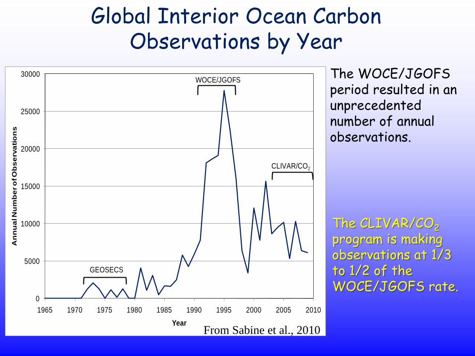
Global Interior Ocean Carbon Observations by Year

0

5000

10000

15000

20000

25000

30000

1965 1970 1975 1980 1985 1990 1995 2000 2005 2010

An

nu

al N

um

ber

of O

bse

rvat

ion

s

Year

GEOSECS

WOCE/JGOFS

CLIVAR/CO2

The WOCE/JGOFS period resulted in an unprecedented number of annual observations.

The CLIVAR/CO2program is making observations at 1/3 to 1/2 of the WOCE/JGOFS rate.

From Sabine et al., 2010

85

127

170

212

106

148

191

Ant

hrop

ogen

ic C

O2

Inve

ntor

y (P

g C

)

90+/- ~40 Pg C(Chen, 1993)

GEOSECS1972-1978

WOCEJGOFS

1989-1998

118+/- 19 Pg C(Sabine et al, 2004)

?

Moving beyond total carbon inventories…

CLIVAR2003-2012


Comparison of the Change in Anthropogenic C Inventory over two decadal periods

The GEOSECS-WOCE changes were re-evaluated using the exact same techniques used for the WOCE-CLIVAR changes for these calculations.

Anthropogenic carbon inventory increases were higher at all latitudes over the last decade than the average increases between GEOSECS and WOCE

# Data from: Time period Method

a (Peng et al 1998) 1978-1995 Isopycnal, O2 adjusted

b (Tsunogai et al 1993) 1974-1991 Column integrated change in

preformed carbonte

c (Peng et al 2003) 1973-1991 MLR

d (Sabine et al 2008) 1991/2 – 2005/6

1994 - 2004

eMLR

e (Murata et al 2009) 1993-2005 Isopycnal, O2 adjusted

f (Matear & McNeil 2003) 1968-1991/1996 MLR

g (Murata et al 2007) 1992-2003 Isopycnal, O2 adjusted

h (Friis et al 2005) 1981-1997/99 eMLR

i (Olsen et al 2006) 1981-2002/03 eMLR

j (Tanhua et al 2007) 1981-2004 eMLR

k (Murata et al 2008) 1992/93-2003 Isopycnal, O2 adjusted

Individual assessments of decadal carbon changes all show increasesthe patterns of change are complicated

Sabine and Tanhua 2009

Interim Results Have Shown:1. On decadal scales, changes in ocean circulation can

have a significant and sometimes dominant impact on carbon inventory changes.

2. The decadal patterns of anthropogenic carbon storage do not necessarily follow the long term storage pattern.

illusion chaos relieftime

truth(what is the vulnerability

of the marine

biological pump?)

I believe we are in a situation similar to the model evolution proposed by Corinne LeQuere a few years back

Adapted from C. LeQuere

Long-term storage Individual

assessmentsCoordinated

global assessment

Annual Change in Ocean C Storage

I believe we are in a situation similar to the model evolution proposed by Corinne LeQuere a few years back

3 400Anthropogenic CO2 uptake

Anthrop

ogen

icCO

2up

take

rate

(PgCyr

–1)

Atm

osph

ericCO

2(p.p.m

.)

Atmospheric CO2

IPCC consensus estimates380

360

340

320

300

280

2.75

2.5

2.25

2

1.75

1.5

1.25

1

0.75

0.5

0.25

01775 1800 1825 1850 1875

Time (yr AD)1900 1925 1950 1975 2000

Figure 2 Anthropogenic carbon uptake rate from 1765 to 2008 (blacksolid line). The shaded area represents the error envelope (see Fig. 1 legend).Also shown are the decadal average uptake rates adopted by the IPCC fourth-assessment report (AR4)4 (blue circles; vertical error bars are6 1 s.d. andhorizontal error bars span the averaging period of years) and theatmospheric CO2 mixing ratio29 used for the inversion (red dashed line).

Katiwala et al., Nature, Nov. 2009

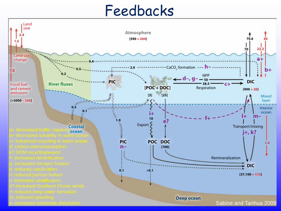
Feedbacks

Coastalocean

Mixedlayer

Interiorocean

Deep ocean

Fossil fueland cementemissions

[>5000 – 330]

Landsink

Land-usechange

[900 + 20]

[3]

[37,100 + 115]

Atmosphere[590 + 204]

River fluxes

NPP

Respiration[POC + DOC][25]

PIC

DOC[700]

POCPIC

DIC

DIC

0.50.5

1.41.4

10

22

2.0 CaCO3 formation

Remineralization

Export Transport/mixing

g–h–

n–

j+, k?

l+ m–f+

j+, k?

(h)+i+

0.40.4

0.20.2

2.4

1.5

2.4

0.3

1.9

0.1

1.5

7.27.2

0.3

1.9

0.1

0.1 <0.10.1 <0.1

70.6

70

20

22.2

70.6

70

20

22.2

a)+

(b)+

a+

b+

l+ m–

38.55038.550

(c)d–, g–d–, g–

c+

f+e?e?10

a+ decreased buffer capacityb+ decreased solubility in warm oceanc+ enhanced recycling in warm oceand- carbon overconsumptione? DOM recycling/exportf+ increased denitrificationg- increased nitrogen fixationh- reduced calcificationi+ reduced particle ballastj+ increased stratificationk? increased Southern Ocean windsl+ reduced deep water formationm- reduced upwellingn- increased carbonate dissolution Sabine and Tanhua 2009

Pre

indu

stria

l

All Buffer Factors show a minimum where DIC=Alk

As CO2 increases, North Pacific subtropical gyre waters are approaching

the buffer minimum

Mod

ern

2x C

O2

3x C

O2

Egleston et al. (GBC, 2010)

2HCO3–CO3

2–CO2(aq) + H2O +

+ H+CO2(aq) + H2O HCO3–

Higher buffer factor means larger DIC increase for the same amount of CO2 rise

Preindustrial

PreindustrialModern

25% drop in uptake


PreindustrialModern

2X CO2

60% drop in uptake


PreindustrialModern

2X CO23X CO2

75% dropin uptake


coastalexchanges



Summary and Challenges-Surface ocean observations and modeling are increasing and improving

our ability to constrain the air-sea fluxes (uptake)

*This is still being done in an ad hoc manner and we will not be able to reach needed accuracy without better coordination and embracing new technologies

- Ocean interior measurements and modeling (inventories) compliment the uptake estimates and provide information on feedbacks

* These observations are personnel and infrastructure intensive thus they are not well supported with their current funding through research

- Coastal exchanges are not well understood

* Currently there is no coordinated effort to improve our understanding

- The above observing systems may also be able to address verification of ocean carbon capture and storage approaches

* However, the current programs are not optimized for this.

quantifying sources & sinks of atmospheric co...

Documents