quantifying the biotic enhancement of mineral weathering
TRANSCRIPT

1
Quantifying the Biotic Enhancement of Mineral Weathering by Moss
Michael John Collingwood Crouch
Thesis presented in part-fulfilment of the degree of Master of Science by Research in accordance with the regulations of
The University of East Anglia
School of Environmental Sciences University of East Anglia University Plain Norwich NR4 7TJ UK March 2010
© 2010 Michael John Collingwood Crouch
This copy of the thesis has been supplied on the condition that anyone who consults it is understood to recognise that its copyright rests with the author and that no quotation from the thesis, nor any information derived therefrom, may be published without the author’s prior written consent.
2
“Life improves the capacity of the environment to sustain life… Life makes
needed nutrients more readily available…through the tremendous chemical
interplay from organism to organism.”
Extract from Frank Herbert‟s „Dune‟, 1965.
3
Abstract
Addressing the paucity of reliable, robust studies into the weathering effect exerted by biota
onto rocks and minerals: mineral weathering by the moss Physcomitrella patens was measured
in a novel in vitro microcosm study.
A sterile technique was maintained in order to ensure that P. patens was the only organism
exerting weathering affects within the microcosms, control microcosms were devoid of biota
entirely. After the weathering period ( x = 112 days) the moss and aqueous solutions resulting
from microcosms were analysed for Al, Ca, Fe, K, Mg, Na and Si using Inductively Coupled
Plasma - Atomic Emission Spectroscopy (ICP-AES) and for PO43-
and SiO44-
using a Nutrient
Auto-Analyser.
Results show strong biotic enhancements for all ICP analytes and PO43-
(except Na). Biotic
enhancements were strongest for Fe on most substrates, reaching levels of <625x abiotic
weathering in andesite microcosms ( = 330.7x) and <493.6x on granite (all significant at
P<0.01). Aqueous phase biotic enhancements for PO43-
were 5.3x on vermiculite and 4.2x on
granite.
Experimental substrates were analysed using X-Ray Fluorescence Spectroscopy (XRF) in
order to ascertain their petrologies and to enable comparison with weathering results to
determine whether ions were being preferentially weathered over their baseline levels.
Weathering of plant macronutrients is enhanced over the baseline stoichiometries, but biotic
influence on this effect appears negligible.
This study has a bearing upon hypotheses linking the effects of increased land-surface
weathering to the Ordovician glaciation due to the proliferation of bryophyte organisms across
the land surface. Furthermore this study finds that P. patens is an excellent model bryophyte
for studies of weathering as well as its more common use as the model bryophyte in genetic
studies.
Keywords: Biogeochemistry, Enhancement, Microcosm, Mineral, Moss, Weathering.

4
Table of Contents
Section Start Page
I: Figures, Tables and Equations 5
II: Acknowledgements 11
1: Introduction 13
2: Experimental Methods 35
3: Analytical Methods 53
4: Results and Discussion 76
5: Conclusions 132
6: List of References 142
Index to Appendices 147

5
I: Figures, Tables and Equations
Figures
Figure
Description Page
1.1 Earth‟s continents during the Upper Ordovician 15
1.2 The Long-Term Carbon Cycle 17
1.3 δ13
C excursions and stratigraphy in the Ordovician 21
1.4 Moss life cycle 23
1.5 Sheet and framework silicates 29
1.6 Side and plan views of a basalt microcosm 32
2.1 Flow chart – key stages in the experimental procedure 36
2.2 Flow chart – substrate and microcosm preparation 38
2.3 Flow chart – sample preparation and sample analysis 42
2.4 Photomicrographs of moss and on vermiculite clasts 43
2.5 Flow chart – the Biomass Oxidation Method 45
2.6 Flow chart – moss tissue culturing procedure 50
2.7 Flow chart – moss inoculum and filtrate preparation 51
3.1 Calibration plot for Al in ICP Round 10 57
3.2 Graph – Log plot of mean ICP analytical precision 58
3.3 Flow chart – microcosmal data work up 60
3.4 Frequency distribution – log normal 63
3.5 Frequency distribution – Gaussian (+ve skew) 64
3.6 Frequency distribution – Gaussian 64
3.7 NAA silicate calibration 28/4/09 66
3.8 NAA phosphate calibration 31/3/09 67
3.9 NAA chart recorder paper, mal-formed peaks 68

6
Figures (Continued)
Figure
Description Page
3.10 Colour changes – silicate/phosphate reagents + H2O2 69
3.11 Absorbencies across visual spectrum – hydrogen peroxide 70
3.12 Absorbencies across visual spectrum – nitric acid 71
3.13 Flow chart – NAA data work-up 72
3.14 Flow chart – fusion bead preparation 73
3.15 Flow chart – XRF data work up 75
4.1 Side and plan views of a control granite microcosm 79
4.2 Plan and side views of mossed granite microcosms 80
4.3 Graph – Granite aggregated amounts weathered (μmol) 81
4.4 Graph – Granite aggregated normalised weathering 83
4.5 Preferential uptake and purging of analytes by moss 84
4.6 Graph – Granite aggregated PO4 and SiO4 weathering 85
4.7 Graph – 24/6/08 Granite, normalised weathering 87
4.8 Graph – 12/1/09 Granite, normalised weathering 88
4.9 Side and plan views of a control andesite microcosm 90
4.10 Plan and side views of a mossed granite microcosms 91
4.11 Graph – Andesite aggregated amounts weathered (μmol) 92
4.12 Graph – Andesite aggregated normalised weathering 93
4.13 Graph – 2/12/08 Andesite, normalised weathering 95
4.14 Graph – 25/1/09 Andesite, normalised weathering 96
4.15 Graph – Vermiculite aggregated amounts weathered (μmol) 99
4.16 Graph – Vermiculite aggregated normalised weathering 100
4.17 Graph – Vermiculite PO4 and SiO4 weathering 102
4.18 Graph – 24/6/08 Chlorite amounts weathered (μmol) 104
4.19 Graph – 24/6/08 Chlorite, normalised weathering 105

7
Figures (Continued)
Figure
Description Page
4.20 Graph - 30/7/09 Inoculum Only vs. Granite 108
4.21 Graph - 30/7/09 Inoculum Only vs. Granite (normalised) 109
4.22 Graph - Amounts of Fe in Wmoss (μmol) against mass of moss (mg) 115
4.23 Graph - Amounts of Si in Wb (μmol) against mass of moss (mg) 115
4.24 Graph - Amounts of Fe in Wmoss (μmol s-1
mg-1
) against mass of
moss (mg)
116
4.25 Graph - Amounts of Fe in Wb (μmol s-1
mg-1
) against mass of moss
(mg)
116
4.26 Substrate petrology and stoichiometries of the microcosmal
fractions
123
5.1 Biotic weathering series 133
Tables
Table Description Page
1.1 Geologic time in the Ordovician 15
1.2 Eight nutrient elements essential for moss growth 26
1.3 The mineral nutrients arranged highest/lowest by cocn. 27
1.4 The experimental substrates and their petrologies 30
2.1 The experimental substrates 37
2.2 The microcosm experiments 41
2.3 The microcosm water sampling methods 46

8
Tables (Continued)
Table Description Page
3.1 ICP-AES analytes and emission wavelengths 55
3.2 ICP-AES standards 56
3.3 Standard concentrations 56
3.4 ICP analytical precision 58
3.5 Interference determination experiment – sample labelling 70
3.6 XRF analytes 74
4.1 P values – Wtot vs. Wa, granite aggregated dataset 84
4.2 P values – Wb vs. Wa, granite aggregated dataset 86
4.3 P values – Wtot vs. Wa, andesite aggregated dataset 94
4.4 P values – Wtot vs. Wa, vermiculite aggregated dataset 101
4.5 P values – Wb vs. Wa, vermiculite aggregated dataset 102
4.6 P values – Wtot vs. Wa, 24/6/08 chlorite experiment 106
4.7 P values – Wtot granite vs. Wtot bare 110
4.8 Mean amounts of moss recovered from mossed „cosms 111
4.9 Wmoss per mg of moss biomass – granite aggregated 112
4.10 Wmoss per mg of moss biomass – andesite aggregated 113
4.11 Wmoss per mg of moss biomass – vermiculite aggregated 113
4.12 Wmoss per mg of moss biomass – 24/6/08 chlorite 114
4.13 Mean mass of moss obtained from jiffys (optimum conditions) 114
4.14 Amount of analytes in 3 substrates with ref. values (XRF) 118
4.15 Mean amounts of majors within substrates (XRF, μmol g-1
) 119
4.16 Mean amounts of majors normalised to Fe 119
4.17 Stoichiometry of granite substrate and microcosmal components
(relative to Fe)
124
4.18 Stoichiometry of andesite substrate and microcosmal components
(relative to Fe)
125

9
Tables (Continued)
Table Description Page
4.19 Minimum ionic radii for the experimental analytes 127
4.20 Comparison between error bars and U test P values 130
5.1 Biotic enhancement of weathering (Ψ) values of all analytes on all
substrates (with P values)
132
5.2 Bryophyte colonisation scenarios 134
5.3 Fluxes of analytes from moss-colonised granite (mol/m2) 135
5.4 Fluxes of analytes from moss-colonised granite (mol/m2/s) 135
5.5 Fluxes of analytes from Ordovician land surface under different
colonisation scenarios
135
Equations
Equation
Description Page
1.1 The Urey reactions 16
1.2 An example of the Urey reactions 17
1.3 Mass balance of δ13
C 19
1.4 Isotopic fractionation formula 19
1.5 Total weathering 33
1.6 Actual equation for total weathering (Wtot) 33
1.7 Calculation for net biotic weathering (Wnetbio) 34
1.8 Biotic Enhancement of Weathering (Ψ) calculation 34

10
Equations (Continued)
Equation
Description Page
4.1 Standard Error calculation 76
4.2 Equation for calculating 95% confidence interval 77
4.3 Stoichiometric formulae of four substrates 120
4.4 Stoichiometric formula of typical dry plant tissue 121
4.5 Stoichiometric formulae of moss inoculums at initial conditions 121
4.6 Stoichiometric formula of filtrate at initial conditions 122
5.1 Formula for calculating flux of analyte (mol/m2) per unit Earth
surface
136

11
II: Acknowledgements
First and foremost: I sincerely thank Martin Johnson for his coaching and mentoring (and for
the large amount of time that he spent on these two tasks). It is no under-statement to say that
the rigour of a number of the methodologies used in this study (particularly the blank taking
procedure) and the quality of this thesis would be much the poorer were it not for Martin‟s
helpful input. Similarly: I also sincerely thank Nuno Pires: Nuno conducted a lot of the early
pilot work into the moss/mineral microcosms and trained me in a number of the requisite lab
skills (sterile technique, tissue culturing etc.) I kindly thank Liam Dolan and Tim Lenton for
their supervision, for having confidence in my abilities and for persuading me (at times) to get
on with the things that mattered! I also thank Liam for sacrificing two of his holiday souvenirs
for use as experimental substrates. Furthermore I thank my examiners: Alayne Street-Perrott
and Brian Reid for their comments that helped to improve the final draft of this thesis.
For their warm welcome to The John Innes Centre (JIC), for showing me the ropes and
generally creating a good atmosphere I thank the „Rooties‟. I also thank Tom Moore, Emma
Greer and Heather Kingdom: Tom got me on the bar rota and Heather created the monster that
is „DJ Crouchie McGroovin‟! Great times.
Brian Reid was particularly helpful in recommending a safe method for oxidising plant tissue
which set me off of the right track with the moss biomass oxidation method development.
Julian Andrews provided some very useful advice on petrology and appropriate methods of
analysis as did Tom Bell on how to treat non-detects in a dataset. I thank Colin Goldblatt for
bringing me some rocks back from the Lake District and Paul Disdle for showing me how to
cut them up. I also thank Rich Boyle for many stimulating discussions on weathering!
For their expertise on matters analytical I thank Graham Chilvers (ICP Spectroscopy
Technician), Keith Weston, Kim Wright and Jim Hunter (Nutrient Auto-Analyser). I also
thank Bertrand Lézé (Technician i/c XRF). People at JIC who deserve special thanks include
Roy Dunford for general advice and helping me find things and Andrew Davis who took
superb photos of the microcosms. I also thank Mary-Anne Sangarde and her team in media
preparation and Gary Creissen who conducted the light measurements. I kindly thank ELSA
(Earth & Life System Alliance) for funding bench fees, instrumental and some consumable

12
costs and for allowing me to be a part of such an exciting collaboration. I am sure that the
future of the Alliance will be an extremely bright one indeed.
At a personal level I thank my friends for their support: particularly Matt Tucker, Alys Earl,
Beth Bradshaw, Sophie Fleming, Antoine Peraldi, Matt Watkins, Karina Hudek, The Paxtons
and anybody else who supported and encouraged me. I also thank my brother for his periodic,
stupid text messages (and for answering mine) and Nan and Malc for their support. Finally; I
thank my Mum and Dad for funding and for putting up with all my seemingly recondite
enthusiasms over the years!

13
1: Introduction
1.1 Motivation and Impetus for this Study
The motivation for this study was a need to determine whether or not moss weathers (breaks
down as a result of its growth) various rocks and minerals and, if the moss does weather the
rock, to determine the factor of increase of this weathering. This factor of increase is known as
the „Biotic Enhancement of Weathering‟ (e.g. Aghamiri & Schwartzman (2002) and Lenton &
Watson (2004)).
The impetus for conducting this study was the need to test a novel hypothesis of Prof. Tim
Lenton1 and Prof. Liam Dolan
2 that a glaciation in the late Ordovician period of Earth‟s
history was caused by the effects of increased land-surface weathering by bryophyte-like
organisms (bryophytes are a division of the kingdom Plantae which includes mosses). A
number of pre-existing hypotheses link the late Ordovician with increased weathering but
these hypotheses vary in nature (see Section 1.4, hereafter the „§‟ symbol is used to denote a
section).
There is a paucity of studies into the effects of biota upon mineral weathering (as noted by
Schwartzman (2000) and Berner (2004)). From the formation of Geology as a discipline in its
own right (circa the mid-18th
Century) up until as recently as the late 1960s; the potential of
biota as an important force for denuding and altering minerals and providing useful chemicals
for other, evolving biota was largely unrecognised (Street-Perrott & Barker (2008); Hazen
(2009)). Credit must be given to Vladimir Vernadsky, G. Evelyn Hutchison, Thomas Lovering
and James Lovelock for trying to initiate a less reductionist approach to geology over this
period. This dogma occurred largely as a product of a prevailing reductionist method that
caused geologists to centre on more physical processes (such as vulcanism) to the detriment of
studies into biota. Such a situation need not have occurred had geologists heeded more closely
the words of a man often described as „The Father of Geology‟, James Hutton. Hutton once
wrote that he considered “the Earth to be a super-organism and that its proper study should be
by physiology” (cit. in Lovelock (1979); UNU (1992)). In other words Hutton advised that a
1 School of Environmental Sciences, University of East Anglia, NR4 7TJ, UK.
2 Now at: Department of Plant Sciences, University of Oxford, OX1 3RB, UK.

14
non-reductionist, systems-based approach should be adopted when studying the Earth. This
study will attempt to emulate such an approach.
1.2 The Ordovician
1.2.1 Introduction
The Ordovician is a system period in geological time that lasted between 488.3Ma (±1.7)
(Million years ago) and 443.7Ma (±1.5) (NB all ages used in this thesis shall be those of
Gradstein et al. (2004), as approved by the International Commission on Stratigraphy (ICS)).
During the Upper Ordovician (460.9Ma ±1.6 to 443.7Ma ±1.5) the southern continents
collected into a single supercontinent known as Gondwana (Crowley & Baum, 1991) (See
Figure 1.1).
1.2.2 Glaciation
The precise onset of the Ordovician glaciation, the causes and the length of its duration are
subject to debate (e.g. Brenchley et al. (1994); Pope & Steffen (2003), arguing for a short and
long glaciation respectively). One point of consensus is that the Ordovician glaciation is
unique in Earth‟s history in that its onset occurred during a period when the partial pressure of
atmospheric carbon dioxide (pCO2) was high (Pope & Steffen, 2003). Estimates vary, but
pCO2 in the Ordovician is estimated at 10-18 times greater than the Present Atmospheric Level
(PAL) (Op. cit., Yapp & Poths (1992)).

15
System Period
Series Epoch
Stage Age at start (Ma)
Error (±Ma)
Silurian
Ordovician
Upper Hirnantian 445.6 1.5
Katian 455.8 1.6
Sandbian 460.9 1.6
Middle Darriwilian 468.1 1.6
Dapingian 471.8 1.6
Lower Floian 478.6 1.7
Tremadocian 488.3 1.7
Cambrian
Table 1.1 – Geologic Time in the Ordovician (After Gradstein et al. (2004)).
It was previously thought that the Ordovician glaciation was a short-lived (<1Ma) event in the
Hirnantian (see Table 1.1) (e.g. Brenchley et al. (1994)), there is however an increasing body
of evidence that the glaciation began in the Middle Ordovician and ended in the late
Hirnantian (e.g. Pope & Steffen (2003); Saltzman & Young (2005)). Such hypotheses are
based on isotopic ratios contained within sediments formed in the Ordovician through a
science known as Chemostratigraphy (see §1.4). Figure 1.1 (below) shows the position of
Earth‟s continents in the late Ordovician
Figure 1.1 – Earth’s continents during the Upper (late) Ordovician (≈450 million years ago) represented as a Mercator’s projection. During the Upper Ordovician the southern
continents gathered to form a single supercontinent: Gondwana. Graphic reproduced from Blakey (2009).3
3 Reproduced under a Creative Commons Attribution ShareAlike 3.0 license.

16
1.3 The Geochemistry of Weathering and the Long-Term Carbon Cycle
As a plant grows its rootlets secrete organic acids and chelates which break down nutrient
cations (Moulton & Berner, 1998). Upon the death of the plant (or parts of it) the decay of
organic matter produces further organic acids and carbonic acid (H2CO3) (Op. cit.) These
effects can be termed „Biotic Weathering‟. Weathering can also occur due to abiotic effects,
for example: atmospheric carbon dioxide dissolving in water also forms carbonic acid (the
affect of this reaction is likely to have been more important in the Ordovician period when the
pCO2 was higher than PAL).
Biotic weathering occurs as a result of physical and chemical effects; physical effects include
the hydraulic pressure of plant roots breaking a substrate apart whereas chemical weathering
refers to the hydrolysis of minerals by acids (Graham et al., 2010). The focus of this thesis will
be upon chemical weathering (the hydrolysis of minerals by acids, in this case resulting from
mosses) though it is important to note that the two processes do not operate independently of
each other.
Mineral weathering of calcium and magnesium-silicate compounds leads to the liberation of
calcium and magnesium cations (Ca2+
and Mg
2+) which in a three-stage reaction with
atmospheric CO2 forms two bicarbonate ions (2HCO3-). These reactions are known as the
Urey reactions (after Harold Urey 1893-1981). If CO2 (g) is taken to react with a generalised
Calcium-Silicate mineral (CaSiO3), the reactions that take place can be represented as shown
in Equation 1.1 (below).
1: 2CO2 + 3H
2O + CaSiO
3 → Ca
2+
+ 2HCO3
-
+ H4SiO
4
2: Ca
2+
+ 2HCO3
-
→ CaCO3 + CO
2 + H
2O
3: H4SiO
4 → SiO
2 + 2H
2O
CO2
+ CaSiO3
→ CaCO3
+ SiO2
Equations 1.1 – The Urey reactions (Berner, 2004), the sum of all three reactions given in bold. Note that for every two moles of CO2 (g) only one mole is sequestered in these reactions.

17
If this reaction is applied to a calcium bearing plagioclase the following reaction occurs:-
3H2O + 2CO2 + CaAl2Si2O8 → Al2Si2O5(OH)4 + Ca2+ + 2HCO3-
Equation 1.2 – An example of the Urey reactions: a plagioclase feldspar is weathered to kaolinite clay, liberating a Ca2+ cation and two bicarbonate anions into solution (Moulton & Berner, 1998).
The formation of the HCO3- ion in the Urey reactions, and its subsequent burial in the oceans
(leading to the formation of calcium carbonate (CaCO3)) is the key mechanism regulating
atmospheric Carbon over time-scales greater than 10 million years (>10Ma) (Berner, 2004).
The carbon cycle on time scales >10Ma is regarded as the „Long-Term‟ or „Geological‟
carbon cycle (Gibbs et al. (1997) and Berner (1998)). Figure 1.2 (below) shows a schematic
diagram of the long-term carbon cycle:-
Figure 1.2 – The Long-Term carbon cycle (After Berner (2004)).

18
If the removal of CO2(g) from the atmosphere and the sequestration of the carbon fraction in
the oceans as calcium carbonate (CaCO3) or organic carbon reduces the atmospheric partial
pressure of CO2: air temperatures would be expected to decline as CO2 is a greenhouse gas. A
greenhouse gas is a gas present in the atmosphere which absorbs long-wave infra red radiation
(heat) emitted from Earth‟s surface (Barry & Chorley, 2003). A decline in air temperatures
could ultimately lead to changes in atmospheric currents which could initiate a glaciation (Op.
cit.) Once a glaciation is initiated positive feedback processes occur, e.g. the ice-albedo
(reflectivity) feedback, that cause more heat to be lost from Earth‟s surface further promoting
the glacial state (Op cit.).
1.4 Chemostratigraphy
1.4.1 Carbon
The formation of the bicarbonate ion and its burial in the oceans can essentially be regarded as
the following simplified process (the arrow representing weathering):-
CO2(g) → HCO3-(s)
Over geological timescales the volume of carbon removed as organic carbon relative to the
volume removed as carbonates is conserved at ~20‰ organic carbon (Lenton (2001);
Fairchild & Kennedy (2007) etc.). Around 5% of the carbon in the system is re-emitted back
to the atmosphere when oceanic crust is destroyed at destructive plate margins over timescales
of ≥10Ma (Fairchild & Kennedy, 2007), and the carbon is released back to the atmosphere as
CO2(g) via volcanoes (this is known as “degassing from the mantle”) (Op. cit.).
Analysis of rocks formed from sedimentary deposits for the stable isotope Carbon-13 (δ13
C)
can reveal what fraction (f) of carbon was buried as carbonates (fcarb) relative to organic carbon
(forg) (Op. cit.). Isotopic mass balance requires that:
19
fcarb + forg = 1
Equation 1.3 – Mass balance of δ13C (After Fairchild & Kennedy (2007)).
Therefore any decrease or increase in carbon buried as organic carbon or carbonates results in
a negative or positive excursion respectively from the isotopic standard (which in the case of
carbonates is the Vienna Pee Dee Belemnite or „VPDB‟ (Kump & Arthur, 1999)). These
excursions are expressed as a per thousand (or „per mille‟) deviation from standard
(represented „‰‟) and calculated thus:-
δ13
C = [(Rsample/Rstandard) -1] x 103
Equation 1.4 – Formula for calculating isotopic fractionation (Street-Perrott & Barker, 2008) where R=δ13C/δ12C.
Thus the magnitude of CO2 released by mantle degassing on timescales >10Ma is -5‰. When
several sedimentary rocks are analysed from different parts of (what was) Gondwana, data on
carbon cycle fluxes in that particular period can be built up in a technique known as temporal
isotopic fractionation.

20
1.4.2 The Ordovician
The chemostratigraphic evidence for the Ordovician glaciation lies in a positive δ18
O
excursion in the Hirnantian from ~-9%o in the Katian to ~-3‰ in the Hirnantian (Kump et al.,
1999). Positive δ18
O excursions indicate an increase in the build-up of land ice as δ18
O (being
heavier than the δ16
O stable isotope) gets locked up in land ice (Op. cit.).
The main causes of the Ordovician glaciation are a matter of debate. A general matter of
consensus appears to be that there was a large positive δ13
C excursion in marine carbonate of
as much as +7‰ in the Hirnantian (443.7Ma) (Kump et al. (1999); Pope & Steffen (2003);
Saltzman & Young (2005)). Saltzman & Young (2005) argue that there was an earlier, smaller
δ13
C excursion of ~+3‰ at ~462Ma which roughly corresponds to the Darriwilian on the ICS
timescale (henceforth known as the Darriwilian Excursion, see Figure 1.3, overleaf). Positive
excursions in the δ13
C record indicate that an increasing proportion of carbon is being buried
in the oceans in the form of HCO3- (see Equation 1.3) (Saltzman & Young, 2005) and is
indicative of an increase in continental weathering (as an increase in continental weathering
increases the flux of HCO3- via the Urey reactions) (Kump et al. (1999); Sheehan (2001);
Saltzman & Young (2005)). If Saltzman & Young are correct and the Darriwilian Excursion
represents the onset of the Ordovician glaciation; this would indicate that the glaciation lasted
~18Ma, with Pope & Steffen‟s estimate of 10-14Ma seeming reasonable. This is substantially
longer than the 1Ma glaciation suggested by Kump et al. (1999) and others.

21
Figure 1.3 (Left) - δ13C excursions and stratigraphy in the Ordovician (after Pope & Steffen (2003).
Another factor is that increasing continental weathering increases the net flux of phosphate
(PO43-
) from the land surface to the oceans (Lenton, 2001). This phosphate then exerts a
fertilising effect upon marine autotrophs which proliferate, fixing carbon from atmospheric
CO2 and burying it on the ocean floor as organic carbon upon their death (Op. cit.; Libes
(1992)). This causes a decrease in atmospheric pCO2 as a result of organic carbon burial
(Lenton, 2001), an effect known as the „biological pump‟ (Libes, 1992). This effect, along
with increased organic and inorganic (HCO3-) carbon burial, may partially explain how

22
atmospheric pCO2 was able to decline from levels 10-18x PAL to a threshold sufficient to
trigger a glaciation Kump et al. (1999) suggest a threshold of ~10x PAL as sufficient).
In addition to the two δ13
C excursions; cores from the Copenhagen Formation in Nevada, USA
(used to infer the Darriwilian Excursion) demonstrate a shift around the Lower/Middle
Ordovician boundary (see Table 1.1) from a limestone stratigraphy to (in order of their
appearance in the rock record) argillaceous clays, quartz sandstone and finally (around the
beginning of the Katian stage age) mudstones and shales (Op. cit.). Whilst this was largely due
to the Taconic Orogeny (mountain building period) (Gibbs et al. (1997); USGS (2003)); the
shift from limestone (indicating that marine fauna is the major depositional material) to clays
and sandstones (weathering products of terrestrial rocks) to mudstones (see Figure 1.3) could
be indicative of increased terrestrial weathering and finally (once mudstones begin to form) an
indication of substantial terrestrial colonisation by plants and substantial deposition of organic
matter resulting from this. The phosphate burst and appearance of rock denudation products in
the rock record are consistent with hypotheses linking increased weathering to the Ordovician
glaciation (e.g. Kump et al. (1999) and others) and is supported by the spore evidence of
Wellman et al. (2003) and Steemans et al. (2009). Indisputably; other factors such as an
increase in the albedo of the south-pole (e.g. Kump et al. (1999)) as Gondwana glaciated are
of key importance. Gibbs et al. (1997) suggest that of the aforementioned glaciation inducing
factors; atmospheric pCO2 is the most important factor in initiating short (<1Ma) glaciations
whereas changes in continental positioning (affecting radiative balance and deep ocean
currents) are important in triggering longer (>1Ma) glaciations.

23
1.5 Mosses
1.5.1 Moss Life Cycle
Figure 1.4 – Diagram of the moss life cycle (Source: Hasebe (2009). Figure reproduced with kind permission). Spores form the first stage of the moss life-cycle, followed by specialised cells known as chloronema or caulonema (collectively known as protonema). A bud then forms from the protonemata which eventually forms a haploid gametophyte. In the next stage of the life cycle the sex organs are formed, the moss is then capable of producing diploid sporangia completing the life-cycle.
Most stages of the moss life-cycle (from spore to gametophore) are asexual (haploid) (See
Figure 1.4), only the final stage of the moss life cycle (sporangium, when spores are formed)
is diploid (Reski & Cove, 2004). In the protonema stage: moss forms chloronema or
caulonema cells (Schaefer, 2002). Chloronema cells are densely packed with chloroplasts (and
so appear green) and grow upwards, caulonema cells contain far fewer chloroplasts (are less
green) and are longer (Op. cit.). A moss will only reach the sporangium stage of development
if environmental conditions (e.g. light, water and nutrients) are favourable (Taiz & Zeiger,
2002). The dominant stage in the moss life-cycle is the haploid gametophore stage whereas in
the seed plants of today the dominant stage is the diploid sporophytes (Reski & Cove, 2004).

24
Mosses are land plants (embryophytes). The mosses of today have evolved with few changes
from the first embryophytes (Op. cit.). Like all other embryophytes mosses derive their
organic carbon from photosynthesis.
1.5.2 Paleobotany
It is believed that the earliest land plants (embryophytes) were bryophyte-like in structure and
physiology (Steemans et al., 2009). The period when bryophytes evolved is the subject of
some controversy and the search for evidence to ever more precisely define the date of their
evolution is the subject of much active, ongoing research. The main problem is that bryophyte
tissues do not contain lignin and are instead composed of easily degradable tissues (Baars et
al., 2008), therefore bryophyte tissues do not fossilise easily, if at all (Wellman et al., 2003).
In order to pin-point the date of evolution of bryophytes one has to look for the presence of
their primitive spores (cryptospores) within sediment cores (Op. cit.) a science known as
Palynology.
The oldest “uncontroversial” record of cryptospores dates to the Darriwilian Stage Age of the
Middle Ordovician (Steemans et al., 2009) (the age of the Darriwilian δ13
C excursion) .
Another (unpublished) study dates bryophyte radiation to >475Ma (UBC, 2010). In Steemans
et al‟s study the most abundant spores recovered from Upper Ordovician sediments from a
corehole taken in Saudi Arabia (in what was the northwest margin of Gondwana (Wellman et
al., 2003)) were cryptospores (Steemans et al., 2009). This provides strong evidence that
bryophyte-like organisms were well established in the late Ordovician, substantially earlier
than previous estimates that dated this radiation to the Silurian (443.7Ma ±1.5 to 416.0Ma
±2.8) or even the Lower Devonian (416.0Ma±2.8 to 397.5±2.7). Furthermore cryptospores
have been identified from cores across the globe and show “surprisingly little temporal and
spatial vegetation… (Suggesting) a worldwide cosmopolitan flora” (Wellman et al., 2003).
Coupled with the fact that like the spores of extant (currently living) plants, the cryptospores
are found in non-marine sediments and when they do occur in marine sediments their
“abundance declines offshore” (Op. cit.), there is a strong body of evidence for widespread
land colonisation of bryophyte-like organisms in the Ordovician. Stated simply: whilst current
evidence suggests that mosses had not evolved by the Upper Ordovician, organisms with a

25
similar anatomy to mosses had evolved and had colonised a substantial portion of Earth‟s
surface (Steemans et al., 2009; Wellman et al., 2003).
1.5.3 Moss Nutrient Requirements
Mosses require 19 essential elements for growth (Taiz & Zeiger, 2002). Carbon, hydrogen and
oxygen are essential nutrients and are provided by ambient carbon dioxide and liquid water
respectively (Op. cit.). The other 16 elements are referred to as „Mineral Nutrients‟ and are
provided by soil or nutrient media (Op. cit.). Eight of these essential mineral nutrients are of
particular relevance to this thesis (see Table 1.2, overleaf).

26
Nutrient Chemical
Symbol
Key Functions
Calcium Ca Used to form the calcium pectate middle lamella of cell walls.
Essential co-factor for some enzymes that hydrolyse ATP
and phospholipids (the key cell-membrane component). Also
involved in cell signalling for metabolic regulation.
Iron† Fe Component of iron proteins involved in photosynthesis and
respiration.
Potassium K The key cation involved in osmoregulation by ensuring
enough water is uptaken by a cell to maintain turgidity and
cell electroneutrality. Essential co-factor for >40 enzymes.
Magnesium Mg Key constituent of chlorophyll molecule. Required by many
phosphate transfer enzymes.
Sodium† Na Substitutes for K as an osmoregulator.
Silicon Si As amorphous silica: is a key cell-wall component facilitating
rigidity and elasticity.
Phosphorus P Constituent of: ribose-phosphate component of nucleotide
bases which form DNA, nucleic acids, phospholipids. Has a
key role in reactions involving ATP (the biological energy
currency).
Aluminium‡ Al Plants typically contain 0.1-500ppm Al in their tissues (i.e.
micronutrient quantities) and low levels of Al have been
demonstrated to stimulate plant growth (Marschner, 1995 cit.
in Taiz & Zeiger (2002)). However, Al is not generally
considered to be a micronutrient.
Table 1.2 – Eight nutrient elements essential for moss growth and their key functions (After Taiz & Zeiger (2002)). All nutrients are macronutrients except for Fe and Na (†) which are considered micronutrients because they are required in lower concentrations relative to the macronutrients
and Al (‡) which is not generally considered to be a nutrient, but possesses
micronutrient qualities (Op. cit.).

27
Table 1.3 (below) shows the typical concentrations of the elements featured in Table 1.2, and
their broad classification as either plant macronutrients or plant micronutrients:-
Macronutrients Micronutrients
K (1.0%) Fe (100ppm)
Ca (0.5%) Na (10ppm)
Mg (0.2%) Al? (0.1-500ppm)
P (0.2%)
Si (0.1%)
Table 1.3 – The mineral nutrients arranged highest-lowest according to their typical concentration in dry plant tissue given as a percentage for macronutrients and in parts per million (ppm) for micronutrients (After Taiz & Zeiger (2002)).
The experimental organism that was used in this work was Physcomitrella patens (henceforth
known as „P. patens‟ or „moss‟). P. patens is the model organism for genetic studies of
bryophytes (Reski & Cove, 2004) and is not known to grow on bare rock surfaces in the wild.
However: Goffinet (2005) describes P. patens as an “Early pioneer on wet mineral soil”
providing some indication that conditions rich in minerals but low in organic matter tend to
favour the moss. Other recorded P. patens habitats include river banks and fields and it is
distributed across continental and northern Europe, United States, southern Canada and
western Siberia (Op. cit.).
Pilot experiments were conducted in October 2007 to determine whether or not moss
protonemal tissue would grow on clay and vermiculite minerals and silica sand. These pilot
experiments were purely visual and qualitative in nature to see if the moss gained green tissue
whilst growing on these substrates. Results of these experiments indicated that the moss grows
reasonably well on clay and vermiculite, increasing in size until it reaches the gametophyte
phase. The moss did not grow on sand and died within 2-3 weeks. This is almost certainly
because silica sand is devoid of essential nutrients for moss growth and is also highly
unweatherable (Andrews et al. (2004) and Baars et al. (2008)).

28
An experiment was also conducted in which spores of P. patens were inoculated onto clay to
see if the moss could grow from the first stage of its life-cycle on the microcosms. Within
eight months these spores grew in diameter from a size not visible to the naked eye to <1mm
but did not grow any further. After 22 months the microcosms were highly desiccated and no
further growth had occurred, indicating that moss could not be successfully grown from spores
in microcosms on clay using the method established in this thesis. Once it was established that
the moss could grow from protonemal inoculum on minerals, the moss was inoculated onto
less-weatherable substrates (e.g. granite and andesite).
1.6 Petrology
1.6.1 Silicate Chemistry
Silicon is the second most abundant element in Earth‟s crust (after oxygen), its oxidised form
Silica or Quartz (SiO2) forms 65% by mass of Earth‟s crust (Andrews et al., 2004).
Consequently silicon is always the most abundant element in minerals, the fundamental
building block of which is the SiO4 tetrahedron. Depending on how the SiO4 tetrahedra bond
the resulting giant lattice takes the form of a number of different shapes (or „polymorphs‟)
(Op. cit.). Two such polymorphs are „Sheet silicates‟ and „Framework Silicates‟ (Op. cit.) (see
Figure 1.5 overleaf).
29
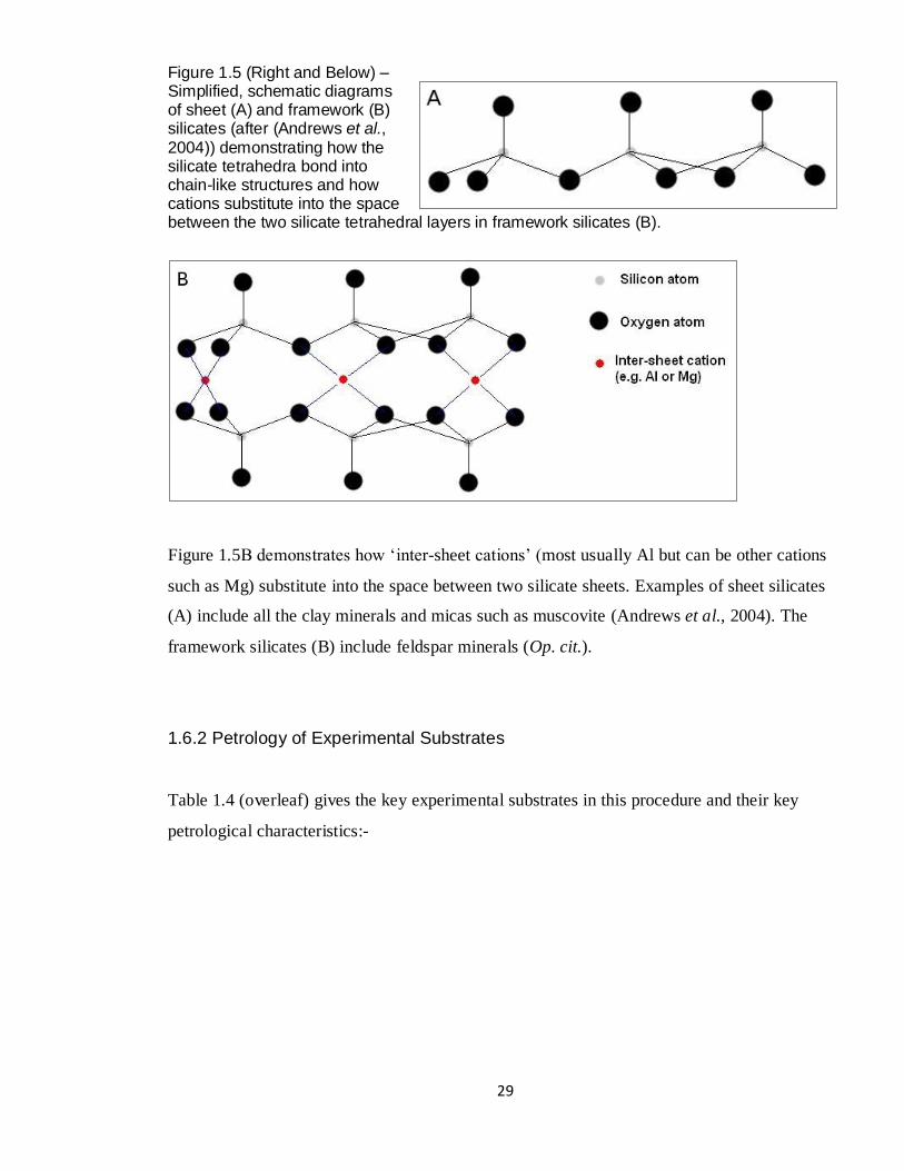
Figure 1.5 (Right and Below) – Simplified, schematic diagrams of sheet (A) and framework (B) silicates (after (Andrews et al., 2004)) demonstrating how the silicate tetrahedra bond into chain-like structures and how cations substitute into the space between the two silicate tetrahedral layers in framework silicates (B).
Figure 1.5B demonstrates how „inter-sheet cations‟ (most usually Al but can be other cations
such as Mg) substitute into the space between two silicate sheets. Examples of sheet silicates
(A) include all the clay minerals and micas such as muscovite (Andrews et al., 2004). The
framework silicates (B) include feldspar minerals (Op. cit.).
1.6.2 Petrology of Experimental Substrates
Table 1.4 (overleaf) gives the key experimental substrates in this procedure and their key
petrological characteristics:-

30
Substrate
Name
Description
Andesite
Andesite is an igneous, volcanic rock containing a large proportion of
feldspar (an aluminosilicate mineral) (Mackenzie & Adams, 1994).
Granite
Granite is an igneous rock containing ~70% Quartz (SiO2) by mass of rock
(Blatt et al., 2006). Also contains feldspar (Mackenzie & Adams, 1994).
Vermiculite
Vermiculite is a framework, exfoliated aluminosilicate mineral that is
chemically similar to smectite clay (Andrews et al. (2004); Deer et al.
(1966)). It is formed by alteration of the mineral biotite or volcanic minerals
(e.g. chlorites and hornblende) by either weathering or hydrothermal action
(Deer et al., 1966). Mg is the main inter-sheet cation (Op. cit.).
Clay
Clay minerals are sheet silicates formed by the weathering of other rocks
(Andrews et al., 2004). The chemical composition of clays varies
depending on the extent of alteration (Deer et al., 1966).
Basalt
Basalt is a fine-grained, plagioclase-rich, igneous rock (Mackenzie &
Adams, 1994).
Chlorite Chlorite has a layered structure similar to mica in which Mg, Al and Fe are
susceptible to isomorphic substitution (Deer et al., 1966).
Table 1.4 – The experimental substrates and their key petrological properties.
1.7 Measuring Weathering
Weathering cannot be directly measured, therefore other parameters have to be measured that
are assumed to be proportional to weathering. Previous studies have used the thickness of
secondary material formed as a result of weathering (the „weathering crust‟) to calculate
weathering rates (e.g. Jackson & Keller (1970)). Some studies (e.g. Jackson & Keller (1970);
Ford Cochran & Berner (1996) etc.) have used in situ ion microprobe analysis to analyse rock
surfaces colonised by biota and un-colonised rock to measure chemical differences indicative
of weathering. Other studies (e.g. Moulton & Berner (1998); Aghamiri & Schwartzman
(2002) etc.) exploit the fact that when ions are weathered they tend to enter the aqueous phase.
This aqueous solution can be used as a matrix for chemical analysis, hence weathering can be

31
measured. Moulton & Berner (1998) describe “The flux of dissolved… cations, anions, and
silica… (as a) sensitive indicator of the extent of silicate rock weathering”.
All of the studies previously mentioned in this section are „mesocosm experiments‟, that is to
say: experiments that study real-world processes on a small-scale in-situ. This thesis reports
the results from a „microcosm study‟, meaning that experiments into real-word processes will
be conducted on a very small scale in-vitro (in sterile conditions in the laboratory). There are
two main benefits to microcosm experiments over mesocosm experiments:-
1. It is far simpler to control experimental variables (e.g. sterility, heating and lighting
regimes) in a laboratory setting.
2. Microcosm experiments can be repeated many times at minimal cost compared with
mesocosm studies (which tend to involve higher cost and the much greater logistical
difficulties associated with work in the field).
Care must be taken with respect to point 1; over-controlling environmental variables can make
experiments innately un-realistic and can have an adverse effect on experimental results (see
White & Brantley (2003) for a discussion of this effect in a geochemical context).
1.8 Summary
Drawing on the commonality of a number of different studies into the potential causes of the
Ordovician glaciation and the results of some very recent palynolological studies into
bryophyte evolution and distribution, and the synergy between stratigraphic and palynological
data e.g. the fact that the oldest record of bryophyte-like cryptospores (Steemans et al., 2009)
coincides with the first („Darriwilian‟) δ13
C excursion, a very interesting hypothesis emerges.
If this study proves that bryophytes significantly increase the biotic enhancement of mineral
weathering it will lend weight to hypotheses regarding increased weathering as the „smoking
gun‟ of the Ordovician glaciation (Kump et al. (1999); Sheehan (2001); Saltzman & Young
(2005)) and will establish a new hypothesis that early bryophyte-like organisms were
responsible for this increased weathering.

32
A literature search using ISI Web of Knowledge, Web of Science4 and Google Scholar
5
revealed no precedent for microcosm studies into the biotic enhancement of mineral
weathering by moss. The literature search was conducted on 2/1/2010 using the search terms
„microcosm AND moss AND weathering‟, and the only similar study was Baars et al. (2008)
which concentrated on the effects of carbon dioxide saturation on the soil zone.
The primary aim of this study will therefore be to measure the biotic enhancement of mineral
weathering on different rocks and minerals in a microcosm study. The resulting data will be
used to validate or falsify the null and alternative hypothesis outlined in the following section.
Figure 1.6 (below) shows photographs of a microcosm.
Figure 1.6 - Side and plan views of a Basalt microcosm (after a weathering period of 138 days).
4 http://apps.isiknowledge.com 5 http://scholar.google.co.uk

33
1.9 Conceptual Framework
If Wabiotic = abiotic weathering measurable by the method to be employed in this study,
Wbiotic= biotic weathering measurable by the method and Wmoss = the amounts of analytes
resulting from moss recovered from moss colonised („mossed‟) microcosms, the following can
be deduced:-
Equation 1.5 – Total weathering must equal the sum of abiotic weathering, biotic weathering and weathered ions uptaken by the moss.
For the purposes of this study the amounts of analytes contained within the aqueous solution
removed from control microcosms after correction for the relevant blanks will be assumed to
represent abiotic weathering (henceforth referred to as Wa). The amounts of analytes contained
within the aqueous solution resulting from mossed microcosms will be taken to represent total
aqueous weathering, after correction for the relevant blanks (i.e. both abiotic and biotic
aqueous weathering) and will henceforth be referred to as Wb. After correction for the relevant
blanks Wmoss must represent the amount of analyte resulting from weathering that is taken up
by the moss. Given that Wb actually represents both abiotic and biotic weathering Equation 1.5
can be reformed thus:-
Equation 1.6 – Actual equation for total weathering (W tot) inferred from the amounts of analytes contained within biotic (mossed) microcosm components.

34
Net biotic weathering (Wnetbio), i.e. the additional weathering occurring in a microcosm as a
result of biota being present, can be regarded as being:-
Equation 1.7 – Calculation for net biotic weathering (W netbio).
The biotic enhancement of weathering (Ψ) can therefore be defined as a factor of net biotic
weathering divided by abiotic weathering thus:-
Equation 1.8 – The Biotic Enhancement of Weathering calculation.
Where Ψ ≤1 there is no measurable biotic enhancement of weathering, where Ψ>1 there is
biotic enhancement of weathering, measurable using the methods to be employed in this study.
Below are a null (H0) and an alternative (H1) hypothesis related to the biotic enhancement of
weathering:-
H0 = Wtot for analyte x on substrate y is not statistically greater than Wa for analyte x on
substrate y at the P<0.05 level. Analyte x is not biotically enhanced on substrate y.
H1 = Wtot for analyte x on substrate y is statistically greater than Wa for analyte x on substrate
y at the P<0.05 level. Analyte x is biotically enhanced on substrate y.

35
2: Experimental Methods
2.1 Overall Approach
The work reported in this thesis used an approach similar to Moulton & Berner (1998);
Aghamiri & Schwartzman (2002) and others in that it exploited the fact that the products of
weathering are removed from a rock‟s surface by water (in the natural environment this water
takes the form of precipitation or the flow of rivers), the polar nature of the water molecule
attracting weathered ions.
The experimental procedure itself was a microcosm study: the microcosms consisted of plastic
jars into which a small amount of rock or mineral substrate was placed. Moss cells suspended
in a constant volume of water were added to half of these microcosms and the other half had
the same volume of water added and served as controls. Excess concentration of an analyte in
the moss-colonised microcosms above the concentration present in control microcosms (after
corrections for blanks etc.) can be assumed to result directly as a consequence of the moss
weathering the rock (provided the procedure is undertaken correctly).

36
Figure 2.1 – Summary flow chart of key stages in the experimental procedure from the culturing of the moss on compost plugs (‘jiffys’) through to the weathering period of the microcosms with the section number where the process is discussed fully noted. An asterisk (*) indicates that this part of the procedure was conducted using sterile technique (see §2.9).
As a number of new methods were developed during the experimental procedure a number of
new terms were devised. Terms were also devised in order to adequately explain a concept as
succinctly as possible. Devised terms are explained when they first appear.

37
2.2 Substrate and Microcosm Preparation
Table 2.1 (below) gives details of the experimental substrates, their sources and details of how
substrate petrology was determined:-
Experimental
Substrate
Source and Identification
Andesite
Supplied by: John Wainwright and Co. Ltd., Moons Hill Quarry,
Radstock, UK. XRF analysed.
Granite
Bradstone Silver Granite supplied by: Aggregate Industries PLC,
Hulland Ward, Ashbourne, Derbyshire, DE6 3ET, UK. Granite quarried
in Penryn, Cornwall, UK. XRF analysed.
Vermiculite Supplied by: Sinclair, Lincoln, UK. XRF analysed.
Clay
Of unknown origin. Supplied by a horticultural products company. No
XRF analysis, examined using naked eye.
Basalt
A limited amount (one rock), collected in Indonesia. No XRF analysis,
examined using naked eye.
Chlorite Collected in the Dunmail Raise area of the Lake District National Park,
England (OS Grid Ref. NY334073). XRF analysed.
Table 2.1 – The experimental substrates, their source and mode of identification. Andesite and granite formed the key experimental substrates.

38
Figure 2.2 (Left) – Flow chart depicting the main stages in the substrate and microcosm preparation procedures. An asterisk (*) indicates that this part of the procedure was conducted using sterile technique (see §2.9).
Figure 2.2 (above) summarises the key stages in the substrate and microcosm preparation
stages: basalt and chlorite rocks were cut into rectangular prisms ~20mm x ~10mm x ~5mm
using a diamond tipped saw. Granite and vermiculite were simply graded using sieves
decreasing in aperture size from 4mm at the top to 1mm at the bottom of the column. This
column of sieves was placed into an Endecotts8 test sieve shaker, and the substrate placed into
the sieve with the largest aperture diameter at the top of the stack. The sieve shaker was then
timed to shake for a period of 10 minutes. After 10 minutes the fraction yielding the most
material was retained (>2.8mm for granite, >1.4mm for vermiculite), the remaining material
8 Endecotts Ltd., 9 Lombard Road, London, SW19 3TZ, UK.

39
was discarded. After 10 minutes the clasts were well sorted. Only a limited number of
experiments were conducted on clay, basalt and the chlorite rock due to a shortage of available
material.
After grading/cutting the material was washed three times with ultra pure water (henceforth
referred to as „upH2O‟) in order to remove any nutrients which may have been adsorbed to the
surface of the substrate (the full washing protocol can be found in Appendix i.ii.i and an
analysis of the washes can be found in Appendix ii.iii). Ideally, the only nutrients that should
be present in the microcosm system are those within the substrate itself and those within the
solutions added to microcosms in order to conduct the experiment. By sampling these
fractions the budget can be closed, therefore any nutrients contained within the moss tissue
(after correction for that contained within solutions added to the microcosms) must result as a
consequence of weathering.
The substrate was then heat sterilised in order to kill any biota capable of weathering the
substrate (e.g. fungi, bacteria). Substrates were sterilised in a 180°C oven for a period of not
less than 16 hours and not more than 24 hours. Heat sterilising had the added effect of killing
any biota that may have been present, whilst also driving off all water ensuring that dry
substrate was used to prepare the microcosms. Substrates were frequently stored for prolonged
periods (sometimes as long as 3 months) in between uses, material was stored in glass beakers
covered with aluminium foil and was heat sterilised again prior to re-use as a precaution
against contamination by biota.
In early pilot experiments (not analysed) the substrate was autoclaved instead of heat
sterilised, resulting in the substrate becoming highly saturated with water. This was not ideal
because there was no way of ensuring that the water was absorbed homogeneously throughout
the substrate, and such varying dilution rates could adversely affect the data relating to ionic
dissolution into the aqueous phase obtained at the end of the experiment. Samples of both
washed and unwashed rock/mineral were taken for solid phase XRF analysis in order to
determine the chemical composition of the substrate. For the substrates consisting of large
clasts (granite, chlorite and basalt) approximately six clasts were added to a plastic screw-top
jar9 using sterilised forceps. The masses of granite added to the microcosms in the 30/4/08,
9 Sterilin Ltd., Angel Lane, Bargoed, Caerphilly, CF81 9FW.

40
2/9/08 and 11/9/08 granite experiments were recorded, the mean mass of granite added in
these three experiments being 23.66g (±4.70). Enough material was added to cover the bottom
of the jar, as far as possible. For the finer-grained substrates (andesite, vermiculite and clay) an
exemplar jar was set up with material added to a depth of ~6.5mm. This depth of material
equated to a number of heaped spoonfuls and this number of spoonfuls was added to
subsequent pots using a sterilised metal spoon.
Control microcosms were prepared by adding 3ml of filtrate using a 5ml air displacement
pipette. The lids to the jars when then screwed down under a laminar flow hood (all pipette
tips were autoclaved prior to use). Mossed microcosms were prepared by adding a total of 3ml
of moss inoculum in 2x1.5ml increments in order to promote horizontal growth across the
surface, rather than „bunching up‟ the moss into one mass (for details on how moss inoculum
and filtrate were prepared see §2.11). Tips were specially prepared for this purpose by cutting
off the narrow ends using a razor blade (as the moss inoculum tended to get stuck). Care was
taken to ensure that the same length was cut-off each tip as this could affect the volume
pipetted. Moss rapidly settles at the bottom of a container, to avoid this; the inoculum was
swirled gently by hand before the suspension was drawn into the pipette tip. The lids to the
jars were then screwed down as previously described.
2.3 Microcosm Treatment
Jars were placed in a random fashion to avoid artefacts due to a lack of spatial heterogeneity
within the growth room. Microcosms were grown for at least 90 days, except in cases where
moss began to die sooner than this, in which case the microcosms were sampled as soon as
possible after death occurred. Dead moss was observed to turn a shade of yellow/brown or a
translucent, bleached colour. The mean weathering period across all experiments was 112
days. Within 24-72 hours of inoculation water condenses into droplets on the wall of the
sterile jar. On sampling the microcosms a very small volume of water can also be found
condensed on the lid. Table 2.2 (overleaf) summarises all of the microcosm experiments and
their growth periods.

41
Substrate Sample size (n)
Date microcosms were initiated
Date microcosms were sampled
Weathering period (days)
Clay Mossed = 6†, Control = 6†.
18/12/07 19/2/08 63
Vermiculite Mossed = 6†, Control = 6†.
18/12/07 19/2/08 63
Vermiculite Mossed = 20, Control = 20.
14/2/08 24/7/08 161
Vermiculite Mossed = 17, Control = 17.
17/2/09 22/7/09 155
Granite Mossed = 9, Control = 10.
30/4/08 18/8/08 110
Granite Mossed = 7, Control = 10
24/6/08‡ 9/11/08 138
Granite Mossed = 7†, Control = 10†.
15/8/08 15/12/08 121
Granite Mossed = 15, Control = 14.
2/9/08 22/12/08 111
Granite Mossed = 14, Control = 14.
19/12/08 29/4/09 100
Granite Mossed = 14, Control = 14.
12/1/09 10/6/09 149
Granite Mossed = 14, Control = 15.
30/7/09‡ 18/9/09 50*
Chlorite Mossed = 7, Control = 7.
24/6/08‡ 4/9/08 72*
Chlorite Mossed = 7, Control = 7.
15/8/08 15/12/08 121
Basalt Mossed = 7†, Control = 5.
24/6/08‡ 9/11/08 138
Andesite Mossed = 7, Control = 7.
28/11/08 2/2/09 66*
Andesite Mossed = 11, Control = 9.
2/12/08 22/6/09 202
Andesite Mossed = 24, Control = 21.
25/1/09 2/7/09 158
No substrate, Inoculum only
Mossed = 14, Control = 0.
30/7/09‡ 18/9/09 50*
Table 2.2 – The microcosm experiments arranged by substrate and then in chronological order. Proof of concept/method development experiments are italicised. n = n used to form data in §4 or Appendix iv (with microcosms used for photography, spilled samples etc. excluded) unless otherwise stated with ‘†’ symbol. Shaded experiments were initiated by Nuno Pires and sampled by the author. † n = total n of microcosms initiated. ‡ Same inoculum used across all substrates for that date. * Microcosms sampled <90 days because moss was dying.

42
2.4 Sampling the Moss Biomass from Microcosms
Figure 2.3 (Left) – Flow chart of the main stages in the microcosm sample preparation and sample analysis procedures All stages in this flow chart were conducted using a clean but not sterile technique. For details on sample analysis see §3.
The microcosm sampling procedure was conducted on an open lab bench maintaining a clean
but not sterile technique. In the case of mossed microcosms: the moss was removed from the
microcosms using forceps and placed on filter paper. A 100ml plastic beaker was placed over
the moss in order to minimise contamination. The moss was left to air dry for approximately
48 hours before being transferred to a new, pre-weighed 50ml centrifuge tube10
(early pilot
studies dried the moss in porcelain crucibles within a 55°C oven for 16 hours, but it was found
10 Manufactured by: Corning Inc., One Riverfront Plaza, Corning, NY 14831, USA.
43
that a large mass of recovered moss was lost due to the moss adhering tightly to the crucible).
The tube was then weighed again once the moss had been placed into the centrifuge tube
(weighing was conducted using a balance with an accuracy of ±0.0001g) in order to give a
mass of moss recovered from each mossed microcosm. The centrifuge tubes with moss were
then stored at <4°C prior to wet oxidation.
It is important to note that in the large clast substrates (e.g. granite); some moss tissue
remained in the microcosm after forcep removal (the mass of moss remaining in the
microcosm being a small fraction of that which was recovered, one-tenth being a liberal
estimate). For the fine grained substrates; it was very difficult to remove the moss biomass as
the rhizines formed an extensive network between the small grains, causing moss and
substrate to bind tightly together. This was especially the case for vermiculite microcosms due
to the substrate‟s highly exfoliated morphology. Both the moss biomass from vermiculite (see
Figure 2.4, below) and andesite microcosms were cleaned by placing the sample under a
stereo microscope and cleaning with two forceps.
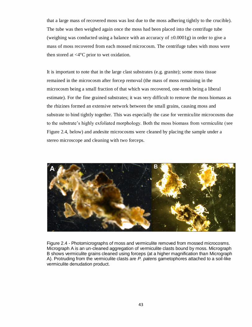
Figure 2.4 - Photomicrographs of moss and vermiculite removed from mossed microcosms. Micrograph A is an un-cleaned aggregation of vermiculite clasts bound by moss. Micrograph B shows vermiculite grains cleaned using forceps (at a higher magnification than Micrograph A). Protruding from the vermiculite clasts are P. patens gametophores attached to a soil-like vermiculite denudation product.

44
2.5 The Biomass Oxidation Method
2.5.1 Rationale
In order to determine the amounts of analyte within moss removed from microcosms and
aliquots of the moss inoculum two key things were necessary:-
1: A method had to be found (or developed) to dissolve the nutrient and metal ions contained
within the moss biomass as completely as possible.
2: The nutrient and metal ions within solutions then had to be measured using standard
analytical methods available locally.
A literature search highlighted various methods employing concentrated acids and
temperatures >100ºC (e.g. Sapkota et al. (2005) and Sucharova & Suchara (2006)). These
methods were discounted because the risks were deemed to be unacceptable and because
necessary equipment and facilities (e.g. a microwave autoclave and the facilities to handle
strong acids) were not available locally and would have required highly specialised training.
Therefore a new method had to be developed. Pilot oxidation experiments were conducted
using tissue from the seed-plant Arabidopsis thaliana (for details of these experiments see
Appendix i.i.i).

45
2.5.2 Methodology
Figure 2.5 (Left) - Flow chart depicting the Biomass Oxidation Method. All stages in this flow chart were conducted using a clean but not sterile technique. Heating of acids was conducted in a fume cupboard and appropriate Personal Protective Equipment was worn at all times.
A heating block was set to 70°C and a centrifuge tube
containing 20ml water and a thermometer was placed
into it. Once the water reached 70°C (±5°C) the tubes
containing moss and acid were heated for 30 minutes.
Caps were kept loose for most of the procedure in order
to allow oxygen gas formed as the Hydrogen Peroxide
degrades to escape (H2O2(aq.) → O2(g)). Periodically the
tubes were sealed and shaken briskly. The moss/acid
mixtures were not allowed to exceed 75°C as at this
temperature the solutions start to become unstable due to
the more rapid evolution of oxygen gas.
After 30 minutes of heating the tubes were allowed to
cool with the lids on top, outside of the heat block (but within the fume cupboard). Once the
solutions had cooled to room temperature they were filtered using 0.2μm Sartorius Minisart®
cellulose acetate syringe tip filters11
(NB all filters used throughout the experimental
procedure are of cellulose acetate type). The resulting samples were then stored at <4°C. The
tubes should not be fully sealed but kept a ¼ turn loose as a precaution in case any more
oxygen gas evolves
Early inoculum blanks (up to and including the 25/6/08 inoculum blanks) were frozen whilst
the Biomass Oxidation Method was developed. All other inoculum samples were stored in a
<4°C cold room for no more than two months. It is unlikely that the polypropylene plastic
centrifuge tubes liberated contaminants into the oxidising solution at room temperature;
11 Sartorius Stedim Biotech. GmbH, 37070 Goettingen, Germany.

46
however the author was concerned that the high temperatures encountered in the heating block
may cause contaminants to be leached into solution from the centrifuge tube walls. Five tubes
containing 20ml of upH2O were therefore heated for 30 minutes with shaking in order to
replicate the conditions encountered by moss samples during oxidations. This upH2O was then
analysed and the resulting data are given in Appendix ii.iv.
2.6 Sampling the Aqueous Solution from Microcosms
2.6.1 Introduction
Once the moss was removed from the mossed microcosms both mossed and control
microcosms could be treated in the same manner and the resulting aqueous solution from all
microcosms could be sampled.
Three different methods were used for microcosm water sampling during the method
development phase before a suitable method was found. The method applied to each set of
microcosm experiments is depicted in the table below:-
Microcosm water sampling method Experiment/s method was applied to
1 October 2007 – Vermiculite and Clay
2 14/2/08 Vermiculite
3 30/4/08 Granite and all subsequent
Table 2.3 – The microcosm water sampling methods.
The changes in dilution factor brought about by these three different sampling methods have
been corrected for during data analysis. Sampling Method 3 addressed the problem that the
aqueous fraction from the microcosms was highly diluted by added upH2O (by a factor of 23
and 18.6 for methods 1 and 2 respectively). The dilution factor for method 3 is 3.3.

47
2.6.2 Methodology
Fifteen microcosms at a time were placed onto a Luckham 4-RT rocking table12
(see Figure
2.3, p42). The rocking table was switched on and 5ml of upH2O was pipetted into the first
microcosm, simultaneously a timer was started. Every minute 5ml of upH2O was pipetted into
the next microcosm in the sequence. After 15 mins had elapsed an extra 5ml of upH2O was
added to the first microcosm in the sequence and this process continued.
After 30 mins of elapsed time, 10ml of solution was drawn off of the first microcosm in two
pipettings and placed into a new centrifuge tube. This process was continued every minute
until 10ml of solution was drawn off of each microcosm. The 10ml resulting solution was then
filtered using new 0.2µm filters into another centrifuge tube.
2.7 Photography
Plan and side photographs of the microcosms were taken in a studio, usually against a black
background. Beads of condensation on the plastic jar sides frequently obscured the substrate
and/or the moss, therefore swabs and a hair dryer had to be used to remove the condensation
before photographing. Because of this treatment the aqueous solutions and moss from
photographed microcosms were not sampled. Photographs can be seen in §4.3/4.4.
2.8 Cleaning Techniques
Two grades of ultra pure water were used in the procedure; some provided by an ELGA13
Purelab®
Mk.1 Option unit and some provided by the newer ELGA Purelab®
Mk. 2 Genetic
Ultra unit. Both of the „ELGA‟ units intake reverse osmosis filtered, de-ionised water
(henceforth known as dH2O), pass it through a primary filter and then a secondary „polishing‟
filter before treating the water with ultra-violet radiation to kill any biota. Water generated by
the Mk. 1 unit had a resistivity of 15MΩ (pH 5.37), water generated by the Mk. 2 unit had a
resistivity of 18MΩ (pH 5.13). Resistivity (MΩ) is inversely proportional to ionic
12 Luckham Ltd., Burgess Hill, UK. 13 ELGA Process Water, Marlow International, Park Way, Marlow, Bucks, SL7 1YL.

48
contamination (see Appendix ii.i.i). Unless otherwise stated „upH2O‟ refers to the 18MΩ
water from the Mk. 2 unit. Ultra-Pure Water was stored in an aspirator which had been rinsed
with a 5% solution of Decon 90®15
(as per Spokes et al. (2000)) before rinsing with dH2O until
no foam was formed. A final rinse with upH2O was then given.
Initially blanks of the ultra pure water were taken only when the aspirator was re-filled and
sporadically between fillings. After 9/11/2008 blanks were taken on each day that a procedure
was conducted using upH2O. upH2O blanks were taken from the beaker used to store the
solution on the lab bench. Blanks were taken before experimental work commenced, by
pouring upH2O from the container directly into new centrifuge tubes which were then sealed
prior to analysis by Inductively Coupled Plasma – Atomic Emission Spectrometry (ICP-AES,
see §3.1/3.2).
2.9 Preparation of Cultures and Growth Conditions
Culturing and growth of the moss, preparation of the moss inoculum and preparation of the
microcosms were all conducted using sterile technique (Taylor et al., 1997). All of the
processes were conducted under a laminar flow hood, the surfaces of which were pre-cleaned
with a 70% ethanol solution. All metal instruments were treated with 70% ethanol solution
and heated in a flame.
Where possible items of equipment (petri dishes, centrifuge tubes, serological pipette tips etc.)
were purchased from suppliers who assured sterility by gamma irradiation sterilisation and
hermetic sealing. Where items could not be purchased sterile (Gilson-type pipette tips,
cellulose discs etc.) items were autoclaved using an Astell Scientific Swiftlock 2000/9016
steam generator set to a programme of 121°C, for 20 minutes. Indicator tape was used to
ensure that all autoclaved items had been exposed to steam. Sterile water was used extensively
throughout the experimental procedure, which is upH2O that is subsequently autoclaved in
bijou jars (a small glass jar with a screw-top lid). Chemicals used in all parts of the procedure
were of analytical reagent grade quality. Appendix ii.i.ii shows that there is less Al and Fe
15 Decon Laboratories Ltd., Conway Street, Hove, East Sussex, BN3 3LY, UK. 16 Astell Scientific Ltd, Sidcup, Kent, DA14 5DT, UK.

49
contamination in sterile water relative to 18MΩ (insignificant; 1σ error bars overlap), but
significantly more Si contamination in the sterile water (possibly due to the fact that sterile
water is autoclaved at high temperature and pressure in a silica glass bijou jar).
A clean technique was maintained by decontaminating lab-ware by Decon rinsing (as
previously described) and then wrapping items with cling film, or sealing them at the top with
cling film (e.g. beakers and measuring cylinders). Sterile technique had to take precedence
over clean technique as it was imperative that the inoculum did not become infected with
fungi as this could cause morbidity in the moss, and also introduce weathering artefacts due to
acid exudates from the fungal hyphae (roots) (Hoffland et al., 2004).
Moss cultures and microcosms were stored in a growth room. The growth room was
maintained at 25ºC with a photoperiod of 16 hours light and 8 hours darkness, which is
standard conditions for the culture of P. patens (Marienfeld et al., 1989). The light was
provided by two fluorescent tubes mounted above the shelves on which the cultures or
microcosms were placed. Light flux and quality were measured using a Macam L300
Photometer18
. Both fluorescent tubes radiated a total integrated light flux of 120µmol m-2
s1
(120µmol photons m-2
s1) or 25.2W m
-2.
18 Macam Radiometrics, 10 Kelvin Square, Livingston, Scotland.
50
2.10 Culturing of Moss Tissue
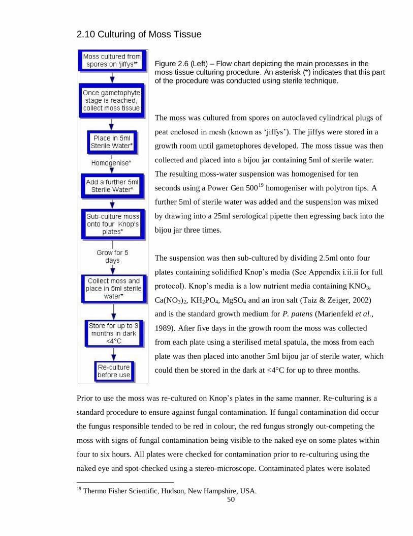
Figure 2.6 (Left) – Flow chart depicting the main processes in the moss tissue culturing procedure. An asterisk (*) indicates that this part of the procedure was conducted using sterile technique.
The moss was cultured from spores on autoclaved cylindrical plugs of
peat enclosed in mesh (known as „jiffys‟). The jiffys were stored in a
growth room until gametophores developed. The moss tissue was then
collected and placed into a bijou jar containing 5ml of sterile water.
The resulting moss-water suspension was homogenised for ten
seconds using a Power Gen 50019
homogeniser with polytron tips. A
further 5ml of sterile water was added and the suspension was mixed
by drawing into a 25ml serological pipette then egressing back into the
bijou jar three times.
The suspension was then sub-cultured by dividing 2.5ml onto four
plates containing solidified Knop‟s media (See Appendix i.ii.ii for full
protocol). Knop‟s media is a low nutrient media containing KNO3,
Ca(NO3)2, KH2PO4, MgSO4 and an iron salt (Taiz & Zeiger, 2002)
and is the standard growth medium for P. patens (Marienfeld et al.,
1989). After five days in the growth room the moss was collected
from each plate using a sterilised metal spatula, the moss from each
plate was then placed into another 5ml bijou jar of sterile water, which
could then be stored in the dark at <4°C for up to three months.
Prior to use the moss was re-cultured on Knop‟s plates in the same manner. Re-culturing is a
standard procedure to ensure against fungal contamination. If fungal contamination did occur
the fungus responsible tended to be red in colour, the red fungus strongly out-competing the
moss with signs of fungal contamination being visible to the naked eye on some plates within
four to six hours. All plates were checked for contamination prior to re-culturing using the
naked eye and spot-checked using a stereo-microscope. Contaminated plates were isolated
19 Thermo Fisher Scientific, Hudson, New Hampshire, USA.

51
from uncontaminated plates and „killed‟ by autoclaving. Great care was taken not to use
fungal contaminated plates for inoculum preparation; as a result only one microcosm across all
experiments became contaminated with the red fungus (a microcosm in the 2/9/08 granite
experiment which was excluded from the dataset).
After five days growth on Knop‟s plates the moss was removed, added to 5ml sterile water
and homogenised. A further 5ml of sterile water was then added and the solution mixed in a
pipette. The moss suspensions were then ready for use in inoculum preparation.
2.11 Moss Inoculum and Filtrate Preparation
Figure 2.7 (Left) – Flow chart depicting the main stages in the moss inoculum and filtrate preparation procedures. An asterisk (*) indicates that this part of the procedure was conducted using sterile technique.
Using a 25ml pipette the moss suspensions were
transferred to a sterile 250ml glass conical flask:
sterile water was then added to the 250ml line and
the solution was mixed using a pipette. Excess
aqueous solution was then pipetted off until
~120ml of moss/water suspension remained
(forming the first wash of the moss). The process
was then repeated, giving a second wash of the
moss with sterile water.
Sterile upH2O was then added to the 250ml line
(this was upH2O that had been 0.2μm filtered into
a separate sterile 250ml conical flask to exclude
any biota that may be present). The suspension
was then mixed and the excess aqueous solution
was pipetted off and placed into a separate conical

52
flask until 80-120ml of concentrated moss suspension remained. The remaining concentrated
moss suspension formed the moss inoculum and the excess aqueous solution (essentially the
third wash of the moss inoculum) was filtered using a 0.2μm filter and is known as the
„filtrate‟.
The volume of moss inoculum was measured before and after filtering the aqueous portion off.
12 inoculum pseudo-replicates were measured from five different inoculum preparations (n ≥2
for each inoculum preparation). The mean volume of the inoculum before filtration was
19.0ml and the mean volume afterwards was 14.1ml indicating that 74.4% (±8.6%) of the
moss inoculum was in the form of water. The washing procedure used to clean the moss and
prepare it for inoculation and to prepare the filtrate is highly efficient at removing adsorbed
contaminants and ensuring that the moss and filtrate are as clean as possible whilst
maintaining the viability of moss as a living organism. Appendix ii.ii consists of graphs
showing the levels of contamination present at the different preparation stages of the 29/7/09
inoculum.

53
3: Analytical Methods
3.1 Introduction
Three different analytical methods were used within the experimental procedure: an
Inductively Coupled Plasma - Atomic Emission Spectrometer (henceforth known as the „ICP-
AES‟ or „ICP‟) and a Nutrient Auto Analyser („NAA‟) for aqueous phase analysis of the
resulting solutions from microcosms and oxidised moss samples. An X-Ray Fluorescence
Spectrometer („XRF‟) was used for solid phase analysis of the rock and mineral substrates.
ICP spectroscopy has been used in previous studies into the biotic enhancement of weathering
such as Moulton & Berner (1998) and Aghamiri & Schwartzman (2002).
3.2 Sample Preparation
If not already done so samples were filtered using 0.2µm filters in order to prevent damage to
the ICP‟s internal mechanisms (glassware such as the nebuliser is particularly susceptible to
damage from fine solids) (Lajunen & Peramaki, 2004). The samples were then split into two
aliquots: one for ICP analysis and another for Nutrient Auto-Analysis (NAA) and as a backup
ICP sample in case of instrumental failure or other loss. A separate syringe and filter were
used for each sample to prevent contamination (except pseudo-replicated samples and the
substrate washes). In the case of the substrate washes (particularly for the initial washes of the
fine-grained substrates) the filters clogged very quickly, and it was not uncommon to have to
use three filters on one 50ml sample. Samples were then stored at <4°C. Samples were not
routinely frozen (as suggested by Parsons et al. (1984) as previous experiments have shown
that 15ml and 50ml centrifuge tubes manufactured by two different companies routinely crack
at -20°C, resulting in sample loss (Crouch, 2007). Parsons et al. (1984) advise storing 50ml of
sample in a 125ml screw-cap polyethylene bottle at -20°C if analysis cannot be conducted
immediately, this reference was only discovered after conducting the experimental procedure,
and in future this approach should be adopted where possible.
A 10% hydrochloric acid/upH2O solution was added to ICP aliquots and blanks in a volume
ratio of 1:10 hydrochloric acid:sample in order to desorb any metal ions which may have

54
adsorbed to the side of the centrifuge tubes (Lajunen & Peramaki, 2004). The 10%
hydrochloric acid (henceforth known as the „desorbing agent‟) was added and the samples
lightly shaken immediately prior to an ICP run. Blanks of the desorbing agent were also taken
at this point. This method assured (as far as possible) that contamination from the desorbing
agent remained uniform across all samples in a run. Early desorbing agent (1/2/08 batch, used
to desorb ICP runs 1-4 inclusive) was stored in a glass container and was subsequently found
to be substantially contaminated with Al, Ca, K, Na and (particularly) Si. Contamination in
this batch was 1-2 magnitude greater for these analytes than subsequent batches which were
stored in polypropylene. Contamination of solutions stored in glassware by the glass itself is a
known phenomenon (especially Si dissolution from glassware, even by relatively weak acids)
(Liss & Spencer (1969) and Zhang et al. (1999)). The experimental implications for the
contamination in this batch was that if the weathering signal was smaller than the
contamination from glassware the weathering signal could be „drowned out‟ by the
contamination signal.
The only ICP samples which were not desorbed in the aforementioned manner were the moss
oxidations as these samples already contain 2ml of their 4ml ICP volume as nitric acid, which
is also a candidate desorbing agent (Lajunen & Peramaki, 2004). Furthermore: the reaction
between hydrochloric acid and nitric acid could promote the evolution of toxic chlorine gas.

55
3.3 ICP-AES Analysis
3.3.1 Introduction
A Varian† Vista Pro Inductively Coupled Plasma, Optical Emission Spectrometer was used to
determine the concentrations of the following analytes:-
ICP Analyte Symbol Emission Wavelength λ (nm)
Aluminium Al 396.152 Calcium Ca 422.673
Iron Fe 259.940 Potassium K 766.491
Magnesium Mg 285.213
Sodium Na 589.592 Silicon Si 251.611
Table 3.1 – Table showing ICP-AES analytes and the emission wavelengths used to measure the concentration of those analytes (NB different emission wavelengths can be used to avoid spectral-overlap interference which could lead to erroneous concentrations being recorded for an analyte (Lajunen & Peramaki, 2004).
The ICP was fitted with a Varian SPS 5 sample preparation system for automated sampling.
The concentration of samples was recorded automatically on a linked PC using Varian Vista
Pro software. These data were then exported into Microsoft Excel.
3.3.2 Calibration
The ICP was calibrated using five standards. Two working standards were prepared using
SpexCertiPrep20®
ClaritasPPT®
certified reference standards and ultra-pure (18MΩ) water
supplied via a Milli-QTM Advantage A10 system
21. One working standard was a mixed
elemental standard containing Al, Ca, Fe, K, Mg and Na and the other was a single elemental
standard containing Si. This working standard was used to prepare five calibration standards,
The concentrations of which are given in Table 3.2 (overleaf).
† Varian Inc., Palo Alto, California, USA. 20 SpexCentriPrep Inc., 203 Norcross Avenue, Meutchen, NJ08840, USA. 21 Millipore (UK) Ltd., 3-5 The Courtyards, Hatters Lane, Watford, Herts., WD18 8YH, UK.

56
[Al] [Ca] [Fe] [K] [Mg] [Na] [Si]
Standard 1 0.7412 99.8004 0.3581 25.5766 41.1438 130.4928 7.1211
Standard 2 1.4825 199.6008 0.7162 51.1531 82.2876 260.9856 14.2422
Standard 3 2.2237 299.4012 1.0744 76.7297 123.4314 391.4785 21.3633
Standard 4 2.9650 399.2016 1.4325 102.3062 164.5752 521.9713 28.4844
Standard 5 3.7062 499.0020 1.7906 127.8828 205.7190 652.4641 35.6056
Table 3.2 – The ICP-AES standards (figures in μmol l-1). Standards were prepared in mg l-1, hence the non-round numbers.
Table 3.3 and Figure 3.1 (below and overleaf) give an example of the calibration data obtained
by the ICP, in this case; the calibration for Al in Round 10:-
Standard
Concentration
ICP Calculated
Concentration
Error
Blank 0.000000 0.000000 0.000
1 0.020000 0.019228 -0.001
2 0.040000 0.039002 -0.001
3 0.060000 0.059160 -0.001
4 0.080000 0.079412 -0.001
5 0.100000 0.101530 0.002
Table 3.3 – Standard concentrations [mg l-1], their concentration as determined by the ICP [mg l-1] and the difference between the ICP determined concentration and the standard (given as an error to 3 decimal places (d.p.)).

57
Figure 3.1 – Calibration plot for Al for ICP Round 10. X-axis is the measured concentration of the standards [mg l-1], Y-axis is the intensity of the atomic emission (arbitrary units). Light blue bars represent the error. Correlation co-efficient (R2) = 0.999755.
The analytical precision (or „sensitivity‟) of an instrument varies between runs (on a day-to-
day basis) and between analytes (Helsel, 2006). It is therefore inappropriate to refer to one
value for the analytical precision of a given analyte, rather it is more appropriate to calculate
analytical precision for each instrumental run. The analytical precision of the ICP for each
analyte in each instrument run is summarised in the Table 3.4 (overleaf):-

58
Al Ca Fe K Mg Na Si
Round 1
2.89E-05
N/A 1.87E-05
N/A N/A N/A 2.52E-03
Round 2
4.75E-04
3.59E-04
7.56E-04
2.17E-03
1.59E-04
2.32E-03
1.56E-03
Round 3
5.03E-04
3.87E-03
1.01E-04
9.73E-04
5.66E-04
1.44E-03
1.98E-03
Round 4
8.66E-06
1.95E-03
1.73E-06
5.07E-04
4.81E-04
7.75E-04
1.07E-03
Round 5
2.33E-04
6.01E-04
3.17E-04
1.21E-03
5.23E-05
3.90E-03
3.02E-03
Round 6
4.40E-04
8.22E-04
1.83E-04
2.64E-04
1.79E-04
2.13E-03
3.58E-03
Round 7
1.88E-04
4.69E-03
2.77E-04
1.15E-03
7.24E-04
6.26E-03
5.20E-04
Round 8
3.73E-04
5.45E-03
†
4.70E-04
1.80E-03
5.09E-03
2.06E-03
1.33E-03
Round 9
2.56E-04
4.94E-04
4.27E-04
5.07E-04
2.90E-04
1.01E-03
1.58E-03
Round 10
5.44E-05
8.55E-04
4.98E-04
5.96E-04
3.89E-04
6.65E-04
1.88E-03
Mean 2.56E-04
2.12E-03
3.05E-04
1.02E-03
8.81E-04
2.28E-03
1.90E-03
Table 3.4 – Analytical precision of the ICP (mg/l) calculated using the formula 3σw where σw is the standard deviation of three ultra pure water blanks that are run through the ICP after the standards and before the first check standard. † An ultra pure water blank was excluded from this calculation due to probable contamination.
Figure 3.2 (Left) – Log plot of the mean analytical precision across all 10 ICP rounds with the σ of the dataset plotted as an error bar.
Al
Ca
Fe
K
Mg
Na
Si
0.00
0.01
0.10
Mean
an
aly
tical
pre
cis
ion
(µ
mo
l l
-1)

59
Every 20 samples a check standard was run through the ICP. The check standard was made
from the same solutions as Standard 3 (the middle standard). The purpose of check standards
is to check for instrumental drift, if this was found to occur a correction could have been
applied. In this procedure if the check standards were found to drift by >10% the samples were
simply run again (no correction for instrumental drift has been applied in this procedure).
The ICP outputs data in mg l-1
, these data were then converted to a whole amount in µmol
before correction for the contamination in blanks etc (see Figure 3.3, overleaf).

60
3.3.3 Data Manipulation
Figure 3.3 (Left) – Flow chart of the stages involved in working up the microcosmal data (making blank corrections, converting concentrations into whole amounts, correcting for non-detects (see next section) etc.)
The first stage in the ICP data workup
procedure (red) was to convert the data
outputted by the ICP (in mg l-1
) into
molar units (μmol l-1
). The procedure then
differs according to whether it is the moss
from the microcosms (green) that is being
analysed or the aqueous microcosm
fraction (blue).
For aqueous samples: the amount of
analyte in 4.4ml of sample is calculated
(4ml sample + 0.4ml desorbing agent).
The data are then corrected for the
contamination in the desorbing agent and
the amount of analyte in the 13ml
microcosm extraction was calculated for
(3ml filtrate + 10ml ultra pure water at the
sampling stage). The amount of analyte in
the 13ml microcosm extraction is then
corrected for the contamination in 10ml
upH2O. Any values that become negative
at this point were set to zero (these are
non-detects, see next section). The data
were then corrected for the contamination

61
in 3ml of filtrate and values less than the limit of detection (<LOD, also non-detects) were
corrected for). The amount of analyte in the original 3ml filtrate (μmol) was then available and
ready to use.
For moss samples no desorbing agent was used so the amount in a 4ml ICP sample was
calculated. This was multiplied by 5 to give the amount of analyte in the 20ml nitric
acid/hydrogen peroxide mixture which was then corrected for the amount of analyte in 10ml
nitric acid and 10ml hydrogen peroxide. Any negative values were then set to zero and the
data corrected for the amounts of analytes in 3ml of the inoculum blanks. Non-detects were
then ready to be treated, and after this stage the data for the amount of analyte in the moss
(μmol) was available and ready to use.
3.3.4 Non-Detects
In a dataset dealing with low amounts of analyte some values will fall below the analytical
threshold (i.e. somewhere between 0 and the detection limit of the instrument). Non-detects in
a dataset have to be treated (Helsel, 2006).
3.3.4.1 Blank Datasets
Non-detects in the desorbing agent, upH2O, inoculum filtrate and the oxidising mixture blank
datasets were treated in the following manner:-
1. All negative values were replaced with „0‟.
2. Values >1 order of magnitude above the median of the dataset were censored
(removed).
3. Values >median + 3σ were censored.
Due to a concern that stage 2 removed a large proportion of the moss inoculum dataset the
following protocol was applied to that dataset:-

62
1. All negative values were replaced with „0‟.
2. Values outside the range +/-2σ were censored.
A limit of detection (LOD) was then formed for the upH2O and inoculum datasets using the
formula:-
LOD = 2σ (of the censored dataset)
These LOD values were then applied to the microcosm aqueous and the microcosm moss
datasets respectively (the procedure is described in the next section).
3.3.4.2 Microcosmal Datasets
The upH2O LOD was applied to the microcosmal aqueous fraction dataset and the inoculum
LOD was applied to the microcosmal moss dataset as these components had the largest
influence upon the two datasets. After correcting for the amounts of contaminants in the
relevant blanks the following procedure was conducted:-
1. All negative values were replaced with „0‟.
2. Values <LOD (non-detects) were substituted (replaced with) 0.5*LOD for that analyte.
0.5*LOD is the standard threshold for non-detects in aqueous chemistry (Helsel, 2006) (NB a
separate LOD was established for inoculums analysed in ICP Round 5 and those analysed in
Rounds 8-10 as the data differed markedly (e.g. x 0.15μmol Na for Round 5 inoculums, c.f.
x 0.03 μmol Na for Rounds 8-10 inoculums).

63
3.3.5 Frequency Distribution Analyses
It was noted (after correcting the datasets for non-detects) that the mean amounts of most
analytes in the all blank datasets were frequently substantially less than the standard deviation
(an indicator that the data do not follow a pefect normal distribution). Frequency distribution
analyses were therefore carried out on the upH2O blank dataset and the inoculum at initial
conditions dataset using SPSS Statistics22
v17.0 software. It was found that the frequency
distribution for most analytes in the upH2O blank dataset (Ca, K, Mg, Na, Si) was a log-
normal distribution (see Figure 3.4 below):-
Figure 3.4 (Left) – An exemplar log-normal distribution: Ca in the upH2O blanks dataset. x = 0.00μmol, σ = 0.004, n=93.
Al and Fe gave positively skewed normal (Gaussian) distributions (see Figure 3.5, overleaf):-
22 SPSS Inc., 233 South Wacker Drive, 11th Floor, Chicago, IL, 60606-6412, USA.

64
Figure 3.5 (Left) - An exemplar Gaussian (positively skewed) distribution: Al in the upH2O blanks dataset. x = 3.22x10⁻⁴ μmol,
σ = 2.486x10⁻⁴, n=93. Both Al and Fe exhibited this type of profile (the analytes that ICP measures with the highest limit of sensitivity, see Figure 3.2)).
The most common frequency distribution in the inoculum blank dataset was the log-normal
distribution (Al, K, Na and Si) with Ca giving a positively skewed Gaussian distribution and
Fe giving a negatively skewed Gaussian distribution. The frequency distribution for Mg is an
almost perfect Gaussian distribution (see Figure 3.6, below):-
Figure 3.6 (Left) – A near-perfect (symmetrical) Gaussian distribution: Mg in the inoculum at initial conditions dataset. x = 0.18μmol, σ = 0.005,
n=26.

65
3.4 Nutrient Auto Analysis
3.4.1 Introduction
A Skalar23
Sanplus System Nutrient Auto Analyser (henceforth known as the „NAA‟) was
used to determine the amount of silicate and phosphate in each sample. The NAA works using
an automated reagent-based method known as „Automated air-segmented continuous flow
analysis‟. Sample entered the NAA using a Skalar 1000 auto sampler and was drawn in using
a peristaltic pump. The sample was then split into four channels, one for each nutrient for
which the NAA can analyse; the corresponding reagents were then drawn in from plastic
bottles using another peristaltic pump. The sample and corresponding reagents were then
mixed and reacted in a thin convoluted glass column and the resulting colour change was
detected at the end of the channel by a filtered photometer (each analyte had its own dedicated
photometer). See Appendix i.ii.iii for details of the feedstock chemicals used to produce the
phosphate and silicate reagents.
The electronic signals from the photometers were then processed by a Skalar Sanplus System
SA8616 before being exported to a PC with Skalar Analytical 5.1 software. Peaks in
phosphate absorption were sometimes indistinguishable from the perpetually noisy baseline on
the VDU screen. This problem was overcome by exporting data from the PC to a chart
recorder. The heights from baselines to peaks were then measured manually using a ruler (see
Figure 3.9). Silicate peaks were easily distinguishable from the baseline but PC compatibility
problems meant that this data could not be saved; therefore the maximum absorption („M
Raw‟) value had to be manually recorded by the author.
Spurious data were sometimes obtained for aqueous samples, if remaining sample was
available a repeat analysis was conducted. There were only ~60 sample containers for the
NAA and these were rinsed in upH2O and left to dry for a few minutes. Sample containers
were not washed in Decon®
solution and rinsed (as per Spokes et al. (2000)) as this process is
time consuming and the processing of samples rapidly was considered a priority as instrument
baselines are liable to drift or destabilise. Data for replicate samples analysed using the NAA
were generally in greater agreement (and had a lower standard deviation) than samples
23 Manufactured by: Skalar Analytical B.V., Breda, The Netherlands.

66
analysed via ICP, due to the lower sensitivity (analytical precision) of the NAA relative to the
ICP. Therefore fewer blank replicate samples were analysed by NAA than ICP (2-3 replicates
for NAA, compared with ~5 via ICP).
Nutrient auto analysers are commonly used to measure the concentration of nutrient species
within aqueous solution (e.g. within seawater). A literature search by the author found no
published examples of researchers using a nutrient auto analyser (NAA) to determine nutrient
concentrations within plant tissue.
3.4.2 Calibration
The NAA was calibrated by running 4-5 standards through the instrument. The data were
hand-plotted in situ and the calibration repeated until a calibration with a good best-fit
trendline was obtained. The calibration data were then plotted using Microsoft Excel®
; the
baseline corrected Max M-Raw value (in the case of silicate) or peak height (in the case of
phosphate) being plotted against the concentration of standard (μmol l-1
). Outlying calibrations
were then removed and a trendline plotted and fixed through the (0, 0) co-ordinate. An
exemplar calibration for silicate and phosphate can be seen in Figures 3.7 and 3.8 (below and
overleaf):-
Figure 3.7 – An exemplar silicate calibration from 28/4/09.
y = 71.231x
R2 = 0.9972
0
500
1000
1500
2000
2500
3000
0 5 10 15 20 25 30 35 40
Concentration of standard (µmol l-1)
Max M
Raw
Valu
e (
Arb
. U
nit
s)
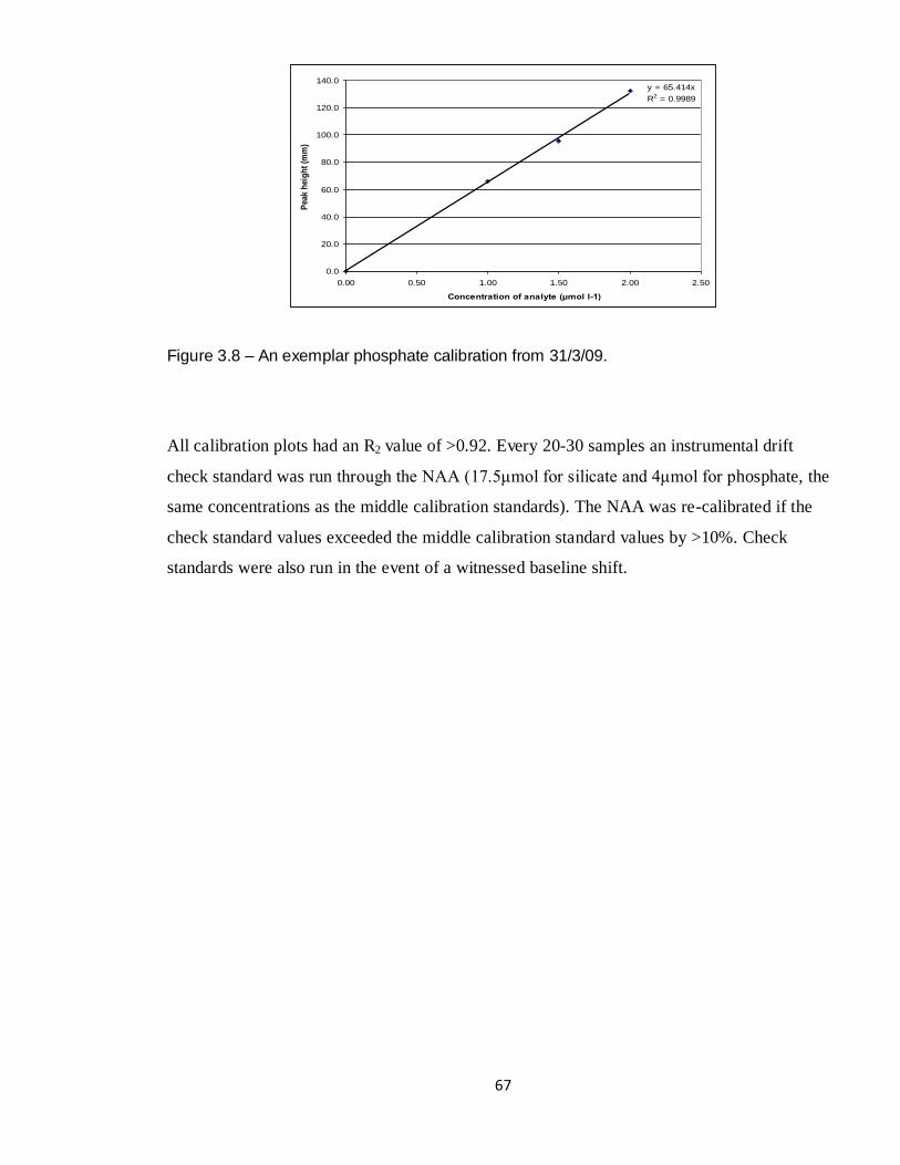
67
Figure 3.8 – An exemplar phosphate calibration from 31/3/09.
All calibration plots had an R2 value of >0.92. Every 20-30 samples an instrumental drift
check standard was run through the NAA (17.5μmol for silicate and 4μmol for phosphate, the
same concentrations as the middle calibration standards). The NAA was re-calibrated if the
check standard values exceeded the middle calibration standard values by >10%. Check
standards were also run in the event of a witnessed baseline shift.
y = 65.414x
R2 = 0.9989
0.0
20.0
40.0
60.0
80.0
100.0
120.0
140.0
0.00 0.50 1.00 1.50 2.00 2.50
Concentration of analyte (μmol l-1)P
eak
hei
gh
t (m
m)

68
3.4.3 Interference Problems
On running oxidised samples through the NAA it was noted that a green colour formed in the
phosphate column (upon reaction of the two phosphate reagents with the sample). In addition
to this mal-formed peaks were formed on the phosphate chart recorder paper:-
Figure 3.9 – Chart recorder paper showing the mal-formed peaks from the phosphate channel when moss oxidations are run through the NAA (time elapsed indicated by black arrow). Four moss oxidations were run through the NAA before the baseline was shifted to the middle of the paper (‘1’). Five more moss oxidations were run through the NAA each showing extremely mal-formed double negative peaks (at ‘2a’ and ‘2b’ the chart recorder pen stuck). The baseline was reset to its normal position at ‘3’.

69
An experiment was designed to determine which chemical interaction was causing the
interference: 1ml of 30% Hydrogen Peroxide solution or 1ml of 30% nitric acid solution was
added to a new centrifuge tube. 1ml of each of the phosphate or silicate reagents was then
added to the centrifuge tubes, the resulting mixture was then shaken by hand. Tubes
containing the phosphate reagents were heated for five minutes in a water bath at 55°C (to
replicate the conditions within the NAA). The colour changes that were observed immediately
upon addition of the phosphate/silicate reagent containing ammonium molybdate tetrahydrate
to hydrogen peroxide can be seen in Figure 3.10 (below):-
A: Phosphate Reagents B: Silicate Reagents
Figure 3.10 – The resulting colour change (extinction) when the phosphate or silicate ammonium molybdate reagent is mixed with 30% hydrogen peroxide (Tubes M-O and S-U, see Table 3.5) versus 30% nitric acid (P-R and V-X) confirms that an interaction between hydrogen peroxide and ammonium molybdate is the source of the extinction. N.B. The tubes in Figure B contain more solution because 1ml of the three silicate reagents was added, as opposed to 1ml of the two phosphate reagents in Figure A. The foam on top of the resulting solutions are a product of the sodium dodecyl sulfate in the NAA reagent mixtures.

70
Sample
Label
Oxidiser Added
(1ml)
Reagents Added
(1ml of each)
M, N, O Hydrogen Peroxide Phosphate
P, Q, R Nitric Acid Phosphate
S, T, U Hydrogen Peroxide Silicate
V, W, X Nitric Acid Silicate
Table 3.5 – Sample labelling regime for the interference determination experiment shown in Figure 3.10.
The experiment shown in Figure 3.10 confirms that a hydrogen peroxide/ammonium
molybdate interaction is the cause of the extinction. Why this extinction appears green inside
the columns of the NAA and yellow inside a centrifuge tube is unknown. A Perkin-Elmer
Lambda 2524
spectrophotometer in visual mode was then used to a run a spectrum scan from
λ 390nm – λ 710nm on samples M through to X. The results are shown in Figures 3.11/12
(below and overleaf).
Figure 3.11 (Left) – The absorbencies across the visual spectrum for the samples containing hydrogen peroxide. Note that all samples show the beginnings of a peak forming at ~515nm reaching maximum amplitude at 391nm.
24 Perkin-Elmer Inc., Shelton, CT 06484, USA.
-0.5
0
0.5
1
1.5
2
2.5
3
390
412
434
456
478
500
522
544
566
588
610
632
654
676
698
Ab
so
rban
ce (
Arb
. U
nit
s)
Wavelength λ (nm)
M
N
O
S
T
U

71
Figure 3.12 (Left) – Absorbencies for samples containing nitric acid. Note that the maximum absorbance is approx. an order of magnitude lower than the maximum absorbance in Figure 3.11.
NB Figures 3.11/12 show absorbencies whereas colour is an emission; therefore the peak will
be expected to form in the area of the spectrum complementary to yellow which is violet (390-
450nm) and it is this region that does indeed contain the highest absorbencies. Figures 3.11/12
are instrumental confirmation that the interference is caused by hydrogen peroxide and not
nitric acid (or at least, to a far lesser extent by nitric acid).
In a second experiment; the phosphate and silicate reagents were added to 1ml of three
oxidised moss samples and three inoculum oxidations. All of these samples turned yellow
(because all of these samples contained hydrogen peroxide within the oxidising mixture), with
the extinction being stronger in some samples than others.
-0.05
0
0.05
0.1
0.15
0.2
0.25
390
412
434
456
478
500
522
544
566
588
610
632
654
676
698
Ab
so
rban
ce (
Arb
. U
nit
s)
Wavelength λ (nm)
P
Q
R
V
W
X

72
3.4.4 NAA Data Calculations
Figure 3.13 (Left) – Stages involved in working up NAA raw data to obtain results in μmol l-1 (grey for silicate, yellow for phosphate) and the blank correction procedure (in blue).
The procedures for working up the silicate NAA
and the phosphate NAA data were different due
to the two different methods of output: the Max
M Raw Value (the photometer absorbance) in
arbitrary units on a VDU for silicate and a height
measured from baseline to peak on chart
recorder paper for phosphate (in mm). Silicate
requires an additional numerical correction for
the baseline, then both sets of data were divided
by the gradient of the relevant calibration plot.
Frequently samples had to be diluted in order to
fit the obtained data within the calibration range
of the NAA (this was particularly the case for
silicate). Where samples were diluted the
resulting data at this point were multiplied by the
dilution factor yielding a concentration in
μmol l-1
.
The blank correcting stages (in blue) are the
same as for the ICP data, however no correction
was required for the upH2O blanks as no silicate
or phosphate could be detected in any upH2O
blank via NAA.

73
3.5 X-Ray Fluorescence Spectroscopy (XRF)
3.5.1 Introduction
Figure 3.14 (below) summarises the key stages in XRF sample preparation:-
Figure 3.14 (Left) – Main stages involved in preparing a fusion bead for XRF analysis
Samples of mineral or rock were dried in an oven at 90°C for five hours
and allowed to cool. The sample was then ground using a Retsch
RS20025
vibratory disc mill set to a programme of 700 r.p.m. for one
minute. 7.6g of Socachim/XRF Scientific26
X-Ray flux was placed into
a platinum/gold crucible. The flux was a certified mixture of 66.0%
lithium tetraborate and 34.0% lithium metaborate. 0.4g of rock sample
was then added to the flux. Great care was taken to record masses
accurately to five decimal places as the precise mass of rock is
important for stoichiometric data analysis. The solution was then mixed
using a metal spatula which had been pre-cleaned with propan-2-ol.
An XRF Scientific Phoenix machine was used to heat the crucibles using butane/oxygen
flames melting the flux and sample and then casting the fusion beads which were subsequently
analysed for the percentage abundance of the „major elements‟ in a sample (that is the 10 most
common elements comprising the Earth‟s crust, see Table 3.6) using a Bruker AXS S4
Pioneer27
XRF spectrometer (NB A more detailed protocol for the entire XRF sample
preparation procedure can be found in Appendix i.ii).
25 Retsch GmbH, Rheinische Strasse 36, 42781 Haan, Germany. 26 XRF Scientific Ltd., Perth, Australia. 27 Bruker AXS Ltd., Banner Lane, Coventry, CV4 9GH, UK.

74
Analyte Species
Magnesium MgO
Aluminium Al2O3
Silicon SiO2
Phosphorus P2O5
Calcium CaO
Titanium TiO2
Manganese MnO
Potassium K2O
Iron Fe2O3
Sodium Na2O
Table 3.6 – The XRF analytes. The resulting percentage by mass data is given in the form of oxidised species due to the fact that the high intensity x-ray beam causes inner electrons to be ejected from the species; forming an oxidised compound (Banwell, 1983).
3.5.2 XRF Data Calculations
Figure 3.15 (overleaf) shows how the original data output of the XRF (in % by mass for an
oxidised compound) was converted into a whole amount in μmol g-1
enabling parity with the
ICP and NAA data (which was worked into whole amounts of analyte in μmol). This was done
by multiplying the XRF output by the total mass of sample (to 5d.p.) then dividing that value
by the total percentage of sample comprising the major analytes (~91%, the other 9%
comprising trace amounts of other elements). The figure obtained was then divided by the
mass of the oxidised XRF analyte yielding a whole amount in mol g-1
which was then
multiplied by 1000 to give an amount in μmol g-1.

75
Figure 3.15 (Left) – Stages in manipulating the XRF data, originally in % by mass to μmol g-1. This enables stoichiometries to be calculated that give parity to the ICP and NAA data (worked up to values in μmol).

76
4: Results and Discussion
4.1 Introduction
Experimental results generally show a strong weathering signal for most analytes on all
substrates. The aggregated data using all experiments conducted on granite, andesite and
vermiculite (except for early experiments in the method development phase or experiments
with a microcosm n<5) are presented in Figures 4.3-4.17. The individual data for the one
chlorite experiment is presented in Figures 4.18/19. Granite and andesite will be the two main
substrates of focus as these substrates have the highest number of experiments conducted upon
them (six and three respectively).
4.2 Statistical Analysis of Experimental Data
4.2.1 Error Bars
4.2.1.1 Aggregated Data
The majority of the graphs presented in this section represent population mean values ( ), i.e.
the mean of all the mean values for all the individual experiments for a given analyte. For
simplicity this data will henceforth be referred to as the „Aggregated Data‟. In graphs of
aggregated data, error bars represent the standard error of the standard deviations of the data
for a given analyte on a given substrate, calculated thus:-
Equation 4.1 – The Standard Error calculation as used to calculate error bars on graphs of aggregated data, where σx,y… are the standard deviations of a specific portion of the dataset in different experiments (e.g. the standard deviation of the Al in W a in the 30/4/08 experiment, the 24/6/08 experiment, the 2/9/08 experiment etc.)

77
All error bars in this section represent the standard error (calculated as shown in Equation 4.1)
unless otherwise stated.
4.2.1.2 Individual Experimental Data
Error bars on graphs for individual experiments represent the 95% confidence interval (or a
probability of the results being due to chance of 5%, P<0.05). The 95% confidence interval
was calculated using Microsoft Excel‟s „tinv‟ function (which gives the Student‟s t value for a
given n at P<0.05) as shown in Equation 4.2 (below):-
Equation 4.2 – Equation for calculating the 95% confidence interval (P<0.05).
4.2.2 Mann-Whitney U Test
SPSS Statistics v17.0 software was used to perform the Mann-Whitney U test on the
experimental data in order to validate or falsify the hypotheses outlined in §1.9, p33 The
Mann-Whitney U test (henceforth referred to as the „U test‟) is a non-parametric technique
that compares the difference between two groups of ranked data as opposed to scaled data
(Pallant, 2007). The U test was chosen over the most appropriate alternative test (the
independent t-test) for two reasons:-
1. Parametric tests (such as t-tests) can only be performed on data that follow a normal
distribution. A large proportion of the data obtained in this procedure is non-Gaussian
in distribution.
2. By substituting non-detects for <LODs an ordinal character has been introduced to the
dataset. The data can no longer be regarded as scaled data in the strictest sense of the
term.

78
The U test (unlike the t-test) compares data by comparing medians as opposed to means (Op.
cit.). The major disadvantage of non-parametric tests over parametric tests is that they are less
sensitive and therefore may not detect differences between two sets of data that actually exist.
The benchmark for statistical significance will be P<0.05 (the probability of results being due
to chance is less than 5%, the 95% confidence interval) with a P<0.01 (a probability of the
results being due to chance of 1%) or lower considered to be a very strong, statistically
significant result. The results of the U test are arranged by experimental substrate later in this
section. The SPSS outputs, including Mann-Whitney U score and the Asymptotic Significance
(P value) are reproduced in Appendix iv.i.
The following U tests were conducted upon the aggregated data for each substrate:-
1. Wa vs. Wb – Abiotic aqueous weathering vs. Total aqueous weathering
2. Wa vs. Wmoss - Abiotic aqueous weathering vs. Weathered analyte uptaken by moss
3. Wb vs. Wmoss – Total aqueous weathering vs. Weathered analyte uptaken by moss
4. Wa vs. Wtot - Abiotic aqueous weathering vs. Total weathering
Tests 1 and 4 are presented in this thesis; test 4 being the most important as it is essentially a
test of the biotic enhancement of weathering factor (Ψ) itself. When considering the P values
obtained from a statistical test it is important to note the direction of the test. For example
whilst conducting the test Wtot vs. Wa for the analyte Al the P value obtained may be 0.05 but
which has the greater median rank Wtot or Wa?
The U test is less reliable if the sample size being tested is less than 30 as SPSS does not
correct for ties (incidences where a value appears more than once) after ranking, it is therefore
inappropriate to apply the U test to data for individual experiments due to the lower sample
size (n). When non-detects are substituted in for <LODs ties occur as the same value is
introduced to the dataset multiple times, this can affect the reliability of the U Test by
rendering statistically significant results insignificant. Incidences where a level of significance
or direction of result appears incongruent with the experimental data and the error bars will be
tested separately using the Independent Samples t-test using SPSS.

79
4.3 Granite Experiments
4.3.1 Introduction
Figure 4.1 – Side and plan views of a granite control microcosm (after a weathering period of 113 days). NB the black flecks in the granite clasts which are the mineral biotite. Condensation on the walls of the jar was removed using swabs and a hairdryer prior to photographing.

80
Figure 4.2 – Plan and side views of mossed granite microcosms shown at time of inoculation (A&B) and after a growth/weathering period of 113 days (C&D). Note the increase in biomass over the weathering period. The moss has yellowed in photos C&D indicating that it has started to die. This was used as an indicator that the microcosms needed sampling.

81
4.3.2 Aggregated Data
In this thesis data are always presented on linear axes and the ICP data always have two
graphs presented one above the other because the values for some analytes were always
substantially higher than the values for others.
The following graphs show the population mean ( ) values for each analyte in all of the
granite experiments except the 15/8/08 experiment that gave anomalous results due to its low
sample size of 2 control microcosms and 2 mossed microcosms. The results are population
means of six experiments (30/3/08, 24/6/08, 2/9/08, 19/12/08, 12/1/09, 30/7/09). Error bars
represent the standard error.
Figure 4.3 (Left) – Population mean ( ) values of the amount of analyte weathered into the different microcosm fractions in the granite microcosms. The aqueous solution from control microcosms (Wa, abiotic weathering) is depicted in light blue bars. The other bar represents total weathering in mossed microcosms (W tot); the purple portion of the bar representing analyte weathered into
aqueous solution (Wb) and the green portion of the bar representing analyte taken up by the moss (Wmoss). Abiotic n=73, Biotic n=66. Mean weathering period = 110 days.

82
Figure 4.3 shows that there are higher amounts of all analytes in biotic granite microcosm
fractions (Wb + Wmoss) compared with the abiotic microcosm fraction (Wa). Al, Fe, K and Mg
are present in higher amounts in the moss than in the biotic microcosm aqueous fraction (the
inverse being true for Ca, Na and Si). On an intra-elemental basis; all error bars are non-
overlapping.
The amounts of analytes contained within moss tissue increased on all substrates compared
with the inoculum at initial conditions. Indeed, the values for analytes contained within the
inoculum used to inoculate that particular set of microcosms are subtracted from the results
obtained for the amounts of analytes within the moss biomass after the weathering period (see
§3.3.3 p60). For example: the mean amount of Fe in the inoculums at initial conditions was
0.05μmol, the mean amount of Fe in moss removed from granite microcosms was 0.28μmol.
A graph of the biotic enhancements of weathering for each analyte can be plotted by
presenting Wa as one bar and Wb and Wmoss as a second stacked bar (henceforth known as
Wtot) and normalising both of these to Wa. By normalising the sum of the biotic microcosm
components to Wa the following operation is performed:-
which is the same as the biotic enhancement of weathering (Ψ) calculation (c.f. Equation 1.8,
p34. The results of this normalisation can be seen in Figure 4.4 (overleaf).

83
Figure 4.4 (Above and Left) – Granite dataset: population means ( ) of the total amounts of analytes weathered into the microcosm fractions normalised to abiotic aqueous weathering (light blue). Total aqueous weathering is represented in purple and analyte uptaken by the moss is represented in green. The amount of analyte weathered into aqueous solutions in control microcosms is normalised to itself and is therefore always 1 (light blue: ‘Abiotic Weathering’). Abiotic n=73, Biotic n=66. Mean weathering period = 110 days.
Figure 4.4 shows that moss biotically enhances the weathering of all analytes on granite; biotic
enhancements (Ψ) are ≈ 1.5 for Ca, Mg, Na and Si, ranging from Ψ1.3 for Na through Ψ16.4
for Al, up to Ψ112.6 for Fe. The magnitude of the biotic enhancement values for Al and Fe are
particularly remarkable considering that granite is widely regarded as being an unlabile
substrate with low weatherability (e.g. Blatt et al. (2006)). Also of particular interest in Figure
4.4 is that two major plant macronutrients (Ca and Mg) are present in lower amounts in the
biotic aqueous fraction than the abiotic aqueous fraction, indicating preferential uptake of Ca
and Mg by the moss (See Figure 4.5, overleaf). Ca and Mg typically form 0.5% and 0.2% of
dry plant tissue respectively (Taiz & Zeiger, 2002). Conversely: Si, Fe and Na are present in

84
higher amounts in the biotic aqueous fraction than the abiotic aqueous fraction indicating that
these analytes are not preferentially uptaken (are „purged‟) by the moss. Si forms 0.1% of dry
plant tissue and is considered a macronutrient, Fe and Na are typically present in dry plant
tissue at levels of 100ppm and 10ppm respectively and are considered plant micronutrients
(Op. cit.).
Figure 4.5 (Left) – Top half of Figure 4.4 reproduced to show which analytes are uptaken by the moss and which are purged by the moss. K is present in approximately equal proportions in the abiotic and the biotic aqueous fractions.
Table 4.1 gives the levels of significance (P values) for the data presented in Figure 4.4 as
obtained by the U test:-
Al Ca Fe K Mg Na Si
Wtot>Wa <0.01 <0.01 <0.01 <0.01 <0.01 <0.01
Wtot<Wa 0.37
Table 4.1 – Levels of significance (P values) for the test W tot vs. Wa in the granite aggregated dataset arranged by direction. (W tot>Wa indicates that the median rank for W tot was higher than the rank for Wa. W tot<Wa indicates the inverse was true). Results rounded to 2 d.p., insignificant results (P>0.05) are italicised.

85
Table 4.1 shows that all analytes except Na show biotic enhancements of weathering that are
significant at the P<0.01 level. This is a highly statistically significant positive result for all
analytes with the exception of Na. The insignificance of the Na result is intriguing given that
the error bars are non-overlapping in Figure 4.1. This result was re-tested using the t test and a
similar insignificant result was obtained (see Appendix iv.ii). A frequency distribution on the
aggregated data for Na revealed that the data follow a log-normal distribution (see Appendix
ii.vii), the population mean ( ) not equaling the population median (2.29μmol and 1.78μmol
respectively).
Figure 4.6 (below) shows the data obtained for silicate and phosphate using the Nutrient Auto-
Analyser (NAA). NB NAA datasets do not contain data for moss because of instrumental
problems caused by a matrix interference (see §3.4.3 p68).
0.00
0.05
0.10
0.15
0.20
0.25
0.30
0.35
0.40
0.45
SiO(4) PO(4)
Mean
am
ou
nt
of
an
aly
te (
µm
ol)
AbioticWeathering
TotalAqueousWeathering
Figure 4.6 – Population mean ( ) of silicate (SiO44-) and phosphate (PO4
3-) weathered into the aqueous solutions in control microcosms (light blue: ‘Abiotic Weathering’) and mossed microcosms (red: Total Aqueous Weathering) in the 30/4/08, 24/6/08 and 2/9/08 granite experiments. NB no PO4
3- was detected in any of the abiotic or biotic samples in the 24/6/08 experiment (See Appendix iii.i.vi). Abiotic n = 34, Biotic n = 31.

86
Figure 4.6 shows aqueous-phase biotic enhancements of weathering for silicate and phosphate
by moss on granite (a 1.6x aqueous phase biotic enhancement for SiO44-
and a 4.2x
enhancement for PO4
3-) though the statistical significance of the phosphate enhancement
appears weak as the standard error bars are very close. The NAA data for silicate is in good
agreement with ICP silicon data (total weathering Si = 0.435μmol, total weathering SiO4 =
0.430μmol). It was expected that the values for NAA silicate would be less than the values
obtained for Si by ICP as the ICP measures total silicon of any speciation, whereas the NAA
only measures silicate (SiO44-
) speciation. Table 4.2 below gives the P values for the test Wa
vs. Wb across all analytes (ICP and NAA):-
Al Ca Fe K Mg Na Si SiO4 PO4
Wb>Wa <0.01 <0.01 0.2 <0.01
Wb<Wa <0.01 0.02 <0.01 <0.01 0.33
Table 4.2 – Levels of significance (P values) for the test Wb vs. Wa in the Granite dataset, arranged by direction. (Wb>Wa indicates that the median rank for Wb was higher than the rank for Wa. Wb<Wa indicates the inverse was true). Results rounded to 2 d.p., insignificant results are italicised.
Table 4.2 shows that the PO43-
weathering enhancement is in fact significant at the P<0.01
level, whereas the enhancement for SiO44-
is statistically insignificant. The standard error bars
are widely distanced in Figure 4.5 so it was suspected that the U test had operated poorly in
this instance. This result was re-tested using the t test and a result in the Wb>Wa direction,
significant at the P<0.05 level was obtained (see Appendix iv.ii). The poor result obtained
using the U test is probably due to the large number of 0 values in the dataset for SiO44-
. The
t test corroborated the P<0.01 result for PO43-
. It should be noted that if the NAA data are
plotted as individual experiments, the 95% confidence error bars for both analytes always
overlap (see Appendix iii.i).

87
4.3.3 Individual Experimental Data
The data from two individual granite experiments (24/6/08 and 12/1/09) are presented in
Figures 4.7/8 below and overleaf:-
Figure 4.7 – (Above and Left) – 24/6/08 granite experiment: arithmetic means ( x ) of the total amounts of
analytes weathered into the abiotic aqueous fraction and the biotic microcosm fractions. Error bars represent the 95% confidence interval. Abiotic n=7, Biotic n=10. Weathering period = 138 days.
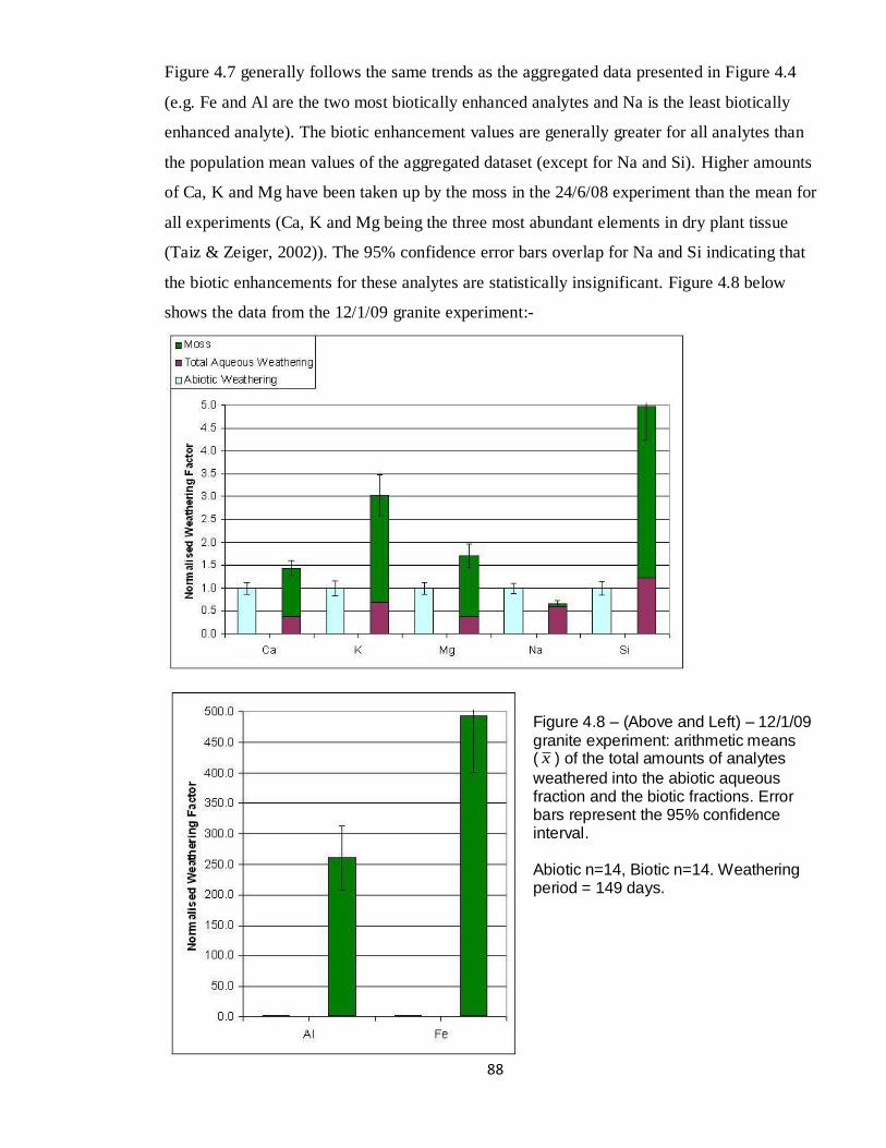
88
Figure 4.7 generally follows the same trends as the aggregated data presented in Figure 4.4
(e.g. Fe and Al are the two most biotically enhanced analytes and Na is the least biotically
enhanced analyte). The biotic enhancement values are generally greater for all analytes than
the population mean values of the aggregated dataset (except for Na and Si). Higher amounts
of Ca, K and Mg have been taken up by the moss in the 24/6/08 experiment than the mean for
all experiments (Ca, K and Mg being the three most abundant elements in dry plant tissue
(Taiz & Zeiger, 2002)). The 95% confidence error bars overlap for Na and Si indicating that
the biotic enhancements for these analytes are statistically insignificant. Figure 4.8 below
shows the data from the 12/1/09 granite experiment:-
Figure 4.8 – (Above and Left) – 12/1/09 granite experiment: arithmetic means ( x ) of the total amounts of analytes
weathered into the abiotic aqueous fraction and the biotic fractions. Error bars represent the 95% confidence interval. Abiotic n=14, Biotic n=14. Weathering period = 149 days.

89
The 12/1/09 experimental data also mirror some of the key trends as the aggregated dataset
(e.g. Al and Fe being the most biotically enhanced analytes). There are two surprising
incongruencies between the 12/1/09 data and the aggregated dataset: the biotic enhancement
(Ψ) for Si in the aggregated data is 1.6 whereas in the 12/1/09 dataset it is 5.0. Furthermore:
there is a Ψ<1 for Na which, given the fact that mosses secrete organic acids that are stronger
than the carbonic acid involved in the abiotic weathering reaction, is a highly unlikely result.
The 12/1/09 experimental data demonstrates the preferential uptake of key plant
macronutrients and the purging of less needed micronutrients better than the 24/6/08
experiment and the aggregated dataset. Figure 4.8 demonstrates uptake of Ca, K and Mg (all
plant macronutrients) and purging of Na and Si.
It should be noted that not all of the individual granite experiments exhibit relationships as
strong as those exhibited by the 24/6/08 and 12/1/09 datasets; the 30/4/08 and 19/12/08 granite
experiments have overlapping 95% confidence limit error bars for five analytes in each
experiment (see Appendix iii.i). Fe however always exhibits a statistically significant biotic
enhancement of weathering in all six granite experiments.
4.3.4 Granite Summary
The biotic enhancement of weathering values for Fe and Al as both a population mean of all
granite experiments (FeΨ=112.6, AlΨ=16.4) and in the individual experiments presented (up
to FeΨ=493.6 in the 12/1/09 experiment, the highest biotic enhancement in any of the granite
experiments) are remarkable given that granite is usually regarded as an unlabile substrate that
is highly resistant to weathering. The additional fact that all results in the Wa vs. Wtot U test for
the aggregated dataset (with the exception of Na) are significant at the P<0.01 level and almost
all error bars are non-overlapping lends weight to the fact that these results are statistically
robust.

90
4.4 Andesite Experiments
4.4.1 Introduction
Figure 4.9 – Side and plan views of an andesite control microcosm shortly after preparation.

91
Figure 4.10 – Plan and side views of mossed andesite microcosms shown at time of inoculation (A&B) and after a growth/weathering phase of 113 days (C&D).
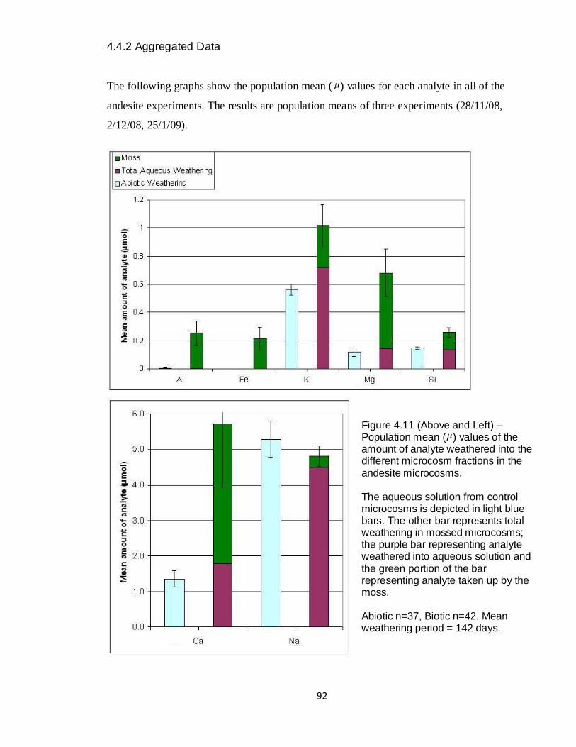
92
4.4.2 Aggregated Data
The following graphs show the population mean ( ) values for each analyte in all of the
andesite experiments. The results are population means of three experiments (28/11/08,
2/12/08, 25/1/09).
Figure 4.11 (Above and Left) – Population mean ( ) values of the amount of analyte weathered into the different microcosm fractions in the andesite microcosms. The aqueous solution from control microcosms is depicted in light blue bars. The other bar represents total weathering in mossed microcosms; the purple bar representing analyte weathered into aqueous solution and the green portion of the bar representing analyte taken up by the moss. Abiotic n=37, Biotic n=42. Mean weathering period = 142 days.

93
Figure 4.12 (below) demonstrates weathering in the three andesite experiments aggregated as
population means and normalised to abiotic weathering:-
Figure 4.12 – Andesite aggregated dataset: population means ( ) of the total amounts of analytes weathered into the different microcosm fractions normalised to abiotic aqueous weathering (light blue). Total aqueous weathering is represented in purple and analyte uptaken by the moss is represented in green. Abiotic n=37, Biotic n=42. Mean weathering period = 142 days.
Figure 4.12 shows that moss biotically enhances the weathering of all analytes on andesite
except for Na (which exhibits a weak negative Ψ of -0.3 with overlapping error bars). Ψ values
range from 4.1 for Ca, through 40.4 for Al up to 330.7 for Fe. The biotic enhancement values
in Figure 4.12 follow a similar pattern to those in the granite aggregated dataset; Al has the
highest Ψ, followed by Fe and then Ca, K and Mg (the comparison of highest-lowest Ψ
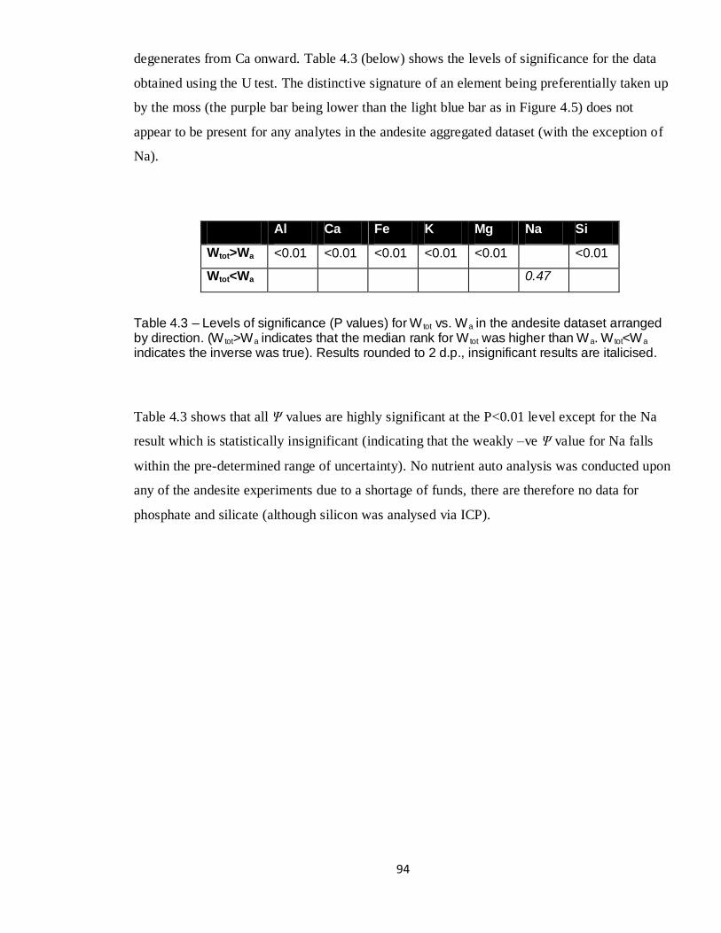
94
degenerates from Ca onward. Table 4.3 (below) shows the levels of significance for the data
obtained using the U test. The distinctive signature of an element being preferentially taken up
by the moss (the purple bar being lower than the light blue bar as in Figure 4.5) does not
appear to be present for any analytes in the andesite aggregated dataset (with the exception of
Na).
Al Ca Fe K Mg Na Si
Wtot>Wa <0.01 <0.01 <0.01 <0.01 <0.01 <0.01
Wtot<Wa 0.47
Table 4.3 – Levels of significance (P values) for W tot vs. Wa in the andesite dataset arranged by direction. (W tot>Wa indicates that the median rank for W tot was higher than Wa. W tot<Wa indicates the inverse was true). Results rounded to 2 d.p., insignificant results are italicised.
Table 4.3 shows that all Ψ values are highly significant at the P<0.01 level except for the Na
result which is statistically insignificant (indicating that the weakly –ve Ψ value for Na falls
within the pre-determined range of uncertainty). No nutrient auto analysis was conducted upon
any of the andesite experiments due to a shortage of funds, there are therefore no data for
phosphate and silicate (although silicon was analysed via ICP).

95
4.4.3 Individual Experimental Data
The data from two individual andesite experiments (2/12/08 and 25/1/09) are presented in
Figures 4.13/14 below and overleaf:-
Figure 4.13 – (Above and Left) – 2/12/08 andesite experiment: arithmetic means ( x )
of the total amounts of analytes weathered into the abiotic aqueous fraction and the biotic microcosm fractions. Error bars represent the 95% confidence interval. Abiotic n=11, Biotic n=9. Weathering period = 202 days.
Figure 4.13 follows the exact same trend as the aggregated data for andesite presented in
Figure 4.12; i.e. the order of biotic enhancement ordered highest-lowest is as follows: Fe, Al,
Mg, Ca, K, Si, Na. All biotic enhancements in the 2/12/08 experiment are higher than those in

96
the aggregated dataset, with more Ca, Mg and Si entering the moss than the average for all
three andesite experiments. The Ψ value for Fe of 625.0 is the highest biotic enhancement
recorded in any experiment conducted on any substrate in this procedure.
Figure 4.14 – (Above and Left) – 25/1/09 andesite experiment: arithmetic means ( x ) of the total amounts of analytes
weathered into the abiotic aqueous fraction and the biotic microcosm fractions. Error bars represent the 95% confidence interval. Abiotic n=24, Biotic n=21. Weathering period = 158 days.
Figure 4.14 also broadly follows the same trends as the aggregated dataset; Fe, Al, Mg and Ca
being the four most biotically enhanced analytes (in that order). The biotic enhancement for K
is extremely marginal in the 25/1/09 experiment (KΨ = 1.03 to 2 d.p. with overlapping error

97
bars). All biotic enhancements are lower than the 2/12/08 experiment, the Ψ value for Fe is
approximately half that of the Ψ value for Fe in the 2/12/08 experiment (339.1 c.f. 625.0). This
decrease in overall Ψ may be a function of weathering period (158 days in the 25/1/09
experiment c.f. 202 days in the 2/12/08 experiment). Figure 4.14 also demonstrates the
preferential uptake of micronutrients (unlike the 2/12/08 data and the aggregated dataset): K,
Ca and Mg appear strongly uptaken (typically forming 1.0%, 0.5% and 0.2% of dry plant
tissue respectively (Taiz & Zeiger, 2002)) with Si being weakly uptaken (0.1% of dry plant
tissue (Op. cit.)).
4.4.4 Andesite Summary
The biotic enhancements of weathering for Fe on andesite were the highest biotic
enhancements encountered across all experiments on all substrates (the highest being FeΨ =
625.0 in the 2/12/08 experiment), the population mean of all three andesite experiments being
FeΨ = 330.7 (this compares with an FeΨ of 112.6 for the granite aggregated dataset). AlΨ on
andesite was approximately double its value on granite. A comparison of the smaller biotic
enhancements in the andesite and granite aggregated datasets is more fluid: SiΨ and NaΨ are
≈ 1.5 in both datasets, the CaΨ and the MgΨ are higher in the andesite dataset than the granite
dataset, but KΨ is slightly lower in the andesite dataset than the granite dataset.
All results in the Wa vs. Wtot U test for the andesite aggregated dataset (with the exception of
Na) are significant at the P<0.01 level and the fact that very few error bars overlap mean that
these data (like those for the granite dataset) are statistically reliable. The 25/1/09
experimental data shows evidence of the preferential uptake of plant macronutrients, such
trends are however not identifiable in the 2/12/08 and the aggregated experimental data.

98
4.5 Vermiculite Experiments
4.5.1 Introduction
Three experiments were conducted using vermiculite. The 18/12/07 experiment provided a
null result due to over-dilution of the sample with upH2O associated with Microcosm water
sampling method 2 (all data points were non-detects). The 14/2/08 experiment yielded positive
results for all analytes and the 17/2/09 experiment yielded positive results for all analytes
except Na. The 14/2/08 and 17/2/09 datasets have been combined to form an aggregated
dataset; however, unlike the aggregated data presented for granite and andesite the error bars
on vermiculite experimental graphs represent the 95% confidence interval as the author felt
that presenting a standard error on a population mean based on two experiments would have
been statistically inappropriate (three experiments being the minimum acceptable for that
method of error representation).
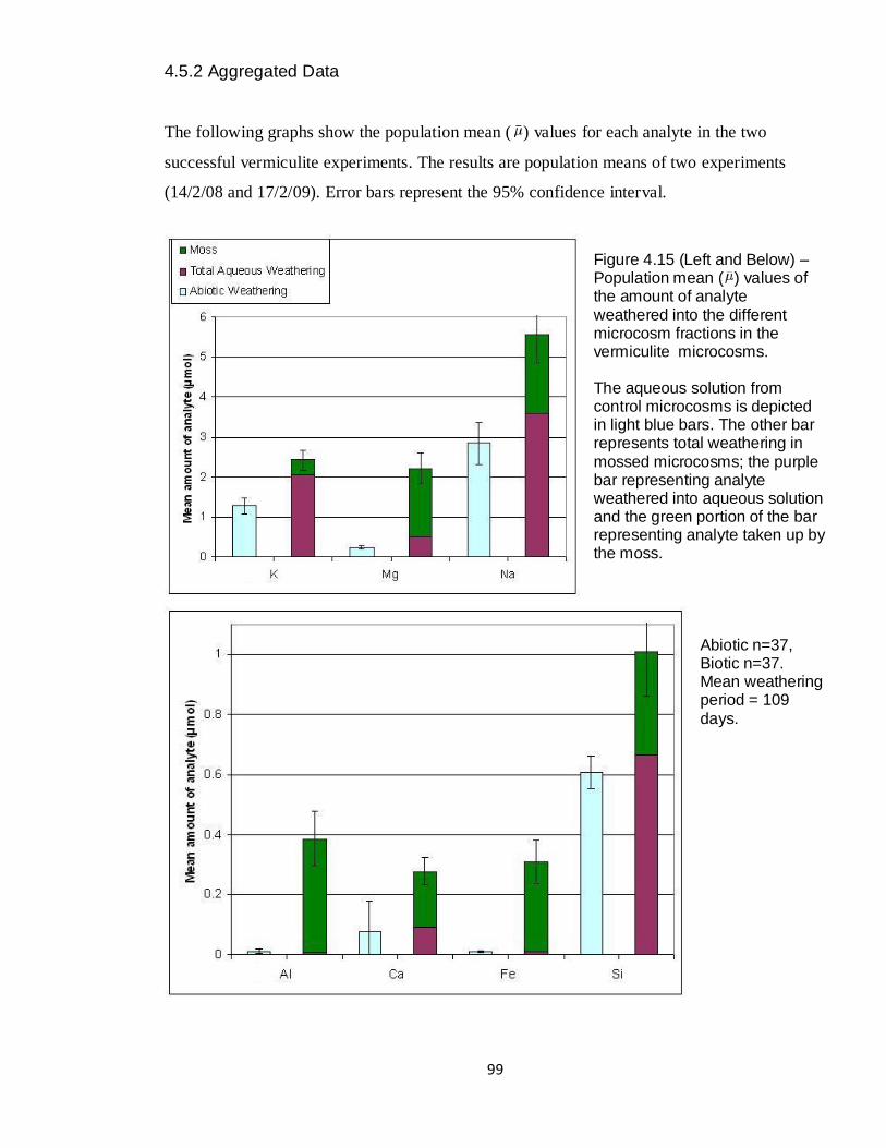
99
4.5.2 Aggregated Data
The following graphs show the population mean ( ) values for each analyte in the two
successful vermiculite experiments. The results are population means of two experiments
(14/2/08 and 17/2/09). Error bars represent the 95% confidence interval.
Figure 4.15 (Left and Below) – Population mean ( ) values of the amount of analyte weathered into the different microcosm fractions in the vermiculite microcosms. The aqueous solution from control microcosms is depicted in light blue bars. The other bar represents total weathering in mossed microcosms; the purple bar representing analyte weathered into aqueous solution and the green portion of the bar representing analyte taken up by the moss.
Abiotic n=37, Biotic n=37. Mean weathering period = 109 days.

100
Figure 4.16 (below) demonstrates weathering in the two vermiculite experiments aggregated
as population means and normalised to abiotic weathering:-
Figure 4.16 (Above and Left) – Vermiculite dataset population means ( ) of the total amount of analyte weathered into the different microcosm fractions normalised to abiotic aqueous weathering (NB error bars represent the 95% confidence interval of the aggregated dataset for each analyte). Abiotic n=37, Biotic n=37. Mean weathering period = 109 days.
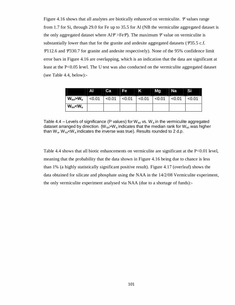
101
Figure 4.16 shows that all analytes are biotically enhanced on vermiculite. Ψ values range
from 1.7 for Si, through 29.0 for Fe up to 35.5 for Al (NB the vermiculite aggregated dataset is
the only aggregated dataset where AlΨ >FeΨ). The maximum Ψ value on vermiculite is
substantially lower than that for the granite and andesite aggregated datasets (Ψ35.5 c.f.
Ψ112.6 and Ψ330.7 for granite and andesite respectively). None of the 95% confidence limit
error bars in Figure 4.16 are overlapping, which is an indication that the data are significant at
least at the P<0.05 level. The U test was also conducted on the vermiculite aggregated dataset
(see Table 4.4, below):-
Al Ca Fe K Mg Na Si
Wtot>Wa <0.01 <0.01 <0.01 <0.01 <0.01 <0.01 <0.01
Wtot<Wa
Table 4.4 – Levels of significance (P values) for W tot vs. Wa in the vermiculite aggregated dataset arranged by direction. (W tot>Wa indicates that the median rank for W tot was higher than Wa. W tot<Wa indicates the inverse was true). Results rounded to 2 d.p.
Table 4.4 shows that all biotic enhancements on vermiculite are significant at the P<0.01 level,
meaning that the probability that the data shown in Figure 4.16 being due to chance is less
than 1% (a highly statistically significant positive result). Figure 4.17 (overleaf) shows the
data obtained for silicate and phosphate using the NAA in the 14/2/08 Vermiculite experiment,
the only vermiculite experiment analysed via NAA (due to a shortage of funds):-

102
Figure 4.17 (Left) – Arithmetic mean values ( x ) of
silicate (SiO44-)
and phosphate (PO4
3-) weathered into aqueous solution in control microcosms in the 14/2/08 Vermiculite experiment (NB error bars represent the 95% confidence interval).
Abiotic n = 20, Biotic n=20.
Al Ca Fe K Mg Na Si SiO4 PO4
Wb>Wa <0.01 <0.01 <0.01 0.146
Wb<Wa <0.01 0.383 <0.01 <0.01 <0.01
Table 4.5 – P values for Wb vs. Wa in the 14/2/08 Vermiculite dataset arranged by direction.
Table 4.5 shows that the result for PO4 is not significantly different and SiO44-
is present at a
higher level in Wa than Wb (P<0.01). Given the fact that no PO4 was detected in any of the
abiotic aqueous fractions and a mean of 0.53μmol was detected into the biotic aqueous
fraction; this appears to be another spurious U test result (probably due to the large number of
0 values in the Wa dataset and because SPSS does not correct for ties where n<30). This result
was re-tested using the t test and a P<0.01 result in the Wb>Wa direction was obtained (see
Appendix iv.ii). The t test also showed that SiO44-
Wb>Wa, but this result is statistically
insignificant at the P<0.05 level.
0.00
0.10
0.20
0.30
0.40
0.50
SiO(4) PO(4)
Me
an
am
ou
nt
of
an
aly
te (
µm
ol)
Abiotic
Weathering
Total
Aqueous
weathering

103
4.5.3 Vermiculite Summary
Even though a third experiment for vermiculite is lacking; it appears that the vermiculite
aggregated dataset is robust: no error bars overlap on the ICP data (Figure 4.15/6) and all
biotic enhancements yield P values of <0.01 after testing with the U test (Table 4.5). The weak
aqueous phase biotic enhancement for silicate is statistically insignificant (overlapping error
bars and T test gives a P>0.05). The 5.3x aqueous phase biotic enhancement of phosphate is
highly statistically significant (t test P<0.01). The vermiculite data do not show evidence for
the preferential uptake of plant macronutrients by moss.

104
4.6 Chlorite Experiment
Figure 4.18 (below) represents data from the one experiment started on 24/6/08 using a rock
that contained the mineral chlorite:-
Figure 4.18 (Above and Left) - 24/6/08 Chlorite experiment: arithmetic means ( x ) of the amount
of analyte weathered into the different microcosm fractions in the chlorite microcosms. (NB error bars represent the 95% confidence interval). The aqueous solution from control microcosms is depicted in light blue bars. The other bar represents total weathering in mossed microcosms; the purple bar representing analyte weathered into aqueous solution and the green portion of the bar representing analyte taken up by the moss. Abiotic n=7, Biotic n=7.
Weathering period = 72 days.

105
Figure 4.19 (Above and Left) – 24/6/08 Chlorite experiment: arithmetic means ( x ) for the total
amount of analyte weathered into the different microcosm fractions normalised to abiotic aqueous weathering (NB error bars represent the 95% confidence interval). Abiotic n=7, Biotic n=7. Weathering period = 72 days.
Figure 4.19 demonstrates Ψ values ranging from 1.1 for Si up to 38.3 for Fe. All 95%
confidence interval error bars are non-overlapping, with the exception of Na and Si (which
had the smallest biotic enhancements). The chlorite containing rock was cut into rectangular
prisms and was very glassy (vitreous) in nature indicating that it was highly felsic (contained a
high proportion of SiO2). Rocks containing a high proportion of SiO2 are very difficult to
weather, which may explain the lower maximum biotic enhancement encountered on chlorite
relative to the other substrates.
Figure 4.19 shows the preferential weathering signal for all analytes except Fe and Si
(including Na which is a micronutrient usually present in dry plant tissue at lower amounts

106
than Fe). Al shows signs of preferential uptake by the moss even though it is not generally
considered a plant nutrient (Taiz & Zeiger, 2002). This almost universal demonstration of
preferential weathering could be a response by the moss to the highly unlabile nature of the
felsic chlorite rock; the moss could be exerting a strong weathering effect upon the substrate
and in the process taking up nutrients in larger amounts than it requires.
The U test was conducted upon the chlorite dataset but it is important to note that the sample
size of only seven mossed and seven control microcosms is very low and so statistical analysis
of the dataset should be treated with caution.
Al Ca Fe K Mg Na Si
Wtot>Wa <0.01 <0.01 <0.01 <0.01 <0.01 0.32
Wtot<Wa 0.90
Table 4.6 – Levels of significance (P values) for W tot vs. Wa in the 24/6/08 Chlorite dataset arranged by direction. (W tot>Wa indicates that the median rank for W tot was higher than Wa. W tot<Wa indicates the inverse was true). Results rounded to 2 d.p., insignificant results are italicised.
Table 4.6 demonstrates that all positive results were significant at the P<0.01 level except for
Na and Si which are insignificant. Whilst the low sample size means that the analysis
presented in Table 4.6 should be treated with caution, the data in Table 4.6 are congruent with
the 95% confidence limit error bars on Figure 4.19. The NAA PO4 and SiO4 data were both
statistically insignificant, most likely due to the low sample size. These data are not presented
here but are presented in Appendix iii.iv.
Considering the highly felsic nature of the chlorite rock, the results presented here are
impressive. A repeat experiment with a greater sample size would be highly informative.

107
4.7 Inoculum only experiment
4.7.1 Introduction
On 30/7/09 a batch of moss inoculum and filtrate was used to prepare 15 granite mossed and
15 granite control microcosms. On this day the same volume of inoculum as was added to
mossed microcosms (3ml) was added to microcosm containers which did not contain any
substrate. The procedures were standardised in all respects, the only exception being that a
substrate was not added to the no substrate or „bare‟ microcosms prior to inoculation. After 50
days the moss in the bare microcosms had died, so all microcosms initiated on 30/7/09 were
sampled at this point (NB this was a much shorter weathering period than the mean 112 days
when a substrate was present. The data from the 30/7/09 experiments are presented in Figure
4.20 (overleaf).

108
4.7.2 Experimental Data
Figure 4.20 – Amount of analyte in the mossed microcosm components from bare microcosms (grey and blue) and the mossed microcosm components from granite microcosms (dark green and burgundy) in the 30/7/09 experiments. The sum of analyte within both mossed microcosm components is regarded as ‘Total Weathering’ or W tot. Error bars represent the W tot 95% confidence limit. Bare n=14, Granite n=14. Weathering period = 50 days.
The most noticeable facet of the data presented in Figure 4.20 (above) is that all analytes are
present in much higher amounts in the biotic components from granite microcosms than the
biotic components from bare microcosms. The amounts of analytes (μmol) weathered in
granite microcosms is statistically greater than the amounts weathered in bare microcosms at
the 95% confidence interval for all analytes except for Na (error bars overlap). The
concentration of analyte in the fractions from all microcosms has been corrected for blanks
(See Figure 3.3 p60) and therefore the amounts of analytes in bare microcosm fractions must
result from contamination from the microcosm jars themselves or additional contamination
that occurred during sampling (every effort was made to minimise this using a semi-clean
technique). Figure 4.20 shows that this contamination was, for the most part, very small, the

109
exception being Na (1.83μmol). Figure 4.21 (below) represents the granite and bare
microcosm Wtot data, normalised to bare Wtot.
Figure 4.21 – Mean total weathering in the 30/7/09 bare microcosms normalised to itself (grey bar) versus mean total weathering in the 30/7/09 granite microcosms normalised to bare W tot (russet coloured bar). NB Error bars are 95% confidence limits normalised to bare W tot. Bare n=14, Granite n=14. Weathering period = 50 days.
Figure 4.21 demonstrates the differences in ionic dissolution when a substrate is present
(russet) compared with when a substrate is absent (grey). Bare:Granite weathering
enhancement factors range from 1.5 for Na (overlapping 95% confidence limit bars) to 111.7
for Si. The Si enhancement is perhaps unremarkable as Si is the primary constituent of granite
(and indeed any rock/mineral) after oxygen (Blatt et al., 2006). The increase in amounts of

110
analytes entering solution and being taken up by moss when granite is present compared to
when no substrate is present is striking. A U test was performed comparing the 30/7/09
Granite Wtot with the 30/7/09 Bare Wtot, the results obtained are presented in Table 4.7
(below).
Al Ca Fe K Mg Na Si
Granite>Bare <0.01 <0.01 <0.01 <0.01 <0.01 0.03 <0.01
Granite<Bare
Table 4.7 – Levels of significance (P values) for W tot in the granite dataset vs. W tot in the bare dataset arranged by direction. Granite>Bare indicates that the median rank for Granite W tot was higher than that for Bare W tot. Granite<Bare indicates the inverse was true. Results rounded to 2 d.p.
4.7.3 Summary
Table 4.7 demonstrates that Wtot in granite microcosms was greater than Wtot on bare
microcosms and that this result is statistically significant for all analytes except Na at the
P<0.01 level. The Na result is statistically significant at the P<0.05 level. Figure 4.20/1 and
Table 4.7 taken collectively demonstrate that the effects observed in the microcosm
experiments occur as a result of the weathering of the substrate and are not (for example) an
effect of ions diffusing out of the moss during growth.

111
4.8 Masses of moss recovered
Table 4.8 (below) shows the mean mass of moss obtained from the microcosm experiments
arranged by substrate with the mean mass of moss inoculum at initial conditions for
comparison:-
Mean amount of
moss recovered
(mg)
Sample size
(n)
σ
Inoculum 4.12 4 1.10
Granite 17.92 70 19.21
Basalt 15.07 6 4.02
Andesite 11.17 42 10.61
Chlorite 10.94 8 2.49
Vermiculite 3.24 49 2.96
Table 4.8 – Mean amounts of moss recovered from mossed microcosms (mg) by analyte. ‘Inoculum’ gives mass of 3ml of moss inoculum at the time of inoculation. NB the mean amount of moss recovered from mossed vermiculite microcosms falls below the inoculum mean due to the vastly reduced recovery efficiency associated with this fine-grained, highly exfoliated substrate (see §2.8 p47).
The difference between the „Inoculum‟ and the mean amounts of moss recovered can be taken
as a crude indicator of carbon fixation and growth. Caution must however be observed here as
the inoculum comparison n is small (this represented two pseudo-replicated aliquots of
inoculums prepared on 7/5/08 and 23/6/08 respectively). However, the means of moss
recovered are under-estimates of the actual biomass grown as not all of the moss was
recovered during microcosm sampling. In experiments such as this, a substantial portion of the
rooting structure is always irrecoverable (c.f. other studies such as Lewis & Quirk (1967)).

112
4.9 Weathering per unit Moss Biomass
4.9.1 Introduction
After the weathering period the moss biomass was removed from the microcosm, the moss
was weighed and the mass of moss was recorded prior to the moss being oxidised in a mixture
of acids. If the chemical data are normalised to the mass of moss biomass recovered then the
data presented in Tables 4.9-4.12 is obtained. Such analyses are important in modelling terms
as they enable calculation of the likely amount of an analyte weathered per unit mass of moss
biomass grown on Earth‟s surface.
4.9.2 Normalised data
Al Ca Fe K Mg Na Si
Wa 0.012
(±0.026)
1.664
(±0.172)
0.002
(±0.002)
0.669
(±0.031)
0.427
(±0.047)
2.908
(±0.441)
0.346
(±0.072)
Wb 0.013
(±0.005)
1.252
(±0.374)
0.005
(±0.003)
0.658
(±0.096)
0.344
(±0.124)
3.120
(±0.349)
0.435
(±0.111)
Wmoss
(per mg)
0.017
(±0.002)
0.109
(±0.008)
0.022
(±0.002)
0.101
(±0.008)
0.031
(±0.002)
0.044
(±0.025)
0.012
(±0.001)
Table 4.9 – Granite aggregated data (to 3d.p.) values in μmol except for Wmoss (values in μmol/mg). ± value is the standard error (instances where SE≥value are italicised).
The data in Table 4.9 will be used to place weathering within a whole Earth context in §5.2 of
the Conclusions.

113
Al Ca Fe K Mg Na Si
Wa 0.006 (±0.001)
1.356 (±0.221)
0.001 (±1.76 E-21)
0.563 (±0.037)
0.119 (±0.029)
5.292 (±0.518)
0.148 (±0.007)
Wb 0.006 (±2.86 E-4)
1.798 (±0.154)
0.001 (±9.31 E-2)
0.720 (±0.029)
0.144 (±0.013)
4.490 (±0.376)
0.137 (±0.001)
Wmoss
(per mg) 0.042 (±0.010)
0.535 (±0.116)
0.035 (±0.010)
0.073 (±0.015)
0.089 (±0.018)
0.042 (±0.002)
0.022 (±0.004)
Table 4.10 – Andesite aggregated data (to 3d.p.) values in μmol except for Wmoss (values in μmol/mg). ± value represents the standard error (instances where SE≥value are italicised). Where SE is 0 to 3d.p. the figure is given in scientific notation.
Al Ca Fe K Mg Na Si
Wa 0.011 (±0.012)
0.079 (±0.204)
0.011 (±1.35 E-4)
1.323 (±0.086)
0.240 (±0.019)
2.942 (±0.480)
0.606 (±0.072)
Wb 0.005 (±0.003)
0.089 (±0.003)
0.009 (±0.003)
2.046 (±0.267)
0.499 (±0.081)
3.607 (±0.592)
0.654 (±0.073)
Wmoss
(per mg) 0.161 (±0.065)
0.083 (±0.016)
0.125 (±0.026)
0.172 (±0.085)
0.710 (±0.165)
1.060 (±1.346)
0.172 (±0.145)
Table 4.11 – Vermiculite aggregated data (to 3d.p.) values in μmol except for Wmoss (values in μmol/mg). ± value is the standard error (instances where SE≥value are italicised). Where SE
is 0 to 3d.p. the figure is given in scientific notation.
The larger number of instances of the standard error exceeding the values in Table 4.11
compared with Tables 4.9 and 4.10 for vermiculite is likely due to the reduced recovery
efficiency for moss from vermiculite mossed microcosms and the fact that the summary data
only represents two experiments whereas the andesite dataset represents three experiments and
the granite dataset six experiments.
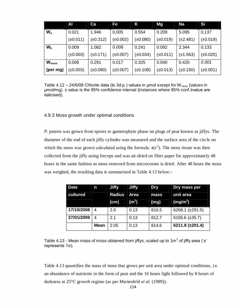
114
Al Ca Fe K Mg Na Si
Wa 0.021
(±0.011)
1.946
(±0.312)
0.005
(±0.002)
0.554
(±0.080)
0.209
(±0.019)
5.095
(±2.481)
0.137
(±0.019)
Wb 0.009
(±0.003)
1.082
(±0.171)
0.006
(±0.007)
0.241
(±0.034)
0.092
(±0.011)
2.344
(±1.563)
0.133
(±0.020)
Wmoss
(per mg)
0.008
(±0.003)
0.291
(±0.090)
0.017
(±0.007)
0.325
(±0.108)
0.040
(±0.013)
0.420
(±0.150)
0.001
(±0.001)
Table 4.12 – 24/6/08 Chlorite data (to 3d.p.) values in μmol except for Wmoss (values in μmol/mg). ± value is the 95% confidence interval (instances where 95% conf.≥value are italicised).
4.9.3 Moss growth under optimal conditions
P. patens was grown from spores to gametophyte phase on plugs of peat known as jiffys. The
diameter of the end of each jiffy cylinder was measured and the surface area of the circle on
which the moss was grown calculated using the formula: π(r2). The moss tissue was then
collected from the jiffy using forceps and was air-dried on filter paper for approximately 48
hours in the same fashion as moss removed from microcosms is dried. After 48 hours the moss
was weighed, the resulting data is summarised in Table 4.13 below:-
Date
cultured
n Jiffy
Radius
(cm)
Jiffy
Area
(m2)
Dry
mass
(mg)
Dry mass per
unit area
(mg/m2)
17/10/2008 4 2.0 0.13 816.5 6268.1 (±291.5)
27/01/2009 4 2.1 0.13 812.7 6155.6 (±35.7)
Mean 2.05 0.13 814.6 6211.8 (±201.4)
Table 4.13 - Mean mass of moss obtained from jiffys, scaled up to 1m2 of jiffy area (‘±’ represents 1σ).
Table 4.13 quantifies the mass of moss that grows per unit area under optimal conditions, i.e.
an abundance of nutrients in the form of peat and the 16 hours light followed by 8 hours of
darkness at 25°C growth regime (as per Marienfeld et al. (1989)).

115
4.9.4 Utilising normalised data
To test the appropriateness of presenting the biotic weathering data normalised to mass of
moss recovered the amounts of each analyte were plotted against the mass of moss recovered
from that microcosm (see Figures 4.22/23 below).
Figure 4.22 (Left) – Amounts of Fe in moss (μmol) from all granite microcosms plotted against the mass of moss (mg) recovered from the microcosm.
Figure 4.23 (Left) – Amounts of Si in the biotic aqueous fraction (μmol) from all granite microcosms plotted against the mass of moss (mg) recovered from the microcosm.
Figures 4.22/23 demonstrate the strongest positive correlation co-efficients obtainable for
analytes in moss and the biotic aqueous fraction respectively. The figures demonstrate a
positive relationship between mass of moss (mg) and the amount of analyte (μmol) (which is
to be expected because the greater the mass of moss oxidised, the greater the amount of
y = 0.0136x + 0.0983
R2 = 0.1847
0
0.1
0.2
0.3
0.4
0.5
0.6
0.7
0.8
0.00 5.00 10.00 15.00 20.00 25.00 30.00
Mass of moss (mg)
Am
ou
nt
of
Fe (
µm
ol)
y = 0.0219x + 0.2095
R2 = 0.0438
0
0.5
1
1.5
2
2.5
3
0.00 5.00 10.00 15.00 20.00 25.00 30.00
Mass of moss (mg)
Am
ou
nt
of
Si
(µm
ol)
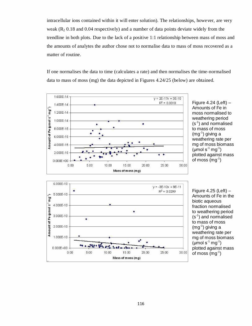
116
intracellular ions contained within it will enter solution). The relationships, however, are very
weak (R2 0.18 and 0.04 respectively) and a number of data points deviate widely from the
trendline in both plots. Due to the lack of a positive 1:1 relationship between mass of moss and
the amounts of analytes the author chose not to normalise data to mass of moss recovered as a
matter of routine.
If one normalises the data to time (calculates a rate) and then normalises the time-normalised
data to mass of moss (mg) the data depicted in Figures 4.24/25 (below) are obtained.
Figure 4.24 (Left) – Amounts of Fe in moss normalised to weathering period (s-1) and normalised to mass of moss (mg-1) giving a weathering rate per mg of moss biomass (μmol s-1 mg-1) plotted against mass of moss (mg-1)
Figure 4.25 (Left) – Amounts of Fe in the biotic aqueous fraction normalised to weathering period (s-1) and normalised to mass of moss (mg-1) giving a weathering rate per mg of moss biomass (μmol s-1 mg-1) plotted against mass of moss (mg-1)
117
Figures 4.24/25 indicate that time normalising the data prior to mass normalisation establishes
even weaker relationships than those established by mass normalisation alone (R2 0.002 and
-0.03 respectively). Figure 4.25 demonstrates a negative relationship between mass of moss
and amount of Fe per unit time and mass that is clearly erroneous.
4.10 Stoichiometries
4.10.1 Substrate Petrologies
At least two samples of washed and unwashed granite, andesite and vermiculite were analysed
using X-Ray Fluorescence Spectroscopy (XRF). Two samples of unwashed chlorite were also
analysed using XRF. There was no significant difference between washed and unwashed
samples (all samples fell within ±1σ of the mean of the washed and unwashed samples added
together, see Appendix iv.iii), the data was therefore aggregated together and a mean taken in
order to provide a larger n upon which error analysis could be reliably performed.
Table 4.14 (overleaf) shows the mean amounts of the ten major crustal elements (those found
in greatest abundance in the Earth‟s crust) for three experimental substrates with
corresponding reference values for those substrates:-

118
Granite Granite
Ref.28
Andesite Andesite
Ref.29
Vermic. Vermic.
Ref.30
MgO 0.43 0.71 3.02 0.12 20.92 16-35
Al2O3 15.67 14.42 15.18 15.57 8.66 10-16
SiO2 69.76 72.04 59.05 60.34 34.86 38-46
P2O5 0.24 0.12 0.26 0.28 0.08 ?
CaO 0.81 1.82 4.50 5.20 0.38 1-5
TiO2 0.24 0.30 0.71 0.72 1.00 1-3
MnO 0.04 0.05 0.12 0.19 0.05 ?
K2O 5.32 4.12 2.11 1.88 5.07 1-6
Fe2O3 1.73 1.22 5.86 6.07 7.69 6-13
Na2O 3.19 3.69 4.07 3.62 0.63 ?
Other 2.58 1.51 5.14 6.01 20.65 ?
Table 4.14 – The amount of analytes (wt. %) in three experimental substrates as measured by XRF compared with reference values for those substrates.
Table 4.14 shows that the XRF analyses are, for the most part, congruent with reference
values, with some outliers (often amongst the trace elements comprising the rock/mineral).
Table 4.15 (overleaf) gives the XRF data for the experimental substrates in μmol g-1
to
facilitate comparison with experimental values.
28 Source: Blatt et al. (2006). 29 Source: Wainwright (2010). 30 Source: TVA (2010)
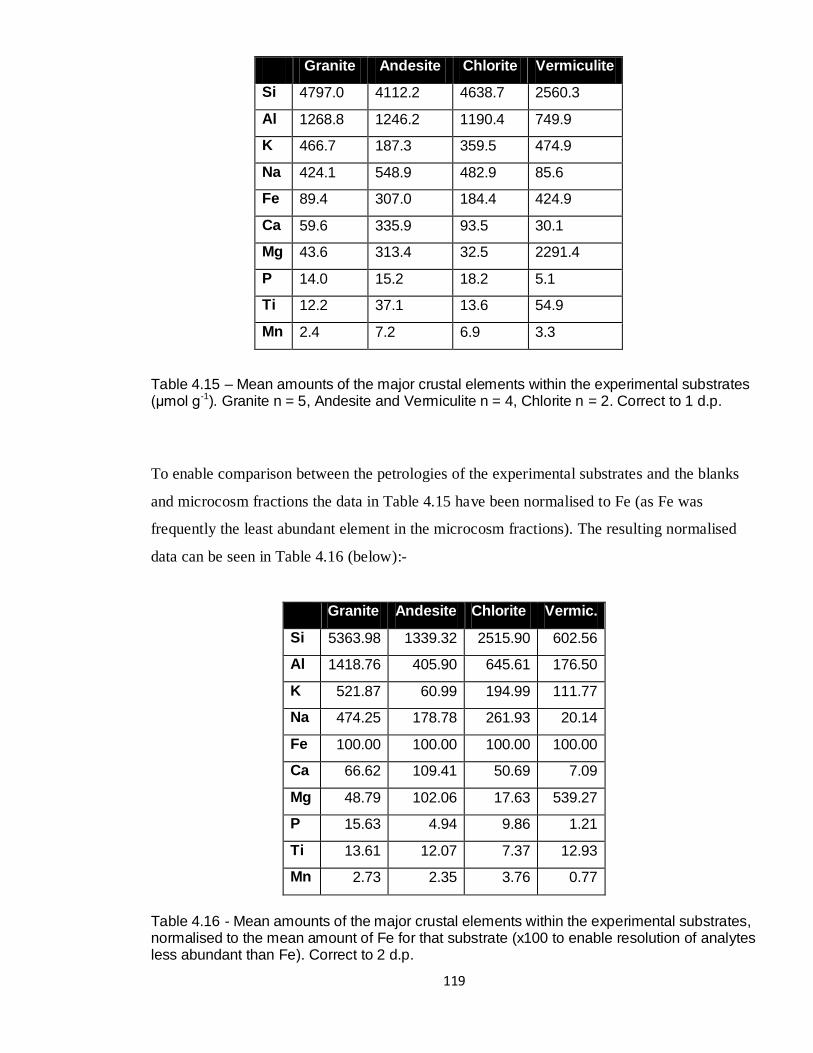
119
Granite Andesite Chlorite Vermiculite
Si 4797.0 4112.2 4638.7 2560.3
Al 1268.8 1246.2 1190.4 749.9
K 466.7 187.3 359.5 474.9
Na 424.1 548.9 482.9 85.6
Fe 89.4 307.0 184.4 424.9
Ca 59.6 335.9 93.5 30.1
Mg 43.6 313.4 32.5 2291.4
P 14.0 15.2 18.2 5.1
Ti 12.2 37.1 13.6 54.9
Mn 2.4 7.2 6.9 3.3
Table 4.15 – Mean amounts of the major crustal elements within the experimental substrates (μmol g-1). Granite n = 5, Andesite and Vermiculite n = 4, Chlorite n = 2. Correct to 1 d.p.
To enable comparison between the petrologies of the experimental substrates and the blanks
and microcosm fractions the data in Table 4.15 have been normalised to Fe (as Fe was
frequently the least abundant element in the microcosm fractions). The resulting normalised
data can be seen in Table 4.16 (below):-
Granite Andesite Chlorite Vermic.
Si 5363.98 1339.32 2515.90 602.56
Al 1418.76 405.90 645.61 176.50
K 521.87 60.99 194.99 111.77
Na 474.25 178.78 261.93 20.14
Fe 100.00 100.00 100.00 100.00
Ca 66.62 109.41 50.69 7.09
Mg 48.79 102.06 17.63 539.27
P 15.63 4.94 9.86 1.21
Ti 13.61 12.07 7.37 12.93
Mn 2.73 2.35 3.76 0.77
Table 4.16 - Mean amounts of the major crustal elements within the experimental substrates, normalised to the mean amount of Fe for that substrate (x100 to enable resolution of analytes less abundant than Fe). Correct to 2 d.p.

120
The data in Table 4.16 can be used to form stoichiometric formulae for each of the substrates
(in a similar approach to Sterner & Elser (2002)) thus:-
Granite – (Si54 Al14 K5 Na5 Fe1)100 (Ca7 Mg5 P2 Ti1)10 Mn3
Andesite – (Si13 Al4 Na2 Ca1 Mg1 Fe1)100 (K6 Ti1)10 P5 Mn2
Vermiculite – (Si6 Mg5 Al2 K1.1 Fe1.0)100 (Na2 Ti1)10 Ca7 P1 Mn1
Chlorite – (Si25 Al6 Na3 K2 Fe1)100 (Ca5 Mg2 P1)10 Ti7 Mn1
Equations 4.3 – Stoichiometric formulae for four of the experimental substrates calculated using data from XRF analyses, relative to Fe. Numbers given to 1 significant figure and are arranged in order of stoichiometric abundance.
The formulae in Equations 4.3 can be read thus: for every atom of iron (Fe) in granite there are
54 atoms of silicon (Si). For every 100 atoms of iron there are three of manganese (Mn) etc.
Some facets of the stoichiometries presented in Equations 4.3 can be easily explained
petrologically e.g. Si is always the most abundant XRF analyte in each substrate and
aluminium (Al) is the second most abundant element in all substrates with the exception of
vermiculite. This can be explained by the fact that Al readily isomorphically substitutes in-
between SiO4 tetrahedra in plate silicates (Andrews et al., 2004). Also the fact that Mg is the
second most abundant analyte in vermiculite is explained by the fact that it is the main inter-
sheet cation in vermiculite (Deer et al., 1966), hence why Mg is the second most abundant
element in vermiculite rather than Al.
Broadly; the stoichiometries of granite, andesite and chlorite are similar with respect to the
most abundant and least abundant elements, with no concordance for the other elements. The
pattern followed can be described thus:-
Si, Al,… Ti… Mn.

121
4.10.2 Stoichiometries of the Microcosmal Fractions and Blanks
The stoichiometries of blanks of moss inoculum and filtrate (i.e that which was added to
mossed and control microcosms respectively) and the stoichiometries of the microcosm
fractions (i.e. the aqueous solutions resulting from control and mossed microcosms and the
moss from mossed microcosms) were analysed in order to provide an indication of any trends
that exist in the order of elemental abundance and the relative abundance of the elements
themselves at an intra-elemental level, which could be indicative of weathering. NB All
analysis of blanks and microcosm components was by ICP, with the exception of analysis for
P which was by NAA (where such data are available). The typical stoichiometry of dry plant
tissue can be given as:-
(K13 Ca7 Mg4 P3 Si2 Fe1)100 Na20 Al2
Equation 4.4 – Stoichiometric ratio of the experimental analytes as commonly found in dry plant tissue, relative to Fe (data from Taiz & Zeiger (2002)). Note that the most abundant elements K to Si are the plant macronutrients.
The mean of inoculum initial conditions samples analysed in round 5 differs substantially
from those analysed in rounds 8&9. The mean stoichiometries of inoculums analysed in
rounds 5 and rounds 8&9 respectively, relative to Fe, are given in Equations 4.5 (below).
Round 5 – (Na17 Ca6 Mg3 K2 Fe1)100 Al16 Si4
Rounds 8&9 – (Ca13 K12 Mg5 Fe1)100 Na55 Al12 Si2
Equations 4.5 – Stoichiometric formulae for the moss inoculums at initial conditions, arranged by the ICP round the inoculums were analysed in, relative to Fe. Numbers given to 1 significant figure and are arranged in order of stoichiometric abundance.

122
In both sets of inoculums Al and Si are the least abundant analytes. Na was far more abundant
in the round 5 inoculums, but was much less abundant in the rounds 8&9 inoculums. The
reasons for this are unclear except that instrumental problems can be ruled out as other
samples were unaffected. There is some congruity between the rounds 8&9 inoculums and
Equation 4.4 in that the plant macronutrients are more abundant in the rounds 8&9 inoculums
(a noticeable incongruity being that Si is the least abundant analyte in the inoculums yet is a
plant macronutrient).
The stoichiometry of the filtrate initial conditions samples (calculated using a median of all
samples taken in the procedure, is as follows):-
(K10 Na10 Ca6 Mg2 Si2)100 Fe10 Al7
Equation 4.6 – Stoichiometric formula for filtrate at initial conditions, relative to Fe. Numbers given to 1 significant figure and are arranged in order of stoichiometric abundance.
The filtrate and the inoculum differ in the fact that the filtrate is what remains after the
inoculum has been passed through a 0.2μm filter (the filtrate is devoid of biota). When
Equation 4.6 is compared with Equations 4.5 it is clear that the presence of biota in the form of
moss does affect the stoichiometry of the suspension (e.g. Si is about an order of magnitude
more abundant in the filtrate than in the inoculums; there are 20 atoms of Si for every 1 of Fe
in the filtrate, yet there are 2-4 atoms of Si for every 100 of Fe in the moss inoculums).
4.10.3 Microcosmal Stoichiometry Summary
If substrate petrology is compared with the stoichiometries of the microcosmal fractions
connected with that substrate it is possible to see any abiotic and biotic enhancements relative
to the baseline stoichiometry of the substrate itself (enhancements in a stoichiometric context
will henceforth be referred to as „enrichments‟). Figure 4.26 (overleaf) presents the
stoichiometry of microcosmal components arranged by substrate.

123
Granite
Granite - (Si54 Al14 K5 Na5 Fe1)100 (Ca7 Mg5 P2 Ti1)10 Mn3
Control aq. - (Na14 Ca8 K3 Mg2 Si1.6)100 P6 Al5 Fe1
Mossed aq. - (Na6 Ca3 K1)100 (Si9 Mg7 P1)10 Al3 Fe1
Moss - (Ca5 K5 Na3 Mg1 Fe1)10 Al8 Si5
Andesite Andesite - (Si13 Al4 Na2 Ca1 Mg1 Fe1)100 (K6 Ti1)10 P5 Mn2
Control aq. - (Na80 Ca21 K9 Si2 Mg1)100 Al10 Fe1
Mossed aq. - (Na51 Ca20 K8 Mg1 Si1)100 Al6 Fe1
Moss - (Ca18 Mg3 Na2 K1 Al1 Fe1)10 Si6
Vermiculite Vermiculite - (Si6 Mg5 Al2 K1 Fe1)100 (Na2 Ti1)10 Ca7 P1 Mn1
Control aq. - (Na3 K1)100 (Si6 Mg2)10 Ca7 Al1 Fe1
Mossed aq. - (Na41 K23 Si7 Mg6 P3 Ca1)100 Fe10 Al6
Moss - (Na6 Mg6 Al1 K1 Si1 Fe1)100 Ca63
NB No P was detectable in vermiculite control aq.
Chlorite Chlorite - (Si25 Al6 Na3 K2 Fe1)100 (Ca5 Mg2 P1)10 Ti7
Control aq. - (Na11 Ca4 K1)100 (Mg5 Si3)10 Al5 P1 Fe1
Mossed aq. - (Na4 Ca2)100 (K4 Si2 Mg2)10 Al2 Fe1 P1
Moss - (Na3 K2 Ca2)100 (Mg2 Fe1)10 Al5 Si1
Figure 4.26 – Substrate petrology and the stoichiometries of microcosmal components related to that substrate, relative to Fe. Numbers given to 1 significant figure and are arranged in order of stoichiometric abundance.

124
Below the stoichiometries for granite are reproduced in a table to facilitate comparison:-
Granite
Substrate
Control
aq.
Mossed
aq.
Moss (Moss/Control
aq.) x1000
Moss/
Substrate
Ψ
Al 14.2 5.5 2.9 0.8 138.2 0.1 16.4
Ca 0.7 789.5 254.5 5 6.4 7.1 1.5
Fe 1 1 1 1 1000 1.0 112.6
K 5.2 313.7 131.6 4.7 14.9 0.9 2.6
Mg 0.5 202.6 70.8 1.3 6.6 2.6 1.5
Na 4.7 1379.4 639 3 2.1 1.6 1.3
Si 53.6 164.2 92.7 0.5 3.1 0.0 1.6
P 0.2 6.5 13 ? ? ? ?
Table 4.17 – Stoichiometry of the granite substrate and the mean stoichiometries of granite microcosmal components (all relative to Fe). The value for moss is divided by the value for control aq to reveal the stoichiometric enrichment of each analyte in the moss relative to control aq (values x1000 to resolve small enrichments). The value for moss is also divided by the value for the substrate to reveal the stoichiometric enrichment in the moss relative to the substrate. Biotic enhancement (Ψ) values are also reproduced for comparison.
Table 4.17 (above) shows that some analytes (e.g. Ca, K, Mg, Na and P) are heavily enhanced
in the microcosm aqueous fractions relative to their baseline stoichiometry in the granite (e.g.
Ca is present at 0.7 relative units in granite, but reaches levels of 789.5 and 254.5 rel. units in
the control and mossed aqueous fractions respectively). Most of these analytes (Ca, K, Mg and
P) are macronutrients that are essential for plant growth (Taiz & Zeiger, 2002). The
enrichment in moss relative to substrate (Moss/Substrate) does not however appear to follow
macro/micronutrient trends. Al is the second most abundant analyte in granite but is present at
levels of about one third its baseline stoichiometry in the control microcosm aqueous fraction.
It is interesting that the plant macronutrients appear to experience enhanced weathering into
aqueous solution even when there are no biota present. Table 4.18 (overleaf) reproduces the
stoichiometries for andesite in tabular format:-

125
Andesite
Substrate
Control
aq.
Mossed
aq.
Moss (Moss/Control
aq.) x1000
Moss/
Substrate
Ψ
Al 4.1 9.6 6.3 1.1 120.2 0.3 40.4
Ca 1.1 2052.9 2039.0 18.2 8.9 16.5 4.1
Fe 1.0 1.0 1.0 1.0 1000.0 1.0 330.7
K 0.6 852.2 816.5 1.4 1.6 2.3 1.8
Mg 1.0 180.6 162.8 2.5 13.8 2.5 5.7
Na 1.8 8011.2 5091.3 1.5 0.2 0.8 0.9
Si 13.4 223.6 155.6 0.6 2.5 0.0 1.7
Table 4.18 – Stoichiometry of the andesite substrate and the mean stoichiometries of andesite microcosmal components (all relative to Fe). The value for moss is divided by the value for control aq to reveal the stoichiometric enrichment of each analyte in the moss relative to control aq (values x1000 to better resolve small enrichments). The value for moss is also divided by the value for the substrate to reveal the stoichiometric enhancement in the moss relative to the substrate. Biotic enhancement (Ψ) values are also reproduced for
comparison. NB there are no values for P as no andesite experiments were analysed using the NAA.
Overall from a petrological perspective: granite appears to be more heterogeneous than
andesite with respect to the ICP analytes (granite has a relatively large proportion of Si, Al, K
and Na whereas andesite seems more deplete in all analytes other than Si and Al, c.f. Figures
4.17/18). In granite only two analytes were enriched in the moss relative to substrate (Ca and
Mg) whereas on andesite Ca, K and Mg are enriched in the moss relative to the substrate (K,
Ca and Mg being the three most abundant nutrients in plant tissue (Taiz & Zeiger, 2002)). This
enrichment could be indicative of preferential weathering. Fe followed by Al have the highest
Moss:Control aq ratios, however the order degenerates from this point onward due to the
effect of the mossed microcosm aqueous component in increasing the Ψ value.

126
4.11 Discussion
4.11.1 Microcosm Experiments
The most congruent facet of the biotic enhancement of weathering data across all substrates is
that iron (Fe) is the most biotically enhanced analyte, followed by aluminium (Al) across all
substrates except for the chlorite dataset (which was based on only one experiment with a
small sample size). These results are probably largely due to the affect of oxalic acid which is
capable of solubilising Fe and Al (which are normally insoluble in water) (Moulton & Berner,
1998). The accumulation of Fe and Al levels to such great levels in moss tissue (the mean
value for moss recovered from andesite was 0.2μmol) is however difficult to explain. Fe is a
plant micronutrient typically only found at levels of ~100ppm in dry plant tissue (Taiz &
Zeiger, 2002), Al is not even considered a plant micronutrient by most plant scientists (though
there is evidence that low levels of Al enhance plant growth) (Op. cit.).
The pertinent questions must be: why is the magnitude of the biotic enhancement of both Fe
and Al so great and why do these two elements accumulate to such excess in moss biomass
when they are not physiologically required in as great a quantity? A possible explanation in
the case of Fe from granite is that the Fe2+
in biotite is being altered to Fe3+
and weathered.
Flecks of biotite were commonly present within clasts of the granite used in this study (see
Figure 4.1, p79). Isherwood & Street (1976) found that iron oxidation as a result of the
weathering of the biotite within granite-like rocks increased the proportion of Fe3+
by ~320%,
staining the soil a brown/red colour at all depths of the profile.
Another possible explanation lies in the fact that plants secrete only weak organic acids and
chelating agents (Moulton & Berner, 1998) and as such are only able to weather small ions
(i.e. those with a relatively low ionic radius) and therefore the smaller an ion is, the greater the
ability of the moss exudates to weather it. Table 4.19 (overleaf) gives the minimum ionic radii
of the key species relevant to this study.

127
Species Minimum
Ionic Radius
Potassium 1.37
Oxygen 1.35
Calcium 1
Sodium 0.99
Magnesium 0.57
Aluminium 0.39
Silicon 0.26
Iron 0.25
Phosphorus 0.17
Table 4.19 – The minimum Shannon ionic radii for key species (i.e. the most oxidised species possible with the closest co-ordination), arbitrary units (Imperial, 2010).
Broadly speaking: the analytes with larger minimum ionic radii are those which had lower
weathering enhancements (across all substrates). The quantification of phosphorus weathering
(in the form of phosphate) has been imperfect in this procedure due to the inability to measure
phosphate in moss. The noticeable incongruity is that silicon (one of the least biotically
enhanced analytes) has almost the same ionic radius as iron (the most biotically enhanced
analyte). A probable reason for this incongruity is that silicon will mostly be present as silicate
(SiO44-
) and so will have a much larger radius due to the presence of the four oxygen atoms.
The ionic radii of species may also explain some other facets of the microcosm experiment
data; for example why aluminium (Al) was the most biotically enhanced analyte on
vermiculite whereas on all other substrates iron (Fe) was the most biotically enhanced analyte.
Vermiculite is a framework silicate with magnesium (Mg) as the main inter-sheet cation
(Andrews et al. (2004); Deer et al. (1966)). Table 4.19 shows that the next smallest analyte
after Mg is Al so it is probable that Al substitutes for Mg in the framework structure of
vermiculite.
The occurrences of a lower mean amount of an analyte being recorded in the biotic aqueous
fraction compared with the mean value for the abiotic aqueous fraction (Wb<Wa) do appear to

128
be a signal of preferential uptake of an analyte by moss (and vice-versa). Evidence for this is
that the effect appears to occur mostly with plant macronutrients with the reverse effect
(Wa>Wb) tending to occur for the more minor plant macronutrients (e.g. Si) and the plant
micronutrients. The signal appears to be most pronounced in the granite datasets and in the
chlorite experiment and is not perceptible in the vermiculite aggregated dataset or the andesite
aggregated dataset (but is noticeable in the 25/1/09 andesite experiment). Further research is
required to determine why this effect is noticeable in some experiments on a substrate and not
in others (weathering period does not influence the effect).
The lower maximum Ψ on vermiculite is likely to be due to the much reduced recovery
efficiency when removing moss from the highly exfoliated vermiculite clasts. The lower
maximum Ψ value could also be due to the fact that vermiculite is a highly altered mineral
(being a weathering product of biotite, which is itself a rock denudation product (Blatt et al.,
2006)) meaning that vermiculite is somewhat depleted in ions as a result of antecedent
alteration. This hypothesis is corroborated by the XRF data (see Table 4.16) which indicates
that of all the experimental substrates vermiculite has the lowest abundance of Si, Al, Na, Ca
and P but the highest abundance of K, Fe and Mg. It is also possible that the general lack of
essential plant nutrients relative to the other experimental substrates (particularly of P)
compromised moss growth and thus also the biotic enhancement of weathering.
Sodium sometimes exhibited Ψ values of <1 (e.g. in the 12/1/09 granite experiment and the
andesite aggregated dataset, the error bars overlapping in the andesite aggegated dataset
indicating that this relationship is statistically insignificant). It is likely that these incidences of
Ψ<1 are caused by the analytes accumulating in the rooting structure of the moss (the rhizines)
as it is this portion of the moss that is never fully recovered from the microcosms (thus the
budget for these analytes is incomplete). Sodium is used by plants to balance the water
potential between cells (sometimes referred to as „osmotic‟ or „turgor pressure‟) (Taylor et al.
(1997) and Taiz & Zeiger (2002)). It is possible that mosses actively transport sodium into
their root hair cells (possibly using selective ion channels) in order to drive a concentration
gradient between the interior of root hair cells and the aqueous solution within the microcosm,
thus drawing in water by osmosis. This would explain why sodium (for example) sometimes
exhibits Ψ values of <1 as the sodium may be hyper-accumulating in the rhizines that are
incompletely recovered.

129
It is likely that the Ψ values obtained in this procedure are an underestimate of the true biotic
enhancements of weathering, not just because of incomplete budget closing, but also due to
the lack of „flushing‟ (Berner, 1992). The microcosm system is essentially a closed system
unlike a natural system which is often considered open (Op. cit.). In a natural system
weathering rates will be increased as a result of flushing by rainwater removing the products
of weathering. Le Chatelier‟s Principle states that “if a system at equilibrium is perturbed, the
system will react in such a way as to minimize the imposed change” (Andrews et al., 2004)
flushing removes weathering products from the immediate system and so will increase the rate
of the forward weathering reaction as flushing removes the products of weathering (Lenton,
2001).
The finding that phosphate weathering in the aqueous phase on granite is biotically enhanced
four-fold (Control = 0.014μmol, Mossed = 0.059μmol) is highly important as the flux of
phosphate from the land surface to the oceans is a key limiting factor in the growth of marine
autotrophs and hence a key factor in the net flux of organic carbon from the surface to the
deep ocean (Libes (1992); Lenton (2001)). The presence of stronger weathering signals in
some experiments relative to others, could be due to the fact that rocks are highly
heterogeneous in nature and that some rocks in some experiments may have had particular
inclusions (e.g. in the case of phosphate, apatite inclusions) increasing bulk weathering of
analytes such as phosphate in some microcosms in those experiments.
4.11.2 Statistics
The standard error has been used as a means of quantifying error in the aggregated datasets, it
should however be noted that the standard error is an imperfect form of error quantification
because by dividing the cumulative standard deviations by the (see Equation 4.1) the error
value decreases substantially with increasing n. However the n values in the cases of the
granite and andesite summary data are low values (6 and 3 respectively), n representing the
number of individual experiments. However: by treating each experiment as a distinct entity
and then aggregating the data together and performing error analysis using the standard
deviations of each individual experiment, this approach is similar to that of a meta-analysis.

130
Deficiencies in the standard error as a method of error representation are overcome by
conducting statistical analyses upon the data.
Al Ca Fe K Mg Na Si
Granite
Aggregated
Non
<0.01
Non
<0.01
Non
<0.01
Non
<0.01
Non
<0.01
Close
0.37
Close
<0.01
Andesite
Aggregated
Non
<0.01
Non
<0.01
Non
<0.01
Non
<0.01
Non
<0.01
Overlap
0.47
Non
<0.01
Vermiculite
Aggregated†
Non
<0.01
Non
<0.01
Non
<0.01
Non
<0.01
Non
<0.01
Non
<0.01
Close
<0.01
Table 4.20 – Comparison between error bars on aggregated data graphs and P values obtained via the U test. ‘Non’ indicates that error bars were non-overlapping, ‘Close’ indicates that error bars were close to overlapping and ‘Overlap’ indicates that error bars were overlapping. P values >0.05 are italicised. †NB granite and andesite aggregated datasets used standard error bars, the vermiculite aggregated dataset used 95% confidence error bars.
Table 4.20 (above) shows that the error bars presented on graphs are a reliable method of
indicating statistical significance (though it is important to conduct statistical analyses as error
bars that appeared close actually yielded P<0.01 results in some cases). The U test did not
perform well when applied to less than 30 datapoints; in these circumstances the U test
frequently yielded insignificant P values for data that were clearly significant (e.g. PO4 in the
vermiculite aqueous microcosm fractions see Figure 4.16). This was however overcome by
checking these spurious results using the t-test for independent samples.
4.11.3 Stoichiometries
The stoichiometric analyses of the blanks and the resulting microcosmal components yielded a
number of unexpected results. Contrary to one of the hypotheses: the mean stoichiometry of
the aqueous component sampled from control microcosms does not follow the same pattern as
the substrate stoichiometry. Also unexpectedly: the pattern of stoichiometric abundance

131
between the aqueous component from control microcosms and mossed microcosms was very
similar across all substrates. The strong enrichments of a number of plant macronutrients (Ca,
K, Mg and P) on granite in both control and mossed microcosmal aqueous fractions are very
interesting.
Sodium (Na) appears to be ubiquitous as the primary constituent element of the aqueous
fractions from control and mossed microcosms, as well as being the primary constituent of the
moss extracted from vermiculite and chlorite microcosms. It is possible that these large
amounts of Na entered the microcosm system as a result of the sodium present in 15MΩ
upH2O (see Appendix ii.i.i) though components were rinsed with 18MΩ upH2O prior to their
use in microcosm preparation. The substrate as a potential source of the Na is excluded by the
fact that Na is the most abundant element in the mossed aqueous fraction from the microcosms
set-up with no substrate (see Figure 4.20). Broadly speaking the plant macronutrients (e.g. K,
Ca and Mg) are those found in greatest abundance in moss tissue be it the inoculum or that
which is removed from microcosms (though there is widespread evidence of possible Na
contamination).

132
5: Conclusions
5.1 Biotic Enhancements of Weathering
A summary of the key facets of the microcosm experimental data is given in Table 5.1 below:-
Al Ca Fe K Mg Na Si
Granite
n=6
16.4
(<0.01)
1.5
(<0.01)
112.6
(<0.01)
2.6
(<0.01)
1.5
(<0.01)
1.3
(Insig.)
1.6
(<0.01)
Andesite
n=3
40.4
(<0.01)
4.1
(<0.01)
330.7
(<0.01)
1.8
(<0.01)
5.7
(<0.01)
0.9
(Insig.)
1.7
(<0.01)
Vermiculite
n=2
35.5
(<0.01)
3.7
(<0.01)
30.0
(<0.01)
1.9
(<0.01)
9.3
(<0.01)
1.9
(<0.01)
1.7
(<0.01)
Chlorite
n=1
4.3
(<0.01)
2.1
(<0.01)
38.3
(<0.01)
6.5
(<0.01)
2.4
(<0.01)
1.3
(<0.01)
1.1
(<0.01)
Table 5.1 – Biotic Enhancement of Weathering (Ψ) values of all analytes on all substrates with the statistical level of significance of that result (obtained via the Mann Whitney U Test) in parentheses. Shaded cells indicate a result significant at the P<0.01 level, unshaded cells are statistically insignificant (P>0.05). ‘n’ is the number of experiments used to form the aggregated datasets from which the Ψ values are formed.
Table 5.1 successfully demonstrates that mosses biotically enhance weathering on all
substrates experimented upon. The biotic enhancement of weathering (Ψ) values obtained in
this study ranging from the undetectable and insignificant for Na on andesite substrate (Ψ0.9,
statistically insignificant) up to the largest biotic enhancement in an aggregated datset in this
study; Ψ330.7 for Fe also on andesite (P<0.01). It is likely that Ψ values of <1 are due to
incomplete recovery of the moss from the microcosms and may be due to Na accumulating in
moss rhizines which bind tightly to the substrate, perhaps as a result of the active transport of
Na into the rhizines in order to facilitate the uptake of water in order to maintain turgor
pressure. Plants use K and Na as osmoregulators (Taiz & Zeiger, 2002). Al tended to be one of
the two main analytes weathered but Al is always highly abundant in the substrates, so Al is
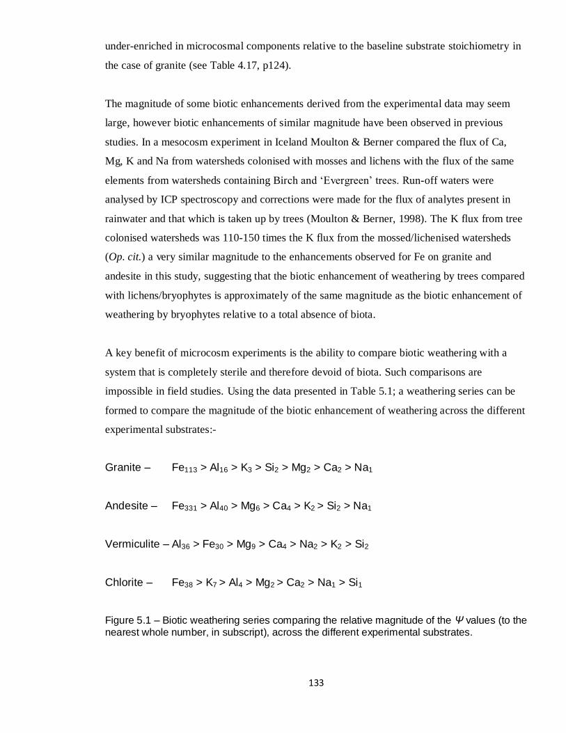
133
under-enriched in microcosmal components relative to the baseline substrate stoichiometry in
the case of granite (see Table 4.17, p124).
The magnitude of some biotic enhancements derived from the experimental data may seem
large, however biotic enhancements of similar magnitude have been observed in previous
studies. In a mesocosm experiment in Iceland Moulton & Berner compared the flux of Ca,
Mg, K and Na from watersheds colonised with mosses and lichens with the flux of the same
elements from watersheds containing Birch and „Evergreen‟ trees. Run-off waters were
analysed by ICP spectroscopy and corrections were made for the flux of analytes present in
rainwater and that which is taken up by trees (Moulton & Berner, 1998). The K flux from tree
colonised watersheds was 110-150 times the K flux from the mossed/lichenised watersheds
(Op. cit.) a very similar magnitude to the enhancements observed for Fe on granite and
andesite in this study, suggesting that the biotic enhancement of weathering by trees compared
with lichens/bryophytes is approximately of the same magnitude as the biotic enhancement of
weathering by bryophytes relative to a total absence of biota.
A key benefit of microcosm experiments is the ability to compare biotic weathering with a
system that is completely sterile and therefore devoid of biota. Such comparisons are
impossible in field studies. Using the data presented in Table 5.1; a weathering series can be
formed to compare the magnitude of the biotic enhancement of weathering across the different
experimental substrates:-
Granite – Fe113 > Al16 > K3 > Si2 > Mg2 > Ca2 > Na1
Andesite – Fe331 > Al40 > Mg6 > Ca4 > K2 > Si2 > Na1
Vermiculite – Al36 > Fe30 > Mg9 > Ca4 > Na2 > K2 > Si2
Chlorite – Fe38 > K7 > Al4 > Mg2 > Ca2 > Na1 > Si1
Figure 5.1 – Biotic weathering series comparing the relative magnitude of the Ψ values (to the nearest whole number, in subscript), across the different experimental substrates.

134
Figure 5.1 shows that the ordering of Ψ values in a highest-lowest sense is broadly similar for
granite and andesite, following the pattern:
Fe, Al… Na
The relatively lower Ψ values for vermiculite and chlorite are probably due to the fact that one
is a highly altered denudation product (vermiculite) and the other is vitreous and so less
weatherable (chlorite).
5.2 Modelling Biotic Weathering of the Earth’s Crust by Moss
Drawing on data from the different experiments presented in this thesis and the estimation of
Crowley & Baum (1991) that the area of Earth‟s land surface at 440Ma was 73.6x10⁶ km
2, it is
possible to estimate the flux of the ICP analytes in this study under different moss/land-surface
colonisation scenarios. The summary data for granite will be used for this purpose as the
stoichiometry of granite is very similar to the stoichiometry of continental crust taken as a
whole (Blatt et al., 2006). Table 5.2 below presents the different colonisation scenarios:-
Colonisation Scenario Actual Earth
surface (m2)
Whole Earth surface 7E+13
¼ Earth surface 2E+13
½ Earth Surface 4E+13
¾ Earth Surface 5E+13
Table 5.2 – Bryophyte colonisation scenarios and their corresponding Ordovician land surface area correct to 1 significant figure (calculated from Crowley & Baum (1991)).
All figures in these calculations will be rounded to 1 significant figure as there is a large
margin of error. Table 4.13, p114 shows that moss grown under optimal conditions has a mean
dry mass of 6000 mg/m2 (to 1 sig. fig.), if the value for mean dry mass of moss grown under
optimal conditions is multiplied by the data for analyte contained within the moss recovered
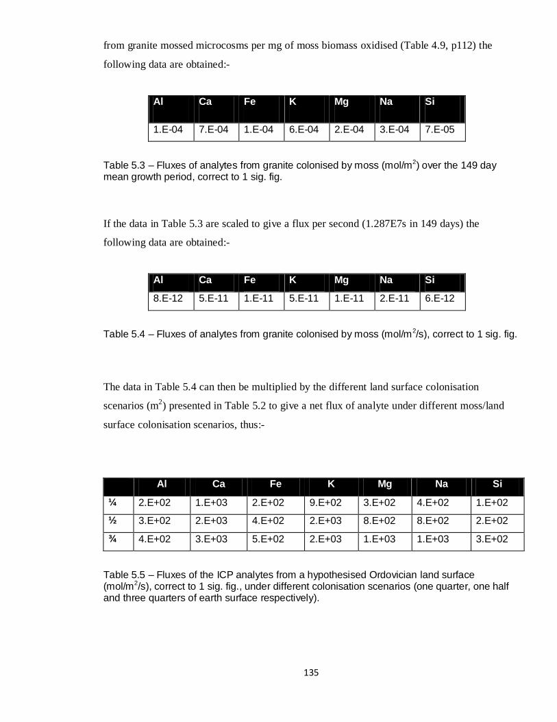
135
from granite mossed microcosms per mg of moss biomass oxidised (Table 4.9, p112) the
following data are obtained:-
Al Ca Fe K Mg Na Si
1.E-04 7.E-04 1.E-04 6.E-04 2.E-04 3.E-04 7.E-05
Table 5.3 – Fluxes of analytes from granite colonised by moss (mol/m2) over the 149 day mean growth period, correct to 1 sig. fig.
If the data in Table 5.3 are scaled to give a flux per second (1.287E7s in 149 days) the
following data are obtained:-
Al Ca Fe K Mg Na Si
8.E-12 5.E-11 1.E-11 5.E-11 1.E-11 2.E-11 6.E-12
Table 5.4 – Fluxes of analytes from granite colonised by moss (mol/m2/s), correct to 1 sig. fig.
The data in Table 5.4 can then be multiplied by the different land surface colonisation
scenarios (m2) presented in Table 5.2 to give a net flux of analyte under different moss/land
surface colonisation scenarios, thus:-
Al Ca Fe K Mg Na Si
¼ 2.E+02 1.E+03 2.E+02 9.E+02 3.E+02 4.E+02 1.E+02
½ 3.E+02 2.E+03 4.E+02 2.E+03 8.E+02 8.E+02 2.E+02
¾ 4.E+02 3.E+03 5.E+02 2.E+03 1.E+03 1.E+03 3.E+02
Table 5.5 – Fluxes of the ICP analytes from a hypothesised Ordovician land surface (mol/m2/s), correct to 1 sig. fig., under different colonisation scenarios (one quarter, one half and three quarters of earth surface respectively).
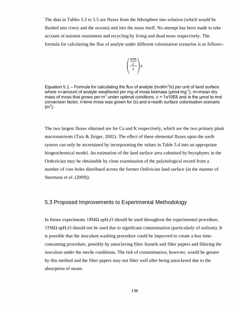
136
The data in Tables 5.3 to 5.5 are fluxes from the lithosphere into solution (which would be
flushed into rivers and the oceans) and into the moss itself. No attempt has been made to take
account of nutrient retainment and recycling by living and dead moss respectively. The
formula for calculating the flux of analyte under different colonisation scenarios is as follows:-
Equation 5.1 – Formula for calculating the flux of analyte (mol/m2/s) per unit of land surface where n=amount of analyte weathered per mg of moss biomass (μmol mg-1), m=mean dry mass of moss that grows per m2 under optimal conditons, c = 1x10E6 and is the μmol to mol conversion factor, t=time moss was grown for (s) and e=earth surface colonisation scenario (m2).
The two largest fluxes obtained are for Ca and K respectively, which are the two primary plant
macronutrients (Taiz & Zeiger, 2002). The effect of these elemental fluxes upon the earth
system can only be ascertained by incorporating the values in Table 5.4 into an appropriate
biogeochemical model. An estimation of the land surface area colonised by bryophytes in the
Ordovician may be obtainable by close examination of the palynological record from a
number of core holes distribued across the former Ordivician land surface (in the manner of
Steemans et al. (2009)).
5.3 Proposed Improvements to Experimental Methodology
In future experiments 18MΩ upH2O should be used throughout the experimental procedure,
15MΩ upH2O should not be used due to significant contamination (particularly of sodium). It
is possible that the inoculum washing procedure could be improved to create a less time-
consuming procedure, possibly by autoclaving filter funnels and filter papers and filtering the
inoculum under the sterile conditions. The risk of contamination, however, would be greater
by this method and the filter papers may not filter well after being autoclaved due to the
absorption of steam.

137
Nitric acid should be used as the ICP desorbing agent in future (instead of hydrochloric acid)
as nitric acid is cleaner (Lajunen & Peramaki, 2004). In between preparation and analysis
samples should be stored in polyethylene bottles leaving 40% volume free for expansion (as
per Parsons et al. (1984). Unfortunately, the author was unaware of both of those references
until after the experimental procedure had been completed.
5.4 Proposed Improvements to Analytical Methodology
Future experimental samples could be analysed via ICP Mass Spectrometry (ICP-MS) as
opposed to ICP-AES in order to try and reduce the number of data-points which fall between 0
and the level of precision of the instrument (non-detects). However ICP-MS analyses (whilst
having a lower limit of detection than ICP-AES analyses) are a lot more susceptible to
problematic matrix interferences, however, the author believes that analysis via ICP-MS
should still be attempted. Instrumental precision, particularly with respect to non-detects,
could be improved by the employment of the standard additions method of calibration. For
standard additions; the sample is split into ≥3 aliquots, one of these aliquots is left unaltered
and the others have an increasing, standardised amount of the experimental analytes added to
them (Lajunen & Peramaki, 2004).
The developed biomass oxidation method dissolves intracellular ions into solution in a
satisfactory and safe manner and has scope to be applied to the analysis of plant materials
other than moss. However; the interference caused by the reaction of hydrogen peroxide with
the phosphate and silicate reagents suggests that hydrogen peroxide should be precluded in
any future oxidation mix where nutrient auto analysis is planned. Mixtures of hydrogen
peroxide and nitric acid are however regarded as providing a matrix that is highly resistant to
interferences when analysed via ICP spectroscopy (Sucharova & Suchara, 2006). All „wet
chemical‟ methods used for the detection of phosphate use similar reagents to those used in
the NAA procedure (Parsons et al., 1984) and are therefore not suitable for use with the
hydrogen peroxide matrix. A solid-phase analytical method that detects phosphate at levels
>1µmol l-1
would be ideal.

138
Detection of phosphate in moss is a highly important addition that must be brought to any
future experiments in order to close the budget thoroughly for phosphate in mossed
microcosms. This is especially important given that this study appears to indicate that the
enhancement of phosphate in moss would be substantial (following the trends indicated in
Table 4.17). Given the link between increased bulk phosphate weathering and marine organic
carbon burial (Lenton, 2001), complete phosphate analysis of both the aqueous microcosmal
fractions and the moss biomass is especially needed.
Kurtosis analysis could be used to distinguish between the different types of normal
distribution rather than using a visual examination of the graphs. Instead of censoring non-
detects and substituting in a value that is half of the limit of detection: a Survival Analysis
method (such as Kaplan-Meier filtering) could be used (She, 1997). Helsel (2006) strongly
recommends against substituting non-detects for fractions of the limit of detection, but argues
that this is better than excluding or deleting non-detects as this can cause “a strong upward
bias in… means and medians.” However survival analysis techniques are not routinely used in
the environmental sciences at present and their application requires substantive specialist
knowledge that was considered beyond the scope of this study.
5.5 Proposed Further Experimental Work
Any future study of mineral weathering by biota could be greatly informed by a number of
experiments. Firstly: a large number of microcosms using each experimental substrate could
be initiated, then a small portion of these microcosms could be sampled every week and the
resulting samples kept in cold storage and then analysed in a single round. Such an experiment
would enable the plotting of a „weathering curve‟; the peak of which would inform when
maximum weathering has occurred and this could be used as the weathering period in future
experiments using that particular substrate. This assumes that there is a maximum period of
weathering beyond which moss tissue starts to die releasing weathered ions back into the
biotic aqueous solution.
Future studies into preferential weathering effects could be greatly informed if the acids
produced by mosses could be identified. Acids secreted by moss could be identified using
139
High Performance Liquid Chromatography (HPLC), this would enable validation or
falsification of the hypothesis linking moss exudates with the ionic radii of different analytes.
Whilst wild-type P. patens was used in this study there already exist a number of P. patens
mutants which are deficient in rhizines (roots), making P. patens the candidate model
bryophyte for future weathering studies (see Menand et al. (2007) for an in-depth discussion
of P. patens mutants). Similarly: thin-section and ion microprobe analysis (in the manner of
Isherwood & Street (1976)) could be used on unweathered and weathered granite clasts to
prove whether or not biotically weathered iron is derived from biotite
In addition to the control experiment using microcosms with moss inoculum but no substrate:
an experiment with microcosms containing only the filtrate could be set up in order to ensure
that the analyte present in bare microcosm fractions (see Figure 4.20, p108) is there as a result
of contamination and not due to an unknown biotic factor associated with the moss.
5.6 Concluding Statements
The temporal matching of the δ13
C excursion in the Darriwilian age of the Ordovician with the
appearance of bryophyte-like spores in the stratigraphic record (Steemans et al., 2009),
coupled with the successful demonstration by this study that mosses biotically enhance
weathering even on unlabile substrates representative of the Ordovician land surface (such as
granite) up to 113 times the level of abiotic weathering: is conducive with hypotheses linking
increased terrestrial weathering to the Ordovician glaciation (Kump et al. (1999); Sheehan
(2001); Saltzman & Young (2005)). The results of this study suggest that weathering by
bryophytes radiating across Earth‟s surface is indeed a likely cause of the Ordovician
glaciation. However such an inference cannot be made without the incorporation of the biotic
enhancement factors obtained in this study into an appropriate biogeochemical earth system
model.
The impact of the different biotic enhancement values obtained by this study after
incorporation into biogeochemical models will be highly variable. It is likely that each analyte
would be modelled separately, the impacts of biotic Al and Fe weathering compared with
weathering for the other analytes will be substantial (c.f. hundred-fold FeΨ values on granite

140
and andesite with Ψ values of ~1.5 and ~2.5 for Ca, K, Mg and Si on granite and andesite
respectively). The evidence for preferential uptake of plant macronutrients by moss (see
Figure 4.5, p84) is very interesting. It is possible that by utilsing ICP-MS as the method of
analysis in future experiments appearences of this effect could be better resolved. If ICP-MS
were used in tandem with HPLC characterisation of moss exudates (see previous section) a
much greater understanding of how mosses (and plants in general) weather minerals in order
to meet their nutritional requirements would be obtained.
The strong enrichments of ions into the control aqueous fractions in micrococosms where no
biota was present over the baseline stoichiometry of the substrates is indicative that abiotic
weathering plays a strong role in making plant macronutrients available and is likely to have
been a key mechanism facilitating the evolution of plant life on Earth by making
physiologically useful compounds available. The fact that Al was commonly the analyte with
the second highest biotic enhancement value is interesting. Al was frequently found to
accumulate in moss tissue to levels up to 0.2μmol in moss that appeared to be thriving. This
contrasts with the view of aluminium as an analyte with a low toxic threshold in plants, and
lends weight to the findings of Marschner (1995) cit. in Taiz & Zeiger (2002) that low levels
of aluminium are beneficial to plant growth.
The fact that Fe was the most biotically enhanced analyte on all substrates except vermiculite
and that the biotic enhancements of Fe were always of a very high magnitude compared to the
other analytes is very interesting. An issue pertinent to the Ordovician glaciation is that its
onset occurred when atmospheric pCO2 was 10-18x PAL (Yapp & Poths (1992) and Pope &
Steffen (2003)). Central to this issue is what caused atmospheric pCO2 to decline to the levels
necessary to trigger the glaciation? Kump & Arthur (1999) suggest a level of 10x PAL as
sufficient.
This study hints at a possible explanation for the decrease in atmospheric pCO2 in the form of
an increase in Fe export to the oceans via rivers as a result of increased biotic terrestrial
weathering. Cooper et al. (1996) found that adding (or „fertilising‟) Fe-deplete regions of the
ocean (known as „High-Nitrate Low-Chlorophyll‟ or „HNLC‟ regions) with Fe to
concentrations in the seawater as low as 2nM led to a 60% reduction in the ocean to
atmosphere CO2(g) flux as a result of the increasing productivity of marine phytoplankton. This

141
60% reduction equates to 2850 tonnes of carbon over the 30x25km test area over the 17 day
experiment (Op. cit.). This carbon is eventually sequestered in the deep ocean as the
phytoplankton die and form a part of the Particulate Organic Carbon (POC) flux from the
surface to the deep ocean (also known as the „Biological Pump‟) (Op. cit. and Watson et al.
(2000). Watson et al. demonstrated that accumulation of Fe in dust in the Vostok ice core
matches decreases in atmospheric pCO2 found in the same ice core (indicating that an increase
in aeolian deposition of Fe leads to a decrease in atmospheric pCO2). Watson et al. proved
empirically that these factors are linked to Fe-fertilisation of phytoplankton in HNLC regions
of the oceans using an ocean-atmosphere carbon-cycle box model. The atmospheric pCO2
output of the model closely matches the profile of atmospheric pCO2 obtained from the Vostok
ice core where ΔpCO2 <40ppmv and aeolian deposition of Fe is altered to match the levels in
the ice core over time (Op. cit.).
To conclude: the author‟s hope is that this study will be viewed as a good example of what can
successfully be achieved when an Earth systems science approach is adopted and
collaborations are formed between scientists from seemingly disparate disciplines (e.g. as in
this study; geochemists and plant scientists). More importantly; the author hopes that this
thesis will prompt others to study the effects biota have upon mineral weathering and that the
resulting data obtained from these studies will improve understanding of the effects of mineral
weathering as an input to global biogeochemical cycles and that this will lead to an improved
understanding of the long-term carbon cycle and reduce the error currently associated with
some parameters in biogeochemical models.

142
6: List of References
Aghamiri, R., & Schwartzman, D. W. (2002). Weathering rates of bedrock by lichens: a mini watershed study. Chemical Geology, 188(3-4), 249-259. Andrews, J. E.,Brimblecombe, P.,Jickells, T. D., & Reid, B. (2004). An Introduction To Environmental Chemistry (2nd ed.). Oxford: Blackwell. Baars, C.,Jones, T. H., & Edwards, D. (2008). Microcosm studies of the role of land plants in elevating soil carbon dioxide and chemical weathering. Global Biogeochemical Cycles, 22(3). Banwell, C. N. (1983). Fundamentals of Molecular Spectroscopy (Vol. 3rd Ed.). Maidenhead: Mc-Graw Hill Education. Barry, R. G., & Chorley, R. J. (2003). Atmosphere, Weather And Climate. London: Routledge. Berner, R. A. (1992). Weathering, plants, and the long-term carbon cycle. Geochimica et Cosmochimica Acta, 56(8), 3225-3231. Berner, R. A. (1998). The carbon cycle and CO(2) over Phanerozoic time: the role of land plants. Philosophical Transactions of The Royal Society of London (B), 353, 75-82. Berner, R. A. (2004). The Phanerozoic Carbon Cycle: CO2 and O2. Oxford: Oxford University Press. Blakey, R. (2009). Late Ordovician (450Ma). Retrieved 16 December 2009, from http://jan.ucc.nau.edu/~rcb7/450moll.jpg Blatt, H.,Tracy, R. J., & Owens, B. E. (2006). Petrology: Igneous, Sedimentary and Metamorphic (3rd Edition ed.). Basingstoke: W.H. Freeman and Company. Brenchley, P. J.,Marshall, J. D.,Carden, G. A. F.,Robertson, D. B. R.,Long, D. G. F.,Meidla, T.,Hints, L., & Anderson, T. F. (1994). Bathymetric and isotopic evidence for a short-lived Late Ordovician glaciation in a greenhouse period. Geology, 22(4), 295-298. Cooper, D. J.,Watson, A. J., & Nightingale, P. D. (1996). Large decrease in ocean-surface CO2 fugacity in response to in situ iron fertilization. Nature, 383(6600), 511-513. Crouch, M. J. C. (2007). On the Biotic Enhancement of Weathering by Lichens. University of East Anglia, Norwich. Crowley, T. J., & Baum, S. K. (1991). Toward reconciliation of late Ordovician (~440 Ma) glaciation with very high CO2 levels. Journal of Geophysical Research, 96(D12). Deer, W. A.,Howie, R. A., & Zussman, J. (1966). An Introduction to the Rock Forming Minerals. London: Longman. Fairchild, I. J., & Kennedy, M. J. (2007). Neoproterozoic glaciation in the Earth System. Journal of the Geological Society, London, 164, 895-921.

143
Ford Cochran, M., & Berner, R. A. (1996). Promotion of chemical weathering by higher plants: field observations on Hawaiian basalts. Chemical Geology, 132(1-4), 71-77. Gibbs, M. T.,Barron, E. J., & Kump, L. R. (1997). An atmospheric pCO(2) threshold for glaciation in the Late Ordovician. Geology, 25(5), 447-450. Gradstein, F. M.,Ogg, J. G., & Smith, A. G. (2004). A Geologic Timescale 2004. Cambridge: Cambridge University Press. Graham, R. C.,Rossi, A. M., & Hubbert, K. R. (2010). Rock to regolith conversion: Producing hospitable substrates for terrestrial ecosystems. GSA Today, 20(2), 4-9. Hasebe, M. (2009). The Life-Cycle of Physcomitrella patens, from http://moss.nibb.ac.jp/images/life2.gif Hatcher, W. H., & MacLauchlan, D. W. (1938). The Conductivity and Reactivity of Nitric Acid and Hydrogen Peroxide Mixtures. Canadian Journal of Research, 16B. Hazen, R. M. (2009). Animal, vegetable: both made mineral. New Scientist, 14. Helsel, D. R. (2006). Fabricating data: How substituting values for nondetects can ruin results, and what can be done about it. Chemosphere, 65(11), 2434-2439. Hoffland, E.,Kuyper, T. W.,Wallander, H.,Plassard, C.,Gorbushina, A. A.,Haselwandter, K.,Holmstrom, S.,Landeweert, R.,Lundstrom, U. S.,Rosling, A.,Sen, R.,Smits, M. M.,van Hees, P. A., & van Breemen, N. (2004). The role of fungi in weathering. Frontiers in Ecology and the Environment, 2(5), 258-264. Imperial. (2010). Imperial College, London: Database of Ionic Radii. Retrieved 24th March 2010, 2010, from http://abulafia.mt.ic.ac.uk/shannon/ptable.php Isherwood, D., & Street, A. (1976). Biotite-induced grussification of the Boulder Creek Granodiorite, Boulder County, Colrado. Geological Society of America Bulletin, 87, 366-370. Jackson, T. A., & Keller, W. D. (1970). A comparative study of the role of lichens and "inorganic" processes in the chemical weathering of Recent Hawaiian lava flows. American Journal of Science, 269(5), 446-466. Kump, L. R., & Arthur, M. A. (1999). Interpreting carbon-isotope excursions: carbonates and organic matter. Chemical Geology, 161(1-3), 181-198. Kump, L. R.,Arthur, M. A.,Patzkowsky, M. E.,Gibbs, M. T.,Pinkus, D. S., & Sheehan, P. M. (1999). A weathering hypothesis for glaciation at high atmospheric pCO(2) during the Late Ordovician. Palaeogeography Palaeoclimatology Palaeoecology, 152(1-2), 173-187. Lajunen, & Peramaki. (2004). Spectrochemical Analysis by Atomic Absorption and Emission (2nd ed.). London: Royal Society of Chemistry. Lenton, T. M. (2001). The role of land plants, phosphorus weathering and fire in the rise and regulation of atmospheric oxygen. Global Change Biology, 7(6), 613-629.

144
Lenton, T. M., & Watson, A. J. (2004). Biotic enhancement of weathering, atmospheric oxygen and carbon dioxide in the Neoproterozoic. Geophysical Research Letters, 31(5), 5. Lewis, D. G., & Quirk, J. P. (1967). Phosphate diffusion in soil and uptake by plants P-31 movement and uptake by plants as indicated by P-32 autoradiography. Plant and Soil, 26(3), 445-&. Libes, S. M. (1992). An Introduction To Marine Biogeochemistry. New York, NY, USA.: John Wiley & Sons, Inc. Liss, P. S., & Spencer, C. P. (1969). An investigation of some methods used for determination of silicate in sea water. Journal of the Marine Biological Association of the United Kingdom, 49(3), 589. Lovelock, J. E. (1979). Gaia: A New Look At Life On Earth. Oxford: Oxford University Press. Mackenzie, W. S., & Adams, A. E. (1994). A Colour Atlas of Rocks and Minerals in Thin Section. London: Manson Publishing Ltd. Marienfeld, J. R.,Reski, R.,Friese, C., & Abel, W. O. (1989). Isolation of Nuclear, Chloroplast and Mitochondrial DNA from the Moss Physcomitrella patens. Plant Science, 61, 235-244. Menand, B.,Yi, K. K.,Jouannic, S.,Hoffmann, L.,Ryan, E.,Linstead, P.,Schaefer, D. G., & Dolan, L. (2007). An ancient mechanism controls the development of cells with a rooting function in land plants. Science, 316(5830), 1477-1480. Moulton, K. L., & Berner, R. A. (1998). Quantification of the effect of plants on weathering: Studies in Iceland. Geology, 26(10), 895-898. Pallant, J. (2007). SPSS Survival Manual (3rd Ed.). Maidenhead.: McGraw-Hill/Open University Press. Parsons, T.,Maita, V., & Lalli, C. (1984). A manual of chemical and biological methods for seawater analysis. Oxford: Pergamon. Pope, M. C., & Steffen, J. B. (2003). Widespread, prolonged late Middle to Late Ordovician upwelling in North America: A proxy record of glaciation?: Correction. Geology, 31(7), 656-656. Reski, R., & Cove, D. J. (2004). Physcomitrella patens. Current biology : CB, 14(7), R261-262. Saltzman, M. R., & Young, S. A. (2005). Long-lived glaciation in the Late Ordovician? Isotopic and sequence-stratigraphic evidence from western Laurentia. Geology, 33(2), 109-112. Schaefer, D. G. (2002). A new moss genetics: Targeted mutagenesis in Physcomitrella patens, Annual Review of Plant Biology (Vol. 53, pp. 477-501). Schwartzman, D. W. (2000). Life, Temperature and the Earth: The Self-Organizing Biosphere. New York, NY, USA.: Columbia University Press. She, N. (1997). Analyzing censored water quality data using a non-parametric approach. Journal of the American Water Resources Association, 33(3), 615-624. Sheehan, P. M. (2001). The Late Ordovician Mass Extinction. Annual Review of Earth and Planetary Sciences, 29, 331-364.

145
Spokes, L. J.,Yeatman, S. G.,Cornell, S. E., & Jickells, T. D. (2000). Nitrogen deposition to the eastern Atlantic Ocean. The importance of south-easterly flow. Tellus B, 52(1), 37-49. Steemans, P.,Herisse, A. L.,Melvin, J.,Miller, M. A.,Paris, F.,Verniers, J., & Wellman, C. H. (2009). Origin and Radiation of the Earliest Vascular Land Plants. Science, 324(5925), 353-. Sterner, R. W., & Elser, J. J. (2002). Ecological stoichiometry: the biology of elements from molecules to the biosphere. Woodstock: Princeton University Press. Street-Perrott, F. A., & Barker, P. A. (2008). Biogenic silica: a neglected component of the coupled global continental biogeochemical cycles of carbon and silicon. Earth Surface Processes and Landforms, 33, 1436-1457. Sucharova, J., & Suchara, I. (2006). Determination of 36 elements in plant reference materials with different Si contents by inductively coupled plasma mass spectrometry: Comparison of microwave digestions assisted by three types of digestion mixtures. Analytica Chimica Acta, 576(2), 163-176. Taiz, L., & Zeiger, E. (2002). Plant Physiology (3rd Ed.) (Vol. Sunderland, MA, USA.): Sinauer Associates Inc. Taylor, D. J.,Green, N. P. O., & Stout, G. W. (Eds.). (1997). Biological Science 1 (3rd ed.). Cambridge: Cambridge University Press. TVA. (2010). The Vermiculite Association: Properties. Retrieved 15/01/2010, from http://www.vermiculite.org/Properties6.html UBC. (2010). Bryophytes of Stanley Park: Bryophyte Evolution. Retrieved 7/1/2010, 2010, from http://www.botany.ubc.ca/bryophyte/stanleypark/evolution.htm UNU. (1992). The Evolving Gaia Theory: Paper presented at The United Nations University Lectures, from http://www.unu.edu/unupress/lecture1.html USGS. (2003). The Highlands Province: The Taconic Orogeny. Retrieved 6/1/2010, 2010, from http://3dparks.wr.usgs.gov/nyc/highlands/highlands.html Wainwright. (2010). geology. Retrieved 15/01/2010, from http://www.wainwright.co.uk/geology.php Watson, A. J.,Bakker, D. C. E.,Ridgwell, A. J.,Boyd, P. W., & Law, C. S. (2000). Effect of iron supply on Southern Ocean CO2 uptake and implications for glacial atmospheric CO2. Nature, 407(6805), 730-733. Wellman, C. H.,Osterloff, P. L., & Mohiuddin, U. (2003). Fragments of the earliest land plants. Nature, 425, 282-285. White, A. F., & Brantley, S. L. (2003). The effect of time on the weathering of silicate minerals: why do weathering rates differ in the laboratory and field? Chemical Geology, 202(3-4), 479-506. Yapp, C. J., & Poths, H. (1992). Ancient atmospheric CO(2) pressures inferred from natural goethites. Nature, 355, 342-344.

146
Zhang, J. Z.,Fischer, C. J., & Ortner, P. B. (1999). Laboratory glassware as a contaminant in silicate analysis of natural water samples. Water Research, 33(12), 2879-2883.

147
Index to Appendices
Section Title/Sub-Section Start
Page
Appendix i Further Methodology
i.i – Method Development 148
i.ii – Laboratory Protocols 150
i.iii – Mathematical Operations 153
Appendix ii Blank Analysis Data
ii.i – Contamination in experimental waters 155
ii.ii – Contamination during inoculum preparation
stages
157
ii.iii – Substrate wash analysis 159
ii.iv – Contamination from heated plasticware 161
ii.v – upH2O Blanks – Frequency Distribution Analyses 162
ii.vi – Inoculum at Initial Conditions – Frequency
Distribution Analyses
165
ii.vii – Na in Granite Aggregated Dataset – Frequency
Distribution Analysis
169
Appendix iii Graphs of Data from Individual Experiments
iii.i – Granite Experiments 170
iii.ii – 28/11/08 Andesite Experiment 176
iii.iii – Vermiculite Experiments 177
iii.iv – 24/6/08 Chlorite Experiment 179
Appendix iv Data
iv.i – Mann-Whitney U Test 180
iv.ii – T-test for Independent Samples 182
iv.iii – XRF Data: Petrology of Substrates 184
iv.iv – Data Summaries 185
iv.v – Amounts of NAA analytes in Aqueous
Microcosm Components
191
iv.vi – Amounts of ICP Analytes in Aqueous
Microcosm Components
-
iv.vii - Amounts of ICP Analytes in Oxidised Moss -
iv.viii – Desorbing agent blank data -
iv.ix – upH2O blank data -
iv.x – Filtrate at initial conditions data -
iv.xi – Nitric acid and hydrogen peroxide blank data -
iv.xii – Inoculum at initial conditions data -

148
Appendix i – Further Methodology
i.i Method Development
i.i.i Pilot Oxidation Experiments using Arabidopsis Tissue
A small amount of tissue from the flowering plant Arabidopsis thaliana was added to five
centrifuge tubes. 10ml of 10% Nitric Acid was then added to these tubes and the tubes were
vortexed for 10 seconds before 10ml of 10% Hydrogen Peroxide was added and the tubes
vortexed again for 10 seconds. The tubes were then incubated in a heat block at 40°C for one
hour; the tubes were shaken by hand periodically. The entire procedure was conducted in a
fume cabinet with the sash ¾ lowered, and personal protective equipment was worn at all
times.
After one hour the plant tissue did not visibly appear to have degraded beyond the fact that the
chlorophyll had been released, turning the solution a pale green. I therefore increased the
concentrations of the Nitric Acid and the Hydrogen Peroxide to 20% and repeated the
procedure: this caused the plant tissue to turn more translucent and more chlorophyll to be
released, but did not result in the complete oxidation of tissue required. I then increased the
concentrations of Nitric Acid and the Hydrogen Peroxide to 30%, at these concentrations the
tissue began to degrade.
Increasing the concentrations of the oxidation mix still further would have been ill-advised
because Hydrogen Peroxide becomes unstable at concentrations >32% (Hatcher &
MacLauchlan, 1938), it was therefore decided to increase the incubation temperature in a
series of experiments to 50°C, 60°C and finally 70°C. At 70°C the reaction was found to
proceed so well that the reaction time could be halved to 30 minutes for new moss biomass
samples. The experiment was then repeated with moss inoculum and found to work
satisfactorily.

149
i.i.ii Initial Microcosm Water Sampling Methods
i.i.ii.i Method 1
150μl of the aqueous solution within the microcosm was pipetted off into a new centrifuge
tube using a 1000μl pipette and tip, a new tip being used for each microcosm to prevent
contamination. In order to make up the resulting solution to the minimum volume for ICP
analysis; 3.45ml of upH2O was added to each centrifuge tube using a 5ml pipette and tip, and
the tubes were lightly shaken to homogenise the contents. On addition of 400μl of desorbing
agent a resulting solution of 4000μl was produced for ICP analysis.
i.i.ii.ii Method 2
Sampling Method 2 is identical to Method 1 with the following exceptions:-
1. 200μl of aqueous solution was pipetted off each microcosm.
2. 3720μl of upH2O was added to each centrifuge tube.
3. 80μl of desorbing agent was added to each centrifuge tube.

150
i.ii Laboratory Protocols
i.ii.i Substrate Washing Protocol
1. In a 1L glass beaker add substrate to 400ml line.
2. Add 15MΩ upH2O to 1L line.
3. Mix with a clean spoon and stand for 10mins.
4. After 10mins pour suspension through a sieve (retaining 50ml for analysis).
5. Rinse spoon, beaker and sieve clean of material with dH2O.
6. Add substrate from sieve back to beaker and repeat stages 2-6 without standing for
10mins.
7. Repeat 6.
8. Add substrate from sieve, add 18MΩ upH2O to 1L line and repeat stage 6.
9. Place substrate into a clean 500ml glass beaker. Place two sheets of aluminium foil
over the top of the beaker and seal around the rim.
10. Heat sterilise.
i.ii.ii Knop’s Plates Preparation Protocol
The media was prepared and stored in an oven at 55°C for no more than three days prior to
use. Plates were made by adding 10ml of molten Knop‟s media to sterile plastic petri dishes
and allowing the media to solidify and cool. Circular cellulose discs31
80mm in diameter were
then placed on top of the media using forceps, without these discs the moss grows into the
media and is very difficult to remove. The lids were then placed on top of the plates and the
plates were placed in a growth room for five days. After five days the moss was collected from
each plate using a sterilised metal spatula, the moss from each plate being placed into a 5ml
bijou jar of sterile water.
31 Custom manufactured by: A.A. Packaging Ltd., Preston, Lancashire, UK.

151
i.ii.iii Nutrient Auto Analyser (NAA) Protocols
Reagent Feedstock Chemicals
Phosphate 1 125ml of 280ml/l concentrated Sulphuric Acid
3.0g Ammonium Molybdate Tetrahydrate
0.115g Potassium Antimonyl Tartrate†
0.1g Sodium Dodecyl Sulfate‡
Phosphate 2 5.5g Ascorbic Acid
30ml Propanone
0.1g Sodium Dodecyl Sulfate
Silicate 1 10.0g Ammonium Molybdate Tetrahydrate
0.25g Sodium Dodecyl Sulfate
Silicate 2 22.0g Oxalic acid‡
Silicate 3 20.0g Ascorbic acid‡
Feedstock chemicals used to produce the Nutrient Auto Analyser reagents. All chemicals were added to a 500ml volumetric flask and made up to volume with upH2O. Chemicals were supplied by Fisher Chemical
32 unless otherwise stated:-
†Supplied by: BDH/Merck.
33
‡Supplied by: Sigma–Aldrich.34
32 Fisher Scientific UK Ltd, Loughborough, Leicestershire, LE11 5RG, UK. 33 Merck Chemicals Ltd., Hull, HU1 1UY, UK. 34 Sigma-Aldrich Company Ltd., Dorset, UK.

152
i.ii.iv XRF Protocol
1: Wipe disc mill pans and fusion bead crucibles with propan-2-ol. Rinse with distilled water.
2: Place crucibles onto Mettler Toledo XS205 (Dual Range) 5.d.p. balance (d=0.01mg).
Ensure sides and top are fully closed. When figures stop cycling tare balance.
3: Weigh out 7.60000g of Lithium Borate flux (as accurately as possible).
4: Add 0.40000g of milled rock sample to the flux, giving a flux + sample as close to
8.00000g as possible.
5: Stir mixture using a propan-2-ol cleaned spatula. Place platinum crucibles in fusion bead
machine (see next section).
6: Allow resulting beads to cool. Label them on the larger side.
7: Analyse on Bruker XRF machine.

153
i.ii.v Phoenix Fusion Bead Machine Protocol
1: Turn on butane cylinder at regulator. Turn on oxygen cylinder.
2: Ensure you have pressure of >4 bar.
3: Switch on „Phoenix‟ machine set to the following programme:-
Pre-Melt 240s
Melt 180s
Swirl 200s
Pour 20s
Cool delay 10s
Pre-cool 40s
Total cool 240s
4: Switch on burners beneath the crucibles. Press down start button for >5s.
i.iii Mathematical Operations
i.iii.i Standard Deviation
The standard deviation was calculated using Microsoft Excel internal „stdev‟ operation. Excel
calculates the standard deviation using the following formula:-
Where: χ = sample mean and n = sample size.

154
i.iii.ii Standard Error
The standard error of the mean was calculated using the standard deviation from Excel above
and the following formula:-
Where: σ = standard deviation and n = sample size.

155
Appendix ii – Blank Analysis Data
ii.i Contamination in experimental waters
ii.i.i Ultra pure waters
Graph showing contamination in 15MΩ and 18MΩ Ultra Pure Waters, note the substantially
higher levels of contamination (8.9-62.3 times, depending on analyte) in 15MΩ upH2O relative
to 18MΩ upH2O. Error bars represent 1σ 15MΩ n=10, 18MΩ n=98. NB the analysis shown
above was conducted after all experiments had been completed and could not therefore be
used to inform experimental methods.
0.0
2.0
4.0
6.0
8.0
10.0
12.0
Al Ca Fe K Mg Na Si
Co
ncen
trati
on
of
an
aly
te (
µm
ol
l-1)
15MΩ
18MΩ

156
ii.i.ii Contamination in sterile water
Graph showing contamination in sterile (autoclaved 18MΩ upH2O) relative to non-autoclaved
18MΩ upH2O (Sterile n=5, 18MΩ n=98). NB Initial pilot studies used only three analytes (Al,
Fe and Si) for simplicity.
The data shown above were unexpected: the steam generator used to autoclave items generates
steam using dH2O rather than upH2O. As the lids of the bijou jars have to be kept loosened by
¼ turn in order to stop the jars from imploding at high pressure, it was expected that dH2O
would enter the upH2O in the vapour phase thus contaminating the upH2O. The graph appears
to be weakly demonstrating the opposite for Al and Fe. It is important to note that there are
only data for three analytes and that the data for the sterile water consists of five pseudo-
replicates (five sub-samples of one sample) taken on one day, whereas the upH2O dataset
represents 98 pseudo-replicates taken over 23 days. The upH2O dataset is therefore much more
robust than the sterile water dataset. The effects of contamination are mitigated by a rigorous
blank correction procedure.
0.0
0.1
0.2
0.3
0.4
0.5
0.6
Al Fe Si
Co
ncen
trati
on
of
an
aly
te (
μm
ol
l-1)
Sterile
18MΩ

157
ii.ii Contamination during inoculum preparation stages
Contamination in the 1st and 2nd sterile water washes (‘1’ and ‘2’) during the preparation of the
29/7/09 inoculum). ‘3’ is the final wash in upH2O that forms the filtrate that is added to control
microcosms.
0
50
100
150
200
250
1 2 3
Am
ou
nt
of
an
aly
te (
µm
ol)
Inoculum 'Wash'
Al
Ca
Fe
K
Mg
Na
Si
Log. (Ca)
Linear (K)
Log. (Mg)
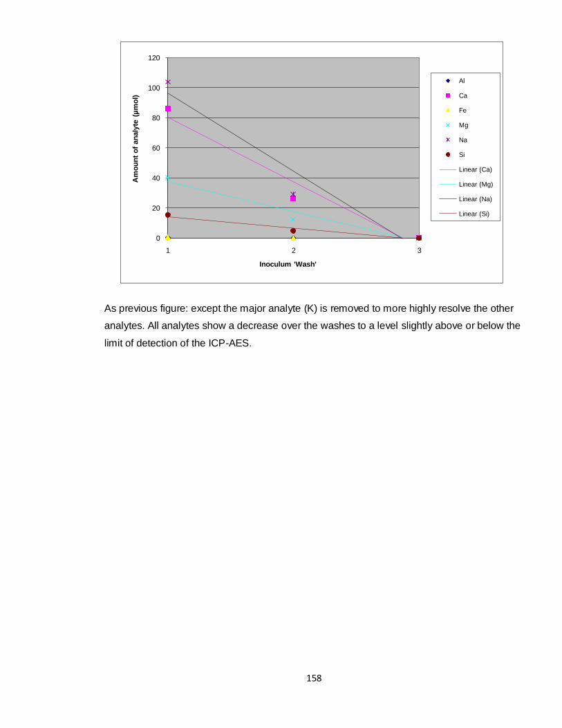
158
As previous figure: except the major analyte (K) is removed to more highly resolve the other
analytes. All analytes show a decrease over the washes to a level slightly above or below the
limit of detection of the ICP-AES.
0
20
40
60
80
100
120
1 2 3
Am
ou
nt
of
an
aly
te (
µm
ol)
Inoculum 'Wash'
Al
Ca
Fe
Mg
Na
Si
Linear (Ca)
Linear (Mg)
Linear (Na)
Linear (Si)

159
ii.iii Substrate wash analysis
The trends for the substrate washes were mainly negative with linear or logarithmic („curved‟)
trend-lines. 3 out of 14 datasets formed asymmetric distributions (i.e. the final wash contained
a higher amount of an analyte than the first wash). The figures below demonstrate the types of
distribution observed in the substrate wash datasets:-
4/2/09 Vermiculite wash data, all analytes exhibiting logarithmic negative correlations. Analysis by ICP-AES.
4/2/09 Andesite wash data, all analytes exhibiting two order asymmetrical distributions with many analytes exhibiting a higher amount in the final wash than the first wash.
0
10
20
30
40
50
60
70
80
90
100
1 2 3 4
Am
ou
nt
of
an
aly
te (
µm
ol)
Substrate Wash
Al
Ca
Fe
K
Mg
Na
Si
Log. (Ca)
Log. (K)
Log. (Mg)
Log. (Na)
Log. (Si)
0
50
100
150
200
250
300
350
400
1 2 3 4
Am
ou
nt
of
an
aly
te (
µm
ol)
Substrate Wash
Al
Ca
Fe
K
Mg
Na
Si
Poly. (Ca)
Poly. (Mg)
Poly. (Na)
Poly. (Si)

160
The negative, curved trend-lines exhibited by all analytes in the 4/2/09 vermiculite wash data
are to be expected; the more a substrate was washed with upH2O the more adsorbed ions and
deposited contaminants were removed from the mineral surface. This affect was observed
whilst washing the mineral/rock; the solution resulting from the first wash was frequently
extremely turbid (and several filters were clogged preparing the sample for analysis. The
turbidity of each wash decreased until the final wash, which was normally relatively
transparent to light.
The asymmetrical distributions may be explained by the fact that the 15MΩ upH2O contained
more ions such as bicarbonate (HCO3-) and carbonate (CO3
2-) than the „cleaner‟ 18MΩ
upH2O. HCO3- and CO3
2- are the main ions responsible for alkalinity, buffering acidity in
natural waters (Andrews et al., 2004), therefore 18MΩ upH2O will be more acidic than 15MΩ
upH2O and as such would have been more able to release ions adsorbed onto the rock surface.
Furthermore; the increasing use of glassware across the rock wash procedure could explain
any increase in Si contamination in the final washes as Si is leached from the silica glassware
(Zhang et al., 1999). The high amounts of analytes in the final wash results could also, simply,
be experimental artefacts.

161
ii.iv – Contamination from heated plasticware
Contamination in upH2O heated in plastic centrifuge tubes (n=5) relative to unheated upH2O
(n=4). 1σ error bars overlap for all analytes indicating that any leaching effect from plastic is
statistically insignificant.
0
0.1
0.2
0.3
0.4
0.5
0.6
Al Ca Fe K Mg Na Si
Mean
co
ncen
trati
on
of
an
aly
te (
μm
ol
l-1)
Unheated
Heated

162
ii.v upH2O Blanks – Frequency Distribution Analyses

163

164

165
ii.vi Inoculum at initial conditions – Frequency Distribution Analyses

166
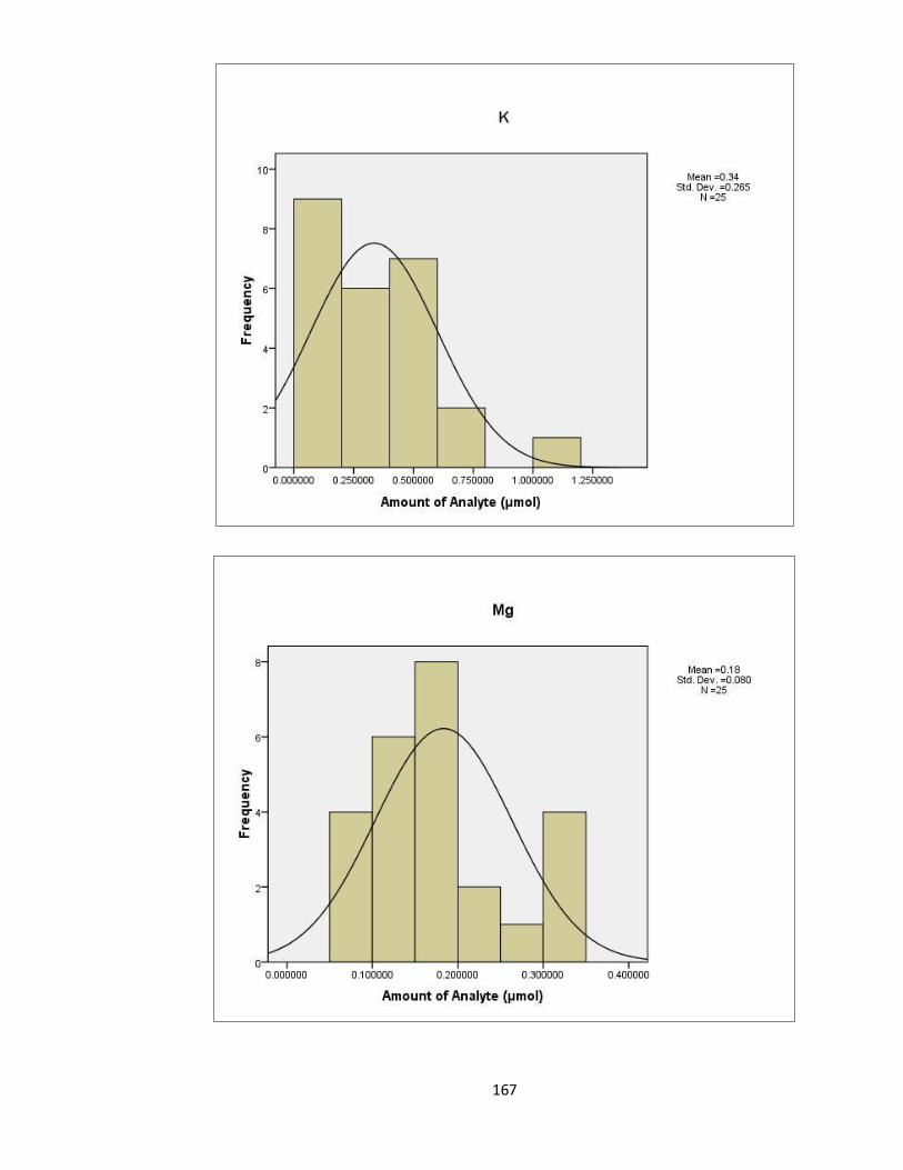
167

168
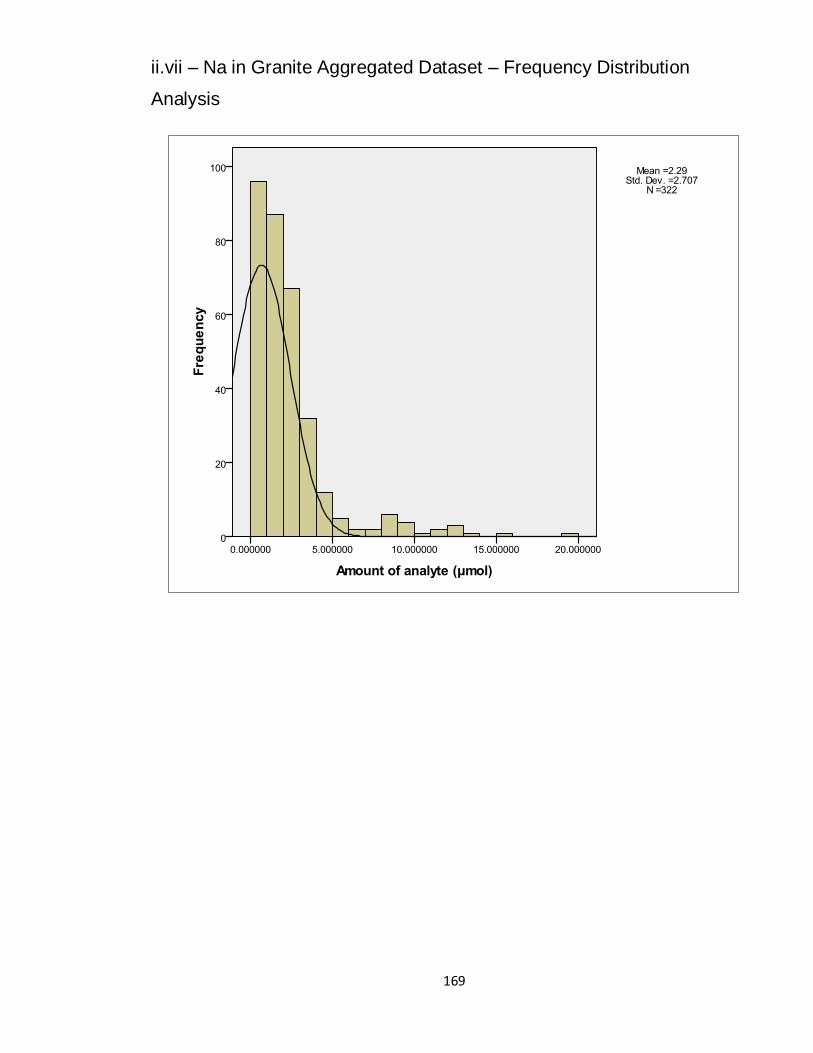
169
ii.vii – Na in Granite Aggregated Dataset – Frequency Distribution
Analysis

170
Appendix iii – Graphs of Data from Individual Experiments
iii.i Granite Experiments
Below are weathering data (normalised to abiotic weathering) for the individual granite
experiments that are not presented in the main body of the text.
iii.i.i 30/4/08 Granite Experiment

171
iii.i.ii 2/9/08 Granite Experiment

172
iii.i.iii 19/12/08 Granite Experiment

173
iii.i.iv 30/7/09 Granite Experiment

174
iii.i.v 30/4/08 Granite Experiment – NAA Data
0.0
0.1
0.2
0.3
0.4
0.5
0.6
SiO(4) PO(4)
Mean
am
ou
nt
of
an
aly
te (
µm
ol)
Abiotic Weathering
Total Aqueous
Weathering
iii.i.vi 24/6/08 Granite Experiment – NAA Data
0.00
0.05
0.10
0.15
0.20
0.25
0.30
0.35
0.40
0.45
SiO(4)
Mean
am
ou
nt
of
silic
ate
(µ
mo
l)
Abiotic Weathering
Total AqueousWeathering
NB No phosphate was detectable in either the control microcosm aqueous fractions or the mossed microcosm aqueous fractions.

175
iii.i.vii 2/9/08 Granite Experiment – NAA Data
0.00
0.05
0.10
0.15
0.20
SiO(4) PO(4)
Mea
n a
mo
un
t o
f a
na
lyte
(µ
mo
l)
Abiotic Weathering
Total AqueousWeathering

176
iii.ii 28/11/08 Andesite Experiment
The only andesite experiment that is not presented in the main body of the text is the 28/11/08
experiment. The weathering data (normalised to abiotic weathering) are presented below:-

177
iii.iii Vermiculite experiments
Only the aggregated weathering data for vermiculite is presented in the main body of this
thesis. Both the 14/2/08 and 17/2/09 individual experimental datasets are presented in
graphical format below (normalised to abiotic weathering):-
iii.iii.i 14/2/08 Vermiculite Data

178
iii.iii.ii 17/2/09 Vermiculite Data

179
iii.iv 24/6/08 Chlorite experiment
The ICP data for the 24/6/08 chlorite is presented in the main body of the text. The statistically
insignificant NAA data are presented below:-
0
0.05
0.1
0.15
0.2
0.25
0.3
SiO(4) PO(4)
Mean
am
ou
nt
of
an
aly
te (
μm
ol)
Abiotic Weathering
Total AqueousWeathering

180
Appendix iv – Data
iv.i Mann-Whitney U Test
Below are presented the SPSS outputs for the Mann-Whitney U test. „Asymp. Sig. (2-tailed)‟
is the P value for the test to three decimal places.
iv.i.i Granite Aggregated Data
Granite – Wa vs. Wtot
Al Ca Fe K Mg Na Si
Mann-Whitney U 63.000 1497.000 3.000 403.000 1295.000 1764.000 1279.000
Wilcoxon W 3066.000 4500.000 3006.000 3406.000 4298.000 3475.000 4282.000
Z -9.646 -3.272 -10.308 -8.135 -4.169 -2.085 -4.240
Asymp. Sig. (2-tailed) .000 .001 .000 .000 .000 .037 .000
Granite – Wa vs. Wb
Al Ca Fe K Mg Na Si SiO4 PO4
Mann-Whitney U 1609.000 1409.000 2161.000 2129.000 1495.500 2032.000 2436.500 439.000 319.000
Wilcoxon W 4612.000 4037.000 5164.000 4757.000 4123.500 4660.000 5439.500 1000.000 880.000
Z -4.418 -5.178 -2.728 -2.443 -4.849 -2.811 -1.274 -.976 -3.098
Asymp. Sig. (2-
tailed)
.000 .000 .006 .015 .000 .005 .203 .329 .002

181
iv.i.ii Andesite Aggregated Data
Andesite – Wa vs. Wtot
Al Ca Fe K Mg Na Si
Mann-Whitney U 19.000 205.000 .000 296.000 102.000 704.000 130.000
Wilcoxon W 722.000 908.000 703.000 999.000 805.000 1607.000 833.000
Z -7.447 -5.620 -7.863 -4.726 -6.632 -.717 -6.357
Asymp. Sig. (2-tailed) .000 .000 .000 .000 .000 .473 .000
Andesite – Wa vs. Wb
Al Ca Fe K Mg Na Si
Mann-Whitney U 654.500 557.000 640.500 734.000 755.000 628.000 482.000
Wilcoxon W 1515.500 1260.000 1343.500 1595.000 1458.000 1489.000 1343.000
Z -1.041 -2.016 -1.546 -.245 -.035 -1.306 -2.767
Asymp. Sig. (2-tailed) .298 .044 .122 .806 .972 .192 .006
iv.i.iii Vermiculite Aggregated Data
Vermiculite – Wa vs. Wtot
Al Ca Fe K Mg Na Si
Mann-Whitney U 5.000 47.000 6.000 139.000 2.000 185.000 269.000
Wilcoxon W 671.000 713.000 672.000 805.000 668.000 851.000 935.000
Z -7.294 -6.906 -7.287 -5.815 -7.326 -5.307 -4.380
Asymp. Sig. (2-tailed) .000 .000 .000 .000 .000 .000 .000
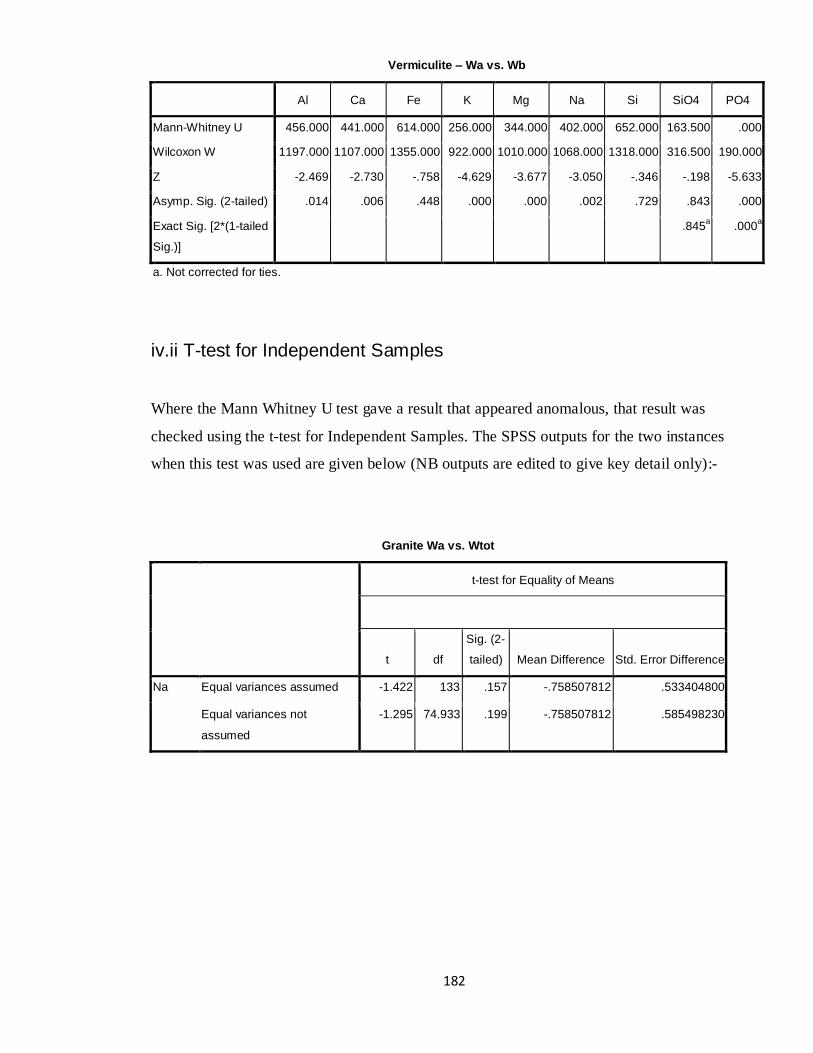
182
Vermiculite – Wa vs. Wb
Al Ca Fe K Mg Na Si SiO4 PO4
Mann-Whitney U 456.000 441.000 614.000 256.000 344.000 402.000 652.000 163.500 .000
Wilcoxon W 1197.000 1107.000 1355.000 922.000 1010.000 1068.000 1318.000 316.500 190.000
Z -2.469 -2.730 -.758 -4.629 -3.677 -3.050 -.346 -.198 -5.633
Asymp. Sig. (2-tailed) .014 .006 .448 .000 .000 .002 .729 .843 .000
Exact Sig. [2*(1-tailed
Sig.)]
.845a .000
a
a. Not corrected for ties.
iv.ii T-test for Independent Samples
Where the Mann Whitney U test gave a result that appeared anomalous, that result was
checked using the t-test for Independent Samples. The SPSS outputs for the two instances
when this test was used are given below (NB outputs are edited to give key detail only):-
Granite Wa vs. Wtot
t-test for Equality of Means
t df
Sig. (2-
tailed) Mean Difference Std. Error Difference
Na Equal variances assumed -1.422 133 .157 -.758507812 .533404800
Equal variances not
assumed
-1.295 74.933 .199 -.758507812 .585498230

183
Granite Wa vs. Wb
t-test for Equality of Means
t df
Sig. (2-
tailed) Mean Difference Std. Error Difference
SiO4 Equal variances assumed -2.077 62 .042 -.135357 .065174
Equal variances not
assumed
-2.037 43.008 .048 -.135357 .066455
PO4 Equal variances assumed -2.807 62 .007 -.058035 .020675
Equal variances not
assumed
-2.738 36.885 .009 -.058035 .021194
Vermiculite Wa vs. Wb
t-test for Equality of Means
t df
Sig. (2-
tailed) Mean Difference Std. Error Difference
SiO4 Equal variances assumed -.360 35 .721 -.016765 .046618
Equal variances not
assumed
-.357 32.639 .724 -.016765 .047018
PO4 Equal variances assumed -7.405 36 .000 -.531579 .071783
Equal variances not
assumed
-7.405 18.000 .000 -.531579 .071783
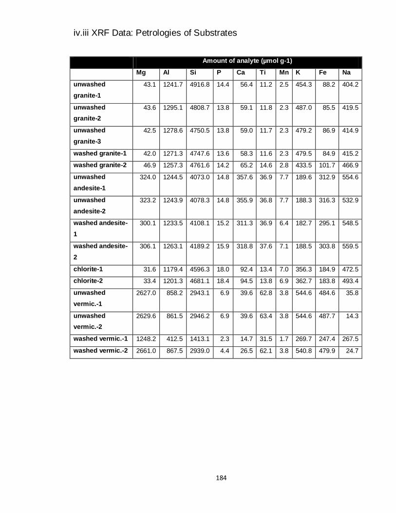
184
iv.iii XRF Data: Petrologies of Substrates
Amount of analyte (µmol g-1)
Mg Al Si P Ca Ti Mn K Fe Na
unwashed
granite-1
43.1 1241.7 4916.8 14.4 56.4 11.2 2.5 454.3 88.2 404.2
unwashed
granite-2
43.6 1295.1 4808.7 13.8 59.1 11.8 2.3 487.0 85.5 419.5
unwashed
granite-3
42.5 1278.6 4750.5 13.8 59.0 11.7 2.3 479.2 86.9 414.9
washed granite-1 42.0 1271.3 4747.6 13.6 58.3 11.6 2.3 479.5 84.9 415.2
washed granite-2 46.9 1257.3 4761.6 14.2 65.2 14.6 2.8 433.5 101.7 466.9
unwashed
andesite-1
324.0 1244.5 4073.0 14.8 357.6 36.9 7.7 189.6 312.9 554.6
unwashed
andesite-2
323.2 1243.9 4078.3 14.8 355.9 36.8 7.7 188.3 316.3 532.9
washed andesite-
1
300.1 1233.5 4108.1 15.2 311.3 36.9 6.4 182.7 295.1 548.5
washed andesite-
2
306.1 1263.1 4189.2 15.9 318.8 37.6 7.1 188.5 303.8 559.5
chlorite-1 31.6 1179.4 4596.3 18.0 92.4 13.4 7.0 356.3 184.9 472.5
chlorite-2 33.4 1201.3 4681.1 18.4 94.5 13.8 6.9 362.7 183.8 493.4
unwashed
vermic.-1
2627.0 858.2 2943.1 6.9 39.6 62.8 3.8 544.6 484.6 35.8
unwashed
vermic.-2
2629.6 861.5 2946.2 6.9 39.6 63.4 3.8 544.6 487.7 14.3
washed vermic.-1 1248.2 412.5 1413.1 2.3 14.7 31.5 1.7 269.7 247.4 267.5
washed vermic.-2 2661.0 867.5 2939.0 4.4 26.5 62.1 3.8 540.8 479.9 24.7

185
iv.iv Data Summaries
Summaries are presented of the key experimental data below. See §1.9 p33 for a description of
the data labels.
iv.iv.i Granite Aggregated Data
Below are summaries of the granite aggregated dataset formed using population means ( )
formed from the 30/4/08, 24/6/08, 2/9/08, 19/12/08, 12/1/09 and 30/7/09 experiments:-
Al Ca Fe K Mg Na Si SiO(4) PO(4)
Wa 0.01159 1.66429 0.00211 0.66892 0.42707 2.90788 0.34608 0.26100 0.01365
Wa st error 0.02558 0.17155 0.00166 0.03051 0.04653 0.44054 0.07232 0.01810 0.01104
Wb 0.01324 1.25229 0.00489 0.65776 0.34416 3.12012 0.43524 0.43042 0.05893
Wb st error 0.00548 0.37423 0.00258 0.09635 0.12435 0.34917 0.11106 0.07646 0.02841
Wmoss 0.17733 1.16711 0.23239 1.08393 0.31168 0.68583 0.11883
Wmoss st error 0.01182 0.07823 0.01516 0.07211 0.01123 0.06719 0.00814
Wtot 0.19063 2.42063 0.23728 1.73905 0.65674 3.78800 0.55057
Wtot st error 0.00964 0.32049 0.01510 0.09119 0.11185 0.35467 0.11454
Wnetbio 0.17904 0.75634 0.23517 1.07013 0.22967 0.88012 0.20449
Data normalised to Wa
Al Ca Fe K Mg Na Si SiO(4) PO(4)
Wa 1 1 1 1 1 1 1 1 1
Wa st error 2.20745 0.10308 0.78953 0.04562 0.10895 0.15150 0.20896 0.06934 0.80846
Wb 1.14220 0.75244 2.31761 0.98331 0.80587 1.07299 1.25762 1.64912 4.31648
Wb st error 0.47269 0.22486 1.22557 0.14404 0.29118 0.12008 0.32092 0.29296 2.08114
Wmoss 15.30153 0.70126 110.23765 1.62040 0.72982 0.23585 0.34335
Wmoss st error 1.02007 0.04701 7.19317 0.10779 0.02629 0.02311 0.02352 Wtot (Ψ) 16.44904 1.45445 112.55797 2.59978 1.53779 1.30267 1.59085
Wtot st error 0.83150 0.19257 7.16401 0.13632 0.26191 0.12197 0.33095
Wnetbio 15.44904 0.45445 111.55797 1.59978 0.53779 0.30267 0.59085

186
iv.iv.ii Andesite Aggregated Data
Below are summaries of the andesite aggregated dataset formed using population means ( ) of
the data from the 28/11/08, 2/12/08 and 25/1/09 experiments:-
Al Ca Fe K Mg Na Si
Wa 0.00631 1.35620 0.00066 0.56301 0.11933 5.29233 0.14772
Wa st error 0.00092 0.22096 0.00000 0.03722 0.02860 0.51847 0.00656
Wb 0.00554 1.79834 0.00088 0.72011 0.14360 4.49034 0.13725
Wb st error 0.00029 0.15417 0.00021 0.02856 0.01251 0.37599 0.00100
Wmoss 0.24763 3.92502 0.21555 0.29864 0.53853 0.32773 0.11994
Wmoss st
error 0.10443 1.96780 0.09314 0.13172 0.18872 0.41129 0.03691
Wtot 0.25509 5.59055 0.21843 1.01875 0.68404 4.81260 0.25674
Wtot st error 0.08678 1.78801 0.08081 0.14836 0.16549 0.28316 0.03317
Wnetbio 0.24353 4.23711 0.21306 0.45800 0.55234 -0.52964 0.10537
Data normalised to Wa
Al Ca Fe K Mg Na Si
Wa 1 1 1 1 1 1 1
Wa st error 0.14631 0.16292 0.00000 0.06611 0.23971 0.09797 0.04441
Wb 0.87753 1.32601 1.33505 1.27904 1.20341 0.84846 0.92915
Wb st error 0.04524 0.11368 0.32082 0.05073 0.10482 0.07104 0.00676
Wmoss 39.22408 2.89413 326.28832 0.53043 4.51298 0.06192 0.81198
Wmoss st
error 16.54217 1.45097 140.98552 0.23396 1.58149 0.07771 0.24984
Wtot (Ψ) 40.40679 4.12221 330.65068 1.80947 5.73244 0.90936 1.73802
Wtot st error 13.74579 1.31839 122.32354 0.26351 1.38685 0.05350 0.22454
Wnetbio 38.57553 3.12425 322.51473 0.81349 4.62875 -0.10008 0.71333

187
iv.iv.iii Vermiculite Aggregated Data
Below are summaries of the vermiculite aggregated dataset formed using population means
( ) formed from the 14/2/08 and 17/2/09 experiments:-
Al Ca Fe K Mg Na Si
Wa 0.01091 0.07510 0.01068 1.29317 0.23883 2.85130 0.60873
Wa 95% conf. 0.00778 0.10409 0.00295 0.19934 0.04594 0.52320 0.05529
Wb 0.00524 0.09247 0.00902 2.05233 0.51200 3.58357 0.66645
Wb 95% conf. 0.00265 0.04140 0.00274 0.24759 0.12552 0.48026 0.08609
Wmoss 0.38175 0.18637 0.30044 0.37382 1.70899 1.96408 0.34345
Wmoss 95%
conf. 0.09013 0.02765 0.07255 0.06899 0.39645 0.61704 0.09419
Wtot 0.38699 0.27883 0.30946 2.42616 2.22100 5.54766 1.00989
Wtot 95% conf. 0.09006 0.04534 0.07254 0.26067 0.38120 0.69968 0.15063
Wnetbio 0.37608 0.20374 0.29878 1.13299 1.98217 2.69636 0.40116
Data normalised to Wa
Al Ca Fe K Mg Na Si
Wa 1 1 1 1 1 1 1
Wa 95% conf. 0.71304 1.38611 0.27624 0.15415 0.19237 0.18350 0.09083
Wb 0.48076 1.23129 0.84473 1.58706 2.14381 1.25682 1.09481
Wb 95% conf. 0.24288 0.55133 0.25652 0.19146 0.52555 0.16844 0.14142
Wmoss 35.00437 2.48168 28.13145 0.28908 7.15572 0.68884 0.56420
Wmoss 95%
conf. 8.26490 0.36820 6.79295 0.05335 1.65999 0.21641 0.15472
Wtot (Ψ) 35.48513 3.71297 28.97618 1.87614 9.29953 1.94566 1.65900
Wtot 95% conf. 8.25810 0.60372 6.79250 0.20158 1.59610 0.24539 0.24745
Wnet_bio 34.48513 2.71297 27.97618 0.87614 8.29953 0.94566 0.65900

188
iv.iv.iv 24/6/08 Chlorite Data
Below are summaries of the data from the 24/6/08 chlorite experiment (data are simple
arithmetic means ( x )):-
Al Ca Fe K Mg Na Si SiO(4) PO(4)
Wa 0.02099 1.94595 0.00465 0.55352 0.20858 5.09488 0.13684 0.26905 0.00714
Wa 95% conf. 0.01065 0.31210 0.00214 0.07974 0.01936 2.48086 0.01867 0.02636 0.01748
Wb 0.00890 1.08211 0.00603 0.24067 0.09248 2.34413 0.13333 0.27569 0.00525
Wb 95% conf. 0.00281 0.17138 0.00670 0.03401 0.01128 1.56304 0.01983 0.00812 0.00918
Wmoss 0.08225 3.02756 0.17227 3.36380 0.41794 4.34899 0.01728
Wmoss (95%
conf.) 0.01975 0.24788 0.04281 0.21208 0.07607 0.76200 0.01500
Wtot 0.09115 4.10967 0.17830 3.60447 0.51042 6.69312 0.15061
Wtot 95%
conf. 0.01957 0.24746 0.04335 0.22430 0.07257 1.23076 0.03325
Wnetbio 0.07016 2.16372 0.17365 3.05095 0.30184 1.59824 0.01377
Data normalised to Wa
Al Ca Fe K Mg Na Si SiO(4) PO(4)
Wa 1 1 1 1 1 1 1 1 1
Wa 95% conf. 0.50773 0.16038 0.45991 0.14406 0.09281 0.48693 0.13643 0.09798 2.44691
Wb 0.42403 0.55608 1.29736 0.43480 0.44340 0.46010 0.97432 1.02467 0.73502
Wb 95% conf. 0.13368 0.08807 1.43948 0.06145 0.05408 0.30679 0.14491 0.03019 1.28468
Wmoss 3.91925 1.55583 37.03268 6.07715 2.00371 0.85360 0.12627
Wmoss 95%
conf. 0.94135 0.12738 9.20324 0.38316 0.36470 0.14956 0.10964
Wtot (Ψ) 4.34329 2.11191 38.33004 6.51195 2.44711 1.31369 1.10059
Wtot 95%
conf. 4.34329 2.11191 38.33004 6.51195 2.44711 1.31369 1.10059
Wnetbio 0.93275 0.12716 9.31879 0.40523 0.34793 0.24157 0.24301

189
iv.iv.v 30/7/09 Inoculum Only Experiments
Below are summaries of the data from the 30/7/09 inoculum only experiments (data are simple
arithmetic means ( x )):-
Bare (No Substrate)
Al Ca Fe K Mg Na Si
Wb 0.00957 0.08514 0.00072 0.00741 0.00484 1.80958 0.00251
Wb 95% conf. 0.00815 0.11371 0.00012 0.00000 0.00572 0.40379 0.00000
Wmoss 0.00482 0.26452 0.02141 0.23377 0.08575 0.01798 0.00137
Wmoss 95%
conf. 0.00379 0.00000 0.00521 0.03852 0.00000 0.00370 0.00034
Wtot 0.01440 0.34966 0.02213 0.24118 0.09059 1.82757 0.00389
Wtot 95% conf. 0.00860 0.11371 0.00519 0.03852 0.00572 0.40441 0.00034
With Substrate (Granite)
Al Ca Fe K Mg Na Si
Wa 0.00568 2.20679 0.00071 0.69585 0.54881 4.03563 0.28184
Wa 95% conf. 0.00651 0.31431 0.00010 0.11024 0.08548 1.10540 0.03522
Wb 0.01119 1.26556 0.00081 0.37520 0.25393 2.65129 0.31591
Wb 95% conf. 0.01862 0.53473 0.00033 0.14191 0.05867 0.64059 0.04336
Wmoss 0.14157 0.55193 0.15029 0.80065 0.18005 0.03553 0.11877
Wtot 0.15276 1.81749 0.15110 1.17585 0.43398 2.68682 0.43467
Wtot 95% conf. 0.03467 0.61370 0.02870 0.19633 0.08888 0.65455 0.04757
Wnetbio 0.14708 -
0.38930 0.15039 0.48000 -
0.11482 -
1.34881 0.15284

190
Summary
Al Ca Fe K Mg Na Si
Bare total 0.01440 0.34966 0.02213 0.24118 0.09059 1.82757 0.00389
Granite total 0.15276 1.81749 0.15110 1.17585 0.43398 2.68682 0.43467
Bare 95% conf. 0.00860 0.11371 0.00519 0.03852 0.00572 0.40441 0.00034
Granite 95%
conf. 0.03467 0.61370 0.02870 0.19633 0.08888 0.65455 0.04757
Summary normalised to Wa
Al Ca Fe K Mg Na Si
Bare total 1 1 1 1 1 1 1
Granite total 10.61182 5.19790 6.82848 4.87541 4.79068 1.47016 111.84931
Bare 95% conf. 0.59711 0.32519 0.23451 0.15972 0.06319 0.22128 0.08795
Granite 95%
conf. 2.40863 1.75513 1.29691 0.81405 0.98118 0.35815 12.24084

191
iv.v Amounts of NAA analytes in Aqueous Microcosm Components
Below is a table showing the amounts of silicate (SiO44-
) and phosphate (PO43-
) in the aqueous
microcosm components (corrected for filtrate blanks) analysed using the NAA. No correction
was needed for upH2O as there was no measurable SiO44-
or PO43-
contamination in upH2O.
NB a blank cell means that there is no successful analysis for that analyte due to an
instrumental problem. Amount of
analyte
Tube Cosm. (µmol)
Round No Date No Subs. Treat. SiO(4) PO(4)
3 77 14/02/2008 11 Vermic. Control 0.09 0.00
3 78 14/02/2008 12 Vermic. Control 0.16 0.00
3 79 14/02/2008 13 Vermic. Control 0.25 0.00
3 80 14/02/2008 14 Vermic. Control 0.37 0.00
3 81 14/02/2008 15 Vermic. Control 0.43 0.00
3 82 14/02/2008 16 Vermic. Control 0.24 0.00
3 83 14/02/2008 17 Vermic. Control 0.00
3 84 14/02/2008 18 Vermic. Control 0.38 0.00
3 85 14/02/2008 19 Vermic. Control 0.00
3 86 14/02/2008 20 Vermic. Control 0.00
3 97 14/02/2008 31 Vermic. Control 0.48 0.00
3 98 14/02/2008 32 Vermic. Control 0.49 0.00
3 99 14/02/2008 33 Vermic. Control 0.49 0.00
3 100 14/02/2008 34 Vermic. Control 0.53 0.00
3 101 14/02/2008 35 Vermic. Control 0.52 0.00
3 102 14/02/2008 36 Vermic. Control 0.59 0.00
3 103 14/02/2008 37 Vermic. Control 0.55 0.00
3 104 14/02/2008 38 Vermic. Control 0.57 0.00
3 105 14/02/2008 39 Vermic. Control 0.46 0.00
3 106 14/02/2008 40 Vermic. Control 0.51
3 67 14/02/2008 1 Vermic. Mossed 0.65 0.97
3 68 14/02/2008 2 Vermic. Mossed 0.22
3 69 14/02/2008 3 Vermic. Mossed 0.50 0.71
3 70 14/02/2008 4 Vermic. Mossed 0.37 0.07
3 71 14/02/2008 5 Vermic. Mossed 0.16 0.58
3 72 14/02/2008 6 Vermic. Mossed 0.60 0.33
3 73 14/02/2008 7 Vermic. Mossed 0.32 0.08
3 74 14/02/2008 8 Vermic. Mossed 0.51 0.89
3 75 14/02/2008 9 Vermic. Mossed 0.42 0.89
3 76 14/02/2008 10 Vermic. Mossed 0.28 0.07
3 87 14/02/2008 21 Vermic. Mossed 0.56 0.53
3 88 14/02/2008 22 Vermic. Mossed 0.57 0.54
3 89 14/02/2008 23 Vermic. Mossed 0.59 0.22
3 90 14/02/2008 24 Vermic. Mossed 0.56 0.37
3 91 14/02/2008 25 Vermic. Mossed 0.43 0.87
3 92 14/02/2008 26 Vermic. Mossed 0.39 0.60
3 93 14/02/2008 27 Vermic. Mossed 0.39 0.73
3 94 14/02/2008 28 Vermic. Mossed 0.30 0.61
3 95 14/02/2008 29 Vermic. Mossed 0.42 0.92

192
Amount of
analyte
Tube Cosm. (µmol)
Round No Date No Subs. Treat. SiO(4) PO(4)
3 96 14/02/2008 30 Vermic. Mossed 0.46 0.12
4 23 30/04/2008 1 Granite Control 0.28 0.00
4 24 30/04/2008 4 Granite Control 0.28 0.05
4 25 30/04/2008 7 Granite Control 0.08 0.04
4 26 30/04/2008 8 Granite Control 0.71 0.11
4 27 30/04/2008 10 Granite Control 0.29 0.00
4 28 30/04/2008 11 Granite Control 0.29 0.00
4 29 30/04/2008 13 Granite Control 0.28 0.00
4 30 30/04/2008 14 Granite Control 0.28 0.00
4 31 30/04/2008 17 Granite Control 0.28 0.00
4 32 30/04/2008 19 Granite Control 0.28 0.00
4 43 30/04/2008 2 Granite Mossed 0.28 0.05
4 44 30/04/2008 3 Granite Mossed 0.00 0.00
4 45 30/04/2008 5 Granite Mossed 0.00 0.00
4 46 30/04/2008 6 Granite Mossed 0.94 0.17
4 47 30/04/2008 9 Granite Mossed 0.89 0.12
4 48 30/04/2008 12 Granite Mossed 1.16 0.10
4 49 30/04/2008 15 Granite Mossed 0.79 0.01
4 50 30/04/2008 16 Granite Mossed 0.68 0.16
4 51 30/04/2008 18 Granite Mossed 0.72 0.00
4 52 30/04/2008 20 Granite Mossed 0.77 0.00
4 57 24/06/2008 13 Chlorite Control 0.20 0.00
4 58 24/06/2008 14 Chlorite Control 0.28 0.00
4 59 24/06/2008 15 Chlorite Control 0.28 0.05
4 65 24/06/2008 21 Chlorite Control 0.28 0.00
4 67 24/06/2008 23 Chlorite Control 0.28 0.00
4 68 24/06/2008 24 Chlorite Control 0.28 0.00
4 69 24/06/2008 25 Chlorite Control 0.28 0.00
4 60 24/06/2008 16 Chlorite Mossed 0.28 0.00
4 61 24/06/2008 17 Chlorite Mossed 0.28 0.00
4 62 24/06/2008 18 Chlorite Mossed 0.28 0.00
4 63 24/06/2008 19 Chlorite Mossed 0.26 0.00
4 64 24/06/2008 20 Chlorite Mossed 0.28 0.00
4 66 24/06/2008 22 Chlorite Mossed 0.28 0.01
4 70 24/06/2008 26 Chlorite Mossed 0.28 0.03
4 72 24/06/2008 28 Granite Control 0.28 0.00
4 75 24/06/2008 31 Granite Control 0.12 0.00
4 76 24/06/2008 32 Granite Control 0.17 0.00
4 77 24/06/2008 33 Granite Control 0.00 0.00
5 21 24/06/2008 35 Granite Control 0.31 0.00
5 23 24/06/2008 37 Granite Control 0.34 0.00
5 29 24/06/2008 44 Granite Control 0.67 0.00
5 30 24/06/2008 47 Granite Control 0.58 0.00
5 32 24/06/2008 49 Granite Control 0.24 0.00
5 33 24/06/2008 50 Granite Control 0.32 0.00
4 71 24/06/2008 27 Granite Mossed 0.28 0.00
4 73 24/06/2008 29 Granite Mossed 0.00 0.00

193
Amount of
analyte
Tube Cosm. (µmol)
Round No Date No Subs. Treat. SiO(4) PO(4)
4 74 24/06/2008 30 Granite Mossed 0.20 0.00
4 78 24/06/2008 34 Granite Mossed 0.14 0.00
5 22 24/06/2008 36 Granite Mossed 0.34 0.00
5 24 24/06/2008 38 Granite Mossed 0.35 0.00
5 25 24/06/2008 39 Granite Mossed 1.08 0.00
5 26 24/06/2008 40 Granite Mossed 0.57 0.00
5 27 24/06/2008 42 Granite Mossed 0.81 0.00
5 28 24/06/2008 43 Granite Mossed 0.87 0.00
5 31 24/06/2008 48 Granite Mossed 0.91 0.00
6 18 15/08/2008 2 Chlorite Control 0.05 0.00
6 20 15/08/2008 4 Chlorite Control 0.04 0.00
6 22 15/08/2008 6 Chlorite Control 0.05 0.00
6 24 15/08/2008 8 Chlorite Control 0.05 0.00
6 17 15/08/2008 1 Chlorite Mossed 0.04 0.00
6 19 15/08/2008 3 Chlorite Mossed 0.04 0.01
6 21 15/08/2008 5 Chlorite Mossed 0.06 0.00
6 23 15/08/2008 7 Chlorite Mossed 0.05 0.01
6 26 15/08/2008 10 Granite Control 0.08 0.00
6 28 15/08/2008 12 Granite Control 0.04 0.00
6 25 15/08/2008 9 Granite Mossed 0.12 0.07
6 27 15/08/2008 11 Granite Mossed 0.12 0.07
6 30 02/09/2008 2 Granite Control 0.08 0.00
6 32 02/09/2008 4 Granite Control 0.22 0.00
6 33 02/09/2008 5 Granite Control 0.22 0.00
6 34 02/09/2008 6 Granite Control 0.24 0.00
6 35 02/09/2008 7 Granite Control 0.09 0.00
6 38 02/09/2008 10 Granite Control 0.20
6 71 02/09/2008 13 Granite Control 0.05 0.00
6 72 02/09/2008 14 Granite Control 0.19 0.00
6 77 02/09/2008 19 Granite Control 0.02 0.00
6 78 02/09/2008 20 Granite Control 0.11 0.00
6 80 02/09/2008 22 Granite Control 0.45 0.16
6 85 02/09/2008 27 Granite Control 0.18 0.12
6 88 02/09/2008 30 Granite Control 0.22 0.00
6 29 02/09/2008 1 Granite Mossed 0.27 0.00
6 31 02/09/2008 3 Granite Mossed 0.28 0.03
6 36 02/09/2008 8 Granite Mossed 0.21 0.19
6 37 02/09/2008 9 Granite Mossed 0.16 0.10
6 73 02/09/2008 15 Granite Mossed 0.24 0.52
6 74 02/09/2008 16 Granite Mossed 0.35 0.21
6 75 02/09/2008 17 Granite Mossed 0.27 0.25
6 76 02/09/2008 18 Granite Mossed 0.13 0.01
6 79 02/09/2008 21 Granite Mossed 0.17 0.00
6 81 02/09/2008 23 Granite Mossed 0.09 0.00
6 82 02/09/2008 24 Granite Mossed 0.39 0.04
6 83 02/09/2008 25 Granite Mossed 0.10 0.08
6 84 02/09/2008 26 Granite Mossed 0.28 0.00

194
Amount of
analyte
Tube Cosm. (µmol)
Round No Date No Subs. Treat. SiO(4) PO(4)
6 86 02/09/2008 28 Granite Mossed 0.20 0.11
6 87 02/09/2008 29 Granite Mossed 0.21 0.11