quantifying uncertainty and sampling quality in

CHAPTER 2Quantifying Uncertainty andSampling Quality in BiomolecularSimulations

Alan Grossfield1 and Daniel M. Zuckerman2

Contents 1. Introduction 241.1 Examples big and small: butane and rhodopsin 251.2 Absolute vs. relative convergence 271.3 Known unknowns 291.4 Non-traditional simulation methods 30

2. Error Estimation in Single Observables 312.1 Correlation-time analysis 312.2 Block averaging 332.3 Summary — single observables in dynamical simulations 352.4 Analyzing single observables in non-dynamical simulations 36

3. Overall Sampling Quality in Simulations 373.1 Qualitative and visual analyses of overall sampling

effectiveness 373.2 Quantifying overall sampling quality: the effective sample size 413.3 Analyzing non-standard simulations — for example, replica

exchange 434. Recommendations 44Acknowledgments 45References 45Appendix 47

1Department of Biochemistry and Biophysics, University of Rochester Medical Center, Rochester, NY, USA2Department of Computational Biology, University of Pittsburgh School of Medicine, Pittsburgh, PA, USA

Annual Reports in Computational Chemistry, Volume 5 r 2009 Elsevier B.V.ISSN: 1574-1400, DOI 10.1016/S1574-1400(09)00502-7 All rights reserved.

23

Abstract Growing computing capacity and algorithmic advances have facilitated thestudy of increasingly large biomolecular systems at longer timescales.However, with these larger, more complex systems come questions aboutthe quality of sampling and statistical convergence. What size systems canbe sampled fully? If a system is not fully sampled, can certain ‘‘fast variables’’be considered well converged? How can one determine the statisticalsignificance of observed results? The present review describes statisticaltools and the underlying physical ideas necessary to address thesequestions. Basic definitions and ready-to-use analyses are provided, alongwith explicit recommendations. Such statistical analyses are of paramountimportance in establishing the reliability of simulation data in any givenstudy.

Keywords: error analysis; principal component; block averaging;convergence; sampling quality; equilibrium ensemble; correlation time;ergodicity

1. INTRODUCTION

It is a well-accepted truism that the results of a simulation are only as good as thestatistical quality of the sampling. To compensate for the well-known samplinglimitations of conventional molecular dynamics (MD) simulations of evenmoderate-size biomolecules, the field is now witnessing the rapid proliferation ofmultiprocessor computing, new algorithms, and simplified models. Thesechanges underscore the pressing need for unambiguous measures of samplingquality. Are current MD simulations long enough to make quantitativepredictions? How much better are the new algorithms than the old? Can evensimplified models be fully sampled?

Overall, errors in molecular simulation arise from two factors: inaccuracy inthe models and insufficient sampling. The former is related to choices inrepresenting the system, for example, all-atom vs. coarse grained models, fixedcharge vs. polarizable force fields, and implicit vs. explicit solvent, as well astechnical details like the system size, thermodynamic ensemble, and integrationalgorithm used. Taken in total, these choices define the model used to representthe system of interest. The second issue, quality of sampling, is largelyorthogonal to the choice of model. In some sense, assessing the quality of thesampling is a way of asking how accurately a given quantity was computed forthe chosen model. While this review will focus on the issue of sampling, it isimportant to point out that without adequate sampling, the predictions of theforce fields remain unknown: very few conclusions, positive or negative, can bedrawn from an undersampled calculation. Those predictions are embodied mostdirectly in the equilibrium ensemble that simulations have apparently failed toproduce in all but small-molecule systems [1,2]. Thus, advances in force fielddesign and parameterization for large biomolecules must proceed in parallelwith sampling advances and their assured quantification.

24 Alan Grossfield and Daniel M. Zuckerman

This review will attempt to acquaint the reader with the most important ideasin assessing sampling quality. We will address both the statistical uncertainty inindividual observables and quantification of the global quality of the equilibriumensemble. We will explicitly address differing approaches necessary for standarddynamics simulations, as compared to algorithms such as replica exchange, andwhile we use the language of MD, virtually all of the arguments apply equally toMonte Carlo (MC) methods as well. Although this review will not specificallyaddress path sampling, many of the ideas carry over to what amounts toequilibrium sampling of the much larger space of paths. We will recommendspecific ‘‘best practices,’’ with the inevitable bias toward the authors’ work. Wehave tried to describe the intellectual history behind the key ideas, but the articleis ultimately organized around practically important concepts.

For the convenience of less experienced readers, key terms and functions havebeen defined in the appendix: average, variance, correlation function, andcorrelation time.

1.1 Examples big and small: butane and rhodopsin

Example trajectories from small and large systems (to which we will returnthroughout the review) illustrate the key ideas. In fact, almost all the complexitywe will see in large systems is already present in a molecule as simple as n-butane. Nevertheless, it is very valuable to look at both ‘‘very long’’ trajectoriesand some that are ‘‘not long enough.’’ Concerning the definition of ‘‘long,’’ wehope that if ‘‘we know it when we see it,’’ then we can construct a suitablemathematical definition. Visual confirmation of good sampling is still animportant check on any quantitative measure.

1.1.1 ButaneLet us first consider butane, as in Figure 1. Several standard molecularcoordinates are plotted for a period of 1 ns, and it is clear that several timescalesless than 1 ns are present. The very fastest motions (almost vertical in the scale ofthe figure) correspond to bond length and angle vibrations, while the dihedralsexhibit occasional quasi-discrete transitions. The CH3 dihedral, which reports onmethyl spinning, clearly makes more frequent transitions than the main dihedral.

Perhaps the trajectory of butane’s C–C–C angle is most ambiguous, sincethere appears to be a slow overall undulation in addition to the rapid vibrations.The undulation appears to have a frequency quite similar to the transition rate ofthe main dihedral, and underscores the point that generally speaking, all degrees offreedom are coupled, as sketched in Figure 2. In the case of butane, the samplingquality of the C–C–C angle may indeed be governed by the slowest motions ofthe molecule and isomerization of the central torsion.

1.1.2 RhodopsinIt is perhaps not surprising that all of the degrees of freedom are tightly coupled ina simple system like butane. It seems reasonable that this coupling may be lessimportant in larger biomolecular systems, where there are motions on timescales

Quantifying Uncertainty and Sampling Quality in Biomolecular Simulations 25

-100

-50

0

50

100

150

200

0 200 400 600 800 1000

C-C

-C-H

Dih

edra

l Ang

le

Time (psec)

100

105

110

115

120

125

0 200 400 600 800 1000

C-C

-C B

ond

Ang

le

Time (psec)

0

50

100

150

200

250

300

350

0 200 400 600 800 1000

C-C

-C-C

Dih

edra

l Ang

le

Time (psec)

Figure 1 Widely varying timescales in n-butane. Even the simple butane molecule (upper left)exhibits a wide variety of dynamical timescales, as exhibited in the three time traces. Even inthe fast motions of the C–C–C bond angle, a slow undulation can be detected visually.

-1

-0.5

0

0.5

1

-1.5 -1 -0.5 0 0.5 1 1.5

Y

X

B

A

Figure 2 Slow and fast timescales are generally coupled. The plot shows a schematictwo-state potential. The y coordinate is fast regardless of whether state A or B is occupied.However, fast oscillations of y are no guarantee of convergence because the motions in x willbe much slower. In a molecule, all atoms interact — even if weakly or indirectly — and suchcoupling must be expected.


ranging from femtoseconds to milliseconds; indeed, it is commonly assumed thatsmall-scale reorganizations, such as side-chain torsions in proteins, can becomputed with confidence from MD simulations of moderate length. While thisassumption is likely true in many cases, divining the cases when it holds canbe extremely difficult. As a concrete example, consider the conformation of theretinal ligand in dark-state rhodopsin. The ligand is covalently bound inside theprotein via Schiff base linkage to an internal lysine, and contains an aromatichydrocarbon chain terminated by an ionone ring. This ring packs against a highlyconserved tryptophan residue, and is critical to this ligand’s role as an inverseagonist.

The ring’s orientation, relative to the hydrocarbon chain, is largely describedby a single torsion, and one might expect that this kind of local quantity would berelatively easy to sample in a MD simulation. The quality of sampling for thistorsion would also seem easy to assess, because as for most torsions, there arethree stable states. However, Figure 3 shows that this is not the case, because ofcoupling between fast and slow modes. The upper frame of Figure 3 shows atime series of this torsion from a MD simulation of dark-state rhodopsin [3]; thethree expected torsional states (g+, g!, and t) are all populated, and there are anumber of transitions, so most practitioners would have no hesitation inconcluding that (a) the trajectory is reasonably well sampled, and (b) that all threestates are frequently populated, with g! the most likely and trans the least. Themiddle panel, however, shows the same trajectory extended to 150 ns; it tooseems to suggest a clear conclusion, in this case that the transitions in the first50 ns are part of a slow equilibration, but that once the protein has relaxed theretinal is stable in the g! state. The bottom panel, containing the results ofextending the trajectory to 1,600 ns, suggests yet another distinct conclusion, thatg! and t are the predominant states, and rapidly exchange with each other, onthe nanosecond scale.

These results highlight the difficulties involved in assessing the convergenceof single observables. No amount of visual examination of the upper and middlepanels would have revealed the insufficiency of the sampling (although it isinteresting to note that the ‘‘effective sample size’’ described below is not toolarge). Rather, it is only after the fact, in light of the full 1,600 ns trajectory, thatthe sampling flaws in the shorter trajectories become obvious. This highlightsthe importance of considering timescales broadly when designing and inter-preting simulations. This retinal torsion is a local degree of freedom, and assuch should relax relatively quickly, but the populations of its states are coupledto the conformation of the protein as a whole. As a result, converging thesampling for the retinal requires reasonable sampling of the protein’s internaldegrees of freedom, and is thus a far more difficult task than it would firstappear.

1.2 Absolute vs. relative convergence

Is it possible to describe a simulation as absolutely converged? From a statisticalpoint of view, we believe the answer is clearly ‘‘no,’’ except in those cases where


the correct answer is already known by other means. Whether a simulationemploys ordinary MD or a much more sophisticated algorithm, so long as thealgorithm correctly yields canonical sampling according to the Boltzmann factor,one can expect the statistical quality will increase with the duration of thesimulation. In general, the statistical uncertainty of most conceivable molecularsimulation algorithms will decay inversely with the square root of simulationlength. The square-root law should apply once a stochastic simulation process is

-150

-100

-50

0

50

100

150

0 10 20 30 40 50

Tors

ion

angl

e (d

eg)

Time (ns)

-150

-100

-50

0

50

100

150

0 20 40 60 80 100 120 140

Tors

ion

angl

e (d

eg)

Time (ns)

-150

-100

-50

0

50

100

150

0 200 400 600 800 1000 1200 1400 1600

Tors

ion

angl

e (d

eg)

Time (ns)

Figure 3 Time series for the torsion connecting the ionone ring to the chain of rhodopsin’sretinal ligand. All three panels show the same trajectory, cut at 50, 150, and 1,600 ns,respectively.


in the true sampling regime — that is, once it is long enough to produce multipleproperly distributed statistically independent configurations.

The fundamental perspective of this review is that simulation results are notabsolute, but rather are intrinsically accompanied by statistical uncertainty [4–8].Although this view is not novel, it is at odds with informal statements that asimulation is ‘‘converged.’’ Beyond quantification of uncertainty for specificobservables, we also advocate quantification of overall sampling quality in termsof the ‘‘effective sample size’’ [8] of an equilibrium ensemble [9,10].

As a conceptual rule-of-thumb, any estimate for the average of an observablewhich is found to be based on fewer than B20 statistically independentconfigurations (or trajectory segments) should be considered unreliable. Thereare two related reasons for this. First, any estimate of the uncertainty in theaverage based on a small number of observations will be unreliable because thisuncertainty is based on the variance, which converges more slowly than theobservable (i.e., average) itself. Second, any time the estimated number ofstatistically independent observations (i.e., effective sample size) is B20 or less,both the overall sampling quality and the sample-size estimate itself must beconsidered suspect. This is again because sample-size estimation is based onstatistical fluctuations that are, by definition, poorly sampled with so fewindependent observations.

Details and ‘‘best practices’’ regarding these concepts will be given below.

1.3 Known unknowns

1.3.1 Lack of ergodicity — unvisited regions of configuration spaceNo method known to the authors can report on a simulation’s failure to visit animportant region of configuration space unless these regions are already knownin advance. Thus, we instead focus on assessing sampling quality in the regionsof space that has been visited. One can hope that the generation of manyeffectively independent samples in the known regions of configuration spacewith a correct algorithm is good ‘‘insurance’’ against having missed parts of thespace — but certainly it is no guarantee. Larger systems are likely to have morethermodynamically relevant substates, and may thus require more independentsamples even in the absence of significant energetic barriers.

1.3.2 Small states rarely visited in dynamical simulationThis issue is also related to ergodicity, and is best understood through anexample. Consider a potential like that sketched in Figure 4, with two states of98% and 2% population at the temperature of interest. A ‘‘perfect’’ simulationcapable of generating fully independent configurations according to theassociated Boltzmann factor would simply yield 2 of every 100 configurationsin the small state, on average. However, a finite dynamical simulation behavesdifferently. As the barrier between the states gets larger, the frequency of visitingthe small state will decrease exponentially. Thus, estimating an average like /xSwill be very difficult — since the small state might contribute appreciably.Further, quantifying the uncertainty could be extremely difficult if there are only


a small number of visits to the small state — because the variance will be poorlyestimated.

1.4 Non-traditional simulation methods

The preceding discussion applied implicitly to what we classify as dynamicalsimulations — namely, those simulations in which all correlations in the finaltrajectory arise because each configuration is somehow generated from theprevious one. This time-correlated picture applies to a broad class of algorithms:MD, Langevin and Brownian dynamics, as well as traditional Monte Carlo (MC,also known as Markov-chain Monte Carlo). Even though MC may not lead totrue physical dynamics, all the correlations are sequential.

However, in other types of molecular simulation, any sampled configurationmay be correlated with configurations not sequential in the ultimate ‘‘trajectory’’produced. That is, the final result of some simulation algorithms is really a list ofconfigurations, with unknown correlations, and not a true trajectory in the sense of atime series.

One increasingly popular method which lead to non-dynamical trajectories isreplica-exchange MC or MD [11–13], which employs parallel simulations at aladder of temperatures. The ‘‘trajectory’’ at any given temperature includesrepeated visits from a number of (physically continuous) trajectories wanderingin temperature space. Because the continuous trajectories are correlated in theusual sequential way, their intermittent — that is, non-sequential — visits to thevarious specific temperatures produce non-sequential correlations when one ofthose temperatures is considered as a separate ensemble or ‘‘trajectory’’ [14]. Lessprominent examples of non-dynamical simulations occur in a broad class ofpolymer-growth algorithms (e.g., refs. 15–17).

x

U

98%

2%

0

Figure 4 Cartoon of a landscape for which dynamical simulation is intrinsically difficult toanalyze. As the barrier between the states gets higher, the small state requires exponentiallymore dynamical sampling, even though the population may be inconsequential. It would seemthat, in principle, a cutoff should be chosen to eliminate ‘‘unimportant’’ states from analysis.In any complex molecular system, there will always be extremely minor but almostinaccessible basins.


Because of the rather perverse correlations that occur in non-dynamicalmethods, there are special challenges in analyzing statistical uncertainties andsampling quality. This issue has not been well explored in the literature; seehowever [10,18,19]. We therefore present some tentative thoughts on non-dynamical methods, based primarily on the notion that independent simulationsappear to provide the most definitive means for analyzing non-dynamicalsimulations. In the case of replica exchange, understanding the differencebetween ‘‘mixing’’ and sampling will prove critical to any analysis.

2. ERROR ESTIMATION IN SINGLE OBSERVABLES

One of the main goals of biomolecular simulation is the estimation of ensembleaverages, which should always be qualified by estimates of statistical uncertainty.We will review the two main approaches to estimating uncertainty in averages,but a general note of caution should be repeated. Because all variables can becorrelated in a complex system, the so-called ‘‘fast’’ variables may not be as fastas they appear based on standard error estimation techniques: see Figure 2. As inthe examples of the rhodopsin dihedral, above, even a single coordinateundergoing several transitions may not be well sampled. Also, investigatorsshould be wary of judging overall sampling quality based on a small number ofobservables unless they are specifically designed to measure ensemble quality, asdiscussed below.

The present discussion will consider an arbitrary observable f, which is afunction of the configuration x of the system being simulated. The function f(x)could represent a complex measure of an entire macromolecule, such as theradius of gyration, or it could be as simple as a single dihedral or distance.

Our focus will be on time correlations and block averaging. The correlation-time analysis has been in use for some decades [7], including to analyze the firstprotein MD simulation [20], and it embodies the essence of all the single-observable analyses known to the authors. The block-averaging approach [5,21]is explicitly described below because of its relative simplicity and directness inestimating error using simple variance calculations. Block averaging ‘‘short cuts’’the need to calculate a correlation time explicitly, although timescales can beinferred from the results. Similarly, the ‘‘ergodic measure’’ of Thirumalai andcoworkers [22–24], not described here, uses variances and correlation timesimplicitly.

Both the correlation-time analysis and the block-averaging scheme describedbelow assume that a dynamical trajectory is being analyzed. Again, by‘‘dynamical’’ we only mean that correlations are ‘‘transmitted’’ via sequentialconfigurations — which is not true in a method like replica exchange.

2.1 Correlation-time analysis

The correlation-time analysis of a single observable has a very intuitiveunderpinning. Consider first that dynamical simulations (e.g., molecular and


Langevin dynamics), as well as ‘‘quasi-dynamical’’ simulations (e.g., typical MC[25]), create trajectories that are correlated solely based on the sequence of theconfigurations. As described in the Appendix, the correlation time tf measuresthe length of simulation time — whether for physical dynamics or MC —required for the trajectory to lose ‘‘memory’’ of earlier values of f. Therefore, thecorrelation time tf for the specific observable f provides a basis for estimating thenumber of statistically independent values of f present in a simulation of lengthtsim, namely Nind

f " tsim=tf. By itself, Nindf # 1 would suggest good sampling for

the particular observable f.The correlation time is computed from the correlation function (see

Appendix), and it is useful to consider an example. Figure 5 shows the time-correlation functions computed for individual state lifetimes as measured by a100 ns simulation of butane. Specifically, for each snapshot from the trajectory, thecentral torsion was classified as trans, g+, or g!. A time series was then writtenfor each state, with a value of 1 if the system was in that state and 0 otherwise.The autocorrelation functions for each of those time series are shown in Figure 5.All three correlation functions drop smoothly to zero within 200 ps, suggestingthat a 100 ns simulation should contain a very large number of independentsamples. However, the populations for the three states over the course of thetrajectory are 0.78, 0.10, and 0.13 for the trans, g+, and g! states, respectively. Theg+ and g! states are physically identical, and thus should have the samepopulations in the limit of perfect sampling. Thus even a very long simulation ofa very simple system is incapable of estimating populations with high precision.

transg+

g−

1

0.8

0.6

0.4

0.2

0

−0.2

Aut

ocor

rela

tion

0 200 400 600 800 1000

Time (ps)

Figure 5 State autocorrelations computed from 100 ns butane simulations. The centraltorsion was labeled as either trans, g+, or g!, and the autocorrelation function for presence ineach state was computed.


To obtain an estimate of the statistical uncertainty in an average /fS, thecorrelation time tf must be used in conjunction with the variance s2f (square of thestandard deviation; see Appendix) of the observable. By itself, the standarddeviation only gives the basic scale or range of fluctuations in f, which might bemuch larger than the uncertainty of the average /fS. In other words, it is possibleto know very precisely the average of a quantity that fluctuates a lot: as anextreme example, imagine measuring the average height of buildings inManhattan. In a dynamical trajectory, the correlation time tf provides the linkbetween the range of fluctuations and the precision (uncertainty) in an average,which is quantified by the standard error of the mean, SE,

SEðfÞ ¼sfffiffiffiffiffiffiffiffiffiffiNind

f

q " sf

ffiffiffiffiffiffiffiffitftsim

r(1)

In this notation, Nindf is the number of independent samples contained in the

trajectory, and tsim the length of the trajectory. The standard error can be used toapproximate confidence intervals, with a rule of thumb being that 72SErepresents roughly a 95% confidence interval [26]. The actual interval depends onthe underlying distribution and the sampling quality as embodied inNind

f " tsim=tf ; see ref. 25 for a more careful discussion.It has been observed that the simple relation between correlation time and

sampling quality embodied in the estimate Nindf ¼ tsim=tf is actually too

conservative in typical cases [27]. That is, even though the simulation may requirea time tf to ‘‘forget’’ its past (with respect to the observable f ), additionalinformation beyond a single estimate for f is obtained in the period of a singlecorrelation time — that is, from partially correlated configurations. However, theimprovement in sampling quality is modest — the effective sample size may bedouble the estimate based simply on tf. Such subtleties are accounted forautomatically in the block-averaging analysis described below.

Understanding the correlation-time analysis, as well as the habitualcalculation of correlation functions and times, is extremely useful. Yet theanalysis has weaknesses for quantifying uncertainty that suggest relying on otherapproaches for generating publication-quality error bars. First, like any single-observable analysis, the estimation of correlation times may fail to account forslow timescales in observables not considered: recall the rhodopsin example.Second, the calculation of correlation times becomes less reliable in preciselythose situations of greatest interest — when a second, slower timescale enters theintrinsically noisier tail of the correlation function. The third weakness wasalready described: a lack of full accounting for all statistical information in thetrajectory. These latter considerations suggest that a block-averaging procedure,described next, is a preferable analysis of a single observable.

2.2 Block averaging

When executed properly, the block-averaging analysis automatically correctstwo of the weaknesses in correlation-time estimates of the error based on


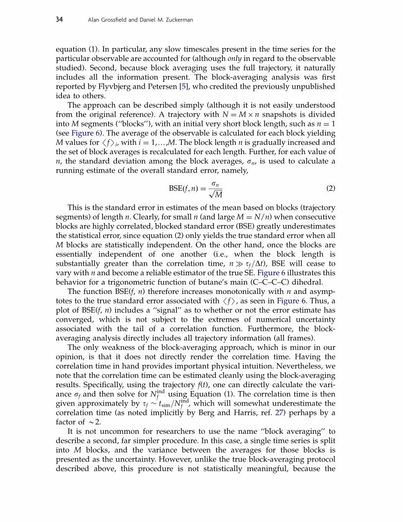
equation (1). In particular, any slow timescales present in the time series for theparticular observable are accounted for (although only in regard to the observablestudied). Second, because block averaging uses the full trajectory, it naturallyincludes all the information present. The block-averaging analysis was firstreported by Flyvbjerg and Petersen [5], who credited the previously unpublishedidea to others.

The approach can be described simply (although it is not easily understoodfrom the original reference). A trajectory with N ¼ M' n snapshots is dividedinto M segments (‘‘blocks’’), with an initial very short block length, such as n ¼ 1(see Figure 6). The average of the observable is calculated for each block yieldingM values for /fSi, with i ¼ 1,y,M. The block length n is gradually increased andthe set of block averages is recalculated for each length. Further, for each value ofn, the standard deviation among the block averages, sn, is used to calculate arunning estimate of the overall standard error, namely,

BSEðf ;nÞ ¼snffiffiffiffiffiM

p (2)

This is the standard error in estimates of the mean based on blocks (trajectorysegments) of length n. Clearly, for small n (and largeM ¼ N/n) when consecutiveblocks are highly correlated, blocked standard error (BSE) greatly underestimatesthe statistical error, since equation (2) only yields the true standard error when allM blocks are statistically independent. On the other hand, once the blocks areessentially independent of one another (i.e., when the block length issubstantially greater than the correlation time, n # tf=Dt), BSE will cease tovary with n and become a reliable estimator of the true SE. Figure 6 illustrates thisbehavior for a trigonometric function of butane’s main (C–C–C–C) dihedral.

The function BSE(f, n) therefore increases monotonically with n and asymp-totes to the true standard error associated with /fS, as seen in Figure 6. Thus, aplot of BSE(f, n) includes a ‘‘signal’’ as to whether or not the error estimate hasconverged, which is not subject to the extremes of numerical uncertaintyassociated with the tail of a correlation function. Furthermore, the block-averaging analysis directly includes all trajectory information (all frames).

The only weakness of the block-averaging approach, which is minor in ouropinion, is that it does not directly render the correlation time. Having thecorrelation time in hand provides important physical intuition. Nevertheless, wenote that the correlation time can be estimated cleanly using the block-averagingresults. Specifically, using the trajectory f(t), one can directly calculate the vari-ance sf and then solve for Nind

f using Equation (1). The correlation time is thengiven approximately by tf " tsim=N

indf , which will somewhat underestimate the

correlation time (as noted implicitly by Berg and Harris, ref. 27) perhaps by afactor of B2.

It is not uncommon for researchers to use the name ‘‘block averaging’’ todescribe a second, far simpler procedure. In this case, a single time series is splitinto M blocks, and the variance between the averages for those blocks ispresented as the uncertainty. However, unlike the true block-averaging protocoldescribed above, this procedure is not statistically meaningful, because the


single-block size is chosen arbitrarily; it is only by systematically varying theblock size that one can reliably draw conclusions about the uncertainty.

2.3 Summary — single observables in dynamical simulations

Several points are worth emphasizing: (i) single observables should not be usedto assess overall sampling quality. (ii) The central ideas in single-observable

0.004

0.006

0.008

0.01

0.012

0.014

0.016

100 200 300 400 500

BS

E =

Blo

cked

Sta

ndar

d E

rror

Block length (psec)

0 0.1 0.2 0.3 0.4 0.5 0.6 0.7 0.8 0.9

1

0 500 1000 1500 2000

cos2 (

C-C

-C-C

)

Time (ps)

Large blocks-weak correlation

Small blocks-strong correlation

Figure 6 The block-averaging procedure considers a full range of block sizes. The upperpanel shows the time series for the squared cosine of the central dihedral of butane, withtwo different block sizes annotated. The lower panel shows the block-averaged standard errorfor that times series, as a function of block size.


analysis are that the correlation time separates statistically independent values ofthe observable, and that one would like to have many statistically independent‘‘measurements’’ of the observable — that is, Nind

f # 1. (iii) The block-averaginganalysis is simple to implement and provides direct estimation of statisticaluncertainty. We recommend that the correlation time and effective sample sizealso be estimated to ensure Nind

f # 1. (iv) In a correlation-time analysis, onewants to ensure the total simulation time is a large multiple of the correlationtime — that is, tsim=tf # 1.

2.4 Analyzing single observables in non-dynamical simulations

As discussed earlier, the essential fact about data from non-dynamicalsimulations (e.g., replica exchange and polymer-growth methods) is that aconfiguration occurring at one point in the ‘‘trajectory’’ may be highly correlatedwith another configuration anywhere else in the final list of configurations.Similarly, a configuration could be fully independent of the immediatelypreceding or subsequent configurations. To put it most simply, the list ofconfigurations produced by such methods is not a time series, and so analysesbased on the explicit or implicit notion of a correlation time (time correlations areimplicit in block averaging) cannot be used.

From this point of view, the only truly valid analysis of statistical errors can beobtained by considering independent simulations. Ideally, such simulationswould be started from different initial conditions to reveal ‘‘trapping’’ (failure toexplore important configurational regions) more readily. Running multiplesimulations appears burdensome, but it is better than excusing ‘‘advanced’’algorithms from appropriate scrutiny. Of course, rather than multiplying theinvestment in computer time, the available computational resources can bedivided into 10 or 20 parts. All these parts, after all, are combined in the finalestimates of observable averages. Running independent trajectories is anexample of an ‘‘embarrassingly parallel’’ procedure, which is often the mostefficient use of a standard computer cluster. Moreover, if a simulation method isnot exploring configuration space well in a tenth of the total run time, then itprobably is not performing good sampling anyway.

How can statistical error be estimated for a single observable fromindependent simulations? There seems little choice but to calculate the standarderror in the mean values estimated from each simulation using Equation (1),where the variance is computed among the averages from the independentsimulations and Nind

f is set to the number of simulations. In essence, eachsimulation is treated as a single measurement, and presumed to be totallyindependent of the other trajectories. Importantly, one can perform a ‘‘realitycheck’’ on such a calculation because the variance of the observable can also becalculated from all data from all simulations — rather than from the simulationmeans. The squared ratio of this absolute variance to the variance of the meansyields a separate (albeit crude) estimate of the number of independent samples.This latter estimate should be of the same order as, or greater than, the number of


independent simulations, indicating that each ‘‘independent’’ simulation indeedcontained at least one statistically independent sample of the observable.

It is interesting to observe that, in replica-exchange simulations, the physicallycontinuous trajectories (which wander in temperature) can be analyzed based ontime-correlation principles [10,14]. Although each samples a non-traditionalensemble, it is statistically well defined and can be used as a proxy for the regularensemble. A more careful analysis could consider, separately, those segments ofeach continuous trajectory at the temperature of interest. The standard erroramong these estimates could be compared to the true variance, as above, toestimate sampling quality. A detailed discussion of these issues in the context ofweighted histogram analysis of replica-exchange simulation is given by Choderaet al. [14].

3. OVERALL SAMPLING QUALITY IN SIMULATIONS

In contrast to measures of convergence that reflect a single local observable, forexample, a torsion angle, some methods focus on the global sampling quality. Fora simulation of a macromolecule, the distinction would be between asking ‘‘howwell do I know this particular quantity?’’ and ‘‘how well have I explored theconformational space of the molecule?’’ The latter question is critical, in that if theconformational space is well sampled, most physical quantities should be knownwell.

This review will describe two classes of analyses of overall sampling quality:(i) qualitative and visual techniques, which are mainly useful in convincingoneself a simulation is not sufficiently sampled; and (ii) quantitative analyses ofsampling, which estimate the ‘‘effective sample size.’’

3.1 Qualitative and visual analyses of overall sampling effectiveness

There are a number of techniques that, although they cannot quantitatively assessconvergence or statistical uncertainty, can give tremendous qualitative insight.While they cannot tell the user that the simulation has run long enough, they canquickly suggest that the simulation has not run long enough. Thus, while theyshould not replace more rigorous methods like block averaging and sample-sizeestimation, they are quite useful.

3.1.1 Scalar RMSD analysesOne of the simplest methods is the comparison of the initial structure of themacromolecule to that throughout the trajectory via a distance measure such asthe root mean square deviation (RMSD). This method is most informative for asystem like a folded protein under native conditions, where the molecule isexpected to spend the vast majority of the time in conformations quite similar tothe crystal structure. If one computes the RMSD time series against the crystalstructure, one expects to see a rapid rise due to thermal fluctuations, followed bya long plateau or fluctuations about a mean at longer timescales. If the RMSD


time series does not reach a steady state, the simulation is either (a) stillequilibrating or (b) drifting away from the starting structure. In any event, untilthe system assumes a steady-state value — one that may fluctuate significantly,but has no significant trend — the system is clearly not converged. Indeed, onecan argue that under that circumstance equilibrium sampling has not yet evenbegun. However, beyond this simple assessment, RMSD is of limited utility,mostly because it contains little information about what states are being sampled;a given RMSD value maps a 3N-dimensional hypersphere of conformation space(for N atoms) to a single scalar, and for all but the smallest RMSD values thishypersphere contains a broad range of structures. Moreover, the limiting valuefor the RMSD cannot be known in advance. We know the value should be non-zero and not large, but the expected plateau value is specific to the systemstudied, and will vary not only between macromolecules, but also with changesto simulation conditions such as temperature and solvent.

An improvement is to use a windowed RMSD function as a measure of therate of conformation change. Specifically, for a given window length (e.g., 10consecutive trajectory snapshots), the average of the all of the pairwise RMSDs(or alternatively, the average deviation from the average over that interval) iscomputed as a function of time. This yields a measure of conformationaldiversity over time, and can more readily reveal conformational transitions.

3.1.2 All-to-all RMSD analysisA more powerful technique is to compute the RMSDs for all pairs of snapshotsfrom the trajectory and plot them on a single graph [28]. Figure 7 shows theresults of such a plot, made using the alpha-carbon RMSD computed from a1.6 ms all-atom simulation of dark-state rhodopsin in an explicit lipid membrane[3]. The plot reveals a hierarchical block structure along the diagonal; thissuggests that the protein typically samples within a substate for a few hundrednanoseconds, and then rapidly transitions to a new conformational well.However, with the exception of two brief excursions occurring around 280 and1,150 ns into the trajectory, the system never appears to leave and then return to agiven substate. This suggests that this simulation, although very long by currentstandards, probably has not fully converged.

3.1.3 Cluster countingA more general approach, also based on pairwise distances, would be to usecluster analysis. Although a general discussion of the many clustering algorithmspresently in use is beyond the scope of this manuscript, for our purposes wedefine clustering to be any algorithm that divides an ensemble into sets of self-similar structures. One application of clustering to the assessment of convergencecame from Daura et al., who measured the rate of discovery of new clusters overthe course of a trajectory; when this rate became very small, the simulation waspresumed to be reasonably well converged [29]. However, a closer look revealsthis criterion to be necessary but not sufficient to guarantee good sampling.While it is true that a simulation that is still exploring new states is unlikely tohave achieved good statistics (at least for a reasonable definition of ‘‘states’’),


simply having visited most of the thermodynamically relevant states is noguarantee that a simulation will produce accurate estimates of observables.

3.1.4 ‘‘Structural histogram’’ of clustersAs discussed by Lyman and Zuckerman [9], not only must clusters be visited, butalso it is important that the populations of those regions be accuratelyreproduced, since the latter provide the weights used to compute thermo-dynamic averages. In a procedure building on this idea, one begins byperforming a cluster analysis on the entire trajectory to generate a vocabularyof clusters or bins. The cluster/bin populations can be arrayed as a one-dimensional ‘‘structural histogram’’ reflecting the full configuration-spacedistribution. Structural histograms from parts of the trajectory are compared toone computed for the full trajectory, and plotting on a log-scale gives thevariation in knot units, indicating the degree of convergence.

3.1.5 Principal components analysisPrincipal component analysis (PCA) is another tool that has been usedextensively to analyze molecular simulations. The technique, which attempts toextract the large-scale characteristic motions from a structural ensemble, was firstapplied to biomolecular simulations by Garcia [28], although an analogoustechnique was used by Levy et al. [30]. The first step is the construction of the3N' 3N (for an N-atom system) fluctuation correlation matrix

Cij ¼ hxi ! x̄iihxj ! x̄ji

where xi represents a specific degree of freedom (e.g., the z-coordinate of the 23rdatom) and the overbar indicates the average structure. This task is commonly

0

0.5

1

1.5

2

2.5

3

0

200

400

600

800

100

0

120

0

140

0

160

0

0

200

400

600

800

1000

1200

1400

1600

Figure 7 All-to-all RMSD for rhodopsin alpha-carbons. The scale bar to the right showsdarker grays to indicate a more similar structures.


simplified by using a subset of the atoms from the molecule of interest (e.g., thea-carbons from the protein backbone). The matrix is then diagonalized toproduce the eigenvalues and eigenvectors; the eigenvectors represent character-istic motions for the system, while each eigenvalue is the mean square fluctuationalong its corresponding vector. The system fluctuations can then be projectedonto the eigenvectors, giving a new time series in this alternative basis set. Thediagonalization and time series projection can be performed efficiently usingsingular value decomposition, first applied to principal component analysis ofbiomolecular fluctuations by Romo et al. [31].

In biomolecular systems characterized by fluctuations around a singlestructure (e.g., equilibrium dynamics of a folded protein), a small number ofmodes frequently account for the vast majority of the motion. As a result, thesystem’s motions can be readily visualized, albeit abstractly, by plotting the timeseries for the projections of the first two or three modes. For example, projectingthe rhodopsin trajectory described above [3] onto its two largest principle modesyields Figure 8. As with the all-to-all RMSD plots (see Figure 7), this methodreadily reveals existence of a number of substates, although temporal informationis obscured. A well-sampled simulation would exhibit a large number oftransitions among substates, and the absence of significant transitions can readilybe visualized by plotting principal components against time. It is important tonote that this method does not depend on the physical significance or statisticalconvergence of the eigenvectors themselves, which is reassuring becauseprevious work has shown that these vectors can be extremely slow to converge[1,32]. Rather, for these purposes the modes serve as a convenient coordinatesystem for viewing the motions.

0.06

0.04

0.02

0

−0.02

−0.04

−0.06

−0.08−0.06 −0.04 −0.02 0 0.02 0.04 0.06

2nd M

ode

1st Mode

Figure 8 Projection of rhodopsin fluctuations onto the first two modes derived fromprincipal component analysis. As with Figure 7, this method directly visualizes substates in thetrajectory.


PCA can also be used to quantify the degree of similarity in the fluctuations oftwo trajectories (or two portions of a single trajectory). The most rigorousmeasure is the covariance overlap suggested by Hess [1,33,34]

OA:B ¼ 1!

P3Ni¼1ðl

Ai þ lBi Þ ! 2

P3Ni¼1

P3Nj¼1

ffiffiffiffiffiffiffiffiffiffilAi l

Bj

qð~vAi )~vBj Þ

P3Ni¼1ðl

Ai þ lBi Þ

2

4

3

5

which compares the eigenvalues l and eigenvectors v computed from twodatasets A and B. The overlap ranges from 0, in the case where the fluctuationsare totally dissimilar, to 1, where the fluctuation spaces are identical. Physically,the overlap is in essence the sum of all the squared dot products of all pairs ofeigenvectors from the two simulations, weighted by the magnitudes of theirdisplacements (the eigenvalues) and normalized to go from 0 to 1. Hess used thisquantity as an internal measure of convergence, comparing the modes computedfrom subsets of a single trajectory to that computed from the whole [34]. Morerecently, Grossfield et al. computed the principal components from 26independent 100 ns simulations of rhodopsin, and used the covariance overlapto quantify the similarity of their fluctuations, concluding that 100 ns is notsufficient to converge the fluctuations of even individual loops [1]. Althoughthese simulations are not truly independent (they used the same startingstructure for the protein, albeit with different coordinates for the lipids andwater), the results again reinforce the point that the best way to assessconvergence is through multiple repetitions of the same system.

3.2 Quantifying overall sampling quality: the effective sample size

To begin to think about the quantification of overall sampling quality — that is,the quality of the equilibrium ensemble — it is useful to consider ‘‘idealsampling’’ as a reference point. In the ideal case, we can imagine having a perfectcomputer program which outputs single configurations drawn completely atrandom and distributed according to the appropriate Boltzmann factor for thesystem of interest. Each configuration is fully independent of all others generatedby this ideal machinery, and is termed ‘‘i.i.d.’’ — independent and identicallydistributed.

Thus, given an ensemble generated by a particular (non-ideal) simulation,possibly consisting of a great many ‘‘snapshots,’’ the key conceptual question is:To how many i.i.d. configurations is the ensemble equivalent in statisticalquality? The answer is the effective sample size [1,9,10] which will quantify thestatistical uncertainty in every slow observable of interest — and many ‘‘fast’’observables also, due to coupling, as described earlier.

The key practical question is: How can the sample size be quantified? Initialapproaches to answering this question were provided by Grossfield et al. [1] andby Lyman and Zuckerman [10]. Grossfield et al. employed a bootstrap analysis toa set of 26 independent trajectories for rhodopsin, extending the previous


‘‘structural histogram’’ cluster analysis [10] into a procedure for estimatingsample size. They compared the variance in a cluster’s population from theindependent simulations to that computed using a bootstrap analysis (boot-strapping is a technique where a number of artificial datasets are generated bychoosing points randomly from an existing dataset [35]). Because each data pointin the artificial datasets is truly independent, comparison of the bootstrap andobserved variances yielded estimates of the number of independent data points(i.e., effective sample size) per trajectory. The results were astonishingly small,with estimates ranging from 2 to 10 independent points, depending on theportion of the protein examined. Some of the numerical uncertainties in theapproach may be improved by considering physical states rather than somewhatarbitrary clusters; see below.

Lyman and Zuckerman suggested a related method for estimating samplesize [10]. First, they pointed out that binomial and related statistics provided ananalytical means for estimating sample size from cluster-population variances,instead of the bootstrap approach. Second, they proposed an alternative analysisspecific to dynamical trajectories, but which also relied on comparing observed andideal variances. In particular, by generating observed variances from ‘‘frames’’ ina dynamical trajectory separated by a fixed amount of time, it can be determinedwhether those time-separated frames are statistically independent. The separa-tion time is gradually increased until ideal statistics are obtained, indicatingindependence. The authors denoted the minimum time for independence the‘‘structural decorrelation time’’ to emphasize that the full configuration-spaceensemble was analyzed based on the initial clustering/binning.

3.2.1 Looking to the future: can state populations provide a ‘‘universalindicator’’?

The ultimate goal for sample size assessment (and thus estimation of statisticalerror) is a ‘‘universal’’ analysis, which could be applied blindly to dynamical ornon-dynamical simulations and reveal the effective size. Current work in theZuckerman group (unpublished) suggests a strong candidate for a universalindicator of sample size is the variance observed from independent simulationsin the populations of physical states. Physical states are to be distinguished fromthe more arbitrary clusters discussed above, in that a state is characterized byrelatively fast timescales internally, but slow timescales for transitions betweenstates. (Note that proximity by RMSD or similar distances does not indicate eitherof these properties.) There are two reasons to focus on populations of physicalstates: (i) the state populations arguably are the fundamental description of theequilibrium ensemble, especially considering that (ii) as explained below, relativestate populations cannot be accurate unless detailed sampling within states iscorrect. Of course, determining physical states is non-trivial but apparentlysurmountable [36].

We claim that if you know state populations, you have sampled well — atleast in an equilibrium sense. Put another way, we believe it is impossible todevise an algorithm — dynamical or non-dynamical — that could correctlysample state populations without sampling correctly within states. The reason is


that the ratio of populations of any pair of states depends on the ensemblesinternal to the states. This ratio is governed/defined by the ratio of partitionfunctions for the states, i and j, which encompass the non-overlappingconfiguration-space volumes Vi and Vj, namely,

probðiÞprobðjÞ

¼Zi

Zj¼

RVidr e!UðrÞ=kBT

RVjdr e!UðrÞ=kBT

(3)

This ratio cannot be estimated without sampling within both states — oreffectively doing so [37,38]. Note that this argument does not assume thatsampling is performed dynamically.

If indeed the basic goal of equilibrium sampling is to estimate statepopulations, then these populations can act as the fundamental observablesamenable to the types of analyses already described. In practical terms, following10, a binomial description of any given state permits the effective sample size tobe estimated from the populations of the state recorded in independentsimulations — or from effectively independent segments of a sufficiently longtrajectory. This approach will be described shortly in a publication.

One algorithm for blindly approximating physical states has already beenproposed [36], although the method requires the number of states to be input. Inwork to be reported soon, Zhang and Zuckerman developed a simple procedurefor approximating physical states that does not require input of the number ofstates. In several systems, moreover, it was found that sample-size estimation isrelatively insensitive to the precise state definitions (providing they arereasonably physical, in terms of the timescale discussion above). The authorsare therefore optimistic that a ‘‘benchmark’’ blind, automated method forsample-size characterization will be available before long.

3.3 Analyzing non-standard simulations — for example, replicaexchange

The essential intuition regarding non-standard/non-dynamical simulationssuch as replica exchange has been given in our discussion of single observables:in brief, a given configuration in a ‘‘trajectory’’ may be highly correlated withmuch ‘‘later’’ configurations, yet not correlated with intervening configu-rations. Therefore, a reliable analysis must be based on multiple independentsimulations — which is perhaps less burdensome than it first seems, as discussedabove.

We believe such simulations should be analyzed using state-populationvariances. This approach, after all, is insensitive to the origins of the analyzed‘‘trajectories’’ and any internal time correlations or lack thereof. No method thatrelies explicitly or implicitly on time correlations would be appropriate.

Replica-exchange simulations, because of their growing popularity, meritspecial attention. While their efficacy has been questioned recently [19,39], ourpurpose here is solely to describe appropriate analyses. To this end, a cleardistinction must be drawn between ‘‘mixing’’ (accepted exchanges) and true


sampling. While mixing is necessary for replica exchange to be more efficientthan standard dynamics (otherwise each temperature is independent), mixing inno way suggests good sampling has been performed. This can be clearly appreciatedfrom a simple ‘‘thought experiment’’ of a two-temperature replica-exchangesimulation of the double square well potential of Figure 9. Assume the tworeplicas have been initiated from different states. Because the states are exactlyequal in energy, every exchange will be accepted. Yet if the barrier between thestates is high enough, no transitions will occur in either of the physicallycontinuous trajectories. In such a scenario, replica exchange will artifactuallypredict 50% occupancy of each state. A block averaging or time-correlationanalysis of a single temperature will not diagnose the problem. As suggested inthe single-observable discussion, some information on under-sampling may begleaned from examining the physically continuous trajectories. The most reliableinformation, however, will be obtained by comparing multiple independentsimulations; Section 2.4 explains why this is cost efficient.

4. RECOMMENDATIONS

1. General. When possible, perform multiple simulations, making the startingconformations as independent as possible. This is recommended regardless ofthe sampling technique used.

2. Single observables. Block averaging is a simple, relatively robust procedure forestimating statistical uncertainty. Visual and correlation analyses should alsobe performed.

3. Overall sampling quality — heuristic analysis. If the system of interest can bethought of as fluctuating about one primary structure (e.g., a native protein),use qualitative tools, such as projections onto a small number of PCA modes orall-to-all RMSD plots to simplify visualization of trajectory quality. Such

U(x)

x

Figure 9 A cartoon of two states differing only in entropy. Generally, in any simulation,energetic effects are much easier to handle than entropic. The text describes the challenge ofanalyzing errors in replica-exchange simulations when only entropy distinguishes twoenergetically equal states.


heuristic analyses can readily identify under-sampling as a small number oftransitions.

4. Overall sampling quality — quantitative analysis. For dynamical trajectories, the‘‘structural decorrelation time’’ analysis [10] can estimate the slowest timescaleaffecting significant configuration-space populations and hence yield theeffective sample size. For non-dynamical simulations, a variance analysisbased on multiple runs is called for [1]. Analyzing the variance in populationsof approximate physical states appears to be promising as a benchmark metric.

5. General. No amount of analysis can rescue an insufficiently sampledsimulation. A smaller system or simplified model that has been sampled wellmay be more valuable than large detailed model with poor statistics.

ACKNOWLEDGMENTS

D.M. Zuckerman would like to acknowledge in-depth conversations with Edward Lyman and XinZhang, as well as their assistance in preparing the figures. Insightful discussions were also held withDivesh Bhatt, Ying Ding, Artem Mamonov, and Bin Zhang. Support for DMZ was provided by theNIH (Grants GM076569 and GM070987) and the NSF (Grant MCB-0643456). AG would like to thankTod Romo for helpful conversations and assistance in figure preparation.

REFERENCES

1. Grossfield, A., Feller, S.E., Pitman, M.C. Convergence of molecular dynamics simulations ofmembrane proteins. Proteins Struct. Funct. Bioinformatics 2007, 67, 31–40.

2. Shirts, M.R., Pande, V.S. Solvation free energies of amino acid side chain analogs for commonmolecular mechanics water models. J. Chem. Phys. 2005, 122, 144107.

3. Grossfield, A., Pitman, M.C., Feller, S.E., Soubias, O., Gawrisch, K. Internal hydration increasesduring activation of the G-protein-coupled receptor rhodopsin. J. Mol. Biol. 2008, 381, 478–86.

4. Binder, K., Heermann, D.W. Monte Carlo Simulation in Statistical Physics: An Introduction, 2ndedn., Springer, Berlin, 1988.

5. Flyvbjerg, H., Petersen, H.G. Error estimates on averages of correlated data. J. Chem. Phys. 1989,91, 461–6.

6. Ferrenberg, A.M., Landau, D.P., Binder, K. Statistical and systematic errors in Monte Carlosampling. J. Stat. Phys. 1991, 63, 867–82.

7. Binder, K., Heermann, D.W. Monte Carlo Simulation in Statistical Physics: An Introduction, 3rdedn., Springer, Berlin, 1997.

8. Janke, W. In Quantum Simulations of Complex Many-Body Systems: From Theory to Algorithms(eds J. Grotendorst, D. Marx and A. Muramatsu), Vol. 10, John von Neumann Institute forComputing, Julich, 2002, pp. 423– 45.

9. Lyman, E., Zuckerman, D.M. Ensemble based convergence assessment of biomoleculartrajectories. Biophys. J. 2006, 91, 164–72.

10. Lyman, E., Zuckerman, D.M. On the structural convergence of biomolecular simulations bydetermination of the effective sample size. J. Phys. Chem. B 2007, 111, 12876–82.

11. Swendsen, R.H., Wang, J.-S. Replica Monte Carlo simulation of spin-glasses. Phys. Rev. Lett. 1986,57, 2607.

12. Geyer, C. J. Proceedings of the 23rd Symposium on the Interface Interface Foundation, 1991.13. Sugita, Y., Okamoto, Y. Replica-exchange molecular dynamics method for protein folding. Chem.

Phys. Lett. 1999, 314, 141–51.


14. Chodera, J.D., Swope, W.C., Pitera, J.W., Seok, C., Dill, K.A. Use of the weighted histogramanalysis method for the analysis of simulated and parallel tempering simulations. J. Chem. TheoryComput. 2007, 3, 26–41.

15. Wall, F.T., Erpenbeck, J.J. New method for the statistical computation of polymer dimensions. J.Chem. Phys. 1959, 30, 634–7.

16. Grassberger, P. Pruned-enriched Rosenbluth method: Simulations of theta polymers of chainlength up to 1 000 000. Phys. Rev. E 1997, 56, 3682–93.

17. Liu, J.S. Monte Carlo Strategies in Scientific Computing, Springer, New York, 2002.18. Denschlag, R., Lingenheil, M., Tavan, P. Efficiency reduction and pseudo-convergence in replica

exchange sampling of peptide folding–unfolding equilibria. Chem. Phys. Lett. 2008, 458, 244–8.19. Nymeyer, H. How efficient is replica exchange molecular dynamics? An analytic approach. J.

Chem. Theory Comput. 2008, 4, 626–36.20. McCammon, J.A., Gelin, B.R., Karplus, M. Dynamics of folded proteins. Nature 1977, 267, 585–90.21. Kent, D.R., Muller, R.P., Anderson, A.G., Goddard, W.A., Feldmann, M.T. Efficient algorithm for

"on-the-fly" error analysis of local or distributed serially correlated data. J. Comput. Chem. 2007,28, 2309–16.

22. Mountain, R.D., Thirumalai, D. Measures of effective ergodic convergence in liquids. J. Phys.Chem. 1989, 93, 6975–9.

23. Thirumalai, D., Mountain, R.D. Ergodic convergence properties of supercooled liquids andglasses. Phys. Rev. A 1990, 42, 4574.

24. Mountain, R.D., Thirumalai, D. Quantative measure of efficiency of Monte Carlo simulations.Physica A 1994, 210, 453–60.

25. Berg, B.A. Markov Chain Monte Carlo Simulations and Their Statistical Analysis, World Scientific,New Jersey, 2004.

26. Spiegel, M.R., Schiller, J., Srinivasan, R.A. Schaum’s Outline of Probability and Statistics, 2nd edn,McGraw Hill, New York, 2000.

27. Berg, B.A., Harris, R.C. From data to probability densities without histograms. Comput. Phys.Commun. 2008, 179, 443–8.

28. Garcia, A.E. Large-amplitude nonlinear motions in proteins. Phys. Rev. Lett. 1992, 68, 2696–9.29. Smith, L.J., Daura, X., Gunsteren, W.F.v. Assessing equilibration and convergence in biomolecular

simulations. Proteins 2002, 48, 487–96.30. Levy, R.M., Srinivasan, A.R., Olson, W.K., Mccammon, J.A. Quasi-harmonic method for studying

very low-frequency modes in proteins. Biopolymers 1984, 23, 1099–112.31. Romo, T.D., Clarage, J.B., Sorensen, D.C., Phillips, G.N. Automatic identification of discrete

substates in proteins-singular-value decomposition analysis of time-averaged crystallographicrefinements. Proteins 1995, 22, 311–21.

32. Balsera, M.A., Wriggers, W., Oono, Y., Schulten, K. Principal component analysis and long timeprotein dynamics. J. Phys. Chem. 1996, 100, 2567–72.

33. Faraldo-Gomez, J.D., Forrest, L.R., Baaden, M., Bond, P.J., Domene, C., Patargias, G., Cuthbertson,J., Sansom, M.S.P. Conformational sampling and dynamics of membrane proteins from 10-nanosecond computer simulations. Proteins Struct. Funct. Bioinformatics 2004, 57, 783–91.

34. Hess, B. Convergence of sampling in protein simulations. Phys. Rev. E 2002, 65, 031910.35. Efron, B., Tibshirani, R.J. An Introduction to the Bootstrap, Chapman and Hall, CRC, Boca Raton,

FL, 1998.36. Chodera, J.D., Singhal, N., Pande, V.S., Dill, K.A., Swope, W.C. Automatic discovery of metastable

states for the construction of Markov models of macromolecular conformational dynamics. J.Chem. Phys. 2007, 126, 155101–17.

37. Voter, A.F. A Monte Carlo method for determining free-energy differences and transition statetheory rate constants. J. Chem. Phys. 1985, 82, 1890–9.

38. Ytreberg, F.M., Zuckerman, D.M. Peptide conformational equilibria computed via a single-stageshifting protocol. J. Phys. Chem. B 2005, 109, 9096–103.

39. Zuckerman, D.M., Lyman, E. A second look at canonical sampling of biomolecules using replicaexchange simulation. J. Chem. Theory Comput. 2006, 2, 1200–2.

40. Boon, J.P., Yip, S. Molecular Hydrodynamics, Dover, New York, 1992.


APPENDIX

For reference, we provide brief definitions and discussions of basic statisticalquantities: the mean, variance, autocorrelation function, and autocorrelationtime.

Mean

The mean is simply the average of a distribution, which accounts for the relativeprobabilities of different values. If a simulation produces a correct distribution ofvalues of the observable f, then relative probabilities are accounted for in the setof N values sampled. Thus the mean /fS is estimated via

hfi ¼1

N

XN

i¼1

f i (A.1)

where fi is the ith value recorded in the simulation.

Variance

The variance of a quantity f, which is variously denoted by s2f , var(f), or s2(f),measures the intrinsic range of fluctuations in a system. Given N properlydistributed samples of f, the variance is defined as the average squared deviationfrom the mean:

s2f ¼ hðf ! hfiÞ2i ¼1

N ! 1

XN

i¼1

ðf i ! hfiÞ2 (A.2)

The factor of N!1 in the denominator reflects that the mean is computed fromthe samples, rather than supplied externally, and one degree of freedom iseffectively removed.

The square root of the variance, the standard deviation, sf, thus quantifies thewidth or spread in the distribution; it has the same units as f itself, unlike thevariance. Except in specialized analyses (such a block averaging) the variancedoes not quantify error. As an example, the heights of college students can have abroad range — that is, large variance — while the average height can be knownwith an error much smaller than the standard deviation.

Autocorrelation function

The autocorrelation function quantifies, on a unit scale, the degree to which aquantity is correlated with values of the same quantity at later times. Thefunction can be meaningfully calculated for any dynamical simulation, in thesense defined earlier, and therefore including MC. We must consider a set oftime-ordered values of the observable of interest, so that f j ¼ fðt ¼ jDtÞ, withj ¼ 1; 2; . . . ;N and Dt the time step between frames. (For MC simulations, one can


simply set Dt * 1). The average amount of autocorrelation between ‘‘snapshots’’separated by a time tu is quantified by

cf ðt0Þ ¼h½fðtÞ ! hfi,½fðtþ t0Þ ! hfi,i

s2f

¼ð1=NÞ

PN!ðt0=DtÞj¼1 ½fðjDtÞ ! hfi, ½fðjDtþ t0Þ ! hfi,

s2fðA:3Þ

where the sum must prevent the argument of the second f from extendingbeyond N. Note that for t0 ¼ 0, the numerator is equal to the variance, and thecorrelation is maximal at the value cf ð0Þ ¼ 1. As tu increases significantly, for anygiven j, the later values of f are as likely to be above the mean as below it —independent of fi since the later values have no ‘‘memory’’ of the earlier value.Thus, the correlation function begins at one and decays to zero for long enoughtimes. It is possible for cf to become negative at intermediate times — whichsuggests a kind of oscillation of the values of f.

Correlation time

The (auto)correlation time tf quantifies the amount of time necessary forsimulated (or even experimental) values of f to lose their ‘‘memory’’ of earliervalues. In terms of the autocorrelation function, we can say roughly that thecorrelation time is smallest tu value for which cf ðt0Þ - 1 for all subsequent times(within noise). More quantitatively, the correlation time can be defined via

tf ¼Z 1

0dt0 cjðt0Þ (A.4)

where the numerical integration must be handled carefully due to the noise in thelong-time tail of the correlation function. More approximately, the correlationtime can be fit to a presumed functional form, such as an exponential or a sum ofexponentials, although it is not necessarily easy to predetermine the appropriateform [40].


quantifying uncertainty and sampling quality in

Documents