quantile mechanics - uclucahwts/lgsnotes/ejam_quantiles.pdfquantile mechanics 89 student...
TRANSCRIPT
Euro. Jnl of Applied Mathematics (2008), vol. 19, pp. 87–112. c© 2008 Cambridge University Press
doi:10.1017/S0956792508007341 Printed in the United Kingdom87
Quantile mechanics
GYORGY STEINBRECHER1 and WILLIAM T. SHAW2
1Association EURATOM-MEC Department of Theoretical Physics, Physics Faculty, University of Craiova,
Str.A.I.Cuza 13, Craiova-200585, Romania
email: [email protected] of Mathematics King’s College, The Strand, London WC2R 2LS, England, UK
email: [email protected]
(Received 3 July 2007; revised 12 February 2008)
In both modern stochastic analysis and more traditional probability and statistics, one
way of characterizing a static or dynamic probability distribution is through its quantile
function. This paper is focused on obtaining a direct understanding of this function via the
classical approach of establishing and then solving differential equations for the function. We
establish ordinary differential equations and power series for the quantile functions of several
common distributions. We then develop the partial differential equation for the evolution
of the quantile function associated with the solution of a class of stochastic differential
equations, by a transformation of the Fokker–Planck equation. We are able to utilize the
static formulation to provide elementary time-dependent and equilibrium solutions.
Such a direct understanding is important because quantile functions find important uses
in the simulation of physical and financial systems. The simplest way of simulating any non-
uniform random variable is by applying its quantile function to uniform deviates. Modern
methods of Monte–Carlo simulation, techniques based on low-discrepancy sequences and
copula methods all call for the use of quantile functions of marginal distributions. We provide
web resources for prototype implementations in computer code. These implementations may
variously be used directly in live sampling models or in a high-precision benchmarking mode
for developing fast rational approximations also for use in simulation.
1 Introduction
In both stochastic analysis and traditional probability and statistics, the quantile function
offers a useful way of characterizing a static or dynamic distribution. An understanding
of this function offers real benefits not available directly from the density or distribution
function. For example, the simplest way of simulating any non-uniform random variable
is by applying its quantile function to uniform deviates. This paper proposes to elevate
quantile functions to the same level of management as many of the classical special
functions of mathematical physics and applied analysis. That is, we form appropriate
ordinary and partial differential equations, and proceed to the development of power
series from the appropriate underlying ordinary differential equations. We shall consider
a static analysis based on ordinary differential equations (ODEs) and a dynamic analysis
based on a corresponding partial differential equation (PDE). In this paper the focus
of the dynamic analysis will be a quantilized form of the integrated Fokker–Planck
88 G. Steinbrecher and W. T. Shaw
equation arising from a stochastic differential equation (SDE), but other dynamics may
be considered in principle. We shall call this the QFPE. The management of the dynamic
QFPE will require an understanding of the solutions of the corresponding ODEs, in
much the same way as the management of, e.g., the Schroedinger equation requires
an understanding of separation of variables and solutions of the corresponding (linear)
ODEs. This will necessitate some new technology development for the static analysis.
However, the static analysis has intrinsic interest, as well shall now discuss.
1.1 Background to the static analysis
Hitherto quantile functions, in the static context, have largely just been treated as inverses
of often complicated distribution functions, and their use has largely been confined to
(a) simple exact solutions, e.g., for the exponential distribution, (b) in terms of efficient
rational approximations, usually for the normal case, and (c) as a root-finding exercise
based on the distribution function. A treatment of some approaches to quantile functions
and other sampling methods, such as rejection, is given in the classic text by Devroye
[9]. An extensive discussion of the use of quantile functions in mainstream statistics is
given in the book by Gilchrist [12], where several other examples of known simple forms
for quantile functions are given. Several rational and related approximations have been
given for the quantile function for normal case, sometimes called the probit function
after the work of Bliss [4]. Perhaps the most detailed is ‘algorithm AS241’, developed by
Wichura in 1988 [28] and is capable of machine precision in a double precision computing
environment. Quantile functions are of course in widespread use in general statistics and
often find representations in terms of lookup tables for key percentiles.
A detailed investigation of the quantile function for the Student case has been given
by Shaw [22]. However, while power and tail series were developed there for the general
case, the method relied on the inversion of series for the forward cumulative distribution
function (CDF) using computer algebra and special computational environments. A
prototype for many quantiles was given by the series solution of the non-linear ODE for
the inverse error function given by Steinbrecher [24]. Here we extend this work to the
normal distribution itself, the Student distribution, and gamma and beta distributions.
In particular we are able to facilitate the implementation of the methods of [22] for the
Student case in any computing environment to much higher accuracy. We shall argue that
this analytic approach provides useful and practical techniques for the evaluation of such
functions.
The value of quantile functions is increasingly appreciated in Monte–Carlo simula-
tion. Quantile functions work very well with both copula methods and low-discrepancy
sequences, in contrast to rejection methods based on sampling from a circle inside a
square, e.g., for sampling of the Normal. These issues are discussed by Jackel [17]. The
use of quantile functions has however not taken root as much as it might due to the
relative intractability of the functions, which this far have been considered as inverses
of the often awkward CDFs of density functions, which are ‘special functions’ of some
computational complexity. While such CDFs and their inverses are sometimes available
in high-level mathematical computation languages such as Mathematica, these repres-
entations (e.g., using an inverse incomplete beta function in the case of the beta and
Quantile mechanics 89
Student distributions) are less helpful in other languages. In the case of the normal
distribution the quantile function has been managed by the use of composite rational
and polynomial approximations based on decomposing the half-unit interval into two
or more regions. The three-region approximation developed by Wichura in 1988 [28]
and commonly known as ‘AS241’ is well-suited to machine-precision computations in a
double-precision environment. Acklam’s method [2] is a very useful method based on two
levels of approximation. A simple two-region approximation provides relative accuracy of
order 10−9 for the quantile, and a single refinement based on Newton–Raphson–Halley
iteration produces machine-precision. An assessment of the merits of these schemes and
others in common use has been given by one of us [23].
Such rational and related approximations provide useful and fast implementations
in the case of the normal distribution, where much effort has been devoted to ana-
lyzing this single universal distribution with no embedded parameters, and a one-off
composite rational approximation can be developed in detail. However, other cases
of interest do involve other parameters, e.g., the degrees of freedom in the case of
the Student, and two parameters in the case of the beta distribution, and so far as
we are aware there is little known about rational or other approximations that have
error properties that are managed uniformly in the distributional parameters. One out-
come of this note is the capability to manage distributional parameters for several key
distributions.
Furthermore, the emergence of 64-bit computers and the associated 96- and 128-bit
standards of arithmetic also requires us to reconsider the use of standard existing approx-
imations for quantiles, often based on rational approximations, as providing appropriate
representations for these functions in high-precision environments. The methods we shall
present here are capable of providing both arbitrary-precision benchmarks for new high-
precision approximations, as well as components of real-time simulations.
We regard it as ‘mathematically pleasing’ because this aspect of probability theory
can also be discussed in the same setting as the classical theory of special functions.
Power series methods are at the heart of many aspects of applied mathematics. For
example, the simple solutions of the Schroedinger equation rely for their interpretation on
a discussion of their power series, and their termination to a polynomial or a certain type
of convergence behaviour leads to an understanding of energy levels. Traditionally the
interest in a power series approach to special functions has been focused on linear systems,
and where one can derive explicit formulae for coefficients in terms of some combination
of factorials. At this stage in our analysis our characterization of the the power series
coefficients will be through a non-linear recursion associated with a non-linear ordinary
differential equation. But this will allow numerical or symbolic computation to proceed.
The power series method is of course local in character. However, we shall show that
for the cases of the Student and beta distributions, just two series will suffice for global
applications. This work has the novel feature that we can treat as a non-linear ODE
through almost entirely analytical methods, leaving a computer to solve the iteration as
far as is needed and add up the series.
The use of differential equations and series methods for the analysis of quantile functions
has its origins in the earlier work of Hill and Davis [13] and Abernathy and Smith [1].
This earlier work developed differential recursions with the emphasis on Cornish–Fisher
90 G. Steinbrecher and W. T. Shaw
expansions. In contrast, our own approach will obtain direct algebraic recursions for the
quantile functions themselves, which are readily adapted for computation. Applications
to Cornish–Fisher expansions do exist and will be given elsewhere.
1.2 Background to the dynamic analysis
There are many situations in modern applied mathematics where one is interested in
a time-dependent probability distribution and many types of dynamics that might be
postulated. This paper will give just one example based on a one-dimensional SDE. We
shall derive the ‘quantilized Fokker–Planck equation’, or QPFE, by a transformation
of the ordinary Fokker–Planck equation for a one-dimensional stochastic process. Then
solutions will be developed.
The development of direct evolution equations for quantile functions seems to have a
somewhat sparse presence in the literature. The authors are aware of work by Toscani
and co-workers, and in particular a paper by Carrillo and Toscani [5]. Other discussions
have been given by Toscani and co-workers in [27], and most recently, [3]. The motivation
in that work is a one-dimensional approach to mass transportation problems. Dassios
has studied temporal quantiles – see [8] and the references therein, following on from
earlier work by Miura [19]. There is also the distinct concept of a quantile process, as
discussed in [7]. The focus of our paper is, rather, to consider the time evolution of the
spatial quantile function. The direct calculation of such spatial quantile functions would
afford a new route to Monte–Carlo simulation, and given that quantiles may be robustly
estimated from data, there is also the potential for estimating SDE structures from data,
via the use of a QFPE.
1.3 Outline of the paper
The plan of this work is as follows. In section 2 we derive non-linear ordinary differential
equations for some key distributions. In Section 3 we derive power series solutions and give
a global solution for some distributions. Section 4 gives a brief discussion on classification
aspects and the bivariate form. Section 5 gives an introduction to the dynamic analysis.
Section 6 presents conclusions and further directions, and links to web resources. A sample
detailed derivation of the non-linear recurrence for the power series coefficients is given
in Appendix A. Matters to do with some practical implementations are deferred to in
Appendix B and technical details on tails are given in Appendix C.
2 Quantile statics: ODEs for quantile functions
We will treat this very simply by working through different choices of density function.
In each case all we do is first express the derivative of the quantile function w as a the
reciprocal of the usual density function expressed in terms of w, then keep differentiating
until we obtain a closed differential relation, which is generically non-linear. In each case,
if f(x) is the probability density function, the first order quantile ODE is just
dw
du=
1
f(w), (1)
Quantile mechanics 91
where w(u) is the quantile function considered as a function of u, with 0 � u � 1. We then
differentiate again to find, at least for some key common cases, a simple-second order
non-linear ODE.
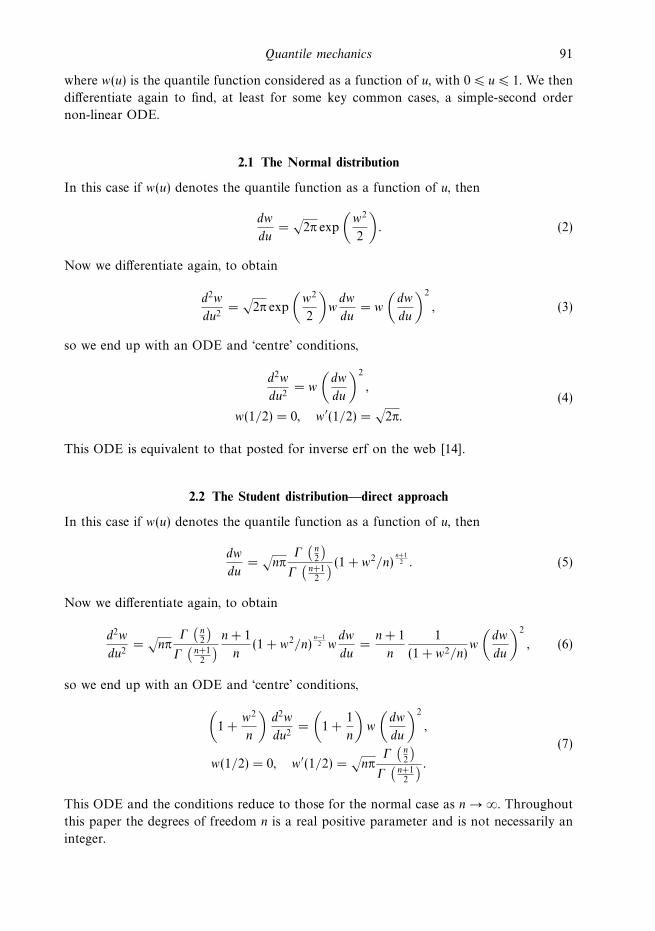
2.1 The Normal distribution
In this case if w(u) denotes the quantile function as a function of u, then
dw
du=
√2π exp
(w2
2
). (2)
Now we differentiate again, to obtain
d2w
du2=
√2π exp
(w2
2
)wdw
du= w
(dw
du
)2
, (3)
so we end up with an ODE and ‘centre’ conditions,
d2w
du2= w
(dw
du
)2
,(4)
w(1/2) = 0, w′(1/2) =√
2π.
This ODE is equivalent to that posted for inverse erf on the web [14].
2.2 The Student distribution—direct approach
In this case if w(u) denotes the quantile function as a function of u, then
dw
du=
√nπ
Γ(n2
)Γ
(n+12
) (1 + w2/n)n+12 . (5)
Now we differentiate again, to obtain
d2w
du2=
√nπ
Γ(n2
)Γ
(n+12
) n + 1
n(1 + w2/n)
n−12 w
dw
du=
n + 1
n
1
(1 + w2/n)w
(dw
du
)2
, (6)
so we end up with an ODE and ‘centre’ conditions,
(1 +
w2
n
)d2w
du2=
(1 +
1
n
)w
(dw
du
)2
,
(7)
w(1/2) = 0, w′(1/2) =√nπ
Γ(n2
)Γ
(n+12
) .This ODE and the conditions reduce to those for the normal case as n → ∞. Throughout
this paper the degrees of freedom n is a real positive parameter and is not necessarily an
integer.
92 G. Steinbrecher and W. T. Shaw
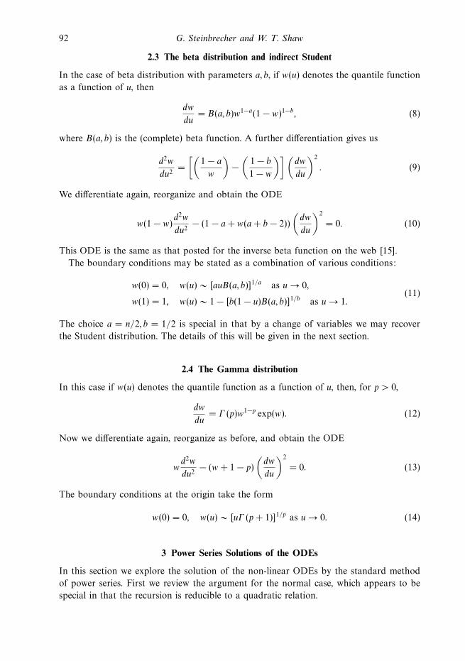
2.3 The beta distribution and indirect Student
In the case of beta distribution with parameters a, b, if w(u) denotes the quantile function
as a function of u, then
dw
du= B(a, b)w1−a(1 − w)1−b, (8)
where B(a, b) is the (complete) beta function. A further differentiation gives us
d2w
du2=
[(1 − a
w
)−
(1 − b
1 − w
)] (dw
du
)2
. (9)
We differentiate again, reorganize and obtain the ODE
w(1 − w)d2w
du2− (1 − a + w(a + b − 2))
(dw
du
)2
= 0. (10)
This ODE is the same as that posted for the inverse beta function on the web [15].
The boundary conditions may be stated as a combination of various conditions:
w(0) = 0, w(u) ∼ [auB(a, b)]1/a as u → 0,
w(1) = 1, w(u) ∼ 1 − [b(1 − u)B(a, b)]1/b as u → 1.(11)
The choice a = n/2, b = 1/2 is special in that by a change of variables we may recover
the Student distribution. The details of this will be given in the next section.
2.4 The Gamma distribution
In this case if w(u) denotes the quantile function as a function of u, then, for p > 0,
dw
du= Γ (p)w1−p exp(w). (12)
Now we differentiate again, reorganize as before, and obtain the ODE
wd2w
du2− (w + 1 − p)
(dw
du
)2
= 0. (13)
The boundary conditions at the origin take the form
w(0) = 0, w(u) ∼ [uΓ (p + 1)]1/p as u → 0. (14)
3 Power Series Solutions of the ODEs
In this section we explore the solution of the non-linear ODEs by the standard method
of power series. First we review the argument for the normal case, which appears to be
special in that the recursion is reducible to a quadratic relation.
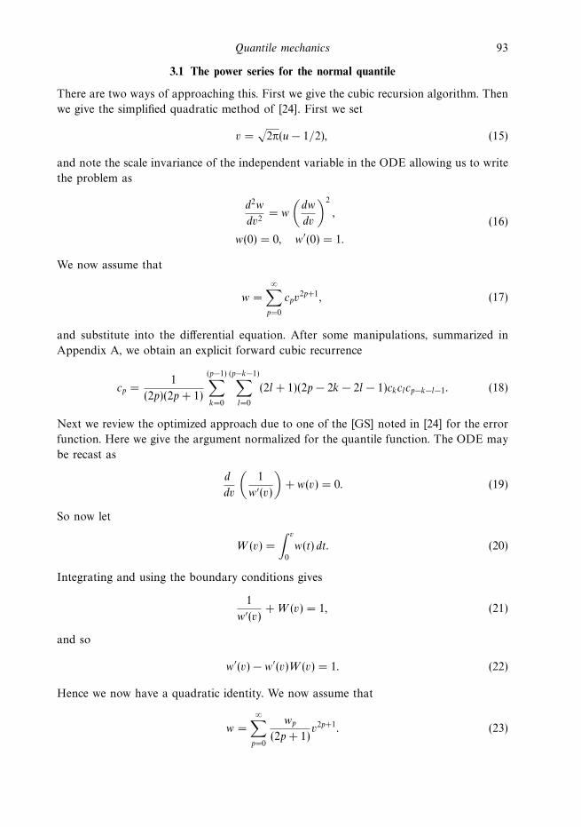
Quantile mechanics 93
3.1 The power series for the normal quantile
There are two ways of approaching this. First we give the cubic recursion algorithm. Then
we give the simplified quadratic method of [24]. First we set
v =√
2π(u − 1/2), (15)
and note the scale invariance of the independent variable in the ODE allowing us to write
the problem as
d2w
dv2= w
(dw
dv
)2
,
w(0) = 0, w′(0) = 1.
(16)
We now assume that
w =
∞∑p=0
cpv2p+1, (17)
and substitute into the differential equation. After some manipulations, summarized in
Appendix A, we obtain an explicit forward cubic recurrence
cp =1
(2p)(2p + 1)
(p−1)∑k=0
(p−k−1)∑l=0
(2l + 1)(2p − 2k − 2l − 1)ckclcp−k−l−1. (18)
Next we review the optimized approach due to one of the [GS] noted in [24] for the error
function. Here we give the argument normalized for the quantile function. The ODE may
be recast as
d
dv
(1
w′(v)
)+ w(v) = 0. (19)
So now let
W (v) =
∫ v
0
w(t) dt. (20)
Integrating and using the boundary conditions gives
1
w′(v)+ W (v) = 1, (21)
and so
w′(v) − w′(v)W (v) = 1. (22)
Hence we now have a quadratic identity. We now assume that
w =
∞∑p=0
wp
(2p + 1)v2p+1. (23)
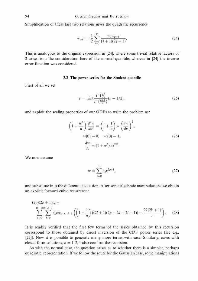
94 G. Steinbrecher and W. T. Shaw
Simplification of these last two relations gives the quadratic recurrence
wp+1 =1
2
p∑j=0
wjwp−j
(j + 1)(2j + 1). (24)
This is analogous to the original expression in [24], where some trivial relative factors of
2 arise from the consideration here of the normal quantile, whereas in [24] the inverse
error function was considered.
3.2 The power series for the Student quantile
First of all we set
v =√nπ
Γ(n2
)Γ
(n+12
) (u − 1/2), (25)
and exploit the scaling properties of our ODEs to write the problem as:
(1 +
w2
n
)d2w
dv2=
(1 +
1
n
)w
(dw
dv
)2
,
w(0) = 0, w′(0) = 1, (26)
dw
dv= (1 + w2/n)
n+12 .
We now assume
w =
∞∑p=0
cpv2p+1, (27)
and substitute into the differential equation. After some algebraic manipulations we obtain
an explicit forward cubic recurrence:
(2p)(2p + 1)cp =
(p−1)∑k=0
(p−k−1)∑l=0
ckclcp−k−l−1
((1 +
1
n
)((2l + 1)(2p − 2k − 2l − 1)) − 2k(2k + 1)
n
). (28)
It is readily verified that the first few terms of the series obtained by this recursion
correspond to those obtained by direct inversion of the CDF power series (see e.g.,
[22]). Now it is possible to generate many more terms with ease. Similarly, cases with
closed-form solutions, n = 1, 2, 4 also confirm the recursion.
As with the normal case, the question arises as to whether there is a simpler, perhaps
quadratic, representation. If we follow the route for the Gaussian case, some manipulations
Quantile mechanics 95
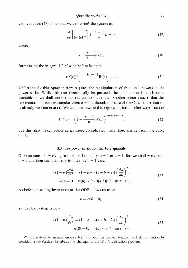
with equation (27) show that we can write1 the system as
d
dv
[1
(w′(v))α
]+
(n − 1)
nw = 0, (29)
where
α =(n − 1)
(n + 1)< 1. (30)
Introducing the integral W of w as before leads to
(w′(v))α[1 − (n − 1)
nW (v)
]= 1. (31)
Unfortunately this equation now requires the manipulation of fractional powers of the
power series. While this can theoretically be pursued, the cubic route is much more
tractable, so we shall confine our analysis to that route. Another minor issue is that this
representation becomes singular when n = 1, although this case of the Cauchy distribution
is already well understood. We can also rewrite this representation in other ways, such as
W ′′(v) =
(1 − (n − 1)
nW (v)
)−(n+1)/(n−1)
, (32)
but this also makes power series more complicated than those arising from the cubic
ODE.
3.3 The power series for the beta quantile
One can consider working from either boundary, u = 0 or u = 1. But we shall work from
u = 0 and then use symmetry to infer the u = 1 case.
w(1 − w)d2w
du2= (1 − a + w(a + b − 2))
(dw
du
)2
,
w(0) = 0, w(u) ∼ [auB(a, b)]1/a as u → 0.
(33)
As before, rescaling invariance of the ODE allows us to set
v = auB(a, b), (34)
so that the system is now
w(1 − w)d2w
dv2= (1 − a + w(a + b − 2))
(dw
dv
)2
,
w(0) = 0, w(u) ∼ v1/a as v → 0.
(35)
1We are grateful to an anonymous referee for pointing this out together with its motivation by
considering the Student distribution as the equilibrium of a fast diffusion problem.
96 G. Steinbrecher and W. T. Shaw
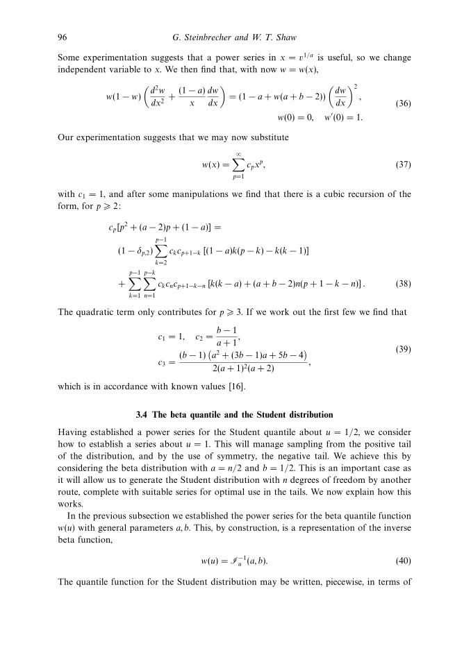
Some experimentation suggests that a power series in x = v1/a is useful, so we change
independent variable to x. We then find that, with now w = w(x),
w(1 − w)
(d2w
dx2+
(1 − a)
x
dw
dx
)= (1 − a + w(a + b − 2))
(dw
dx
)2
,
w(0) = 0, w′(0) = 1.
(36)
Our experimentation suggests that we may now substitute
w(x) =
∞∑p=1
cpxp, (37)
with c1 = 1, and after some manipulations we find that there is a cubic recursion of the
form, for p � 2:
cp[p2 + (a − 2)p + (1 − a)] =
(1 − δp,2)
p−1∑k=2
ckcp+1−k [(1 − a)k(p − k) − k(k − 1)]
+
p−1∑k=1
p−k∑n=1
ckcncp+1−k−n [k(k − a) + (a + b − 2)n(p + 1 − k − n)] . (38)
The quadratic term only contributes for p � 3. If we work out the first few we find that
c1 = 1, c2 =b − 1
a + 1,
c3 =(b − 1)
(a2 + (3b − 1)a + 5b − 4
)2(a + 1)2(a + 2)
,
(39)
which is in accordance with known values [16].
3.4 The beta quantile and the Student distribution
Having established a power series for the Student quantile about u = 1/2, we consider
how to establish a series about u = 1. This will manage sampling from the positive tail
of the distribution, and by the use of symmetry, the negative tail. We achieve this by
considering the beta distribution with a = n/2 and b = 1/2. This is an important case as
it will allow us to generate the Student distribution with n degrees of freedom by another
route, complete with suitable series for optimal use in the tails. We now explain how this
works.
In the previous subsection we established the power series for the beta quantile function
w(u) with general parameters a, b. This, by construction, is a representation of the inverse
beta function,
w(u) = I−1u (a, b). (40)
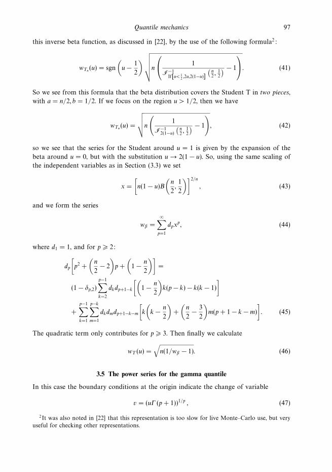
The quantile function for the Student distribution may be written, piecewise, in terms of
Quantile mechanics 97
this inverse beta function, as discussed in [22], by the use of the following formula2:
wTn(u) = sgn
(u − 1
2
)√√√√√n
⎛⎝ 1
I−1If[u< 1
2 ,2u,2(1−u)]
(n2, 1
2
) − 1
⎞⎠. (41)
So we see from this formula that the beta distribution covers the Student T in two pieces,
with a = n/2, b = 1/2. If we focus on the region u > 1/2, then we have
wTn(u) =
√√√√n
(1
I−12(1−u)
(n2, 1
2
) − 1
), (42)
so we see that the series for the Student around u = 1 is given by the expansion of the
beta around u = 0, but with the substitution u → 2(1 − u). So, using the same scaling of
the independent variables as in Section (3.3) we set
x =
[n(1 − u)B
(n
2,1
2
)]2/n
, (43)
and we form the series
wβ =
∞∑p=1
dpxp, (44)
where d1 = 1, and for p � 2:
dp
[p2 +
(n
2− 2
)p +
(1 − n
2
)]=
(1 − δp,2)
p−1∑k=2
dkdp+1−k
[(1 − n
2
)k(p − k) − k(k − 1)
]
+
p−1∑k=1
p−k∑m=1
dkdmdp+1−k−m
[k
(k − n
2
)+
(n
2− 3
2
)m(p + 1 − k − m)
]. (45)
The quadratic term only contributes for p � 3. Then finally we calculate
wT (u) =√n(1/wβ − 1). (46)
3.5 The power series for the gamma quantile
In this case the boundary conditions at the origin indicate the change of variable
v = (uΓ (p + 1))1/p , (47)
2It was also noted in [22] that this representation is too slow for live Monte–Carlo use, but very
useful for checking other representations.
98 G. Steinbrecher and W. T. Shaw
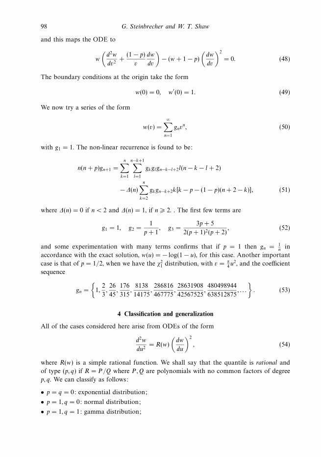
and this maps the ODE to
w
(d2w
dv2+
(1 − p)
v
dw
dv
)− (w + 1 − p)
(dw
dv
)2
= 0. (48)
The boundary conditions at the origin take the form
w(0) = 0, w′(0) = 1. (49)
We now try a series of the form
w(v) =
∞∑n=1
gnvn, (50)
with g1 = 1. The non-linear recurrence is found to be:
n(n + p)gn+1 =
n∑k=1
n−k+1∑l=1
gkglgn−k−l+2l(n − k − l + 2)
−∆(n)
n∑k=2
gkgn−k+2k[k − p − (1 − p)(n + 2 − k)], (51)
where ∆(n) = 0 if n < 2 and ∆(n) = 1, if n � 2. . The first few terms are
g1 = 1, g2 =1
p + 1, g3 =
3p + 5
2(p + 1)2(p + 2), (52)
and some experimentation with many terms confirms that if p = 1 then gn = 1n
in
accordance with the exact solution, w(u) = − log(1 − u), for this case. Another important
case is that of p = 1/2, when we have the χ21 distribution, with v = π
4u2, and the coefficient
sequence
gn =
{1,
2
3,26
45,176
315,
8138
14175,286816
467775,28631908
42567525,480498944
638512875, . . .
}. (53)
4 Classification and generalization
All of the cases considered here arise from ODEs of the form
d2w
du2= R(w)
(dw
du
)2
, (54)
where R(w) is a simple rational function. We shall say that the quantile is rational and
of type (p, q) if R = P/Q where P ,Q are polynomials with no common factors of degree
p, q. We can classify as follows:
• p = q = 0: exponential distribution;
• p = 1, q = 0: normal distribution;
• p = 1, q = 1: gamma distribution;
Quantile mechanics 99
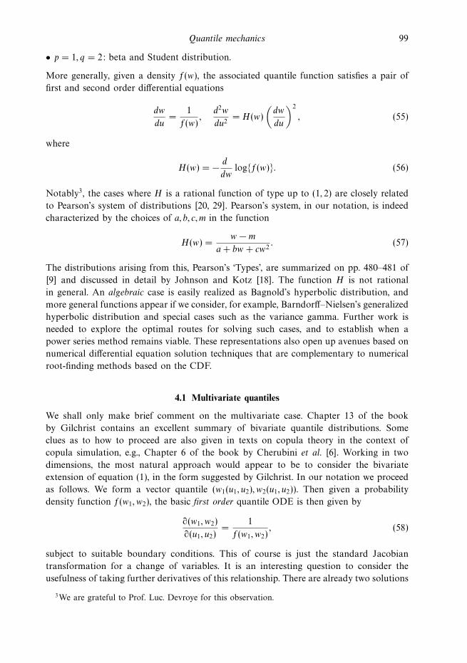
• p = 1, q = 2: beta and Student distribution.
More generally, given a density f(w), the associated quantile function satisfies a pair of
first and second order differential equations
dw
du=
1
f(w),
d2w
du2= H(w)
(dw
du
)2
, (55)
where
H(w) = − d
dwlog{f(w)}. (56)
Notably3, the cases where H is a rational function of type up to (1, 2) are closely related
to Pearson’s system of distributions [20, 29]. Pearson’s system, in our notation, is indeed
characterized by the choices of a, b, c, m in the function
H(w) =w − m
a + bw + cw2. (57)
The distributions arising from this, Pearson’s ‘Types’, are summarized on pp. 480–481 of
[9] and discussed in detail by Johnson and Kotz [18]. The function H is not rational
in general. An algebraic case is easily realized as Bagnold’s hyperbolic distribution, and
more general functions appear if we consider, for example, Barndorff–Nielsen’s generalized
hyperbolic distribution and special cases such as the variance gamma. Further work is
needed to explore the optimal routes for solving such cases, and to establish when a
power series method remains viable. These representations also open up avenues based on
numerical differential equation solution techniques that are complementary to numerical
root-finding methods based on the CDF.
4.1 Multivariate quantiles
We shall only make brief comment on the multivariate case. Chapter 13 of the book
by Gilchrist contains an excellent summary of bivariate quantile distributions. Some
clues as to how to proceed are also given in texts on copula theory in the context of
copula simulation, e.g., Chapter 6 of the book by Cherubini et al. [6]. Working in two
dimensions, the most natural approach would appear to be to consider the bivariate
extension of equation (1), in the form suggested by Gilchrist. In our notation we proceed
as follows. We form a vector quantile (w1(u1, u2), w2(u1, u2)). Then given a probability
density function f(w1, w2), the basic first order quantile ODE is then given by
∂(w1, w2)
∂(u1, u2)=
1
f(w1, w2), (58)
subject to suitable boundary conditions. This of course is just the standard Jacobian
transformation for a change of variables. It is an interesting question to consider the
usefulness of taking further derivatives of this relationship. There are already two solutions
3We are grateful to Prof. Luc. Devroye for this observation.
100 G. Steinbrecher and W. T. Shaw
to equation (58) in the case of the normal distribution that are implicit in well-known
bivariate simulation methods. For example, setting
w1(u1, u2) = w0(u1), w2(u1, u2) = w0(u2)√
1 − ρ2 + ρw0(u1), (59)
gives us a solution of equation (58), where w0 is the quantile of the normal distribution,
and f is given by
f(w1, w2) =1
2π√
1 − ρ2exp
{− 1
2(1 − ρ2)
(w2
1 + w22 − 2ρw1w2
)}. (60)
The construction of the bivariate normal based on a pair of univariate quantiles with the
Box–Muller simulation method, as discussed in Section 7.3.4 of [21], also gives a solution
of equation (58) in the independent case. In our notation the Box–Muller formula can be
considered as:
w1(u1, u2) =√
−2 log(u1) cos(2πu2), w2(u1, u2) =√
−2 log(u1) sin(2πu2), (61)
and correlated variables may be generated by superposition. So we can build two quite
different mappings from the unit square to the bivariate normal. In general, multivariate
and non-normal case, quantiles cannot of course be built up by such elementary super-
position. We also refer the reader to [21] for an introduction to modern methods not
employing quantiles, notably the ‘ratio of uniforms’ approach.
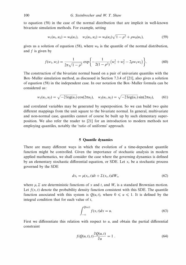
5 Quantile dynamics
There are many different ways in which the evolution of a time-dependent quantile
function might be controlled. Given the importance of stochastic analysis in modern
applied mathematics, we shall consider the case where the governing dynamics is defined
by an elementary stochastic differential equation, or SDE. Let xt be a stochastic process
governed by the SDE
dxt = µ(xt, t)dt + Σ(xt, t)dWt, (62)
where µ, Σ are deterministic functions of x and t, and Wt is a standard Brownian motion.
Let f(x, t) denote the probability density function consistent with this SDE. The quantile
function associated with this system is Q(u, t), where 0 � u � 1. It is defined by the
integral condition that for each value of t,
∫ Q(u,t)
−∞f(x, t)dx = u. (63)
First we differentiate this relation with respect to u, and obtain the partial differential
constraint
f(Q(u, t), t)∂Q(u, t)
∂u= 1 . (64)

Quantile mechanics 101
We differentiate this relation again, and obtain the following second order PDE,
∂f(Q(u, t), t)
∂Q
(∂Q(u, t)
∂u
)2
+ f(Q(u, t), t)∂2Q(u, t)
∂u2= 0. (65)
This may be reorganized into the equation
∂2Q(u, t)
∂u2= −∂ log(f(Q(u, t), t))
∂Q
(∂Q(u, t)
∂u
)2
. (66)
In the case of no time dependence, this is readily recognized as the second order non-
linear ODE derived and solved previously. In the time-dependent case we go back to the
condition of equation (63) and now differentiate with respect to time. The fundamental
theorem of calculus gives, first,
f(Q(u, t), t)∂Q
∂t+
∫ Q(u,t)
−∞
∂f(x, t)
∂tdx = 0. (67)
We use equation (64) to write this as:
∂Q
∂t= −∂Q
∂u
∫ Q(u,t)
−∞
∂f(x, t)
∂tdx. (68)
Next we use the Fokker–Planck (forward Kolmogorov) equation in the form [10]
∂f(x, t)
∂t=
∂
∂x
[−µf +
1
2
∂
∂x(Σ2f)
], (69)
where Σ is the volatility defined in the SDE of equation (62), and observe that we can do
the integration directly, and obtain the following:
∂Q
∂t= −∂Q
∂u
[−µ(Q, t)f(Q, t) +
1
2
(Σ2(Q, t)
∂f
∂Q+ f
∂Σ2(Q, t)
∂Q
)]. (70)
Finally we use our previous equations (64)–(65) to eliminate f and its derivative completely,
leaving us with
∂Q
∂t= µ(Q, t) − 1
2
∂Σ2
∂Q+
Σ2(Q, t)
2
(∂Q
∂u
)−2∂2Q
∂u2. (71)
This is the quantilized Fokker–Planck equation, or QFPE for short, associated with the
SDE of equation (62). It is a non-linear PDE, and is the form of the Carrillo-Toscani
equation [5] appropriate to solutions of an SDE.
5.1 Elementary solutions of the QFPE
Despite its non-linearities, we known that the QFPE of equation (71) must have some
elementary Gaussian solutions that will now be verified. First we explore the QFPE for
arithmetical Brownian motion. In this case we have µ and Σ constant and it is easy to
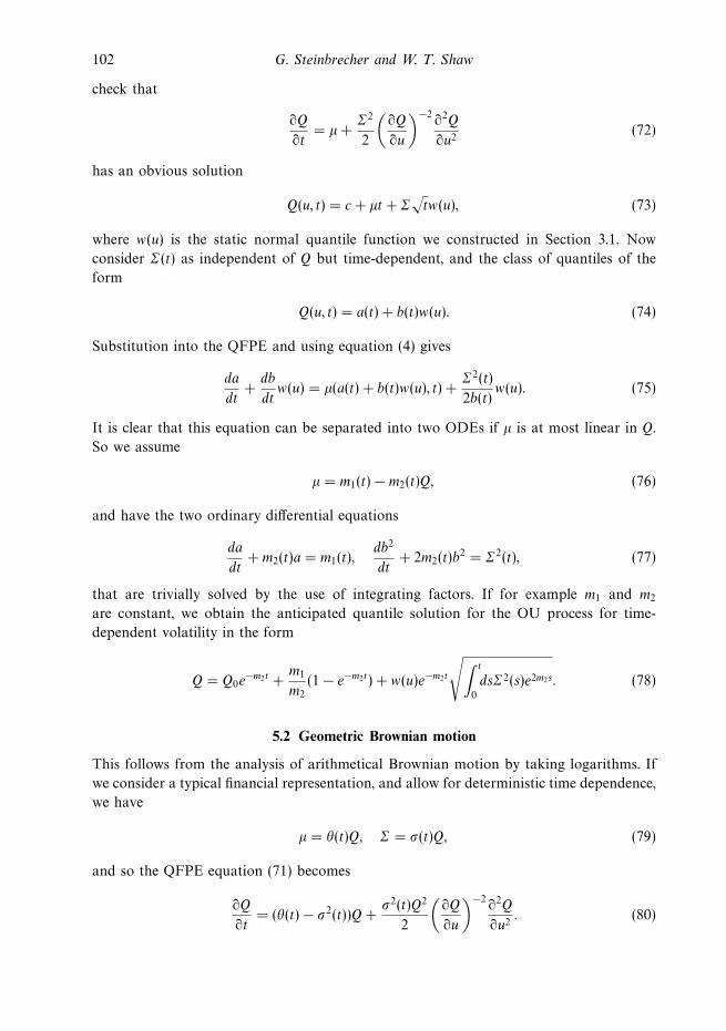
102 G. Steinbrecher and W. T. Shaw
check that
∂Q
∂t= µ +
Σ2
2
(∂Q
∂u
)−2∂2Q
∂u2(72)
has an obvious solution
Q(u, t) = c + µt + Σ√tw(u), (73)
where w(u) is the static normal quantile function we constructed in Section 3.1. Now
consider Σ(t) as independent of Q but time-dependent, and the class of quantiles of the
form
Q(u, t) = a(t) + b(t)w(u). (74)
Substitution into the QFPE and using equation (4) gives
da
dt+
db
dtw(u) = µ(a(t) + b(t)w(u), t) +
Σ2(t)
2b(t)w(u). (75)
It is clear that this equation can be separated into two ODEs if µ is at most linear in Q.
So we assume
µ = m1(t) − m2(t)Q, (76)
and have the two ordinary differential equations
da
dt+ m2(t)a = m1(t),
db2
dt+ 2m2(t)b
2 = Σ2(t), (77)
that are trivially solved by the use of integrating factors. If for example m1 and m2
are constant, we obtain the anticipated quantile solution for the OU process for time-
dependent volatility in the form
Q = Q0e−m2t +
m1
m2(1 − e−m2t) + w(u)e−m2t
√∫ t
0
dsΣ2(s)e2m2s. (78)
5.2 Geometric Brownian motion
This follows from the analysis of arithmetical Brownian motion by taking logarithms. If
we consider a typical financial representation, and allow for deterministic time dependence,
we have
µ = θ(t)Q, Σ = σ(t)Q, (79)
and so the QFPE equation (71) becomes
∂Q
∂t= (θ(t) − σ2(t))Q +
σ2(t)Q2
2
(∂Q
∂u
)−2∂2Q
∂u2. (80)
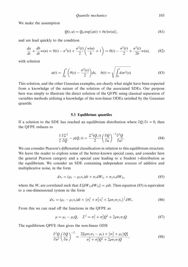
Quantile mechanics 103
We make the assumption
Q(t, u) = Q0 exp{a(t) + b(t)w(u)}, (81)
and are lead quickly to the condition
da
dt+
db
dtw(u) = θ(t) − σ2(t) +
σ2(t)
2
(w(u)
b+ 1
)= θ(t) − σ2(t)
2+
σ2(t)
2bw(u), (82)
with solution
a(t) =
∫ t
0
(θ(s) − σ2(s)
2
)ds, b(t) =
√∫ t
0
dsσ2(s). (83)
This solution, and the other Gaussian examples, are clearly what might have been expected
from a knowledge of the nature of the solution of the associated SDEs. Our purpose
here was simply to illustrate the direct solution of the QFPE using classical separation of
variables methods utilizing a knowledge of the non-linear ODEs satisfied by the Gaussian
quantile.
5.3 Equilibrium quantiles
If a solution to the SDE has reached an equilibrium distribution where ∂Q/∂t = 0, then
the QFPE reduces to
1
2
∂Σ2
∂Q− µ(Q, t) =
Σ2(Q, t)
2
(∂Q
∂u
)−2∂2Q
∂u2. (84)
We can consider Pearson’s differential classification in relation to this equilibrium structure.
We leave the reader to explore some of the better-known special cases, and consider here
the general Pearson category and a special case leading to a Student t-distribution as
the equilibrium. We consider an SDE containing independent sources of additive and
multiplicative noise, in the form
dxt = (µ1 − µ2xt)dt + σ1dW1t + σ2xtdW2t, (85)
where the Wi are correlated such that E[dW1tdW2t] = ρdt. Then equation (85) is equivalent
to a one-dimensional system in the form
dxt = (µ1 − µ2xt)dt +(σ2
1 + σ22x
2t + 2ρσ1σ2xt
) 12 dWt. (86)
From this we can read off the functions in the QFPE as
µ = µ1 − µ2Q, Σ2 = σ21 + σ2
2Q2 + 2ρσ1σ2Q. (87)
The equilibrium QPFE then gives the non-linear ODE
∂2Q
∂u2
(∂Q
∂u
)−2
=2[(ρσ1σ2 − µ1) +
(σ2
2 + µ2
)Q]
σ21 + σ2
2Q2 + 2ρσ1σ2Q
, (88)
104 G. Steinbrecher and W. T. Shaw
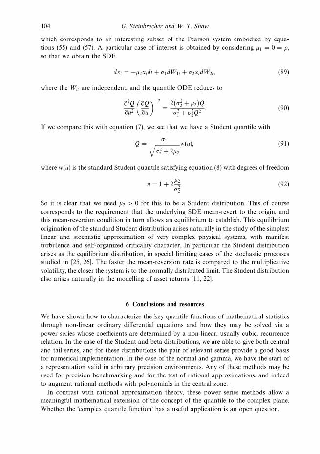
which corresponds to an interesting subset of the Pearson system embodied by equa-
tions (55) and (57). A particular case of interest is obtained by considering µ1 = 0 = ρ,
so that we obtain the SDE
dxt = −µ2xtdt + σ1dW1t + σ2xtdW2t, (89)
where the Wit are independent, and the quantile ODE reduces to
∂2Q
∂u2
(∂Q
∂u
)−2
=2(σ2
2 + µ2
)Q
σ21 + σ2
2Q2
. (90)
If we compare this with equation (7), we see that we have a Student quantile with
Q =σ1√
σ22 + 2µ2
w(u), (91)
where w(u) is the standard Student quantile satisfying equation (8) with degrees of freedom
n = 1 + 2µ2
σ22
. (92)
So it is clear that we need µ2 > 0 for this to be a Student distribution. This of course
corresponds to the requirement that the underlying SDE mean-revert to the origin, and
this mean-reversion condition in turn allows an equilibrium to establish. This equilibrium
origination of the standard Student distribution arises naturally in the study of the simplest
linear and stochastic approximation of very complex physical systems, with manifest
turbulence and self-organized criticality character. In particular the Student distribution
arises as the equilibrium distribution, in special limiting cases of the stochastic processes
studied in [25, 26]. The faster the mean-reversion rate is compared to the multiplicative
volatility, the closer the system is to the normally distributed limit. The Student distribution
also arises naturally in the modelling of asset returns [11, 22].
6 Conclusions and resources
We have shown how to characterize the key quantile functions of mathematical statistics
through non-linear ordinary differential equations and how they may be solved via a
power series whose coefficients are determined by a non-linear, usually cubic, recurrence
relation. In the case of the Student and beta distributions, we are able to give both central
and tail series, and for these distributions the pair of relevant series provide a good basis
for numerical implementation. In the case of the normal and gamma, we have the start of
a representation valid in arbitrary precision environments. Any of these methods may be
used for precision benchmarking and for the test of rational approximations, and indeed
to augment rational methods with polynomials in the central zone.
In contrast with rational approximation theory, these power series methods allow a
meaningful mathematical extension of the concept of the quantile to the complex plane.
Whether the ‘complex quantile function’ has a useful application is an open question.
Quantile mechanics 105
We have also considered the non-linear integrated form of the Fokker–Planck equation,
as introduced by Carrillo and Toscani [5], and demonstrated how the resulting non-linear
PDE may be solved in some cases of interest.
6.1 Internet resources
Our intention is to provide a growing list of links to on line computational resources
for the implementation of these and related methods. Some links are provided in the
references. Specific discussions are also available as follows in Mathematica, C++ and
Fortran 95. These will evolve as our knowledge about optimal implementations grows.
• A Mathematica file with investigations of some these methods is at:
http://www.mth.kcl.ac.uk/~shaww/web page/papers/quantiles/
QuantileDemos.nb
• C++ code for the central normal power series is at:
http://www.mth.kcl.ac.uk/~shaww/web_page/papers/quantiles/
normalquantile.cpp
• Quad precision F95 code for the central normal power series is at:
http://www.mth.kcl.ac.uk/~shaww/web_page/papers/quantiles/
normalquantile.f95
• Quad precision F95 code for the Student case (central & tail) is at:
http://www.mth.kcl.ac.uk/~shaww/web_page/papers/quantiles/
studentquantile.f95
In addition a web page is being maintained with further examples and related art-
icle, with the entry point at http://www.mth.kcl.ac.uk/~shaww/web page/papers/
quantiles/Quantiles.htm
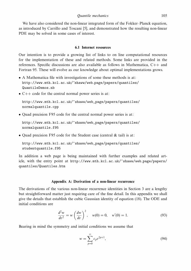
Appendix A: Derivation of a non-linear recurrence
The derivations of the various non-linear recurrence identities in Section 3 are a lengthy
but straightforward matter just requiring care of the fine detail. In this appendix we shall
give the details that establish the cubic Gaussian identity of equation (18). The ODE and
initial conditions are
d2w
dv2= w
(dw
dv
)2
, w(0) = 0, w′(0) = 1. (93)
Bearing in mind the symmetry and initial conditions we assume that
w =
∞∑p=0
cpv2p+1, (94)
106 G. Steinbrecher and W. T. Shaw
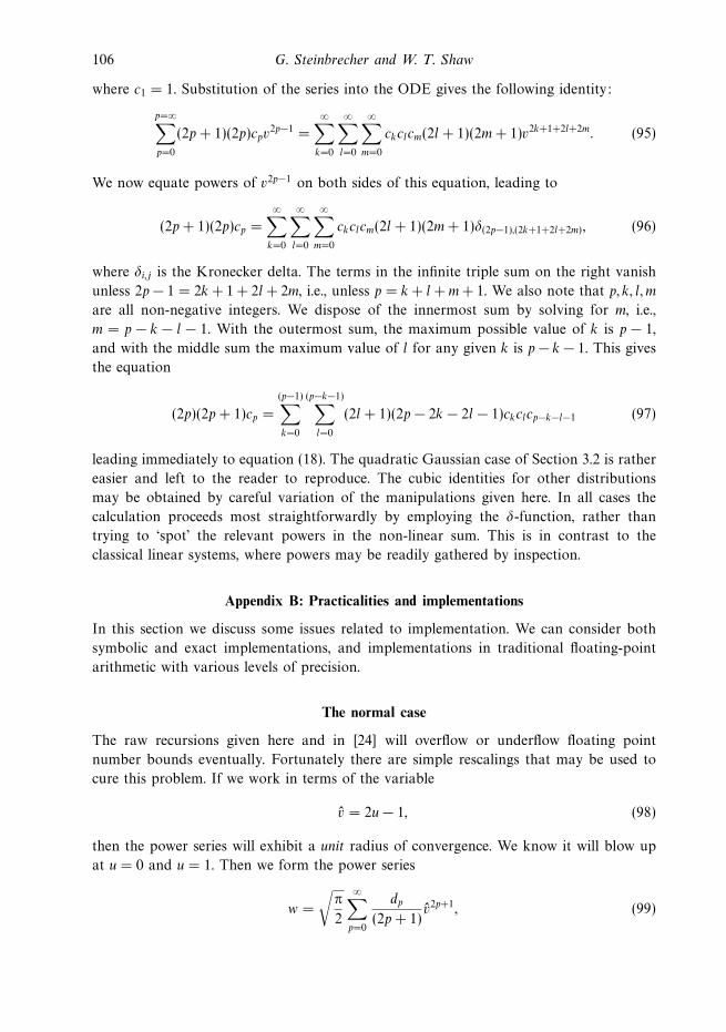
where c1 = 1. Substitution of the series into the ODE gives the following identity:
p=∞∑p=0
(2p + 1)(2p)cpv2p−1 =
∞∑k=0
∞∑l=0
∞∑m=0
ckclcm(2l + 1)(2m + 1)v2k+1+2l+2m. (95)
We now equate powers of v2p−1 on both sides of this equation, leading to
(2p + 1)(2p)cp =
∞∑k=0
∞∑l=0
∞∑m=0
ckclcm(2l + 1)(2m + 1)δ(2p−1),(2k+1+2l+2m), (96)
where δi,j is the Kronecker delta. The terms in the infinite triple sum on the right vanish
unless 2p − 1 = 2k + 1 + 2l + 2m, i.e., unless p = k + l +m+ 1. We also note that p, k, l, m
are all non-negative integers. We dispose of the innermost sum by solving for m, i.e.,
m = p − k − l − 1. With the outermost sum, the maximum possible value of k is p − 1,
and with the middle sum the maximum value of l for any given k is p − k − 1. This gives
the equation
(2p)(2p + 1)cp =
(p−1)∑k=0
(p−k−1)∑l=0
(2l + 1)(2p − 2k − 2l − 1)ckclcp−k−l−1 (97)
leading immediately to equation (18). The quadratic Gaussian case of Section 3.2 is rather
easier and left to the reader to reproduce. The cubic identities for other distributions
may be obtained by careful variation of the manipulations given here. In all cases the
calculation proceeds most straightforwardly by employing the δ-function, rather than
trying to ‘spot’ the relevant powers in the non-linear sum. This is in contrast to the
classical linear systems, where powers may be readily gathered by inspection.
Appendix B: Practicalities and implementations
In this section we discuss some issues related to implementation. We can consider both
symbolic and exact implementations, and implementations in traditional floating-point
arithmetic with various levels of precision.
The normal case
The raw recursions given here and in [24] will overflow or underflow floating point
number bounds eventually. Fortunately there are simple rescalings that may be used to
cure this problem. If we work in terms of the variable
v = 2u − 1, (98)
then the power series will exhibit a unit radius of convergence. We know it will blow up
at u = 0 and u = 1. Then we form the power series
w =
√π
2
∞∑p=0
dp
(2p + 1)v2p+1, (99)

Quantile mechanics 107
with d0 = 1. In terms of these variables the quadratic recurrence becomes
dp+1 =π
4
p∑j=0
djdp−j
(j + 1)(2j + 1). (100)
With such a scheme the ratio dp+1/dp → 1 as p → ∞, and numerical implementations
confirm this. The limits of how far the series can be taken are then just a matter of
computation time. The second observation is that the sum involves the product djdp−j
twice, so that one can optimize by summing half-way and taking care to note whether p
is odd or even. The recurrence can be written
dp+1 =π
4
� p−12 �∑
j=0
djdp−j
(1
(j + 1)(2j + 1)+
1
(p − j + 1)(2p − 2j + 1)
)
+ If(p is even,π
4
d2p2(
p2
+ 1)(p + 1)
, else 0). (101)
In our initial implementations of the normal case in C++ and F95, attention has been
confined to the central power series, and with very simple series termination criteria, in-
volving termination when the next term to be computed falls below a certain level. While
this is appropriate in a rigorous sense for alternating series, it is a temporary solution
for monotone series such as those that are being considered here. The resulting error
characteristics are nevertheless encouraging, and we can cover a large proportion of the
unit interval with a precision that is more dependent on hardware and compiler choices
than on the algorithm itself. In C++ the level of precision achievable depends on the
quality of the implementation of the ‘long double’ data type. This is not, regrettably, rig-
orously specified in the C++ standard. The demonstration C++ code cited in Section 6.1
works on 0.0005 < u < 0.9995 with maximum relative error less than 1.7 × 10⁻¹⁵ and on
0.0035 < u < 0.9965 with maximum relative error less than 2.5 × 10⁻¹⁶, when using the
Bloodshed Dev C++ under Windows XP on a Pentium M. Results with other hardware
and/or compilers will vary, especially if a poor long double implementation is used. For
a more controlled implementation, we turn to quadruple precision Fortran 95. Using the
Absoft compiler for MacOS on Intel, we obtained a relative error less than 10−29 on
the interval 0.0007 < u < 0.9993. All precision calculations were assessed by reference
to the inverse error function built in to Mathematica 5.2, using 40 significant figures for
the calculations. We stress that such code is not necessarily fast enough to use in live
Monte–Carlo simulation, but, at this stage in the development, is more appropriately
viewed as a means for benchmarking a new class of fast rational approximations.
The Student case
In this case we have a pair of power series for central and tail use and we may proceed
directly to an implementation. One issue that has to be dealt with is the computation of
the rescaling factor in the formula of equation (25), which we write as
v =
√nπ
2
Γ ( n2)
Γ(n+12
) (2u − 1) = γn(2u − 1). (102)
108 G. Steinbrecher and W. T. Shaw
We use the identity
γn+2 =
√n(n + 2)
n + 1γn (103)
to simplify the high-precision computation of this quantity. When n is an integer with
n � 10 we use a precomputed value of γn. When n is a larger integer we recurse down to
9 or 10. When n is non-integer we recurse up to a value larger than 1000 and then apply
the result that as n → ∞, γn
√2π
is asymptotic to
1 +1
4n+
1
32n2− 5
128n3− 21
2048n4+
399
8192n5+
869
65536n6− 39325
262144n7− 334477
8388608n8
+28717403
33554432n9+
59697183
268435456n10− 8400372435
1073741824n11− 34429291905
17179869184n12. (104)
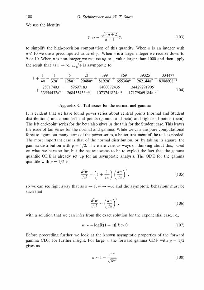
Appendix C: Tail issues for the normal and gamma
It is evident that we have found power series about central points (normal and Student
distributions) and about left end points (gamma and beta) and right end points (beta).
The left end-point series for the beta also gives us the tails for the Student case. This leaves
the issue of tail series for the normal and gamma. While we can use pure computational
force to figure out many terms of the power series, a better treatment of the tails is needed.
The most important case is that of the normal distribution, or, by taking its square, the
gamma distribution with p = 1/2. There are various ways of thinking about this, based
on what we have so far, but the neatest seems to be to exploit the fact that the gamma
quantile ODE is already set up for an asymptotic analysis. The ODE for the gamma
quantile with p = 1/2 is
d2w
du2=
(1 +
1
2w
)(dw
du
)2
, (105)
so we can see right away that as u → 1, w → +∞ and the asymptotic behaviour must be
such that
d2w
du2∼
(dw
du
)2
, (106)
with a solution that we can infer from the exact solution for the exponential case, i.e.,
w ∼ − log[k(1 − u)], k > 0. (107)
Before proceeding further we look at the known asymptotic properties of the forward
gamma CDF, for further insight. For large w the forward gamma CDF with p = 1/2
gives us
u ∼ 1 − e−w
√πw
, (108)
Quantile mechanics 109
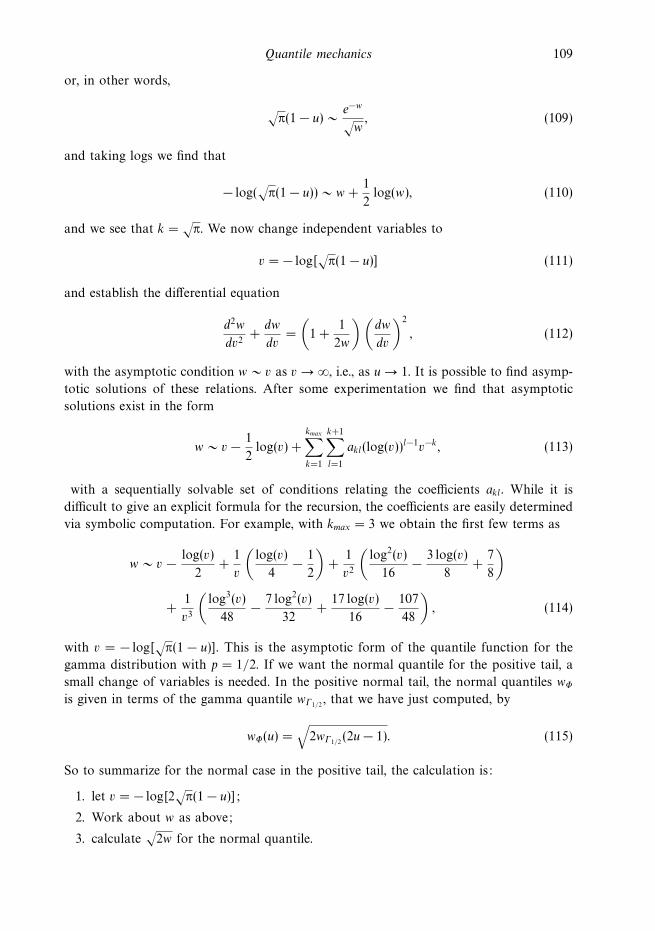
or, in other words,
√π(1 − u) ∼ e−w
√w, (109)
and taking logs we find that
− log(√
π(1 − u)) ∼ w +1
2log(w), (110)
and we see that k =√
π. We now change independent variables to
v = − log[√
π(1 − u)] (111)
and establish the differential equation
d2w
dv2+
dw
dv=
(1 +
1
2w
)(dw
dv
)2
, (112)
with the asymptotic condition w ∼ v as v → ∞, i.e., as u → 1. It is possible to find asymp-
totic solutions of these relations. After some experimentation we find that asymptotic
solutions exist in the form
w ∼ v − 1
2log(v) +
kmax∑k=1
k+1∑l=1
akl(log(v))l−1v−k, (113)
with a sequentially solvable set of conditions relating the coefficients akl . While it is
difficult to give an explicit formula for the recursion, the coefficients are easily determined
via symbolic computation. For example, with kmax = 3 we obtain the first few terms as
w ∼ v − log(v)
2+
1
v
(log(v)
4− 1
2
)+
1
v2
(log2(v)
16− 3 log(v)
8+
7
8
)
+1
v3
(log3(v)
48− 7 log2(v)
32+
17 log(v)
16− 107
48
), (114)
with v = − log[√
π(1 − u)]. This is the asymptotic form of the quantile function for the
gamma distribution with p = 1/2. If we want the normal quantile for the positive tail, a
small change of variables is needed. In the positive normal tail, the normal quantiles wΦ
is given in terms of the gamma quantile wΓ1/2, that we have just computed, by
wΦ(u) =√
2wΓ1/2(2u − 1). (115)
So to summarize for the normal case in the positive tail, the calculation is:
1. let v = − log[2√
π(1 − u)];
2. Work about w as above;
3. calculate√
2w for the normal quantile.
110 G. Steinbrecher and W. T. Shaw
k Order 3 asymp Mathematica AS241 Excel
3 3.089631766 3.090232306 3.090232306 3.090232306
4 3.718896182 3.719016485 3.719016485 3.719016485
5 4.264854901 4.264890794 4.264890794 4.264890794
6 4.753410708 4.753424309 4.753424309 4.753424341
7 5.199331535 5.199337582 5.199337582 5.199337618
8 5.611998229 5.612001244 5.612001244 5.612001258
9 5.997805376 5.997807015 5.997807015 5.997807018
10 6.361339949 6.361340902 6.361340902 6.361340808
11 6.706022570 6.706023155 6.706023155 6.706022335
12 7.034483450 7.034483825 7.034483825 7.034479171
13 7.348795853 7.348796103 7.348796103 7.348680374
14 7.650627921 7.650628093 7.650628093 7.650018522
15 7.941345205 7.941345326 7.941345326 7.934736689
16 8.222082128 8.222082216 8.222082216 NA
17 8.493793159 8.493793224 8.493793224 NA
18 8.757290300 8.757290349 8.757290349 NA
19 9.013271116 9.013271153 9.013271153 NA
20 9.262340061 9.262340090 9.262340090 NA
21 9.505024960 9.505024983 9.505024983 NA
22 9.741789925 9.741789943 9.741789943 NA
23 9.973045605 9.973045620 9.973045620 NA
24 10.19915741 10.19915742 10.19915742 NA
25 10.42045219 10.42045220 10.42045220 NA
26 10.63722367 10.63722368 10.63722368 NA
27 10.84973699 10.84973700 10.84973700 NA
28 11.05823241 11.05823241 11.05823241 NA
29 11.26292848 11.26292848 11.26292848 NA
30 11.46402468 11.46402469 11.46402469 NA
31 11.66170368 11.66170368 11.66170368 NA
32 11.85613321 11.85613322 11.85613322 NA
33 12.04746778 12.04746779 12.04746779 NA
34 12.23585004 12.23585005 12.23585005 NA
35 12.42141204 12.42141204 12.42141204 NA
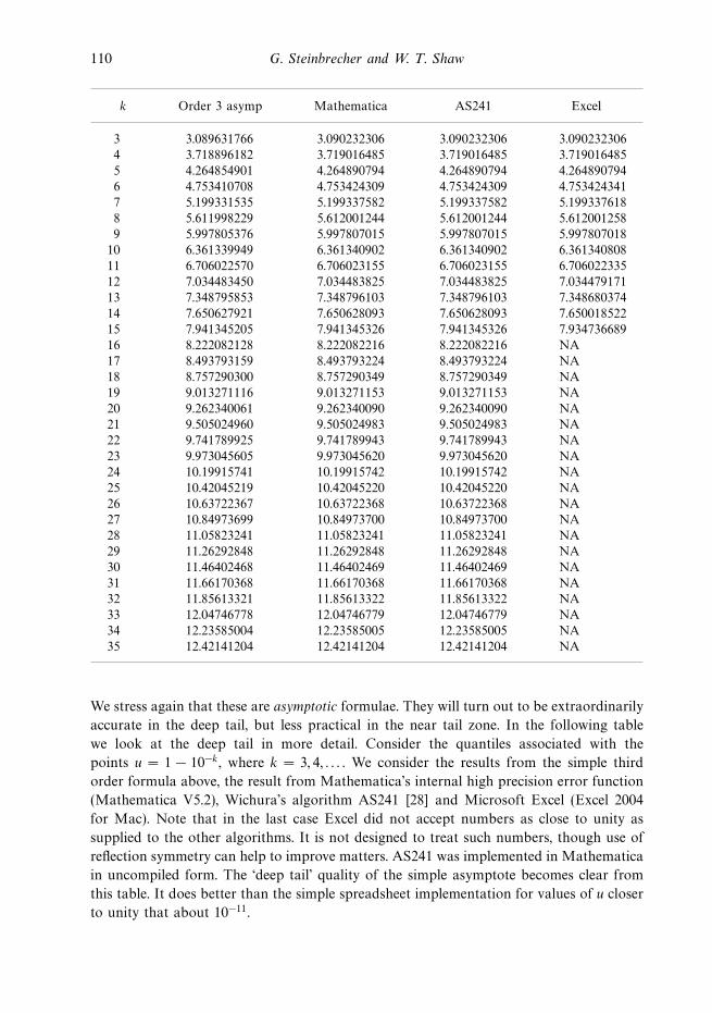
We stress again that these are asymptotic formulae. They will turn out to be extraordinarily
accurate in the deep tail, but less practical in the near tail zone. In the following table
we look at the deep tail in more detail. Consider the quantiles associated with the
points u = 1 − 10−k , where k = 3, 4, . . . . We consider the results from the simple third
order formula above, the result from Mathematica’s internal high precision error function
(Mathematica V5.2), Wichura’s algorithm AS241 [28] and Microsoft Excel (Excel 2004
for Mac). Note that in the last case Excel did not accept numbers as close to unity as
supplied to the other algorithms. It is not designed to treat such numbers, though use of
reflection symmetry can help to improve matters. AS241 was implemented in Mathematica
in uncompiled form. The ‘deep tail’ quality of the simple asymptote becomes clear from
this table. It does better than the simple spreadsheet implementation for values of u closer
to unity that about 10−11.
Quantile mechanics 111
Acknowledgements
We wish to thank Prof. L Devroye for his comment on the Pearson classification, and
Prof. W. Gilchrist for several useful remarks. Our understanding of the history of the
approaches to quantiles has benefited from comments by Dr. A. Dassios, Prof. G. Toscani
and Prof. N. Bingham. William Shaw wishes to thank Absoft Corporation for their help
on quadruple precision Fortran. The Fortran 95 associated with this work was developed
and tested with the Absoft Fortran for MacOS on Intel compiler. The C++ code was
developed with the Bloodshed Dev C++ compiler. We also thank our anonymous referees
for several suggestions for revision to an earlier draft of this paper.
References
[1] Abernathy, R. W. & Smith, R. P. (1993) Applying series expansion to the inverse beta
distribution to find percentiles of the F-distribution. ACM Tran. Math. Soft. 19(4), 474–480.
[2] Acklam, P. J. An algorithm for computing the inverse normal cumulative distribution function,
http://home.online.no/~pjacklam/notes/invnorm/
[3] Aletti, G., Naldi, G. & Toscani, G. (2007) First-order continuous models of opinion forma-
tion, SIAM J. Appl. Math. 67(3), 827–853.
[4] Bliss, C. I. (1934) The method of probits. Science 39, 38–39.
[5] Carrillo, J. A. & Toscani, G. (2004) Wasserstein metric and large-time asymptotics of nonlinear
diffusion equations. In New Trends in Mathematical Physics, World Sci. Publ., Hackensack,
NJ, pp. 234–244.
[6] Cherubini, U., Luciano, E. & Vecchiato, W. (2004) Copula Methods in Finance, Wiley, New
York.
[7] Csorgo, M. (1983) Quantile Processes with Statistical Applications, SIAM, Philadelphia.
[8] Dassios, A. (2005) On the quantiles of Brownian motion and their hitting times. Bernoulli
11(1), 29–36.
[9] Devroye, L. Non-uniform random variate generation, Springer 1986. Out of print - now available
on-line from the author’s web site at http://cg.scs.carleton.ca/~luc/rnbookindex.
html
[10] Etheridge, A. (2002) A Course in Financial Calculus, Cambridge University Press, Cambridge,
UK.
[11] Fergusson, K. & Platen, E. (2006) On the distributional characterization of daily Log-returns
of a World Stock Index, Applied Mathematical Finance, 13(1), 19–38.
[12] Gilchrist, W. (2000) Statistical Modelling with Quantile Functions, CRC Press, London.
[13] Hill, G. W. & Davis, A. W. (1968) Generalized asymptotic expansions of Cornish–Fisher
Type, Ann. Math. Stat. 39(4), 1264–1273.
[14] http://functions.wolfram.com/GammaBetaErf/InverseErf/13/01/
[15] http://functions.wolfram.com/GammaBetaErf/InverseBetaRegularized/13/01/
[16] http://functions.wolfram.com/GammaBetaErf/InverseBetaRegularized/06/01/
[17] Jackel, P. (2002) Monte–Carlo Methods in Finance, Wiley, New York.
[18] Johnson, N. L. & Kotz, S. (1970) Distributions in Statistics. Continuous Univariate Distributions,
Wiley, New York.
[19] Miura, R. (1992) A note on a look-back option based on order statistics, Hitosubashi J. Com.
Manage. 27, 15–28.
[20] Pearson, K. (1916) Second supplement to a memoir on skew variation. Phil. Trans. A 216,
429–457.
[21] Press, W. H., Teukolsky, S. A., Vetterling, W. T. & Flannery, B. P. (2007) Numerical
Recipes. The Art of Scientific Computing, 3rd ed., Cambridge University Press, Cambridge,
UK.
112 G. Steinbrecher and W. T. Shaw
[22] Shaw, W. T. (2006) Sampling Student’s T distribution – use of the inverse cumulative distri-
bution function. J. Comput. Fin., 9(4).
[23] Shaw, W. T. Refinement of the Normal quantile, King’s College working paper, http://www.
mth.kcl.ac.uk/˜shaww/web page/papers/NormalQuantile1.pdf, accessed 20 Feb 2007.
[24] Steinbrecher, G. (2002) Taylor expansion for inverse error function around origin,
University of Craiova working paper, http://functions.wolfram.com/GammaBetaErf/
InverseErf/06/01/0002/
[25] Steinbrecher, G. & Weyssow, B. (2004) Generalized randomly amplified linear system driven
by Gaussian noises: Extreme heavy tail and algebraic correlation decay in plasma turbulence.
Phys. Rev. Lett. 92(12), 125003–125006.
[26] Steinbrecher, G. & Weyssow, B. (2007) Extreme anomalous particle transport at
the plasma edge, University of Craiova/Univ Libre de Bruxells working paper,
http://www.fz-juelich.de/sfp/talks/2007/talks index.html
[27] Toscani, G. & Li, H. (2004) Long-time asymptotics of kinetic models of granular flows, Archiv.
Ration. Mech. Anal. 172, 407–428.
[28] Wichura, M. J. (1988) Algorithm AS 241: The Percentage Points of the Normal Distribution.
Appl. Stat. 37, 477–484.
[29] On line discussion of Pearson’s system of distributions defined via differential equations.
http://mathworld.wolfram.com/PearsonSystem.html