quantitative easing and bank risk taking: evidence … · quantitative easing and bank risk taking:...
TRANSCRIPT
Quantitative easing and bank risk taking:evidence from lending
John Kandrac (joint with Bernd Schlusche)
May 6, 2016
Portland State UniversityEconomics Seminar Series
Disclaimer: The analysis and conclusions set forth are those of the authors and do not indicate concurrence by the
Board of Governors of the Federal Reserve System or by anyone else associated with the Federal Reserve System.
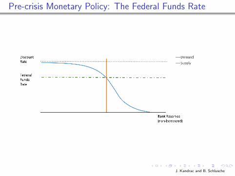
Pre-crisis Monetary Policy: The Federal Funds Rate
J. Kandrac and B. Schlusche
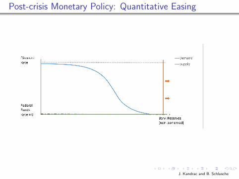
Post-crisis Monetary Policy: Quantitative Easing
J. Kandrac and B. Schlusche
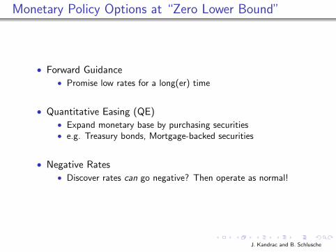
Monetary Policy Options at “Zero Lower Bound”
• Forward Guidance• Promise low rates for a long(er) time
• Quantitative Easing (QE)• Expand monetary base by purchasing securities• e.g. Treasury bonds, Mortgage-backed securities
• Negative Rates• Discover rates can go negative? Then operate as normal!
J. Kandrac and B. Schlusche
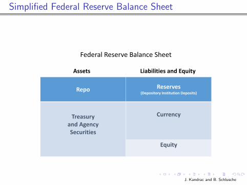
Simplified Federal Reserve Balance Sheet
Repo Reserves(Depository Institution Deposits)
Treasuryand AgencySecurities
Currency
Equity
Federal Reserve Balance Sheet
Assets Liabilities and Equity
J. Kandrac and B. Schlusche
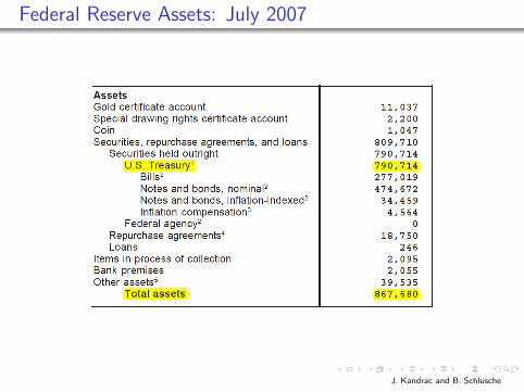
Federal Reserve Assets: July 2007
J. Kandrac and B. Schlusche
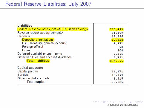
Federal Reserve Liabilities: July 2007
J. Kandrac and B. Schlusche
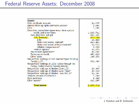
Federal Reserve Assets: December 2008
J. Kandrac and B. Schlusche
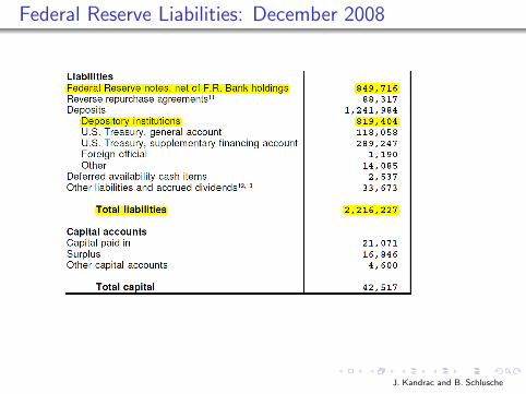
Federal Reserve Liabilities: December 2008
J. Kandrac and B. Schlusche
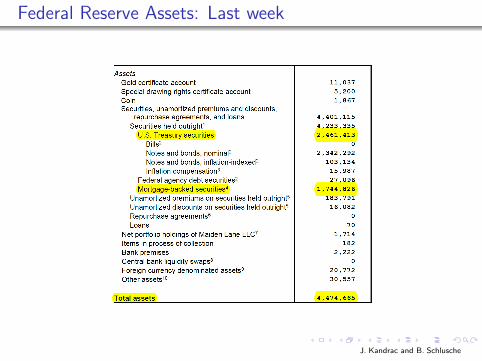
Federal Reserve Assets: Last week
J. Kandrac and B. Schlusche
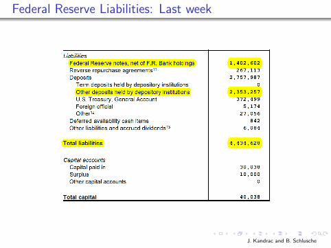
Federal Reserve Liabilities: Last week
J. Kandrac and B. Schlusche
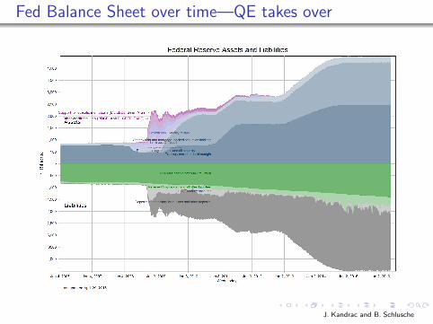
Fed Balance Sheet over time—QE takes over
J. Kandrac and B. Schlusche
How does QE help?
1. Signalling a more accommodative stance of policy
2. Portfolio Balance Channel:
• Bids up prices on purchased assets→yields fall→investors buyother assets→bids up those prices→...
J. Kandrac and B. Schlusche
Research question
• Does reserve accumulation per se contribute to thetransmission of QE?
• Banks are forced to hold the newly created reserves, inaggregate
• Why are we interested in this question?• Reserve creation is the defining characteristic of QE• Little work on the effects of forced reserve accumulation on
bank behavior or role in QE transmission• Christensen and Krogstrup (2015)
J. Kandrac and B. Schlusche
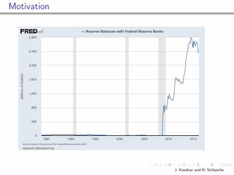
Motivation
0
400
800
1,200
1,600
2,000
2,400
2,800
1985 1990 1995 2000 2005 2010 2015
research.stlouisfed.orgSource:BoardofGovernorsoftheFederalReserveSystem(US)
ReserveBalanceswithFederalReserveBanks
(BillionsofD
ollars)
J. Kandrac and B. Schlusche
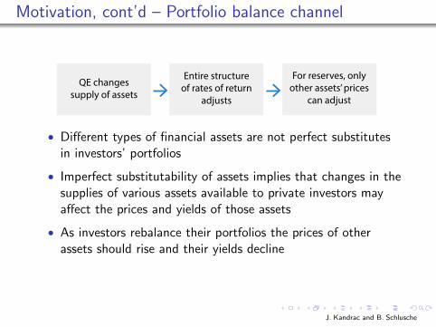
Motivation, cont’d – Portfolio balance channel
QE changes supply of assets
Entire structure of rates of return
adjusts
For reserves, only other assets’ prices
can adjust
• Different types of financial assets are not perfect substitutesin investors’ portfolios
• Imperfect substitutability of assets implies that changes in thesupplies of various assets available to private investors mayaffect the prices and yields of those assets
• As investors rebalance their portfolios the prices of otherassets should rise and their yields decline
J. Kandrac and B. Schlusche
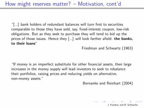
How might reserves matter? – Motivation, cont’d
“[...] bank holders of redundant balances will turn first to securitiescomparable to those they have sold, say, fixed-interest coupon, low-riskobligations. But as they seek to purchase they will tend to bid up theprices of those issues. Hence they [...] will look farther afield: the banks,to their loans”
Friedman and Schwartz (1963)
“If money is an imperfect substitute for other financial assets, then largeincreases in the money supply will lead investors to seek to rebalancetheir portfolios, raising prices and reducing yields on alternative,non-money assets.”
Bernanke and Reinhart (2004)
J. Kandrac and B. Schlusche

How to identify effects of reserves on bank-level outcomes?
• Issue: endogeneity of reserves at the bank level• Distribution of reserves across banks is determined through
private, arms-length transactions• Lending decisions can affect desired reserve holdings, or a third
factor can affect both reserve holdings AND lendingsimultaneously
• Identification strategy: instrumental variables (IV) approachexploiting a regulatory change mandated by Dodd-Frank
• Post-crisis financial reform legislation
J. Kandrac and B. Schlusche
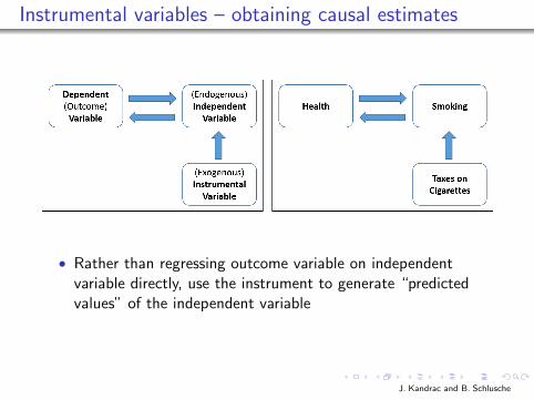
Instrumental variables – obtaining causal estimates
• Rather than regressing outcome variable on independentvariable directly, use the instrument to generate “predictedvalues” of the independent variable
J. Kandrac and B. Schlusche

Current Monetary Framework: Interest on Reserves
J. Kandrac and B. Schlusche
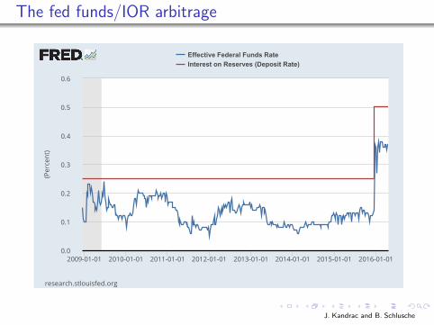
The fed funds/IOR arbitrage
0.0
0.1
0.2
0.3
0.4
0.5
0.6
2009-01-01 2010-01-01 2011-01-01 2012-01-01 2013-01-01 2014-01-01 2015-01-01 2016-01-01
research.stlouisfed.org
Effective Federal Funds RateInterest on Reserves (Deposit Rate)
(Percent)
J. Kandrac and B. Schlusche
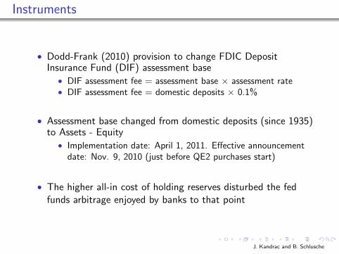
Instruments
• Dodd-Frank (2010) provision to change FDIC DepositInsurance Fund (DIF) assessment base
• DIF assessment fee = assessment base × assessment rate• DIF assessment fee = domestic deposits × 0.1%
• Assessment base changed from domestic deposits (since 1935)to Assets - Equity
• Implementation date: April 1, 2011. Effective announcementdate: Nov. 9, 2010 (just before QE2 purchases start)
• The higher all-in cost of holding reserves disturbed the fedfunds arbitrage enjoyed by banks to that point
J. Kandrac and B. Schlusche
Instruments, cont’d
• Not all banks are subject to the FDIC assessment on reserves
1. FBSEA: foreign branches and agencies established after Dec19,1991 are not covered by deposit insurance
2. Banks with custodial businesses and banker’s banks canexclude reserves from their assessment base
• For assessed institutions, the net cost of holding reserves wentup with implementation of new regulation
J. Kandrac and B. Schlusche
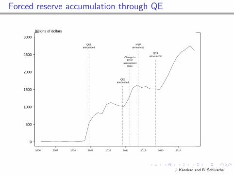
Forced reserve accumulation through QE
0
500
1000
1500
2000
2500
3000
2006 2007 2008 2009 2010 2011 2012 2013 2014
Billions of dollars
QE1announced
QE2announced
MEPannounced
Change inFDIC
assessmentbase
QE3announced
J. Kandrac and B. Schlusche
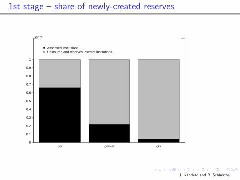
1st stage – share of newly-created reserves
QE1 QE2/MEP QE3
Share
0
0.1
0.2
0.3
0.4
0.5
0.6
0.7
0.8
0.9
1
Assessed institutionsUninsured and reserves−exempt institutions
J. Kandrac and B. Schlusche
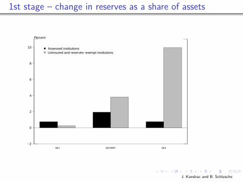
1st stage – change in reserves as a share of assets
QE1 QE2/MEP QE3
Percent
−2
0
2
4
6
8
10 Assessed institutionsUninsured and reserves−exempt institutions
J. Kandrac and B. Schlusche
Where are we?
1. Under QE, Fed forces banks to hold reserves in aggregate
2. Want to see if QE-created bank reserves cause changes inlending activity
• Problem: bank-level reserve accumulation is endogenous
3. Use a regulatory change that should affect distribution ofreserves, but did not change banks’ lending opportunities
• Showed that this regulation did predict where reserves went
J. Kandrac and B. Schlusche
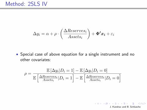
Method: 2SLS IV
∆yi = α+ ρ ·(
∆ReservesiAssetsi
)+ Φ′xi + εi
• Special case of above equation for a single instrument and noother covariates:
ρ =E [∆yi|Di = 1]− E [∆yi|Di = 0]
E[∆Reservesi
Assetsi|Di = 1
]− E
[∆Reservesi
Assetsi|Di = 0
]
J. Kandrac and B. Schlusche

Results: Total loan growth
Uninsured dummy instrument
Dependent Variable:
Total loans (percent change)QE2/MEP QE3
(1) (2) (3) (1) (2) (3)Change in Reserves 0.58*** 0.50*** 0.19 0.21*** 0.36** 0.74*
(0.08) (0.08) (0.18) (0.08) (0.17) (0.42)ln(assets) 1.45*** 2.30*** 2.30*** 3.12***
(0.52) (0.51) (0.54) (0.56)CAR 0.42** 0.86*** 0.76*** 0.62***
(0.17) (0.18) (0.21) (0.20)Lending HHI 3.11 10.9*** -6.00 -1.40
(4.51) (3.80) (5.00) (4.66)Liquidity 0.20*** 0.19*** -0.05 -0.01
(0.05) (0.04) (0.04) (0.04)Core Deposits -0.08** 0.00 0.01 0.03
(0.03) (0.03) (0.06) (0.06)
Country fixed effects — — X — — XObservations 3,135 3,135 3,135 2,859 2,859 2,859Wu-Hausman test (p-value) 0.00 0.00 0.12 0.10 0.09 0.13First-stage F -statistic 217.5 248.8 62.6 267.6 55.9 19.6
J. Kandrac and B. Schlusche
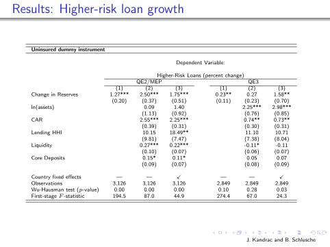
Results: Higher-risk loan growth
Uninsured dummy instrument
Dependent Variable:
Higher-Risk Loans (percent change)QE2/MEP QE3
(1) (2) (3) (1) (2) (3)Change in Reserves 1.27*** 2.50*** 1.75*** 0.23** 0.27 1.58**
(0.20) (0.37) (0.51) (0.11) (0.23) (0.70)ln(assets) 0.09 1.40 2.25*** 2.98***
(1.13) (0.92) (0.76) (0.85)CAR 2.55*** 2.25*** 0.74** 0.73**
(0.39) (0.31) (0.30) (0.31)Lending HHI 10.15 18.49** 11.10 10.71
(9.81) (7.47) (7.38) (8.04)Liquidity 0.27*** 0.22*** -0.11* -0.11
(0.10) (0.07) (0.06) (0.07)Core Deposits 0.15* 0.11* 0.05 0.07
(0.09) (0.07) (0.08) (0.09)
Country fixed effects — — X — — XObservations 3,126 3,126 3,126 2,849 2,849 2,849Wu-Hausman test (p-value) 0.00 0.00 0.00 0.10 0.28 0.03First-stage F -statistic 194.5 87.0 44.9 274.4 67.0 24.3
J. Kandrac and B. Schlusche
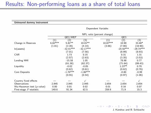
Results: Non-performing loans as a share of total loans
Uninsured dummy instrument
Dependent Variable:
NPL ratio (percent change)QE2/MEP QE3
(1) (2) (3) (1) (2) (3)Change in Reserves 6.82*** 5.81** 10.01** 10.87*** 10.90 33.48*
(1.81) (2.28) (4.14) (3.66) (7.00) (18.90)ln(assets) -32.41*** -32.17*** -24.50*** -29.74***
(7.01) (7.56) (8.99) (8.93)CAR 1.73 0.15 0.31 1.31
(2.57) (2.63) (3.35) (3.53)Lending HHI -15.58 1.05 78.98 0.77
(61.38) (62.37) (71.64) (89.43)Liquidity -0.02 -0.05 1.23** 0.70
(0.62) (0.61) (0.62) (0.76)Core Deposits -1.76*** -1.86*** -0.80 -0.99
(0.55) (0.54) (0.97) (1.06)
Country fixed effects — — X — — XObservations 2,945 2,945 2,945 2,654 2,654 2,654Wu-Hausman test (p-value) 0.00 0.01 0.02 0.01 0.16 0.07First-stage F -statistic 149.6 91.34 62.5 259.9 71.9 15.3
J. Kandrac and B. Schlusche
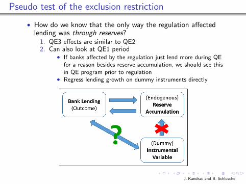
Pseudo test of the exclusion restriction
• How do we know that the only way the regulation affectedlending was through reserves?
1. QE3 effects are similar to QE22. Can also look at QE1 period
• If banks affected by the regulation just lend more during QEfor a reason besides reserve accumulation, we should see thisin QE program prior to regulation
• Regress lending growth on dummy instruments directly
J. Kandrac and B. Schlusche

Recall – share of newly-created reserves
QE1 QE2/MEP QE3
Share
0
0.1
0.2
0.3
0.4
0.5
0.6
0.7
0.8
0.9
1
Assessed institutionsUninsured and reserves−exempt institutions
J. Kandrac and B. Schlusche
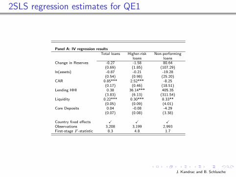
2SLS regression estimates for QE1
Panel A: IV regression resultsTotal loans Higher-risk Non-performing
loans loansChange in Reserves -0.27 -1.58 80.64
(0.69) (1.85) (107.29)ln(assets) -0.87 -0.21 -19.28
(0.54) (0.98) (25.20)CAR 0.85*** 2.52*** -8.25
(0.17) (0.46) (18.51)Lending HHI 0.38 36.14*** 405.35
(3.83) (6.13) (311.54)Liquidity 0.22*** 0.30*** 8.33**
(0.05) (0.09) (4.01)Core Deposits 0.04 -0.08 -4.29
(0.07) (0.08) (3.38)
Country fixed effects X X XObservations 3,208 3,199 2,993First-stage F -statistic 8.3 4.8 1.7
J. Kandrac and B. Schlusche
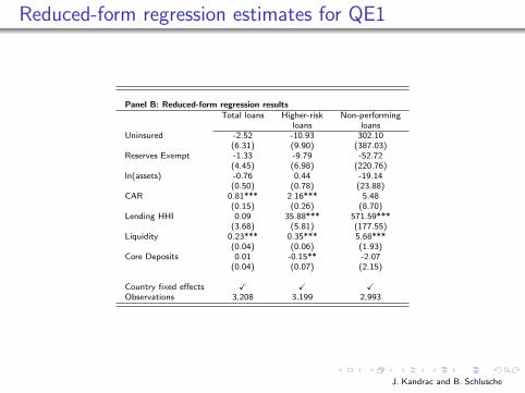
Reduced-form regression estimates for QE1
Panel B: Reduced-form regression resultsTotal loans Higher-risk Non-performing
loans loansUninsured -2.52 -10.93 302.10
(6.31) (9.90) (387.03)Reserves Exempt -1.33 -9.79 -52.72
(4.45) (6.98) (220.76)ln(assets) -0.76 0.44 -19.14
(0.50) (0.78) (23.88)CAR 0.81*** 2.16*** 5.48
(0.15) (0.26) (8.70)Lending HHI 0.09 35.88*** 571.59***
(3.68) (5.81) (177.55)Liquidity 0.23*** 0.35*** 5.68***
(0.04) (0.06) (1.93)Core Deposits 0.01 -0.15** -2.07
(0.04) (0.07) (2.15)
Country fixed effects X X XObservations 3,208 3,199 2,993
J. Kandrac and B. Schlusche
External validity
• How generalizable is our estimated LATE?
• The FDIC assessment fee altered banks’ costs of holdingreserve balances
• The ultimate holders of QE-created reserves will bedetermined by the differential costs (however defined) ofholding reserves
• The results may be more generalizable than they first appear
J. Kandrac and B. Schlusche
Conclusion
In this paper, we show the following:
• Reserve accumulation is associated with behavior consistentwith theories of portfolio substitution effects of QE
• Instrument for reserve accumulation using a regulatory changearound the time of QE2
• No first stage exists for QE1, and no evidence of an effect inreduced-form regressions for this program
• More reserves ⇒ ↑ lending growth, ↑ risk-taking
• Suggests QE works at least in part through reserveaccumulation in and of itself
Thanks!
J. Kandrac and B. Schlusche
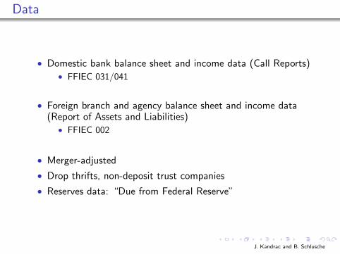
Data
• Domestic bank balance sheet and income data (Call Reports)• FFIEC 031/041
• Foreign branch and agency balance sheet and income data(Report of Assets and Liabilities)
• FFIEC 002
• Merger-adjusted
• Drop thrifts, non-deposit trust companies
• Reserves data: “Due from Federal Reserve”
J. Kandrac and B. Schlusche
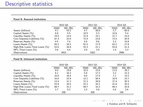
Descriptive statistics
Panel A: Assessed institutions
2010 Q4 2012 Q3 2014 Q3mean std. dev. mean std. dev. mean std. dev.
Assets (billions) 4.1 53.2 4.7 58.0 5.7 65.0Capital/Assets (%) 9.8 5.5 10.5 5.3 10.6 5.4Liquidity/Assets (%) 19.5 14.0 21.8 15.1 21.7 15.0Core Deposits/Liabilities (%) 67.3 22.0 72.4 23.8 73.5 20.9Reserves/Assets (%) 4.5 7.6 5.8 9.6 5.3 10.9Loans/Assets (%) 64.2 16.5 61.5 17.0 63.2 17.8High-Risk Loans/Total Loans (%) 53.0 20.8 52.3 21.1 52.8 21.4NPL/Total Loans (%) 3.6 4.4 2.8 3.5 1.5 2.3Observations 3453 3262 2996
Panel B: Uninsured institutions
2010 Q4 2012 Q3 2014 Q3mean std. dev. mean std. dev. mean std. dev.
Assets (billions) 9.0 19.8 10.5 23.9 13.5 28.2Capital/Assets (%) 6.1 16.3 5.8 17.2 5.2 15.3Liquidity/Assets (%) 10.0 18.4 9.0 17.5 7.1 14.2Core Deposits/Liabilities (%) 10.0 22.9 12.1 58.4 10.9 23.7Reserves/Assets (%) 13.4 21.3 21.3 26.8 27.4 30.3Loans/Assets (%) 43.9 34.5 42.2 34.2 41.8 35.5High-Risk Loans/Total Loans (%) 68.7 31.2 69.7 32.2 69.3 32.8NPL/Total Loans (%) 1.7 5.2 1.5 4.8 0.6 2.6Observations 208 200 190
J. Kandrac and B. Schlusche
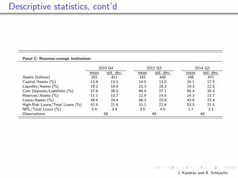
Descriptive statistics, cont’d
Panel C: Reserves-exempt institutions
2010 Q4 2012 Q3 2014 Q3mean std. dev. mean std. dev. mean std. dev.
Assets (billions) 161 411 181 440 195 471Capital/Assets (%) 13.8 13.5 14.5 13.0 16.1 17.5Liquidity/Assets (%) 19.2 18.6 21.3 18.3 19.3 12.5Core Deposits/Liabilities (%) 57.6 28.5 66.4 27.1 66.4 26.4Reserves/Assets (%) 11.1 13.7 12.9 14.6 14.3 13.7Loans/Assets (%) 49.6 24.4 46.3 23.9 43.8 23.4High-Risk Loans/Total Loans (%) 52.8 21.6 51.1 22.6 53.5 21.5NPL/Total Loans (%) 3.4 3.4 3.0 4.5 1.7 3.1Observations 50 48 48
J. Kandrac and B. Schlusche
Exclusion restriction
• Biggest concern: regulatory change affected liability side aswell
• To the extent that banks increase deposit funding, BLCdynamics might increase lending (Butt et al., 2014)
• Can rely on comparison of QE2 and QE3• QE3 started well after liability adjustments had taken place
• More generally: can’t directly test exclusion restriction but weprovide suggestive evidence of validity
• QE1 offers the opportunity to perform placebo tests• Pseudo-test of exclusion restriction when no 1st stage
J. Kandrac and B. Schlusche