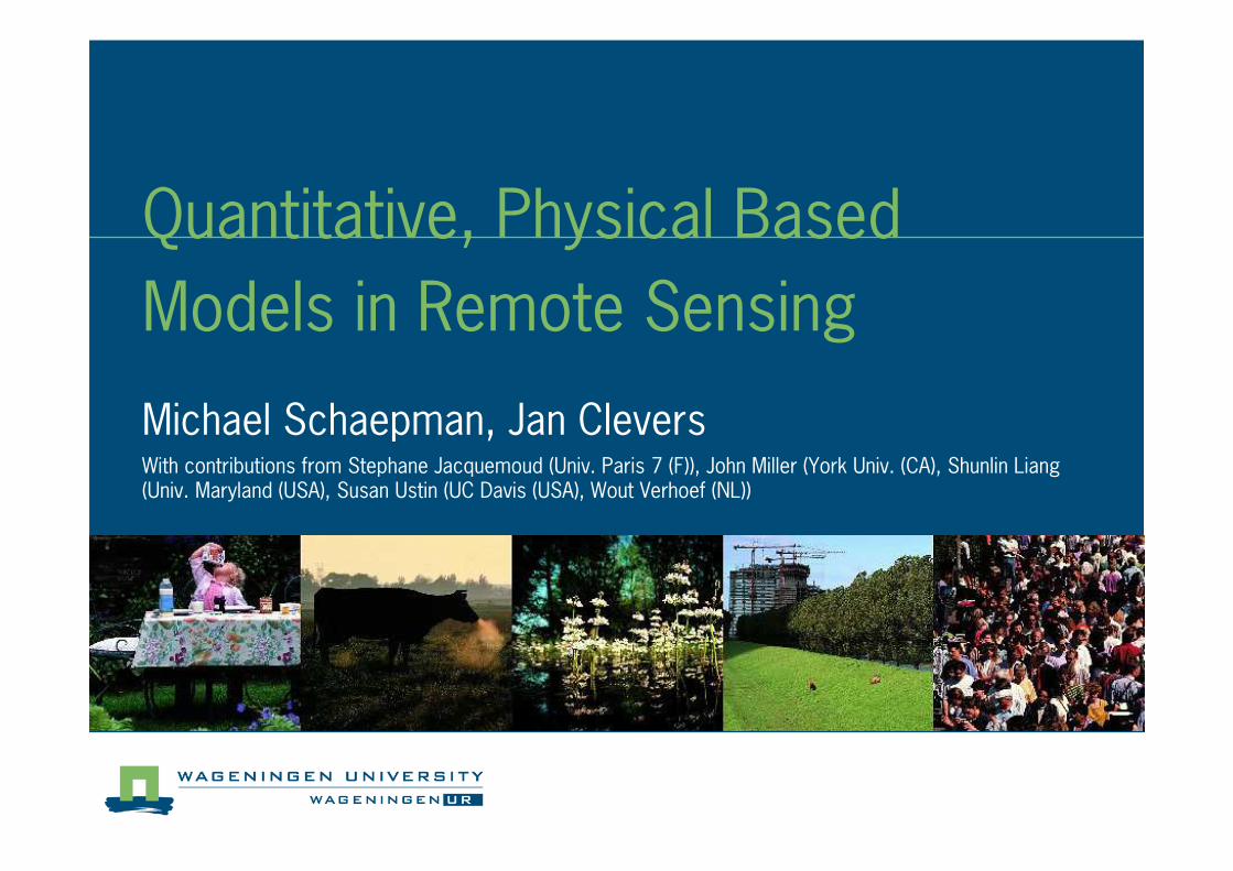
Quantitative, Physical Based

Models in Remote Sensing

Michael Schaepman, Jan CleversWith contributions from Stephane Jacquemoud (Univ. Paris 7 (F)), John Miller (York Univ. (CA), Shunlin Liang (Univ. Maryland (USA), Susan Ustin (UC Davis (USA), Wout Verhoef (NL))

Outline

� Introduction

� Challenges

� Model classes and examples

� The PROSPECT model

� The SAIL model

� Outlook

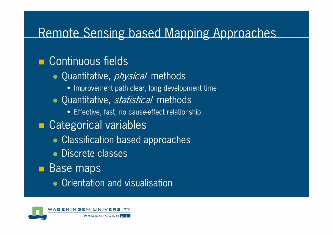
Remote Sensing based Mapping Approaches

� Continuous fields

� Quantitative, physical methods• Improvement path clear, long development time

� Quantitative, statistical methods• Effective, fast, no cause4effect relationship

� Categorical variables

� Classification based approaches

� Discrete classes

� Base maps

� Orientation and visualisation

Quantitative, physical based models

� Physical based models follow the physical laws of nature

� They establish cause4effect relationships

� If initial models do not perform well, it is usually known where to improve

� Long development and learning curve

� Complex by nature and large number of variables

Examples

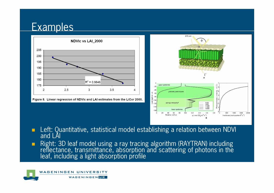
� Left: Quantitative, statistical model establishing a relation between NDVI and LAI

� Right: 3D leaf model using a ray tracing algorithm (RAYTRAN) including reflectance, transmittance, absorption and scattering of photons in the leaf, including a light absorption profile

Physical Model Challenge

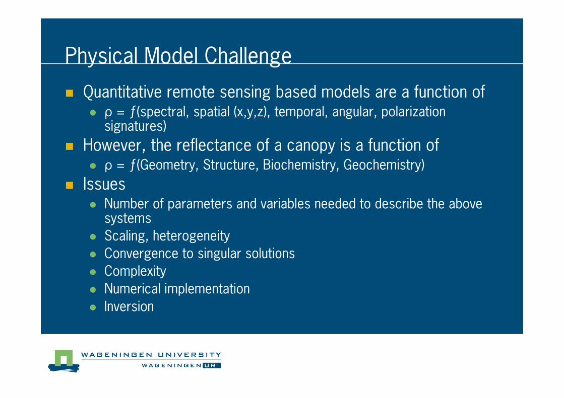
� Quantitative remote sensing based models are a function of� ρ = ƒ(spectral, spatial (x,y,z), temporal, angular, polarization

signatures)

� However, the reflectance of a canopy is a function of� ρ = ƒ(Geometry, Structure, Biochemistry, Geochemistry)

� Issues� Number of parameters and variables needed to describe the above

systems

� Scaling, heterogeneity

� Convergence to singular solutions

� Complexity

� Numerical implementation

� Inversion

Input Parameters and Variables

Fluxes considered:1. Direct solar flux2. Diffuse downward flux3. Diffuse upward flux4. Direct observed flux (radiance)

Leaf Area Index LAILIDF leaf slope parameter aLIDF bimodality parameter bHot spot parameter hotFraction brown leaf area fBLayer dissociation factor DCrown coverage CvTree shape factor zeta

Chlorophyll CabWater CwDry matter CdmSenescent material CsMesophyll structure N

Solar zenith angle szaViewing zenith angle vzaRelative azimuth angle raa

Dry soil reflectance spectrumSoil moisture SMSoil BRDF Parameters ( b, c, B0, h )

Four4stream RT modelling

Leaf/needle

Crown/canopy

Airborne

Satellite

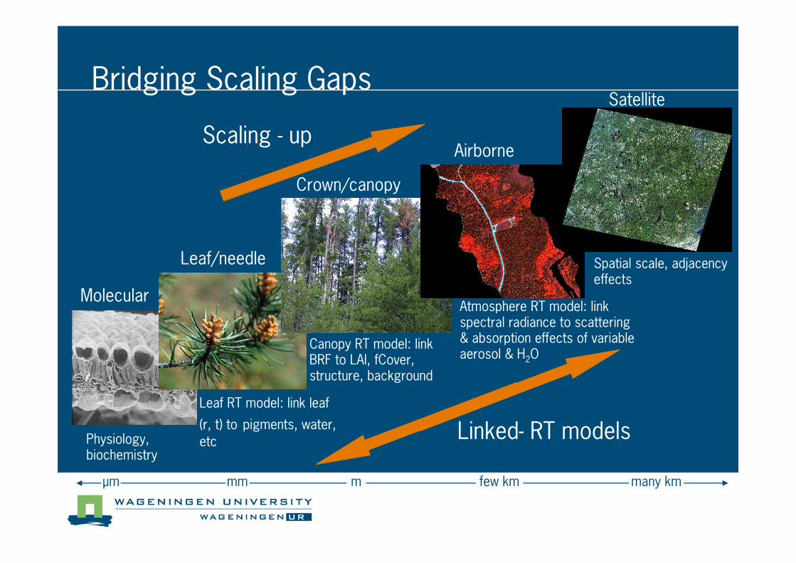
Scaling 4 up

Leaf RT model: link leaf

(r, t) to pigments, water,

etc

Canopy RT model: linkBRF to LAI, fCover, structure, background

Atmosphere RT model: linkspectral radiance to scattering& absorption effects of variable aerosol & H2O

Spatial scale, adjacencyeffects

Linked4 RT models

Bridging Scaling Gaps

Molecular

Physiology,biochemistry

Em mm m few km many km

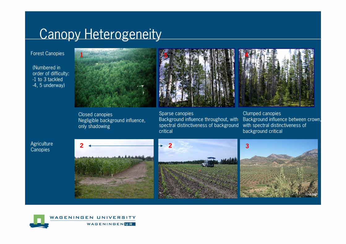
Forest Canopies

AgricultureCanopies

Closed canopiesNegligible background influence, only shadowing

Sparse canopiesBackground influence throughout, with spectral distinctiveness of background critical

Clumped canopiesBackground influence between crown,with spectral distinctiveness ofbackground critical

2

1

2 3

(Numbered in order of difficulty: 41 to 3 tackled44, 5 underway)

45

Canopy Heterogeneity

• water (vacuole): 90495%• dry matter (cell walls): 5410%

4 cellulose: 15430%4 hemicellulose: 10430%4 proteins: 10420%4 lignin: 5415%4 starch: 0.242.7%4 sugar4 etc.

• chlorophyll a and b (chloroplasts)• other pigments

4 carotenoids4 anthocyanins, flavons4 brown pigments4 etc.

B. Hosgood, S. Jacquemoud, G. Andreoli, J. Verdebout, A. Pedrini & G. Schmuck, 1994, LeafOptical Properties EXperiment 93 (LOPEX93), Joint Research Centre, Ispra, Italy.

Biochemical Leaf Composition

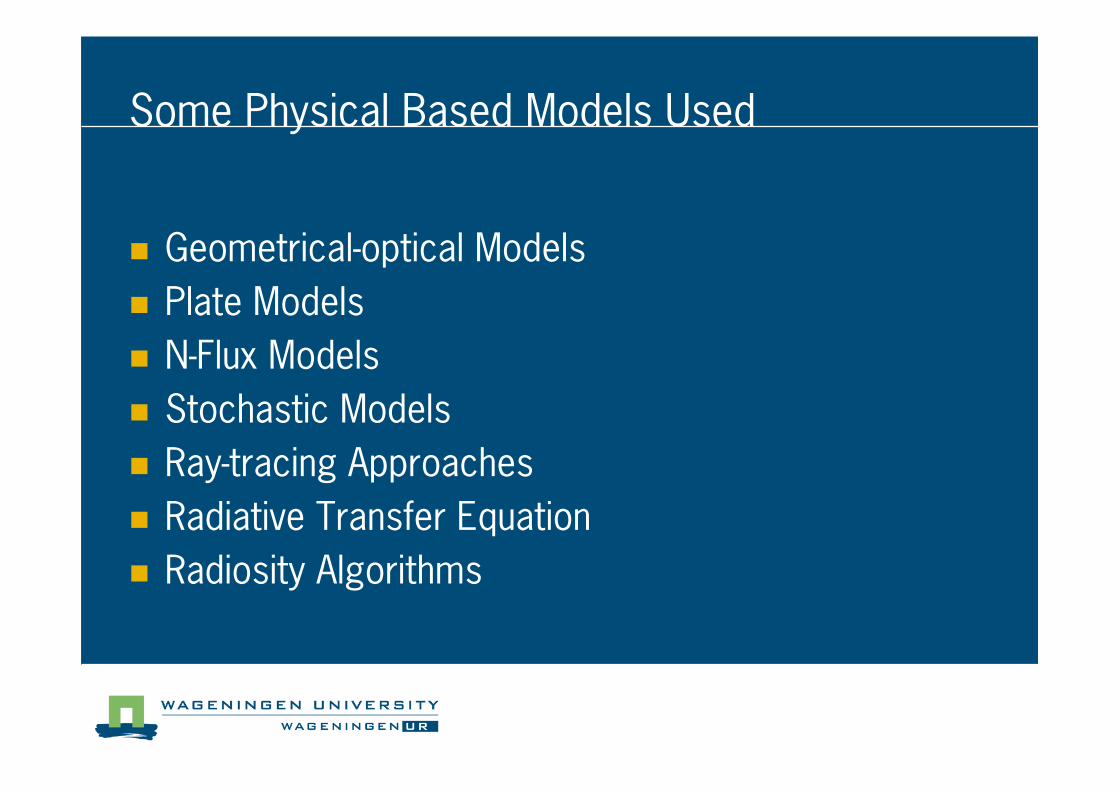
Some Physical Based Models Used

� Geometrical4optical Models

� Plate Models

� N4Flux Models

� Stochastic Models

� Ray4tracing Approaches

� Radiative Transfer Equation

� Radiosity Algorithms

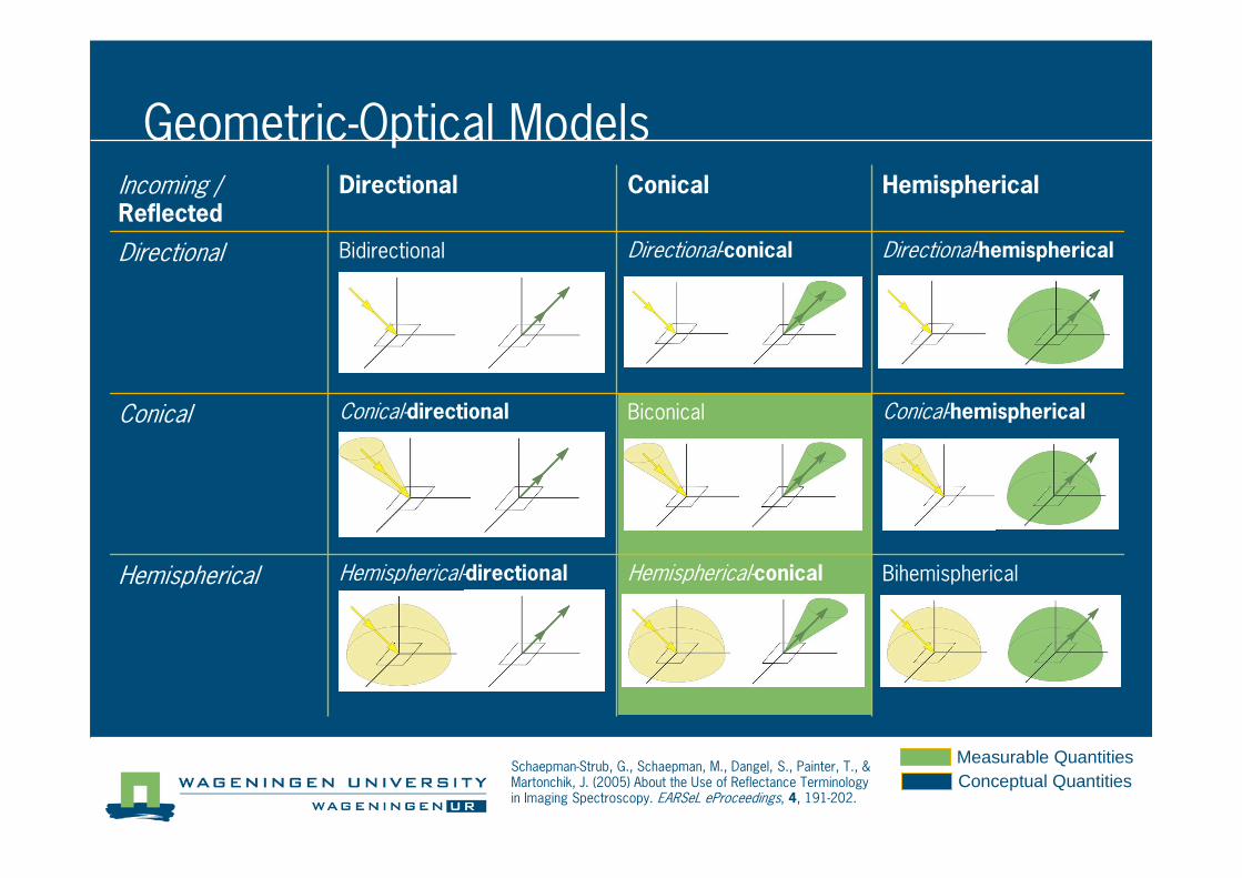
Geometric4Optical Models

BihemisphericalHemispherical4conicalHemispherical4directionalHemispherical

Conical4hemisphericalBiconicalConical4directionalConical

Directional4hemisphericalDirectional4conicalBidirectionalDirectional

HemisphericalConicalDirectionalIncoming /Reflected

Measurable QuantitiesConceptual Quantities

Schaepman4Strub, G., Schaepman, M., Dangel, S., Painter, T., & Martonchik, J. (2005) About the Use of Reflectance Terminology in Imaging Spectroscopy. EARSeL eProceedings, 4, 1914202.

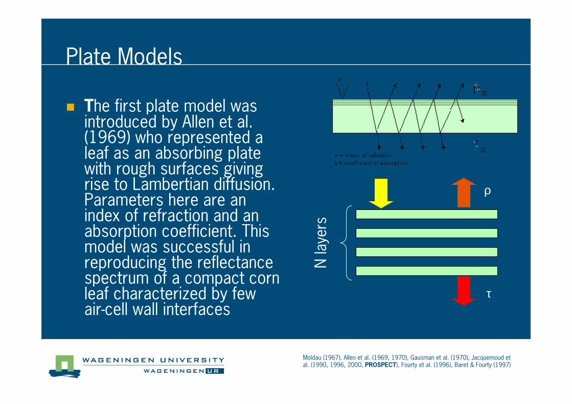
Plate Models

Moldau (1967), Allen et al. (1969, 1970), Gausman et al. (1970), Jacquemoud et al. (1990, 1996, 2000, PROSPECT), Fourty et al. (1996), Baret & Fourty (1997)

N la

yers

ρ

τ

� The first plate model was introduced by Allen et al. (1969) who represented a leaf as an absorbing plate with rough surfaces giving rise to Lambertian diffusion. Parameters here are an index of refraction and an absorption coefficient. This model was successful in reproducing the reflectance spectrum of a compact corn leaf characterized by few air4cell wall interfaces

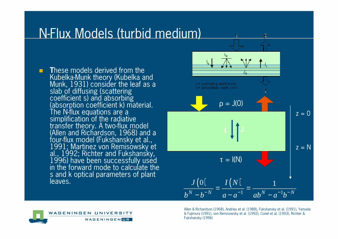
N4Flux Models (turbid medium)

� These models derived from the Kubelka4Munk theory (Kubelka and Munk, 1931) consider the leaf as a slab of diffusing (scattering coefficient s) and absorbing (absorption coefficient k) material. The N4flux equations are a simplification of the radiative transfer theory. A two4flux model (Allen and Richardson, 1968) and a four4flux model (Fukshansky et al., 1991; Martinez von Remisowsky et al., 1992; Richter and Fukshansky, 1996) have been successfully used in the forward mode to calculate the s and k optical parameters of plant leaves.

z = 0

z = N

ρ = J(0)

τ = I(N)

JI

Allen & Richardson (1968), Andrieu et al. (1988), Fukshansky et al. (1991), Yamada& Fujimura (1991), von Remisowsky et al. (1992), Conel et al. (1993), Richter & Fukshansky (1996)

( ) ( )1 1

0 1N N N N

J I N

b b a a ab a b− − − −= =− − −

Stochastic Models

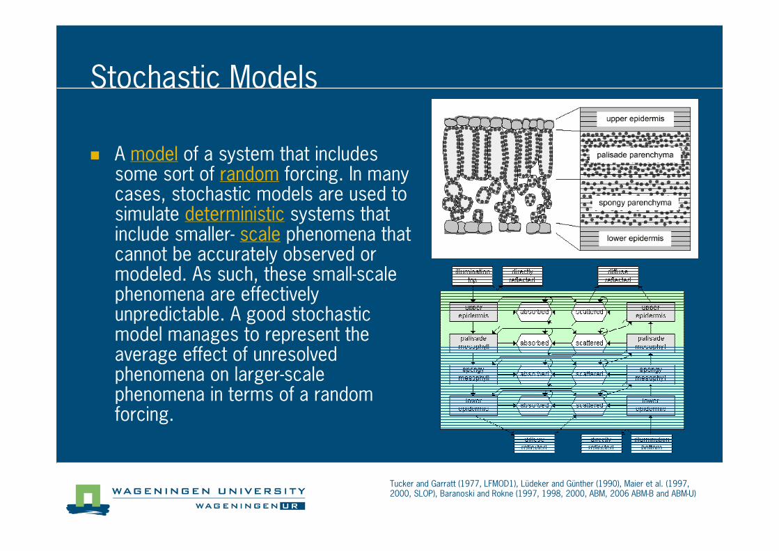
� A model of a system that includes some sort of random forcing. In many cases, stochastic models are used to simulate deterministic systems that include smaller4 scale phenomena that cannot be accurately observed or modeled. As such, these small4scale phenomena are effectively unpredictable. A good stochastic model manages to represent the average effect of unresolved phenomena on larger4scale phenomena in terms of a random forcing.

Tucker and Garratt (1977, LFMOD1), Lüdeker and Günther (1990), Maier et al. (1997, 2000, SLOP), Baranoski and Rokne (1997, 1998, 2000, ABM, 2006 ABM4B and ABM4U)

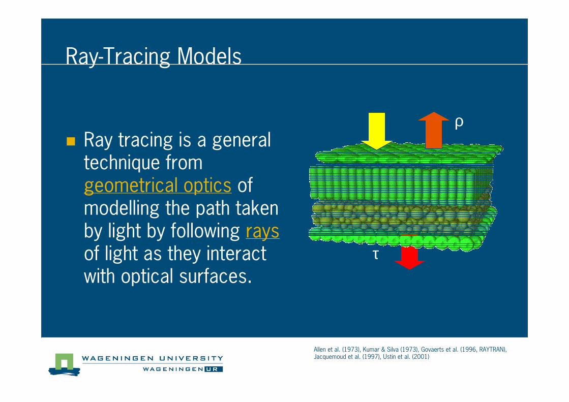
Ray4Tracing Models

� Ray tracing is a general technique from geometrical optics of modelling the path taken by light by following raysof light as they interact with optical surfaces.

ρ

τ

Allen et al. (1973), Kumar & Silva (1973), Govaerts et al. (1996, RAYTRAN), Jacquemoud et al. (1997), Ustin et al. (2001)

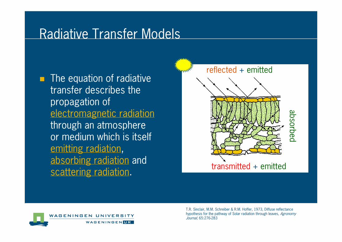
Radiative Transfer Models

� The equation of radiative transfer describes the propagation of electromagnetic radiationthrough an atmosphere or medium which is itself emitting radiation, absorbing radiation and scattering radiation.

transmitted + emitted

abso

rbed

reflected + emitted

T.R. Sinclair, M.M. Schreiber & R.M. Hoffer, 1973, Diffuse reflectancehypothesis for the pathway of Solar radiation through leaves, AgronomyJournal, 65:2764283

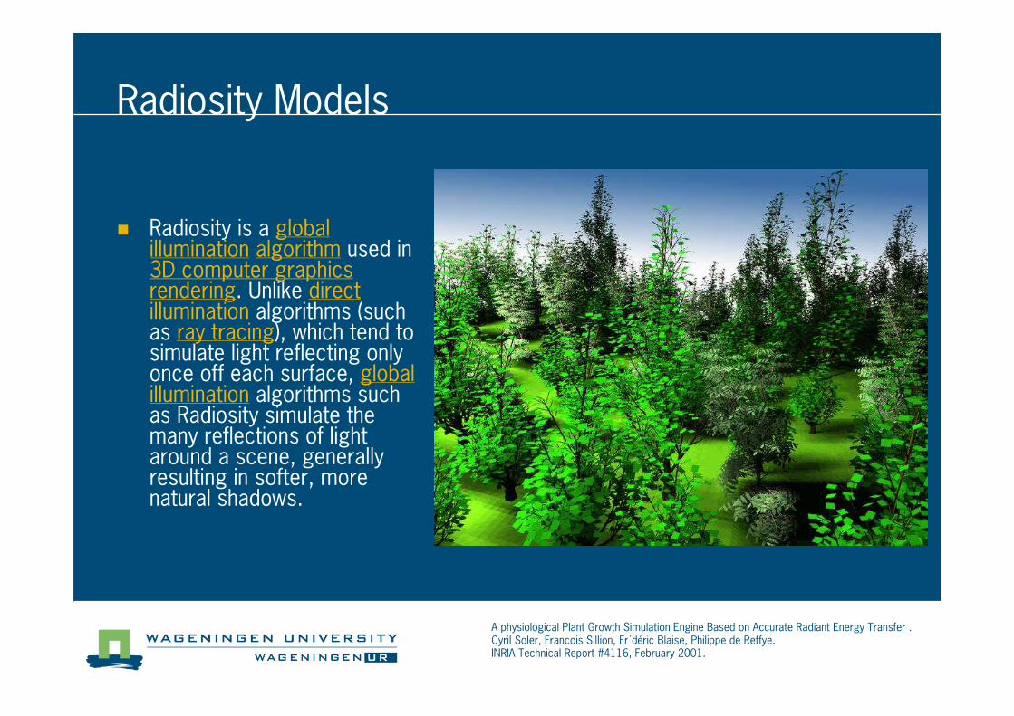
Radiosity Models

� Radiosity is a global illumination algorithm used in 3D computer graphicsrendering. Unlike direct illumination algorithms (such as ray tracing), which tend to simulate light reflecting only once off each surface, global illumination algorithms such as Radiosity simulate the many reflections of light around a scene, generally resulting in softer, more natural shadows.

A physiological Plant Growth Simulation Engine Based on Accurate Radiant Energy Transfer .Cyril Soler, Francois Sillion, Fr´déric Blaise, Philippe de Reffye. INRIA Technical Report #4116, February 2001.

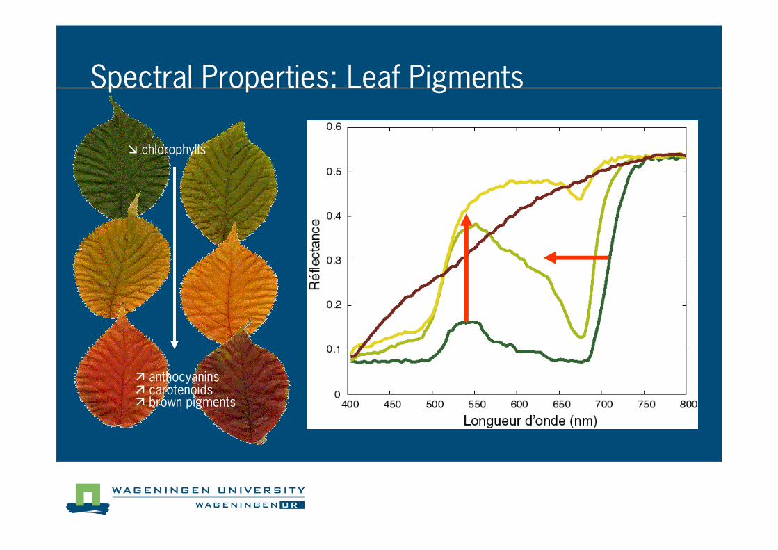
� anthocyanins� carotenoids� brown pigments

� chlorophylls

Spectral Properties: Leaf Pigments

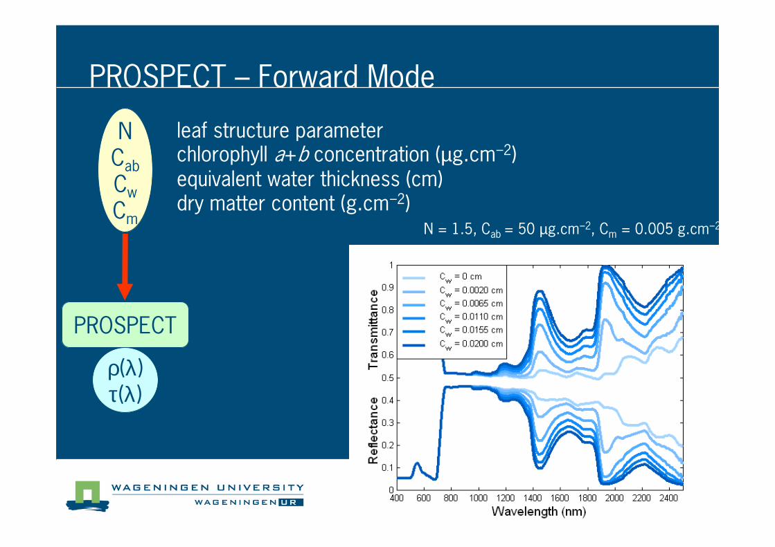
NCab

Cw

Cm

PROSPECT

ρ(λ)τ(λ)

leaf structure parameterchlorophyll a+b concentration (µg.cm−2)equivalent water thickness (cm)dry matter content (g.cm−2)

N = 1.5, Cab = 50 µg.cm−2, Cm = 0.005 g.cm−2

PROSPECT – Forward Mode

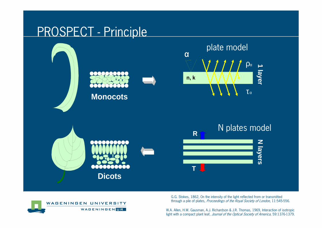
plate model

ρα

τα

αααα

n, k

N layers

T

R

1 layer

Monocots

Dicots

N plates model

W.A. Allen, H.W. Gausman, A.J. Richardson & J.R. Thomas, 1969, Interaction of isotropiclight with a compact plant leaf, Journal of the Optical Society of America, 59:137641379.

G.G. Stokes, 1862, On the intensity of the light reflected from or transmittedthrough a pile of plates, Proceedings of the Royal Society of London, 11:5454556.

PROSPECT 4 Principle

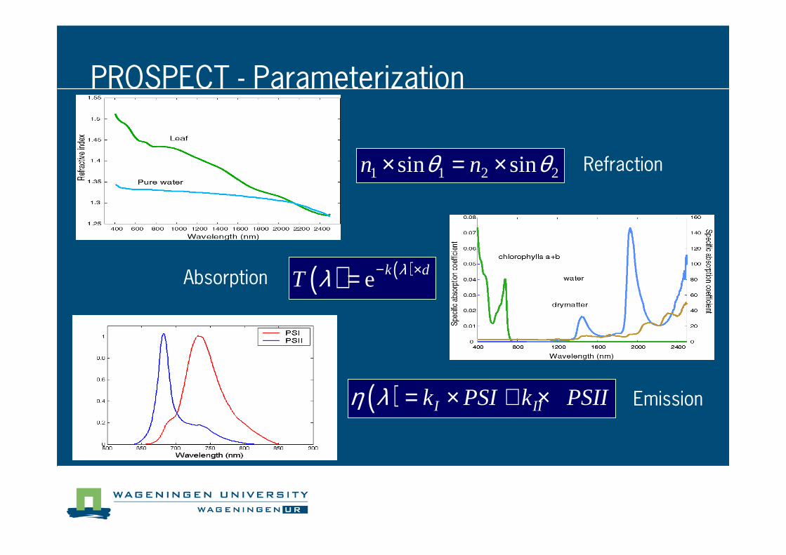
Refraction

Absorption

Emission

1 1 2 2sin sinn nθ θ× = ×

( ) ( )e k dT λλ − ×=

( ) I IIk PSI k PSIIη λ = × + ×

PROSPECT 4 Parameterization

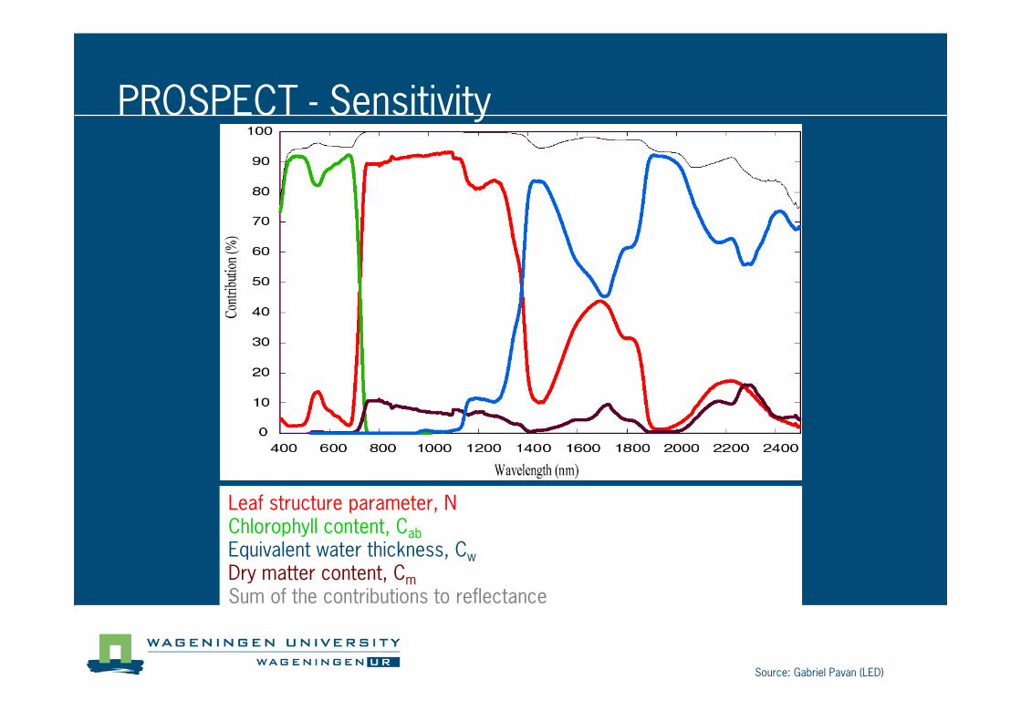
Leaf structure parameter, NChlorophyll content, Cab

Equivalent water thickness, Cw

Dry matter content, Cm

Sum of the contributions to reflectance

Source: Gabriel Pavan (LED)

PROSPECT 4 Sensitivity

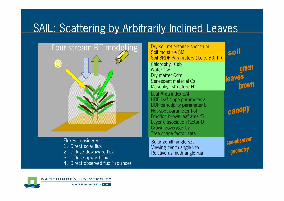
SAIL: Scattering by Arbitrarily Inclined Leaves

Fluxes considered:1. Direct solar flux2. Diffuse downward flux3. Diffuse upward flux4. Direct observed flux (radiance)

Leaf Area Index LAILIDF leaf slope parameter aLIDF bimodality parameter bHot spot parameter hotFraction brown leaf area fBLayer dissociation factor DCrown coverage CvTree shape factor zeta

Chlorophyll CabWater CwDry matter CdmSenescent material CsMesophyll structure N

Solar zenith angle szaViewing zenith angle vzaRelative azimuth angle raa

Dry soil reflectance spectrumSoil moisture SMSoil BRDF Parameters ( b, c, B0, h )

Four4stream RT modelling

SAIL: Scattering by Arbitrarily Inclined Leaves (2)

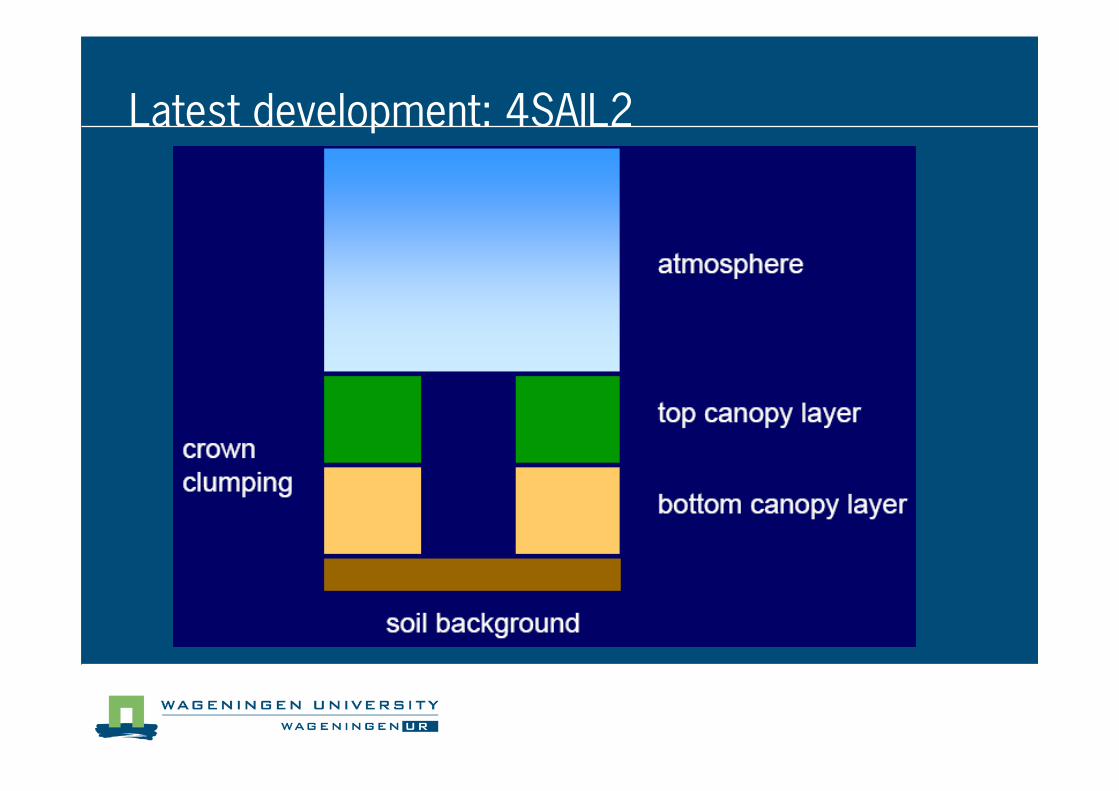
Latest development: 4SAIL2

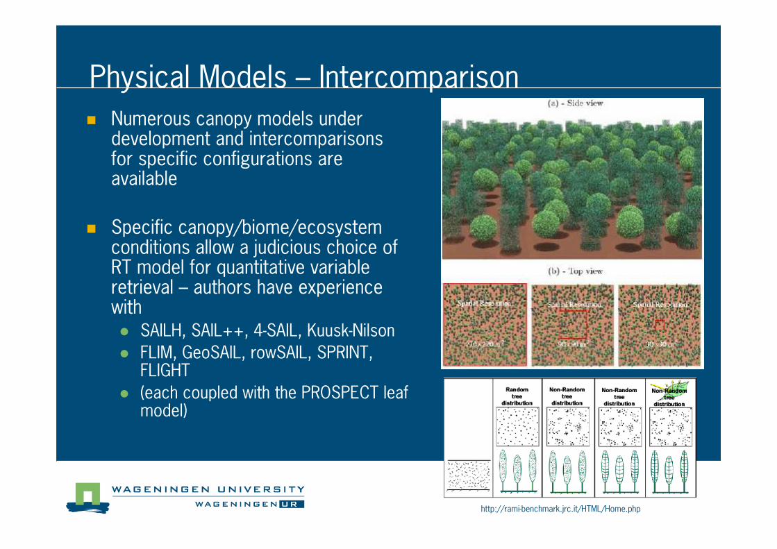
Physical Models – Intercomparison

� Numerous canopy models under development and intercomparisonsfor specific configurations are available

� Specific canopy/biome/ecosystem conditions allow a judicious choice of RT model for quantitative variable retrieval – authors have experience with� SAILH, SAIL++, 44SAIL, Kuusk4Nilson

� FLIM, GeoSAIL, rowSAIL, SPRINT, FLIGHT

� (each coupled with the PROSPECT leaf model)

http://rami4benchmark.jrc.it/HTML/Home.php

Thank you for your attention!

© Wageningen UR