quantitative relationships between modern pollen rain and ... · quantitative relationships between...

ynology 140 (2006) 61–77www.elsevier.com/locate/revpalbo

Review of Palaeobotany and Pal

Quantitative relationships between modern pollen rainand climate in the Tibetan Plateau

Caiming Shen a,b,⁎, Kam-biu Liu a, Lingyu Tang b, Jonathan T. Overpeck c

a Department of Geography and Anthropology, Louisiana State University, Baton Rouge, LA 70803, USAb Nanjing Institute of Geology and Paleontology, Academia Sinica, 39 East Beijing Road, Nanjing, 210008, People's Republic of China

c Institute for the Study of Planet Earth and Department of Geosciences, University of Arizona, Tucson, AZ 88721, USA

Received 22 July 2004; received in revised form 2 March 2006; accepted 2 March 2006Available online 19 April 2006

Abstract

Quantitative relationships between modern pollen rain and climate are poorly studied in China, partly due to the extensivehuman impact on the modern vegetation. A dataset consisting of 227 modern pollen samples from forests, shrublands, meadows,steppes, and deserts in the Tibetan Plateau, the least anthropologically-disturbed region in China, provides a unique opportunity tostudy the quantitative relationships between modern pollen rain and climate. Pollen percentage data were calculated on a sum of 20pollen taxa. Climatic data for each site, including mean annual precipitation (MAP), mean annual temperature (MAT), Julytemperature (Tjuly), and January temperature (Tjan), were derived from 214 meteorological stations in the Tibetan Plateau andadjacent areas using natural neighbor interpolation and linear interpolation methods.

Canonical correspondence analysis (CCA) was used to reveal the climatic parameters that best reflect the main patterns ofvariation in the modern pollen rain, and to detect anomalous observations. Results of CCA indicate that MAP and Tjuly are twoclimatic parameters controlling the variation of modern pollen rain in the Tibetan Plateau. Pollen–climate transfer functions forMAP and Tjuly were then developed using the inverse linear regression and weighted-averaging partial least squares regressionmodels. The functions derived from these two models are statistically significant at the 0.0000 level. A case study, in which thesefunctions were applied to a fossil pollen record from an alpine lake in the eastern Tibetan Plateau, was conducted to show thefeasibility of these functions in paleoclimate reconstruction. The results demonstrated the applicability of these pollen–climatetransfer functions to fossil pollen data.© 2006 Elsevier B.V. All rights reserved.

Keywords: modern pollen data; numerical analysis; paleoclimatic reconstruction; transfer function; palynology; Tibetan Plateau

⁎ Corresponding author. Current address: Atmospheric SciencesResearch Center, State University of New York, Albany, NY 12203,USA. Tel.: +1 518 437 8644; fax: +1 518 372 8325.

E-mail addresses: [email protected] (C. Shen),[email protected] (K. Liu).

0034-6667/$ - see front matter © 2006 Elsevier B.V. All rights reserved.doi:10.1016/j.revpalbo.2006.03.001

1. Introduction

Climate modeling provides a key to predicting futureclimates and to understanding the mechanisms of pastclimate changes. The use of climate models requires thatthe models be thoroughly tested in order to build con-fidence in their results and to identify the areas forimprovement (Webb et al., 1998). Paleoclimate data,especially quantitative data, are vital for checking the

mailto:[email protected]

mailto:[email protected]

http://dx.doi.org/10.1016/j.revpalbo.2006.03.001

62 C. Shen et al. / Review of Palaeobotany and Palynology 140 (2006) 61–77

model results. Pollen data can be calibrated in climateterms, and quantitatively reconstructed paleoclimatedata are thus needed to test model results (Huntley andPrentice, 1988, 1993; Webb et al., 1993a,b, 1998). Inthis procedure, understanding the quantitative relation-ships between modern pollen rain and contemporaryclimate is vital for estimating paleoclimatic conditionsbased on fossil pollen data (Webb and Bryson, 1972;Webb and Clark, 1977; Overpeck et al., 1985; Birks andGordon, 1985; Bartlein et al., 1986; Guiot, 1987; Birks,1995). Quantitative relationships between modern pol-len rain and climate are poorly studied in China (Shenand Tang, 1992; Song et al., 1997; Wang et al., 1997),partly due to the extensive human impact on the modernvegetation (Liu, 1988; Liu and Qiu, 1994). Modernpollen samples from the Tibetan Plateau, the least an-thropologically-disturbed region in China, provide aunique opportunity to study the quantitative relation-ships between modern pollen rain and climate.

The proven and well-established methods involvedin the quantitative reconstructions of climate includetransfer functions (Webb and Bryson, 1972; Birks,1995), response surfaces (Bartlein et al., 1986; Webb etal., 1993a,b; Markgraf et al., 2002), and the best modernanalogues (Overpeck et al., 1985; Guiot, 1987, 1990).Among these approaches, response surfaces and the best

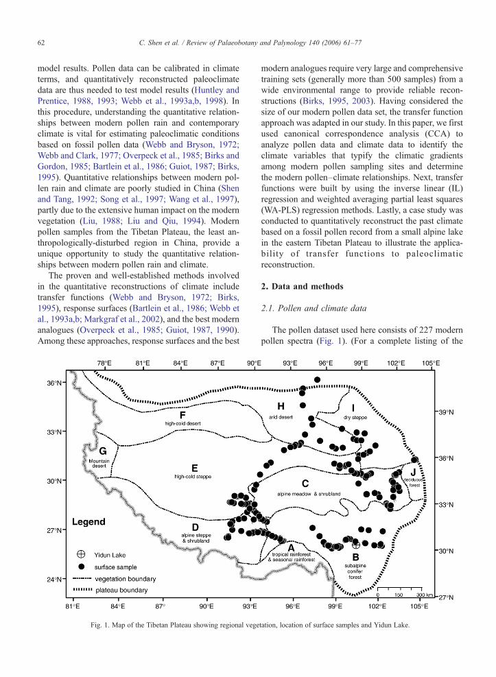
Fig. 1. Map of the Tibetan Plateau showing regional vege

modern analogues require very large and comprehensivetraining sets (generally more than 500 samples) from awide environmental range to provide reliable recon-structions (Birks, 1995, 2003). Having considered thesize of our modern pollen data set, the transfer functionapproach was adapted in our study. In this paper, we firstused canonical correspondence analysis (CCA) toanalyze pollen data and climate data to identify theclimate variables that typify the climatic gradientsamong modern pollen sampling sites and determinethe modern pollen–climate relationships. Next, transferfunctions were built by using the inverse linear (IL)regression and weighted averaging partial least squares(WA-PLS) regression methods. Lastly, a case study wasconducted to quantitatively reconstruct the past climatebased on a fossil pollen record from a small alpine lakein the eastern Tibetan Plateau to illustrate the applica-bility of transfer functions to paleoclimaticreconstruction.

2. Data and methods

2.1. Pollen and climate data

The pollen dataset used here consists of 227 modernpollen spectra (Fig. 1). (For a complete listing of the

tation, location of surface samples and Yidun Lake.

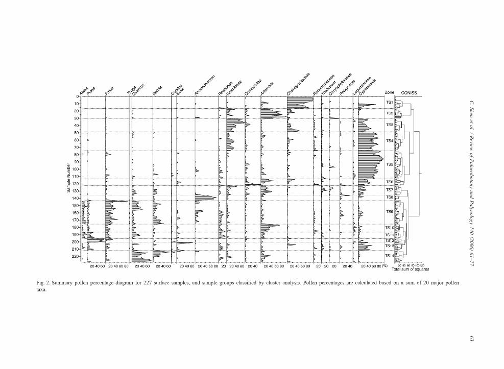
Fig. 2. Summary pollen percentage diagram for 227 surface samples, and sample groups classified by cluster analysis. Pollen percentages are calculated based on a sum of 20 major pollentaxa.

63C.Shen

etal.

/Review

ofPalaeobotany

andPalynology

140(2006)

61–77


modern pollen dataset, see Shen, 2003) For datastandardization and consistency, 20 pollen types wereselected to represent the major and minor pollen types inthe modern pollen spectra. New pollen percentages wererecalculated based on a sum of these 20 pollen types(Fig. 2). Among these 20 pollen types, major tree pollentypes are Abies, Picea, Pinus, Quercus, and Betula;shrub pollen types are Rhododendron, Rosaceae, andSalix; and herb pollen types are Gramineae, Composi-tae, Artemisia, Chenopodiaceae, and Cyperaceae. Minorpollen types include tree pollen Tsuga and Corylus, andherb taxa Ranunculaceae, Thalictrum, Caryophyllaceae,Polygonum, and Leguminosae. Cupressaceae pollen wasexcluded from the major pollen types because it is poorlypreserved in fossil pollen spectra (Shen, 2003).

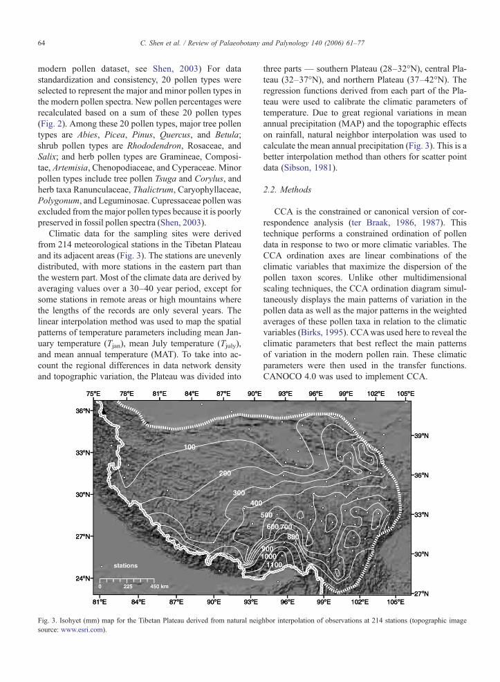
Climatic data for the sampling sites were derivedfrom 214 meteorological stations in the Tibetan Plateauand its adjacent areas (Fig. 3). The stations are unevenlydistributed, with more stations in the eastern part thanthe western part. Most of the climate data are derived byaveraging values over a 30–40 year period, except forsome stations in remote areas or high mountains wherethe lengths of the records are only several years. Thelinear interpolation method was used to map the spatialpatterns of temperature parameters including mean Jan-uary temperature (Tjan), mean July temperature (Tjuly),and mean annual temperature (MAT). To take into ac-count the regional differences in data network densityand topographic variation, the Plateau was divided into

Fig. 3. Isohyet (mm) map for the Tibetan Plateau derived from natural neigsource: www.esri.com).

three parts — southern Plateau (28–32°N), central Pla-teau (32–37°N), and northern Plateau (37–42°N). Theregression functions derived from each part of the Pla-teau were used to calibrate the climatic parameters oftemperature. Due to great regional variations in meanannual precipitation (MAP) and the topographic effectson rainfall, natural neighbor interpolation was used tocalculate the mean annual precipitation (Fig. 3). This is abetter interpolation method than others for scatter pointdata (Sibson, 1981).

2.2. Methods

CCA is the constrained or canonical version of cor-respondence analysis (ter Braak, 1986, 1987). Thistechnique performs a constrained ordination of pollendata in response to two or more climatic variables. TheCCA ordination axes are linear combinations of theclimatic variables that maximize the dispersion of thepollen taxon scores. Unlike other multidimensionalscaling techniques, the CCA ordination diagram simul-taneously displays the main patterns of variation in thepollen data as well as the major patterns in the weightedaverages of these pollen taxa in relation to the climaticvariables (Birks, 1995). CCAwas used here to reveal theclimatic parameters that best reflect the main patternsof variation in the modern pollen rain. These climaticparameters were then used in the transfer functions.CANOCO 4.0 was used to implement CCA.

hbor interpolation of observations at 214 stations (topographic image

http://www.esri.com

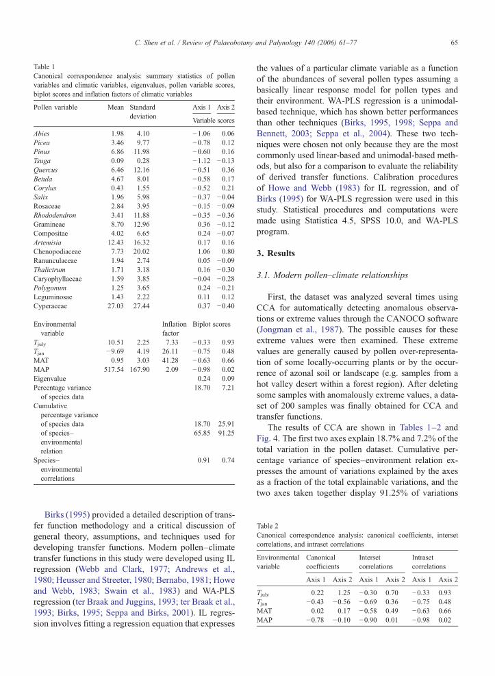
Table 1Canonical correspondence analysis: summary statistics of pollenvariables and climatic variables, eigenvalues, pollen variable scores,biplot scores and inflation factors of climatic variables

Pollen variable Mean Standarddeviation

Axis 1 Axis 2

Variable scores

Abies 1.98 4.10 −1.06 0.06Picea 3.46 9.77 −0.78 0.12Pinus 6.86 11.98 −0.60 0.16Tsuga 0.09 0.28 −1.12 −0.13Quercus 6.46 12.16 −0.51 0.36Betula 4.67 8.01 −0.58 0.17Corylus 0.43 1.55 −0.52 0.21Salix 1.96 5.98 −0.37 −0.04Rosaceae 2.84 3.95 −0.15 −0.09Rhododendron 3.41 11.88 −0.35 −0.36Gramineae 8.70 12.96 0.36 −0.12Compositae 4.02 6.65 0.24 −0.07Artemisia 12.43 16.32 0.17 0.16Chenopodiaceae 7.73 20.02 1.06 0.80Ranunculaceae 1.94 2.74 0.05 −0.09Thalictrum 1.71 3.18 0.16 −0.30Caryophyllaceae 1.59 3.85 −0.04 −0.28Polygonum 1.25 3.65 0.24 −0.21Leguminosae 1.43 2.22 0.11 0.12Cyperaceae 27.03 27.44 0.37 −0.40

Environmentalvariable

Inflationfactor

Biplot scores

Tjuly 10.51 2.25 7.33 −0.33 0.93Tjan −9.69 4.19 26.11 −0.75 0.48MAT 0.95 3.03 41.28 −0.63 0.66MAP 517.54 167.90 2.09 −0.98 0.02Eigenvalue 0.24 0.09Percentage variance

of species data18.70 7.21

Cumulativepercentage varianceof species data 18.70 25.91of species–environmentalrelation

65.85 91.25

Species–environmentalcorrelations

0.91 0.74

Table 2Canonical correspondence analysis: canonical coefficients, intersetcorrelations, and intraset correlations

Environmentalvariable

Canonicalcoefficients

Intersetcorrelations

Intrasetcorrelations

Axis 1 Axis 2 Axis 1 Axis 2 Axis 1 Axis 2

Tjuly 0.22 1.25 −0.30 0.70 −0.33 0.93Tjan −0.43 −0.56 −0.69 0.36 −0.75 0.48MAT 0.02 0.17 −0.58 0.49 −0.63 0.66MAP −0.78 −0.10 −0.90 0.01 −0.98 0.02

65C. Shen et al. / Review of Palaeobotany and Palynology 140 (2006) 61–77

Birks (1995) provided a detailed description of trans-fer function methodology and a critical discussion ofgeneral theory, assumptions, and techniques used fordeveloping transfer functions. Modern pollen–climatetransfer functions in this study were developed using ILregression (Webb and Clark, 1977; Andrews et al.,1980; Heusser and Streeter, 1980; Bernabo, 1981; Howeand Webb, 1983; Swain et al., 1983) and WA-PLSregression (ter Braak and Juggins, 1993; ter Braak et al.,1993; Birks, 1995; Seppa and Birks, 2001). IL regres-sion involves fitting a regression equation that expresses

the values of a particular climate variable as a functionof the abundances of several pollen types assuming abasically linear response model for pollen types andtheir environment. WA-PLS regression is a unimodal-based technique, which has shown better performancesthan other techniques (Birks, 1995, 1998; Seppa andBennett, 2003; Seppa et al., 2004). These two tech-niques were chosen not only because they are the mostcommonly used linear-based and unimodal-based meth-ods, but also for a comparison to evaluate the reliabilityof derived transfer functions. Calibration proceduresof Howe and Webb (1983) for IL regression, and ofBirks (1995) for WA-PLS regression were used in thisstudy. Statistical procedures and computations weremade using Statistica 4.5, SPSS 10.0, and WA-PLSprogram.

3. Results

3.1. Modern pollen–climate relationships

First, the dataset was analyzed several times usingCCA for automatically detecting anomalous observa-tions or extreme values through the CANOCO software(Jongman et al., 1987). The possible causes for theseextreme values were then examined. These extremevalues are generally caused by pollen over-representa-tion of some locally-occurring plants or by the occur-rence of azonal soil or landscape (e.g. samples from ahot valley desert within a forest region). After deletingsome samples with anomalously extreme values, a data-set of 200 samples was finally obtained for CCA andtransfer functions.

The results of CCA are shown in Tables 1–2 andFig. 4. The first two axes explain 18.7% and 7.2% of thetotal variation in the pollen dataset. Cumulative per-centage variance of species–environment relation ex-presses the amount of variations explained by the axesas a fraction of the total explainable variations, and thetwo axes taken together display 91.25% of variations

s

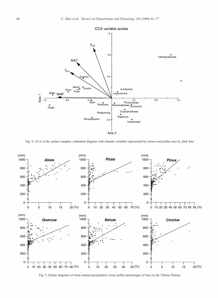
Fig. 4. CCA of the surface samples: ordination diagram with climatic variables represented by arrows and pollen taxa by dark dots.

Fig. 5. Scatter diagrams of mean annual precipitation versus pollen percentages of trees in the Tibetan Plateau.


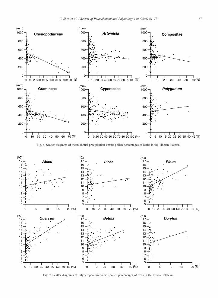
Fig. 6. Scatter diagrams of mean annual precipitation versus pollen percentages of herbs in the Tibetan Plateau.

Fig. 7. Scatter diagrams of July temperature versus pollen percentages of trees in the Tibetan Plateau.



that can be explained by the variables. The first eigen-value is fairly high, implying that the first axis representsa fairly strong gradient. CCA axis 1 accounts for 65.85%of the species–environment relation. The species–envi-ronment correlations indicate how much of the variationin the pollen data on one CCA axis is explained by theenvironmental variables. The large figure of 0.91 sug-gests that the climatic variables can account for most ofthe variation in the pollen data on CCA axis 1. In Fig. 4,the lengths and positions of the arrows depend on theeigenvalues and on the intraset correlations (Table 2).They provide information about the relationship betweenthe climatic variables and the derived axes (Jongmanet al., 1987). Arrows that are parallel to an axis indi-cate a correlation. The length of the arrow reflects thestrength of that correlation. Climatic variables withlong arrows are more strongly correlated with the or-dination axes than those with short arrows. Thus,MAP ismost strongly related to axis 1 and least to axis 2,whereas Tjuly is inversely related to MAP. Tjan and MATare not highly related to either axis 1 or axis 2. On theother hand, inflation factors also indicate that Tjan andMAT are not as important as MAP and Tjuly. A largeinflation factor implies that the variable is redundant withother variables in the dataset. It is not surprising sinceMAT is highly correlated with Tjuly and all temperatures

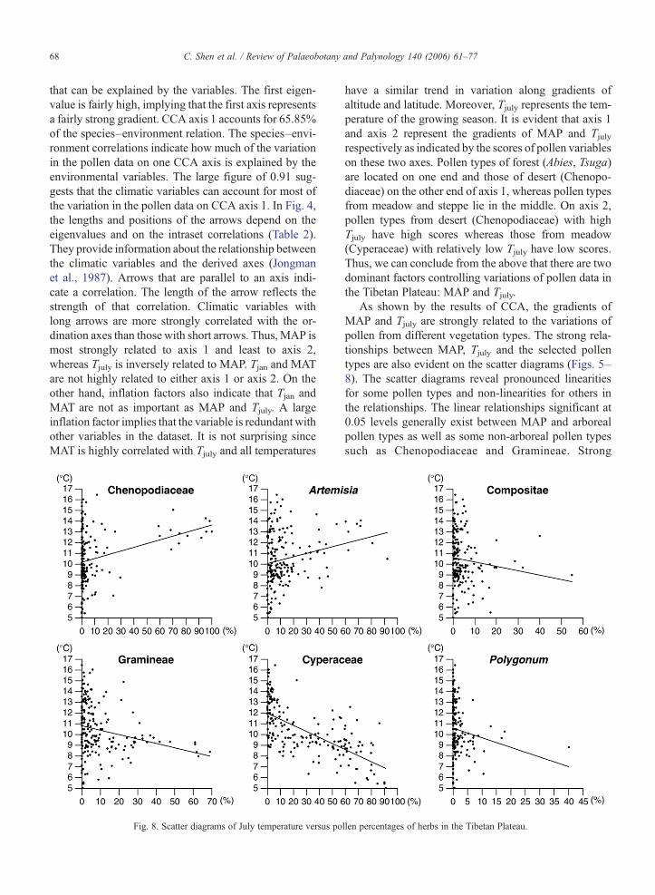
Fig. 8. Scatter diagrams of July temperature versus po

have a similar trend in variation along gradients ofaltitude and latitude. Moreover, Tjuly represents the tem-perature of the growing season. It is evident that axis 1and axis 2 represent the gradients of MAP and Tjulyrespectively as indicated by the scores of pollen variableson these two axes. Pollen types of forest (Abies, Tsuga)are located on one end and those of desert (Chenopo-diaceae) on the other end of axis 1, whereas pollen typesfrom meadow and steppe lie in the middle. On axis 2,pollen types from desert (Chenopodiaceae) with highTjuly have high scores whereas those from meadow(Cyperaceae) with relatively low Tjuly have low scores.Thus, we can conclude from the above that there are twodominant factors controlling variations of pollen data inthe Tibetan Plateau: MAP and Tjuly.

As shown by the results of CCA, the gradients ofMAP and Tjuly are strongly related to the variations ofpollen from different vegetation types. The strong rela-tionships between MAP, Tjuly and the selected pollentypes are also evident on the scatter diagrams (Figs. 5–8). The scatter diagrams reveal pronounced linearitiesfor some pollen types and non-linearities for others inthe relationships. The linear relationships significant at0.05 levels generally exist between MAP and arborealpollen types as well as some non-arboreal pollen typessuch as Chenopodiaceae and Gramineae. Strong

llen percentages of herbs in the Tibetan Plateau.


positive correlations are found between Tjuly and treepollen types such as Pinus, Quercus, Betula, and weakpositive relationships between Tjuly, Chenopodiaceaeand Artemisia. Markedly negative correlations occurbetween Tjuly and Cyperaceae.

3.2. Transfer functions

The forward stepwise method was used in the ILregression analysis. The performance of the IL regres-sion is reported in Table 3 and Fig. 9. The MAP equa-

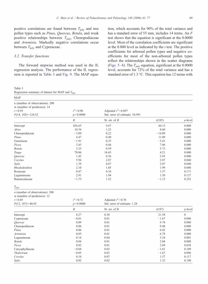
Table 3Regression summary of dataset for MAP and Tjuly

MAP

n (number of observations): 200m (number of predictors): 14r=0.95 r2=0.90 AdF(14, 185)=124.52 pb0.0000 St

B St

Intercept 426.65 9Abies 10.54 1Chenopodiaceae −3.09 0Pinus 4.47 0Gramineae −1.91 0Picea 3.43 0Betula 3.35 0Tsuga 70.06 16Quercus 1.42 0Corylus 5.94 2Salix 1.39 0Rhododendron 2.10 1Rosaceae 0.47 0Leguminosae 2.91 1Ranunculaceae −1.75 1

Tjuly

n (number of observations): 200m (number of predictors): 12r=0.85 r2=0.72 AdF(12, 187)=40.05 pb0.0000 St

B St

Intercept 8.27 0.3Cyperaceae −0.01 0.0Quercus 0.09 0.0Chenopodiaceae 0.06 0.0Pinus 0.06 0.0Artemisia 0.05 0.0Leguminosae 0.14 0.0Betula 0.04 0.0Picea 0.02 0.0Caryophyllaceae −0.04 0.0Thalictrum −0.05 0.0Corylus 0.10 0.0Salix 0.02 0.0

tion, which accounts for 90% of the total variance andhas a standard error of 55 mm, includes 14 terms. An Ftest shows that the equation is significant at the 0.0000level. Most of the correlation coefficients are significantat the 0.000 level as indicated by the t test. The positivecoefficients for arboreal pollen types and negative co-efficients for most of the non-arboreal pollen typesreflect the relationships shown in the scatter diagrams(Figs. 5–8). The Tjuly equation, significant at the 0.0000level, accounts for 72% of the total variance and has astandard error of 1.3 °C. This equation has 12 terms with

justed r2=0.897d. error of estimate: 54.991

. err. of B t(185) p-level

.67 44.12 0.000

.23 8.60 0.000

.22 −14.09 0.000

.40 11.09 0.000

.35 −5.41 0.000

.44 7.86 0.000

.59 5.73 0.000

.65 4.21 0.000

.36 3.93 0.000

.87 2.07 0.040

.67 2.07 0.040

.05 1.99 0.048

.34 1.37 0.171

.94 1.50 0.137

.52 −1.15 0.252

justed r2=0.70d. error of estimate: 1.28

. err. of B t(187) p-level

8 21.58 01 −1.67 0.0961 9.78 0.0001 9.48 0.0001 6.82 0.0001 6.78 0.0004 3.24 0.0011 2.68 0.0081 2.09 0.0383 −1.61 0.1093 −1.67 0.0967 1.57 0.1172 1.32 0.190

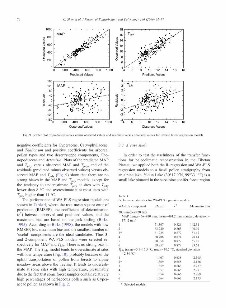
Fig. 9. Scatter plot of predicted values versus observed values and residuals versus observed values for inverse linear regression models.

Table 4Performance statistics for WA-PLS regression models

WA-PLS component RMSEP r2 Maximum bias

200 samples×20 taxaMAP (range=66–910 mm, mean=494.2 mm, standard deviation=171.2 mm)

1 71.307 0.826 142.312 63.220 0.863 100.993⁎ 61.225 0.872 81.474 60.706 0.874 78.145 60.058 0.877 65.856 59.857 0.877 73.61Tjuly (range=5.1–16.5 °C, mean=10.5 °C, standard deviation=2.34 °C)

1 1.407 0.638 2.5052* 1.369 0.658 2.1863 1.359 0.663 2.2374 1.357 0.665 2.2715 1.354 0.666 2.2696 1.364 0.662 2.173

* Selected models.


negative coefficients for Cyperaceae, Caryophyllaceae,and Thalictrum and positive coefficients for arborealpollen types and two desert/steppe components, Che-nopodiaceae and Artemisia. Plots of the predicted MAPand Tjuly versus observed MAP and Tjuly, and of theresiduals (predicted minus observed values) versus ob-served MAP and Tjuly (Fig. 9) show that there are nostrong biases in the MAP and Tjuly models, except forthe tendency to underestimate Tjuly at sites with Tjulylower than 8 °C and overestimate it at most sites withTjuly higher than 11 °C.

The performance of WA-PLS regression models areshown in Table 4, where the root mean square error ofprediction (RMSEP), the coefficient of determination(r2) between observed and predicted values, and themaximum bias are based on the jack-knifing (Birks,1995). According to Birks (1998), the models with lowRMSEP, low maximum bias and the smallest number of‘useful’ components are the ideal candidates. Thus 3-and 2-component WA-PLS models were selected re-spectively for MAP and Tjuly. There is no strong bias inthe MAP. The Tjuly model tends to overestimate at siteswith low temperature (Fig. 10), probably because of theuphill transportation of pollen from forests to alpinemeadow areas above the treeline. It tends to underesti-mate at some sites with high temperature, presumablydue to the fact that some forest samples contain relativelyhigh percentages of herbaceous pollen such as Cyper-aceae pollen as shown in Fig. 2.

3.3. A case study

In order to test the usefulness of the transfer func-tions for paleoclimatic reconstruction in the TibetanPlateau, we applied both the IL regression and WA-PLSregression models to a fossil pollen stratigraphy froman alpine lake. Yidun Lake (30°17.9′N, 99°33.1′E) is asmall lake situated in the subalpine conifer forest region

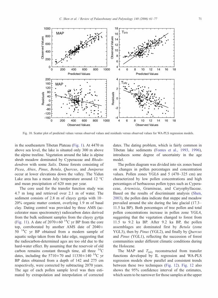
Fig. 10. Scatter plot of predicted values versus observed values and residuals versus observed values for WA-PLS regression models.


in the southeastern Tibetan Plateau (Fig. 1). At 4470 mabove sea level, the lake is situated only 300 m abovethe alpine treeline. Vegetation around the lake is alpineshrub meadow dominated by Cyperaceae and Rhodo-dendron with some Salix. Dense forests consisting ofPicea, Abies, Pinus, Betula, Quercus, and Juniperusoccur at lower elevations down the valley. The YidunLake area has a mean July temperature around 12 °Cand mean precipitation of 620 mm per year.

The core used for the transfer function study was4.7 m long and retrieved over 2.1 m of water. Thesediment consists of 2.8 m of clayey gyttja with 10–20% organic matter content, overlying 1.9 m of basalclay. Dating control was provided by three AMS (ac-celerator mass spectrometry) radiocarbon dates derivedfrom the bulk sediment samples from the clayey gyttja(Fig. 11). A date of 2070±60 14C yr BP from the coretop, corroborated by another AMS date of 2040±50 14C yr BP obtained from a modern sample ofaquatic sedge taken from the lake edge, suggesting thatthe radiocarbon-determined ages are too old due to thehard-water effect. By assuming that the reservoir of oldcarbon remains constant through time, all three 14Cdates, including the 5710±70 and 11330±140 14C yrBP dates obtained from a depth of 142 and 275 cmrespectively, were corrected by subtracting 2070 years.The age of each pollen sample level was then esti-mated by extrapolation and interpolation of corrected

dates. The dating problem, which is fairly common inTibetan lake sediments (Fontes et al., 1993, 1996),introduces some degree of uncertainty in the agemodel.

The pollen diagram was divided into six zones basedon changes in pollen percentages and concentrationvalues. Pollen zones YGL6 and 5 (470–325 cm) arecharacterized by low pollen concentrations and highpercentages of herbaceous pollen types such as Cypera-ceae, Artemisia, Gramineae, and Caryophyllaceae.Based on the results of discriminant analysis (Shen,2003), the pollen data indicate that steppe and meadowprevailed around the site during the late glacial (17.3–11.5 ka BP). Both percentages of tree pollen and totalpollen concentrations increase in pollen zone YGL4,suggesting that the vegetation changed to forest from11.5 to 9.2 ka BP. After 9.2 ka BP, the pollenassemblages are dominated first by Betula (zoneYGL3), then by Pinus (YGL2), and finally by Quercusand Pinus (YGL1), reflecting the succession of forestcommunities under different climatic conditions duringthe Holocene.

The MAP and Tjuly reconstructed from transferfunctions developed by IL regression and WA-PLSregression models show parallel and consistent trendsbetween these two techniques (Fig. 12). Fig. 12 alsoshows the 95% confidence interval of the estimates,which seem to be narrower for those samples at the upper

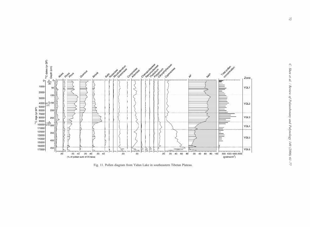
Fig. 11. Pollen diagram from Yidun Lake in southeastern Tibetan Plateau.

72C.Shen

etal.

/Review

ofPalaeobotany

andPalynology

140(2006)

61–77

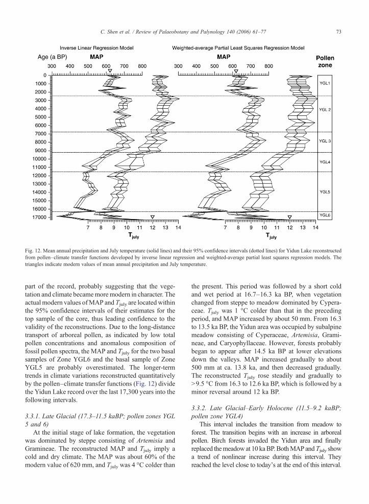
Fig. 12. Mean annual precipitation and July temperature (solid lines) and their 95% confidence intervals (dotted lines) for Yidun Lake reconstructedfrom pollen–climate transfer functions developed by inverse linear regression and weighted-average partial least squares regression models. Thetriangles indicate modern values of mean annual precipitation and July temperature.


part of the record, probably suggesting that the vege-tation and climate becamemoremodern in character. Theactual modern values ofMAP and Tjuly are locatedwithinthe 95% confidence intervals of their estimates for thetop sample of the core, thus leading confidence to thevalidity of the reconstructions. Due to the long-distancetransport of arboreal pollen, as indicated by low totalpollen concentrations and anomalous composition offossil pollen spectra, the MAP and Tjuly for the two basalsamples of Zone YGL6 and the basal sample of ZoneYGL5 are probably overestimated. The longer-termtrends in climate variations reconstructed quantitativelyby the pollen–climate transfer functions (Fig. 12) dividethe Yidun Lake record over the last 17,300 years into thefollowing intervals.

3.3.1. Late Glacial (17.3–11.5 kaBP; pollen zones YGL5 and 6)

At the initial stage of lake formation, the vegetationwas dominated by steppe consisting of Artemisia andGramineae. The reconstructed MAP and Tjuly imply acold and dry climate. The MAP was about 60% of themodern value of 620 mm, and Tjuly was 4 °C colder than

the present. This period was followed by a short coldand wet period at 16.7–16.3 ka BP, when vegetationchanged from steppe to meadow dominated by Cypera-ceae. Tjuly was 1 °C colder than that in the precedingperiod, and MAP increased by about 50 mm. From 16.3to 13.5 ka BP, the Yidun area was occupied by subalpinemeadow consisting of Cyperaceae, Artemisia, Grami-neae, and Caryophyllaceae. However, forests probablybegan to appear after 14.5 ka BP at lower elevationsdown the valleys. MAP increased gradually to about500 mm at ca. 13.8 ka, and then decreased gradually.The reconstructed Tjuly rose steadily and gradually toN9.5 °C from 16.3 to 12.6 ka BP, which is followed by aminor reversal around 12 ka BP.

3.3.2. Late Glacial–Early Holocene (11.5–9.2 kaBP;pollen zone YGL4)

This interval includes the transition from meadow toforest. The transition begins with an increase in arborealpollen. Birch forests invaded the Yidun area and finallyreplaced themeadow at 10 kaBP.BothMAP andTjuly showa trend of nonlinear increase during this interval. Theyreached the level close to today's at the end of this interval.


3.3.3. Early Holocene–Middle Holocene (9.2–6.8 kaBP; pollen zone YGL3)

Pollen assemblage in this interval is dominated byBetula and Pinus pollen. Abies, Picea, and Quercus aretrees frequently present. Pollen concentration alsoreached the highest values of the whole sequence. For-est, probably a coniferous and deciduous broadleavedmixed forest, occurred in this area. The climate recon-structions suggest that the Holocene MAP maximumwas achieved from 9.0 to 7.5 ka BP. The maximumMAP is about 100–120 mm higher than the present.However, the Tjuly still shows an increasing trend andfluctuates around the modern value.

3.3.4. Middle–Late Holocene (6.8–2.5 ka BP; pollenzone YGL2)

Pollen assemblages are characterized by high per-centages of Pinus, continuous rise of Quercus per-

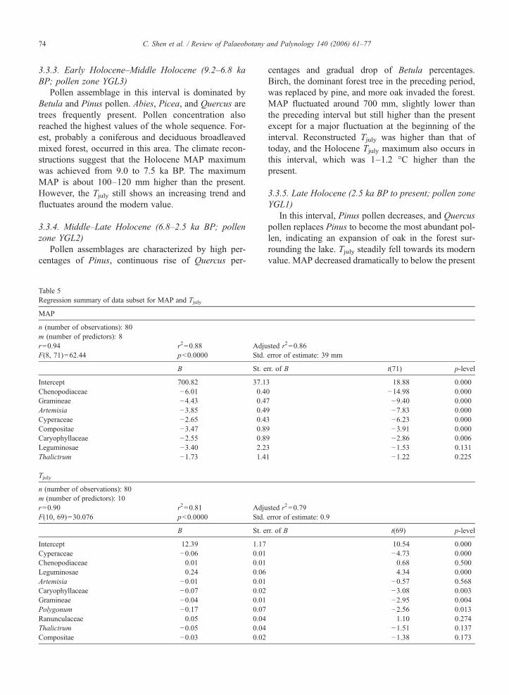
Table 5Regression summary of data subset for MAP and Tjuly

MAP

n (number of observations): 80m (number of predictors): 8r=0.94 r2=0.88 AdjuF(8, 71)=62.44 pb0.0000 Std.

B St. e

Intercept 700.82 37.1Chenopodiaceae −6.01 0.4Gramineae −4.43 0.4Artemisia −3.85 0.4Cyperaceae −2.65 0.4Compositae −3.47 0.8Caryophyllaceae −2.55 0.8Leguminosae −3.40 2.2Thalictrum −1.73 1.4

Tjuly

n (number of observations): 80m (number of predictors): 10r=0.90 r2=0.81 AdjuF(10, 69)=30.076 pb0.0000 Std.

B St. e

Intercept 12.39 1.17Cyperaceae −0.06 0.01Chenopodiaceae 0.01 0.01Leguminosae 0.24 0.06Artemisia −0.01 0.01Caryophyllaceae −0.07 0.02Gramineae −0.04 0.01Polygonum −0.17 0.07Ranunculaceae 0.05 0.04Thalictrum −0.05 0.04Compositae −0.03 0.02

centages and gradual drop of Betula percentages.Birch, the dominant forest tree in the preceding period,was replaced by pine, and more oak invaded the forest.MAP fluctuated around 700 mm, slightly lower thanthe preceding interval but still higher than the presentexcept for a major fluctuation at the beginning of theinterval. Reconstructed Tjuly was higher than that oftoday, and the Holocene Tjuly maximum also occurs inthis interval, which was 1–1.2 °C higher than thepresent.

3.3.5. Late Holocene (2.5 ka BP to present; pollen zoneYGL1)

In this interval, Pinus pollen decreases, and Quercuspollen replaces Pinus to become the most abundant pol-len, indicating an expansion of oak in the forest sur-rounding the lake. Tjuly steadily fell towards its modernvalue. MAP decreased dramatically to below the present

sted r2=0.86error of estimate: 39 mm

rr. of B t(71) p-level

3 18.88 0.0000 −14.98 0.0007 −9.40 0.0009 −7.83 0.0003 −6.23 0.0009 −3.91 0.0009 −2.86 0.0063 −1.53 0.1311 −1.22 0.225

sted r2=0.79error of estimate: 0.9

rr. of B t(69) p-level

10.54 0.000−4.73 0.0000.68 0.5004.34 0.000

−0.57 0.568−3.08 0.003−2.95 0.004−2.56 0.0131.10 0.274

−1.51 0.137−1.38 0.173


value at first, then increased sharply from 1.6 to 1.3 kaBP. It then decreased and increased again to its presentlevel.

4. Discussion and conclusions

Deriving transfer functions is the first step of quanti-tative interpretation of pollen data in climatic terms(Bartlein and Whitlock, 1993; Seppa and Bennett,2003). In this procedure, the most important issue is todecide whether to use linear- or unimodal-based meth-ods for a particular dataset. It is a general rule of naturethat the quantitative relationships between taxa and en-vironmental variables are non-linear, and the abundanceof a taxon is often a unimodal function of the environ-mental variables (Gaussian model) (Birks, 1995). How-ever, a unimodal curve will appear monotonic andapproximately linear if a limited range of the environ-mental variables is covered by samples. The IL regres-sion model requires the assumption that a linearrelationship exists between climatic variables and pollentype (Howe and Webb III, 1983; Bartlein et al., 1985;Birks, 1995). To avoid violating this assumption, se-lection of an adequate geographical region is importantin reducing model specification errors (Bartlein et al.,1985). However, to define an adequate geographicalregion in the Tibetan Plateau as in North America orEurope is difficult due to its landscape complexity, es-pecially in the southern Plateau. In our study, the scatterdiagrams (Figs. 5–8) show that significant linear re-lationships exist between MAP, Tjuly, and most of thepollen types. Thus, the assumption of linearity is sat-isfied in our data. For further testing, we separated asubset of data consisting of samples from meadow,steppe, and desert to develop transfer functions (Table 5).Comparison of regression results shows no markeddifference between them except the data subset withsmaller standard errors of estimates for both MAP andTjuly, and slightly higher r

2 value for Tjuly. However, it isevident that the transfer functions developed by the datasubset could reduce the estimate errors in climatic re-construction. WA-PLS model is a non-linear unimodal(Gaussian)-based technique. It is thus not limited by anygeographic region. Comparison of results from linearmodels and non-linear models seems to show that WA-PLS models have larger estimate errors than linearmodels. One explanation for this discrepancy is thatlinear models almost certainly underestimate the trueuncertainty (Bartlein and Whitlock, 1993; Birks, 1995).

Ecologically, the derived transfer functions are real-istic, as discussed above. Statistically, our analysis alsoindicates that these transfer functions are reliable, as

assessed by two main lines of evidence. First, CCAdemonstrated that pollen–climate relationships in theTibetan Plateau are significant. Second, performancestatistics (r2 and the standard error for IL regressionmodel; r2 and RMSEP for WA-PLS regression model)show that these transfer functions significantly predictobserved MAP and Tjuly. r2 is a common measureof goodness of fit in the transfer function approach(Bartlein and Whitlock, 1993; Seppa and Bennett,2003). The values of r2 for our transfer functions(0.90 and 0.87 for MAP in IL regression model andWA-PLS model respectively; 0.72 and 0.66 for Tjuly) arequite high, and comparable to those of pollen–climatetransfer functions developed in North America and Eu-rope (e.g. Bartlein et al., 1985; Bartlein and Whitlock,1993; Seppa and Birks, 2001; Seppa et al., 2004). Thestandard error is commonly quoted as a measure of thepredictive ability of the training set (Birks, 1995). Thevalues of standard error for MAP are 6.5% and 7%(11.2% and 12% for Tjuly) as percentage of the gradientlength of MAP (Tjuly) in IL and WA-PLS regressionmodels respectively. By comparison with the otherpublished models for pollen or aquatic organisms basedon similar methods (e.g. Bigler and Hall, 2002; Seppa etal., 2004; Rull, 2006), they can be considered low. Thisshows a superior performance of our derived transferfunctions in prediction power.

There are several means of evaluating how reliablethe paleoclimatic estimates are as derived from transferfunctions. The most powerful evaluation procedure isto validate the reconstruction against known historicalrecords or other independent paleoenvironmental re-cords (Birks, 1995). The estimates of MAP and Tjulyfor the top fossil sample are in agreement with theobserved values as mentioned above. It seems to in-dicate that derived transfer functions can provide reli-able paleoclimatic estimates. Comparison with otherindependent paleoenvironmental records is difficult forthe Tibetan Plateau because no quantitative climatereconstruction has been published, although there aresome existing proxy records of temperature and pre-cipitation derived from ice core (e.g. Thompson et al.,1989) and lake sediments (e.g. Van Campo and Gasse,1993). A useful but informal evaluation procedure is toestimate the same climatic parameter by several nu-merical methods (Birks, 1995). In our case study, theclimates reconstructed by transfer functions show anexcellent consistency in estimate values between twodifferent techniques, although the standard errors arelarger in WA-PLS models than IL models due to thereason mentioned above. Additionally, the main trendof climate reconstructions is also consistent with


vegetation succession inferred from pollen data. How-ever, the occurrence of long-distance pollen probablyleads to a bias towards overestimates of MAP and Tjulyfor a few samples such as two basal samples of ZoneYGL6 and the basal sample of Zone YGL5. In sum-mary, our study of quantitative relationships betweenmodern pollen rain and climate in the Tibetan Plateaushows that:

(1) MAP and Tjuly are two dominant factors control-ling the variations in the modern pollen rain, i.e.spatial distribution of modern vegetation.

(2) The transfer functions developed in terms of MAPand Tjuly using IL and WA-PLS regression modelsare reliable in reconstructing paleoclimate quan-titatively based on the fossil pollen data.

Acknowledgment

This research was supported by grants from the U.S.National Science Foundation (NSF grants ATM-9410491, ATM-0081941), The Chinese National Sci-ence Foundation (grants No. 49371068 and 49871078),and dissertation research grants from the GeologicalSociety of America (GSA), Association of AmericanGeographers (AAG), and the Robert C. West FieldResearch Award (LSU Department of Geography andAnthropology). We thank Dr. H.J.B. Birks and Dr.Stephen Juggins for providing the WA-PLS program.We also thank Dr. A. Peter Kershaw for comments onthe manuscript.

References

Andrews, J.T., Mode, W.N., Davis, P.T., 1980. Holocene climate basedon pollen transfer functions, eastern Canadian Arctic. Arctic andAlpine Research 12, 41–64.

Bartlein, P.J., Whitlock, C., 1993. Paleoclimatic interpretation of theElk Lake pollen record. Geological Society of America SpecialPaper 276, 275–293.

Bartlein, P.J., Prentice, I.C.,Webb III, T., 1985. Mean July temperature at6000 yr BP in eastern North America: regression equations forestimates from fossil-pollen data. In: Harington, C.R. (Ed.), ClimaticChange in Canada 5: Critical Periods in the Quaternary ClimaticHistory of Northern North America Syllogeus, vol. 55, pp. 301–342.

Bartlein, P.J., Prentice, I.C., Webb III, T., 1986. Climatic responsesurfaces from pollen data for some eastern North American taxa.Journal of Biogeography 13, 35–57.

Bernabo, J.C., 1981. Quantitative estimates of temperature changesover the last 2700 years in Michigan based on pollen data.Quaternary Research 15, 142–159.

Bigler, C., Hall, R., 2002. Diatoms as indicators of climatic andlimnological change in Swedish Lapland: a 100-lake calibration setand its validation for paleoecological reconstructions. Journal ofPaleolimnology 27, 97–115.

Birks, H.J.B., 1995. Quantitative palaeoenvironmental reconstruc-tions. In: Maddy, D., Brew, J.S. (Eds.), Statistical Modelling ofQuaternary Scicene Data. Technical Guide, vol. 5. QuaternaryResearch Association, Cambridge, pp. 161–254.

Birks, H.J.B., 1998. Numerical tools in quantitative paleolimnology—progress, potentialities, and problems. Journal of Paleolimnology20, 301–332.

Birks, H.J.B., 2003. Quantitative palaeoenvironmental reconstructionsfrom Holocene biological data. In: Mackay, A., Battarbee, R.W.,Birks, H.J.B., Oldfield, F. (Eds.), Global Change in the Holocene.Arnold, London, pp. 107–123.

Birks, H.J.B., Gordon, A.D., 1985. Numerical Methods in QuaternaryPollen Analysis. Academic Press, London. 317 pp.

Fontes, J.-C., Melieres, F., Gibert, E., Liu, Q., Gasse, F., 1993. StableIsotope and radiocarbon balances of two Tibetan Lakes (Sumxi Co,Longmu Co) from 13000 B.P. Quaternary Sciences Reviews 12,875–887.

Fontes, J.-C., Gasse, F., Gibert, E., 1996. Holocene environmentalchanges in Bangong Co Basin (Western Tibet). Part 1: Chronologyand stable isotopes of carbonates of a Holocene lacustrine core.Palaeogeography, Palaeoclimatology, Palaeoecology 120, 25–47.

Guiot, J., 1987. Late Quaternary climatic changes in France estimatedfrom multivariate pollen time series. Quaternary Research 28,100–118.

Guiot, J., 1990. Methodology of the last climatic cycle reconstructionin France from pollen data. Palaeogeography, Palaeoclimatology,Palaeoecology 80, 49–69.

Heusser, C.J., Streeter, S.S., 1980. A temperature and precipitationrecord of the past 16000 years in southern Chile. Science 210,1345–1347.

Howe, S., Webb III, T., 1983. Calibrating pollen data in climatic terms:improving the methods. Quaternary Science Reviews 2, 17–51.

Huntley, B., Prentice, I.C., 1988. July temperatures in Europe frompollen data, 6000 years before present. Science 241, 687–690.

Huntley, B., Prentice, I.C., 1993. Holocene vegetation and climate ofEurope. In: Wright Jr., H.R., Kutzbach, J.E., Webb III, T.,Ruddiman, W.F., Street-Perrott, F.A., Bartlein, P.J. (Eds.), GlobalClimates Since the Last Glacial Maximum. University ofMinnesota Press, Minneapolis, pp. 136–168.

Jongman, R.H.G., ter Braak, C.J.F., van Tongeren, O.F.R., 1987. DataAnalysis in Community and Landscape Ecology. Pudoc,Wageningen.

Liu, K.-b., 1988. Quaternary history of the temperate forests of China.Quaternary Science Reviews 7, 1–20.

Liu, K.-b., Qiu, H.-l., 1994. Late-Holocene pollen records ofvegetational changes in China: climate or human disturbance.Terrestrial, Atmospheric and Oceanic Sciences 5, 393–410.

Markgraf, V., Webb, R.S., Anderson, K.H., Anderson, L., 2002.Modern pollen/climate calibration for southern South America.Palaeogeography, Palaeoclimatology, Palaeoecology 181,375–397.

Overpeck, J.T., Webb III, T., Prentice, I.C., 1985. Quantitativeinterpretation of fossil pollen spectra: dissimilarity coefficientsand the method of modern analogs. Quaternary Research 23,87–108.

Rull, V., 2006. A high mountain pollen–altitude calibration set for pa-laeoclimatic use in the tropical Andes. The Holocene 16, 105–117.

Seppa, H., Bennett, K.D., 2003. Quaternary pollen analysis: recentprogress in palaeoecology and palaeoclimatology. Progress inPhysical Geography 27, 548–579.

Seppa, H., Birks, H.J.B., 2001. July mean temperature and annualprecipitation trends during the Holocene in the Fennoscandian


tree-line area: pollen-based climate reconstructions. The Holocene11, 527–539.

Seppa, H., Birks, H.J.B., Odland, A., Posta, A., Veski, S., 2004. Amodern pollen–climate calibration set from northern Europe:developing and testing a tool for palaeoclimatological reconstruc-tions. Journal of Biogeography 31, 251–267.

Shen, C., 2003. Millennial-scale variations and centennial-scale eventsin the southwest Asian monsoon: pollen evidence from Tibet. PhDDissertation, Louisina State University, Baton Rouge. 286 pp.

Shen, C., Tang, L., 1992. Holocene climate based on pollen transferfunction in Changbaishan mountain and Xiaoxinanling Ranges.In: Shi, Y., Kong, Z. (Eds.), Climate and Environment duringHolocene Megathermal in China. China Ocean Press, Beijing, pp.34–39.

Sibson, R., 1981. A brief description of natural neighbour interpola-tion. In: Barnett, V. (Ed.), Interpreting Multivariate Data. JohnWiley, Chichester, pp. 21–36.

Song, C., Lu, H., Sun, X., 1997. Establishment and application ofpollen–climate transfer functions in North China. Chinese ScienceBulletin 42, 2182–2186.

Swain, A.M., Kutzbach, J.E., Hastenrath, S., 1983. Estimates ofHolocene precipitation for Rajasthan, India based on pollen andlake-level data. Quaternary Research 19, 1–17.

ter Braak, C.J.F., 1986. Canonical correspondence analysis: a neweigenvector technique for multivariate direct gradient analysis.Ecology 67, 1167–1179.

ter Braak, C.J.F., 1987. The analysis of vegetation–environmentrelationships by canonical correspondence analysis. Vegetatio 69,69–77.

ter Braak, C.J.F., Juggins, S., 1993. Weighted averaging partial leastsquares regression (WA-PLS): an improved method for recon-structing environmental variables from species assemblages.Hydrobiologia 269/270, 485–502.

ter Braak, C.J.F., Juggins, S., Birks, H.J.B., van der Voet, H., 1993.Weighted averaging partial least squares regression (WA-PLS):definition and comparison with other methods for species–

environmental calibration. In: Patil, G.P., Rao, C.R9 (Eds.),Multivariate Environmental Statistics. Elsevier Science Publishers,Amsterdam, pp. 525–560.

Thompson, L.G., Mosley-Thompson, E., Davis, M.E., Bolzan, J.F.,Dai, J., Yao, T., Gundestrup, N., Wu, X., Klein, Z., Xie, Z., 1989.Holocene–Late Pleistocene Climatic ice core records fromQinghai–Tibetan Plateau. Science 246, 474–477.

Van Campo, E., Gasse, F., 1993. Pollen- and diatom-inferred climaticand hydrological changes in Sumxi Co Basin (Western Tibet) since13,000 yr B.P. Quaternary Research 39, 300–313.

Wang, F., Song, C., Sun, X., Cheng, Q., 1997. Climatic responsesurface from pollen data for four arboreal taxa in North China.Acta Botanica Sinica 39, 272–281.

Webb III, T., Bryson, R.A., 1972. Late- and post-glacial climaticchange in the northern Midwest, USA: quantitative estimatesderived from fossil pollen spectra by multivariate statisticalanalysis. Quaternary Research 2, 70–115.

Webb III, T., Clark, D.R., 1977. Calibrating micropaleontological datain climatic terms: a critical review. Annals of the New YorkAcademy of Science 288, 93–118.

Webb, R.S., Anderson, K.H., Webb, T., 1993a. Pollen response-surface estimates of late-Quaternary changes in the moisturebalance of northeastern United States. Quaternary Research 40,213–227.

Webb III, T., Ruddiman, W.F., Street-Perrott, F.A., Markgraf, V.,Kutzbach, J.E., Bartlein, P.J., Wright Jr., H.R., Prell, W.L., 1993b.Climatic changes during the past 18,000 years: regional syntheses,mechanisms, and causes. In: Wright Jr., H.R., Kutzbach, J.E.,Webb III, T., Ruddiman, W.F., Street-Perrott, F.A., Bartlein, P.J.(Eds.), Global Climates Since the Last Glacial Maximum.University of Minnesota Press, Minneapolis, pp. 514–535.

Webb III, T., Anderson, K.H., Bartlein, P.J., Webb, R.S., 1998. LateQuaternary climate change in eastern North America: a compar-ison of pollen-derived estimates with climate model results.Quaternary Science Reviews 17, 587–606.

quantitative relationships between modern pollen rain and ... · quantitative relationships between...

Documents