AFRL-IF-RS-TR-2006-216 Final Technical Report June 2006 QUANTUM APPROACHES TO LOGIC CIRCUIT SYNTHESIS AND TESTING

University of Michigan

Sponsored by Defense Advanced Research Projects Agency DARPA Order No. L486

APPROVED FOR PUBLIC RELEASE; DISTRIBUTION UNLIMITED The views and conclusions contained in this document are those of the authors and should not be interpreted as necessarily representing the official policies, either expressed or implied, of the Defense Advanced Research Projects Agency or the U.S. Government.

AIR FORCE RESEARCH LABORATORY INFORMATION DIRECTORATE

ROME RESEARCH SITE ROME, NEW YORK

STINFO FINAL REPORT

This report has been reviewed by the Air Force Research Laboratory, Information Directorate, Public Affairs Office (IFOIPA) and is releasable to the National Technical Information Service (NTIS). At NTIS it will be releasable to the general public, including foreign nations.

AFRL-IF-RS-TR-2006-216 has been reviewed and is approved for publication APPROVED: /s/

STEVEN DRAGER Project Engineer

FOR THE DIRECTOR: /s/

JAMES A. COLLINS Deputy Chief, Advanced Computing Division Information Directorate

REPORT DOCUMENTATION PAGE Form Approved OMB No. 0704-0188

Public reporting burden for this collection of information is estimated to average 1 hour per response, including the time for reviewing instructions, searching data sources, gathering and maintaining the data needed, and completing and reviewing the collection of information. Send comments regarding this burden estimate or any other aspect of this collection of information, including suggestions for reducing this burden to Washington Headquarters Service, Directorate for Information Operations and Reports, 1215 Jefferson Davis Highway, Suite 1204, Arlington, VA 22202-4302, and to the Office of Management and Budget, Paperwork Reduction Project (0704-0188) Washington, DC 20503. PLEASE DO NOT RETURN YOUR FORM TO THE ABOVE ADDRESS. 1. REPORT DATE (DD-MM-YYYY)

JUNE 2006 2. REPORT TYPE

Final 3. DATES COVERED (From - To)

May 01 – Dec 05 5a. CONTRACT NUMBER

F30602-01-2-0520

5b. GRANT NUMBER

4. TITLE AND SUBTITLE QUANTUM APPROACHES TO LOGIC CIRCUIT SYNTHESIS AND TESTING

5c. PROGRAM ELEMENT NUMBER 62712E

5d. PROJECT NUMBER L486

5e. TASK NUMBER LC

6. AUTHOR(S) John P. Hayes, Igor L. Markov

5f. WORK UNIT NUMBER ST

7. PERFORMING ORGANIZATION NAME(S) AND ADDRESS(ES) University of Michigan EECS Department 2260 Hayward Ann Arbor Michigan 48109

8. PERFORMING ORGANIZATION REPORT NUMBER N/A

10. SPONSOR/MONITOR'S ACRONYM(S)

9. SPONSORING/MONITORING AGENCY NAME(S) AND ADDRESS(ES) Defense Advanced Research Projects Agency AFRL/IFTC 3701 North Fairfax Drive 525 Brooks Road Arlington Virginia 22203-1714 Rome New York 13441-4505 11. SPONSORING/MONITORING

AGENCY REPORT NUMBER AFRL-IF-RS-TR-2006-216

12. DISTRIBUTION AVAILABILITY STATEMENT APPROVED FOR PUBLIC RELEASE; DISTRIBUTION UNLIMITED. PA#06-445

13. SUPPLEMENTARY NOTES

14. ABSTRACT The overall objective of this project was to investigate quantum study computing concepts in an integrated way and apply design automation techniques, such as synthesis, simulation and testing, to quantum logic circuits via mathematical and algorithmic models implemented in software. The research considered the interplay between conventional and quantum logic design, aiming at a deeper understanding of both areas and provided extensive computational experimentation at scales uncommon in quantum computing research. The project’s main accomplishments included the development of efficient and practical synthesis methods for quantum circuits, which resulted in near-optimal automatic synthesis algorithms for n-qubit reversible circuits; new theoretical results on optimal quantum computations; and improved high performance simulation techniques through a new data representation for quantum circuits, the quantum information decision diagram (QuIDD) and a simulator program, QuIDDPro, which is currently the highest-performance simulator in its class. 15. SUBJECT TERMS Quantum Computing, Circuit Synthesis, Simulation, Testing

16. SECURITY CLASSIFICATION OF: 19a. NAME OF RESPONSIBLE PERSON Steven Drager

a. REPORT U

b. ABSTRACT U

c. THIS PAGE U

17. LIMITATION OF ABSTRACT

UL

18. NUMBER OF PAGES

61 19b. TELEPONE NUMBER (Include area code)

i

Table of Contents

1. Executive Summary 1

2. Introduction 2

3. Synthesis of Quantum Circuits 14

4. Simulation of Quantum Circuits 30

5. Publications 52

ii

List of Figures

Figure 1: Reversible quantum half-adder circuit. 8

Figure 2: Matrix form of the quantum half-adder. 9

Figure 3: (a) A logic function, (b) its BDD representation, (c) its BDD representation

after applying the first reduction rule, and (d) its ROBDD representation. 10

Figure 4: The three recursive rules used by the Apply operation with xi = Var(vf),

xj = Var(vg) and xi < xj meaning that that xi precedes xj in the variable ordering. 11

Figure 5: A typical quantum logic circuit. Information flows from left to right, and

the higher wires represent higher order qubits. The quantum operation performed by

this circuit is (U7 ⊗ U8 ⊗ U9)(I2 ⊗ V3)(V2 ⊗ I2)(U4 ⊗ U5 ⊗ U6)(I2 ⊗ V1)(U1 ⊗ U2 ⊗ U3),

and the last factor is outlined above. 17

Figure 6: The recursive decomposition of a multiplexed Rz gate. The boxed CNOT

gates may be canceled. 22

Figure 7: Implementing a long-range CNOT gate with nearest-neighbor CNOTs. 27

Figure 8: Sample QuIDDs for state vectors of (a) best, (b) worst and (c) mid-range

size. 31

Figure 9: (a) A 2-qubit Hadamard matrix and (b) its QuIDD multiplied by |00 =

(1,0,0,0). 31

Figure 10: General form of a tensor product between two QuIDDs A and B. 35

Figure 11: Circuit-level implementation of Grover’s algorithm. 38

Figure 12: Probability of successful search for one, two, four and eight items as a

function of the number of iterations after which the measurement is performed. 44

Figure 13: (a) QuIDD for the density matrix resulting from U|01 01|U!, where

iii

U = H ⊗ H, and (b) its explicit matrix form. 46

Figure 14: Pseudo-code for (a) the QuIDD outer product and (b) its complex

conjugation helper function Complex_Conj. 47

Figure 15: Quantum circuit for the bb84Eve benchmark. 49

iv

List of Tables

Table 1: A comparison of CNOT counts for unitary circuits generated by several

algorithms (best results are in bold). We have labeled the algorithms by the matrix

decomposition they implement. The results of our work are boldfaced, including

an optimized QR decomposition and three algorithms based on the Quantum

Shannon Decomposition(QSD). 26

Table 2: Size of QuIDDs (number of nodes) for Grover’s algorithm. 41

Table 3: Simulating Grover's algorithm with n qubits using Octave (Oct), MATLAB

(MAT), Blitz++ (B++) and QuIDDPro (QP) with Oracle Design 1. 42

Table 4: Simulating Grover's algorithm with n qubits using Octave (Oct), MATLAB

(MAT), Blitz++ (B++) and QuIDDPro (QP) with Oracle Design 2. 43

Table 5: Number of Grover iterations at which [5] predict the highest probability of

measuring one of the items sought. 44

Table 6: Performance results for QCSim and QuIDDPro on error-related benchmarks (MEM-OUT indicates that a memory usage cutoff of 2GB was exceeded). 50

1

1. Executive Summary The overall objective of this project was to study quantum computing (QC) concepts in an integrated way and apply design automation techniques, such as synthesis, simulation and testing to quantum logic circuits via mathematical and algorithmic models implemented in software. The project considers the interplay between conventional and quantum logic design issues, with the goal of obtaining a deeper understanding of both areas. The approach employed is not limited to particular circuit styles, and is useful for a variety of implementation technologies. A key feature of this effort is extensive computational experimentation at scales uncommon in QC research. In the course of this project we obtained a deeper understanding of the relation between the computer-aided design (CAD) requirements for classical and quantum computing. We concluded that quantum design automation (QDA) is a necessary enabling factor in achieving scalable classical and quantum circuits. The project’s main accomplishments include the development of efficient and practical synthesis methods for quantum circuits, new theoretical results on optimal quantum computations, and improved high-performance simulation techniques. Our early work on reversible circuits (quantum circuits are required to be reversible) proved that a well-known result of Toffoli’s on odd permutations cannot be improved. We also contributed synthesis algorithms for reversible circuits and statistical studies of optimal circuits that are now commonly cited. In July 2004, our paper on reversible circuit synthesis in the IEEE Transactions on CAD received the IEEE’s Donald O. Pederson Best Paper Award. For n-qubit operators, our algorithms can synthesize automatically the best known circuit so far, and are within a factor of two of the optimum (which existing techniques cannot yet find in general). For two-qubit circuits, we obtained a comprehensive classification that allows one to achieve optimal CNOT counts for every possible input operator. In quantum circuit simulation, we introduced a new data representation for QC vectors and matrices, the quantum information decision diagram (QuIDD). Using QuIDDs, we implemented a high-performance quantum simulation program QuIDDPro, which is being used by about 20 research groups in the U.S. and elsewhere. QuIDDPro remains the highest-performance simulator in its class. We published a substantial number of papers on our research, and created a website http://proton.eecs.umich.edu/UMQuS to facilitate the use of our algorithms via the Word Wide Web. We interacted with experimentalists at the University of Michigan and elsewhere who work on implementation of quantum circuits. We also cooperated with other QuIST-sponsored QC researchers at NIST, LANL, MIT and Columbia. In addition, we made efforts to popularize QC research in the broader CAD design community via talks and tutorials at various conferences and universities in the U.S. and Europe.

2

2. Introduction

The physics Nobel Laureate Richard Feynman observed in the 1980s that simulating quantum mechanical processes on a standard or classical computer seems to require super-polynomial memory and time [8]. For instance, a complex vector of size 2n is needed to represent all the information in n quantum states, and square matrices of size 22n are needed to model (simulate) the time evolution of the states [11, 13]. Consequently, Feynman proposed quantum computing, which uses the quantum mechanical states themselves to simulate quantum processes. The key idea is to replace bits with quantum states called qubits as the fundamental units of information. A quantum computer can operate directly on exponentially more data than a classical computer with a similar number of operations and information units.

Since Feynman's day, various practical information processing applications that exploit quantum mechanical effects have been proposed. QC algorithms have been discovered to quickly search unstructured databases [7], and to factor numbers in polynomial time [15]. Implementing such quantum algorithms has proven very difficult, however, in part due to errors caused by the environment [9, 12]. Quantum mechanics has been successfully employed to enable secure key exchange for encrypted communication since the act of eavesdropping can be detected as destructive measurement on quantum states [2, 3]. A related application is the design of reversible logic circuits. The operations performed on qubits in quantum computation must be unitary, so they are all invertible and allow re-derivation of the inputs given the outputs. This phenomenon gives rise to a host of potential applications in fault-tolerant computation. Since reversible logic, secure quantum communication, and quantum algorithms can be modeled as quantum circuits [13], the quantum analogue of digital logic circuits, quantum circuit simulation could be of major benefit to these applications. In fact, any quantum mechanical phenomenon with a finite number of states can be modeled as a quantum circuit. Unfortunately, the very problem which brought forth quantum mechanics as a useful computational tool is the same problem which, in general, renders quantum circuit simulation on a classical computer intractable.

We have investigated the synthesis of efficient quantum logic circuits which perform two tasks: implementing generic quantum computations and initializing quantum registers. In contrast to conventional computing, the latter task is nontrivial because the state-space of an n-qubit register is not finite and contains exponential superpositions of classical bit strings. As a special case, we have analyzed the case of 2-qubit circuits and identified circuit topologies that can implement any unitary 2-qubit quantum computation with up to 3 CNOT gates. Our circuit synthesis work is reported in detail in Section 3 of this report.

Software simulation has long been a valuable tool for the design and testing of classical digital circuits. This problem too was once thought to be computationally intractable. Early simulation and synthesis techniques for n-bit circuits often required O (2n) runtime and memory, with the worst-case complexity being typical. Later algorithmic advancements ushered in the ability to perform circuit simulation much more efficiently in practical cases. One such advance was the development of a data structure called the reduced ordered binary decision diagram (ROBDD) [5],

3

which can greatly compress the Boolean description of digital circuits and allow direct manipulation of the compressed form. Simulation may also play a vital role in the development of quantum hardware by enabling the modeling and analysis of large-scale designs that cannot be implemented physically with current technology. Unfortunately, straightforward simulation of quantum designs by classical computers executing standard linear-algebraic routines requires O (2n) time and memory [8, 13]. However, just as ROBDDs and other innovations have made the simulation of large classical computers tractable, new algorithms can allow the efficient simulation of quantum computers in many important cases.

Interestingly, if a classical computer can simulate a quantum computer that is solving a particular problem, then the classical computer is computationally as powerful as the quantum computer for the problem in question. Therefore, by discovering new classical algorithms that efficiently simulate quantum computers in certain cases, we can probe the limits of QC. In light of this, it might seem that simulation for the sake of improving quantum hardware introduces competing goals. However, the error correction schemes developed via efficient classical simulation apply, in principle, to other QC tasks that cannot be simulated efficiently. Such simulation can be used as a tool to address the following issues:

1. Characterizing the effect of various errors in practical quantum circuits.

2. Developing and testing multi-qubit error correction techniques to cope with such errors.

3. Exploring the boundaries between the quantum and classical computational models.

In the course of this project, we conducted a large body of research addressing these topics. This resulted in the development of the Quantum Information Decision Diagram (QuIDD), which facilitates efficient simulation of a non-trivial class of quantum circuits [17 - 21]. QuIDDs are discussed in detail later. We also devised significant extensions to the QuIDD data structure that enable efficient simulation with density matrices, which form's a useful tool for incorporating error effects. In addition to QuIDDs, we enlisted a variant of Vidal's simulation method [22] to accurately characterize the effects of gate and systematic error in a quantum circuit that generates remotely entangled EPR pairs. An interesting point about QuIDDs and Vidal's technique is that they can achieve efficient simulation without approximation. Our quantum simulation research is discussed further in Section 4 of this report.

Postulates. Next we outline the basic concepts of quantum computation and quantum circuits. We also discuss the ROBDD data structure, which is required to understand our work involving QuIDDs. Quantum computing is grounded in quantum mechanics, which is governed by four fundamental postulates. Any simulation of QC must implement these postulates in some form if true quantum behavior is to be modeled [13, 14].

Postulate 1. Quantum states are represented as vectors in a Hilbert space.

Since the vectors that arise in quantum computing have finite size, the Hilbert space of quantum states is a complex-numbered vector space with an inner product. This means that qubits, which are quantum states, are represented as vectors for which we can compute inner products. Two low-energy stable states are used to represent the classical values 0 and 1 and are referred to as

4

computational basis states. Like an analog signal, the range of qubit values is a continuum of values between 0 and 1. However, unlike an analog signal, these values denote a probability of obtaining a 0 or 1 upon measurement of a qubit. More formally, given a state vector for some qubit

=Ψ

βα in the standard Dirac notation, α and β are complex numbers (probability amplitudes)

and 122 =+ βα .

2α and 2β are the probabilities of measuring the qubit as a 0 and as a 1,

respectively. One can think of α as the amount of “zeroness” and β as the amount of “oneness'”

that the qubit contains. The basis states 0 and 1 have the form

=

01

0 and

=

10

1 , respectively.

Postulate 2. Operations on quantum states in a closed system are represented using matrix-vector multiplication of the quantum state vector by a unitary matrix.

This postulate describes special types of matrices that are analogous to logic gates in classical computation. A unitary matrix has the property that its adjoint equals its inverse. (The adjoint of a matrix is its complex conjugate transpose.) Unitary matrices are operators which can be used to modify the values of qubits like logic gates, so the terms operator and gate are used interchangeably. Unlike classical logic gates, however, all quantum operators are reversible. Thus, by keeping track of the operations performed on a set of qubits, any quantum computation can be reversed by applying the adjoint of each operation in reverse order. An example of a commonly used operator in quantum computing is the Hadamard operator which has the form

−=

2

1

2

12

1

2

1

H

This operator is frequently used to put a qubit into an equal superposition of 0 and 1.

Postulate 3. Measurement of a quantum state Ψ involves a special set of operators. When such

an operator Ωis applied to Ψ , the result will be one of the eigenvalues of Ω with a certain

probability. Measurement is destructive and changes the measured state Ψ to ω .

In the QC context, this postulate has two main consequences. The first is that measuring the value of a qubit destroys its quantum state, forcing it to a classical 0 or 1 value. The second consequence is that measurement is probabilistic. There are several different types of measurement, but the one that is most pertinent to this discussion is measurement in the computational basis. This involves measuring with respect to the 0 and 1 basis states of a qubit, forcing the qubit to a classical 0 or 1. The actual outcome depends on the probability amplitudes in the superposition of the qubit.

Another form of “measurement” can and often does occur prematurely in quantum systems. This comes in the form of interference from the environment surrounding the qubits and is known as decoherence. In practice, it is difficult to isolate stable quantum states from the environment, and since measurement of any kind is destructive, a computation can easily be ruined before it

5

completes. This problem is one of the greatest technological hurdles facing the physical realization of quantum computers [9, 12, 13].

Postulate 4. Composite quantum states are represented by the tensor product of the component quantum states, and operators that act on composite states are represented by the tensor product of their component matrices.

This postulate enables the description of multiple qubits and multi-qubit operators via a single state vector and matrix, respectively. The tensor product is a standard linear algebraic operation. Given two matrices (vectors) A and B of dimensions MA × NA and MB × NB, respectively, the tensor product A ⊗B multiplies each element of A by the entire matrix (vector) B to produce a new matrix (vector) of dimensions MAMB × NANB. To illustrate, the tensor product of two complex-numbered

vectors

=

b

aV and

=

d

cW is given by

=⊗

bd

bc

ad

ac

WV

In general, there is no restriction on the dimensions of tensor product operands. Matrices of different dimensions can be tensored together, as can vectors and matrices. However, in the quantum domain, we typically compute the tensor product of square, power-of-two-sized matrices to create larger operators (postulate 2), and also the tensor product of power-of-two-sized vectors to create larger composite quantum states (postulate 1). Dirac notation offers a simple short-hand description of composite quantum states in which the state symbols are simply placed side-by-side within a single ket. For the preceding example, the Dirac form is VW . To illustrate the construction of composite quantum operators, we turn to an example involving the Hadamard operator. A Hadamard operator that can be applied to two qubits is constructed via the tensor product of two Hadamard matrices:

−−

−−

−−=

−⊗

−

2

1

2

1

2

1

2

12

1

2

1

2

1

2

12

1

2

1

2

1

2

12

12

12

12

1

2

1

2

12

1

2

1

2

1

2

12

1

2

1

The above examples show that n qubits can be represented by n - 1 tensor products of single qubit vectors, and operators that act on n qubits can be represented by n - 1 tensor products of single qubit operators. The size of a state vector resulting from a series of tensor products on n single qubit vectors is 2n. Similarly, the size of a composite operator which can be applied to n qubits is a

6

matrix of size 22n. It is postulate 4 which gives rise to the exponential complexity of simulation of quantum behavior on classical computers. A straightforward linear algebraic approach to such simulation would have time and memory complexity O (22n) for an n-qubit system.

Properties. An interesting property of quantum states is that they cannot be arbitrarily copied [13]. This points to another fundamental difference between quantum and classical computing. In classical logic circuits, a wire can fan out from the output of a gate and feed into many other gates. This is not possible in the quantum domain for an arbitrary qubit. However, this is not a limitation because quantum states that are known to be orthogonal to each other (including the computational basis states) can be copied. However, if it is known that the quantum states are orthogonal, they can be copied. This implies that the computational basis states 0 and 1 can be copied. Since these states are analogous to the classical bit values 0 and 1, the no-cloning theorem demonstrates that quantum computers are at least as powerful as classical computers.

A standard quantum operator used to copy computational basis states (among other functions) is called the CNOT or controlled-NOT operation. It is a unitary matrix (in accordance with postulate 2) that acts on two qubits. One is the control qubit while the other is the target qubit. When the control qubit is in the 1 state, the CNOT is “activated”, and the state of the target qubit is flipped

from 0 to 1 or vice-versa. If the control qubit is in the 0 state, the target qubit is unchanged. When both the control and target qubits are in the computational basis states, CNOT performs the same function as the classical XOR gate where the target qubit receives the value of the XOR of the control qubit and the old target qubit value. To demonstrate, a CNOT operator is shown below changing the state vector 10 to 11 .

=

1000

0100

0100100000100001

An extension of CNOT is the Toffoli operator, which is basically a CNOT with two control qubits and one target qubit. In this case, the value of the target qubit is flipped if both control qubits are in 1 state. Hence given two control qubits a and b and a target qubit c, the Toffoli gate causes c to

become c ⊕ ab. The Toffoli gate is universal in the sense that it can affect any form of classical computation.

Yet another interesting property of quantum states is entanglement. Two quantum states are entangled if the measurement outcome of one state affects the measurement statistics of the other state. A simple example of entangled states is the Bell state or EPR pair. Suppose two parties, Alice and Bob, each have their own qubit, and the state of both qubits together is given as

BAAB 00=Ψ , where the subscript A denotes the portion of the state due to Alice's qubit, and the subscript B denotes the portion due to Bob's qubit. An EPR pair can be generated from this state by applying a Hadamard gate and a CNOT gate as follows:

7

)1100(2

100))(( BABABAEPR IHCNOT +=⊗=Ψ

The utility of this state lies in the fact that if Alice measures her particle and obtains a 0, then Bob will subsequently also obtain a 0 upon measurement of his particle (the same holds true for a measurement of 1). Once the EPR pair is created, the measurement outcomes of each qubit are correlated even if Alice and Bob physically separate their qubits by any distance. As a result, entanglement has applications in quantum teleportation [4] and secure public key exchange [2, 3].

Density Matrix Representation. An important extension of the state vector is the density matrix. In general, the density matrix for a quantum system is defined as iiii p ΨΨΣ=ρ , where i iterates over each state vector in the quantum system, and pi is the probability of obtaining some state vector iΨ from the system. For the purposes of quantum circuit simulation, however, it is

sufficient to define an n-qubit density matrix as ii ΨΨ=ρ , where iΨ is a state vector for a

sequence of n initialized qubits, and iΨ is its complex-conjugate transpose. In other words, ρ is a

2n ×2n matrix constructed by multiplying a 2n-element column vector by a 2n-element row vector. This operation is also known as the outer product. To illustrate, when iΨ is a single qubit,

[ ]

=

=ΨΨ=

****

**bbba

abaaba

b

aρ

Like the state vector model, a gate operation U can be applied to a density matrix, but it takes the form UρU+, where U+, is the complex-conjugate transpose of the matrix for U.

Perhaps the most useful property of the density matrix is that it can accurately represent a subset of the qubits in a circuit. One can extract this subset of information with the partial trace operation, which produces a smaller matrix, called the reduced density matrix. To understand how this extraction is done, consider the following example in which a 1-qubit operator U is applied to two qubits Ψ and Φ . The density matrix version of this operator is

Φ′Ψ′Φ′Ψ′=⊗ΨΦΨΦ⊗ +)()( UUUU

The state of Φ alone after U is applied, for instance, can be extracted with the partial trace

operation ++ ΦΦΨΨ UUUUtr )( . Here tr is the standard trace operation, which produces a single complex number that is the sum of the diagonal elements of a matrix. Note that the partial trace “traces over” the qubit that is not wanted, leaving behind the desired qubit states. Using the partial trace to extract information about subsets of qubits in a circuit is invaluable in simulation. Many practical quantum circuits contain ancillary qubits which help to perform an intermediate function in the circuit but contain no useful information at the output of the circuit. The partial trace therefore allows a simulation to report the density matrix information only for the qubits that contain useful data.

8

Another application of the partial trace in quantum circuits is the modeling of noise from the environment. Coupling between the environment and data qubits can be modeled as the tensor product of data qubits with quantum states controlled by the environment [13]. In such a situation, the partial trace can be used to extract the state of data qubits after being affected by noise. For these reasons and others, it is crucial that a quantum simulator support the density matrix representation.

Figure 1: Reversible quantum half-adder circuit

Quantum Circuits. These are analogous to circuits at the logic design level of classical computation, and it is standard practice to model quantum computation at the quantum circuit level. The two major components in a quantum circuit are the qubits (postulate 1) and the operators or gates (postulate 2). The values of the qubits are observed through measurement (postulate 3), and multiple qubits and gates can be expressed via the tensor product (postulate 4). Clearly, the postulates of quantum mechanics provide a complete set of properties with which to perform logic design subject to the fanout constraint of the no-cloning theorem. In the remainder of this subsection, we cover two small quantum circuit examples to familiarize the reader with the standard quantum circuit notation.

The first example, shown in Figure 1 shows a quantum half-adder. It performs the same function as the standard half-adder in classical logic circuits when the inputs are all in the computational basis. Notice that the qubits are depicted graphically as parallel, horizontal lines. These lines can be thought of as wires, but they actually represent the evolution of the qubits over time. Gates are depicted as objects placed on top of the horizontal qubit lines, affecting only those qubits lines that they are in contact with graphically, similar to a classical logic gate. The spacing between gates on the qubit lines has no significance. The only important aspect of gate placement is whether one gate appears before another, implying an order of operations to be performed on the affected qubits. The quantum half-adder simply consists of a Toffoli gate G1 affecting all three qubits followed by a CNOT gate G2) affecting the first two qubits only. The solid circles represent inputs for the control qubits, while the unfilled circles represent inputs/outputs for the target qubits. In general, the input qubits are placed at the left end of the qubit lines, with the final output state of the qubits appearing at the right end. The matrix representation of the half-adder gates is given in Figure 2. Note that although the circuit diagram flows in a left to right fashion, that is, gate G1 is applied before gate G2, the matrices representing the unitary operators are applied in a seemingly reverse order.

9

The Toffoli and CNOT gates play an important role in universal quantum gate sets. Analogous to their classical digital counterparts, universal quantum gate sets can be used to implement any quantum computation. However, discrete universal quantum gate sets can only approximate arbitrary quantum computations, though the approximation can achieve any desired level of accuracy. One example of a discrete universal quantum gate set consists of the Hadamard, phase, CNOT, and π/8 gates [13]. Another discrete universal quantum gate set consists of the Hadamard, phase, CNOT, and Toffoli gates. In contrast, universal quantum gate sets containing an infinite number of gates enable an exact decomposition of any quantum computation. One such gate set consists of the CNOT gate and the infinite set of all 1-qubit unitary operators. Interestingly, given a circuit consisting of gates from this infinite set, the Solovay-Kitaev theorem proves that an approximation with accuracy ε can be achieved using the aforementioned discrete gate sets with only polylogarithmically more gates in terms of the number of CNOTs in the original circuit and ε [10].

( )

⊗

=⊗=

0100000010000000001000000001000000001000000001000000001000000001

1001

0100100000100001

_ TICAdderHalf

Figure 2: Matrix form of the quantum half-adder.

Binary Decision Diagrams. The binary decision diagram (BDD) was introduced by Lee in the 1950s in the context of classical logic circuit design. This data structure represents a Boolean function f(x1,x2,...,xn) by a directed acyclic graph (DAG); see Figure 3. By convention, the top node of a BDD is labeled with the name of the function f represented by the BDD. Each variable xi of f is then associated with one or more nodes that each has two outgoing edges labeled then (solid line) and else (dashed line). The then edge of node xi denotes an assignment of logic 1 to xi, while the else edge represents an assignment of logic 0. These nodes are called internal nodes and are labeled by the corresponding variable xi. The edges of the BDD point downward, implying a top-down assignment of values to the Boolean variables.

At the bottom of the BDD are terminal nodes containing the logic values 0 or 1. They denote the output value of the function f for a given assignment of its variables. Each path through the BDD from top to bottom represents a specific assignment of 0-1 values to the variables x1,x2,...,xn of f, and ends with the corresponding output value f(x1,x2,...,xn) appearing at one of the BDD’s terminal nodes.

10

Figure 3: (a) A logic function, (b) its BDD representation, (c) its BDD representation after applying the first reduction rule, and (d) its ROBDD representation.

The original BDD data structure conceived by Lee has exponential memory complexity ( )n2Θ , where n is the number of Boolean variables in a given logic function. Moreover, exponential memory and runtime are required in many practical cases, making this data structure impractical for simulation of large logic circuits. To address this limitation, Bryant developed the reduced ordered BDD (ROBDD) [5], where all variables are ordered, and decisions are made in that order. A key advantage of the ROBDD is that variable-ordering facilitates an efficient implementation of reduction rules that automatically eliminate redundancy from the basic BDD representation and may be summarized as follows:

1. There are no nodes v and v’ such that the subgraphs rooted at v and v’ are isomorphic.

2. There are no internal nodes with then and else edges that both point to the same node.

An example of how the rules transform a BDD into an ROBDD is shown in Figure 3. The subgraphs rooted at the x1 nodes in Figure 3b are isomorphic. By applying the first reduction rule, the BDD in Figure 3b is converted into the BDD in Figure 3c. In this new BDD, the then and else edges of the x0 node now point to the same node. Applying the second reduction rule eliminates the x0 node, producing the ROBDD in Figure 3d. Intuitively it makes sense to eliminate the x0 node since the output of the original function is determined solely by the value of x1. An important aspect of redundancy elimination is the sensitivity of ROBDD size to the variable ordering. Finding the optimal variable ordering is an NP-complete problem, but efficient ordering heuristics have been developed for specific applications. Moreover, it turns out that many practical logic functions have ROBDD representations that are polynomial (or even linear) in the number of input variables. Consequently, ROBDDs have become indispensable tools in the design and simulation of classical logic circuits.

Even though the ROBDD is often quite compact, efficient algorithms are necessary to make it practical for circuit simulation. Thus, in addition to the foregoing reduction rules, Bryant introduced a variety of ROBDD operations whose complexities are bounded by the size of the

11

ROBDDs being manipulated. Of central importance is the Apply operation, which performs a binary operation with two ROBDDs, producing a third ROBDD as the result. It can be used, for example, to compute the logical AND of two functions. Apply is implemented by a recursive traversal of the two ROBDD operands. For each pair of nodes visited during the traversal, an internal node is added to the resultant ROBDD using the three rules depicted in Figure 4. To understand the rules, some notation must be introduced. Let v denote an arbitrary node in an ROBDD f If v is an internal node, Var(vf) is the Boolean variable represented by vf, T(vf) is the node reached when traversing the then edge of vf, and E(vf) is the node reached when traversing the else edge of vf.

Figure 4: The three recursive rules used by the Apply operation with xi = Var(vf), xj = Var(vg) and xi < xj meaning that that xi precedes xj in the variable ordering.

Clearly the rules depend on the variable ordering. The recursion stops when both vf and vg are terminal nodes. When this occurs, the current operation op is performed with the values of the terminals as operands, and the resulting value is added to the ROBDD result as a terminal node. For example, if vf contains the value logical 1, vg contains the value logical 0, and op is defined to be ⊕ or XOR, then a new terminal with value 1 ⊕ 0 = 1 is added to the ROBDD result. Terminal nodes are considered after all variables are considered. Thus, when a terminal node is compared to an internal node, either Rule 1 or Rule 2 will be invoked depending on which ROBDD the internal node is from.

The success of ROBDDs in making a seemingly difficult computational problem tractable in practice led to the development of ROBDD variants outside the domain of logic design. Of particular relevance to this work are multi-terminal binary decision diagrams (MTBDDs) [6] and algebraic decision diagrams (ADDs) [1]. These data structures are compressed representations of matrices and vectors rather than logic functions, and the amount of compression achieved is proportional to the frequency of repeated values in a given matrix or vector. Additionally, some standard linear-algebraic operations such as matrix multiplication are defined for MTBDDs and ADDs. Since they are based on Apply, the efficiency of these operations is proportional to the size in nodes of the MTBDDs or ADDs being manipulated.

12

References

[1] R. I. Bahar et al., “Algebraic Decision Diagrams and their Applications,” Journal of Formal Methods in System Design, 10 (2/3), 1997.

[2] C. H. Bennett and G. Brassard, “Quantum Cryptography: Public Key Distribution and Coin Tossing”, In Proc. of IEEE Intl. Conf. on Computers, Systems, and Signal Processing, pp. 175-179, 1984.

[3] C.H. Bennett, “Quantum Cryptography Using Any Two Nonorthogonal States”, Phys. Rev. Lett. 68, pp. 3121-3124, 1992.

[4] C. H. Bennett, G. Brassard, C. Crepeau, R. Jozsa, A. Peres and W. K. Wootters, “Teleporting an Unknown Quantum State via Dual Classical and Einstein-Podolsky-Rosen Channels,” Phys. Rev. Lett. 70, 1895, 1993.

[5] R. Bryant, “Graph-Based Algorithms for Boolean Function Manipulation,” IEEE Trans. on [6] E. Clarke et al., “Multi-Terminal Binary Decision Diagrams and Hybrid Decision Diagrams,”

in T. Sasao and M. Fujita, eds, Representations of Discrete Functions, pp. 93-108, Kluwer, 1996..

[7] L. Grover, “Quantum Mechanics Helps In Searching For A Needle In A Haystack,” Phys. Rev. Lett. 79, pp. 325-328, 1997.

[8] A. J. G. Hey, ed., Feynman and Computation: Exploring the Limits of Computers, Perseus Books, 1999.

[9] D. Kielpinski, C. Monroe, and D. J. Wineland, Architecture for a Large-scale Ion-trap Quantum Computer, Nature, 417, pp. 709-711, 2002.

[10] A. Y. Kitaev, “Quantum Computations: Algorithms and Error Correction,” Russ. Math. Surv., 52 (6), pp. 1191-1249, 1997.

[11] A. Y. Kitaev, A. H. Shen, and M. N. Vyalyi, Classical and Quantum Computation, American Mathematical Society, Graduate Studies in Mathematics, 47, 2002. [12] C. Monroe, “Quantum Information Processing with Atoms and Photons,” Nature, 416, pp.

238-246, 2002. [13] M. A. Nielsen and I. L. Chuang, Quantum Computation and Quantum Information,

Cambridge Univ. Press, 2000. [14] R. Shankar, Principles of Quantum Mechanics 2nd Ed., Plenum Press, 1994. [15] P. W. Shor, “Polynomial-time Algorithms for Prime Factorization and Discrete Logarithms

on a Quantum Computer,” SIAM J Computing, 26, p. 1484, 1997. [16] F. Somenzi, “CUDD: CU Decision Diagram Package,” ver. 2.4.0, Univ. of Colorado at

Boulder, 1998. [17] G. F. Viamontes, I. L. Markov and J. P. Hayes, ”Graph-based simulation of quantum

computation in the density matrix representation,” Quantum Info. and Computation 5 (2), pp. 113-130, 2005.

[18] G. F. Viamontes, I. L. Markov, J. P. Hayes, “Is Quantum Search Practical?” Computing in Science and Engineering, 7 (4), pp. 22-30, 2005.

13

[19] G. F. Viamontes, I. L. Markov, J. P. Hayes, “Graph-based Simulation of Quantum Computation in the Density Matrix Representation,” Proc. of SPIE, 5436, pp. 285-296, 2004.

[20] G. F. Viamontes, I. L. Markov, J. P. Hayes, “High-performance QuIDD-based Simulation of Quantum Circuits,” Proc. Design, Automation and Test in Europe Conference (DATE), 2, pp. 1354-1355, 2004.

[21] G. F. Viamontes, I. L. Markov, and J. P. Hayes, “Improving Gate-level Simulation of Quantum Circuits,” Quantum Info. Processing, 2 (5), pp. 347-380, 2003.

[22] G. Vidal, “Efficient Classical Simulation of Slightly Entangled Quantum Computations,” Phys. Rev. Lett. 91, 147902, 2003

3. Synthesis of Quantum Circuits

We have developed efficient quantum logic circuits which perform two tasks: (i) im-plementing generic quantum computations and (ii) initializing quantum registers. Incontrast to conventional computing, the latter task is nontrivial because the state-spaceof an n-qubit register is not finite and contains exponential superpositions of classicalbit-strings. As a special case, we have analyzed the case of 2-qubit circuits and identifiedcircuit topologies that can implement any unitary 2-qubit quantum computation with upto 3 CNOT gates [27].Our proposed circuits for n qubits are asymptotically optimal for respective tasks andimprove earlier published results by at least a factor of two. The circuits for genericquantum computation constructed by our algorithms are the most efficient known todayin terms of the number CNOT gates. They are based on an analogue of the Shannondecomposition of Boolean functions and a new circuit block, quantum multiplexor, thatgeneralizes several known constructions. A theoretical lower bound implies that ourcircuits cannot be improved by more than a factor of two. We additionally show howto accommodate the severe architectural limitation of using only nearest-neighbor gatesthat is representative of current implementation technologies. This increases the numberof gates by almost an order of magnitude, but preserves the asymptotic optimality ofgate counts.Relation to Existing Results in Quantum Circuits. Despite the well-known quan-tum properties, quantum logic circuits exhibit many similarities with their classical coun-terparts. They consist of quantum gates, connected (though without fan-out or feedback)by quantum wires which carry quantum bits. Moreover, logic synthesis for quantum cir-cuits is as important as for the classical case. In current implementation technologies,gates that act on three or more qubits are prohibitively difficult to implement directly.Thus, implementing a quantum computation as a sequence of two-qubit gates is of cru-cial importance. Two-qubit gates may in turn be decomposed into circuits containingone-qubit gates and a standard two-qubit gate, usually CNOT. These decompositionsare done by hand for published quantum algorithms (e.g., Shor’s factorization algorithm[29] or Grover’s quantum search [16]), but have long been known to be possible for arbi-trary quantum functions [12, 3]. While CNOTs are used in an overwhelming majority oftheoretical and practical work in quantum circuits, their implementations are orders ofmagnitude more error-prone than implementations of single-qubit gates and have greatergate delays. Therefore, the cost of a quantum circuit can be realistically calculated bycounting CNOT gates. Moreover, one of our results shows that if CNOT is the onlytwo-qubit gate type used, the number of such gates in a sufficiently large irredundantcircuit is lower-bounded by approximately 20% [27].The first quantum logic synthesis algorithm to so decompose an arbitrary n-qubit gate

14

would return a circuit containing O(n34n) CNOT gates [3]. More recent work by Cybenko[9] interprets this algorithm as the QR decomposition, well-known in matrix algebra.Improvements on this method have used clever circuit transformations and/or Gray codes[20, 2, 31] to lower this gate count. More recently, different techniques [21] have led tocircuits with CNOT-counts on the order of 4n − 2n + 1. The exponential gate count isnot unexpected: just as the exponential number of n-bit Boolean functions ensures thatthe circuits computing them are generically large, so too in the quantum case. Indeed, ithas been shown that n-qubit operators generically require (4n − 3n− 1)/4 CNOTs [27].Existing algorithms for n-qubit circuit synthesis remain a factor of four away from lowerbounds and fare poorly for small n. These algorithms require at least 8 CNOT gates forn = 2, while three CNOT gates are necessary and sufficient in the worst case [27, 34, 33].Further, a simple procedure exists to produce two-qubit circuits with minimal possiblenumber of CNOT gates [27]. In contrast, in three qubits the lower bound is 14 while thegeneric n-qubit decomposition of [21] achieves 48 CNOTs and a specialty 3-qubit circuitof [32] achieves 40.We focus on identifying useful quantum circuit blocks. To this end, we analyze quantumconditionals and define quantum multiplexors that generalize CNOT, Toffoli and Fredkingates. Such quantum multiplexors implement if-then-else conditionals when the control-ling predicate evaluates to a non-classical state, e.g., coherent superposition of |0〉 and|1〉. We find that quantum multiplexors prove amenable to recursive decomposition andvastly simplify the discussion of many results in quantum logic synthesis. Ultimately, ouranalysis leads to a quantum analogue of the Shannon decomposition, which we apply tothe problem of quantum logic synthesis.We contribute the following key results:

• An arbitrary n-qubit quantum state can be prepared by a circuit containing no morethan 2n+1 − 2n CNOT gates. This lies a factor of four away from the theoreticallower bound.

• An arbitrary n-qubit operator can be implemented in a circuit containing no morethan (23/48)4n−(3/2)2n+4/3 CNOT gates. This improves upon the best previouslypublished work by a factor of two and lies less than a factor of two away from thetheoretical lower bound.

• In the special case of three qubits, our technique yields a circuit with 20 CNOTgates, whereas the best previously known result was 40.

• The architectural limitation of permitting only nearest-neighbor interactions, com-mon to physical implementations, does not change the asymptotic behavior of ourtechniques.

In addition to these technical advances, we develop a theory of quantum multiplexorsthat parallels well-known concepts in digital logic, such as Shannon decomposition ofBoolean functions. This new theory produces short and intuitive proofs of many resultsfor n-qubit circuits known today and provides a foundation for our circuit optimizationtechniques.

15

Background on Quantum Logic Gates. Many quantum gates are specified by time-dependent matrices that represent the evolution of a quantum system (e.g., an RF pulseaffecting a nucleus) that has been “turned on” for time θ. In our work we use thefollowing families of one-qubit gates most commonly available in physical implementationsof quantum circuits.

• The x-axis rotation Rx(θ) =

(

cos θ/2 i sin θ/2i sin θ/2 cos θ/2

)

• The y-axis rotation Ry(θ) =

(

cos θ/2 sin θ/2− sin θ/2 cos θ/2

)

• The z-axis rotation Rz(θ) =

(

e−iθ/2 00 eiθ/2

)

An arbitrary one-qubit computation can be implemented as a sequence of at most threeRz and Ry gates. This is due to the ZYZ decomposition: given any 2× 2 unitary matrixU , there exist angles Φ, α, β, γ satisfying the following equation.

U = eiΦRz(α)Ry(β)Rz(γ) (1)

The nomenclature Rx, Ry, Rz is motivated by a picture of one-qubit states as pointson the surface of a sphere of unit radius in R

3. This picture is called the Bloch sphere[22], and may be obtained by expanding an arbitrary two-dimensional complex vector asbelow.

|ψ〉 = α0 |0〉+ α1 |1〉 = reit/2[

e−iϕ/2 cosθ

2|0〉+ eiϕ/2 sin

θ

2|1〉

]

(2)

The constant factor reit/2 is physically undetectable. Ignoring it, we are left with twoangular parameters θ and ϕ, which we interpret as spherical coordinates (1, θ, ϕ). In thispicture, |0〉 and |1〉 correspond to the north and south poles, (1, 0, 0) and (1, π, 0), respec-tively. The Rx(θ) gate (resp. Ry(θ), Rz(θ)) corresponds to a counterclockwise rotationby θ around the x (resp. y, z) axis. Finally, just as the point given by the sphericalcoordinates (1, θ, ϕ) can be moved to the north pole by first rotating −ϕ degrees aroundthe z-axis, then −θ degrees around the y axis, so too the following matrix equations hold.

Ry(−θ)Rz(−ϕ) |ψ〉 = reit/2 |0〉Ry(θ − π)Rz(π − ϕ) |ψ〉 = rei(t−π)/2 |1〉

(3)

Basics of Quantum Circuits. A combinational quantum logic circuit consists of quan-tum gates, interconnected by quantum wires – carrying qubits – without fanout or feed-back. As each quantum gate has the same number of inputs and outputs, any cut throughthe circuit crosses the same number of wires. Fixing an ordering on these, a quantumcircuit can be understood as representing the sequence of quantum logic operations ona quantum register. An example is depicted in Figure 5, and many more will appearthroughout the paper.

16

U

U1 U4V2

U7

∼= U2V1

U5V3

U8

U3 U6 U9

_ _ _Â

Â

Â

Â

Â

Â

Â

Â

Â

Â

Â

Â

Â

Â

Â

Â

_ _ _

Figure 5: A typical quantum logic circuit. Information flows from left to right, and thehigher wires represent higher order qubits. The quantum operation performed by thiscircuit is (U7⊗U8⊗U9)(I2⊗ V3)(V2⊗ I2)(U4⊗U5⊗U6)(I2⊗ V1)(U1⊗U2⊗U3), and thelast factor is outlined above.

Figure 5 contains 12 one- and two-qubit gates applied to a three-qubit register. Observethat the state of a three-qubit register is described by a vector in H3 (an 8-elementcolumn), whereas one- and two-qubit gates are described by unitary operations onH2 andH1 (given by 4× 4 and 2× 2 matrices, respectively). In order to reconcile the dimensionsof various state-vectors and matrices, we introduce the tensor product operation.Consider an `+m = n-qubit register, on which an `-qubit gate V acts on the top ` qubits,with an m-qubit gate W acting on the remainder. We expand the state |ψ〉 ∈ Hn of then-qubit register, as follows.

|ψ〉 =∑

b∈Bn

αb |b〉 =∑

b∈B`,b′∈Bm

αb·b′ |b 〉 |b′〉 (4)

Then, denoting by V ⊗W the operation performed on the register as a whole,

V ⊗W |ψ〉 =∑

b∈B`,b′∈Bm

αb·b′ (V |b 〉) (W |b′〉) (5)

Here, V |b 〉 ∈ H` and W |b′〉 ∈ Hm are to be concatenated, or tensored. Furthermore,Equation 5 suggests that the 2n × 2n matrix of V ⊗W is given by

(V ⊗W )r·r′,c·c′ = Vr,cWr′,c′ for r, c ∈ B`, r′, c′ ∈ B

m (6)

Rather than begin the statement of every theorem with “let U1, U2, . . . be unitary opera-tors...,” we are going to use diagrams of quantum logic circuits and circuit equivalences.An equivalence of circuits in which all gates are fully specified can be checked by multi-plying matrices. However, in addition to fully specified gates, our circuit diagrams willcontain the following generic, or under-specified gates:

Notation. An equivalence of circuits containing generic gates will mean that for anyspecification (i.e., parameter values) of the gates on one side, there exists a specificationof the gates on the other such that the circuits compute the same operator. Generic gatesused in our work are limited to the following:

17

A generic unitary gate.

RzAn Rz gate without a specified angular parameter;conventions for Rx, Ry are similar.

∆ A generic diagonal gate.

A generic scalar multiplication(uncontrolled gate implemented by “doing nothing.”)

We may restate Equation 1 as an equivalence of generic circuits.

Theorem 1 : The ZYZ decomposition [3].

∼= Rz Ry Rz

Similarly, we also allow underspecified states.

Notation. We shall interpret a circuit with underspecified states and generic gates asan assertion that for any specification of the underspecified input and output states, somespecification of the generic gates circuit that performs as advertised. We shall denote acompletely unspecified state as | 〉, and an unspecified bitstring state as |∗〉.

For example, we may restate Equation 3 in this manner.

Theorem 2 : Preparation of one-qubit states.

| 〉 Rz Ry |∗〉

We shall use a backslash to denote that a given wire may carry an arbitrary number ofqubits (quantum bus). We will seek backslashed analogues of Theorems 1 and 2.

Quantum Conditionals and the Quantum Multiplexor

Classical conditionals can be described by the if-then-else construction: if the pred-icate is true, perform the action specified in the then clause, if it is false, perform theaction specified in the else clause. At the gate level, such an operation might be per-formed by first processing the two clauses in parallel, then multiplexing the output. Toform the quantum analogue, we replace the predicate by a qubit, replace true and falseby |1〉 and |0〉, and demand that the actions corresponding to clauses be unitary. Theresulting “quantum conditional” operator U will then be unitary. In particular, whenselecting based on a coherent superposition α |0〉+ β |1〉, it will generate a linear combi-nation of the then and else outcomes. Below, we shall use the term quantum multiplexorto refer to the circuit block implementing a quantum conditional.

Notation. We shall say that a gate U is a quantum multiplexor with select qubits Sif it preserves any bitstring state |b〉 carried by S. In this case, we denote U in quantum

18

logic circuit diagrams by “¤” on each select qubit, connected by a vertical line to a gateon the remaining data (read-write) qubits.

In the event that a multiplexor has a single select bit, and the select bit is most significant,the matrix of the quantum multiplexor is block diagonal.

U =

(

U0U1

)

(7)

The multiplexor will apply U0 or U1 to the data qubits according as the select qubitcarries |0〉 or |1〉. To express such a block diagonal decomposition, we shall use thenotation U = U0 ⊕ U1 that is standard in linear algebra. More generally, let V be amultiplexor with s select qubits and a d-qubit wide data bus. If the select bits are mostsignificant, the matrix of V will be block diagonal, with 2s blocks of size 2d × 2d. Thej-th block Vj is the operator applied to the data bits when the select bits carry |j〉.In general, a gate depicted as a quantum multiplexor need not read or modify as manyqubits as indicated on a diagram. For example, a multiplexor which performs the sameoperation on the data bits regardless of what the select bits carry can be implemented asan operation on the data bits alone. We give a less trivial example below: a multiplexorwhich applies a different scalar multiplication for each value of the select bits can beimplemented as a diagonal operator applied to the select bits.

Theorem 3 : Recognizing diagonals.

\∼=

\ ∆

Indeed, both circuits represent diagonal matrices in which each diagonal entry is repeated(at least) twice. In the former case, the repetition is due to a multiplexed scalar actingon the least significant qubit, and in the latter there is no attempt to modify the leastsignificant qubit.We now clarify the meaning of multiplexed generic gates in circuit diagrams, like that inthe above circuit equivalence.

Notation. Let G be a generic gate. A specification U of a multiplexed-G gate can beany quantum multiplexor which effects a potentially different specification of G on thedata qubits for each bitstring appearing on the select qubits. Of course, select qubitsmay carry a superposition of several bitstring states, in which case the behavior of themultiplexed gate is defined by linearity.

Quantum Multiplexors on Two Qubits. Perhaps the simplest quantum multiplexoris the Controlled-NOT (CNOT) gate.

CNOT = I ⊕ σx =

1 0 0 00 1 0 00 0 0 10 0 1 0

= •ÂÁÀ¿»¼½¾

(8)

19

On bitstring states, the CNOT flips the second (data) bit if the first (select) bit is |1〉,hence the name Controlled-NOT. The CNOT is so common in quantum circuits that ithas its own notation: a “•” on the select qubit connected by a vertical line to an “⊕” onthe data qubit. This notation is motivated by the characterization of the CNOT by theformula |b1〉 |b2〉 7→ |b1〉 |b1 XOR b2〉.The CNOT, together with the one-qubit gates defined earlier forms a universal gatelibrary for quantum circuits. In particular, we can use it as a building block to helpconstruct more complicated multiplexors. For example, we can implement the multiplexorRz(θ0)⊕Rz(θ1) by the following circuit.

• •

Rz(θ0+θ12

) ÂÁÀ¿»¼½¾ Rz(θ0−θ12

) ÂÁÀ¿»¼½¾

In fact, the exact same statement holds if we replace Rz by Ry (this can be verified bymultiplying four matrices). We summarize the result with a circuit equivalence.

Theorem 4 : Demultiplexing a singly-multiplexed Ry or Rz.

∼=• •

Rk RkÂÁÀ¿»¼½¾ Rk

ÂÁÀ¿»¼½¾

A similar decomposition exists for any U ⊕ V where U, V are one-qubit gates. The ideais to first unconditionally apply V on the less significant qubit, and then apply A = UV †,conditioned on the more significant qubit. Decompositions for such controlled-A operatorsare well known [3, 9]. Indeed, if we write A = eitRz(α)Ry(β)Rz(γ) by Theorem 1, thenU ⊕ V is implemented by the following circuit.

• eit/2 • Rz(t)

V Rz(γ) Ry(β/2) ÂÁÀ¿»¼½¾ Ry(−β/2) Rz(−α+γ2

) ÂÁÀ¿»¼½¾ Rz(α−γ2

)

Since V is a generic unitary, it can absorb adjacent one-qubit boxes, simplifying thecircuit. We re-express the result as a circuit equivalence.

Theorem 5 : Decompositions of a two-qubit multiplexor [3]

• • Rz∼= ∼=

•∆

ÂÁÀ¿»¼½¾ Ry RzÂÁÀ¿»¼½¾ Rz

ÂÁÀ¿»¼½¾ Ry

Proof. The first equivalence is just a re-statement of what we have already seen; thesecond follows from it by applying a CNOT on the right to both sides and extracting adiagonal operator.

Multiplexor Extension Property. The theory of n-qubit quantum multiplexors beginswith the observation that whole circuits and even circuit equivalences can be multiplexed.This observation has non-quantum origins and can be exemplified by comparing twoexpressions involving conditionals in terms of a classical bit s.

20

• if (s) A0 ·B0 else A1 ·B1

• As · Bs. Here As means if (s) A0 else A1, with the syntax and semantics of(s?A0:A1) in the C programming language.

Indeed, one can either make a whole expression conditional on s or make each termconditional on s — the two behaviors will be identical. Similarly, one can multiplex awhole equation (with two different instantiations of every term) or multiplex each of itsterms. The same applies to quantum multiplexing by linearity.

Multiplexor Extension Property (MEP). Let C ≡ D be an equivalence of quantumcircuits. Let C ′ be obtained from C by adding a wire which acts as a multiplexor controlfor every generic gate in C, and let D′ be obtained from D similarly. Then C ′ ≡ D′.

Consider the special case of quantum multiplexors with a single data bit, but arbitrarilymany select bits. We seek to implement such multiplexors via CNOTs and one-qubitgates, beginning with the following decomposition.

Theorem 6 : ZYZ decomposition for single-data-bit multiplexors.

\∼=

\∼=

\ ∆

Rz Ry Rz Rz Ry Rz

Proof. Apply the MEP to Theorem 1, and Theorem 3 to the result.

The diagonal gate appearing on the right can be recursively decomposed.

Theorem 7 : Decomposition of diagonal operators [8].

∆ ∼=∆

∼=Rz

∼=Rz

\ \ \ \ ∆

Proof. The first equivalence asserts that any diagonal gate can be expressed as a multi-plexor of diagonal gates. This is true because diagonal gates possess the block-diagonalstructure characteristic of multiplexors, with each block being diagonal. The secondequivalence amounts to the MEP applied to the obvious fact that a one-qubit gate givenby a diagonal matrix is a scalar multiple of an Rz gate. The third follows from Theorem3.

It remains to decompose the other gates appearing on the right in the circuit diagram ofTheorem 6. We shall call these gates multiplexed Rz (or Ry) gates,as, e.g., the rightmostwould apply a different Rz gate to the data qubit for each classical configuration ofthe select bits. While efficient implementations are known [8, 21], the usual derivationsinvolve large matrices and Gray codes.

21

• • • •• • • •

∼= ∼=

Rz RzÂÁÀ¿»¼½¾ Rz

ÂÁÀ¿»¼½¾ RzÂÁÀ¿»¼½¾ Rz

ÂÁÀ¿»¼½¾ ÂÁÀ¿»¼½¾ ÂÁÀ¿»¼½¾ RzÂÁÀ¿»¼½¾ Rz

ÂÁÀ¿»¼½¾

_ _Â

Â

Â

Â

Â

Â

Â

Â

Â

Â

_ _

_ _Â

Â

Â

Â

Â

Â

Â

Â

Â

Â

_ _

Figure 6: The recursive decomposition of a multiplexed Rz gate. The boxed CNOTgates may be canceled.

Theorem 8 : Demultiplexing multiplexed Rk gates, k = y, z [8, 21].

• •\ ∼= \

Rk RkÂÁÀ¿»¼½¾ Rk

ÂÁÀ¿»¼½¾

Proof. Apply the MEP to Theorem 4.

It is worth noting that since every gate appearing in Theorem 8 is symmetric, the orderof gates in this decomposition may be reversed. Recursive application of Theorem 8 candecompose any multiplexed rotation into basic gates. In the process, some CNOT gatescancel, as is illustrated in Figure 6. The final CNOT count is 2k, for k select bits.Preparation of Quantum States. We present an asymptotically-optimal techniquefor the initialization of a quantum register. The problem has been known for some timein quantum computing, and it was considered in [11, 20, 26] after the original formulation[10] of the quantum circuit model. It is also a computational primitive in designing largerquantum circuits.

Theorem 9 : Disentangling a qubit. An arbitrary (n + 1)-qubit state can be convertedinto a separable (i.e., unentangled) state by a circuit shown below. The resulting state isa tensor product involving a desired basis state (|0〉 or |1〉) on the less significant qubit.

| 〉\

Rz Ry |∗〉

Proof. We show how to produce |0〉 on the least significant bit; the case of |1〉 is similar.Let |ψ〉 be an arbitrary (n + 1)-qubit state. Divide the 2n+1-element vector |ψ〉 into 2n

contiguous 2-element blocks. Each is to be interpreted as a two-dimensional complexvector, and the c-th is to be labeled |ψc〉. We determine rc, tc, ϕc, θc as in Equation 3.

Rz(−ϕc)Ry(−θc) |ψc〉 = rceitc |0〉 (9)

Let |ψ′〉 be the n-qubit state given by the 2n-element row vector with c-th entry rceitc ,

and let U be the block diagonal sum⊕

cRy(−θc)Rz(−ϕc). Then U |φ〉 = |φ′〉 |0〉, and U

may be implemented by a multiplexed Rz gate followed by a multiplexed Ry.

22

We may apply Theorem 8 to implement the (n + 1)-bit circuit given above with 2n+1

CNOT gates. A slight optimization is possible given that the gates on the right-handside in Theorem 8 can be optionally reversed, as explained above. Indeed, if we reversethe decomposition of the multiplexed Ry gate, its first gate (CNOT) will cancel withthe last gate (CNOT) from the decomposed multiplexed Rz gates. Thus, only 2n+1 − 2CNOT gates are needed.Applying Theorem 9 recursively can reduce a given n-qubit quantum state |ψ〉 to a scalarmultiple of a desired bitstring state |b〉; the resulting circuit C uses 2n+1 − 2n CNOTgates. To go from |b〉 to |ψ〉, invert the gates of C and apply in reverse order. We shallcall this the inverse circuit, C†.The state preparation technique can be used to decompose an arbitrary unitary operatorU . The idea is to construct a circuit for U † by iteratively applying state preparation.Indeed, an operator is entirely determined by its behavior on basis vectors. To thisend, each iteration needs to implement the correct behavior on a new basis vector whilepreserving the behavior on previously processed basis vectors. This idea has been triedbefore [20, 31], but with methods less efficient than Theorem 9. We outline the procedurebelow.

• At step 0, apply Theorem 9 to find a circuit C0 that maps U |0〉 to a scalar multipleof |0〉. Let U1 = C0U .

• At step j, apply Theorem 9 to find a circuit Cj that maps U |j〉 to a scalar multipleof |j〉. Importantly, the construction of Cj and the previous steps of the algorithmensure Cj |i〉 = |i〉 for all i < j. Define Uj+1 = CjUj.

• U2n−1 will be diagonal, and may be implemented by a circuit D via Theorem 7.

• Finally, U = C0†C1

† . . . C2n−2†D

Thus 2n − 1 state preparation steps and 1 diagonal operator are used. The final CNOTcount is 2 × 4n − (2n + 3) × 2n + 2n. For n > 2, we improve upon the best previouslypublished technique to decompose unitary operators column by column [31], as can beseen in Table 1.

Functional Decomposition for Quantum Logic

Below we introduce a decomposition for quantum logic that is analogous to the well-known Shannon decomposition of Boolean functions (f = xifxi=1+ xifxi=0). It expressesan arbitrary n-qubit quantum operator in terms of (n − 1)-qubit operators (cofactors)by means of quantum multiplexors. Applying this decomposition recursively yields asynthesis algorithm, for which we compute gate counts.Cosine-Sine Decomposition. We recall the Cosine-Sine Decomposition from matrixalgebra.It has been used explicitly and regularly to build quantum circuits [30, 21] andhas also been employed inadvertently [32, 6].

23

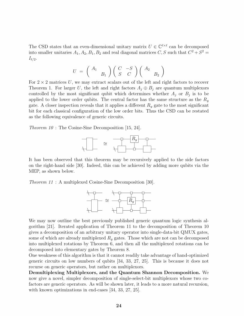
The CSD states that an even-dimensional unitary matrix U ∈ C`×` can be decomposed

into smaller unitaries A1, A2, B1, B2 and real diagonal matrices C, S such that C2+S2 =I`/2.

U =

(

A1B1

)(

C −SS C

)(

A2B2

)

For 2× 2 matrices U , we may extract scalars out of the left and right factors to recoverTheorem 1. For larger U , the left and right factors Aj ⊕ Bj are quantum multiplexorscontrolled by the most significant qubit which determines whether Aj or Bj is to beapplied to the lower order qubits. The central factor has the same structure as the Ry

gate. A closer inspection reveals that it applies a different Ry gate to the most significantbit for each classical configuration of the low order bits. Thus the CSD can be restatedas the following equivalence of generic circuits.

Theorem 10 : The Cosine-Sine Decomposition [15, 24].

∼=Ry

\ \

It has been observed that this theorem may be recursively applied to the side factorson the right-hand side [30]. Indeed, this can be achieved by adding more qubits via theMEP, as shown below.

Theorem 11 : A multiplexed Cosine-Sine Decomposition [30].

\ \

∼= Ry

\ \

We may now outline the best previously published generic quantum logic synthesis al-gorithm [21]. Iterated application of Theorem 11 to the decomposition of Theorem 10gives a decomposition of an arbitrary unitary operator into single-data-bit QMUX gates,some of which are already multiplexed Ry gates. Those which are not can be decomposedinto multiplexed rotations by Theorem 6, and then all the multiplexed rotations can bedecomposed into elementary gates by Theorem 8.One weakness of this algorithm is that it cannot readily take advantage of hand-optimizedgeneric circuits on low numbers of qubits [34, 33, 27, 25]. This is because it does notrecurse on generic operators, but rather on multiplexors.Demultiplexing Multiplexors, and the Quantum Shannon Decomposition. Wenow give a novel, simpler decomposition of single-select-bit multiplexors whose two co-factors are generic operators. As will be shown later, it leads to a more natural recursion,with known optimizations in end-cases [34, 33, 27, 25].

24

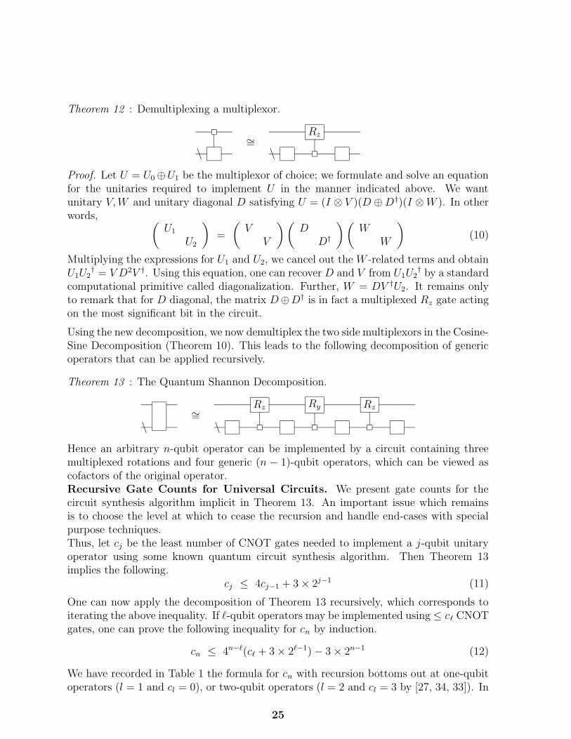
Theorem 12 : Demultiplexing a multiplexor.

∼=Rz

\ \

Proof. Let U = U0⊕U1 be the multiplexor of choice; we formulate and solve an equationfor the unitaries required to implement U in the manner indicated above. We wantunitary V,W and unitary diagonal D satisfying U = (I ⊗ V )(D ⊕D†)(I ⊗W ). In otherwords,

(

U1U2

)

=

(

VV

)(

DD†

)(

WW

)

(10)

Multiplying the expressions for U1 and U2, we cancel out the W -related terms and obtainU1U2

† = V D2V †. Using this equation, one can recover D and V from U1U2† by a standard

computational primitive called diagonalization. Further, W = DV †U2. It remains onlyto remark that for D diagonal, the matrix D⊕D† is in fact a multiplexed Rz gate actingon the most significant bit in the circuit.

Using the new decomposition, we now demultiplex the two side multiplexors in the Cosine-Sine Decomposition (Theorem 10). This leads to the following decomposition of genericoperators that can be applied recursively.

Theorem 13 : The Quantum Shannon Decomposition.

∼=Rz Ry Rz

\ \

Hence an arbitrary n-qubit operator can be implemented by a circuit containing threemultiplexed rotations and four generic (n − 1)-qubit operators, which can be viewed ascofactors of the original operator.Recursive Gate Counts for Universal Circuits. We present gate counts for thecircuit synthesis algorithm implicit in Theorem 13. An important issue which remainsis to choose the level at which to cease the recursion and handle end-cases with specialpurpose techniques.Thus, let cj be the least number of CNOT gates needed to implement a j-qubit unitaryoperator using some known quantum circuit synthesis algorithm. Then Theorem 13implies the following.

cj ≤ 4cj−1 + 3× 2j−1 (11)

One can now apply the decomposition of Theorem 13 recursively, which corresponds toiterating the above inequality. If `-qubit operators may be implemented using ≤ c` CNOTgates, one can prove the following inequality for cn by induction.

cn ≤ 4n−`(c` + 3× 2`−1)− 3× 2n−1 (12)

We have recorded in Table 1 the formula for cn with recursion bottoms out at one-qubitoperators (l = 1 and cl = 0), or two-qubit operators (l = 2 and cl = 3 by [27, 34, 33]). In

25

Number of qubits and gate countsSynthesis Algorithm 1 2 3 4 5 6 7 n

Original QR decomp. [3, 9] ——– O(n34n)Improved QR decomp. [20] ——– O(n4n)Palindrome transform [2] ——– O(n4n)

QR [31, Table I] 0 4 64 536 4156 22618 108760 O(4n)QR (Theorem 9) 0 8 62 344 1642 7244 30606 2× 4n − (2n + 3)× 2n + 2nCSD [21, p. 4] 0 8 48 224 960 3968 16128 4n − 2× 2n

QSD (l = 1) 0 6 36 168 720 2976 12096 (3/4)× 4n − (3/2)× 2n

QSD (l = 2) 0 3 24 120 528 2208 9024 (9/16)× 4n − (3/2)× 2n

QSD (l = 2, optimized) 0 3 20 100 444 1868 7660 (23/48)× 4n − (3/2)× 2n + 4/3

Lower bounds [27] 0 3 14 61 252 1020 4091 d 1

4(4n − 3n− 1)e

Table 1: A comparison of CNOT counts for unitary circuits generated by several algo-rithms (best results are in bold). We have labeled the algorithms by the matrix decom-position they implement. The results of our work are boldfaced, including an optimizedQR decomposition and three algorithms based on the Quantum Shannon Decomposition(QSD).

either case, we improve on the best previously published algorithm in [21]. However, toobtain our advertised CNOT-count of (23/48)× 4n − (3/2)× 2n + 4/3 we shall need twofurther optimizations discussed in our upcoming publication in IEEE Trans. on CAD.Note that for n = 3, only 20 CNOTs are needed. This is the best known three-qubitcircuit at present (a less efficient circuit is given in [32]). Thus, our algorithm is the firstefficient n-qubit circuit synthesis routine which also produces a best-practice circuit in asmall number of qubits.Nearest-Neighbor Circuits. A frequent criticism of quantum logic synthesis (espe-cially highly optimized circuits which nonetheless must conform to large theoretical lowerbounds on the number of gates) is that the resulting circuits are physically impractical.In particular, naıve gate counts ignore many important physical problems which arisein practice. Many such are grouped under the topic of quantum architectures [5, 23],including questions of (1) how best to arrange the qubits and (2) how to adapt a circuitdiagram to a particular physical layout. A spin chain s perhaps the most restrictive archi-tecture: the qubits are laid out in a line, and all CNOT gates must act only on adjacent(nearest-neighbor) qubits. As spin-chains embed into two and three dimensional grids,we view them as the most difficult architecture from the perspective of layout. The workin [14] shows how to adapt Shor’s algorithm to spin-chains without asymptotic increasein gate counts. However, it is not yet clear if generic circuits can be adapted similarly.As shown next, our circuits adapt well to the spin-chain limitations. Most CNOT gatesused in our decomposition already act on nearest neighbors, e.g., those gates implementingthe two-qubit operators. Moreover, Fig. 6 shows that only 2n−k CNOT gates of lengthk (where the length of a local CNOT is 1) will appear in the circuit implementing amultiplexed rotation with (n − 1) control bits. Figure 7 decomposes a length k CNOTinto 4k − 4 length 1 CNOTs. Summation shows that 9 × 2n−1 − 8 nearest-neighborCNOTs suffice to implement the multiplexed rotation. Therefore restricting CNOT gatesto nearest-neighbor interactions increases CNOT count by at most a factor of nine.

26

• • •ÂÁÀ¿»¼½¾ • • ÂÁÀ¿»¼½¾ • •

∼= ÂÁÀ¿»¼½¾ • ÂÁÀ¿»¼½¾ ÂÁÀ¿»¼½¾ • ÂÁÀ¿»¼½¾

ÂÁÀ¿»¼½¾ ÂÁÀ¿»¼½¾ ÂÁÀ¿»¼½¾

Figure 7: Implementing a long-range CNOT gate with nearest-neighbor CNOTs.

Summary and Open Questions. Our approach to quantum circuit synthesis empha-sizes simplicity, a well-pronounced top-down structure, and practical computation via theCosine-Sine Decomposition. By introducing the quantum multiplexor and optimizing itssingly-controlled version, we derived a quantum analogue of the well-known Shannon de-composition of Boolean functions. Applying this decomposition recursively to quantumoperators leads to a circuit synthesis algorithm in terms of quantum multiplexors. Asseen in Table 1, our techniques achieve the best known controlled-not counts, both forsmall numbers of qubits and asymptotically. Our approach has the additional advantagethat it co-opts all results on small numbers of qubits – e.g., future specialty techniquesdeveloped for three-qubit quantum logic synthesis can be used as terminal cases of ourrecursion. We have also discussed various problems specific to quantum computation,specifically initialization of quantum registers and mapping to the nearest-neighbor gatelibrary.

References

[1] The ARDA Roadmap For Quantum Information Science and Technology,http://qist.lanl.gov .

[2] A. V. Aho and K. M. Svore. Compiling quantum circuits using the palindrometransform. e-print, quant-ph/0311008.

[3] A. Barenco, C. Bennett, R. Cleve, D.P. DiVincenzo, N. Margolus, P. Shor, T. Sleator,J.A. Smolin, and H. Weinfurter, Elementary gates for quantum computation. Phys.Rev. A, 52:3457, 1995.

[4] C. H. Bennett and G. Brassard. Quantum cryptography: Public-key distributionand coin tossing. In Proceedings of IEEE International Conference on Computers,Systems, and Signal Processing, page 175179, Bangalore, India, 1984. IEEE Press.

[5] G.K. Brennen, D. Song, and C.J. Williams, Quantum-computer architecture usingnonlocal interactions. Phys. Rev. A.(R), 67:050302, 2003.

27

[6] S.S. Bullock, Note on the Khaneja Glaser decomposition. Quant. Info. and Comp.4:396, 2004.

[7] S. S. Bullock and I. L. Markov. An elementary two-qubit quantum computationin twenty-three elementary gates. In Proceedings of the 40th ACM/IEEE DesignAutomation Conference, pages 324–329, Anaheim, CA, June 2003. Journal: Phys.Rev. A 68:012318, 2003.

[8] S. S. Bullock and I. L. Markov, Smaller circuits for arbitrary n-qubit diagonalcomputations. Quant. Info. and Comp. 4:27, 2004.

[9] G. Cybenko: “Reducing Quantum Computations to Elementary Unitary Opera-tions”, Comp. in Sci. and Engin., March/April 2001, pp. 27-32.

[10] D. Deutsch, Quantum Computational Networks, Proc. R. Soc. London A 425:73,1989.

[11] D. Deutsch, A. Barenco, A. Ekert, Universality in quantum computation. Proc. R.Soc. London A 449:669, 1995.

[12] D. P. DiVincenzo. Two-bit gates are universal for quantum computation. Phys. Rev.A 15:1015, 1995.

[13] R. P. Feynman. Quantum mechanical computers. Found. Phys., 16:507–531, 1986.

[14] A. G. Fowler, S. J. Devitt, L. C. L. Hollenberg, “Implementation of Shor’s Algorithmon a Linear Nearest Neighbour Qubit Array”, Quant. Info. Comput. 4, 237-251(2004).

[15] G.H. Golub and C. vanLoan, Matrix Computations, Johns Hopkins Press, 1989.

[16] L. K. Grover. Quantum mechanics helps with searching for a needle in a haystack.Phys. Rev. Let., 79:325, 1997.

[17] W. N. N. Hung, X. Song, G. Yang, J. Yang, and M. Perkowski. Quantum logicsynthesis by symbolic reachability analysis. In Proceedings of the 41st Design Au-tomation Conference, San Diego, CA, June 2004.

[18] K. Iwama, Y. Kambayashi, and S. Yamashita. Transformation rules for designingcnot-based quantum circuits. In Proceedings of the 39th Design Automation Confer-ence, pages 419–425, 2002.

[19] R. Jozsa and N. Linden, On the role of entanglement in quantum computationalspeed-up. e-print, quant-ph/0201143.

[20] E. Knill, Approximation by quantum circuits. LANL report LAUR-95-2225.

[21] M. Mottonen, J. J. Vartiainen, V. Bergholm, and M. M. Salomaa. Quantum circuitsfor general multiqubit gates. Phys. Rev. Let., 93:130502, 2004.

28

[22] M. A. Nielsen and I. L. Chuang. Quantum Computation and Quantum Information.Cambridge University Press, 2000.

[23] M. Oskin, F.T. Chong, I. Chuang, and J. Kubiatowicz, Building quantum wires:the long and the short of it. In 30th Annual International Symposium on ComputerArchitecture (ISCA), June 2003.

[24] C. C. Paige and M. Wei. History and generality of the CS decomposition. LinearAlg. and App., 208:303, 1994.

[25] V. V. Shende, S. S. Bullock, and I. L. Markov. Recognizing small-circuit structurein two-qubit operators. Phys. Rev. A, 70:012310, 2004.

[26] V. V. Shende and I. L. Markov. Quantum Circuits for Incompletely Specified Two-Qubit Operators Quant. Inf. and Comput., vol.5, no.1, pp. 49-58, January 2005.

[27] V. V. Shende, I. L. Markov, and S. S. Bullock. Smaller two-qubit circuits for quantumcommunication and computation. In Design, Automation, and Test in Europe, pages980–985, Paris, France, February 2004. Journal: Phys. Rev. A, 69:062321, 2004.

[28] V. V. Shende, A. K. Prasad, I. L. Markov, and J. P. Hayes. Synthesis of reversiblelogic circuits. IEEE Transactions on Computer Aided Design, 22:710, 2003.

[29] P. Shor. Polynomial-time algorithms for prime factorization and discrete logarithmon a quantum computer. SIAM Journal on Computing, 26(5):1484–1509, 1997.

[30] R. R. Tucci, A Rudimentary Quantum Compiler. e-print, quant-ph/9805015.

[31] J. J. Vartiainen, M. Mottonen, and M. M. Salomaa. Efficient decomposition ofquantum gates. Phys. Rev. Let., 92:177902, 2004.

[32] F. Vatan and C. Williams. Realization of a general three-qubit quantum gate. e-print, quant-ph/0401178.

[33] F. Vatan and C. Williams. Optimal quantum circuits for general two-qubit gates.Phys. Rev. A, 69:032315, 2004.

[34] G. Vidal and C. M. Dawson. A universal quantum circuit for two-qubit transforma-tions with three CNOT gates. Phys. Rev. A, 69:010301, 2004.

[35] J. Zhang, J. Vala, S. Sastry, and K. B. Whaley. Exact two-qubit universal quantumcircuit. Phys. Rev. Let., 91:027903, 2003.

[36] V. V. Zhirnov, R. K. Cavin, J. A. Hutchby, and G. I. Bourianoff. Limits to binarylogic switch scaling — a gedanken model. Proceedings of the IEEE, 91(11):1934–1939,November 2003.

29

30

4. Simulation of Quantum Circuits We have developed a novel and practical software means of simulating quantum computers efficiently on classical computers using the state vector representation [13 - 17]. It is based on a new data structure called the Quantum Information Decision Diagram or QuIDD, which uses decision diagram concepts that are well-known in the context of simulating classical computer hardware [1, 6, 7]. We have demonstrated that QuIDDs allow simulations of n-qubit systems to achieve run-time and memory complexities that range from O(1) to O(poly(n)2n), and the worst case is not typical. In the important case of Grover's quantum search algorithm [9], we have shown that our QuIDD-based simulator outperforms all other known simulation techniques. QuIDD Theory. QuIDDs arose from our observation that vectors and matrices encountered in quantum computing contain repeated structures. Complex operators obtained from the tensor product of simpler matrices continue to exhibit common substructures which certain BDD variants can capture. The classical decision diagram structures MTBDDs and ADDs are particularly relevant to the task of simulating quantum systems. The QuIDD can be viewed as an ADD or MTBDD with the following properties:

1. The values of terminal nodes are restricted to the set of complex numbers.

2. Rather than contain the values explicitly, QuIDD terminal nodes contain integer indices that map into a separate array of complex numbers. This allows the use of a simpler integer function for Apply-based operations, along with existing ADD and MTBDD libraries, greatly reducing implementation overhead.

3. The variable ordering of QuIDDs interleaves row and column variables, which favors compression of block patterns.

4. ADDs are usually padded with 0's to represent arbitrarily sized matrices. No such padding is necessary in the quantum domain where all vectors and matrices have sizes that are a power of 2.

As we demonstrate using our QuIDD-based simulator QuIDDPro, these properties greatly enhance performance of quantum computational simulation.

Figure 8 shows the QuIDD structure for three 2-qubit states. We treat the indices of the four vector elements as binary numbers, and define their bits as QuIDD decision variables; a similar definition is used for ADDs. For example, traversing the then edge (solid line) of node I0 in Figure 8c is equivalent to assigning the value 1 to the first bit of the 2-bit vector index. Traversing the else edge (dotted line) of node I1 in the same figure is equivalent to assigning the value 0 to the second bit of the index. These traversals bring us to the terminal value -1/2, which is precisely the value at index 10 in the vector representation.

31

Figure 8: Sample QuIDDs for state vectors of (a) best, (b) worst and (c) mid-range size.

QuIDD representations of matrices extend those of vectors by adding a second type of variable node; they enjoy the same reduction rules and compression benefits. Consider the 2-qubit Hadamard matrix annotated with binary row and column indices shown in Figure 9a. In this case there are two sets of indices, the first (vertical) set corresponds to the rows of the matrix, while the second (horizontal) set corresponds to the columns. We assign the variable names Ri and Cj to the row and column index variables respectively. Figure 9b shows the QuIDD form of this sample matrix where it is used to modify the state vector |00= (1,0,0,0) via matrix-vector multiplication.

Figure 9: (a) A 2-qubit Hadamard matrix and (b) its QuIDD multiplied by |00 =(1,0,0,0). The top-down ordering of the decision variables can drastically affect the level of compression achieved in BDD-based structures such as QuIDDs. The University of Colorado Decision Diagram (CUDD) programming library, which is incorporated into QuIDDPro, has sophisticated dynamic variable-reordering techniques that

32

achieve performance improvements in BDD applications. However, dynamic variable reordering has significant time overhead, so finding a good static ordering in advance may be preferable in some cases. Variable orderings are highly dependent upon the structure of the problem at hand, so one way to obtain a good ordering is to study the problem domain. In the case of quantum computing, we notice that all matrices and vectors contain 2n elements where n is the number of qubits represented. Additionally, the matrices are square and non-singular. Interleaving implies the following variable ordering: R0 < C0 < R1 < C1 < ... < Rn < Cn. Intuitively, the interleaved ordering causes compression to favor regularity in block sub-structures of the matrices. Such regularity is created by tensor products that are required to allow multiple quantum gates to operate in parallel and also to extend smaller quantum gates to operate on larger numbers of qubits. The tensor product A ⊗ B multiplies each element of A by the whole matrix B to create a larger matrix; thus, by definition, the tensor product will propagate block patterns in its operands. To illustrate the notion of block patterns and how QuIDDs take advantage of them, consider the tensor product of two 1-qubit Hadamard operators:

The matrices have been separated into quadrants, and each quadrant represents a block. For the Hadamard matrices depicted, three of the four blocks are equal in both of the one-qubit matrices and also in the larger two-qubit matrix (the equivalent blocks in parentheses). This repetition of equivalent blocks demonstrates that the tensor product of two equal matrices propagates block patterns. In this example, the pattern lies in the fact that all but the lower-right quadrant of an n-qubit Hadamard operator are equal. Furthermore, the structure of the two-qubit matrix implies a recursive block sub-structure, which can be seen by recursively partitioning each of the quadrants in the two-qubit matrix thus:

The only difference between the values in the two-qubit matrix and the values in the one-qubit matrices is a factor of 1/√2. Thus, we can recursively define the Hadamard operator as follows:

−=⊗

−−

−−

−−11

11

11

21

21

21

21

nn

nn

nn

HH

HHHH

Other operators constructed via the tensor product can be defined recursively in a similar fashion. Since three of the four blocks in the n-qubit Hadamard operator are the same, significant redundancy is present for QuIDDs to exploit. The interleaved variable ordering property allows a QuIDD to explicitly represent only two distinct blocks rather than four. As we demonstrate later,

33

compression of equivalent block sub-structures using QuIDDs offers major performance improvements for many of the operators that are frequently used in quantum computation. QuIDD Operations. With the structure and variable ordering in place, operations involving QuIDDs can now be defined. Most operations defined for ADDs also work on QuIDDs with some modification to accommodate the QuIDD properties. Here we describe an algorithm for the tensor product of QuIDDs based on the Apply operation. In general, the tensor product A ⊗ B produces a new matrix which multiplies each element of A by the entire matrix B. Hence rows (columns) of the tensor product matrix are component-wise products of rows (columns) of the argument matrices. Therefore it is straightforward to implement the tensor product operation on QuIDDs using the Apply function with an argument that directs Apply to multiply when it reaches the terminals of both operands. The main difficulty here lies in ensuring that the terminals of A are each multiplied by all the terminals of B. From the definition of the standard recursive Apply routine, we know that variables which precede other variables in the ordering are expanded first. Therefore, we must first shift all variables in B in the current order after all of the variables in A prior to the call to Apply. After this shift is performed, the Apply routine will then produce the desired behavior. Apply starts out with A * B and expands A alone until Aterminal * B is reached for each terminal in A. Once a terminal of A is reached, B is fully expanded, implying that each terminal of A is multiplied by all of B. The size of the resulting QuIDD and the runtime for generating it given two operands of sizes a and b (measured by the number of nodes) is O(ab), because the tensor product simply involves a variable shift of complexity O(b) followed by a call to Apply, which have time and memory complexity O(ab). Matrix multiplication can be implemented very efficiently by using Apply to implement the dot-product operation. This follows from the observation that multiplication is a series of dot-products between the rows of one operand and the columns of the other operand. One call to Apply will not suffice because the dot-product requires two binary operations to be performed, addition and multiplication. To implement this, we simply use the matrix multiplication algorithm previously defined for ADDs [1] but modified to support the QuIDD properties. The algorithm makes two calls to Apply, one for multiplication and the other for addition. Another important issue in efficient matrix multiplication is compression. To avoid the problem that MATLAB encounters with its “packed” representation, ADDs do not require decompression during matrix multiplication. Bahar et al. address this by tracking the number i of skipped variables between the parent node and its child node in each recursive call. Their pseudo-code suggests time-complexity O((ab)2) where a and b are the sizes, i.e., the number of decision nodes, of two ADD operands. As with all BDD algorithms based on the Apply function, the size of the resulting ADD is on the order of the time complexity, meaning that the size is also O((ab)2). In the context of QuIDDs, we use a modified form of this algorithm to multiply operators by the state vector, meaning that a and b will be the sizes in nodes of a QuIDD matrix and QuIDD state vector, respectively. If either a or b or both are exponential in the number of qubits in the circuit, the QuIDD approach will have exponential time and memory complexity. However, many of the operators which arise in quantum computing have QuIDD representations that are polynomial in the number of qubits.

34

Two important modifications must be made to the ADD matrix multiply algorithm in order to adapt it for QuIDDs. To satisfy QuIDD properties 1 and 2, the algorithm must treat the terminals as indices into an array rather than the actual values to be multiplied and added. Also, a variable ordering problem must be accounted for when multiplying a matrix by a vector. A QuIDD matrix is composed of interleaved row and column variables, whereas a QuIDD vector only depends on column variables. If the ADD algorithm is run as described above without modification, the resulting QuIDD vector will be composed of row instead of column variables. The structure will be correct, but the dependence on row variables prevents the QuIDD vector from being used in future multiplications. Thus, we introduce a simple extension which transposes the row variables in the new QuIDD vector to corresponding column variables. In other words, for each Ri variable that exists in the QuIDD vector’s support, we map that variable to Ci. We briefly consider some other linear-algebraic operations. Matrix addition is easily implemented by calling Apply with op defined to be addition. Unlike the tensor product, no special variable order shifting is required for matrix addition. Another interesting operation which is nearly identical to matrix addition is element-wise multiplication cij = aijbij. Unlike the dot-product, this operation involves products and no summation. It is implemented like matrix addition except that op is defined to be multiplication rather than addition. In quantum computer simulation, this operation is useful for matrix-vector multiplications with a diagonal matrix like the conditional phase shift in Grover’s search algorithm. Such a shortcut considerably improves upon full-fledged matrix multiplication. Interestingly, the element-wise multiplication and matrix addition operations for QuIDDs can perform, without the loss of efficiency, the corresponding scalar operations. That is because a QuIDD with a single terminal node can be viewed both as a scalar value and as a matrix or vector with repeated values. Since matrix addition, element-wise multiplication, and their scalar counterparts are nothing more than calls to Apply, the runtime complexity of each operation is O(ab) where a and b are the sizes in nodes of the QuIDD operands. Likewise, the resulting QuIDD has memory complexity O(ab). Another very relevant operation on QuIDDs is the transpose. It is perhaps the simplest QuIDD operation because it is accomplished by swapping the row and column variables. The transpose is easily extended to the complex conjugate transpose (also known as the Hermitian conjugate or adjoint) by first obtaining the transpose of a QuIDD and then conjugating its terminal values. The runtime and memory complexity of these operations is O(a) where a is the size in nodes of the target QuIDD. To perform quantum measurement, one can use the inner product, which is often faster than multiplying by projection matrices and computing norms. The inner product BA of two QuIDD vectors is computed by matrix multiplying the transpose of A with B. Since matrix multiplication is involved, the runtime and memory complexity of the inner product is O((ab)2), where a and b are the sizes in nodes of A and B respectively. QuIDDPro currently supports matrix multiplication, the tensor product, measurement, matrix addition, element-wise multiplication, scalar operations, the transpose, the complex conjugate transpose, and the inner product. Measurement is defined using a combination of QuIDD operations. After measurement, the state vector is described by

35

Here Mm is the measurement operator; it can be represented by a QuIDD matrix, and the state vector Ψ can be represented by a QuIDD vector. The expression in the numerator involves a

QuIDD matrix multiplication. In the denominator, !mM is the complex conjugate transpose of Mm,

which is also defined for QuIDDs, and ΨΨ mm MM ! is an inner product which produces a

QuIDD with a single terminal node. Taking the square root of the value in this terminal node is straightforward. To complete the measurement operation, scalar division is performed with the QuIDD in the numerator and the single terminal QuIDD in the denominator as operands. Let a and b be the sizes in nodes of the measurement operator QuIDD and state vector QuIDD, respectively. Performing the matrix multiplication in the numerator has runtime and memory complexity O((ab)2). The scalar division between the numerator and denominator has the same runtime and memory complexity since the denominator is a QuIDD with a single terminal node. However, computing the denominator will have runtime and memory complexity O(a16b6) due to the matrix-vector multiplications and inner product. Complexity Analysis. Next we show that the QuIDD data structure can represent a large class of state vectors and operators using an amount of memory that is linear in the number of qubits rather than exponential. Further, we show that the main QuIDD operations required in quantum circuit simulation, i.e., matrix multiplication, the tensor product, and measurement, have both runtime and memory that is linear in the number of qubits for the same class of state vectors and operators. We also analyze the runtime and memory complexity of simulating Grover's algorithm using QuIDDs.

Figure 10: General form of a tensor product between two QuIDDs A and B.

36

The key to analyzing the runtime and memory complexity of the QuIDD-based simulations lies in the mechanics of the tensor product. In the following analysis, the size of a QuIDD is represented by the number of nodes rather than the actual memory space used. Since the amount of memory used by a single QuIDD node is a constant, size in nodes is relevant for asymptotic complexity arguments. Actual memory usage in megabytes of QuIDD simulations is reported later. Figure 10 illustrates the general form of a tensor product between two QuIDDs A and B. In(A) represents the internal nodes of A, while a1 through ax denote terminal nodes. The notation for B is similar. In(A) is the root subgraph of the tensor product result because of the interleaved variable ordering defined for QuIDDs and the variable shifting operation of the tensor product. Suppose that A depends on the variables R0 < C0 < ... < Ri < Ci, and B depends on the variables R0 < C0 < ... < Rj < Cj. In computing A ⊗ B, the variables on which B depends will be shifted to Ri+1 < Ci+1 < ... < Rk+i+1 < C k+i+1. The tensor product is then completed by calling Apply(A, B, *). Due to the variable shift on B, Rule 1 of the Apply function is used after each comparison of a node from A with a node from B until the terminals of A are reached. Using Rule 1 for each of these comparisons implies that only nodes from A will be added to the result, explaining the presence of In(A). Once the terminals of A are reached, Rule 2 of Apply is invoked since terminals are defined to appear last in the variable ordering. Using Rule 2 when the terminals of A are reached implies that all the internal nodes from B are added in place of each terminal of A, causing x copies of In(B) to appear in the result (recall that there are x terminals in A). When the terminals of B are reached, they are multiplied by the appropriate terminals of A. Specifically, the terminals of a copy of B will each be multiplied by the terminal of A that its In(B) replaced. The same reasoning holds for QuIDD vectors as vectors differ in that they depend only on Ri variables. Figure 10 suggests that the size of a QuIDD constructed via the tensor product depends on the number of terminals in the operands. The more terminals a left-hand tensor operand contains, the more copies of the right-hand tensor operand’s internal nodes will be added to the result. More formally, consider the tensor product of a series of QuIDDs:

)))((( 3211 nini QQQQQ ⊗⊗⊗⊗=⊗ =

The ⊗ operation is associative so parentheses do not affect the result, but it is not commutative. If the number of terminals in i

ni Q1=⊗ increases by a certain factor with each Qi, then i

ni Q1=⊗ must

grow exponentially in n. If, however, the number of terminals stops changing, then ini Q1=⊗ grows

linearly in n. Thus, the growth depends on the matrix entries because terminals of A ⊗ B are products of terminal values of A by terminal values of B, and repeated products are merged. If all QuIDDs Qi’s have terminal values from the same set Γ, the product's terminal values are products of elements from Γ. Consider finite non-empty sets of complex numbers Γ1 and Γ2, and define their all-pairs product as xy | x ∈ Γ1, y ∈ Γ2. One can verify that this operation is associative, and therefore the set Γn of all n-element products is well defined for n > 0. We then call a finite non-empty set Γ ⊂ C persistent iff the size of Γn is constant for all n > 0. For example, the set Γ = c,-c is persistent for any c because Γn = cn,-cn. In general, any set closed under multiplication is persistent, but that is not a necessary condition. An important example of a persistent set is the set consisting of 0 and all n-th degree roots of unity Un= e2πik/n | k = 0...n - 1, for some n. Since roots of unity form a

37

group, they are closed under multiplication and form a persistent set. The importance of persistent sets is underlined by the following result. Theorem 14: Given a persistent set Γ and a constant C, consider n QuIDDs with at most C nodes each and terminal values from a persistent set Γ. The tensor product of those QuIDDs has O(n) nodes and can be computed in O(n) time.

Importantly, the terminal values do not need to form a persistent set themselves for the theorem to hold. If they are contained in a persistent set, then the sets of all possible m-element products (i.e. m < n for all n-element products in a set Γ) eventually stabilize in the sense that their sizes do not exceed that of Γ. However, this is only true for a fixed m rather than for the sets of products of m and fewer elements. Theorem 15: Consider measuring an n-qubit QuIDD state vector Ψ using a QuIDD measurement

operator M, where both Ψ and M are constructed via the tensor product of an arbitrary sequence of O(1)-sized QuIDD vectors and matrices, respectively. If the terminal node values of the O(1)-sized QuIDD vectors or operators are in a persistent set Γ, then the runtime and memory complexity of measuring the QuIDD state vector is O(n22). The class of QuIDDs described by Theorem 15 above encompasses a large number of practical quantum state vectors and operators. These include, but are not limited to, any equal superposition of n qubits, any sequence of n qubits in the computational basis states, n-qubit Pauli matrices, and n-qubit Hadamard matrices. These results suggest a polynomial-sized QuIDD representation of any quantum circuit on n qubits in terms of such gates if the number of gates is limited by a constant. In other words, the above sufficient conditions apply if the depth (length) of the circuit is limited by a constant. Our simulation technique may use polynomial memory and runtime in other circumstances as well, as shown next. Grover’s Algorithm. To investigate the power of the QuIDD representation, we used QuIDDPro to simulate Grover’s algorithm, one of the two major quantum algorithms developed to date [9]. Grover’s algorithm searches for a subset of items in an unordered database of N items. The only selection criterion available is a black-box predicate that can be evaluated on any item in the database. The complexity of this evaluation (query) is unknown, and the overall complexity analysis is performed in terms of queries. In the classical domain, any algorithm for such an unordered search must query the predicate Ω(N) times. However, Grover’s algorithm can perform the search with quantum query complexity O(√N), a quadratic improvement. This assumes that a quantum version of the search predicate can be evaluated on a superposition of all database items. A quantum circuit representation of the algorithm involves five major components: an oracle circuit, a conditional phase shift operator, sets of Hadamard gates, the data qubits, and an oracle qubit. The oracle circuit is a Boolean predicate that acts as a filter, flipping the oracle qubit when it receives as input an n bit sequence representing the items being searched for. In quantum circuit form, the oracle is represented as a series of controlled NOT gates with subsets of the data qubits acting as the control qubits and the oracle qubit receiving the action of the NOT gates. Following the oracle circuit, Hadamard gates put the n data qubits into an equal superposition of all 2n items

38

in the database where 2n = N. Then a sequence of gates 11 −⊗−⊗ nn CHH , where C denotes the conditional phase shift operator, are applied iteratively to the data qubits. Each iteration is termed a Grover iteration. Grover’s algorithm must be stopped after a certain number of iterations when the probability amplitudes of the states representing the items sought are sufficiently boosted. There must be enough iterations to ensure a successful measurement, but after a certain point the probability of successful measurement starts fading, and later changes periodically. In our experiments, we used the tight bound on the number of iterations formulated by Boyer et al. [5], when the number of solutions M is known in advance to be θπ 4/ where NM /=θ . The power of Grover’s algorithm lies in the fact that the data qubits store all N items in the database as a superposition, allowing the oracle circuit to find all items being searched for simultaneously. A circuit implementing Grover's algorithm is shown in Figure 11.

Figure 11: Circuit-level implementation of Grover’s algorithm. The target algorithm can be summarized as follows, where N denotes the number of elements in the database. 1. Initialize n qubits to |0 and the oracle qubit to |1 .2. Apply the Hadamard transform to all qubits to put them in a uniform superposition of basis states. 3. Apply the oracle circuit, this can be implemented as a series of one or more CNOT gates representing the search criteria. The inputs to the oracle circuit feed the control parts of the CNOT gates, while the oracle qubit is the target qubit for all the CNOTs. If the input to this circuit satisfies the search criteria, the oracle qubit is flipped. For a superposition of inputs, those input basis states that satisfy the search criteria flip the oracle qubit in the composite state-space. The

39

oracle circuit uses ancillary qubits as its workspace, reversibly returning them to their original states (shown as |0 in Figure 11). 4. Apply the H gate to all qubits except the oracle qubit. 5. Apply the conditional phase-shift gate on all qubits except the oracle qubit. This operation negates the probability amplitude of the |000... 0 basis state, leaving that of the others unaffected. It can be realized using a combination of X, H and Cn-1-NOT gates as shown. A decomposition of the Cn-1-NOT into elementary gates is given in [2]. 6. Apply the H gate to all gates except the oracle qubit. 7. Repeat steps 3-6 (a single Grover iteration) R =

MN

4π

times, where M is the number of keys

matching the search criteria. 8. Apply the H gate to the oracle qubit in the last iteration. Measure the first n qubits to obtain the index of the matching key with high probability. Using explicit vectors and matrices to simulate the above procedure would incur memory and runtime complexities of Ω(N). However, this is not necessarily the case when using QuIDDs. To show this, we give a step-by-step complexity analysis for a QuIDD-based simulation of the procedure. Steps 1 and 2: Theorem 15 implies that the memory and runtime complexity of step 1 is O(n). Step 2 is simply a matrix multiplication of an n-qubit Hadamard matrix with the state vector constructed in step 1. The Hadamard matrix has memory complexity O(n) by the theorem. Since the state vector also has memory complexity O(n), further matrix-vector multiplication in step 2 has O(n4) memory and runtime complexity because computing the product of two QuIDDs A and B takes O((|A||B|)2) time and memory [1]. This upper-bound can be trivially tightened, however. The function of these steps is to put the qubits into an equal superposition. For the n data qubits, this produces a QuIDD with O(1) nodes because an n-qubit state vector representing an equal superposition has only one distinct element, namely 1/2n/2. Also, applying a Hadamard matrix to the single oracle qubit results in a QuIDD with O(1) nodes because in the worst-case, the size of a 1-qubit QuIDD is clearly a constant. Since the tensor product is based on the Apply algorithm, the result of tensoring the QuIDD representing the data qubits in an equal superposition with the QuIDD for the oracle qubit is a QuIDD containing O(1) nodes. Steps 3-6: In step 3, the state vector is matrix-multiplied by the oracle matrix. Again, the complexity of multiplying two arbitrary QuIDDs A and B is O((|A||B|)2). The size of the state vector in step 3 is O(1). If the size of the oracle is |A|, then the memory and runtime complexity of step 3 is O(|A|2). Similarly, steps 4, 5 and 6 have polynomial memory and runtime complexity in terms of |A| and n. (As noted in step 5, the conditional phase-shift operator can be decomposed into the tensor product of single qubit matrices, giving it memory complexity O(n).) Thus we arrive at the O(|A|16n14) worst-case upper-bound for the memory and runtime complexity of the simulation at step 6. Our empirical data suggests that this bound is typically very loose and pessimistic. Step 7: This step does not involve a quantum operator; rather it repeats a Grover iteration R =

MN

4π times. As a result, step 7 induces an exponential runtime for the simulation, since the

40

number of Grover iterations is a function of N = 2n. This is acceptable though because an actual quantum computer would also require exponentially many Grover iterations in order to measure one of the matching keys with a high probability. Ultimately, this is the reason why Grover’s algorithm only offers a quadratic and not an exponential speedup over classical search. Since we showed that the memory and runtime complexity of a single Grover iteration is polynomial in the size of the oracle QuIDD, one might guess that the memory complexity of step 7 is exponential like the runtime. However, it turns out that the size of the state vector does not change from iteration to iteration, as shown below. We now state without proof a few useful properties of QuIDDs. The internal nodes of the state vector QuIDD at the end of any Grover iteration i are equal in number to the internal nodes of the state vector QuIDD at the end of iteration i + 1. Also the total number of nodes in the state vector QuIDD at the end of iteration i is equal to the total number of nodes in the state vector QuIDD at the end of iteration i + 1. Consequently, in a QuIDD-based simulation the runtime and memory complexity of any Grover iteration i is equal to the runtime and memory complexity of iteration i + 1. This means that step 7 does not necessarily induce memory complexity that is exponential in the number of qubits. This important fact is captured in the following theorem. Theorem 16: The memory complexity of simulating Grover’s algorithm using QuIDDs is polynomial in the size of the oracle QuIDD and the number of qubits. Here we do not account for the resources required to construct the QuIDD of the oracle. The overall memory complexity of simulating Grover’s algorithm with QuIDDs is O(|A|16n14), where A is the number of nodes in the oracle QuIDD and n is the number of qubits. While any polynomial-time quantum computation can be simulated in polynomial space, the commonly-used linear-algebraic simulation requires Ω(2n) space. Note that the case of an oracle searching for a unique solution (as originally considered by Grover) implies that |A| = n. Here most of the searching will be done while constructing the QuIDD of the oracle, which is an entirely classical operation. As we demonstrate experimentally below, for some oracles, simulating Grover’s algorithm with QuIDDs has memory complexity O(n). Furthermore, simulation using QuIDDs has worst-case runtime complexity O(R|A|16n14), where R is the number of Grover iterations as defined earlier. If A grows polynomially with n, this runtime complexity is the same as that of an ideal quantum computer up to a polynomial factor. Empirical Validation: Next we discuss problems that arise when implementing a QuIDD-based simulator. We also present experimental results obtained from actual simulation. Full support of QuIDDs requires the use of complex arithmetic, which can lead to serious problems if numerical precision is not adequately addressed. At an abstract level, ADDs can support terminals of any numerical type, but CUDD’s implementation of ADDs does not. For efficiency reasons, CUDD stores node information in C “unions,” which are interpreted numerically for terminals and as child pointers for internal nodes. However, it is well-known that unions are incompatible with the use of C++ classes because their multiple interpretations hinder

41

the binding of correct destructors. In particular, complex numbers in C++ are implemented as a templated class and are incompatible with CUDD. This was one of the motivations for storing terminal values in an external array. Another important practical issue is the precision of complex numeric types. Over the course of repeated multiplications, the values of some terminals may become very small and induce round-off errors if the standard IEEE double-precision floating-point types are used. This effect worsens for larger circuits. Such round-off errors can significantly affect the structure of a QuIDD by merging terminals that are only slightly different, or not merging terminals whose values should be equal, but differ by a small computational error. The use of approximate comparisons with an epsilon works in certain cases but does not scale well, particularly for creating an equal superposition of states, a standard operation in quantum circuits. In an equal superposition, a circuit with n qubits will contain the terminal value 1/2n/2 in the state vector. With the IEEE double-precision floating-point type, this value will be rounded to zero at n = 2048, preventing the use of epsilons for approximate comparison past n = 2048. Furthermore, a static value of epsilon will not work well for different sized circuits. For example, ε = 10-6 may work well for n = 35 but not for n = 40, because at 40 all values may be less than 10-6. Therefore, to address the numerical problem, QuIDDPro uses an arbitrary precision floating-point type from the GMP library with the C++ complex template. Precision is then limited only by the available amount of memory in the system. Finally, we present the results for an extensive set of experiments using QuIDDPro to simulate Grover’s Algorithm. Before starting simulation of an instance of the algorithm, we construct the QuIDD representations of Hadamard operators by incrementally tensoring together 1-qubit versions of their matrices n - 1 times to get n-qubit versions. All other QuIDD operators are constructed similarly. Table2 shows sizes (in nodes) of respective QuIDDs at n qubits, where n = 20...100. We observe that memory usage grows linearly in n, and as a result QuIDD-based simulations of Grover’s algorithm are not memory-limited even at 100 qubits. Observe that this is consistent with Theorem 16.

Table 2: Size of QuIDDs (number of nodes) for Grover’s algorithm.

42

Table 3: Simulating Grover's algorithm with n qubits using Octave (Oct), MATLAB (MAT), Blitz++ (B++) and QuIDDPro (QP) with Oracle Design 1. With the operators constructed, simulation can proceed. Tables 3 and 4 compare QuIDDPro (QP) against qubit-wise implementations of Grover’s algorithm using MATLAB, Blitz++ (a high-performance numerical linear algebra library for C++), Octave (a mathematical package similar to MATLAB), and QuIDDPro using two different oracle types. Here “>24hrs” indicates that the runtime exceeded 24 hours, and “>1.5 GB” indicates that memory usage exceeded 1.5GB. Simulation runs that exceed the memory cutoff can also exceed the time cutoff, though we give memory cutoff precedence. NA indicates that after a cutoff of one week, the memory usage was still steadily growing, preventing a peak memory usage measurement. Results were produced on a 1.2GHz AMD Athlon with 2GB RAM running Linux. Memory usage for MATLAB and Octave is lower-bounded by the size of the state vector and conditional phase shift operator; Blitz++ and QuIDDPro memory usage is measured as the size of the entire program. Simulations using MATLAB and Octave past 15 qubits timed out at 24 hours. Table 3 shows performance measurements for simulating Grover's algorithm with an oracle circuit that searches for one item out of 2n. It can be seen that QuIDDPro achieves asymptotic memory savings compared to Blitz++, MATLAB and Octave. The overall runtimes are still exponential in

43

n because Grover’s algorithm entails an exponential number of iterations, even on an actual quantum computer. We also studied a “mod-1024” oracle circuit that searches for elements whose ten least significant bits are 1 (Table 4).

Table 4: Simulating Grover's algorithm with n qubits using Octave (Oct), MATLAB (MAT), Blitz++ (B++) and QuIDDPro (QP) with Oracle Design 2. To verify that the QuIDDPro simulation resulted in the exact number of Grover iterations required to generate the highest probability of measuring the items being sought as per the Boyer et al. formula, we tracked the probabilities of these items as a function of the number of iterations. For this experiment, we used four different oracle circuits, each with 11, 12 and 13 qubit circuits. The first oracle is called Oracle N' and represents an oracle in which all the data qubits act as controls to flip the oracle qubit. The other oracle circuits are Oracle N - 1, Oracle N - 2, and Oracle N - 3, which all have the same structure as Oracle N minus 1, 2 and 3 controls, respectively. As described earlier, each removal of a control doubles the number of items being searched for in the database. For example, Oracle N - 2 searches for 4 items in the data set because it recognizes the bit pattern 111...1dd.

44

Table 5: Number of Grover iterations at which [5] predict the highest

probability of measuring one of the items sought. Table 5 shows the optimal number of iterations produced with the Boyer et al. formulation for all the instances tested. Figure 12 plots the probability of successfully finding any of the items sought against the number of Grover iterations. In the case of Oracle N, we plot the probability of measuring the single item being searched for. Similarly, for Oracles N - 1, N - 2, and N - 3, we plot the probability of measuring any one of the 2, 4 and 8 items being searched for, respectively. By comparing the results in Table 5 with those in Figure 12 it can be easily verified that QuIDDPro uses the correct number of iterations at which measurement is most likely to produce items sought. Also notice that the probabilities, as a function of the number of iterations, follow a sinusoidal curve. It is therefore important to terminate at the exact optimal number of iterations not only from an efficiency standpoint but also to prevent the probability amplitudes of the items being sought from lowering back down toward 0.

Figure 12: Probability of successful search for one, two, four and eight items as a function of the number of iterations after which the measurement is performed. In summary, we have proposed and tested a new technique for simulating quantum circuits using a data structure called a QuIDD. We have shown that QuIDDs enable practical, generic and reasonably efficient simulation of quantum computation. Their key advantages are faster

45

execution and lower memory usage. In our experiments, QuIDDPro achieves exponential memory savings compared to other known techniques. This result is a useful contribution to ongoing research that explores the limitations of quantum computing. Classical computers have the advantage that they are not subject to quantum measurement and errors. Thus, when competing with quantum computers, classical computers can run ideal error-free quantum algorithms, allowing techniques such as QuIDDs to exploit the symmetries found in ideal quantum computation. On the other hand, quantum computation still has certain operators which cannot be represented using only polynomial resources on a classical computer, even with QuIDDs. Examples of such operators include the quantum Fourier Transform and its inverse, which are used in Shor’s number factoring algorithm. Since N = 2n where n is the number of qubits, QuIDDs for the quantum Fourier transform will exhibit exponential growth with a linear increase in qubits. Therefore, the Fourier transform will cause QuIDDPro to have exponential runtime and memory requirements when simulating Shor’s algorithm.

Density Matrix Simulation. We have extended our QuIDD-based quantum circuit simulation to handle the density matrix representation [13]. As noted earlier, density matrices are crucial in capturing interactions between quantum states and the environment, such as noise. In addition to the standard set of operations required to simulate with the state-vector model, including matrix multiplication and the tensor product, simulation with the density matrix model requires the outer product and the partial trace. The outer product is used in the initialization of qubit density matrices, while the partial trace allows a simulator to differentiate qubit states coupled to noisy environments or other unwanted states. The partial trace is invaluable in error modeling since it facilitates descriptions of single qubit states that have been affected by noise and other phenomena [11]. As a result, this work presents algorithms which implement the outer product and the partial trace using QuIDDs.

We also describe a set of quantum circuit benchmarks that incorporate errors, error correction, reversible logic, quantum communication, and quantum search. To empirically evaluate the improvements offered by QuIDD-based density matrix simulation, we use these benchmarks to compare QuIDDPro with an optimized array-based density matrix simulator called QCSim [4]. Performance data from both simulators show that our new graph-based algorithms far outperform the array-based approach for the given benchmarks. It should be noted, however, that not all quantum circuits can be simulated efficiently with QuIDDs. A useful class of matrices and vectors which can be manipulated efficiently by QuIDDs was formally described in the previous section and is restated below. For some matrices and vectors outside of this class, QuIDD-based simulation can be up to three times slower due to the overhead of following pointers in the QuIDD datastructure.

Although the density matrix representation can be invaluable for simulating environmental noise in quantum circuits, like the state vector representation, it is plagued by a simulation complexity that grows exponentially with the number of qubits in the worst case. A straightforward linear-algebraic simulation using density matrices requires O(22n) time and memory resources. Since QuIDDs have proven useful in reducing this complexity in the state vector paradigm, it is only natural to extend QuIDDs to the density matrix model in an attempt to reduce the simulation

46

complexity of this important model in practical cases. Before proceeding to the new extensions, we first review what is already in place that can be re-used in the density matrix representation.

Figure 13: (a) QuIDD for the density matrix resulting from U|01 01|U!, where U = H ⊗ H, and (b) its explicit matrix form.

Figure 13a shows the QuIDD that results from applying U to an outer product as U|01 01|U!, where U = H ⊗ H. The Ri nodes of the QuIDD encode the binary indices of the rows in the explicit matrix. Similarly, the Ci nodes encode the binary indices of the columns. Solid lines leaving a node denote the positive cofactor of the index bit variable (a value of 1), while dashed lines denote the negative cofactor (a value of 0). Terminal nodes correspond to the value of the element in the explicit matrix whose binary row/column indices are encoded by the path that was traversed.

Notice that the first and second pairs of rows of the explicit matrix in Figure 13b are equal, as are the first and second pairs of columns. This redundancy is captured by the QuIDD in Figure 13a because the QuIDD does not contain any R0 or C0 nodes. In other words, the values and their locations in the explicit matrix can be completely determined without the superfluous knowledge of the first row and column index bits. Measurement, matrix multiplication, addition, scalar products, the tensor product, and other operations involving QuIDDs are variations of the well-known Apply algorithm discussed earlier [15, 16]. Vectors and matrices with large blocks of repeated values can be manipulated in QuIDD form quite efficiently with these operations. In addition, it has been proven that by interleaving the row and column variables in the variable ordering, QuIDDs can represent and operate on a certain class of matrices and vectors using time and memory resources that are polynomial in the number of qubits. This class includes, but is not limited to, any equal superposition of n qubits, any sequence of n qubits in the computational basis states, n-qubit Pauli operators, and n-qubit Hadamard operators. Specifically, this class includes any vector or matrix created from the tensor product of vectors or matrices whose elements are in a persistent set. Informally, a persistent set is a set of complex numbers whose set of all-pairs products is the same size as the original set. We explicitly characterized persistent sets [15]; they can include arbitrary roots of unity, zero, and other complex numbers. Since QuIDDs already have the capability to represent matrices and multiply them, extending QuIDDs to encompass the density matrix representation requires algorithms for the outer product and the partial trace.

47

Outer Product and Partial Trace. The outer product involves matrix multiplication between a column vector and its complex-conjugate transpose. Since a column vector QuIDD only depends on row variables, the transpose can be accomplished by swapping the row variables with column variables. The complex conjugate can then be performed with a DFS traversal that replaces terminal node values with their complex conjugates. The original column vector QuIDD is then multiplied by its complex-conjugate transpose using the matrix multiply operation for QuIDDs [16, 16]. Pseudo-code for this algorithm is given in Figure 14.

Figure 14: Pseudo-code for (a) the QuIDD outer product and (b) its complex conjugation helper function Complex_Conj.

Although QuIDDs enable efficient simulation for a class of matrices and vectors in the state-vector paradigm, it must be shown that the corresponding density matrix version of this class can also be simulated efficiently. Since state-vectors are converted to density matrices via the outer product, this can be shown by proving that the outer product of a QuIDD vector in this class with its complex-conjugate transpose results in a QuIDD density matrix with size polynomial in the number of qubits.

Theorem 17: Given an n-qubit QuIDD state-vector whose terminal values are in a persistent set, the outer product of this QuIDD with its complex-conjugate transpose produces a QuIDD matrix with polynomially many nodes in n.

To motivate the QuIDD-based partial trace algorithm, we note how the partial trace can be performed with explicit matrices. The trace of a matrix A is the sum of A’s diagonal elements. To perform the partial trace over a particular qubit in an n-qubit density matrix, the trace operation can be applied iteratively to sub-matrices of the density matrix. Each sub-matrix is composed of four elements with row indices r0s and r1s, and column indices c0d and c1d, where r, s, c, and d are arbitrary sequences of bits which index the n-qubit density matrix. Tracing over these sub-matrices has the effect of reducing the dimensionality of the density matrix by one qubit. A well-known ADD operation which reduces the dimensionality of a matrix is the Abstract operation [1]. Given an arbitrary ADD f, abstraction of variable xi eliminates all internal nodes of f which represent xi by combining the positive and negative cofactors of f with respect to xi using some binary operation. In other words, Abstract(f, xi, op) = fxi op fxi’.

48

For QuIDDs, there is a one-to-one correspondence between a qubit on wire i (wires are labeled top-down starting at 0) and variables Ri and Ci. So at first glance, one may suspect that the partial trace of qubit i in f can be achieved by performing Abstract(f, Ri , +) followed by Abstract(f, Ci , +). However, this will add the rows determined by qubit i independently of the columns. The desired behavior is to perform the diagonal addition of sub-matrices by accounting for both the row and column variables due to i simultaneously.

As in the case of the outer product, the QuIDD partial trace algorithm has efficient runtime and memory complexity in the size of the QuIDD being traced-over, as we state next.

Theorem 18: Given an n-qubit QuIDD density matrix A with |A| nodes, any qubit represented in the matrix can be traced-over with runtime complexity O(|A|) and results in a QuIDD density matrix with O(|A|) nodes.

Experimental Results. We consider a number of quantum circuit benchmarks which cover errors, error correction, reversible logic, communication, and quantum search. We devised some of the benchmarks, while others are drawn from NIST [4] and from a site devoted to reversible circuits [10]. For every benchmark, the simulation performance of QuIDD\-Pro is compared with NIST's QCSim quantum circuit simulator, which utilizes an explicit array-based computational engine. The results indicate that QuIDD-Pro far outperforms QCSim. All experiments are performed on a 1.2GHz AMD Athlon workstation with 2GB of RAM running Linux.

Here we analyze the performance of QuIDDPro on simulations that incorporate errors and error correction. We consider some simple benchmarks that encode single qubits into Steane's 7-qubit error-correcting code [12] and some more complex benchmarks that use the Steane code to correct a combination of bit-flip and phase-flip errors in a half-adder and Grover's quantum search algorithm [9]. Secure quantum communication is also considered here because eavesdropping disrupts a quantum channel and can be treated as an error.

The first set of benchmarks steaneX and steaneZ each encode a single logical qubit as seven physical qubits with the Steane code and simulate the effect of a probabilistic bit-flip and phase-flip error, respectively [4]. steaneZ contains 13 qubits which are initialized to the mixed state 0.866025|0000000000000 + 0.5|0000001000000. A combination of gates apply a probabilistic phase-flip on one of the qubits and calculate the error syndrome and error rate. steaneX is a 12-qubit version of the same circuit that simulates a probabilistic bit-flip error. A more complex benchmark that we simulated is a reversible half-adder with three logical qubits that are encoded into twenty one physical qubits with the Steane code. Additionally, three ancillary qubits are used to track the error rate, giving a total circuit size of twenty four qubits. hadder1_bf1 through hadder3_bf3 simulate the half-adder with different numbers of bit-flip errors on various physical qubits in the encoding of one of the logical qubit inputs. Similarly, hadder1_pf1 through hadder3_pf3 simulate the half-adder with various phase-flip errors.

Another large benchmark we simulated is an instance of Grover's quantum search algorithm. Whereas the simulations of this algorithm described in the last section utilize the state vector representation, this benchmark utilizes the density matrix representation. The oracle used in this benchmark searches for one element in a database of four items. It has two logical data qubits and one logical oracle ancillary qubit which are all encoded with the Steane code. Like the half-adder

49

circuit, this results in a total circuit size of twenty four qubits. grover_s1 simulates the circuit with the encoded qubits in the absence of errors. grover_s_bf1 and grover_s_pf1 introduce and correct a bit-flip and phase-flip error, respectively, on one of the physical qubits in the encoding of the logical oracle qubit.

Figure 15: Quantum circuit for the bb84Eve benchmark.

In addition to error modeling and error correction for computational circuits, another important application is secure communication using quantum cryptography. The basic concept is to use entanglement to distribute a shared key. Eavesdropping constitutes a measurement of the quantum state representing the key, disrupting the quantum state. This disruption can be detected by the legitimate communicating parties. Since actual implementations of quantum key distribution have already been demonstrated [8], efficient simulation of these protocols may play a key role in exploring possible improvements. Therefore, we consider two benchmarks which implement BB84, one of the earliest quantum key distribution protocols [3]. bb84Eve accounts for the case in which an eavesdropper is present (see Figure 15) and has 9 qubits, whereas bb84NoEve accounts for the case in which no eavesdropper is present and contains 7 qubits.

Performance results for all of these benchmarks are shown in Table 6. Again, QuIDDPro significantly outperforms QCSim on all benchmarks except for bb84Eve and bb84NoEve. The performance of QuIDDPro and QCSim is about the same for these benchmarks. The reason is that these benchmarks contain fewer qubits than all of the others. Since each additional qubit doubles the size of an explicit density matrix, QCSim has difficulty simulating the larger Steane encoded benchmarks.

To analyze scalability with the number of input qubits, we turn to quantum circuits containing a variable number of input qubits. In particular, we reconsider Grover's quantum search algorithm. However, for these instances of quantum search, the qubits are not encoded with the Steane code, and errors are not introduced. The oracle performs the same function as the one described in the last subsection except that the number of data qubits ranges from five to twenty. Again, we found that QuIDDPro has significantly better performance. These results highlight the fact that QCSim’s explicit representation of the density matrix becomes an asymptotic bottleneck as n increases, while QuIDDPro’s compression of the density matrix and operators scales extremely well.

50

Table 6: Performance results for QCSim and QuIDDPro on error-related benchmarks (MEM-OUT indicates that a memory usage cutoff of 2GB was exceeded).

Summary. We have developed a new graph-based simulation technique that enables efficient density matrix simulation of quantum circuits. We implemented this technique in the QuIDDPro simulator. QuIDDPro uses the QuIDD data structure to compress redundancy in the gate operators and the density matrix. As a result, the time and memory complexity of QuIDDPro varies with the structure of the circuit. However, we demonstrated that QuIDDPro exhibits superior performance on a set of benchmarks which incorporate qubit errors, mixed states, error correction, quantum communication, and quantum search. This result indicates that there is a great deal of structure in practical quantum circuits that graph-based algorithms like those implemented in QuIDDPro exploit. We are currently seeking to further improve quantum circuit simulation with QuIDDs.

References

[1] R. I. Bahar et al., “Algebraic Decision Diagrams and their Applications,” Journal of Formal Methods in System Design, 10 (2/3), 1997.

[2] A. Barenco et al., “Elementary gates for quantum computation,” quant-ph/9503016, 1995. [3] C. H. Bennett and G. Brassard, “Quantum Cryptography: Public Key Distribution and Coin

Tossing”, In Proc. of IEEE Intl. Conf. on Computers, Systems, and Signal Processing, pp. 175-179, 1984.

[4] P. E. Black et al., Quantum Compiling and Simulation, http://hissa.nist.gov/˜black/ Quantum/. [5] M. Boyer, G. Brassard, P. Hoeyer and A. Tapp, “Tight Bounds on Quantum Searching,”

Fortsch. Phys., 46, pp. 493-506, 1998. [6] R. Bryant, “Graph-Based Algorithms for Boolean Function Manipulation,” IEEE Trans. on

Computers, C35, pp. 677-691, Aug 1986. [7] E. Clarke et al., “Multi-Terminal Binary Decision Diagrams and Hybrid Decision Diagrams,”

in T. Sasao and M. Fujita, eds, Representations of Discrete Functions, pp. 93-108, Kluwer, 1996.

51

[8] Start-up Makes Quantum Leap in Cryptography, CNET News.com, November 6, 2003. [9] L. Grover, “Quantum Mechanics Helps in Searching for a Needle in a Haystack,” Phys. Rev.

Lett. 79, pp. 325-328, 1997. [10] D. Maslov, G. Dueck, and N. Scott, Reversible Logic Synthesis Benchmarks Page,

http://www.cs.uvic.ca/˜dmaslov/. [11] M. A. Nielsen and I. L. Chuang, Quantum Computation and Quantum Information,

Cambridge Univ. Press, 2000. [12] A. M. Steane, “Error-correcting Codes in Quantum Theory,” Phys. Rev. Lett., 77, p. 793,

1996. [13] G. F. Viamontes, I. L. Markov, J. P. Hayes, “Graph-based Simulation of Quantum

Computation in the Density Matrix Representation,” Proc. of SPIE, 5436, pp. 285-296, 2004.

[14] G. F. Viamontes, I. L. Markov, J. P. Hayes, “High-performance QuIDD-based Simulation of Quantum Circuits,” Proc. Design, Automation and Test in Europe Conference (DATE), 2, pp. 1354-1355, 2004.

[15] G. F. Viamontes, I. L. Markov, and J. P. Hayes, “Improving Gate-level Simulation of Quantum Circuits,” Quantum Info. Processing, 2 (5), pp. 347-380, 2003.

[16] G. F. Viamontes, M. Rajagopolan, I. L.Markov and J. P.Hayes, “Gate-level Simulation of Quantum Circuits”, Proc. Asia and South-Pacific Design Automation Conf. (ASPDAC), pp. 295-301, 2003.

[17] G. F. Viamontes, M. Rajagopalan, I. L. Markov, and J. P. Hayes, “Gate-Level Simulation of Quantum Circuits,” Proc. 6th Intl. Conference on Quantum Communication, Measurement, and Computing, pp. 311-314, 2002.

52

5. Publications This is a list of the publications sponsored by the project during the period May 2001 - December 2005.

1. V. V. Shende, A. K. Prasad, I. L. Markov, and J. P. Hayes: “Synthesis of Optimal

Reversible Logic Circuits,” Digest of Papers: 11th Int’l Workshop on Logic and Synthesis, New Orleans, pp.125–130, June 2002.

2. G. F. Viamontes, M. Rajagopalan, I. L. Markov and J. P. Hayes: “High-Performance Simulation of Quantum Computation Using QuIDDs,” Proc. 6th Int’l Conf. on Quantum Communication, Measurement and Computing (QCMC’02), Cambridge, MA, pp. 311–314, July 2002. Published by Rinton Press, Princeton, NJ, ©2003.

3. V. V. Shende, A. K. Prasad, I. L. Markov, and J. P. Hayes: “Reversible Logic Circuit Synthesis,” Proc. 20th Int’l Conf. on Computer-Aided Design (ICCAD), San Jose, CA, pp. 353-360, Nov. 2002. A version is also available in the LANL archive of Preprints in Quantum Physics at http://xxx.lanl.gov/abs/quant-ph/0207001.

4. G. F. Viamontes, M. Rajagopalan, I. L. Markov and J. P. Hayes: “Gate-Level Simulation of Quantum Circuits,” Proc. Asia and South Pacific Design Automation Conf. (ASPDAC), Kitakyushu, Japan, pp. 295-301, Jan. 2003.

5. V. V. Shende, A. K. Prasad, I. L. Markov, and J. P. Hayes: “Synthesis of Reversible Logic Circuits,” IEEE Trans. on Computer-Aided Design, vol. 22, pp. 710–722, June 2003. This paper received the IEEE Donald O. Pederson Award for Best Paper of 2003 in the IEEE Trans. on CAD. A longer version is available in the LANL archive of Preprints in Quantum Physics at http://xxx.lanl.gov/abs/quant-ph/0208003.

6. K. N. Patel, J. P. Hayes and I. L. Markov: “Fault Testing for Reversible Circuits.” Proc. VLSI Test Symposium, Napa, CA, pp. 410-416, April 2003.

7. S. S. Bullock and I. L. Markov: “An Arbitrary Two-Qubit Computation in 23 Elementary Gates,” Proc. Design Automation Conf. (DAC), Anaheim, CA, pp. 324-329, June 2003. A version is also available in the LANL archive of Preprints in Quantum Physics at http:// xxx.lanl.gov/abs/quant-ph/0211002.

8. S. S. Bullock and I. L. Markov: “Arbitrary Two-Qubit Computation in 23 Elementary Gates,” Physical Review A, vol. 68, 012318, July 2003.

9. S. S. Bullock and I. L. Markov: “Smaller Circuits for Arbitrary n-qubit Diagonal Computa-tions,” Quantum Information and Computation, vol. 4, pp. 27-4, Jan. 2004. A version is also available in the LANL archive of Preprints in Quantum Physics at http://xxx.lanl.gov/abs/ quant-ph/0303039.

10. K. N. Patel, I. L. Markov and J. P. Hayes: “Evaluating Circuit Reliability under Probabilistic Gate-level Fault Models,” Digest of Papers: 12th Int’l Workshop on Logic and Synthesis, Laguna Beach, CA, pp.59–64, June 2003.

53

11. V. V. Shende, A. K. Prasad, I. L. Markov, and J. P. Hayes: “Scalable Simplification of Reversible Logic Circuits,” Digest of Papers: 12th Int’l Workshop on Logic and Synthesis, Laguna Beach, CA, pp.326–332, June 2003.

12. V. V. Shende, I. L. Markov and S. S. Bullock: “Minimal Universal Two-qubit Quantum Circuits,” Physical Review A vol. 69, 062321, July 2004. A version is also available in the LANL archive of Preprints in Quantum Physics at http://xxx.lanl.gov/abs/quant-ph/0308033.

13. V. V. Shende, I. L. Markov and S. S. Bullock: “Smaller Two-qubit Circuits for Quantum Communication and Computation,” Proc. European Design and Test Conf. (DATE 04), Paris, pp. 980-985, Feb. 2004.

14. V. V. Shende, S. S. Bullock and I. L. Markov: “Recognizing Small-Circuit Structure in Two-Qubit Operators,” Physical Review A, vol. 70, 012310, July 2004. Reprinted in APS/AIP Virtual Journal of Quantum Information, August 2004. A version is also available in the LANL archive of Preprints in Quantum Physics at http://xxx.lanl.gov/abs/quant-ph/0308045.

15. K. N. Patel, J. P. Hayes and I. L. Markov: “Fault Testing for Reversible Circuits.” IEEE Transactions on Computer-Aided Design, vol. 23, pp.1220–1230, Aug. 2004.

16. G. F. Viamontes, I. L. Markov and J. P. Hayes: “Improving Gate-level Simulation of Quan-tum Circuits,” Quantum Information Processing, vol. 2, pp.347–380, Oct. 2003. A version is also available in the LANL archive of Preprints in Quantum Physics at http://xxx.lanl.gov/ abs/quant-ph/0309060.

17. G. F. Viamontes, I. L. Markov and J. P. Hayes: “High-Performance QuIDD-based Simulation of Quantum Circuits,” Proc. European Design and Test Conf. (DATE 04), Paris, pp. 1354-1355, Feb. 2004.

18. G. F. Viamontes, I. L. Markov and J. P. Hayes: “Graph-based Simulation of Quantum Computation in the State-vector and Density-matrix Representation,” Proc. SPIE Conf. on Quantum Information and Computation, Orlando, vol. 5436 (Quantum Information and Computation II), pp.285–296, April 2004.

19. V. V. Shende, I. L. Markov and S. S. Bullock: “Finding Small Two-qubit Circuits,'' Proc. SPIE Conf. on Quantum Information and Computation, Orlando, vol. 5436 (Quantum Information and Computation II), April 2004.

20. V. V. Shende, S. S. Bullock and I. L. Markov: “Synthesis of Quantum Circuits,” Proc. Asia and South Pacific Design Autom. Conf. (ASPDAC-05), pp. 272–275, Shanghai, January 2005. A version is also available in the LANL Archive of Preprints in Quantum Physics, http://xxx.lanl.gov/abs/quant-ph//0406176.

21. V. V. Shende and I. L. Markov: “Quantum Circuits for Incompletely Specified Two-Qubit Operators,” Quantum Information and Computation, vol.5, no.1, pp. 49–57, January 2005. A version is also available in the LANL Archive of Preprints in Quantum Physics, http:// xxx.lanl.gov/abs/quant-ph/0401162.

22. V. V. Shende, I. L. Markov, and S. S. Bullock: “Minimal Universal Two-qubit Controlled-NOT-based Circuits,” Physical Review A, vol. 69, paper 062321, June 2004. Reprinted in APS/AIP Virtual Journal of Quantum Information, July 2004.

54

23. K. N. Patel, I. L. Markov and J. P. Hayes: “Optimal Synthesis of Linear Reversible Cir-cuits,” Digest of Papers: 13th Int’l Workshop on Logic and Synthesis, Temecula, CA, pp.471–477, June 2004.

24. G. F. Viamontes, I. L. Markov and J. P. Hayes: “Is Quantum Search Practical?” Digest of Papers: 13th Int’l Workshop on Logic and Synthesis, Temecula, CA, pp.478–485, June 2004.

25. G. F. Viamontes, I. L. Markov and J. P. Hayes: “Graph-based Simulation of Quantum Computation in the Density-Matrix Representation,” Aug. 2004, Quantum Information and Computation, vol. 5, pp.113–130, March 2005. A version is also available in the LANL archive of Preprints in Quantum Physics at http://xxx.lanl.gov/abs/quant-ph/0403114.

26. S. Krishnaswamy, I. L. Markov and J. P. Hayes: “Logic Circuit Testing for Transient Faults,” Dec. 2004. Proc. European Test Symp., Tallinn, Estonia, pp.102–107, May 2005.

27. G. F. Viamontes, I. L. Markov and J. P. Hayes: “Is Quantum Search Practical?” IEEE/AIP Computing in Science and Engineering, vol. 7, no 3, pp.62–70, May-June 2005.

28. K. Svore, A. Cross, A. Aho, I. Chuang and I. Markov: “A Layered Software Architecture for Quantum Computing Design Tools,” IEEE Computer, pp. 74-83, January 2006.

29. V. V. Shende, S. S. Bullock and I. L. Markov: “Synthesis of Quantum Circuits,” to appear in IEEE Trans. on Computer-Aided Design, May 2006.