quantum chemical computation of infrared spectra … · quantum chemical computation of infrared...
TRANSCRIPT

Quantum chemical computation of infrared spectra ofacidic zeolitesMeijer, E.L.
DOI:10.6100/IR537045
Published: 01/01/2000
Document VersionPublisher’s PDF, also known as Version of Record (includes final page, issue and volume numbers)
Please check the document version of this publication:
• A submitted manuscript is the author's version of the article upon submission and before peer-review. There can be important differencesbetween the submitted version and the official published version of record. People interested in the research are advised to contact theauthor for the final version of the publication, or visit the DOI to the publisher's website.• The final author version and the galley proof are versions of the publication after peer review.• The final published version features the final layout of the paper including the volume, issue and page numbers.
Link to publication
General rightsCopyright and moral rights for the publications made accessible in the public portal are retained by the authors and/or other copyright ownersand it is a condition of accessing publications that users recognise and abide by the legal requirements associated with these rights.
• Users may download and print one copy of any publication from the public portal for the purpose of private study or research. • You may not further distribute the material or use it for any profit-making activity or commercial gain • You may freely distribute the URL identifying the publication in the public portal ?
Take down policyIf you believe that this document breaches copyright please contact us providing details, and we will remove access to the work immediatelyand investigate your claim.
Download date: 08. Aug. 2018

Quantum Chemical Computation
of Infrared Spectra of Acidic Zeolites
PROEFSCHRIFT
ter verkrijging van de graad van doctor
aan de Technische Universiteit Eindhoven,
op gezag van de Rector Magni�cus,
prof.dr.M.Rem, voor een commissie
aangewezen door het College voor
Promoties in het openbaar te verdedigen op
donderdag 28 september 2000 om 16.00 uur
door
Eric Lucas Meijer
geboren te Schiedam

Dit proefschrift is goedgekeurd door de promotoren:
prof.dr. R.A. van Santen
en
prof.dr.ir. A. van der Avoird
Copromotor:
dr. A.P.J. Jansen
CIP-DATA LIBRARY TECHNISCHE UNIVERSITEIT EINDHOVEN
Meijer, Eric L.
Quantum chemical computation of infrared spectra of acidic zeolites /
by Eric L. Meijer. - Eindhoven : Technische Universiteit Eindhoven, 2000. -
Proefschrift. - ISBN 90-386-3041-7
NUGI 813
Trefwoorden: quantumchemie / infrarood spectra ; Fermi-resonantie /
zeolieten ; adsorptie / acetonitril
Subject headings: quantum chemistry / infrared spectra ; Fermi-resonance /
zeolites ; adsorption / acetonitrile
Cover: a fractal inspired on the infrared spectrum of a Br�nsted acid site in
a zeolite with adsorbed acetonitrile, combined with an actual experimental
spectrum of this system. Design: E.L. Meijer. The fractal was generated
with elmfract v1.8.2, written by E.L. Meijer. The spectrum was measured
by J.H.M.C. van Wolput.
Printed at Universiteitsdrukkerij, Eindhoven University of Technology
The work described in this thesis has been carried out at the Schuit Institute
of Catalysis (part of NIOK: Netherlands Institute for Catalysis Research),
Eindhoven University of Technology, The Netherlands.

iii
To whom it may concern.


v
Contents
About the Cover . . . . . . . . . . . . . . . . . . . . . . . . . . . . . . . . . . . . . . viii
1 Introduction . . . . . . . . . . . . . . . . . . . . . . . . . . . . . . . . . . . . . . . . .11.1 Quantum Chemistry . . . . . . . . . . . . . . . . . . . . . . . . . . . . . . . . . . . 2
1.2 Infrared Spectra . . . . . . . . . . . . . . . . . . . . . . . . . . . . . . . . . . . . . . 4
1.3 Zeolites with Adsorbed Acetonitrile . . . . . . . . . . . . . . . . . . . . . . . 10
1.4 Contents of this Thesis . . . . . . . . . . . . . . . . . . . . . . . . . . . . . . . . 15
References . . . . . . . . . . . . . . . . . . . . . . . . . . . . . . . . . . . . . . . . . 15
2 Theory of the Computation of Infrared Spectra . . . . . . . . . . . . . . . 17Introduction . . . . . . . . . . . . . . . . . . . . . . . . . . . . . . . . . . . . . . . . 17
2.1 The Hamiltonian and its Matrix Elements . . . . . . . . . . . . . . . . . . 18
2.2 Fitting the Potential Energy and Dipole Surfaces . . . . . . . . . . . . . 23
2.3 Solving the Eigenvalue Problem with the Lanczos Method . . . . . . 27
2.4 Infrared Absorption Intensities . . . . . . . . . . . . . . . . . . . . . . . . . . 32
References . . . . . . . . . . . . . . . . . . . . . . . . . . . . . . . . . . . . . . . . . 42
3 Three and Four-Coordinate Cluster Models . . . . . . . . . . . . . . . . . . 43Abstract . . . . . . . . . . . . . . . . . . . . . . . . . . . . . . . . . . . . . . . . . . . 43
3.1 Introduction . . . . . . . . . . . . . . . . . . . . . . . . . . . . . . . . . . . . . . . . 44
3.2 Theory . . . . . . . . . . . . . . . . . . . . . . . . . . . . . . . . . . . . . . . . . . . . 45
3.3 Results and Discussion . . . . . . . . . . . . . . . . . . . . . . . . . . . . . . . . 52
3.4 Conclusions . . . . . . . . . . . . . . . . . . . . . . . . . . . . . . . . . . . . . . . . 66
Appendix: Derivation of Decoupled Mode Frequencies . . . . . . . . . 66
References . . . . . . . . . . . . . . . . . . . . . . . . . . . . . . . . . . . . . . . . . 68
4 Six and Seven-Coordinate Cluster Models . . . . . . . . . . . . . . . . . . . 71Abstract . . . . . . . . . . . . . . . . . . . . . . . . . . . . . . . . . . . . . . . . . . . 71
4.1 Introduction . . . . . . . . . . . . . . . . . . . . . . . . . . . . . . . . . . . . . . . . 72
4.2 Calculation of Potential Energy and Dipole Surfaces . . . . . . . . . . . 73
4.3 Calculation of the Infrared Spectra . . . . . . . . . . . . . . . . . . . . . . . 78
4.4 Results and Discussion . . . . . . . . . . . . . . . . . . . . . . . . . . . . . . . . 84
4.5 Conclusions . . . . . . . . . . . . . . . . . . . . . . . . . . . . . . . . . . . . . . . . 91
References . . . . . . . . . . . . . . . . . . . . . . . . . . . . . . . . . . . . . . . . . 92
vi
5 Cluster versus Embedded Model . . . . . . . . . . . . . . . . . . . . . . . . . . 95Abstract . . . . . . . . . . . . . . . . . . . . . . . . . . . . . . . . . . . . . . . . . . . 95
5.1 Introduction . . . . . . . . . . . . . . . . . . . . . . . . . . . . . . . . . . . . . . . . 96
5.2 Computational Details . . . . . . . . . . . . . . . . . . . . . . . . . . . . . . . . 97
5.3 Results and Discussion . . . . . . . . . . . . . . . . . . . . . . . . . . . . . . . 105
5.4 Conclusion . . . . . . . . . . . . . . . . . . . . . . . . . . . . . . . . . . . . . . . . 117
5.5 References . . . . . . . . . . . . . . . . . . . . . . . . . . . . . . . . . . . . . . . . 118
6 Summary and Concluding Remarks . . . . . . . . . . . . . . . . . . . . . . . 121Abstract . . . . . . . . . . . . . . . . . . . . . . . . . . . . . . . . . . . . . . . . . . 121
6.1 Starting Point and Methods . . . . . . . . . . . . . . . . . . . . . . . . . . . 122
6.2 Di�erent Ways to Obtain Potential Energy Surfaces . . . . . . . . . . 123
6.3 Vibrational Models . . . . . . . . . . . . . . . . . . . . . . . . . . . . . . . . . . 125
6.4 Summing the Parts . . . . . . . . . . . . . . . . . . . . . . . . . . . . . . . . . . 126
Appendices
A AnharmND User's Manual . . . . . . . . . . . . . . . . . . . . . . . . . . . . . 129Introduction . . . . . . . . . . . . . . . . . . . . . . . . . . . . . . . . . . . . . . . 129
A.1 General comments on the input format . . . . . . . . . . . . . . . . . . . 131
A.2 Basic keywords and data items . . . . . . . . . . . . . . . . . . . . . . . . . 132
A.3 Internal coordinate speci�cation . . . . . . . . . . . . . . . . . . . . . . . . 133
A.4 Units in the input �le . . . . . . . . . . . . . . . . . . . . . . . . . . . . . . . . 135
A.5 Input of energy and dipole surfaces . . . . . . . . . . . . . . . . . . . . . . 135
A.6 Computation of properties . . . . . . . . . . . . . . . . . . . . . . . . . . . . . 137
A.7 Di�erent job routes, restarting jobs, writing data to disk . . . . . . . 137
A.8 Using a `potential energy cup' . . . . . . . . . . . . . . . . . . . . . . . . . . 138
A.9 Adjusting computational parameters . . . . . . . . . . . . . . . . . . . . . 139
A.10 Plotting and Decomposing Spectra . . . . . . . . . . . . . . . . . . . . . . 143
A.11 Print Switches . . . . . . . . . . . . . . . . . . . . . . . . . . . . . . . . . . . . . 144
B Computing Infrared Spectra with AnharmND . . . . . . . . . . . . . . . 145A Strategy . . . . . . . . . . . . . . . . . . . . . . . . . . . . . . . . . . . . . . . . 145
B.1 Coordinates . . . . . . . . . . . . . . . . . . . . . . . . . . . . . . . . . . . . . . . 146
B.2 Fitting a Potential Energy Surface, Basis Sets . . . . . . . . . . . . . . 148
B.3 AnharmND's Lanczos Procedure . . . . . . . . . . . . . . . . . . . . . . . . 153
B.4 Analysis of the Results . . . . . . . . . . . . . . . . . . . . . . . . . . . . . . . 154

vii
Summary . . . . . . . . . . . . . . . . . . . . . . . . . . . . . . . . . . . . . . . . . . 155
Samenvatting . . . . . . . . . . . . . . . . . . . . . . . . . . . . . . . . . . . . . . . 156
Dankwoord . . . . . . . . . . . . . . . . . . . . . . . . . . . . . . . . . . . . . . . . . 158
Curriculum Vitae . . . . . . . . . . . . . . . . . . . . . . . . . . . . . . . . . . . . . 159
viii About the Cover
About the Cover
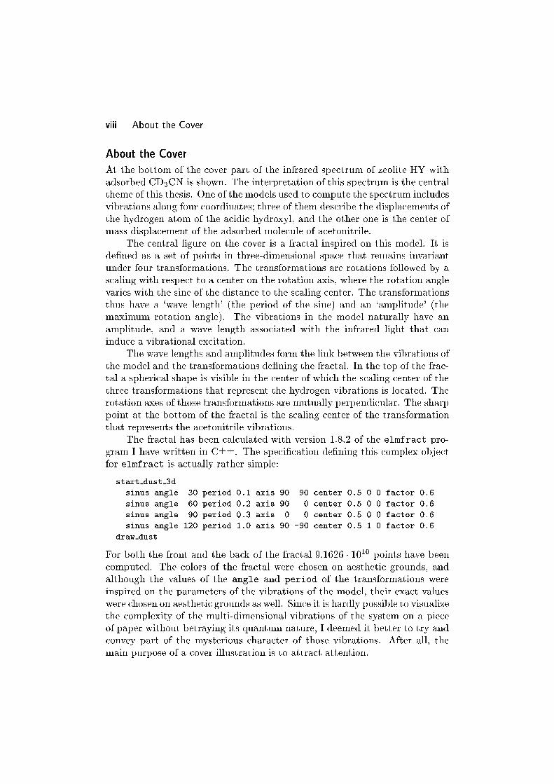
At the bottom of the cover part of the infrared spectrum of zeolite HY with
adsorbed CD3CN is shown. The interpretation of this spectrum is the central
theme of this thesis. One of the models used to compute the spectrum includes
vibrations along four coordinates; three of them describe the displacements of
the hydrogen atom of the acidic hydroxyl, and the other one is the center of
mass displacement of the adsorbed molecule of acetonitrile.
The central �gure on the cover is a fractal inspired on this model. It is
de�ned as a set of points in three-dimensional space that remains invariant
under four transformations. The transformations are rotations followed by a
scaling with respect to a center on the rotation axis, where the rotation angle
varies with the sine of the distance to the scaling center. The transformations
thus have a `wave length' (the period of the sine) and an `amplitude' (the
maximum rotation angle). The vibrations in the model naturally have an
amplitude, and a wave length associated with the infrared light that can
induce a vibrational excitation.
The wave lengths and amplitudes form the link between the vibrations of
the model and the transformations de�ning the fractal. In the top of the frac-
tal a spherical shape is visible in the center of which the scaling center of the
three transformations that represent the hydrogen vibrations is located. The
rotation axes of those transformations are mutually perpendicular. The sharp
point at the bottom of the fractal is the scaling center of the transformation
that represents the acetonitrile vibrations.
The fractal has been calculated with version 1.8.2 of the elmfract pro-
gram I have written in C++. The speci�cation de�ning this complex object
for elmfract is actually rather simple:
start dust 3d
sinus angle 30 period 0.1 axis 90 90 center 0.5 0 0 factor 0.6
sinus angle 60 period 0.2 axis 90 0 center 0.5 0 0 factor 0.6
sinus angle 90 period 0.3 axis 0 0 center 0.5 0 0 factor 0.6
sinus angle 120 period 1.0 axis 90 -90 center 0.5 1 0 factor 0.6
draw dust
For both the front and the back of the fractal 9:1626 � 1010 points have beencomputed. The colors of the fractal were chosen on aesthetic grounds, and
although the values of the angle and period of the transformations were
inspired on the parameters of the vibrations of the model, their exact values
were chosen on aesthetic grounds as well. Since it is hardly possible to visualize
the complexity of the multi-dimensional vibrations of the system on a piece
of paper without betraying its quantum nature, I deemed it better to try and
convey part of the mysterious character of those vibrations. After all, the
main purpose of a cover illustration is to attract attention.

1Introduction
This thesis is about quantum chemical calculations of infrared spectra of an
acidic hydroxyl group in a zeolite, with adsorbed acetonitrile. In this intro-
duction I will explain the concepts printed in slanted type in the previous
sentence. After that, a brief discussion of infrared spectra that have been
measured of acidic zeolites with adsorbed acetonitrile follows. Finally there
is an overview of the rest of the thesis.

2 Chapter 1: Introduction
1.1 Quantum Chemistry
Chemistry studies the structure of substances, and the chemical reactions
that convert substances into other substances. This is done on the one hand
by conducting experiments, and on the other hand by developing theoretical
models that explain them. Neither activity is useful without the other. It is
essential to have experimental data to check the validity of theoretical models,
and at the same time theoretical models are necessary to think about the
results of experiments, and to draw conclusions of more general importance. A
good theory is a very compact way to describe a large number of experiments,
with good accuracy. It should also be able to predict the outcome of newly
designed experiments.
The generally accepted theoretical model of chemical substances is the
atomic view of matter. In this model all matter consists of atoms. These atoms
consist of atomic nuclei and electrons, and they can combine into molecules
by forming chemical bonds. How chemical bonds are formed is described
by a theory called quantum mechanics. The central equation in quantum me-
chanics is the Schr�odinger equation, which, combined with the Pauli principle,
gives a complete description of how atomic nuclei and electrons behave. There
are only two problems with it.
The �rst problem with the Schr�odinger equation is that it is too hard.
In general it can only be solved exactly for systems with a small number
of particles (one or two). Application of quantum mechanics on chemically
interesting systems is possible only using approximations of the solution to
the Schr�odinger equation. This activity has become a branch of science in its
own right, quantum chemistry.
The second problem with the Schr�odinger equation is that it is known
to be wrong. It is regular practice in chemistry and physics to use a the-
ory that is wrong, and not particularly worrying as long as you are aware
on what type of problems the theory can be applied, and when it starts to
produce less accurate or even completely false results. The main problem
is that according to the Schr�odinger equation particles can reach velocities
larger than the speed of light, but according to experiments, they cannot.
For a quantum chemist, this becomes a problem in the calculation of the be-
haviour of electrons in heavier atoms. There are two remedies. Instead of
the Schr�odinger equation, one can use the Dirac equation, which doesn't have
this problem. The Dirac equation is even harder to solve than the Schr�odinger
equation. Alternatively, ad hoc, `relativistic corrections' can be made when
solving the Schr�odinger equation. The quantum chemical calculations in this
thesis employ the Schr�odinger equation without relativistic corrections, which
is excusable because the atoms described are light, and the velocities of the
particles involved do not approach the speed of light.

Quantum Chemistry 3
The Schr�odinger equation can be formulated in di�erent coordinate sys-
tems, or representations. The representation used most in this thesis is the
spatial coordinate representation, which is suitable for bound systems. An
example of a bound system is a hydrogen atom, where the electron has an
energy below the ionisation potential. If the energy of the electron becomes
higher than the ionisation potential, the electron can move arbitrarily far away
from the nucleus, and they form no longer a bound system.
The solutions to the Schr�odinger equation are wave functions. These
wave functions are the eigenfunctions of the Hamiltonian, a mathematical
operator that represents the energy of the system. Integration of the square
of the wave function over a certain area of the coordinate space, yields the
chance that the coordinates of the system correspond to that area if they
were measured. With the wave functions expectation values for the di�erent
coordinates can be computed. In this respect there is a fundamental di�erence
with classical mechanics, where, in principle, exact values of the coordinates
can be computed.
If there are no time-dependent external forces on a system, the Hamil-
tonian is not a function of time, and neither are the expectation values of
the coordinates. The Schr�odinger equation can then be split into a time-
independent and a time-dependent part. The time-dependent part is trivial
to solve for time-independent Hamiltonians, and often quantum chemists only
deal with the time-independent Schr�odinger equation.
For a bound system with a time-independent Hamiltonian, the total en-
ergy can only have a limited number of discrete values, and not any in between.
We then say that the energy is quantized. This means there is only a lim-
ited number of states for bound systems, with corresponding wave functions.
Quantum chemists often are only interested in the bound state with lowest en-
ergy, the ground state. The states with higher energy are called excited states.
In this thesis only ground states for the electronic structure were computed,
but many excited states for the nuclear vibrations.

4 Chapter 1: Introduction
1.2 Infrared Spectra
1.2.1 Quantum Chemical Calculation of Infrared Spectra
The theory of Maxwell describes electromagnetic radiation as mutually per-
pendicular electric and magnetic �elds, oscillating with the same frequency.
In a vacuum these oscillating �elds travel with the speed of light in a direction
perpendicular to their oscillation directions. Electromagnetic radiation carries
energy. Molecules can absorb this energy in packets, photons, that carry an en-
ergy equal to the frequency � of the radiation times Planck's constant h. This
means that under certain conditions a molecule in a state with energy E0 can
absorb a photon, and then reach a state with energy E1, if h� = E1�E0. This
condition, known as Bohr's frequency rule, shows that only radiation of very
speci�c frequencies can be absorbed by molecules. Whether the molecule can
actually absorb the radiation also depends on the interaction of the molecule
in the di�erent states with the electromagnetic �eld.
Atoms in molecules do not sit still; they vibrate with respect to each
other. Because atoms in molecules form a bound system, the vibrational en-
ergy of the molecule is quantized. The di�erences between vibrational energy
levels are in the range of the energy of photons of infrared light, which is elec-
tromagnetic radiation with frequencies just below the range of visible light.
If infrared light of a certain frequency is absorbed by a molecule, this shows
that there are vibrations (or rotations) with corresponding energies in the
molecule. An infrared spectrum of a substance is obtained measuring the ab-
sorption of infrared light as a function of its frequency. Each absorption peak
corresponds with a particular vibration (or rotation) of the molecule, and the
complete spectrum provides a means of identi�cation of this molecule.
In the calculations of infrared spectra in this thesis, a number of ap-
proximations is made. The motion of electrons is treated separately from the
motion of the nuclei. Because the nuclei are three to four orders of magnitude
heavier than the electrons, they can be assumed to stand still in the calcula-
tion of the electronic wave function. This is known as the Born-Oppenheimer
approximation. For a certain set of nuclear positions the wave function of
the electronic ground state is computed, yielding the energy and dipole for
this geometry. Excited states of the electronic wave function are usually not
necessary for the calculation of infrared spectra, because they are separated
much further in energy than the vibrational states. In the calculation of the
electronic wave functions there are more approximations. The wave function
is expanded in a so-called basis set. This means that it is written as a linear
combination of a limited number of basis functions, that have the shape of
wave functions themselves. Then approximative methods are used to �nd the
best solution that can be described within the basis set, notably the Hartree-
Fock method and Density Functional Theory.

Infrared Spectra 5
For the solution of the vibrational Schr�odinger equation the energy of the
molecule as a function of the nuclear coordinates is needed. This is obtained by
calculation of the electronic energy for a number of geometries. In this thesis
the potential energy is �tted with a polynomial (yet another approximation).
Like the electronic Schr�odinger equation, the vibrational Schr�odinger equation
has been solved with a basis set, but no further approximations were made to
obtain the best solution in the basis set.
One other quantity besides the separation between the vibrational levels
is needed to be able to calculate an infrared spectrum: the absorption inten-
sity. If a photon of the right frequency interacts with a molecule, its electric
�eld needs to exert a force that `pushes' the molecule from the initial state
to the �nal state. If it does not do that, no transition will take place. How a
molecule interacts with an electric �eld is primarily determined by its dipole.
The dipole as a function of the nuclear coordinates is calculated together with
the energy in the electronic structure calculations, and, in this thesis, �tted
with a polynomial. Whereas for the calculation of electronic and vibrational
wave functions the time-independent Schr�odinger equation suÆced, for the
calculation of absorption intensities the time-dependency of the Schr�odinger
equation needs to be considered explicitly, because the oscillating electric �eld
of the radiation enters the Hamiltonian. This is done with perturbation the-
ory, a �nal approximation which gives us an expression to compute absorption
intensities from the dipole surface and the vibrational wave functions of the
involved states.
1.2.2 The Harmonic Approximation
The quantum chemical calculation of infrared spectra is often done in the har-
monic approximation. This approximation is present as an option in gener-
ally available quantum chemical computer programs like GAMESS and Gaus-
sian98. Most of the spectra in this thesis have not been computed with this
approximation, but it serves well as a reference point to describe vibrational
spectra.
In the harmonic approximation it is assumed that the potential energy
surface can be written as a second order polynomial in the displacements
of the atoms in the molecule, and the dipole surface as a linear function of
the atomic displacements in the molecule. Because of this double condition,
it is sometimes called the double harmonic approach. If in the calculation of
infrared spectra higher than quadratic terms in the potential energy are taken
into account, these are called mechanical anharmonicities, and if higher than
�rst order terms are used for the dipole surface, they are sometimes referred
to as electronic anharmonicities.
A very nice property of the harmonic approximation is that it yields a
vibrational Schr�odinger equation that can be solved exactly. To do this, the

6 Chapter 1: Introduction
Hamiltonian is written in terms of normal coordinates. These coordinates are
linear combinations of atomic displacement coordinates. They are determined
in such a way that the Hamiltonian can be written as a sum of smaller Hamil-
tonians, each of which only contains a potential energy term and a kinetic
energy term in only one of the normal coordinates. As a consequence, the
vibrational Schr�odinger equation can be split into a set of one-dimensional
vibrational Schr�odinger equations that can be solved separately. The normal
coordinates de�ne the movements of the atoms that belong to eigenmodes of
the molecule in the harmonic approximation, which are often referred to as
normal modes. The one-coordinate Schr�odinger equations each yield a set of
one-dimensional wave functions, also known as Hermite functions. The solu-
tions of the full harmonic vibrational Schr�odinger equations can be written as
products of Hermite functions of all the normal coordinates.
Normal modes have an in�nite number of one-dimensional vibrational
wave functions associated with them. The energy of a one-dimensional har-
monic vibrational wave functions is equal to (n+ 12)h�, where n is the quan-
tum number, � the frequency of the mode, and h is Planck's constant. These
quantum numbers are integral numbers ranging from 0 to 1, so even in the
ground state (n = 0) there is always a �nite amount of vibrational energy
present ( 12h�), called the zero-point energy. From the expression for the en-
ergy, it is also clear that the di�erence in energy between any two adjacent
levels is h�.
n = 0
n = 1
n = 2
n = 3
Hermite Functions
n = 0
n = 1
n = 2
n = 3
Squared Hermite Functions
Figure 1. The thick lines depict the �rst four Hermite functions, and the same
functions squared. The thin lines depict the harmonic potential and the lowest four
energy levels. Further description in the text.
In Fig. 1 the �rst four Hermite functions and their squares are drawn
into a graph of the harmonic potential with the four lowest energy levels. On
the horizontal axis the coordinate is plotted (e.g., the distance between two
atoms). The minimum of the potential corresponds to the equilibrium value of
the coordinate. The distance between the minimum of the potential and the
�rst horizontal line depicting the lowest energy level represents the zero-point

Infrared Spectra 7
energy. The Hermite functions and their squares have been drawn such that
their origin lies on the line representing their energy. The squared Hermite
functions correspond to the chance density of �nding a particular value of the
coordinate when a measurement is done. For the lowest level (n = 0) it is
most likely to measure the equilibrium value of the coordinate, whereas for
the other levels a di�erent value is more likely. For the levels with n = 1 and
n = 3 the chance to measure the equilibrium value for the coordinate is even
zero.
In the double harmonic approach, only those transitions where the quan-
tum number of exactly one normal mode increases by one have non-zero ab-
sorption intensity. Other transitions are called `forbidden'. In practice this
means that in this approximation only the transitions from the ground state to
the �rst excited state in one of the normal modes are present in a computed
infrared spectrum. In a more general context transitions from the ground
state to the �rst excited state in one mode are called fundamentals. In real
infrared spectra it is sometimes also possible to observe transitions from the
ground state to the second (or higher) excited state of a mode, which is called
an overtone, or from the ground state to a state where two (or more) modes
are excited, which is called a combination band. In real infrared spectra it
is often also possible to see hot bands, which are transitions from an already
excited state to an even more excited state. Hot bands that involve a tran-
sition from a state excited in one mode to a state excited in another mode
have a frequency that is the di�erence from transitions to these states from
the ground state, and are hence called di�erence bands. In the harmonic ap-
proach the hot bands that have non-zero absorption intensity always have a
frequency that is exactly equal to a fundamental, which is generally not the
case in real infrared spectra.
The harmonic approximation is quite useful for molecules in which the
chemical bonds between the atoms are relatively strong, to describe the fun-
damentals of the infrared spectrum. The reason it works well in this case, is
that the average displacement of the atoms from their equilibrium position is
small, and the part of the potential energy they are subject to can be modelled
well with a quadratic curve. In general stretch mode transitions computed in
the harmonic approach are somewhat too high in frequency, whereas bending
modes can be either too high or to low.

8 Chapter 1: Introduction
Figure 2 gives an impression how one-dimensional harmonic wave func-
tions relate to their anharmonic counterparts for a given potential. Let us
assume it is the potential for a diatomic molecule as a function of the distance
between the atoms.
Harmonic Anharmonic
Figure 2. The square of the �rst four vibrational wave functions for a one-dimension-
al potential. The left �gure shows the harmonic approximation to the anharmonic
potential and wave functions in the right �gure.
The anharmonic potential in this �gure is steeper than the harmonic one for
small values of the coordinate, because if two atoms are nearing each other
closely, the energy will approach in�nity (neglecting nuclear reactions). For
larger values of the stretch coordinate the potential levels o� to a constant
value, which corresponds to the situation where the bond is broken. From
Fig. 2 it can be seen that higher excited states are increasingly worse described
by the harmonic approximation. Also the wave functions are no longer sym-
metric with respect to the equilibrium distance, and the expectation value of
the distance becomes longer in higher excited states.
Hydrogen bonded molecules provide a typical example of systems where
the harmonic approximation to calculate infrared spectra breaks down. The
reason is that the potential to which the hydrogen atom is subject becomes
very shallow and anharmonic around the minimum, and the hydrogen atom
itself is very light. As a result the hydrogen atom has a relatively large
displacement, in con ict with the basic underlying assumption of the harmonic
approximation.

Infrared Spectra 9
1.2.3 Fermi Resonance
Both Raman spectroscopy and infrared spectroscopy provide information on
vibrational and rotational energy levels. Raman spectra are obtained illumi-
nating a sample with visible or ultraviolet light of a certain frequency, and
measuring the intensity of the scattered light. Part of the scattered photons
lose energy because molecules are vibrationally (or rotationally) excited dur-
ing the scattering, yielding the so-called Stokes lines. At higher frequencies
than the incident light, the anti-Stokes lines are found, which are produced
by photons that gain energy because they are scattered by a molecule that
changes from a higher vibrational or rotational energy state into a lower one.
Raman and infrared spectroscopy can be complementary to each other,
because the selection rules that determine if a certain transition occurs in
the spectrum are di�erent. Vibrational transitions are present in infrared
spectroscopy if they are accompanied by a change in the dipole moment, and in
Raman spectroscopy if they are accompanied by a change in the polarizability
of the molecule.
Fermi �rst described a phenomenon in the Raman spectrum of CO2[1]
that now bears his name. CO2 has three fundamental frequencies; one at
667.5 cm�1 due to two perpendicular bends, one at 2350 cm�1 due to an
asymmetric stretch, and one about 1300 cm�1 due to a symmetric stretching
mode. In the infrared spectrum the symmetric stretch is inactive, but in the
Raman spectrum there are two approximately equally intense lines around
1300 cm�1. This phenomenon occurs because there is a resonance between
the �rst excited state of the symmetric stretch and the second excited state
of the bending modes, which under normal circumstances would be expected
to yield a weak absorption around 2 � 667:5 cm�1 = 1335 cm�1. Because the
two levels would accidentally have almost the same energy, and they share a
compatible symmetry, they combine into two new states. Both states are a
combination of the �rst excited state of the symmetric stretch and the second
excited state of the bend. One of the states is somewhat lower in energy than
the `unperturbed' states, and the other is somewhat higher in energy. This
explains why there are two absorption lines of approximately equal strength,
due to transitions from the ground state to the two resonating states.
Fermi resonance cannot be described well in the harmonic approximation
to the calculation of infrared spectra. In the quantum mechanical description
of the phenomenon[2] it can be shown that Fermi resonance is due to anhar-
monic terms in the potential energy. The di�erences between the harmonic
wave functions and the solutions of the full anharmonic Hamiltonian become
very large if the energies of two (or more) harmonic wave functions happen to
be near each other, and the harmonic wave functions are no longer a useful
approximation.
10 Chapter 1: Introduction
1.3 Zeolites with Adsorbed Acetonitrile
The main dish of this thesis consists of quantum chemical calculations of the
infrared spectrum of an acidic hydroxyl of a zeolite with adsorbed acetonitrile.
This section is devoted to a description of what zeolites are, why one would
want to adsorb acetonitrile in them, and what the experimentally measured
infrared spectra look like.
1.3.1 Zeolites
Imagine a crystalline material with an overall chemical composition very sim-
ilar to sand (SiO2), with cavities and channels in it, and replace some of the
silicon with aluminium and a cation. There you have your typical zeolite. The
silicon and aluminium atoms are tetrahedrically surrounded by oxygen atoms,
and therefore often named `T-atoms'. The oxygen atoms take bridging posi-
tions between two silicon atoms, or between a silicon atom and an aluminium
atom. The fact that aluminium atoms with only one bridging oxygen do not
occur is known as L�owenstein's rule. If the additional cation that comes with
each aluminium atom introduced in the zeolite is a proton, these protons sit
on bridging oxygen atoms between a silicon and an aluminium atom. The
bridging hydroxyl is a Br�nsted acid, and the Al(OH)Si group is often re-
ferred to as the Br�nsted acid site of a zeolite. Br�nsted acid sites in zeolites
contain oxygen atoms with three bonds. Since this is a rather `untraditional'
situation, some people prefer to describe it as an SiOH group where the hy-
droxyl has a dipolar interaction with the nearby aluminium atom, which then
has three bonds with bridging oxygen atoms.
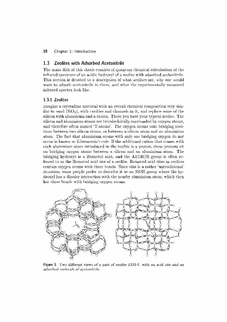
Figure 3. Two di�erent views of a part of zeolite ZSM-5, with an acid site and an
adsorbed molecule of acetonitrile.

Zeolites with Adsorbed Acetonitrile 11
Zeolites have fascinating crystal structures. The `zeolite atlas' [3] of 1992
lists 67 di�erent crystal structures known for zeolites. Besides for looks, ze-
olites are also popular in a wide range of applications. In washing powders
zeolites are used as ion exchangers, to remove calcium from the water. In the
petrochemical industry zeolites are used as catalysts, and as catalyst carriers.
They are very interesting for catalysis for several reasons. Due to their pore
structure zeolites have a high internal surface area. The pores in zeolites have
very speci�c sizes of molecular dimensions, which enables selectivity based on
the size and shape of reactants. Finally zeolites are very interesting because
they can be solid acids, which means that you can carry out an acid-catalysed
reaction where the acid can easily be separated from the liquid or gaseous
product.
1.3.2 Acetonitrile as a Probe Molecule
The acidity of zeolites inspired the research presented in this thesis. Di�erent
types of acidic zeolites have di�erent reactivity with respect to acid-catalysed
reactions. To �nd an explanation for these di�erences, one of the aspects that
needs to be investigated is the acidity of the Br�nsted acid sites in the zeolites.
It cannot be done with the methods traditionally used for acids in liquid form,
like measuring the pH in solution. A way to investigate the acidity is to adsorb
weakly basic molecules on the acid sites in the zeolites, and then study the
infrared spectrum of the acidic OH group. Upon absorption of a molecule
the OH stretch frequency goes down, and the size of the downward shift is a
measure of the acidity of the OH group.
Acetonitrile is an interesting basic probe molecule for these experiments.
On the one hand it is only just not strong enough a base to abstract a proton
from the acid site. On the other hand acetonitrile is so strong a base that it
changes the infrared spectrum of the acidic OH group dramatically. The single
OH stretch peak normally found in an infrared spectrum of an acidic zeolite
at 3610 cm�1 is replaced with two very broad bands around 2400 cm�1 and
2800 cm�1. The main subject of this thesis is to reproduce this spectrum with
quantum chemical methods, and to explain why it has its particular shape.
The changes in the infrared spectrum of an acidic zeolite caused by ace-
tonitrile adsorption are not unique for acetonitrile. Other molecules of com-
parable basicity yield similar spectra. The reason acetonitrile was chosen for
the calculations in this thesis, is that it is the smallest molecule that shows
this behaviour and has no further complications. Small molecules are good
for quantum chemists, because they allow us to use more accurate methods
that require relatively long computation time. In this case small molecules
are also good as probe molecules for experimentalists: larger molecules may
not be able to reach every acid site inside a zeolite.

12 Chapter 1: Introduction
1.3.3 Infrared Spectra of HY and ZSM-5 with Acetonitrile
Infrared di�erence spectra for the adsorption of acetonitrile in zeolite HY
at three di�erent loadings are shown in Fig. 4.[4] The upper spectrum has
the highest loading of acetonitrile, the middle one has a lower loading, and
the bottom spectrum has the smallest loading. Peaks that disappear upon
adsorption are plotted downwards, and peaks that appear are plotted upwards.
1500 2000 2500 3000 3500 4000wave number
a
b
c
3550
3630
Figure 4. Infrared di�erence spectra of the adsorption of CD3CN on zeolite HY. The
wave numbers are in cm�1 . The spectra were measured at room temperature, with
0.8 mbar CD3CN pressure (a), with 0.05 mbar CD3CN (b), and after 30 minutes of
evacuation (c).
The sharp peaks around 2300 cm�1 are due to the CN stretch interacting
with di�erent sites in the zeolite, and the peak at 2114 cm�1 is due to the
CD3 symmetric stretch. These modes are discussed in detail in Ref. 4.
Two peaks at 3550 cm�1 and 3630 cm�1 disappear upon adsorption. They
are due to the OH stretch mode of two di�erent types of acid sites in zeolite
HY. The 3630 cm�1 stretch mode is typical for a bridging hydroxyl in zeo-
lites. Relatively small variations exist, e.g., in ZSM-5 the mode is found at
3610 cm�1. The 3550 cm�1 mode is speci�c for HY. It too stems from a bridg-
ing hydroxyl, but from one situated in a position where it has a hydrogen bond
type of interaction with another bridging oxygen atom from the zeolite lattice.
As discussed before, such an interaction lowers the OH stretch frequency.
The main feature in these infrared spectra is formed by the two broad
bands that have their maxima at 2400 cm�1 and 2750{2900 cm�1. There are
di�erent arguments to assume that they both stem from one complex of an
acidic hydroxyl with acetonitrile, instead of each from a di�erent complex.
Firstly the bands appear and grow simultaneously with the disappearance of
the unperturbed OH stretch bands at 3550 cm�1 and 3630 cm�1, and it is
not possible to desorb acetonitrile in such a way that only one of the two
bands remains. Secondly very similar bands are found for a range of di�erent

Zeolites with Adsorbed Acetonitrile 13
zeolites, which rules out the possibility that acid sites in speci�c positions are
responsible for the two di�erent broad bands. Thirdly very similar spectra
are found for di�erent adsorbing molecules of comparable basicity, which rules
out two speci�c di�erent adsorption modes of acetonitrile to be responsible
for the two broad bands.[5]
In Fig. 4 the di�erence in acidity between the two types of hydroxyls
(3550 cm�1 vs. 3630 cm�1) can be deduced from a comparison of the spectra
at di�erent loadings. At low acetonitrile loading (spectrum (c)) mostly hy-
droxyls with an unperturbed stretch frequency of 3630 cm�1 are occupied. At
higher acetonitrile loading the hydroxyls with unperturbed stretch frequency
at 3550 cm�1 are occupied too. Their stretch frequency shifts considerably
less upon adsorption of acetonitrile, and as a result the maxima of the two
broad bands shift to higher wave numbers at higher acetonitrile loadings. Both
the fact that the hydroxyls with unperturbed stretch frequency of 3630 cm�1
form complexes with acetonitrile more readily, and the fact that they exhibit
a larger shift of the stretch frequency upon adsorption of acetonitrile, indi-
cate that they are more acidic than the hydroxyls that have an unperturbed
stretch frequency of 3550 cm�1.
Figure 5 shows infrared di�erence spectra for the adsorption of deuterated
acetonitrile in zeolite ZSM-5, at three di�erent loadings, similar to Fig. 4.
Again at 2114 cm�1 the CD3 symmetric stretch of acetonitrile appears, and
around 2300 cm�1 there are CN vibrations visible from acetonitrile adsorbed
on di�erent sites.[4]
1500 2000 2500 3000 3500 4000wave number
a
b
c
3610
3745
Figure 5. Infrared di�erence spectra of the adsorption of CD3CN on zeolite ZSM-5.
The wave numbers are in cm�1 . The spectra were measured at room temperature,
with 1.1 mbar CD3CN pressure (a), with 0.05 mbar CD3CN (b), and after 30 minutes
of evacuation (c).
The disappearing peaks at 3610 cm�1 and 3745 cm�1 are due to the bridg-
ing hydroxyl and silanol (Si{OH) OH stretch modes, respectively. The bridg-
ing hydroxyl groups are more acidic, and are occupied signi�cantly at lower
14 Chapter 1: Introduction
acetonitrile loadings than the silanol groups. The shift of the OH stretch of the
silanol groups is much smaller than that of the bridging hydroxyl groups, and
is visible as one broad band with its maximum at approximately 3400 cm�1.
This band shows up only as a shoulder in the spectrum of HY. The reason
that the silanol groups are more prominently visible in the spectrum of ZSM-
5, is that the concentration of Br�nsted acidic sites is much smaller: in the
HY sample used the Si/Al ratio was 5.1, whereas in the ZSM-5 sample it was
52.[4]
The Br�nsted acid hydroxyls in ZSM-5 give rise to two broad bands
around 2400 cm�1 and 2800 cm�1, similar to the most acidic bridging hydrox-
yls from zeolite HY. In addition, and at the same time, a third band appears
around 1700 cm�1.
The bands around 2800, 2400, and 1700 cm�1, are often referred to as
A, B, and C-bands. Pelmenschikov et al.[4] proposed an explanation where
the entire A,B,C-system is in fact one broad band due a shifted OH stretch
mode, forming combination and di�erence bands with stretch modes of the
acetonitrile molecule with respect to the OH-group, including overtones of
this mode. In this view, there are so-called Evans windows around 1900
and 2600 cm�1. These Evans windows are due to a Fermi resonance of the
broadened OH stretch band with the �rst overtones of the OH in-plane and
out-of-plane bending, respectively (the `plane' referred to is the plane de�ned
by Si{O{Al of the acidic site). The resonance causes the absorption inten-
sity due to the OH stretch band to be shifted to lower and higher frequency
than the frequency of the `unperturbed' bending mode overtone with which
it resonates. Evans �rst described the occurrence of a similar `window' in the
infrared spectra of m-toluidine.[6]
Since in the A,B and A,B,C-spectra the absorption intensity is mainly
due to the OH stretching mode, the center of gravity of the two or three bands
is considered a measure for the imaginary unperturbed position of the shifted
OH stretch band. The shift is considered to be an indication of the acidity of
the OH group. Hence the proportion of the absorption intensity of the A band
versus the B and C bands gives information on the acidity of the involved OH
groups. If this is applied to the spectra of Fig. 4 of HY and Fig. 5 of ZSM-5
with acetonitrile, we can conclude that ZSM-5 contains more OH groups that
are more acidic than HY.

References 15
1.4 Contents of this Thesis
The previous section concludes the introductory material. The rest of the
thesis consists of the following. First there is chapter 2 which contains the
theoretical background of the calculations of infrared spectra presented in the
thesis. It is aimed at people with a basic understanding of quantum chemistry,
and should, in principle, provide them enough information to perform similar
calculations themselves.
Subsequently there are three chapters which are more or less copies of
articles written for a scienti�c journal. In chapter 3 the �rst calculations of
the infrared spectrum of a zeolite's Br�nsted OH with adsorbed acetonitrile
are presented. The models used in this chapter involve the dynamics of the
acidic hydrogen atom, and an intermolecular stretch mode of acetonitrile. The
zeolite is modelled with a cluster molecule, which is a relatively small molecule
that represents the acidic site in a zeolite. In chapter 4 the same molecular
model is used, but the dynamics of the oxygen atom of the acidic OH group
are now accounted for as well. Chapter 5 returns to the simpler dynamics
model of chapter 3, but the cluster molecule representing the zeolite is now
embedded in a molecular mechanics model of a substantial part of the zeolite.
Chapter 6 contains a general overview of the preceding three chapters, and
gives an overview of the conclusions.
There are two appendices describing the AnharmND program in the back
of the thesis. The �rst one is a manual, and the second one is a short guide for
someone who wants to use AnharmND to compute an infrared spectrum. If
you want to use the program, it is probably best to read the second appendix
�rst, and then the manual in the �rst appendix. The theoretical background
is in chapter 2.
The thesis ends with a summary in English and in Dutch, my Curriculum
Vitae, and an acknowledgement in Dutch.
References
[1] E. Fermi; Z. Physik, \�Uber den Ramane�ekt des Kohlendioxyds", 71,
250{259 (1931).
[2] G. Herzberg; Molecular Spectra and Molecular Structure II. Infrared and
Raman Spectra of Polyatomic Molecules; chap. II-5, van Nostrand, New
York, 1960.
[3] W. M. Meier, and D. H. Olson; Atlas of Zeolite Structure Types, Third
Revised Edition; Butterworth-Heineman, London, 1992.
[4] A. G. Pelmenschikov, R. A. van Santen, J. J�anchen, and E. L. Meijer;
J. Phys. Chem., \CD3CN as a Probe of Lewis and Br�nsted Acidity of
Zeolites", 97, 11071{11074 (1993). The infrared spectra shown in this

16 Chapter 1: Introduction
chapter were taken from this paper. All spectra have been measured by
Jos van Wolput, who also kindly provided the data for the �gures 4 and
5 in this chapter.
[5] C. Paz�e, S. Bordiga, C. Lamberti, M. Salvalaggio, A. Zecchina, and
G. Bellussi; J. Phys. Chem. B, \Acididc Properties of H-� Zeolite As
Probed by Bases with Proton AÆnity in the 118{204 kcal mol�1 Range:
A FTIR Investigation", 101, 4740{4751 (1997).
[6] J. C. Evans, and N. Wright; Spectrochim. Act., \A Peculiar E�ect in the
Infrared Spectra of Certain Molecules", 16, 352{257 (1960).
2Theory of the Computation of Infrared Spectra
Introduction
I have written a computer program `AnharmND' to compute infrared spec-
tra taking into account anharmonicities. This chapter provides some of the
theoretical background on which the computations of the program are based.
In AnharmND solutions for the time-independent Schr�odinger equation
for a limited set of coordinates are approximated. The coordinates are linear
combinations of cartesian atomic coordinates, the kinetic energy is expressed
in terms of products of the conjugated momenta of the coordinates, and the
potential energy is represented by a polynomial in the coordinates. The dipole
surface that is needed for the computation of infrared absorption intensities is
represented by polynomials for each component. The Schr�odinger equation is
solved with a variational approach where the wave functions are expanded in
a basis set of products of Hermite functions. The next section of this chapter
discusses how matrix elements of the Hamiltonian are computed. Then there
is a section about the computation of the potential energy and dipole surfaces
on a grid, and how they are �tted with polynomials in AnharmND. The
eigenvalue equation is solved with a Lanczos scheme or a modi�ed Lanczos
scheme, which is described in the fourth section of this chapter. Finally in
the last section the expressions to compute integrated infrared absorption
intensities are derived from time dependent perturbation theory.

18 Chapter 2: Theory of the Computation of Infrared Spectra
2.1 The Hamiltonian and its Matrix Elements
2.1.1 The Vibrational Hamiltonian in Internal Linear Coordinates
Consider a system of N atoms with cartesian coordinates x1; : : : ; x3N , masses
m1; : : : ;mN , and M linear internal coordinates q1; : : : ; qM . In this paragraph
we will express the vibrational Hamiltonian in the coordinates fqig and their
conjugate momenta.
De�ne the matrix A such that
Aq = x: (1)
Note that because the coordinates fqig are linear, the elements of A are con-
stant. The Lagrangian L can be expressed in terms of the internal coordinates
fqig. First an expression for the kinetic energy T is derived:
T = 12
3NXi=1
mdi=3e _x2i
= 12
3NXi=1
mdi=3e
n MXj=1
Aij _qj
o2
= 12
MXj=1
MXk=1
n 3NXi=1
AijAikmdi=3e
o_qj _qk
= 12
MXj=1
MXk=1
Gjk _qj _qk;
(2)
where the matrix G is de�ned by
Gjk �3NXi=1
mdi=3eAijAik: (3)
The Lagrangian is de�ned as the di�erence between the kinetic energy T and
the potential energy V :
L = T � V = 12
MXj=1
MXk=1
Gjk _qj _qk � V (fqig): (4)

The Hamiltonian and its Matrix Elements 19
The momenta fpig conjugated to the coordinates fqig are found by di�eren-
tiation of the Lagrangian. Taking into account that G is symmetrical this
yields
pl =@L
@ _ql=
MXj=1
Gjl _qj ; (5)
so that we have
_qi =
MXj=1
(G�1)ijpj ; (6)
where (G�1)ij denotes an element of the inverse of G. Now the kinetic energy
can be written as a function of momenta:
T = 12
MXi=1
MXj=1
(G�1)ijpipj ; (7)
and the classical Hamiltonian becomes
H = T + V = 12
MXi=1
MXj=1
(G�1)ijpipj + V (fqig): (8)
Because the coordinates we are using are linear the matrices A and G are
constant, and we can convert the classical Hamiltonian Eq. 8 into a quan-
tum mechanical one by substitution of the momenta pj with the operators
(�h=i)=(d=dqj). If the coordinates used are not linear, the matrices A and G
become functions of fqjg, and the conversion of Eq. 8 into a quantum me-
chanical Hamiltonian becomes more complicated because qj and (�h=i)(d=dqj)
do not commute. The construction of a quantum mechanical Hamiltonian in
general coordinates has been described by Podolsky.[1]

20 Chapter 2: Theory of the Computation of Infrared Spectra
2.1.2 The Second Quantization Formalism for a Harmonic Oscillator
To facilitate calculations with vibrational wave functions, it can be advan-
tageous to switch from coordinates and conjugated momenta to a represen-
tation in creation and annihilation operators,[2] also known as the second
quantization formalism. These operators are de�ned in the context of a one-
dimensional harmonic oscillator. Consider a harmonic oscillator along coor-
dinate q with a reduced mass �, force constant � and conjugated momentum
p. The Hamiltonian for this oscillator is given by
H =p2
2�+ 1
2�q
2: (9)
The annihilator operator a and the creator operator ay are each other's Her-
mitian adjoints, de�ned as follows:
a ��!q + ip
p2��h!
ay �
�!q � ipp2��h!
:
(10)
where ! is de�ned asp�=�, �h is Planck's constant h divided by 2�, and
i2 = �1. Note that these operators are dimensionless by this de�nition. The
spatial coordinates and conjugated momenta can be expressed in creator and
annihilator operators:
q =
s�h
2�!(ay + a)
p = i
r�!�h
2(ay � a):
(11)
The quantum mechanical operators q and p do not commute, because in the
spatial coordinate representation p is given by p = (�h=i)(d=dq). From this the
commutator of q and p can be computed:
[q; p] � qp� pq =�h
i
(qd
dq
�d
dq
q) =�h
i
(qd
dq
� (1 + q
d
dq
)) = ��h
i
= i�h (12)
From the commutation relationship between a coordinate and its conjugated
moment, we �nd the commutation relation for creation and annihilation op-
erators.
[q; p] = i�h , [a; ay] = 1 (13)

The Hamiltonian and its Matrix Elements 21
The Hamiltonian Eq. 9 can now be rewritten in terms of creation and anni-
hilation operators:
H = 12�h!(aya+ aa
y) = �h!(aya+ 12): (14)
In Dirac notation, an eigenfunction of a harmonic oscillator is written as jni,where n is the excitation level or number of phonons or quanta in the state.
The e�ect of a and ay on a state jni is to remove or add a quantum, hence
their names.ajni =
pnjn� 1i
ayjni =
pn+ 1jn+ 1i
(15)
Matrix elements of combinations of annihilation and creation operators
are easily computed if they are put in the normal product form. A normal
product is de�ned by
n[�; �] � (ay)�(a)�: (16)
For multiplication we have the following relations (using Eq. 13):
ayn[�; �] = n[�+ 1; �]
an[�; �] = n[�; � + 1] + � n[�� 1; �]:(17)
From Eq. 11 and Eq. 17 we then get for q and p:
q =
s�h
2�!(n[1; 0] + n[0; 1]) (18a)
q n[�; �] =
s�h
2�!(n[�+ 1; �] + n[�; � + 1] + � n[� � 1; �]) (18b)
p = i
r�!�h
2(n[1; 0]� n[0; 1]) (19a)
p2 = � 1
2�!�h(n[2; 0]� 2 n[1; 1]� n[0; 0] + n[0; 2]): (19b)
Eq. 18 can be used recursively to express powers of q into normal products
of annihilation and creation operators. For the kinetic energy only p and p2,
given by Eq. 19, are of practical importance.
A simple analytical expression for matrix elements of normal products
can be deduced from Eq. 15:
hnjn[�; �]jmi =�q
n!m!(n��)!(m��)!
if n� � = m� � � 0;
0 otherwise.(20)

22 Chapter 2: Theory of the Computation of Infrared Spectra
2.1.3 A Basis Set for Multidimensional Vibrational Wave Functions
We approximate eigenfunctions of the Hamiltonian Eq. 8 with a variational
approach, expanding them in a basis set of products of Hermite functions of
each coordinate qi. Hermite functions are the eigenfunctions of a harmonic
oscillator. We need to be able to compute matrix elements of them, which
means we need to choose the � and ! parameters from Eq. 18 and Eq. 19. To
do this we split up the Hamiltonian in two parts, a `sum of harmonics' part
Hh and a `anharmonic plus coupling' part Ha+c:
H = Hh +Ha+c =
MXj=1
�12(G�1)jjp
2j +
12�jq
2j
+Ha+c: (21)
Ha+c contains the kinetic energy terms 12(G�1)jkpjpk and the bilinear po-
tential energy terms �jkqjqk with j 6= k, and the anharmonic terms in the
potential energy. In general it is best to choose the coordinates in such a way
that the o�-diagonal terms of the kinetic energy and the o�-diagonal bilinear
terms of the potential energy are zero. This means that the normal coordinates
for the used set of internal coordinates are used. There are occasions that this
may not be the best choice, e.g., in the description of a double well potential.
This chapter describes the method that is implemented in AnharmND, and
the program does not compute the normal coordinates by itself. This should
be done by the user.
The eigenfunctions � of Hh are of the form
�(n1; : : : ; nM ) =
MYj=1
�
(nj)j (qj) = jn1; : : : ; nmi; (22)
where �(nj)j (qj) is the eigenfunction of a harmonic oscillator in coordinate qj ,
containing n quanta. From comparison of Eq. 9 with Eq. 21 we determine the
parameters of these functions as
�j^
=1
(G�1)jjand !j =
q�j=�j
^
=
q�j(G�1)jj : (23)
The eigenfunctions of the complete Hamiltonian Eq. 8 are approximated by
a linear combination of the basis functions �. These basis functions form a

Fitting the Potential Energy and Dipole Surfaces 23
good basis set if the potential V has a minimum for q = 0. Eq. 18 and Eq. 19
now become
qj =
r12�h
q(G�1)jj=�j
�nj[1; 0] + nj[0; 1]
�(24a)
qj nj[�; �] =
r12�h
q(G�1)jj=�j
�nj[�+ 1; �] + nj[�; � + 1] + � nj[� � 1; �]
�(24b)
pj = i
r12�h
q�j=(G�1)jj
�nj[1; 0]� nj[0; 1]
�(25a)
p2j = �
12�h
q�j=(G�1)jj
�nj[2; 0]� 2 nj[1; 1]� nj[0; 0] + nj[0; 2]
�: (25b)
2.2 Fitting the Potential Energy and Dipole Surfaces
2.2.1 Considerations on Grids and Polynomials
AnharmND �ts potential energy and dipole surfaces speci�ed on a grid to
polynomials. The grid should cover the area where the wave functions of in-
terest and the used basis functions have non-negligible amplitude. To be able
to construct the grid this way, it is necessary to know approximately what the
fundamental frequencies of the modes being studied are. This information can
be obtained from a normal mode analysis with a standard quantum chemical
program like Gaussian or ADF, or by a numerical calculation of the force con-
stants. The harmonic force constants are the parameters that determine the
basis functions in AnharmND, together with the reduced masses. From them,
the r.m.s. (root-mean-square) width of the basis functions can be computed:
2ph�ijq2j�ii = 2
s(i+ 1
2)�h
p��
= 2
s(i+ 1
2)�h
2���: (26)
In this expression j�ii is the ith order Hermite function of coordinate q, � is
the reduced mass, � the force constant, � the frequency, �h Dirac's constant,
and � the ratio of the circumference of a circle and its diameter. It appears
that the grid needs to cover about two to four times the r.m.s. width of the
highest order basis function. No hard rules can be given.
The advantage of a polynomial as a functional form to �t a potential or
dipole component, is that it has no bias to a particular shape. Most potential
wells are well suited for �tting with a polynomial. The biggest disadvantage
in AnharmND is the behaviour of polynomials outside the area of the grid
points: they go either to +1 or to �1. If the polynomial describing the
24 Chapter 2: Theory of the Computation of Infrared Spectra
potential goes to �1 for certain coordinate values this poses problems if
there are basis functions that have non-negligible amplitude there. Unphysical
wave functions with low energy will be calculated that can be recognized by
high order Hermite functions in the basis functions with large coeÆcients.
If it occurs, increasing the basis set will give a continuously lower ground
level involving the highest order Hermite functions from the basis set. To
prevent this situation, we start by only using polynomials of which the highest
order terms are of even order, and try to choose the grid in such a way that
the coeÆcients of those terms are positive. If this is not possible, the basis
functions must be chosen in such a way that they have no large amplitude in
the area where the �tted potential has unphysically low values.
The number of points in a grid is a compromise between accuracy and
computer time. To be able to include anharmonic e�ects, and to �t with an
even order polynomial, the smallest number of points that can be used is �ve
along each mode, with a fourth order polynomial. Though this seems a small
number, it is in fact quite large once multiple dimensions come into play. If
�ve points along each mode are used in four dimensions and a regular grid
is constructed, the grid contains 54 = 625 points. The next logical grid size
would be 74 = 2401, which explains why in this thesis �ve points along each
mode has been deemed plenty. It should be noted that the number of grid
points can be lowered leaving out the points of the grid where more than
one coordinate has an extreme value, since these points tend to have such
high energy that they are unimportant for the wave functions of lower energy.
Still, the general trend is that the number of points in the grid need to �t a
polynomial of increases with the exponent of the order of the polynomial.
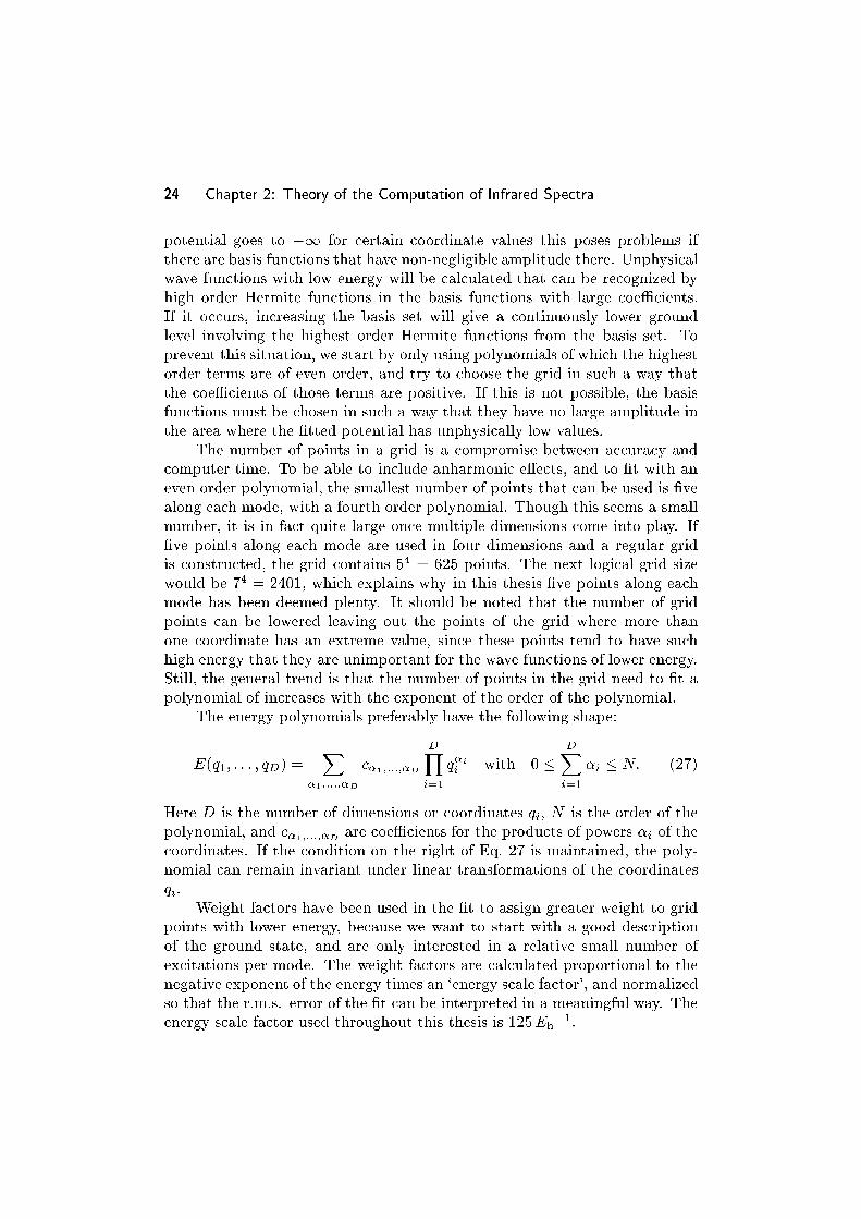
The energy polynomials preferably have the following shape:
E(q1; : : : ; qD) =X
�1;:::;�D
c�1;:::;�D
DYi=1
q�ii with 0 �
DXi=1
�i � N: (27)
Here D is the number of dimensions or coordinates qi, N is the order of the
polynomial, and c�1;:::;�D are coeÆcients for the products of powers �i of the
coordinates. If the condition on the right of Eq. 27 is maintained, the poly-
nomial can remain invariant under linear transformations of the coordinates
qi.
Weight factors have been used in the �t to assign greater weight to grid
points with lower energy, because we want to start with a good description
of the ground state, and are only interested in a relative small number of
excitations per mode. The weight factors are calculated proportional to the
negative exponent of the energy times an `energy scale factor', and normalized
so that the r.m.s. error of the �t can be interpreted in a meaningful way. The
energy scale factor used throughout this thesis is 125Eh�1.

Fitting the Potential Energy and Dipole Surfaces 25
2.2.2 Performing a Least Squares Fit with Singular Value Decomposition
Given the energy polynomial of Eq. 27, we have an equation for each energy
Ej calculated on the grid to �t the polynomial to:
Ej(q1j ; : : : ; qDj) =X
�1;:::;�D
c�1;:::;�D
DYi=1
q�iij ; j = 1; : : : ;M: (28)
Here qij is the value of coordinate qi for point j of the grid. The coeÆcients
c�1;:::;�D are the unknowns in these equations. If we suppose there are N
coeÆcients, and M grid points, we can write the equations in matrix form.
Qc = e (29)
Here Q is theM�N matrix containing the products of powers of coordinates
qi, c is the vector containing the coeÆcients c�1;:::;�D , and e is the vector
containing the energies from the grid points. The problem at hand is to �nd
a vector c such that r � jQc� ej is minimal, where r is called the `residual'.
This is the least squares approximation of the coeÆcients. If the number of
equations M is equal to the number of coeÆcients N , there exists a unique
solution with r = 0 to Eq. 29, provided there are no linear dependencies
between the equations. In practice, M and N are usually not equal and
you do not know in advance if the �t equations contain linear dependencies.
The method to tackle the situation is singular value decomposition. [3, and
references therein]
In linear algebra there exists a theorem that any M �N matrix A, with
N �M , can be decomposed into a column-orthonormal matrix U, a diagonal
matrix W, and the transpose of an orthonormal matrix V:
0BBBBB@
a11 � � � a1N...
...
ai1 � � � aiN...
...
aM1 � � � aMN
1CCCCCA =
0BBBBB@
u11 � � � u1N...
...
ui1 � � � uiN...
...
uM1 � � � uMN
1CCCCCA0@w1
. . .
wN
1A0@ v11 � � � vN1
.... . .
...
v1N � � � vNN
1A: (30)
26 Chapter 2: Theory of the Computation of Infrared Spectra
This decomposition can always be done, and is unique except for two trans-
formations: �rstly permutations of the columns of U, the elements ofW, and
the rows of VT ; secondly linear combinations of columns of U, and of rows of
VT whose corresponding elements of W are exactly equal.
If A is square and all elements of W are non-zero, it becomes easy to
compute the inverse of A with the singular value decomposition:
A�1 = V � [diag(1=wi)] �UT: (31)
This decomposition also shows when it becomes impossible to compute the
inverse of A, namely, if one of the singular values wi becomes zero. The con-
dition number of A is the ratio between the largest and the smallest element
of W. If this number becomes large, A becomes ill-conditioned. A condition
number is large if its reciprocal value is in the neighbourhood of the precision
of the computer you are working with, but there are more criteria. If the
condition number becomes in�nite, the matrix is singular.
SVD helps to �nd a useful answer to the equation Ax = b, even if A
is singular or ill-conditioned. The columns of U that correspond to non-zero
elements of W represent the range of A, whereas the columns of V that
correspond to elements of W that are zero span the null-space of A. If b lies
in the range of A, then the equations can be solved with SVD, replacing 1=wiwith 0 if wi = 0:
Ax = b ) x = V � [diag(1=wj)] � (UT � b): (32)
This yields the vector x with smallest length, and any linear combination of
the vectors from the null-space of A can be added to it. If b does not lie in
the range of A, then the equation cannot be solved, but x is the solution in
the least squares sense: the residual is minimized.
In practice, if there are elements of W that are very small compared
to the largest wi, 1=wi is also set to zero when computing x like in Eq. 32.
The reason is that these elements correspond to equations in Ax = b that
make large di�erences in x (1=wi is large), but contribute very little to the
improvement of the �t (i.e., the diminishing of the residual). The reason that
this is so can be numerical, but also inherent to the physical data. The best
way to get an idea for the limit below which to set 1=wi to zero is to order
the wi in decreasing size. Usually there is a gap of a few orders of magnitude
between the wi that are `OK', and those that should be zeroed. Like in the
choice of a grid and a basis set, there is a certain amount of Fingerspitzengef�uhl
involved.
Eq. 32, including zeroed 1=wi values, also applies to non-square matrices
A, where the number of equationsM is greater than the number of coeÆcients

Solving the Eigenvalue Problem with the Lanczos Method 27
N . In the case there are less equations than coeÆcients, the matrix A and
the vector b can be �lled up with zeroes until A is square. If this is done, or
indeed if any of the 1=wi need to be zeroed, the equations do not completely
determine the coeÆcients. In the application of SVD to the �t of a polynomial
to the potential energy grid, the �tted polynomial can still be used, and the
way it is obtained seems less arbitrary than leaving out certain coeÆcients
from the �t altogether.
SVD applied to Eq. 29 �nds the coeÆcients that minimize jQc�ej, whichcorresponds to an unweighted least squares �t. As mentioned earlier, the �ts
that are used in AnharmND are weighted. To get a properly weighted �t, we
apply SVD on
h[diag(
pw0
i)] �Qi� c =
h[diag(
pw0
i)] � ei; (33)
where w0
i are the �t weights (not to be confused with the singular values wi)
belonging to the energies Ei. The �t weights are calculated as
w0
i =e�f �EiPM
j=1 e�f �Ej
; (34)
where f is the energy scale factor mentioned earlier. For �t weights de�ned
in this way, the residual of Eq. 33 is the properly weighted r.m.s. error of the
�t on a grid point.
In AnharmND, the x, y, and z-component of the dipole are �tted to
polynomials as well, and the same weights are applied as for the �t of the
energy. However, it is possible to specify the dipole components for less grid
points than the energy, and then the weight factors are scaled so that the
r.m.s. error is still calculated per grid point where a dipole was given.
2.3 Solving the Eigenvalue Problem with the Lanczos Method
For the solution of the Schr�odinger equation, the lowest eigenvalues and eigen-
vectors of the Hamiltonian need to be computed. The Hamiltonian both sparse
and symmetric. Because of these properties, it is well suited to be tackled with
the Lanczos method.

28 Chapter 2: Theory of the Computation of Infrared Spectra
2.3.1 The Exact Lanczos Method
In its initial incarnation, the Lanczos method is a method to transform a
symmetrical matrix A of size n � n into a tridiagonal form T, with a trans-
formation matrix Y � [y1 y2 : : : yn], where fyig form an orthonormal set of
vectors. The eigenvalues and vectors of a tridiagonal matrix can be computed
readily.
AY = YT = [y1 y2 : : : yn]
266666664
�1 �2
�2 �2 �3
�3 �3 �4
�4
. . .. . .
. . .. . . �n
�n �n
377777775
(35)
Paige [4] found two numerically stable algorithms to compute the vectors
yi and the tridiagonal matrix T to �nd eigenvalues. We use the following
algorithm. Take a random vector y1 of unit length, let �1 = 0, and for i = 1
to n, do
1. v Ayi.
2. �i yTi v.
3. z v � �iyi � �iyi�1.4. �i+1
pzTz.
5. if �i+1 = 0, then stop; otherwise, yi+1 z=�i+1 and continue.
(36)
It can be shown that, for exact arithmetic, the vectors yi form an orthonormal
set. In exact arithmetic, the algorithm stops if �i+1 equals 0. This can happen
at �i+1 if y1 is orthogonal to n � i eigenvalues of A. If �i+1 = 0 and i < n
then Yi = [y1 y2 : : : yi] is an invariant subspace, and the algorithm can
be continued with a vector yi+1 that is orthogonal to all y1; : : : ;yi. The
algorithm has to end with �n+1 = 0 because you cannot have more than n
orthogonal vectors of size n.
After the construction of the tridiagonal matrix T, its eigenvalues �iwith eigenvectors ti can be computed. The eigenvalues �i of the symmetrical
matrixA are identical to those of T, and the eigenvectors ai can be calculated
if the Lanczos vectors yi have been stored, by ai = Yti.

Solving the Eigenvalue Problem with the Lanczos Method 29
2.3.2 The Blessing of Round-O� Errors in Lanczos
In exact arithmetic the Lanczos vectors that are generated in the Lanczos
procedure are all orthogonal, but in �nite accuracy calculations such as they
occur in computers, they are not. In the procedure outlined in the previ-
ous paragraph, yi is orthogonalised explicitly only to yi�1 and to yi�2. The
implicit orthogonality with respect to the other yi is gradually lost after a
number of iterations. As a result the matrix T will not have exactly the same
eigenvalues as A, and the eigenvectors of A are not exactly reproduced by
Yti. Originally, Lanczos tried to �x the method by reorthogonalisation of the
vectors yi against all previous ones. This works, but the associated computa-
tional cost is prohibitive for large matrices A, both in terms of memory and
CPU usage.
Paige showed that for large numbers of iterations, a good number of the
extreme eigenvalues of A can be found. If the number of iterations exceeds
the dimension n of A, a few conceptual problems appear. They are related to
the fact that YTi AYi has a greater dimension than A. This means that more
eigenvalues can be computed from T than A actually has, some of which are
multiple copies of eigenvalues that A has, others which are not eigenvalues
of A at all. These super uous eigenvalues are called `spurious multiplicities'
and `spurious eigenvalues' respectively, and a practical implementation of the
Lanczos method needs a test to distinguish them from `genuine' eigenvalues.
The test we applied will be discussed further on. Spurious multiplicities and
eigenvalues already appear in the case that the number of iterations does not
exceed the dimension of A.
Although it seems an annoying complication at �rst sight, the loss of
orthogonality in the Lanczos method with �nite accuracy is the very reason
it works in practice. The Lanczos method only �nds eigenvectors that are
in the part of the eigenspace spanned by Yi. In exact arithmetic this means
that y1 must be a linear combination of all eigenvectors of A to continue the
iteration to Yn without getting �i+1 = 0 before the complete vector space
is spanned. This is a tough call on a randomly chosen vector. In the �nite
accuracy practice of computers the event that �i+1 becomes zero is extremely
rare. If �i+1 in the procedure given in the previous section becomes small,
rounding errors in z in step 5 are transferred much in ated into yi+1. This
is where loss of orthogonality is introduced, but with it may also come parts
of the eigenvector space not yet present in y1. If enough Lanczos iterations
are carried out, a good number of extreme eigenvalues are found, even if
the corresponding eigenvectors ai are orthogonal to the �rst random Lanczos
vector.

30 Chapter 2: Theory of the Computation of Infrared Spectra
If loss of orthogonality is severe, the correspondence between the eigen-
values of T and A will be poor whereas if the columns of Y are perfectly or-
thogonal, there is the risk of missing out part of the eigenspace of A. Lewis [5]
recommends partial reorthogonalisation of vectors yi against yi�1 and yi�1.
This appears to provide enough orthogonality to obtain more eigenvalues than
just the most extreme ones. The procedure then becomes
1. v Ayi.
2. �i yTi v.
3. z v � �iyi � �iyi�1.4. z z� (zTyi)yi:
5. z z� (zTyi�1)yi�1:
6. �i+1 pzTz.
7. if �i+1 = 0, then stop; otherwise, yi+1 z=�i+1 and continue.
(37)
In the computer version of the algorithm, if �i+1 = 0, the procedure is sim-
ply restarted with a di�erent random starting vector. In practice this never
happens.
2.3.3 Getting Rid of Spurious Eigenpairs
We compute infrared absorption intensities and expectation values of coordi-
nates. Both properties can be computed straightforwardly using the eigen-
vectors of the Hamiltonian. If the eigenvectors are going to be computed
anyway, there is a convenient way to compute the accuracy of the eigenvalues.
In Dirac notation, if there is a normalized vector j i with an expectation valueh jHj i, then there exists an eigenvalue � of the operator H such that [6]
jh jHj i � �j �ph jH2j i � jh jHj ij2: (38)
This expression provides a way to discover spurious eigenvalues: if the in-
terval computed for a vector j i is too wide, it is not a good approximation
of an eigenvector. Spurious multiplicities are found by orthogonalisation of
eigenvectors of the tridiagonal matrix that have overlapping intervals contain-
ing eigenvalues of the Hamiltonian. If the orthogonalisation makes a vector
vanish, it counts as a spurious multiplicity.

Solving the Eigenvalue Problem with the Lanczos Method 31
2.3.4 A Modi�ed Lanczos Procedure
For some of the infrared spectra we have computed, we need so many eigen-
values and vectors that the number of Lanczos iterations necessary to �nd
them becomes prohibitive in terms of computation time and use of memory,
especially because we want to �nd the eigenvectors as well as the eigenval-
ues. There are two properties that make an eigenvector likely to be found in
a Lanczos procedure: being at the extremes of the eigenspectrum, and be-
ing well separated from other eigenvalues. We used a method that aims at
improving the separation of the eigenvalues we search, at the expense of the
eigenvalues we are not interested in. In this procedure which is described by
Lewis [5], the original Hamiltonian H is replaced with a polynomial of this
Hamiltonian f(H). The function f modi�es the eigenspectrum of H, whereas
the eigenvectors of f(H) are the same as those of H.
For the construction of f we �rst determine the extreme eigenvalues of
the Hamiltonian H. This can be done easily with a standard Lanczos pro-
cedure. Once we know the interval [Emin; Emax] in which the eigenvalues lie,
we choose a value E0 2 [Emin; Emax] that is an upper limit for eigenvalues
we want to compute. Then we construct a polynomial that `folds up' the
interval [E0; Emax], and stretches the interval [Emin; E0], such as fourth order
polynomial in the following graph:
fmax
f0
fmin
Emin E0 Emax
The interval [f(Emin); f(E0)] has much better separated eigenvalues compared
to [f(E0); f(Emax)], than the interval [Emin; E0] has compared to [E0; Emax].
Eigenvalues of H can be computed as expectation values of the eigenvectors
found for f(H), and tested for accuracy in the same way as in the plain
Lanczos procedure. Using this modi�cation it appears possible to obtain
higher eigenvalues in less iterations.

32 Chapter 2: Theory of the Computation of Infrared Spectra
2.4 Infrared Absorption Intensities
2.4.1 The Law of Lambert and Beer, Integrated Absorption Intensities
The law of Lambert and Beer describes the absorption of radiative energy in
a medium:
I(�) = I0 e�k(�)�x
: (39)
I0 in this formula denotes the initial intensity, I(�) the intensity at frequency
�, k(�) the absorption coeÆcient for frequency (�), and x is a quantity denot-
ing the number of absorbing molecules per unit surface area. The quantity x
has been de�ned in disturbingly many di�erent ways.[7] It is the product of a
concentration and a length, and for both quantities di�erent units are being
used. AnharmND uses
x � n � l; (40)
where n is the concentration in mol/m3, and l is a length the radiation travels
through, in m. The absorption coeÆcient k(�) can be written as follows:
k(�) = S f(� � �0): (41)
Here S is the integrated absorption coeÆcient, also called line strength or
line intensity, and f(� � �0) is a function describing the line shape, that is
normalised by the requirement
Z1
�1
f(� � �0)d� = 1: (42)
From Eq. 41 and 42, we �nd that
S =
Z1
�1
k(�)d�: (43)
This expression shows us that the units in which S is expressed are the units of
� divided by the units of x. AnharmND uses the same convention as quantum
chemical programs such as Gaussian, where � is in wave numbers. As a result,
S is expressed in km=mol.

Infrared Absorption Intensities 33
2.4.2 Einstein CoeÆcients
Einstein has established the relationship between absorption and emission of
radiation of a system with two states in a radiation bath in thermal equilib-
rium.[8] From his analysis we get the de�nitions of the so-called Einstein A
and B coeÆcients.
Assume a system that has two stationary states with energiesEm and En,
where Em > En. Absorption of radiation with frequency �nm will bring the
system from state n to m. The frequency �nm follows from Bohr's frequency
rule:
�nm =Em �En
h
: (44)
The radiative density is given by �(�), where �(�)d� is the energy of radiation
with frequency between � and � + d�. The probability of the system in state
n to absorb a quantum in a unit of time is given by
Bn!m�(�nm); (45)
where Bn!m is the Einstein coeÆcient of absorption. Einstein has shown that
the probability of emission should be divided into two parts: spontaneous and
stimulated emission. The probability for the system in state m to emit a
quantum per unit time is given by
Am!n +Bm!n�(�nm); (46)
where Am!n is Einstein's coeÆcient of spontaneous emission, and Bm!n is
the Einstein coeÆcient of stimulated emission.
Consider a large number of systems in equilibrium with radiation at tem-
perature T . According to Planck,[8] the distribution of radiation is given
by
�(�) =8�h�3
c3
(eh�=kT � 1)�1: (47)
Assume Nn systems in state n, and Nm systems in state m. At equilibrium
the number of transitions from n to m, NnBn!m�(�nm), and the number
of transitions from m to n, Nm[Am!n +Bm!n�(�nm)], are equal. From this
equality an expression can be derived for the ratio between Nn and Nm, which
can then be equated to the ratio according to the Boltzmann distribution:
Nn
Nm
=Am!n + Bm!n�(�nm)
Bn!m�(�nm)= e
�(En�Em)=kT = eh�nm=kT
: (48)
This expression can be rewritten as
�(�nm) =Am!n
Bn!meh�nm=kT �Bm!n
: (49)

34 Chapter 2: Theory of the Computation of Infrared Spectra
To match this with Planck's law, the following two requirements arise:
Bn!m = Bm!n
Am!n =8�h�3nmc3
Bm!n:
(50)
2.4.3 Time Dependent Perturbation Theory
To compute the transition probability for a system from one state to another
in quantum mechanics, we apply time dependent perturbation theory.[9] The
time dependent Schr�odinger equation is given by
Hji = i�h@
@t
ji: (51)
If the Hamiltonian H does not depend on time, it can be solved by separation
of variables:
ji = j ie�iEt=�h; (52)
where j i is the solution to the time-independent Schr�odinger equation
Hj i = Ej i: (53)
Consider a system with orthonormal states j ji that are eigenstates of the
time-independent Hamiltonian H0. Any state of the system can be expressed
as a linear combination of these states, e.g.
jit=0 =Xj
cj j ji (54)
or, more general,
ji =Xj
cj j jie�iEjt=�h (55)
Normalization of ji requires thatXj
jcj j2 = 1: (56)
Since the states j ji form a complete set, Eq. 55 still holds when a time de-
pendent perturbationH 0 is added to the Hamiltonian, with the di�erence that
the formerly constant coeÆcients cj now become functions of time. For this
reason time-dependent perturbation theory is sometimes called the `method
of variation of constants'. If we start with cn(0) = 1 and cm(0) = 0 for m 6= n,
Infrared Absorption Intensities 35
and at some later time t1 we have cn(t1) = 0 and jcm(t1)j2 = 1, we say that
the system underwent a transition from j ni to j mi.To �nd cn(t) and cm(t), we require that ji from Eq. 55 satisfy the time
dependent Schr�odinger equation with Hamiltonian H0 +H0.
Xj
cj [H0j ji]e�iEjt=�h +Xj
cj [H0j ji]e�iEjt=�h =
Xj
i�h _cj j jie�iEjt=�h +Xj
i�hcj@
@t
�j jie�iEjt=�h
� (57)
The �rst and the last sum in this equation cancel because j ji are eigenfunc-tions of H0, so that we getX
j
cj [H0j ji]e�iEjt=�h =
Xj
i�h _cj j jie�iEjt=�h (58)
Separate expressions for each _ck can be obtained by taking the inner product
of Eq. 58 with h kj
Xj
cjh kjH 0j jie�iEjt=�h = i�h _cke�iEkt=�h (59)
We de�ne the following shorthand:
H0
ab � h ajH0j bi (60)
Eq. 59 can be rewritten as
_ck = �i
�h
hckH
0
kk +Xj 6=k
cjH0
kje�i(Ej�Ek)t=�h
i: (61)
Typically the diagonal matrix elements of H 0 are zero, which gives the follow-
ing equation for each _ck:
_ck = �i
�h
Xj 6=k
H0
kje�2�i�kjt
cj ; (62)
where �kj is de�ned as in Eq. 44.
In perturbation theory, equations 62 are solved by successive approxi-
mations, assuming that H 0 is small. Consider the system starts in the lower
36 Chapter 2: Theory of the Computation of Infrared Spectra
state j ni. In the absence of a perturbation, the system would stay like this
forever. This is the zeroth order approximation:
c(0)n (t) = 1; c
(0)
m6=n(t) = 0: (63)
We get the �rst order approximation inserting these values in Eq. 62 (taking
k = n, and k = m, respectively):
dcn
dt
= 0 ) c(1)n (t) = 1
dcm
dt
= �i
�hH
0
mne2�i�nmt ) c
(1)m (t) = �
i
�h
Z t
0
H0
mn(t0)e2�i�nmt
0
dt0
(64)
Obviously, c(1)n (t) and c
(1)m (t) do not ful�ll the normalization condition Eq. 56.
This is because they are only correct to �rst order. The second order ap-
proximation can be obtained inserting c(1)n (t) and c
(1)m (t) into the right hand
side of Eq. 62. This will give a new expression for c(2)n (t), but the expression
for c(2)m (t) will be identical to the one for c
(1)m (t). Since we are interested in
the development of cm(t), the �rst order approximation gives a useful result
already, that is in fact correct to second order.
2.4.4 Quantum Mechanical Calculation of the Einstein CoeÆcients
With the aid of time dependent perturbation theory, and a classical treatment
of the electromagnetic �eld, an expression can be derived for the Einstein
coeÆcients.
In classical electrodynamics, an electromagnetic wave consist of trans-
verse and mutually perpendicular electric and magnetic �elds. Atoms and
molecules interact primarily with the electric component of such waves. For
visible and infrared light the wave length is several orders of magnitude larger
than the molecular dimensions, so that the electric �eld can be considered
constant in space, but varying in time:
E = E0 cos(2��t)k: (65)
Here E is the electric �eld with frequency �, amplitude E0, and polarisation
vector k of unit length. If we assume that E is polarised in the z-direction,
the perturbing Hamiltonian H 0 is given by
H0 =
Xj
QjE0zj cos(2��t) = �zE0 cos(2��t); (66)
Infrared Absorption Intensities 37
where Qj are the charges in the system with z-coordinate zj , and �z is the
z-component of the dipole moment.
Before we proceed inserting this expression in Eq. 64, we need to re-
address the diagonal elements H 0
kk in Eq. 59 and 61. If the described system
is an atom, the wave functions j ki are usually either even or odd functions
of z, and �z is an odd function of z. This causes diagonal matrix elements
of H 0 to vanish. In this thesis j ki usually represents a vibrational wave
function that often is not purely even or odd, and �z often contains a constant
term. If the diagonal terms are not set to zero, this changes the �rst order
approximation of cn(t), but the c(1)m (t) remains the same as in Eq. 64. Since
we are interested in cm(t), we can continue to use Eq. 64 as the �rst order
approximation of cm(t), but it can no longer be regarded as correct to second
order for all vibrational modes.
A matrix element of H 0 can be split in a time dependent and a time
independent part:
H0
ab = h aj�zE0 cos(2��t)j bi = E0h aj�zj bi cos(2��t) = Vab cos(2��t);
where Vab � E0h aj�zj bi:(67)
We can insert this into the expression for c(1)m (t) from Eq. 64, to get
cm(t) � �iVmn
�h
Z t
0
cos(2��t0)e2�i�nmt0
dt0
= �iVmn
2�h
Z t
0
he2�i(�nm+�)t0 + e
2�i(�nm��)t0
idt0
= �Vmn
4��h
�e2�i(�nm+�)t � 1
�nm + �
+e2�i(�nm��)t � 1
�nm � �
�:
(68)
This expression can be simpli�ed because we are mainly interested in fre-
quencies � in the neighbourhood of �nm, and frequencies far from that value
are not likely to cause a transition anyway. This means that the left term be-
tween the brackets in Eq. 68 becomes negligible compared to the right term,
and it can be dropped:
cm(t) � �Vmn
4��h
�e�i(�nm��)t � e��i(�nm��)t
�nm � �
�e�i(�nm��)t
= �iVmn
2��h
sin(�(�nm � �)t)�nm � �
e�i(�nm��)t
:
(69)
38 Chapter 2: Theory of the Computation of Infrared Spectra
From this we �nd that the probability Pn!m to �nd the system in j mi attime t, if it was in j ni at time t = 0, under the in uence of an electric �eld
polarised in the z direction, is given by
Pn!m(t) = jcm(t)j2 �jVmnj2
4�2�h2sin2[�(�nm � �)t]
(�nm � �)2
=E20 jh mj�z j nij2
4�2�h2sin2[�(�nm � �)t]
(�nm � �)2:
(70)
In classical electrodynamics, the energy per unit volume u in electromag-
netic �elds is given by
u =�0
2E2 +
1
2�0B2; (71)
where E and B are the electric and magnetic �elds, �0 is the electric per-
mittivity of vacuum, and �0 is the magnetic permeability of vacuum. For
electromagnetic waves the electric and magnetic contributions are equal. On
the average over a cycle the energy in an electromagnetic wave is then given
by
u =�0
2E20 : (72)
This means that the transition probability from Eq. 70 is proportional to the
energy density of the �elds:
Pn!m(t) =ujh mj�z j nij2
2�2�0�h2
sin2[�(�nm � �)t](�nm � �)2
: (73)
This holds for a monochromatic perturbation, of frequency �. In realistic
situations the system is exposed to electromagnetic waves in a range of fre-
quencies. This means that we need to replace u with an energy density �(�)d�
in the range d�, and integrate over �:
Pn!m(t) =jh mj�zj nij2
2�2�0�h2
Z1
0
�(�)
�sin2[�(�nm � �)t]
(�nm � �)2
�d�: (74)
The term in curly braces in Eq. 74 has a sharp peak around � = �nm, whereas
�(�) in general is a much broader function (Eq. 47), so we can approximate
�(�) with �(�nm):
Pn!m(t) �jh mj�zj nij2
2�2�0�h2
�(�nm)
Z1
0
�sin2[�(�nm � �)t]
(�nm � �)2
�d�: (75)

Infrared Absorption Intensities 39
The integration range in Eq. 75 can be extended to �1 : : :1, because the
function only has non-negligible value around � = �nm. Then after substitu-
tion of x � �(�nm � �)t, and using
Z1
�1
sin2 x
x2dx = �; (76)
we get
Pn!m(t) �jh mj�z j nij2
2�0�h2
�(�nm)t: (77)
From this we can calculate the transition rate Rz for polarised light along the
z-axis as
Rzn!m =
dPn!m
dt
=jh mj�zj nij2
2�0�h2
�(�nm): (78)
This expression holds if the dipole moment of the system and the polarisation
of the electric �eld are both in the same direction. For the general case we need
to replace jVnmj2 in Eq. 70 by E20 jh mj�j nij2 � (k �m)2 where the orientation
factor (k �m)2 is the square of the inner product of the polarisation direction
k of the electric �eld with the direction of the dipole moment m, averaged
over all possible relative orientations. Both k and m have unit length. The
orientation factor can be computed by
(k �m)2 =
R 2�0
d�
R �0d� cos2 � sin �R 2�
0d�
R �0d� sin �
=1
3: (79)
This expression is found taking � as the angle between k and m, and � the
rotation angle of m around k at �xed �. For given values of � and � the
square of the inner product is then cos2 �. With this result we can rewrite
Eq. 78 for the transition rate Rn!m for the system in any orientation with
electromagnetic radiation coming from all directions:
Rn!m =jh mj�j nij2
6�0�h2
�(�nm): (80)
By comparison of this expression with Eq. 45 we �nd the expression for the
Einstein coeÆcient of absorption:
Bn!m =jh mj�j nij2
6�0�h2
: (81)

40 Chapter 2: Theory of the Computation of Infrared Spectra
2.4.5 Calculation of the Integrated Absorption CoeÆcient
We need to make a connection between Einstein CoeÆcients and measurable
quantities.[10] Assume a beam of radiation with intensity I shines on a con-
tainer with our system with two states j ni and j mi. The di�erential changein intensity can be given by
�dI = h�nmBn!m�(�nm)Nndl; (82)
where Bn!m�(�nm) is the number of transitions per second of one system in
the presence of radiation energy density �(�nm) (see Eq. 45), h�nm the energy
absorbed by one transition, Nn the number of particles in state j ni per unitvolume, and dl the distance traveled through the sample.
The relationship between the energy ux or intensity I and the radiation
energy density �(�) is given by
I =
Zc�(�)d�; (83)
where c is the speed of light. For the frequencies around �nm that are of im-
portance for the transition we are studying, �(�) can be regarded as constant
(compare Eq. 75). This means that in that frequency range I(�) can also be
regarded as constant, and we get
I(�nm) = c�(�nm)��; (84)
where �� is the width of the peak. This can be substituted in Eq. 82, to give
�dI =h�nm
c��Bn!mI(�nm)Nndl: (85)
Compare this to the di�erential form of Eq. 39:
�dI = k(�)I(�)ndl: (86)
This gives
k(�)�� �NAh�nm
c
Bn!m (87)
where Avogadro's number NA appears because the units of n are mol/m3 and
those of Nn are molecules per m3. This equation is approximate because k(�)
is not constant over the width of the peak. Since in the calculation of the Ein-
stein coeÆcient the frequency dependency has been integrated out (Eq. 75), it
follows that the same should be done with the absorption coeÆcient, so thatZk(�)d� =
NAh�nm
c
Bn!m: (88)

Infrared Absorption Intensities 41
In practice, the integration is usually not carried out over frequency �, but over
wave numbers �=c. This means that for the integrated absorption coeÆcient
S in m/mol we have the following quantum mechanical expression:
Sn!m =
Zk(�)
c
d� =NAh�nm
c2
Bn!m =2�2NA�E
3�0h2c2jh mj�j nij2; (89)
where �E is the energy di�erence between j mi and j ni. For absorption
spectra of multiple levels at higher temperatures than 0K, a Boltzmann dis-
tribution factor is added to account for occupation of levels higher than the
ground state:
S(T )n!m =2�2NA�E
3�0h2c2jh mj�j nij2
e�En=kTPMj e
�Ej=kT: (90)
In this expression M is the number of states, and Ej is the energy of j ji.Eq. 90 has been used throughout this thesis in the computation of infrared
spectra. It disregards the e�ects of stimulated emission, that are proportional
to the occupation of the excited level involved in a transition. The e�ect of
induced emission can be accounted for subtracting a term from the Boltzmann
distribution factor, so that it becomes
e�En=kT � e�Em=kTPM
j e�Ej=kT
: (91)
This means that all intensities in the spectra could be corrected if they were
multiplied by the factor
e�En=kT � e�Em=kT
e�En=kT
= 1� e��E=kT (92)
At a temperature of 298.15K this factor as a function of wave numbers looks
like this:
0
0.99
0 2000
inte
nsity
rat
io
wave number (1/cm)
Influence of Induced Emission on Intensity at 298.15K
144 477 954
0.50
0.90
42 Chapter 2: Theory of the Computation of Infrared Spectra
The correction diminishes the intensity by a factor of 0.5 at 144 cm�1, 0.9
at 477 cm�1, and 0.99 at 954 cm�1. The most interesting transitions of the
spectra in this thesis are in the region where the e�ect of induced emission
can be neglected.
References
[1] B. Podolsky; Phys. Rev., \Quantum-Mechanically Correct Form of Ha-
miltonian Function for Conservative Systems", 32, 812{816 (1928).
[2] A. Messiah; Quantum Mechanics; chap. XII, North Holland, Amsterdam,
1962.
[3] W. H. Press, S. A. Teukolsky, and W. T. Vetterling; Numerical recipes in
C : the art of scienti�c computing; chap. 2.9, 14.3, Cambridge University
Press, Cambridge, 1992.
[4] C. C. Paige; J. Inst.Maths. Appl., \Computational Variants of the Lanc-
zos Method for the Eigenproblem", 10, 373{381 (1972).
[5] J. G. Lewis; Algorithms for sparse matrix eigenvalue problems; Stanford
University, Department Computer Science, Stanford, 1977.
[6] B. N. Parlett; The Symmetric Eigenvalue Problem; Prentice-Hall, Engle-
wood Cli�s, 1980.
[7] K. Narahari Rao; (editor)Molecular Spectroscopy: Modern Research, vol.
2; chap. 4 by L. A. Pugh, and K. Nahari Rao; \Intensities from Infrared
Spectra", Academic Press, London, 1976.
[8] L. Pauling, and E. B. Wilson Jr.; Introduction to quantum mechanics
with applications to chemistry; chap. XI-40a, McGraw-Hill, London, 1935.
[9] D. J. GriÆths; Introduction to Quantum Mechanics; chap. 9, Prentice
Hall, Englewood Cli�s, 1995.
[10] E. B. Wilson Jr., J. C. Decius, and P. C. Cross; Molecular Vibra-
tions: The Theory of Infrared and Raman Vibrational Spectra; chap. 7-9,
McGraw-Hill, London, 1955.

3Three and Four-Coordinate Cluster Models
Abstract
The in uence of acetonitrile adsorption on the infrared spectrum of an acidic
OH group inside a zeolite is studied by theoretical calculations. The zeolite
is modelled by a cluster molecule. Potential energy and dipole surfaces of
the stretch and two bending coordinates of the acidic H atom, and, for the
complex with acetonitrile, of an additional acetonitrile stretch coordinate,
are computed employing Hartree-Fock as well as density functional methods.
Infrared frequencies as well as absorption intensities are computed taking into
account mechanical as well as electric anharmonicities up to fourth order.
Fermi resonance proposed as cause of the splitting of OH stretch absorption
bands in infrared spectra is explicitly considered.
Reproduced in part with permission from E.L. Meijer, R.A. van Santen, and
A.P.J. Jansen: \Computation of the Infrared Spectrum of an Acidic Zeolite
Proton Interacting with Acetonitrile", J. Phys. Chem. 100 9282{9291 (1996).
Copyright 1996 American Chemical Society.

44 Chapter 3: Three and Four-Coordinate Cluster Models
3.1 Introduction
The infrared spectrum of an XH group in a molecule, where X is typically one
of O, S, F, Cl, Br, or I, can change radically upon hydrogen bonding to some
base B. In many di�erent systems the following changes are observed. The
XH stretching frequency is lowered considerably, the absorption intensity of
the band is enhanced greatly, and the band is broadened by a large amount.
In a number of cases the hydrogen bonded XH stretch band is split into two
or more bands. All of the described phenomena appear to be stronger if the
acidity of the XH group is greater, or if the basic character of B is stronger.
The system under study in the present work is a Br�nsted acidic OH
group of a zeolite interacting with a molecule of acetonitrile. This system is
especially interesting because it exhibits a very large OH stretch frequency
shift, and also the splitting of the shifted OH stretch band. In the case of
adsorption of methanol in a zeolite, a similar multiple band structure has
been found. Kubelkov�a et al.[1] have argued the two bands around 2400 cm�1
and 2900 cm�1 were due to two di�erent structures, in one of which the proton
is transferred to the methanol, and in the other it is not. The same bands
have been interpreted by Mirth et al. [2] as originating from a symmetric and
an asymmetric bending of the two hydrogen atoms of the protonated hydroxyl
group of methanol. Obviously, this explanation cannot be used for the similar
bands of a Br�nsted acidic zeolite with acetonitrile around 2400 cm�1 and
2800 cm�1. In liquids broadening of the XH stretch bands upon hydrogen
bonding has been explained from the coupling with XH� � �B intermolecular
stretch modes.[3{5] Splitting of the XH stretch bands has been explained
by Fermi resonances of overtones of XH bending modes.[3, 5] Based on a
comparison of the in-plane bending modes of an acidic OH group in a zeolite
and peak minima in the infrared spectrum, Pelmenschikov et al. [6] proposed
a Fermi resonance of the downwards shifted OH stretch mode and the upwards
shifted in-plane bending overtone.
In order to examine these models in more detail, in the current paper
we present calculations of vibrational frequencies and infrared absorption in-
tensities including anharmonicities. Vibrational wave functions are computed
for the stretch and bending modes of an acidic proton in a zeolite, and of
such a proton with an adsorbed molecule of acetonitrile, where the coupling
of the proton modes with the stretch mode of the acetonitrile molecule as a
whole with respect to the OH group was included. Anharmonic terms up to
fourth order in the potential energy were included, and infrared absorption
intensities were computed using a fourth-order dipole surface. The vibrational
wave functions were computed in a variational approach. The potential en-
ergy and dipole surfaces were �tted to quantum chemical calculations using
polynomials.
Theory 45
3.2 Theory
3.2.1 The Potential Energy and Dipole Surfaces
The computation of the potential energy and dipole surfaces has been done
at the Hartree-Fock level of theory (SCF), and also using density functional
theory (DFT). The density functional applied was Becke's 3 parameter func-
tional with the non-local correlation provided by the Lee, Yang, and Parr
expression.[7{10] DFT is assumed to yield results that are closer to experi-
ment, for the energy as well as for the dipole surface.[11] Since the computed
infrared spectra from the SCF data and the DFT data were qualitatively very
similar, the DFT results are presented completely, and only in some cases
supplemented by the SCF results.
The cluster approach has been used to model the acidic site of the zeolite.
We have used a relatively small cluster, to allow for electronic structure cal-
culations with a reasonably good basis set. The cluster contained the acidic
Al(OH)Si group with the dangling bonds of Al and Si saturated by OH groups.
A restricted geometry optimisation has been done for this cluster, with and
without an interacting molecule of acetonitrile, to obtain reference points for
the potential energy and dipole surfaces. Full optimisation of the geometry of
the cluster was not done for two reasons.
Firstly, the cluster molecule forms internal hydrogen bridges between
the terminating OH groups. These hydrogen bridges a�ect the (Al{O{Si)
angle, and hence the OH-frequency, in a way that is not found in zeolite
systems, which we attempt to model. To prevent internal hydrogen bridging,
we have optimised the zeolite cluster without acetonitrile with the (Si{O{H)
and (Al{O{H) angles of the terminatingOH groups �xed at tetrahedral angles,
and required that, going from the central O atom to a terminal OH, the atoms
O{T{O{H (T=Si or T=Al), should be in one plane.
The second reason not to optimise fully has been computational cost. We
have imposed Cs symmetry, with the Al(OH)Si part of the cluster positioned
in the mirror plane. This has allowed for a considerable reduction of the
number of points to be computed for the potential energy surface, as both
sides of the mirror plane are equivalent.
In the optimisation of the geometry of the zeolite cluster interacting with
acetonitrile, we have �xed the terminal OH groups to the positions found in
the optimisation of the free zeolite cluster, attempting to model the `rigidity'
of the zeolite lattice. The acetonitrile has been positioned with the CN group
pointing towards the acid OH group, as shown in Fig. 1.
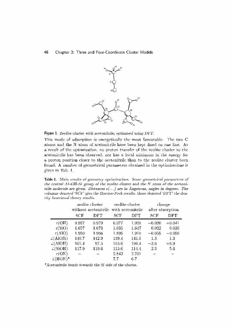
46 Chapter 3: Three and Four-Coordinate Cluster Models
O
O
O
O
OO
H
HH
H
HH
AlO
Si
H
N
C
C
HH H
Figure 1. Zeolite cluster with acetonitrile, optimised using DFT.
This mode of adsorption is energetically the most favourable. The two C
atoms and the N atom of acetonitrile have been kept �xed on one line. As
a result of the optimisation, no proton transfer of the zeolite cluster to the
acetonitrile has been observed, nor has a local minimum in the energy for
a proton position closer to the acetonitrile than to the zeolite cluster been
found. A number of geometrical parameters obtained in the optimisations is
given in Tab. 1.
Table 1. Main results of geometry optimisations. Some geometrical parameters of
the central Al{OH{Si group of the zeolite cluster and the N atom of the acetoni-
trile molecule are given. Distances r(: : :) are in �Angstrom, angles in degrees. The
columns denoted `SCF' give the Hartree-Fock results, those denoted `DFT' the den-
sity functional theory results.
zeolite cluster zeolite cluster change
without acetonitrile with acetonitrile after absorption
SCF DFT SCF DFT SCF DFT
r(OH) 0:957 0:979 0:977 1:020 +0:020 +0:041
r(SiO) 1:657 1:673 1:635 1:647 �0:022 �0:026r(AlO) 1:950 1:966 1:895 1:910 �0:055 �0:056
6 (AlOSi) 140:7 142:9 139:4 141:6 �1:3 �1:36 (AlOH) 101:4 97:5 105:0 104:4 +3:6 +6:96 (SiOH) 117:9 119:6 115:6 114:4 �2:3 �5:6r(ON) { { 2:843 2:701 { {
6 (HON)* { { 7:7 6:7 { {
*Acetonitrile bends towards the Si side of the cluster.
Theory 47
The basis used to compute the potential energy surface has been chosen so
as to give a good description of the near environment of the acidic H atom. At
the borders of the zeolite cluster a minimal basis set has been used to reduce
computational cost. A STO-3G basis set[12] has been used for the H atoms of
the terminating OH groups. We have used a 6-31G** basis set[13{16] for the
O atoms of the terminating OH groups, for Si, Al, the acidic H of the zeolite
cluster, and for the C and H atoms of the acetonitrile. For the central O atom
of the zeolite cluster and the N atom of acetonitrile, a 6-311+G* basis set
has been employed, that provides a good description of the proton aÆnity of
anions.[17{19] From the results in [19], the proton transfer from H2O to NH3
can be computed to become less unfavourable when going from a double to a
triple zeta basis set, and adding di�use functions. This e�ect can be ascribed
to the better description of anionic oxygen. Since the interaction between the
acidic OH and acetonitrile under study in the current article resembles the
beginning of a proton transfer from an oxygen atom to a nitrogen atom, we
expect that the used basis set will result in a stronger calculated interaction.
Further on in the paper it will be shown that yet a stronger interaction is
needed to account for the experimentally observed spectra.
Recently, Haw et al.[20] have done a number of SCF geometry optimisa-
tions where the acetonitrile molecule has been forced at a more acute angle
with the acidic OH in order to model the spatial limitations within a zeolite.
We do not feel that changing this angle would have any essential in uence on
our current results, because the potential of the bending of the acetonitrile
molecule as a whole is rather at.
The potential energy and dipole surfaces of the zeolite cluster without
acetonitrile adsorbed have been computed as a function of the acidic H posi-
tion. The grid we have used to compute potential energy and dipole surfaces
has been designed to cover the area in coordinate space where the vibrational
wave functions have non-negligible amplitude, i.e., where the potential energy
is relatively low. This leads to a description where the grid is closer spaced in
areas where the potential energy is changing strongly in a certain direction,
e.g., for shorter OH distances. The energy and dipole have been computed at
�ve di�erent OH distances: 0.8, 0.9, 1.0, 1.1, and 1.4 times the equilibrium
distance listed in Tab. 1. For each of these OH distances, the H atom was
bent towards the Al atom by an angle � of 0Æ, 7.5Æ, 20Æ, and 60Æ, and sub-
sequently rotated around the axis de�ned by the equilibrium OH bond by an
angle � of 0Æ, 45Æ, 90Æ, 135Æ, and 180Æ. The number of points for which an
electronic structure calculation has been done is 80. The values of 45 points
corresponding to angles � of 225Æ, 270Æ, and 315Æ, have been derived taking
the symmetry plane of the cluster into account, adding up to a total of 125
points.
48 Chapter 3: Three and Four-Coordinate Cluster Models
The energy and dipole surfaces of the zeolite cluster with acetonitrile
adsorbed have been scanned in the same way as those of the `bare' zeolite
cluster with respect to the H positions. For each of the 80 hydrogen positions,
energy and dipole have been computed at �ve di�erent acetonitrile positions.
The acetonitrile molecule has been moved as a whole along its N�C{C axis
found in the equilibrium geometry, with O{N distances of the equilibrium
value listed in Tab. 1, and the equilibrium value plus and minus 0.15 �A, and
plus and minus 0.5 �A. The total number of points for which an electronic
structure calculation has been done for this complex is 400. After addition
of symmetrically equivalent points we obtained 625 points of the potential
energy and dipole surfaces. All electronic structure calculations were done
with the Gaussian 92/DFT[21] program package.
3.2.2 Fit of the Potential Energy and Dipole Surfaces
In the �t of the potential energy di�erent weights were applied to the di�erent
points of the potential energy. The weight factors wi were chosen in such a
way that points with lower energy made a larger contribution to the �t:
wi �e�f�viPNj e
�f�vj; (1)
where 1=f can be viewed as a `characteristic energy', and vi is the electronic
energy of one of the N computed points of the potential energy surface. The
x, y, and z-components of the dipole surface each were �tted using the same
procedure and the same weight factors fwig as applied to the corresponding
potential energy points. The �ts were made using singular value decomposi-
tion,[22] so that near-singularities could be removed. To this e�ect we had to
set one of the singular values to zero for all �ts.
The points computed for each potential energy surface had energy values
in an interval of approximately 0.2Eh. In order to yield a r.m.s. error smaller
than 1�10�3Eh for each potential energy �t, the parameter f from Eq. eqn1,
was given a value of 125Eh�1. This results in a much higher weight for
the points of the potential energy near the minimum. By computation of
expectation values of coordinates, and of squares of coordinates, we found
that the wave functions that were of interest for the current research only had
non-negligible amplitudes in an area near the energy minimum. Some of these
expectation values can be found in Tab. 2.

Theory 49
Table 2. Selected expectation values of acidic proton with acetonitrile. The \level"
column shows the quantum numbers of the basis function with the largest coeÆcient
for the involved states; the �rst quantum number refers to the OH stretch, the second
to the in-plane bending, the third to the out-of-plane bending, and the fourth to
the acetonitrile stretch. For each of these coordinates, the expectation value and
the root mean square displacement�x �phx2i � hxi2 is given in �Angstrom. The
symbols x1, x2, x3, and x4 denote the OH stretch, in-plane bending, out-of-plane
bending, and acetonitrile stretch displacement coordinates. They have a value of
zero for the equilibrium geometry. For the two stretches (x1 and x4), a positive
expectation value means that the distance between the zeolite cluster and the H
and acetonitrile respectively is larger than in the minimum energy geometry.
level hx1i �x1 hx2i �x2 hx3i �x3 hx4i �x4
0000 0:003 0:080 0:004 0:120 0 0:146 0:002 0:059
0001 0:000 0:080 0:008 0:121 0 0:146 0:029 0:103
0002 �0:002 0:080 0:012 0:122 0 0:147 0:058 0:134
0010 �0:014 0:081 0:009 0:116 0 0:239 0:013 0:060
0020 �0:027 0:086 0:013 0:115 0 0:289 0:022 0:062
0100 �0:004 0:082 0:013 0:203 0 0:140 0:008 0:060
0200 �0:007 0:091 0:017 0:247 0 0:137 0:012 0:061
1000 0:044 0:139 �0:008 0:165 0 0:143 �0:030 0:079
Both three and the four-dimensional potential energy surfaces, we found
that the coeÆcient of the fourth order term in the OH stretch coordinate
was negative. This implies that there will be non-physical eigenstates of the
Hamiltonian, that will be found if the basis functions used extend into the area
of the coordinate space where the polynomial describing the potential energy
goes to minus in�nity. In the basis set we used, this was not a problem, again
due to the fact that the wave functions of interest were mostly restricted to an
area near the potential energy minimum, thus no basis functions were needed
that extended beyond the sampled coordinate space.
50 Chapter 3: Three and Four-Coordinate Cluster Models
3.2.3 Dynamics
For the vibrational calculations we have described the molecular systems by
a set of linear coordinates that facilitates the interpretation of the vibrational
states in terms of stretch and bending modes. The OH stretch coordinate
describes the movement of the acidic H along the equilibrium OH-bond. The
in-plane bending coordinate describes the movement of the acidic H perpen-
dicular to the OH stretch coordinate, in the (Al{O{Si)-plane of the cluster.
The out-of-plane bending coordinate describes the movement perpendicular
to the OH stretch coordinate, and perpendicular to the (Al{O{Si)-plane of
the cluster as well. Finally, in the calculations with acetonitrile, the acetoni-
trile stretch coordinate describes the movement of the acetonitrile molecule
as a whole with respect to the zeolite cluster, along its (C{C�N)-axis.In the computation of the kinetic energy, all atoms of the zeolite cluster,
except for the acidic H, were kept �xed. The Hamiltonian is given by:[23]
H =1
2
DXi=1
DXj=1
(M�1)ijpipj +X
�1;���;�D
a�1;���;�D
DYi=1
q�ii ; with 0 �
DXi=1
�i � n;
(2)
where D is the number of internal coordinates qi with conjugated momenta
pi, M�1 is the inverse mass matrix, and the a�1;���;�D are the coeÆcients of
the polynomial describing the potential energy. The order n of the potential
energy polynomial was four in the computations in this paper. The way in
which the polynomial is truncated ensures that the shape of the potential
energy surface does not depend on a particular choice of internal coordinates.
Advantages of a polynomial as a functional form are that it has no bias towards
the shape of the potential energy, it generates a sparse Hamiltonian matrix in
the basis set we employed, and allows for eÆcient analytical computation of
matrix elements. A disadvantage is the unphysical behaviour beyond the area
in the internal coordinate space where the �t was made. This can lead to low
energies for basis functions of high order due to their having a non-negligible
amplitude in an area where the value of the polynomial goes to minus in�nity.
Such basis functions should be avoided. The cross terms M�1ij pipj in the
kinetic energy can have non-zero values if the internal coordinates used are
not orthogonal (which is not the case in the current paper).
To �nd the eigenvalues of the vibrational Hamiltonian, we applied the
linear variational principle in which the wave function is expanded in products
of one-dimensional harmonic eigenfunctions (Hermite functions).[24]
(q1; � � � ; qD) =X
�1;���;�D
c�1;���;�D
DYi=1
�(�i)(qi) (3)
Theory 51
In this expression is the vibrational wave function in D dimensions, and
�(�i)(qi) is the normalised �
thi order Hermite function of coordinate qi. This
is similar to the method used by Mijoule et al.[25] One-dimensional harmonic
eigenfunctions are characterised by the ratio of a mass and a force constant.
The masses of the one-dimensional components of the basis functions were
computed taking the inverse of the diagonal elements of the inverse mass ma-
trix (M�1ii in Eq. 2) in our internal coordinate description. The force constants
associated with the Hermite functions can be derived from the curvature at
the coordinate origin of the potential energy surface in the direction of the
corresponding internal coordinate, provided the coordinate origin represents
a minimum in this direction. In the present work this was mostly the case,
except for the out-of-plane bending coordinate of the acidic proton without
acetonitrile, which will be discussed in the Results section.
The vibrational basis set used for the acidic proton with acetonitrile con-
sisted of all products of 4 Hermite functions of which the sum of the orders
did not exceed 12, yielding a total number of 1820 basis functions. We tested
several basis set sizes and concluded that there is very little di�erence be-
tween a spectrum computed with a 10� 10� 10� 10 basis and one computed
with a 12 � 12 � 12 � 12 basis, indicating that the basis set is almost con-
verged. However, there will be no convergence of the computed spectra for
much larger basis sets because the potential has no absolute minimum: it
has a negative fourth order coeÆcient in the OH stretch coordinate. The
12� 12� 12� 12 basis set therefore seems best to describe the wave functionsin the local minimum of our potential, which corresponds to the minimum in
the real potential. For consistency we also applied a 12� 12� 12 basis in the
three-dimensional calculations, with a total of 455 basis functions.
We computed the integrated infrared absorption intensities applying
Fermi's golden rule,[26] and fractional Boltzmann occupation numbers at a
given temperature. The integrated absorption intensities then are given by
Ai!f =2�2�E
3�0h2c2
h��hij�xjfi��2 + ��hij�yjfi��2 + ��hij�zjfi��2i e�Ei=kTPNj e
�Ej=kT: (4)
In this expression the Ai!f is the absorption intensity for one particle per unit
surface, integrated over wave numbers, and averaged over di�erent molecular
orientations, of the transition between initial level i and �nal level f , �0 is the
electrical permittivity of vacuum, c is the speed of light, �E is the di�erence
in energy between the normalised vibrational states jii and jfi, �x, �y, and�z are the components of the dipole operator, Ej is the energy of vibrational
level j, k is the Boltzmann constant, h is Planc's constant, T is the absolute
temperature, and N is the number of levels considered. In the computation
52 Chapter 3: Three and Four-Coordinate Cluster Models
of the transition dipoles hij�jfi we have taken both mechanical anharmonic-
ities (i.e., third order and higher terms in the potential energy) and electric
anharmonicities (i.e., second order and higher in the dipole) into account. Of
these, the mechanical anharmonicities are of far greater in uence.
The energy and dipole operators were converted into a representation of
annihilation and creation operators,[24] to facilitate analytical computation
of matrix elements. The vibrational Hamiltonian eigenvalues and eigenvec-
tors were computed using a Lanczos algorithm, [27, 28] with typically 400
iterations for the three-dimensional computations, and 2400 for the four-
dimensional computations. The described method was implemented in the
AnharmND program, consisting of �6000 lines of C++ code. SVD and Lanc-
zos routines from the Meschach numerical linear algebra library in C were
used.[29]
3.3 Results and Discussion
3.3.1 Acidic Proton without Acetonitrile
In the geometry optimisations of the zeolite cluster, we have imposed through
symmetry restrictions that the acidic proton should stay in the mirror plane
of the cluster. We have computed analytical force constants of the optimised
structure, and found that the force constant of the out-of-plane bending co-
ordinate corresponded to a very low harmonic frequency of 251 cm�1. The
fourth order polynomial �t of the potential energy showed a maximum in the
energy for our optimised structure, and a minimum for a proton position at a
distance of 0.254�A (using DFT) from the mirror plane. The low value of the
out-of-plane bending force constant, and the fact that our �t yields a negative
second derivative in this direction, show that the potential energy surface is
very shallow around the minimum, and is poorly described by a harmonic po-
tential. In solving the Schr�odinger equation one has to integrate the potential
energy over the spatial coordinates. Since the �t describes a extended area
of the potential energy, it is better suited for the calculation of spectra than
the analytical force constant in the minimum of the potential, which only de-
scribes the energy in a very small area. Since the Hamiltonian we employed
is symmetrical with respect to the mirror plane of the cluster, the vibrational
states are symmetric or antisymmetric with respect to the mirror plane. To
interpret the calculated states meaningfully in terms of stretch and bending
modes, we have performed the calculations with a set of basis functions cen-
tered around the proton position of minimum energy in the mirror plane of the
zeolite cluster. Because the �t of the energy had a maximum in the point with
respect to the out-of-plane bending coordinate, we could not use its curvature
in that direction to determine the force constant associated with the Hermite
functions. In order to �nd a good value for this force constant we have done

Results and Discussion 53
a calculation in which the Hermite functions have been centered around one
of the two proton positions for which the energy polynomial had a minimum.
From this calculation we have taken the root mean square displacement of
the ground state in the out-of-plane bending coordinate, and computed the
force constant that a Hermite function with the same width would have. The
numerical results of the calculations with the two di�erently centered basis
sets were not noticeably di�erent. In general it is found that the value of
the force constant associated with a basis function can be varied considerably
without seriously a�ecting the results of the lower levels, provided that the
basis set used is not very small.
For the acidic proton we have calculated the 20 vibrational states with
lowest energy, and the absorption spectrum at a temperature of 298:15K.
We have computed integrated absorption intensities, but no peak widths; the
spectra shown in Fig. 2 and 3 have been obtained by convolution of Dirac delta
functions with normalised gaussian curves of width 10 cm�1. This means that
peak positions and peak surfaces are numerically correct, but peak widths
are arbitrary. Tab. 3 shows the frequencies, integrated absorption intensities,
and assignments of the most important transitions in the spectrum. For the
DFT potential energy a comparison is given with values obtained by the dou-
ble harmonic approach, in which a harmonic potential energy surface and a
linear dipole surface are employed. For the double harmonic calculation we
have placed the coordinate origin on one of the proton positions that repre-
sent a minimum in the potential energy, to avoid computing an imaginary
out-of-plane bending frequency.
In the following discussion we will denote vibrational transitions by two
sets of quantum numbers separated by an arrow: 123! 234 denotes a tran-
sition from a vibrational state that is once excited in the OH stretch mode,
twice in the in-plane bending mode, and three times in the out-of-plane bend-
ing mode, to a vibrational state that is one level higher excited in each mode.

54 Chapter 3: Three and Four-Coordinate Cluster Models
Table 3. Computed IR spectrum of the acidic proton without acetonitrile. The
assignment column shows the quantum numbers of the basis function with the largest
coeÆcient for the involved states; the �rst quantum number refers to the OH stretch,
the second to the in-plane bending, and the third to the out-of-plane bending. � is
the absorption frequency in cm�1 , A the infrared integrated absorption intensity in
km/mol. The intensities are computed taking into account a Boltzmann distribution
at 298.15 K. For the DFT potential energy surface the transitions in this table with
non-zero intensity are indicated in Fig. 2.
SCF DFT DFT
Anharmonic Anharmonic Harmonic
� A � A assignment � A
478 110.6 417 81.7 000 ! 001 472 89.2
571 20.8 525 20.0 001 ! 002 472 18.3
667 1.5 621 1.8 002 ! 003 472 2.8
1049 9.9 941 13.0 000 ! 002 945 0.0
1126 208.2 1009 236.4 000 ! 010 952 229.8
1172 17.1 1048 25.9 001 ! 011 952 23.5
1239 5.4 1145 8.0 001 ! 003 945 0.0
2308 3.0 2075 2.0 000 ! 020 1904 0.0
3779 222.6 3375 197.5 000 ! 100 3609 197.4
3975 20.6 3558 25.2 001 ! 101 3609 20.2
In Fig. 2 the computed spectra derived from the DFT surfaces are shown.
The SCF spectra contain the same transitions, but with higher frequencies,
which is due to the fact that SCF overestimates force constants. Comparing
the anharmonic calculation with the harmonic result, the OH stretch frequen-
cies are lower, the in-plane bending frequencies are higher, and the out-of-
plane bending frequency is higher for the SCF calculation, and lower for the
DFT calculation. Due to anharmonicity of the out-of-plane bending bending
the di�erence in energy between the subsequent excited levels increases, as
shown by the transitions at 417 cm�1 (000 ! 001), 525 cm�1 (001 ! 002),
and 621 cm�1 (002 ! 003). This is caused by positive quartic terms in the
potential energy, that render the walls of the potential steeper. Transitions
like 001! 002 and 002! 003 are, of course, only visible because of thermal
population of the excited levels.
Also visible due to thermal population, is the 001 ! 101 transition
at 3558 cm�1. It is higher in frequency than the 000 ! 100 transition at
3375 cm�1, because if the out-of-plane bending mode is excited once, the ef-
fective Hamiltonian for the OH stretch mode gets a larger second derivative,
compared to the ground state.
In the anharmonic spectrum overtones of the out-of-plane bending at
941 cm�1 and of the in-plane bending at 2075 cm�1 are visible, but clearly
much weaker than the fundamentals.

Results and Discussion 55
a)
02468
1012
0 500 1000 1500 2000 2500 3000 3500 4000
inte
nsi
ty
417
525621 941
1009
10481145
3375
3558
b)
02468
1012
0 500 1000 1500 2000 2500 3000 3500 4000
inte
nsi
ty
wave number
472
952 3609
o.o
.p. b
end
i.p. b
end
stre
tch
Figure 2. Computed spectra of zeolite acidic proton, at T=298.15 K. Wave numbers
are in cm�1 , intensity is in 105m2=mol. Potential energy and dipole surfaces were
computed using DFT. Spectrum a) is computed including anharmonicities, spectrum
b) is computed in the double harmonic approach.
Comparing the results with experimental values for zeolite acidic sites,
the DFT OH stretch frequency is low: 3375 cm�1 compared to ca. 3600 cm�1
found in experiments. There may be various reasons for this. Most important
is the fact that we did not allow the oxygen atom to which the acidic proton
is attached to move. If this oxygen were not �xed, the resulting reduced mass
for the OH stretch mode would be lower, and its absorption frequency would
be higher. Also coupling of lower frequency SiO and AlO stretch modes with
the OH stretch mode can cause an increase in the OH stretch frequency. Fur-
thermore, the chosen cluster model and the used DFT method may in uence
the frequencies computed. It was shown earlier that the proton abstraction
energy of zeolite clusters similar to the one we used only becomes cluster inde-
pendent if the cluster represents a substantially larger part of the zeolite [30].
It is not the aim of the present article to resolve this problem. Since further
investigation of the e�ect of the used basis set, and of full geometry optimi-
sation, would only give more information about the zeolite cluster we used,
we did not pursue this in greater detail. In order to check whether the DFT
method applied could be the cause of the low stretch frequency, we have done
a test calculation computing the OH stretch frequency of a silanol group, in a
simple one-dimensional approach. We performed a geometry optimisation of a
Si(OH)4 molecule, employing a 6-31G** basis set, and the same DFT method
as in our previous calculations. Five points of the potential energy surface
have been computed, expanding one of the (equivalent) OH bonds around the
centre of mass of the OH group, by factors of 0.8, 0.9, 1.0, 1.1, and 1.4. This
is the same as the grid used for the OH stretch mode, the di�erence being
that the oxygen position was not kept �xed this time. Fitting the potential
energy with a fourth order polynomial, we have found a stretch frequency of
56 Chapter 3: Three and Four-Coordinate Cluster Models
3641 cm�1. Adding one point of the potential energy where the OH bond
was stretched by a factor of 1.25 yielded a frequency of 3709 cm�1. This is
in good agreement with the experimental value of ca. 3750 cm�1 quoted in
[31], and shows that the density functional method applied is valid for our
purposes. Seeing this result, one might think that adding the `1.25 point'
may improve our calculations of the acidic site also. This turned out not to
be the case. The reason is probably that the potential had already been sam-
pled better, because the bending modes of the proton had been taken into
account. Due to interference of lattice modes, OH bending modes in zeolites
are experimentally not directly discernible. In the present paper however we
have tried to describe the dynamics of a hydrogen bond in order to gain some
physical understanding of the involved phenomena, and we have not tried to
get quantitative agreement with experiment.
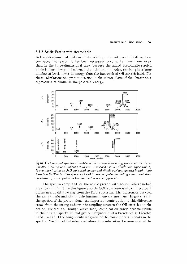
Results and Discussion 57
3.3.2 Acidic Proton with Acetonitrile
In the vibrational calculations of the acidic proton with acetonitrile we have
computed 120 levels. It has been necessary to compute many more levels
than in the three-dimensional case, because the added acetonitrile stretch
mode is much lower in frequency than the proton modes, resulting in a large
number of levels lower in energy than the �rst excited OH stretch level. For
these calculations the proton position in the mirror plane of the cluster does
represent a minimum in the potential energy.
a)
05
10152025
0 500 1000 1500 2000 2500 3000 3500 4000
inte
nsi
ty
90777
1214
1670 253831663184
32563270
33603386
b)
05
10152025
0 500 1000 1500 2000 2500 3000 3500 4000
inte
nsi
ty
119 776
11571693
23842507
2596
26252650
27692787
c)
0
20
40
60
80
0 500 1000 1500 2000 2500 3000 3500 4000
inte
nsi
ty
wave number
122 441 1016
2864
acet
on
itri
le
o.o
.p. b
end
i.p. b
end
stre
tch
Figure 3. Computed spectra of zeolite acidic proton interacting with acetonitrile, at
T=298.15 K. Wave numbers are in cm�1 , intensity is in 105m2=mol. Spectrum a)
is computed using an SCF potential energy and dipole surface, spectra b and c) are
based on DFT data. The spectra a) and b) are computed including anharmonicities,
spectrum c) is computed in the double harmonic approach.
The spectra computed for the acidic proton with acetonitrile adsorbed
are shown in Fig. 3. In this �gure also the SCF spectrum is shown, because it
di�ers in a qualitative way from the DFT spectrum. The di�erences between
the anharmonic and the double harmonic spectra are much larger than in
the spectra of the proton alone. An important contribution to this di�erence
stems from the strong anharmonic coupling between the OH stretch and the
acetonitrile stretch, through which many combination bands become visible
in the infrared spectrum, and give the impression of a broadened OH stretch
band. In Tab. 4 the assignments are given for the most important peaks in the
spectra. We did not list integrated absorption intensities, because most of the

58 Chapter 3: Three and Four-Coordinate Cluster Models
visual peaks are a superposition of transitions of which the low and high level
di�er the same number in the excitation level of the acetonitrile stretch; there
are more than a hundred transitions that give a substantial contribution to
the visible bands. Among the transitions that give substantial contributions,
i.e., at least 1 to 10 km/mol, the acetonitrile stretch may be excited as high
as to the seventh level.
Table 4. Computed IR spectrum of the acidic proton with acetonitrile. The as-
signment column shows the quantum numbers of the basis function with the largest
coeÆcient for the involved states; the �rst quantum number refers to the OH stretch,
the second to the in-plane bending, the third to the out-of-plane bending, and the
fourth to the acetonitrile stretch. � is the absorption frequency. All wave numbers
not in brackets are printed in Fig. 3. The values in brackets represent transitions
of little or no absorption intensity.
SCF DFT DFT
Anharmonic Anharmonic Double Harmonic
�(cm�1) �(cm�1) assignment �(cm�1)
90 119 0000 ! 0001 122
(774) 776 0001 ! 0011 441
777 (783) 0000 ! 0010 441
1214 1157 0000 ! 0100 1016
1670 1693 0000 ! 0020 (883)
2538 2384 0000 ! 0200 (2031)
(2708) 2596 0000 ! 0202 (2275)
3166 2507 0001 ! 1000 (2742)
3184 (2395) 0002 ! 1001 (2742)
3256 2625 0000 ! 1000 2864
3270 2650 0001 ! 1001 2864
3360 2769 0000 ! 1001 (2986)
(3362) 2787 0001 ! 1002 (2986)
3386 (2811) 0002 ! 1003 (2986)
Again it is seen that the anharmonic calculations generate a lower OH
stretch frequency compared to the harmonic calculations. All bending fre-
quencies are higher in the anharmonic calculations, and this e�ect is particu-
larly strong for the out-of-plane bending, which almost doubles in frequency
compared to the harmonic calculations.
A very marked change occurring upon acetonitrile adsorption is the in-
crease in infrared absorption intensity. Note the di�erent scales used on the
intensity axes comparing Fig. 2 and 3. This is caused by enhanced polarisa-
tion of the OH bond. For the DFT dipole surface, the component of the dipole
in the direction of the OH bond is �0:48 ea0 for the zeolite cluster without

Results and Discussion 59
acetonitrile, and 2:15 ea0 for the zeolite cluster with acetonitrile. The gradient
of the dipole in the OH bond direction increases from 0:46 e to 1:52 e upon
acetonitrile adsorption. Because the dominant term in the infrared absorp-
tion intensity of a transition between two adjacent OH stretch levels contains
the square of this gradient, an increase of the intensity by roughly a factor
of ten is to be expected. This is seen most clearly comparing the harmonic
spectra in Fig. 2 and 3, because they have all intensity due to the OH stretch
concentrated at a single wave number, whereas in the anharmonic spectra it
is spread over a greater number of peaks.
The changes in the infrared spectrum brought about by acetonitrile ad-
sorption are considerably larger for the DFT calculation than for the SCF
calculation. This con�rms our expectation that the DFT potential energy
surface should yield a spectrum that is closer to experiment. In Tab. 5 the
frequency shifts of the OH stretch and bendings are given. The shift of the
OH stretch appears to be not very sensitive to anharmonicities. The upward
shifts of the bendings are much larger in the anharmonic calculations.
Table 5. Frequency shifts upon acetonitrile adsorption in cm�1 .
stretch in-plane bending out-of-plane bending
SCF anharmonic �523 + 88 +299
SCF harmonic �527 � 36 + 24
DFT anharmonic �760 +148 +359
DFT harmonic �745 + 64 � 31
In the following discussion transitions between vibrational states are de-
noted in the same way as in the previous section, with a fourth quantum
number added to describe excitations in the acetonitrile stretch mode. In the
four-dimensional calculations the overtones of the out-of-plane bending are
visible with enhanced intensity at 1670 cm�1 (SCF) and 1693 cm�1 (DFT).
In the calculation with the SCF potential, the main OH stretch (0000! 1000)
peak at 3256 cm�1 is anked by di�erence (0001 ! 1001) and combination
(0000 ! 1001) bands with the acetonitrile stretch mode, and separate from
the overtone of the in-plane bending at 2538 cm�1. In the four-dimensional
DFT calculation the main OH stretch peak at 2625 cm�1 is anked on the high
frequency side by combination bands with the acetonitrile stretch, whereas on
the low frequency side the overtone of the in-plane bending and this overtone
combined with a doubly excited acetonitrile stretch yield the most impor-
tant peaks (0000 ! 0200 and 0000 ! 0202). The latter peaks have a rela-
tively large intensity due to the fact that the strongly absorbing OH stretch
mode mixes with the in-plane bending overtone vibrational states. This hap-
pens because the frequencies of the OH stretch and the in-plane bending
overtone are moving into each other's direction upon acetonitrile adsorption:

60 Chapter 3: Three and Four-Coordinate Cluster Models
the in-plane bending mode moves to a higher frequency because acetonitrile
pulls the proton in the direction of the mirror plane of the cluster, and the
OH stretch frequency decreases because the interaction with acetonitrile weak-
ens the OH bond. The SCF potential energy surface reproduces this e�ect
less well, so that there is not much mixing of the OH stretch mode with the
in-plane bending overtone, causing the intensity of the 0000! 0200 transition
at 2538 cm�1 (Fig. 3) to have a much smaller value than the corresponding
peak in the DFT spectrum. The interaction of the OH stretch and the over-
tone of the in-plane bending in the DFT calculation can also be seen from
the coeÆcients of the basis functions in the vibrational wave functions that
represent the excited states of the peaks at 2384 cm�1, 2596 cm�1, 2625 cm�1,
and 2650 cm�1. These coeÆcients are listed in Tab. 6. All the states listed
appear to be mixtures of OH stretch and in-plane bending overtone modes.
Table 6. Largest coeÆcients of basis functions of 4 vibrational states. Of four fre-
quencies in Tab. 4 the largest coeÆcients of basis functions of the higher level of the
transition are given. The basis functions are labelled by the order of Hermite func-
tion of OH stretch, in-plane bending, out-of-plane bending, and acetonitrile stretch
coordinate respectively. The coeÆcients of the basis functions are normalised, as
well as the basis functions themselves.
2384 cm�1 2586 cm�1 2625 cm�1 2650 cm�1
function coe�. function coe�. function coe�. function coe�.
0200 +0:880 0202 +0:637 1000 �0:728 1001 +0:669
1000 �0:285 0203 +0:367 0201 +0:266 1000 +0:344
0220 �0:230 1000 �0:235 0200 �0:242 1002 �0:2720400 �0:177 1001 +0:234 1001 +0:219 0201 +0:223
0201 +0:091 1002 �0:227 0202 �0:199 0202 �0:222
Pelmenschikov et al.[6] suggested that the bands observed around 2800
and 2400 cm�1 in experiment were due to a Fermi resonance between a very
strongly broadened OH stretch band (�1=2 � 800 cm�1) and a rather sharper
in-plane OH bending overtone. That would imply that the maxima correspond
to combinations of these modes. In our present results we do �nd peaks at
2625 cm�1 and 2384 cm�1 that are combinations of OH stretch and in-plane
bending overtone. However, the di�erence in frequency is smaller than in
the experiment, and the di�erence in intensity is much larger than in experi-
ment; the experimental bands are approximately equally intense. Apparently
the interaction between the OH stretch and the in-plane bending mode in
our model is less strong than experimentally. In our model the OH stretch
frequency should still get somewhat lower, or the in-plane bending overtone
frequency should get somewhat higher, or both. In other words, the proton in
our cluster model calculation does not interact strongly enough with acetoni-
trile; it is not acidic enough. In the following we will �rst discuss the e�ect of

Results and Discussion 61
the acetonitrile stretch mode and the in-plane bending mode on the spectrum,
and then try to improve on our model, in order to describe and explain the
experimental spectrum.
a)
0
20
40
60
0 500 1000 1500 2000 2500 3000
inte
nsi
ty
784 1158 1700 2383
2655
2790
b)
0
10
20
30
0 500 1000 1500 2000 2500 3000
inte
nsi
ty
7761157
1693 238425072596
26252650
27692787
c)
0
10
20
30
0 500 1000 1500 2000 2500 3000
inte
nsi
ty
wave number
763 16332469
2498
25982615
27372754
Figure 4. The in uence of the OH in-plane bending and the acetonitrile stretch on
the spectrum of the acidic proton with acetonitrile. All spectra are computed from
DFT potential energy and dipole surfaces, at T=298.15 K, including anharmonic-
ities. Wave numbers are in cm�1 , intensity is in 105m2=mol. In spectrum a) the
acetonitrile stretch mode is �xed, in spectrum c) the in-plane bending mode is �xed.
For comparison spectrum b) is plotted, without any modes �xed.
To check the in uence of the acetonitrile stretch and the in-plane bend-
ing mode of the acidic H, we did calculations with these modes �xed. The
results are shown in Fig. 4. If we compare the spectrum computed with
the acetonitrile stretch �xed with the spectrum with no modes �xed, we see
that coupling of the OH stretch mode with the acetonitrile stretch mode is
a good candidate as a cause of the broadening of the band. The intensity
of the OH stretch is `smeared' out over a wider frequency range. The spec-
trum where the in-plane bending is �xed allows for study of the interaction
of the acetonitrile stretch only, without interference of the in-plane bend-
ing overtone. There we see that the main OH stretch adsorption band is
anked by di�erence and combination bands of the OH stretch mode with
the acetonitrile stretch mode. Only transitions that di�er one excitation level
in the acetonitrile stretch have a substantial contribution. From the spec-
trum a guess of the half width of the broadened OH stretch band could be

62 Chapter 3: Three and Four-Coordinate Cluster Models
made of 2754 cm�1 � 2469 cm�1 = 285 cm�1. In earlier explanations of the
phenomenon, [3, 5, 6] it was assumed that the OH stretch band was broad-
ened to a width that comprises both mixed bands, through a coupling of the
OH stretch mode with the acetonitrile stretch. This implies for the current
system that, in order to reach the width of 800 cm�1 suggested in [6], the
OH stretch mode should yield visible combination bands with the acetoni-
trile stretch up to the third or fourth excited level: from 0003 ! 1000 or
0004! 1000, to 0000! 1003 or 0000! 1004. As an alternative explanation
for the experimental spectrum we suggest that there is a resonance of the in-
plane bending overtone with an OH stretch band, resulting in two vibrational
states that both are mixtures of the two modes. A broadening of the order of
300 cm�1 is seen in both mixed mode bands, at 2400 cm�1 and 2800 cm�1.
In an attempt to render our model somewhat more `acidic', we have mod-
i�ed the DFT potential. We have stretched it in the OH stretch coordinate,
making the potential atter in order to lower the OH stretch frequency, and at
the same time compressed it by the same scale factor in the in-plane bending
coordinate, making it steeper in order to increase the in-plane bending fre-
quency. In Fig. 5 the spectrum that is obtained by application of a scale factor
of 1.05 is shown. The unscaled DFT dipole surface has been used to compute
it. This spectrum very much resembles the experimental spectra, showing two
main broadened bands that are due to combinations of the in-plane bending
overtone and the OH stretch mode. The most signi�cant di�erence with the
experimental spectra is the distance between the two peaks, which is smaller
in the computation.
0
10
20
30
0 500 1000 1500 2000 2500 3000
inte
nsi
ty
wave number
Figure 5. Computed spectrum of zeolite acidic OH with acetonitrile, at T=298.15 K.
Wave numbers are in cm�1 , intensity is in 105m2=mol. The DFT potential energy
surface has been scaled (see text).
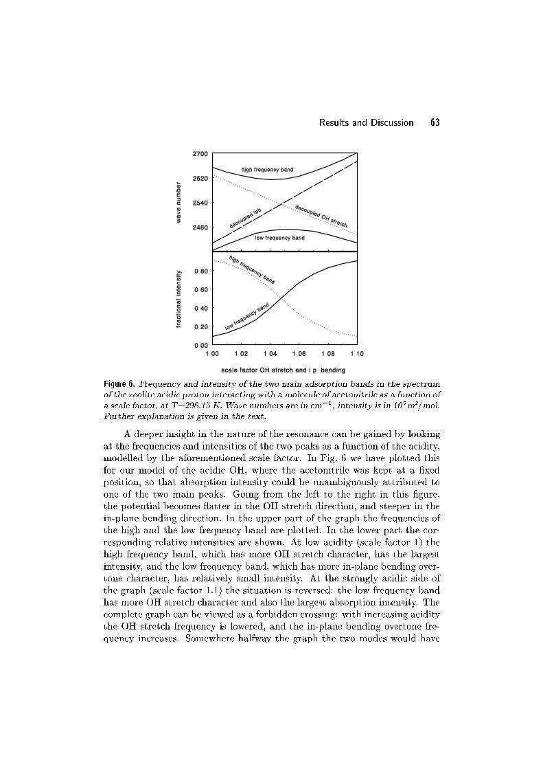
Results and Discussion 63
Figure 6. Frequency and intensity of the two main adsorption bands in the spectrum
of the zeolite acidic proton interacting with a molecule of acetonitrile as a function of
a scale factor, at T=298.15 K. Wave numbers are in cm�1 , intensity is in 105m2=mol.
Further explanation is given in the text.
A deeper insight in the nature of the resonance can be gained by looking
at the frequencies and intensities of the two peaks as a function of the acidity,
modelled by the aforementioned scale factor. In Fig. 6 we have plotted this
for our model of the acidic OH, where the acetonitrile was kept at a �xed
position, so that absorption intensity could be unambiguously attributed to
one of the two main peaks. Going from the left to the right in this �gure,
the potential becomes atter in the OH stretch direction, and steeper in the
in-plane bending direction. In the upper part of the graph the frequencies of
the high and the low frequency band are plotted. In the lower part the cor-
responding relative intensities are shown. At low acidity (scale factor 1) the
high frequency band, which has more OH stretch character, has the largest
intensity, and the low frequency band, which has more in-plane bending over-
tone character, has relatively small intensity. At the strongly acidic side of
the graph (scale factor 1.1) the situation is reversed: the low frequency band
has more OH stretch character and also the largest absorption intensity. The
complete graph can be viewed as a forbidden crossing: with increasing acidity
the OH stretch frequency is lowered, and the in-plane bending overtone fre-
quency increases. Somewhere halfway the graph the two modes would have

64 Chapter 3: Three and Four-Coordinate Cluster Models
the same frequency, if they did not couple. Since they do couple, the levels are
split. The frequency of decoupled OH stretch and in-plane bending overtone
modes can be computed assuming that all of the infrared absorption intensity
is due to the OH stretch mode. This is a fairly accurate assumption for the
given system. The derivation of the formulae used to compute the decoupled
frequencies plotted in Fig. 6 is given in the Appendix.
a)
0
20
40
60
80
500 1000 1500 2000 2500 3000
inte
nsi
ty
b)
0
20
40
60
80
500 1000 1500 2000 2500 3000
inte
nsi
ty
c)
0
20
40
60
80
500 1000 1500 2000 2500 3000
inte
nsi
ty
wave number
Figure 7. Computed spectra of zeolite acidic proton with acetonitrile, with acetoni-
trile �xed at equilibrium position, at T=298.15 K. Wave numbers are in cm�1 ,
intensity is in 105m2=mol. The spectra are based on the DFT potential energy and
dipole surfaces, they di�er in scale factor for the OH stretch and in-plane bending
modes. Spectrum a) has a scale factor of 1.00, spectrum b) has a scale factor of
1.05, and spectrum c) has a scale factor of 1.10. The scaled potential energy sur-
faces model zeolite OH groups that are more acidic going from a) to c). The spectra
correspond to the left, middle and right of Fig. 6.
Fig. 6 shows that in a certain range of di�erent scale factors the frequen-
cies of the two main peaks due to hydrogen bonding do not vary strongly,
whereas the intensity is transferred from the high frequency band to the low
frequency band. This transfer of intensity is illustrated by Fig. 7, which shows
the spectra corresponding to the left, middle, and right of Fig. 6. The position
of the dip between the two bands, de�ned as the average of the frequencies
of the two bands, stays approximately the same in the whole range of scale
factors tested, and corresponds to the place where the decoupled OH stretch
and in-plane bending overtone cross each other.

Results and Discussion 65
In Fig. 8 the computed spectrum (scale factor 1.05) of the acidic proton
with acetonitrile is shown both at room temperature (298.15K) and liquid ni-
trogen temperature (77K). The most marked di�erence is the fact that at low
temperature the absorption intensity is concentrated in fewer peaks. Cooling
down to even lower temperatures (liquid helium, 4.2K) doesn't make much
further di�erence. For the modes we studied it appears as though measure-
ments at low temperature might give a better resolution, but the experimental
spectrum could still be blurred by coupling of lattice modes, and inhomoge-
neous line broadening. In the computed spectra also some broadening of the
two-band system is observed when going to a higher temperature.
0
20
40
1600 1800 2000 2200 2400 2600 2800 3000
inte
nsi
ty
T = 77K
0
20
40
1600 1800 2000 2200 2400 2600 2800 3000
inte
nsi
ty
wave number
T = 298K
Figure 8. Computed spectra of zeolite acidic proton interacting with acetonitrile, at
T=77 K and at T=298.15 K. Wave numbers are in cm�1 , intensity in 105m2=mol.
The spectra are computed using DFT (scale factor 1.05) potential energy and dipole
surfaces.
An interesting, though small, temperature e�ect is that the overall inten-
sity of the spectrum decreases by 3.43% going from 77K to 298.15K (com-
puted with the unscaled potential energy). This is probably due to the larger
distance between the OH group and the acetonitrile molecule at higher tem-
peratures, that results in a smaller interaction. Taking into account the Boltz-
mann distributions over the di�erent vibrational levels, we have computed the
average distance between acetonitrile and the O atom of the OH group to grow
by 0.027�A going from 77K to 289.15K (again for the unscaled potential).

66 Chapter 3: Three and Four-Coordinate Cluster Models
3.4 Conclusions
The experimentally observed splitting of OH stretch infrared absorption bands
upon adsorption of a basic molecule can be explained by the interaction of
the OH in-plane bending overtone with the OH stretch mode. The two main
absorption bands seen in experiment are both due to di�erently mixed in-plane
bending and OH stretch modes.
More acidic OH groups have a relatively more intense low frequency OH
stretch absorption band, compared to the high frequency band, if a basic
molecule is absorbed. The dip between the two main absorption bands is
approximately at the position where the decoupled OH stretch and in-plane
bending mode would cross each other with increasing acidity.
The used (HO)3Al(OH)Si(OH)3 zeolite cluster seems to be not \acidic"
enough if, at DFT level, only the H atom is allowed to move. This may be
due to the limited number of degrees of freedom considered, to shortcomings
of the cluster molecule as a model of the zeolite. From a test calculation of
the silanol OH stretch frequency it appears that the applied DFT method is
valid for the computation of infrared spectra.
Acknowledgement
E.L. Meijer gratefully acknowledges �nancial support by Shell laboratories in
Amsterdam (KSLA) for the beginning of his graduate research.
Appendix: Derivation of Decoupled Mode Frequencies
The OH stretch and overtone in-plane bending modes are strongly coupled
if there is hydrogen bonding to a molecule of acetonitrile. In this paper we
estimated the frequencies of the decoupled modes in a way that can be applied
to experimental data as well. The formulae used to compute the frequencies
are deduced as follows.
Let j�0i be the vibrational ground state, and j�1i and j�2i the mixed
states of OH stretch and the overtone of the in-plane bending that occur as
eigenstates of the Hamiltonian. Let j 1i be the decoupled excited OH stretch
state, and j 2i the decoupled doubly excited in-plane bending state. The
coupled states can be written as linear combinations of the decoupled states:
j�ii =Xj
cijj ji; (5)
where fcijg are the coeÆcients of an orthogonal 2 � 2 matrix. In good ap-
proximation it can be assumed that the absorption intensity of the transitions
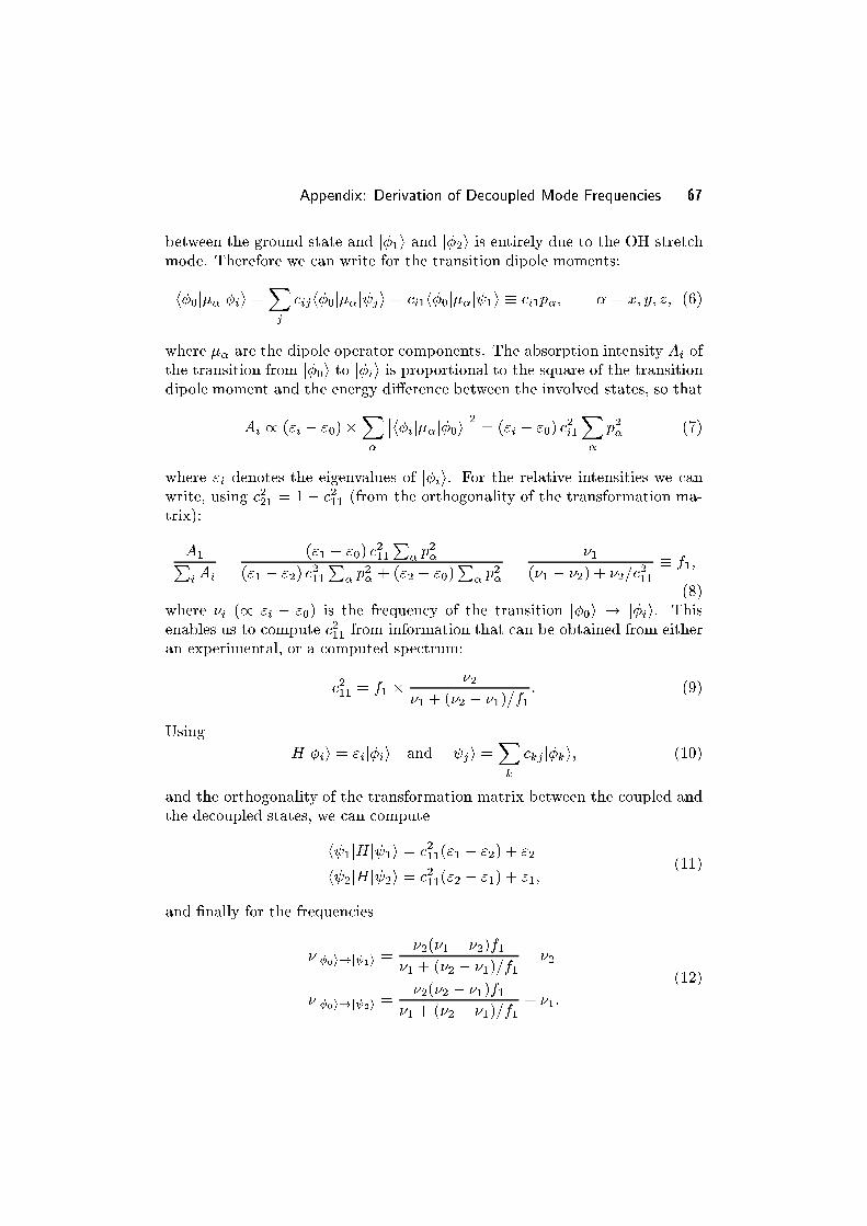
Appendix: Derivation of Decoupled Mode Frequencies 67
between the ground state and j�1i and j�2i is entirely due to the OH stretch
mode. Therefore we can write for the transition dipole moments:
h�0j��j�ii =Xj
cijh�0j��j ji = ci1h�0j��j 1i � ci1p�; � = x; y; z; (6)
where �� are the dipole operator components. The absorption intensity Ai of
the transition from j�0i to j�ii is proportional to the square of the transitiondipole moment and the energy di�erence between the involved states, so that
Ai / ("i � "0)�X�
��h�ij��j�0i��2 = ("i � "0) c2i1X�
p2� (7)
where "i denotes the eigenvalues of j�ii. For the relative intensities we can
write, using c221 = 1� c211 (from the orthogonality of the transformation ma-
trix):
A1PiAi
=("1 � "0) c211
P� p
2�
("1 � "2) c211P
� p2� + ("2 � "0)
P� p
2�
=�1
(�1 � �2) + �2=c211
� f1;
(8)
where �i (/ "i � "0) is the frequency of the transition j�0i ! j�ii. This
enables us to compute c211 from information that can be obtained from either
an experimental, or a computed spectrum:
c211 = f1 �
�2
�1 + (�2 � �1)=f1: (9)
Using
Hj�ii = "ij�ii and j ji =Xk
ckjj�ki; (10)
and the orthogonality of the transformation matrix between the coupled and
the decoupled states, we can compute
h 1jHj 1i = c211("1 � "2) + "2
h 2jHj 2i = c211("2 � "1) + "1;
(11)
and �nally for the frequencies
�j�0i!j 1i =�2(�1 � �2)f1
�1 + (�2 � �1)=f1+ �2
�j�0i!j 2i =�2(�2 � �1)f1
�1 + (�2 � �1)=f1+ �1:
(12)

68 Chapter 3: Three and Four-Coordinate Cluster Models
References
[1] L. Kubelkov�a, J. Nov�akov�a, and K. Nedomov�a; J. Catal., \Reactivity
of Surface Species on Zeolites in Methanol Conversion", 124, 441{450
(1990).
[2] G. Mirth, J. A. Lercher, M. W. Anderson, and J. Klinowski; J. Chem.
Soc. Faraday Trans., \Adsorption Complexes of Methanol on Zeolite
ZSM-5", 86, 3039{3044 (1990).
[3] M. F. Claydon, and N. Sheppard; Chemical Communications, \The Na-
ture of \A,B,C"-type Infrared Spectra of Strongly Hydrogen-bonded Sys-
tems; Pseudo-maxima in Vibrational Spectra", 1431{1433 (1969).
[4] S. E. Odinokov, and A. V. Iogansen; Spectrochim Acta, \Torsional
(OH) vibrations, Fermi resonance [ (OH) , �(OH)] and isotopic ef-
fects in i.r. spectra of H-complexes of carboxylic acids with strong bases",
28A, 2343{2350 (1972).
[5] N. Sheppard; Hydrogen bonding; ed. D. Had�zi;, Pergamon, San Francisco
& London, 1960
[6] A. G. Pelmenschikov, R. A. van Santen, J. J�anchen, and E. L. Meijer;
J. Phys. Chem., \CD3CN as a Probe of Lewis and Br�nsted Acidity of
Zeolites", 97, 11071{11074 (1993).
[7] A. D. Becke; J. Chem. Phys., \Density-functional thermochemistry. III.
The role of exact exchange.", 98, 5648{5652 (1993).
[8] A. D. Becke; Phys. Rev. A, \Density-functional exchange-energy ap-
proximation with correct asymptotic behavior", 38, 3098{3100 (1988).
[9] C. Lee, W. Wang, and R. G. Parr; Phys. Rev. B, \Development of the
Colle-Salvetti correlation-energy formula into a functional of the electron
density", 37, 785{789 (1988).
[10] S. H. Vosko, L. Wilk, and M. Nusair; Can. J. Phys., \Accurate spin-
dependent electron liquid correlation energies for local spin density cal-
culations: a critical analysis", 58, 1200{1211 (1980).
[11] A. A. Rashin, L. Young, I. A. Topol, and S. K Burt; Chem. Phys.
Letters, \Molecular dipole moments calculated with density functional
theory", 230, 182{188 (1994).
[12] W. J. Hehre, R. F. Stewart, and J. A. Pople; J. Chem. Phys., \Self-
Consistent Molecular-Orbital Methods. I. Use of Gaussian Expansions of
Slater-Type Atomic Orbitals", 51, 2657{2664 (1969).
[13] M. S. Gordon, J. S. Binkley, J. A. Pople, W. J. Pietro, and W. J.
Hehre; J. Am. Chem. Soc., \Self-Consistent Molecular-Orbital Methods.
22. Small Split-valence Basis-Sets for Second-Row Elements", 104, 2797{
2803 (1982).
References 69
[14] W. J. Hehre, R. Ditch�eld, and J. A. Pople; J. Chem. Phys., \Self-
ConsistentMolecular-OrbitalMethods. XII. Further Extensions of Gauss-
ian-Type Basis Sets for Use in Molecular-Orbital Studies of Organic
Molecules", 56, 2257{2261 (1971).
[15] M. M. Francl, W. J. Pietro, W. J. Hehre, J. S. Binkley, M. S. Gor-
don, D. J. Defrees, and J. A. Pople; J. Chem. Phys., \Self-Consistent
Molecular-Orbital Methods. XXIII. A Polarization-Type Basis Set for
Second Row Elements", 77, 3654{3665 (1986).
[16] P. C. Hariharan, and J. A. Pople; Theor. Chim. Acta, \The In uence of
Polarization Functions on Molecular-Orbital Hydrogenation Energies.",
28, 213{222 (1973).
[17] R. Krishnan, J. S. Binkley, R. Seeger, and J. A. Pople; J. Chem.
Phys., \Self-Consistent Molecular-Orbital Methods. XX. A basis set for
correlated wave functions", 72, 650{654 (1973).
[18] T. Clark, J. Chandrasekhar, G. W. Spitznagel, P. v. R. Schleyer,
J. Comp. Chem., \EÆcient Di�use Function-Augmented Basis Sets for
First-Row Elements, Li{F", 4, 294{301 (1982).
[19] D. J. Defrees, and A. D McLean; J. Comp. Chem., \Ab Initio Determi-
nation of the Proton AÆnities of Small Neutral and Anionic Molecules",
7, 321{333 (1986).
[20] J. F. Haw, M. B. Hall, A. E. Alvaro-Swaisgood, E. J. Munson, Z. Lin,
L. W. Beck, and T. Howard; J. Am. Chem. Soc., \Integrated NMR and
Ab Initio Study of Acetonitrile in Zeolites: A Reactive Complex Model
of Zeolite Acidity", 116, 7308{7318 (1994).
[21] M. J. Frisch, G. W. Trucks, H. B. Schlegel, P. M. W. Gill, B. G.
Johnson, M. W. Wong, J. B. Foresman, M. A. Robb, M. Head-
Gordon, E. S. Replogle, R. Gomperts, J. L. Andres, K. Raghavachari,
J. S. Binkley, C. Gonzalez, R. L. Martin, D. J. Fox, D. J. Defrees, J.
Baker, J. J. P. Stewart, and J. A. Pople; Gaussian 92/DFT, Revision
F.2; Gaussian, Inc., Pittsburgh PA, 1993
[22] W. H. Press, B. P. Flannery, S. A. Teukolsky, and W. T. Vetterling;
Numerical Recipes in C, The Art of Scienti�c Computing; Cambridge
University Press, Cambridge, 1988, Chap. 2.9
[23] E. B. Wilson, Jr., J. C. Decius, and P. C. Cross; Molecular Vibrations;
Mc-Graw-Hill, New York, Toronto, London, 1955
[24] A. Messiah; Quantum Mechanics; John Wiley & Sons, New York, 1974,
Chap. XII
[25] C. Mijoule, M. Allavena, J. M. Leclerq, and Y. Bouteiller; Chemical
Physics, \Theoretical Vibrational Study of the Symmetric �OH and �O���OStretching Modes of the Formic Acid Dimer in the Gas Phase", 109, 207{
213 (1986).
70 Chapter 3: Three and Four-Coordinate Cluster Models
[26] L. Pauling, and E. B. Wilson; Introduction to Quantum Mechanics
(McGraw-Hill, 1935, Chap. XI)
[27] C. J. Lanczos; J. Res. Natl. Bur. Stand., 45, 255 (1950).
[28] B. N. Parlett; The Symmetric Eigenvalue Problem; Prentice-Hall, Engle-
wood Cli�s, NJ, 1980
[29] D. E. Stewart, and Z. Leyk; Meschach: Matrix Computations in C; Cen-
tre for Mathematics and its Applications, Australian National University,
Canberra, 1994
[30] H. V. Brand, L. A. Curtiss, and L. E. Iton; J. Phys. Chem., \Computa-
tional Studies of Acid Sites in ZSM-5: Dependence on Cluster Size", 96,
7725{7732 (1992).
[31] A. G. Pelmenschikov, G. Morosi, and A. Gamba; J. Phys. Chem.,
\Quantum Chemical Molecular Models of Oxides. 1. Reproduction of
Vibrational Frequencies of Surface OH Groups", 95, 10037{10041 (1991).

4Six and Seven-Coordinate Cluster Models
Abstract
The e�ect of acetonitrile adsorption on the infrared spectrum of an acidic
hydroxyl group of a zeolite was studied using quantum-chemical calculations.
The hydroxyl and its surroundings in the zeolite were modeled by a cluster
molecule. Potential energy and dipole surfaces of the model were computed
with Density Functional Theory applying the Becke3LYP functional. A poten-
tial energy surface has been constructed as a function of the stretch, in-plane
bending, and out-of-plane bending coordinates of both the hydrogen and the
oxygen atom of the hydroxyl group, as well as the center-of-mass stretch coor-
dinate of acetonitrile. Taking into full account anharmonicities, we computed
the vibrational wave functions and infrared absorption intensities using a vari-
ational approach. To facilitate their interpretation, the computed spectra were
decomposed with respect to the di�erent vibrational coordinates. It was found
that the use of centre of mass conserving coordinates for the hydroxyl group is
insuÆcient to obtain accurate hydroxyl stretch frequencies, and that oxygen
coordinates need to be included in the calculation. The inclusion of oxygen
coordinates furthermore improves the computed Fermi resonance splitting. A
new explanation for the width of the A,B spectra is proposed.
Reproduced in part from E.L. Meijer, R.A. van Santen, and A.P.J. Jansen:
\Infrared Spectrum of an Acidic Zeolite OH with Adsorbed Acetonitrile",
J. Phys. Chem. A 103 2553{2560 (1999). Copyright 1999 American Chemical
Society.

72 Chapter 4: Six and Seven-Coordinate Cluster Models
4.1 Introduction
Zeolites are crystalline materials consisting mainly of SiO4 tetrahedra that
are linked through sharing of oxygen atoms. They appear in many di�erent
crystal structures that exhibit channels and cages of molecular dimensions (4{
12�A). In most zeolites a fraction of the silicon atoms is replaced by aluminium
atoms. The negative charge this introduces into the lattice can be balanced by
a proton attached to the oxygen atoms that bridges a silicon and an aluminium
atom, thus forming a bridged hydroxyl with strong Br�nsted acidity. The
combination of these acidic sites with the well-de�ned micro-pores makes them
suitable catalysts for a range of reactions.
In the infrared spectrum of a zeolite, the bridged hydroxyl stretch mode is
observed in the range 3605{3615 cm�1. If a weakly basic molecule is adsorbed
on the hydroxyl, the stretch frequency shifts down to lower values. The shift
that occurs with a certain base molecule has been proposed as a measure for
the acidity of the bridging hydroxyl ([1], and references therein). For this
application weak bases like CO and N2 that only cause small shifts are most
suitable.[2, 3]
Acetonitrile is among the strongest basic molecules that will disturb a
bridging hydroxyl, but not subtract a proton from it. The infrared spectrum
resulting is more complicated than that of weaker bases. It displays a large
downward shift (800{1200 cm�1) of the hydroxyl stretch band, as well as a
marked splitting and broadening of the band. The resulting two main broad
bands at 2400 and 2800 cm�1 are usually referred to as the A,B-dyad. Some-
times a third band, denoted `C' is seen at even lower frequencies. This band
is usually less clear. Conclusive experimental evidence exists that these bands
are due to one single type of complex, where acetonitrile is hydrogen bonded
to the bridging hydroxyl.[1, 4, 5]
The characteristic splitting of the shifted hydroxyl stretch band into
the A,B-dyad is caused by a Fermi resonance between a broadened hydroxyl
stretch band (�), and the overtone of the in-plane (Æ) hydroxyl bending, where
the `plane' refers to the plane formed by the Si{O{Al group on which the extra
proton sits.
Empirical models have been applied to describe the spectra[6{8]. In ear-
lier work we tried to compute the infrared spectrum from �rst principles,[9]
taking into account only a minimal set of vibrational coordinates: the coor-
dinates of the hydrogen atom of the hydroxyl group, and the intermolecular
stretch of the acetonitrile molecule as a whole with respect to the hydroxyl.
Using this simple model we could show that among the vibrational wave func-
tions computed on the basis of a density functional potential energy surface
Fermi resonances did occur. However, the computed width of the A,B bands,

Calculation of Potential Energy and Dipole Surfaces 73
the size of the A,B splitting, and the stretch frequency of the free bridged hy-
droxyl left room for improvement. In the current paper we present the results
of an extension of the former model to include the dynamics of the oxygen
atom. Based on this model, we propose an interpretation of the nature of the
A,B-spectra that di�ers from the empirical models mentioned.
4.2 Calculation of Potential Energy and Dipole Surfaces
The acidic OH group of the zeolite is represented by a small, neutral, clus-
ter molecule, terminated by hydroxyl groups. This model is shown in Fig. 1,
along with the coordinates we used in the vibrational calculations. All coor-
dinates are linear combinations of atomic displacements. Electronic structure
calculations have been used to compute potential energy and dipole surfaces
as a function of a limited number of degrees of freedom.
NC
C
H
Al
H
Si
O
out-
in-plane bending
stretch
in-plane bending
stretch
of-
bendingplane
out-
planebending
of-
O HOH
H H
OH OH
OHO H
acetonitrile
stretchcenter of mass
Figure 1. The zeolite cluster model with adsorbed acetonitrile. The vibrational
coordinates used in the calculations are shown as arrows.
In a previous paper,[9] where we presented calculations of anharmonic
coupling e�ects, we only considered the stretch, in-plane, and out-of-plane
coordinates of the hydrogen atom, and the stretch of the H� � �N hydrogen

74 Chapter 4: Six and Seven-Coordinate Cluster Models
bridge, with acetonitrile as a rigid particle. Here we also include the move-
ment of the oxygen atom of the OH group for the acidic OH group and the
acidic OH group with adsorbed acetonitrile. We extended the potential energy
and dipole surfaces used in the previous work to obtain 6- and 7-dimensional
versions
4.2.1 Electronic Structure Calculations
The potential energy surfaces used are based on density functional theory
electronic structure calculations using Becke's three-parameter functional with
the non-local correlation provided by the Lee, Yang, and Parr expression [10{
13]. We have demonstrated earlier[9] that this method gives results that
are signi�cantly better than those obtained with Hartree-Fock. Therefore
we have not extended the Hartree-Fock potentials from the previous work.
The electronic structure calculations have been carried out with the Gaussian
92/DFT program package [14]. A mixed basis set has been used with STO-
3G [15] on the H atoms of the terminal OH groups, 6-311+G* [16{18] on the
central O atom of the zeolite cluster and the N atom of acetonitrile, and 6-
31G** [19{22] for the other atoms. This basis set describes the atoms that are
important in the interaction between the acidic hydroxyl and the acetonitrile
molecule accurately.[9] The minimal basis set on the terminal hydrogen atoms
of the cluster was used to reduce computational costs.
As a starting point for the potential energy surfaces, the zeolite cluster
as shown in Fig. 1 was optimized with and without adsorbed acetonitrile.
The optimization was restricted in two ways. Firstly, during the optimization
the plane through the central Si{OH{Al group was kept as a mirror plane,
in order to reduce the number of points that had to be computed for the
potential energy surface. Secondly, to prevent internal hydrogen bridging, the
(Si{O{H) and (Al{O{H) angles of the terminating OH groups were �xed at
tetrahedral angles, and, going from the central O atom to a terminal OH,
O{Si{O{H and O{Al{O{H atoms were required to stay in one plane.

Calculation of Potential Energy and Dipole Surfaces 75
4.2.2 Three and Four-Dimensional Potential Energy Surfaces
The three-dimensional potential energy surface is the potential energy of the
zeolite cluster as a function of the acidic hydrogen coordinates. It is based
on electronic structure calculations performed for a grid of acidic hydrogen
positions. The grid was constructed as follows: At �ve di�erent OH distances,
0.8, 0.9, 1.0, 1.1, and 1.4 times the equilibrium distance, the hydrogen atom
was bent toward the Al atom by an angle � of 0Æ, 7.5Æ, 20Æ, and 60Æ and
subsequently rotated around the axis de�ned by the equilibrium acidic OH
bond by an angle � of 0Æ, 45Æ, 90Æ, 135Æ, and 180Æ. The energies and dipoles
of geometries corresponding to � = 225Æ, 270Æ, and 315Æ were inferred from
the 135Æ, 90Æ, and 45Æ points taking into account the symmetry plane of the
cluster.
The four-dimensional potential describes the energy of the zeolite cluster
with a molecule of acetonitrile adsorbed as a function of the acidic hydrogen
coordinates and the acetonitrile center of mass stretch coordinate. All internal
acetonitrile coordinates were kept �xed. A grid of hydrogen positions has
been constructed in the same fashion as for the bare zeolite cluster, using the
equilibrium OH distance in the acidic hydroxyl with acetonitrile adsorbed.
For each of the points of this grid the electronic energy was computed for �ve
di�erent distances between acetonitrile and the oxygen atom of the zeolite
acidic OH group: the equilibrium distance r0, r0 � 0:15�A, and r0 � 0:5�A.
The potential energy points were �tted with fourth order polynomials.
For the �t each point i was attributed a �t weight wi according to the following
expression:
wi �e�f�viPNj e�f�vj
; (1)
Here vi is the electronic energy of point i, N the total number of points, and
f a positive factor that determines the relative weight of the points. This
expression attributes larger �t weights to data points with lower potential
energy. Physically, data points with low energy are relatively more signi�cant
for the correct description of the lower lying vibrational levels, which we want
to describe. The f parameter was given a value of 125Eh�1, so as to produce
a root mean square error smaller than 1 � 10�3Eh. The computed energies
for potentials were in an interval of approximately 0.2Eh.
All �ts in this paper were performed with singular value decomposition,
[23] in order to remove near-degeneracies. For the three and four-dimensional
�ts we had to set one of the singular values to zero. This means that one
degree of freedom of the polynomial was �xed through minimization of the
squares of the coeÆcients.
Both the three and four-dimensional potential had negative fourth order
coeÆcients for the hydrogen stretch coordinate. If basis functions were allowed

76 Chapter 4: Six and Seven-Coordinate Cluster Models
to extend into the area where the �tted potential approached negative in�nity,
unphysical vibrational wave functions would be computed. We have shown
earlier [9] that this problem does not occur in our three and four-dimensional
calculations, since the wave functions stay con�ned to an area where the �tted
potential interpolates between the computed data points.
4.2.3 Six-Dimensional Potential Energy Surface
The six-dimensional potential describes the potential energy of the zeolite
cluster, as a function of the position of the oxygen and hydrogen atoms of the
acidic OH group. In its construction the coeÆcients of the three-dimensional
potential for hydrogen displacement have been retained. The second order
coeÆcients for the oxygen coordinates and the bilinear coupling coeÆcients
for the oxygen coordinates among themselves, and with the hydrogen coordi-
nates, have been derived from the force constants computed in a Gaussian92
normal mode calculation. The potential thus constructed did not display the
desired asymptotic behaviour for large displacements of the atoms from their
origins. In certain directions, already at relatively small distances from the
equilibrium, the potential showed large negative values, giving rise to the
computation of unphysical vibrational states.
In order to improve the potential, extra data points of the potential energy
surface have been computed. The grid of extra points can be described in
terms of displacement vectors of oxygen and hydrogen. We de�ne x1 to be a
vector along the OH bond, x2 a vector in the direction perpendicular to the
OH bond in the Al{O{Si plane, and x3 a vector perpendicular to x1 and x2.
Initially a grid has been constructed from molecular geometries where
oxygen or both oxygen and hydrogen were displaced by �x1, �x2, �x3, or�(x1+x2+x3)=
p3. The lengths of the vectors xi are derived from the force
constants in the corresponding directions, in such a way that the displace-
ments correspond to eight times the r.m.s. displacement of a one-dimensional
harmonic vibration of the atom. This means that the vectors for hydrogen
displacement have di�erent lengths from those for oxygen. The �tted second
order coeÆcient of the potential energy with respect to the out-of-plane move-
ment of hydrogen is negative. This displacement has its length derived from
the force constant used for the basis function, as described in [9].
In some of the geometries generated in this grid the OH distance becomes
as small as 0.16 �A. Therefore we have applied a correction to the grid points
through expansion of the OH bond about its center of mass. The new OH
distance was computed from the old via a linear transformation that leaves the
maximum distance from the grid as it is, and expands the smallest distance to
0.5 times the equilibrium distance of the OH bond. If the maximum distance
in the original grid is rmax, the minimum distance rmin, and the equilibrium
Calculation of Potential Energy and Dipole Surfaces 77
OH distance req, then the new OH distances r0 are computed from the old r
using
r0 = r +
(rmax � r)(rmax � rmin)
� (req=2� rmin) (2)
The grid contains 210 points which were attributed �t weights as de-
scribed in Eq. 1, again with f = 125E�1h . In the singular value decomposition
procedure we had to set 47 singular values to zero. This means that 47 degrees
of freedom in the polynomial were left that were �xed by minimizing the sum
of the squares of the �tted coeÆcients. The potential such obtained proved
suitable for our calculations and no unphysical vibrational states were found
with the basis set we employed.
4.2.4 Seven-Dimensional Potential Energy Surface
The seven-dimensional potential energy surface describes the potential energy
of the zeolite cluster with adsorbed acetonitrile as a function of the coordi-
nates of the acidic OH group of the cluster, and the center of mass stretch
of acetonitrile. It has been constructed retaining the coeÆcients of the four-
dimensional potential, and quadratic terms for the oxygen movement and
bilinear coupling terms between oxygen and hydrogen coordinates have been
derived from a Gaussian normal mode calculation. Coupling terms between
the oxygen coordinates and the acetonitrile coordinate have been neglected,
because although they are small and have little physical importance, they can
give rise to problems with the asymptotic behaviour of the �tted polynomial
if no higher order coeÆcients are included as well.
As in the case of the six-dimensional potential, extra points of the poten-
tial energy surface had to be computed, and a grid similar to the one described
for the six-dimensional surface was employed. No extra points were used to
further probe the coupling of the oxygen coordinates and the acetonitrile co-
ordinate. The grid of the extra points for the seven-dimensional potential
was constructed with vectors xi (see above) of a length four times the one-
dimensional harmonic r.m.s. displacement of the atom. This is much nearer
to the origin than in the six-dimensional case, where the larger displacements
were necessary to get satisfactory asymptotic behaviour of the �tted poten-
tial. Because of the smaller displacements there was no need to adjust the
grid points afterwards to prevent too small inter-atomic distances.
Fit-weights were attributed to the extra points in the same manner as in
the six-dimensional case. In this case 41 singular values had to be set to zero.

78 Chapter 4: Six and Seven-Coordinate Cluster Models
4.2.5 Derivation of the dipole surfaces
For all the data points we used for the three and the four-dimensional potential
energy surfaces, also the x, y, and z-components of the dipole were computed.
Using the same �t weights as for the energy, the dipole surfaces were �tted
by fourth order polynomials.
To reduce computational cost we only used linear dipole surfaces for both
the six and the seven dimensional spectra. For the hydrogen and acetonitrile
coordinates the dipole coeÆcients up to �rst order computed from the three
and four-dimensional surfaces were used, for the oxygen coordinates the dipole
and dipole derivatives computed in a Gaussian92 normal mode calculation
were used.
From the three and four dimensional calculations it appears that the
computed spectra are hardly a�ected by the omission of higher order dipole
coeÆcients. As a test case we computed for the four dimensional spectrum
that the total absorbed intensity of the infrared spectrum at 298.15K, in
the range of 0 to 4000 cm�1, decreases by 0.35%comparing a linear dipole
surface to a fourth order dipole surface. For that same spectrum, the root
mean square di�erence in intensity on a per transition basis was about 3.2%.
Clearly, di�erences exist in both positive and negative directions and are of
minor importance.
4.3 Calculation of the Infrared Spectra
4.3.1 The Vibrational Hamiltonian
The Hamiltonian employed in the vibrational calculations is the following:
H =1
2
DXi=1
DXj=1
M�1ij pipj +
X�1;:::;�D
a�1;:::;�D
DYi=1
q�ii ; with 0 �
DXi=1
�i � N (3)
In this expressionD is the number of dimensions, qi are the spatial coordinates
with conjugated momenta pi, M�1 is the inverse mass matrix, and a�1;:::;�D
are the coeÆcients of the N th order polynomial representing the potential
energy [24]. For all the calculations in this paper, the polynomial order N has
been equal to four. The way the potential energy polynomial is truncated,
ensures that it's shape does not depend a on a particular choice of internal co-
ordinates. (It should be noted however, that the wave function space spanned
by the basis set is not independent from the choice of the coordinates.)
We choose to use a polynomial representation of the potential because it
has no bias toward a particular potential shape, and matrix elements can be
readily computed in the basis set we employed. To this e�ect the Hamilto-
nian was converted into a representation of normal products of creation and
annihilation operators [25].

Calculation of the Infrared Spectra 79
A disadvantage of the polynomial form of the potential is the unphysical
behaviour of the potential outside the area where data points were computed.
A polynomial potential goes to �1 where a physical potential levels o� to a
constant value. This is mainly a concern if the polynomial goes to �1. As
a result unphysical low energy vibrational states can occur in the calculation,
if the basis functions have non-negligible amplitude in the area where the
potential has unphysically low values. We have avoided such basis functions.
The o�-diagonal terms Mijpipj in the kinetic energy can have non-zero
values if the coordinates are not orthogonal. This was never the case in the
calculations described in this paper.
4.3.2 The Vibrational Basis Set
The wave functions are expanded in products of one-dimensional harmonic
eigenfunctions (Hermite functions).[24]
(q1; : : : ; qD) =X
�1;:::;�D
c�1;:::;�D
DYi=1
�(�i)(qi) (4)
In this expression is the vibrational wave function in D dimensions, and
�(�i)(qi) is the normalized �
thi order Hermite function of coordinate qi. The
basis was truncated by specifying a maximum value Ni for each �i, and sub-
sequently imposing the following condition for each basis function:
DXi=1
�i
Ni
� 1 (5)
In the case of a harmonic potential this limits the total energy of any basis
function to the highest energy one-coordinate basis function plus the zero-
point energy of the other one-coordinate basis functions.
In the computations in the current work we usedNi = 12 for the hydrogen
and acetonitrile coordinates, andNi = 6 for the oxygen coordinates. The main
reason not to extend the basis set on the oxygen coordinates to 12 as well, was
to keep the calculations feasible. On a physical basis it can be argued that
a larger basis on the hydrogen coordinates is needed: the hydrogen atom is
more subject to anharmonicities in the potential due to its smaller weight and
hence larger amplitude. The basis sets contained 455, 1820, 3906, and 11286
functions for the three, four, six, and seven-dimensional models respectively.
The one-dimensional Hermite functions are characterized by the quotient
of a force constant and a mass. For the mass we used 1=(M�1)ii as de�ned
in Eq. 3. The force constant was derived from the second order coeÆcient of

80 Chapter 4: Six and Seven-Coordinate Cluster Models
the coordinate in the potential energy. For the out-of-plane bending coordi-
nate of hydrogen in the zeolite cluster without acetonitrile this coeÆcient was
negative, and the force constant was derived from the r.m.s. deviation of the
anharmonic wave function in this coordinate. This procedure was described
in more detail in [9].
4.3.3 Infrared Absorption Intensities
We computed integrated infrared absorption intensities applying Fermi's gol-
den rule [26] and fractional Boltzmann occupation numbers at a given tem-
perature. The integrated absorption intensity Ai!f from initial level i to �nal
level f is given by
Ai!f =2�2�E
3�0h2c2
X�=x;y;z
��hij��jfi��2 e�Ei=kTPNj e
�Ej=kT(6)
In this expression Ai!f is de�ned for one particle per unit surface, integrated
over wave numbers and averaged over di�erent molecular orientations. �E is
the di�erence in energy between the normalized states jii and jfi, �0 is the
electrical permittivity of vacuum, h is Planck's constant, c is the speed of
light in vacuum, �x, �y, and �z are the components of the dipole operator,
Ej is the energy of vibrational level j, k is the Boltzmann constant, T is the
absolute temperature, and N is the number of vibrational states taken into
account.
In the computation of the matrix elements hij��jfi from Eq. 3 the electric
anharmonicities, i.e., second order and higher terms in the dipole components,
were taken into account for the three and four-dimensional models. As dis-
cussed earlier, we only used linear terms of the dipole components in the six
and seven-dimensional models. Mechanical anharmonicities, i.e., third order
and higher terms in the potential energy, were incorporated in all calculations.
In order to facilitate the computation of transition dipoles, the dipole com-
ponents were converted into a representation of normal products of creation
and annihilation operators.

Calculation of the Infrared Spectra 81
4.3.4 A Modi�ed Lanczos Algorithm
The computations on the six and seven dimensional systems are much larger
than those on the three and four dimensional ones in the previous work in
two respects: the basis sets are larger, and the numbers of levels that need
to be computed to �nd the �rst excited state of the OH stretch mode are
larger. Because the fundamental frequencies of the oxygen modes are very low
compared to the hydrogen stretch mode, the number of extra modes that need
to be computed for the six and seven dimensional spectra are even larger than
should be expected from the added dimensions alone. The computation of the
eigenvectors, which we use to obtain absorption intensities and to analyse the
levels, entails large computer memory usage and CPU time consumption in the
simple Lanczos algorithm we used for the three and four-dimensional models.
Furthermore it appeared that at a certain, insuÆcient, number of computed
energy levels, we could not obtain extra levels by increasing the number of
Lanczos iterations. To overcome these problems we implemented a slightly
modi�ed Lanczos scheme, as described by Lewis in his Ph.D. thesis [27].
In a Lanczos procedure extreme eigenvalues, and eigenvalues that are well
separated, can be obtained with a small number of iterations. The method
we employed improves the separation of the eigenvalues in the interval we are
interested in, relative to the separation of eigenvalues outside that interval. We
start by computing the extreme eigenvaluesEmin andEmax of the Hamiltonian
H, which is easily done with an ordinary Lanczos scheme. Then we determine
the interval [Emin; E0] in which we want to �nd the eigenvalues, and construct
a polynomial f such that it maps [Emin; E0] to [fmin; f0] and [E0; Emax] to
[f0; fmax]. Furthermore f is monotonous on [Emin; E0], and constructed such
that
Qstretch �(f0 � fmin)=(fmax � f0)(E0 � Emin)=(Emax � E0)
� 1: (7)
Fig. 2 shows such a polynomial of fourth order, which has a Qstretch of 34.5.
This means that the relative part of the eigenspectrum occupied by the eigen-
values we are interested in, is larger by a factor of 34.5 comparing the trans-
formed Hamiltonian to the original one.

82 Chapter 4: Six and Seven-Coordinate Cluster Models
fmax
f0
fmin
Emin E0 Emax
Figure 2. A polynomial to modify the eigenvalue spectrum of a Hamiltonian in order
to improve separation of certain levels. On the horizontal axis are the eigenvalues of
the original Hamiltonian, on the vertical axis the corresponding eigenvalues of the
new Hamiltonian.
The Hamiltonian H and the operator f(H) share the same set of eigen-
vectors, but the eigenvalues of f(H) corresponding to those of H in [Emin; E0]
are better separated. We diagonalise f(H) employing an ordinary Lanczos
procedure and use the computed eigenvectors j ii to obtain the eigenvalues
of H as Ei = h ijHj ii.For the six dimensional calculation a fourth order polynomial was suf-
�cient to compute 300 energy levels in 3000 Lanczos iterations, the highest
level di�ering from the lowest by 3933 cm�1. The polynomial was constructed
with E0 �Emin = 4000 cm�1, and had a stretching quotient Qstretch = 19:2.
To compute enough levels of the seven dimensional system we had to
construct a ninth order polynomial, starting with E0 � Emin = 5000 cm�1.
This polynomial had a stretch quotientQstretch = 188, enabling us to compute
629 di�erent energy levels in 4000 Lanczos iterations, with a di�erence of
4105 cm�1between the highest and the ground level.
Note that the general trend is that both raising the order of the polyno-
mial and shifting up the value of E0 result in higher values of Qstretch. One
disadvantage of raising the order of the polynomial is that it increases CPU
time consumption per Lanczos iteration. Another disadvantage is that it may
cause deterioration of accuracy. The accuracy can however be easily moni-
tored calculating h ijHj ii�qh ijH2j ii � jh ijHj iij
2,[28] which provides
sharp boundaries in which an exact eigenvalue exists. This shows for our
seven dimensional calculations that four signi�cant digits are present for all
levels, whereas most levels are de�ned much sharper. Raising the value of

Calculation of the Infrared Spectra 83
E0 too much eventually deteriorates the possibility to �nd eigenvalues in the
desired area, because the number of well separated eigenvalues that can be
found increases.
4.3.5 Attribution of Peaks in the Infrared Spectrum
For the three and four-dimensional models we used it was possible to identify
di�erent wave functions looking at the coeÆcients of the basis functions [9].
In the six and seven dimensional calculations it has become much more dif-
�cult to do so, because the used coordinates are strongly coupled. Typically
a wave function has a number of contributing basis functions with normal-
ized coeÆcients having an absolute value of approximately 0.2, and often no
obvious main component is present. We use the following method to deter-
mine whether a coordinate is involved in a certain transition in the infrared
spectrum, and subsequently to compute partial spectra for each coordinate.
Suppose that the initial state i is given by
i(q1; : : : ; qD) =X
�1;:::;�D
c(i)�1;:::;�D
DYj=1
�(�j)(qj): (8)
We form pseudo-excited states:
(nk)
i (q1; : : : qD) =X
�1;:::;�D
c(i)�1;:::;�D
DYj=1
�(�j+nkj)(qj): (9)
The set nk contains the number of quanta that are added to each coordinate to
form pseudo-excited state k from initial state i. The added number of quanta
per coordinate may be positive or negative. Theoretically the number of such
pseudo-excited states is in�nite. For the three- and four-dimensional spectra
we have constructed pseudo-excited states with 0 <PDj jnkj j � 3. For the
six and seven-dimensional spectra we have constructed pseudo-excited states
with 0 <PD
j jnkj j � 4, with the additional restrictions that jnkj j � 1 for the
hydrogen stretch and jnkj j � 2 for the other coordinates.
To compute the contribution of excitation in coordinate s to the transi-
tion from initial state i to �nal state f , we apply a Schmidt orthogonali-
sation scheme to the pseudo-excited states (nk)
i with nks > 0 to obtain an
orthogonal set f�(s+)it g from these states. With this set a fraction f
(s+)i!f is
computed:
f
(s+)i!f =
Xt
���h f j�(s+)it i���2 : (10)

84 Chapter 4: Six and Seven-Coordinate Cluster Models
The partial excitation spectrum of coordinate s is constructed by multipli-
cation of the intensity Ai!f from Eq. 6, with f
(s+)i!f . Analogously, partial
de-excitation spectra are computed starting from pseudo-excited states (nk)
i
with nks < 0
Interpreting the partial spectra obtained in this way one should keep in
mind that they do not represent anything else but a computational version
of comparing coeÆcients of basis functions. They have no measurable physi-
cal meaning, and are a function of the coordinates chosen. In the limit of a
harmonic potential with the corresponding normal coordinates and a linear
dipole surface the partial spectra add up to give the total infrared spectrum,
and each partial excitation spectrum contains exactly the single transition
belonging to its normal coordinate whereas the de-excitation spectra contain
no peaks at all. In most other cases the partial spectra add up to yield more
than the total intensity of the total infrared spectrum. This happens because
of the coupling of the coordinates. A transition in which two modes are simul-
taneously excited shows up with full intensity in both partial spectra. Partial
spectra that would be additive can only be constructed with arbitrary parti-
tion schemes, very similar to the ones used in Mulliken population analysis.
4.4 Results and Discussion
4.4.1 Zeolite OH without Acetonitrile
Our calculations yield infrared transition frequencies and integrated absorp-
tion intensities, but no line widths. In order to generate the spectra shown
in this paper, we convoluted Dirac delta functions with normalized Gaussian
curves of width 10 cm�1, multiplied by the absorption intensity. In the �gures
of the decomposed spectra, the intensity of the partial excitation spectra is
plotted in the positive direction (up), and the de-excitation spectra are plot-
ted in the negative direction (down). De-excitation spectra mostly contain
peaks for the lower energy modes, because they involve thermally excited ini-
tial states. All spectra plotted in this paper are computed at a temperature
of 298.15K.
Fig. 3 shows the computed infrared spectra for the three-dimensional (hy-
drogen coordinates only) and a six-dimensional (oxygen and hydrogen coordi-
nates) models. In the six-dimensional spectrum the area between the out-of-
plane bending (ca. 400 cm�1) and the in-plane bending mode (ca. 1100 cm�1)
contains many small combination peaks that contain contributions from the
oxygen modes and the hydrogen bending modes. The oxygen modes in our
model represent part of the dynamics of the Si{O and Al{O bonds, which cause
the lattice modes in zeolites. The six-dimensional spectrum already shows that
the lattice modes will interact with the out-of-plane hydroxyl bending mode.

Results and Discussion 85
a)
0
10
20
30
0 500 1000 1500 2000 2500 3000 3500 4000
inte
nsi
ty
H stretch
H i.p.b.
H o.o.p.b.
417 1009 33753558
b)
0
10
20
30
40
0 500 1000 1500 2000 2500 3000 3500 4000
inte
nsi
ty
wave number
H stretch
H i.p.b.
H o.o.p.b.
O stretchO i.p.b.
O o.o.p.b.
3901083 3522
3575
Figure 3. Decomposed infrared spectra of the zeolite hydroxyl group according to the
a) three and b) six-dimensional model. Wave numbers are in cm�1 , intensity is in
105m2=mol. The spectrum on the bottom line represents the full infrared spectrum.
From bottom to top then follow the partial spectra of the hydrogen stretch, in-plane
bending, and out-of-plane bending mode, and for the six-dimensional model the
partial spectra of the oxygen stretch, in-plane bending, and out-of-plane bending
mode.
The fundamental hydroxyl stretch frequency in the six-dimensional spec-
trum is found at approximately 3522 cm�1. The peak at 3575 cm�1 is a hot
band where the hydroxyl stretch is excited from an initial state that is ex-
cited in the out-of-plane bending of oxygen. This peak is similar to the peak
at 3558 cm�1 in the three-dimensional spectrum, which represents an exci-
tation of the hydrogen stretch from an initial state in which the hydrogen
out-of-plane bending is already excited (see also [9]).
The hydroxyl stretch frequency of 3522 cm�1 in the six-dimensional spec-
trum is nearer to the experimental value around 3610 cm�1 than the value in
the three-dimensional spectrum of 3375 cm�1. In the six-dimensional model
the reduced mass for the hydroxyl stretch mode is ca. 6% smaller than that
of the corresponding hydrogen stretch in the three-dimensional model. If this
were the main di�erence, it would in the harmonic case lead to an increase
of the frequency by ca. 3%, or approximately 100 cm�1. This amount is not
enough to explain the observed di�erence.
To investigate the in uence of the reduced mass further, we took three
internal OH coordinates and computed an infrared spectrum using the corre-
sponding three-dimensional intersection of the six-dimensional potential. For
86 Chapter 4: Six and Seven-Coordinate Cluster Models
the hydrogen atom these coordinates were identical to those used for the older
three-dimensional calculations, but also oxygen was moving so as to conserve
the centre of mass of the OH group. We found that the OH stretch frequency
computed did not di�er from the one in the old three-dimensional calculation.
The explanation lies in the cancellation of two e�ects: on the one hand the
lower reduced mass would lead to a higher OH stretch frequency, whereas
on the other hand the intersection of the potential energy well is atter for
the energy surface with the internal OH coordinates. The latter e�ect can
physically be understood in terms of bond strengths. When the OH bond
becomes longer, and oxygen is allowed to move in the opposite direction of
hydrogen, the OAl and OSi bonds become shorter. This allows these bonds
to become stronger at the same time the OH bond becomes weaker, causing a
atter potential energy well for the coordinate. When the OH bond shortens,
the OAl and OSi bonds become longer, causing a small increase in energy.
We found this e�ect to be smaller than the lowering of the energy for the
longer OH bond. Moreover, for the vibrational frequency, the lower parts of
the potential energy well are more important than the higher parts.
We �nd that going from an OH stretch coordinate that keeps oxygen
�xed to one that keeps the center of mass of the OH group �xed (with a
lower associated reduced mass) does not cause the di�erence in the hydroxyl
stretch frequency that is observed between our three and six-dimensional mod-
els (Fig. 3). An explanation for the fact that the six-dimensional spectrum
does have a higher hydroxyl stretch frequency than the three-dimensional one
should be found in the extra modes. The additional modes of the oxygen
atom are low in energy and push the hydroxyl stretch mode up. It is there-
fore essential to include the oxygen modes as extra modes when computing
stretch frequencies of bonded hydroxyl groups. The intuitively appealing one-
dimensional approximation using a coordinate that retains the centre of mass
of the hydroxyl group, along with the reduced hydroxyl mass, can yield a
stretch frequency which is too low.
The decomposed spectra in Fig. 3 show that in the three dimensional
model the chosen coordinates represent modes that are almost normal to each
other. In the six-dimensional calculation we see that all the modes included
take part in the in-plane bending around 1100 cm�1. The interaction between
the modes clearly demonstrates that the set of coordinates used does not
correspond to a set of normal modes.
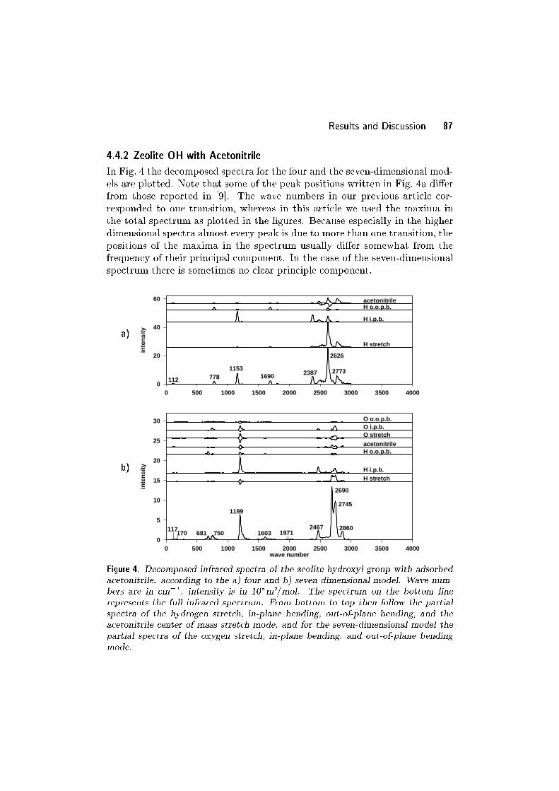
Results and Discussion 87
4.4.2 Zeolite OH with Acetonitrile
In Fig. 4 the decomposed spectra for the four and the seven-dimensional mod-
els are plotted. Note that some of the peak positions written in Fig. 4a di�er
from those reported in [9]. The wave numbers in our previous article cor-
responded to one transition, whereas in this article we used the maxima in
the total spectrum as plotted in the �gures. Because especially in the higher
dimensional spectra almost every peak is due to more than one transition, the
positions of the maxima in the spectrum usually di�er somewhat from the
frequency of their principal component. In the case of the seven-dimensional
spectrum there is sometimes no clear principle component.
a)
0
20
40
60
0 500 1000 1500 2000 2500 3000 3500 4000
inte
nsi
ty
H stretch
H i.p.b.
H o.o.p.b.acetonitrile
112 7781153
1690 2387
2626
2773
b)
0
5
10
15
20
25
30
0 500 1000 1500 2000 2500 3000 3500 4000
inte
nsi
ty
wave number
H stretchH i.p.b.
H o.o.p.b.acetonitrileO stretchO i.p.b.O o.o.p.b.
117170 681 750
1199
197116032467
2690
2745
2860
Figure 4. Decomposed infrared spectra of the zeolite hydroxyl group with adsorbed
acetonitrile. according to the a) four and b) seven-dimensional model. Wave num-
bers are in cm�1 , intensity is in 105m2=mol. The spectrum on the bottom line
represents the full infrared spectrum. From bottom to top then follow the partial
spectra of the hydrogen stretch, in-plane bending, out-of-plane bending, and the
acetonitrile center of mass stretch mode, and for the seven-dimensional model the
partial spectra of the oxygen stretch, in-plane bending, and out-of-plane bending
mode.

88 Chapter 4: Six and Seven-Coordinate Cluster Models
The decomposed spectrum of the four-dimensional calculation (Fig. 4),
clearly shows the interaction between the hydrogen stretch and the hydrogen
in-plane bending overtone. The in-plane bending mode has peaks on both
sides of the `Fermi dip' at ca. 2600 cm�1, whereas the stretch is predomi-
nantly present on the high frequency side. The acetonitrile stretch interacts
almost exclusively with the hydrogen stretch mode, causing a broadening of
approximately 300 cm�1.
In the four-dimensional spectra the following important transitions are
visible. At 112 cm�1 the fundamental acetonitrile center of mass stretch is
found. The out-of-plane hydrogen bending and its overtone are visible at
778 cm�1 and 1690 cm�1 respectively. At 1153 cm�1 we �nd the in-plane
hydrogen bending mode, its overtone is at 2387 cm�1. All these transitions
can be readily identi�ed from the partial spectra plotted in Fig. 4a. The
in-plane bending overtone at 2387 cm�1 has some slight interaction with the
hydrogen stretch and the main hydrogen stretch peak at 2626 cm�1 shows
substantial interaction with the in-plane bending overtone. This follows from
looking at the coeÆcients of the basis functions of the involved states, and
also from the partial spectra in Fig. 4a. The interaction between the in-plane
bending overtone and the hydrogen stretch is a Fermi resonance. This is an
interaction between two vibrational states that approximately have the same
energy, not caused by the symmetry of the molecule. The peak at 2773 cm�1
represents a combination band of the hydrogen stretch and the acetonitrile
center of mass stretch mode. From the partial acetonitrile stretch spectrum
it can be seen that the acetonitrile stretch interacts with all modes where the
hydrogen stretch mode is involved.
Combining the information from the coeÆcients of basis functions in the
wave functions, and the decomposition of the spectrum, we made the follow-
ing attribution of peaks in the seven-dimensional spectrum. The acetonitrile
stretch mode is found at 117 cm�1. The small peak at 170 cm�1 can be at-
tributed to the oxygen out-of-plane bending. The peaks at 685 cm�1 and 750
cm�1 are due to hydrogen in-plane-bending and oxygen out-of-plane bend-
ing modes respectively. The hydrogen in-plane bending mode is found at
1199 cm�1, and clearly enhanced in intensity compared to the spectrum with-
out acetonitrile. At 1603 cm�1 there is the hydrogen out-of-plane bending
mode overtone, and at 1971 cm�1 a small peak which is due to a combined
excitation of both the hydrogen and the oxygen in-plane bending modes can
be observed. Then from 2467 cm�1 to 2860 cm�1 there is the Fermi reso-
nance region. The peak at 2467 cm�1 is mainly due the hydrogen in-plane
bending overtone. The peaks at 2690 cm�1, 2745 cm�1 and 2860 cm�1 all
contain important contributions from both the hydrogen stretch and the in-
plane bending modes.

Results and Discussion 89
The seven-dimensional spectrum displays a somewhat clearer dip in the
Fermi resonance region than the four-dimensional spectrum. Also, the Fermi
region is slightly shifted to higher frequency, however leaving the dip around
the experimentally observed 2600 cm�1. The shift is smaller than the upward
shift of the hydroxyl group without acetonitrile, comparing three and six-
dimensional computations. This means that the overall calculated shift of the
hydroxyl stretch frequency upon acetonitrile absorption increases if one takes
into account the movements of the oxygen atom of the hydroxyl group.
The decomposition of the seven-dimensional spectrum is much less clear
than that of the other spectra. This is partly due to the anharmonic coupling
between the coordinates that we employed, which implies that it is impossi-
ble to assign infrared peaks to one single mode. Another factor is that the
number of excited states that should be included in the decomposition to ac-
count for the observed absorption intensity is much greater than for the other
spectra. The number of excited states actually included is however limited by
computational resources.
Fig. 5 shows a comparison between our six and seven-dimensional models
and an experimental di�erence spectrum. In this �gure the infrared spectrum
of a sample of HY is subtracted from the same sample after absorption of
acetonitrile [4]. We compare it with the di�erence between our calculated
spectra of the seven and six-dimensional models.
There is good agreement on the position of the Fermi resonance `dip' be-
tween experiment and our calculations. Also the fact that the low frequency
band is smaller in intensity than the high frequency band is re ected in the
calculation. What is clearly lacking in the calculated is overall width of the
A,B-dyad. Furthermore the correspondence of the two peaks in the free hy-
droxyl stretch region is deceptive. In the experimental spectrum the lower
frequency `free' hydroxyl band is due to a hydroxyl that forms a weak hy-
drogen bridge in HY. The low frequency band in the calculated spectrum in
this region represents the free hydroxyl stretch mode, and corresponds to the
higher frequency band in the experimental spectrum. The highest frequency
band in the calculated spectrum corresponds to a hot band (vide supra) that
is not present in the experimental spectrum, and presumably an artifact of
the cluster model and limited number of coordinates we used.

90 Chapter 4: Six and Seven-Coordinate Cluster Models
1500 2000 2500 3000 3500 4000wave number
Figure 5. Experimental (top) and calculated (bottom) infrared di�erence spectrum.
Wave numbers are in cm�1 . The experimental spectrum is the di�erence between
a spectrum of a HY sample loaded with acetonitrile, and one without acetonitrile.
The calculated spectrum is the di�erence between the calculated spectra for the
six and seven-dimensional models discussed in this paper. The dotted vertical line
indicates the `Fermi dip'. The sharp peaks around 2300 cm�1 in the experimental
spectrum are due to acetonitrile CH vibrations, and cannot be reproduced in our
model, where acetonitrile is modelled as rigid.
4.4.3 Interpretation of the A,B-Spectrum
The physical picture that is used in the explanation of the A,B-spectra in
several empirical models is based on a model that assumes a very strong
coupling � between the acidic hydroxyl stretch mode and the intermolecular
stretch mode of the adsorbed base with respect to the hydroxyl[6{8]. We
call this model I. In a discrete level model this means that combination and
di�erence bands of the hydroxyl stretch mode with many of the overtones of
the intermolecular stretch modes determine the band width. The coupling �0
between the hydroxyl stretch and the in-plane bending overtone in this model
is relatively weak compared to �.
There is however an alternative explanation of the same type of spectrum
possible, with � � �0 (model II). In this model the overall band width is
controlled by the coupling parameter �0 of the hydroxyl stretch and the in-
plane bending mode.
In previous discussions model I has been adopted, because it agrees with
the empirical law that the half-width of a shifted OH stretch band equals
approximately 34of the shift itself ([29] and references therein). This relation-
ship holds well for a number of experimental data, if for A,B-band systems
the half-width of the shifted hydroxyl stretch bands is taken to be the overall
width of the A,B-system.
However, our calculations point in the direction of a situation between
the extremes presented by model I and model II. From Fig. 4 we deduce
values of � � 200 cm�1 and �0 � 230 cm�1. The value of � for model I would
Conclusions 91
need to be approximately 800 cm�1. Although the potential energy surface
we employed leaves room for some improvement, we do not think a better
surface would give a signi�cantly di�erent result. For model II a value of �
approximately 300 cm�1 would suÆce to explain the same spectrum. If the
hydroxyl stretch mode in our model is shifted slightly downwards, peak A in
Fig. 4 would broaden, and reproduce the width of the experimental spectrum.
4.5 Conclusions
Using a six coordinate vibrational model for the bridged OH group in a zeo-
lite, we compute a value of 3522 cm�1 for the OH stretch frequency, which is
only 2.4% below the experimental value. Vibrational models with three coor-
dinates yield a value of 3375 cm�1, which is o� by 6.5%. The improvement in
the six dimensional computation is due to the coupling of the low frequency
oxygen modes with the hydrogen modes.
In the computed infrared spectrum of a zeolite bridged OH with adsorbed
acetonitrile the dip indicating Fermi resonance is at the same position as in
the experimental spectrum. In experimental spectra the position of the dip is
rather independent of the strength of the adsorbed base, so we can conclude
that the cluster model describes the zeolite bridged OH well. The computed
shift of the OH band however is too small, indicating that the interaction be-
tween the OH group and the acetonitrile molecule is not described suÆciently
by the used potential. Factors of importance are the quality description of the
hydrogen bridge by the used density functional, and the lack of interaction
with the zeolite wall in our model.
The general shape of the computed seven-dimensional spectrum is not
smooth enough. More vibrational modes will be needed to get a better ap-
proximation of the experimental spectrum. The method we used in the current
work is not suited to higher dimensional models.
Our calculations indicate that it is possible to interpret A,B-type of Fermi
resonance spectra with a coupling of the hydroxyl stretch with the stretch
mode of the adsorbed base of the order of 300 cm�1, if the coupling between
the hydroxyl stretch and in-plane bending overtone modes is considered to
be of the order of 300 cm�1, i.e., approximately the width of one of the A,B
bands appearing in the infrared spectrum.
Acknowledgement
This work has been performed under the auspices of NIOK, the Netherlands
Insitute for Catalysis research, Lab Report No. TUE{98{5{07.

92 Chapter 4: Six and Seven-Coordinate Cluster Models
References
[1] A. Zecchina, F. Geobaldo, G. Spoto, S. Bordiga, G. Ricchiardi, R. Buz-
zoni, and G. Petrini; J. Phys. Chem., \FTIR Investigation of the Forma-
tion of Neutral and Ionic Hydrogen-Bonded Complexes of H-ZSM-5 and
H-Mordenite with CH3CN and H2O: Comparison with the H-NAFION
Superacidic System", 100, 16584{16599 (1996).
[2] K. M. Neyman, P. Strodel, S. Ph. Ruzankin, N. Schlensog, H.
Kn�ozinger, and N. R�osch; Catal. Lett., \N2 and CO molecules as probes
of zeolite acidity: an infrared spectroscopy and density functional inves-
tigation", 31, 273{285 (1995).
[3] M. Bonn, M. J. P. Brugmans, A. W. Kleyn, and R. A. van Santen;
Chem. Phys. Lett., \Enhancement of the vibrational relaxation rate of
surface hydroxyls through hydrogen bonds with adsorbates", 233, 309{
314 (1995).
[4] A. G. Pelmenschikov, R. A. van Santen, J. J�anchen, and E. Meijer;
J. Phys. Chem., \CD3CN as a Probe of Lewis and Br�nsted Acidity of
Zeolites", 97, 11071{11074 (1993).
[5] A. G. Pelmenschikov, J.H.M.C. van Wolput, J. J�anchen, and R.A.
van Santen; J. Phys. Chem., \(A,B,C) Triplet of Infrared OH Bands of
Zeolite H-Complexes", 99, 3612{3617 (1995).
[6] J. C. Evans, and N. Wright; Spectrochim. Act., \A Peculiar E�ect in the
Infrared Spectra of Certain Molecules", 16, 352{257 (1960).
[7] R. .A van Santen; Recl. Trav. Chim. Pays-Bas, \Fano coupling in
perturbed solid acid hydroxyls", 113, 423{425 (1994).
[8] L. Kubelkov�a, J. Kotrla, and J. Flori�an; J. Phys. Chem., \H-Bonding
and Interaction of Acetonitrile Neutral and Pyridine Ion-Pair Surface
Complexes in Zeolites of Various Acidity: FTIR and ab Initio Study",
99, 10285{10293 (1995).
[9] E. L. Meijer, R. A. van Santen, and A. P. J. Jansen; J. Phys. Chem.,
\Computation of the Infrared Spectrum of an Acidic Zeolite Proton In-
teracting with Acetonitrile", 100, 9282{9291 (1996).
[10] A. D. Becke; J. Chem. Phys., \Density-functional thermochemistry. III.
The role of exact exchange.", 98, 5648{5652 (1993).
[11] A. D. Becke; Phys. Rev. A, \Density-functional exchange-energy approx-
imation with correct asymptotic behavior", 38, 3098{3100 (1988).
[12] C. Lee, W. Wang, and R. G. Parr; Phys. Rev. B, \Development of the
Colle-Salvetti correlation-energy formula into a functional of the electron
density", 37, 785{789 (1988).
References 93
[13] S. H. Vosko, L. Wilk, and M. Nusair; Can. J. Phys., \Accurate spin-
dependent electron liquid correlation energies for local spin density cal-
culations: a critical analysis", 58, 1200{1211 (1980).
[14] M. J. Frisch, G. W. Trucks, H. B. Schlegel, P. M. W. Gill, B. G.
Johnson, M. W. Wong, J. B. Foresman, M. A. Robb, M. Head-
Gordon, E. S. Replogle, R. Gomperts, J. L. Andres, K. Raghavachari,
J. S. Binkley, C. Gonzalez, R. L. Martin, D. J. Fox, D. J. Defrees, J.
Baker, J. J. P. Stewart, and J. A. Pople; Gaussian 92/DFT, Revision
F.2; Gaussian, Inc., Pittsburgh PA, 1993
[15] W. J. Hehre, R. F. Stewart, and J. A. Pople; J. Chem. Phys., \Self-
Consistent Molecular-Orbital Methods. I. Use of Gaussian Expansions of
Slater-Type Atomic Orbitals", 51, 2657{2664 (1969).
[16] R. Krishnan, J. S. Binkley, R. Seeger, and J. A. Pople; J. Chem.
Phys., \Self-Consistent Molecular-Orbital Methods. XX. A basis set for
correlated wave functions", 72, 650{654 (1973).
[17] T. Clark, J. Chandrasekhar, G. W. Spitznagel, P. v. R. Schleyer,
J. Comp. Chem., \EÆcient Di�use Function-Augmented Basis Sets for
First-Row Elements, Li{F", 4, 294{301 (1982).
[18] D. J. Defrees, and A. D McLean; J. Comp. Chem., \Ab Initio Determi-
nation of the Proton AÆnities of Small Neutral and Anionic Molecules",
7, 321{333 (1986).
[19] M. S. Gordon, J. S. Binkley, J. A. Pople, W. J. Pietro, and W. J.
Hehre; J. Am. Chem. Soc., \Self-Consistent Molecular-Orbital Methods.
22. Small Split-valence Basis-Sets for Second-Row Elements", 104, 2797{
2803 (1982).
[20] W. J. Hehre, R. Ditch�eld, and J. A. Pople; J. Chem. Phys., \Self-
ConsistentMolecular-OrbitalMethods. XII. Further Extensions of Gauss-
ian-Type Basis Sets for Use in Molecular-Orbital Studies of Organic
Molecules", 56, 2257{2261 (1971).
[21] M. M. Francl, W. J. Pietro, W. J. Hehre, J. S. Binkley, M. S. Gor-
don, D. J. Defrees, and J. A. Pople; J. Chem. Phys., \Self-Consistent
Molecular-Orbital Methods. XXIII. A Polarization-Type Basis Set for
Second Row Elements", 77, 3654{3665 (1986).
[22] P. C. Hariharan, and J. A. Pople; Theor. Chim. Acta, \The In uence of
Polarization Functions on Molecular-Orbital Hydrogenation Energies.",
28, 213{222 (1973).
[23] W. H. Press, B. P. Flannery, S. A. Teukolsky, and W. T. Vetterling;
Numerical Recipes in C, The Art of Scienti�c Computing; chap. 2.9, Cam-
bridge University Press, Cambridge, 1988.
[24] E. B. Wilson, Jr., J. C. Decius, and P. C. Cross; Molecular Vibrations;
Mc-Graw-Hill, New York, Toronto, London, 1955.

94 Chapter 4: Six and Seven-Coordinate Cluster Models
[25] E. B. Wilson, Jr., J. C. Decius, and P. C. Cross; Quantum Mechanics;
chap. XII, John Wiley & Sons, New York, 1955.
[26] L. Pauling, and E. B. Wilson; Introduction to Quantum Mechanics;
chap. XI, McGraw-Hill, 1935.
[27] J. G. Lewis; Algorithms for sparse matrix eigenvalue problems; chap. 3.4,
Stanford University, Department Computer Science, Stanford, 1977.
[28] B. N Parlett; The Symmetric Eigenvalue Problem; Prentice-Hall, Engle-
wood Cli�s, NJ, 1980.
[29] G. C. Pimentel, and A. L. McClellan; The Hydrogen Bond; chap. 3,
W. H. Freeman and Company, San Francisco and London, 1960.
5Cluster versus Embedded Model
Abstract
The infrared spectrum of a Br�nsted acidic hydroxyl in a zeolite, with and
without an adsorbed molecule of acetonitrile, has been studied with quantum-
chemical methods, and taking into account anharmonicity of the potential en-
ergy surface. This study extends earlier papers on the subject by focusing on
the validity of the cluster model that has been used to model the zeolite. We
compare a bare cluster model with an embedded cluster model, in which the
surroundings of the zeolite acidic site are modelled through molecular mechan-
ics, while the site itself and the adsorbate are treated quantum-chemically, at
the Hartree-Fock level. The embedding has virtually no e�ect on the cal-
culated infrared spectrum of the bare acidic hydroxyl. The up-shift of the
in-plane bending overtone upon adsorption of acetonitrile is more pronounced
in the embedded cluster than in the bare cluster. As a consequence the exper-
imentally found Fermi resonance is also apparent in the calculated spectrum
of the embedded cluster with acetonitrile, where it is absent in the calculated
spectrum of the bare cluster with acetonitrile. It is necessary to take into ac-
count anharmonicities to be able to reproduce the Fermi resonance spectrum.
Reproduced in part from E. L. Meijer, A. H. de Vries, R. A. van Santen,
P. S. Sherwood, and A. P. J. Jansen: \The Calculation of the Infrared Spec-
trum of an Acidic Zeolite OH with Adsorbed Acetonitrile: Cluster versus
Embedded Model", submitted for publication in J. Phys. Chem. A. Unpub-
lished work copyright 2000 American Chemical Society.
96 Chapter 5: Cluster versus Embedded Model
5.1 Introduction
Zeolites are crystalline materials consisting mainly of SiO4 tetrahedra that
are linked together through sharing of oxygen atoms. Many di�erent crystal
structures exist with channels and cages of molecular dimensions (4{12�A). In
most zeolites a fraction of the silicon atoms is replaced by aluminium atoms.
The negative charge this introduces into the lattice is balanced by cations,
often protons attached to the oxygen atoms that form the bridge between
a silicon and an aluminium atom. The resulting bridging hydroxyl exhibits
strong Br�nsted acidity. The combination of the Br�nsted acidic sites and
micro-pores of well-de�ned dimensions makes zeolites suitable catalysts for a
range of reactions.
In the infrared spectrum of a zeolite, the bridged hydroxyl stretch mode is
observed in the range 3605{3615 cm�1. If a weakly basic molecule is adsorbed
on the hydroxyl, the stretch frequency shifts down to lower values. Acetonitrile
is among the strongest basic molecules that only just fail to abstract the
proton from the acidic hydroxyl in a zeolite. The infrared spectrum of an
acidic hydroxyl disturbed by acetonitrile is more complicated than spectra
observed with weaker bases. The OH stretch mode shifts downward by 800 to
1200 cm�1, and splits into two very broad bands, often referred to as the A,B-
dyad. Sometimes a third band, denoted `C' is seen at yet lower frequencies.
Conclusive experimental evidence exists that these bands are due to one single
type of complex, where acetonitrile is hydrogen bonded to the Br�nsted acidic
OH. [1{3]
The characteristic splitting of the shifted hydroxyl stretch band into the
A,B-dyad is caused by Fermi resonance between the OH stretch mode (�) and
the overtone of the in-plane OH bending (Æ), where the plane referred to is
the plane in which the Si{O{Al atoms of the Br�nsted site lie.
In earlier work we tried to compute the infrared spectrum from �rst
principles,[4, 5] using a cluster model of the zeolite, and describing the acidic
hydroxyl with three [4] and six [5] degrees of freedom, respectively. The
present work extends on the simpler three-dimensional model, not by adding
more coordinates, but embedding the zeolite cluster model in a molecular
mechanics environment.

Computational Details 97
5.2 Computational Details
5.2.1 The Calculation of the Cluster Potential
The calculations presented in this paper were performed as an extension of an
earlier study, which employed a mixed basis set.[4] The embedded calculations
employ a 6-31G*[6{9] basis set throughout. To make a proper comparison,
we repeated the cluster calculations of Ref. [4] at the Hartree Fock level using
the 6-31G* basis set.
A (HO)3Si(OH)Al(OH)3 cluster was optimized at the Hartree-Fock level
in a 6-31G* basis set. During the optimization a mirror plane was maintained
through the Si{(OH){Al atoms of the cluster to reduce the number of points
that were necessary for the potential energy surface. The formation of internal
hydrogen bridges between the terminal OH groups was prevented by �xing the
H{O{Si and H{O{Al angles to tetrahedral angles, and forcing the H{O{Si{
Oc and H{O{Al{Oc atoms for each terminal OH group to stay in one plane,
where Oc denotes the central oxygen atom of cluster.
We derived a three-dimensional potential energy and dipole surface for
the hydrogen atom of the acidic OH group of the optimized cluster as follows.
A grid was constructed with OH distances of 0.8, 0.9, 1.0, 1.1, and 1.4 times
the equilibrium OH distance. At each distance the hydrogen atom was bent
towards the aluminium atom by an angle � of 0Æ, 7.5Æ, 20Æ, and 60Æ, and
subsequently rotated around the axis de�ned by the equilibrium OH bond by
an angle � of 0Æ, 45Æ, 90Æ, 135Æ, and 180Æ. Taking into account the symmetry
plane, the energies and dipoles of the geometries with � = 225Æ, 270Æ, and
315Æ could be inferred from the 135Æ, 90Æ, and 45Æ points, respectively.
For the infrared spectrum with acetonitrile, a molecule of acetonitrile was
added to the optimized zeolite cluster. Acetonitrile was adsorbed in the mirror
plane of the cluster, with the CN group pointing towards the OH group, and
one hydrogen atom of the CH3 group in the mirror plane on the side of the
silicon atom in the zeolite cluster. This cluster was optimized keeping the
mirror plane, and �xing the terminal OH groups at the positions they had in
the optimized bare zeolite cluster.
From the optimized complex we derived four-dimensional potential en-
ergy and dipole surfaces. For �ve positions of the acetonitrile molecule, where
it was shifted along its C{C�N axis by �0:5�A, �0:15�A, 0�A, 0.15�A, and0.5�A, a grid of acidic hydrogen positions was constructed in the same fashion
as for the bare zeolite. The internal coordinates of acetonitrile were kept �xed
in this procedure.
All Hartree Fock calculations for the cluster model were performed with
the Gaussian 92/DFT program package.[10]
98 Chapter 5: Cluster versus Embedded Model
The potential energy points were �tted with fourth order polynomials.
For the �t each point i was attributed a weight wi, so that points of lower
potential energy contribute more to the �t:
wi �e�fviPNj e
�fvj(1)
In this expression vi is the potential energy of point i, N the number of points,
and f a positive factor that determines the relative weight of the points. For
all calculations in this paper we used f = 125Eh�1, to produce a root mean
square error smaller than 1 � 10�3Eh. The energies computed for the grid
were in an interval of approximately 0.2Eh. The �ts were performed with
singular value decomposition, in order to remove near-degeneracy errors.
The same �t weights wi were used to �t the x-, y-, and z-components of
the dipoles of the geometries computed for the potential energy surface with
polynomials.
5.2.2 The Calculation of the Embedded Potential
The embedded cluster calculationswere performed as follows. A �nite siliceous
cluster was cut out from the ZSM-5 crystal structure.[11] The cut-out was
made by including all atoms within a 35 Bohr radius from a T2 Si; in all,
this cluster comprised ca. 1500 atoms. The central T2-site Si was replaced by
Al and a H-atom was added to make up for the charge defect. The H-atom
was attached to an O2-oxygen, as this was found to be the most favourable
position in an earlier study.[12] The geometries of the free Br�nsted acid site
and the site with acetonitrile adsorbed on it were optimized within the hybrid
QM/MM scheme, allowing full relaxation of the adsorbate and the back-bone
atoms within �ve bonds from the Al-atom. Three- and four-dimensional po-
tential energy and dipole surfaces for the Br�nsted site and the adsorption
complex were generated in the same way as described for the bare clusters,
except that for the embedded clusters no mirror symmetry was used.
The QM fragment was chosen to be a 5T-cluster, including the Al-atom,
the four O-atoms bound to Al, and the four Si-atoms bound to those O-
atoms. Comparison of results from periodic Hartree-Fock (HF) calculations
with embedded calculations of the same system has shown that a cluster with
�ve T atoms is the minimum size cluster that can be used to represent the
electrostatic potential at the central site accurately. The four Si-atoms were
terminated by H-atoms to satisfy the valence of the dangling bonds. The
H-atoms were restrained to lie on the Si-O bond, and the Si-H distance was
�xed to 1.5 Angstrom. The choice for termination with H atoms, instead of
with OH groups as we did in earlier studies, was determined by the experience

Computational Details 99
that Si-H termination reproduces a periodic HF potential in the center of the
QM region better than Si-OH termination.
The basis-set used on the QM fragment in all embedded cluster calcu-
lations was the 6-31G* basis set of GAMESS-UK [13], and all calculations
were performed at the Hartree-Fock level only. The embedding calculations
were run through the ChemShell package[14] using the GAMESS-UK code for
obtaining the energy and gradient for the QM fragment, and routines taken
from DL-POLY [15] to calculate the energy and gradient for the MM fragment
and the relevant QM/MM interaction terms.
The total energy for the QM/MM system consists of three main parts,
the MM energy of the MM atoms of the zeolite EMM(zeolite), the QM energy
of the QM cluster with the terminating hydrogen atoms EQM and the MM
interaction terms of the MM atoms with the QM region EMM(interaction).
EQM=MM = EMM(zeolite)+ EMM(interaction)+EQM (2)
The force-�eld used for the MM interactions was the aluminosilicate force-
�eld derived from ab-initio HF calculations by Hill and Sauer.[16] This force
�eld is a `consistent force �eld' (CFF) that contains terms for bonds, angles,
torsions, out-of-plane movements, and couplings between those terms, and
non-bonding terms. The MM potential energy in this model is given by
EMM(zeolite) = E(bonds) + E(angles) +E(torsions) +E(out-of-plane)
+ E(bond{bond) + E(angle{angle) + E(bond{angle)
+ E(angle{angle{torsion) +E(non-bond) (3)
E(non-bond) =Xi>j
qiqj
�rij
+Xi>j
Aij
r9ij
(4)
The non-bonding terms consist of the electrostatic energy due to atomic
charges qi (where the dielectric constant � has been set to 1), and a repulsive
term determined by the Aij coeÆcient. Both non-bonding terms are a func-
tion of the distance rij between two MM atoms. The energy of the MM part
of our system is computed according to Eq. 3.
The charges on the MM-atoms were altered from 0.52 on Si and �0:26on O to 1.2 on Si and �0:6 on O. The reason for this is that the latter charges
are better in reproducing the electrostatic potential as found in periodic HF
calculation in various zeolite pores.[17] Tests have shown that the use of these
altered charges does not a�ect the quality of the force-�eld signi�cantly. This
is to be expected because the force-�eld is a valence force-�eld where bond

100 Chapter 5: Cluster versus Embedded Model
stretch, angle bend, and torsion interactions between bonded atoms are pri-
marily responsible for the structure. The charges on the MM-atoms are as-
signed on a `per bond' basis. This means that an Si atom on the edge of the
cut-out gets a charge of +1:2 � n=4, where n is the number of bonds, and an
oxygen atom on the edge gets a charge of �0:6=2. This is done both on the
outer edges of the cut-out and on the MM/QM junction, to ensure that the
cut-out stays electrically neutral.
The minimum-energy conformations were obtained at the highest level of
embedding used in this study, which was similar to the electrostatic embedding
as described by Bakowies and Thiel.[18] At this level the electronic density of
the QM system is allowed to polarise under the in uence of the electrostatic
potential due to the MM cluster.
The electrostatic potential at the QM region is created by a set of point
charges at the MM atoms, augmented by 14 point charges situated just outside
the MM cluster. The 14 extra point charges are added to correct for the fact
that we use a �nite MM cluster, rather than embed in a periodic system.
They are the result of a �t to reproduce the periodic potential in the zeolite
cavity around the active site. The periodic potential is generated by point-
charges at the nuclei. The point-charge representation is derived from ab-initio
periodic HF calculations of the potential inside a range of zeolite pores already
mentioned.
MM-atoms close to the QM/MM junction may induce spurious QM po-
larisation, and therefore a simple procedure[19] is implemented to avoid such
artifacts. The charges on the O-atoms bound to the QM Si-atoms are shifted
to their MM Si-neighbours. At the MM Si-neighbours a dipole is introduced
to compensate the charge-shift.
At the highest embedding level we employed, the QM part of the total
energy (EQM) is the HF energy of the QM region of the system and the
terminating hydrogen atoms, where the electrostatic potential generated by
the MM part is included in the Hamiltonian. This electrostatic potential is due
to the MM atomic point charges, the 14 extra point charges mentioned above,
and the dipoles correcting for the shifted charges at the QM/MM junction.
We denote the QM energy with the MM electrostatic potential included in the
Hamiltonian as EQM(polarised), and the QM energy without this potential as
EQM(non-polarised).
The EMM(interaction) term in the total energy of the QM/MM system
contains terms that describe the QM/MM junction, where a chemical bond

Computational Details 101
between a MM oxygen with a QM silicon atom is modelled, and non-bonding
terms between the MM atoms and the QM atoms of the total system.
EMM(interaction) = Eint
MM(junction)
+Eint
MM(repulsion)
+Eint
MM(acetonitrile)�
+Eint
MM(electrostatic)
�(5)
The Eint
MM(junction) term contains the MM SiQM{OMM bond stretch terms,
which determines the length of the Si{O bond in a geometry optimization,
since the SiQM{HQM bond distances are kept �xed. The OQM{SiQM{OMM
angle is assumed to be adequately modelled by the bonds with the terminat-
ing H atoms of the QM zeolite cluster. The Eint
MM(repulsion) term is the non-
bonding, repulsive interaction described by thePAij=r
9ij term from Eq. 4,
where i runs over the MM atoms, and j over the QM atoms except the termi-
nating hydrogens. A schematic overview of some of the interactions near the
QM/MM junction is given in Fig. 1.
MM angle
junction atom
MM non-bond
Al
OSi
H
H
HOO
O
Si
H
H
H
O
O
O
O
OSi
MM stretch
QM angle
HO
Si
Figure 1. A schematic drawing of the interactions near the QM/MM junction. QM
atoms are drawn in boldface, MM atoms in thinner type. QM interactions are
indicated with thick lines, MM interactions are indicated with thin lines.
The Eint
MM(acetonitrile) term in Eq. 5 represents the non-bonded interactions
between the adsorbate (acetonitrile) and the silicate walls. These are not part
of the Hill and Sauer force-�eld. Parameters for C and H were taken from
the literature.[20] Parameters for N were derived from a general recipe based
on the Lennard-Jones parameterization in the CHARMM force-�eld[21], but
using di�erent polarisabilities, radii and number of valence electrons. We have
used the parameters from the DRF force-�eld,[22] which have been shown to
be applicable to a variety of systems. The parameters are listed in Tab. 1.

102 Chapter 5: Cluster versus Embedded Model
Table 1. Zeolite framework{substrate non-bonded interaction parameters.
Atom pair C6 (103 kJ bohr6/mol) C12 (10
6 kJ bohr12/mol)
Si{H �93:3262 5486.9096
O{H �23:2010 567.4308
Si{C �165:8753 17914.5380
O{C �45:1360 2219.5637
Si{N �75:8737 4085.1858
O{N �80:0788 1526.5521
The last term in Eq. 5, Eint
MM(electrostatic), is printed in square brack-
ets because it is not used in all the embedded potentials we computed. If
we include the MM electrostatic potential in the QM Hamiltonian as de-
scribed earlier, this term is set to zero, because it is part of EQM(polarised).
For further analysis of the results, we have computed potentials where the
MM electrostatic potential was not included in the QM Hamiltonian. Then
Eint
MM(electrostatic) contains the electrostatic interactions of the MM atomic
charges with the Si, Al, O, and acidic H atoms of the QM cluster, and a
correction for the way the charges at the QM/MM junction are dealt with in
EMM(zeolite). The QM Si atoms are assigned a charge of +1:2, the O atoms
a charge of �0:6, both like the MM atoms. The QM Al atom gets a charge of
+1:0, and the QM H atom of the acid OH group gets a charge of +0:2. The
procedure where the charges on the oxygen atoms at the QM/MM junction
were shifted to their nearest neighbours, which also a�ects the EMM(zeolite)
term in Eq. 2, has not been used for the potentials without the electrostatic
potential in the QM Hamiltonian. Additionally, if Eint
MM(electrostatic) is used,
the charge on the junction MM oxygen atoms is �0:6, instead of �0:6=2 whenthere is only one silicon neighbour with a MM point charge. For this discussion
we will formally assume that Eint
MM(electrostatic) contains terms to represent
these di�erences in EMM(zeolite). The atoms of acetonitrile do not contribute
to Eint
MM(electrostatic).
Four di�erent potentials were computed from the same geometries as the
fully embedded potential. Their contributing terms are listed in Tab. 2.
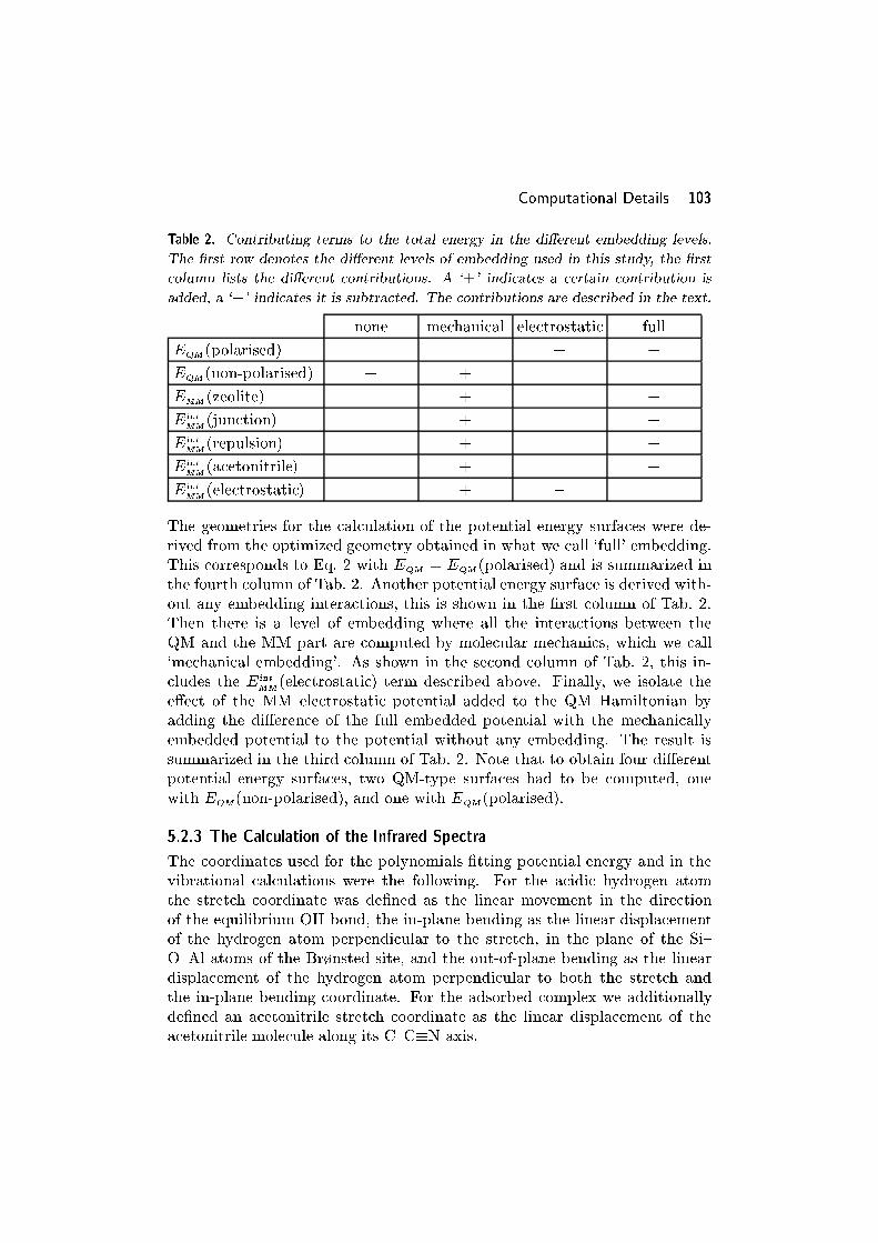
Computational Details 103
Table 2. Contributing terms to the total energy in the di�erent embedding levels.
The �rst row denotes the di�erent levels of embedding used in this study, the �rst
column lists the di�erent contributions. A `+' indicates a certain contribution is
added, a `�' indicates it is subtracted. The contributions are described in the text.
none mechanical electrostatic full
EQM(polarised) + +
EQM(non-polarised) + +
EMM(zeolite) + +
Eint
MM(junction) + +
Eint
MM(repulsion) + +
Eint
MM(acetonitrile) + +
Eint
MM(electrostatic) + �
The geometries for the calculation of the potential energy surfaces were de-
rived from the optimized geometry obtained in what we call `full' embedding.
This corresponds to Eq. 2 with EQM = EQM(polarised) and is summarized in
the fourth column of Tab. 2. Another potential energy surface is derived with-
out any embedding interactions, this is shown in the �rst column of Tab. 2.
Then there is a level of embedding where all the interactions between the
QM and the MM part are computed by molecular mechanics, which we call
`mechanical embedding'. As shown in the second column of Tab. 2, this in-
cludes the Eint
MM(electrostatic) term described above. Finally, we isolate the
e�ect of the MM electrostatic potential added to the QM Hamiltonian by
adding the di�erence of the full embedded potential with the mechanically
embedded potential to the potential without any embedding. The result is
summarized in the third column of Tab. 2. Note that to obtain four di�erent
potential energy surfaces, two QM-type surfaces had to be computed, one
with EQM(non-polarised), and one with EQM(polarised).
5.2.3 The Calculation of the Infrared Spectra
The coordinates used for the polynomials �tting potential energy and in the
vibrational calculations were the following. For the acidic hydrogen atom
the stretch coordinate was de�ned as the linear movement in the direction
of the equilibrium OH bond, the in-plane bending as the linear displacement
of the hydrogen atom perpendicular to the stretch, in the plane of the Si{
O{Al atoms of the Br�nsted site, and the out-of-plane bending as the linear
displacement of the hydrogen atom perpendicular to both the stretch and
the in-plane bending coordinate. For the adsorbed complex we additionally
de�ned an acetonitrile stretch coordinate as the linear displacement of the
acetonitrile molecule along its C{C�N axis.
104 Chapter 5: Cluster versus Embedded Model
The Hamiltonian employed in the vibrational calculations has the follow-
ing form:
H =1
2
DXi=1
DXj=1
(M�1)ijpipj +X
�1;:::;�D
a�1;:::;�D
DYi=1
q�ii ; with 0 �
DXi=1
�i � N
(6)
In this expression the D is the number of dimensions, qi are the spatial co-
ordinates with conjugated momenta pi, M�1 is the inverse mass matrix, and
a�1;:::;�D are the coeÆcients of the polynomial representing the potential en-
ergy. The polynomials used to �t the potential energy in this paper have all
been of fourth order, which corresponds with N = 4 in Eq. 6.
The wave functions were expanded in products of one-dimensional har-
monic eigenfunctions (Hermite functions).[23]
(q1 : : : qD) =X
�1;:::;�D
c�1;:::;�D
DYi=1
�(�i)(qi) (7)
Here is the D-dimensional vibrational wave function, and �(�i)(qi) is the
normalized �thi order Hermite function of coordinate qi. The basis has been
truncated by specifying a maximum order �(max)
i for each coordinate, and
subsequently limiting the basis functions used to those that meet the following
condition:DXi=1
�i
�
(max)
i
� 1 (8)
In the computations described here �(max)
i = 12 for all the coordinates. For
the three- and four-dimensional dimensional calculations this yields basis sets
of 455 and 1820 functions respectively.
Infrared absorption intensities were computed using Fermi's golden rule
[24] and fractional Boltzmann occupation numbers at a given temperature.
The integrated absorption intensity Ai!f from initial level i to �nal level f
is given by
Ai!f =2�2�E
3�0h2c2
X�=x;y;z
��hij��jfi��2 e�Ei=kTPLj e
�Ej=kT(9)
In this expression Ai!f is de�ned for one particle per unit surface, integrated
over wave numbers and averaged over di�erent molecular orientations. �E is
the di�erence in energy between the normalized states jii and jfi, �0 is the
electrical permittivity of vacuum, h is Planck's constant, c is the speed of
Results and Discussion 105
light in vacuum, �x, �y, and �z are the components of the dipole operator,
Ej is the energy of vibrational level j, k is the Boltzmann constant, T is the
absolute temperature, and L is the number of levels taken into account.
In the calculation of matrix elements of the Hamiltonian and of the
dipole component operators, mechanical as well as electric anharmonicities
were taken into account. The vibrational calculations were carried out with
the AnharmND program written by E.L.M. For a more detailed discussion of
the method we refer to our previous papers on the subject. [4, 5]
5.3 Results and Discussion
The �gures of infrared spectra in this paper have been obtained by convo-
luting delta functions representing the calculated intensity and position for
the transitions, with Gaussian curves of half width 10 cm�1 and unity surface
area. As a consequence the surface area under the graphs correctly represents
the calculated integrated absorption intensity, whereas the peak widths are
arbitrary. The alternative of plotting spikes where the height represents the
absorption intensity is not suitable to display spectra with a high density of
peaks, like the infrared spectra with acetonitrile. All spectra have been com-
puted taking into account a Boltzmann distribution over the calculated states
at a temperature of 298.15K.
In the plotted infrared spectra we have printed the wave numbers of im-
portant transitions. For the spectra of the zeolite OH without acetonitrile
these numbers have been derived from di�erences between computed levels.
For the spectra of the zeolite OH with acetonitrile, there are many overlap-
ping hot bands, because higher excited states of the acetonitrile mode are
populated signi�cantly at room temperature. Therefore we have printed wave
numbers that correspond to the maxima in the plotted graphs. They represent
a weighted average for di�erent transitions that contribute to the peaks.
5.3.1 Basis Set E�ects
In previous work we have computed the infrared spectra of a zeolite OH with
or without acetonitrile adsorbed in a cluster approach.[4, 5] In this paper we
are comparing the results obtained from `bare' clusters with those we get from
embedded clusters. The mixed basis set we used before has high quality basis
functions on the central OH group and the nitrogen atom of acetonitrile (6-
311+G**), low quality functions on the terminal hydrogen atoms (STO-3G),
and 6-31G** on the other atoms of the cluster. For the embedded calculations
we have used 6-31G* throughout, which resulted in a smaller overall basis set.
Fig. 2 and Fig. 3 show the spectra as computed with bare clusters, with the
mixed and the balanced 6-31G* basis set respectively.
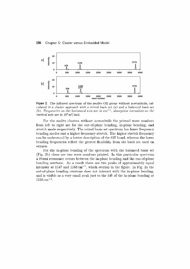
106 Chapter 5: Cluster versus Embedded Model
a)
0
10
20
0 500 1000 1500 2000 2500 3000 3500 4000
inte
nsi
ty
4781126 3779
b)
0
10
20
0 500 1000 1500 2000 2500 3000 3500 4000
inte
nsi
ty
wave number
539 11471163 3741
Figure 2. The infrared spectrum of the zeolite OH group without acetonitrile, cal-
culated in a cluster approach with a mixed basis set (a) and a balanced basis set
(b). Frequencies on the horizontal axis are in cm�1 , absorption intensities on the
vertical axis are in 105m2=mol.
For the zeolite clusters without acetonitrile the printed wave numbers
from left to right are for the out-of-plane bending, in-plane bending, and
stretch mode respectively. The mixed basis set spectrum has lower frequency
bending modes and a higher frequency stretch. The higher stretch frequency
can be understood by a better description of the OH bond, whereas the lower
bending frequencies re ect the greater exibility from the basis set used on
oxygen.
For the in-plane bending of the spectrum with the balanced basis set
(Fig. 2b) there are two wave numbers printed. In this particular spectrum
a Fermi resonance occurs between the in-plane bending and the out-of-plane
bending overtone. As a result there are two peaks of approximately equal
intensity at 1147 and 1163 cm�1, which overlap in the �gure. In Fig. 2a the
out-of-plane bending overtone does not interact with the in-plane bending,
and is visible as a very small peak just to the left of the in-plane bending at
1126 cm�1.

Results and Discussion 107
a)
0
10
20
0 500 1000 1500 2000 2500 3000 3500 4000
inte
nsi
ty
87776
1213
1672 25363220
3258
3363
b)
0
10
20
0 500 1000 1500 2000 2500 3000 3500 4000
inte
nsi
ty
wave number
90772
1221
1653 25533274
3357
3463
Figure 3. The infrared spectrum of the zeolite OH group with acetonitrile, calculated
in a cluster approach with a mixed basis set (a) and a balanced basis set (b). Fre-
quencies on the horizontal axis are in cm�1 , absorption intensities on the vertical
axis are in 105m2=mol.
For the zeolite cluster with adsorbed acetonitrile the wave numbers from
left to right refer to the acetonitrile stretch mode, the OH out-of-plane bending
and in-plane bending modes, followed by their respective �rst overtones, and
the OH stretch mode along with di�erence and combination modes with the
acetonitrile stretch. The upward shift of the bending modes is larger for the
mixed basis set, and the absolute frequency of the OH stretch is lower than for
the balanced basis set, although it was higher before acetonitrile adsorption.
Both the upward shift of the in-plane bending and the downward shift of
the OH stretch are indicative of the strength of the interaction between the
OH group and acetonitrile. The argument for using the enlarged basis set
on the acid OH group and N has been that it yields a better description of
the interaction between the zeolite OH group and acetonitrile.[4, 25, 25] From
Fig. 2 and Fig. 3 we conclude that it does exactly that.
5.3.2 Embedding E�ects
In Fig. 4 the spectra of the zeolite OH without acetonitrile from the embed-
ded cluster have been plotted, with di�erent levels of interaction between the
quantum mechanical cluster part (QM) and the molecular mechanics embed-
ding (MM). Fig. 4a represents the spectrum of the embedded cluster without
any interaction between QM and MM parts, Fig. 4b and 4c are the spectra
with only the mechanical embedding and with only the electrostatic interac-
tion respectively, and Fig. 4d is the spectrum of the embedded cluster with
all interactions between QM and MM parts.

108 Chapter 5: Cluster versus Embedded Model
a)
0
10
20
0 500 1000 1500 2000 2500 3000 3500 4000
inte
nsi
ty
4551066
3737
b)
0
10
20
0 500 1000 1500 2000 2500 3000 3500 4000
inte
nsi
ty
4551067
3737
c)
0
10
20
0 500 1000 1500 2000 2500 3000 3500 4000
inte
nsi
ty
4661126
3724
d)
0
10
20
0 500 1000 1500 2000 2500 3000 3500 4000
inte
nsi
ty
wave number
4661126
3724
Figure 4. The infrared spectrum of the zeolite OH group without acetonitrile, calcu-
lated in an embedded cluster approach with di�erent levels of interaction between
the quantum mechanical part and the molecular mechanics part. Spectrum (a) is
calculated without interaction between the QM and the MM part, (b) only has the
mechanical embedding interactions, (c) only has the electrostatic interaction of the
MM part, and (d) has all the interactions between the QM part and the MM part.
Frequencies on the horizontal axis are in cm�1 , absorption intensities on the vertical
axis are in 105m2=mol.
A comparison between Fig. 2b and Fig. 4a shows that the bending modes
have lower frequencies for the cluster used in the embedded calculations than
for the bare cluster used in the previous work.[4] For the in-plane bend the fact
that in the bare cluster the acidic OH group has an eclipsed con�guration with
respect to the terminating OH groups on Al and Si, whereas for the embedded
cluster it is staggered with respect to the SiH groups, could be o�ered as an
explanation for the di�erence in the in-plane bending frequency. There are
also di�erences in chemical composition between the bare and the embedded
cluster, and in the embedding the SiH bonds were �xed at a distance of
1.5�A. In a cluster in which the Si{H distances are optimized, they would be
somewhat smaller than the �xed distance of 1.5�A used here. It has been shown

Results and Discussion 109
that the acid strength of Si{H terminated aluminosilicate clusters is sensitive
to the Si{H distance.[12, 26, 26] This accounts for the lower frequencies in the
embedded cluster (Fig. 4a) compared to the bare cluster (Fig. 2b).
The di�erent parts of Fig. 4 reveal that almost all of the di�erence be-
tween the fully embedded spectrum (Fig. 4d) and the spectrum of the embed-
ded cluster without any interaction between QM and MM part (Fig. 4a) is
due to the electrostatic interaction of the QM part with the MM part. The ef-
fect of the mechanical embedding is negligible, because only the non-bonding
interaction terms in it can a�ect the computed infrared spectrum. These non-
bonding interactions between the acidic proton and the surrounding zeolite
are very small indeed.
To explain why the electrostatic interaction a�ects the in-plane bend sig-
ni�cantly more than the out-of-plane bend, we inspected two cross-sections of
the applied electrostatic potential. Fig. 5a shows contours of the electrostatic
potential in the region of the acid site for the optimized embedded cluster
with acetonitrile. The contours are shown at intervals of 0.0025 a.u., and a
cross-section is cut in the plane approximately containing the O{H and N{C
dipoles. For the free acid, embedded in the full potential, the electrostatic
potential over the site may be slightly di�erent, but not in a qualitative way.
Observing the curvature of the contours around the O{H dipole it can be
seen that the in-plane bend will be hindered by the electrostatic �eld: the
contours curve against the O{H dipole, thereby introducing an unfavourable
interaction when moving the O{H dipole in the O{Al{O plane.
Fig. 5b shows that the electrostatic potential almost curves along the
out-of-plane bend of the acid O{H group. As a result the added potential for
this mode is shallow and the e�ect on the frequency of the out-of-plane bend
is small.
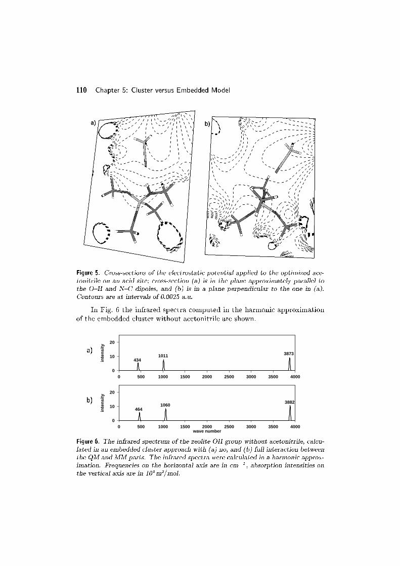
110 Chapter 5: Cluster versus Embedded Model
Figure 5. Cross-sections of the electrostatic potential applied to the optimized ace-
tonitrile on an acid site; cross-section (a) is in the plane approximately parallel to
the O{H and N{C dipoles, and (b) is in a plane perpendicular to the one in (a).
Contours are at intervals of 0.0025 a.u.
In Fig. 6 the infrared spectra computed in the harmonic approximation
of the embedded cluster without acetonitrile are shown.
a)
0
10
20
0 500 1000 1500 2000 2500 3000 3500 4000
inte
nsi
ty
4341011 3873
b)
0
10
20
0 500 1000 1500 2000 2500 3000 3500 4000
inte
nsi
ty
wave number
4641060
3882
Figure 6. The infrared spectrum of the zeolite OH group without acetonitrile, calcu-
lated in an embedded cluster approach with (a) no, and (b) full interaction between
the QM and MM parts. The infrared spectra were calculated in a harmonic approx-
imation. Frequencies on the horizontal axis are in cm�1 , absorption intensities on
the vertical axis are in 105m2=mol.

Results and Discussion 111
Comparing the harmonic spectrum in Fig. 6a with its anharmonic coun-
terpart in Fig. 4a, the OH stretch frequency is higher and the bending mode
frequencies are lower, but qualitatively the spectra are very much alike. Note
that anharmonicity does not always lower frequencies. The e�ect of the em-
bedding interactions between the QM and the MM part is larger for the
harmonic out-of-plane bend than for the anharmonic out-of-plane bend, but
smaller for the in-plane bend, which is more important for the Fermi-resonance
we seek to reproduce. The shift of the harmonic stretch due to the embedding
interactions has the opposite sign of that found in the anharmonic spectrum.
For the zeolite OH group with adsorbed acetonitrile the spectra of the
embedded clusters at di�erent levels of interaction are given in Fig. 7. Here
the di�erences are more pronounced than in the case without acetonitrile.
Firstly there is a clear e�ect of the di�erent cluster optimized in the em-
bedded approach (Fig. 7a) compared to the bare cluster approach (Fig. 3b).
The embedded cluster has a di�erent chemical composition, and it has been
optimized to mimic a site in an actual zeolite. This results in a cluster that
has a stronger interaction with acetonitrile than then bare cluster, which
is apparent in a number of peaks in the spectra. The bending modes are
higher in frequency for the embedded cluster. As a consequence the in-
plane bend overtone also is higher for the embedded cluster (2936 cm�1 vs.
2553 cm�1), and it comes closer to the OH stretch which is lower in the em-
bedded cluster.(3334 cm�1 vs. 3357 cm�1) This is the e�ect we are after; if the
in-plane bend overtone and the OH stretch coincide, Fermi resonance between
the two modes occurs. The acetonitrile stretch frequency is slightly higher in
Fig. 7a than in Fig. 3b (94 cm�1 vs. 90 cm�1), which also hints at a stronger
interaction.
In the comparison between the spectra computed from the bare cluster
with the embedded cluster without additional interactions (Fig. 2b vs. Fig. 4a,
and Fig. 3b vs. Fig. 7a), we �nd lower OH bend frequencies in the absence, and
higher OH bend frequencies in the presence of acetonitrile. Both di�erences
can be accounted for assuming that the embedded acetonitrile cluster is more
acidic than the bare cluster with the balanced basis set. The embedded cluster
can be more acidic because the residual negative charge can be spread over
a larger volume as the Al atom is surrounded by four O{SiH3 groups. As
pointed out in the paragraph on the clusters without acetonitrile, the �xed
SiH distances also play a role in the strength of the acid OH bond.
We have two indications that the embedded cluster with mechanical
and electrostatic interactions is more acidic than the (HO)3Si{(OH){Al(OH)3cluster. Firstly the adsorption energy of acetonitrile on the bare cluster is
�22:4 kJ=mol, and that on the embedded cluster is �76 kJ=mol. These num-bers include deformation energies of acetonitrile and the zeolite cluster; they
are not corrected for basis set superposition errors (BSSE). Secondly it has

112 Chapter 5: Cluster versus Embedded Model
been shown that there is a correlation between the barrier for H/D exchange
of methane and the proton aÆnity of a cluster.[26] A higher barrier for the
D/H exchange reaction corresponds to a lower proton aÆnity, which in turn
corresponds to a higher acidity. At Hartree-Fock level, the `trimer' cluster
used in Ref. 26 had a barrier of 230 kJ=mol with a 6-31G** basis set, and
the chemically identical cluster in Ref. 12 had a barrier of 250 kJ=mol with a
6-31G* basis set in the embedding scheme we also use in the present paper.
This indicates that the embedding renders the cluster more acidic.
a)
0
10
20
0 500 1000 1500 2000 2500 3000 3500 4000
inte
nsi
ty
94788
1460
1683 2936 3249
3334
3443
b)
0
10
20
0 500 1000 1500 2000 2500 3000 3500 4000
inte
nsi
ty
80 732
1426
28513302
3368
3460
c)
0
10
20
0 500 1000 1500 2000 2500 3000 3500 4000
inte
nsi
ty
101776
1620
1756
3276
3494
d)
0
10
20
0 500 1000 1500 2000 2500 3000 3500 4000
inte
nsi
ty
wave number
93773
1591
16453266
3436
Figure 7. The infrared spectrum of the zeolite OH group with acetonitrile, calcu-
lated in an embedded cluster approach with di�erent levels of interaction between
the quantum mechanical part and the molecular mechanics part. Spectrum (a) is
calculated without interaction between the QM and the MM part, (b) only has the
mechanical embedding interactions, (c) only has the electrostatic interaction of the
MM part, and (d) has all the interactions between the QM part and the MM part.
Frequencies on the horizontal axis are in cm�1 , absorption intensities on the vertical
axis are in 105m2=mol.
Haw et al.[27] have modelled the Br�nsted acid site in ZSM-5 replacing
the silicon atom on the T6 position with a cluster containing one aluminium

Results and Discussion 113
atom and two neighbouring silicon atoms. They have computed an interaction
energy of �56:1 kJ=mol at Hartree-Fock level without correction for BSSE.
The NH distance they �nd is 1.56�A, which is rather short compared to the
1.93�A we �nd for our bare cluster with balanced basis set, and 2.04�A for our
embedded cluster. It may well be that their cluster is somewhat too reactive
because they �xed all silicon, aluminium, and oxygen atoms at positions taken
from crystallographical data. These positions most likely do not correspond to
a minimum in energy for the method they used. Barbosa et al.[28] computed
interaction energies for acetonitrile with a zeolite cluster of �42:6 kJ=mol atHartree-Fock level, and �47:5 kJ=mol at DFT level without BSSE correction,
and of �38 kJ=mol at DFT level with full counterpoise correction.[29] The NH
distances they found were 1.88�A for Hartree-Fock and 1.73�A for DFT. Their
cluster contains two hydrogen terminated silicon atoms and one hydroxyl ter-
minated aluminium atom. The somewhat smaller NH distance and somewhat
larger adsorption energy compared to our bare cluster can be explained by
the di�erence in cluster, and the larger basis set they used.
Experimental heats of absorption have been measured for acetonitrile on
Br�nsted acidic groups in the range from �60 to �80 kJ=mol (depending onloading) in zeolite HY[30] and of �110 kJ=mol in H-ZSM-5.[31] Part of the
di�erence between these experimental values can be ascribed to the smaller
pore size of ZSM-5; measurements of adsorption heat of acetonitrile in silicious
ZSM-5 yield a value that is 10 kJ=mol larger than in silicious faujasite.[30] The
rest is probably due to the di�erence in Si/Al ratios. The ZSM-5 sample of
Ref.[31] has a Si/Al ratio of approximately 25, whereas the Si/Al ratio of the
HY sample of Ref.[30] is only 2.4. The acidic strength of Br�nsted sites in
zeolites decreases with higher aluminium content.
After correction for BSSE, the interaction energy of the bare cluster with
acetonitrile becomes �17:0 kJ=mol. This means the BSSE constitutes 24% of
the interaction energy. Since this is quite substantial we have done a few tests
to assess the e�ect of BSSE on computed frequencies. First we have computed
the interaction energy and the BSSE of the bare zeolite cluster with acetoni-
trile at equilibrium distance, and 0.15�A closer and further away. For these
three points we �tted the interaction energy and the counterpoise corrected
interaction energy with a second order polynomial. We derived that the coun-
terpoise correction decreases the harmonic vibration frequency by 3.3%, and
elongates the distance between the zeolite cluster and acetonitrile by 0.05�A.
The counterpoise corrected interaction energy at the displaced minimum is
�17:3 kJ=mol. Because the main interest of this article is in the vibrations
of the acidic OH group, we also checked the e�ect of a counterpoise correc-
tion one a one-dimensional stretch vibration of the acidic hydrogen atom in
the presence of acetonitrile at equilibrium distance. A fourth order potential
for the OH stretch was computed from points at 0.8, 0.9, 1.0, 1.1 and 1.4

114 Chapter 5: Cluster versus Embedded Model
times the equilibrium OH bond length. The counterpoise correction causes
a decrease in the computed anharmonic fundamental frequency of 0.6%, and
an increase of the expectation value of the OH distance of 0.04%. We con-
clude that counterpoise correction does not greatly in uence the computed
spectrum. Note that to apply a correction for BSSE rigorously, the cost of
computing a potential energy surface easily increases by a factor of three to
four. It is also not clear how to deal with dipole surfaces in a way that is
consistent with a counterpoise correction.
The two di�erent types of interaction between the QM and the MM part
have opposite e�ects on the spectrum of the zeolite OH with adsorbed acetoni-
trile. The e�ect of the mechanical embedding on this spectrum is noticeable,
because acetonitrile has signi�cant non-bonding interactions with the sur-
rounding zeolite. These interactions pull the acetonitrile molecule closer to
the zeolite wall, and away from the acidic proton. In Tab. 3 some expectation
values of atomic distances and angles are listed, and it can be seen that for
the embedded cluster with mechanical interactions, the ON and NH distances
are larger than for the embedded cluster without any interactions. The OH
distance of the acidic group on the other hand is shorter for the cluster with
mechanical interactions. These geometrical di�erences indicate that the em-
bedded cluster with mechanical interactions has a smaller interaction with ace-
tonitrile, and this is con�rmed by the di�erences between the spectra in Fig. 7a
and Fig. 7b: the OH stretch frequency goes up (3334! 3368 cm�1), and the
bending frequencies go down (788! 732 cm�1 and 1460! 1426 cm�1), i.e.,
all OH frequencies shift in the direction of the values they have in the spec-
trum without acetonitrile. Also the acetonitrile stretch frequency is smaller
in Fig. 7a than in Fig. 7b, in accordance with a smaller interaction.
Table 3. Expectation values for distances and angles between the oxygen and hy-
drogen atoms of the acid OH group, and nitrogen of the acetonitrile molecule, for
di�erent levels of embedding interactions included. The angle 6 (Al{O{N) has the
same value of 120.55Æ for all interaction levels. Distances are in �A, and angles in
degrees.
interactions rOH rON rNH 6 (Al{O{H) 6 (H{O{N) 6 (Al{O{Si{H)
none 0.98330 2.9177 2.0063 103.61 18.088 �173:26mechanic 0.97911 3.0001 2.0959 103.18 18.651 �173:73
electrostatic 0.98435 3.0452 2.1500 101.43 20.375 �173:84all 0.98131 3.1195 2.2311 101.05 20.974 �174:60
The electrostatic interaction a�ects the infrared spectrum in a similar
manner as the interaction with acetonitrile does; the OH stretch frequency
goes down, and the in-plane bending mode goes up. These are the same
tendencies seen in the spectra of the embedded cluster without acetonitrile.

Results and Discussion 115
The shifts are large enough to cause a Fermi resonance between the OH in-
plane bend overtone and the OH stretch. This is the phenomenon we were
trying to reproduce, and it is clearly visible in Fig. 7c.
The electrostatic potential of the zeolite lattice polarises both the OH
and the NC dipoles, which could lead to a stronger interaction. At the same
time however, both the ON and the NH distances increase (Tab. 3), which in
turn suggests a weaker interaction. If we assumed a stronger interaction, we
would expect this to cause an increase in frequency in both the in-plane and
the out-of-plane bend, because both bending modes misalign the OH dipole
with the NC dipole. This is not what we �nd: the in-plane bending mode
indeed goes up in frequency, but the out-of-plane bending mode goes down.
The changes in the infrared spectrum of the embedded cluster with ace-
tonitrile upon application of the zeolite electrostatic �eld can be explained by
the e�ect of electrostatic �eld itself on the acidic OH group, even if the inter-
action of the OH group with acetonitrile is slightly weaker. The electrostatic
�eld elongates the OH bond, which accounts for a lower stretch frequency. In
the same way as discussed earlier for the OH group, the electrostatic �eld af-
fects the in-plane bending mode stronger than the out-of-plane bending mode.
The in-plane bend goes up because of its misalignment with the electrostatic
�eld. The fact that the out-of-plane bend goes down after application of the
electrostatic potential in the case with acetonitrile present, whereas it goes
slightly up without acetonitrile, can be explained by a weakening of the inter-
action with acetonitrile upon application of the electrostatic �eld. Finally the
relatively high acetonitrile stretch frequency of 101 cm�1 in Fig. 7c should be
attributed to the electrostatic forces acting on the molecule (see Fig. 5), and
not to an increased interaction between the acidic site and acetonitrile.
The infrared spectrum calculated with all interactions included (Fig. 7d)
also exhibits a Fermi resonance pattern, but with more intensity at higher
wave numbers compared to the spectrum with only the electrostatic interac-
tion. The spectrum di�ers from the experimental spectra[1{3] in two impor-
tant ways. Firstly the frequency of the Fermi complex of bands is too high.
Experimentally the center of the AB-bands is at 2600 cm�1, whereas in Fig. 7c
it lies around 3300 cm�1. As shown before,[4] this can be largely attributed
to the shortcomings of Hartree-Fock, and it could be improved using DFT
for the potential energy surface instead. The second important di�erence be-
tween the computed spectrum and the experimental ones is the overall width
of the AB-bands. This is too small in the computed spectra, similar to our
earlier work without embedding.[4, 5] In our view there are two shortcomings
in our model that contribute to this discrepancy. The �rst one is the limited
number of vibrational modes that we have been able to take into accont. We
expect a `smoothing' e�ect of the coupling of more modes of the acetonitrile

116 Chapter 5: Cluster versus Embedded Model
molecule and of the zeolite lattice if they are taken into account in the vi-
brational calculations. Secondly we have shown that the interaction energy
between the zeolite and acetonitrile in our model is too small in comparison
with experiment. We expect the acetonitrile frequency to go up if the interac-
tion is better described, resulting in combination bands with the OH stretch
that are further apart than in the current model.
The analysis of the electrostatic and non-bonding e�ects is very interest-
ing and could be tested on other zeolite sites. We should look for larger pores
and sites at which the electrostatic �eld counters the OH and NC dipoles. It
is not immediately clear what will happen; the e�ects do not exactly cancel.
The electrostatic e�ect is especially interesting because it distinguishes be-
tween the out-of-plane bending and the in-plane bending modes. This could
be of importance for modelling an ABC-spectrum, where the C band is due
to interaction of the OH stretch with the out-of-plane bend overtone. A safe
prediction seems to be the that at a site with a parallel electrostatic �eld in
a small pore, the Fermi resonance will be stronger than what we found here,
because the non-bonding interactions will push the bending mode overtones
up.
a)
0
10
20
0 500 1000 1500 2000 2500 3000 3500 4000
inte
nsi
ty
93554
1437
3504
b)
0
10
20
0 500 1000 1500 2000 2500 3000 3500 4000
inte
nsi
ty
wave number
86
598
1532
3566
Figure 8. The infrared spectrum of the zeolite OH group with acetonitrile, calculated
in an embedded cluster approach with (a) no, and (b) full interaction between the
QM and MM parts. The infrared spectra were calculated in a harmonic approxima-
tion. Frequencies on the horizontal axis are in cm�1 , absorption intensities on the
vertical axis are in 105m2=mol.
In Fig. 8 spectra of the embedded cluster with acetonitrile computed with
the harmonic part of the potential are shown. A comparison of Fig. 8a with
Fig. 7a, and of Fig. 8b with Fig. 7d shows not only signi�cant di�erences in
frequencies, but also large qualitative di�erences between the harmonic and
the anharmonic spectra. The bending overtones that are prominent in the
anharmonic spectra are absent in the harmonic ones. The combination and

Conclusion 117
di�erence bands of the OH stretch and the acetonitrile stretch are also absent
in the harmonic spectrum. Clearly, to reproduce a Fermi-resonance spectrum
it is necessary to take anharmonicities into account.
5.4 Conclusion
The infrared spectrum of a zeolite OH with adsorbed acetonitrile is signif-
icantly in uenced by the environment of the acidic site. In an embedded
cluster model where only three hydrogen coordinates and one intermolecular
coordinate between acetonitrile and the acidic OH were taken into account,
the Fermi resonance pattern between the OH stretch and the in-plane bending
overtone can be reproduced.
It appears that for the site we have studied non-bonding interactions with
the zeolite lattice and the zeolite electrostatic potential have opposite e�ects
on the infrared spectrum. The non-bonding interactions compete with the
OH-acetonitrile interaction and weaken it, moving the spectrum away from
Fermi resonance. The electrostatic potential also weakens the OH-acetonitrile
interaction, but like the OH-acetonitrile interaction, it increases the in-plane
bend and decreases the stretching mode frequency, making Fermi resonance
occur in the spectrum. As a result Fermi resonance occurs in the infrared
spectrum where both non-bonding interactions, and the zeolite electrostatic
potential are taken into account.
Taking into account anharmonicities in the calculation of the infrared
spectrum is of paramount importance, and in uences the embedding e�ects
both quantitatively and qualitatively.
Acknowledgement
This work has been performed under the auspices of NIOK, the Netherlands
Insitute for Catalysis research, Lab Report No. TUE{2000{5{1.

118 Chapter 5: Cluster versus Embedded Model
5.5 References
[1] A. Zecchina, F. Geobaldo, G. Spoto, S. Bordiga, G. Ricchiardi, R. Buz-
zoni, and G. Petrini; J. Phys. Chem., \FTIR Investigation of the Forma-
tion of Neutral and Ionic Hydrogen-Bonded Complexes of H-ZSM-5 and
H-Mordenite with CH3CN and H2O: Comparison with the H-NAFION
Superacidic System", 100, 16584{16599 (1996).
[2] A. G. Pelmenschikov, R. A. van Santen, J. J�anchen, and E. Meijer;
J. Phys. Chem., \CD3CN as a Probe of Lewis and Br�nsted Acidity of
Zeolites", 97, 11071{11074 (1993).
[3] A. G. Pelmenschikov, J.H.M.C. van Wolput, J. J�anchen, and R.A.
van Santen; J. Phys. Chem., \(A,B,C) Triplet of Infrared OH Bands of
Zeolite H-Complexes", 99, 3612{3617 (1995).
[4] E. L. Meijer, R. A. van Santen, and A. P. J. Jansen; J. Phys. Chem.,
\Computation of the Infrared Spectrum of an Acidic Zeolite Proton In-
teracting with Acetonitrile", 100, 9282{9291 (1996).
[5] E. L. Meijer, R. A. van Santen, and A. P. J. Jansen; J. Phys. Chem. A,
\Infrared Spectrum of an Acidic Zeolite OH with Adsorbed Acetonitrile",
103, 2553{2560 (1999).
[6] M. S. Gordon, J. S. Binkley, J. A. Pople, W. J. Pietro, and W. J.
Hehre; J. Am. Chem. Soc., \Self-Consistent Molecular-Orbital Methods.
22. Small Split-valence Basis-Sets for Second-Row Elements", 104, 2797{
2803 (1982).
[7] W. J. Hehre, R. Ditch�eld, and J. A. Pople; J. Chem. Phys., \Self-
ConsistentMolecular-OrbitalMethods. XII. Further Extensions of Gauss-
ian-Type Basis Sets for Use in Molecular-Orbital Studies of Organic
Molecules", 56, 2257{2261 (1971).
[8] M. M. Francl, W. J. Pietro, W. J. Hehre, J. S. Binkley, M. S. Gor-
don, D. J. Defrees, and J. A. Pople; J. Chem. Phys., \Self-Consistent
Molecular-Orbital Methods. XXIII. A Polarization-Type Basis Set for
Second Row Elements", 77, 3654{3665 (1986).
[9] P. C. Hariharan, and J. A. Pople; Theor. Chim. Acta, \The In uence of
Polarization Functions on Molecular-Orbital Hydrogenation Energies.",
28, 213{222 (1973).
[10] M. J. Frisch, G. W. Trucks, H. B. Schlegel, P. M. W. Gill, B. G.
Johnson, M. W. Wong, J. B. Foresman, M. A. Robb, M. Head-
Gordon, E. S. Replogle, R. Gomperts, J. L. Andres, K. Raghavachari,
J. S. Binkley, C. Gonzalez, R. L. Martin, D. J. Fox, D. J. Defrees, J.
Baker, J. J. P. Stewart, and J. A. Pople; Gaussian 92/DFT, Revision
F.2; Gaussian, Inc., Pittsburgh PA, 1993

References 119
[11] D. H. Olson, G. T. Kokotailo, S. L. Lawton, and W. M. Meier; J. Phys.
Chem., \Crystal Structure and Structure-Related Properties of ZSM-5",
85, 2238{2243 (1981).
[12] A. H. de Vries, P. Sherwood, S. J. Collins, A. M. Rigby, M. Rigutto,
and G. J. Kramer; J. Phys. Chem. B, \Zeolite structure and reactivity
by combined quantum-chemical-classical calculations", 103, 6133{6141
(1999).
[13] GAMESS-UK is a package of ab initio programs written by M.F. Guest,
J.H. van Lenthe, J. Kendrick, K. Scho�el, and P. Sherwood, with contri-
butions from R.D. Amos, R.J. Buenker, M. Dupuis, N.C. Handy, I.H. Hill-
ier, V. Bonacic-Koutecky, W. von Niessen, R.J. Harrison, A.P. Rendell,
V.R. Saunders, and A.J. Stone. The package is derived from the origi-
nal GAMESS code due to M. Dupuis, D. Spangler, and J. Wendoloski,
NRCC Software Catalog, Vol. I, Program No. QG01 (GAMESS), 1980.
[14] P. Sherwood, and A. H. de Vries; Chemshell User Manual; Daresbury
Laboratory, Daresbury, Warrington WA4 4AD, United Kingdom
[15] W. Smith; DL-POLY, DCI, Daresbury Laboratories, Daresbury, War-
rington WA4 4AD, UK.
[16] J. R. Hill, and J. Sauer; J. Phys. Chem., \Molecular Mechanics Poten-
tial for Silica and Zeolite Catalysts Based on ab Initio Calculations. 2.
Aluminosilicates", 99, 9536{9550 (1995).
[17] S. J. Collins, P. Sherwood, A. H. de Vries, S. P. Greatbanks, and I. H.
Hillier; manuscript in preparation
[18] D. Bakowies, and W. Thiel; J. Phys. Chem., \Hybrid Models for Com-
bined QuantumMechanical and MolecularMechanical Approaches", 100,
10580{10594 (1996).
[19] P. Sherwood, A. H. de Vries, S. J. Collins, S. P. Greatbanks, N. A.
Burton, M. A. Vincent, and I. H Hillier; Faraday Discuss., \Computer
Simulation of Zeolite Structure and Reactivity Using Embedded Cluster
Methods", 106, 79{92 (1997).
[20] J. B. Nicholas, F. R. Trouw, J. E. Merz, L. E. Iton, and A. J.
Hop�nger; J. Phys. Chem., \Molecular Dynamics Simulation of Propane
and Methane in Silicalite", 97, 4149{4163 (1993).
[21] B. R. Brooks, R. E. Bruccoleri, B. D. Olafson, D. J. States, S. J. Swami-
nathan, and M. Karplus; J. Comput. Chem., \CHARMM: a program
for macromolecular energy, minimization, and dynamical calculations",
4, 187{217 (1983).
[22] P. Th. van Duijnen, and A. H. de Vries; Int. J. Quant. Chem., \Direct
Reaction Field Force Field: A Consistent Way to Connect and Combine
Quantum-Chemical and Classical Descriptions of Molecules", 60, 1111{
1132 (1996).

120 Chapter 5: Cluster versus Embedded Model
[23] E. B. Wilson, Jr., J. C. Decius, and P. C. Cross; Molecular Vibrations;
Mc-Graw-Hill, New York, Toronto, London, 1955.
[24] L. Pauling, and E. B. Wilson; Introduction to Quantum Mechanics;
chap. XI, McGraw-Hill, 1935.
[25] D. J. Defrees, and A. D McLean; J. Comp. Chem., \Ab Initio Determi-
nation of the Proton AÆnities of Small Neutral and Anionic Molecules",
7, 321{333 (1986).
[26] G. J. Kramer, and R. A. van Santen; J. Am. Chem. Soc., \Theoretical
Determination of Proton AÆnity Di�erences in Zeolites", 115, 2887{2897
(1993).
[27] J. F. Haw, M. B. Hall, A. E. Alvaro-Swaisgood, E. J. Munson, Z. Lin,
L. W. Beck, and T. Howard; J. Am. Chem. Soc., \Integrated NMR and
Ab Initio Study of Acetonitrile in Zeolites: A Reactive Complex Model
of Zeolite Acidity", 116, 7308{7318 (1994).
[28] L. A. M. Barbosa, and R. A. van Santen; Accepted for publication in J.
Catal.
[29] J. H. van Lenthe, J. G. C. M. van Duijneveldt-van de Rijdt, and F. B.
van Duijneveldt; Ab Initio Methods in Quantum Chemistry{II (Advances
in Chemical Physics LXVII): \Weakly Bonded Systems"; p.521, John
Wiley & Sons, Chichester, 1987.
[30] J. J�anchen, H. Stach, M. Busio, and J. H. M. C. van Wolput; Ther-
mochim. Acta, \Microcalorimetric and spectroscopic studies of the acidic-
and physisorption characteristics of MCM-41 and zeolites", 312, 33{45
(1998).
[31] J. Kotrla, L. Kubelkov�a, C.-C. Lee, and R. J. Gorte; J. Phys. Chem.
B, \Calorimetric and FTIR Studies of Acetonitrile on H-[Fe]ZSM-5 and
H-[Al]ZSM-5", 102, 1437{1443 (1998).

6Summary and Concluding Remarks
Abstract
The previous chapters have discussed the computation of the infrared spec-
trum of a Br�nsted acidic hydroxyl in a zeolite with and without and ad-
sorbed molecule of acetonitrile. Di�erent molecular models have been used,
along with di�erent computational methods. This chapter will start by stat-
ing the initial goals of my graduate research project. Then a summary of the
results from the previous chapters will be given, followed by a discussion of
the original goals in the light of those results.

122 Chapter 6: Summary and Concluding Remarks
6.1 Starting Point and Methods
Br�nsted acidic zeolites contain OH groups of which the oxygen atom is
bonded to both a silicon and an aluminium atom, in a bridging position. The
research presented in this thesis has been inspired by the desire to predict
catalytic activity of such zeolites. To accomplish this, a technique to measure
the acidity of zeolites is needed. The acidic OH stretch frequency in the in-
frared spectrum of zeolites shifts to lower wave numbers upon adsorption of a
basic molecule. The size of this shift is an indication of the acidity of the OH
group. If acetonitrile is used to probe the acidity of zeolites, two (sometimes
three) very broad and intense bands appear in the infrared spectrum while
the unperturbed OH stretch band disappears. The initial goals of the project
have been:
1. To explain with theoretical chemistry methods the infrared spectrum of
acidic zeolites with adsorbed acetonitrile, in particular:
a) the nature and size of the shift(s) of the OH stretch;
b) the increase in intensity;
c) the width of the broad bands.
2. To establish a relationship between the infrared spectrum and the acidity
of the zeolite.
In the beginning of the project there has been a close collaboration with a
group of people to try to understand the nature of the infrared spectrum of
acidic zeolites with acetonitrile. I started writing Anharm1D, a computer
program that could compute anharmonic infrared spectra of one-dimensional
systems, to study the acidic OH stretch mode including anharmonicities.
Alexander Pelmenschikov performed many standard quantum chemical cal-
culations in the cluster approach, trying to �nd an explanation for the two
broad bands from di�erent adsorption sites and modes of acetonitrile inside
a zeolite. Neither the one-dimensional anharmonic vibrational calculations
nor Pelmenschikov's initial cluster calculations could explain the experimen-
tal spectra.
At the same time Jos van Wolput and Jochen J�anchen measured many
infrared spectra of di�erent zeolite types with acetonitrile and other basic
molecules adsorbed. Similar spectra have been found for a range of systems.
Experiments with di�erent loadings of acetonitrile show that the broad bands
always appear simultaneously, indicating that they originate from one single
complex.
Pelmenschikov found that the infrared spectra of acidic zeolites with ace-
tonitrile were similar to those of hydrogen bonded systems in liquid phase.
In the literature these spectra have been explained from a Fermi Resonance
between the overtone of an OH bending mode with the OH stretch. Br�nsted
acid OH groups in zeolites have two bending modes; an `in-plane' bending in

Di�erent Ways to Obtain Potential Energy Surfaces 123
the Si{O{Al-plane, and an `out-of-plane' mode perpendicular to that plane.
Upon adsorption of acetonitrile the bending modes rise in frequency, while
the stretch mode shifts to lower frequencies. The minimum between the two
main broad bands in the infrared spectrum of an acidic zeolite with adsorbed
acetonitrile was found at the spot where the �rst overtone of the in-plane
bending mode was expected to be. If there was a third band in the spec-
trum, the minimum between the second and the third band would be at the
place where the �rst overtone of the out-of-plane bending mode was expected.
Our interpretation of the infrared spectra was that the OH stretch band was
broadened enormously through coupling with intermolecular stretch modes
from acetonitrile and its overtones, and subsequently split in `pseudo-bands'
because of Fermi-resonances with the in-plane bend overtone, and sometimes
also the out-of-plane bend overtone.
In order to reproduce the Fermi resonance with quantum chemical meth-
ods, at least the stretch and in-plane bending mode of the OH group, and
the acetonitrile center-of-mass stretch mode had to be taken into account,
and anharmonicities in the potential energy surface. To be able to perform
such calculations I have written AnharmND, a computer program that can
compute infrared spectra of multiple coordinates, taking into account anhar-
monicities. Various models were used to compute spectra with this program,
of which the results are reported in Chapters 3, 4 and 5 of this thesis.
6.2 Di�erent Ways to Obtain Potential Energy Surfaces
To compute infrared spectra, potential energy surfaces are needed. We have
obtained these from electronic structure calculations, for which two di�er-
ent methods have been used. In Chapter 3 a comparison is made between
Hartree-Fock (HF) and Density Functional Theory (DFT) to generate a po-
tential energy surface (PES). For the cluster without acetonitrile the HF in-
plane bend, out-of-plane bend, and stretch fundamentals were on average 12%
higher in frequency than those from the DFT spectrum. This illustrates the
well known rule of thumb that HF overestimates force constants of chemical
bonds by approximately 10%.
For the cluster with adsorbed acetonitrile, the simple rule of thumb does
not hold anymore. The intermolecular stretch of acetonitrile versus the zeolite
cluster has a higher frequency for the DFT PES than for the HF PES. This
is because the interaction between acetonitrile and the zeolite cluster is much
weaker than a chemical bond, and such interactions are better described by
DFT than by HF. The interaction causes the OH bending modes to go up in
frequency, and the stretch mode to go down. Since the interaction is described
better by the DFT PES, the frequency shifts are larger in the corresponding
infrared spectrum than in the HF spectrum. As a result, the fundamental

124 Chapter 6: Summary and Concluding Remarks
frequencies of the bending modes are slightly higher for the DFT spectrum
than for the HF spectrum, while the stretch is 24% lower.
DFT is superior to HF because it does not overestimate force constants of
chemical bonds like HF does, and because it gives a better description of the
interaction between acetonitrile and the zeolite cluster. However, in Chapter
5 we have discussed the interaction energy of acetonitrile with various zeolite
clusters, and found that models using DFT are not able to reproduce all of the
interaction energy. Part of the missing energy may be due to de�ciencies in
the molecular model used to describe the zeolite, but another part should be
ascribed to the inaccurate description of van der Waals interactions by DFT.
In Chapters 3 and 4 a mixed basis set has been used that provides a good
description of the part of the zeolite cluster that interacts with acetonitrile,
and of the acetonitrile molecule itself. The outer parts of the zeolite cluster on
the other hand are described poorly. This can be defended by two arguments.
Firstly the outer parts of the cluster are distant from the part we need to
describe well, and therefore will only have `second order in uence' on our
computed spectra. Secondly the outer parts of the cluster di�er from the
zeolite we are trying to model, and describing them accurately would be like
computing an error estimate to multiple decimal digits of precision: a waste
of e�ort. In Chapter 5 we have used a program package that required us
to use a smaller, balanced, basis set. We have shown in a comparison that
the mixed basis set used earlier indeed described the interaction between the
zeolite cluster and acetonitrile better.
In the computation of weak interactions in the supermolecule approach
that has been used throughout in this thesis, the basis set superposition error
(BSSE) can have a substantial e�ect on the �nal outcome. None of the used
potential energy surfaces used in this thesis have been corrected for BSSE,
because of the high computational cost. In Chapter 5 we have made an as-
sessment of the in uence of the BSSE on the interaction energy of acetonitrile
with the zeolite cluster, and the in uence on computed infrared spectra. The
BSSE in the interaction energy of acetonitrile with the zeolite cluster is sub-
stantial (around 24%), but its in uence on a one-dimensional OH stretch
frequency is very small (< 1%). It follows that correction of BSSE will not
have a big in uence on the computed spectra.
In Chapters 3 and 4 the zeolite has been modeled by a small cluster
molecule. In Chapter 5 I have collaborated with Alex de Vries, who computed
points for potential energy surfaces combining HF calculations of a small clus-
ter with molecular mechanics (MM) calculations of a substantial part of the
surrounding zeolite. This model provides a far more realistic environment
for the adsorbed acetonitrile, at the cost of a less sophisticated method to
compute the PES. In the vibrational calculation the three coordinates of the

Vibrational Models 125
acidic hydrogen have been used together with the intermolecular stretch coor-
dinate of acetonitrile. The di�erences between the infrared spectra computed
with the bare and the embedded cluster are small if no acetonitrile is ad-
sorbed. If there is acetonitrile adsorbed, the embedded cluster exhibits the
Fermi resonance between the OH stretch and the OH in-plane bending mode
overtone that is found in experimental spectra, whereas the bare cluster does
not. The electrostatic potential generated by the surroundings plays the most
important role in the modi�cation of the spectrum towards Fermi resonance.
6.3 Vibrational Models
Chapters 3 and 5 deal with vibrational models where only the coordinates
of the hydrogen atom of the acidic OH group are taken into account. In
Chapter 4 the e�ect of including the coordinates of the oxygen atom as well
is studied. For the cluster without acetonitrile the addition of the oxygen
coordinates shifts the OH stretch frequency to higher wave numbers, closer
to the experimental value. The di�erence cannot be explained solely on the
basis of the change in reduced mass. The presence of the low frequency oxygen
modes also pushes the higher frequency hydrogen modes up. The fact that
the computed OH stretch frequency is still somewhat too low may well be due
to the absence of most of the lattice modes from the zeolite. The in-plane
bending mode is also higher in frequency if oxygen coordinates are taken into
account.
As mentioned before, the bare cluster with only the hydrogen coordinates
does not convincingly reproduce the Fermi resonance in the case with adsorbed
acetonitrile. Addition of the oxygen coordinates improves this situation a
little. The in-plane bending overtone is higher in frequency with added oxygen
coordinates than without them, but so is the stretch frequency. Both models
show what could be called `imminent' Fermi resonance where at least the
high frequency bands clearly show a coupling between the in-plane bending
overtone and the stretch. The model with oxygen coordinates has a clearer
`resonance dip' however, and this dip is at approximately 2600 cm�1, where it
is also found in experimental spectra. This is a signi�cant point to mention,
because in experimental spectra the dip between the two broad bands is mostly
in the same position for di�erent zeolites, while the relative intensities of the
high and low frequency bands varies.

126 Chapter 6: Summary and Concluding Remarks
6.4 Summing the Parts
Combining the results of Chapters 3, 4, and 5 together, the following can be
said about the initial goals of the project. The infrared spectrum of an acidic
zeolite with adsorbed acetonitrile can qualitatively be described with a simple
four-dimensional vibrational model, using an embedded cluster to represent
the acid site of the zeolite, where the electronic structure of the cluster is
described with HF, using a medium size basis set. All models used in this
thesis reproduce the large increase in absorption intensity, which is due to an
increase in the derivative of the dipole component along the OH bond. The
computed spectra can be improved quantitatively in various ways. The PES
can be improved using of DFT (or better) electronic structure calculations
instead of HF, with better basis sets. The vibrational model can be improved
by the addition of the oxygen coordinates of the OH group, and maybe also
of the silicon and aluminium atoms.
One aspect of the spectrum that clearly has not been described well yet,
is the width and shape of the shifted OH stretch band(s). In the experimen-
tal spectra this width is of the order of 400 cm�1, whereas in the calculated
spectra it is much less. The calculated spectra indicate that the width of
the bands comes about because the OH stretch couples with intermolecular
modes between acetonitrile and the acidic site. In our models this is visible
as separate combination and di�erence peaks due to the OH stretch combin-
ing with the acetonitrile center of mass stretch. Inclusion of more modes will
smoothen these peaks out. The modes that should be included are lattice vi-
brations of the zeolite, and possibly molecular bending modes of acetonitrile.
This could be implemented using the (harmonic) vibrations of the zeolite in
the embedded model of Chapter 5. It is expected that the width of the bands
is related to the interaction energy of acetonitrile with the zeolite cluster. As
discussed in Chapter 5, a substantial part of the interaction energy between
acetonitrile and the zeolite is missing in our models (and other people's models
as well). Experimental work has shown that the interaction between acetoni-
trile and zeolites consists for an important part of van der Waals interactions.
These are not described well by DFT, so better electronic structure methods
are needed. In summary a PES that contains the proper interaction of ace-
tonitrile with the zeolite acid site and a vibrational model that includes more
molecular modes from acetonitrile can be expected to yield a good description
of the shape and width of the shifted OH absorption bands.
The relation between the acidity of a zeolite and its infrared spectrum
with adsorbed acetonitrile is given qualitatively by the relative intensity of
the shifted OH band below and above the dip at 2600 cm�1. More acidic
zeolites have a relatively more intense low-frequency band compared to the

Summing the Parts 127
high-frequency band. This is supported by the model computations in Chap-
ter 3, where the PES was modi�ed in order to simulate more or less acidic
zeolites. The relative intensity of the bands in the experimental spectra in
Chapter 1 con�rm the common knowledge that ZSM-5 is a more acidic zeolite
than HY.

AAnharmND User's Manual
Introduction
AnharmND (pronounce: anharm-en-dee, from Anharmonic and N-Dimen-
sional) is a computer program that computes anharmonic vibrational wave
functions, and transition dipoles between those wave functions, of molecular,
i.e., non-periodic, systems. Expectation values of the coordinates for the wave
functions can be computed, as well as a number of properties derived from
the transition dipoles: infrared absorption intensities at a given temperature,
Einstein A and B coeÆcients.
The program was developed with the aim of general applicability in mind.
The coordinates used in the wave functions are all linear combinations of
cartesian coordinates of atoms. The wave functions are represented by sums
of products of Hermite functions. Potential energy and dipole surfaces are �rst
represented internally by polynomials, and then converted to sums of prod-
ucts of normal products of creation and annihilation operators. This normal
product representation allows for a very eÆcient analytical way to compute
matrix elements between Hermite functions. The applied representation of
potential energy, dipole, and wave functions contains no bias on the shape of
any of these, but it limits the applicability of the program to lower excited
levels, where lower means: far from dissociation. Also, currently the only
approximation made in the framework of the chosen representations, is the
size of the basis set. As a consequence, the size of the computation is growing
rapidly as a function of the number of coordinates used. The highest number
of degrees of freedom the author has used the program for was seven. This
number is mainly limited by the possibility of obtaining a proper potential
energy surface, and by the amount of memory the program uses when working
with large basis sets. Systems with up to four vibrational coordinates should

130 Appendix A: AnharmND User's Manual
not pose too large problems. For really large basis sets the program may break
because it relies on long integers to hold big numbers.
The input section of the program accepts two di�erent types of `surface'
(energy or dipole) data. It can read a number of molecular geometries with
corresponding energies and dipoles, and �t polynomials to these data, or read
polynomials directly. If the �rst case applies, there are two ways in which the
program can `�lter out' rotational motion. One is by keeping a number of
atoms indicated by the user �xed, and the other one approximately conserves
angular momentum among the input geometries, through application of the
so-called `Eckart conditions'. The program understands several de�nitions of
vibrational coordinates. Coordinates can be described in terms of bendings
and stretchings, of atomic displacements, or combinations of those. Internally
the program uses atomic units only, but it can read a number of others. The
output is in atomic units unless indicated di�erently, which is often the case:
frequencies are in cm�1, absorption intensities in km/mol, following common
practice.
The program was written in the C++language, and uses the Meschach
numerical linear algebra library in C. Version 3.4 compile 4 contains 13565
lines in *.h and *.cc �les, including comments and empty lines.
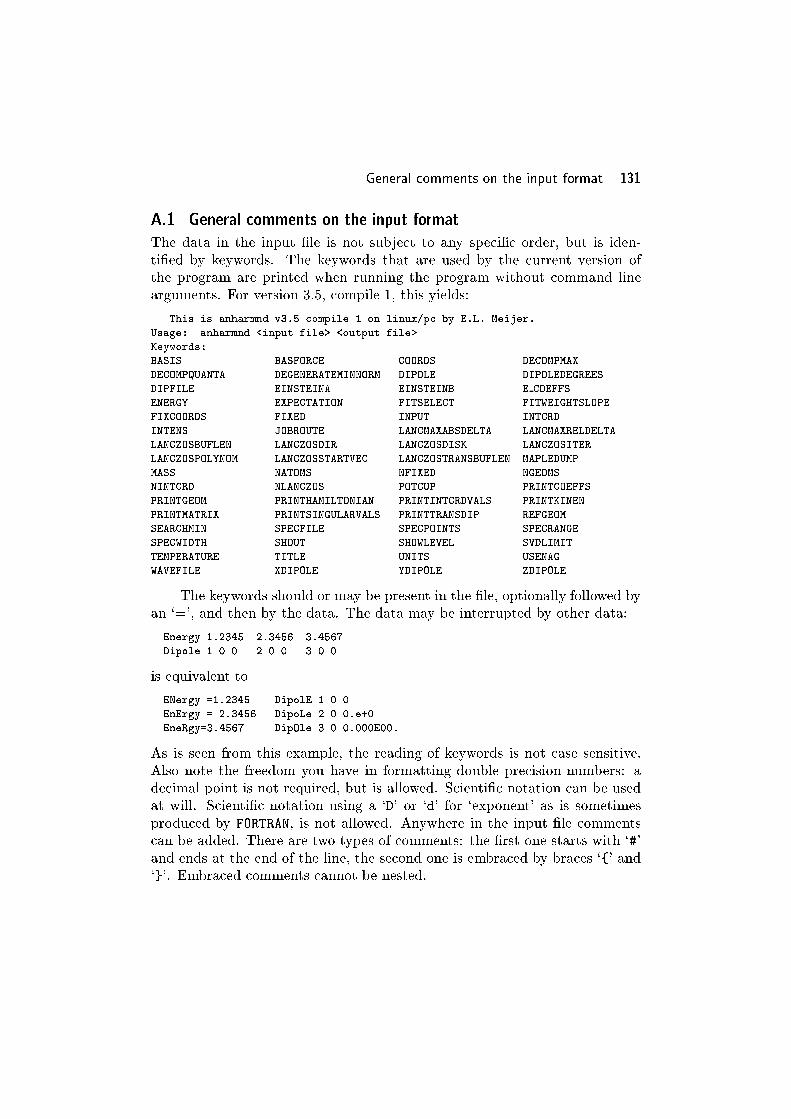
General comments on the input format 131
A.1 General comments on the input format
The data in the input �le is not subject to any speci�c order, but is iden-
ti�ed by keywords. The keywords that are used by the current version of
the program are printed when running the program without command line
arguments. For version 3.5, compile 1, this yields:
This is anharmnd v3.5 compile 1 on linux/pc by E.L. Meijer.
Usage: anharmnd <input file> <output file>
Keywords:
BASIS BASFORCE COORDS DECOMPMAX
DECOMPQUANTA DEGENERATEMINNORM DIPOLE DIPOLEDEGREES
DIPFILE EINSTEINA EINSTEINB E COEFFS
ENERGY EXPECTATION FITSELECT FITWEIGHTSLOPE
FIXCOORDS FIXED INPUT INTCRD
INTENS JOBROUTE LANCMAXABSDELTA LANCMAXRELDELTA
LANCZOSBUFLEN LANCZOSDIR LANCZOSDISK LANCZOSITER
LANCZOSPOLYNOM LANCZOSSTARTVEC LANCZOSTRANSBUFLEN MAPLEDUMP
MASS NATOMS NFIXED NGEOMS
NINTCRD NLANCZOS POTCUP PRINTCOEFFS
PRINTGEOM PRINTHAMILTONIAN PRINTINTCRDVALS PRINTKINEN
PRINTMATRIX PRINTSINGULARVALS PRINTTRANSDIP REFGEOM
SEARCHMIN SPECFILE SPECPOINTS SPECRANGE
SPECWIDTH SHOUT SHOWLEVEL SVDLIMIT
TEMPERATURE TITLE UNITS USENAG
WAVEFILE XDIPOLE YDIPOLE ZDIPOLE
The keywords should or may be present in the �le, optionally followed by
an `=', and then by the data. The data may be interrupted by other data:
Energy 1.2345 2.3456 3.4567
Dipole 1 0 0 2 0 0 3 0 0
is equivalent to
ENergy =1.2345 DipolE 1 0 0
EnErgy = 2.3456 DipoLe 2 0 0.e+0
EneRgy=3.4567 DipOle 3 0 0.000E00.
As is seen from this example, the reading of keywords is not case sensitive.
Also note the freedom you have in formatting double precision numbers: a
decimal point is not required, but is allowed. Scienti�c notation can be used
at will. Scienti�c notation using a `D' or `d' for `exponent' as is sometimes
produced by FORTRAN, is not allowed. Anywhere in the input �le comments
can be added. There are two types of comments: the �rst one starts with `#'
and ends at the end of the line, the second one is embraced by braces `{' and
`}'. Embraced comments cannot be nested.

132 Appendix A: AnharmND User's Manual
A.2 Basic keywords and data items
The following shows a fragment of an input �le with some basic keywords and
their explanations.
NAtoms = 6 # sets the number of atoms
NIntCrd = 3 # the number of internal coordinates
basis = 6 6 6 {the highest order Hermite function that is used in the
basis functions for each internal coordinate}
mass
4.918358e+04
2.915649e+04
2.915649e+04
5.099804e+04
1.837133e+03
2.552564e+04 # masses of the atoms
units angstrom # distances and positions that follow are in Angstrom
RefGeom
1.752689 -1.034773 0
-0.028374 -0.34543 0
-0.028374 -0.34543 0
-1.60085 -0.834865 0
0.090691 0.664601 0 # Specifies x, y, and z coordinates for each atom
-0.028374 2.355531 0 # in the reference geometry
NFixed = 3 # three atoms will be fixed
fixed 2 4 5 # numbers of the atoms that will be fixed
ShowLevel 20 # ask for computation of the first 20 vibrational levels
# (default is 8 levels)
title {This is the job title. It is possible to have a "title" of more
than one line, so you can add long comments to your job input, which will
also be printed in the output file.}
The title keyword di�ers from all the others in that it takes an `em-
braced comment' as an argument. If there are any �xed atoms, the reference
geometry de�nes their position, otherwise it de�nes the reference for applica-
tion of the Eckart conditions on input geometries. Furthermore the reference
geometry is used for the de�nition of internal coordinates in terms of stretches
and bendings, as described in the following section. Most of the time you will
want to use the geometry of minimal energy as `RefGeom'.

Internal coordinate speci�cation 133
A.3 Internal coordinate speci�cation
The IntCrd keyword is used for the speci�cation of internal coordinates.
There are �ve basic types of coordinate:
stretch : a stretch coordinate
shrink : a stretch in the opposite direction than stretch
bend : a bending in a speci�ed plane
pbend : a bending perpendicular to a speci�ed plane
gencoord : a movement speci�ed in atomic displacements
The shrink coordinate is useful to de�ne combined asymmetric stretches. The
gencoord coordinate is speci�ed by the displacement in cartesian coordinates
with respect to the refgeom geometry, of all atoms that were not declared as
fixed. The coordinates AnharmND uses consist of a linear movement of one
or more atoms. A coordinate speci�cation has the following format:*
IntCrd <coord> degree <d>;
where <coord> = <simple coord> [combine <coord>]:
A <simple coord> can be combined via the combine keyword with an arbitrary
number of others. The speci�cation of a coordinate is terminated by the
maximum power <d> it may get in the polynomial expansions for the energy
and the dipole surface. The <simple coord> has three possible forms:
<simple coord> =8<:(stretch|shrink) <r1 r2> [friend <f1 : : : fn> 0]
(bend|pbend) <r1 r2> plane <p1 p2 p3> [friend <f1 : : : fn> 0]
gencoord <x1 y1 z1> : : : <xn yn zn>
9=;
In this expression r1 and r2 are numbers of the `reference atoms', that de�ne
the `bond' (not necessarily a chemical bond) relative to which the stretch and
bending coordinates are de�ned. The atom denoted by r1 is the atom that
will move in this coordinate. If there are more atoms that should move along
with r1, they can be speci�ed behind the friend keyword. In the case of the
bending coordinates it is necessary to specify a plane through three atoms with
numbers p1, p2, and p3 in which (bend), or perpendicular to which (pbend) the
atom r1, and optionally f1 : : : fn should move. Note that a series of `friends'
should be terminated with a zero. In the case of a gencoord the displacements
in x, y and z direction of all the atoms that are not �xed are listed.
* `<meta expression>': not literal; `[optional]': not required;
`keyword': literal; `(one|two)': one of two possibilities.

134 Appendix A: AnharmND User's Manual
The following example shows part of what could be the input for a cal-
culation on H2O:
units AMU Angstrom
NAtoms=3 NIntCrd=3 MASS 15.99491 1.00783 1.00783
RefGeom 0.0000 0.0000 0.1135 # atom nr.1: O
0.0000 0.7530 -0.4541 # atom nr.2: H
0.0000 -0.7530 -0.4541 # atom nr.3: H
IntCrd
# symmetric stretch:
stretch 2 1 combine
stretch 3 1 degree 4
# asymmetric stretch:
stretch 2 1 combine
shrink 3 1 degree 4
# bending:
bend 2 1 plane 1 2 3 combine
bend 3 1 plane 1 3 2 degree 4
The `units' keyword (vide infra) is used to indicate that the masses are
in atomic mass units and the reference geometry is in �Angstroms instead of
atomic units. Especially note the order of the `plane' atoms in the bending
coordinate. The direction of the movement of the atoms is computed as the
outer product of the bond direction (indicated by the reference atoms) and
the normal of the plane. This implies that if you put the plane atoms in the
same order for the second <simple coord> bending as for the �rst, the H-atoms
would be moving simultaneously to the left or the right relative to the O-atom,
instead of the desired motion where the �v mirror plane perpendicular to the
H{O{H plane is conserved. To demonstrate the use of `friend', another
de�nition (somewhat cumbersome) of a symmetric bending is given:
stretch 1 2 friend 3 0 combine
stretch 1 3 friend 2 0 degree 4
This bending would, after correction for conservation of centre of mass
and angular momentum, be equal to the previous one only if the H{O{H angle
was 90Æ.

Input of energy and dipole surfaces 135
A.4 Units in the input �le
The `units' keyword controls the units that the program assumes to be used
in the input �le. The following units are currently available:
units Angstrom # length in Angstrom
Debye # dipoles in Debye
kJoule # energy in kJoule/mol
kCal # energy in kCal/mol
eV # energy in electron-volt
cm # energy in 1/cm
AMU # masses in atomic mass units
If you specify more than one energy unit, the last one will be used. Without
`units', the program assumes atomic units. Speci�ed units apply to all data
following the `units' statement, until another speci�cation is encountered.
This means that you can have a reference geometry in �Angstrom and coordi-
nates in Bohr using two units speci�cations. The default setting of atomic
units can be regained by
units reset # from this point on a.u. assumed until next `units'
A.5 Input of energy and dipole surfaces
A.5.1 Input as a series of `points'
In this case you provide a number of molecular geometries with corresponding
energies and (optional) dipole components. NGeoms: number of geometries;
energy: energies corresponding with the molecular geometries; coords: x, y,
and z coordinates of the atoms; and dipole: x, y, and z-component of the
dipole vector. A part of the input �le for H2O might be:
NGeoms = 10
units reset Angstrom Debye
# H2O011.out 1
COORDS 0.000000 0.113401 0.000000
0.752243 -0.451941 0.000000
-0.752243 -0.455264 0.000000
Energy -76.0236102222
Dipole 0.0015 -2.1464 0.0000
# and so on for the other 9 geometries....
In case the dipole is not available for all points, a missing dipole should be
indicated by dipole none, so that dipoles are associated with the right ge-
ometry. If the number of dipoles is substantially smaller than the number of
energies, the dipole should be �tted with a lower degree polynomial than the
energy, this can be done with the DIPOLEDEGREES keyword. The energy poly-
nomial degrees are speci�ed along with the internal coordinates, as described
in section A.3.
DipoleDegrees 1 1 1 # a dipole surface linear in all three coordinates

136 Appendix A: AnharmND User's Manual
A.5.2 Input as a polynomial
If you want to input energy and dipole surface as polynomials, you need to
type
input = polynom # as opposed to `input = geom', which is default.
Then you specify the polynomials representing energy as follows:
units reset # atomic units in this case ...
energy
0 0 0 -7.602361502033e+01
0 0 1 8.039523818762e-09
0 0 2 2.955394356411e-02
0 1 0 -8.671613638301e-09
0 1 1 9.567846150664e-11
0 2 0 1.700509483926e-01
1 0 0 -3.236071470050e-08
1 0 1 1.792776354046e-02
1 1 0 -3.348405953490e-10
2 0 0 1.590572688729e-01
In this format the integers identify the coeÆcient: if the coordinates were q1,
q2, and q3, then 1 3 2 would mean the coeÆcient of the q1q32q
23 term. The
coeÆcients have to apply to the internal coordinates speci�ed in the input
�le. Usually, they will be produced by the program itself. The di�erent
components of the dipole are input in the same way using XDipole, YDipole,
and ZDipole. AnharmND normalizes any coordinate it reads in such a way
thatP
i
px2i + y
2i + z
2i = 1, where xi, yi, and zi are the displacements of atom
i in the three spatial directions. The program then assumes that the energy
and dipole polynomials are de�ned in terms of these normalized coordinates.
The length units assumed for the coordinates are those given before the energy
speci�cation.
A.5.3 Combined input
It is possible to specify a polynomial for energy and dipole, and extra geome-
tries with energies and dipoles to �t extra coeÆcients. This could be used
to take the result of a force constant calculation from an electronic struc-
ture program, and compute anharmonic coeÆcients from extra points. In the
input �le input = geom polynom should be speci�ed. The geometries with
energy and dipole should be speci�ed in the same way as with input = geom,
and the polynomial coeÆcients should be speci�ed in the same way as with
input = polynom, except that the keyword for the energy polynomial now
becomes e coeffs, to distinguish it from the energies belonging to the ge-
ometries.

Di�erent job routes, restarting jobs, writing data to disk 137
A.6 Computation of properties
Computation of expectation values of coordinates and squares of coordinates
is requested by expectation = yes.
Computation of infrared absorption intensities can be done only if the
dipole surface is provided in some way or another, and should be requested by
intens = yes. By default the program only computes absorption intensities
relative to the population of the lowest level. The transitions from the ground
level to an excited level then represent the infrared spectrum at 0K. Intensities
at a given temperature are computed if temperature = <some value> is spec-
i�ed in Kelvin. Computation of Einstein A and B coeÆcients, for spontaneous
and stimulated emission respectively, can be requested with EinsteinA = yes
and EinsteinB = yes.
A.7 Di�erent job routes, restarting jobs, writing data to disk
The wave functions and transition dipoles computed by the program can be
written to disk in binary format. This allows for the computation of properties
in a second job, or computing infrared absorption intensities without having
to redo the entire quantum mechanical calculation. Currently, there are four
job routes implemented, speci�ed by the JobRoute keyword:
JobRoute = CompleteJob {does not read any data from disk}
JobRoute = IntensOnly {starts computation after reading wave functions}
JobRoute = ExpectOnly {reads wave functions,
computes expectation values from them}
JobRoute = PropOnly {reads wave functions and transition dipoles
to compute properties}
Wave function data is written to and read from a �le speci�ed by the keyword
WaveFile. The �le used for the transition dipoles is speci�ed by DipFile.
Whether the data is being written or read is determined by the JobRoute
keyword, e.g. in
JobRoute = IntensOnly
WaveFile = myjob.wave
DipFile = myjob.dip
MapleDump = myjob.map
the �le myjob.wave is read, and myjob.dip is written. AnharmND will write
the potential energy surface to a �le that is readable by the MAPLE program
if MapleDump = <�le name> is speci�ed.

138 Appendix A: AnharmND User's Manual
A.8 Using a `potential energy cup'
It is possible that the polynomial used to describe the potential energy ap-
proaches to �1 in a certain direction. If the basis functions then penetrate
into the area where the energy polynomial has large negative values, un-
physical `vibrational levels' will be found with low (negative) energies. This
situation is recognized by the fact that, if the basis set is enlarged, new lev-
els are computed that are lower in energy than the ground level in previous
calculations. Also, if the problem occurs, the ground level wave function will
contain basis functions with high quantum numbers as major components.
The program provides a solution to this problem in the form of the `poten-
tial energy cup'. A polynomial of high, even order is included in the potential
energy, providing `walls' at large distances from the minimum in the potential
energy. There are two ways to specify a potential cup:
PotCup = 8 6 10 coeff 3e-10 2e-11 1e-12 # (1)
PotCup = 8 6 10 height 0.01 0.01 0.01 # (2)
If the internal coordinates are q1, q2, and q3, (1) describes a potential
cup function
(3 � 10�10) q81 + (2 � 10�11) q62 + (1 � 10�12) q103 :
In de�nition (2) the height of the potential energy cup is speci�ed at the bor-
ders of the sampled area of the potential energy surface. The PotCup keyword
assumes atomic units always. It cannot be used with input = polynom.
If a potential cup is used, the program �rst �ts the potential in the same
way it would do otherwise, and then shifts the origin to the minimum. Then it
subtracts the value of the potential energy cup from the input energy points,
and �ts the potential energy again. The polynomial �tted to this corrected
surface is added to the potential energy cup function to yield the potential
energy that will be used in the Hamiltonian. From this it will be clear that
it makes no sense to specify a potential cup of an order not higher than the
maximum order of the polynomial that �ts the potential energy. Note that it
is possible to give one or more coeÆcients of the potential cup a value of 0.
The program will print average values of the correction applied to the
input energies, in order to provide an idea of how big its in uence will be.
Also it computes the expectation values of the `cupless' Hamiltonian of the
wave functions, so they can be compared with the eigenvalues. In the ideal
case there should be very little di�erence. The higher the order of the potential
energy cup, the atter it will be near the origin, and steeper further away. It
seems therefore best to make this order very high. However, you pay for this in
computation time, since the number of non-zero elements in the Hamiltonian
will grow.

Adjusting computational parameters 139
Warning: I have not used the PotCup feature a lot. It is possible that it
does not operate well with some of the input possibilities. Be sure to check
if the output is reasonable.
A.9 Adjusting computational parameters
A.9.1 Control of the �t procedure
The keyword FitSelect controls the way the �ts of energy and dipole surface
are done. It has three possible options. The default value is order, which
implies the program will use coeÆcients up to the order speci�ed by the user
in the internal coordinate speci�cation. If orders of the internal coordinates
are not all equal, the program chooses the coeÆcients in such a way that
a `weighted total order' does not exceed the speci�ed orders. If the option
FitSelect = automatic is speci�ed, AnharmND will try to �nd a number
of coeÆcients as close as possible to the number of input points. The option
FitSelect = user allows the user to specify explicitly which coeÆcients to
use. First the number of coeÆcients should be given, then the powers of the
coordinates of the terms that should be included in the �t. For H2O this could
be:
FitSelect = user
4 # going to use only 4 coefficients
0 0 0
2 0 0
0 2 0
0 0 2
With internal coordinates fqig this would specify a potential energy of the
form
c000 + c200 q21 + c020 q
22 + c002 q
23 :
If the constant term is not speci�ed by the user, it will be included by the
program.
The �ts of energy and dipole surfaces are done by a least squares �t.
For each point in the input a linear equation in the polynomial coeÆcients
is set up. This yields a set of equations Ax = b, where x are the values of
the energy or dipole component, the rows of A the corresponding products
of internal coordinates, and x the polynomial coeÆcients. A singular value
decomposition (SVD) of A is then performed, yielding A = UT�V. � is a
diagonal matrix which is uniquely de�ned under the condition that its values
are non-negative and non-increasing down the diagonal. If this is so, its values
f�ig are called singular values. For least squares problems like this one, the
condition number of the matrix is given by �1=�n, if A is m� n and m � n.
AnharmND prints the singular values if you put PrintSingularVals=yes
in your input �le. For each equation there is an associated singular value

140 Appendix A: AnharmND User's Manual
indicating how `important' it is. A relatively small singular value relates to
an equation that does not change the quality of the �t very much, but does
change the values of the �tted coeÆcients. Before computing the values of the
coeÆcients from the decomposed A, the program sets �i for which �i=�0 < �
to 0. This implies that the associated equations will not in uence the values
of x. Using the option SvdLimit = <some value> the limit for setting �i to
0 is changed. The default value is � = 1 � 10�6.The �ts can be weighted. The weight factors attributed to the input
points are computed according to wi = Ne�f �Ei . N is a normalization factor,
f is a factor provided by the user with FitWeightSlope = <some value>, and
Ei is the energy of input geometry i.
A.9.2 Control of the Lanczos procedure
The Lanczos procedure is an iterative way to solve eigenvalue problems. If
more iterations are done, more levels are found with greater accuracy. The
number of iterations can be set by the keyword LanczosIter. The default
value is 200, which is enough for some small problems, but certainly not for
larger ones. A `raw' Lanczos method produces `spurious eigenvalues', which
are not really eigenvalues, but an artifact of the method. Also, eigenvalues
are found with very poor accuracy, and they may be found more than once.
The program has several ways of �ltering these values out. The most impor-
tant way of �ltering out spurious eigenvalues is computing the deviation of
the expectation value of the corresponding eigenvector:phE2i � hEi2. If the
eigenvector is exact, it should have a deviation of 0. The program has two pa-
rameters to decide whether the eigenvalue is accurate enough (`sharp enough')
or not: LancMaxAbsDelta and LancMaxRelDelta. If the absolute value of the
eigenvalue is smaller than LancMaxAbsDelta, twice the deviation (i.e., the
width) divided by the absolute value of the eigenvalue should not exceed
LancMaxRelDelta. In the other cases twice the deviation should not exceed
LancMaxAbsDelta. Default values are:
LancMaxAbsDelta = 1.0e-5
LancMaxrelDelta = 1.0e-3
These keywords assume atomic units always. If a system has degenerate levels,
the program tries to �nd a complete set of orthogonal wave functions for each
degenerate level, but no more. If the program �nds two eigenfunctions that
have the same eigenvalue within the limits of LancMaxAbsDelta, it computes
the overlap between the two normalized vectors. If this overlap is smaller
than 1�DegenerateMinNorm, a Schmit-orthogonalization is done, which thenyields two orthogonal vectors. If more wave functions are found with the same
eigenvalue, it is attempted to construct a larger orthogonal set. By default
we have DegenerateMinNorm = 0.02.

Adjusting computational parameters 141
If the memory usage of the program becomes too large, the vectors pro-
duced by the Lanczos method can be written to disk. The following options
apply:
LanczosDisk = yes # as opposed to default `no'
LanczosDir = /TMP # directory for putting temporary file
LanczosBufLen = 100 # default value
LanczosTransBufLen = 100 # default value
The �les AnharmND creates for temporary storage of vectors are named
VecStorFile<pid> <nr>, where <pid> is the process id of the running job,
and <nr> is a number starting at 1, which will raise if more �les are used.
LanczosDir defaults to the current directory. The keywords LanczosBufLen
and LanczosTransBufLen control how many vectors are kept in core memory
during the Lanczos procedure and the transposing of the matrix on disk which
is necessary after the Lanczos procedure. Larger values for these bu�ers mean
larger memory usage, but also higher speed.
Normally the lanczos procedure will start with a random starting vector.
It is possible to choose a starting vector in the following way:
LanczosStartVec = 1 0 0 1
This results in a starting vector with equal, non-zero coeÆcients for the �rst
order Hermite function in the �rst and in the fourth coordinate, and zero
coeÆcient for all others. The idea is that the lanczos procedure is started
with a certain bias towards eigenfunctions that are similar to the starting
vector, to ensure they will be found within a reasonably small amount of
iterations. This doesn't seem to work very well in practice.
For larger problems where the eigenvalues are very closely spaced, the
Lanczos procedure doesn't always �nd the desired eigenfunctions within a
reasonable� number of iterations. AnharmND provides the method of poly-
nomial modi�cation of the eigenvalue spectrum to improve the relative spacing
of eigenvalues. If you want to �nd all eigenvalues below a certain value Em,
and the eigenvalue spectrum runs from E0 to Ee, you have to �nd a polynomial
f(E) so thatf(Em)� f(E0)
f(Ee)� f(Em)�
Em � E0
Ee �Em:
The lanczos procedure is then performed with f(H) instead of the Hamiltonian
H. The operator f(H) has the same set of eigenvectors f ig as the originalH, but the desired vectors are found more easily, because the eigenvalues are
� The program uses the eigenvectors for a considerable part of its calcula-
tions. If only eigenvalues were required, it would be feasible to do many more
iterations.

142 Appendix A: AnharmND User's Manual
not as closely as those from H. The eigenvalues of H are then computed as
h ijHj ii.The polynomial should be speci�ed in the input �le by its coeÆcients,
leaving out the constant term, which has no e�ect anyway, as follows:y
LanczosPolynom = -1 2 -3.5 end # specifies -x + 2 * x^2 - 3.5 * x^3
More than one polynomial can be used in one job. This might be useful if
you have di�erent polynomials that stress di�erent parts of the eigenvalue
spectrum. The syntax is as follows:
NLanczos = 2 # ask for two lanczos procedures
LanczosPolynom -1 2 3.5 end # first polynomial
LanczosPolynom 1 end # second `polynomial': plain lanczos
LanczosIter 400 500 # iteration counts for different polynomials
The results of the two Lanczos procedures will be merged, and the best con-
verged levels of lowest energy will be taken from them.
A.9.3 Adjusting minimum search and basis set
The basis functions used are products of Hermite functions of the internal co-
ordinates. In the standard procedure the program attempts to �nd a minimum
in the potential energy, then computes the second derivative of the energy with
respect to the internal coordinates, and uses this information, combined with
the `reduced mass' of the coordinate, to compute the pre-exponential factor
of the Hermite functions.
There are several situations where this will not work properly. It may
happen that the minimum in the potential energy only is a local minimum,
and you have to use a potential cup (vide supra). In that case it may be
e�ective to reduce the initial step size used in the simplex procedure that
searches for the minimum. This can be done by
SearchMin = 0.2 # reduces the initial simplex step size by a factor of 5
Usually, the reference geometry (RefGeom) will be the geometry of lowest
energy. If you know this is true, the search for the minimum can be omitted
entirely by SearchMin = 0.
Another case where searching a minimum is not what you want is a
double well potential. The Reference geometry then typically represents a
saddle point on the energy surface. It is possible to �x certain coordinates
during the minimization using the FixCoords keyword. If the curvature in
the origin of the �xed coordinate is negative, you have to provide the force
y The `polyno2' program is available to create a polynomial that stresses
the beginning of the eigenspectrum.

Plotting and Decomposing Spectra 143
constant to be used for the basis function yourself with the BasForce keyword.
For a 4-dimensional problem, this may look like this:
FixCoords 0 0 1 0 # keep 3rd coordinate fixed
BasForce 0 0 0.02 0 # only the 3rd force constant provided by the user
The program here derives the force constants for the 1st, 2nd, and 4th internal
coordinate in its usual way from the potential energy polynomial. Of course
BasForce can be used to change the pre-exponential factors of basis functions
for other reasons as well, though in general the choice of the program is a
good one. This keyword again assumes atomic units.
A.9.4 Using NAG library for matrix diagonalisation
AnharmND does not contain any NAG library functions. It can use the
separate program `trieig nag' to use the NAG library function for diagonali-
sation of the tridiagonal matrix which is part of the Lanczos procedure. For
larger problems (several thousands of Lanczos iterations) this can yield a
considerable speedup of the calculation. It is requested in the input �le by
UseNag = yes. AnharmND communicates with trieig nag using a temporary
�le named `anharmnd<pid>.tmp', where <pid> is the process id number. The
program fails if trieig nag is not found. The CPU time usage as reported by
AnharmND does not include the time the trieig nag program uses. This gives
a misleading idea as to how much faster it is.
A.10 Plotting and Decomposing Spectra
If the temperature keyword is used, it is possible to obtain a data �le that
can be used to plot an infrared spectrum with a program like gnuplot.
SpecFile = job.spec # the file name for the plot data
Specrange = 0 4000 # the range in 1/cm where peaks should be plotted
SpecWidth = 10 # halfwidth of the gaussians that represent peaks
SpecPoints = 1000 # by default, 1000 points are used for the spectrum
Note that the SpecRange is always speci�ed in cm�1, the default range is
0{4000. Each peak in the infrared spectrum is convoluted with a normalized
gaussian of the width indicated by SpecWidth (also in cm�1, default 10). As
a result the plotted peaks in the spectrum will have the correct surface area,
whereas the peak width will be arbitrary.
The program o�ers the possibility to make a decomposition of the infrared
spectrum with respect to the used vibrational coordinates. The procedure it
uses is diÆcult to describe in detail here, but the general idea is the following.
To compute the `partial excitation spectrum' of the �rst coordinate, the pro-
gram takes the �nal state of each transition, and projects this onto a space
of states that were constructed as excitations or de-excitations of the initial
state, all of which were at least excited in the �rst coordinate. The square
144 Appendix A: AnharmND User's Manual
of the norm of this projection is used as a factor by which the intensity of
the transition is multiplied to yield the partial spectrum. This is done for
de-excitations too, and for all coordinates.
These partial spectra are written into the SpecFile starting from the
third column, after the x and y data of the full infrared spectrum: �rst the
excitation spectrum of the �rst coordinate, then the de-excitation spectrum of
the �rst coordinate plotted in the negative direction, then the partial spectra
for the other coordinates. There are two keywords that control this calcula-
tion.
DecompQuanta = 3 # the number of excitation quanta used
DecompMax 2 2 2 # the maximum number of quanta used per coordinate
If you specify a lot of excitation quanta, the calculation may take a very long
time. The resulting spectra only add up to yield the exact `total spectrum'
if the coordinates are normal coordinates and the potential energy surface
is the corresponding harmonic potential. The results are dependent on the
coordinates chosen and should be used with caution.
A.11 Print Switches
PrintCoeffs = <n> requests the printing of the n largest coeÆcients of the
basis functions in the wave functions.
The following keywords should all get the value yes or no. PrintGeom
prints rotated and translated input geometries, in atomic units. The printing
of the Hamiltonian in second quantization representation can be requested
with PrintHamiltonian. PrintIntCrdVals prints the values of the inter-
nal coordinates for each input geometry. PrintKinEn prints the inverse mass
matrix. PrintMatrix requests the printing of non-zero elements of the Hamil-
tonian. This easily results in huge amounts of printed data! So be
careful with large basis sets. PrintSingularVals prints the singular values of
SVD (vide supra). PrintTransDip prints the transition dipoles for ShowLevel
levels. The keyword shout makes the program write to the �le anharmnd.log
when it passes certain points in the source code. This is mainly for debugging
purposes and probably not of much use to the user.

BComputing Infrared Spectra with AnharmND
A Strategy
Setting up a complete series of calculations to compute the potential energy
surface, dipole surface, and �nally the infrared spectrum with AnharmND is
not a trivial task. Many choices have to be made along the way. This section
describes the various steps involved in computing an infrared spectrum with
AnharmND, and pitfalls to look out for.
This appendix sometimes refers to keywords used in the input �le for
AnharmND. The keywords are in typewriter font, to distinguish them from
normal English words, and are described in greater detail in the AnharmND
user's manual.
146 Appendix B: Computing Infrared Spectra with AnharmND
B.1 Coordinates
The number of coordinates that you can take into account in the method im-
plemented in AnharmND is limited because of the computer resources that
are required. AnharmND has no hard limit to the number of coordinates built
in, but the way basis functions are enumerated in the code may break for very
large basis sets. Although I have never driven the program that far, I suspect
it will crash in an ugly fashion when that happens. It is, however, likely that
problems that occur in the construction of a potential energy surface for sys-
tems with many coordinates will prevent people from witnessing AnharmND
break because of a large basis set. The largest number of coordinates I have
used AnharmND for is seven. This proves that it is possible, but it is certainly
not easy. I think it should be quite straightforward to use it with up to �ve
coordinates, depending on the basis set used, the nature of the modes, and
the number of vibrational wave functions that are required for the infrared
spectrum.
Coordinates in AnharmND are linear displacements of atoms. They are
de�ned with respect to the reference geometry (RefGeom) speci�ed in the in-
put �le. It is a good idea to choose coordinates that are close to forming a set
of normal modes for the given potential, because then most computed vibra-
tional wave functions can be identi�ed easily as harmonic wave functions with
a relatively small modi�cation. The internal coordinate (IntCrd) speci�ca-
tion of AnharmND allows the user to de�ne `stretch' and `bending' movements
of atoms, or to specify cartesian displacement coordinates (GenCoord). The
former is mostly useful to describe the modes of a single atom or a few equiva-
lent atoms that move with respect to the rest of a molecule, while the latter is
better suited for more complicated modes, or to enter normal modes directly.
It is important to observe that AnharmND modi�es coordinates entered
in the input �le in two ways. Firstly, if there are no �xed atoms (fixed,
NFixed), the coordinates are modi�ed in such a way that the center of mass
of the molecule is conserved (removing translational motion from the coor-
dinate), and that Eckart conditions with respect to the reference geometry
are maintained (removing rotational motion). Note that it is long ago that
I used the program without �xed atoms, so check the result carefully if you
do. Secondly, AnharmND normalizes the coordinate so that the sum of the
displacements of all the atoms in the coordinate equals 1 Bohr. This is impor-
tant to observe if a potential energy or dipole surface obtained from another
program than AnharmND is used in the input to AnharmND. AnharmND
prints the coordinates it actually uses in the output �le, and it is a good idea
to check how they relate to the reference geometry that is printed as well.
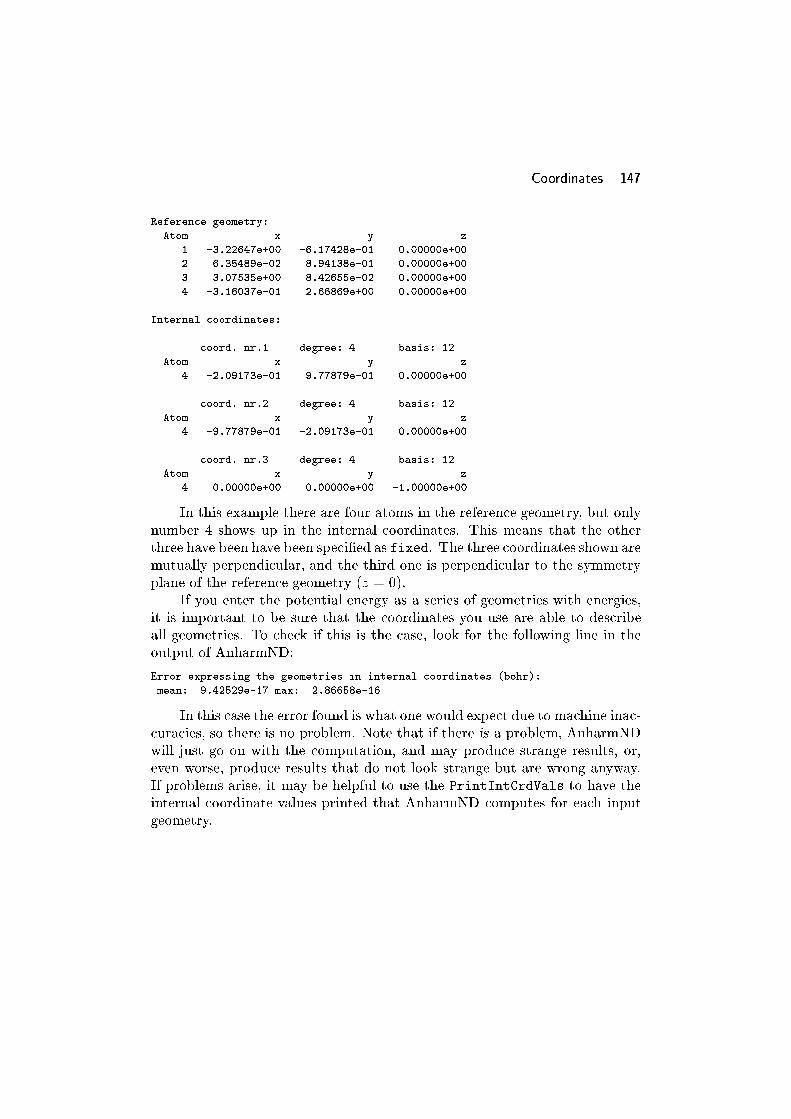
Coordinates 147
Reference geometry:
Atom x y z
1 -3.22647e+00 -6.17428e-01 0.00000e+00
2 6.35489e-02 8.94138e-01 0.00000e+00
3 3.07535e+00 8.42655e-02 0.00000e+00
4 -3.16037e-01 2.66869e+00 0.00000e+00
Internal coordinates:
coord. nr.1 degree: 4 basis: 12
Atom x y z
4 -2.09173e-01 9.77879e-01 0.00000e+00
coord. nr.2 degree: 4 basis: 12
Atom x y z
4 -9.77879e-01 -2.09173e-01 0.00000e+00
coord. nr.3 degree: 4 basis: 12
Atom x y z
4 0.00000e+00 0.00000e+00 -1.00000e+00
In this example there are four atoms in the reference geometry, but only
number 4 shows up in the internal coordinates. This means that the other
three have been have been speci�ed as fixed. The three coordinates shown are
mutually perpendicular, and the third one is perpendicular to the symmetry
plane of the reference geometry (z = 0).
If you enter the potential energy as a series of geometries with energies,
it is important to be sure that the coordinates you use are able to describe
all geometries. To check if this is the case, look for the following line in the
output of AnharmND:
Error expressing the geometries in internal coordinates (bohr):
mean: 9.42529e-17 max: 2.86658e-16
In this case the error found is what one would expect due to machine inac-
curacies, so there is no problem. Note that if there is a problem, AnharmND
will just go on with the computation, and may produce strange results, or,
even worse, produce results that do not look strange but are wrong anyway.
If problems arise, it may be helpful to use the PrintIntCrdVals to have the
internal coordinate values printed that AnharmND computes for each input
geometry.

148 Appendix B: Computing Infrared Spectra with AnharmND
B.2 Fitting a Potential Energy Surface, Basis Sets
The biggest problem for any calculation of vibrational spectra is obtaining a
proper potential energy surface. This task grows more daunting as the num-
ber of coordinates rises. The quality of the potential energy surface is the
most important limiting factor that determines the quality of the calculated
spectrum. Often the potential energy is �tted to data obtained from ab initio
electronic structure calculations. The choice of electronic structure method
is the result of considering quality versus computational cost. This is not the
place to discuss the merits of various electronic structure methods, but one
needs to realize that Hartree-Fock overestimates force constants systemati-
cally, and both Hartree-Fock and density functional theory do not describe
van der Waals interactions very well.
AnharmND uses a polynomial to represent the potential energy sur-
face. The potential energy surface can be input directly in polynomial form
(input = polynom), if you already have it. If not, this section aims to describe
how to �t one with AnharmND.
The potential energy should be well described for the range of the coor-
dinates where the computed vibrational wave functions have a non-negligible
amplitude. The problem is that you need to have a potential energy surface to
compute those wave functions to see where their amplitude is non-negligible.
This means that to get started, a �rst guess needs to be made. The �rst guess
usually is a harmonic approximation of the potential. This can be a complete
normal mode analysis with a standard electronic structure program, or the di-
agonal force constants of the coordinates involved can be computed from three
points of the potential energy around the minimum in each coordinate. The
diagonal force constant � and the reduced mass � of a coordinate q are related
to the root-mean-square displacement of the coordinate in a one-dimensional
harmonic vibrational wave function j�ii:
�(�i) �ph�ijq2j�ii =
s(i+ 1
2)�h
p��
: (1)
In this expression i is the vibrational quantum number, and �h is Planck's
constant. From the expression it is clear that higher excited states have larger
widths. If you have the wave number ~� of the transition from the ground state
to the �rst excited state of a mode, the force constant can be expressed in
terms of the wave number and reduced mass, so that you have
�(�i) =
s(i+ 1
2)�h
2�~�c�; (2)
where c is the speed of light.

Fitting a Potential Energy Surface, Basis Sets 149
The vibrational basis set used by AnharmND consists of products of one-
dimensional harmonic vibrational wave functions. By default the associated
force constants of the one-dimensional functions are taken from the supplied
potential energy surface, so their width is approximately equal to the �rst
guess computed in Eqs. 1 or 2 (the used force constant can be changed through
the BasForce keyword). The width of the highest order basis function used
poses a limit to the maximum width the computed anharmonic wave functions
can get.
In general the construction of a coordinate grid for the computation of the
potential energy surface starts from the minimum energy point. Then in the
direction of each coordinate more points are computed, and as a rule of thumb,
�(�i) for the highest order i, multiplied by a factor between 1.5 and 3, gives
the distance between minimum energy value of the coordinate and the smallest
or largest value. A highest order of 12 to 16 for one-dimensional basis functions
is a good working value to use when constructing a grid. What proves to be a
good basis set of course depends on the system and on how many excited levels
you want to compute, but these values are typical. If you do an AnharmND
computation which includes �tting the potential energy surface, AnharmND
prints some information on the width of the basis functions compared to the
points entered for the potential energy surface, as shown below.
Basis set / potential energy surface analysis.
w = sqrt(< phi | x^2 | phi >) for the highest order hermite function
min = minimum value of the coordinate in the input
max = maximum value of the coordinate in the input
(all values in atomic units)
coord. min max w min/w max/w
1 -1.100093e+00 7.146051e-01 6.300201e-01 -1.746124e+00 1.134258e+00
2 -2.193764e+00 2.206640e+00 1.222203e+00 -1.794927e+00 1.805462e+00
3 -2.200177e+00 2.200231e+00 1.867004e+00 -1.178453e+00 1.178482e+00
In this example one can see in the fourth and �fth column that the �rst
coordinate varies between �1:746124 � �(�i) and 1:134258 � �(�i). In the
AnharmND output the coordinates have a value of 0 if they correspond to the
reference geometry. If the absolute value of the numbers in the fourth and
�fth column become signi�cantly smaller than 1, this may indicate a problem
with the potential energy or with the basis set.
Note that in the example just shown, the grid is not symmetric with
respect to the �rst coordinate. This is because it is a bond stretch coordinate,
which means that for bond lengths shorter than equilibrium (in this case,
positive values of the coordinate) the energy rises more quickly than for bond
lengths longer than equilibrium. It is not necessary to sample the potential
energy for very short bond lengths because the energy becomes so high that
vibrational wave functions will not get a signi�cant amplitude in that area.

150 Appendix B: Computing Infrared Spectra with AnharmND
In general it is more important to have many points near the minimum of the
potential energy than at higher values. As a result if there are �ve points of
the grid along one coordinate, three of them will be relatively close to each
other near the energy minimum, leaving a somewhat larger gap to the extreme
points. For an atomic bend coordinate this could result in values like 0.65,
0.9, 1.0, 1.1, and 1.35, and for a stretch coordinate you could get something
like 0.8, 0.9, 1.0, 1.1, and 1.3, taking into account the asymmetry between
shorter and longer bonds.
The next issue in the construction of a potential energy grid is the number
of grid points you will use. For a meaningful polynomial �t, you will need at
least as many points as there are coeÆcients in the polynomial you are going
to use, and it is not a bad idea to have some more. Note that if you already
have the force constants of the system, you can use these and �t the remaining
coeÆcients, with the option input = geom polynom.
Polynomials of odd order give problems when they are used as represen-
tations of the energy in AnharmND, because they always go to �1 in some
direction. Therefore the smallest polynomial that one can use is a fourth order
polynomial. Because the number of points that is needed to obtain a potential
energy surface, a fourth order polynomial is often also the largest one that is
practical to use for systems with three or more coordinates. The order of the
polynomial is speci�ed per coordinate in the internal coordinate speci�cation
to AnharmND (with IntCrd). AnharmND can determine the coeÆcients used
for the polynomials �tting the potential energy and dipole surfaces in three
ways (see the user's manual). It is advisable to use the default option, which
uses all coeÆcients belonging to products of powers of coordinates where the
sum of the powers does not exceed the highest order speci�ed for a single
coordinate (assuming that the highest order is the same for all coordinates).
This kind of polynomial has the nice property that it can remain invariant
under a linear transformation of the coordinates.
Once you have a potential energy on a grid, it is time to run AnharmND
and try a �rst calculation. For the same reason that odd order polynomials
are not suitable for AnharmND, the highest even order coeÆcients of one
coordinate need to be positive, so it is important to check this in the output
of AnharmND. Problems occur if the potential bends o� to negative values
within the area where the basis functions have non-negligible amplitude. The
potential then is said to `leak', and the ground level contains high order basis
functions with large coeÆcients. If this happens, the energy of the ground level
that AnharmND computes with not converge with increasing basis set, but go
down at every increment. With the option PrintCoeffs = <n> AnharmND
will print the <n> largest basis function coeÆcients of the lowest energy wave
functions, like this:

Fitting a Potential Energy Surface, Basis Sets 151
Level: 0
Eigenvalue: 1.195740033505e-02
Coefficients:
[0][0][0] 9.783698447979e-01
[0][0][2] -1.170524365467e-01
[1][0][0] -1.119123917073e-01
[1][0][2] -7.970829924068e-02
[0][2][0] -5.648981937764e-02
In this example, the ground level's main component is a product of the 0th
order basis functions of all coordinates. If there were high order coeÆcients
very important in the ground level, this would be a sign of problems with the
potential.
AnharmND uses singular value decomposition to �t the polynomial co-
eÆcients. How this works is described in the manual. To check the results of
the SVD, put PrintSingularVals = yes in the input �le. This should yield
something like the following.
Fitting the potential energy by a polynomial.
START FITSURFACE INFO
| Fitting a polynomial of 3 variables.
| Number of equations: 125
| Fitting polynomial of specified order.
| Number of coefficients used: 35.
| The points were fitted according to user supplied weights.
| Limit for singular value zeroing: 1.000000000000e-06
| Normalized singular values:
| 1 1.00e+00
| 2 7.59e-01
| 3 7.12e-01
| 4 2.13e-01
| 8 8.09e-02
# ... leaving some values out to save paper
| 31 2.56e-03
| 32 2.48e-03
| 33 2.43e-03
| 34 1.92e-03
| 35 4.98e-08
| Number of singular values zeroed: 1
| Deviation of the fit: 6.287509691945e-04
END FITSURFACE INFO
The singular values start at 1 (by de�nition), and then gradually decrease
until the last one, which is almost �ve orders of magnitude smaller than its
predecessor. This is a typical result. Sometimes more small singular values
follow below the `well-behaved' ones. To prevent the �t to be ill-conditioned,
singular values below the gap should be set to zero in the rest of the calcula-
tion. The limit below which singular values are set to zero here is 10�6. This
can be changed with SvdLimit.

152 Appendix B: Computing Infrared Spectra with AnharmND
Further note in this example that the deviation of the �t is printed. This is
the weighted root-mean-square error of the �t. If it is not more than two orders
of magnitude smaller than the range of your energy values, something should
be done about it. By default AnharmND assigns all input points a weight
of 1. Physically, points with a lower energy are more important to compute
good vibrational wave functions. AnharmND can account for this assigning
�t weights that are proportional to the negative exponent of the energy times
a scaling factor. This scaling factor can be set with FitWeightSlope. In
this thesis I have used a FitWeightSlope of 125Eh�1. Increasing this scaling
factor will decrease the weighted root-mean-square error of the �t. At the
same time, the �t will give a better description around the minimum of the
potential at the expense of the description of the area further away.
The �t of the dipole surface is less involved than that of the potential
energy surface. If x, y, and z-components of the dipole are given for all the
input geometries, each component is �tted with a polynomial of the same
shape as the potential energy. It is possible to leave out the dipole for any
number of the points using Dipole none. For the computation of the infrared
spectrum it is often enough to supply just the constant part and the �rst
derivatives of the dipole in polynomial form. If you want to use di�erent
order polynomials to �t the dipole surface with AnharmND than to �t the
potential energy, you need to run the program more than once, and take
advantage of the options of restarting the program at a di�erent stage of the
calculation.
After the �t, AnharmND tries to �nd the minimum of the potential energy
before it continues with the vibrational calculation (unless you tell it not to,
with the SearchMin or FixCoords options). When the minimum is found,
the origin of the potential energy polynomial is shifted to that minimum, and
the force constants at the minimum are used for the one-dimensional basis
functions (unless changed with BasForce). If you copy the �tted potential or
dipole surface from an AnharmND output �le to reuse it in an input �le, you
should look careful if you have the version before or after shifting the origin.
For both potential energy and dipole surface, both versions are printed.

AnharmND's Lanczos Procedure 153
B.3 AnharmND's Lanczos Procedure
The Hamiltonian is diagonalized in AnharmND using a Lanczos or a modi�ed
Lanczos method, that is described in some detail in the manual. The number
of levels that the program tries to �nd is speci�ed with ShowLevel. The
number of iterations used in a Lanczos procedure is given with LanczosIter.
It is important to check if the Lanczos procedure converged well enough for
the levels you are interested in. This can be done looking at the output where
the computed energies are printed:
Total energies:
level E(Hartree) Low limit High limit Deviation
v=0 1.19574003e-02 1.19573999e-02 1.19574008e-02 3.64e-06 %
v=1 1.44139347e-02 1.44139344e-02 1.44139351e-02 2.55e-06 %
v=2 1.71823493e-02 1.71823488e-02 1.71823498e-02 3.03e-06 %
v=3 1.72581059e-02 1.72581053e-02 1.72581065e-02 3.57e-06 %
v=4 1.99338610e-02 1.99338606e-02 1.99338614e-02 2.02e-06 %
The energies refer to the potential energy polynomial without the con-
stant term. If AnharmND shifted the origin of the polynomial to the energy
minimum, then the shifted polynomial without the constant term is the ref-
erence, and the energy of the lowest level is the zero-point vibrational energy
of the system.
In the columns `Low limit' and `High limit' the boundaries between which
it has been determined that an exact eigenvalue of the Hamiltonian is located
are printed. The `Deviation' column lists the maximum error in as a percent-
age of the vibrational energy. In this example the accuracy of the computed
levels is good. There are several options that determine what AnharmND
considers `good' enough to print in the output �le, LancMaxAbsDelta and
LancMaxAbsRelData. If the levels that AnharmND prints are not accurate
enough to your liking, you set these parameters to tighter values. If you do
not �nd enough levels, you can either set the LancMax...Delta parameters to
larger values, or raise the number of iterations. If that does not help enough,
it is possible to use a modi�ed Lanczos method with LanczosPolynom. If
there are vibrational levels with degenerate energies, AnharmND should be
able to �nd the correct number of them. If it does not seem to �nd more
than one of a set of degenerate levels, the parameter DegenerateMinNorm can
be set to a smaller value than its default of 0.02. The manual describes the
Lanczos procedure in greater detail.

154 Appendix B: Computing Infrared Spectra with AnharmND
B.4 Analysis of the Results
Besides infrared absorption intensities, also Einstein A and B coeÆcients (at
virtually no extra cost) and expectation values can be computed from the
vibrational wave functions. The expectation values of the coordinates and
squares of the coordinates give information about the width of the wave func-
tions, so that a comparison with the grid used for the potential energy becomes
possible.
In practice you will usually not compute these properties in the �rst run
of AnharmND, and if the computations take longer than a few minutes, it is a
good idea to store the wave functions and dipole moments with the WaveFile
and DipFile commands. This data can be reused in subsequent runs of the
program by setting the right JobRoute.
To analyse the results of a AnharmND calculation, one can print the
coeÆcients of the basis functions as shown earlier. If the number of wave
functions increases, it becomes harder to understand the results just by look-
ing at the table with absorption intensities. Plots of the infrared spectrum
can be made from the data AnharmND generates with the SpecFile option.
Although AnharmND does not compute peak widths, I have chosen not to
represent peaks in the spectrum plots with spikes with a height representing
the integrated absorption intensity, but with the convolution of such spikes
with gaussian curves of a �xed width with unity surface area. The reason for
this choice is that in this way the plotted absorption intensity stays correct if
peaks are very close to each other in frequency, whereas spikes would overlap
each other in the plot, without showing an appropriate increase in height.
Plotted spectra always represent the absorption intensities weighted by
a Boltzmann distribution at a certain temperature, which can be speci�ed
in the input �le with the Temperature option. If you do not specify the
temperature, AnharmND will set it to 298.15K.
AnharmND provides a way to decompose spectra into `partial spectra' for
each coordinate used, with the DecompQuanta and DecompMax options. This
may be of some value in the analysis of spectra, but one should be well aware
what they mean, and what they do not mean. The partial spectra do not
generally add up to yield the full infrared spectrum. More information about
this procedure is given in the manual, and in chapter 4 of this thesis.
Summary 155
Summary
This thesis deals with the infrared spectrum of acidic zeolites with adsorbed
acetonitrile. In this spectrum the OH stretch vibration of the acidic OH groups
at 3610 cm�1 is replaced by two broad bands with frequencies of ca. 2400 cm�1
and 2800 cm�1. In the beginning of the research project there has been a col-
laboration with J. J�anchen and J. van Wolput who measured infrared spec-
tra, and with A.G. Pelmenschikov who performed standard quantum chemical
computations using a simple cluster molecule. During this collaboration we
have discovered that the broad bands in the spectrum with acetonitrile are
due to a Fermi resonance of the OH stretch mode with an overtone of an OH
bending mode.
With standard quantum chemical program packages infrared spectra can
only be computed in the harmonic approach. This approach is not suited to
reproduce Fermi resonance. In my graduate research I have written a com-
puter program that can compute infrared spectra (frequencies and integrated
absorption intensities) including anharmonicities. The program is generally
applicable to systems with a limited number of linear coordinates. The the-
oretical background used for the program is described in Chapter 2 of this
thesis, and the Appendices A and B describe its use.
Chapters 3 and 4 describe calculations of the infrared spectrum of an
acidic zeolite with acetonitrile using potential energy and dipole surfaces ob-
tained in the so-called `cluster-approach'. In this approach the acidic site of
the zeolite is modeled with a small molecule in which the acidic OH group of
the zeolite is present with a number of neighbouring atoms. In Chapter 3 three
coordinates of the acidic proton and one coordinate describing the intermolec-
ular stretch mode of acetonitrile have been used for the calculations. It has
been found that density functional theory provides better potential energy
surfaces than the Hartree-Fock approximation, but to reproduce the Fermi
resonance in the spectrum it has been necessary to apply an extra scaling of
the potential.
In Chapter 4 calculations are described of potential energy surfaces in-
cluding the coordinates of the oxygen atom of the acidic OH group. This
yields a quantitative improvement of the computed values of the frequencies,
along with a slightly better reproduction of the Fermi resonance.
Finally in Chapter 5 an account is given of the computation of the infrared
spectrum of an acidic zeolite with adsorbed acetonitrile using a model where
the zeolite cluster is embedded in a much larger part of the zeolite. The
zeolite cluster is described with Hartree-Fock, and the zeolite environment
with molecular mechanics. The embedded potential has been calculated by
A.H. de Vries. With this model it appears possible to reproduce the Fermi
resonance that has been observed experimentally in the computed spectra.
156 Samenvatting
Samenvatting
Dit proefschrift handelt over de analyse van het infraroodspectrum van
een zure zeoliet met geabsorbeerd acetonitril. In dit spectrum is de strek-
vibratie van de zure OH-groepen bij 3610 cm�1 vervangen door twee brede
banden met frequenties van ca. 2400 cm�1 en 2800 cm�1. In het begin van
het promotie-onderzoek is samengewerkt met J. J�anchen en J. van Wolput
die infraroodspectra hebben gemeten, en met A.G. Pelmenschikov die stan-
daard kwantumchemische berekeningen aan een eenvoudig cluster-model heeft
gedaan. Tijdens deze samenwerking is ontdekt dat de brede banden in het
spectrum met acetonitril het gevolg zijn van een Fermi-resonantie van de OH-
strekvibratie met een boventoon van een OH-buigvibratie.
Met de standaard kwantumchemische programmatuur kunnen infrarood-
spectra alleen worden uitgerekend in de harmonische benadering. Hiermee
kan Fermi-resonantie niet worden gereproduceerd. Tijdens de promotie is een
computerprogramma geschreven dat infraroodspectra (frequenties en ge��nte-
greerde absorptie-intensiteiten) kan uitrekenen met inbegrip van anharmonici-
teiten. Het programma is algemeen toepasbaar op systemen met een beperkt
aantal lineaire co�ordinaten. De theoretische achtergrond van het programma
wordt beschreven in hoofdstuk 2 van dit proefschrift, en de appendices A en
B beschijven het gebruik ervan.
De hoofdstukken 3 en 4 beschrijven berekeningen van het infrarood spec-
trum van een zure zeoliet met acetonitril uitgaande van potentiaal- en dipool-
opppervlakken verkregen in de zogenaamde `cluster-benadering'. Hierin is
de zure site van de zeoliet gemodelleerd door een klein molecuul waarin de
zure OH-groep van de zeoliet aanwezig is met enkele naburige atomen. In
hoofdstuk 3 werd gerekend met drie co�ordinaten voor het zure proton en
�e�en co�ordinaat voor de intermoleculaire strekbeweging van acetonitril. Het is
gebleken dat dichtheidsfunctionaaltheorie betere potentiaal- en dipoolopper-
vlakken geeft dan de Hartree-Fock-benadering, maar om de Fermi-resonantie
te reproduceren was het nodig om een extra schaling van de potentiaal toe te
passen.
In hoofdstuk 4 zijn berekeningen beschreven aan potentiaaloppervlakken
waarin ook nog de coordinaten van het zuurstof-atoom van de zure OH-groep
zijn meegenomen. Hiermee wordt een kwantitatieve verbetering bereikt van
de berekende frequenties, samen met een bescheiden verbetering in de be-
schrijving van de Fermi-resonantie.

Samenvatting 157
Tenslotte zijn er infraroodspectra berekend waarbij het zeoliet-cluster
werd ingebed in een veel groter stuk van de zeoliet. Hierbij is het cluster
beschreven met Hartree-Fock, en de zeoliet-omgeving met moleculaire me-
chanica. De ingebedde potentiaal is berekend door A.H. de Vries. Wanneer
met dit model potentiaal- en dipool-oppervlakken worden uitgerekend, blijkt
het hieruit verkregen infraroodspectrum Fermi-resonantie die experimenteel
wordt waargenomen te reproduceren.

158 Dankwoord
Dankwoord
Graag wil ik enige mensen bedanken die op de �e�en of andere wijze hebben
bijgedragen aan het totstandkomen van dit proefschrift. Rutger van Santen
en Tonek Jansen vormden de `eerste lijn' waar het ging om het opzetten van
het project en het leveren van wetenschappelijk advies. Dank hiervoor. Een
groot talent van Rutger is ook het (welhaast tot berstens toe) laten groeien
van de vakgroep, zodat er altijd wel ergens een wetenschappelijk medewerker
of postdoc rondloopt die met dezelfde materie bezig is. Van al deze mensen
wil ik graag Jochen J�anchen, Jos van Wolput en Jan de Haan speciaal ver-
noemen die aan het begin van mijn promotie experimenteel onderzoek hebben
verricht aan de systemen waar ik aan heb gerekend, en Sasha Pelmenschikov,
die bergen cluster-berekeningen heeft verricht die ik dus niet meer hoefde te
doen. Dank. Samen met Alex de Vries heb ik de berekeningen aan de em-
bedde clusters gedaan. Aan het eind van mijn promotie leverde dit aardige
resultaten op, door onze respectievelijke `hobby horses' samen te laten rennen.
Alex, bedankt voor de samenwerking. Dan zijn er ook nog mensen die een
prominente rol speelden bij het ontstaan van mijn alter ego van systeembe-
heerder. Gertjan Visser heeft me vooral in het begin op weg geholpen met
FORTRAN programma's en unix-beginselen. Een zeer constante factor in het
unix systeembeheer op het rekencentrum was `2164' Mart Mennen (dat num-
mer vergeet ik niet meer). Mart had vrijwel altijd snel `het antwoord' op
praktische vragen, en steeds weer een gulle lach wanneer de Alliant weer
eens op zijn achterste lag. Gertjan en Mart, bedankt. Via het systeembeheer
beland ik dan bij enige collega's. Ronald Gelten en Roelant Harmsen heb-
ben enige tijd geassisteerd bij het systeembeheer in de theorie-groep. Jullie
waren �jne collega's. In het rijtje bijzondere collega's die het leven in de vak-
groep kleur gaven wil ik nog speciaal noemen Kristine de Boer (met Edwin en
Dynke in haar gevolg), en mijn laatste kamergenoot Robin Milot. Dank voor
het aangename gezelschap. Graag wil ik ook mijn ouders bedanken voor de
steun aan het eind van mijn schrijfperiode. En dan, last but not least, wil ik
mijn afstudeerbegeleiders en latere collega Erik Teunissen bedanken, die mij
het wondere pad der theoretische chemie op heeft getrokken.
Eric Meijer

Curriculum Vitae 159
Curriculum Vitae
Eric Meijer werd geboren op 1 augustus 1967 te Schiedam. Hij doorliep het
gymnasium-� op het St. Paulus Lyceum in Tilburg. In 1985 begon hij aan een
studie scheikundige technologie aan de Technische Universiteit Eindhoven, die
werd afgerond in 1991 met een afstudeeronderwerp in de theoretische chemie
bij prof.dr. R. A. van Santen. Vervolgens startte hij in de vakgroep Anorgani-
sche Chemie en Katalyse van prof. van Santen een promotie-onderzoek waarin
theoretisch-chemische berekeningen werden verricht aan infraroodspectra van
zure zeolieten met geadsorbeerd acetonitril. Hij ontwikkelde software om in-
fraroodspectra uit te rekenen, en was tevens enige tijd werkzaam als unix-
systeembeheerder in de theoriegroep. Op 15 mei 2000 trad Eric in dienst van
Philips Medical systems als software-ontwikkelaar voor MR systemen. Eric
speelt klassiek gitaar en maakt sinds het begin van de jaren 1980 deel uit van
het Tilburgs Gitaar-Ensemble.