quantum chemical studies of thermochemistry, kinetics and
TRANSCRIPT

Quantum Chemical Studies ofThermochemistry, Kinetics and
Molecular Structure.
by
Naomi Louise Haworth
A thesis submitted in fulfilment of the requirements for the
degree of Doctor of Philosophy.
School of Chemistry
University of Sydney
February, 2003

Declaration
I hereby declare that this thesis is my own work and that, to the best of my knowledge, it
contains no material previously published or written by another person nor material which has
been accepted for the award of another degree or diploma at an institute of higher education,
except where due acknowledgement is given.
Naomi Haworth

For the Glory of God

Acknowledgements
I would like to express my extreme gratitude to my supervisor, Dr George Bacskay, for the
wonderful way he has helped and guided me over the past four years. Thankyou particularly
for your kindness, understanding and patience with me in the hard times. I would also like to
thank my associate supervisor, Associate Professor John Mackie, for teaching and advising
me in the kinetics work in this thesis and for proposing the projects on fluorocarbons,
phosphorus compounds and NNH + O.
I am also grateful to the many other academics and students with whom I have shared
collaborative projects, in particular Nathan Owens, Klaas Nauta and Scott Kable (CFClBr2)
and Charles Collyer and Matt Templeton (Phaseolotoxin). Thanks also to all my coworkers
over the years (Jason, Jens, Kausala, Karina, Justin, Debbie, Adam, Keiran, Siobhan and
many more) for their help and advice and for the fun we’ve shared.
I thank my family for their love and for supporting me and believing in me throughout all my
academic career, and also my friends for their support and encouragement. Particular thanks
go to Justine for all the ways, big and small, that you’ve helped me out over the past few
months and for your patience; to Evan for trying to keep me sane; and to Geoff for helping
with the proof reading.
I would like to thank the Australian Partnership for Advanced Computing (APAC) National
Facility for access to the COMPAQ AlphaServer SC system and the Australian Centre for
Advanced Computing and Communications (ac3) for access to their SGI Origin 2400
computer system. Finally, I express my sincere gratitude to the Australian Postgraduate
Association for funding my PhD scholarship.

Abstract
This thesis is concerned with a range of chemical problems which are amenable to theoretical
investigation via the application of current methods of computational quantum chemistry.
These problems include the calculation of accurate thermochemical data, the prediction of
reaction kinetics, the study of molecular potential energy surfaces, and the investigation of
molecular structures and binding.
The heats of formation (from both atomisation energies and isodesmic schemes) of a set of
approximately 120 C1 and C2 fluorocarbons and oxidised fluorocarbons (along with C3F6 and
CF3CHFCF2) were calculated with the Gaussian-3 (G3) method (along with several
approximations thereto). These molecules are of importance in the flame chemistry of
2-H-heptafluoropropane, which has been proposed as a potential fire retardant with which to
replace chloro- and bromofluorocarbons (CFC’s and BFC’s). The calculation of the data
reported here was carried out in parallel with the modelling studies of Hynes et al.1-3 of shock
tube experiments on CF3CHFCF3 and on C3F6 with either hydrogen or oxygen atoms.
G3 calculations were also employed in conjunction with the experimental work of Owens et
al.4 to describe the pyrolysis of CFClBr2 (giving CFCl) at a radiation wavelength of 265 nm.
The theoretical prediction of the dissociation energy of the two C-Br bonds was found to be
consistent with the energy at which carbene production was first observed, thus supporting the
hypothesis that the pyrolysis releases two bromine radicals (rather than a Br2 molecule). On
the basis of this interpretation of the experiments, the heat of formation of CFClBr2 is
predicted to be 184 ± 5 kJ mol−1, in good agreement with the G3 value of 188 ± 5 kJ mol−1.
Accurate thermochemical data was computed for 18 small phosphorus containing molecules
(P2, P4, PH, PH2, PH3, P2H2, P2H4, PO, PO2, PO3, P2O, P2O2, HPO, HPOH, H2POH, H3PO,
HOPO and HOPO2), most of which are important in the reaction model introduced by
Twarowski5 for the combustion of H2 and O2 in the presence of phosphine. Twarowski
reported that the H + OH recombination reaction is catalysed by the combustion products of
PH3 and proposed two catalytic cycles, involving PO2, HOPO and HOPO2, to explain this
observation. Using our thermochemical data we computed the rate coefficients of the most

Abstract
important reactions in these cycles (using transition state and RRKM theories) and confirmed
that at 2000K both cycles have comparable rates and are significantly faster than the
uncatalysed H + OH recombination.
The heats of formation used in this work on phosphorus compounds were calculated using the
G2, G3, G3X and G3X2 methods along with the far more extensive CCSD(T)/CBS type
scheme. The latter is based on the evaluation of coupled cluster energies using the correlation
consistent triple-, quadruple- and pentuple-zeta basis sets and extrapolation to the complete
basis set (CBS) limit along with core-valence correlation corrections (with counterpoise
corrections for phosphorus atoms), scalar relativistic corrections and spin-orbit coupling
effects. The CCSD(T)/CBS results are consistent with the available experimental data and
therefore constitute a convenient set of benchmark values with which to compare the more
approximate Gaussian-n results. The G2 and G3 methods were found to be of comparable
accuracy, however both schemes consistently underestimated the benchmark atomisation
energies. The performance of G3X is significantly better, having a mean absolute deviation
(MAD) from the CBS results of 1.8 kcal mol−1, although the predicted atomisation energies
are still consistently too low. G3X2 (including counterpoise corrections to the core-valence
correlation energy for phosphorus) was found to give a slight improvement over G3X,
resulting in a MAD of 1.5 kcal mol−1. Several molecules were also identified for which the
approximations underlying the Gaussian-n methodologies appear to be unreliable; these
include molecules with multiple or strained P-P bonds.
The potential energy surface of the NNH + O system was investigated using density
functional theory (B3LYP/6-31G(2df,p)) with the aim of determining the importance of this
route in the production of NO in combustion reactions. In addition to the standard reaction
channels, namely decomposition into NO + NH, N2 + OH and H + N2O via the ONNH
intermediate, several new reaction pathways were also investigated. These include the direct
abstraction of H by O and three product channels via the intermediate ONHN, giving N2 +
OH, H + N2O and HNO + N. For each of the species corresponding to stationary points on the
B3LYP surface, valence correlated CCSD(T) calculations were performed with the
aug-cc-pVxZ (x = Q, 5) basis sets and the results extrapolated to the complete basis set limit.
Core-valence correlation corrections, scalar relativistic corrections and spin orbit effects were
also included in the resulting energetics and the subsequent calculation of thermochemical
data. Heats of formation were also calculated using the G3X method. Variational transition

Abstract
state theory was used to determine the critical points for the barrierless reactions and the
resulting B3LYP energetics were scaled to be compatible with the G3X and CCSD(T)/CBS
values. As the results of modelling studies are critically dependent on the heat of formation of
NNH, more extensive CCSD(T)/CBS calculations were performed for this molecule,
predicting the 0298f H∆ to be 60.6 ± 0.5 kcal mol−1. Rate coefficients for the overall reaction
processes were obtained by the application of multi-well RRKM theory. The thermochemical
and kinetic results thus obtained were subsequently used in conjunction with the GRIMech
3.0 reaction data set in modelling studies of combustion systems, including methane / air and
CO / H2 / air mixtures in completely stirred reactors. This study revealed that, contrary to
common belief, the NNH + O channel is a relatively minor route for the production of NO.
The structure of the inhibitor Nδ-(N′-Sulfodiaminophosphinyl)-L-ornithine, PSOrn, and the
nature of its binding to the OTCase enzyme was investigated using density functional
(B3LYP) theory. The B3LYP/6-31G(d) calculations on the model compound, PSO, revealed
that, while this molecule could be expected to exist in an amino form in the gas phase, on
complexation in the active site of the enzyme it would be expected to lose two protons to form
a dinegative imino tautomer. This species is shown to bind strongly to two H3CNHC(NH2)2+
moieties (model compounds for arginine residues), indicating that the strong binding observed
between inhibitor and enzyme is partially due to electrostatic interactions as well as extensive
hydrogen bonding (both model Arg+ residues form hydrogen bonds to two different sites on
PSO). Population analysis and hydrogen bonding studies have revealed that the
intramolecular bonding in this species consists of either single or semipolar bonds (that is, S
and P are not hypervalent) and that terminal oxygens (which, being involved in semipolar
bonds, carry negative charges) can be expected to form up to 4 hydrogen bonds with residues
in the active site.
In the course of this work several new G3 type methods were proposed, including
G3MP4(SDQ) and G3[MP2(Full)], which are less expensive approximations to G3, and
G3X2, which is an extension of G3X designed to incorporate additional electron correlation.
As noted earlier, G3X2 shows a small improvement on G3X; G3MP4(SDQ) and
G3[MP2(Full)], in turn, show good agreement with G3 results, with MAD’s of ~ 0.4 and
~ 0.5 kcal mol−1 respectively.

Abstract
1. R. G. Hynes, J. C. Mackie and A. R. Masri, J. Phys. Chem. A, 1999, 103, 5967.
2. R. G. Hynes, J. C. Mackie and A. R. Masri, J. Phys. Chem. A, 1999, 103, 54.
3. R. G. Hynes, J. C. Mackie and A. R. Masri, Proc. Combust. Inst., 2000, 28, 1557.
4. N. L. Owens, Honours Thesis, School of Chemistry, University of Sydney, 2001.
5. A. Twarowski, Combustion and Flame, 1995, 102, 41.

Publications
Parts of this work have been published or submitted for publication in the following journal
articles:
N. L. Haworth, M. H. Smith, G. B. Bacskay, J. C. Mackie
Heats of Formation of Hydrofluorocarbons Obtained by Gaussian-3 and Related Quantum
Chemical Computations.
J. Phys. Chem. A 2000, 104, 7600.
N. L. Haworth, G. B. Bacskay, J. C. Mackie
The Role of Phosphorus Dioxide in the H + OH Recombination Reaction: Ab Initio Quantum
Chemical Computation of Thermochemical and Rate Parameters.
J. Phys. Chem. A 2002, 106, 1533.
N. L. Haworth, G. B. Bacskay
The Structure of Nδ-(N′-Sulfodiaminophosphinyl)-L-ornithine and its Binding to Ornithine
Transcarbamoylase: A Quantum Chemical Study.
Molecular Simulation 2002, 28, 773.
N. L. Haworth, G. B. Bacskay
Determination of Accurate Quantum Chemical Energies and Heats of Formation for
Phosphorus Compounds.
J. Chem. Phys. 2002, 117, 11175.
N. L. Owens, B. K. Nauta, S. H. Kable, N. L. Haworth, G. B. Bacskay
An Experimental and Theoretical Investigation of the Triple Fragmentation of CFClBr2 by
Photolysis near 250nm.
Chem. Phys. Lett. 2003, 370, 469.

N. L. Haworth, G. B. Bacskay, J. C. Mackie
An Ab Initio Quantum Chemical and Kinetic Study of the NNH + O Reaction Potential
Energy Surface: How Important is this Route to NO in Combustion?
J. Phys. Chem. A, in press.
The following publications are also closely related to the work presented in this thesis.
J. C. Mackie, G. B. Bacskay, N. L. Haworth
Reactions of Phosphorus-Containing Species of Importance in the Catalytic Recombination of
H + OH: Quantum Chemical and Kinetic Studies.
J. Phys. Chem. A 2002, 106, 10825.
J. C. Mackie, N. L. Haworth, G. B. Bacskay
How Important is the NNH + O Route to NO in Combustion?
2003 Australian Symposium on Combustion & The 8th Australian Flames Days, Melbourne,
December 8-9, 2003, submitted.

Table of Contents
1 Introduction ................................................................................................... 1
1.1 References...................................................................................................................6
2 Theoretical Methods of Quantum Chemistry............................................. 8
2.1 Introduction.................................................................................................................9
2.1.1 The Born-Oppenheimer Approximation .........................................................10
2.2 Ab Initio Quantum Chemistry ..................................................................................12
2.2.1 Many-Electron Wavefunctions........................................................................12
2.2.1.1 The Independent Particle Model............................................................13
2.2.1.2 Antisymmetry ........................................................................................14
2.2.1.3 Configuration Interaction Wavefunctions..............................................15
2.2.1.4 The Variation Principle..........................................................................16
2.2.2 Hartree-Fock Self Consistent Field Theory.....................................................18
2.2.2.1 The Self Consistent Field (SCF) Procedure...........................................23
2.2.2.2 Spin Unrestricted Hartree-Fock Theory (UHF).....................................24
2.2.2.3 Spin Restricted Closed Shell Hartree-Fock Theory (RHF) ...................26
2.2.2.4 Spin Restricted Open Shell Hartree-Fock Theory (ROHF)...................27
2.2.3 Electron Correlation ........................................................................................28
2.2.3.1 Multiconfigurational SCF Theory (MCSCF).........................................29
2.2.3.2 Configuration Interaction (CI) ...............................................................30
2.2.3.3 Møller-Plesset Perturbation Theory (MPPT).........................................33
2.2.3.4 Coupled Cluster Theory (CC)................................................................34
2.2.3.5 Quadratic Configuration Interaction (QCI) ...........................................38
2.3 Density Functional Theory .......................................................................................39
2.3.1 The Kohn-Sham Equations..............................................................................39
2.3.2 The Local Density Approximation (LDA) ......................................................41
2.3.3 Corrections to the LDA ...................................................................................43
2.3.4 Implementation of DFT...................................................................................45
2.4 Basis sets...................................................................................................................46

2.4.1 Gaussian Type Orbitals ...................................................................................47
2.4.2 Construction of Contracted Gaussian Basis Sets.............................................48
2.4.3 Pople’s Gaussian Basis Sets ............................................................................49
2.4.4 Correlation Consistent Basis Sets....................................................................49
2.4.5 Basis Set Superposition Error..........................................................................50
2.5 Derivatives of the Energy .........................................................................................52
2.5.1 Analytic Energy Derivatives ...........................................................................52
2.5.2 Geometric Derivatives.....................................................................................54
2.6 Molecular Properties.................................................................................................57
2.6.1 Geometry Optimisation ...................................................................................57
2.6.1.1 Partial Geometry Optimisation ..............................................................60
2.6.2 Normal Mode Analysis....................................................................................60
2.7 Computational Strategies for Chemical Accuracy....................................................63
2.7.1 Isodesmic and Isogyric Reaction Schemes......................................................63
2.7.2 Gaussian-n (Gn) Methods................................................................................65
2.7.2.1 Gaussian-1 (G1) Theory ........................................................................65
2.7.2.2 Gaussian-2 (G2) Theory ........................................................................67
2.7.2.2.1 G2-RAD Theory...........................................................................68
2.7.2.3 Gaussian-3 (G3) Theory ........................................................................68
2.7.2.3.1 G3-RAD Theory...........................................................................70
2.7.2.4 Gaussian-3X (G3X) Theory...................................................................71
2.7.2.5 G3X2 Theory .........................................................................................71
2.7.3 Complete Basis Set Methods...........................................................................72
2.8 Thermochemistry......................................................................................................75
2.8.1 Partition Functions ..........................................................................................75
2.8.2 Thermodynamic Properties .............................................................................78
2.9 Kinetics .....................................................................................................................79
2.9.1 Transition State Theory (TST) ........................................................................79
2.9.2 Variational Transition State Theory (VTST) ..................................................81
2.9.3 RRKM Theory.................................................................................................81
2.10 Population Analysis ..................................................................................................85
2.11 References.................................................................................................................89

3 Thermochemistry of Fluorocarbons..........................................................96
3.1 Introduction...............................................................................................................97
3.2 Theory and Computational Methods ......................................................................100
3.3 Results and Discussion ...........................................................................................105
3.3.1 Heats of Formation from G3 and Related Atomisation Energies..................105
3.3.2 Heats of Formation from G3 and Related Isodesmic Reaction Enthalpies ...114
3.3.3 Comparison of G2 and G3 Methods: Analysis of Atomisation Energies
of Fluoromethanes .........................................................................................122
3.3.4 Heats of Formation by Complete Basis Set Coupled Cluster
Calculations ...................................................................................................126
3.4 Conclusion ..............................................................................................................130
3.5 References...............................................................................................................131
4 The Role of Phosphorus Compounds in the H + OH Recombination
Reaction......................................................................................................136
4.1 Introduction.............................................................................................................137
4.2 Theory and Computational Methods ......................................................................139
4.3 Results and Discussion ...........................................................................................142
4.3.1 G2, G3, and G3X Thermochemistry .............................................................142
4.3.2 Reliability of G3, G3X and Related Methods ...............................................146
4.3.2.1 PO and G3(RAD) Procedures..............................................................147
4.3.2.2 Comparison with QCISD(T,Full) ........................................................150
4.4 Kinetic Parameters..................................................................................................152
4.5 Conclusion ..............................................................................................................161
4.6 References...............................................................................................................162
5 Accurate Thermochemistry of Phosphorus Compounds ......................165
5.1 Introduction.............................................................................................................166
5.2 Theory and Computational Methods ......................................................................167
5.3 Results and Discussion ...........................................................................................172
5.3.1 CCSD(T) Benchmark Calculations ...............................................................172
5.3.1.1 Testing the B3LYP Geometry .............................................................172

5.3.1.2 Atomisation Energies and Extrapolation Schemes ..............................175
5.3.1.3 Core-Valence Correlation, BSSE and Scalar Relativistic Effects .......180
5.3.2 G3, G3X and G3X2 Calculations..................................................................182
5.3.2.1 Analysis of Molecules for which G3n Methods Perform Poorly ........188
5.3.2.1.1 P4 ................................................................................................188
5.3.2.1.2 P2O, P2, P2H2 ..............................................................................190
5.3.3 Enthalpies of Formation ................................................................................193
5.4 Conclusion ..............................................................................................................196
5.5 References...............................................................................................................197
6 The Role of the NNH + O Reaction in the Production of NO in
Flames.........................................................................................................201
6.1 Introduction.............................................................................................................202
6.2 Theory and Computational Methods ......................................................................205
6.2.1 Quantum Chemical Calculations of Thermochemistry .................................205
6.2.2 Derivation of Rate Coefficients for Individual Reaction Channels...............207
6.3 Results and Discussion ...........................................................................................209
6.3.1 Quantum Chemistry.......................................................................................209
6.3.2 Potential Energy Surfaces and Reaction Paths..............................................215
6.3.3 Kinetic Parameters.........................................................................................226
6.3.4 Comparison with Experiment........................................................................229
6.3.5 Kinetic Modelling..........................................................................................230
6.4 Conclusions.............................................................................................................234
6.5 References...............................................................................................................235
7 The Enthalpy and Mechanism of the Photolysis of CFClBr2................239
7.1 Introduction.............................................................................................................240
7.2 Experimental Methods and Results ........................................................................242
7.2.1 Methodology..................................................................................................242
7.2.2 Results ...........................................................................................................242
7.3 Theoretical Methods and Results............................................................................248
7.3.1 Methodology..................................................................................................248

7.3.2 Results ...........................................................................................................250
7.4 Discussion...............................................................................................................251
7.5 Conclusion ..............................................................................................................254
7.6 References...............................................................................................................255
8 The Molecular Structure and Intra- and Inter-Molecular Bonding
of PSOrn.....................................................................................................257
8.1 Introduction.............................................................................................................258
8.2 Methods ..................................................................................................................260
8.3 Results and Discussion ...........................................................................................261
8.3.1 Free (Model) Inhibitor...................................................................................261
8.3.2 Bound (Model) Inhibitor ...............................................................................264
8.3.3 Charge Distribution and Bonding..................................................................271
8.3.3.1 Population Analysis .............................................................................273
8.3.3.2 Hydrogen Bonding...............................................................................276
8.4 Conclusion ..............................................................................................................280
8.5 References...............................................................................................................281
9 Conclusion..................................................................................................282
Appendix 1 Fluorocarbons Supplementary Material ................................A1-1
Appendix 2 Phosphorus Compounds Supplementary Material ...............A2-1
Appendix 3 NNH + O Supplementary Material.........................................A3-1

1 Introduction
Chapter 1
Introduction

Chapter 1. Introduction
2
Computational quantum chemistry is a cornerstone of modern theoretical chemistry. Research
in this field is concerned with the description of atoms, molecules and solids at a fundamental
electronic level. Such a description enables us to determine various properties of these
systems through computation rather than via experiment; theoretical studies therefore provide
excellent sources of information when experimental data is impossible or difficult to obtain
and when additional data is required for the interpretation or confirmation of experimental
results.
In this thesis the application of computational quantum chemistry to several important
molecular problems is described; in particular, the calculation of accurate thermochemical
data; the prediction of reaction kinetics and hence the modelling of complex chemical
systems; the mapping and interpretation of molecular potential energy surfaces; and the
interpretation of the nature of inter- and intra-molecular binding in various situations. Five
distinct problems have been investigated in this work: the thermochemistry of fluorocarbons;
the flame chemistry of small phosphorus containing molecules and also of diazenyl (NNH);
the photodissociation of CFClBr2; and finally the elucidation of the structure of the inhibitor
Nδ-(N′-Sulfodiaminophosphinyl)-L-ornithine (PSOrn) when bound to the enzyme ornithine
transcarbamoylase (OTCase) and the source of its extremely high binding constant. In the
course of this research we have also investigated the accuracy and reliability of a range of
computational schemes for the calculation of thermochemical data and proposed several
modifications which are intended to provide either improved accuracy or a reduction in
computational expense.
With the introduction of the Montreal Protocol limiting the use of chloro- and bromo-
fluorocarbon molecules (CFC’s and BFC’s), interest has turned to fluorocarbons themselves
as potential replacements for use as fire retardants.1-6 While fluorine atoms do not act
catalytically to quench flames (unlike Cl and Br), their strong binding to hydrogen does result
in rapid flame extinguishment. As this process is not catalytic, fluorine rich molecules, such
as CF3CHFCF3 and C3F6, are favoured for this purpose.4-6 Consequently, these species have
been the subject of a number of recent shock tube experiments in order to elucidate their
reaction and decomposition mechanisms.7-9 Although experimental and/or theoretical
thermochemical data have been reported for many of the species involved in these reactions,
for some molecules, including CF3CHFCF3 itself, prior to this work there were no data

Chapter 1. Introduction
3
available while for others the precision was relatively low. We have used the G3 method (and
two approximate versions thereof) to calculate the molecular energies and heats of formation
for a set of ~ 120 C1 and C2 fluorocarbons and oxidised fluorocarbons as well as CH3CHCH2,
CH3CH2CH2, CF3CFCF2 and CF3CHFCF2. The use of isodesmic reaction schemes in order to
improve the accuracy of these data was also investigated. The results are reported and
discussed in Chapter 3, along with more accurate CCSD(T)/CBS calculations for several
selected molecules for which the G3 results differed significantly from experimental values.
These CBS calculations have confirmed the accuracy of the G3 heats of formation.
Phosphorus containing molecules have also been proposed as potential fire retardants;10 this
was largely inspired by the work of Twarowski11-14 who showed that catalytic amounts of the
decomposition products of phosphine could catalyse the recombination of H and OH radicals.
Two reaction schemes were proposed to explain this catalysis; these involve the
recombination of either H or OH with a PO2 radical to give HOPO or HOPO2 respectively,
followed by abstraction by a hydrogen atom to regenerate the catalytic PO2 and release water
or H2. Unfortunately, at the time of Twarowski’s investigation the available experimental and
theoretical thermochemical data was not sufficiently accurate to allow the reliable prediction
of relative reaction rates. The work presented in Chapters 4 and 5 describes the use of G2,
G3, G3X and CCSD(T)/CBS type schemes to calculate accurate thermochemical data for the
molecules involved in these catalytic cycles and the subsequent prediction of reliable reaction
rates for the catalysis. As phosphorus is a second row element, larger basis sets and more
extensive calculations (higher levels of theory) are required than for first row elements in
order to obtain a comparable level of accuracy. Given the paucity of reliable experimental
data, the accuracy of computational schemes such as G2, G3 and G3X for phosphorus
containing molecules could not be assessed without the generation of a theoretical benchmark,
namely the CCSD(T)/CBS results. As this method represents the highest level of quantum
chemical theory currently available for this class of molecules, the resulting thermochemistry
is important not only as a benchmark against which the performance of G215, G316, G3X17
and G3X218 (proposed as an improvement on G3X) may be assessed but also as a valuable
resource for any future studies of phosphorus compounds.
The flame chemistry of nitrogen compounds is also of considerable recent interest, in
particular with respect to the production of nitrous oxides, NOx. These species act as

Chapter 1. Introduction
4
pollutants in the atmosphere, and thus, as for CFC’s and BFC’s, they have attracted
restrictions on the amounts which can be vented into the environment. The development of
systems which minimise the generation and release of NOx requires accurate modelling of
nitrogen flame chemistry. While NO production via the thermal, prompt-NO, N2O and fuel-
NO routes has been recognised for some time19, more recently another source of NO, from the
reaction of NNH with oxygen atoms, has been proposed20. Although several thermochemical
calculations and modelling studies have been reported for relevant reactions of this system,20-
23 some potentially important reaction channels were not considered. This means that the
results of the modelling studies reported to date may not be reliable, which could, at least in
part, account for the apparent overprediction of NO production observed in several modelling
studies.24,25 Chapter 6 describes a thorough investigation of the NNH + O potential energy
surface, including: the identification of all stationary points and potential reaction paths;
accurate calculations of thermochemical data at each stationary point; and mapping of the
PES along each of the reaction coordinates. The rates for each of these reactions were then
calculated using transition state theory and RRKM, followed by modelling studies to
determine the importance of this route for NO production in combustion systems.
As noted earlier, the use of bromofluorocarbons has been limited by the Montreal Protocol
due to the activity of the bromine atoms (produced by combustion or by UV photolysis in the
atmosphere) in depleting stratospheric ozone. The photolysis mechanisms of these species are
thus of considerable interest. It has been observed that some halomethane species, namely
CF2Br2, CF2I2 and CF2BrI, photolyse via a triple fragmentation pathway (loss of Br and/or I
atoms) at relatively long wavelengths (> 200 nm)26-31; it was also noted that only the
difluoromethanes appear to undergo this triple fragmentation. Recent experiments, however,
have succeeded in producing CFCl from the CFClBr2 dibromomethane at a wavelength of
265 nm.32,33 In order to help determine the heat of formation of CFClBr2 and to aid with the
establishment of the mechanism of carbene production, G3 calculations were performed. Of
particular importance was to resolve whether this photolysis can occur via a triple
fragmentation pathway. The joint experimental and theoretical investigation of this problem is
reported in Chapter 7.
PSOrn is the active component of a natural toxin, phasolotoxin.34,35 This toxin is a powerful
enzyme inhibitor36,37, binding to the enzyme ornithine transcarbamoylase (OTCase) with a

Chapter 1. Introduction
5
dissociation constant of 1.6 × 10⁻¹² M at 37°C and pH = 8.38 OTCase acts to catalyse the
reaction between carbamoyl phosphate and L-ornithine to form L-citrulline and phosphate. As
such it is essential for the biosynthesis of arginine in plants and microbes and acts as part of
the urea cycle in mammals; such strong inhibition of the enzyme therefore results in cell
death. Consequently, it is of great interest to determine the nature of this strong binding. In
addition, PSOrn has a highly unusual molecular structure, containing a P-N-S linkage, thus
the nature of the intramolecular bonding also warrants investigation. The X-ray crystal
structure of PSOrn when bound to OTCase has recently been reported by Langley et al.38
While this shows the positions of enzyme residues around the active site (and thus indicates
possible hydrogen bonds between enzyme and inhibitor) hydrogen atoms themselves are, of
course, not revealed. As a result there is some question over whether the nitrogen of the P-N-
S linkage is protonated in a (chemically expected) amino form or deprotonated to give an
imino structure. The relative stabilities of various amino and imino isomers were investigated
both when bound to selected (model) enzyme residues and in the gas phase using density
functional theory, specifically B3LYP/6-31G(d). Roby-Davidson population analyses were
carried out in an effort to determine whether the bonds in PSOrn were single, double or
semipolar and to estimate the charges carried by the atoms. The hydrogen bonding potential
of some of these atoms was also investigated, so as to aid in the interpretation of the hydrogen
bonding pattern observed in the crystal structure. The results of this work are presented in
Chapter 8.

Chapter 1. Introduction
6
1.2 References
1. M. D. Nyden, G. T. Linteris, D. R. Burgess, Jr., P. R. Westmoreland, W. Tsang and
M. R. Zachariah, Flame Inhibition Chemistry and the Search for Additional Fire
Fighting Chemicals in Evaluation of Alternative In-Flight Fire Suppressants for Full-
Scale Testing in Simulated Aircraft Engine Nacelles and Dry Bays, W. Grosshandler,
R. Gann, and W. Pitts, Eds.; NIST Special Publication 861; National Institute of
Standards and Technology: Washington, D.C., 1994. p. 467.
2. M. R. Zachariah, P. R. Westmoreland, D. R. Burgess, Jr., W. Tsang and C. F. Melius,
J. Phys. Chem., 1996, 100, 8737.
3. D. R. Burgess, Jr., M. R. Zachariah, W. Tsang and P. R. Westmoreland, Prog. Ener.
Comb. Sci., 1995, 21, 453.
4. O. Sanogo, J.-L. Delfau, R. Akrich and C. Vovelle, Combust. Sci. Technol., 1997, 122,
33.
5. G. T. Linteris, D. R. Burgess, Jr., V. Babushok, M. Zachariah, W. Tsang and P.
Westmoreland, Combust. Flame, 1998, 113, 164.
6. R. G. Hynes, J. C. Mackie and A. R. Masri, Combust. Flame, 1998, 113, 554.
7. R. G. Hynes, J. C. Mackie and A. R. Masri, J. Phys. Chem. A, 1999, 103, 5967.
8. R. G. Hynes, J. C. Mackie and A. R. Masri, J. Phys. Chem. A, 1999, 103, 54.
9. R. G. Hynes, J. C. Mackie and A. R. Masri, Proc. Combust. Inst., 2000, 28, 1557.
10. J. Green, Fire Sciences, 1996, 14, 426.
11. A. Twarowski, Combustion and Flame, 1993, 94, 91.
12. A. Twarowski, Combustion and Flame, 1993, 94, 341.
13. A. Twarowski, Combustion and Flame, 1995, 102, 41.
14. A. Twarowski, Combustion and Flame, 1996, 105, 407.
15. L. A. Curtiss, K. Raghavachari, G. W. Trucks and J. A. Pople, J. Chem. Phys., 1991,
94, 7221.
16. L. A. Curtiss, K. Raghavachari, P. C. Redfern, V. Rassolov and J. A. Pople, J. Chem.
Phys., 1998, 109, 7764.
17. L. A. Curtiss, P. C. Redfern, K. Raghavachari and J. A. Pople, J. Chem. Phys., 2001,
114, 108.
18. N. L. Haworth, G. B. Bacskay and J. C. Mackie, J. Phys. Chem. A, 2002, 106, 1533.
19. J. A. Miller and C. T. Bowman, Prog. Energy Combust. Sci., 1989, 15, 287.

Chapter 1. Introduction
7
20. J. W. Bozzelli and A. M. Dean, Int. J. Chem. Kinet., 1995, 27, 1097.
21. J. A. Harrison and R. G. A. R. MacIagan, J. Chem. Soc. Faraday Trans., 1990, 86,
3519.
22. J. L. Durant, Jr., J. Phys. Chem., 1994, 98, 518.
23. S. P. Walch, J. Chem. Phys., 1993, 98, 1170.
24. D. Charlston-Goch, B. L. Chadwick, R. J. S. Morrison, A. Campisi, D. D. Thomsen
and N. M. Laurendeau, Combust. Flame, 2001, 125, 729.
25. A. A. Konnov and J. De Ruyck, Combust. Flame, 2001, 125, 1258.
26. P. Felder, X. Yang, G. Baum and J. R. Huber, Israel J. Chem., 1993, 34, 33.
27. T. R. Gosnell, A. J. Taylor and J. L. Lyman, J. Chem. Phys., 1991, 94, 5949.
28. J. van Hoeymissen, W. Uten and J. Peeters, Chem. Phys. Lett., 1994, 226, 159.
29. M. R. Cameron, S. A. Johns, G. F. Metha and S. H. Kable, Phys. Chem. Chem. Phys.,
2000, 2, 2539.
30. M. S. Park, T. K. Kim, S.-H. Lee, K.-H. Jung, H.-R. Volpp and J. Wolfrum, J. Phys.
Chem. A, 2001, 105, 5606.
31. G. Baum, P. Felder and J. R. Huber, J. Chem. Phys., 1993, 98, 1999.
32. J. S. Guss, O. Votava and S. H. Kable, J. Chem. Phys., 2001, 115, 11118.
33. N. L. Owens, Honours Thesis, School of Chemistry, University of Sydney, 2001.
34. A. R. Ferguson and J. S. Johnston, Physiol. Plant Pathol., 1980, 16, 269.
35. M. D. Templeton, R. E. Mitchell, P. A. Sullivan and M. G. Shepherd, Biochem. J.,
1985, 228, 347.
36. R. E. Mitchell, J. S. Johnston and A. R. Ferguson, Physiol. Plant Pathol., 1981, 19,
227.
37. A. S. Bachmann, P. Matile and A. J. Slusarenko, Physiol. Mol. Plant Pathol., 1998,
53, 287.
38. D. B. Langley, M. D. Templeton, B. A. Fields, R. E. Mitchell and C. A. Collyer, J.
Biol. Chem., 2000, 275, 20012.

2 Theoretical Methods of Quantum Chemistry
Chapter 2
Theoretical Methods
of Quantum
Chemistry

Chapter 2. Theoretical Methods
9
2.1 Introduction
Quantum chemistry is (naturally) based on the principles of quantum physics first developed
in the 1920’s by such pioneers of modern physics as Heisenberg, Bohr, Sommerfeld, Born,
Pauli, Schrödinger and Dirac. At its heart quantum chemistry is concerned with finding the
eigenfunctions and eigenvalues of the time independent Schrödinger equation1-3:
ˆi i iH EΨ = Ψ (2.1.1)
where H is the molecular Hamiltonian operator, Ψi is the total wavefunction of the i-th
electronic state and Ei is the corresponding energy eigenvalue of the system of interest.
Evaluation of the total energy of a system is, of course, of great value; in addition, knowledge
of the wavefunction enables one to predict many other important properties of the atom,
molecule or solid.
In this work, as in the majority of quantum chemical calculations to date, the non-relativistic
Hamiltonian operator has been used:
ˆ ˆ ˆ ˆ ˆ ˆN e NN ee NeH T T V V V= + + + + (2.1.2)
where TN and Te are the kinetic energy operators for nuclei and electrons respectively:
2
1
1 1ˆ2
N
N II I
TM=
= − ∇∑ (2.1.3)
2
1
1ˆ2
n
e ii
T=
= − ∇∑ (2.1.4)
and VNN , Vee and VNe are the Coulombic potential energy operators representing the inter-
nuclear and inter-electron repulsions and the attraction between nuclei and electrons:
ˆ| |
NI J
NNI J I J
Z ZV
<
=−∑
R R(2.1.5)

Chapter 2. Theoretical Methods
10
1ˆ| |
n
eei j i j
V<
=−∑r r
(2.1.6)
1 1
ˆ| |
N nI
NeI i I i
ZV
= =
= −−∑∑
R r(2.1.7)
In the above equations (and throughout this thesis unless otherwise noted) uppercase letters
have been used to denote coordinates and indices relating to nuclei and lowercase for those
relating to electrons. Thus N is the total number of nuclei, n is the total number of electrons,
MI , ZI and RI are the mass, charge and position vector of the I-th nucleus and ri is the
position vector of the i-th electron. Atomic units have been used here and throughout this
work unless indicated otherwise.
Unfortunately, analytic solutions of the Schrödinger equation exist only for the simplest
systems which contain no more than two interacting particles. Real systems, that is, atoms,
molecules and solids, contain many interacting electrons and nuclei and thus approximations
must be made to allow solutions to be found. A basic aspect of quantum chemistry involves
the development of approximate yet accurate and efficient methods for calculating
wavefunctions and energy eigenvalues. The following sections describe in detail the
necessary approximations and the various resulting quantum chemical methodologies.
2.1.1 The Born-Oppenheimer Approximation
The first of these simplifications (for molecules and solids) is the Born-Oppenheimer
approximation4,5. It is based upon the understanding that, as electrons have much lower
masses than nuclei (by at least three orders of magnitude), they move much more quickly and
as such, to a good approximation, the electrons can be regarded as being able to respond
instantaneously to a change in nuclear geometry. The nuclear and electronic motions are thus
said to be “decoupled”. The total wavefunction of a given electronic state can therefore be
separated into two components: one which describes the nuclear motion, ( ){ }KΘ R (where
each ( )KΘ R represent a ro-vibrational state of the molecule), and one which describes the
motion of the electrons, ψ R rb g , for a given nuclear configuration, R:
( ) ( ) ( ), RψΨ = Θ ×R r R r (2.1.8)

Chapter 2. Theoretical Methods
11
The electronic Schrödinger equation is thus constructed and solved for a fixed nuclear
configuration using the Born-Oppenheimer (clamped nuclei) Hamiltonian:
( ) ( )ˆBO R R RH Eψ ψ=r r (2.1.9)
( ) ( ) ( ) ( )ˆ ˆ ˆ ˆe NN Ne ee R R RT V V V Eψ ψ + + + = R R r r (2.1.10)
resulting in the total electronic wavefunction, ψ R rb g , and the energy, ER , of the system for a
given nuclear configuration. The energies, ERl q , for all possible nuclear configurations form
a potential energy surface for the molecule. The nuclear (ro-vibrational) wavefunctions,
( ){ }KΘ R , can in turn be obtained by solving the nuclear Schrödinger equation:
( ) ( )N R K K KT E ε + Θ = Θ R R (2.1.11)
Errors due to the Born-Oppenheimer approximation are generally small and relatively
unimportant in chemical applications except in systems where the electronic states are
degenerate or near degenerate. In such cases the electronic states are coupled by the nuclear
motion and the wavefunction needs to be expressed as
( ) ( ) ( ),
, ,mK m Km K
c ψΨ = ×Θ∑R r R r R (2.1.12)
where the summation is over the ro-vibrational states and the electronic states which are
(near) degenerate. Such situations were not encountered in this work.

Chapter 2. Theoretical Methods
12
2.2 Ab Initio Quantum Chemistry
2.2.1 Many-Electron Wavefunctions
The electronic wavefunction, ψ R rb g , introduced above must describe the motion of all of the
electrons in the system simultaneously; it is therefore a many-electron wavefunction. In
general many-electron, viz. n-electron, wavefunctions are constructed as linear superpositions
of n-electron basis functions (called configuration state functions or CSF’s)6:
( ) ( )i ki kk
aψ φ=∑r r (2.2.1)
where ψ i rb g is the electronic wavefunction of i-th electronic state of the system (at a
particular geometry), φ k rb gm r are the configuration state functions and akil q are numerical
coefficients which can be optimised, as will be described below, so as to obtain as accurate a
description of the electronic wavefunctions of the system as possible (within the confines of
the finite basis expansion approach).
In the majority of applications the n-electron CSF’s are constructed as antisymmetrised
products of one-electron wavefunctions; these are generally atomic or molecular orbitals.
CSF’s are often defined as linear combinations of these products, such that a given CSF is
spin and symmetry adapted.
The atomic or molecular orbitals are, in turn, constructed from sets of linearly independent
one-electron basis functions:
1
m
i pi pp
cϕ χ=
=∑ (2.2.2)
In most modern applications, these basis functions, { }pχ , are atom-centred Gaussian type
functions. The coefficients of the basis functions are also optimised in order to give the best
possible description of the atomic or molecular orbitals.

Chapter 2. Theoretical Methods
13
More detailed descriptions of the formulation and optimisation of one- and many-electron
wavefunctions are presented in later sections.
2.2.1.1 The Independent Particle Model
Just as the nuclear and electronic motions are separated using the Born-Oppenheimer
approximation, the motions of the different electrons in a many-electron wavefunction can
also be separated. Thus, to a first approximation, an n-electron CSF, ( )1 2 3, , ,...,R nφ r r r r , is
expressed as a product of one electron spin orbitals:
( ) ( ) ( ) ( ) ( )
( )
1 2 3 1 1 2 2 3 3
1
, , ... ...R n n n
n
i ii
φ ϕ ϕ ϕ ϕ
ϕ=
=
=∏
r r r r r r r r
r(2.2.3)
where ϕ i irb g is the spin orbital of the i-th electron with position vector ri .
This is called the independent particle model. It is the original model used by Hartree7 in his
pioneering work on atoms and is potentially exact for systems of non-interacting particles.
Electronic wavefunctions formed as products of individual electron spin orbitals are therefore
known as Hartree products.
Most systems of interest, however, contain particles (electrons and nuclei) which do interact
with each other; in these cases the independent particle model assumes that each electron
moves independently of every other in the field of the nuclei and the average field of all the
other electrons. While it is immediately clear that this is a much more severe approximation
than the Born-Oppenheimer one (neglecting, most significantly, the fact that the total
wavefunction must be antisymmetric and also not accounting for the effects of dynamic
electron correlation, that is, the fact that individual electrons avoid each other), it allows for
significant simplification of the problem of interest. Errors introduced with this approximation
can, however, be corrected for at a later stage as described in Sections 2.2.1.3 and 2.2.3.

Chapter 2. Theoretical Methods
14
In practice, as noted earlier, accurate spin orbitals, { }iϕ , are obtained by constructing linear
combinations of m atom-centred Gaussian type basis functions, χ p , with coefficients, cpi :
1
m
i pi pp
cϕ χ=
=∑ (2.2.4)
In order to allow for adequate flexibility in the description of the orbitals, m must be
significantly larger than the number of occupied orbitals in the system. This immediately
introduces linearly independent virtual (unoccupied) orbitals (in addition to the occupied
ones). Further details on the construction of basis sets are given in Section 2.4.
2.2.1.2 Antisymmetry
Electrons are indistinguishable particles and, as such, the properties of the system should be
invariant to the interchange of the coordinates of any two electrons. In particular, the
probability density, φ rb g 2 , must remain unchanged.
As electrons are fermions (and therefore obey Fermi-Dirac statistics), the many-electron
wavefunctions must also be antisymmetric with respect to this interchange of electron
coordinates. Applying the permutation operator, Pij , to an n-electron wavefunction,φ rb g ,should, therefore, result in a change in sign:
( ) ( )( )
1 2 1 2
1 2
ˆ , , , , , , , , , , , , , ,
, , , , , , ,
ij i j n j i n
i j n
P φ φ
φ
=
= −
r r r r r r r r r r
r r r r r(2.2.5)
The Hartree products described above are clearly not antisymmetric. They can be made so,
however, by the application of an antisymmetriser, A , defined by:
( )1ˆ ˆ1!
p
P
A Pn
= −∑ (2.2.6)

Chapter 2. Theoretical Methods
15
Here the sum is over all possible permutation operators, P , for n identical particles (including
the identity); p is the parity of the relevant permutation.
The application of the antisymmetriser to a Hartree product results in a determinant:
( ) ( ) ( ) ( ) ( )( )( ) ( ) ( ) ( )( ) ( ) ( ) ( )( ) ( ) ( ) ( )
( ) ( ) ( ) ( )
1 1 2 2 3 3
1 1 1 2 1 3 1
2 1 2 2 2 3 2
3 1 3 2 3 3 3
1 2 3
ˆ ...
1
!
n n
n
n
n
n n n n n
A
n
φ ϕ ϕ ϕ ϕ
ϕ ϕ ϕ ϕϕ ϕ ϕ ϕϕ ϕ ϕ ϕ
ϕ ϕ ϕ ϕ
=
=
r r r r r
r r r r
r r r r
r r r r
r r r r
(2.2.7)
If the orbitals, { }iϕ , are orthonormal, the factor 1
n! ensures that such an antisymmetrised
product will be normalised, thus forming an orthonormal set of basis functions.
Such antisymmetrised electronic wavefunctions are generally referred to as Slater
determinants after J. C. Slater who was instrumental in their development.8
2.2.1.3 Configuration Interaction Wavefunctions
The configuration state functions introduced earlier are usually either single Slater
determinants or linear combinations thereof. The set of all possible Slater determinants
(constructed by considering all possible arrangements of the electrons amongst the available
spin orbitals) therefore forms a set of n-electron basis functions for the total electronic
wavefunction of the system of interest, ψ rb g . If the set of one-electron basis functions (and
thus the set of atomic or molecular spin orbitals) is complete (that is, infinite), the resulting set
of Slater determinants (CSF’s) also forms a complete n-electron basis set for ψ rb g . The exact
n-electron wavefunction can therefore be formulated as:
( ) ( )i ki kk
aψ φ=∑r r (2.2.8)

Chapter 2. Theoretical Methods
16
This is called the Configuration Interaction (CI) expansion of the wavefunction.6 In practice,
of course, the set of one-electron basis functions is finite and incomplete and thus the
configuration interaction expansion is also finite and can only yield an approximation to the
true total wavefunction. Even with a finite one-electron basis set, however, the full set of
CSF’s for a molecular system may still contain far too many Slater determinants for such
calculations to be computationally feasible. In most applications, therefore, only a subset of
these configurations is used.
For most molecules, especially near their equilibrium geometries, the wavefunction is
dominated by a single CSF. In such cases the Schrödinger equation is first solved subject to
the approximation that the wavefunction consists of only this determinant. This gives both a
reference state wavefunction and a convenient set of optimised one-electron orbitals, { }iϕ ,
which can be used in the construction of other CSF’s. While such single determinant
wavefunctions do not account for the effects of electron correlation (as the independent
particle model has been applied), extending them by the inclusion of additional terms in the
configuration interaction expansion can correct for this deficiency.
Finding solutions of the Schrödinger equation therefore involves finding both the best set of
coefficients for the CSF’s, { }ka , and the optimal set of orbital coefficients, { }pic . These
coefficients can be obtained by the use of the Variation Principle (described in the next
section) or, specifically in the case of the CSF coefficients, by Perturbation Theory9,10.
Sections 2.2.2 and 2.2.3 describe in more detail a range of approaches to this problem.
2.2.1.4 The Variation Principle
Given an approximate wavefunction for a system, the corresponding total energy is, by
definition, the expectation value of the Hamiltonian operator:
[ ] HE
ψ ψψ
ψ ψ= (2.2.9)

Chapter 2. Theoretical Methods
17
The Variation Principle (theorem)11 states that if the energy is stationary with respect to any
arbitrary variation, δψ , in the wavefunction, i.e.,
0Eδ = (2.2.10)
then the wavefunction is an eigenfunction of the Hamiltonian:
H Eψ ψ= (2.2.11)
and the lowest eigenvalue, 0E , is an upper bound to the true ground state energy of the
system, ε 0 :
0 0E ε≥ (2.2.12)
Moreover, according to McDonald’s theorem12, the higher eigenvalues, { }iE , are upper
bounds to the corresponding excited state energies, { }iε .
The variational flexibility of most approximate wavefunctions is provided by the orbital and
CI coefficients { }pic and { }ka . Variation of these coefficients can be thought of as mixing or
rotation between occupied and virtual orbitals (for cpi ’s) or among the CSF’s (for ak ’s). A
“variational” wavefunction, giving the lowest possible energy, is therefore stable under such
mixings or rotations.

Chapter 2. Theoretical Methods
18
2.2.2 Hartree-Fock Self Consistent Field Theory13,14
As noted earlier, in most typical applications the wavefunction is relatively well described by
a single CSF; the first problem is, therefore, to find the energy and wavefunction of this single
determinantal reference state. This is readily achieved by the application of the Variation
Principle in order to determine the optimal one-electron occupied orbitals for this
wavefunction. This leads to Hartree-Fock Self Consistent Field Theory (HF-SCF).
For a single determinantal wavefunction, φ, the expectation value of the Hamiltonian is given
by:
HE
φ φφ φ
= (2.2.13)
where the (Born-Oppenheimer) Hamiltonian, H , is expressed in terms of one- and two-
electron contributions, as well as nuclear repulsion:
0ˆ ˆˆ ˆi ij
i i j
H h h g<
= + +∑ ∑ (2.2.14)
Here h0 is the internuclear repulsion term:
0ˆ
| |I J I J
NNI J I JI J IJ
Z Z Z Zh V
< <
= = =−∑ ∑
R R R(2.2.15)
hi is a one-electron term which contains both the kinetic energy of electron i and its
Coulombic potential energy in the field of the nuclei:
21ˆ2
Ii i
I iI
Zh = − ∇ −∑
r(2.2.16)

Chapter 2. Theoretical Methods
19
and gij is a typical inter-electron repulsion term:
1ˆij
ij
g =r
(2.2.17)
Thus, when expectation values are taken, the h0 term is simply a constant and, with the
application of the Slater-Condon rules15, the expectation value of the one-electron terms
simplifies to:
( )1
1
ˆn
i ii
E hϕ ϕ=
=∑ (2.2.18)
where ϕ il q are the occupied spin orbitals and h is a typical one-electron Hamiltonian
operator.
The expectation value of the two-electron terms is thus:
( ) ( ) ( ) ( ) ( ) ( ) ( ) ( ) ( ){ }21 2 12 1 2 1 2 12 1 2ˆ ˆ
n
i j i j i j j ii j
n
i j i ji j
E g gϕ ϕ ϕ ϕ ϕ ϕ ϕ ϕ
ϕϕ ϕϕ
<
<
= −
=
∑
∑
r r r r r r r r
(2.2.19)
where the summations are over all occupied spin orbitals.
The two terms that make up E 2b g are known as the Coulomb and exchange integrals
respectively. Their joint contribution is conveniently written using the notation: ij ij , where
i stands for the spin orbitals ϕ i , etc. The total electron-electron repulsion energy can also be
rewritten in terms of one-electron Coulomb and exchange operators ( Ji and Ki for each
occupied spin orbital, ϕ i ). These operators are defined through their action on an arbitrary
one-electron function f r1b g :
( ) ( ) ( ) ( )*
2 21 2 1
12
ˆ i iiJ f d f
r
ϕ ϕτ
= ∫
r rr r (2.2.20)

Chapter 2. Theoretical Methods
20
( ) ( ) ( ) ( )*
2 21 2 1
12
ˆ ii i
fK f d
r
ϕτ ϕ
= ∫
r rr r (2.2.21)
Thus E 2b g can be rewritten as:
( )2
,
1 ˆ ˆ2
1 ˆ ˆ2
n
i j j ii j
n
i ii
E J K
J K
ϕ ϕ
ϕ ϕ
= −
= −
∑
∑(2.2.22)
where J and K are the total (n-electron) Coulomb and exchange operators:
ˆ ˆn
ii
J J=∑ (2.2.23)
ˆ ˆn
ii
K K=∑ (2.2.24)
The total energy can therefore be written as:
1ˆ ˆ ˆ2
n n
i i i i NNi i
E h J K Vϕ ϕ ϕ ϕ= + − +∑ ∑ (2.2.25)
As noted in Section 2.2.1.4, when the occupied orbitals are fully optimised for a particular
system the energy is stationary with respect to mixing between the occupied orbitals, φ il q ,and the unoccupied (virtual) orbitals, φ al q . The derivative of the energy with respect to this
mixing is given by the Brillouin matrix elements16:
ˆ ai
ai
aiEH
Xφ φ∂ =
∂(2.2.26)
where φ ia represents a singly substituted determinant obtained by the replacement of an
occupied spin orbital, φ i , by an unoccupied orbital, φ a .

Chapter 2. Theoretical Methods
21
Application of the Slater-Condon rules leads to:
ˆ ˆ ˆ
ˆ
i a i aai
i
ai
a
Eh J K
X
F
ϕ ϕ ϕ ϕ
ϕ ϕ
∂ = + −∂
=(2.2.27)
Thus the condition for stationary energy is
ˆ 0 ,i aF i aϕ ϕ = ∀ (2.2.28)
where the (one-electron) Fock operator, F , is defined as
ˆˆ ˆ ˆF h J K= + − (2.2.29)
Thus the Brillouin matrix elements vanish for self consistent solutions of the Fock eigenvalue
equations:
ˆi i iF iϕ ε ϕ= ∀ (2.2.30)
where ε il q represents the individual orbital energies. The orbitals which satisfy these
equations (and thus give a stationary energy for the system) are called the canonical Hartree-
Fock SCF orbitals.
It should be noted that the total (n-electron) Fock operator is not equivalent to the
Hamiltonian operator:
( )
( ) ( ) ( )
ˆ ˆ
ˆ ˆ ˆ
Tot ii
i i ii
F F
h J K
=
= + −
∑
∑
r
r r r(2.2.31)

Chapter 2. Theoretical Methods
22
while
( )( )
1ˆˆ ˆ ˆ2
1ˆ ˆ ˆ2Tot
H h J K
F J K
= + −
= − −(2.2.32)
Thus the sum of occupied orbital energies, ε ii∑ , differs from the total electronic energy, E,
since the electron-electron repulsion terms are counted twice in the former.
In practice the Hartree-Fock SCF orbitals are found by solving the matrix eigenvalue
equations:
=Fc Scεεεε (2.2.33)
where F is the Fock matrix with elements:
ˆij i jF Fχ χ= (2.2.34)
c is the matrix of eigenvectors which determine the SCF orbitals:
= cϕ χϕ χϕ χϕ χ (2.2.35)
and S is the overlap matrix with elements:
ij i jS χ χ= (2.2.36)
The matrix eigenvalue equations (2.2.33) are generally known as the Roothaan-Hall17,18
equations.

Chapter 2. Theoretical Methods
23
2.2.2.1 The Self Consistent Field (SCF) Procedure
Since the Fock operator actually depends on its eigenvectors, { }iϕ (through the construction
of the Coulomb and exchange operators), the Roothaan-Hall equations must be solved using
an iterative procedure.
In most implementations of HF-SCF theory this firstly involves making a guess of the
coefficient matrix, c. This is done by either simply orthogonalising the atomic orbital basis,
by diagonalising the one-electron part of the Hamiltonian:
=hc Scεεεε (2.2.37)
or by utilising a semi-empirical method such as INDO19 or extended Hückel theory20.
Secondly the Fock matrix is constructed and then diagonalised by solving the Roothaan-Hall
equations. This is most easily done if a unitary transformation is performed in order to
orthonormalise the original basis set (so that the overlap matrix becomes the identity). The
standard approach is to use the Löwdin orthogonalisation method21 where the transformation
is made using the 1 2−S matrix:
1 2 1 2 1 2 1 2 1 2 1 2− − − −=S FS S c S SS S cεεεε (2.2.38)
which yields:
=Fc cεεεε (2.2.39)
where:
1 2 1 2− −=F S FS (2.2.40)
1 2=c S c (2.2.41)
and the eigenvalues, εεεε, are (hopefully) a more accurate estimate of the true orbital energies. In
the simplest implementation of SCF optimisation the orbitals obtained in a given
diagonalisation step are used to construct a new Fock matrix, thus allowing a new set of

Chapter 2. Theoretical Methods
24
orbitals to be generated. This process can be iterated until the coefficient matrix is unchanged
from one iteration to the next (to within a specified threshold). The orbitals are then said to be
“self consistent”. In most applications damping and convergence accelerating techniques must
be used to ensure reasonably rapid convergence to the final optimised orbitals.22-24
The choice of occupied orbitals (for the construction of F ) is a key aspect of the SCF
procedure. The application of the Aufbau Principle is often adequate, but in more complex
situations a predetermined occupancy may need to be enforced so that the calculations
converge to the state of interest.22
At convergence the total energy of the system is thus given by:
1
2orbi j
E E ij ij≠
= − ∑ (2.2.42)
where Eorb is the total orbital energy:
orb ii
E ε=∑ (2.2.43)
2.2.2.2 Spin Unrestricted Hartree-Fock Theory25
SCF theory formulated in terms of atomic or molecular spin orbitals as described above is
known as (Spin) Unrestricted Hartree-Fock Theory. In practice this gives a Fock matrix, F,
which is block diagonal with respect to the α and β spin orbitals (ϕα and ϕβ or ϕ and ϕ
respectively). The Fock operator, F , can therefore be split into α and β components:
( ) ( )ˆˆ ˆ ˆF h J Kα α= + − (2.2.44)
( ) ( )ˆˆ ˆ ˆF h J Kβ β= + − (2.2.45)
Chapter 2. Theoretical Methods
25
The non-zero matrix elements of J , K αb g and K βb g are:
( ) ( )
ˆi j i k j k i k j k
k k
Jα β
α α β βϕ ϕ ϕϕ ϕ ϕ ϕϕ ϕ ϕ= +∑ ∑ (2.2.46)
where ϕ i and ϕ j are (spin) orbitals of the same spin (that is, both α or both β),
( )
( )
ˆi j i k k j
k
Kα
αα α α α α αϕ ϕ ϕ ϕ ϕ ϕ=∑ (2.2.47)
( )
( )
ˆi j i k k j
k
Kβ
ββ β β β β βϕ ϕ ϕ ϕ ϕ ϕ=∑ (2.2.48)
Given that each spin orbital is a product of spatial and spin components; that is,
( ) ( )i iαϕ ϕ α= r σσσσ (2.2.49)
( ) ( )i iβϕ ϕ β= r σσσσ (2.2.50)
where ϕ i rb g is now a spatial orbital and α σσσσb g and β σσσσb g are spin functions with σσσσ
representing the “spin coordinate”, the total wavefunction can be written as an
antisymmetrised product of an n-electron spatial function, θ, and an n-electron spin function,
Θ:
( )( )( )( ) ( )
1 2 3 4 5
1 2 3 4 5
1 2 1 2
ˆ
ˆ
ˆ , , , ,
A
A
A
ψ ϕϕ ϕ ϕ ϕ
ϕ ϕ ϕ ϕ ϕ αβαβα
θ
=
= = Θ r r ó ó
(2.2.51)
Such a wavefunction will always be an eigenfunction of the Sz spin operator as each spin
function is itself an eigenfunction, by definition. The wavefunction may not, however, be an
eigenfunction of the S 2 total spin operator; this is because the total spin function, Θ, is not an
eigenfunction of S 2 but rather a linear combination of several spin eigenfunctions which have
different eigenvalues.

Chapter 2. Theoretical Methods
26
Nevertheless, because of its simplicity, the UHF procedure is widely used, especially for open
shell systems. It is capable of providing a qualitatively correct description of bond
dissociation; UHF potential energy surfaces may, however, contain unphysical bifurcation
regions. In the region of equilibrium geometries UHF generally performs well, however
attention must be paid to the expectation value of S 2 . In this work it was found that in most
cases S 2 is close to the desired eigenvalue of S S +1b g (S = ½, 1, 1½ … for open shell
doublet, triplet, quartet, etc. systems) but occasionally the deviation is significant due to
mixing with states with higher spin (spin contamination). It is possible to obtain a more pure
spin state by projection whereby the most serious contaminants are annihilated to give a
Projected Unrestricted Hartree-Fock (PUHF) wavefunction26 which is an (approximate)
eigenfunction of S 2 . Unfortunately in some cases this method is inadequate and the resulting
wavefunction is still significantly contaminated. A better (although more computationally
expensive) alternative is to use a Restricted Hartree-Fock formalism (Section 2.2.2.4) or
Multiconfigurational SCF theory (Section 2.2.3.1).
2.2.2.3 Spin Restricted Closed Shell Hartree-Fock Theory (RHF)
Most stable molecules have singlet ground states, corresponding to closed shell
configurations; that is, each spatial orbital is occupied by a pair of electrons with opposite
spins. The Hartree-Fock wavefunction can thus be written as:
( )1 1 2 2 2 2ˆ ... n nAφ ϕ ϕϕ ϕ ϕ ϕ= (2.2.52)
Such wavefunctions are automatically eigenfunctions of S 2 . In addition, the alpha and beta
Fock matrices are identical (as the wavefunction and energy are clearly invariant under spin
interchange). This means that only one of F αb g and F βb g needs to be evaluated and thus the
computational effort involved is approximately halved. Moreover, closed shell RHF
calculations generally converge faster than their UHF counterparts. For most singlet state
molecules in the neighbourhood of their equilibrium geometries there is, in fact, no distinct
UHF solution; that is, UHF calculations converge to the RHF wave function.

Chapter 2. Theoretical Methods
27
2.2.2.4 Spin Restricted Open Shell Hartree-Fock Theory27
As noted earlier, UHF theory can sometimes yield wavefunctions with considerable spin
contamination. In order to avoid this, Restricted Open Shell Hartree-Fock Theory (ROHF)
can be applied; this method has been developed so as to ensure that the resulting
wavefunction is an eigenfunction of S 2 .
ROHF theory involves partitioning the orbital space into a subset, D, which contains doubly
occupied orbitals, a subset, P, which contains orbitals which are allowed to be partially
occupied and a subset, V, which are unoccupied (virtual). When the orbitals are optimised
under the SCF procedure, mixing between all three subsets needs to be considered. These
three types of mixing (D/P, D/V and P/V) give rise to three different Fock operators between
orbitals of different subsets; when the orbitals are fully optimised the energy will be stable
with respect to all possible mixings between the subsets. This condition is known as the
generalised Brillouin theorem22; it corresponds to the appropriate off-diagonal matrix
elements of the Fock operators being zero.
Computationally this method is significantly more expensive than the UHF or RHF
procedures, largely because ROHF wavefunctions are often difficult to converge. In this
work, therefore, it is generally only applied when an earlier UHF calculation has indicated the
need for a restricted formalism. While ROHF theory is most readily applied to high spin open
shell states, it can be generalised to cover more complex situations such as open shell singlet
or state averaged systems.

Chapter 2. Theoretical Methods
28
2.2.3 Electron Correlation
The term “electron correlation” is generally used to describe all effects which are not
accounted for by Hartree-Fock theory. This definition was originally proposed by Löwdin28,
who also introduced the concept of the correlation energy, Ecorr , defined by the equation:
corr exact HFE E E= − (2.2.53)
Here Eexact is the exact non-relativistic energy of the system of interest and EHF is the
Hartree-Fock energy. In practice Eexact is not known and must be approximated as described
below.
There are two major phenomena that contribute to the correlation energy. Non-dynamical
correlation is the term used for near-degeneracy effects which are not resolved at the Hartree-
Fock level. This usually only occurs in systems for which the highest energy (formally)
occupied orbitals are close in energy to the (formally) unoccupied orbitals, resulting in several
near-degenerate configurations. In such situations the wavefunction will not be dominated by
a single configuration (determinant), and multiconfigurational methods such as MCSCF (see
below) must be applied to obtain a good reference state.
While non-dynamical correlation only occurs in special situations, dynamical correlation
needs to be considered for all systems. As mentioned earlier, dynamical correlation describes
the fact that individual electrons avoid each other. Although the use of a single determinant
wavefunction in conjunction with the independent particle model (as for Hartree-Fock SCF
Theory) has neglected this effect, it can be corrected for by the inclusion of additional
determinants in the wavefunction. Several methods of varying complexity and accuracy have
been proposed in order to account for the dynamical correlation effects; these include the
configuration interaction method, Møller-Plesset perturbation theory and coupled cluster
theory.
Accounting for the correlation of each pair of electrons is naturally quite expensive
computationally. In many practical applications, therefore, it is only the correlation of the
valence electrons which is explicitly considered while the core electrons are left uncorrelated

Chapter 2. Theoretical Methods
29
or “frozen” (the frozen core approximation). The effects of the correlation of the core
electrons do need to be considered, however, when high accuracy is required.
2.2.3.1 Multiconfigurational SCF Theory (MCSCF)29-31
In Hartree-Fock theory the wavefunction is defined as a single Slater determinant, φ. While in
many situations such a wavefunction provides an acceptable reference state for more
extensive (correlated) calculations, it is inadequate when there are degeneracies or near
degeneracies in the valence molecular orbitals. This situation arises particularly for bond
breaking reactions, where the occupied and unoccupied orbitals converge in energy as the
bond is stretched. In such situations there is a corresponding near-degeneracy amongst the
configurations and therefore all near-degenerate Slater determinants, φ kl q , need to be
included in the wavefunction in order to properly describe the system:
k kk
aψ φ= ∑ (2.2.54)
where { }ka are the variational coefficients and the summation is over the subset of
configurations which are expected to make a significant contribution to the wavefunction.
Thus in MCSCF theory both the configuration interaction coefficients, { }ka , and the
molecular orbital coefficients, { }pic , are simultaneously optimised.
The complete active space SCF (CASSCF) method30,32 provides a well defined procedure for
choosing n-electron configurations in a MCSCF wavefunction. As in ROHF, the orbitals are
split into three subsets (spaces):
ϕ ϕ ϕ ϕ ϕ ϕ1 1 1i i i a i a i a v
inactive active virtual+ + + + + +
where the i inactive orbitals are defined as being doubly occupied, the v virtual orbitals as
unoccupied while the a active orbitals have partial occupancy. The relevant configurations are
then constructed by considering every possible way (with correct spin and spatial symmetry)
of distributing the n i- 2 active electrons amongst the a active orbitals.

Chapter 2. Theoretical Methods
30
A second order Newton-Raphson type procedure33 (or an approximate version thereof) is then
applied to determine the CI and orbital coefficients such that the generalised Brillouin
theorem is satisfied. In other words, on convergence the energy is invariant to rotations
between the inactive, active and virtual orbitals.
2.2.3.2 Configuration Interaction (CI)6
As outlined in Section 2.2.1 the full many-electron wavefunction for a system can be
expressed in terms of the configuration interaction expansion (Equation (2.2.1)). This CI
expansion involves all possible determinants which can be constructed by considering every
possible arrangement of the available electrons amongst all the linearly independent
molecular orbitals that can be formed from the one particle basis set. For many systems,
however, the many-electron wavefunction, ψ, is dominated by a single determinant, ψ 0 ; in
such cases all other configurations can be thought of as a correction, χ, to this reference
wavefunction. This correction then accounts for electron correlation.
0ψ ψ χ= + (2.2.55)
Application of the Hamiltonian operator followed by projection onto the Hartree-Fock
reference state gives:
0 0ˆE E Hψ χ= + (2.2.56)
where E is the total non-relativistic energy of the system and E0 is the Hartree-Fock reference
energy. Thus, according to the definition in Equation (2.2.53), the correlation energy is simply
given by:
0ˆ
corrE Hψ χ= (2.2.57)
This is known as the correlation energy formula.

Chapter 2. Theoretical Methods
31
The correction, χ, can be constructed in a systematic way by generating configurations which
correspond to the substitution of 1, 2, …, n occupied spin orbitals in the reference determinant
by unoccupied spin orbitals:
0, ,
a a ab abi i ij ij
i a i ja b
a aψ ψ φ φ<<
= + + +∑ ∑ (2.2.58)
where φ ia indicates a determinant obtained by single substitutions (i substituted by a), etc. and
{ }aia , { }ab
ija , ... are the CI coefficients which will be determined either variationally or by
perturbation theory. The orbitals φ ia , φ ij
ab , … are often referred to as singly, doubly, etc.
excited configurations (that is, the electron in orbital i has been excited into orbital a, etc.). As
the one-electron, viz. molecular orbital (MO), basis has already been optimised in the SCF
determination of the Hartree-Fock reference state, the CI coefficients might be expected to
show rapid convergence. Unfortunately this is not the case in practice; while the individual
coefficients of higher than double excitations do systematically decrease in magnitude, their
collective energetic contributions converge slowly with the order of the excitation. This is
associated with the difficult problem of resolving the electron cusp using wavefunctions that
do not explicitly depend on inter-electron coordinates.34
Although the full CI expansion formally has up to n-fold excitation terms (where n is the
number of electrons in the system), it can be shown that when Ecorr is evaluated by the
correlation energy formula it is only the double excitation terms which contribute. This is
because in the orthonormal SCF MO basis the Brillouin condition (Equation (2.2.28)) applies
and, according to the Slater-Condon rules, terms with higher than double excitations have
zero Hamiltonian matrix elements with the reference state, 0ψ . Thus
0,
,
ˆ ab abcorr ij ij
i ja b
abij
i ja b
E H a
ij ab a
ψ φ<<
<<
=
=
∑
∑(2.2.59)
Unfortunately, before Ecorr can be calculated via this method the coefficients { }abija must be
known. In the Full Configuration Interaction (full-CI) method the calculation of { }abija

Chapter 2. Theoretical Methods
32
involves the application of the variational principle to solve the appropriate matrix eigenvalue
equations (Equation (2.1.9)) for the full configuration interaction expansion of the
wavefunction. This is straightforward in principle but in practice the number of
configurations, and thus the computational cost of calculations, rises rapidly with the number
of electrons and the size of the MO basis. The computations can be made more efficient by
the consideration of spatial and spin symmetry and the application of the Direct CI
approach35,36 (with the Davidson diagonalisation method37). Nevertheless, full-CI calculations
are still only feasible for small molecules with up to ~ 10 electrons and modest basis sets (up
to about double zeta plus polarisation functions quality).
It is therefore common practice to truncate the CI expansion at the double excitation terms,
neglecting triple and higher excitations. While this reduces the size of the problem so that it
becomes computationally feasible, the resulting solutions are not size extensive, that is, they
do not scale correctly with the number of electrons in the system. This is a serious problem,
especially in the context of computing molecular binding energies and intermolecular forces.
A useful, although very approximate, way to correct for size extensivity is via the Davidson
correction:38
( )201Dav corrE E a= − (2.2.60)
or via39
( )20
20
1Dav corr
aE E
a
−= (2.2.61)
where 0a is the coefficient of the reference state in the normalised CI expansion. While the
variational CI method is important as background theory for other methods such as Møller-
Plesset perturbation theory and Coupled Cluster theory, it has not been used extensively in
this thesis due to the lack of size extensivity.
CI can also be extended to multireference wavefunctions, where the reference state is
typically a CASSCF wave function. This results in a method of very high accuracy but also
high cost. While the multireference CI (MRCI) method40-45 is one of the most accurate pure
ab initio techniques it has not been employed in this work.

Chapter 2. Theoretical Methods
33
2.2.3.3 Møller-Plesset Perturbation Theory (MPPT)9,10
MPPT involves the use of perturbation theory to determine the coefficients in the CI
expansion. It is based upon the assumption that the effects of dynamical correlation can be
regarded as a perturbation, V , to the all-electron Fock operator, F , (described in Section
2.2.2). The Hamiltonian is formally partitioned:
ˆ ˆ ˆH F V= + (2.2.62)
where V is known as the fluctuation operator.
Starting with the Hartree-Fock wave function as the unperturbed state, the application of
Rayleigh-Schrödinger perturbation theory yields the perturbative corrections to the
wavefunction ψ 1b g , ψ 2b g , ψ 3b g , etc.; these are constructed from the single, double, triple, etc.
excitations as specified in the configuration interaction expansion of the wavefunction
(Equation (2.2.58)). The perturbation corrections to the energy, E 1b g , E 2b g , E 3b g … (to first,
second, third, ... order) and the corresponding contributions to the coefficients ({ }aia , { }ab
ija ,
etc.) in the CI expansion can thus be determined.
As the first order energy correction is simply the expectation value of the perturbing
fluctuation operator with respect to the Hartree-Fock reference state, perturbation theory to
first order in the energy yields the original Hartree-Fock energy.
The second order energy correction, E 2b g , in the basis of the occupied (i, j, …) and
unoccupied (a, b, …) spin orbitals is found to be:
( )
2
2,,
1
4 i j i j a ba b
ij abE
ε ε ε ε=
+ − −∑ (2.2.63)
where ε i , ε j , … are the Hartree-Fock orbital energies.

Chapter 2. Theoretical Methods
34
E 2b g is known as the MP2 correlation energy. Møller-Plesset perturbation theory to second
order (in the energy) is widely used as it is computationally inexpensive and thus allows
correlated calculations to be performed for relatively large molecules.
Perturbation theory up to fourth order in the energy (MP4) is also commonly used; this
requires knowledge of the second order correction to the wavefunction, ψ 2b g , which has
contributions from single, double, triple and quadruple excitations. Accounting for triple
excitations has been found to be more difficult (and expensive) than accounting for the
quadruples so they are often neglected, giving MP4(SDQ) theory. (MP4 theory with triple
excitations included is denoted MP4(SDTQ).) It has been observed that the additional
accuracy obtainable by including higher order terms in the perturbation expansion comes at a
high additional computational expense; it is therefore more practical to use configuration
interaction or coupled cluster methods when higher accuracy is required.
Møller-Plesset perturbation theory can be applied within the framework of both single- and
multi-determinant reference states. The most successful implementation of the latter is the
complete active space second order perturbation theory (CASPT2) method of Andersson et
al.46,47 Being based on a CASSCF reference state, CASPT2 accounts for both dynamical and
non-dynamical correlation. As the formalism is significantly more complex than for single
determinant perturbation theory (due to the more complex form of the reference state) the
computational effort and cost are also greater.
2.2.3.4 Coupled Cluster Theory (CC)48-52
Coupled cluster theory represents a seemingly different approach to the electron correlation
problem from that of configuration interaction; much of this difference is, however, semantic.
A coupled cluster wavefunction is formulated in terms of the cluster operator, T :
ˆ
0eTψ ψ= (2.2.64)

Chapter 2. Theoretical Methods
35
where T is constructed from one body, two body, three body, etc. cluster terms, T1 , T2 , T3 ,
… which represent single, double, triple, etc. excitation operators:
1 2 3ˆ ˆ ˆ ˆ ...T T T T= + + + (2.2.65)
where
1,
ˆ ˆ ˆai a i
i a
T t a a+= ∑ (2.2.66)
2 ˆ ˆ ˆ ˆabij b j a i
i ja b
T t a a a a+ +
<<
= ∑ (2.2.67)
etc.
These equations have been written using the formalism of second quantisation53 where { }ˆaa+
are creation operators which generate an electron in spin orbital a and { }ˆia are annihilation
operators which remove an electron from orbital i. Together they represent the excitation of
an electron from orbital i to orbital a.
The cluster amplitudes, { }ait , { }ab
ijt , etc., are simply numerical coefficients for each term.
The asymptotic expansion of the eT operator yields:
ˆ 2 3
2 31 2 1 3 1 2 1
1 2 3
1 1ˆ ˆ ˆe 1 ...2 6
1 1ˆ ˆ ˆ ˆ ˆ ˆ ˆ1 ...2 6
ˆ ˆ ˆ1 ...
T T T T
T T T T TT T
c c c
= + + + +
= + + + + + + + = + + + +
(2.2.68)
where c1 , c2 , c3 , etc. are one-, two-, three-, … body clusters each representing the excitation
of 1, 2, 3, … electrons from occupied to virtual spin orbitals.

Chapter 2. Theoretical Methods
36
This means that the coefficients for the double, triple, etc. excitations of CI are now expressed
in terms of one-, two-, three-, … body cluster amplitudes:
ab ab a bij ij i ja t t t= + (2.2.69)
1
6abc abc a bc a b cijk ijk i jk i j ka t t t t t t= + + (2.2.70)
As in CI, implementation of the coupled cluster method with up to n-fold excitation operators
is not feasible computationally and in practice the cluster operator is truncated after double
excitations. Thus
1 2ˆ ˆ
0
2 21 2 1 1 2 1 2
03 2 4
1 2 1
e
1 1ˆ ˆ ˆ ˆ ˆ ˆ ˆ12 2
1 1 1ˆ ˆ ˆ ...6 2 24
T T
T T T TT T T
T T T
ψ ψ
ψ
+=
+ + + + + =
+ + + +
(2.2.71)
As this expansion shows, triple, quadruple and higher excitations are accounted for as
products of single and double excitations, or, in the language of many body perturbation
theory, all connected diagrams are implicitly present.
The coupled cluster wavefunction cannot be calculated using standard eigenvalue methods
because the function is not linear in the cluster amplitudes, { }ait , { }ab
ijt , etc. Instead the
wavefunctions are obtained iteratively by solving the Schrödinger equation in the subspace of
the configurations used, that is, the reference state and the single and double excitations. The
equations which need to be solved are therefore:
ˆ
0 0ˆ eTH Eψ ψ = (2.2.72)
ˆ
0ˆ ea T a
i iH t Eφ ψ = (2.2.73)
ˆ
0ˆ eab T ab
ij ijH t Eφ ψ = (2.2.74)
where E is the coupled cluster energy.

Chapter 2. Theoretical Methods
37
This approach is known as the coupled cluster with singles and doubles method, CCSD.
Although the coupled cluster wavefunction is size extensive, the solution of Equations
(2.2.72) - (2.2.74) does not yield an upper bound to the true energy.
It is also possible to truncate the cluster expansion after the T3 term, thus including the three
body clusters (that is, connected components of the triple excitations) and resulting in the
CCSDT method. The added computational cost, however, is at present too high to allow this
method to be used routinely. An alternative is to use perturbation theory to approximate the
contribution of the connected triple excitations using the coupled cluster wavefunction as the
unperturbed reference state:54
( ) ( )( ) ( )
1 2 0 2 0ˆ ˆ ˆ ˆ ˆ1 1abc abc
ijk ijk
triplesi j k i j k a b ca b c
T T H T HE
ψ φ ψ φ
ε ε ε ε ε ε< << <
+ + +∆ =
+ + − + +∑ (2.2.75)
where ε i , ε j , … are the Hartree-Fock orbital energies.
CCSD with perturbative triples is denoted CCSD(T); it is currently the most commonly used
method for generating highly accurate molecular energies and has been used extensively in
this thesis.
Coupled cluster theory as described above is based on a single reference determinant. The
accuracy and reliability of the results are strongly dependant on the validity of the assumption
that the reference state is dominant in the coupled cluster expansion. To determine if this
condition is satisfied the τ 1 diagnostic has been introduced.55 The quantity τ 1 is defined by:
11
nτ =
t(2.2.76)
where t1 is the vector of single excitation amplitudes and n is the number of correlated
electrons. Based on extensive computational experience it has been suggested that if τ 1 is
larger than 0.02 then non-dynamical correlation effects are potentially important and CCSD
may be unreliable. The inclusion of the perturbative triples correction has been shown to

Chapter 2. Theoretical Methods
38
reduce these problems, however, with reliable energies having been obtained when τ 1 is as
large as 0.04.56
2.2.3.5 Quadratic Configuration Interaction (QCI)57
QCI can be viewed either as an extension of the configuration interaction methods or an
approximation to coupled cluster theory where only the terms which are required to ensure
size extensivity are retained. For quadratic configuration interaction theory with single and
double excitations (QCISD) the equations which need to be solved are:
( )0 1 2 0ˆ ˆ ˆ1H T T Eψ ψ+ + = (2.2.77)
( )1 2 1 2 0ˆ ˆ ˆ ˆ ˆ1a a
i iH T T TT t Eφ ψ+ + + = (2.2.78)
21 2 2 0
1ˆ ˆ ˆ ˆ12
ab abij ijH T T T t Eφ ψ + + + =
(2.2.79)
The effects of perturbative triples can also be included for QCISD theory:
( ) ( )( ) ( )
1 2 0 2 0ˆ ˆ ˆ ˆ ˆ1 2 1abc abc
ijk ijk
triplesi j k i j k a b ca b c
T T H T HE
ψ φ ψ φ
ε ε ε ε ε ε< << <
+ + +∆ =
+ + − + +∑ (2.2.80)
where ε i , ε j , … are the Hartree-Fock orbital energies.
The resulting QCISD(T) theory is significantly more accurate than MP4 and is, in general, a
good approximation to CCSD(T). Like standard coupled cluster theory, QCI is based on a
single reference expansion; a Q1 diagnostic (analogous to the τ 1 diagnostic) has been
introduced to test the dominance of this reference state.582

Chapter 2. Theoretical Methods
39
2.3 Density Functional Theory
Density functional theory (DFT) is an entirely different approach to computational quantum
chemistry from the wavefunction methods described in Section 2.2. It involves expressing the
energy of a system as a functional of the electron density, ρ, rather than of a wavefunction, ψ.
This is based on the proof of Hohenberg and Kohn59 that “There exists a universal functional
of the density, F ρ rb g , independent of v rb g [the external potential due to the nuclei], such
that the expression E v d F= +z r r r rb g b g b gρ ρ has as its minimum the correct ground state
energy associated with v rb g .” Density Functional Theory is thus formally an exact theory
given that the mathematical form of this universal functional is known. Unfortunately, in
practice it is not known, nor can it be precisely determined or systematically improved.
Approximate functionals have therefore been proposed, often on the basis of fits which give
the correct results for certain well characterised systems. Density functional theory is,
therefore, a semi-empirical theory. It is important to note, however, that as DFT is based upon
the actual electron density, both dynamical and non-dynamical correlation are implicitly
accounted for in DFT calculations.
2.3.1 The Kohn-Sham Equations60
The density functional energy can be written as:
[ ] [ ] [ ] [ ]Ne eeE T V Vρ ρ ρ ρ= + + (2.3.1)
where T ρ is the kinetic energy and VNe ρ and Vee ρ are the nucleus-electron and electron-
electron interaction energies.
While VNe ρ (as indicated above) is simply given by:
[ ] ( ) ( )NeV v dρ ρ= ∫ r r r (2.3.2)

Chapter 2. Theoretical Methods
40
the forms of T ρ and Vee ρ for systems containing interacting electrons are unknown; these
functionals must therefore be approximated. A starting point for this is found in Hartree-Fock
theory where it is recognised that the electron-electron interaction contains Coulomb and
exchange terms and that the Coulomb component is given by:
[ ] ( ) ( )1 2 1 212
1 1
2J d d
rρ ρ ρ= ∫ ∫ r r r r (2.3.3)
In addition, while the form of the kinetic energy functional is unknown for systems with
interacting electrons, when the electrons do not interact the kinetic energy, Ts ρ , and the
density ρ rb g are given by:
[ ] 21
2
n
s i ii
T ρ φ φ= − ∇∑ (2.3.4)
( ) ( ) 2n
ii
ρ φ=∑r r (2.3.5)
Kohn and Sham therefore proposed that the exact density for a system of interacting particles
should also be specified in terms of the spin orbitals, ( ){ }iφ r , (as in Equation (2.3.5)) and that
the energy should be partitioned as:
[ ] [ ] [ ] [ ] [ ] [ ]( ) [ ] [ ]( )[ ] [ ] [ ] [ ]
s Ne s ee
s Ne xc
E T V J T T V J
T V J E
ρ ρ ρ ρ ρ ρ ρ ρ
ρ ρ ρ ρ
= + + + − + −
= + + +(2.3.6)
where Exc ρ is the exchange-correlation energy which accounts for all the effects in the
molecule neglected by the earlier Hartree type approximations. It has an associated exchange-
correlation potential, vxc rb g :
( ) ( )( )
xc
xc
Ev
δ ρδρ
=r
rr
(2.3.7)

Chapter 2. Theoretical Methods
41
The Kohn-Sham equations are therefore formulated in terms of the Kohn-Sham orbitals,
( ){ }iφ r :
( ) ( ) ( ) ( ) ( )2 '1'
2 ' xc i i iv d vρ
φ ε φ − ∇ + + + = −
∫r
r r r r rr r
(2.3.8)
These equations are analogous to the Fock equations (2.2.30) where the exchange operator,
K , has been replaced by the exchange correlation potential, vxc rb g . The accuracy and
reliability of density functional theory as formulated above depends, therefore, on the
accuracy of the exchange-correlation functional, Exc ρ .
2.3.2 The Local Density Approximation (LDA)
A simple formulation of this exchange-correlation functional is obtained by the study of a
convenient model system, namely the uniform electron gas in the presence of a uniform
continuum of positive charge. Here VNe ρ and J ρ sum to zero and the total energy is
simply:
[ ] [ ] [ ]s xcE T Eρ ρ ρ= + (2.3.9)
[ ] [ ] [ ]s x cT E Eρ ρ ρ= + + (2.3.10)
where Exc ρ has been separated into an exchange part, Ex ρ , and a correlation part, Ec ρ .
By using a plane wave basis set with periodic boundary conditions it has been shown that60-62
[ ] ( )5 3
s FT C dρ ρ= ∫ r r (2.3.11)
[ ] ( )4 3
x xE C dρ ρ= − ∫ r r (2.3.12)

Chapter 2. Theoretical Methods
42
where the constants are:
C
C
F
x
= =
= =−
3
103 2 8712
3
43 0 7386
2 2 3
1 1 3
π
π
c h
c h
.
.
When the α and β spin densities are different, the following more general results are obtained:
( ) ( )5 3 5 32 3, 2s FT C dα β α βρ ρ ρ ρ = + ∫ r r r (2.3.13)
( ) ( )4 3 4 31 3, 2x xE C dα β α βρ ρ ρ ρ = − + ∫ r r r (2.3.14)
The exchange energy generated via this approach is called the Dirac-Slater62 exchange
although it was, in fact, first developed by Bloch63.
Finally, the correlation functional, Ec ρ , has been formulated by Vosko, Wilk and Nusair64.
This work was based on quantum Monte-Carlo simulations of the uniform electron gas
performed by Ceperley and Alder65 for a range of electron densities. The functional is
designed to ensure that E ρ as defined in Equation (2.3.10) reproduces the quantum Monte-
Carlo results; it is known as the VWN correlation functional.
This formulation of the exchange and correlation functionals is called the Local Density
Approximation. When applied to atoms and molecules via the Kohn-Sham equations it has
been found that the LDA approach is not particularly useful for quantum chemical
applications, having an accuracy which is comparable with that of Hartree-Fock SCF theory.
To improve this situation various corrections to the LDA have been introduced.

Chapter 2. Theoretical Methods
43
2.3.3 Corrections to the LDA
The most significant of these is a correction to the exchange energy (or more specifically to
its potential) introduced by Becke66 in 1988. This correction term introduces non-locality
(shell structure) to the description of the system via a dependence on the gradient, ∇ρ . The
correction is given as
( )2
1 3
1
4 3
1 6 sinhBx
x
x x
x
ε βρβ
ρρ
−= −
+
∇=
(2.3.15)
where β is an adjustable parameter determined so that ε εxDirac
xB+ correctly reproduces the
exchange energy for six noble gas atoms; the resulting value for β is 0.0042.
The correlation functional as determined for the uniform electron gas is similarly inadequate
for an accurate description of real molecules. Utilising the Colle and Salvetti67 formula for the
correlation energy for the helium atom, Lee, Yang and Parr68 (with further contributions by
Miehlich, Savin, Stoll and Preuss69) derived a functional for the correlation energy of closed
shell systems:
[ ]
( )
2 22 8 3 21 3
1 3
11 31 3
1 31 3
1 3
5 7 11
1 12 72 24
exp
1
1
c FE a d ab C dd
c
d
dc
d
ρρ ωρ ρ ρ δ ρ ρρ
ρω ρ
ρρδ ρρ
−
−−
−
−−
−
= − − + ∇ − − ∇ + −
=+
= ++
∫ ∫r r
(2.3.16)
where a = 0.04918, b = 0.132, c = 0.2533 and d = 0.349 are the empirical parameters which
were determined by Colle and Salvetti for the helium atom. The presence of these parameters
along with the β in the Becke exchange correction implies that density functional theory is a
semi-empirical computational method. Ec ρ as defined in Equation (2.3.16) is known as the
LYP correlation functional. The presence of gradient terms in this functional, in addition to it
being derived on the basis of a two-electron wavefunction, means that LYP, like the Becke

Chapter 2. Theoretical Methods
44
exchange correction, is non-local. Consequently, it is much more realistic than the VWN
correlation functional.
In general, functionals (such as the Becke correction and LYP) which can be expressed in
terms of ρ and ∇ρ :
[ ] ( )' '
, , , ,xcE F dα β αα ββ αβ
σσ σ σ
ρ ρ ρ ζ ζ ζ
ζ ρ ρ
=
= ∇ ⋅∇∫ r
(2.3.17)
are referred to as Generalised Gradient Approximation (GGA) functionals.
While many other functionals have also been developed70-72, the LYP correlation functional
along with Becke’s correction to the exchange are currently the most commonly used.
Further improvements to Exc ρ have come with the introduction of adiabatic connection
functionals73. Instead of simply using the exchange functional given by E ExDirac
xB+ , Becke74
proposed that some “exact exchange” as obtained by a Hartree-Fock calculation ( ExHF )
should be included. His three parameter B3LYP functional75 is defined as:
( ) ( )1 1Dirac HF B VWN LYPxc x x x c cE AE A E B E C E CE= + − + ∆ + − + (2.3.18)
where A, B and C are semi-empirical parameters chosen to reproduce the exchange-
correlation energy of the 31 species in the G1 molecule set. The optimum values are
A = 0.80, B = 0.72, C = 0.81. Functionals which include both Hartree-Fock and density
functional exchange are called hybrid functionals. Of these, B3LYP is currently regarded to
be the most reliable for routine use; all DFT calculations in this thesis have used the B3LYP
functional.

Chapter 2. Theoretical Methods
45
2.3.4 Implementation of DFT
While the exchange and correlation functionals described above (such as B3LYP) allow DFT
to give good descriptions of molecular energies, geometries and related properties, their
forms, in particular the presence of fractional powers of the density, mean that the integrals
involved cannot be calculated analytically. This necessitates the use of numerical quadrature
with a three dimensional grid of points spanning the space of the molecule. Full details of the
implementation of such schemes can be found in References 70-73. It is important to note that
when such numerical procedures are employed for quantum chemical calculations of energies
and their gradients the grids used must be sufficiently fine grained to guarantee adequate
precision in the quantities of interest. 76-79

Chapter 2. Theoretical Methods
46
2.4 Basis Sets
As noted earlier, the one-particle bases used for the construction of many-electron molecular
wavefunctions consist of atomic spin orbital functions. Since the formation of a molecule
results in relatively small changes in the atomic wavefunctions, these atom centred functions
provide a suitable (and easy to obtain) basis for the description of molecular wavefunctions.
Atomic orbitals are generally expressed as products of radial R rb g and angular Ylm θ φ,b gfunctions:
( ) ( ) ( ), , ,lmr R r Yχ θ φ θ φ= (2.4.1)
where r, θ and φ are the radial and angular coordinates (in a spherical polar coordinate
representation).
The angular functions, Ylm , are normalised spherical harmonics given by
( ) ( )( ) ( )( ) ( )
1
22 i
!2 1, 1 cos e
4 !
m m m mlm l
l mlY P
l mφθ φ θ
π− −+= −
+ (2.4.2)
where l and m are the angular momentum and magnetic quantum numbers and Plm cosθb g are
associated Legendre polynomials80.
The radial nature of the one-electron atomic orbitals is, naturally, critically dependant on the
Coulombic forces between the electron and the nucleus. This means that a wavefunction
would be expected to have a singularity (cusp) at the nucleus and to decay exponentially at
large values of r. It therefore seems natural to choose radial functions of the form:
( ) en rR r Cr α−= (2.4.3)
where n is an integer and C and α are constants. Atomic orbitals of this form are called Slater
type orbitals (STO’s).81 While such orbitals give the best physical description of the

Chapter 2. Theoretical Methods
47
wavefunction, difficulties associated with the calculation of multicentre electron repulsion
integrals using STO’s make them impractical for use for anything other than small linear
molecules.
2.4.1 Gaussian Type Orbitals82
A significant simplification is made by the introduction of Gaussian type orbitals (GTO’s) of
the form:
( ) 2
en rR r Cr α−= (2.4.4)
The advantage of GTO’s is that the evaluation of the necessary integrals is so much simpler
and faster than for STO’s that it is rarely the limiting step in any practical computational
study. This is a direct consequence of the Gaussian product theorem83 which states that a
product of two Gaussian functions on different centres gives a new Gaussian centred at a new
position in space. This property allows the “difficult” 3 and 4 centre repulsion integrals to be
simplified to integrals involving only two centres.
The use of Gaussian functions does have disadvantages, however. In particular, they no
longer have a cusp at r = 0 and decay too quickly as r → ∞ . This problem can be corrected
for by the formation of contracted Gaussian type orbitals (CGTO’s); that is, by defining
orbitals as combinations (sums) of several “primitive” Gaussians (Equation (2.4.4)) with a
range of exponents, α. Thus, tighter (higher exponent) functions are employed to describe the
nuclear regions while more diffuse (lower exponent) functions will describe the valence and
outer regions as r → ∞ . CGTO’s can be expressed in the form:
( )CGTO GTOq qp p p
p
Cχ χ α= ∑ (2.4.5)
where the exponents, α p , and the contraction coefficients, qpC , are usually determined on the
basis of atomic SCF or CI calculations.

Chapter 2. Theoretical Methods
48
2.4.2 Construction of Contracted Gaussian Basis Sets
In order for a set of basis functions for a particular element to be applicable to calculations
involving molecules, solids and ions as well as free atoms it is necessary for it to be
sufficiently flexible to be able to both describe the changes in electron density involved with
formation of more complex systems and resolve the effects of dynamical electron correlation.
A minimal basis set for an element contains one CGTO for each atomic orbital in every fully
or partially occupied shell. Although this should in principle give a good description of the
atom (or a more complex system of which it is a part), it cannot, in fact, adequately describe
the changes in the orbitals due to bonding (such as contraction and polarisation), nor can it
account for electron correlation. The orbital contraction effects can be corrected for by using
two or more CGTO’s (rather than just one) to describe each atomic orbital; this leads to
double-ζ (DZ), triple-ζ (TZ), etc. basis sets. In order to obtain a perfect description of a
system ideally an infinite-ζ basis set would be needed, however in reality a compromise must
be made between the accuracy required and the time and computational resources available.
Currently sextuple-ζ (6Z) are the largest basis sets in common usage and then only for small
molecules, such as first row di- and tri-atomics. As the orbital contraction effects occur
largely in the valence orbitals, it is often the case that for second or higher row elements only
the minimal number of CGTO’s are used for the core orbitals while the valence orbitals are
augmented to double-, triple- and higher-ζ quality; such basis sets are called split valence.
The formation of bonds between two or more atoms is, of course, accompanied by a
polarisation of the atomic orbitals. It is therefore necessary to include polarisation functions in
the basis sets to account for these effects. This involves augmenting the basis set with
functions of successively higher angular momentum (l); for example, p and d functions are
added to polarise s functions; d and f functions are added to polarise p functions, etc.
Diffuse functions, that is, functions with lower exponents than those found in the standard set,
may also be added to a basis in order to account for longer range electronic effects. They are
necessary for obtaining satisfactory descriptions of anions and Rydberg states and in
situations where the outer regions of the density are of importance, for example in studies of
polarisabilities and weak interactions such as hydrogen bonding and van der Waals forces.

Chapter 2. Theoretical Methods
49
The basis sets used in this thesis fall into two categories: (1) the Gaussian type basis functions
of Pople and coworkers84-90; and (2) the correlation consistent basis sets developed by
Dunning et al.91-95 Both are split valence basis sets.
2.4.3 Pople’s Gaussian Basis Sets
The standard nomenclature for these basis sets is typified by, for example:
6-31+G(2df,p)
This notation indicates that the core orbitals have a minimal description, each being
constructed from 6 primitive GTO’s, while the valence orbitals are double zeta, one CGTO
being constructed from 3 primitives and the other being uncontracted (1). The “+” indicates
that diffuse functions have been included while “2df,p” specifies that two d and one f
polarisation functions have been added to the non-hydrogen (or He) atoms and one p
polarisation function has been included for hydrogen (and helium).
2.4.4 Correlation Consistent Basis Sets
The correlation consistent (cc) basis sets, cc-pVxZ,91,94 have been constructed to form a
sequence in which, as the cardinal number of the basis set, x, (and hence the basis set size)
increases, the improvement in the description of electron correlation is systematic and
predictable. This intention was inspired by the work of Almlöf, Taylor and co-workers96,97
who observed that, when constructing atomic natural orbital (ANO) basis sets, the
introduction of functions corresponding to the same principal quantum number made similar
contributions to the correlation energy.
The application of this principle is most readily understood by an example. The smallest basis
sets in the correlation consistent sequence, cc-pVDZ, are of double-ζ (DZ) quality; for first
row atoms they have the composition [3s, 2p, 1d]. In order to improve these basis sets to
triple-ζ (TZ) quality all functions corresponding to n = 4 must be included, that is, an
additional s, p and d function as well as an f function, [1s, 1p, 1d, 1f]. The cc-pVTZ basis sets

Chapter 2. Theoretical Methods
50
therefore have the composition [4s, 3p, 2d, 1f]. Similarly, a further [1s, 1p, 1d, 1f, 1g] must
be added to give the cc-pVQZ basis sets, resulting in [5s, 4p, 3d, 2f, 1g].
The additional functions are chosen so as to maximise their contribution to the electron
correlation. This means that significant improvements in the description of the correlation
energy are seen as the basis set increases from DZ to TZ to QZ to 5Z and so on. In addition,
the exponents have been carefully chosen so as to minimise the number of primitives in the
basis sets (in comparison with ANO’s) while still achieving the same correlation energy.
The major advantage of such systematic improvements in the treatment of electron correlation
is that the energies from a sequence of correlation consistent calculations can be fitted to
smooth monotonic functions and hence extrapolated to a hypothetical complete basis set limit.
In conjunction with accurate theories such as CCSD(T), this extrapolation allows for the
calculation of highly accurate atomisation energies and heats of formation at relatively low
computational cost.
The inclusion of diffuse functions in correlation consistent basis sets is indicated by the prefix
“aug-” (or even “d-aug-” or “t-aug-” to indicate two or three sets of diffuse functions).93 The
cc-pCVxZ basis sets98 (correlation consistent polarised core-valence x zeta) have also been
used in this thesis; these basis sets are based on their cc-pVxZ analogues but have additional
tight correlating functions added in order to describe the correlation of core electrons and
between core and valence electrons.
2.4.5 Basis Set Superposition Error
A consequence of using finite (and hence incomplete) atom-centred basis sets in calculations
of interaction energies (including covalent bonding, hydrogen bonding and van der Waals
interactions) is the presence of basis set superposition error. Briefly stated, this is the
phenomenon whereby, given an interacting system AB, the moiety A can be stabilised by the
nearby presence of the basis functions belonging to moiety B (in addition to any true
interaction between A and B) and vice versa. This is because these additional basis functions
compensate for the incompleteness of A’s own basis, thus improving the description of A and
Chapter 2. Theoretical Methods
51
lowering its energy. Thus the system is not only stabilised by any true interaction between A
and B but also by this superposition effect.
An estimate of the magnitude of this effect (and hence a possible correction for it) can be
obtained via the counterpoise method of Boys and Bernardi.99 This involves calculating the
energy of each moiety (atom or fragment) both with its own basis functions, E A , EB , and in
the presence of the basis functions of the entire system E A B , E A B . The counterpoise
corrections for A and B then given by:
[ ]CPA AA BE E E∆ = − (2.4.6)
[ ]CPB BA BE E E∆ = − (2.4.7)
The sum of these counterpoise corrections, ∆ ∆E EACP
BCP+ , therefore represents the total
correction to the interaction energy and thus the counterpoise corrected interaction energy is
given by:
corrected CP CPAB A B AB A BE E E E E E∆ = + − + ∆ + ∆ (2.4.8)
It should be noted that E A B and E A B are evaluated at the geometry optimised for AB, that
is, the geometry used to calculate E AB . If A and/or B are molecular fragments, these
geometries may be different from their equilibrium geometries (those used to calculate E A
and EB ); this may be a potential source of inaccuracy in ∆ ∆E EACP
BCP+ . This further
highlights the approximate nature of the counterpoise correction.

Chapter 2. Theoretical Methods
52
2.5 Derivatives of the Energy100
The calculation of derivatives of the energy of a molecular system with respect to
perturbations of the system is essential for determining molecular properties. For instance,
first derivatives with respect to nuclear displacements yield the forces on the nuclei and allow
the identification of stationary points on the molecular potential energy surface, such as
minimum energy structures. Derivatives with respect to an applied electrostatic field yield the
dipole moment, polarisability and hyperpolarisability of the molecule and derivatives with
respect to an applied magnetic field give the magnetisability and the magnetic shielding
tensors which, along with spin-spin coupling tensors, are essential for the quantitative
prediction of NMR spectra.
Derivatives can be calculated numerically or analytically. While numerical derivatives are
conceptually simpler (simply involving the calculation of energies at different values of the
perturbation parameter followed by polynomial fitting to obtain derivatives), they are
generally more resource intensive and less accurate than analytic methods for all but the
simplest systems. This discussion will therefore focus on the calculation of analytic
derivatives.
2.5.1 Analytic Energy Derivatives
The first derivative of the energy with respect to an arbitrary perturbation parameter, λ, is
given by:
ˆˆ2
dE HH
d
ψψ ψ ψλ λ λ
∂ ∂= +∂ ∂
(2.5.1)
where it is assumed that H is Hermitian and ψ is real.
Now, the wavefunction can be affected by the perturbation through both the CI and MO
coefficients, { }ka and { }pic , collectively labelled C, and through the basis functions, { }pχ .

Chapter 2. Theoretical Methods
53
Thus,
ψ ψ ψλ λ λ
∂ ∂ ∂ ∂ ∂= +∂ ∂ ∂ ∂ ∂
C
C
χχχχχχχχ
(2.5.2)
For all perturbations apart from those which change the nuclear configuration itself the basis
functions are independent of the perturbation:
0λ
∂ =∂χχχχ
(2.5.3)
Perturbations of the molecular geometry therefore form a special case which will be dealt
with separately in Section 2.5.2. For all other perturbations, however, Equation (2.5.1)
simplifies to:
ˆˆ2
dE HH
d
ψψ ψ ψλ λ λ
∂ ∂ ∂= +∂ ∂ ∂
C
C(2.5.4)
Clearly for fully variational wavefunctions, such as HF, MCSCF and full-CI, the second term
(known as the first order response of the wavefunction to the perturbation) vanishes, as the
wavefunction has been fully optimised with respect to all coefficients, C. Such a
wavefunction therefore obeys the Hellmann-Feynmann theorem:
ˆdE H
dψ ψ
λ λ∂=∂
(2.5.5)
that is, the derivative is given by the expectation value of the perturbation to the Hamiltonian,
V :
ˆdEV
dψ ψ
λ= (2.5.6)
where H H V= +0 λ .

Chapter 2. Theoretical Methods
54
Most wavefunctions in common use, such as Møller-Plessett, (truncated) CI or coupled
cluster wavefunctions, are not fully variational, however, and the non-Hellmann-Feynman
term (the second term in Equation (2.5.4)) must also be considered. The calculation of the
response of the coefficient matrix to the perturbation, ∂∂C
λ, is a demanding task, however it
can be avoided using Lagrange’s method of undetermined multipliers101-103.
For example: for a CI wavefunction, which is non-variational with respect to the MO
coefficients, the Lagrange function is
HFCI CI
EL E
∂= +∂c
κκκκ (2.5.7)
Choosing the Lagrange multipliers, κκκκ, so that:
2
2ˆ ˆ ˆ2 2 0CI CI HF HF HF
CI HF
LH H H
ψ ψ ψ ψψ ψ ∂ ∂ ∂ ∂ ∂= + + =
∂ ∂ ∂ ∂ ∂ c c c c cκκκκ (2.5.8)
allows the derivative in Equation (2.5.4) to be simplified to
ˆ ˆCI CI HF
CI CI HF
E L H Hψψ ψ ψλ λ λ λ
∂ ∂ ∂∂ ∂= = +∂ ∂ ∂ ∂ ∂c
κκκκ (2.5.9)
where the dependence of the coefficients on the perturbation is no longer required. This
treatment is readily generalised for the calculation of analytic second derivatives.
2.5.2 Geometric Derivatives104
As noted above, when derivatives are taken with respect to geometric parameters the
wavefunction depends on the perturbation through both the coefficients, C, and the basis
functions, χχχχ. This is because, as the nuclei move, the atom-centred basis functions move with
them. It is thus easiest to derive the equations for the derivatives when the energy is expressed
in terms of these basis functions; for example, for a Hartree-Fock wavefunction:

Chapter 2. Theoretical Methods
55
, , , ,
1
2p q pq p r q s pq rs NNp q p q r s
E h D D D Vχ χ χ χ χ χ= + +∑ ∑ (2.5.10)
where Dpqn s are the elements of the density matrix
occn
pq pi qii
D c c= ∑ (2.5.11)
The first derivative of the Hartree-Fock energy is thus given by
, , , ,
1
2p q pq p r q s pq rs pq p q NNp q p q r s pq
E h D D D W Vχ χ χ χ χ χ χ χ′ ′ ′′ ′= + − +∑ ∑ ∑ (2.5.12)
where the primed notation is used to denote the derivative with respect to the change in
geometry and
1
occn
pq pi i qii
W c cε=
= ∑ (2.5.13)
where ε il q are the orbital energies.
Thus, as for derivatives with respect to other parameters, geometric first derivatives do not
require the calculation of derivatives of the density (coefficient) matrix. It is, however, now
necessary to calculate the derivatives of the one- and two-electron integrals, χ χp q′ and
χ χ χ χp r q s′ ; the calculation of the derivatives of these two-electron integrals represents
the most resource intensive aspect of the calculation of gradients.

Chapter 2. Theoretical Methods
56
Second as well as some higher geometric derivatives have also been derived. The second
derivative of the SCF energy is given by:
, , , ,
, , , ,
1
2p q pq p r q s pq rsp q p q r s
pq p q pq p qpq pq
p q pq p r q s pq rs NNp q p q r s
E h D D D
W W
h D D D V
χ χ χ χ χ χ
χ χ χ χ
χ χ χ χ χ χ
′′ ′′′′ = +
′′ ′′− −
′ ′′ ′ ′′+ + +
∑ ∑
∑ ∑
∑ ∑
(2.5.14)
where now the first derivative of the density matrix is required. This can be calculated using
the Coupled Perturbed Hartree-Fock (CPHF) method105. The theory and implementation of
this method will not be described here, however an excellent summary can be found in
Jensen’s book106.

Chapter 2. Theoretical Methods
57
2.6 Molecular Properties
2.6.1 Geometry Optimisation107
A molecule with N atoms has 3N−6 internal degrees of freedom (3N−5 if linear) in a
Cartesian coordinate system. These correspond to three degrees of freedom for each of the N
atoms less the three degrees of freedom associated with translations of the (rigid) molecule
and the three (or two) degrees of freedom corresponding to molecular rotation. The potential
energy surface (PES) of the molecule, E Rb g , is therefore a function of these 3N−6 (3N−5)
internal distortions of the molecule.
In most chemical applications one is interested in energies and other properties of molecules
at their equilibrium geometries, which represent minima on this PES, and at transition state
geometries, which correspond to first order saddle points. A local minimum on the PES is
characterised by the energy gradient, F , being zero with respect to all geometric parameters:
( )0i
i
EF i
R
∂= = ∀
∂R
(2.6.1)
Furthermore, it is also required that the Hessian, H, be positive definite; that is, have all its
eigenvalues greater than zero. H is the second derivative matrix with matrix elements:
( )2
iji j
EH
R R
∂=
∂ ∂R
(2.6.2)
For a transition state (a first order saddle point) the gradient is also zero, while the Hessian
has one negative eigenvalue. This corresponds to a geometry where the energy is a minimum
with respect to all geometric parameters except one, the reaction coordinate, for which it is at
a maximum.
In order to successfully find an equilibrium structure or transition state on the potential energy
surface it is necessary to start with a molecular configuration, R0 , which is in the
Chapter 2. Theoretical Methods
58
neighbourhood of the appropriate local minimum or saddle point geometry, Re . The PES,
E Rb g , can then be expanded as a Taylor series around R0 :
( ) ( ) ( ) ( ) ( ) ( )( )2
0 0 00
,
1
2i i i i j ji i ji i j
E EE E R R R R R R
R R R
∂ ∂= + − + − − +
∂ ∂ ∂∑ ∑R RR R (2.6.3)
( )0
1
2E + += + ∆ + ∆ ∆ +R R F R H R (2.6.4)
where ∆R R Ri i i= − 0 .
The geometry corresponding to the minimum of the above quadratic expression (Equation
(2.6.3)) is obtained by solving
( ) ( ) ( ) ( )0 0
20 0i i
ji i i j
E E ER R
R R R R= =
∂ ∂ ∂= + − =
∂ ∂ ∂ ∂∑R R R R
R R R(2.6.5)
that is,
+ ∆ = 0F H R (2.6.6)
where the gradient vector, F, and Hessian, H, are evaluated at R0 .
The solution for the required change in geometry is therefore given by
1−∆ = −R H F (2.6.7)
The truncation of the Taylor expansion at second order means that the PES has been
approximated by a parabolic surface with the same gradient and curvature as the PES at R0
(see Figure 2.6.1). Correcting R0 by ∆R moves the geometry to the stationary point of this
quadratic surface, R1 , which, if the starting geometry is within the “local” region of the
stationary point sought, will be closer to Re . This process is repeated at the new geometry
thus found until the elements of the gradient vector are below some preset convergence
threshold, at which point the geometry is said to be converged and the equilibrium geometry

Chapter 2. Theoretical Methods
59
has been found. This iterative process is known as the Newton-Raphson method; it represents
a second order local model, since in a given search it aims to find the closest stationary point.
Figure 2.6.1 Newton-Raphson steps (in one dimension) for optimising geometries.
In practice calculating the Hessian in each step is quite expensive and, if possible, it is
avoided. This can be done by making a reasonable initial guess of the diagonal elements on
the basis of computed force constants and using the gradient information to improve the
approximate Hessian during the optimisation procedure. While this process works well for
equilibrium geometries, the “local” region is generally much smaller for transition state
structures and thus much more accurate Hessians are required. If the starting geometry is
close enough to Re it is sufficient to only calculate the Hessian fully in the first Newton-
Raphson step; for more difficult cases, however, it may be necessary to recompute it at every
step.
While gradients and Hessians are initially calculated with respect to the Cartesian coordinates
of the atoms, it is usually more convenient for the purposes of geometry optimisation to
perform a conversion such that they are expressed in terms of the 3N−6 (or 3N−5) internal
coordinates of the molecule. This approach also allows experimental or empirical force
constants to be more readily utilised for the construction of approximate Hessians.
R0R2 R1Re
Energy
First approximationto the PES
Secondapproximation
to the PES
Thirdapproximation
to the PES

Chapter 2. Theoretical Methods
60
2.6.1.1 Partial Geometry Optimisation
Sometimes it is desirable to perform a geometry optimisation where various constraints have
been applied. These constraints are particularly useful when mapping potential energy
surfaces where one geometric parameter is systematically varied while the others are allowed
to relax in response. In such situations the Hessian needs to be calculated with respect to the
molecular internal coordinates. The Lagrange method described earlier (Section 2.5.1) can be
applied in order to obtain derivatives with the constraints embedded in them; these can then
be used to aid in the location of critical points as described above.
2.6.2 Normal Mode Analysis
By definition the Hessian matrix is the matrix of force constants. When expressed in terms of
internal coordinates, its elements are the harmonic force constants for the 3N−6 (3N−5)
internal degrees of freedom of the molecule of interest. These determine the molecule’s
harmonic vibrational frequencies. The latter, by definition, correspond to the normal
vibrational modes; these can be determined by a unitary transformation of the Hessian such
that the classical potential (V) and kinetic (T) energies of the system are in a diagonal
representation. In the Cartesian representation V and T are given by:
V += X HX (2.6.8)
1
2T += X MX (2.6.9)
where H is the Hessian matrix, M is the (diagonal) matrix of atomic masses and X is the
vector of Cartesian displacements of the atoms with time derivative, X .
The normal modes, Q, are related to X via a linear transformation:
=X AQ (2.6.10)

Chapter 2. Theoretical Methods
61
In the normal mode representation V and T are therefore given as:
V + +=Q A HAQ (2.6.11)
1
2T + += Q A MAQ (2.6.12)
Thus, if A satisfies the generalised eigenvalue equations
=HA MAΛΛΛΛ (2.6.13)
where ΛΛΛΛ is the diagonal matrix of eigenvalues, one obtains:
V +=Q QΛΛΛΛ (2.6.14)
1
2T += Q Q (2.6.15)
The normal mode frequencies are simply proportional to the square roots of the elements of
ΛΛΛΛ.
If the geometry of interest corresponds to a minimum on the PES, H is positive definite and
thus all diagonal elements of ΛΛΛΛ will be positive and all frequencies will be real. If the
geometry is a transition state or higher order saddle point, one or several of the elements of ΛΛΛΛ
will be negative and will thus return imaginary frequencies.
The total zero-point energy (ZPE) of the molecular system in the harmonic approximation can
be readily obtained from the vibrational frequencies by summing over the zero-point energies
of all modes:
1
2 ii
ZPE hν= ∑ (2.6.16)
where h is Planck’s constant.

Chapter 2. Theoretical Methods
62
In reality the harmonic approximation does not provide a true representation of the vibrational
modes since bond stretches are much better represented by Morse type potentials and bending
/ torsional modes are periodic. Nevertheless, so long as the vibrational amplitudes are small,
the harmonic approximation can be demonstrated to be valid for at least the lowest energy
vibrations. An anharmonic treatment or at least anharmonic corrections need to be applied in
situations where this harmonic approximation fails, such as in the computation of vibrational
overtones. No such treatments were, however, needed in this work.

Chapter 2. Theoretical Methods
63
2.7 Computational Strategies for ChemicalAccuracy
Ideally all calculations of molecular and atomic energies would be performed using full-CI
with an infinitely large (complete) basis set. In reality this is, of course, not possible and a
trade off must be made between the desired accuracy and the time and computational
resources available for the job.
Much of the work in this thesis involves calculating energies (and thus heats of formation) for
the determination of the thermochemistry and kinetics of reactions. For this purpose reaction
energies are needed which are accurate to within ± 1 kcal mol−1 (chemical accuracy). With
current algorithms and the levels of processing power available it is not presently possible to
achieve this accuracy for most systems of interest (particularly those involving heavy atoms
such as phosphorus) from a single set of calculations (at one particular level of theory with
one chosen basis set).
Various approximation schemes have, however, been proposed in order to attempt to quantify
the effects associated with potential improvements in the level of theory and increases in the
basis set size. Such procedures, including isodesmic / isogyric reaction schemes, Gaussian-n
methods and complete basis set (CBS) schemes, can be used to obtain reaction energies of
chemical accuracy at a reasonable computational cost.
2.7.1 Isodesmic and Isogyric Reaction Schemes
Isodesmic and isogyric reaction schemes provide a method for obtaining heats of formation of
reasonably high accuracy from relatively low level calculations. They rely on the principle
that for a given reaction a particular computational approach can be expected to have similar
deficiencies for both reactants and products (when these are chemically similar). The
deficiencies are therefore expected to cancel to an appreciable degree when the energy (or
enthalpy) of a reaction is calculated. If reliable experimental (or high level theoretical)
atomisation energies ( 0DΣ ) or heats of formation ( 0f H∆ ) are available for all the species in
the reaction other than the molecule of interest, these can be used in conjunction with the

Chapter 2. Theoretical Methods
64
computed reaction energy at relatively low levels of theory to obtain much better estimates of
0DΣ (or 0f H∆ ) than from the calculated atomisation energy alone. Usually several such
reactions are constructed so as to give a range of estimates of the atomisation energy which
can then be averaged.
In an isodesmic reaction scheme the number of each type of chemical bond is conserved
throughout the reaction. For example, a reasonable isodesmic reaction for the calculation of
the 0DΣ of CHClBr2 would be
CHClBr 2CH CH Cl 2CH Br2 4 3 3+ → +
where both reactants and products have one C-Cl bond, two C-Br bonds and nine C-H bonds.
Since the atomisation energies of CH4, CH3Cl and CH3Br are well known, an accurate
calculation of the energy of this reaction allows the prediction of the atomisation energy of
CHClBr2 with similar accuracy.
In an isogyric reaction scheme only the number of electron pairs are conserved, for example:
2HF H F2 2→ +
Isodesmic schemes are expected to provide more reliable error cancellation than isogyric ones
and this is usually borne out by experience. Often, however, it is not possible to find suitable
isodesmic schemes, particularly when dealing with inorganic systems, and in such cases
isogyric reactions become an attractive alternative. In many of the systems studied in this
thesis, however, there were insufficient experimental data for the construction of either
isodesmic or isogyric schemes. This necessitated the use of more complicated schemes
requiring the application of higher levels of theory and larger basis sets in order to obtain
reliable predictions of atomisation energies.

Chapter 2. Theoretical Methods
65
2.7.2 Gaussian-n (Gn) Methods
The Gaussian-n methods were first introduced by Pople et al.108 in 1989 with the aim of
generating atomisation energies for molecules containing first and second row elements to
within ± 2 kcal mol−1. Since then the Gaussian methods have been further refined so that the
most recent modification has resulted in a mean absolute deviation of less than 1 kcal mol−1
for the G3/99 test set of molecules.109 The general principle is to perform a calculation at a
high level of theory (QCISD(T)) with a relatively small basis set and then correct this value
for deficiencies in the basis set using less expensive, lower level theories such as MP4 and/or
MP2. Geometries and vibrational frequencies are obtained at even lower levels of theory, with
the assumption that these properties are relatively insensitive to the level of theory and basis
set size; that is to say, small inaccuracies in the geometry or frequencies will cause negligible
errors in the molecular energies in comparison with the overall accuracy of the methods. Spin
restricted (RHF) based formalisms are used for all singlet state molecules while unrestricted
Hartree-Fock methods (UHF) are employed for open shell systems. While the Gn type
methods were originally developed within a single reference formulation, Sølling et al.110
have recently formulated a multireference equivalent of G2(MP2) and G3(MP2) using
MRCI+Q and CASPT2 calculations in place of QCISD(T) and MP2. These methods have not,
however, been utilised in this thesis.
2.7.2.1 Gaussian-1 (G1) Theory
Gaussian-1 theory108 was the first of the Gaussian methods to be developed. Geometries are
optimised using MP2(Full) theory, that is, with all electrons correlated, in conjunction with
the 6-31G(d) basis set87,89. Harmonic vibrational frequencies (for the calculations of zero-
point energies and thermal corrections to the enthalpies and entropies) are generated using
HF/6-31G(d) and scaled by a factor of 0.8929 to account for known deficiencies in this
method for the calculation of frequencies.111 The effects of anharmonicity on the zero-point
energies are assumed to be accounted for by the scaling.

Chapter 2. Theoretical Methods
66
The determination of the G1 energy is based upon a QCISD(T) calculation using the
6-311G(d,p) basis set. Corrections are then made for the inclusion of diffuse functions,
∆E +b g , and additional polarisation functions, ∆E df p2 ,b g , using MP4.
( ) ( ) ( )MP4/6-311 G , MP4/6-311G ,E E d p E d p ∆ + = + − (2.7.1)
( ) ( ) ( )2 , MP4/6-311G 2 , MP4/6-311G ,E df p E df p E d p ∆ = − (2.7.2)
The assumption is that these corrections are additive although it was recognised that this is a
potential weakness of the theory. The addition of these two corrections to the QCISD(T)/
6-311G(d,p) energy effectively approximates a QCISD(T)/6-311+G(2df,p) calculation. As
even QCISD(T)/6-311+G(2df,p) does not adequately reproduce experimental atomisation
energies, a further empirical higher level correction (hlc) is introduced to correct for
deficiencies in the QCISD(T)/6-311+G(2df,p) calculation. This correction is based on the
number of alpha and beta electrons in the molecule and was constructed so that the correct
absolute energies would be obtained for H and H2. The hlc (in milli-Hartrees) is
( )hlc 0.19 5.95E n nα β∆ = − − (2.7.3)
The G1 molecular energy is thus defined as:
( ) ( ) ( ) ( ) ( )( )
0 G1 QCISD T /6-311G , 2 ,
hlc ZPE
E E d p E E df p
E
= + ∆ + + ∆ + ∆ +
(2.7.4)
G1 has been shown to be capable of an accuracy (when compared with experiment) of ± 2
kcal mol−1 or better for most molecules containing first row atoms and ± 3 kcal mol−1 for
molecules with second row elements.

Chapter 2. Theoretical Methods
67
2.7.2.2 Gaussian-2 (G2) Theory
Gaussian-2 theory was introduced by Curtiss et al.112 in 1991 to compensate for some of the
deficiencies in G1. There are three major improvements in G2 over G1: firstly a correction is
made for the assumption that the ∆E +b g and ∆E df p2 ,b g corrections are additive; a
correction is also made for the extension of the basis to 6-311+G(3df,2p); finally the higher
level correction is also refined. The first two corrections are both made at the MP2 level of
theory, resulting in the following expression for the G2 energy correction:
( ) ( ) ( )( ) ( )
G2 MP2/6-311+G 3 , 2 MP2/6-311G 2 ,
MP2/6-311+G , MP2/6-311G ,
E E df p E df p
E d p E d p
∆ = − − +
(2.7.5)
G2 can therefore be regarded as an approximation to QCISD(T)/6-311+G(3df,2p).
The G1 higher level correction is modified so as to minimise the deviation of the G2
atomisation energy from experimental values for a set of 55 molecules (where the
experimental atomisation energies are well known). The modification is
( )corrhlc 1.14 pairE n∆ = (2.7.6)
where npair is the number of valence electron pairs in the molecule and the units of
( )corrhlcE∆ are milli-Hartrees.
The resulting G2 energy is thus given by
( ) ( ) ( )( ) ( ) ( )( ) ( )
0
corr
G2 QCISD T /6-311G ,
2 , G2
hlc hlc ZPE
E E d p
E E df p E
E E
= + ∆ + + ∆ + ∆
+ ∆ + ∆ +
(2.7.7)
The mean absolute deviations of G2 atomisation energies from experiment for the molecules
in the test set was found to be 0.92 kcal mol−1 for species containing only first row elements
and 1.08 kcal mol−1 for molecules which also contain second row atoms.

Chapter 2. Theoretical Methods
68
Several modifications to G2 theory have been introduced113-120 with the aim of reducing the
computational cost of the method while still providing reasonable accuracy. The most well
known of these is G2(MP2) theory115, where the corrections for basis set expansion are made
using only MP2 rather than both MP2 and MP4. The G2(MP2) energy is therefore given by
( ) ( ) ( )( ) ( )
( ) ( )
0
corr
G2 QCISD T /6-311G ,
MP2/6-311+G 3 , 2 MP2/6-311G ,
hlc hlc ZPE
E E d p
E df p E d p
E E
= + −
+ ∆ + ∆ +
(2.7.8)
G2(MP2) theory has been found to yield an average deviation of 1.52 kcal mol−1 from
experiment for the atomisation energies of the 125 molecules in the test set.
2.7.2.2.1 G2-RAD Theory
As noted earlier, sometimes the use of the UHF formalism can result in spin contamination of
the reference state and thus the G2 method, as described above, cannot be reliably employed.
A modification of the G2 procedure, called G2-RAD, has been developed by Parkinson,
Mayer and Radom121 to deal with such systems. In this method an RCCSD(T) reference
energy is used rather than UQCISD(T) and all MPPT and HF-SCF calculations are performed
using the restricted open-shell formalism.
2.7.2.3 Gaussian-3 (G3) Theory
In 1998 Curtiss et al.122 proposed G3 theory as an improved Gaussian method for the
computation of thermochemical data. The geometry and vibrational frequencies are obtained
in the same way as for G1 and G2. The reference energy, however, is now calculated at the
QCISD(T)/6-31G(d) level of theory rather than with QCISD(T)/6-311G(d,p). The basis set
has been changed in response to criticism that the valence-triple zeta basis set is
unbalanced.123 Consequently in G3 theory the parent basis is 6-31G(d). The corrections due to
the addition of diffuse and extra polarisation functions are therefore given by:

Chapter 2. Theoretical Methods
69
( ) ( ) ( )MP4/6-31 G 4 / 6-31E E d E MP G d ∆ + = + − (2.7.9)
( ) ( ) ( )2 , MP4/6-31G 2 , MP4/6-31GE df p E df p E d ∆ = − (2.7.10)
The largest basis set used in G2 theory, namely 6-311+G(3df,2p), has also been modified,
both to improve the uniformity of the set and to provide corrections for further basis set
enlargement; core-polarisation functions were also included. The resulting basis set is termed
G3Large122; its composition is [4s, 2p] for H and He, [5s, 5p, 3d, 1f] for first row atoms, [7s,
6p, 4d, 3f] for second row atoms and [9s, 8p, 7d, 3f] for atoms of the third row124.
It must be noted that for third row non-transition elements G3 employs the new 6-31G(d)
basis sets (and their extensions with diffuse and polarisation functions) of Rassolov et al.125
(these differ from the 6-31G(d) sets in the basis set libraries of most computational chemistry
packages).126 In addition, the 3d electrons are included in the valence space of all frozen core
calculations. G3 theory has not yet been extended to include transition block elements.
As a further improvement over G2, core-core and core-valence correlation effects are also
accounted for by performing a MP2(Full)/G3Large calculation. ∆E G2b g is thus replaced by
the G3Large correction:
( ) [ ] ( )( ) ( )
G3Large MP2(Full)/G3Large MP2/6-31G 2 ,
MP2/6-31+G MP2/6-31G
E E E df p
E d E d
∆ = − − +
(2.7.11)
G2 theory has been found to perform relatively poorly in the description of ionisation
potentials and electron affinities. This has been largely corrected through modification of the
higher level correction term, in particular by using different formulae for atoms and
molecules. The hlc now takes the form:
( ) ( )atomshlc 6.219 1.185E n n nβ α β∆ = − − − (2.7.12)
( ) ( )moleculeshlc 6.386 2.977E n n nβ α β∆ = − − − (2.7.13)

Chapter 2. Theoretical Methods
70
In addition the effects of spin-orbit (SO) coupling corrections for the atoms are also included
in G3 theory; thus the final G3 energy is given by:
( ) ( ) ( ) ( ) ( ) ( )( ) ( )
0 G3 QCISD T /6-31G 2 , G3Large
hlc SO ZPE
E E d E E df p E
E E
= + ∆ + + ∆ + ∆ + ∆ + ∆ +
(2.7.14)
The test set for evaluating the performance of Gaussian-n theories was also extended to
include 299 energies (atomisation energies, ionisation potentials, electron affinities and proton
affinities).109 With this new test set, G2 theory now has a mean absolute deviation (MAD) of
1.48 kcal mol−1 while for G3 theory the MAD is only 1.02 kcal mol−1.
Modifications of G3 in the spirit of G2(MP2), and some other modifications such as scaling
of energies, changes in geometries and the use of coupled cluster theory rather than
QCISD(T), have also been introduced.127-132
2.7.2.3.1 G3-RAD Theory
As for G2, a G3-RAD procedure has been developed (by Henry, Parkinson and Radom133) to
describe open shell systems, particularly those which suffer from spin contamination. As for
its G2 counterpart, the G3-RAD procedure employs an RCCSD(T) reference energy and
ROMPn corrections. It uses B3LYP/6-31G(d), however, to generate geometries and
vibrational frequencies (the latter scaled by 0.9806) and the MPPT calculations are performed
using all Cartesian components of the d and f polarisation functions (6 and 10 respectively).
The higher level correction has also been reoptimised for this method and now takes the form:
( ) ( )atomshlc 6.561 1.341E n n nβ α β∆ = − − − (2.7.15)
( ) ( )moleculeshlc 6.884 2.747E n n nβ α β∆ = − − − (2.7.16)

Chapter 2. Theoretical Methods
71
2.7.2.4 Gaussian-3X (G3X) Theory
The most recent addition to the Gaussian-n family of theories is G3X (due to Curtiss,
Redfern, Raghavachari and Pople134). This was introduced specifically to correct for
deficiencies in G3 theory when describing molecules containing second row elements. In
G3X theory the geometries and vibrational frequencies are determined using density
functional theory, specifically the B3LYP functional, and the larger 6-31G(2df,p) basis set.
(Frequencies are scaled by 0.9854.) The effects of adding g functions to the basis sets for the
second row elements are also included through the introduction of the G3XLarge basis set
(formed by simply adding a g function to G3Large). This correction is applied at the SCF
level:
( ) [ ] [ ]G3XLarge HF/G3XLarge HF/G3LargeE E E∆ = − (2.7.17)
Thus the correlation effects of the g functions are not taken into account. Finally, the higher
level correction has also been reoptimised, giving A = 6.783 mEh, B = 3.083 mEh, C = 6.877
mEh and D = 1.152 mEh.
The test set of molecules has also been increased, now including 376 reaction energies
(including atomisation energies, ionisation energies and proton affinities). For this set G3 has
a MAD of 1.07 kcal mol−1 while G3X shows a small improvement with a MAD of 0.95 kcal
mol−1. While most first row molecules are hardly affected by the replacement of G3 by G3X
theory, the description of second row molecules is appreciably improved.
2.7.2.5 G3X2 Theory
Finally, Haworth and Bacskay135 have observed that G3X theory still shows systematic
deficiencies in the description of molecules containing second row atoms, particularly
phosphorus. We have therefore proposed an extension to G3X, denoted G3X2, in which the
G3XLarge correction (Equation (2.7.17)) is applied at the MP2(Full) level, thus recovering
additional correlation energy. This is equivalent to performing a G3 calculation using the
G3XLarge basis set rather than G3Large (using the B3LYP/6-31G(2df,p) geometry and
vibrational frequencies). Counterpoise corrections for BSSE in the core-valence correlation of

Chapter 2. Theoretical Methods
72
second row atoms are also included at the MP2/G3XLarge level of theory. While G3X2
shows improvement over G3X for a small set of phosphorus containing species, further
testing, particularly for molecules containing other second row atoms, is required before this
method can be recommended for general use.
2.7.3 Complete Basis Set Methods
The complete basis set methods currently represent the highest level of theoretical treatment
available for the reliable calculation of heats of formation and related properties. They employ
coupled cluster theory in conjunction with the correlation consistent basis sets.
As noted earlier, the cc-pVxZ basis sets have been constructed so that the incremental energy
lowering due to the addition of correlating functions follows well defined trends. This means
that the energies obtained in a sequence of correlation consistent calculations can be fitted to a
smooth function of x and extrapolated to a theoretical complete basis set (CBS) limit, that is,
x = ∞ .
A number of extrapolation schemes have been proposed for this purpose over the last 10
years; the most commonly used are the mixed exponential/Gaussian extrapolation of Feller136
(“mix”, Equation (2.7.18)), the Schwartz type extrapolations137 (“ lmax ”, Equation (2.7.19) and
“ n n− −+4 6 ”, Equation (2.7.20)) and the “ x−3 ” scheme of Helgaker et al.138 (Equation
(2.7.21)).
( ) ( ) ( )( )2exp 1 exp 1E x A B x C x= + − + − − (2.7.18)
( ) ( ) 4
max 1 2E x A B l−= + + (2.7.19)
( ) ( ) ( )4 6
max max1 2 1 2E x A B l C l− −= + + + + (2.7.20)
( ) 3E x A Bx−= + (2.7.21)

Chapter 2. Theoretical Methods
73
In these equations x is the cardinal number of the basis set (that is, 3 for TZ, 4 for QZ and 5
for 5Z), lmax is the highest angular momentum quantum number in the basis, and A, B and C
are fitted parameters. As a result of recent work by several groups, the x−3 scheme is emerging
as the most reliable and trusted of these extrapolations.138,139 This follows from the
observation that the error in the description of the correlation energy is roughly inversely
proportional to the number of basis functions, and the number of basis functions in the
correlation consistent sets scales as x3 .139
Usually calculations using up to (at least) the cc-pV5Z basis sets are used for the
extrapolations. Diffuse functions are also often included for electronegative atoms such as
oxygen. Furthermore, it has been found that the x−3 extrapolation scheme gives the best
results when only the energies corresponding to the largest and second largest values of x are
used in the fit.140
As CCSD(T) has emerged as the most accurate and reliable correlated method, giving an
excellent approximation to full-CI, it is the theory of choice for the CBS methods.
Furthermore, since SCF energies converge more rapidly than correlation energies, in order to
achieve the highest level of accuracy the SCF and correlation energies can be extrapolated
separately (although this is not, as a rule, part of the standard procedure).
The effects of correlation of core electrons and between core and valence electrons are usually
computed using significantly smaller basis sets than those used for the extrapolations; the
cc-pCVTZ basis sets (with augmentation if required) are often the largest which can be
employed for this purpose, although for very small molecules cc-pCVQZ may also be used.
The core-valence (CV) correlation correction is calculated as the difference in molecular
energies when all electrons are correlated and when only valence correlation is accounted for.
It is assumed that CV and valence only correlation energies are additive, so a computed CV
correction is simply added to the extrapolated valence correlated energy. While it is preferable
to compute the CV correlation correction using CCSD(T), lower levels of theory such as MP2
may also be used.
Although relativistic effects tend to be small for molecules which can be treated by CBS
methods (usually only first row elements), they are often large enough to be significant.

Chapter 2. Theoretical Methods
74
Scalar relativistic effects are usually included via the computation of the Darwin and mass-
velocity terms141,142; in our work these have been calculated using Finite Perturbation Theory
at the CASPT2 or CASSCF levels of theory. Spin orbit effects are also included in the
calculation of thermochemistry where appropriate (usually only for atoms).
As noted above, CBS methods are currently the most accurate methods available for quantum
chemical calculations of thermochemistry. Due to the use of the highly correlated CCSD(T)
method along with large basis sets, CBS methods are significantly more computationally
expensive than the Gaussian-n schemes; they are, however, also capable of delivering
significantly higher accuracy143-145, to within ± 0.2 to 2.0 kcal mol−1 for heats of formation
from atomisation energies, depending on the size of the molecule. CBS theory has therefore
successfully achieved an aim that has been a holy grail of computational chemistry, that is, the
reliable prediction of reaction energies to chemical accuracy.

Chapter 2. Theoretical Methods
75
2.8 Thermochemistry
The calculation of theoretical heats of formation is essential for many of the applications of
quantum chemistry, in particular for aiding in the interpretation of experimental results and
for the prediction of reaction kinetics. Unfortunately, however, this requires the computation
of the reaction enthalpy for the formation of a molecule relative to the standard states of its
constituent elements; in many cases these standard states are liquids or solids for which direct
calculation of the energy is not feasible. Given that accurate experimental values are available
for the enthalpies of formation of free atoms, a practical alternative is to use these in
conjunction with a theoretical prediction of the atomisation energy, 0DΣ , to predict the heat
of formation for the molecule of interest. Thus, given an atomisation energy at 0K,
0 atom moleculeatoms
D E E= −∑ ∑ (2.8.1)
(where the total molecular energy includes the zero-point vibrational energy), Hess’ law can
be applied to obtain the 00f H∆ :
( ) ( )0 00 0 0f f
atoms
H molecule H atom D∆ = ∆ −∑ ∑ (2.8.2)
Heats of formation at other temperatures ( 0f TH∆ ) as well as entropies ( ST
0 ) and Gibbs free
energies of formation ( 0f TG∆ ) can then be calculated using the standard methods of statistical
mechanics.
2.8.1 Partition Functions146,147
The first step in determining the thermal contributions to the enthalpies and entropies of a
molecule is to determine its partition function, q; this is a measure of the number of states
accessible to the molecule (translational, rotational, vibrational and electronic) at a particular
temperature.

Chapter 2. Theoretical Methods
76
Given the energies, Ei , of the available quantum states of a molecule, q is defined as:
1
e iEi
i
q g β∞
−
=
= ∑ (2.8.3)
where gi is the degeneracy of the i-th state and
1
Bk Tβ = (2.8.4)
where kB is Boltzmann’s constant and T is the temperature of interest. The summation in
Equation (2.8.3) is over all possible quantum states of the system.
It is assumed that the translational (T), rotational (R), vibrational (V) and electronic (E) modes
of the system can be separated, thus allowing the energy of each level, Ei , to be separated
into T, R, V and E contributions:
T R V Ei i i i iE E E E E= + + + (2.8.5)
While the translational modes are truly independent from the rest, the separations of the other
modes are based on approximations, in particular the Born-Oppenheimer approximation4
described in Section 2.1.1 for electronic and (ro-)vibrational motion and the Rigid Rotor
Approximation148 (which assumes that the geometry of the molecule does not change as it
rotates) for vibrational and rotational modes. Within these approximations, the total molecular
partition function can therefore be factorised into translational, rotational, vibrational and
electronic contributions:
T R V Eq q q q q= (2.8.6)
The translational partition function is given by:
3
1 2
2
T Vq
hm
βπ
=Λ
Λ =
(2.8.7)

Chapter 2. Theoretical Methods
77
where h is Planck’s constant, m is the mass of the molecule, and V is the volume available to
it; for a gas phase system this is the molar volume at the specified temperature and pressure
(usually determined by the ideal gas equation).
The formulation for rotational partition functions depends on whether or not the molecule is
linear. For linear molecules
R Bk Tq
hcBσ= (2.8.8)
and for non-linear molecules
3 1
2 21R Bk Tq
hc ABC
πσ =
(2.8.9)
where σ is the rotational symmetry number of the molecule, c is the speed of light and A, B
and C are the rotational constants.
The vibrational partition function in the harmonic approximation is
1
1 e i
Vhc
i
q β ν−=−∏ (2.8.10)
where ~ν i are the harmonic vibrational frequencies (expressed as wavenumbers) and the
product is taken over all (3N−6 or 3N−5) vibrational modes (excluding the reaction coordinate
for transition states).
For the electronic partition function it is usually assumed that there will be no thermal
excitation into higher electronic states so that the partition function, q E , is simply given by
the degeneracy of the appropriate electronic state.

Chapter 2. Theoretical Methods
78
2.8.2 Thermodynamic Properties149
The thermal contributions to thermodynamic properties such as enthalpy, entropy, free
energy, heat capacity, etc. are all derived from the molecular partition functions.
For a system of N molecules the internal energy (relative to internal energy at 0K) is given by
0 00
lnT
V
qU U N
β ∂− = − ∂
(2.8.11)
where the derivative is taken at constant volume.
The enthalpy is therefore
( )( )
0 0 0 00 0
0 00
T T
T B
H H U U p V
U U Nk T
− = − + ∆
= − +(2.8.12)
The entropy of the system is given by
( )0 000 ln
T
B
U US Nk q
T
−= + (2.8.13)
so that the change in Gibbs free energy is
( ) ( )0 0 0 0 00 0
ln
T T
B B
G G H H TS
Nk T Nk T q
− = − −
= −(2.8.14)
The Gibbs free energy change for a reaction is, of course, related to the equilibrium constant
for the reaction:
0 lnr B eqG Nk T K∆ = − (2.8.15)

Chapter 2. Theoretical Methods
79
2.9 Kinetics
2.9.1 Transition State Theory (TST)150-152
The construction of partition functions is also essential for the calculation of kinetic rate
parameters. The central principle of transition state theory (TST), or activated complex
theory, is that there is a critical point on the reaction path that connects reactants and products
called the transition state, TS‡. Once this point has been reached the formation of products is
inevitable, that is, the molecule can no longer relax to reform the reactants. For most
molecular potential energy surfaces this transition state is identified as a first order saddle
point corresponding to a maximum with respect to the reaction coordinate; that is, the
minimum energy pathway between reactants and products. This is shown schematically in
Figure 2.9.1, where the barrier height (with zero point energy included) is defined as the
critical energy, ∆E ‡ , of the reaction.
Figure 2.9.1 A schematic potential energy surface.
The statistical derivation of rate coefficients is based upon several assumptions. In addition to
the condition that all molecules which reach the transition state must go on to form products
(as noted above), it is also necessary to assume that the Born-Oppenheimer approximation4 is
valid and that both reactants and molecules at the transition state geometry are distributed
Reactants
TS‡
Products
∆E‡
∆rE
Reaction Coordinate
Energy

Chapter 2. Theoretical Methods
80
among their states according to the Maxwell-Boltzmann law (even in the absence of an
equilibrium between reactants and products). It is also assumed that motion along the reaction
coordinate in the transition state can be regarded as a translation rather than a vibration (hence
it is also left out of the calculation of the vibrational partition function as noted earlier).
The rate coefficient of a given reaction (in the high pressure limit) at a particular temperature,
k T∞ b g , has thus been derived as
( )‡ ‡
expB
ii
k T q Ek T
h q kT∞ −∆= ∏
(2.9.1)
where q‡ is the (canonical) partition function of the transition state and the qi are the
partition functions for each of the reactants.
To facilitate comparison with experimental data it is useful to re-express rate coefficients in
Arrhenius153 or modified Arrhenius form:
( ) exp a
B
Ek T A
k T∞
= −
(2.9.2)
( ) expn a
B
Ek T AT
k T∞
= −
(2.9.3)
where A, Ea and (in the modified Arrhenius fit) n are the fitted parameters. A and Ea are
known as the pre-exponential (or simply A) factor and the activation energy respectively.

Chapter 2. Theoretical Methods
81
2.9.2 Variational Transition State Theory (VTST)154-156
Many reactions, such as simple bond fissions, do not have a barrier as shown in Figure 2.9.1,
and thus a transition state cannot be identified by locating a first order saddle point. In such
cases a more general definition of the transition state must be used where it is defined as the
point corresponding to the maximum value of the free energy along the reaction coordinate;
this is equivalent to locating the minimum value of the rate coefficient. This approach is
known as variational transition state theory. When the reaction has a barrier, this minimum in
the rate coefficient effectively coincides with the top of the barrier. For barrierless reactions,
however, calculations of energies and vibrational frequencies need to be performed at several
points along the reaction coordinate and rate coefficients calculated at each of these points in
order to determine the true (minimum) reaction rate and the associated geometry. This, of
course, has a much higher computational cost than for reactions with barriers; in addition,
such dissociation reactions often have significant multiconfigurational character so MCSCF
or density functional methods must be used.
2.9.3 RRKM Theory157
RRKM theory, developed by Rice, Ramsperger, Kassel and Marcus158-162, is a reliable and
widely used formalism for predicting the rates of unimolecular decomposition and
recombination reactions. The mechanism for such reactions consists of initial activation of the
reactant molecule via collisions with a bath gas, M, followed by the actual reaction via a
(variational) transition state to form products:
*A M A M+ ↔ + (2.9.4)
( )* ‡k EA A P→ → (2.9.5)
This collisional activation introduces a pressure dependence to the reaction rate. There are
three basic regimes: a high pressure limit where the rate of collisions is sufficiently high that
Equation (2.9.5) becomes the rate limiting step and the overall rate coefficient is pressure
independent; a low pressure limit where collisions are sufficiently rare that Equation (2.9.4) is
the rate limiting step and the rate constant is proportional to the pressure; and a “fall-off”

Chapter 2. Theoretical Methods
82
region which connects the two. In order to accurately predict the rate of a unimolecular
reaction it is therefore necessary to consider the rates of both processes.
Canonical transition state theory is incapable of correctly describing the low pressure and fall-
off regimes and thus RRKM was introduced. The development of RRKM theory rests on two
major assumptions: that energy gained by collisional activation is rapidly randomised through
all degrees of freedom of the reactant (the so called “ergodicity” assumption); and that all
molecules which cross the transition state will go on to form products (the transition state
theory assumption as stated earlier). The (microcanonical) RRKM rate coefficient, k Eb g , isthen given by:
( )( )
( )( )( )
0
‡
0
‡
1
1
E E
E dE
k Eh E
W E
h E
ρ
ρ
ρ
−
+ +
=
=
∫(2.9.6)
where h is Planck’s constant, E is the energy of the system (with the understanding that most
of this will be associated with those modes which have the potential to result in reaction), E0
is the critical energy, ρ Eb g and ρ‡ E+b g are the densities of states of the reactant, A* , and the
transition state, A‡ , respectively and W E‡b g is the total number of states of the TS‡ with
energy less than E. It can be shown that, in the limit of high (∞ ) pressure, averaging k Ea fover the Boltzmann distribution yields the canonical transition state formula (Equation
(2.9.1)).
In the fall-off and low pressure regions the rate coefficient for the reaction also depends
strongly on the rate of collisional energy transfer, R E E, ′b g . This is related to the probability
of energy transfer, P E E, ′b g ; that is, the probability that a reactant with energy ′E will end
up with energy E:
( ) [ ] ( )( )
,,
M R E EP E E
Eω′
′ =′
(2.9.7)

Chapter 2. Theoretical Methods
83
where M is the number concentration of the bath gas and ω ′Eb g is the total collision
frequency.
The first moment of R E E, ′b g with respect to energy is the mean energy transferred per
collision, ∆E , while the second moment is the mean-square energy transferred per collision,
∆E 2 ; the moments are formally defined by:
( ) ( ),nn
o
E E E P E E dE∞
′ ′∆ = −∫ (2.9.8)
It has been found that the pressure dependence of the overall rate constant is fairly insensitive
to the functional form of R E E, ′b g , instead depending largely on the moments alone. This
means that it is usually sufficient to use the simple exponential-down and Gaussian forms for
R E E, ′b g :
( ) ( )1
, expE E
R E En E α
′− ′ = − ′ (2.9.9)
and
( ) ( )2
1, exp
E ER E E
n E α ′ − ′ = − ′
(2.9.10)
respectively, where n E ′b g is a normalisation factor to ensure the correct overall collision
frequency and α is a constant chosen to yield reasonable values for the moments, that is, the
values obtained from accurate trajectory calculations of collisional energy transfer.

Chapter 2. Theoretical Methods
84
The overall thermal unimolecular rate constant, kuni , can finally be obtained by solving the
master equation
( ) [ ] ( ) ( ) ( ) ( ) ( ) ( )0
, ,unik g E M R E E g E R E E g E dE k E g E∞
′ ′ ′ ′ − = − − ∫ (2.9.11)
where g Eb g is the population of reactant molecules with energy E. In practice, kuni for a
given temperature and pressure is usually calculated at a range of energies and averaged.
Recombination reaction rates can also be obtained by RRKM using the rate of the reverse
(unimolecular decomposition) reaction and the principle of microscopic reversibility.

Chapter 2. Theoretical Methods
85
2.10 Population Analysis
Quantum chemical calculations, as described in Sections 2.2 and 2.3, yield total molecular
wavefunctions and/or total molecular probability densities. From a chemical point of view,
however, it is often useful to describe a molecule in terms of electrons associated with
individual nuclei and with covalent bonds. A range of schemes have been proposed for
extracting such localised information (atomic and bond populations) from the delocalised one-
particle density function; of these, the most commonly used is the simple Mulliken method.163
Assumptions and definitions vary widely amongst the various population analysis models,
thus different methods are often found to give significantly different results. One of the more
respected methods, however, is the Roby-Davidson population analysis164-166, which has been
used in this thesis.
The Roby-Davidson procedure involves partitioning the electron density of a molecule,
ABC…, into populations (numbers of electrons) which can be associated with each atom, with
pairs of atoms, with triples of atoms, and so on. This is achieved by applying appropriate
projection operators to the total density as obtained from quantum chemical calculations.
These projection operators, PA , PB , PC , …, PAB , PAC , PBC , …, PABC , … are constructed
from the atomic orbitals of the molecule so as to span the space of individual atoms, A, B, C,
…, pairs of atoms, AB, AC, BC, …, triples of atoms, ABC, … etc. Thus
( )1
,
ˆA
A
P Sµ νµνµ ν
ϕ ϕ−
∈
= ∑ (2.10.1)
( )1
,B
B
P Sµ νµνµ ν
ϕ ϕ−
∈
= ∑ (2.10.2)
( )1
, ,
ˆAB
A B
P Sµ νµνµ ν
ϕ ϕ−
∈
= ∑ (2.10.3)
etc.
where µ and ν run over the (non-orthogonal) spin orbitals of the relevant atoms and S −1c hµν
is
an element of the inverse of the overlap matrix, S.

Chapter 2. Theoretical Methods
86
As PA is constructed from the spin orbitals of atom A, it can act on the total (one-electron)
density, D, to project out the density associated with atom A; likewise for PB , while PAB ,
being built from the spin orbitals of both atoms A and B, projects out the density associated
with the pair of atoms. The occupation numbers, nA , nB , nAB , etc. (that is, the number of
electrons associated with each atom, pair of atoms, etc.) are therefore given by
( )( )1
, ,
TrA A
A
n
D S S Sλσ σµ νλµνλ σ µ ν
−
∈
=
= ∑ ∑DP
(2.10.4)
( )TrB Bn = DP (2.10.5)
( )TrAB ABn = DP (2.10.6)
etc.
Once the occupation numbers are known, the degree of electron sharing between pairs or
multiplets of atoms can also be quantified by defining shared electron numbers, σ AB , σ AC ,
σ BC , σ ABC , etc. as
AB A B ABn n nσ = + − (2.10.7)
ABC A B C AB AC BC ABCn n n n n n nσ = + + − − − + (2.10.8)
The degree of electron sharing between two atoms can be considered as a measure of the
covalent bonding between them. While single and double covalent bonds have been found to
have shared electron numbers of approximately 1 and 2 respectively, it is important to
calibrate the shared electron numbers for any A-B bond before using them to investigate and
interpret the bonding in new molecules. For example, the S-O bond in SO only has a
population of 1.47 even though it is formally a double bond.

Chapter 2. Theoretical Methods
87
The partial charge on each atom, qA , qB , etc. is the difference between its nuclear charge and
the electron density associated with that atom; the latter is found by equally partitioning any
shared electron density.
( ) ( )( )
1 1
2 3A A AB ABCB A C B A
q n σ σ≠ ≠ ≠
= − −∑ ∑ (2.10.9)
One of the most important issues affecting the reliability of the Roby-Davidson population
analysis is the choice of the spin orbital basis used in the construction of the projection
operators. Ahlrichs and coworkers166,167 have proposed the use of a minimal set of modified
atomic orbitals (MAO’s), ϕϕϕϕ , consisting of individual atom centred minimal basis sets, ϕϕϕϕ A ,
ϕϕϕϕ B , etc. These MAO’s are constructed by firstly partitioning the molecular density matrix, D,
(expressed in terms of the original atomic orbitals, χχχχ ) into diagonal blocks associated with
each atom, DA , DB , etc.:
(2.10.10)
Each block is then diagonalised in order to give the MAO’s, ϕϕϕϕ , for the associated atom; for
example,
A A A A A A A
A
+ +==
U D U U S U d
d(2.10.11)
A B C …
A
B
C
…
χ1
χ2
χ3 …
…
DA
DB
DC
χ3
χ2
χ1
D =

Chapter 2. Theoretical Methods
88
and hence
A A A= Uϕ χϕ χϕ χϕ χ (2.10.12)
Only a minimal number of these MAO’s on each atom are used to construct the projection
operators; that is, only the MAO’s with the highest occupation numbers (eigenvalues) are
included. This means that the set of projection operators may not, in fact, fully span the space
of the molecule and some fraction of the total charge is left unassigned. This unassigned
charge, ε, is defined as:
( )n Trε = − DP (2.10.13)
where n is the total number of electrons in the system and P is the total projection operator for
all atoms in the molecule:
...A B C= + + +P P P P (2.10.14)
In practice ε is usually very small (less than 0.05) and can be safely neglected. A large
unassigned charge (0.2 or larger) is, however, believed to be indicative of hypervalency in the
molecule.168 The concept of the unshared population, uA , associated with an atom has been
introduced in an effort to quantify this hypervalency:
( )TrA AB Cu n ′ ′= − DP (2.10.15)
where AB C′ ′P is a projection operator defined in terms of the minimal MAO basis for atom A
but the non-minimal (full) MAO sets for all other atoms.

Chapter 2. Theoretical Methods
89
2.11 References
1. E. Schrödinger, Ann. Physik, 1926, 79, 361.
2. E. Schrödinger, Ann. Physik, 1926, 79, 489.
3. E. Schrödinger, Ann. Physik, 1926, 79, 734.
4. M. Born and J. R. Oppenheimer, Ann. Physik, 1927, 84, 457.
5. A. C. Hurley, Introduction to the Electron Theory of Small Molecules; Academic
Press: London, 1976, 1.
6. I. Shavitt, in Methods of Electronic Structure Theory, H. F. Schaefer, III, Ed.; Plenum
Press: New York, 1977, p. 189.
7. D. R. Hartree, Proc. Cambridge Phil. Soc., 1928, 24, 89.
8. J. C. Slater, Phys. Rev., 1929, 34, 1293.
9. C. Møller and M. S. Plesset, Phys. Rev., 1934, 46, 618.
10. J. S. Binkley and J. A. Pople, Int. J. Quantum Chem., 1975, 9, 229.
11. A. C. Hurley, Introduction to the Electron Theory of Small Molecules; Academic
Press: London, 1976, 17.
12. J. K. L. MacDonald, Phys. Rev., 1933, 43, 830.
13. V. Fock, Z. Physik, 1930, 61, 126.
14. J. C. Slater, Phys. Rev., 1930, 35, 210.
15. F. Jensen, Introduction to Computational Chemistry; John Wiley & Sons: Chichester,
UK, 1999, 104.
16. A. C. Hurley, Introduction to the Electron Theory of Small Molecules; Academic
Press: London, 1976, 231.
17. C. C. J. Roothaan, Rev. Mod. Phys., 1951, 23, 69.
18. G. G. Hall, Proc. Roy. Soc. London, 1951, A205, 541.
19. W. P. Anderson, T. R. Cundari and M. C. Zerner, Int. J. Quantum Chem., 1991, 39,
31.
20. R. Hoffmann, J. Chem. Phys., 1963, 39, 1397.
21. P. O. Löwdin, J. Chem. Phys., 1950, 18, 365.
22. M. F. Guest and V. R. Saunders, Mol. Phys., 1974, 28, 819.
23. P. Pulay, J. Comput. Chem., 1982, 3, 556.
24. G. B. Bacskay, Chem. Phys., 1981, 61, 385.
25. J. A. Pople and R. K. Nesbet, J. Chem. Phys., 1954, 22, 571.
26. P. O. Löwdin, Phys. Rev., 1955, 97, 1509.

Chapter 2. Theoretical Methods
90
27. A. C. Hurley, Introduction to the Electron Theory of Small Molecules; Academic
Press: London, 1976, 242.
28. P. O. Löwdin, Adv. Chem. Phys., 1959, 2, 207.
29. A. C. Wahl and G. Das, in Methods of Electronic Structure Theory, H. F. Schaefer, III,
Ed.; Plenum Press: New York, 1977, p. 51.
30. B. O. Roos, P. R. Taylor and P. E. M. Siegbahn, Chem. Phys., 1980, 48, 157.
31. B. O. Roos, in European Summerschool in Quantum Chemistry, B. O. Roos and P.-O.
Widmark, Eds.; Vol. 2, 2000, p. 287.
32. B. O. Roos, in Ab initio Methods in Quantum Chemistry II, K. P. Lawley, Ed.;
Advances in Chemical Physics, I. Prigogine and S. A. Rice, Eds.; Vol. LXIX; J. Wiley
& Sons Ltd.: Chichester, UK, 1987, p. 399.
33. B. O. Roos, in European Summerschool in Quantum Chemistry, B. O. Roos and P.-O.
Widmark, Eds.; Vol. 2, 2000, p. 313.
34. P. J. Knowles, in Cambridge Summer School in Quantum Chemistry Lecture Notes;
University of Cambridge, 1996, p. 27.
35. P. E. M. Siegbahn, in European Summerschool in Quantum Chemistry, B. O. Roos
and P.-O. Widmark, Eds.; Vol. 1, 2000, p. 269.
36. F. Jensen, Introduction to Computational Chemistry; John Wiley & Sons: Chichester,
UK, 1999, 109.
37. E. R. Davidson, J. Compnt. Phys., 1975, 17, 87.
38. S. R. Langhoff and E. R. Davidson, Int. J. Quantum Chem., 1974, 8, 61.
39. P. E. M. Siegbahn, Chem. Phys. Lett., 1978, 55, 386.
40. H.-J. Werner and P. J. Knowles, J. Chem. Phys., 1988, 89, 5803.
41. P. E. M. Siegbahn, Chem Phys, 1977, 25, 197.
42. P. E. M. Siegbahn, Int. J. Quantum Chem., 1983, 23, 1869.
43. P. E. M. Siegbahn, Int. J. Quantum Chem., 1980, 18, 1229.
44. H.-J. Werner, in Ab initio Methods in Quantum Chemistry II, K. P. Lawley, Ed.;
Advances in Chemical Physics, I. Prigogine and S. A. Rice, Eds.; Vol. LXIX; J. Wiley
& Sons Ltd.: Chichester, UK, 1987, p. 1.
45. H.-J. Werner and E.-A. Reinsch, J. Chem. Phys., 1982, 76, 3144.
46. K. Andersson, P.-Å. Malmqvist, B. O. Roos, A. J. Sadlej and K. Wolinski, J. Phys.
Chem., 1990, 94, 5483.
47. K. Andersson, P.-Å. Malmqvist and B. O. Roos, J. Chem. Phys., 1992, 96, 1218.
48. J. Cížek, J. Chem. Phys., 1966, 45, 4256.

Chapter 2. Theoretical Methods
91
49. A. C. Hurley, Electron Correlation in Small Molecules; Academic Press: London,
1976.
50. J. A. Pople, R. Krishnan, H. B. Schlegel and J. S. Binkley, Int. J. Quantum Chem.,
1978, 14, 545.
51. R. J. Bartlett and G. D. Purvis, Int. J. Quantum Chem., 1978, 14, 561.
52. G. D. Purvis, III and R. J. Bartlett, J. Chem. Phys., 1982, 76, 1910.
53. J. Olsen, in European Summerschool in Quantum Chemistry, B. O. Roos and P.-O.
Widmark, Eds.; Vol. 1, 2000, p. 53.
54. K. Raghavachari, G. W. Trucks, J. A. Pople and M. Head-Gordon, Chem. Phys. Lett.,
1989, 157, 479.
55. T. J. Lee and P. R. Taylor, Int. J. Quantum Chem. Symp., 1989, 23, 199.
56. P. R. Taylor, in European Summerschool in Quantum Chemistry, B. O. Roos and P.-
O. Widmark, Eds.; Vol. 3, 2000, p. 658.
57. J. A. Pople, M. Head-Gordon and K. Raghavachari, J. Chem. Phys., 1987, 87, 5968.
58. T. J. Lee, A. P. Rendell and P. R. Taylor, J. Phys. Chem., 1990, 94, 5463.
59. P. Hohenberg and W. Kohn, Phys. Rev., 1964, 136, B864.
60. W. Kohn and L. J. Sham, Phys. Rev., 1965, 140, A1133.
61. F. Block, Z. Physik, 1929, 57, 545.
62. P. A. M. Dirac, Proc. Cambridge Phil. Soc., 1930, 26, 376.
63. F. Bloch, Z. Physik, 1929, 57, 545.
64. S. H. Vosko, L. Wilk and M. Nusair, Can. J. Phys., 1980, 58, 1200.
65. D. M. Ceperley and B. J. Alder, Phys. Rev. Lett., 1980, 45, 566.
66. A. D. Becke, J. Chem. Phys., 1988, 88, 2547.
67. R. Colle and O. Salvetti, Theor. Chim. Acta, 1975, 37, 329.
68. C. Lee, W. Yang and R. G. Parr, Phys. Rev. B, 1988, 37, 785.
69. B. Miehlich, A. Savin, H. Stoll and H. Preuss, Chem. Phys. Lett., 1989, 157, 200.
70. J. P. Perdew, J. A. Chevary, S. J. Vosko, K. A. Jackson, M. R. Pederson, D. J. Singh
and C. Fiolhais, Phys. Rev. B, 1992, 46, 6671.
71. A. D. Becke, J. Chem. Phys., 1997, 107, 8554.
72. F. A. Hamprecht, A. J. Cohen, D. J. Tozer and N. C. Handy, J. Chem. Phys., 1998,
109, 6264.
73. J. Harris, Phys. Rev. A, 1984, 29, 1648.
74. A. D. Becke, J. Chem. Phys., 1993, 98, 1372.
75. A. D. Becke, J. Chem. Phys., 1993, 98, 5648.

Chapter 2. Theoretical Methods
92
76. N. C. Handy, in European Summerschool in Quantum Chemistry, B. O. Roos and P.-
O. Widmark, Eds.; Vol. 2, 2000, p. 527.
77. A. D. Becke, Phys. Rev. A, 1988, 38, 3098.
78. C. W. Murray, N. C. Handy and G. J. Laming, Mol. Phys., 1993, 78, 997.
79. O. Treutler and R. Ahlrichs, J. Chem. Phys., 1995, 102, 346.
80. B. H. Bransden and C. J. Joachain, Physics of Atoms and Molecules; Longman:
London, 1983, 84.
81. J. C. Slater, Phys. Rev., 1930, 36, 57.
82. S. F. Boys, Proc. R. Soc. (London) A, 1950, 200, 542.
83. J. Almlöf and R. Ahlrichs, in European Summerschool in Quantum Chemistry, B. O.
Roos and P.-O. Widmark, Eds.; Vol. 1, 2000, p. 217.
84. W. J. Hehre, R. Ditchfield and J. A. Pople, J. Chem. Phys., 1972, 56, 2257.
85. R. Krishnan, J. S. Binkley, R. Seeger and J. A. Pople, J. Chem. Phys., 1980, 72, 650.
86. M. J. Frisch, J. A. Pople and J. S. Binkley, J. Chem. Phys., 1984, 80, 3265.
87. M. M. Francl, W. J. Pietro, W. J. Hehre, J. S. Binkley, M. S. Gordon, D. J. DeFrees
and J. A. Pople, J. Chem. Phys., 1982, 77, 3654.
88. V. Rassolov, J. A. Pople, M. A. Ratner and T. L. Windus, J. Chem. Phys., 1998, 109,
1223.
89. P. C. Hariharan and J. A. Pople, Theor. Chimica Acta, 1973, 28, 213.
90. T. Clark, J. Chandrasekhar, G. W. Spitznagel and P. v. R. Schleyer, J. Comput. Chem.,
1983, 4, 294.
91. T. H. Dunning, Jr., J. Chem. Phys., 1989, 90, 1007.
92. A. K. Wilson, T. van Mourik and T. H. Dunning, Jr., J. Molec. Struct. (Theochem),
1996, 388, 339.
93. R. A. Kendall, T. H. Dunning, Jr. and R. J. Harrison, J. Chem. Phys., 1992, 96, 6796.
94. D. E. Woon and T. H. Dunning, Jr., J. Chem. Phys., 1993, 98, 1358.
95. T. H. Dunning, Jr., K. A. Peterson and A. K. Wilson, J. Chem. Phys., 2001, 114, 9244.
96. J. Almlöf and P. R. Taylor, J. Chem. Phys., 1987, 86, 4070.
97. J. Almlöf, T. Helgaker and P. Taylor, J. Phys. Chem., 1988, 92, 3029.
98. K. A. Peterson and T. H. Dunning, Jr., J. Chem. Phys., 2002, 117, 10548.
99. S. F. Boys and F. Bernardi, Molec. Phys., 1970, 19, 553.
100. F. Jensen, Introduction to Computational Chemistry; John Wiley & Sons: Chichester,
UK, 1999, 240.
101. N. C. Handy and H. F. Schaefer, III, J. Chem. Phys., 1984, 81, 5031.

Chapter 2. Theoretical Methods
93
102. T. Helgaker and P. Jørgensen, Theor. Chim. Acta, 1989, 75, 111.
103. F. Jensen, Introduction to Computational Chemistry; John Wiley & Sons: Chichester,
UK, 1999, 242.
104. F. Jensen, Introduction to Computational Chemistry; John Wiley & Sons: Chichester,
UK, 1999, 253.
105. J. Gerratt and I. M. Mills, J. Chem. Phys., 1968, 49, 1719.
106. F. Jensen, Introduction to Computational Chemistry; John Wiley & Sons: Chichester,
UK, 1999, 244.
107. F. Jensen, Introduction to Computational Chemistry; John Wiley & Sons: Chichester,
UK, 1999, 316.
108. J. A. Pople, M. Head-Gordon, D. J. Fox, K. Raghavachari and L. A. Curtiss, J. Chem.
Phys., 1989, 90, 5622.
109. L. A. Curtiss, K. Raghavachari, P. C. Redfern and J. A. Pople, J. Chem. Phys., 2000,
112, 7374.
110. T. I. Sølling, D. M. Smith, L. Radom, M. A. Freitag and M. S. Gordon, J. Chem.
Phys., 2001, 115, 8758.
111. J. A. Pople, H. B. Schlegel, R. Krishnan, D. J. DeFrees, J. S. Binkley, M. J. Frisch, R.
A. Whiteside, R. F. Hout and W. J. Hehre, Int. J. Quantum Chem. Symp., 1981, 15,
269.
112. L. A. Curtiss, K. Raghavachari, G. W. Trucks and J. A. Pople, J. Chem. Phys., 1991,
94, 7221.
113. L. A. Curtiss, J. E. Carpenter, K. Raghavachari and J. A. Pople, J. Chem. Phys., 1992,
96, 9030.
114. L. A. Curtiss, K. Raghavachari and J. A. Pople, J. Chem. Phys., 1995, 103, 4192.
115. L. A. Curtiss, K. Raghavachari and J. A. Pople, J. Chem. Phys., 1993, 98, 1293.
116. B. J. Smith and L. Radom, J. Phys. Chem., 1995, 99, 6468.
117. L. A. Curtiss, P. C. Redfern, B. J. Smith and L. Radom, J. Chem. Phys., 1996, 104,
5148.
118. C. W. Bauschlicher, Jr. and H. Partridge, J. Chem. Phys., 1995, 103, 1788.
119. A. M. Mebel, K. Morokuma and M. C. Lin, J. Chem. Phys., 1994, 101, 3916.
120. A. M. Mebel, K. Morokuma and M. C. Lin, J. Chem. Phys., 1995, 103, 7414.
121. C. J. Parkinson, P. M. Mayer and L. Radom, Theor. Chem. Acc., 1999, 102, 92.
122. L. A. Curtiss, K. Raghavachari, P. C. Redfern, V. Rassolov and J. A. Pople, J. Chem.
Phys., 1998, 109, 7764.
Chapter 2. Theoretical Methods
94
123. R. S. Grev and H. F. Schaefer, III, J. Chem. Phys., 1989, 91, 7305.
124. http://chemistry.anl.gov/compmat/G3basis/hkrg3l.txt
125. V. A. Rassolov, M. A. Ratner, J. A. Pople, P. C. Redfern and L. A. Curtiss, J. Comput.
Chem., 2001, 22, 976.
126. L. A. Curtiss, P. C. Redfern, V. Rassolov, G. Kedziora and J. A. Pople, J. Chem.
Phys., 2001, 114, 9287.
127. L. A. Curtiss, P. C. Redfern, K. Raghavachari, V. Rassolov and J. A. Pople, J. Chem.
Phys., 1999, 110, 4703.
128. L. A. Curtiss, P. C. Redfern, K. Raghavachari and J. A. Pople, Chem. Phys. Lett.,
1999, 313, 600.
129. L. A. Curtiss, K. Raghavachari, P. C. Redfern and J. A. Pople, J. Chem. Phys., 2000,
112, 1125.
130. A. G. Baboul, L. A. Curtiss, P. C. Redfern and K. Raghavachari, J. Chem. Phys.,
1999, 110, 7650.
131. N. L. Haworth, M. H. Smith, G. B. Bacskay and J. C. Mackie, J. Phys. Chem. A, 2000,
104, 7600.
132. L. A. Curtiss, K. Raghavachari, P. C. Redfern, A. G. Baboul and J. A. Pople, Chem.
Phys. Lett., 1999, 314, 101.
133. D. J. Henry and L. Radom, in Theoretical Thermochemistry, J. Cioslowski, Ed.;
Kluwer: Dordrecht, 2001.
134. L. A. Curtiss, P. C. Redfern, K. Raghavachari and J. A. Pople, J. Chem. Phys., 2001,
114, 108.
135. N. L. Haworth and G. B. Bacskay, J. Chem. Phys., 2002, 117, 11175.
136. D. Feller, J. Chem. Phys., 1992, 96, 6104.
137. C. Schwartz, Methods in Computational Physics; Vol. 2; Academic Press: New York,
1963, 241.
138. T. Helgaker, W. Klopper, H. Koch and J. Noga, J. Chem. Phys., 1997, 106, 9639.
139. T. Helgaker, P. Jørgensen and J. Olsen, Molecular Electronic-Structure Theory; John
Wiley & Sons, Ltd.: Chichester, 2000, 322.
140. W. Klopper and L. Radom, Private communication.
141. R. D. Cowan and D. C. Griffin, J. Opt. Soc. Am., 1976, 66, 1010.
142. R. L. Martin, J. Phys. Chem., 1983, 87, 750.
143. J. M. L. Martin and G. de Oliveira, J. Chem. Phys., 1999, 111, 1843.
144. S. Parthiban and J. M. L. Martin, J. Chem. Phys., 2001, 114, 6014.
Chapter 2. Theoretical Methods
95
145. B. Rusic, D. Feller, D. A. Dixon, K. A. Peterson, L. B. Harding, R. L. Asher and A. F.
Wagner, J. Phys. Chem. A, 2001, 105, 1.
146. P. W. Atkins, Physical Chemistry, 5th ed.; Oxford University Press: Oxford, UK,
1994, 694.
147. D. A. McQuarrie, Statistical Mechanics; Harper & Row: New York, 1973, 129.
148. P. W. Atkins, Physical Chemistry, 5th ed.; Oxford University Press: Oxford, UK,
1994, 556.
149. P. W. Atkins, Physical Chemistry, 5th ed.; Oxford University Press: Oxford, UK,
1994, 692.
150. J. I. Steinfeld, J. S. Francisco and W. L. Hase, Chemical Kinetics and Dynamics;
Prentice Hall: Engelwood Cliffs, NJ, 1989, 308.
151. M. G. Evans and M. Polanyi, Trans. Faraday Soc., 1935, 31, 875.
152. H. Eyring, J. Chem. Phys., 1935, 3, 107.
153. S. Arrhenius, Z. Physik. Chem., 1889, 4, 226.
154. E. Pollack, in Theory of Chemical Reaction Dynamics, M. Baer, Ed.; Vol. 3; CRC
Press, Inc.: Boca Raton, Florida, 1985, p. 128.
155. W. L. Hase, S. L. Mondro, R. J. Duchovic and D. M. Hirst, J. Am. Chem. Soc., 1987,
109, 2916.
156. D. G. Truhlar and B. C. Garrett, Acc. Chem. Res., 1980, 13, 440.
157. R. G. Gilbert and S. C. Smith, Theory of Unimolecular and Recombination Reactions;
Blackwell Scientific Publications: Oxford, UK, 1990.
158. O. K. Rice and H. C. Ramsperger, J. Am. Chem. Soc., 1928, 50, 617.
159. L. S. Kassel, J. Phys. Chem., 1928, 32, 1065.
160. R. A. Marcus, J. Chem. Phys., 1952, 20, 359.
161. R. A. Marcus and O. K. Rice, J. Phys. Colloid. Chem., 1951, 55, 894.
162. H. M. Rosenstock, M. B. Wallenstein, A. L. Wahrhaftig and H. Eyring, Proc. Natl.
Acad. Sci. USA, 1952, 38, 667.
163. R. S. Mulliken, J. Chem. Phys., 1955, 23, 1833.
164. E. R. Davidson, J. Chem. Phys., 1967, 46, 3320.
165. K. R. Roby, Mol. Phys., 1974, 27, 81.
166. R. Heinzmann and R. Ahlrichs, Theor. Chim. Acta, 1976, 42, 33.
167. C. Ehrhardt and R. Ahlrichs, Theor. Chim. Acta, 1985, 68, 231.
168. D. W. J. Cruickshank and E. J. Avaramides, Phil. Trans. R. Soc. Lond. A, 1982, 304,
533.

3 Thermochemistry of Fluorocarbons
Chapter 3
Thermochemistry of
Fluorocarbons

Chapter 3. Fluorocarbons
97
3.1 Introduction
With the recent international restrictions on the production and deployment of chloro- and
bromo-fluorocarbons (CFC, BFC), much effort is currently devoted to the search for suitable
ozone-friendly replacements. An important use of halons, such as trifluorobromomethane
(CF3Br), has been as fire suppressants. Unfortunately, the bromine atoms that are so efficient
in extinguishing flames, by removing hydrogen radicals, are also efficient catalysts of the
ozone reduction process. Indeed, the ozone depletion potential of CF3Br is an order of
magnitude greater than that of most CFC’s.1 Fluorocarbons and hydro-fluorocarbons have
been identified as promising candidates for fire-suppressants2 and considerable effort is being
devoted to their study. This has resulted in the generation of extensive thermochemical and
kinetic databases.3,4 Unlike CFC’s and BFC’s, fluorinated hydrocarbons have zero ozone
depleting potential, although they are potential greenhouse gases. Fluorocarbons are also
widely used as lubricants, blowing and sterilising agents, anaesthetics, propellants,
refrigerants, and in the preparation of semiconductors.
There is considerable current interest in 2-H-heptafluoropropane (CF3CHFCF3, FM-200) as a
potential fire retardant.5,6 Unlike bromine, fluorine forms much stronger bonds and thus
fluorine atoms are not recycled in the flame, as one fluorine radical will terminate just one
hydrogen radical. Hence, with 7 fluorines per molecule, it is not surprising that flame tests
have shown CF3CHFCF3 to be a very effective fire retardant7. The pyrolysis kinetics of
CF3CHFCF3 at 1200-1500 K has been the subject of a recent shock tube and kinetic modelling
study by Hynes et al.8 The dominant initiation pathways were identified as HF elimination and
CC bond fission:
3 3 3 6CF CHFCF C F + HF→ (3.1)
and
3 3 3 3CF CHFCF CF CHF + CF→ (3.2)

Chapter 3. Fluorocarbons
98
The most important subsequent reactions are
(1) the decomposition of the CF3CHF radical
3 2CF CHF CF =CHF + F→ (3.3)
(2) the abstraction of H from the parent molecule
CF3CHFCF3 + F → CF3CFCF3 + HF
followed by the decomposition reactions
3 3 3 3CF CFCF CF CF: + CF→ (3.4)
3 2 2 2 2CF CF: CF =CF CF + CF→ → (3.5)
and the secondary reaction
2 2 2 3 6CF =CF + CF cyclo-C F→ (3.6)
and
(3) the radical recombination reactions
3 2 3 2CF CHF + CHF CF CHFCHF→ (3.7)
and
3 3 3 3CF + CF CF CF→ (3.8)
As the thermochemistry of a number of species participating in the above reactions had been
poorly characterised at the time, ab initio quantum chemical calculations were carried out
concurrently with the modelling studies, generating heats of formation for most of the

Chapter 3. Fluorocarbons
99
intermediates in reactions (3.1) to (3.8). These calculations constitute the major part of this
chapter.
In subsequent work Hynes et al.9 studied the kinetics of high-temperature oxidation of C3F6 by
O(3P), where the initial step is the addition of an oxygen atom across the double bond of C3F6:
3 2 3 2CF CF=CF + O CF CFCF O→ (3.9)
The resulting triplet biradical could:
(1) simply decompose to the triplet CF3CF: and CF2O,
(2) undergo a 1,2 F-atom shift and decompose to form CF3CF2 + CFO and
(3) lose fluorine, to yield CF3CFCF=O + F.
Some of these reactions were also studied using ab initio techniques and the thermochemical
information generated was subsequently used in the kinetic modelling studies of Hynes et al.9
The most recent work in this area has been the shock tube kinetic study10 of the high
temperature reaction of H atoms with hexafluoropropene (C3F6) over the temperature range of
1250-1550 K, in an effort to understand the role C3F6 plays in a flame (given that it is a
pyrolysis product of 2-H-heptafluoropropane). Addition of H across the double bond yields
CF3CHFCF2 or CF3CFCHF2 which can then decompose by CC bond scissions to yield CF3 +
CHFCF2, CF3CHF + CF2, etc., or after F loss, CF2CHF + CF2. Again, ab initio calculations
were carried out to compute, in particular, the heat of formation of the hexafluoropropyl
radicals.
The work presented in this chapter, including the computation of heats of formation of C1, C2
and C3 halons (closed shell singlets, radicals and carbenes), therefore complements and
extends the thermochemical database representing ~ 30 years of experimental work by
numerous scientists as well as ab initio theoretical work principally by Westmoreland,
Zachariah and co-workers2,3,11-13 and by Francisco and co-workers14-17 over the last 7 years. Of

Chapter 3. Fluorocarbons
100
particular significance is the work of Smith18 who computed the heats of formation of all the
halons of importance in the kinetic modelling studies using the approximate Gaussian-2
technique: G2(MP2)19.
An important advance in the computation of thermochemistry, particularly of fluorine containing
molecules, was made with the introduction of Gaussian-3 (G3) theory20. G3 has been
demonstrated to be significantly more accurate than Gaussian-2 (G2)21 as well as being
computationally cheaper. This work, therefore, comprises of the recalculation, using G3, of the
heats of formation previously obtained by Smith, as well as a number of other C1 and C2 halons
of general interest, in particular those included in the set of molecules studied by Zachariah et
al.3 by the bond additivity corrected MP4 (BAC-MP4) method22-24.
The accuracy of these computations was maximised, where possible, by calculating the heats of
formation of the species of interest via suitable isodesmic reactions, that is, utilising G3 heats of
reaction in conjunction with accepted literature values for all other species in the reactions.
While this approach is generally more accurate than using computed atomisation energies, its
accuracy is also limited by the reliability of the available literature data. Two approximate
schemes that derive from G3 are also presented which reduce the computational cost of G3 and
therefore allow heats of formation for larger molecules (i.e., those with more than 6 heavy
atoms) to be obtained on modest workstations.
3.2 Theory and Computational Methods
Recent advances in computational quantum chemistry have made the ab initio calculation of
heats of formation via the computation of atomisation energies a realistic endeavour. As noted
in Section 2.7.2, the Gaussian methods, G221 and more recently G320, developed by Pople and
co-workers, achieve this via accurate estimates of the atomic and molecular energies in a near-
complete one-particle basis (and by incorporating an empirical “higher level” correction term).
This is done by correcting the energy obtained in a quadratic configuration interaction
(QCISD(T)) calculation in a small split valence + polarisation functions basis (6-311G(d,p) or
6-31G(d)) by MP4 and MP2 estimates of the changes in the energy with systematic

Chapter 3. Fluorocarbons
101
enlargement of the basis sets. Alternatively, as pioneered by Martin25,26, Dixon and Feller27,28
as well as others29,30, the same high level of theory (most commonly the coupled cluster
(CCSD(T)) method) is employed in successively larger correlation consistent basis
computations, such that the computed energies can be confidently extrapolated to an
effectively complete basis limit (see Section 2.7.3). Using computed atomisation energies at 0
K in conjunction with experimental heats of formation of the elements in their atomic states,
the heats of formation of the molecules at 0 K and hence at 298 K are readily obtained, as
discussed in detail by Curtiss et al.31, by calculating also the appropriate thermal contributions
to the atomic and molecular enthalpies.
Direct use of atomisation energies for the computation of heats of formation of chemical
accuracy (usually understood to be ~ 1 kcal mol−1) requires, of course, that level of accuracy
in the computed atomisation energies. For small molecules this is achievable. For example,
for the Gaussian data set of 299 molecules, on average, the G2 and G3 atomisation energies
have been found to be within 1.48 and 1.02 kcal mol−1 of experiment respectively.20 More
recently, Martin and Oliveira25, using a range of extrapolation schemes for CCSD(T) energies,
demonstrated an even higher level of accuracy of ± 0.24 kcal mol−1 in the computation of
heats of formation of some 30 small first and second row molecules.
The major part of the work reported in this chapter was carried out using the G3 level of theory.
Unfortunately, given the current limitations of our computing resources, it was not practicable to
carry out G3 calculations for molecules with more than 6 heavy atoms. To treat larger molecules
two approximations to G3 are proposed in the spirit of the G3(MP2)32 and G2(MP2)19; these, in
our view, retain the major advantages of G3 while offering considerable reductions in
computational cost. To develop and justify the proposed approximations we write the
(vibrationless) equilibrium G3 energy (at the MP2/6-31G(d) geometry), E0 G3b g , as
( ) ( ) ( ) ( ) ( ) ( )( ) ( )
0 G3 QCISD T /6 31G 2 , G3Large
hlc SO
E E d E E df p E
E E
= − + ∆ + + ∆ + ∆ + ∆ + ∆
(3.10)
where ∆E +b g , ∆E df p2 ,b g , ∆E G3Largeb g , ∆E SOb g and ∆E hlcb g are corrections for diffuse,

Chapter 3. Fluorocarbons
102
higher polarisation and larger basis set effects (along with core-valence correlation and non-
additivity in the latter), spin-orbit coupling effects and the so-called “higher level” corrections
respectively, as defined by Curtiss et al.20 In G3, ∆E +b g and ∆E df p2 ,b g are evaluated at the
MP4(SDTQ) level, while ∆E G3Largeb g consists of MP2 energies, including MP2(Full)/
G3large. As the most expensive step in a G3 calculation is the MP4(SDTQ)/6-31G( 2 ,df p )
computation of the energy in ∆E df p2 ,b g , which is dominated by the evaluation of the triple
excitations’ contribution, an obvious and reasonable approximation to G3 is to calculate the
contributions to ∆E df p2 ,b g or even both ∆E +b g and ∆E df p2 ,b g at a lower level, such as
MP4(SDQ), MP3 or even MP2. Thus we define the G3(MP4SDQ) approximation as
( )( ) ( ) ( ) ( )( ) ( )( ) ( )
0 MP4SDQ
MP4SDQ
G3 MP4SDQ QCISD T /6 31G
2 , G3Large
hlc SO
E E d E
E df p E
E E
= − + ∆ + + ∆ + ∆
+ ∆ + ∆
(3.11)
The MP2 alternative then trivially results in the G3[MP2(Full)] approximation
( )( ) ( ) ( )( ) ( ) ( )
( ) ( )
0 G3 MP2 Full QCISD T /6 31G
MP2 Full /G3Large MP2 Full /6 31G
hlc SO
E E d
E E d
E E
= − + − −
+ ∆ + ∆
(3.12)
The G3[MP2(Full)] method is, of course, closely related to the G3(MP2)32 method. In the latter
the MP2 correction does not include core-valence correlation and thus the G3large basis is
reduced to the smaller G3MP2large set.
The proposed G3[MP2(Full)] and G3(MP4SDQ) methods can be further improved by
optimisation of the hlc terms, as done for G3(MP2). As discussed in the following section, in
order to minimise the deviation between the G3 and G3(MP4SDQ) or G3[MP2(Full)] heats of
formation for the molecules studied in this work, we propose an adjustment to the hlc terms of
the atoms only, namely to C and D, in the expression
( ) ( )atomshlcE Cn D n nβ α β∆ = − − − (3.13)

Chapter 3. Fluorocarbons
103
For G3(MP4SDQ) these are (in mEh) C = 5.708, D = 0.922, while for G3[MP2(Full)] C = 6.461,
D = 0.979. The equilibrium geometries and vibrational frequencies in all these approximate G3
schemes are identical to those defined by G3.
In order to complement the G3 (and approximate G3) calculations described above, Dr
George Bacskay completed a more extensive computational study on a group of small
molecules (namely the closed shell HCCH, HCCF and FCCF acetylenes and the HCC, FCC
and formyloxyl (HCOO) radicals), in which their heats of formation were computed by a
complete basis set extrapolation technique, as recommended by Dixon and Feller27. This work
is an integral part of our collaborative project, and as such it is included here for
completeness. It is particularly relevant as it demonstrates the reliability of G3 results in cases
where they differ significantly from experimentally determined values.
In this work the equilibrium geometries were optimised at the CCSD(T)/cc-pVTZ level. The
zero point vibrational energies of these molecules (with the exception of HCOO) were
calculated at the MP2/cc-pVTZ level and scaled by a factor of 0.96, as in previous work by
this group33. (A very similar factor, 0.9646, was proposed by Pople et al.34 for the scaling of
zero point energies obtained at the MP2(Full)/6-31G(d) level.) The open shell coupled cluster
and MP2 calculations were carried out using the restricted formalisms, viz. RCCSD(T) and
ROMP2. As discussed in a subsequent section, the HCOO frequencies were taken from the
published work of Rauk et al.35
The electronic energies of the molecules and their constituent atoms were computed at the
valence (R)CCSD(T) level using the sequence of (diffuse function) augmented correlation
consistent basis sets aug-cc-pVxZ, x = 2 (D), 3 (T), 4 (Q)36-38. The resulting energies E xb gwere then fitted to a mixed exponential/Gaussian function
( ) ( ) ( )( )2exp 1 exp 1E x A B x C x= + − + − − (3.14)
and to the asymptotic formula

Chapter 3. Fluorocarbons
104
( ) ( ) 4
max 1 2E x A B l−= + + (3.15)
where A, B and C are (fitted) constants and lmax is the highest angular momentum quantum
number in the basis set. The constant A thus represents the complete basis set (CBS) limit to
the valence (R)CCSD(T) energy ( x → ∞ ). Using the notation of Dixon and Feller27, the
resulting extrapolated energies are denoted CBS(aDTQ/mix) and CBS(aTQ/lmax), indicating
the extrapolation technique and the sequence of basis sets used. (Note that the lmax type fit
utilises only the (augmented) triple and quadruple zeta basis sets.) The extrapolated energies
were then corrected for core-valence correlation (CV corr), using the cc-pCVQZ basis39,40, by
computing the difference between the all-electron (R)CCSD(T)/cc-pCVQZ and valence
(R)CCSD(T)/cc-pVQZ energies. The energies were further corrected for scalar relativistic
effects, by computing, using first order perturbation theory, the Darwin and mass-velocity
contributions41,42. As in previous work by this group on the heats of formation of
halocarbenes33, these relativistic corrections were computed at the complete active space 2nd
order perturbation theory (CASPT2) level of theory43,44 with full valence complete active
space self-consistent field (CASSCF)45,46 reference states, using the G3large basis.
After combining the molecular electronic and zero point vibrational energies and correcting
the computed atomic energies for spin-orbit coupling, the atomisation energies at 0 K, 0DΣ ,
and hence the heats of formation at 0 K were computed. By adding to 00Hf∆ the appropriate
enthalpy differences ( H H2980
00− ), for which accurate experimental values are available in the
case of the elements and which can be readily calculated for the molecule of interest from the
rotational constants and vibrational frequencies (as described in Section 2.8), the heats of
formation at 298 K are obtained, as discussed in detail by Curtiss et al.31
All Gaussian-3 and related calculations were carried out using the Gaussian98 programs47.
The (R)CCSD(T) and ROMP2 computations of the CBS studies were performed using the
MOLPRO48-50 , CADPAC651 and ACES252 programs, while MOLCAS453 was used to carry
out the CASPT2 relativistic correction calculations. All computations were performed on
DEC alpha 600/5/333 and COMPAQ XP1000/500 workstations of the Theoretical Chemistry
group at the University of Sydney.

Chapter 3. Fluorocarbons
105
3.3 Results and Discussion
3.3.1 Heats of Formation from G3 and Related Atomisation
Energies
The G3 energies (including zero point vibrational contributions) for the C1 and C2 halons are
listed in Table 3.1 and Table 3.2 respectively along with the heats of formation at 298 K
obtained from atomisation energies computed at the G3, G3[MP2(Full)] and G3(MP4SDQ)
levels of theory; the G2 results of Berry12,54 and Curtiss21 and the G2(MP2) results of Smith18 are
also included for comparison. The appropriate atomic data used in the computation of the
molecular atomisation energies and heats of formation are given in Appendix 1.1.
As the geometries of the majority of these molecules, calculated at the SCF/6-31G(d) level, were
published by Zachariah et al.3, the MP2(Full)/6-31G(d) geometries obtained in this work are not
included in this thesis. However, as all rotational constants and vibrational frequencies are given
in Appendices 1.2 – 1.4, any additional thermochemical data could be readily generated.
Table 3.1 and Table 3.2 also contain current literature data, that is, experimental values and/or
the results of accurate, high level ab initio computations. In the majority of cases the G3 heats of
formation agree with the literature values to within ~ 1 kcal mol−1, once allowance is made for
the quoted uncertainties in the latter. In some instances, however, larger discrepancies (in excess
of 2 kcal mol−1) are noted, e.g. for CF2O, CFO, CF2CF2, CF3O and HCOO. The first three of
these molecules were recently the subject of an extensive theoretical study by Dixon, Feller and
Sandrone27,28 who concluded that the heats of formation of these molecules at 0 K are −145.2 ±
0.8, −44.1 ± 0.5 and −159.8 ± 1.5 kcal mol−1. These differ from the accepted experimental
estimates by up to 6 kcal mol−1, but are consistent with the G3 predictions. The theoretical value
for tetrafluoroethylene has been recently confirmed by the high level computations of
Bauschlicher and Ricca55, who obtained ∆ f H2980 = −160.5 ± 1.5 kcal mol−1. The remaining
problem cases, including CF3O, will be discussed in the next section on isodesmic calculations.
For a number of systems no errors are reported in the literature cited. For these the estimated
errors of Zachariah et al.3 have therefore been quoted.

Chapter 3. F
luorocarbons
106
Table 3.1 C1 fluoro hydrocarbons: G3 energies and computed and literature heats of formation (in kcal mol−1 unless indicated otherwise).
Molecule E0(G3)/Eh ∆ f H2980 ∆ f H298
0 ∆ f H2980 ∆ f H298
0 ∆ f H2980 ∆ f H298
0Diff
G3 G3[MP2(Full)] G3(MP4SDQ) G2a G2(MP2) Literatureb G3−Lit
CH4 −40.45762 −18.1 −17.5 −18.7 −18.6 −18.1 −17.90±0.08 c −0.2
CH3F −139.64964 −56.9 −56.3 −57.3 −58.3 −58.6 −55.6±2.0 d −1.3
CH2F2 −238.86227 −108.4 −107.9 −108.8 −110.8 −111.6 −108.1±0.4 d −0.3
CHF3 −338.08656 −167.1 −166.9 −167.6 −170.9 −171.8 −166.7±0.6 d −0.4
CF4 −437.30780 −223.9 −223.7 −224.7 −228.6 −230.1 −223.0±0.4 d −0.9
−223.1±1.1 e −0.8
CH3 −39.79329 34.0 34.5 33.4 35.1 35.6 35.1±0.1 f −1.1
CH2F −138.98968 −7.7 −7.4 −8.3 −7.9 −7.8±2.0 g 0.1
CHF2 −238.20132 −58.6 −58.6 −59.2 −60.6 −59.2±2.0 g 0.6
CF3 −337.41737 −112.2 −112.3 −112.9 −114.7 −115.8 −112.8 h −0.6
−112.5±1.0 i −0.5
CH2 (1A1) −39.10301 101.9 102.2 101.2 101.4 101.7 101.7±0.7 j 0.2
102.6±1.0 k −0.7
CHF −138.34011 34.8 34.7 34.4 31.7 32.6 34.2±3.0 l 0.6
35.1±1.0 k −0.3
CF2 −237.60041 −46.6 −47.2 −47.0 −48.2 −50.7 −44.6 m −2.0
−44.0 l −2.6
−45.9±0.3 i −0.7
106

Chapter 3. F
luorocarbons
107
Table 3.1 continued
Molecule E0(G3)/Eh ∆ f H2980 ∆ f H298
0 ∆ f H2980 ∆ f H298
0 ∆ f H2980 ∆ f H298
0Diff
G3 G3[MP2(Full)] G3(MP4SDQ) G2a G2(MP2) Literatureb G3−Lit
CH −38.45831 141.1 141.3 140.4 141.9 142.2 142.0±0.1 c −0.9
CF −137.72111 58.0 57.6 57.4 57.0 59.4±0.3 i −1.4
CH2O −114.43106 −26.6 −26.5 −26.3 −27.9 −26.5 −26.0±1.5 n,o −0.6
CHFO −213.66577 −92.0 −92.0 −91.7 −93.0 −90.0±3.6 c,o −2.0
−91.6±1.7 p 0.4
CF2O −312.88194 −145.7 −145.7 −145.5 −148.6 −147.8 −152.7±0.4 c 7.0
−145.9±0.8 q 0.2
CHO −113.79156 9.7 9.4 10.0 9.3 10.8 9.96±0.20 f −0.3
CFO −213.00549 −42.7 −43.0 −42.4 −43.0 −38.5±1.7 r −4.9
−44.0±0.5 q 1.3
CH3OH −115.62921 −48.1 −47.3 −47.8 −49.4 −47.8 −48.1±0.1 s,o 0.0
CH2FOH −214.84531 −101.9 −101.1 −101.4 −102.9
CHF2OH −314.07127 −161.6 −161.0 −161.2 −163.9
CF3OH −413.29243 −218.3 −217.7 −218.1 −222.1 −217.7±2.0 p −4.8
CH3OF −214.71751 −21.5 −20.1 −21.1 −21.9 −17.3±3.0 t,o −4.2
CH2FOF −313.92729 −71.2 −69.9 −70.7 −73.1
CHF2OF −413.14211 −123.9 −122.7 −123.6 −126.4
CF3OF −512.35912 −178.0 −176.8 −177.8 −183.0 −173.0±2.0 p 4.8
107

Chapter 3. F
luorocarbons
108
Table 3.1 continued
Molecule E0(G3)/Eh ∆ f H2980 ∆ f H298
0 ∆ f H2980 ∆ f H298
0 ∆ f H2980 ∆ f H298
0Diff
G3 G3[MP2(Full)] G3(MP4SDQ) G2a G2(MP2) Literatureb G3−Lit
CH3O −114.96272 4.9 5.6 4.3 7.0 4.1±0.2 u 0.8
CH2FO −214.17891 −48.9 −48.4 −49.3 −48.3
CHF2O −313.38786 −98.0 −97.6 −98.6 −99.0
CF3O −412.60361 −151.2 −150.9 −151.9 −153.8 −149.2±2.0 p 5.5
CH2OH −114.97710 −3.9 −3.4 −3.7 −3.8 −2.1 −4.08±0.8 f 0.2
CHFOH −214.18595 −53.0 −52.6 −52.7 −54.9
CF2OH −313.40523 −108.7 −108.3 −108.4 −110.0
CH2OF −214.05996 −26.1 −27.3 −26.5 −27.2
CHFOF −313.25679 −15.3 −14.2 −15.3 −18.0
CH3OOH −190.72485 −30.1 −28.7 −29.0 −28.9 −33.2 v 3.1
−31.3±2.0 n,o 1.2
CF3OOH −488.37663 −193.1 −191.8 −192.2 −194.9
CH3OO −190.09001 2.9 4.1 3.0 5.7 2.2 v 0.7
CF3OO −487.73047 −152.9 −151.9 −153.0 −154.7 −144.0±3.0 t,o −8.9
HCOOH −189.65671 −90.6 −90.2 −89.4 −92.5 −85.6 −90.5±0.1 n,o −0.1
FCOOH −288.87711 −146.9 −146.6 −145.8 −145.4
108

Chapter 3. F
luorocarbons
109
Table 3.1 continued
Molecule E0(G3)/Eh ∆ f H2980 ∆ f H298
0 ∆ f H2980 ∆ f H298
0 ∆ f H2980 ∆ f H298
0Diff
G3 G3[MP2(Full)] G3(MP4SDQ) G2a G2(MP2) Literatureb G3−Lit
HCOO (2A1) −188.98028 −31.1 −30.3 −29.7 −26.8 −37.7±3.0 w 5.6
−29.3±1.0 x −2.8
FCOO (2B2) −288.19901 −86.5 −86.1 −85.5 −85.5
CH2OHOH −190.82596 −93.9 −92.8 −92.6 −92.7 −93.5±2.0 y −0.4
CF2OHOH −389.27646 −212.3 −211.3 −211.1 −213.7
OCH2OH −190.15797 −39.9 −39.0 −39.5 −37.0
OCF2OH −388.59024 −146.9 −146.2 −146.7 −139.3
a G2 results from Refs 12, 21 and 54.b Experimental value unless otherwise indicated by
italics and footnotes.c Ref. 56. 56
d Ref. 57. 57
e CCSD(T)/CBS computations, Ref. 55. 55
f Ref. 58.58
g Ref. 59.59
h Ref. 60.60
i CCSD(T)/CBS computations, Ref. 28, with
thermal corrections from this work.j Ref. 61.61
k CCSD(T)/CBS computations, Ref. 33.l Ref. 62. 62
m Ref. 63.63
n Ref. 64.64
o Error as given in Ref. 3.p Ref. 65.65
q CCSD(T)/CBS computations, Ref. 27,
with thermal corrections from this work.r Ref. 66.66
s Ref. 67. 67
t Ref. 68. 68
u Ref. 69. 69
v Ref. 70.70
w Ref. 71. 71
x Ref. 72.72
y Ref. 73.73
109

Chapter 3. F
luorocarbons
110
Table 3.2 C2 fluoro hydrocarbons: G3 energies and computed and literature heats of formation (in kcal mol−1 unless indicated otherwise).
Molecule E0(G3)/Eh ∆ f H2980 ∆ f H298
0 ∆ f H2980 ∆ f H298
0 ∆ f H2980 ∆ f H298
0Diff
G3 G3[MP2(Full)] G3(MP4SDQ) G2a G2MP2 Literatureb G3−Lit
CH3CH3 −79.72340 −20.4 −19.9 −20.9 −20.6 −19.9 −20.1±1.0 c,d −0.3
CH3CH2F −178.92623 −65.7 −65.2 −66.1 −71.2 −66.8 −66.1±1.0 e 0.4
CH2FCH2F −278.12348 −107.3 −106.9 −107.6 −109.9 −110.9 −103.7±2.8 f −3.6
CH3CHF2 −278.14559 −121.3 −120.9 −121.6 −123.9 −123.9 −119.7±1.5 g −1.6
CHF2CH2F −377.33990 −161.1 −160.7 −161.3 −164.2 −165.3 −158.9±1.0 h −2.2
CH3CF3 −377.37214 −181.3 −181.0 −181.7 −184.5 −185.3 −178.2±0.4 g −3.1
CHF2CHF2 −476.55281 −212.5 −212.2 −212.7 −216.7 −216.9 −209.8±4.2 f −2.7
CH2FCF3 −476.56312 −219.0 −218.7 −219.3 −223.3 −224.7 −214.1±2.0 g −4.9
CHF2CF3 −268.2 −268.8 −273.9 −264.0±1.1 g
CF3CF3 −323.8 −324.5 −330.7 −320.9±1.5 g
CH3CH2 −79.06400 28.7 29.0 28.0 29.9 30.7 28.3±1.0 c,d 0.4
CH2FCH2 −178.26370 −14.7 −14.4 −15.2 −14.4 −14.2±2.0 i −0.5
CH3CHF −178.26902 −18.2 −18.0 −18.7 −18.0 −16.8±2.0 i 1.4
CH2FCHF −277.46342 −58.1 −58.0 −58.6 −59.6 −57.0±3.0 f −1.1
CHF2CH2 −277.47984 −68.3 −68.0 −68.7 −69.5 −68.3±3.6 f 0.0
CH3CF2 −277.48538 −71.9 −71.9 −72.5 −73.5 −72.3±2.0 j 0.4
CH2FCF2 −376.67696 −110.0 −110.0 −110.5 −113.3 −107.5±3.6 f −2.5
CHF2CHF −376.67800 −110.6 −110.6 −111.1 −113.6 −109.0±3.6 f −1.6
CF3CH2 −376.70469 −127.3 −127.1 −127.7 −129.8 −123.6±1.0 j −3.7
CF3CHF −475.90075 −168.3 −168.3 −168.8 −172.7 −162.7±2.3 k −5.6
CHF2CF2 −475.88795 −160.3 −160.4 −160.7 −165.0 −158.9±4.5 f −1.4
CF3CF2 −216.5 −216.9 −213.0±1.0 j
110

Chapter 3. F
luorocarbons
111
Table 3.2 continued
Molecule E0(G3)/Eh ∆ f H2980 ∆ f H298
0 ∆ f H2980 ∆ f H298
0 ∆ f H2980 ∆ f H298
0Diff
G3 G3[MP2(Full)] G3(MP4SDQ) G2a G2MP2 Literatureb G3−Lit
CH2CH2 −78.50742 12.3 11.7 12.1 12.8 13.2 12.54±0.07 l −0.3
CH2CHF −177.71256 −34.4 −35.1 −34.5 −34.9 −35.0 −33.5±0.6 m −0.9
CHFCHF−Z −276.90631 −73.8 −74.6 −73.9 −76.0 −71.0±2.4 n −2.8
CHFCHF−E −276.90730 −74.5 −75.3 −74.7 −76.9 −70.0±2.4 n −4.5
CH2CF2 −276.92299 −84.5 −85.2 −84.6 −86.4 −80.4±1.0 m −4.1
CHFCF2 −376.11080 −120.1 −120.9 −120.2 −123.7 −117.4±2.2 m −2.7
CF2CF2 −475.30917 −162.3 −163.2 −162.6 −165.6 −167.5 −157.4±0.7 l −4.9
−160.6±1.5 o −1.7
−160.5±1.5 p −1.8
CH3CH −78.38810 87.5 87.4 87.0 87.7
CH2FCH −177.59324 40.7 40.6 40.5 39.6
CHF2CH −276.79333 q −12.1 q
CF3CH −376.01256 −58.2 −58.2 −58.5 −63.4
CH3CF −177.62985 17.9 17.5 17.6 16.2
CH2FCF −276.82347 −21.7 −22.1 −21.9 −25.2
CHF2CF −376.02767 −67.7 −68.1 −67.9 −73.0
CF3CF −475.24834 −124.0 −124.4 −124.2 −131.0
CH2CH −77.83307 70.5 70.0 70.2 72.7 73.4 71.6±0.8 r −1.1
CHFCH−Z −177.03040 28.7 28.1 28.4 29.8
CHFCH−E −177.03102 28.3 27.7 27.9 29.4
CH2CF −177.03465 26.0 25.3 25.6 26.9
CHFCF−Z −276.22409 −10.8 −11.6 −11.2 −11.7
CHFCF−E −276.22357 −10.4 −11.1 −10.8 −11.2
111

Chapter 3. F
luorocarbons
112
Table 3.2 continued
Molecule E0(G3)/Eh ∆ f H2980 ∆ f H298
0 ∆ f H2980 ∆ f H298
0 ∆ f H2980 ∆ f H298
0Diff
G3 G3[MP2(Full)] G3(MP4SDQ) G2a G2MP2 Literatureb G3−Lit
CF2CH −276.23666 −18.7 −19.4 −19.1 −19.2
CF2CF −375.42392 −54.0 −54.8 −54.4 −56.4 −45.9±2.0 s −8.1
CH3C −77.75331 120.6 120.4 120.0 122.0
CH2FC −176.95053 78.8 78.6 78.4 78.6
CHF2C −276.14927 36.1 35.8 35.6 34.8
CF3C −375.36705 −18.4 −18.7 −18.9 −22.0
HCCH −77.27596 54.9 53.6 55.3 55.8 56.3 54.2±0.2 c,d 0.7
HCCF −176.45463 24.8 23.4 25.0 24.9 30.0±5.3 l −5.2
FCCF −275.62524 −0.0 −1.6 −0.1 −1.1 5.0±5.0 l −5.0
CH2C −77.20691 98.5 97.4 98.3 99.3
CHFC −176.38031 71.5 70.4 71.3 70.4
CF2C −275.57646 30.4 29.2 30.2 27.5
CCH −76.56469 136.3 135.1 136.1 138.7 139.4 135.0±1.0 t 1.3
CCF −175.73867 109.3 107.8 108.9 110.5 110.0±5.3 f −0.7
CH2CO −152.50687 −12.1 −13.2 −11.5 −12.1 −10.4 −11.4±0.4 u −0.7
CHFCO −251.68018 −38.8 −39.9 −38.2 −38.9
CF2CO −350.86874 −75.0 −76.0 −74.4 −76.5
CHCO −151.84066 40.9 39.8 41.2 43.4 41.9±2.0 r −1.0
CFCO −251.00583 19.3 18.1 19.6 24.1
CH3CHO −153.71480 −39.8 −39.8 −39.4 −41.0 −39.1 −39.7±0.1 v,d −0.1
CH2FCHO −252.90987 −80.2 −80.2 −79.7 −80.1
CHF2CHO −352.12071 −130.4 −130.4 −129.8 −132.8
CF3CHO −451.34093 −186.5 −186.5 −186.0 −190.3
112

Chapter 3. F
luorocarbons
113
Table 3.2 continued
Molecule E0(G3)/Eh ∆ f H2980 ∆ f H298
0 ∆ f H2980 ∆ f H298
0 ∆ f H2980 ∆ f H298
0Diff
G3 G3[MP2(Full)] G3(MP4SDQ) G2a G2MP2 Literatureb G3−Lit
CH3CFO −252.95069 −105.8 −105.8 −105.4 −107.7 −106.2
CH2FCFO −352.14170 −143.6 −143.7 −143.1 −144.7
CHF2CFO −451.34766 −190.7 −190.8 −190.2 −194.6
CF3CFO −550.56716 −246.3 −246.3 −245.8 −251.4
CH3CO −153.07373 −2.5 −2.7 −2.1 −2.8 −0.9 −2.4±0.3 r −0.1
CH2FCO −252.26707 −41.9 −42.1 −41.5 −41.7
CHF2CO −351.47501 −90.3 −90.5 −89.8 −92.1
CF3CO −450.69399 −145.6 −145.9 −145.2 −148.9
a G2 results from Refs 12, 21 and 54.b Experimental value unless otherwise indicated by italics and footnotes.c Ref. 74. 74
d Error as given in Ref. 3.e Ref. 75.75
f BACMP4, Ref. 3. g Ref. 76.76
h Ref. 77.77
i Ref. 78.78 j Ref. 63. k Ref. 79. 79
l Ref. 56.m Ref. 60.n Ref. 80. 80
o CCSD(T)/CBS computations, Ref. 28, with thermal corrections from Ref. 55.p CCSD(T)/CBS computations, Ref. 55.q Computed at HF/6-31G(d) geometry, see text. r Ref. 58. s Ref. 81. 81
t Ref. 59.u Ref. 82. 82
v Ref. 64.
113

Chapter 3. Fluorocarbons
114
On the whole the G3[MP2(Full)] and G3(MP4SDQ) results are in reasonable agreement with
those obtained by the application of G3. The average absolute deviations of G3[MP2(Full)] and
G3(MP4SDQ) from G3 are ~ 0.5 and 0.4 kcal mol−1 respectively, the largest deviation being 1.6
kcal mol−1 in the case of FCCF. The deviations are significantly larger when the G2(MP2) and
G3 results are compared, up to 6 kcal mol−1. However, as discussed in the next section, the
consistency between the computed heats of formation is much improved once isodesmic
reaction schemes are used.
It is noted that no equilibrium structure was found at the MP2(Full)/6-31G(d) level for the
CHF2CH carbene. The MP2 as well as B3LYP/6-31G(d) density functional optimisations
converge to difluoro ethylene, CF2CH2. These results suggest that CHF2CH may not exist as a
distinct molecule. Nevertheless, to give an estimate of the energy of this probably metastable
carbene, its G3 heat of formation was computed at the HF/6-31G(d) geometry, as at that level of
theory there is a local minimum on the potential surface for CHF2CH.
Comparison of the G3 heats of formation with the BAC-MP4 values for the C1 and C2 halons
studied by Zachariah et al.3 suggests remarkably good agreement on the average, the mean
absolute deviation between the two sets being just 1.6 kcal mol−1. While the agreement is mostly
excellent (~ 1 kcal mol−1 or better), for a number of molecules, e.g. FCCF, CCH, CH and
CH2FOF, substantial disagreement (~ 5 kcal mol−1) has been noted.
3.3.2 Heats of Formation from G3 and related Isodesmic Reaction
Enthalpies
The calculation of accurate atomisation energies and hence heats of formation is a stringent and
demanding test of the quantum chemical methodology since the molecules of interest and their
constituent atoms need to be described in an accurate and balanced manner. It has long been
recognised, however, that the computation of isodesmic reaction energies, where the number of
bond types is conserved, is much less demanding with respect to the resolution of electron
correlation. Therefore reasonably accurate predictions of heats of formation are possible by
utilising isodesmic schemes, even at relatively low levels of theory. The success of such an

Chapter 3. Fluorocarbons
115
approach, however, crucially depends on the availability of accurate thermochemical data for
molecules that are chemically similar to those under study, that is, molecules with the same type
of bonds. Given the demonstrated accuracy of G3 theory in the calculation of atomisation
energies, major improvements are not expected in the heats of formation when these are
recalculated from suitable isodesmic reaction energies. It is expected, however, that there will be
a higher level of consistency between the three methods used, viz. G3, G3[MP2(Full)] and
G3(MP4SDQ) (and with the G2(MP2)-ID values of Smith), than observed in the data in Table
3.1 and 3.2. The application of isodesmic schemes to the heats of formation obtained from
atomisation energies can therefore also be regarded as a test of the consistency of the
calculations and their results.
There are relatively few bond types among the molecules in this study (C-H, C-F, C-C, C=C,
C-O, C=O, etc.) but, as may be noted on inspection of the data in Table 3.1 and 3.2, the number
of molecules with accurate (≤ 1 kcal mol−1) experimental or computed heats of formation is
quite small; this means that not all bond types are represented by the selected set: CH4, CF4,
CH3, CH2, CF2, CF2O, CFO, CH3OH, CH3O, C2H6, C2H4 and C2H2. Nevertheless, using these
12 molecules it is possible to construct isodesmic reactions for the majority of the molecules
studied in this work, as demonstrated by the results summarised in Table 3.3. For example, the
heats of formation of all hydrofluoroethanes can be obtained from the computed heats of the
reactions
2 6 4 2 6 4C H CF C H F CH4 4x x
x x−+ → + (3.16)
and experimental enthalpies of formation of C2H6, CH4 and CF4. As discussed by Berry et al.12,
such use of isodesmic reactions is equivalent to applying a bond additivity correction to the
heat of formation of the molecule of interest, C2H6−xFx in the current example. Such a bond
additivity corrected enthalpy of formation is then written
0 0298 298 CC CH CF(BAC) (calc) (6 )f fH H x x∆ = ∆ − ∆ − − ∆ − ∆ (3.17)
where ∆ f H2980 ( )calc is the enthalpy of formation of C2H6−xFx calculated from its atomisation
energy. The bond correction parameters ∆CC , ∆CH and ∆CF are obtained by comparison of

Chapter 3. Fluorocarbons
116
∆ f H2980 ( )calc and ∆ f H298
0 ( )expt of the reference molecules C2H6, CH4 and CF4, for example:
0 01CH 298 4 298 44 (CH ,calc) (CH ,expt)f fH H ∆ = ∆ − ∆ (3.18)
As expected, the G3, G3[MP2(Full)], G3(MP4SDQ) and G2(MP2) heats of formation obtained
from the corresponding isodesmic reaction enthalpies, as listed in Table 3.3, are in much closer
agreement than those obtained from atomisation energies. The differences are generally no
greater than 0.3 kcal mol−1. Clearly, considerable error cancellation occurs when we compute
the heats of isodesmic reactions. It is worth noting also that all empirical hlc contributions to the
Gaussian-2, -3, etc. energies completely cancel when one computes isogyric or isodesmic
reaction energies. Nevertheless, the differences between the G3 heats of formation when
obtained from atomisation energies and isodesmic reaction enthalpies are moderately small: ~
0.9 kcal mol−1 on the average and no larger than 1.6 kcal mol−1. This is of course expected, given
that the heats of formation of the above 12 reference molecules are quite accurately predicted
from the G3 atomisation energies. On the other hand, in the case of certain heats of formation,
such as CF3O, CH2FCF3 and CF3CHF, where initially large discrepancies (~ 5 kcal mol−1)
between the G3 and literature values of were noted (see Tables 3.1 and 3.2), the application of
isodesmic (viz. bond additivity) corrections, does not significantly improve the situation. We
believe that in the case of such molecules the precision in the literature values is considerably
less than implied by the quoted errors.
Table 3.4 summarises the heats of formation for the C3 systems that were of direct interest in
the kinetic modelling studies of Hynes et al.10 The various schemes yield very consistent results
in that the isodesmic heats of formation are, with one exception, within 0.2 kcal mol−1 of each
other and up to ~ 3 kcal mol−1 higher than when obtained from atomisation energies. The
variations are largest for hexafluoropropene and the hexafluoropropyl radical. Utilising the
isodesmic results, it is estimated that the heats of formation of these two species as −276.2 ± 2
and −266.4 ± 3 kcal mol−1 respectively, on the basis of the spread of computed values and the
expected intrinsic accuracy of the G3 method. Given the good agreement between the computed
(isodesmic) and experimental heats of formation for propene, n-propyl and hexafluoropropene,
the computed value for hexafluoropropyl, −266.4 ± 3 kcal mol−1, is expected to be similarly
reliable.

Chapter 3.
Fluorocarbons
Chapter 3. F
luorocarbons
117
Table 3.3 C1 and C2 fluoro hydrocarbons: Computed heats of formation via isodesmic (ID) reactions of selected species (in kcal mol−1).
Molecule Eqn G3 Diffb G3[MP2(Full)] G3(MP4SDQ) G2(MP2) Literaturec Diff
ID ID − AE ID ID ID G3(ID) − Lit
CH3F 1 −56.5 0.4 −56.4 −56.3 −56.7 −55.6±2.0 −0.9
CH2F2 1 −107.8 0.6 −107.7 −107.5 −108.0 −108.1±0.4 0.2
CHF3 1 −166.4 0.7 −166.5 −166.1 −166.5 −166.7±0.6 0.4
CH2F 2 −6.5 1.2 −6.7 −6.3 −6.8 −7.8±2.0 1.3
CHF2 2 −57.2 1.4 −57.5 −57.0 −57.7 −59.2±2.0 2.0
CF3 2 −110.7 1.5 −111.0 −110.6 −111.3 −112.5±1.0 d 1.8
CHF 3 35.7 0.9 35.4 36.0 35.2 35.1±1.0 e 0.6
CF2 3 −45.5 0.9 −46.2 −45.1 −46.3 −45.9±0.3 d 1.2
CHF 4 35.1 0.3 35.5 35.6 35.7 35.1±1.0 e 0.0
CH2O 5 −27.2 −0.6 −27.3 −27.2 −28.0 −26.0 −1.2
CHFO 5 −92.4 −0.4 −92.5 −92.3 −92.8 −90.0 −2.4
CHO 6 8.0 −1.7 7.9 8.0 7.9 10.4±2.0 −0.9
CH2FOH 7 −101.7 0.2 −101.6 −101.5 −101.5
CHF2OH 7 −161.2 0.4 −161.2 −161.0 −160.8
CF3OH 7 −217.8 0.5 −217.7 −217.7 −217.2 −213.5 −4.3
CH2FO 8 −49.6 −0.7 −49.7 −49.4 −49.6
CHF2O 8 −98.6 −0.6 −98.7 −98.5 −98.6
CF3O 8 −151.6 −0.4 −151.7 −151.5 −151.7
117

Chapter 3.
Fluorocarbons
Chapter 3. F
luorocarbons
118
Table 3.3 continued
Molecule Eqn G3 Diffb G3[MP2(Full)] G3(MP4SDQ) G2(MP2) Literaturec Diff
ID ID − AE ID ID ID G3(ID) − Lit
CH3CH2F 9 −65.2 0.5 −65.1 −65.1 −65.3 −62.9±0.4 −2.3
CH2FCH2F 9 −106.6 0.7 −106.5 −106.3 −107.7 −103.7±2.8 −2.9
CH3CHF2 9 −120.6 0.7 −120.5 −120.3 −120.7 −119.7±1.5 −1.0
CHF2CH2F 9 −160.2 0.9 −160.1 −159.8 −160.4 −158.9±1.0 −1.4
CH3CF3 9 −180.5 0.8 −180.4 −180.2 −180.4 −178.2±0.4 −2.3
CHF2CHF2 9 −211.5 1.0 −211.3 −211.0 −210.2 −209.8±4.2 −1.7
CH2FCF3 9 −218.0 1.0 −217.8 −217.6 −218.0 −214.1±1.0 −3.9
CHF2CF3 9 −267.0 −266.9 −264.0±1.1 1.3
CF3CF3 9 −322.3 −322.3 −320.9±1.5 −2.1
CH3CH2 10 29.8 1.1 29.7 29.8 29.7 28.3 1.5
CH2FCH2 10 −13.4 1.3 −13.5 −13.2 −13.6 −11.40±0.24 −2.0
CH3CHF 10 −16.9 1.3 −17.1 −16.7 −17.3 −18.2±1.4 1.3
CH2FCHF 10 −56.6 1.5 −56.7 −56.3 −57.1 −57.0±3.0 0.4
CHF2CH2 10 −67.0 1.3 −66.9 −66.8 −67.2 −68.3±3.6 1.3
CH3CF2 10 −70.6 1.3 −70.8 −70.6 −71.0 −72.3±2.0 1.8
CH2FCF2 10 −108.5 1.5 −108.6 −108.4 −109.1 −107.5±3.6 −1.0
CHF2CHF 10 −109.1 1.5 −109.2 −109.0 −109.4 −109.0±3.6 −0.1
CF3CH2 10 −125.8 1.5 −125.7 −125.6 −125.8 −123.6±1.0 −2.3
CF3CHF 10 −166.7 1.6 −166.7 −166.5 −167.0 −162.7±2.3 −4.0
CHF2CF2 10 −158.7 1.6 −158.8 −158.4 −159.3 −158.9±4.5 0.2
CF3CF2 10 −214.6 −214.3 −213.0±1.0
118

Chapter 3.
Fluorocarbons
Chapter 3. F
luorocarbons
119
Table 3.3 continued
Molecule Eqn G3 Diffb G3[MP2(Full)] G3(MP4SDQ) G2(MP2) Literaturec Diff
ID ID − AE ID ID ID G3(ID) − Lit
CH2CHF 11 −34.0 0.4 −34.0 −33.8 −34.0 −33.5±0.6 −0.5
CHFCHF−Z 11 −73.2 0.6 −73.2 −73.0 −73.3 −71.0±2.4 −2.2
CHFCHF−E 11 −73.9 0.6 −73.9 −73.8 −74.1 −70.0±2.4 −3.9
CH2CF2 11 −83.9 0.6 −83.8 −83.7 −83.7 −80.4±1.0 −3.5
CHFCF2 11 −119.3 0.8 −119.2 −119.1 −119.3 −117.4±2.2 −2.0
CF2CF2 11 −161.3 1.0 −161.2 −161.2 −160.6 −160.5 −0.8
CH2CH 12 71.4 0.9 71.6 71.3 71.7 71.6±0.8 −0.2
CHFCH−Z 12 29.8 1.1 30.0 29.7 30.0
CHFCH−E 12 29.4 1.1 29.6 29.2 29.6
CH2CF 12 27.1 1.1 27.2 26.9 26.9
CHFCF−Z 12 −9.6 1.2 −9.5 −9.7 −9.9
CHFCF−E 12 −9.2 1.2 −9.0 −9.3 −9.4
CF2CH 12 −17.5 1.2 −17.3 −17.6 −17.4
CF2CF 12 −52.6 1.4 −52.4 −52.6 −52.9 −45.9±2.0 −6.7
CH3CH 13 88.3 0.8 88.0 88.4 88.2
CH2FCH 13 41.7 1.0 41.5 42.1 41.9
CHF2CH 13 −10.9 1.2
CF3CH 13 −56.9 1.3 −56.8 −56.4 −57.7
CH3CF 14 18.5 0.6 18.7 18.5 18.8
CH2FCF 14 −20.9 0.8 −20.6 −20.8 −20.9
CHF2CF 14 −66.7 1.0 −66.3 −66.6 −66.9
CF3CF 14 −122.8 1.2 −122.3 −122.6 −123.9
119

Chapter 3.
Fluorocarbons
Chapter 3. F
luorocarbons
120
Table 3.3 continued
Molecule Eqn G3 Diffb G3[MP2(Full)] G3(MP4SDQ) G2(MP2) Literaturec Diff
ID ID − AE ID ID ID G3(ID) − Lit
HCCF 15 24.3 −0.5 24.3 24.1 24.6 30.0±5.3 −5.7
FCCF 15 −0.4 −0.4 −0.5 −0.8 0.3 5.0±5.0 −5.4
CCH 16 136.2 −0.1 135.6 136.2 136.3 135.0±1.0 1.2
CCF 16 109.4 0.1 108.6 109.4 109.2 110.0±5.3 −0.6
a Isodesmic Reactions:
(1) 1 4− xb gCH4 + x4 CF4 → CH4xFx
(2) CH3 + x4 CF4 → x
4 CH4 + CH3xFx
(3) CH2 + x4 CF4 → CH2xFx + x
4 CH4
(4) 12 CH2 + 1
2 CF2 → CHF
(5) CF2O + x4 CH4 → CHxF2xO + x
4 CF4
(6) CFO + 14 CH4 → CHO + 1
4 CF4
(7) CH3OH + x4 CF4 → x
4 CH4 + CH3xFxOH
(8) CH3O + x4 CF4 → x
4 CH4 + CH3xFxO
(9) C2H6 + x4 CF4 → x
4 CH4 + C2H6xFx
(10) C2H6 + CH3 + x4 CF4 → 1 4+ xb gCH4 + C2H5xFx
(11) C2H4 + x4 CF4 → x
4 CH4 + C2H4xFx
(12) C2H4 + CH3 + x4 CF4 → 1 4+ xb gCH4 + C2H3xFx
(13) C2H6 + CH2 + x4 CF4 → 1 4+ xb gCH4 + CH3xFxCH
(14) C2H6 + CF2 + x−14 CF4 → x+3
4b gCH4 + CH3xFxCF
(15) C2H2 + x4 CF4 → x
4 CH4 + C2H2xFx
(16) C2H2 + CH3 + x4 CF4 → 1 4+ xb gCH4 + C2H1xFx
b Difference between G3 heats of formation obtained via isodesmic (ID)
reactions and atomisation energies (AE).c Experimental value as in Tables 3.1 and 3.2, unless otherwise indicated.d CCSD(T)/CBS computations, Ref. 28, with thermal corrections from this
work.e CCSD(T)/CBS computations, Ref. 33.
120

Chapter 3.
Fluorocarbons
Chapter 3. F
luorocarbons
121
Table 3.4 C3 fluoro hydrocarbons: G3 energies and computed values of heats of formation from atomisation energies (AE) and isodesmic
reactions (ID) as specified (in kcal mol−1 unless indicated otherwise).
Molecule E0(G3)/Eh ∆ f H2980 ∆ f H298
0 ∆ f H2980 ∆ f H298
0
G3 G3[(MP2(Full)] G3(MP4SDQ) Experiment
AE ID AE ID AE ID
CH3CHCH2 −117.78219 4.7 5.0 3.8 4.8 4.6 5.0 4.88b
CH3CH2CH2 −118.33332 24.5 25.7 24.6 25.5 23.8 25.4 23.9 ± 0.5c
CF3CFCF2 −713.01767 −277.6 −276.2 −278.3 −275.6 −277.5 −275.7 −275.3 ± 1.1d
CF3CHFCF2 −269.1 −266.5 −269.3 −266.3
a Isodesmic Reactions:
CH3CH3 + CH2CH2 → CH3CHCH2 + CH4
2CH3CH3 + CH3 → CH3CH2CH2 + 2CH4
CH3CH3 + CH2CH2 + 32 CF4 → CF3CFCF2 + 5
2 CH4
2CH3CH3 + CH3 + 32 CF4 → CF3CHFCF2 + 7
2 CH4
b Ref. 83.83
c Ref. 84.84
d Ref. 85.85
121

Chapter 3. Fluorocarbons
122
3.3.3 Comparison of G2 and G3 Methods: Analysis of Atomisation
Energies of Fluoromethanes
As the results of the previous sections clearly indicate, the G3 method is superior to G2 and
G2(MP2) in the prediction of heats of formation of fluoro hydrocarbons from the computed
atomisation energies. In an effort to gain some understanding of the reasons for this an analysis
of the G2 and G3 energetics for the fluoromethanes CH4, CH3F, CH2F2, CHF3 and CF4 was
carried out, where the individual contributions to the composite G2 and G3 atomisation energies
were compared.
Using the decomposition scheme of Equation (3.10), Table 3.5 lists the G2 and G3
atomisation energies (AE) obtained by the appropriate QCISD(T) calculations, followed by the
MP4 and MP2 corrections (for basis incompleteness) and the zero point corrections. Up to
this point the differences between G2 and G3 are due to the different “parent” bases:
6-311G(d,p) for G2 and 6-31G(d) for G3, and the different “large” bases: 6-311+G(3df,2p) for
G2 and the G3large set for G3. Note that thus far all correlated energies, including the
MP2/(G3large), are valence only and thus the sum of these contributions is denoted AE(valence).
The core valence correlation (CV) corrections to the G3 energies are listed separately, along with
the empirical hlc terms and the spin-orbit coupling corrections that are implicit in G3 and,
finally, the resulting total atomisation energies at 0 K.
The trends displayed by the data in Table 3.5 are interesting and informative. The largest
corrections to the QCI values of the atomisation energies (apart from ZPE) are the MP4/(2df,p)
terms. While these are relatively constant in the G3 calculations, ranging from 23.3 to 26.5 kcal
mol−1, in the case of G2 they vary from 5.7 to 30.1 kcal mol−1. In contrast with these, the
MP4/(+) corrections are more significant for G3, especially in CHF3 and CF4. These trends point
to some basic differences between G2 and G3 in the quality of the respective QCI energies and
the relative importance of the MP4/(+) and MP4/(2df,p) corrections in the two schemes. As a
further illustration of this point, Figure 3.1 shows a plot of the QCI atomisation energies,
corrected by the MP4/(+) and zero-point contributions, against the G3 total atomisation energies.
The resulting QCISD(T) + MP4/(+) + ZPE energies, as obtained in the G2 and G3 calculations,
correlate linearly with the benchmark G3 (total) atomisation energies but the two slopes are very

Chapter 3. F
luorocarbons
123
Table 3.5 Comparison of G2 and G3 methods: Analysis of atomisation energies (kcal mol−1) of CH4, CH3F, CH2F2, CHF3 and CF4.
CH4 CH3F CH2F2
G2 G3 G3 − G2 G2 G3 G3 − G2 G2 G3 G3 − G2
AE [QCISD(T)] 401.6 382.9 −18.6 397.9 385.4 −12.5 408.2 402.9 −5.3
∆AE [MP4/(+)] −0.4 −1.3 −0.9 1.9 1.3 −0.6 1.6 −0.1 −1.7
∆AE [MP4/(2df,p)] 5.7 26.5 20.7 10.9 24.9 14.0 16.7 23.8 7.1
∆AE [MP2/(G3large)] 4.3 2.7 −1.6 4.2 1.7 −2.5 4.2 1.5 −2.7
∆AE [ZPE] −26.8 −26.8 0.0 −23.8 −23.8 0.0 −20.2 −20.2 0.0
AE (valence)a 384.5 384.0 −0.5 391.1 389.5 −1.5 410.5 407.9 −2.6
∆AE [CV] 0.0 1.1 1.1 0.0 1.2 1.2 0.0 1.4 1.4
∆AE [hlc] 8.7 7.7 −1.0 8.7 8.0 −0.7 8.7 8.3 −0.4
∆AE [Spin Orbit] 0.0 −0.1 −0.1 0.0 −0.5 −0.5 0.0 −0.9 −0.9
AE (total)b 393.2 392.8 −0.4 399.8 398.3 −1.5 419.2 416.7 −2.5
123

Chapter 3. F
luorocarbons
124
Table 3.5 continued
CHF3 CF4
G2 G3 G3 − G2 G2 G3 G3 − G2
AE [QCISD(T)] 425.8 429.5 3.7 441.4 454.5 13.1
∆AE [MP4/(+)] −0.2 −5.1 −5.0 −2.8 −12.3 −9.5
∆AE [MP4/(2df,p)] 23.2 23.3 0.1 30.1 23.5 −6.6
∆AE [MP2/(G3large)] 4.2 1.6 −2.6 4.3 2.1 −2.2
∆AE [ZPE] −15.8 −15.8 0.0 −10.7 −10.7 0.0
AE (valence)a 437.4 433.5 −3.8 462.4 457.2 −5.2
∆AE [CV] 0.0 1.7 1.7 0.0 1.9 1.9
∆AE [hlc] 8.7 8.6 −0.1 8.7 8.9 0.2
∆AE [Spin Orbit] 0.0 −1.2 −1.2 0.0 −1.6 −1.6
AE (total)b 446.1 442.5 −3.5 471.1 466.4 −4.7
a AE (valence) = AE [QCISD(T)] + ∆AE [MP4/(+) + MP4/(2df,p) + MP2/(G3large) + ZPE]
b AE (total) = AE (valence) + ∆AE [CV + hlc + Spin Orbit ]
124

Chapter 3. Fluorocarbons
125
Figure 3.1 Comparison of G2 and G3 atomisation energies of fluoromethanes: Correlation of
the QCISD(T) + MP4/(+) + ZPE components with the G3 total atomisation energies.
different: 1.03 for G3 and 0.74 for G2. Thus, even at this base level of theory, viz. QCISD(T) +
MP4/(+), the G3 values of these scale significantly better with the number of fluorines than the
corresponding G2 values. This, of course, is also reflected in the large variation in the
MP4/(2df,p) corrections in the case of G2, as remarked above. This behaviour points to some
imbalance in the QCI component of the G2 atomisation energies due to inadequacies of the
6-311G(d,p) basis.
Core-valence correlation increases the G3 atomisation energies by 1.1 to 1.9 kcal mol−1, while
spin-orbit coupling corrections change them by −0.1 to −1.6 kcal mol−1, resulting in net changes
of 0.3 to 1.0 kcal mol−1. The G2 and G3 hlc contributions to the atomisation energies differ by
1.0 kcal mol−1 at most, but such that they reduce the differences due to core-valence correlation
and spin-orbit coupling. Thus, effectively, the differences between the total G2 and G3
atomisation energies are almost fully reproduced by the valence calculations alone.
In summary, the shortcomings of G2 when applied to the above molecules are traced to
inadequacies in the 6-311G(d,p) basis. These problems were briefly discussed by Curtiss et al. in
their first paper on G320, although not actually quantified or analysed as in our work.
390 400 410 420 430 440 450 460 470
350
360
370
380
390
400
410
420
430
440 CF4
CHF3
CH2F2
CH3FCH4
G3 (slope = 1.03)
G2 (slope = 0.74)
AE
[Q
CIS
D(T
) +
MP
4/(
+)
+ Z
PE
] /k
cal m
ol-1
AE [G3 (total)] /kcal mol-1

Chapter 3. Fluorocarbons
126
3.3.4 Heats of Formation by Complete Basis Set Coupled Cluster
Calculations
HCCH, HCCF, FCCF, CCH, CCF and HCOO were selected for further study, carried out by
Dr George Bacskay, whereby their heats of formation were calculated using the coupled
cluster RCCSD(T) method and large basis sets, allowing the sequences of atomic and
molecular energies to be extrapolated to the hypothetical complete basis set (CBS) limit.
These small molecules were chosen for further study partly because the experimental heats of
formation of several of these (HCCF, FCCF, CCF) are poorly characterised, with estimated
errors of ~ 5 kcal mol−1 in the literature values. The BAC-MP4 heats of formation for HCCF,
FCCF and CCH are also at significant variance with the G3 values. The formyloxyl (HCOO)
radical is an unusual system in that it has several low-lying electronic states. An excellent
summary of the theoretical literature on this interesting molecule is provided in a relatively
recent paper by Rauk et al.35, who also report the results of an extensive CASPT2 and multi-
reference CI (MRCI) study of formyloxyl. Rauk et al. were unable to conclude unequivocally
whether the ground state is 2A1 or 2B2, since the order of the two states (separated by no more
than 2.2 kcal mol−1) was found to be dependent on the method of calculation, although the
broken symmetry 2A′ state consistently appeared to be an excited state. According to G3 the
ground state is 2A1, but the G3 prediction of ∆ f H2980 = −32.1 kcal mol−1 could be regarded as
being equally consistent with the two conflicting literature values −37.7 ± 3.0 and −29.3 ± 1.0
kcal mol−1. Consequently, formyloxyl represents an interesting and challenging application for a
coupled cluster CBS study.
As indicated in Section 3.2, the CBS energies of the above molecules and their constituent
atoms were obtained by extrapolating the sequence of valence correlated (R)CCSD(T)
energies computed using the aug-cc-pVxZ (x = D, T, Q) basis sets, followed by corrections for
core-valence correlation, scalar relativistic effects and zero point vibrational contributions.
The latter were computed at the (RO)MP2/cc-pVTZ level of theory, except in the case of
HCOO, for which the CASPT2 harmonic frequencies of Rauk et al.35, all scaled by 0.96, were
utilised. Table 3.6 contains a representative part of the raw data, namely the total valence
CCSD(T) energies of the molecules obtained in the aug-cc-pVQZ basis, along with the

Chapter 3. F
luorocarbons
127
Table 3.6 Computed and extrapolated CCSD(T) energies, core-valence correlation corrections, zero point vibrational energies, thermal
corrections to enthalpies at 298 K and relativistic corrections (in Eh unless otherwise indicated).
CCSD(T) CCSD(T) CCSD(T) CV corra ZPE 298H relE b
aug-cc-pVQZ CBS(mix) CBS(lmax) /kcal mol−1 /kcal mol−1
C2H2 −77.21098 −77.22119 −77.22182 −0.11010 16.08 18.50 −0.02956
CFCH −176.35179 −176.37717 −176.37800 −0.17499 12.21 14.93 −0.11622
C2F2 −275.48392 −275.52446 −275.52548 −0.23992 8.09 11.34 −0.20291
C2H - 2Σ −76.48915 −76.49876 −76.49922 −0.10949 8.61 10.94 −0.02957
C2F - 2Σ −175.62574 −175.65050 −175.65120 −0.17442 5.12 8.04 −0.11722
HCOO - 2A1 −188.87336 −188.90056 −188.90120 −0.17690 10.07 12.70 −0.11897
HCOO - 2B2 −188.87499 −188.90196 −188.90261 −0.17673 11.75 14.27 −0.11885
HCOO - 2A′ −188.87209 −188.89898 −188.89963 −0.17679 12.03 14.60 −0.11888
H −0.49995 −0.50000 −0.50000 0.00000 1.48 0.00000
C −37.78660 −37.78940 −37.78950 −0.05317 1.48 −0.01501
O −74.99484 −75.00401 −75.00424 −0.06065 1.48 −0.05230
F −99.65266 −99.66690 −99.66710 −0.06463 1.48 −0.08699
a Core-valence correlation from cc-pCVQZ calculations.b Scalar relativistic correction from CASPT2/G3large calculations.
127

Chapter 3. Fluorocarbons
128
corresponding extrapolated values and the core-valence correlation corrections, zero point
vibrational energies, thermal corrections to the enthalpies and scalar relativistic corrections.
The resulting atomisation energies at 0 K are given in Table 3.7. Although the effect of the
extrapolation on the total molecular energies is ~ 10 - 25 kcal mol−1 in comparison with those
obtained at the CCSD(T)/aug-cc-pVQZ level of theory, the effect on the atomisation energies
is a modest 3 - 4 kcal mol−1. The mix and lmax methods yield comparable results, so the CBS
atomisation energies were defined as the average of the two sets of extrapolated values. Core-
valence correlation further increases the atomisation energies by ~ 2 kcal mol−1. The scalar
relativistic corrections to the atomisation energies are generally quite small, the largest
correction being just −0.7 kcal mol−1 (for FCCF).
The heats of formation at 0 and 298 K, that were computed from the atomisation energies are
summarised in Table 3.8 along with the corresponding G3 as well as G2 values. The
agreement between the CBS and G3 results is excellent for all molecules, except HCOO,
where the deviation is 2 kcal mol−1. The agreement between the G2 and CBS heats of
formation is generally less good, the maximum difference being 2.8 kcal mol−1. In line with
previous work of this quality, the CBS heats of formation are expected to be accurate to
within 1 kcal mol−1, although this may prove to be a conservative estimate. In the case of
acetylene, where the heat of formation is known accurately, the CBS prediction is in excellent
agreement with experiment. For CCH the theoretical results agree well with the experimental
value of McMillen and Golden59. Given the high level of disagreement when the former are
compared with the current JANAF value56 of 114.0 ± 6.9 kcal mol−1, we must conclude that
the JANAF value is seriously in error. For CFCH, C2F2 and C2F the theoretical predictions,
while consistent with the available experimental estimates, are expected to be more reliable
than the latter. The overall agreement between the CBS and G3 results further supports the
reliability of G3 in predicting heats of formation.
For formyloxyl the 2A1 state is found to be the ground state, with the 2B2 and 2A′ states being
just 1.0 and 3.1 kcal mol−1 higher in energy at 0 K. This ordering is largely the result of the
zero point energies, since in the absence of zero point correction the 2B2 would be predicted to
be the ground state. The resulting heat of formation of HCOO (2A1) at 0 K, viz. −29.4 kcal
mol−1, is in excellent agreement with the experimental value of −28.6 ± 0.7 kcal mol−1

Chapter 3. Fluorocarbons
129
Table 3.7 Atomisation energiesa ΣD0 at 0 K computed at various levels of theory (kcal mol−1).
CCSD(T) CCSD(T) CCSD(T) CCSD(T) CCSD(T)
aug-cc-pVQZ CBS(mix) CBS(lmax) CBSb CBSb
+ CV corr + CV corr + relE c
C2H2 384.02 386.85 387.12 389.34 389.04
CFCH 380.03 383.48 383.75 386.13 385.63
C2F2 370.85 374.91 375.18 377.75 377.06
C2H 252.25 254.74 254.91 256.79 256.50
C2F 245.25 248.35 248.53 250.60 250.72
HCOO - 2A1 364.63 367.87 367.92 369.41 369.01
HCOO - 2B2 363.98 367.07 367.12 368.51 368.02
HCOO - 2A′ 361.34 364.92 364.97 366.40 365.94
a Using atomic energies corrected for spin-orbit contributions (from Ref. 20).b Average of CBS(aDTQ/mix) and CBS(aTQ/lmax) results.c Scalar relativistic corrections from CASPT2/G3large calculations.
Table 3.8 Computed heats of formation at 0 and 298 K (kcal mol−1).
∆ f H00 ∆ f H298
0
CBSa G2 G3 CBSa G2 G3 Experiment
C2H2 - 1Σg 54.2 56.0 55.1 54.0 55.8 54.9 54.2±0.2 b
CFCH - 1Σ 24.4 25.0 24.8 24.6 25.0 24.8 30.3±5.3 c
C2F2 - 1Σg −0.2 −0.7 −0.5 0.5 −0.2 0.0 −5.5±5.0
c
C2H - 2Σ 135.1 137.8 135.4 135.9 138.7 136.3 135.0±1.0 d
114.0±6.9 c
C2F - 2Σ 107.7 109.4 108.0 109.1 110.7 109.3 110.0±5.3 e
HCOO - 2A1 −29.4 −31.2 −30.4 −30.1 −31.9 −31.1 −29.3±0.7f
−37.7±3.0g
HCOO - 2B2 −28.4 −29.9 −28.6 −29.3 −30.7 −29.4
HCOO - 2A′ −26.3 −27.9 −27.0 −27.1 −28.7 −27.8
a Average of CBS(aDTQ/mix) and CBS(aTQ/lmax)
results and including scalar relativistic
corrections.b Ref. 74.c Ref. 56.
d Ref. 59.e Estimated from bond dissociation energies, Ref. 3.
f Based on ∆ f H00 = 28.6 ± 0.7 kcal mol−1 from Ref.
72 with thermal corrections from this work.g Ref. 71.

Chapter 3. Fluorocarbons
130
reported by Langford et al.72, who used H (Rydberg) atom photofragment translational
spectroscopy to deduce the OH bond dissociation energy of formic acid and hence heat of
formation of formyloxyl. It is worth noting that using G2(MP2) in conjunction with several
isodesmic reactions Yu et al.86 deduced a value of −30.3 ± 0.7 kcal mol−1 for ∆ f H2980 which is
clearly in very good agreement with the current CBS prediction as well as experiment.
3.4 Conclusion
Using the G3 and related methodologies the heats of formation of ~ 120 C1 and C2
hydrofluorocarbons and oxidised hydrofluorocarbons, including a number of C2 carbenes,
were computed. For most molecules studied in this work the G3 heats of formation are in
good agreement with the available experimental data, attesting to the capability and reliability
of G3. Indeed, there is growing evidence, in the form of accurate ab initio values, that where
the discrepancy between G3 and experiment is in excess of 2 kcal mol−1, it may well signal
inaccuracies in the latter. While for most molecules the G3 predictions agree well with those
of the BAC-MP4 method, there are also sizeable discrepancies. Given the apparent robustness
of G3 and its relative ease of application as displayed in this chapter, it is highly
recommended for use in the computation of thermochemical data. The application of suitable
isodesmic reaction schemes, as expected, has the potential to improve the accuracy and
consistency of the predictions, especially when using approximate forms of G3, such as
G3[MP2(Full)] and G3(MP4SDQ). Using this approach, the heat of formation of the
hexafluoropropyl radical, an important intermediate in the high temperature reaction of H
atoms with hexafluoropropene, was computed and subsequently used in the kinetic model
describing the pyrolysis of 2-H-heptafluoropropane.10 In addition to the G3 and related
applications, the heats of formation of the fluoroacetylenes (HCCF and C2F2 as well as C2H2)
and the C2H, C2F and formyloxyl radicals were computed using the coupled cluster method,
with extrapolations to the CBS limit. The computed heats of formation are believed to be
accurate to within 1 kcal mol−1, providing useful and reliable data for HCCF, C2F2 and C2F,
while in the case of formyloxyl it strongly supports the experimental value of 29.3 ± 0.7 kcal
mol−1 of Langford et al.72 These results provide additional support for our confidence in the
reliability of the G3 method.

Chapter 3. Fluorocarbons
131
3.5 References
1. A. Miziolek and W. Tsang, Eds., Halon Replacements: Technology and Science; ACS
Symposium Series; Vol. 611; American Chemical Society: Washington, D.C., 1995.
2. M. D. Nyden, G. T. Linteris, D. R. Burgess, Jr., P. R. Westmoreland, W. Tsang and M.
R. Zachariah, Flame Inhibition Chemistry and the Search for Additional Fire Fighting
Chemicals in Evaluation of Alternative In-Flight Fire Suppressants for Full-Scale
Testing in Simulated Aircraft Engine Nacelles and Dry Bays, W. Grosshandler, R.
Gann, and W. Pitts, Eds.; NIST Special Publication 861; National Institute of
Standards and Technology: Washington, D.C., 1994. p. 467.
3. M. R. Zachariah, P. R. Westmoreland, D. R. Burgess, Jr., W. Tsang and C. F. Melius,
J. Phys. Chem., 1996, 100, 8737.
4. D. R. Burgess, Jr., M. R. Zachariah, W. Tsang and P. R. Westmoreland, Prog. Ener.
Comb. Sci., 1995, 21, 453.
5. O. Sanogo, J.-L. Delfau, R. Akrich and C. Vovelle, Combust. Sci. Technol., 1997, 122,
33.
6. R. G. Hynes, J. C. Mackie and A. R. Masri, Combust. Flame, 1998, 113, 554.
7. G. T. Linteris, D. R. Burgess, Jr., V. Babushok, M. Zachariah, W. Tsang and P.
Westmoreland, Combust. Flame, 1998, 113, 164.
8. R. G. Hynes, J. C. Mackie and A. R. Masri, J. Phys. Chem. A, 1999, 103, 54.
9. R. G. Hynes, J. C. Mackie and A. R. Masri, J. Phys. Chem. A, 1999, 103, 5967.
10. R. G. Hynes, J. C. Mackie and A. R. Masri, Proc. Combust. Inst., 2000, 28, 1557.
11. D. R. F. Burgess, Jr., M. R. Zachariah, W. Tsang and P. R. Westmoreland,
Thermochemical and Kinetic Data for Fluorocarbons; NIST Technical Note 1412;
National Institute of Standards and Technology: Washington, D.C., 1995
12. R. J. Berry, D. R. F. Burgess, Jr., M. R. Nyden, M. R. Zachariah and M. Schwartz, J.
Phys. Chem., 1995, 99, 17145.
13. M. R. Zachariah, W. Tsang, P. R. Westmoreland and D. R. F. Burgess, Jr., J. Phys.
Chem., 1995, 99, 12512.
14. J. S. Francisco, Chem. Phys., 1992, 163, 27.
15. J. S. Francisco, Chem. Phys., 1997, 214, 217.

Chapter 3. Fluorocarbons
132
16. J. A. Montgomery, H. H. Michels and J. S. Francisco, Chem. Phys. Lett., 1994, 220,
391.
17. J. S. Francisco, Z. Li, A. Bradley and A. E. W. Knight, Chem. Phys. Lett., 1993, 214,
77.
18. M. H. Smith, Honours Thesis, School of Chemistry, University of Sydney, 1998.
19. L. A. Curtiss, K. Raghavachari and J. A. Pople, J. Chem. Phys., 1993, 98, 1293.
20. L. A. Curtiss, K. Raghavachari, P. C. Redfern, V. Rassolov and J. A. Pople, J. Chem.
Phys., 1998, 109, 7764.
21. L. A. Curtiss, K. Raghavachari, G. W. Trucks and J. A. Pople, J. Chem. Phys., 1991,
94, 7221.
22. P. Ho and C. F. Melius, J. Phys. Chem., 1995, 99, 2166.
23. C. F. Melius, Thermochemistry of Hydrocarbon Intermediates in Combustion:
Application of the BAC-MP4 Method. in Chemistry and Physics of Energetic
Materials, S. N. Bulusu, Ed.; Vol. 309; Kluwer Academic Publishers: Dordrecht,
Germany, 1990, p. 21.
24. C. F. Melius and J. S. Binkley, in Twenty-First Symp. (Int.) on Combustion; The
Combustion Institiute: Pittsburgh, Pennysylvania, 1986, p. 1953.
25. J. M. L. Martin and G. de Oliveira, J. Chem. Phys., 1999, 111, 1843.
26. J. M. L. Martin and P. R. Taylor, J. Chem. Phys., 1997, 106, 8620.
27. D. A. Dixon and D. Feller, J. Phys. Chem. A, 1998, 102, 8209.
28. D. A. Dixon, D. Feller and G. Sandrone, J. Phys. Chem. A, 1999, 103, 4744.
29. T. Helgaker, W. Klopper, H. Koch and J. Noga, J. Chem. Phys., 1997, 106, 9639.
30. C. W. Bauschlicher, Jr. and A. Ricca, J. Phys. Chem. A, 1998, 102, 8044.
31. L. A. Curtiss, K. Raghavachari, P. C. Redfern and J. A. Pople, J. Chem. Phys., 1997,
106, 1063.
32. L. A. Curtiss, P. C. Redfern, K. Raghavachari, V. Rassolov and J. A. Pople, J. Chem.
Phys., 1999, 110, 4703.
33. K. Sendt and G. B. Bacskay, J. Chem. Phys., 2000, 112, 2227.
34. J. A. Pople, A. P. Scott, M. W. Wong and L. Radom, Isr. J. Chem., 1993, 33, 345.
35. A. Rauk, D. Yu, P. Borowski and B. Roos, Chem. Phys., 1995, 197, 73.
36. T. H. Dunning, Jr., J. Chem. Phys., 1989, 90, 1007.
37. R. A. Kendall, T. H. Dunning, Jr. and R. J. Harrison, J. Chem. Phys., 1992, 96, 6796.

Chapter 3. Fluorocarbons
133
38. D. E. Woon and T. H. Dunning, Jr., J. Chem. Phys., 1993, 98, 1358.
39. D. E. Woon and T. H. Dunning, Jr., J. Chem. Phys., 1995, 103, 4572.
40. Basis sets were obtained from the Extensible Computational Chemistry Environment
Basis Set Database, Version 1.0, as developed and distributed by the Molecular
Science Computing Facility, Environmental and Molecular Sciences Laboratory which
is part of the Pacific Northwest Laboratory, P.O. Box 999, Richland, Washington
99352, USA, and funded by the U.S. Department of Energy. The Pacific Northwest
Laboratory is a multi-program laboratory operated by Battelle Memorial Institue for
the U.S. Department of Energy under contract DE-AC06-76RLO 1830. Contact David
Feller or Karen Schuchardt for further information.
41. R. D. Cowan and D. C. Griffin, J. Opt. Soc. Am., 1976, 66, 1010.
42. R. L. Martin, J. Phys. Chem., 1983, 87, 750.
43. K. Andersson, P.-Å. Malmqvist, B. O. Roos, A. J. Sadlej and K. Wolinski, J. Phys.
Chem., 1990, 94, 5483.
44. K. Andersson, P.-Å. Malmqvist and B. O. Roos, J. Chem. Phys., 1992, 96, 1218.
45. B. O. Roos, P. R. Taylor and P. E. M. Siegbahn, Chem. Phys., 1980, 48, 157.
46. B. O. Roos, in Ab initio Methods in Quantum Chemistry II, K. P. Lawley, Ed.;
Advances in Chemical Physics, I. Prigogine and S. A. Rice, Eds.; Vol. LXIX; J. Wiley
& Sons Ltd.: Chichester, UK, 1987, p. 399.
47. M. J. Frisch, G. W. Trucks, H. B. Schlegel, G. E. Scuseria, M. A. Robb, J. R.
Cheeseman, V. G. Zakrzewski, J. A. Montgomery, R. E. Stratmann, J. C. Burant, S.
Dapprich, J. M. Millam, A. D. Daniels, K. N. Kudin, M. C. Strain, O. Farkas, J.
Tomasi, V. Barone, M. Cossi, R. Cammi, B. Mennucci, C. Pomelli, C. Adamo, S.
Clifford, J. Ochterski, G. A. Petersson, P. Y. Ayala, Q. Cui, K. Morokuma, D. K.
Malik, A. D. Rabuk, K. Raghavachari, J. B. Foresman, J. Cioslowski, J. V. Ortiz, B. B.
Stefanov, G. Lui, A. Liashenko, P. Piskorz, I. Komaromi, R. Gomperts, R. L. Martin,
D. J. Fox, T. Keith, M. A. Al-Laham, C. Y. Peng, A. Nanayakkara, C. Gonzalez, M.
Challacombe, P. M. W. Gill, B. G. Johnson, W. Chen, M. W. Wong, J. L. Andres, M.
Head-Gordon, E. S. Replogle and J. A. Pople, Gaussian 98 Revision A.7, Gaussian,
Inc.: Pittsburgh, PA, 1998,
48. C. Hampel, K. A. Peterson and H.-J. Werner, Chem. Phys. Lett., 1992, 190, 1.
49. P. J. Knowles, C. Hampel and H.-J. Werner, J. Chem. Phys., 1993, 99, 5219.

Chapter 3. Fluorocarbons
134
50. MOLPRO 96.3 is a package of ab initio programs written by H.-J. Werner and P. J.
Knowles with contributions from J. Almlöf, R. D. Amos, M. J. O. Degan, S. T. Elbert,
C. Hampel, W. Meyer, K. Peterson, R. Pitzer, A. J. Stone, P. R. Taylor, R. Lindh, M.
E. Mura, T. Thorsteinsson.
51. CADPAC 6.0: The Cambridge Analytical Derivatives Package Issue 6, Cambridge,
1995. A suite of quantum chemistry programs developed by R. D. Amos, with
contributions from I. L. Alberts, J. S. Andrews, S. M. Colwell, N. C. Handy, D.
Jayatilaka, P. J. Knowles, R. Kobayashi, K. E. Laidig, G. Laming, A. M. Lee, P. E.
Maslen, C. W. Murray, J. E. Rice, E. D. Simandiras, A. J. Stone, M.-D. Su, D. J.
Tozer.
52. ACES II is a program product of the Quantum Theory Project, University of Florida.
Authors: J. F. Stanton, J. Gauss, J. D. Watts, M. Nooijen, N. Oliphant, S. A. Perera, P.
G. Szalay, W. J. Lauderdale, S. R. Gwaltney, S. Beck, A. Balková, D. E. Bernholdt,
K.-K. Baeck, P. Rozyczko, H. Sekino, C. Hober, R. J. Bartlett. Integral packages
included are VMOL (J. Almlöf, P. R. Taylor); VPROPS (P. Taylor); ABACUS (T.
Helgekar, H. J. Aa. Jensen, P. Jørgensen, J. Olsen, P. R. Taylor).
53. K. Andersson, M. R. A. Blomberg, M. P. Fülscher, G. Karlström, R. Lindh, P.-Å.
Malmqvist, P. Neogrády, J. Olsen, B. O. Roos, A. J. Sadlej, M. Schültz, L. Seijo, L.
Serrano-Andrés, P. E. M. Siegbahn and P.-O. Widmark, MOLCAS Version 4, Lund
University: Lund, Sweden, 1997,
54. R. J. Berry, C. J. Ehlers, D. R. Burgess, Jr., M. R. Zachariah, M. R. Nyden and M.
Schwartz, J. Mol. Struct. (Theochem), 1998, 422, 89.
55. C. W. Bauschlicher, Jr. and A. Ricca, Chem. Phys. Lett., 1999, 315, 449.
56. D. R. Stull and H. Prophet, JANAF Thermochemical Tables, Natl. Stand. Ref. Data
Ser. (U.S. Natl. Bur. Stand.), 1971, 37, 1.
57. V. P. Kolesov, Russ. Chem. Rev., 1978, 47, 599.
58. J. Berkowitz, G. B. Ellison and D. Gutman, J. Phys. Chem., 1994, 98, 2744.
59. D. F. McMillen and D. M. Golden, Annu. Rev. Phys. Chem., 1982, 33, 493.
60. L. Gurvich, I. V. Veyts and C. B. Alcock, Eds., Thermodynamic Properties of
Individual Substances; Hemisphere Publishing Corp.: Bristol, PA, 1991.
61. R. K. Lengel and R. N. Zare, J. Am. Chem. Soc., 1978, 100, 7495.
62. J. C. Poutsma, J. A. Paulino and R. R. Squires, J. Phys. Chem., 1997, 101, 5327.
63. A. S. Rodgers, ACS Symp. Ser., 1978, 66, 296.

Chapter 3. Fluorocarbons
135
64. D. L. Baulch, R. A. Cox, R. F. Hampson, Jr., J. A. Kerr, J. Troe and R. T. Watson, J.
Phys. Chem. Ref. Data, 1984, 13, 1259.
65. W. F. Schneider and T. J. Wallington, J. Phys. Chem., 1994, 98, 7448.
66. V. D. Knyazev, Á. Bencsura and I. R. Slagle, J. Phys. Chem., 1997, 101, 849.
67. S. S. Chen, R. C. Wilhoit and B. J. Zwolinski, J. Phys. Chem. Ref. Data, 1977, 6, 105.
68. L. Batt and R. Walsh, Int. J. Chem. Kinet., 1982, 14, 933.
69. L. Batt, J. P. Burrows and G. N. Robinson, Chem. Phys. Lett., 1981, 78, 467.
70. V. D. Knyazev and I. R. Slagle, J. Phys. Chem., 1998, 102, 1770.
71. J. L. Holmes, F. P. Lossing and P. M. Mayer, J. Am. Chem. Soc., 1991, 113, 9723.
72. S. R. Langford, A. D. Batten, M. Kono and M. N. R. Ashfold, J. Chem. Soc., Faraday
Trans., 1997, 3757.
73. S. W. Benson, Thermochemical Kinetics; John Wiley: New York, NY, 1976.
74. W. Tsang and R. F. Hampson, J. Phys. Chem. Ref. Data, 1986, 15, 1087.
75. Y.-R. Luo and S. W. Benson, J. Phys. Chem. A, 1997, 101, 3042.
76. S. S. Chen, A. S. Rodgers, J. Chao, R. C. Wilhoit and B. J. Zwolinski, J. Phys. Chem.
Ref. Data, 1975, 4, 441.
77. J. R. Lacher and H. A. Skinner, J. Chem. Soc. A, 1968, 1034.
78. K. Miyokawa, S. Ozaki and T. Yano, Bull. Chem. Soc. Japan, 1996, 69, 869.
79. J. P. Martin and G. Paraskevopoulos, Can. J. Chem., 1983, 61, 861.
80. J. P. Stadelmann and J. Vogt, Int. J. Mass Spectrom. Ion Phys., 1980, 35, 83.
81. W. M. D. Bryant, J. Polym. Sci., 1962, 56, 277.
82. R. L. Nuttall, A. H. Laufer and M. V. Kilday, J. Chem. Thermodyn., 1971, 3, 167.
83. S. Furuyama, D. M. Golden and S. W. Benson, J. Chem. Thermodyn., 1969, 1, 363.
84. W. Tsang, Heats of Formation of Organic Radicals by Kinetic Methods. in Energetics
of Free Radicals, A. Greenberg and J. F. Liebman, Eds.; Chapman and Hall: New
York, 1996.
85. T. S. Papina, V. P. Kolesov and Y. G. Golovanova, Russ. J. Phys. Chem., 1987, 61,
1168.
86. D. Yu, A. Rauk and D. A. Armstrong, J. Chem. Soc. Perkin Trans. 2, 1994, 2207.

4 The Role of Phosphorus Compounds in the H + OH Recombination Reaction
Chapter 4
The Role of Phosphorus
Compounds in the
H + OH Recombination
Reaction

Chapter 4. Phosphorus in the H + OH Reaction
137
4.1 Introduction
The recombination reaction of H and OH radicals to form water is a key exothermic reaction
in a range of combustion processes, particularly in flames and in the combustion of hydrogen
fuel in the presence of oxygen. As pointed out by Twarowski,1-4 this last reaction is of special
importance in supersonic aircraft engines, where recombination must be as fast as possible in
order to maximise engine efficiency. Twarowski carried out a number of experimental studies
of the H + OH recombination reaction in the presence of phosphine and concluded the
reaction is catalysed by the oxidation products of PH3, namely PO2, HOPO and HOPO2. Two
possible reaction sequences were proposed to account for this catalysis:
2H + PO (+ M) HOPO (+ M)→ (4.1.a)
2 2H + HOPO H + PO→ (4.1.b)
2 2OH + H H O + H→ (4.1.c)
and
2 2OH + PO (+ M) HOPO (+ M)→ (4.2.a)
2 2 2H + HOPO H O + PO→ (4.2.b)
The net result of both proposed catalytic cycles is the recombination reaction of interest:
(4.1)(4.2)
2H + OH H O→ (4.3)
The full reaction model put forward by Twarowski3 consists of 175 reactions involving 24
species, 17 of which contain P atoms. A serious limitation of the model has been the lack of
reliable rate and thermochemical data; the rate coefficients of 162 of these reactions were
estimated by Benson’s rules.5
This chapter describes the resolution of this problem through the computation of accurate
theoretical heats of formation for the phosphorus containing molecular species in
Twarowski’s model3 and the subsequent re-evaluation of the rate coefficients for the critical
reactions that make up the proposed catalytic cycles (4.1) and (4.2) given above. The

Chapter 4. Phosphorus in the H + OH Reaction
138
thermochemical calculations were performed using Gaussian-2 (G2)6, Gaussian-3 (G3)7, and
Gaussian-3X (G3X)8 theories as well as other ab initio quantum chemical methods. The
applicability and reliability of the Gaussian methods to phosphorus containing molecules such
as PO2, HOPO and HOPO2 are tested by comparing the results obtained with those from other
studies using alternative methods such as the coupled cluster method.
Given the documented catalytic properties of these simple phosphorus containing molecules it
is highly likely that these, as well as various organic derivatives, would be efficient fire
retardants. The work reported here was motivated to a large extent by this idea and represents
the initial steps of a study that focuses on the investigation of the flame suppression
mechanisms by organophosphorus compounds, using both computational and experimental
techniques. Achieving an improved level of understanding of the mechanisms of flame
suppression by these species has the potential to provide guidance for the development of
efficient and environmentally friendly fire retardants. Indeed, it has been shown recently that
dimethyl methylphosphonate (DMMP) or trimethylphosphate (TMP) when added to flames
retard the flame velocity with an efficiency comparable with that of CF3Br.9 This agent, prior
to the Montreal protocol, was in widespread use as a fire suppressant especially for aircraft
engines and in military applications. A further potential bonus of phosphorus compounds is
that they can be added to polymer blends whereby they can act as condensed phase inhibitors
promoting the formation of chars to inhibit the burning of plastics; upon vaporisation they
also act as vapour phase inhibitors.10
A further recent interest in phosphorus flame chemistry has arisen from the need to destroy
toxic chemical waste and chemical warfare agents such as sarin.11 Recent investigations12,13 of
incineration of these agents have involved a study of the combustion of organophosphorus
compounds, including DMMP and TMP as models for sarin. Korobeinichev et al.12 measured
the concentrations of PO, PO2, HOPO and HOPO2 in the burnt gases of premixed low
pressure flames of H2 / O2 / Ar doped with DMMP. Using kinetic modelling, they optimised
rate coefficients for key phosphorus flame gas reactions to their measured profiles. They
concluded that organophosphorus additives can actually promote low pressure H2 / O2 / Ar
flames. In a subsequent study13 they found, however, that TMP inhibits atmospheric CH4 / O2
/ Ar and H2 / O2 / Ar flames. Macdonald et al.14 found that the inhibiting ability of DMMP in
non-premixed CH4 / O2 / Ar flames diminishes with increasing adiabatic flame temperature.
The ability to model these inhibition and promotion characteristics of organophosphorus

Chapter 4. Phosphorus in the H + OH Reaction
139
additives to flames is very dependent on the availability of reliable rate coefficients for key
phosphorus flame reactions over a wide range of pressures and temperatures.
4.2 Theory and Computational Methods
The heats of formations of approximately 30 molecules were obtained by quantum chemical
computations of energies and enthalpies, utilising the Gaussian-n methods (G2, G3 and G3X)
of Pople and co-workers6-8. In these approaches, as described in Section 2.7.2, the energies of
the atomic and molecular species of interest are obtained via quadratic configuration
interaction (QCISD(T)) calculations in small valence triple and double zeta + polarisation
functions bases (6-311G(d,p) and 6-31G(d)) respectively, which are then corrected by MP4,
MP2 and SCF estimates of the energy changes with systematic enlargement of the basis sets
and by empirical higher level corrections. Open shell systems are treated by the unrestricted
versions of the above approaches. The heats of formation at 298 K are obtained from the
computed G2, G3 and G3X values of the atomisation energies (at 0 K) in conjunction with
experimental heats of formation of the elements in their atomic states and thermal corrections,
as discussed in detail by Curtiss et al.15 For some radical species (particularly PO), a variant
of the G3(RAD) approach of Radom and co-workers16-18 was also used, where the
unrestricted Hartree-Fock (UHF) and Møller-Plesset (UMP) computations are replaced by
their restricted open shell ROHF and ROMP analogues, while the (unrestricted) quadratic CI
(QCISD(T)) method19 implicit in G2 and G3 is replaced by the restricted singles and doubles
coupled cluster method with perturbative correction for triples (RCCSD(T))20,21.
The rates of the reactions in Twarowski’s reaction sequence were determined using transition
state theory (TST)22 (Section 2.9.1). In the case of reactions with well defined transition states
(that is, first order saddle points) the G3 method was used, whereby the saddle points were
located at the appropriate SCF and MP2 levels of theory. Using the appropriate energies and
partition functions, the limiting high pressure rate coefficient k∞ at any given temperature T is
then obtained from:
( )‡ ‡
expB
i Bi
k T q Ek T
h q k T∞
−∆= ∏
(4.4)

Chapter 4. Phosphorus in the H + OH Reaction
140
where ∆E ‡ is the critical energy of reaction, Bk is the Boltzmann constant, h is Planck’s
constant, ‡q is the partition function of the transition state and qil qare the partition functions
of the reactants. The latter are obtained readily from the computed rotational constants and
vibrational frequencies, using the standard formulas of statistical mechanics, with the rigid
rotor and harmonic vibrations approximations as described in Section 2.8.1.23
The computed rate coefficients, over a range of temperatures, could then be fitted to the
standard Arrhenius form
( ) exp a
B
Ek T A
k T∞
= −
(4.5)
(where Ea is the activation energy and A is the Arrhenius pre-exponential factor). Rate
coefficients were generated at 1000, 1250, 1500, 1750 and 2000 K. These temperatures gave a
sensible range over which rate coefficients could be fitted and spans the temperatures studied
by Twarowski1-4 and Korobeinichev13. Alternatively, the rate coefficients could be fitted to a
modified Arrhenius equation:
( ) expn a
B
Ek T AT
k T∞
= −
(4.6)
As a number of the reactions studied are barrierless recombinations, with no saddle-point to
define the transition state, variational transition state theory (VTST, Section 2.9.2)24-26 was
used to calculate the appropriate rate coefficients. These calculations were carried out by
evaluating the rate coefficients disk of the (reverse) dissociation reactions along the intrinsic
reaction coordinate and thus locating the geometry (at a given temperature) where the rate
coefficient is a minimum27,28. As such transition states generally correspond to molecules near
a bond dissociation limit, the VTST geometries were located via complete active space SCF
(CASSCF) calculations29,30, using Dunning’s correlation consistent cc-pVDZ basis sets31,32.
The active spaces in these CASSCF calculations (on H + PO2 and OH + PO2 transition states)
typically correspond to 8 - 18 active electrons in 6 - 13 active orbitals. The critical energy of
the dissociation reaction is then obtained by correcting the dissociation energy obtained by G3
or other high level theory, by the computed energy difference between the dissociated system

Chapter 4. Phosphorus in the H + OH Reaction
141
and the transition state that had been determined at the CASSCF/cc-pVDZ level of theory. In
the case of reaction (4.2.a) the energy difference was recalculated using complete active space
second order perturbation (CASPT2)33,34 theory in conjunction with Dunning’s cc-pVTZ
basis. (Use of a higher level of theory and larger basis set, as exemplified by the CASPT2/cc-
pVTZ approach, is expected to yield more reliable energies than the lower level CASSCF/cc-
pVDZ method that was employed for the determination of geometries and frequencies.) The
rate coefficient assk for the association reaction is then obtained from
ass
disc
kK
k= (4.7)
where cK is the equilibrium constant for the association (recombination) reaction; it is readily
calculated at any temperature from the appropriate Gibbs free energy of reaction, 0rG∆ .
The pressure dependence of the dissociation rate coefficients in a bath gas of N2 was
determined via the RRKM model (Section 2.9.3) in the weak collision approximation, using
an average collisional energy transfer parameter, α, of 400 cm−1, at pressures ranging from 1
to 104 torr and temperatures 1000 - 2000 K. In order to obtain the rate coefficients in a
convenient form for use by combustion modellers the RRKM rate coefficients were then
expressed in terms of a Troe fit35, as defined by the equations
( )00
01
k kkF k k
k k k∞
∞∞ ∞
= +
(4.8)
( )( )
( )( )
0 2
0
0
loglog
log1
log
centFF k k
k k c
N d k k c
∞
∞
∞
= +
+ − +
(4.9)
where
( )0.4 0.67 log centc F= − − (4.10)
( )0.75 1.27 log centN F= − (4.11)
0.14d = (4.12)

Chapter 4. Phosphorus in the H + OH Reaction
142
and
**
*** *(1 )exp exp expcent
T T TF a a
T T T
= − − + − + − (4.13)
0k is the pseudo-first order limiting low pressure rate coefficient, that is, equal to the
bimolecular rate coefficient multiplied by the bath gas concentration. k∞ is the high pressure
rate coefficient calculated by transition state theory. a, *T , **T , ***T are fitted parameters
expressing the variation with temperature of the pressure-dependant rate coefficients.
All G2, G3 and G3X calculations were carried out using the Gaussian98 programs36. The
ROMP and RCCSD(T) computations were performed using ACESII37, while DALTON38 and
MOLCAS439 were used for the CASSCF geometry optimisations and CASPT2 energy
calculations respectively. The CHEMRATE40 programs were employed for the RRKM
calculations. All computations were performed on DEC alpha 600/5/333 and COMPAQ
XP1000/500 workstations of the Theoretical Chemistry group at the University of Sydney.
4.3 Results and Discussion
4.3.1 G2, G3, and G3X Thermochemistry
The energies and heats of formation of the 24 species involved in Twarowski’s reaction
schemes1-4, calculated using the G2, G3 and G3X methods, are reported in Table 4.1. As will
be discussed later, the standard G3 and G3X results for PO (based on spin unrestricted
calculations) are regarded as unreliable. We recommend instead the G3(RAD) and
G3X(RAD) values, which are also listed in Table 4.1. Where available, experimental and/or
other theoretical heats of formation41-45 are also listed for comparison. The computed
equilibrium geometries, rotational constants and vibrational frequencies are listed in
Appendix 2.1. A number of species, such as P2O2, have several geometric isomers as well as
low lying excited electronic states, giving rise to potential uncertainties as to the nature of the
ground electronic state. In such cases all possible isomers as well as a range of electronic

Chapter 4. P
hosphorus in the H +
OH
Reaction
143
Table 4.1 Total energies and heats of formation computed at the G2, G3 and G3X levels of theory.
Species E0(0 K) /Eh ∆ f H2980 /kcal mol−1
G2 G3 G3X G2 G3 G3X Literature a
H −0.50000 −0.49959 −0.50097 52.1030 ± 0.0014b
O −74.98203 −75.02957 −75.03224 59.553 ± 0.024b
P −340.81821 −341.11502 −341.11699 75.62 ± 0.24b
H2 - 1Σg (D∞h) −1.16636 −1.16738 −1.16721 −1.1 −0.5 −0.4 0.0
O2 - 3Σg (D∞h) −150.14821 −150.24821 −150.25248 2.4 1.1 0.0 0.0
P2 - 1Σg (D∞h) −681.81931 −682.41600 −682.41907 35.6 35.5 34.3 34.3 ± 0.5
b
P4 - 1A1 (Td) −1363.71963 −1364.91465 −1364.92008 19.6 18.2 16.2 14.1 ± 0.05
b
OH - 2Π (C∞v) −75.64391 −75.69490 −75.69607 9.1 8.4 8.4 9.32 ± 0.29b
8.83 ± 0.09c
H2O - 1A1 (C2v) −76.33205 −76.38204 −76.38323 −58.1 −57.5 −57.5 −57.798 ± 0.010b
HO2 - 2A′ (Cs) −150.72792 −150.82689 −150.82950 3.3 3.3 3.2 0.5 ± 2.0
b
PH - 3Σ (C∞v) −341.42844 −341.73033 −341.73131 57.7 56.0 55.7 60.6 ± 8.0d
PH2 - 2B1 (C2v) −342.04913 −342.34974 −342.35096 32.9 32.6 32.2 26 ± 23
e
PH3 - 1A′ (Cs) −342.67900 −342.97851 −342.98004 2.0 3.1 2.4 1.3 ± 0.4
b
PO - 2Σ (C∞v) −416.02430 −416.37332 −416.38022 −6.4 −7.6 −10.8 −5.6 ± 1.0b
−7.1f −7.7
f −6.8 ± 1.9g
−7.8h
PO2 - 2A1 (C2v) −491.19500 −491.59301 −491.59877 −66.4 −67.5 −69.2 −66.6 ± 2.6
g
−69.1f −70.2
f −70.3h
PO3 - 2A2″ (D3h) −566.32361 −566.77130 −566.78381 −100.1 −101.7 −106.3 −107.5
h
PO3 - 2B2 (C2v) −566.77102 −101.4
PPO - 1Σ (C∞v) −756.94248 −757.58837 −757.59417 5.8 5.5 3.3
P2O - 1A1 (C2v) −756.93141 −757.57613 12.7 13.1
143

Chapter 4. P
hosphorus in the H +
OH
Reaction
144
Table 4.1 continued
Species E0(0 K) /Eh ∆ f H2980 /kcal mol−1
G2 G3 G3X G2 G3 G3X Literature a
P2O2 - planar - 1Ag (D2h) −832.12205 −832.81642 −832.82515 −59.8 −59.8 −63.4
P2O2 - butterfly – 1A (C1) −832.10890 −832.80295 −51.8 −51.6
P2O2 - cis - 3A″ (Cs) −832.10775 −832.80583 −50.7 −53.0
P2O2 - trans - 3A″ (Cs) −832.10457 −832.80259 −48.5 −50.8
P2O3 - gauche - 1A (C2) −907.34228 −908.08682 −908.09849 −150.3 −151.1 −155.3
HPO - 1A′ (Cs) −416.62879 −416.97614 −416.98030 −21.1 −20.5 −22.0 −22.6h
POH - 3A″ (Cs) −416.59568 −416.95018 −0.2 −4.2
HPOH - trans - 2A″ (Cs) −417.21175 −417.56145 −417.56447 −22.2 −22.5 −23.4
HPOH - cis - 2A″ (Cs) −417.21070 −417.56045 −21.4 −21.7
H3PO - 1A1 (C3v) −417.83301 −418.18166 −418.18604 −47.9 −46.9 −48.6
H2POH - trans - 1A′ (Cs) −417.83334 −418.18206 −418.18558 −47.8 −46.8 −48.0
H2POH - cis - 1A′ (Cs) −417.83292 −418.18168 −47.6 −46.7
HOPO - cis - 1A′ (Cs) −491.84249 −492.23992 −492.24608 −108.1 −108.3 −110.3 −110.6 ± 3i
−112.4h
HOPO - trans - 1A′ (Cs) −491.83848 −492.23577 −105.6 −105.7
HPO2 - 1A1 (C2v) −491.82318 −492.22032 −96.1 −96.1
HOPO2 - planar - 1A′ (Cs) −567.00756 −567.45385 −567.46232 −164.7 −164.8 −167.4 −168.8 ± 4i
−171.4h
a Experimental values unless otherwise indicated
by italics and footnotes.b Ref. 41.c Ref. 42.
d Semiempirical estimate, Ref. 41.e Estimate, Ref. 41. f Computed by G3(RAD) and G3X(RAD) type
procedures.
g Ref. 43.h RCCSD(T)/CBS computations, Ref. 44.i Ref. 45.
144

Chapter 4. Phosphorus in the H + OH Reaction
145
states were explicitly considered in the calculations. The results in Table 4.1 and Appendix
2.1 pertain to the electronic ground states thus located for the lowest energy isomers.
Comparison with the available experimental data suggests that for most systems the
difference between theory and experiment is ~ 2 kcal mol−1 or less. For some molecules,
however, notably P4 and HOPO2, the difference between the G3 result and experiment can be
up to ~ 4 kcal mol−1. The G3X results, as expected, are generally superior to those obtained by
G3. However, quite large discrepancies are noted when G3 and G3X heats of formations are
compared with those calculated by Bauschlicher.44 The latter were obtained by extrapolation
of (R)CCSD(T) energies, obtained with the cc-pVxZ (for P and H) and aug-cc-pVxZ (for O)
basis sets (x = T, Q, 5), to the complete basis set (CBS) limit, and include core-valence
correlation, scalar relativistic and spin-orbit corrections. Given the discrepancies between the
G3X and Bauschlicher’s CBS heats of formation, Bauschlicher’s recommended values for
PO2, HOPO and HOPO2 have been used in the computation of rate coefficients and reaction
enthalpies. The demonstrated weakness of the Gaussian-n approach for some of these systems
is further analysed in the next section.
HOPO and HOPO2, which are particularly important species in Twarowski’s reaction
scheme1-4, possess low frequency torsional modes. Treating these as harmonic oscillators in
the calculation of partition functions might be expected to affect the accuracy of the computed
thermal contributions. The reliability of the harmonic model for these cases was checked by
computing full (360°) torsional potentials by a series of MP2/6-31G(d) calculations (at 5 - 10
degree intervals) and hence the corresponding energy eigenvalue spectra and partition
functions. For HOPO the torsional partition function was found to be 5.05 at 2000 K (the
highest temperature of interest), indicating that effectively only the fifth torsional energy level
was available to the molecule. The energy of this level was 6.08 kcal mol−1 above the
minimum in the potential, which corresponds to being 4.42 kcal mol−1 below the height of the
barrier to rotation. Consequently, no rotation would be expected to occur in this molecule.
Similarly, for HOPO2 the torsional partition function at 2000 K was computed to be 7.74
indicating occupancy of the seventh torsional level, which has an energy of 4.45 kcal mol−1,
and which is again significantly lower than the rotational barrier of 7.68 kcal mol−1. The
hindered rotor correction therefore would result in insignificant changes in the molecular
partition functions. Thus use of the all-vibration model for the computation of thermal
corrections has been validated.

Chapter 4. Phosphorus in the H + OH Reaction
146
The reaction enthalpies for the 175 reactions that make up Twarowski’s scheme1-4, as
obtained from the G3 and G3X heats of formation, are listed in Appendix 2.2.
4.3.2 Reliability of G3, G3X and Related Methods
As noted above, our G3 heats of formation for a number of phosphorus containing molecules,
especially P4, PO2, PO3 and HOPO2, differ by up to ~ 6 kcal mol−1 from experiment or the
computed values of Bauschlicher44. Errors of this magnitude were found for several other
non-hydrogen systems such as SF6 and PF5,46 although these problems appear to have been
overcome by the recent introduction of G3X8. Consequently, testing G3X on some of the
problem molecules encountered in this work is particularly relevant.
G3X differs from G3 in three major respects: in the calculations of geometries and vibrational
frequencies (at B3LYP/6-31G(2df,p) level in G3X) and in the inclusion of an SCF energy
correction for basis set expansion (to G3XLarge in the G3X method). In addition the higher-
level correction parameters have been revised.8 As a small modification to G3X, it is
proposed that the G3XLarge basis set expansion correction be applied at the MP2(Full) level,
(equivalently the MP2(Full)/G3Large computation in G3 theory is replaced with
MP2(Full)/G3Xlarge). This modified G3X technique is denoted G3X2.
The computed G3X and G3X2 heats of formation are given in Table 4.2, where they are also
compared with the G3 values and Bauschlicher’s CBS results44. As the latter contain scalar
relativistic corrections, the same corrections are applied to the G3, G3X and G3X2 results, so
as to make the comparisons more meaningful. As discussed below, in the case of PO the
G3(RAD), G3X(RAD) and G3X2(RAD) results are preferred over their standard
(unrestricted) counterparts. With that proviso, it is noted that going from G3 to G3X and to
G3X2 does yield significant improvements. In the case of PO3 much of the improvement can
be traced to the lower zero point energies at the B3LYP level in comparison with the SCF
values which are used in G3. The (scaled) UB3LYP/6-31G(2df, p) and UHF/6-31G(d) zero
point energies of PO3 are 5.65 and 8.20 kcal mol−1 respectively; the 2.6 kcal mol−1 difference
is thus responsible for 55% of the improvement in the heat of formation of PO3 that occurs

Chapter 4. Phosphorus in the H + OH Reaction
147
Table 4.2 Phosphorus oxides and acids: Comparison of computed heats of formation (∆ f H2980
/kcal mol−1)a.
G3 G3X G3X2 RCCSD(T)/CBSb
PO −7.3 (−6.8)c −10.5 (−7.4)c −11.9 (−8.8)c −7.8
PO2 −66.7 (−69.1)c −68.4 (−70.2)c −70.6 (−72.2)c −70.3
PO3 −100.5 −105.2 −108.3 −107.5
HPO −19.9 −21.6 −23.6 −22.6
HOPO −107.5 −109.5 −111.6 −112.4
HOPO2 −163.2 −165.8 −168.8 −171.4
a All heats of formation corrected for scalar relativistic effects, as in Ref. 44.b Ref. 44.c Computed by G3(RAD), G3X(RAD) and G3X2(RAD) type procedures.
when G3 is replaced by G3X. (In the other systems the differences between the G3X and G3
zero point energies are less than 0.2 kcal mol−1.) Significant further improvements are
obtained, however, with the introduction of the G3X2 method. The heats of formation for
PO2, PO3, HPO and HOPO are lowered by a further 2 - 3 kcal mol−1 so that the G3X2 values
are generally within 1 kcal mol−1 of Bauschlicher’s CBS results44. In the case of HOPO2,
where Bauschlicher judges the reliability of the CBS heat of formation as ± 2 kcal mol−1, the
discrepancy between the G3X2 and the CBS values at 2.6 kcal mol−1 can still be regarded as
acceptable.
4.3.2.1 PO and G3(RAD) Procedures
The problem with PO, where the improvements in the level of theory appear to destroy the
initial agreement between G3 and CBS, was traced to the presence of spin contamination in
the UHF based calculations that leads to a quite bizarre bond distance dependence. Figure 4.1
shows the distance dependence of the UHF, UMP2, UMP4 and UQCISD(T) energies, all
computed with the 6-31G(d) basis, along with the UMP2/G3Large energy. In the region of
about 1.47 - 1.53 Å the UHF energy appears to flatten out, remaining too low, due to a
noticeable increase in spin contamination, as indicated by the expectation value of the total

Chapter 4. Phosphorus in the H + OH Reaction
148
-5
0
5
10
15
20
1.35 1.40 1.45 1.50 1.55 1.60
R (Å)
E (
kca
l mo
l -1)
HF/6-31G(d)
MP2/6-31G(d)
MP4(SDTQ)/6-31G(d)
QCISD(T)/6-31G(d)
E(MP2(Full)/G3Large)
Figure 4.1 Potential energy curves of PO obtained at unrestricted Hartree-Fock, MP2, MP4
and QCISD(T) levels of theory (relative to respective equilibrium values).
spin operator 2S which increases from 0.76 to 1.16 over the above range of distances. There
appears to be a discontinuity at a distance slightly greater than 1.53 Å, so that at 1.54 Å the
value of 2S has fallen to 0.77 with a corresponding jump in the energy. The UMP2 and
UMP4 energies, with much larger discontinuities, further amplify the un-physical behaviour
of the UHF wave function and energy. The UQCISD(T) energy shows normal behaviour,
demonstrating the robustness of the underlying coupled cluster expansion of the wave
function to spin contamination in the reference state. Interestingly, when larger, extended
basis sets are used, for example G3Large, there is only a small blip in the MP2 energy instead
of the ~ 20 kcal mol−1 jump shown by the MP2/6-31G(d) energies.
The UHF and UMP2 energies are contrasted with the restricted open shell ROHF and
ROMP2 energies in Figure 4.2. The latter behave in a perfectly sensible manner, with the
ROHF energies being near-identical to the UHF energies outside the 1.47 - 1.53 Å region, but
the former smoothly bridge the gap where UHF is discontinuous. In Figure 4.3 the behaviour
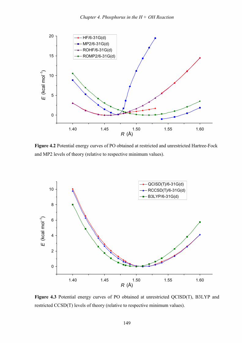
Chapter 4. Phosphorus in the H + OH Reaction
149
-5
0
5
10
15
20
1.35 1.40 1.45 1.50 1.55 1.60R (Å)
E (
kca
l mo
l -1)
HF/6-31G(d)
MP2/6-31G(d)
ROHF/6-31G(d)
ROMP2/6-31G(d)
Figure 4.2 Potential energy curves of PO obtained at restricted and unrestricted Hartree-Fock
and MP2 levels of theory (relative to respective minimum values).
-2
0
2
4
6
8
10
1.35 1.40 1.45 1.50 1.55 1.60R (Å)
E (
kca
l mo
l -1)
QCISD(T)/6-31G(d)
RCCSD(T)/6-31G(d)
B3LYP/6-31G(d)
Figure 4.3 Potential energy curves of PO obtained at unrestricted QCISD(T), B3LYP and
restricted CCSD(T) levels of theory (relative to respective minimum values).

Chapter 4. Phosphorus in the H + OH Reaction
150
of the high level theories RCCSD(T), UQCISD(T) and B3LYP are compared. Overall, the
UQCISD(T) energies closely match the RCCSD(T) values, although a small blip in the
former can now be clearly seen at 1.54 Å. The behaviour of the UB3LYP energies is
completely sensible and predicts an equilibrium PO distance of ~ 1.50 Å, which is ~ 0.015 Å
lower than the RCCSD(T) value.
In light of the above findings the unusual behaviour of the G3 and G3X results is easy to
rationalise. The G3 energies were obtained at the UMP2/6-31G(d) bond distance of 1.4715
Å, that is, just outside the problem region identified above, and thus a seemingly sensible
value for the heat of formation was obtained. The G3X and G3X2 calculations, at the
UB3LYP/6-31G(2df,p) bond distance of 1.4988 Å, are affected by spin contamination. Note,
however, that the UMP2/6-31G(d) value for the bond distance cannot be accepted as reliable,
as the corresponding minimum is largely an artefact of the non physical behaviour of the
UMP2 energy. In contrast with other (well-behaved) P and O containing molecules, where the
MP2 PO distances are typically ~ 0.02 Å longer than the B3LYP values, in PO the UMP2
distance is actually ~ 0.03 Å shorter than the UB3LYP value. Therefore, the seemingly
sensible heat of formation of PO at the G3 level is fortuitous.
4.3.2.2 Comparison with QCISD(T,Full)
As a further test of the G3, G3X and G3X2 methods, the atomisation energies of PO, PO2,
PO3, HPO, HOPO and HOPO2, obtained at the above levels of theory are summarised in
Table 4.3, along with the atomisation energies computed at the QCISD(T,Full) level of theory
using both the G3Large and G3XLarge basis sets, with the higher level correction terms
implicit in the G3 techniques included. Such a comparison of G3 and QCI results is relevant
since the Gaussian methods aim to produce reliable estimates of the QCISD(T,Full) energies
in the largest basis sets used, viz. G3Large and G3XLarge, by applying a series of lower level
quantum chemical methods in conjunction with a range of basis sets. In the case of the PO
and PO2 radicals the standard UHF based results are compared with those obtained by the
appropriate ROHF based techniques. The latter are analogous to Radom’s G3(RAD) and
related methods16-18. Finally, comparisons are also made with Bauschlicher’s (R)CCSD(T)
results44. In all cases G3 reproduces the QCISD(T,Full)/G3Large atomisation energies to
within ~ 1 kcal mol−1, but mostly better. Similarly, G3X2 reproduces the QCISD(T,Full)/

Chapter 4. P
hosphorus in the H +
OH
Reaction
151
Table 4.3 Phosphorus oxides and acids: Comparison of computed atomisation energies (in kcal mol−1).
Atomisation Energy a
PO PO2 PO3 HPO HOPO HOPO2
Method/Reference State UHF ROHF b UHF ROHF b UHF
G3 143.54 143.05 264.15 263.06 360.79 211.92 362.60 480.76
UQCISD(T,Full)/G3largec 143.69 142.36 265.00 263.11 361.69 211.87 362.37 480.84
G3X 146.72 143.66 265.79 264.13 363.39 213.23 364.64 483.51
G3X2 148.10 144.98 268.07 266.15 366.52 215.20 366.71 486.56
UQCISD(T,Full)/G3Xlarged 145.86 144.49 269.43 266.81 368.00 215.50 366.87 487.37
RCCSD(T)/TZ+CVe 135.16 253.10 346.14 204.35 352.11 466.70
RCCSD(T)/QZ+CVe 140.27 261.72 357.74 210.37 361.39 479.97
RCCSD(T)/5Z+CVe 142.12 264.83 361.89 212.39 364.43 na
RCCSD(T)/CBS+CVe 144.05 268.09 366.25 214.51 367.61 489.65
a Not including zero point energy.b All ROHF based calculations performed at UB3LYP/6-31G(2df,p) geometries and use RCCSD(T) in place of QCISD(T) where appropriate.c Including G3 higher level correction.d Including G3X higher level correction.e Including core-valence correlation corrections, Ref. 44.
151

Chapter 4. Phosphorus in the H + OH Reaction
152
G3XLarge atomisation energies to within ~ 1.5 kcal mol−1, except in the case of PO, where
the discrepancy is ~ 2.3 kcal mol−1, for the UHF based calculations. The consistency of the
ROHF based results is significantly better. Comparison with Bauschlicher’s results
demonstrates that the G3X2 method is capable of yielding chemically accurate atomisation
energies and hence heats of formation for this class of difficult molecules. The worst
discrepancy between G3X2 and the CBS results occurs for HOPO2, where the difference is
3.1 kcal mol−1, although at the QCISD(T,Full)/G3XLarge level it is reduced to 2.3 kcal mol−1.
In light of the encouraging performance of the G3X2 method for the above six molecules a
larger systematic evaluation of G3X2 has been undertaken, applying it to a larger number of
phosphorus containing molecules, including all those in Table 4.1. These results are reported
in Chapter 5.
4.4 Kinetic Parameters
A primary aim of this chapter is the calculation of rate coefficients for the PO2 + H and PO2 +
OH recombination reactions (4.1.a) and (4.2.a), and for the subsequent abstraction reactions,
(4.1.b), (4.1.c) and (4.2.b). The rates of these reactions that make up the catalytic cycles are
compared with the (experimental) rates of the (uncatalysed) H + OH recombination reaction
(4.3). The computed geometries of the transition states of these reactions are shown in Figure
4.4. The corresponding heats of formation at 298 K, rotational constants and vibrational
frequencies are summarised in Table 4.4. The geometries of the transition states of reactions
(4.1.b), (4.1.c) and (4.2.b) correspond to well-defined first order saddle points. However, the
recombination reactions (4.1.a) and (4.2.a) are barrierless and thus require a VTST treatment
to locate the geometries of the appropriate transition states at a given temperature, as outlined
in the Sections 2.9.2 and 4.2. The variational transition states were determined at five
temperatures in the range 1000 - 2000 K. The parameters in Figure 4.4 and Table 4.4
pertaining to the transition states of reactions (4.1.a) and (4.2.a) were obtained at 1000 K. The
full set of geometries, rotational constants and vibrational frequencies are given in
Appendices 2.3 and 2.4.

Chapter 4. Phosphorus in the H + OH Reaction
153
Figure 4.4 Geometries of transition states: Variational transition state geometries at 1000 K
for reactions (4.1.a) and (4.2.a) obtained at CASSCF/cc-pVDZ level of theory. All others are
saddle points computed at MP2/6-31G(d) level.
Given the barrierless nature of the recombination reactions (4.1.a) and (4.2.a), the dissociation
rates of HOPO and HOPO2 were initially computed using RRKM at a number of temperatures
in the range 1000 - 2000 K, at pressures 1 - 104 Torr, for a bath gas of N2. The heats of
reactions involving phosphorus containing species were computed using Bauschlicher’s CBS
heats of formation44 (at 298 K) for PO2, HOPO and HOPO2 and experimental literature values
for all other species41-43,45, with the appropriate thermal corrections also taken from JANAF
tabulations41 or computed on the basis of the B3LYP geometries and frequencies44. The rate
coefficients were then fitted to the Troe equations (4.8) - (4.13)35. Figure 4.5 – 4.8 display the
individual rate coefficients and the resulting Troe fits of these. Clearly, the quality of the fits
is generally very good.
O
P O
H
O
P O
H
H
H
O
H
H
P
O
O
O
H
P
O2
O3
O1
H1
H2
2.501
1.497
1.464129.0° 95.6°
0.858
1.310
1.564
1.491
178.9°
122.2°121.4°
1.482 1.481
2.927
0.961
112.0°
1.761
0.979 1.293
0.841
98.8° 167.3°
129.4°
118.7°
1.483 1.487
0.989 1.285
135.7°
112.3°
107.2°
135.3°
Planar
H1-O3-P-O1 = 21.3°H2-O3-P-O1 = -106.8°Planar
PlanarPlanar
1a: H + PO2 → HOPO
2b: H + HOPO2 → H2O + PO22a: OH + PO2 → HOPO2
1c: OH + H2 → H2O +H1b: H + HOPO → H2 + PO2

Chapter 4. P
hosphorus in the H +
OH
Reaction
154
Table 4.4 Computed heats of formation, vibrational frequencies and rotational constants of transition states.a
Reaction ∆ f H2980
Rotational Constants Vibrational Frequencies
/kcal mol−1 /cm−1 /cm−1
1a: H + PO2 → HOPO −20.3 1.2566 0.2936 0.2380 340i 82 152 406 1022 1329
1b: HOPO + H → PO2 + H2 −45.1 1.0019 0.2722 0.2140 2668i 224 270 469 774 787
899 1276 1477
1c: H2 + OH → H2O + H 12.9 18.5846 2.9867 2.5732 2813i 628 675 1283 1443 3602
2a: PO2 +OH → HOPO2 −66.9 0.2919 0.1124 0.0812 200i 86 126 164 426 470
1087 1212 3982
2b: HOPO2 + H → PO2 + H2O −90.2 0.2708 0.2481 0.13213665i
244 279 327 438 530
632 738 1115 1238 1405 3530
a Computed at 1000 K for variational transition states (4.1.a) and (4.2.a).
154

Chapter 4. Phosphorus in the H + OH Reaction
155
-10
-8
-6
-4
-2
0
2
4
6
0.5 0.6 0.7 0.8 0.9 1103/T (K)
log( k
)1 Torr
10 Torr
100 Torr
532 Torr
760 Torr
1000 Torr
10000 Torr
High Pressure Limit
Figure 4.5 Arrhenius plots of RRKM rate constants for HOPO → PO2 + H reaction at a
range of pressures. (Symbols = computed rate constants, Lines = Troe fits.)
-10
-8
-6
-4
-2
0
2
4
0.5 0.6 0.7 0.8 0.9 1103/T (K)
log( k
)
1 Torr
10 Torr
100 Torr
532 Torr
760 Torr
1000 Torr
10000 Torr
High Pressure Limit
Figure 4.6 Arrhenius plots of RRKM rate constants for HOPO2 → PO2 + OH reaction at a
range of pressures. (Symbols = computed rate constants, Lines = Troe fits.)

Chapter 4. Phosphorus in the H + OH Reaction
156
-6
-5
-4
-3
-2
-1
0
-1.0 0.0 1.0 2.0 3.0 4.0
log(p /Torr)
log( k
/ k∞)
1000K
1250K
1500K
1750K
2000K
-6
Figure 4.7 Pressure dependence of RRKM rate constants for HOPO → PO2 + H reaction at a
range of temperatures. (Symbols = computed rate constants, Lines = Troe fits.)
-5
-4
-3
-2
-1
0
-1 0 1 2 3 4
log(p /Torr)
log( k
/ k∞)
1000K
1250K
1500K
1750K
2000K
Figure 4.8 Pressure dependence of RRKM rate constants for HOPO2 → PO2 + OH reaction at
a range of temperatures. (Symbols = computed rate constants, Lines = Troe fits.)

Chapter 4. Phosphorus in the H + OH Reaction
157
The calculated rate coefficients of all the reactions studied in this chapter, in the form of Troe,
Arrhenius or modified Arrhenius fits, are summarised in Table 4.5, in the temperature range
1000 - 2000 K. Further, pertinent computational details of the individual reactions are
discussed below. The rate coefficients of the association (that is, recombination) reactions
were calculated by utilising the appropriate equilibrium constants, as given by Equation (4.7).
The calculated Gibbs free energies of reactions and reaction enthalpies at a number of
temperatures are given in Table 4.6.
HOPO → → → → H + PO2. Initially, the potential energy surfaces of both the cis and trans isomers
were studied in the region of dissociation at the CASSCF/cc-pVDZ level of theory. In the
case of the trans isomer a saddle point was found at an O…H distance of 2.54 Å. This
transition state was ~ 7 kcal mol−1 higher in energy than the dissociation products H + PO2. In
contrast with such a 7 kcal mol−1 barrier to the recombination reaction to give the trans
isomer, no barrier could be found for the dissociation of the lower energy cis isomer. This
indicates that the latter mechanism represents the preferred reaction channel. The geometries
and frequencies of the variational transition states were located at CASSCF/cc-pVDZ level of
theory. As the potential energy surface is very flat in the critical region, the transition state
geometries at the various temperatures show little variation, as the data in Appendices 2.3
and 2.4 indicate. The energies of the transition states relative to the dissociated products were
obtained from CASSCF/cc-pVDZ calculations.
H + HOPO →→→→ H2 + PO2 and OH + H2 →→→→ H2O + H. The transition state geometries
(corresponding to first order saddle points) and critical energies were computed at the G3
level of theory.
HOPO2 →→→→ OH + PO2. The geometries of the variational transition states were located at the
CASSCF/cc-pVDZ level of theory. The energies of the transition states relative to the
dissociated products were calculated at the CASPT2/cc-pVTZ level. As before, the enthalpy
of dissociation was determined using Bauschlicher’s CBS heats of formation (at 298 K) for
PO2 and HOPO2 and experimental values for OH.

Chapter 4. P
hosphorus in the H +
OH
Reaction
158
Table 4.5 Computed rate coefficients: Troea, Arrheniusb and modified Arrheniusb fit parameters.
High pressure limit Low pressure limit
Arrhenius Modified Arrhenius Arrhenius Modified Arrhenius
log A Ea log A n Ea log A Ea log A n Ea
HOPO → PO2 + H 15.34 94.9 13.57 0.50 93.6 16.57 82.1 34.97 −5.13 96.1
PO2 + H → HOPO 10.06 1.29 −1.5 31.46 −4.33 1.02
HOPO + H → H2 + PO2 c 14.28 16.1 7.33 1.94 10.8
H2 + OH → H2O + H c 14.33 9.9 5.92 2.34 3.5
HOPO2 → HO + PO2 15.56 105.2 24.44 −2.48 112.0 18.41 91.5 57.26 −10.83 121.0
HO + PO2 → HOPO2 14.19 −0.24 0.0 47.01 −8.59 9.0
HOPO2 + H → PO2 + H2O c 14.10 26.7 8.74 1.49 22.6
Troe Fit
a 1−a T* T** T***
HOPO → PO2 + H 1.00 0.00 950.72 4797.20 −115.31
PO2 + H → HOPO
HOPO + H → H2 + PO2 c
H2 + OH → H2O + H c
HOPO2 → HO + PO2 1.00 −2.22×10⁻⁶ 640.64 3973.10 −202.75
HO + PO2 → HOPO2
HOPO2 + H → PO2 + H2O c
a See equations (8) - (13); T*, T**, T*** in K.b See equations (5) and (6); Ea in kcal mol−1, A in s−1 or cm3 mol−1 s−1.
c These reactions are not pressure dependent.
158

Chapter 4. Phosphorus in the H + OH Reaction
159
Table 4.6 Computed enthalpies and Gibbs free energies of reaction (in kcal mol−1) at a range
of temperatures.
H + PO2 → HOPO OH + PO2 → HOPO2
T /K 0Tr H∆ 0
TrG∆ 0Tr H∆ 0
TrG∆298.15 −94.2 −86.6 −110.4 −99.1
1000 −95.4 −67.4 −110.0 −72.4
1250 −95.6 −60.4 −109.5 −63.1
1500 −95.7 −53.4 −108.9 −53.9
1750 −95.7 −46.3 −108.3 −44.7
2000 −95.7 −39.3 −107.6 −35.7
H + HOPO2 →→→→ H2O + PO2. The search for a transition state for this reaction initially yielded
a minimum corresponding to a weakly bound PO2…H2O dimer. This dimer had a binding
energy of 4.8 kcal mol−1 after applying the counterpoise correction for basis set superposition
effects. However, from the point of view of this work the existence of such a dimer is of
academic interest only as it would not be expected to be stable at ~ 2000 K. The transition
state for OH abstraction by H is characterised by a long OH bond and a slightly elongated PO
bond. The geometry and barrier height were located at the G3 level of theory.
Finally, the calculated rate coefficients at the temperatures of 1000 and 2000 K and a pressure
of 532 torr are summarised in Table 4.7 where they are compared with Twarowski’s
estimated values (which were obtained by the application of Benson’s rules), the modelling
values of Korobeinichev et al.13 and experiment.47
At 2000 K the rate coefficients in the two reaction schemes considered are comparable in
magnitude, suggesting that both routes are important, in qualitative agreement with
Twarowski’s conclusions. However, in an absolute sense, the rate coefficients obtained in this
work are significantly lower than Twarowski’s, especially at 1000 K, although order of
magnitude differences can exist even at the higher temperature. Our values agree somewhat
better with the modelled values of Korobeinichev et al.,13 but there remain significant
differences. Under the conditions studied by Twarowski (0.7 atm pressure and 1970 K) the
rate coefficient for (4.1.a) is substantially into falloff (approximately 1,000 fold lower than the
high pressure limit), whereas the coefficient for (4.2.a) is significantly less so (only ~ 60 fold

Chapter 4. P
hosphorus in the H +
OH
Reaction
160
Table 4.7 Comparison of computed and experimental rate coefficients at 532 Torr pressure at 1000 and 2000 K (in cm3mol−1s−1).
Reaction T (K) k (This work) k (Twarowskia) k (Korobeinichev et al.b) k (expt.)
1a: PO2 + H → HOPO 1000 7.03×10¹² 4.42×10¹² c4.55×1013 c
2000 2.78×10¹¹ 2.87×10¹¹ c6.51×1012 c
1b: HOPO + H → H2 + PO2 1000 6.08×10¹⁰ 3.15×10¹³ 7.7×10¹¹
2000 3.53×10¹² 3.16×10¹³ 7.8×10¹¹
1c: H2 + OH → H2O + H 1000 1.52×10¹² 6.28×10¹³ 1.26×10¹² d
2000 1.88×10¹³ 6.30×10¹³ 8.33×10¹² d
2a: HO + PO2 → HOPO2 1000 7.40×10¹² 1.74×10¹⁴ c1.71×1013 c
2000 3.68×10¹¹ 5.62×10¹² c1.89×1012 c
2b: HOPO2 + H → PO2 + H2O 1000 1.93×1081 3.16×10¹³ 1.55×1091
2000 1.60×10¹¹ 3.16×10¹³ 3.13×10¹⁰
3: H + OH → H2O 1000 3.56×1091 c7.12×1012 c,e
2000 1.17×1091 c8.91×1091 c,e
a Ref. 3.b Ref. 13.c Calculated as k[M].d Fit to all NIST data, Ref. 48.e Ref. 47.
160

Chapter 4. Phosphorus in the H + OH Reaction
161
lower than the high pressure limit). Thus, whilst it might be acceptable to use the termolecular
rate coefficient for (4.1.a) in modelling, in light of its proximity to the limiting low pressure
value, the appropriate falloff value of the rate coefficient should be used for (4.2.a). For the
H2 + OH abstraction reaction (4.1.c) the computed G3 rate coefficients agree with the
observed values48 to within a factor of approximately two or better, depending on the
temperature.
4.5 Conclusion
Using ab initio quantum chemical and RRKM techniques, theoretical rate coefficients were
obtained for the H + PO2 (4.1.a) and OH + PO2 (4.2.a) recombination reactions and for the
subsequent H + HOPO (4.1.b) and H + HOPO2 (4.2.b) abstraction reactions, which, along
with the OH + H2 abstraction reaction (4.1.c) constitute the catalytic pathway for the H + OH
recombination reaction (4.3), as formulated by Twarowski1-4 and also by Korobeinichev et
al.13 The computed rate coefficients for (4.1.c) agree well with experiment (within 20% at
1000 K and almost within a factor of 2 at 2000 K), while for the other reactions the rate
coefficients are consistent with the modelled values of Korobeinichev et al.,13 although for
several key reactions ((4.1.b), (4.2.a), (4.2.b)) they are substantially lower than Twarowski’s
values. Whilst we utilised Bauschlicher’s44 recent thermochemical data in the derivation of
our rate coefficients, we note that reasonable accuracy could be achieved by the application of
the G3X and G3X2 methods to the computation of the heats of formation of the phosphorus
containing species. Using the G2, G3 and G3X methods we also computed the
thermochemistry of Twarowski’s reaction model which includes 17 phosphorus containing
molecules.

Chapter 4. Phosphorus in the H + OH Reaction
162
4.6 References
1. A. Twarowski, Combustion and Flame, 1993, 94, 91.
2. A. Twarowski, Combustion and Flame, 1993, 94, 341.
3. A. Twarowski, Combustion and Flame, 1995, 102, 41.
4. A. Twarowski, Combustion and Flame, 1996, 105, 407.
5. S. W. Benson, Thermochemical Kinetics; John Wiley: New York, NY, 1976.
6. L. A. Curtiss, K. Raghavachari, G. W. Trucks and J. A. Pople, J. Chem. Phys., 1991,
94, 7221.
7. L. A. Curtiss, K. Raghavachari, P. C. Redfern, V. Rassolov and J. A. Pople, J. Chem.
Phys., 1998, 109, 7764.
8. L. A. Curtiss, P. C. Redfern, K. Raghavachari and J. A. Pople, J. Chem. Phys., 2001,
114, 108.
9. M. A. MacDonald, T. M. Jayaweera, E. M. Fisher and F. C. Gouldin, Combustion and
Flame, 1999, 116, 166.
10. J. Green, Fire Sciences, 1996, 14, 426.
11. C. R. Dempsey and E. T. Oppelt, Air and Waste, 1993, 43, 25.
12. O. P. Korobeinichev, S. B. Ilyin, T. A. Bolshova, V. M. Shvartsberg and A. A.
Chernov, Combustion and Flame, 2000, 121, 593.
13. O. P. Korobeinichev, T. A. Bolshova, V. M. Shvartsberg and A. A. Chernov,
Combustion and Flame, 2001, 125, 744.
14. M. A. MacDonald, F. C. Gouldin and E. M. Fisher, Combustion and Flame, 2001,
124, 668.
15. L. A. Curtiss, K. Raghavachari, P. C. Redfern and J. A. Pople, J. Chem. Phys., 1997,
106, 1063.
16. D. J. Henry and L. Radom, in Theoretical Thermochemistry. J. Cioslowski, Ed.;
Kluwer: Dordrecht, 2001.
17. P. M. Mayer, C. J. Parkinson, D. M. Smith and L. Radom, J. Chem. Phys., 1998, 108,
604.
18. C. J. Parkinson, P. M. Mayer and L. Radom, J. Chem. Soc., Perkin Trans. 2, 1999, 11,
2305.
19. J. A. Pople, M. Head-Gordon and K. Raghavachari, J. Chem. Phys., 1987, 87, 5968.

Chapter 4. Phosphorus in the H + OH Reaction
163
20. K. Raghavachari, G. W. Trucks, J. A. Pople and M. Head-Gordon, Chem. Phys. Lett.,
1989, 157, 479.
21. C. Hampel, K. A. Peterson and H.-J. Werner, Chem. Phys. Lett., 1992, 190, 1.
22. J. I. Steinfeld, J. S. Francisco and W. L. Hase, Chemical Kinetics and Dynamics;
Prentice Hall: Engelwood Cliffs, NJ, 1989, 308.
23. D. A. McQuarrie, Statistical Mechanics; Harper & Row: New York, 1973, 129.
24. E. Pollack, in Theory of Chemical Reaction Dynamics. M. Baer, Ed.; Vol. 3; CRC
Press: Boca Raton, 1985, p. 128.
25. D. G. Truhlar and B. C. Garrett, Acc. Chem. Res., 1980, 13, 440.
26. W. L. Hase, S. L. Mondro, R. J. Duchovic and D. M. Hirst, J. Am. Chem. Soc., 1987,
109, 2916.
27. G. B. Bacskay, M. Martoprawiro and J. C. Mackie, Chem. Phys. Lett., 1999, 300, 321.
28. K. Sendt, G. B. Bacskay and J. C. Mackie, J. Phys. Chem. A, 2000, 104, 1861.
29. B. O. Roos, P. R. Taylor and P. E. M. Siegbahn, Chem. Phys., 1980, 48, 157.
30. B. O. Roos, in Ab initio Methods in Quantum Chemistry II. K. P. Lawley, Ed.; J.
Wiley & Sons Ltd.: Chichester, UK, 1987, p. 399.
31. T. H. Dunning, Jr., J. Chem. Phys., 1989, 90, 1007.
32. D. E. Woon and T. H. Dunning, Jr., J. Chem. Phys., 1993, 98, 1358.
33. K. Andersson, P.-Å. Malmqvist, B. O. Roos, A. J. Sadlej and K. Wolinski, J. Phys.
Chem., 1990, 94, 5483.
34. K. Andersson, P.-Å. Malmqvist and B. O. Roos, J. Chem. Phys., 1992, 96, 1218.
35. R. G. Gilbert, K. Luther and J. Troe, Ber. Bunsenges. Phys. Chem., 1983, 87, 169.
36. M. J. Frisch, G. W. Trucks, H. B. Schlegel, G. E. Scuseria, M. A. Robb, J. R.
Cheeseman, V. G. Zakrzewski, J. A. Montgomery, R. E. Stratmann, J. C. Burant, S.
Dapprich, J. M. Millam, A. D. Daniels, K. N. Kudin, M. C. Strain, O. Farkas, J.
Tomasi, V. Barone, M. Cossi, R. Cammi, B. Mennucci, C. Pomelli, C. Adamo, S.
Clifford, J. Ochterski, G. A. Petersson, P. Y. Ayala, Q. Cui, K. Morokuma, D. K.
Malick, A. D. Rabuck, K. Raghavachari, J. B. Foresman, J. Cioslowski, J. V. Ortiz, B.
B. Stefanov, G. Lui, A. Liashenko, P. Piskorz, I. Komaromi, R. Gomperts, R. L.
Martin, D. J. Fox, T. Keith, M. A. Al-Laham, C. Y. Peng, A. Nanayakkara, C.
Gonzalez, M. Challacombe, P. M. W. Gill, B. G. Johnson, W. Chen, M. W. Wong, J.
L. Andres, M. Head-Gordon, E. S. Replogle and J. A. Pople, Gaussian 98 (Revision
A.7), Gaussian, Inc.: Pittsburgh, PA, 1998.

Chapter 4. Phosphorus in the H + OH Reaction
164
37. ACES II is a program product of the Quantum Theory Project, University of Florida.
Authors: J. F. Stanton, J. Gauss, J. D. Watts, M. Nooijen, N. Oliphant, S. A. Perera, P.
G. Szalay, W. J. Lauderdale, S. R. Gwaltney, S. Beck, A. Balková, D. E. Bernholdt,
K.-K. Baeck, P. Rozyczko, H. Sekino, C. Hober, R. J. Bartlett. Integral packages
included are VMOL (J. Almlöf and P. R. Taylor); VPROPS (P. Taylor); ABACUS (T.
Helgekar, H. J. Aa. Jensen, P. Jørgensen, J. Olsen and P. R. Taylor).
38. "DALTON, an ab initio electronic structure program, Release 1.0 (1997)" written by
T. Helgaker, H. J. Aa. Jensen, P. Jørgensen, J. Olsen, K. Ruud, H. Ågren, T.
Andersen, K. L. Bak, V. Bakken, O. Christiansen, P. Dahle, E. K. Dalskov, T.
Enevoldsen, B. Fernandez, H. Heiberg, H. Hettema, D. Jonsson, S. Kirpekar, R.
Kobayashi, H. Koch, K. V. Mikkelsen, P. Norman, M. J. Packer, T. Saue, P. R. Taylor
and O. Vahtras.
39. K. Andersson, M. R. A. Blomberg, M. P. Fülscher, G. Karlström, R. Lindh, P.-Å.
Malmqvist, P. Neogrády, J. Olsen, B. O. Roos, A. J. Sadlej, M. Schültz, L. Seijo, L.
Serrano-Andrés, P. E. M. Siegbahn and P.-O. Widmark, MOLCAS (Version 4), Lund
University: Lund, Sweden, 1997.
40. V. Mokrushin, V. Bedanov, W. Tsang, M. Zachariah and V. Knyazev, Chemrate
(1.10), National Institute of Standards and Technology: Gaithersburg, MD, USA,
1999.
41. M. W. Chase, Jr., J. Phys. Chem. Ref. Data, 1998, Monograph 9, 1.
42. B. Rusic, D. Feller, D. A. Dixon, K. A. Peterson, L. B. Harding, R. L. Asher and A. F.
Wagner, J. Phys. Chem. A, 2001, 105, 1.
43. J. Drowart, C. E. Myers, R. Szwarc, A. Vander Auwera-Mahieu and O. M. Uy, J.
Chem. Soc., Faraday Trans. 2, 1972, 68, 1749.
44. C. W. Bauschlicher, Jr., J. Phys. Chem. A, 1999, 103, 11126.
45. D. L. Hildenbrand and K. H. Lau, J. Chem. Phys., 1994, 100, 8373.
46. L. A. Curtiss, K. Raghavachari, P. C. Redfern and J. A. Pople, J. Chem. Phys., 2000,
112, 7374.
47. D. L. Baulch, C. J. Cobos, R. A. Cox, C. Esser, P. Frank, T. Just, J. A. Kerr, M. J.
Pilling, J. Troe, R. W. Walker and J. Warnatz, J. Phys. Chem. Ref. Data, 1992, 21,
411.
48. W. G. Mallard, F. Westley, J. T. Herron, R. G. Hampson and D. H. Frizzell, NIST
Chemical Kinetic Database: Version 2Q98. 1998, National Institute of Standards and
Technology, Gaithersburg, MD.

5 Accurate Thermochemistry of Phosphorus Compounds
Chapter 5
Accurate
Thermochemistry
of Phosphorus
Compounds

Chapter 5. Accurate Phosphorus Thermochemistry
166
5.1 Introduction
During the last decade a considerable degree of interest has developed in phosphorus
containing molecules as potential catalysts, with the ability to accelerate a range of radical
recombination reactions.1-7 Such catalytic activity has implications in a number of fields, such
as flame suppression, engine fuel efficiency and nerve gas disposal. Unfortunately, the
development of reliable kinetic models for these processes has been hampered by a lack of
accurate thermochemical and kinetic data. The work reported in this chapter aims to aid in
remedying this problem by undertaking the computation of accurate heats of formation for a
number of small phosphorus-containing molecules using current techniques of computational
quantum chemistry.
As in other work8-17 concerned with the ab initio computation of thermochemistry, the
approach here has been to compute the atomisation energies and hence heats of formation of
the molecules of interest by the application of the CCSD(T) coupled cluster method in
conjunction with correlation consistent basis sets (aug)-cc-pVxZ (x = T, Q, 5), followed by
extrapolation to the complete basis set (CBS) limit, and inclusion of corrections for core-
valence correlation, spin-orbit coupling and scalar relativistic effects. Such calculations have
already been reported by Bauschlicher15 for PO, PO2, PO3, HPO, HOPO and HOPO2. In
addition to these phosphorus oxides and acids, heats of formation for P2, P4, PH, PH2, PH3,
P2H2, P2H4, P2O, P2O2, HPOH, H2POH, and H3PO have been calculated and are reported here.
Regarding the computed CCSD(T)/CBS thermochemistry as a benchmark, the second aspect
of this work is a critical test of Gaussian-3 type methods, in particular G318, G3X19 and
G3X220, when applied to the above set of molecules. As these techniques are considerably
less computer resource intensive than the CCSD(T)/CBS approach, they would have a wider
range of applicability, especially for larger systems. However, given that the original test set
of molecules that was used to calibrate the G3 and G3X methods contains comparatively few
phosphorus containing species (due largely to the lack of reliable experimental information),
an assessment of the capability and reliability of these methods for a larger number of
phosphorus containing molecules is clearly desirable.

Chapter 5. Accurate Phosphorus Thermochemistry
167
The heats of formation of the above phosphorus compounds, as calculated by G3 and G3X,
have been reported in the previous chapter (and also published20), although the main focus of
that work was the computation of rate coefficients for the H + PO2 and OH + PO2
recombination reactions and for the H + HOPO → H2 + PO2, OH + H2 → H + H2O, and H +
HOPO2 → H2 + PO2 abstraction reactions, which constitute a catalytic pathway for the H +
OH recombination reaction. Comparison of the G3 and G3X heats of formation with the
CCSD(T)/CBS values of Bauschlicher for the six phosphorus oxides and acids PO, PO2, …
HOPO2 revealed that the G3 and G3X heats of formation were in error by up to ~ 9 and 6 kcal
mol−1 respectively, given that the CCSD(T)/CBS values are believed to be essentially
chemically accurate, with estimated errors of ~ 1 kcal mol−1. The performance of G3X2 was
found to be superior to G3X, with the maximum deviation from the CCSD(T)/CBS values
being ~ 3 kcal mol−1.) Extending such comparisons to a larger set of molecules, as undertaken
in this study, is seen as definitely warranted.
This work, therefore, has two primary aims: firstly to generate benchmark atomisation
energies (AE) and heats of formation for a larger selection of small phosphorus containing
molecules and secondly to use these results to assess the reliability of the G3 type methods for
these systems.
5.2 Theory And Computational Methods
The application of coupled cluster theory in conjunction with correlation consistent basis sets
and extrapolation to the CBS limit has become well established as a reliable approach for
generating accurate heats of formation from atomisation energies.8-17 This is the scheme that
was employed by Bauschlicher15 to calculate thermochemical data for the phosphorus oxides
and acids. The approach here for the generation of benchmark heats of formation is
effectively the same as Bauschlicher’s.
The geometries and vibrational frequencies in this work were obtained using density
functional theory, employing the B3LYP exchange-correlation functional21-24 and the
6-31G(2df,p) basis set, as prescribed by G3X theory (with a scale factor of 0.9854 for the
computation of zero point energies). This basis set is somewhat different from those used by

Chapter 5. Accurate Phosphorus Thermochemistry
168
Bauschlicher, viz. 6-31+G(2df) for geometries and 6-31G(d) for frequencies. The single point
energy calculations at the B3LYP optimised equilibrium geometries were performed using
coupled cluster theory with single and double excitations, with the inclusion of triples by
perturbation theory (CCSD(T))25,26. The open shell reference state orbitals and energies were
generated by restricted Hartree-Fock (RHF) theory, while the subsequent coupled cluster
energies were obtained by the restricted RCCSD(T) method.
The basis sets employed in the sequence of valence-correlated coupled cluster calculations
(where the 1s electrons on O and 1s, 2s, 2p electrons on P are left uncorrelated) are the
correlation consistent valence-polarised (cc-pV) triple-ζ (TZ), quadruple-ζ (QZ) and
pentuple-ζ (5Z) basis sets developed by Dunning et al.27-29 As recommended by
Bauschlicher15, an additional tight d function was added to each of the phosphorus basis sets
with an exponent three times that of the largest d function in the original set (that is, 1.956,
3.11 and 8.00 for the TZ, QZ and 5Z sets respectively). Diffuse functions were also included
in the oxygen basis sets; that is, for O atoms the aug-cc-pVxZ basis sets27,28 are used. The
resulting basis sets for molecules with P, O and H atoms are denoted (aug-)cc-pVxZ+d.
The three valence (R)CCSD(T) single point energies were then extrapolated to the CBS limit
({T,Q,5}). All four extrapolation schemes mentioned in Section 2.7.3 were employed; that is,
the mixed exponential/Gaussian extrapolation of Feller30 (“mix”, Equation (5.1)), the
Schwartz type extrapolations31 (“ maxl ”, Equation (5.2) and “ 4 6n n− −+ ”, Equation (5.3)) and
the “ 3x− ” scheme of Helgaker et al.16 (Equation (5.4)).
( ) ( ) ( )( )2exp 1 exp 1E x A B x C x= + − + − − (5.1)
( ) ( ) 4
max 1 2E x A B l−= + + (5.2)
( ) ( ) ( )4 6
max max1 2 1 2E x A B l C l− −= + + + + (5.3)
( ) 3E x A Bx−= + (5.4)

Chapter 5. Accurate Phosphorus Thermochemistry
169
The core-valence (and core-core) correlation energies (CV) were computed via (R)CCSD(T)
calculations using both the correlation consistent polarised core valence triple-ζ (cc-pCVTZ)
basis sets of Dunning et al.27,29,32 (aug-cc-pCVTZ for oxygen) as well as the core-valence
basis sets proposed by Bauschlicher15. The CV contributions to the atomisation energies were
corrected for basis set superposition effects (BSSE) by application of the counterpoise (CP)
method of Boys and Bernardi33. The CP treatment was restricted to the phosphorus atoms of
any given molecule; that is, CP corrections to the CV component of the energies, denoted
CP(CV), were computed only for the P atoms.
The spin-orbit coupling energy corrections for the atomic species were taken from the
tabulation of Curtiss et al.18 The only molecule in the set which would be expected show
appreciable spin-orbit coupling is PO; in this case the value calculated by Bauschlicher15 was
used. Scalar relativistic corrections, viz. the Darwin and mass-velocity contributions34,35, were
calculated using finite field perturbation theory, utilising the complete active space second
order perturbation theory (CASPT2) method36,37 with complete active space self-consistent
field (CASSCF)38,39 reference states, and the G3Large basis sets of Curtiss et al.18
The Gaussian methods, G140, G241, G318 and their variants42-46, have been designed to
approximate a molecular energy that would result from the application of a high level of
quantum chemical theory in conjunction with a large basis set by a series of lower level
calculations and/or smaller basis sets. This, of course, results in significant savings of
computer resources. The G3 and G3X methods have already been described in detail in
Section 2.7.2. In brief, in G3 the aim is to effectively reproduce the electronic energy of a
QCISD(T, Full) calculation obtained with the G3Large basis set.
[ ] [ ][ ] [ ]{ }[ ] [ ]{ }[ ] [ ]
[ ] [ ]
0 G3 QCISD(T)/6-31G( )
MP4/6-31 G( ) MP4/6-31G( ) ( correction)
MP4/6-31G(2 , ) MP4/6-31G( ) (2 , correction)
MP2(Full)/G3Large MP2/6-31G(2 , )(G3La
MP2 6-31 G MP2 6-31G
E E d
E d E d
E df p E d df p
E E df p
E d E d
=
+ + − +
+ −
− + − / + ( ) + / ( )
ZPE SO hlc
rge correction)
E E E+ ∆ + ∆ + ∆
(5.5)

Chapter 5. Accurate Phosphorus Thermochemistry
170
G3X theory is a derivative of G3, designed primarily so as to improve agreement between
theoretical and experimental heats of formation for molecules which contain second row
atoms (Na-Ar). This is achieved by using improved geometries and vibrational frequencies
and by the inclusion of a so-called G3XLarge correction at the SCF level using the G3XLarge
basis set:
[ ] [ ] [ ] [ ]{ }0 0G3X G3 HF/G3XLarge HF/G3Large
G3XLarge correction
E E E E= + − (5.6)
(with the understanding that the equilibrium geometry and zero point vibrational correction
are obtained by B3LYP/6-31G(2df,p) calculations).
The recently proposed G3X2 method (Section 2.7.2.5, Chapter 4) differs from G3X only in
that the G3XLarge correction is now evaluated using MP2(Full):
[ ] [ ] [ ] [ ]{ }0 0G3X2 G3 MP2(Full)/G3XLarge MP2(Full)/G3LargeE E E E= + − (5.7)
The G3X2 approach can also be regarded as a G3 calculation (with the geometry and zero
point energy correction determined at the B3LYP/6-31G(2df,p) level) where the G3Large
basis has been replaced by the G3XLarge set:
[ ] [ ][ ] [ ]{ }[ ] [ ]{ }[ ] [ ]
[ ] [ ]
0 G3X2 QCISD(T)/6-31G( )
MP4/6-31 G( ) MP4/6-31G( ) ( correction)
MP4/6-31G(2 , ) MP4/6-31G( ) (2 , correction)
MP2(Full)/G3XLarge MP2/6-31G(2 , )(G
MP2 6-31 G MP2 6-31G
E E d
E d E d
E df p E d df p
E E df p
E d E d
=
+ + − +
+ −
− + − / + ( ) + / ( )
ZPE SO hlc
3X2 correction)
E E E+ ∆ + ∆ + ∆
(5.8)
G3X2 represents an approximation to a QCISD(T,Full)/G3XLarge computation and, as it
accounts for a greater degree of electron correlation energy than G3X, it is reasonable to
expect that it would be superior to G3X in an absolute sense, that is, yield closer agreement
with experiment. Indeed, as remarked in the introduction to this chapter (Section 5.1), we

Chapter 5. Accurate Phosphorus Thermochemistry
171
found that for the six phosphorus oxides and acids PO, PO2, … HOPO2 studied by
Bauschlicher the G3X2 heats of formation were in significantly better agreement with
Bauschlicher’s CCSD(T)/CBS values than those obtained by G3X.
A further suggested refinement of G3X2 which is introduced in this work is to correct the CV
component of the energy for BSSE, which can be quite large for phosphorus containing
molecules. The analogous corrections for BSSE effects within the valence space are assumed
to be taken care of by the higher level corrections. In G3X2 the latter are defined the same
way as in G3X, that is, in terms of the valence electrons of a given molecules, according to
Equations (2.7.12) and (2.7.13). While ultimately the parameters A, B, C and D would need to
be reoptimised for G3X2, no such optimisation has been undertaken here, as there are too few
molecules in our data set for such results to have wider applicability. Therefore, the hlc
parameters of G3X, given in Section 2.7.2.4, have been adopted for the current
implementation of G3X2.
The standard Gaussian theories treat open shell systems (atoms and molecules) by the
unrestricted methods: UHF, UMP2, UMP4 and UQCISD(T). An alternative approach is the
Gn(RAD) type approach of Radom and co-workers47-49, where the UHF and UMP
computations are replaced by their restricted open shell ROHF and ROMP analogues and
RCCSD(T) is used instead of the UQCISD(T) method implicit in G2 and G3. In this work
both the standard (unrestricted) formulation of G3X2 as well as the (restricted) G3X2(RAD)
procedure have been used for all atoms as well as several open shell molecules.
The B3LYP geometries and vibrational frequencies as well as the G3X2 energies were
generated using the Gaussian98 suite of programs50. The (R)CCSD(T) and ROMP
calculations were performed with MOLPRO26,51,52 and ACESII53 respectively. The CASSCF
and CASPT2 calculations of the scalar relativistic corrections were carried out using
MOLCAS54. The computations were performed on DEC alpha 600/5/333 and COMPAQ
XP100/500 workstations of the Theoretical Chemistry group at the University of Sydney and
on the COMPAQ AlphaServer SC system of the Australian Partnership for Advanced
Computing National Facility at the National Supercomputing Centre, ANU, Canberra.

Chapter 5. Accurate Phosphorus Thermochemistry
172
5.3 Results and Discussion
5.3.1 CCSD(T) Benchmark Calculations
The geometric parameters, rotational constants and vibrational frequencies of the species
studied in this investigation can be found in Appendix 2.1.
Table 5.1 contains the absolute energies of the molecules of interest and their component
atoms, as obtained at the highest level of (valence) correlated theory, namely (R)CCSD(T)/
(aug-)cc-pV5Z+d, along with the {T,Q,5} 3x− extrapolated energies, CV correlation
corrections, CP corrections for BSSE in the latter, zero point vibrational energies, thermal
corrections to the enthalpies and the scalar relativistic energy corrections.
5.3.1.1 Testing the B3LYP Geometry
As a test of the reliability of the B3LYP functional for the computation of molecular
geometries, P4 was taken as test case and its equilibrium geometry re-computed using
CCSD(T). The results are summarised in Figure 5.1 which shows the computed molecular
energy as a function of the P-P distance in tetrahedral P4. The B3LYP and valence correlated
CCSD(T) calculations yield effectively the same geometry, but a shorter bond length is
obtained when the CCSD(T) calculations include CV correlation. (The force constants from
these three calculations are comparable.) These findings are interesting, since the DFT
calculations do include CV correlation. In the context of the current work, however, the
discrepancy in the B3LYP geometry is negligible, as the resulting error in the molecular
energy is only ~ 0.04 kcal mol−1. As in this work P4 is probably the most difficult molecule to
describe accurately, it is expected that any inaccuracies in the molecular energies of other
species, resulting from errors in the choice of equilibrium geometries will be similarly
negligible.
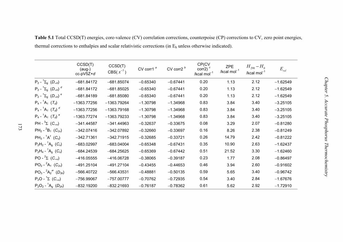
Chapter 5. A
ccurate Phosphorus T
hermochem
istry
173
Table 5.1 Total CCSD(T) energies, core-valence (CV) correlation corrections, counterpoise (CP) corrections to CV, zero point energies,
thermal corrections to enthalpies and scalar relativistic corrections (in Eh unless otherwise indicated).
CCSD(T)
(aug-)cc-pV5Z+d
CCSD(T)
CBS( 3x− )CV corr1 a CV corr2 b
CP(CVcorr2) c
/kcal mol−1
ZPE/kcal mol−1
298 0H H−/kcal mol−1 relE
P2 - 1Σg (D∞h) −−681.84172 −−681.85074 −0.65340 −0.67441 0.20 −1.13 2.12 −1.62549
P2 - 1Σg (D∞h)
d −−681.84172 −−681.85025 −0.65340 −0.67441 0.20 −1.13 2.12 −1.62549
P2 - 1Σg (D∞h)
e −−681.84189 −−681.85080 −0.65340 −0.67441 0.20 −1.13 2.12 −1.62549
P4 - 1A1 (Td) −1363.77256 −1363.79264 −1.30798 −1.34968 0.83 −3.84 3.40 −3.25105
P4 - 1A1 (Td)
d −1363.77256 −1363.79168 −1.30798 −1.34968 0.83 −3.84 3.40 −3.25105
P4 - 1A1 (Td)
e −1363.77274 −1363.79233 −1.30798 −1.34968 0.83 −3.84 3.40 −3.25105
PH - 3Σ (C∞v) −−341.44587 −−341.44963 −0.32637 −0.33675 0.08 −3.29 2.07 −0.81280
PH2 - 2B1 (C2v) −−342.07416 −−342.07892 −0.32660 −0.33697 0.16 −8.26 2.38 −0.81249
PH3 - 1A′ (Cs) −−342.71361 −−342.71915 −0.32685 −0.33721 0.26 14.79 2.42 −0.81222
P2H2 - 1Ag (Cs) −−683.02997 −−683.04004 −0.65348 −0.67431 0.35 10.90 2.63 −1.62437
P2H4 - 1Ag (Cs) −−684.24539 −−684.25625 −0.65369 −0.67442 0.51 21.52 3.30 −1.62460
PO - 2Σ (C∞v) −−416.05555 −−416.06728 −0.38065 −0.39187 0.23 −1.77 2.08 −0.86497
PO2 - 2A1 (C2v) −−491.25104 −−491.27104 −0.43455 −0.44653 0.46 −3.94 2.60 −0.91602
PO3 - 2A2″ (D3h) −−566.40722 −−566.43531 −0.48881 −0.50135 0.59 −5.65 3.40 −0.96742
P2O - 1Σ (C∞v) −−756.99067 −−757.00777 −0.70762 −0.72935 0.54 −3.40 2.84 −1.67676
P2O2 - 1Ag (D2h) −−832.19200 −−832.21693 −0.76187 −0.78362 0.61 −5.62 2.92 −1.72910
173

Chapter 5. A
ccurate Phosphorus T
hermochem
istry
174
Table 5.1. continued
CCSD(T)
(aug-)cc-pV5Z+d
CCSD(T)
CBS( 3x− )CV corr1 a CV corr2 b
CP(CVcorr2) c
/kcal mol−1
ZPE/kcal mol−1
298 0H H−/kcal mol−1 relE
HPO - 1A′ (Cs) −−416.66743 −−416.67983 −0.38068 −0.39180 0.29 −6.09 2.40 −0.86449
HPOH - 2A″ (Cs) −−417.26372 −−417.27646 −0.38084 −0.39176 0.25 13.39 2.63 −0.86372
H2POH - 1A′ (Cs) −−417.89452 −−417.90796 −0.38095 −0.39183 0.33 19.43 2.81 −0.86396
H3PO - 1A1 (C3v) −−417.89612 −−417.91002 −0.38055 −0.39161 0.45 19.07 2.51 −0.86326
HOPO - 1A′ (Cs) −−491.90932 −−491.92982 −0.43510 −0.44683 0.38 10.95 2.77 −0.91634
HOPO2 - 1A′ (Cs) −−567.13090 −0.48901 −0.50149 0.59 14.36 3.13 −0.96707
H −−−−0.49999 −−−−0.50005 −0.00000 −0.00000 1.01 −0.00000
O −−−75.00041 −−−75.00653 −0.05354 −0.05414 1.04 −0.05230
P −−340.82973 −−340.83229 −0.32617 −0.33656 1.28 −0.81296
P d −−340.82973 −−340.83208 −0.32617 −0.33656 1.28 −0.81296
P e −−340.82980 −−340.83235 −0.32617 −0.33656 1.28 −0.81296
a Calculated using Dunning’s cc-pCVnZ basis sets, Refs 27, 29, 32.b Calculated using Bauschlicher’s core-valence basis sets, Ref. 15.c Counterpoise correction for BSSE on P atoms in CV corr2.d Extrapolation process includes the cc-pV6Z+d energy.e Calculated using cc-pCV(n+d)Z basis sets, Ref. 56.
174

Chapter 5. Accurate Phosphorus Thermochemistry
175
Figure 5.1 P4: Comparison of computed equilibrium geometries and potential energy surfaces
with respect to the symmetric stretch.
5.3.1.2 Atomisation Energies and Extrapolation Schemes
It is generally recognised that atomisation energies provide a far more convenient tool than
absolute energies for investigating the merits of the various extrapolation schemes and the
relative magnitudes of the corrections involved in the calculations of thermochemistry.
Therefore a range of these, as obtained with all three basis sets used for valence correlated
calculations (triple-, quadruple- and pentuple-ζ) and all four extrapolation methods, along
with the CV and scalar relativistic corrections are listed in Table 5.2. We note here that in the
case of HOPO2 the RCCSD(T)/(aug-)cc-pV5Z+d calculation proved too demanding for our
computing resources and for this molecule therefore, as in Bauschlicher’s work, the
extrapolations (for HOPO2 and its atoms) are based on the triple- and quadruple-ζ energies
alone ({T,Q}). (This necessarily means that only the maxl and 3x− extrapolation schemes
could be implemented for HOPO2.) Bauschlicher expressed some concern about this in his
paper, stating that the two-point {T,Q} extrapolation is likely to result in an overestimation of
the atomisation energy by 0.85 kcal mol−1.
-0.02
0.00
0.02
0.04
0.06
0.08
0.10
2.198 2.200 2.202 2.204 2.206 2.208 2.210 2.212 2.214 2.216
R (Å)
E (
kca
l mo
l-1)
CCSD(T)/cc-pVTZCCSD(T)/cc-pCVTZB3LYP/6-31G(2df,p)

Chapter 5. A
ccurate Phosphorus T
hermochem
istry
176
Table 5.2 Atomisation energies at 0K (including zero point energy and spin-orbit corrections; all energies in kcal mol−1).
CCSD(T)(aug-)
cc-pVTZ+d
CCSD(T)(aug-)
cc-pVQZ+d
CCSD(T)(aug-)
cc-pV5Z+d
CCSD(T)CBS(mix)
CCSD(T)
CBS( maxl )
CCSD(T)CBS
( 4 6n n− −+ )
CCSD(T)
CBS( 3x− )
CCSD(T)
CBS( 3x− ) + CV corr1 a
CCSD(T)
CBS( 3x− )+ CV corr2 b
CCSD(T)
CBS( 3x− )+ CV corr2+ CP(CV)
CCSD(T)
CBS( 3x− )+ CV corr2
+ CP(CV) + Erel
P2 104.4 110.9 113.2 114.6 114.9 115.1 115.7 116.3 116.5 116.3 116.0P2
c104.4 110.9 113.2 114.7 115.0 115.3 115.6 116.3 116.4 116.2 116.0
P2 d
104.6 111.0 113.3 114.6 114.9 115.2 115.6 116.3 116.4 116.2 116.0P4 257.8 274.5 280.8 284.5 284.9 286.1 287.0 289.1 289.1 288.3 287.8P4
c257.8 274.5 280.8 284.6 285.2 286.3 286.9 289.0 289.1 288.3 287.8
P4 d
258.6 274.6 280.8 284.4 284.6 286.5 286.6 288.7 288.8 288.0 287.5PH −67.2 −69.1 −69.6 −69.9 −70.1 −70.0 −70.3 −70.4 −70.4 −70.3 −70.2PH2 140.7 144.2 145.1 145.7 146.0 145.8 146.4 146.7 146.7 146.5 146.2PH3 220.2 224.8 226.1 226.9 227.3 227.0 227.9 228.3 228.3 228.0 227.6P2H2 210.9 219.0 221.6 223.1 223.7 223.6 224.6 225.4 225.4 225.0 224.1P2H4 334.1 343.3 346.2 347.8 348.5 348.3 349.6 350.5 350.5 349.9 349.1PO 132.6 137.7 139.5 140.6 140.8 141.0 141.5 142.1 142.2 142.0 141.8PO2 247.5 256.3 259.5 261.4 261.6 262.1 262.7 263.5 263.8 263.3 262.4PO3 338.8 350.9 355.3 357.9 358.3 358.9 359.8 361.0 361.2 360.7 359.1P2O 190.7 200.5 204.0 206.0 206.4 206.7 207.6 208.7 208.9 208.4 207.5P2O2 310.9 323.4 327.6 330.0 330.8 330.8 332.3 333.9 333.7 333.1 332.2
176

Chapter 5. A
ccurate Phosphorus T
hermochem
istry
177
Table 5.2 continued
CCSD(T)(aug-)
cc-pVTZ+d
CCSD(T)(aug-)
cc-pVQZ+d
CCSD(T)(aug-)
cc-pV5Z+d
CCSD(T)CBS(mix)
CCSD(T)
CBS( maxl )
CCSD(T)CBS
( 4 6n n− −+ )
CCSD(T)
CBS( 3x− )
CCSD(T)
CBS( 3x− ) + CV corr1 a
CCSD(T)
CBS( 3x− )+ CV corr2 b
CCSD(T)
CBS( 3x− )+ CV corr2+ CP(CV)
CCSD(T)
CBS( 3x− )+ CV corr2
+ CP(CV) + Erel
HPO 197.1 203.2 205.3 206.6 206.9 207.0 207.6 208.2 208.3 208.0 207.5HPOH 250.1 256.6 258.5 259.6 260.2 259.8 261.0 261.7 261.6 261.4 260.4H2POH 324.7 332.3 334.5 335.8 336.5 336.1 337.4 338.2 338.1 337.8 337.0H3PO 324.6 333.1 335.9 337.5 338.0 338.0 339.1 339.6 339.6 339.2 337.9HOPO 339.2 348.6 351.8 353.6 354.2 354.3 355.3 356.5 356.6 356.2 355.4HOPO2 449.8 463.2 470.6 473.0 474.4 474.6 474.0 472.4
a Calculated using Dunning’s cc-pCVTZ basis sets, Refs 27, 29, 32.b Calculated using Bauschlicher’s core-valence basis sets, Ref. 15.c Extrapolation includes the cc-pV6Z+d atomisation energy: AE(P2) = 114.2 kcal mol−1, AE(P4) = 283.2 kcal mol−1.d Calculated using the cc-pV(n+d)Z basis sets, Ref. 56.
177

Chapter 5. Accurate Phosphorus Thermochemistry
178
On inspection of the results in Table 5.2 it can be seen that the atomisation energies increase
by approximately 6 to 10 kcal mol−1 as the basis set is enlarged from triple- to quadruple-ζ
and then by another 2 to 4 kcal mol−1 when going to the pentuple-ζ basis set. These
corrections scale roughly with molecular size, viz. number of electrons, as expected,
becoming as large as 16.7 kcal mol−1 (TZ to QZ) and 6.4 kcal mol−1 (QZ to 5Z) for the largest
molecule in the set, P4. Some degree of scatter is found among the atomisation energies given
by the various extrapolation schemes. The 3x− scheme consistently yields the largest values,
increasing the atomisation energy by roughly the same amount as the QZ to 5Z gap, while the
mixed exponential/Gaussian extrapolation gave the lowest results, only increasing the AE by
half of this amount. As a result, the scatter is also found to increase with molecular size; in
general it is less than 2 kcal mol−1, but it rises to ~ 2.4 kcal mol−1 for P2O2 and P4. As the
uncertainties in the computed AE’s are also expected to increase with the number of electrons,
the observed scatter in the extrapolated results is expected to provide a reasonable measure of
the expected errors in the AE’s. Based on this scatter, therefore, our estimated uncertainties
are ± 1 kcal mol−1 for PH, PH2, PH3, P2, PO and HPO, ± 1.5 kcal mol−1 for P2H2, PO2, P2O,
HPOH, H2POH, H3PO and HOPO, ± 2 kcal mol−1 for P2H4 and PO3 and ± 2.5 kcal mol−1 for
P4 and P2O2. While for HOPO2 the uncertainty cannot be estimated this way, it is comparable
in size to PO3, and thus the same uncertainty is assigned to both.
As a test of the extrapolations, for P2 and P4 we computed the next energies in the sequence,
that is, with the cc-pV6Z+d basis (the additional d exponent was 12.9024) and re-fitted these
according to Equations (5.1) - (5.4). As can be seen from the results in Table 5.2, the 6Z
calculations add 1.0 kcal mol−1 to the 5Z atomisation energy for P2 and 2.4 kcal mol−1 for P4.
However, no appreciable difference can be discerned between the {T,Q,5} and {T,Q,5,6}
extrapolated atomisation energies or the scatter among each set of energies.
The fits to the calculated atomisation energies of P4 (including the 6Z result) are shown in
graphical form in Figure 5.2. The plots nicely illustrate the asymptotic behaviour of the
various equations utilised in the fits and extrapolations. The lmax and mix procedures suggest
rapid convergence to the hypothetical CBS limit, while convergence (to a higher CBS limit) is
slower for the 3x− and 4 6n n− −+ approaches. While the latter two procedures, along with mix,
provide fits of comparable quality to the computed points, the lmax fit is found to be
significantly poorer. Clearly, more energy points would be required before a definitive choice

Chapter 5. Accurate Phosphorus Thermochemistry
179
between the mix and 3x− (or 4 6n n− −+ ) could be made on the basis of quality of fit.
Nevertheless, in light of the accumulated compelling numerical evidence from other
workers16,17 concerning the accuracy and reliability of the 3x− procedure, we too have
adopted it in this work as our preferred extrapolation technique.
Figure 5.2 P4: Comparison of fits to CCSD(T)/cc-pVnZ+d atomisation energies.
After the completion of this work it was suggested by Klopper and Radom55 that, in the
context of the 3x− extrapolation scheme, better quality results could be obtained by fitting
only the final two energies in a given sequence, rather than by the inclusion of all x ≥ 3 points,
as has been done in this work. On testing this procedure for the current set of molecules it was
found that the 3x− extrapolation of the QZ and 5Z energies ({Q,5}) yields atomisation
energies which agree with those obtained by the three-point fits (as listed in Table 5.2) to
within 0.3 kcal mol−1 for all systems except P4, PH3, P2H4, P2O2, HPOH, and H2POH, where
the differences between the two- and three-point fits are 0.5, −0.4, −0.5, −0.4, −0.5, and −0.6
kcal mol−1 respectively. In the case of P4, however, the two-point fit of the 5Z and 6Z energies
({5,6}) yields an extrapolated atomisation energy which is 0.4 kcal mol−1 lower than obtained
by the three-point {T,Q,5} and four-point {T,Q,5,6} fits. Such fluctuation may be interpreted
as a measure of the degree of convergence and is thus indicative of the expected uncertainty
in the atomisation energy of P4. This uncertainty, we believe, is adequately accommodated by
the proposed conservative error estimate of ± 2.5 kcal mol−1. In light of these results, given
2 3 4 5 6 7 8 9 10 11 12 13 14 15 16
260
265
270
275
280
285
290
295
Data mix l
max
n-4+n
-6
x-3
Ato
mis
atio
n E
ner
gy
/kca
l mo
l-1
x (=lmax
)

Chapter 5. Accurate Phosphorus Thermochemistry
180
the relatively small differences between the two- and three-point fits relative to the proposed
uncertainties, the heats of formation are calculated from the latter, that is, the atomisation
energies in Table 5.2.
Recently, Dunning et al.56 formulated a new set of (re-optimised) correlation consistent basis
sets for second row atoms, denoted cc-pV(x+d)Z, which also include an additional tight d
function in the basis. By way of comparison, we have carried out a set of calculations with
this new set for P2 and P4. The resulting atomisation energies are given in Table 5.2. Clearly,
there is very little difference (no more than 0.4 kcal mol−1) between the extrapolated energies
generated by this new cc-pV(x+d)Z and the “standard” cc-pVxZ+d basis sets. Since P4 is
effectively the largest of our systems of interest, such basis set effects are expected to be even
less pronounced for the other molecules. This is clearly borne out for P2.
5.3.1.3 Core-Valence Correlation, BSSE and Scalar Relativistic Effects
A legitimate question in the context of atomisation energy calculations concerns the presence
and importance of basis set superposition error (BSSE). As the basis set is systematically
expanded the magnitude of any BSSE will be reduced, so one may expect the extrapolated
energy to be essentially free of superposition errors. As a test of this hypothesis, we applied
the appropriate CP corrections to the energies of P4 at the CCSD(T)/cc-pVxZ+d levels of
theory (x = T, Q, 5) and extrapolated these to the CBS limit, as described above. The resulting
CP corrections to the extrapolated atomisation energies are −0.46, −0.40, 0.19, and 0.0006, as
obtained by the mix, maxl , 3x− and 4 6n n− −+ procedures respectively. Thus, the 4 6n n− −+
extrapolation scheme can be seen to display near-ideal behaviour, as the “extrapolated” BSSE
is effectively zero. Given that the actual CP correction at the CCSD(T)/cc-pV5Z+d levels of
theory is only −0.67 kcal mol−1, an extrapolated correction of ~ −0.5 kcal mol−1, obtained by
the mix and maxl methods is regarded as unrealistic. The positive correction of ~ 0.2 kcal
mol−1, corresponding to the 3x− approach, while non physical, is probably a reflection of the
fact that the CP method itself is approximate. On the whole, in the light of these results, we
believe that the 3x− and 4 6n n− −+ extrapolated atomisation energies can be accepted as being
essentially free of BSSE artefacts.

Chapter 5. Accurate Phosphorus Thermochemistry
181
The CV contributions to the AE’s are relatively small. Moreover, in the absence of CP
corrections, both basis sets used to compute CV effects, namely Dunning’s cc-pCVTZ (CV
corr1) and Bauschlicher’s core-valence sets (CV corr2), yield essentially identical results. The
CP corrections are, however, significantly smaller when using Bauschlicher’s basis, by up to
0.5 kcal mol−1 (in the case of P4), suggesting that it is a better balanced basis in the context of
CV calculations. Therefore, the heats of formation reported in the next section are based on
AE’s generated via the 3x− extrapolation and CV corrections obtained via Bauschlicher’s
basis set, with the inclusion of CP corrections for BSSE.
The CV contribution to the AE is largest for P4, as might be expected, where the CP corrected
and uncorrected (CV corr2) values are 1.3 and 2.1 kcal mol−1 respectively. As indicated in the
previous section, such corrections were applied only to the phosphorus atoms in each
molecule, as corrections to the oxygen atoms are expected to be an order of magnitude
smaller. This has been verified by computing the oxygen CP corrections in PO3 and PPO,
which resulted in BSSE estimates of 0.01 kcal mol−1 for each oxygen atom (in both
molecules), compared with 0.59 kcal mol−1 for the phosphorus atom in PO3 or with 0.54 and
0.28 kcal mol−1 for the two P atoms in PPO. Accepting the CP corrected CV values as the
more reliable, we see that the CV contribution to AE’s is generally ~ 1 kcal mol−1 or less.
It is also clear from the data in Table 5.2 that both CV and scalar relativistic corrections are
relatively minor in comparison with the effects of extrapolation. In most cases the scalar
relativistic corrections are less than ~ 1 kcal mol−1. In addition, there is some cancellation
between these two contributions, so that the net effects of CV and scalar relativistic
corrections to the AE’s are often below ~ 0.5 kcal mol−1.
The above observations concerning the relative importance of CV corrections in the
computation of atomisation energies and heats of formation, however, are in disagreement
with the findings of Persson et al.57, who reported a value of ~ 6 kcal mol−1 as the CV
correction to the energy of the P4 → 2P2 reaction. This result was obtained by MP2
computations in a [6s,5p,4d,3f,2g,1h] atomic natural orbital (ANO) basis. Subsequent
investigations, however, revealed that the exponent range of the polarisation functions used in
the construction of the ANO’s was not adequate to describe the 2s2p correlation reliably.58
For a P atom this ANO basis resolves only ~ 60% of the CV correlation energy obtained with

Chapter 5. Accurate Phosphorus Thermochemistry
182
the cc-pCVTZ basis, while with regard to the CV component of the energy of the P4 → 2P2
reaction the results of subsequent counterpoise calculations are indicative of substantial
superposition errors.
5.3.2 G3, G3X and G3X2 Calculations
The computed atomisation energies obtained by application of the G3, G3X, G3X2 and
G3X2(RAD) methods are displayed in Table 5.3, along with the (R)CCSD(T)/CBS
benchmark values for ready comparison. As discussed in Section 5.2, G3X2 represents an
approximation to the QCISD(T,Full)/G3XLarge method (provided the latter also includes the
G3X higher level correction). It is therefore instructive to compare the G3X2 atomisation
energies with those obtained by QCISD(T,Full)/G3XLarge calculations. Such QCI results for
P4, PH, P2H2, P2O, HPO and HOPO are thus also included in Table 5.3. These results are to
be compared with the benchmark energies, both with and without the scalar relativistic
corrections, since there seems to be some doubt as to whether G3 type results should be
compared with benchmarks that include scalar relativistic corrections. The study by Kedziora
et al.59 concluded that in G3 such corrections are in fact compensated for by the higher level
corrections and that their explicit inclusion in the G3 methodology leads to slightly worse
agreement with experiment (even when the hlc is reoptimised).
In the previous chapter it was shown that it was necessary to employ restricted open shell
methods when performing G3n type calculations for the PO radical since large spin
contamination occurred in some of the UHF calculations. While no comparable spin
contamination could be discerned for the other radical species studied here (atoms and
molecules), we investigated whether the use of the G3n(RAD) procedure would be superior to
the standard method. As the results in Table 5.3 demonstrate, there is little difference between
the standard G3X2 and G3X2(RAD) generated atomisation energies. Therefore, the routine
use of Gn(RAD) procedures for open shell atoms and molecules is unwarranted, unless the
unrestricted formalism is unusable due to spin contamination. Note, however, that in the case
of PO, where the UHF based formalisms are inapplicable, all the Gn results quoted in Table
5.3 are actually Gn(RAD) values.

Chapter 5. Accurate Phosphorus Thermochemistry
183
Table 5.3 Comparison of atomisation energies at 0K from CCSD(T)/CBS benchmark and
G3n calculations (including zero point energy and spin-orbit corrections; all energies in kcal
mol−1).
CCSD(T)CBS a
CCSD(T)CBS b
G3 G3X G3X2G3X2
+ CP(CV)G3X2(RAD)c QCI d
P2 116.0 116.3 114.9 116.1 120.4 119.2 120.3 120.5P4 287.8 288.3 281.7 283.7 296.6 292.7 296.2 293.6PH −70.2 −70.3 −70.8 −71.1 −71.9 −71.8 −72.6 −73.0PH2 146.2 146.5 145.1 145.6 147.2 146.9 147.6PH3 227.6 228.0 225.3 226.0 228.3 227.8 228.2P2H2 224.1 225.0 221.5 222.7 227.6 226.4 228.2P2H4 349.1 349.9 344.3 345.8 351.0 349.7PO c 141.8 142.0 141.3 141.9 143.2 142.4 143.2PO2 262.4 263.3 260.2 261.9 264.1 262.5 262.2PO3 359.1 360.7 352.6 357.7 360.9 358.6 360.5P2O 207.5 208.4 203.6 205.8 211.2 208.9 209.9 213.0P2O2 332.2 333.1 327.3 330.5 334.8 332.6 334.5HPO 207.5 208.0 205.6 207.1 209.1 208.2 208.8 209.2HPOH 260.4 261.4 258.5 259.3 261.1 260.3 260.7H2POH 337.0 337.8 333.6 334.7 337.1 336.2 336.6H3PO 337.9 339.2 333.4 335.0 337.8 336.7 337.0HOPO 355.4 356.2 351.7 353.7 355.8 354.4 355.2 355.5HOPO2 472.4 474.0 466.5 469.1 472.2 469.9 471.2
a Including scalar relativistic corrections.b Not including scalar relativistic corrections.c Calculated by G3n(RAD) methods.d QCISD(T,Full)/G3XLarge calculation including G3X higher level correction.
When compared with the benchmark atomisation energies, it is clear, as already noted by
Curtiss et al., that G3 performs relatively poorly for molecules containing second row atoms.
The G3 atomisation energies are found to be consistently too low, by over 6 kcal mol−1 in the
worst case (HOPO2). It should be noted, however, that in the case PO3 much of the 6.5 kcal
mol−1 difference between the G3 and benchmark results can be traced to the large difference
between the respective zero point energies (computed at the UHF/6-31G(d) and UB3LYP/
6-31G(2df,p) levels of theory respectively), as discussed in Chapter 4. For the molecules of
this study, the root-mean-square (rms) deviation between the G3 and benchmark results is 3.8
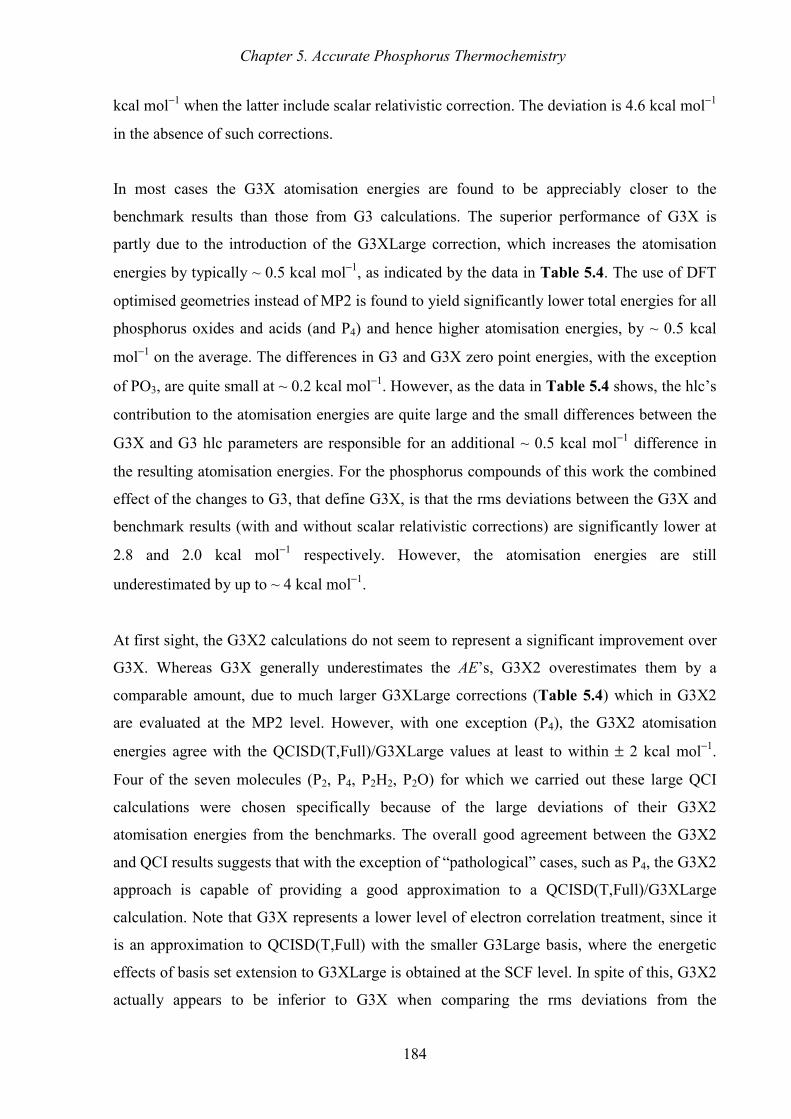
Chapter 5. Accurate Phosphorus Thermochemistry
184
kcal mol−1 when the latter include scalar relativistic correction. The deviation is 4.6 kcal mol−1
in the absence of such corrections.
In most cases the G3X atomisation energies are found to be appreciably closer to the
benchmark results than those from G3 calculations. The superior performance of G3X is
partly due to the introduction of the G3XLarge correction, which increases the atomisation
energies by typically ~ 0.5 kcal mol−1, as indicated by the data in Table 5.4. The use of DFT
optimised geometries instead of MP2 is found to yield significantly lower total energies for all
phosphorus oxides and acids (and P4) and hence higher atomisation energies, by ~ 0.5 kcal
mol−1 on the average. The differences in G3 and G3X zero point energies, with the exception
of PO3, are quite small at ~ 0.2 kcal mol−1. However, as the data in Table 5.4 shows, the hlc’s
contribution to the atomisation energies are quite large and the small differences between the
G3X and G3 hlc parameters are responsible for an additional ~ 0.5 kcal mol−1 difference in
the resulting atomisation energies. For the phosphorus compounds of this work the combined
effect of the changes to G3, that define G3X, is that the rms deviations between the G3X and
benchmark results (with and without scalar relativistic corrections) are significantly lower at
2.8 and 2.0 kcal mol−1 respectively. However, the atomisation energies are still
underestimated by up to ~ 4 kcal mol−1.
At first sight, the G3X2 calculations do not seem to represent a significant improvement over
G3X. Whereas G3X generally underestimates the AE’s, G3X2 overestimates them by a
comparable amount, due to much larger G3XLarge corrections (Table 5.4) which in G3X2
are evaluated at the MP2 level. However, with one exception (P4), the G3X2 atomisation
energies agree with the QCISD(T,Full)/G3XLarge values at least to within ± 2 kcal mol−1.
Four of the seven molecules (P2, P4, P2H2, P2O) for which we carried out these large QCI
calculations were chosen specifically because of the large deviations of their G3X2
atomisation energies from the benchmarks. The overall good agreement between the G3X2
and QCI results suggests that with the exception of “pathological” cases, such as P4, the G3X2
approach is capable of providing a good approximation to a QCISD(T,Full)/G3XLarge
calculation. Note that G3X represents a lower level of electron correlation treatment, since it
is an approximation to QCISD(T,Full) with the smaller G3Large basis, where the energetic
effects of basis set extension to G3XLarge is obtained at the SCF level. In spite of this, G3X2
actually appears to be inferior to G3X when comparing the rms deviations from the

Chapter 5. Accurate Phosphorus Thermochemistry
185
Table 5.4 Various components of the G3X and G3X2 atomisation energies at 0K (in kcal
mol−1).
SCFG3XLargecorrection
MP2(Full)G3XLargecorrection
CP(CV)correction of
G3X2G3X hlc
P2 0.2 −4.5 −1.1 −8.3
P4 0.8 13.7 −3.8 16.6
PH 0.0 −0.9 −0.2 −5.2
PH2 0.1 −1.7 −0.3 −6.8
PH3 0.1 −2.4 −0.4 −8.4
P2H2 0.3 −5.2 −1.2 11.1
P2H4 0.3 −5.5 −1.3 13.9
PO a 0.4 −1.8 −0.8 −6.7
PO2 0.7 −3.0 −1.6 −9.3
PO3 1.1 −4.2 −2.3 12.0
P2O 0.6 −6.0 −2.2 11.0
P2O2 1.9 −6.2 −2.2 13.7
HPO 0.4 −2.4 −0.9 −8.3
HPOH 0.5 −2.2 −0.7 −9.5
H2POH 0.5 −2.9 −0.9 11.1
H3PO 0.5 −3.3 −1.1 11.1
HOPO 0.8 −2.8 −1.4 10.9
HOPO2 1.1 −4.2 −2.3 13.6
a Calculated by G3n(RAD) methods.
benchmark. In the case of G3X2 these are 2.9 and 2.6 kcal mol−1 respectively, when the
benchmarks do and do not include scalar relativistic corrections. The apparent inferiority to
G3X is, however, largely due to the inclusion of P4, an extreme outlier, for which G3X2
predicts the atomisation energy to be up to ~ 9 kcal mol−1 higher than the benchmark. For this
molecule the failure of the G3X2 procedure is partly due to a 3 kcal mol−1 overestimation of
the QCISD(T,Full)/G3XLarge atomisation energy, which itself is a further 5 kcal mol−1
higher than the benchmark. For several other molecules, however, due to the fortuitous
cancellation of errors, the G3X2 results agree slightly better with the benchmarks than those
obtained by QCI. P4 is clearly a special case, and as such, it will be the subject of a more

Chapter 5. Accurate Phosphorus Thermochemistry
186
detailed discussion later in this chapter. At this point, however, it is reasonable to re-evaluate
the rms errors when P4 is removed from the test set. These are now 3.6 and 4.5 kcal mol−1 for
G3; 1.8 and 2.7 kcal mol−1 for G3X and 2.1 and 1.7 kcal mol−1 for G3X2, the two sets of
values corresponding to the inclusion and exclusion of scalar relativistic corrections in the
benchmark results respectively. Thus, G3X2 represents a modest improvement upon G3X
theory for this set of molecules, when compared with benchmark values without scalar
relativistic corrections.
As remarked already, a legitimate modification of G3X and G3X2 would be to consider
corrections to the CV component of the atomisation energies for BSSE. The computed
corrections to the G3X2 energies, that is, at the MP2/G3XLarge level of theory, are given in
Table 5.4. They range from −3.8 to −0.2 kcal mol−1 and reduce the rms deviation from the
benchmark values (with and without scalar relativistic corrections) to 1.8 and 2.0 kcal mol−1
respectively. Omitting P4 from the set results in further reductions in the above deviations to
1.5 and 1.8 kcal mol−1. The analogous corrections to G3X are somewhat smaller but as they
are negative their impact would be to degrade the agreement between the G3X and
benchmark values. The introduction of these proposed modifications of course necessitates
changes to the higher level corrections. As the current set of molecules is too small and not
sufficiently representative, no modifications to the hlc are proposed at this stage. Further work
is under way, however, to produce G3X2 atomisation energies for all the molecules in the
G3/99 test set which contain second row atoms. This will allow re-optimisation of the hlc in
the presence of BSSE corrections as well as a fuller investigation of the need (or otherwise) to
correct the G3X2 energies for scalar relativistic effects. With the current (G3X) choice of hlc
the fluctuation in the deviations of both G3X and G3X2 results is such that, in the rms sense,
a comparable level of agreement is achieved with the two sets of benchmark values. It is
possible, however, that re-optimisation of the hlc on the basis of G3X2 data will change this
apparent insensitivity to relativistic corrections as well as the magnitude of the above rms
deviations.
The deviations of the G3X, G3X2 and QCISD(T,Full)/G3XLarge atomisation energies from
the benchmark results (including scalar relativistic corrections) are summarised graphically in
Figure 5.3. It can be clearly seen that in most cases G3X2 is a good approximation to
QCISD(T,Full)/G3XLarge. Where the difference between G3X2 and QCI is largest, both are

Chapter 5. Accurate Phosphorus Thermochemistry
187
seen to show relatively poor agreement with the corresponding benchmark result, although
corrections to the CV components for BSSE (in both G3X2 and QCI) do improve the
agreement. This occurs for P4, as noted above, and also for PPO. Both are somewhat unusual
molecules. Tetrahedral P4, with 60º bond angles, is a very “strained” molecule, while the
bonding in PPO is best described in terms of a P-P+ triple bond and a P+-O− semipolar bond,
as suggested by the results of a Roby-Davidson population analysis60-62. Thus it should not be
too surprising that such molecules would be difficult to describe accurately.
Figure 5.3 Deviations of G3X, G3X2 and QCISD(T,Full)/G3XLarge atomisation energies
from CCSD(T)/CBS benchmark values (with scalar relativistic corrections).
As we expect that, in general, the G3X2 results would have an uncertainty of approximately ±
2 kcal mol−1, it is noteworthy that all the molecules which fall outside this range (P2, P4, P2H2
and PPO) have multiple or strained P-P bonds. As P2H4 (with a P-P single bond) and P2O2
(with two phosphorus atoms but no P-P bond) are both described adequately by G3X2, it
appears that this method could be expected to provide a satisfactory description of molecules
with second row atoms but care should be taken when these atoms have formal multiple
bonds with each other. As remarked earlier, G3X produces atomisation energies that are
consistently lower than the benchmark values, while in most cases the G3X2 results are on the
-6.0
-4.0
-2.0
0.0
2.0
4.0
6.0
8.0
10.0
Devi
atio
n /
kcal m
ol -1
G3X
G3X2
G3X2 + CP
QCISD(T)
P2
P4
PH
PH2
PH3
P2H2
P2H4
PO
PO2
PO3
P2O
P2O2 HPOH
H2POH
H3PO
HOPO
HPO
HOPO2

Chapter 5. Accurate Phosphorus Thermochemistry
188
high side. There is only one molecule, HOPO2, for which the G3X2 atomisation energy is
significantly below the benchmark result; however, as noted in the previous section, the latter
may be 0.85 kcal mol−1 too high due to the absence of the CCSD(T)/(aug-)cc-pV5Z+d energy
in extrapolations.
5.3.2.1 Analysis of Molecules for Which G3n Methods Perform Poorly
5.3.2.1.1 P4
As noted above, in the case of P4 there is significant deviation between the G3X2 atomisation
energies and those resulting from QCISD(T,Full)/G3XLarge calculations. The discrepancy
suggests at least a partial failure of the underlying assumption of G3 type theories for P4; that
is, that as the basis set is extended, the increased degree of correlation can be adequately
approximated by lower levels of theory than QCISD(T). In order to identify the actual source
of this problem, the individual G3X and G3X2 corrections, namely (+), (2df,p), G3Large,
G3XLarge and G3X2, as defined in Equations (5.5) to (5.8), computed using MP4, MP2 (and
SCF in the case of G3XLarge), are compared with the corresponding corrections evaluated by
QCISD(T). The results for the phosphorus atom and P4 are given in Table 5.5. In the case of
P, the agreement between the corrections obtained by QCISD(T) and the relevant lower levels
of theory is clearly very good, as may be expected. The largest discrepancy is 0.7 kcal mol−1
(in the MP2 determination of the G3Large correction) but in the case of G3X2 this is largely
cancelled by the negative discrepancy in the G3XLarge term. Somewhat fortuitously, thus,
G3X2 represents an excellent approximation to the QCI energy in the case of P. The situation
is quite different for P4, where MP4 overestimates the magnitude of the (2df,p) correction by
3.6 kcal mol−1. The trends and deviations in the other corrections, specifically the G3Large
and G3XLarge corrections, are similar to those observed for the phosphorus atom, provided
we allow for the presence of four atoms in the molecule. Therefore, the major deviation
between the G3X2 and QCI atomisation energies of P4 results from the poor performance of
MP4 in the prediction of the (2df,p) correction, as shown by the analysis of the atomisation
energy in Table 5.5. The total error in the G3Large and G3XLarge terms as obtained by MP2
is −1.1 kcal mol−1. Thus again there is some fortuitous error cancellation, resulting in a total
discrepancy of 3.0 kcal mol−1 in the G3X2 atomisation energy of P4.

Chapter 5. A
ccurate Phosphorus T
hermochem
istry
189
Table 5.5 Basis set enlargement corrections to total G3X and G3X2 energies of P4 and P and to the atomisation energy of P4 at
various levels of theory (in kcal mol−1).
P4 PContribution to
Atomisation Energy
Correction Level of TheoryAbsolutecorrection
Deviation fromQCISD(T) a
Absolutecorrection
Deviation fromQCISD(T) a
Absolutecorrection
Deviation fromQCISD(T) a
+ MP4 −−−4.3 −0.2 −−−0.6 −0.0 −2.0 −−0.2
QCISD(T) −−−4.1 −−−0.6 −1.8
2df,p MP4 −118.8 −3.6 −−16.3 −0.1 53.5 −−3.8
QCISD(T) −115.2 −−16.4 49.7
G3Large MP2(Full) −797.6 −3.6 −198.3 −0.7 −4.4 −−0.7
MP4(Full) −803.3 −2.1 −199.1 −0.0 −7.0 −−1.9
QCISD(T,Full) −801.2 −199.0 −5.1
G3XLarge SCF −−−0.8 18.4 −−−0.0 −1.3 −0.8 −13.2
MP2(Full) −−20.8 −1.6 −−−1.8 −0.5 13.7 −−0.4
MP4(Full) −−20.0 −0.8 −−−1.3 −0.0 14.9 −−0.9
QCISD(T,Full) −−19.2 −−−1.3 14.0
G3X2 MP2(Full) −818.4 2.0 −200.1 −0.2 18.1 −−1.1
MP4(Full) −823.3 −2.9 −200.3 −0.0 21.9 −−2.8
QCISD(T,Full) −820.5 −200.3 19.2
a QCISD(T,Full) for G3Large, G3XLarge and G3X2.
189

Chapter 5. Accurate Phosphorus Thermochemistry
190
5.3.2.1.2 P2O, P2, P2H2
Analysis of G3X and G3X2 results, as applied to P4, was also carried out for P2O, P2, P2H2
and HOPO. The various corrections to the atomisation energies and their deviation from the
QCI values for these four molecules, as well as P4 for ready comparison, are listed in Table
5.6. We recall that for P4 and PPO significant discrepancy in the G3X2 atomisation energy
has been noted in comparison with QCISD(T,Full)/G3XLarge while in the case of P2 and
P2H2 there were no major discrepancies however the results were in poor agreement with the
benchmark calculations. In contrast to these species, good agreement was found between the
G3X2, QCISD(T) and CCSD(T)/CBS results for HOPO. For this set of molecules, the (+)
correction is found to be consistently the smallest (less than 5 kcal mol−1 but becoming larger
as oxygen atoms are added); deviations of MP4 from QCI are found to be small (< 1 kcal
mol−1) and positive. The (2df,p) correction, on the other hand, is by far the largest (up to about
50 kcal mol−1 for P4). The deviations between the MP4 and QCI corrections are again found
to be small and positive for P2, P2H2 and HOPO; for PPO the deviation is also small although
negative, but for P4, as mentioned earlier, it is significantly larger at +3.8 kcal mol−1. The
G3Large, G3XLarge and G3X2 corrections are of intermediate magnitude (4 - 10 kcal mol−1
for G3Large, 3 - 15 kcal mol−1 for correlated G3XLarge corrections and 10 - 20 kcal mol−1 for
G3X2). We note that in general the MP2 results show slightly better agreement with
QCISD(T) (0.5 - 1.5 kcal mol−1 deviation for G3X2) than MP4 (1.0 - 2.8 kcal mol−1). In
addition, the correction terms obtained by MP2 are slightly lower than at the QCI level
(giving a negative deviation), whereas the MP4 differences are all positive. This leads to
significant cancellation of errors when the (+) and (2df,p) (obtained by MP4) and G3X2 (by
MP2) corrections are added, resulting in good agreement between the final QCISD(T) and
G3X2 atomisation energies for P2, P2H2 and HOPO. As noted above, in the case of P4, the
(2df,p) correction is too large to be compensated for by the G3X2 correction, while for PPO
all errors, with the exception of that in the (+) term, tend to reinforce each other, leading to the
observed lack of agreement between G3X2 and QCISD(T,Full)/G3XLarge.

Chapter 5. A
ccurate Phosphorus T
hermochem
istry
191
Table 5.6 Basis set enlargement corrections to the atomisation energies of P4, P2O, P2, P2H2 and HOPO evaluated at various levels of theory
(in kcal mol−1).
P4 P2O P2
Correction Level of Theory CorrectionDeviation from
QCISD(T) aCorrection
Deviation fromQCISD(T) a
CorrectionDeviation from
QCISD(T) a
+ MP4 2.0 0.2 3.2 0.1 0.6 0.1
QCISD(T) 1.8 3.1 0.5
2df,p MP4 53.5 3.8 29.9 −0.5 13.0 0.3
QCISD(T) 49.7 30.3 12.7
G3Large MP2(Full) 4.4 −0.7 6.9 −1.1 4.4 −0.4
MP4(Full) 7.0 1.9 9.4 1.4 5.7 0.9
QCISD(T,Full) 5.1 8.0 4.8
G3XLarge SCF 0.8 −13.2 0.6 −5.8 0.2 −4.3
MP2(Full) 13.7 −0.4 6.0 −0.4 4.5 −0.1
MP4(Full) 14.9 0.9 6.8 0.4 4.8 0.3
QCISD(T,Full) 14.0 6.4 4.5
G3X2 MP2(Full) 18.1 −1.1 12.9 −1.4 8.9 −0.5
MP4(Full) 21.9 2.8 16.2 1.9 10.5 1.2
QCISD(T,Full) 19.2 14.3 9.4
191

Chapter 5. A
ccurate Phosphorus T
hermochem
istry
192
Table 5.6. continued
P2H2 HOPO
Correction Level of Theory CorrectionDeviation from
QCISD(T) aCorrection
Deviation fromQCISD(T) a
+ MP4 0.8 0.1 4.3 0.9
QCISD(T) 0.8 3.4
2df,p MP4 28.6 0.6 32.7 0.6
QCISD(T) 27.9 32.1
G3Large MP2(Full) 5.0 −0.9 8.5 −0.8
MP4(Full) 6.5 0.6 10.3 1.0
QCISD(T,Full) 5.9 9.3
G3XLarge SCF 0.3 −5.3 0.8 −2.4
MP2(Full) 5.2 −0.4 2.8 −0.4
MP4(Full) 5.8 0.3 3.4 0.2
QCISD(T,Full) 5.6 3.2
G3X2 MP2(Full) 10.2 −1.3 11.3 −1.2
MP4(Full) 12.4 0.9 13.7 1.1
QCISD(T,Full) 11.5 12.5
a QCISD(T,Full) for G3Large, G3XLarge and G3X2.
192

Chapter 5. Accurate Phosphorus Thermochemistry
193
5.3.3 Enthalpies of Formation
The heats of formation (at 0 and 298 K) of the molecules studied in this work, generated from
the computed atomisation energies (Table 5.3), are listed Table 5.7, along with experimental
and theoretical values from the chemical literature for comparison. For a number of molecules
there has been an absence of experimental and/or theoretical values; for these the current
calculations provide reliable heats of formation. For several others, where the imprecision in
the literature values is quite large, we are able to offer improved data. It is gratifying,
however, that in all cases the benchmark results agree with the accepted literature values
within the respective error margins, even for P4.
The information in Table 5.7 also allows one to assess the performance of the G3, G3X and
G3X2 methods in the context of thermochemistry. For most molecules, given the large
experimental errors, there appears to be reasonable agreement between the available
experimental heats of formation and those from any of the G3, G3X or G3X2 calculations,
with the obvious exception of P4. The differences are more evident if the comparisons are
made with the benchmark values, in which case the G3X and G3X2 results are clearly
superior to those of G3. As discussed already in the context of AE’s, in general G3X2 appears
to be more accurate than G3X, especially if corrections for BSSE in the CV contributions are
included in the calculations.

Chapter 5. A
ccurate Phosphorus T
hermochem
istry
194
Table 5.7 Enthalpies of formation at 0 and 298K (in kcal mol−1).
Heat of Formation (0K) Heat of Formation (298K)
CCSD(T)CBS a
G3 G3X G3X2G3X2
+ CP(CV)QCI b
CCSD(T)CBS a
G3 G3X G3X2G3X2
+ CP(CV)QCI b Literature c
P2 34.8 35.9 34.7 30.5 31.6 30.4 34.4 ± 1.0 35.5 34.3 30.0 31.2 29.9 34.3 ± 0.5 d
P4 13.9 20.0 18.0 5.1 8.9 8.1 12.1 ± 2.5 18.2 16.2 3.4 7.2 6.4 14.1 ± 0.05 d
PH 56.8 56.2 55.9 55.1 55.2 56.6 ± 1.0 56.0 55.7 54.9 55.0 60.6 ± 8.0 e
57.4 ± 0.6 f
PH2 32.4 33.5 33.1 31.5 31.8 31.5 ± 1.0 32.6 32.2 30.6 30.8 26 ± 23 g
33.1 ± 0.6 f
PH3 2.8 5.0 4.3 2.1 2.5 0.9 ± 1.0 3.1 2.4 0.2 0.6 1.3 ± 0.4 d
P2H2 30.0 32.6 31.4 26.5 27.7 25.9 28.1 ± 1.5 30.6 29.4 24.6 25.8 23.9
P2H4 8.2 13.1 11.6 6.4 7.7 4.9 ± 2.0 9.8 8.3 3.1 4.4 5.0 ± 1.0 h
PO i −7.4 −6.9 −7.5 −8.8 −8.0 −7.6 ± 1.0 −7.1 −7.7 −9.0 −8.2 −5.6 ± 1.0 d
−6.8 ± 1.9 j
−7.8 k
PO2 −69.0 −66.8 −68.5 −70.7 −69.1 −69.7 ± 1.5 −67.5 −69.2 −71.5 −69.9 −66.2 ± 3 j
−70.3 k
PO3 −106.7 −100.2 −105.3 −108.5 −106.2 −107.7 ± 2.0 −101.7 −106.3 −109.5 −107.2 −107.5 k
P2O 2.4 6.2 4.0 −1.4 0.9 −3.1 1.6 ± 1.5 5.5 3.3 −2.1 0.1 −3.9
P2O2 −63.4 −58.5 −61.7 −66.0 −63.8 −65.1 ± 2.5 −59.8 −63.4 −67.7 −65.5
194

Chapter 5. A
ccurate Phosphorus T
hermochem
istry
195
Table 5.7 continued
Heat of Formation (0K) Heat of Formation (298K)
CCSD(T)CBS a
G3 G3X G3X2G3X2
+ CP(CV)QCI b
CCSD(T)CBS a
G3 G3X G3X2G3X2
+ CP(CV)QCI b Literature c
HPO −21.5 −19.6 −21.1 −23.1 −22.2 −22.4 ± 1.0 −20.5 −22.0 −24.0 −23.1 −22.6 k
HPOH −22.7 −20.9 −21.7 −23.4 −22.7 −24.4 ± 1.5 −22.5 −23.4 −25.1 −24.4
H2POH −47.7 −44.3 −45.4 −47.8 −46.9 −50.2 ± 1.5 −46.8 −48.0 −50.3 −49.5
H3PO −48.6 −44.1 −45.7 −48.5 −47.4 −51.5 ± 1.5 −46.9 −48.6 −51.4 −50.2
HOPO −110.4 −106.7 −108.7 −110.7 −109.7 −110.4 −112.0 ± 1.5 −108.3 −110.3 −112.3 −111.3 −112.0 −110.6 ± 3 l
−112.4 k
HOPO2 −168.3 −162.5 −165.1 −168.2 −165.9 −170.6 ± 2.0 −164.8 −167.4 −170.5 −168.1 −168.8 ± 4 l
−171.4 k
a Including scalar relativistic corrections.b QCISD(T,Full)/G3XLarge calculation including G3X higher level correction.c Experimental values unless otherwise indicated by italics and footnotes.d Ref. 63.e Semiempirical estimate, Ref. 63.f Ref. 64.
g Estimate, Ref. 63.h Ref. 65.i Calculated by G3n(RAD) methods.j Ref. 66.k RCCSD(T)/CBS computations, Ref. 15.l Ref. 67.
195

Chapter 5. Accurate Phosphorus Thermochemistry
196
5.4 Conclusion
Using the (R)CCSD(T) quantum chemical method in conjunction with correlation consistent
basis sets, accurate heats of formation have been obtained for a series of small phosphorus
containing molecules. These are regarded as convenient and useful benchmark values,
especially in light of the paucity of accurate experimental values. The computed atomisation
energies and hence heats of formation include complete basis estimates of valence correlation
contributions, core-valence contributions which are corrected for basis set superposition and
scalar relativistic corrections. The equilibrium geometries and vibrational frequencies were
obtained by density functional theory. The resulting benchmark heats of formation are in good
agreement with the available experimental and other high level quantum chemical data.
Utilising the calculated benchmark values, we were able to carry out a critical study of the
accuracy and reliability of three G3n type procedures, G3, G3X and G3X2, for phosphorus
containing molecules. We have found that in general the G3X and G3X2 results are of
comparable accuracy, both reproducing the benchmark heats of formation, on the average, to
within ± 2 kcal mol−1. The relative accuracy of G3X2 improves, however, on the introduction
of BSSE corrections to the core-valence correlation contributions. The problem cases for the
G3n methods appear to be molecules with unusual P-P bonding, such as P2 and P4. 63 64-66 67

Chapter 5. Accurate Phosphorus Thermochemistry
197
5.5 References
1. A. Twarowski, Combustion and Flame, 1993, 94, 91.
2. A. Twarowski, Combustion and Flame, 1993, 94, 341.
3. A. Twarowski, Combustion and Flame, 1995, 102, 41.
4. A. Twarowski, Combustion and Flame, 1996, 105, 407.
5. O. P. Korobeinichev, S. B. Ilyin, T. A. Bolshova, V. M. Shvartsberg and A. A.
Chernov, Combustion and Flame, 2000, 121, 593.
6. O. P. Korobeinichev, T. A. Bolshova, V. M. Shvartsberg and A. A. Chernov,
Combustion and Flame, 2001, 125, 744.
7. M. A. MacDonald, F. C. Gouldin and E. M. Fisher, Combustion and Flame, 2001,
124, 668.
8. K. Sendt and G. B. Bacskay, J. Chem. Phys., 2000, 112, 2227.
9. D. A. Dixon and D. Feller, J. Phys. Chem. A, 1998, 102, 8209.
10. D. A. Dixon, D. Feller and G. Sandrone, J. Phys. Chem. A, 1999, 103, 4744.
11. J. M. L. Martin, Chem. Phys. Lett., 1996, 259, 669.
12. J. M. L. Martin and P. R. Taylor, J. Chem. Phys., 1997, 106, 8620.
13. J. M. L. Martin, Chem. Phys. Lett., 1999, 310, 271.
14. C. W. Bauschlicher, Jr. and A. Ricca, J. Phys. Chem. A, 1998, 102, 8044.
15. C. W. Bauschlicher, Jr., J. Phys. Chem. A, 1999, 103, 11126.
16. T. Helgaker, W. Klopper, H. Koch and J. Noga, J. Chem. Phys., 1997, 106, 9639.
17. T. Helgaker, P. Jørgensen and J. Olsen, Molecular Electronic-Structure Theory; John
Wiley & Sons, Ltd.: Chichester, 2000, 322.
18. L. A. Curtiss, K. Raghavachari, P. C. Redfern, V. Rassolov and J. A. Pople, J. Chem.
Phys., 1998, 109, 7764.
19. L. A. Curtiss, P. C. Redfern, K. Raghavachari and J. A. Pople, J. Chem. Phys., 2001,
114, 108.
20. N. L. Haworth, G. B. Bacskay and J. C. Mackie, J. Phys. Chem. A, 2002, 106, 1533.
21. A. D. Becke, J. Chem. Phys., 1993, 98, 5648.
22. P. J. Stephens, F. J. Devlin, C. F. Chabalowski and M. J. Frisch, J. Phys. Chem., 1994,
98, 11623.
23. A. D. Becke, Phys. Rev. A, 1988, 38, 3098.
24. C. Lee, W. Yang and R. G. Parr, Phys. Rev. B, 1988, 37, 785.

Chapter 5. Accurate Phosphorus Thermochemistry
198
25. K. Raghavachari, G. W. Trucks, J. A. Pople and M. Head-Gordon, Chem. Phys. Lett.,
1989, 157, 479.
26. C. Hampel, K. A. Peterson and H.-J. Werner, Chem. Phys. Lett., 1992, 190, 1.
27. T. H. Dunning, Jr., J. Chem. Phys., 1989, 90, 1007.
28. R. A. Kendall, T. H. Dunning, Jr. and R. J. Harrison, J. Chem. Phys., 1992, 96, 6796.
29. D. E. Woon and T. H. Dunning, Jr., J. Chem. Phys., 1993, 98, 1358.
30. D. Feller, J. Chem. Phys., 1992, 96, 6104.
31. C. Schwartz, Methods in Computational Physics; Vol. 2; Academic Press: New York,
1963, 241.
32. K. A. Peterson and T. H. Dunning, Jr., J. Chem. Phys., 2002, 117, 10548.
33. S. F. Boys and F. Bernardi, Molec. Phys., 1970, 19, 553.
34. R. D. Cowan and M. Griffin, J. Opt. Soc. Am., 1976, 66, 1010.
35. R. L. Martin, J. Phys. Chem., 1983, 87, 750.
36. K. Andersson, P.-Å. Malmqvist, B. O. Roos, A. J. Sadlej and K. Wolinski, J. Phys.
Chem., 1990, 94, 5483.
37. K. Andersson, P.-Å. Malmqvist and B. O. Roos, J. Chem. Phys., 1992, 96, 1218.
38. B. O. Roos, P. R. Taylor and P. E. M. Siegbahn, Chem. Phys., 1980, 48, 157.
39. B. O. Roos, in Ab initio Methods in Quantum Chemistry II, K. P. Lawley, Ed.;
Advances in Chemical Physics, I. Pigogine and S. A. Rice, Eds.; Vol. LXIX; J. Wiley
& Sons Ltd.: Chichester, UK, 1987, p. 399.
40. J. A. Pople, M. Head-Gordon, D. J. Fox, K. Raghavachari and L. A. Curtiss, J. Chem.
Phys., 1989, 90, 5622.
41. L. A. Curtiss, K. Raghavachari, G. W. Trucks and J. A. Pople, J. Chem. Phys., 1991,
94, 7221.
42. L. A. Curtiss, P. C. Redfern, K. Raghavachari, V. Rassolov and J. A. Pople, J. Chem.
Phys., 1999, 110, 4703.
43. A. G. Baboul, L. A. Curtiss, P. C. Redfern and K. Raghavachari, J. Chem. Phys.,
1999, 110, 7650.
44. L. A. Curtiss, K. Raghavachari, P. C. Redfern and J. A. Pople, J. Chem. Phys., 2000,
112, 1125.
45. L. A. Curtiss, K. Raghavachari, P. C. Redfern, A. G. Baboul and J. A. Pople, Chem.
Phys. Lett., 1999, 314, 101.
46. L. A. Curtiss, P. C. Redfern, K. Raghavachari and J. A. Pople, Chem. Phys. Lett.,
1999, 313, 600.

Chapter 5. Accurate Phosphorus Thermochemistry
199
47. D. J. Henry and L. Radom, in Theoretical Thermochemistry, J. Cioslowski, Ed.;
Kluwer: Dordrecht, 2001.
48. P. M. Mayer, C. J. Parkinson, D. M. Smith and L. Radom, J. Chem. Phys., 1998, 108,
604.
49. C. J. Parkinson, P. M. Mayer and L. Radom, J. Chem. Soc., Perkin Trans. 2, 1999, 11,
2305.
50. M. J. Frisch, G. W. Trucks, H. B. Schlegel, G. E. Scuseria, M. A. Robb, J. R.
Cheeseman, V. G. Zakrzewski, J. A. Montgomery, R. E. Stratmann, J. C. Burant, S.
Dapprich, J. M. Millam, A. D. Daniels, K. N. Kudin, M. C. Strain, O. Farkas, J.
Tomasi, V. Barone, M. Cossi, R. Cammi, B. Mennucci, C. Pomelli, C. Adamo, S.
Clifford, J. Ochterski, G. A. Petersson, P. Y. Ayala, Q. Cui, K. Morokuma, D. K.
Malik, A. D. Rabuk, K. Raghavachari, J. B. Foresman, J. Cioslowski, J. V. Ortiz, B.
B. Stefanov, G. Lui, A. Liashenko, P. Piskorz, I. Komaromi, R. Gomperts, R. L.
Martin, D. J. Fox, T. Keith, M. A. Al-Laham, C. Y. Peng, A. Nanayakkara, C.
Gonzalez, M. Challacombe, P. M. W. Gill, B. G. Johnson, W. Chen, M. W. Wong, J.
L. Andres, M. Head-Gordon, E. S. Replogle and J. A. Pople, Gaussian 98 Revision
A.7, Gaussian, Inc.: Pittsburgh, PA, 1998,
51. P. J. Knowles, C. Hampel and H.-J. Werner, J. Chem. Phys., 1993, 99, 5219.
52. MOLPRO 96.3 is a package of ab initio programs written by H.-J. Werner and P. J.
Knowles with contributions from J. Almlöf, R. D. Amos, M. J. O. Degan, S. T. Elbert,
C. Hampel, W. Meyer, K. Peterson, R. Pitzer, A. J. Stone, P. R. Taylor, R. Lindh, M.
E. Mura, T. Thorsteinsson.
53. ACES II is a program product of the Quantum Theory Project, University of Florida.
Authors: J. F. Stanton, J. Gauss, J. D. Watts, M. Nooijen, N. Oliphant, S. A. Perera, P.
G. Szalay, W. J. Lauderdale, S. R. Gwaltney, S. Beck, A. Balková, D. E. Bernholdt,
K.-K. Baeck, P. Rozyczko, H. Sekino, C. Hober, R. J. Bartlett. Integral packages
included are VMOL (J. Almlöf, P. R. Taylor); VPROPS (P. Taylor); ABACUS (T.
Helgekar, H. J. Aa. Jensen, P. Jørgensen, J. Olsen, P. R. Taylor).
54. K. Andersson, M. R. A. Blomberg, M. P. Fülscher, G. Karlström, R. Lindh, P.-Å.
Malmqvist, P. Neogrády, J. Olsen, B. O. Roos, A. J. Sadlej, M. Schültz, L. Seijo, L.
Serrano-Andrés, P. E. M. Siegbahn and P.-O. Widmark, MOLCAS Version 4, Lund
University: Lund, Sweden, 1997,
55. W. Klopper and L. Radom, Private communication.
56. T. H. Dunning, Jr., K. A. Peterson and A. K. Wilson, J. Chem. Phys., 2001, 114, 9244.

Chapter 5. Accurate Phosphorus Thermochemistry
200
57. B. J. Persson, P. R. Taylor and T. J. Lee, J. Chem. Phys., 1997, 107, 5051.
58. B. J. Persson and P. R. Taylor, to be published.
59. G. S. Kedziora, J. A. Pople, M. A. Ratner, P. C. Redfern and L. A. Curtiss, J. Chem.
Phys., 2001, 115, 718.
60. E. R. Davidson, J. Chem. Phys., 1967, 46, 3320.
61. K. R. Roby, Mol. Phys., 1974, 27, 81.
62. R. Heinzmann and R. Ahlrichs, Theor. Chim. Acta, 1976, 42, 33.
63. M. W. Chase, Jr., J. Phys. Chem. Ref. Data, 1998, Monograph 9, 1.
64. J. Berkowitz and H. Cho, J. Chem. Phys., 1989, 90, 1.
65. S. R. Gunn and L. G. Green, J. Phys. Chem., 1961, 65, 779.
66. J. Drowart, C. E. Myers, R. Szwarc, A. Vander Auwera-Mahieu and O. M. Uy, J.
Chem. Soc., Faraday Trans. 2, 1972, 68, 1749.
67. D. L. Hildenbrand and K. H. Lau, J. Chem. Phys., 1994, 100, 8373.

6 The Role of the NNH +O Reaction in the Production of NO in Flames
Chapter 6
The Role of the
NNH + O Reaction
in the Production of
NO in Flames

Chapter 6: NNH + O in NO Production
202
The work described in this chapter involves a thermochemical and kinetic study of the
importance of the NNH + O reaction in the production of NO in flames. This work comprises
of two halves: the quantum chemical investigation of the potential energy surface (including
the characterisation of all stationary points) followed by the calculation of the rates of all
possible reactions and the kinetic modelling of various flame systems. The latter half of the
work was performed by Associate Professor John Mackie.
6.1 Introduction
The presence of nitric oxide in the atmosphere is largely the consequence of combustion
processes. As a result, many governments have recently placed stringent limits on the levels
of emission of NO from combustion facilities. It is important in the development of new
combustion technology that accurate chemical kinetic models of the combustion process be
developed to predict the concentrations of NO produced.
Nitric oxide is produced in combustion via four main pathways.1 The first of these is the well
known Zel’dovich or thermal route, initiated by the reaction
2N + O N + NO (6.1)
The prompt-NO route is initiated by
2CH + N HCN + N (6.2)
A third route involves the formation of the intermediate, N2O, and, for fuels containing fuel-
bound nitrogen, there is a fuel-NO route.
Recently, Bozzelli and Dean2 have discovered an additional pathway involving the
intermediate NNH radical, formed by the reaction of H with molecular nitrogen:
2N + H NNH (6.3)

Chapter 6: NNH + O in NO Production
203
The subsequent reaction of NNH with atomic oxygen then yields the products NO and NH:
NNH + O NO + NH→ (6.4)
Using the QRRK technique, Bozzelli and Dean2 estimated the rate coefficient for this reaction
to be 134 7 10k = × cm3 mol−1 s−1 at 2000 K. This reaction and its rate coefficient have been
subsequently incorporated into detailed chemical kinetic reaction models such as GRIMech
2.113 and its successor, GRIMech 3.04, developed to predict species profiles in the
combustion of C1 and C2 hydrocarbons.
There have been no direct experimental studies of the reactions of NNH + O → products. In a
study of NO profiles in laminar premixed flames of H2 / O2 / N2, however, Hayhurst and
Hutchinson5 observed enhanced production rates of NO in the burnt gases that could not be
explained on the basis of the Zel’dovich mechanism alone. They attributed their faster
observed rates to the operation of the NNH + O pathway and, from a steady state analysis of
their experimental NO profiles, arrived at a value of 4 ,3Pk K = ( )91.4 10 exp 2760 T× − cm3
mol−1 s−1 over the temperature range of 1800 – 2500 K; here 4k is the rate coefficient of
Reaction (6.4) and ,3PK is the equilibrium constant of Reaction (6.3). From estimates of the
NNH thermochemistry, they evaluated the equilibrium constant and arrived at a value of
144 1 10k = × cm3 mol−1 s−1, constant within a factor of 2.5, over the temperature range of 1800
– 2500 K. This result is comparable with the rate coefficient originally estimated by Bozzelli
and Dean2.
Recently, experimental and modelling studies of NO profiles in premixed flames6 and in
completely stirred reactors7 have concluded, however, that in circumstances where the NNH +
O route is likely to be important (that is, where the thermal and prompt NO routes are
unimportant), models which employ the above rate coefficient for Reaction (6.4) lead to
overprediction of NO production.
The current study is therefore motivated to make a detailed investigation of the NNH + O
reaction potential energy surface using current techniques of computational quantum
chemistry. Such a study will allow the calculation of reliable thermochemical and kinetic data

Chapter 6: NNH + O in NO Production
204
which can subsequently be applied to the modelling of combustion reactions in the presence
of nitrogen.
Following Bozzelli and Dean, we have included
2NNH + O N O + H→ (6.5)
and
2NNH + O N + OH→ (6.6)
in our system of reactions (in addition to Reactions (6.3) and (6.4)) as potentially competing
channels to the production of NO in Reaction (6.4).
Reactions (6.4) to (6.6) are expected to take place via a common ONNH intermediate, which
decomposes to yield NO + NH, N2O + H or N2 + OH. While no studies of the O + NNH
association have previously been reported, the three decomposition reactions have been
extensively investigated in the chemical literature over the past 18 years8-17. It has been found
that ONNH, a planar molecule, is stable in both cis and trans forms. Although the latter is
generally predicted to be the more stable10-13, it has been concluded that decomposition to
N2O + H and N2 + OH actually occurs via the cis isomer.12,13
Several other reactions are also considered in this work, in particular
NNH O products+ → → (6.7)
where the intermediate, ONHN, is an isomer of ONNH which can yield HNO + N, N2O + H
and N2 + OH as decomposition products.
N
N
HO

Chapter 6: NNH + O in NO Production
205
The isomerisation reactions between cis- and trans-ONNH and between trans-ONNH and
ONHN are alternative channels which have also been studied, along with the direct
abstraction reaction
2NNH O N OH+ → + (6.8)
The stability of the NNH intermediate plays a crucial role in determining the relative
importance of channels (6.4), (6.5) and (6.6) in the chemistry of nitrogen in flames, in
particular the reaction flux which passes through channel (6.4) to generate NO. High level
quantum chemical calculations by Walch and Partridge18 and by Gu et al.19 have predicted the
exothermicity of Reaction (6.3) to be between 3.8 and 4.3 kcal mol−1, with a barrier height of
10.0 - 11.3 kcal mol−1. As modelling studies are extremely sensitive to the stability of NNH,
in the present work we have also undertaken the computation of the heats of formation of both
NNH and the transition state leading to its formation (NN-H) at the highest currently
achievable level of theory available to us, viz. complete basis estimates of the CCSD(T)
(coupled cluster theory with single, double and perturbative triple excitations) energetics
based on extrapolation of aug-cc-pVxZ results with x = 5, 6.
This work therefore involves an extensive investigation of the N2OH potential energy surface
using high level quantum chemical methods followed by the computation of the rate
parameters for all NNH + O → products channels. Finally, in conjunction with the data set of
the GRIMech 3.0 model, we use our revised thermochemistry and rate data to model the lean
combustion of CO / H2 / air and CH4 / air in completely stirred reactors.
6.2 Theory and Computational Methods
6.2.1 Quantum Chemical Calculations of Thermochemistry
Heats of formation and other thermochemical data were computed via two different
approaches: the Gaussian-3X (G3X) method of Curtiss et al.20 and a CCSD(T)/CBS type
scheme, utilising coupled cluster theory with single, double and (perturbative) triple
excitations (CCSD(T)21,22) in conjunction with the correlation consistent basis sets23-25, aug-

Chapter 6: NNH + O in NO Production
206
cc-pVQZ and aug-cc-pV5Z, and extrapolation to the hypothetical complete basis set (CBS)
limit.
In both schemes molecular geometries and vibrational frequencies for equilibrium structures
and transition states were determined by Density Functional Theory (DFT), using the B3LYP
hybrid density functional26-28 with the 6-31G(2df,p) basis set (frequencies scaled by 0.9854).
Single point energy calculations were then performed at these geometries as required for the
two different methodologies, viz. G3X and CCSD(T)/CBS. Open shell systems were treated
by unrestricted calculations in the DFT geometry optimisations (UB3LYP) and the
subsequent implementation of G3X but by restricted, RCCSD(T), methods in the
CCSD(T)/CBS computations.
In the case of the CCSD(T)/CBS{Q,5} scheme, the single point energies were extrapolated to
the complete basis limit using the 3x− extrapolation29
( ) 3E x A Bx−= + (6.9)
where x = 4, 5. In the case of a few species, e.g. NNH, more extensive calculations were
performed where the sequence of basis sets include aug-cc-pV6Z, viz. x = 6. Core-core and
core-valence correlation (CV) corrections were evaluated at the CCSD(T)/aug-cc-pCVQZ
level of theory. Scalar relativistic effects (Darwin and mass-velocity terms)30,31 were
determined by complete active space SCF (CASSCF)32,33 theory using cc-pVTZ basis sets.
Spin-orbit corrections were also included for atomic species.34
As several important reactions, including the formation of ONNH and its decomposition to
NO + NH, are barrierless, Variational Transition State Theory (VTST)35-37 was utilised to
locate and characterise the transition states at a range of temperatures between 1000 and 2500
K. As in previous work of ours38, density functional theory (B3LYP/6-31G(2df,p)) was used
to map the minimum energy path (MEP) along the potential energy surface (PES) as a
function of the reaction coordinate. The latter was approximated as the critical bond forming
or bond breaking distance; thus this critical bond distance was systematically varied while all
other geometric parameters were allowed to relax. At each such point along the reaction
coordinate the rate coefficient was calculated by the application of the canonical transition

Chapter 6: NNH + O in NO Production
207
state formula39 at the given temperature, thus allowing the geometry which yielded the
minimum rate to be identified as the variational transition state.
The Gaussian 98 programs40 were used to perform all DFT calculations (geometry
optimisations and PES scans) as well as the G3X calculations, while MOLPRO21,41,42 was
utilised for all (R)CCSD(T) computations. The CASSCF calculations of scalar relativistic
corrections were carried out using DALTON43 for all molecules and MOLCAS44 for atomic
species. The computations were performed on DEC alpha 600/5/333 and COMPAQ
XP100/500 workstations of the Theoretical Chemistry group at the University of Sydney and
on the COMPAQ AlphaServer SC system of the Australian Partnership for Advanced
Computing National Facility at the National Supercomputing Centre, ANU, Canberra.
6.2.2 Derivation of Rate Coefficients for Individual Reaction
Channels
As discussed above, addition of O to NNH produces three intermediates via chemical
activation. These intermediates, which represent local minima on the potential energy surface,
are trans-ONNH, cis-ONNH and ONHN. Further reaction leads to four product channels, that
is, to NO + NH, N2O + H, N2 + OH and HNO + N. All but the last of these are exothermic
processes. To derive rate coefficients for the overall reaction to the four product channels we
have separately considered the three reaction surfaces for
NNH + O ONNH productstrans - → (6.10)
NNH + O ONNH productscis - → (6.11)
and
NNH + O ONHN products→ (6.12)
We then assume that the vibrationally excited adduct (trans-ONNH, cis-ONNH or ONHN), is
formed from NNH and O at an energy, E, and will undergo the reverse reaction at an energy-

Chapter 6: NNH + O in NO Production
208
specific rate coefficient, ( )k E . The limiting high-pressure rate coefficient for this reverse
(dissociation) reaction, ,unik ∞ , is given by
0,
1( ) ( ) exp( / )
( )uni BEk k E E E k T dE
q Tρ
∞
∞ = −∫ (6.13)
where ( )q T is the internal partition function of the adduct calculated at the translational
temperature, T; ( )Eρ is the density of states and Bk is Boltzmann’s constant. The lower limit
for integration is the critical energy of reaction, 0E . The recombination rate coefficient in the
high pressure limit, ,reck ∞ , is obtained from ,unik ∞ by detailed balance using the equilibrium
constant ( )cK T as given by
( ),
,uni
recc
kk
K T∞
∞ = (6.14)
The overall pressure-dependent rate coefficient via each adduct to each of the product
channels is obtained from
,overall products reck f k ∞= × (6.15)
where prodsf is the fraction of reaction flux to each product channel. We have carried out an
RRKM analysis using the MultiWell suite of programs developed by Barker45 to solve the
internal master equation with densities of states calculated by an exact count method.
Collisional energy transfer parameters were taken from the work of Barker.46 Lennard-Jones
parameters have been taken from the Chemkin Collection.47 As all three adducts lead to the
four reaction channels (but with different values of productsf ), the final overall rate coefficients
for NNH + O → products were obtained by summing the contributions from the three
surfaces.
Chapter 6: NNH + O in NO Production
209
6.3 Results and Discussion
6.3.1 Quantum Chemistry
All potential stationary points on the NNH + O PES were investigated using B3LYP/
6-31G(2df,p) on both the A′ and A″ surfaces. The A′ species were found to be consistently
lower in energy (as found by other workers), so in general only results for this surface are
presented.
The electronic energies of the stationary points on the PES as calculated at the (valence
correlated) CCSD(T)/aug-cc-pVQZ and CCSD(T)/aug-cc-pV5Z levels of theory, along with
the extrapolated results, are presented in Table 6.1. This Table also provides details of the
CCSD(T)/aug-cc-pCVQZ core-valence correlation corrections, the scalar relativistic
corrections and the zero point energies for each molecule, and thus the total CCSD(T)/CBS
energy at 0K together with the corresponding G3X result. The thermal corrections between 0
and 298K for each molecule are also reported here. Unfortunately, it was not possible to
perform such CCSD(T)/CBS calculation on the cis to trans transition state of ONNH (ONNH
c-t TS), as the lack of symmetry in this molecule made the aug-cc-pV5Z and aug-cc-pCVQZ
calculations too large. The geometries, rotational constants and vibrational frequencies for all
equilibrium structures, transition states and variational transition states are summarised in
Appendix 3 (schematic structures for these species can also be found in Figures 6.1 to 6.3).
Table 6.2, in turn, contains the atomisation energies for each species as calculated using both
the CCSD(T)/CBS and G3X approaches, as well as the resulting heats of formation at 0 and
298 K and literature values for the latter where available. Core-valence correlation and
relativistic contributions to the atomisation energies are also included in this Table.
Examination of the latter reveals that both effects are relatively small in magnitude and that
their respective contributions cancel out to a large extent, resulting in a net contribution of
~ 0.5 kcal mol−1 or less.
According to Curtiss et al.20, the heats of formation obtained from the G3X method are
expected to have a mean absolute deviation of 1.0 kcal mol−1 from experiment. The
CCSD(T)/CBS results are expected to have a higher degree of accuracy; our conservative

Chapter 6: N
NH
+ O
in NO
Production
210
Table 6.1 Total CCSD(T) and G3X energies, core-valence (CV) correlation corrections, scalar relativistic corrections (in hE ) along with zero
point energies and thermal corrections to enthalpies (in kcal mol−1).
Valence correlated energy CV corr relE∆ ZPE Total Energyb 0 0298 0H H−
CCSD(T) CCSD(T) CCSD(T) CCSD(T) CASSCF B3LYP CCSD(T) B3LYP
aug-cc-pVQZ aug-cc-pV5Z CBS{Q,5}a aug-cc-pCVQZ cc-pVTZ 6-31G(2df,p) CBS{Q,5}G3X
6-31G(2df,p)
N 4S −54.52506 −54.52780 −54.53068 −0.05613 −0.02921 −54.61601 −54.56490 1.04
O 3P −74.99493 −75.00041 −75.00615 −0.05907 −0.05237 −75.11795 −75.03224 1.04
H 2S −0.49995 −0.49999 −0.50004 0.00000 0.00000 −0.50004 −0.50097 1.01
N2 1Σg −109.40724 −109.41551 −109.42418 −0.11344 −0.05818 3.42 −109.59034 −109.48808 2.07
NH 3Σ −55.15574 −55.15913 −55.16269 −0.05628 −0.02906 4.57 −55.24075 −55.19350 2.07
NO 2Π −129.75792 −129.76818 −129.77893 −0.11585 −0.08085 2.80 −129.97117 −129.83624 2.07
OH 2Π −75.66426 −75.67038 −75.67680 −0.05929 −0.05187 5.21 −75.77967 −75.69607 2.07
NNH 2A′ −109.90091 −109.90907 −109.91763 −0.11344 −0.05790 8.18 −110.07595 −109.97501 2.39
NNO 1Σ −184.46683 −184.48141 −184.49671 −0.17313 −0.10956 6.98 −184.76828 −184.58323 2.27
HNO 1A′ −130.34240 −130.35288 −130.36388 −0.11587 −0.08067 8.54 −130.54681 −130.41227 2.37
trans-ONNH 2A′ −185.00994 −185.02643 −185.04373 −0.17290 −0.10949 13.04 −185.30534 −185.11715 2.52
cis-ONNH 2A′ −185.00041 −185.01644 −185.03325 −0.17297 −0.10948 12.56 −185.29569 −185.10725 2.56
ONHN 2A′ −184.97089 −184.98820 −185.00636 −0.17270 −0.10952 12.52 −185.26863 −185.07844 2.53
NN-H 2A′ −109.88513 −109.89336 −109.90200 −0.11332 −0.05813 4.05 −110.06699 −109.96623 2.46
ONN-H 2A′ −184.95143 −184.96843 −184.98626 −0.17301 −0.10955 7.38 −185.25707 −185.06898 2.76
ON2-H 2A′ −184.92953 −184.94647 −184.96424 −0.17276 −0.10957 7.77 −185.23418 −185.04605 2.57
NNOHsq 2A′ −184.94179 −184.95694 −184.97283 −0.17210 −0.10985 8.91 −185.24059 −185.05381 2.50
NNOHtr 2A′ −184.92091 −184.93646 −184.95278 −0.17257 −0.10976 8.20 −185.22205 −185.03713 2.71
ONNH c-t TS 2A −185.08082
ONHN-ONNHt 2A′ −184.91787 −184.93264 −184.94813 −0.17260 −0.10956 9.02 −185.21592 −185.03186 2.63
a Extrapolated CCSD(T) energy to CBS (x = ∞) limit using x = 4, 5 data. b Including CV, rel
E∆ and ZPE corrections in CCSD(T)/CBS energies.

Chapter 6: N
NH
+ O
in NO
Production
211
Table 6.2 CCSD(T)/CBS{Q,5} and G3X atomisation energies (along with CV correlation and scalar relativistic contributions to CBS) and
heats of formation (at 0 and 298K) of reactants, products, intermediates and first order saddle points on the N2OH surface (in kcal mol−1).
Atomisation Energya 00f H∆ 0
298f H∆
CV corr relE∆ CCSD(T)b
CBSG3X
CCSD(T) b
CBSG3X
CCSD(T) b
CBSG3X Experiment
N2 0.74 −0.15 224.9 224.8 0.2 0.2 0.2 0.2 0.00
NH 0.09 −0.09 78.3 80.1 85.9 84.1 85.9 84.1 85.32 ± 0.02c
NO 0.41 −0.46 148.9 150.0 22.7 21.5 22.7 21.5 21.82 ± 0.04d
OH 0.14 −0.31 101.5 102.2 9.2 8.4 9.2 8.5 8.83 ± 0.09e
NNH 0.74 −0.33 215.8 216.0 60.9 60.7 60.2 60.0
NNO 1.13 −0.77 262.5 264.3 21.6 19.8 20.7 18.9 19.6 ± 0.1f
HNO 0.42 −0.57 196.3 197.1 26.9 26.0 26.2 25.3 25.60.60.1
+−
g
trans-ONNH 0.99 −0.82 285.7 285.0 50.0 50.7 48.4 49.1
cis-ONNH 1.03 −0.82 279.7 278.8 56.0 56.9 54.5 55.4
ONHN 0.86 −0.80 262.7 260.7 73.0 75.0 71.4 73.4
NN-H 0.67 −0.18 210.2 210.5 66.5 66.2 65.9 65.6
ONN-H 1.05 −0.78 255.4 254.8 80.3 80.9 78.9 79.6
ON2-H 0.90 −0.77 241.1 240.4 94.6 95.3 93.1 93.8
NNOHsq 0.48 −0.59 245.1 245.2 90.6 90.5 89.0 88.8
NNOHtr 0.78 −0.65 233.5 234.8 102.2 100.9 100.8 99.5
ONNH c-t TS 262.2 73.5 71.9
ONHN-ONNHt 0.80 −0.77 229.6 231.5 106.1 104.2 104.6 102.7
a Including zero-point corrections.b Including CV correlation and
scalar relativistic corrections.
c 0
0fH∆ from Ref. 48 with thermal corrections
from this work.48
d Ref. 49.49
e Ref. 50.50
f Ref. 49.g Ref. 51.51

Chapter 6: NNH + O in NO Production
212
estimate for the maximum uncertainty in any of the CBS heats of formation computed in this
work is ± 1.0 kcal mol−1. Comparison of the CCSD(T)/CBS and G3X heats of formation
indicates the two sets of results agree with each other and with the available experimental data
within their respective error margins.
In light of the sensitivity of the kinetic models to the stability of NNH, as noted above, a more
extensive investigation was carried out for NNH, N2 and the transition state, NN-H. The
geometries and harmonic frequencies were redetermined at the CCSD(T)/aug-cc-pVQZ level
of theory using numerical differentiation to obtain the appropriate force constants. The
CCSD(T) valence correlated energies were calculated at the revised geometries using the aug-
cc-pV5Z and aug-cc-pV6Z basis sets52,53 and extrapolated as before. CCSD(T)/aug-cc-
pCVQZ CV corrections, CASSCF/cc-pVTZ scalar relativistic corrections and atomic spin
orbit corrections were again applied. In order to account, at least in part, for the effects of
anharmonicity in the calculation of the zero-point energies and thermal corrections, the NNH
bending frequencies were scaled by a factor of 0.97, the N-N stretching frequencies by 0.988
and the N-H stretching frequencies by 0.95. (These scaling factors were chosen by
comparison of experimental harmonic and anharmonic frequencies of N2, NH3 and H2O.) The
results of these high level calculations are summarised in Table 6.3. As can be seen by
comparison with the results in Table 6.2, the application of a substantially higher level of
theoretical treatment leaves the heats of formation for N2 and NNH largely unchanged; it
does, however, reduce the barrier for the dissociation of NNH by ~ 1 kcal mol−1.
Comparison of the CCSD(T)/aug-cc-pV5Z energies at the revised CCSD(T) geometries (in
Table 6.3) with those at B3LYP geometries (in Table 6.1) demonstrates that for N2 and NNH
the small geometric changes (less than 0.01 Å in bond lengths and 0.6° in the NNH bond
angle) have a negligible effect on the energies. For the NN-H transition state, however, the
energy has been lowered by ~ 1 kcal mol−1; this is accompanied by a decrease of 0.12 Å in the
N-H bond length. The zero-point energies are effectively unchanged (differences of ~ 0.1 kcal
mol−1 or less). For N, N2 and NNH the CCSD(T)/CBS{5,6} energies are 0.54, 1.16 and 1.54
kcal mol−1 higher than the corresponding {Q,5} results. Thus, the effects of the extra degree
of theoretical complexity implicit in the aug-cc-pV6Z calculations largely cancel in the
atomisation energy computations of N2 while the value for NNH is reduced by ~ 0.4 kcal
mol−1. Interestingly, for the NN-H transition state the combined effects of geometry changes

Chapter 6: NNH + O in NO Production
213
Table 6.3 Summary of the energetic contributions to the CCSD(T)/CBS{5,6} extrapolated
atomisation energies (AE) and heats of formation for N2, NNH and the NN-H transition state
(in hE unless otherwise noted).
N H N2 NNH NN-H
CCSD(T)/aug-cc-pV5Z −54.52780 −0.49999 −109.41550 −109.90913 −109.89164
CCSD(T)/aug-cc-pV6Z −54.52865 −0.50000 −109.41838 −109.91167 −109.89596
CCSD(T)/CBS{5,6} −54.52982 −0.50001 −109.42233 −109.91517 −109.90200
CCSD(T)/aug-cc-pCVQZ(core + valence) −54.58205 −109.52248 −110.01611 −109.99847
CCSD(T)/aug-cc-pCVQZ(valence only) −54.52592 −109.40906 −109.90267 −109.88515
CV correction −0.05613 −0.11342 −0.11343 −0.11332
relE∆ −0.02921 −0.05818 −0.05790 −0.05811
ZPE 0.00526 0.01287 0.00644
CCSD(T)/CBS {5,6} a −54.61516 −0.50001 −109.58867 −110.07363 −110.06698
CCSD(T)/CBS {5,6} AE a
/kcal mol−1 224.87 215.43 211.26
CCSD(T)/CBS {5,6} 00f H∆ a
/kcal mol−1 0.19 61.26 65.43
0 0298 0H H− /kcal mol−1 1.04 1.01 2.07 2.39 2.44
CCSD(T)/CBS {5,6} 0298f H∆ a
/kcal mol−1 0.18 60.56 64.78
a Including CV, rel
E∆ and ZPE corrections.
and larger basis set have resulted in a CCSD(T)/CBS{5,6} energy that is essentially the same
as that obtained via CCSD(T)/CBS{Q,5}. The net results is therefore a lower atomisation
energy for NN-H; that is, the barrier to dissociation is reduced, by ~ 1 kcal mol−1. These
results are in support of our proposed uncertainty of ± 1 kcal mol−1 in our CCSD(T)/CBS
heats of formation.
In Table 6.4, the G3X and CCSD(T)/CBS energetics are compared with the earlier theoretical
work of Walch12,18, Gu19 and Durant13. As these workers reported their results as energies
relative to N2 + H (for NNH and NN-H) and NO + NH for all other species, we also present

Chapter 6: NNH + O in NO Production
214
Table 6.4 Energiesa of NNH and N2OH species relative to N2 + H and NO + NH respectively
computed at different levels of theory (in kcal mol−1).
CCSD(T)CBS {Q,5}
CCSD(T)CBS {5,6}
G3X G2b MR-CIcCCSD(T)/
aug-cc-pVQZd
MR-CI +Dav.e
NNH 9.1 9.4 8.8 8.6 ± 0.5 9.1
NN-H 14.7 13.6 14.3 14.4 ± 1.0 16.3
trans-ONNH −58.6 −54.9 −56.0 −51.5
cis-ONNH −52.6 −48.6 −48.9 −46.2
ONHN −35.6 −30.6
O + NNH 11.3 14.1
NNO + H −35.4 −34.2 −34.5 −31.7
N2 + OH −99.2 −96.9 −96.9
ONNH c-t TS −32.1 −30.8
ONN-H −28.3 −24.6 −25.3 −21.4
ON2-H −14.0 −10.2
NNOHsq −18.0 −15.1 −17.9 −15.4
NNOHtr −6.4 −4.6
ONHN-ONNHt −2.5 −1.3
a Including zero-point corrections.b Ref. 13.c Ref. 12.d Ref. 19 + B3LYP/6-31G(2df,p) zero point energy.e MR-CI values, including Davidson’s correction, from Ref. 18 + B3LYP/6-31G(2df,p) zero point energy.
our results in this form for easy comparison. Note also that the previous calculations on NNH
and NN-H by Walch and Partridge18 and by Gu, Xie and Schaefer19 reported only electronic
energy differences; we have therefore added our B3LYP/6-31G(2df,p) zero-point energies to
their values for consistency. The results of Gu et al.19 were obtained via CCSD(T)/
aug-cc-pVQZ calculations while Walch and Partridge utilised multireference CI (MRCI)
(including Davidson’s correction) in conjunction with the cc-pVxZ, x = D, T, Q, 5 basis sets
and extrapolation via the exponential formula:
( ) ( )expE x A B Cx= + − (6.16)

Chapter 6: NNH + O in NO Production
215
While there is broad agreement with respect to the stability of NNH, our best estimate of the
barrier height for its dissociation is lower that those obtained by either of the other groups.
Thus our results indicate that NNH is significantly less stable to dissociation and has a shorter
lifetime than previously predicted.
The energies of the N2OH species are compared in Table 6.4 with the G2 values of Durant13
and the MRCI results of Walch12. As may be expected, the G2 and G3X results are, in most
cases, in good agreement. Walch’s MRCI results, however, are found to be consistently
higher than those obtained by either G2, G3X or CCSD(T)/CBS. We believe that this
discrepancy is due to size extensivity problems in the MRCI approach, which in this case did
not include Davidson’s correction. Such problems are expected to be most serious in the
calculation of dissociation energies. Consequently, as noted by Durant13, in Walch’s
calculations the stabilities of the N2OH species (as well as of N2O + H) relative to NO + NH
are underestimated by ~ 3 kcal mol−1; when a correction of this size is applied to the MRCI
results the agreement with the G2 and G3X results is much improved. It is seen, however, that
the CCSD(T)/CBS{Q,5} results are generally significantly lower than their G3X counterparts,
by up to 3.7 kcal mol−1.
We believe that for the systems studied here the CCSD(T)/CBS approach, as outlined in this
work, represents potentially the highest level of size consistent treatment of electron
correlation that is currently available. Consequently, we expect our CCSD(T)/CBS results to
be more accurate than those obtained previously.
6.3.2 Potential Energy Surfaces and Reaction Paths
Schematic potential energy diagrams showing the major stationary points on the N2OH
potential energy surface corresponding to the three main reaction channels (Equations (6.10)
to (6.12)) are shown in Figures 6.1 to 6.3. The relative enthalpies (at 298K) shown in these
diagrams are CCSD(T)/CBS{Q,5} values, except for ONNH c-t TS where the G3X result has
been used. Clearly, the reaction channels producing N2O + H and N2 + OH are
thermodynamically favoured over the formation of NO + NH. On the other hand, the reaction
to form N + HNO is calculated to be endothermic by 19.4 kcal mol−1 and thus unlikely to
compete with the other more favourable channels.

Chapter 6: NNH + O in NO Production
216
-47.9
-65.3
-30.8
-110.4
-11.2
-71.4
-40.9
-46.9
0.00
NNH + O
NO + NH
trans -ONNH
ONN-H
NNO + H
ONNH c -t TS
cis -ONNH
N2 + OH
NNOHsq
Figure 6.1 Schematic of potential energy surfaces for the reactions of trans-ONNH. Relative
enthalpies at 298 K (in kcal mol−1) from CCSD(T)/CBS{Q,5} calculations.
-46.9
-40.9
-65.3
-30.8
-110.4
0.0
-11.2
NNH + O
NO + NH
ONN-H
NNO + H
cis -ONNH
NNOHsq
N2 + OH
Figure 6.2 Schematic of potential energy surfaces for the reactions of cis-ONNH. Relative
enthalpies at 298 K (in kcal mol−1) from CCSD(T)/CBS{Q,5} calculations.
N
H
NO
N N
HO
O
N N
H
O
N N
H
N N
H
O
N
H
NO
N
O
N
HO
N N
H
N N
H
O
N N
H
O
O
N N
H
N N
H
O

Chapter 6: NNH + O in NO Production
217
19.4
-46.9-26.7
-15.20.0
-71.4
-110.4
-18.9
-48.3
NNH + O
trans -ONNH
ONHN
ONHN-ONNHt NNOHtr
N2 + OH
ON2-HNNO + H
HNO + N
Figure 6.3 Schematic of potential energy surfaces for the reactions of ONHN. Relative
enthalpies at 298 K (in kcal mol−1) from CCSD(T)/CBS{Q,5} calculations.
As several of the reactions on this PES involve barrierless recombinations or dissociations,
variational transitions state theory was applied in order to locate and characterise the
(temperature dependent) transition states, as described in the Section 6.2.1. Energies, and thus
heats of formation, at the CCSD(T)/CBS level of theory were estimated by utilising the
B3LYP/6-31G(2df,p) estimate of the energy difference between the TS and the dissociated
adducts along with the CCSD(T)/CBS energies for the dissociated species. The resulting heats
of formation are listed in Table 6.5. Geometries, rotational constants and vibrational
frequencies for these species are given in Appendices 3.3 and 3.4.
N
N
HO
N
O
N
H
N
N
O H
N
N
HO
N
N
O H
O
N
H
N
N
N
O
H

Chapter 6: NNH + O in NO Production
218
Table 6.5 G3X and CCSD(T)/CBS{Q,5} total energies, atomisation energies (at 0K) and
heats of formation (at 0 and 298K) of variational transitions states (in kcal mol−1).
Reaction Temp. /K00f H∆ 0
298f H∆
G3X CBS G3X CBS
trans-ONNH → NNH + O 1000 116.1 116.3 115.1 115.3
1500 114.2 114.5 113.1 113.4
2000 112.1 112.3 110.9 111.1
2500 109.6 109.8 108.3 108.5
cis-ONNH → NNH + O 1000 116.8 117.1 115.9 116.1
1500 116.2 116.4 115.2 115.4
2000 114.9 115.1 113.9 114.1
2500 112.7 112.9 111.5 111.8
ONHN → NNH + O 1000 117.0 117.2 116.1 116.3
1500 115.5 115.7 114.5 114.8
2000 111.4 111.7 110.3 110.5
2200 107.0 107.2 105.7 105.9
trans-ONNH → NO + NH 1000 99.8 102.9 98.9 102.0
1500 98.6 101.6 97.6 100.6
2000 97.1 100.1 96.1 99.1
2400 96.7 99.7 95.6 98.6
cis-ONNH → NO + NH 1000 99.6 102.6 98.7 101.7
1500 98.2 101.3 97.3 100.3
2000 96.7 99.7 95.6 98.6
2500 96.2 99.2 95.1 98.1
ONHN → N + HNO 1000 135.5 136.4 134.2 135.0
1500 135.1 135.9 133.7 134.6
2000 134.5 135.3 133.1 133.9
2500 134.1 135.0 132.7 133.5
NNH + O → N2 + OH 1000 117.8 118.0 116.8 117.0
1500 116.9 117.2 115.8 116.1
2000 115.7 116.0 114.6 114.8
2500 115.3 115.5 114.1 114.3
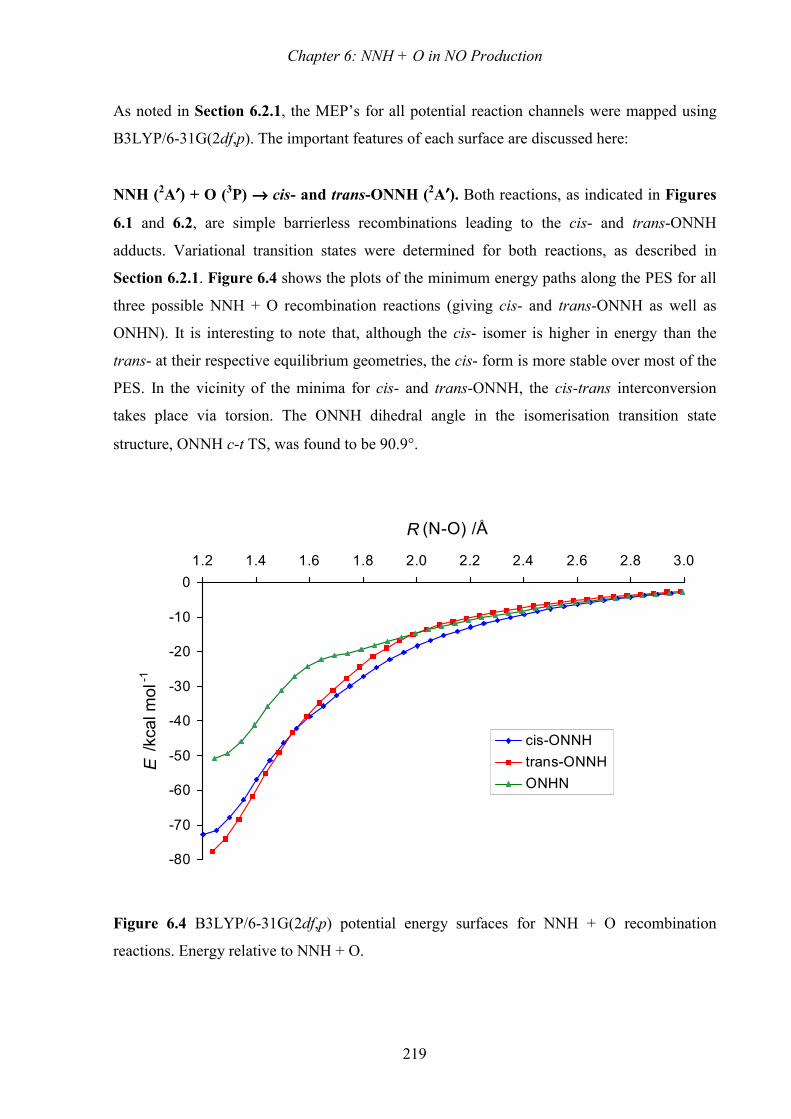
Chapter 6: NNH + O in NO Production
219
As noted in Section 6.2.1, the MEP’s for all potential reaction channels were mapped using
B3LYP/6-31G(2df,p). The important features of each surface are discussed here:
NNH (2A′′′′) + O (3P) →→→→ cis- and trans-ONNH (2A′′′′). Both reactions, as indicated in Figures
6.1 and 6.2, are simple barrierless recombinations leading to the cis- and trans-ONNH
adducts. Variational transition states were determined for both reactions, as described in
Section 6.2.1. Figure 6.4 shows the plots of the minimum energy paths along the PES for all
three possible NNH + O recombination reactions (giving cis- and trans-ONNH as well as
ONHN). It is interesting to note that, although the cis- isomer is higher in energy than the
trans- at their respective equilibrium geometries, the cis- form is more stable over most of the
PES. In the vicinity of the minima for cis- and trans-ONNH, the cis-trans interconversion
takes place via torsion. The ONNH dihedral angle in the isomerisation transition state
structure, ONNH c-t TS, was found to be 90.9°.
-80
-70
-60
-50
-40
-30
-20
-10
0
1.2 1.4 1.6 1.8 2.0 2.2 2.4 2.6 2.8 3.0
R (N-O) /Å
E /
kca
l mo
l -1
cis-ONNH
trans-ONNH
ONHN
Figure 6.4 B3LYP/6-31G(2df,p) potential energy surfaces for NNH + O recombination
reactions. Energy relative to NNH + O.

Chapter 6: NNH + O in NO Production
220
NNH (2A′′′′) + O (3P) →→→→ ONHN (2A′′′′). This is also a barrierless recombination reaction as
shown in Figures 6.3 and 6.4. The ONHN adduct and the variational transition states leading
to it are all planar 2A′ states. As shown in Figure 6.5, however, application of the time
dependent density functional approach, viz. TD-B3LYP, at the ground state geometries
reveals that the first two excited states (2A″ and 2A′ respectively) are quite close in energy to
the ground state. Figure 6.5 also suggests that there are two avoided crossings on this PES,
one at ~ 1.45 Å (between the two excited states) and one at ~ 1.65 Å (between all three
states). This indicates that, although the ground state is planar, the equilibrium geometries of
the excited state molecules are likely to be non-planar, thus raising the symmetry constraints
and allowing direct interaction between the states. In the context of the current work,
however, these unusual features are of purely academic interest, the important point being the
existence of a direct pathway leading to ONHN on the 2A′ surface.
Figure 6.5 Ground and excited state B3LYP/6-31G(2df,p) potential energy surfaces for the
NNH + O → ONHN recombination. Energy relative to NNH + O.
-60
-50
-40
-30
-20
-10
0
10
20
1.2 1.3 1.4 1.5 1.6 1.7 1.8 1.9
R(N-O) /Å
E /
kca
l mo
l -1
ground state -
first excited state -
second excited state -
2A′
2A′
2A″

Chapter 6: NNH + O in NO Production
221
cis- and trans-ONNH (2A′′′′) →→→→ NO (2ΠΠΠΠ) + NH (3ΣΣΣΣ). The dissociation of both isomers was
found to occur via a common, barrierless, non-planar surface, as shown in Figures 6.1 and
6.2. The MRCI studies of Walch12 have previously established that dissociations of both cis-
and trans-ONNH on the 2A′ surface must pass over activation barriers while the analogous
2A″ surfaces are barrierless. The same features are also observed on our B3LYP/6-31G(2df,p)
PES, shown in Figure 6.6, with the surface crossings from 2A′ to 2A″ occurring at R(N-N) ≈
1.67 Å for the trans isomer and R(N-N) ≈ 1.58 Å for cis-ONNH. When the minimum energy
path for the dissociation of the trans isomer was mapped with no symmetry constraints
applied, the trans 2A′ surface was followed until the neighbourhood of the surface crossing
from which point the molecule became non-planar and the dissociation followed a surface
very similar to that of 2A″ trans-ONNH; it therefore appears that the 2A states of the non-
planar variational transition states correlate with the 2A″ surfaces of ONNH. Such states are
accessible via torsion of the molecule, as shown in Figure 6.7. Here the potential energy
surfaces for torsion of ONNH are shown for various N-N bond lengths. At low N-N
separations there is a high barrier between 2A′ cis- and trans-ONNH; as the bond stretches,
however, the cis 2A″ surface falls below the 2A′ surface so that at R(N-N) = 1.6 Å the torsion of
2A′ trans-ONNH actually results in the cis isomer on the 2A″ surface. As the N-N bond is
stretched beyond 1.65 Å, a minimum appears on the torsional PES at a dihedral angle of
~ 130°; this is consistent with the observed non-planar variational transition states. Further
stretching of R(N-N) results in the 2A″ state of trans-ONNH falling below the 2A′ state.
Although at 1.75 Å 2A″ trans-ONNH is higher in energy than the non-planar structure, the
energy difference is only ~ 0.6 kcal mol−1; this barrier reduces further as the molecule
dissociates (as seen in Figure 6.6) such that the non-planar MEP for the dissociation is
effectively on the trans 2A″ surface. In summary, therefore, we are proposing that the
dissociation reaction of ONNH occurs via 2A′ → 2A″ surface crossing which can be achieved
by the out-of-plane distortion, viz. torsion of the molecules. This is reasonable for the sort of
systems we are modelling, where the ONNH adducts are generated in highly vibrationally
excited states as a result of chemical and/or collisional activation. Surface crossing, via
vibronic coupling, predominantly involving torsion, is expected to occur readily. Note,
however, that even though there is a common MEP for both cis and trans dissociations, their
respective variational transition states differ slightly because of the differences in the ground
state energies and partition functions of the two ONNH isomers.

Chapter 6: NNH + O in NO Production
222
-70
-60
-50
-40
-30
-20
-10
0
1.25 1.3 1.35 1.4 1.45 1.5 1.55 1.6 1.65 1.7 1.75 1.8 1.85 1.9 1.95R (N-N) /Å
E /
kca
l mo
l -1
cis - 2A'
trans - 2A'
cis - 2A"
trans - 2A"
trans - 2A' with nosymmetry constraints
cis - 2A′
trans - 2A′
cis - 2A″
trans - 2A″
trans - 2A′
Figure 6.6 B3LYP/6-31G(2df,p) 2A′ and 2A″ PES’s for ONNH → NO + NH showing the
stretching of the N-N bond in the cis- and trans-isomers and in the non-planar reaction path
for 2A′ trans-ONNH with no symmetry constraints. (Energy relative to NO + NH.)
15
20
25
30
35
40
45
50
-20 0 20 40 60 80 100 120 140 160 180 200dihedral angle /degrees
E /
kca
l mo
l -1
1.75 1.65
1.60 1.55
1.52 1.442A′
2A′
2A′
2A′
2A′
2A′
2A′
2A′
2A′
2A″
2A″
2A″
2A″
cis -ONNH trans -ONNH
Figure 6.7 B3LYP/6-31G(2df,p) torsional potentials for ONNH at various R(N-N) (in Å)
distances. (Energy relative to 2A′ trans-ONNH.)

Chapter 6: NNH + O in NO Production
223
ONHN (2A′′′′) →→→→ HNO (1A′′′′) + N (4S). This reaction (Figure 6.3) is complicated by a change
in spin multiplicity from doublet to quartet as the N-N bond breaks. By mapping the
minimum energy paths on both the doublet and quartet surfaces as a function of N-N distance,
it was found that the intersection occurs at a distance of approximately 1.94 Å (Figure 6.8).
The variational transition states for the dissociation at all temperatures are found to occur on
the (barrierless) quartet surface at N-N distances of ~ 2.1 Å. We expect that the intersystem
crossing will be substantially faster than the classical dissociation, hence the rate of this
reaction was calculated using variational transition state and RRKM theory, utilising the
transition state structures identified on the quartet surface.
-80
-70
-60
-50
-40
-30
-20
-10
0
10
1.2 1.4 1.6 1.8 2 2.2
R (NN) /Å
E /
kca
l mo
l -1
doublet surface
quartet surface
Figure 6.8 B3LYP/6-31G(2df,p) PES for ONHN → HNO + N showing the doublet and
quartet surfaces. (Energy relative to HNO + N.)
cis- and trans-ONNH (2A′′′′) →→→→ N2O (1ΣΣΣΣ) + H (2S). The dissociation of the cis isomer takes
place over a barrier of 24.4 kcal mol−1 (6.1 kcal mol−1 above products) as shown in Figure
6.2. The B3LYP calculations reveal that in this transition state, labelled ONN-H, the ONN
moiety is near-linear (A(NNO) = 173°) and the N-H separation is 1.66 Å. Attempts to find an
analogous transition state on the trans surface were, however, unsuccessful as calculations

Chapter 6: NNH + O in NO Production
224
converged either to the cis transition state or to a second order saddle point. Mapping the
minimum energy path as a function of N-H distance for trans-ONNH revealed a monotonic
increase in the energy, significantly exceeding the barrier height to ONN-H in the region of
R(N-H) ≈ 1.50 Å; at this point, however, the NNO angle of 156° is only 24° larger than at
equilibrium. Stretching the N-H bond further results in a rapid increase in the NNO angle and
collapse onto the cis surface (Figure 6.9). Further exploration of the potential energy surface
revealed that there is a family of low energy (~ 5 – 10 kcal mol−1) trans to cis isomerisation
pathways that occur via the linearisation of the NNO moiety such that the maximum energy is
below the energy of ONN-H. In summary, therefore, both cis- and trans-ONNH dissociate to
N2O + H via a common transition state as shown in Figures 6.1 and 6.2, with the
understanding that the trans to cis isomerisation is part of the overall mechanism.
-35
-30
-25
-20
-15
-10
-5
0
5
10
15
1 1.2 1.4 1.6 1.8 2
R (N-H) /Å
E /
kca
l mo
l -1
trans-ONNH
cis-ONNH
Figure 6.9 B3LYP/6-31G(2df,p) PES for ONNH → N2O + H. (Energy relative to N2O + H.)
ONHN (2A′′′′) →→→→ N2O (1ΣΣΣΣ) + H (2S). As shown in Figure 6.3, this reaction proceeds via a
transition state (denoted ON2-H) with a critical enthalpy of 21.7 kcal mol−1 and an
exothermicity of 1.4 kcal mol−1 at 298 K.

Chapter 6: NNH + O in NO Production
225
cis-ONNH (2A′′′′) →→→→ N2 (1ΣΣΣΣg) + OH (2ΠΠΠΠ). This reaction (Figure 6.1 and 6.2) occurs via a
cyclic NNOH transition state (designated NNOHsq) followed by dissociation to N2 + OH.
Given the geometry of this transition state, the reaction can only proceed from the cis form of
ONNH. The computed reaction barrier is 34.5 kcal mol−1, that is, ~ 10 kcal mol−1 higher than
for the N2O + H channel. However, while ONNH → N2O + H is endothermic, the ONNH →
N2 + OH reaction is highly exothermic (by 45.1 kcal mol−1).
ONHN (2A′′′′) →→→→ N2 (1ΣΣΣΣg) + OH (2ΠΠΠΠ). This reaction proceeds by a 1,2 hydrogen shift from the
central nitrogen to the oxygen, yielding a cyclic transition state, followed by decomposition
into N2 + OH (Figure 6.3). The transition state has been labelled NNOHtr; it is 29.4 kcal
mol−1 higher in energy than ONHN and 91.4 kcal mol−1 higher than the dissociated products.
NNH (2A′′′′) + O (3P) →→→→ N2 (1ΣΣΣΣg) + OH (2ΠΠΠΠ). This reaction represents the direct abstraction of
the hydrogen of NNH by an oxygen atom. Somewhat surprisingly, no barrier was found for
this reaction. This is likely to be a consequence of the very weak (breaking) N-H bond and the
very strong interaction between the hydrogen and oxygen atoms, which is attractive at all O-H
separations.
trans-ONNH (2A′′′′) →→→→ ONHN (2A′′′′). These two intermediates can interconvert via a 1,2
hydrogen shift, although the barrier is rather high at 53.6 kcal mol−1 above trans-ONNH and
29.3 kcal mol−1 above ONHN (Figure 6.3). We also considered the possibility that this
isomerisation could occur via a 1,2 oxygen shift. Although a transition state was found for
this process using B3LYP/6-31G(2df,p), the subsequent RCCSD(T) calculations using this
geometry showed large values of the 1τ diagnostic and are therefore judged to be unreliable.
Similarly, the corresponding higher level calculations which make up G3X were also not
accepted as reliable due to the presence of significant spin contamination. As the energy of
this transition state is ~ 28 kcal mol−1 higher than the analogous H transfer transition state at
the B3LYP level of theory, this process was not investigated any further.

Chapter 6: NNH + O in NO Production
226
6.3.3 Kinetic Parameters
For the three reaction potential energy surfaces (viz. those shown in Figures 6.1 to 6.3)
chemical activation simulations were carried out over the temperature range of 1000 – 2600 K
and at pressures ranging from 1 to 10000 Torr using the MultiWell code. This temperature
range spans the temperatures of relevance in flame studies. For each potential energy surface
there are four barrierless reactions. These are the reverse fission reactions, adduct → NNH +
O together with cis-ONNH → NO + NH, trans-ONNH → NO + NH and ONHN → HNO +
N. For each of these reactions a variational transition state (VTS) was located at temperatures
of 1000 K, 1500 K, 2000 K and at a higher temperature (2500 K except for trans-ONNH →
NO + NH and ONHN→ O + NNH which were evaluated at 2400 K and 2200 K respectively).
The VTS evaluated at 1000 K was used in the MultiWell modelling for temperatures 1000
and 1200 K, the VTS at 1500 K used for temperatures 1400 and 1600 K, the VTS at 2000 K
for temperatures 1800, 2000 and 2200 K and the high temperature VTS for 2400 and 2600 K.
Pressure-dependent overall rate coefficients to the four product channels were calculated
using Equations (6.14) and (6.15).
No stabilisation of adducts or intermediates was found at any temperature or pressure in the
studied range. Rate coefficients derived for individual reaction channels for a pressure of 1
atm are shown in Table 6.6. The rate coefficients did not show any significant pressure
dependence between 1 and 10000 Torr and were not strongly dependent on temperature. The
summed contribution to each channel from the two surfaces can be fitted by a modified
Arrhenius expression and these rate coefficients are given in Table 6.7. From Tables 6.6 and
6.7 we see that the major product channel is to N2O + H, with all three surfaces contributing
an approximately equal amount of reaction flux. The main contribution to the N2 + OH
channel is through the intermediate ONHN, with a somewhat smaller contribution arising
from the cis-ONNH. Nearly all flux to NO + NH is through the cis- and trans- adducts. The
endothermic reaction to HNO + N is only a very minor pathway and nearly all reaction flux is
via the ONHN intermediate. A significant additional contribution to the production of N2 +
OH can also arise from the barrierless direct abstraction reaction for NNH + O.

Chapter 6: N
NH
+ O
in NO
Production
227
Table 6.6 Rate coefficients (cm3 mol−1 s−1) for NNH + O → product channels shown via adducts cis-ONNH, trans-ONNH and ONHN at 1
atm pressure.
via adduct
cis-ONNH trans-ONNH
T/K NO + NH N2O + H N2 + OH HNO + N NO + NH N2O + H N2 + OH HNO + N
1000 6.51×10¹² 1.64×10¹³ 3.19×10¹² 9.45×10¹² 2.17×10¹³ 8.36×10¹¹
1200 7.23×10¹² 1.56×10¹³ 3.09×10¹² 9.35×10¹² 1.82×10¹³ 6.33×10¹¹
1400 7.07×10¹² 1.56×10¹³ 3.18×10¹² 7.65×10¹² 1.90×10¹³ 8.13×10¹¹
1600 7.88×10¹² 1.52×10¹³ 3.19×10¹² 7.60×10¹² 1.66×10¹³ 6.44×10¹¹
1800 7.62×10¹² 1.69×10¹³ 3.55×10¹² 7.55×10¹² 1.69×10¹³ 6.07×10¹¹
2000 8.16×10¹² 1.65×10¹³ 3.50×10¹² 8.09×10¹² 1.64×10¹³ 5.59×10¹¹
2200 8.84×10¹² 1.60×10¹³ 3.50×10¹² 7.45×10¹² 1.35×10¹³ 4.62×10¹¹
2400 9.40×10¹² 1.63×10¹³ 3.58×10¹² 7.15×10¹² 1.32×10¹³ 4.89×10¹¹
2600 9.77×10¹² 1.57×10¹³ 3.50×10¹² 7.05×10¹² 1.19×10¹³ 4.50×10¹¹ 2×10⁹

Chapter 6: N
NH
+ O
in NO
Production
228
Table 6.6. continued
via adduct
ONHN
T/K NO + NH N2O + H N2 + OH HNO + N
1000 3.61×10¹¹ 1.94×10¹³ 6.55×10¹²
1200 2.52×10¹¹ 1.99×10¹³ 6.13×10¹²
1400 3.00×10¹¹ 1.86×10¹³ 5.88×10¹²
1600 5.07×10¹¹ 1.70×10¹³ 5.89×10¹² −3×10⁹
1800 5.06×10¹¹ 2.10×10¹³ 7.22×10¹² −7×10⁹
2000 5.40×10¹¹ 1.83×10¹³ 6.41×10¹² −6×10⁹
2200 5.84×10¹¹ 1.60×10¹³ 6.12×10¹² 12×109
2400 5.52×10¹¹ 1.63×10¹³ 6.10×10¹² 20×109
2600 5.27×10¹¹ 1.43×10¹³ 5.48×10¹² 16×109

Chapter 6: NNH + O in NO Production
229
Table 6.7 Modified Arrhenius parameters for NNH + O → products via adducts cis-ONNH,
trans-ONNH and ONHN ( ( )expnak AT E RT= − ).
Reactions A/cm3 mol−1 s−1 n Ea/cal mol−1
NNH + O → NO + NH 7.80×10¹⁰ 0.642 −1830.
NNH + O → N2O + H 2.40×10¹⁶ −0.765 1540.
NNH + O → N2 + OH 2.57×10¹⁰ 0.702 −2320.
NNH + O → HNO + N 6.2×10⁻⁷ 4.84 0.
NNH + O → N2 + OH a 3.00×10¹³ 0 0.
a Direct abstraction reaction via abstraction transition state.
Our branching ratios into the three principal reaction channels are very different from those
estimated by Bozzelli and Dean.2 In their QRRK analysis they only considered a single
ONNH adduct. They also did not consider the ONHN adduct which we have discovered in the
present work. The ONHN well is considerably shallower than that for cis- or trans-ONNH
and significant flux flows through the ONHN adduct both to N2O + H and to N2 + OH (but
not to NO + NH).
6.3.4 Comparison with Experiment
As mentioned in the Introduction (Section 6.1), Hayhurst and Hutchinson5 reported a value
for 4 ,3Pk K from which they then estimated a rate coefficient, 4k , for reaction to NO + NH.
Their method involved the assumption that every NH radical produced by Reaction (6.4)
rapidly reacts to yield a second NO molecule. For fuel-rich flames of CH4 / O2 / N2 and of H2
/ O2 / N2 the above assumption leads to the equation
4 ,3 42 H
[NO] 1 1
2[N ][O]P
dk K k
dt x
= ⋅ − ⋅
(6.17)
where Hx is the mole fraction of H in the burnt gas. To obtain Hx , Hayhurst and Hutchinson
measured OH and temperature profiles in the burnt gas. There are, however, very significant

Chapter 6: NNH + O in NO Production
230
random errors in their data, ranging from nearly 3 orders of magnitude at 2500 K to nearly an
order of magnitude at 1800 K. If we fit our computed values of 4k from the MultiWell
simulations and ,3PK derived from our thermochemical calculations we obtain
( )74 ,3 3.7 10 exp 2800Pk K T= × − cm3 mol−1 s−1. Comparing with Hayhurst and Hutchinson’s
value of ( )94 ,3 1.4 10 exp 2760Pk K T= × − cm3 mol−1 s−1 shows that our value at 2000 K is
over an order of magnitude lower than theirs but probably still within the considerable
random error in their data.
6.3.5 Kinetic Modelling
As discussed earlier, detailed chemical reaction models, such as the two formulations of
GRIMech3,4 (containing the rate coefficient for 4k estimated by Bozzelli and Dean2), have
recently been found to overestimate the level of NO produced by combustion systems. We
have chosen to use the GRIMech 3.0 model with our new NNH thermochemistry and kinetics.
The value of 4k in this model was altered to the value given in Table 6.7 and the other three
addition and decomposition reaction channels also included together with the direct
abstraction of H by O atoms. This modified mechanism has been used to model two series of
data54 from a completely stirred reactor – a fuel lean methane / air combustion and a lean
combustion of CO / H2 / air at residence times, τ, between about 3 to 4 ms and equivalence
ratios, φ, between 0.5 and 0.6 approximately. The first of these cases has been used to
benchmark the performance of GRIMech.4 Figure 6.10 compares the performance of our
modified kinetic model with that of the original GRIMech 3.0 formulation and experimental
NO profiles.
As can be seen from Figure 6.10(a) both the original formulation of GRIMech 3.0 and our
modified version with new NNH thermochemistry and kinetics reproduce the experimental
NO data from CH4 / air satisfactorily although our model gives a closer fit to experiment.
With the runs in CO / H2 / air (Figure 6.10(b)), however, significantly poorer performance
occurs when using the original GRIMech 3.0 model. Whereas our present model gives a good
fit to experiment, GRIMech 3.0 overestimates the level of NO by nearly a factor of two. To

Chapter 6: NNH + O in NO Production
231
ascertain the reason for this difference in performance we have carried out reaction path
analyses on both kinetic models.
1650 1700 1750 18000
5
10
15
NO
/pp
m
(a)CH4/air
0.512 ≤φ≤ 0.6223.22 ≤τ≤ 3.54 ms
1660 1680 1700 1720T/K
0
10
20
30
40
50
60
70
NO
/pp
m
(b)air/CO = 82/17.4 mol %H2 = 0.69 - 0.25 mol %
3.87 ≤τ≤ 4.03 ms
Figure 6.10 Comparison of NO profiles of combustion in a completely stirred flame reactor.
(a) CH4 / air, (b) H2 / CO / air. Filled circles: Experimental data from Ref. 54. Dashed lines:
predictions using GRIMech 3.0. Full lines: prediction using GRIMech 3.0 with NNH
thermochemistry and kinetics from the present study.

Chapter 6: NNH + O in NO Production
232
We have sought to quantify the contribution that each of the four reaction pathways
(Zel’dovich, Prompt-NO, N2O and NNH + O) makes to NO production by using the
following simplified procedure. In order to determine the contribution of a particular pathway,
that pathway is eliminated from the kinetic model and the modified mechanism is then run to
ascertain the effect of its omission. This is repeated in turn for each pathway. The basic
assumption in this method is that there are no cross correlations between the pathways. It has
been shown, however, that the error resulting form such neglect of cross correlation is of 5%
or less in the total contribution of all pathways when applied to NO profiles in atmospheric
opposed flow methane-air flames.55 In our present path analysis the summation error is
significantly less than 3%.
The contribution of the thermal pathway is assessed by eliminating its initiation reaction,
(6.1). The prompt-NO pathway contribution was also determined by elimination of its
initiation reaction, (6.2). To assess the contribution of the N2O intermediate pathway, it was
necessary to eliminate all reactions involving N2O from the reaction model while the NNH +
O route was quantified by elimination of its initiation reaction, (6.4). This procedure is
similar to that used previously.6, 55
Figures 6.11(a) and (b) compare the contribution of each reaction pathway for our present
model and for the original formulation of GRIMech 3.0 to methane-air studies in a completely
stirred reactor.54 The computed contributions of the N2O intermediate, thermal and prompt-
NO pathways are similar for both models. A larger contribution of the NNH + O pathway is
calculated using GRIMech 3.0. Nevertheless, because the first three pathways all make
significant contributions to the NO profile, the two models both give reasonable reproductions
of the experimental data, although GRIMech 3.0 does somewhat overestimate the NO levels.
It is with the runs in CO / H2 / air (Figure 6.11(c) and (d)), however, that the computed
contributions of the two models radically differ. The prompt-NO pathway makes no
contribution in these runs. Again, the calculated contributions of the N2O and thermal
pathways are quite similar for both models, however GRIMech 3.0 predicts that the NNH + O
pathway will make the greatest contribution to the NO profiles whereas our model, with new
NNH thermochemistry and kinetics, predicts that this pathway makes only a very small
contribution to the total. It is apparent, therefore, that by overestimating the contribution of
the NNH + O pathway GRIMech 3.0 predicts too high a level of NO in this system. In
methane-air combustion, where there are significant contributions from the prompt and

Chapter 6: NNH + O in NO Production
233
thermal routes, the overestimation of the NNH + O pathway is masked. Where the prompt and
thermal pathways are minimised this overestimation becomes obvious. A detailed testing of
our new thermochemistry and kinetics in modelling premixed and opposed flow flames will
be presented elsewhere.56
1650 1700 1750 18000
5
10
15
NO
/pp
m
TotalNNH + ON2O intermediatePrompt-NOThermal
(a)
1650 1700 1750 18000
5
10
15 (b)
1660 1680 1700 1720
T/K
0
10
20
30
40
50
60
70(c)
Prompt-NO
1660 1680 1700 17200
10
20
30
40
50
60
70(d)
Prompt-NO
Figure 6.11 Predictions of the contribution of individual pathways to NO formation.
(a) Present model predictions for the CH4 / air data of Figure 6.10(a).
(b) GRIMECH 3.0 predictions for the CH4 / air data of Figure 6.10(a).
(c) Present model predictions for the H2 / CO / air data of Figure 6.10(b).
(d) GRIMECH 3.0 predictions for the H2 / CO / air data of Figure 6.10(b).

Chapter 6: NNH + O in NO Production
234
6.4 Conclusions
Three reaction potential energy surfaces for NNH + O → products have been investigated by
ab initio quantum chemical calculations. Three adducts, namely trans-ONNH, cis-ONNH and
ONHN, have been identified through which reaction to three exothermic product channels,
NO + NH, N2 + OH, N2O + H, and one endothermic channel, HNO + N, takes place. Rate
coefficients to each reaction channel have been obtained by RRKM analysis. The rate
coefficient at 2000 K to the NO + NH channel is predicted to be approximately a factor of
four lower than had been previously estimated2 (and included in detailed reaction models such
as GRIMech 3.0)4. A new value of 0298f H∆ (NNH) = 60.6 ± 0.5 kcal mol−1 has been obtained
by CCSD(T) calculations which include extrapolation to the complete basis limit. This value,
together with the rate coefficients we have derived for the NNH + O → products reactions,
have been used to modify the GRIMech 3.0 reaction model. Using this new formulation we
could satisfactorily model NO profiles produced in a completely stirred reactor54 from both
methane / air and CO / H2 / air mixtures. Overestimation of NO profiles from the latter
mixtures by GRIMech 3.0 has been shown, by reaction path analysis, to result from too high a
rate coefficient for initiation of the NNH + O pathway. On the basis of the present work we
conclude that this pathway represents a very minor route to NO in most combustion systems.

Chapter 6: NNH + O in NO Production
235
6.5 References
1. J. A. Miller and C. T. Bowman, Prog. Energy Combust. Sci., 1989, 15, 287.
2. J. W. Bozzelli and A. M. Dean, Int. J. Chem. Kinet., 1995, 27, 1097.
3. C. T. Bowman, R. K. Hanson, D. F. Davidson, W. P. Gardiner, Jr, V. Lissianski, G. P.
Smith, D. M. Golden, M. Frenklach and M. Goldenberg, GRIMech 2.11,
http://www.me.berkeley.edu/gri_mech.
4. G. P. Smith, D. M. Golden, M. Frenklach, N. W. Moriaty, B. Eiteneer, M.
Goldenberg, C. T. Bowman, R. K. Hanson, S. Song, W. C. J. Gardiner, V. V.
Lissianski and Z. Qin, GRIMech 3.0, http://www.me.berkeley.edu/gri_mech/.
5. A. N. Hayhurst and E. M. Hutchinson, Combust. Flame, 1998, 114, 274.
6. D. Charlston-Goch, B. L. Chadwick, R. J. S. Morrison, A. Campisi, D. D. Thomsen
and N. M. Laurendeau, Combust. Flame, 2001, 125, 729.
7. A. A. Konnov and J. De Ruyck, Combust. Flame, 2001, 125, 1258.
8. C. F. Melius and J. S. Binkley, in Twentieth Symp. (Int.) on Combustion; The
Combustion Institute: Pittsburgh, Pennysylvania, 1984, p. 575.
9. P. Marshall, A. Fontijn and C. F. Melius, J. Chem. Phys., 1987, 86, 5540.
10. T. Fueno, M. Fukuda and K. Yokoyama, Chem. Phys., 1988, 124, 265.
11. J. A. Harrison and R. G. A. R. MacIagan, J. Chem. Soc. Faraday Trans., 1990, 86,
3519.
12. S. P. Walch, J. Chem. Phys., 1993, 98, 1170.
13. J. L. Durant, Jr., J. Phys. Chem., 1994, 98, 518.
14. K. S. Bradley, P. McCabe, G. C. Schatz and S. P. Walch, J. Chem. Phys., 1995, 102,
6696.
15. M. Simonson, K. S. Bradley and G. C. Schatz, Chem. Phys. Lett., 1995, 244, 19.
16. S. Kristyan and M. C. Lin, Chem. Phys. Lett., 1998, 297, 200.
17. M. C. van Beek and J. J. ter Meulen, J. Chem. Phys., 2001, 115, 1843.
18. S. P. Walch and H. Partridge, Chem. Phys. Lett., 1995, 233, 331.
19. J. Gu, Y. Xie and H. F. Schaefer, III, J. Chem. Phys., 1998, 108, 8029.
20. L. A. Curtiss, P. C. Redfern, K. Raghavachari and J. A. Pople, J. Chem. Phys., 2001,
114, 108.
21. C. Hampel, K. A. Peterson and H.-J. Werner, Chem. Phys. Lett., 1992, 190, 1.

Chapter 6: NNH + O in NO Production
236
22. K. Raghavachari, G. W. Trucks, J. A. Pople and M. Head-Gordon, Chem. Phys. Lett.,
1989, 157, 479.
23. T. H. Dunning, Jr., J. Chem. Phys., 1989, 90, 1007.
24. R. A. Kendall, T. H. Dunning, Jr. and R. J. Harrison, J. Chem. Phys., 1992, 96, 6796.
25. D. E. Woon and T. H. Dunning, Jr., J. Chem. Phys., 1993, 98, 1358.
26. A. D. Becke, J. Chem. Phys., 1993, 98, 5648.
27. A. D. Becke, Phys. Rev. A, 1988, 38, 3098.
28. C. Lee, W. Yang and R. G. Parr, Phys. Rev. B, 1988, 37, 785.
29. T. Helgaker, W. Klopper, H. Koch and J. Noga, J. Chem. Phys., 1997, 106, 9639.
30. R. D. Cowan and D. C. Griffin, J. Opt. Soc. Am., 1976, 66, 1010.
31. R. L. Martin, J. Phys. Chem., 1983, 87, 750.
32. B. O. Roos, P. R. Taylor and P. E. M. Siegbahn, Chem. Phys., 1980, 48, 157.
33. B. O. Roos, in Ab initio Methods in Quantum Chemistry II, K. P. Lawley, Ed.;
Advances in Chemical Physics, I. Prigogine and S. A. Rice, Eds.; Vol. LXIX; J. Wiley
& Sons Ltd.: Chichester, UK, 1987, p. 399.
34. L. A. Curtiss, K. Raghavachari, P. C. Redfern, V. Rassolov and J. A. Pople, J. Chem.
Phys., 1998, 109, 7764.
35. E. Pollack, in Theory of Chemical Reaction Dynamics, M. Baer, Ed.; Vol. 3; CRC
Press, Inc.: Boca Raton, Florida, 1985, p. 128.
36. W. L. Hase, S. L. Mondro, R. J. Duchovic and D. M. Hirst, J. Am. Chem. Soc., 1987,
109, 2916.
37. D. G. Truhlar and B. C. Garrett, Acc. Chem. Res., 1980, 13, 440.
38. J. C. Mackie, G. B. Bacskay and N. L. Haworth, J. Phys. Chem. A, 2002, 106, 10825.
39. J. I. Steinfeld, J. S. Francisco and W. L. Hase, Chemical Kinetics and Dynamics;
Prentice Hall: Engelwood Cliffs, NJ, 1989, 308.
40. M. J. Frisch, G. W. Trucks, H. B. Schlegel, G. E. Scuseria, M. A. Robb, J. R.
Cheeseman, V. G. Zakrzewski, J. A. Montgomery, R. E. Stratmann, J. C. Burant, S.
Dapprich, J. M. Millam, A. D. Daniels, K. N. Kudin, M. C. Strain, O. Farkas, J.
Tomasi, V. Barone, M. Cossi, R. Cammi, B. Mennucci, C. Pomelli, C. Adamo, S.
Clifford, J. Ochterski, G. A. Petersson, P. Y. Ayala, Q. Cui, K. Morokuma, D. K.
Malick, A. D. Rabuck, K. Raghavachari, J. B. Foresman, J. Cioslowski, J. V. Ortiz, B.
B. Stefanov, G. Lui, A. Liashenko, P. Piskorz, I. Komaromi, R. Gomperts, R. L.
Martin, D. J. Fox, T. Keith, M. A. Al-Laham, C. Y. Peng, A. Nanayakkara, C.
Gonzalez, M. Challacombe, P. M. W. Gill, B. G. Johnson, W. Chen, M. W. Wong, J.

Chapter 6: NNH + O in NO Production
237
L. Andres, M. Head-Gordon, E. S. Replogle and J. A. Pople, Gaussian 98 Revision
A.7, Gaussian, Inc.: Pittsburgh, PA, 1998,
41. P. J. Knowles, C. Hampel and H.-J. Werner, J. Chem. Phys., 1993, 99, 5219.
42. MOLPRO 96.3 is a package of ab initio programs written by H.-J. Werner and P. J.
Knowles with contributions from J. Almlöf, R. D. Amos, M. J. O. Degan, S. T. Elbert,
C. Hampel, W. Meyer, K. Peterson, R. Pitzer, A. J. Stone, P. R. Taylor, R. Lindh, M.
E. Mura, T. Thorsteinsson.
43. "DALTON, an ab initio electronic structure program, Release 1.0 (1997)" written by
T. Helgaker, H. J. Aa. Jensen, P. Joergensen, J. Olsen, K. Ruud, H. Aagren, T.
Andersen, K. L. Bak, V. Bakken, O. Christiansen, P. Dahle, E. K. Dalskov, T.
Enevoldsen, B. Fernandez, H. Heiberg, H. Hettema, D. Jonsson, S. Kirpekar, R.
Kobayashi, H. Koch, K. V. Mikkelsen, P. Norman, M. J. Packer, T. Saue, P. R. Taylor
and O. Vahtras.
44. K. Andersson, M. R. A. Blomberg, M. P. Fülscher, G. Karlström, R. Lindh, P.-Å.
Malmqvist, P. Neogrády, J. Olsen, B. O. Roos, A. J. Sadlej, M. Schültz, L. Seijo, L.
Serrano-Andrés, P. E. M. Siegbahn and P.-O. Widmark, MOLCAS Version 4, Lund
University: Lund, Sweden, 1997,
45. J. R. Barker, Multiwell Software Version 1.2.0, Ann Arbor, MI, 2002,
http://aoss.engin.mumich.edu/multiwell/.
46. J. R. Barker, Int. J. Chem. Kin., 2001, 33, 232.
47. R. J. Kee, F. M. Rupley, J. A. Miller, M. E. Coltrin, J. F. Grcar, E. Meeks, H. K.
Moffat, A. E. Lutz., G. Dixon-Lewis, M. D. Smooke, J. Warnatz, G. H. Evans, R. S.
Larson, R. E. Mitchell, L. R. Petzold, W. C. Reynolds, M. Caracotsios, W. E. Stewart,
P. Glarborg, C. Wang and O. Adigun, CHEMKIN Collection Release 3.6, Reaction
Design, Inc.: San Diego, CA, 2000,
48. R. Tarroni, P. Palmieri, A. Mitrushenkov, P. Tosi and D. Barsi, J. Chem. Phys., 1997,
106, 10265.
49. M. W. Chase, Jr., J. Phys. Chem. Ref. Data, 1998, Monograph 9, 1.
50. B. Rusic, D. Feller, D. A. Dixon, K. A. Peterson, L. B. Harding, R. L. Asher and A. F.
Wagner, J. Phys. Chem. A, 2001, 105, 1.
51. W. R. Anderson, Combustion and Flame, 1999, 117, 394.
52. A. K. Wilson, T. van Mourik and T. H. Dunning, Jr., J. Molec. Struct. (Theochem),
1996, 388, 339.
53. T. van Mourik, A. K. Wilson and T. H. Dunning, Jr., Mol. Phys., 1999, 96, 529.

Chapter 6: NNH + O in NO Production
238
54. R. C. Steele, P. C. Malte, D. G. Nicol and J. C. Kramlich, Combust. Flame, 1995, 100,
440.
55. D. D. Thomsen and N. M. Laurendeau, Combust. Flame, 2001, 124, 350.
56. J. C. Mackie, N. L. Haworth and G. B. Bacskay, 2003 Australian Symposium on
Combustion & The 8th Australian Flames Days, Melbourne, December 8-9, 2003.
7 The Enthalpy and Mechanism of the
Photolysis of CFClBr2
Chapter 7
The Enthalpy and
Mechanism of the
Photolysis of CFClBr2

Chapter 7. Photolysis of CFClBr2
240
The work described in this chapter represents a combined experimental and theoretical
investigation into the thermochemistry of the bromomethane CFClBr2. It is being jointly
published in Chemical Physics Letters.1 The experimental work (Section 7.2) was performed
by N. L. Owens, K. Nauta and S. H. Kable and has also been reported in the Honours thesis of
Owens2. The theoretical and experimental aspects of this work are heavily interreliant and
thus the work has been reported here in its entirety.
7.1 Introduction
The role of halons and CFC’s in the chemistry of the atmosphere has been well documented
for many decades. As a general class of molecules, halomethanes absorb ultraviolet light via a
σ*←σ transition, which results in the cleavage of the weakest C−X bond (where X is halogen
or hydrogen). The fate of the atom is very well understood and central to the depletion of
stratospheric ozone. The fate of the halomethyl radical is less well understood, but the
primary reaction is probably O2 addition leading to the formation of halogen-substituted
aldehydes and slow transport back to the troposphere.
Over the past couple of decades, several reports of UV or vacuum-UV excitation of
halomethanes, resulting in cleavage of two C–X bonds, have appeared. Bromo- and
iodomethane species seem to exhibit triple fragmentation pathways when the wavelength is
shorter than 200 nm.3-10 For wavelengths longer than 200 nm, however, only the difluoro-
species, CF2I2, CF2Br2 and CF2BrI have been reported to undergo triple fragmentation. CF2I2
undergoes a single C–I cleavage at longer wavelengths, which is believed to become two
sequential C–I cleavages and finally concerted loss of two I-atoms as the energy of the
dissociating photon is increased.10 Triple fragmentation of CF2Br2 and CF2BrI are also
thought to be stepwise processes.5-9

Chapter 7. Photolysis of CFClBr2
241
In a series of papers on carbene spectroscopy, Kable and co-workers have created carbenes by
photolysis of suitable halon precursors, for example CFCl from CFClBr2,11 and both CHF and
CFBr from CHFBr2.12 At the time, no attempt was made to elucidate the mechanism of
carbene formation. In this paper we investigate the mechanism by which CFCl is formed from
CFClBr2 (halon-1112).
Interpretation of the results is made more difficult by the absence of thermochemical data
concerning halon-1112. In fact, we could locate thermochemical data for only two
dibromomethane compounds: CF2Br2 13 and CH2Br2
14. The literature thermodynamic data
for carbenes, including CFCl, are also highly varying. The most reliable current values are
probably theoretical values obtained by Dixon et al. for CF2,15,16 CHBr and CBr2
17 and by
Sendt and Bacskay18 for CFCl. Both groups utilised the coupled cluster method with
extrapolation to the complete basis limit and expect their results to be accurate to within ± 4
kJ mol−1. The Gaussian-3 (G3) calculations of Sendt and Bacskay18 for CF2 and CFCl and the
Gaussian-2 results of Cameron and Bacskay19 for CHBr and CBr2 are in good agreement with
these coupled cluster results. More recently, the G3 procedure has been extended to be able to
describe molecules containing atoms from the third row.20 We have therefore calculated bond
energies and heats of formation for a number of molecules containing bromine atoms using
the G3 methodology. In addition to facilitating the interpretation of the experimental data, the
calculations also permit us to test the accuracy of the G3 method for larger bromine
containing molecules, especially since the largest in the G3 test set is CH3Br.
The objectives of the current work are threefold. Firstly we seek to establish whether there is a
triple fragmentation pathway for CFClBr2 following absorption of a single photon at
stratospherically relevant wavelengths. Secondly, we use these data to determine
thermochemical properties for the various species involved, including heats of formation and
bond energies. Finally, we calculate those same thermochemical properties using the new
formulation of G3 theory for third row atoms to verify both the experimental data and the
validity of the theoretical method for larger bromine-containing compounds.

Chapter 7. Photolysis of CFClBr2
242
7.2 Experimental Methods and Results
7.2.1 Methodology
Details of the experiment can be found in the previous work on CFCl of Guss et al.11 Very
briefly, helium (2 bar) was bubbled through CFClBr2 (l, 0°C) and expanded via a pulsed
nozzle into a vacuum chamber. CFClBr2 was photolysed at the nozzle orifice by a Nd:YAG
pumped OPO laser (Coherent Infinity 40-100 and OPASCAN). The output of the OPO was
varied from 480 to 560 nm and frequency doubled to yield light from 240 to 280 nm. The
ensuing CFCl fragments were probed about 10 mm downstream, approx. 6 µs after the
photolysis pulse, by an excimer pumped dye laser (Lambda Physik Lextra 200 and LPD
3001E, Exalite 398 dye). By allowing the CFCl to cool in the expansion, any effect of
different CFCl product state distributions as a function of photolysis energy is negated. The
trade-off in doing this is that the parent CFClBr2 is fairly warm (we estimate 100-200 K).
Fluorescence from CFCl was imaged onto the slits of a Spex Minimate monochromator with
5 mm slits, which acts like a 20 nm triangular bandpass filter. This filter provides no real
rotational or vibrational resolution for the CFCl fluorescence. The broadband fluorescence
was detected by an EMI 9789QB photomultiplier, the signal passed to an SRS-250 boxcar
averager and finally to an SRS-245 A/D board and a personal computer. The experiment was
timed using the internal variable delays provided by the Infinity laser.
7.2.2 Results
An absorption spectrum of CFClBr2, diluted in air, measured on a Cary 4E spectrometer, is
shown in Figure 7.1 (top). The spectrum shows negligible absorption in the actinic range (λ >
295 nm) and no sharp features, which is typical of halon and CFC species. At least two broad
overlapping features are evident, the one to the red (around 240 nm) forming a pronounced
shoulder on the stronger feature to the blue, which peaks further to the blue than the range of
the spectrometer. By analogy with other CFC’s and halons, these features are likely to be
σ*←σ transitions involving a C–Br bond.

Chapter 7. Photolysis of CFClBr2
243
240 250 260 270 2800.0
0.2
0.4
0.6
0.8
1.0
LIF
/ A
bsor
ptio
n
Wavelength (nm)
0.0
0.2
0.4
0.6
0.8
1.0 LIF signal Absorption
LIF
Sig
nal (
arb.
)
210 240 270 3000.0
0.5
1.0
1.5
2.0
2.5
Abs
orpt
ion
(arb
.)
Figure 7.1 (top) CFClBr2 absorption spectrum; (centre) fluorescence excitation spectrum of
CFClBr2; (bottom) ratio of fluorescence signal to absorption signal.

Chapter 7. Photolysis of CFClBr2
244
The photolysis of CFClBr2 is known to result in the formation of CFCl.11 Several LIF spectra
of CFCl produced in this way are shown in Figure 7.2. The origin region is shown, which is
quite weak due to poor Franck-Condon overlap with the ground state. However, it is relatively
uncongested, least affected by chlorine isotopic features, and also has well-assigned hot bands
and so we have concentrated on this region. The spectral features pertinent to this work are
the origin transition and a variety of hot-band transitions emanating from the υ2 = 1 and υ3 = 1
levels (ν2 = bend, ν3 = C–Cl stretch). The main rotational sub-branches are indicated by a
comb. The main feature is the strong rQ0 sub-branch, flanked by the rQ1 to shorter wavelength
and the pQ1 to longer wavelength. The reader is referred to previous work on CFCl
spectroscopy11 for any further details.
The mechanism of CFCl production from CFClBr2 was not explored previously. The first test
that was performed was to establish the dependence of the CFCl signal on pump laser power.
The LIF signal from the central peak of the 000 transition was monitored as the pump power
was varied randomly. The resulting dependence is shown in Figure 7.3 and indicates that the
observed signal varies linearly with laser power.
The LIF intensity from 000 transition was also monitored as the pump wavelength was
changed randomly between 240 and 275 nm as shown in Figure 7.1 (centre). The data points
in the figure arise from about 1000 laser shots and were take taken every 2 nm below 260 nm
and then every 1 nm above 260 nm. For comparison, the absorption spectrum is also plotted
on the same axes, arbitrarily normalised to the value at 240 nm. The shapes of the two spectra
are similar, but the excitation spectrum rises more rapidly towards 240 nm than does the
absorption spectrum. Additionally, the excitation spectrum has reached zero (no CFCl
observed) at 275 nm while the absorption spectrum is still about 10% of the 240 nm value
and, as shown in the top panel, continues well beyond 280 nm. The actual wavelength at
which the excitation spectrum reaches zero is rather difficult to determine in this spectrum as
the data converge asymptotically to zero over about 5 nm.
The difference between the excitation and absorption spectrum is accentuated in Figure 7.1
(bottom) by plotting the ratio of the excitation to absorption intensity. Quite clearly, relative
to the absorption spectrum, the intensity of the excitation spectrum drops consistently from
240 to 260 nm and then drops quite sharply towards 275 nm. The line is a heavily smoothed

Chapter 7. Photolysis of CFClBr2
245
395 396 397
22
03
0
1
31
1
00
0
21
1
x15
x4
240 nm
260 nm
270 nm
Wavelength (nm)
Figure 7.2 CFCl fluorescence excitation spectra in the origin region following dissociation in
CFClBr2 at 240, 260 and 270 nm.
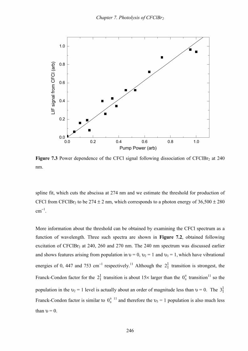
Chapter 7. Photolysis of CFClBr2
246
0.0 0.2 0.4 0.6 0.8 1.00.0
0.2
0.4
0.6
0.8
1.0
LIF
sig
nal f
rom
CF
Cl (
arb
)
Pump Power (arb)
Figure 7.3 Power dependence of the CFCl signal following dissociation of CFClBr2 at 240
nm.
spline fit, which cuts the abscissa at 274 nm and we estimate the threshold for production of
CFCl from CFClBr2 to be 274 ± 2 nm, which corresponds to a photon energy of 36,500 ± 280
cm−1.
More information about the threshold can be obtained by examining the CFCl spectrum as a
function of wavelength. Three such spectra are shown in Figure 7.2, obtained following
excitation of CFClBr2 at 240, 260 and 270 nm. The 240 nm spectrum was discussed earlier
and shows features arising from population in υ = 0, υ2 = 1 and υ3 = 1, which have vibrational
energies of 0, 447 and 753 cm−1 respectively.11 Although the 112 transition is strongest, the
Franck-Condon factor for the 112 transition is about 15× larger than the 0
00 transition11 so the
population in the υ2 = 1 level is actually about an order of magnitude less than υ = 0. The 113
Franck-Condon factor is similar to 000 11 and therefore the υ3 = 1 population is also much less
than υ = 0.

Chapter 7. Photolysis of CFClBr2
247
At 260 nm the relative population in these vibrational levels has not changed much, although
the overall signal is reduced by a factor of about four. The 270 nm spectrum, however, shows
CFCl population only in the υ = 0 and υ2 = 1 levels, with the 000 transition dominant. The
overall signal is now about 15 times reduced in comparison with the 240 nm spectrum.
The data above are summarised in Figure 7.4. A photon energy of 36,360 cm−1 (275 nm) does
not lead to detectable CFCl. At 37,037 cm−1 (270 nm) CFCl in the υ = 0 and υ2 = 1 states are
produced and at 38,460 cm−1 (260 nm), υ = 0, υ2 = 1 and υ3 = 1 levels are populated. The
energy level diagram shows that all three observations are satisfied if the combined
dissociation energy for both C–Br bonds is 36,475 ± 120 cm−1. This is in good agreement with
the threshold from the excitation spectrum of Figure 7.1, which was 36,500 ± 280 cm−1.
Figure 7.4 Energy level diagram of CFClBr2 and various reaction products calculated in this
work.

Chapter 7. Photolysis of CFClBr2
248
There are two concerns at this stage about proclaiming this to be an unambiguous
experimental measurement of the threshold to triple fragmentation of CFClBr2: i) the
observation of a linear power dependence for CFCl production is a necessary but not
sufficient condition for the process to be single photon, and ii) we have not addressed the
possibility that CFCl is produced in concert with the Br2 molecule, rather than two Br atoms.
These issues could be resolved by detailed consideration of the thermochemistry of the
appropriate processes. In the absence of reliable heats of formation for CFClBr2 or CFClBr
we have carried out high level ab initio calculations of these properties, which are presented
in the next section. The theoretical and experimental data are tied together to resolve these
issues in the Discussion.
7.3 Theoretical Methods and Results
7.3.1 Methodology
The G3 procedure for molecules with third row atoms has only been developed very
recently.20 The method is essentially the same as that initially proposed for first and second
row atoms21, where the energy of a hypothetical QCISD(T) calculation with a large basis set
is approximated by performing such a calculation with a significantly smaller basis set,
followed by corrections for enlargement of the basis set, which are computed at lower levels
of theory, namely MP2 and MP4. The G3 energy can be summarised as
[ ] [ ][ ] [ ]{ }[ ] [ ]{ }[ ] [ ]
[ ] [ ]
0 G3 QCISD(T)/6-31G( )
MP4/6-31 G( ) MP4/6-31G( ) ( correction)
MP4/6-31G(2 , ) MP4/6-31G( ) (2 , correction)
MP2(Full)/GTLarge MP2/6-31G(2 , )(G3L
MP2 6-31 G MP2 6-31G
E E d
E d E d
E df p E d df p
E E df p
E d E d
=
+ + − +
+ −
− + − / + ( ) + / ( )
ZPE SO hlc
arge correction)
E E E+ ∆ + ∆ + ∆
(7.1)

Chapter 7. Photolysis of CFClBr2
249
where the appropriate corrections due to successive basis set enlargement are evaluated at the
MP4 and MP2 levels of theory. ZPEE∆ is the zero point vibrational energy, SOE∆ denotes
spin-orbit coupling corrections and hlcE∆ is an (empirical) higher level correction.
The geometry and zero point vibrational energy are determined at the MP2(Full)/6-31G(d)
and HF/6-31G(d) levels of theory respectively. Note that the G3 formulation for third row
atoms recommends the use of a new set of basis functions20 which are based on the 6-31G
basis of Rassolov et al.22 As for first and second row atoms, the G3 calculations on molecules
containing third row atoms are performed with six d and seven f functions, except in the case
of G3Large calculations which utilise the spherical harmonic representation for all orbitals,
viz. (5d, 7f). Furthermore, following the work of Duke and Radom23, who noted an
improvement in the accuracy of the G2 procedure when the 3d electrons of third row atoms
were unfrozen to correlation, the G3 procedure also prescribes the inclusion of the 3d orbitals
of third row atoms in the valence space.
Once G3 absolute energies have been calculated, atomisation energies and thus heats of
formation can be evaluated using the relevant (experimental) atomic data. Heats of formation
can also be determined on the basis of reaction enthalpies, preferably those of isodesmic
reactions where the number of bonds of each type are conserved in the reaction. Errors in the
theoretical description of a particular atom or bond are then expected to cancel, resulting
potentially in a relatively accurate estimate of the heat of the reaction. Application of Hess’
Law then allows the determination of the heat of formation of a given species, provided
accurate (experimental) heats of formation are available for all other species in the reaction.
Isodesmic reaction schemes have been used in this work to confirm the reliability of the heats
of formation obtained from G3 atomisation energies.
The quantum chemical computations were carried out using the Gaussian98 suite of
programs24 on DEC alpha 600/5/333 and COMPAQ XP100/500 workstations of the
Theoretical Chemistry group at the University of Sydney and on the COMPAQ AlphaServer
SC system of the Australian Partnership for Advanced Computing National Facility at the
National Supercomputing Centre, ANU, Canberra

Chapter 7. Photolysis of CFClBr2
250
7.3.2 Results
The computed G3 total energies, atomisation energies and heats of formation at 0 and 298K
are reported in Table 7.1. The absolute energies of Br2, Br and CH3Br have been reported
earlier by Curtiss et al.20 As they did not report the atomisation energies or heats of formation
of Br and CH3Br, we have generated these additional data and include them here for
completeness. The G3 results for CFCl, CH4, CH2F2, CH3Cl, CH2Cl2 and CF4 have also been
published previously18,21 but are quoted here because of their importance in the decomposition
reactions of CFClBr2 and in the isodesmic reaction schemes.
Table 7.1 Energies, atomisation energies and heats of formation (at 0 and 298K) (kJ mol−1
unless otherwise noted).
−
Species 0E /Eh AE00f H∆ a 0
298f H∆
G3 G3 G3 G3/AE a G3/ID b Experimental
CFClBr2 −5745.04026 1319.2 −187.4 −188.2 −190.6 −184 ± 5
CFClBr −3171.42502 1062.5 −42.5 −−42.9
CFCl −−597.83777 −879.2 28.9 −−29.8 31 ± 13c
Br2 −5147.10746 −190.4 33.3 −−34.6 30.91 ± 0.11d
Br −2573.51747 111.8 111.87 ± 0.12d
CH3Br −2613.41950 1500.0 −28.9 −−36.1 −34.2 ± 0.8e
−36 ± 1f
CH4 −−40.45762 1643.3 −68.0 −−75.9 −74.87d
CH2F2 −238.86226 1743.6 −445.8 −453.4 −450.66d
CH3Cl −499.91301 1552.5 −73.6 −−81.5 −83.68d
CH2Cl2 −959.37121 1469.2 −86.7 −−93.5 −95.52d
CF4 −437.30780 1951.4 −931.1 −936.8 −933.04 ± 0.7g
a Heat of formation calculated from atomisation energies.b Heat of formation calculated by isodesmic schemes.c Ref. 24.25
d Ref. 25.26
e Ref. 26.27
f Ref. 27.28
g Ref. 28.29

Chapter 7. Photolysis of CFClBr2
251
Table 7.2 lists the various isodesmic reactions which were employed to determine the heat of
formation of CFClBr2 from the G3 reaction energies, along with the resulting enthalpies of
formation. The spread of values about the mean is less than 4 kJ mol−1, suggesting chemical
accuracy in the results. The average value obtained by this approach differs by only 2.4 kJ
mol−1 from the heats of formation obtained from the G3 atomisation energies, which is well
within the expected uncertainties of the G3 calculations. This suggests that the G3 procedure
is indeed capable of producing accurate heats of formation from atomisation energies for
larger third row containing molecules and therefore the use of isodesmic schemes is not
warranted.
Table 7.2 Isodesmic reaction schemes and resulting G3 enthalpies of formation for CFClBr2
(kJ mol−1).
Reaction0298f H∆
2CFClBr2 + 4CH4 → CH2F2 + CH2Cl2 + 4CH3Br −190.5
2CFClBr2 + 5CH4 → CH2F2 + 2CH3Cl + 4CH3Br −192.2
2CFClBr2 + 3CH4 + CH2F2 → CH2Cl2 + 4CH3Br + CF4 −190.9
2CFClBr2 + 3CH4 + 2CH3Cl → 2CH2Cl2 + 4CH3Br + CH2F2 −188.9
Average for CFClBr2 −190.6
7.4 Discussion
The experimental data demonstrate conclusively that CFCl is a by-product of CFClBr2
photolysis and that the process is likely to involve the absorption of only one photon. The
threshold for CFCl production was found to be 436 ± 2 kJ mol−1 or 36,460 ± 150 cm−1. CFCl
can be formed from CFClBr2 by two different reactions:
2 2CFClBr CFCl + Brhν→ Reaction 7.1
2CFClBr CFCl + 2 Brhν→ Reaction 7.2

Chapter 7. Photolysis of CFClBr2
252
The observed appearance threshold for CFCl could correspond to either of these reactions. A
schematic of the chemical energies involved in each process in shown in Figure 7.4. The left
side of the figure shows the Br2 production, while the right hand side shows sequential or
concerted elimination of two Br atoms. To help distinguish between these two reactions we
turn to the ab initio results from above.
The G3 method has provided estimates of the heats of formation ( 0f H∆ ) for all species
involved in this work, see Table 7.1. (The heats of formation of Br and Br2 are well known.26)
These thermochemical data were used to evaluate the reaction energies for various reactions,
as shown in Table 7.3. The calculated energy required for Reaction 7.1 is 250 ± 5 kJ mol−1
and for Reaction 7.2 is 440 ± 5 kJ mol−1. The value for Reaction 7.2 is comfortably within the
mutual error limits for the theoretical and experimental estimates. This does not absolutely
discount Reaction 7.1 because as a three-centre elimination it would probably require a
barrier. However it would seem fortuitous that the barrier height is exactly the same as the
thermochemical threshold for the other channel. Therefore we have rejected the three-centre
elimination pathway as much less likely than the triple fragmentation pathway. These
conclusions are also in accord with the analogous findings for the CF2Br2 8 and CF2BrI 5
molecules.
Table 7.3 Reaction energies for possible decomposition pathways for CFClBr2 (kJ mol−1).
Since 0f H∆ is known for CFCl and Br we can use the threshold energy to determine an
experimental 00f H∆ for CFClBr2. The value so determined is −183.4 ± 5 kJ mol−1 (using the
G3 value for CFCl as the experimental value is quite uncertain). The G3 method also provides
heat capacity correction factors between 0 K and 298 K. For CFClBr2 this difference is 0.8 kJ
Reaction r E∆ (0K)
G3
0298r H∆
G3
CFClBr2 → CFCl + 2Br 439.9 441.7
CFClBr2 → CFClBr + Br 256.7 257.2
CFClBr → CFCl + Br 183.2 184.5
CFClBr2 → CFCl + Br2 249.5 252.6

Chapter 7. Photolysis of CFClBr2
253
mol−1, which provides an estimate for CFClBr2 of 0298f H∆ = −184.2 ± 5 kJ mol−1. The G3
values are in excellent agreement with this experimental heat of formation.
The triple fragmentation reactions of several halomethane species containing Br and I have
been reported previously. Most of the experiments have been carried out in the far or vacuum
ultraviolet region (λ < 200 nm), which typically excites the second absorption band (see
Figure 7.1 for this band in CFClBr2). For example CF2BrCl 3, CF2BrI 5, CH2BrI 4, CF2Br2 4-9
and CF2I2 10 have all been reported to exhibit competing chemical channels, cleaving one or
other of the C−Br or C−I bonds (if different), and for cleavage of both bonds. Chloro- and
fluoromethane species (containing no Br or I), conversely, do not show triple fragmentation
(involving C-Cl cleavage), at least down to 193 nm.
The mechanism for the triple fragmentation of halomethanes is not assured with some studies
favouring a concerted triple whammy, while others favour the formation of a hot halomethyl
radical intermediate, followed by spontaneous dissociation into the carbene. The problem is
that, although the spectra of these species appear simple, there are actually several electronic
transitions that contribute to each “peak” in the spectrum. To our knowledge, there has been
no definitive theoretical study of a bromo- or iodomethane species where one of these states
has been shown to correlate with concerted triple fragmentation. In the absence of theoretical
assistance experimentalists rely on the nuances of the atom recoil energy distributions to try
and decide between concerted and stepwise mechanisms.
In the first electronic absorption band of bromomethane species there is fairly uniform
agreement that a σ*←σ transition localised on a C-Br bond is excited, which leads to
formation of Br plus a halomethyl radical with quantum yields approaching unity. Only two
other bromomethanes have been reported to undergo triple fragmentation within this band,
namely CF2BrI 4 and CF2Br2 7,9. The work on CF2Br2 has been quite extensive over a couple
of decades and the consensus now seems to be that CF2Br2 undergoes triple fragmentation for
λ < 260 nm. At these wavelengths the primary process is still the breaking of one C−Br bond.
The resultant CF2Br radicals are born with a wide range of internal energy, some having
sufficient energy for spontaneous decomposition into CF2 + Br. The experimental data for
CFClBr2 bear a striking similarity to CF2Br2, which leads us to suspect that the mechanism of
triple fragmentation is probably the same; that is, direct loss of one Br atom, followed by
spontaneous loss of the second Br atom from a hot intermediate CFClBr radical.

Chapter 7. Photolysis of CFClBr2
254
7.5 Conclusion
In this work we have established that CFCl is formed from single photon dissociation of
CFClBr2 for wavelengths shorter than 274 nm. We attribute this to a thermochemical
threshold, and hence determine the energy required to break both C-Br bonds to be 436 ± 2 kJ
mol−1. Ab initio calculations using the G3 method confirm that two bromine atoms are the
partners in this reaction. The heat of formation of CFClBr2 is inferred from these experiments
to be 0298f H∆ = −184 ± 5 kJ mol−1, in excellent agreement with the computed G3 value of
–188 ± 5 kJ mol−1. These ab initio calculations are the first reports of dibromo species at the
G3 level. Comparison of the heat of formation by G3 calculation with that calculated as the
average value from a set of isodesmic reactions shows agreement to within 2.4 kJ mol−1,
thereby confirming the reliability of the G3 method for these species.

Chapter 7. Photolysis of CFClBr2
255
7.6 References
1. N. L. Owens, K. Nauta, S. H. Kable, N. L. Haworth and G. B. Bacskay, Chem. Phys.
Lett., 2003, 370, 469.
2. N. L. Owens, Honours Thesis, School of Chemistry, University of Sydney, 2001.
3. G. Baum and J. R. Huber, Chem. Phys. Lett., 1993, 213, 427.
4. L. J. Butler, E. J. Hintsa, S. F. Shane and Y. T. Lee, J. Chem. Phys., 1987, 86, 2051.
5. P. Felder, X. Yang, G. Baum and J. R. Huber, Israel J. Chem., 1993, 34, 33.
6. T. R. Gosnell, A. J. Taylor and J. L. Lyman, J. Chem. Phys., 1991, 94, 5949.
7. J. van Hoeymissen, W. Uten and J. Peeters, Chem. Phys. Lett., 1994, 226, 159.
8. M. R. Cameron, S. A. Johns and S. H. Kable, Phys. Chem. Chem. Phys., 2000, 2,
2539.
9. M. S. Park, T. K. Kim, S.-H. Lee, K.-H. Jung, H.-R. Volpp and J. Wolfrum, J. Phys.
Chem. A, 2001, 105, 5606.
10. G. Baum, P. Felder and J. R. Huber, J. Chem. Phys., 1993, 98, 1999.
11. J. S. Guss, O. Votava and S. H. Kable, J. Chem. Phys., 2001, 115, 11118.
12. T. W. Schmidt, G. B. Bacskay and S. H. Kable, J. Chem. Phys., 1999, 110, 11277.
13. M. R. Cameron and G. B. Bacskay, J. Phys. Chem. A, 2000, 104, 11212.
14. S. J. Paddison and E. Tschuikow-Roux, J. Phys. Chem. A, 1998, 102, 6191.
15. D. A. Dixon and D. Feller, J. Phys. Chem. A, 1998, 102, 8209.
16. D. A. Dixon, D. Feller and G. Sandrone, J. Phys. Chem. A, 1999, 103, 4744.
17. D. A. Dixon, W. A. de Jong, K. A. Peterson and J. S. Francisco, J. Phys. Chem. A,
2002, 106, 4725.
18. K. Sendt and G. B. Bacskay, J. Chem. Phys., 2000, 112, 2227.
19. M. R. Cameron and G. B. Bacskay, Chem. Phys., 2000, 104, 11202.
20. L. A. Curtiss, P. C. Redfern, V. Rassolov, G. Kedziora and J. A. Pople, J. Chem.
Phys., 2001, 114, 9287.
21. L. A. Curtiss, K. Raghavachari, P. C. Redfern, V. Rassolov and J. A. Pople, J. Chem.
Phys., 1998, 109, 7764.
22. V. A. Rassolov, M. A. Ratner, J. A. Pople, P. C. Redfern and L. A. Curtiss, J. Comput.
Chem., 2001, 22, 976.
23. B. J. Duke and L. Radom, J. Chem. Phys., 1998, 109, 3352.
24. M. J. Frisch, G. W. Trucks, H. B. Schlegel, G. E. Scuseria, M. A. Robb, J. R.
Cheeseman, V. G. Zakrzewski, J. A. Montgomery, R. E. Stratmann, J. C. Burant, S.
Chapter 7. Photolysis of CFClBr2
256
Dapprich, J. M. Millam, A. D. Daniels, K. N. Kudin, M. C. Strain, O. Farkas, J.
Tomasi, V. Barone, M. Cossi, R. Cammi, B. Mennucci, C. Pomelli, C. Adamo, S.
Clifford, J. Ochterski, G. A. Petersson, P. Y. Ayala, Q. Cui, K. Morokuma, D. K.
Malik, A. D. Rabuk, K. Raghavachari, J. B. Foresman, J. Cioslowski, J. V. Ortiz, B.
B. Stefanov, G. Lui, A. Liashenko, P. Piskorz, I. Komaromi, R. Gomperts, R. L.
Martin, D. J. Fox, T. Keith, M. A. Al-Laham, C. Y. Peng, A. Nanayakkara, C.
Gonzalez, M. Challacombe, P. M. W. Gill, B. G. Johnson, W. Chen, M. W. Wong, J.
L. Andres, M. Head-Gordon, E. S. Replogle and J. A. Pople, Gaussian 98 Revision
A.7, Gaussian, Inc.: Pittsburgh, PA, 1998,
25. J. C. Poutsma, J. A. Paulino and R. R. Squires, J. Phys. Chem., 1997, 101, 5327.
26. M. W. Chase, Jr., J. Phys. Chem. Ref. Data, 1998, Monograph 9, 1.
27. K. C. Ferguson and E. Whittle, J. Chem. Soc., Faraday Trans. 1, 1972, 68, 295.
28. G. P. Adams, A. S. Carson and P. G. Laye, Trans. Faraday Soc., 1966, 62, 1447.
29. L. V. Gurvich, I. V. Veyts and C. B. Alcock, Thermodynamic Properties of Individual
Substances; CRC Press: Boca Raton, Florida, 1994.

8 The Molecular Structure and Intra- and Inter-Molecular Bonding of PSOrn
Chapter 8
The Molecular
Structure and Intra-
and Inter-Molecular
Bonding of PSOrn
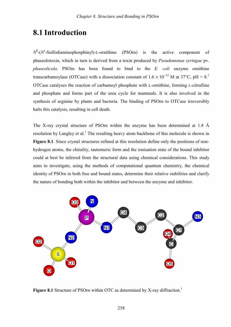
Chapter 8. Structure and Bonding in PSOrn
258
8.1 Introduction
Nδ-(N′-Sulfodiaminophosphinyl)-L-ornithine (PSOrn) is the active component of
phaseolotoxin, which in turn is derived from a toxin produced by Pseudomonas syringae pv.
phaseolicola. PSOrn has been found to bind to the E. coli enzyme ornithine
transcarbamoylase (OTCase) with a dissociation constant of 1.6 × 10⁻¹² M at 37°C, pH = 8.1
OTCase catalyses the reaction of carbamoyl phosphate with L-ornithine, forming L-citrulline
and phosphate and forms part of the urea cycle for mammals. It is also involved in the
synthesis of arginine by plants and bacteria. The binding of PSOrn to OTCase irreversibly
halts this catalysis, resulting in cell death.
The X-ray crystal structure of PSOrn within the enzyme has been determined at 1.8 Å
resolution by Langley et al.1 The resulting heavy atom backbone of this molecule is shown in
Figure 8.1. Since crystal structures refined at this resolution define only the positions of non-
hydrogen atoms, the chirality, tautomeric form and the ionisation state of the bound inhibitor
could at best be inferred from the structural data using chemical considerations. This study
aims to investigate, using the methods of computational quantum chemistry, the chemical
identity of PSOrn in both free and bound states, determine their relative stabilities and clarify
the nature of bonding both within the inhibitor and between the enzyme and inhibitor.
����������
�������������
�����������������
����������������������
���������������
���������������
�����
�������������
�������������
�������������
������������� �����
���������������
���������������
���������������
���������������
���� ���������������
�����������
�����������
��������������
��������������
��������������
��������������
�����������������
��������������
�������������������
�������
�������
���������
������������
���������������
�
������������
������������
����������������
������������
������������
������������
������
����������������
����������������
����������������
�����
������������
����������������
����������������
����������������
��������������������
�������������
�������������
��
O
N2
C
S
N
N1
P
O2
O3
O1
O4
C2 N3
O5
C1 C3
C4
Figure 8.1 Structure of PSOrn within OTC as determined by X-ray diffraction.1

Chapter 8. Structure and Bonding in PSOrn
259
Langley et al.1 proposed that PSOrn acts as a transition state analogue within the enzyme; that
is, it adopts the same conformation and forms the same type of hydrogen bonds with the
enzyme as in the suggested carbamoyl phosphate + L-ornithine transition state. They
examined the self-consistency of possible hydrogen bonding networks at the enzyme active
site and concluded that the most likely chemical form of the bound inhibitor is a doubly
ionised “imino” tautomer and that the phosphotriamide is the R enantiomer as shown in
Figure 8.2 (along with the substrates, proposed transition states and a more conventional
amino form of the inhibitor). The observed potent inhibitory activity of PSOrn could thus be
rationalised because this species is a structural mimic of the substrates in a proposed transition
state.
Figure 8.2 Imino and amino tautomers of PSOrn as transition state analogues for the OTC
catalysed reaction, as proposed by Langley et al.1
Conventional chemical wisdom suggests that free PSOrn would be more stable in the amino
form, that is, with the P-N-S nitrogen protonated. Moreover, such protonation would not
necessarily preclude hydrogen bond donation to this nitrogen, given the presence of a lone
pair on N. The current investigations were undertaken with the primary aim of elucidating the
nature of the interaction between PSOrn and some of the important enzyme residues, in
particular the hydrogen bonding of an arginine to the P-N-S nitrogen of the inhibitor. To
reduce computational costs the (CH2)3CH(NH3+)(CO2
−) side-chain of PSOrn has been
replaced by a methyl group. The relative stabilities of several tautomeric amino and imino
forms of the resulting neutral model compound are investigated by density functional theory,
NH3+
C
(CH2)3
N HH
CH2N
OO
P
O-
O-
O
NH3+
C
(CH2)3
N+ HH
CH2N
O-O
P
O-
O-
O
NH3+
C
(CH2)3
N H
PH2N
ON
S
O
O-
O
Substrates for ReactionCatalysed by OTC
Proposed TransitionState
Proposed IminoStructure for
Phaseolotoxin
CO2-H CO2
-H H CO2-
NH3+
C
(CH2)3
N H
PH2N
ONH
S
O
O-
O
Proposed AminoStructure for
Phaseolotoxin
H CO2-
-

Chapter 8. Structure and Bonding in PSOrn
260
followed by similar studies on adducts of these with one and two (model) arginine molecules.
In addition to providing information on the relative stabilities of the amino and imino forms of
the inhibitor in both free and bound forms, these studies also yield charge distribution data
and thus some insight into the nature of bonding within the inhibitor as well as between
inhibitor and enzyme.
8.2 Methods
In the work reported in this chapter neutral PSOrn is represented by model compound,
denoted PSO, obtained by the replacement of the (CH2)3CH(NH3+)(CO2
−) side-chain of
PSOrn by a methyl group. The structure of an amino form of PSO is shown schematically in
Figure 8.3. As indicated by the X-ray data, the side-chain is not directly involved in the
binding of PSOrn to the arginine residues. Therefore, the above simplification of the inhibitor
is not expected to significantly affect the inhibitor/arginine interactions, especially since the
CH(NH3+)(CO2
−) group, being at the end of a fully extended saturated alkyl chain, would only
marginally affect the covalent bonding pattern (and hence electron density) within the
“active” PSO moiety (either via through-space or through-bond interactions).
Figure 8.3 The structure (connectivity) of PSO, the model compound for PSOrn.
The quantum chemical calculations on PSO and the PSO/arginine adducts were carried out
using density functional theory (see Section 2.3), utilising the B3LYP exchange-correlation
hybrid functional2-4 and the 6-31G(d) basis set. Full geometry optimisations were performed
as well as constrained optimisations, where only the hydrogen coordinates were allowed to
relax while the heavy atom coordinates were constrained at the X-ray values. For a number of
CH3
NH
PH2N
ONH
S
O
OHO

Chapter 8. Structure and Bonding in PSOrn
261
species the energies were recalculated using the fully polarised 6-31G(d,p) basis. The
inclusion of polarisation functions on the hydrogens resulted in effectively negligible changes
in the relative energies. Due to computer resource limitations vibrational frequencies and
hence zero point energy (ZPE) corrections were not, in general, computed. On the basis of
ZPE computations on the Zw1 and Zw2 dimers and their constituent PSO and arginine
monomers, the dissociation energy of a dimer would be reduced by ~ 5 - 10 kJ mol−1, viz. up
to ~ 15%, by the inclusion of ZPE. As this work does not aim to produce energies of chemical
accuracy, the omission of ZPE is justifiable.
All calculations were carried out using the Gaussian98 programs5 on DEC alpha 600/5/333
and COMPAQ XP1000/500 workstations of the Theoretical Chemistry group at the
University of Sydney and the 64 processor SGI Origin 2400 of the Australian Centre for
Advanced Computing and Communications (ac3).
8.3 Results and Discussion
8.3.1 Free (Model) Inhibitor
All chemically reasonable tautomers of the model inhibitor PSO were considered in an effort
to locate the most stable tautomer and to quantify their relative stabilities. Free PSO, and thus
PSOrn, has the potential to form intramolecular hydrogen bonds which, in all probability, will
have a considerable effect on these stabilities. The optimised structures of five amino and
three imino tautomers of neutral PSO are shown in Figure 8.4 and Figure 8.5, along with
their relative energies. Although it may not be immediately obvious from these figures, the
geometries of the heavy atom backbones of the various tautomers are quite different,
especially in the angles. The variation is attributed, in part at least, to the effects of
intramolecular hydrogen bonding which, of course, are tautomer dependent. Constraining the
heavy atom coordinates to their X-ray values effectively eliminates most of the intramolecular
hydrogen bonds at an energy cost of ~ 400 kJ mol−1. As only part of this energy could be
reasonably attributed to the hydrogen bonds, the relaxation energy associated with
optimisation of the (covalent) bond distances and bond angles is obviously substantial. In
light of such demonstrated sensitivity of the energy to relatively small variations in the

Chapter 8. Structure and Bonding in PSOrn
262
Figure 8.4 Amino tautomers of PSO. (Energies relative to amino1.)
��������
�����
����������
������������
������������
���
����������
����������������
������
�����������
�������������
���������������
���������������
������������������
������
������
��
��������������
��������������
���
������
������������
�����
�����
�����
�����
�����
�����
���������� ����
����������
����������
��������
��������
��������
������������
������������
��������
������������
H
H
H
H
H
H
H
O
H
O O
O
S P N
C
N
N
���� �������
�������
�������
��������������
����������
������
������
���� ���� ��������
�������������
����
��������������
������������
���������������
����
����������������
�������������������� ����
������������
��
���� �������������
����������
�����
�����
�����
������� ���� ��� �����
�����
�������� ���� ���� ��������
��������
H
H H
H
H
H H
H
O N
C
S
N
N
P
O
O
O
�������
�������
�����
�����
���������
����������
������������
���������������
�������
�����
�����
�����
���� ���
�����������
�������������
�������������
�������������
������
������
���������������������
������������������������
�������
�������������
����
������
������
��������
�������������
�������������
����
����
������
������
�������� ���
�����
����
����
���������
������������
�������
��������
�������
�������
���������� ��� ���
�����
�����
H
H
H
H
H
H
H
H
O
N
C
S
N
N
P
O
O
O
������
��������������
������
��������
����������
����������
������������ ��
������
�����������
��������
�����������
�
���������������
����������������
������
������
������
�����
��������������
����
�������������������
���
�����������
��������������
������
������
������
�����
�����
����������
������
������
������ ��
������
������
�������� �����
���������
H
H
H H
H
H
H
H
O N
C
S
N
N
P
O
O
O
�����������
�����������
������
�����
�����
�����
����������
�������
����������
��������������
��������
�����
������
������
������
��� ���
���������������
���������������
�� ��
��������������
��������������
�����������������
���������
����
����
��������
������
������
������
����
��� ��� �����
����������
����������
������������ ��
�����������
��������
�����������
��������������
������
������H
H
H H
H
H H
H O
N
C
S
N
N P
O O
O
Amino1: E = 0.0 kJ mol−1 Amino2: E = 8.9 kJ mol−1
Amino3: E = 19.1 kJ mol−1 Amino4: E = 22.8 kJ mol−1
Amino5: E = 37.5 kJ mol−1

Chapter 8. Structure and Bonding in PSOrn
263
Figure 8.5 Imino tautomers of PSO. (Energies relative to amino1.)
geometry, there is clearly a need for fully relaxed calculations; i.e., we cannot rely entirely on
the results of constrained computations.
According to the computed equilibrium energies listed in Figure 8.4 and 8.5 the imino
tautomers are substantially less stable than the amino forms. This was expected, as in the
former the S−N−P nitrogen would have two lone pairs of electrons and a formal negative
charge; to stabilise such a structure considerable charge delocalisation would be needed. As
will be shown later (Section 8.3.3), the sulfur and phosphorus atoms in their respective
������
����������
��� ��� ������ ���
�������
�������
��� �������
�������
���������
���������
���������
�����������
�
��������������
���������
���������
�����
�����
�������������
��
��������������������
�������������
���
�����
�����
�����
�����
��������
�������������
������
������
������
������
���������� �������
�����
�����
�����
�����
�����
������
������
�����
�����������
H
H
H
O H
H
H
H
H
O
O O N
C
S
N
N
P
�������������
����������
���
�����
�����
�����
�����
���������
���������
���������
�����
������
������
������������
������������
�����������
�������������� ���
�������
�������
�������
�����
�����
��������������
��������������
� �������������������
������������������
���� ����
���������
������
�����������
�������
�������
�������
������
������ ��� ��� ������ ����
������������
��������
�����
����������
������������
�������
H
H
H
O
H
H
H
H H
O
O
O
N
C
S
N
N P
����������
������������
�����������
����
������
������
�����
�������
������������
�������
�������
����������
�����������
��������������
�����
������������������
�������
�������
�������
������
���������������
����
�������������������
���
�����������
���������������
����
����
������� ��� ��� ����� ���
�����
����
����
��� ��� �����������������
�������������� ���H
H
H H
H
H
H
H
O N
C
S
N
N P
O
O
O
Imino1: E = 52.3 kJ mol−1
Imino3: E = 125.6 kJ mol−1
Imino2: E = 75.4 kJ mol−1

Chapter 8. Structure and Bonding in PSOrn
264
environments in PSO cannot participate in π bonding to any appreciable degree; that is, no
significant π charge delocalisation occurs. This is contrary to the implications of the Lewis
structure of the imino form of PSOrn in Figure 8.2. Hence the marked difference in stabilities
between amino and imino tautomers.
8.3.2 Bound (Model) Inhibitor
The crystal structure of PSOrn in OTCase indicates that the inhibitor is hydrogen bonded to
an arginine residue (Arg57), as shown in Figure 8.6. In particular, the distance of 2.79 Å
between the S−N−P nitrogen (N2) and the C−N−C nitrogen (NArg) of the arginine residue
suggests a strong hydrogen bond mediated N…N interaction, as noted by Langley et al.1
However, the N2…NArg interaction may be expected to be destabilising in the case of an
amino tautomer, since the near-planar arrangement of the S−N2−P and C−NArg−C groups
would imply that the N2−H and NArg−H groups would be pointing towards each other, which
would result in strong repulsion between the hydrogens.
Figure 8.6 X-ray structure of PSOrn fragment with Arg57 residue.
�������
����������
����������
���������� ��
����������
��������������
��������������
������
�������
�������
�������
������
����������
����������
�������
���������
�����������
�����������
�������������� ���
���������������
���������������
���������������
�����������
��������������������
��������
��������
������������
�����������
�����������
��������������
2.79 Å
N2
O N
CA
S P
O
O O
C
N
NArg
3.04 Å
CA1
NA1
NA2

Chapter 8. Structure and Bonding in PSOrn
265
As this interaction is expected to have the most significant effect on the relative stabilities of
the tautomers, it was studied in some detail. Two approaches were used: (a) full optimisation
of the geometry (relaxed calculation) and (b) partial optimisation, where the heavy atom
backbone is constrained at the X-ray geometry and only the hydrogen positions are optimised
(unrelaxed calculation). The first approach has the advantage of yielding optimal geometries,
including hydrogen bond distances, and interaction energies. However, the strong
intramolecular hydrogen bonds in the inhibitor, as discussed in the previous section, could
considerably deform the structure, thus making comparisons between the computed
equilibrium geometries and the X-ray values effectively meaningless. (In reality the enzyme
bound PSOrn forms intermolecular hydrogen bonds to the various residues around it in
preference to intramolecular hydrogen bonds.) To simplify the calculations only the
interaction between PSO and a truncated form of the arginine residue (C2N3H7), as shown in
Figure 8.6, was studied.
Initially the range of PSO-arginine adducts that were studied were hydrogen bonded
complexes of the various (amino and imino) tautomers of PSO (as shown in Figure 8.4 and
8.5) and neutral arginine, i.e., dimers. The lowest energy dimer in this group is a complex
involving the amino1 tautomer, with binding energies computed as 27.5 and 11.3 kJ mol−1
from the relaxed and unrelaxed calculations respectively. This suggests that the N2…NArg
interaction is stabilising, although the N2…NArg distance is considerably longer than in the X-
ray structure. As can be seen from the structure in Figure 8.7, in the complex the arginine
moiety is distorted, with the NArg−H bond rotated out of the molecular plane. The interaction
of the imino1 tautomer with arginine gives rise to considerably larger binding energies: 50.9
and 26.8 kJ mol−1 from the relaxed and unrelaxed calculations respectively. Nevertheless, in
absolute terms the amino1-arginine complex is more stable by ~ 29 kJ mol−1, as indicated by
the relaxed calculations.
On extending the calculations to zwitterionic dimers, that is, complexes of deprotonated PSO
(denoted PSO−) and protonated arginine, it was found that two of these are more stable, even
in gas phase, than the dimers between neutral partners. The structures of these complexes
(denoted Zw1 and Zw2) are also shown in Figure 8.7. The PSO− moieties in both of these
dimers are imino tautomers. As can be seen from the tabulated distances in Table 8.1, the

Chapter 8. Structure and Bonding in PSOrn
266
Figure 8.7 Structures of the three most stable PSO…Arg dimers.
���������
���������
��� ���
�������
���������� ���
���������
���������
������
��������
��������
������
������
��������
������������
�������� ���
���������������
���������������
���
���������
���������
�����
���������
���������
��������������
������
������
����������
����������
�����
�������
����������
����������
����������
����������
����
����
���������
���������
�����
���������
�������������
��������������
��������
��������
��������
����
����
�������������
�������������
�����
���������
����������
����������
����������
����������
��������������
��������
������
������������
����������������
�������
�������
��������
������������
���� ��������� ��
����������������
�������
�������
�����
�����
H
H
H
H
H H
H
O N
C
S
N
N
P O
O
O
C
C
H
H H
H H
H H
N
N
2.74 Å 2.79 Å
H N
PSO−(Imino)…ArgH+ (Zw1)Dimer
PSO−(Imino)…ArgH+ (Zw2)Dimer
PSO(Amino1)…Arg Dimer
��������
�����������
�����
��������
��������
��������
�������
�������
��������������
����������������
��� ���
���������
��� ���
�������
�������
�������
�������
�������
�������
����������
��������
������������
���� ����
��������
��������
��������
���������
���������
���������
������������
����������
����������
���������
���������
����
��������
��������
��
����������
�������������
���������
���������
�������������
������
������������������
����������
����������
�
��������
������������ ����
������������
������������
������������
����������
����������
������������
���� ������
�������
�������
�����
�����
��������
�����
H
H
H
H
H
H H
H
O N
C
S
N
N
P
O
O
O
C
C
H
H
H
H H
H H
N
N
2.81 Å 2.79 Å
N
����������
��������
����������������
�������
�������
�������
����
�����������
��������������
�����
���������
���������
���������
�����
���������
�������������������
��������
������
������
���������� ����
����������
�������
����
�������������
�������������
�������������
�����
��������
�����
��������
������������
����������
����������
����������
�����
�����
������������������
������
��������
�������������
�������������
�����
�����
����������
����������
���� ����
��������
������������ ����
������
������
������
������
������
������
���������
���������
���������
�����
�����
������
������
������
����
���� ����
������
�����
�����
���������
���������
���������
�����
�����
������������ ����
������������� ���
����������
H
H
H H
H
H
H
H
O N
C
S
N
N
P
O
O
O
C
C
H
H
H H
H
H
N
N
2.81 Å 2.79 Å
N
H

Chapter 8. Structure and Bonding in PSOrn
267
Table 8.1. Selected X-ray distances for enzyme bound PSOrn and corresponding computed
distances in PSO…Arg dimers and PSO…(Arg)2 trimer.a
Atom-Atom Distance /Å
Bound PSOrnX-ray
PSO…Arg(Zw1)
PSO…Arg(Zw2)
PSO…(Arg)2
Trimer
S−O 1.51 1.48 1.49 1.50
S−O1 1.34 1.63 1.50 1.52
S−O2 1.58 1.46 1.48 1.49
S−N2 1.60 1.62 1.69 1.65
N2−P 1.66 1.65 1.59 1.63
P−O3 1.48 1.49 1.49 1.52
P−N 1.72 1.71 1.69 1.71
P−N1 1.61 1.74 1.89 1.70
N1−C 1.48 1.47 1.49 1.47
N2−NArg 2.79 2.81 2.74 2.72
O−NA1 3.04 2.76 2.76 2.70
CA−NArg 1.46 1.46 1.45 1.45
NArg−CA1 1.33 1.32 1.32 1.32
CA1−NA2 1.33 1.36 1.37 1.37
CA1−NA1 1.33 1.34 1.34 1.34
O1−Na1 2.76 2.72
O3−Na2 2.73 2.69
Ca−Na 1.45 1.47
Na−Ca1 1.33 1.36
Ca1−Na1 1.32 1.34
Ca1−Na2 1.32 1.34
a Labelling of atoms as indicated in Figure 8.1.
Subscripts Arg, A, A1, A2 refer to atoms of Arg57 (See Figure 8.6).
Subscripts a, a1, a2 refer to atoms of Arg106.
fully optimised geometry of Zw1 matches the X-ray data reasonably well. Agreement
between theory and experiment is less convincing in the case of Zw2, where the P−N1 bond
distance of 1.89 Å is clearly at variance with the X-ray value of 1.61 Å. Zw2, however,
appears to be the more stable (by 13.2 kJ mol−1) of the two dimers. Compared with the lowest
energy amino1-arginine complex, Zw1 and Zw2 were computed to be 24.0 and 37.2 kJ mol−1
more stable respectively, corresponding to binding energies of 51.5 and 64.7 kJ mol−1 with

Chapter 8. Structure and Bonding in PSOrn
268
respect to neutral arginine and the amino1 form of PSO. The stabilities of the various dimers,
as well as of a trimer (as discussed below), are summarised in Table 8.2 as dissociation
energies to a range of neutral and charged moieties.
Table 8.2 Computed dissociation energies of PSO…Arg dimers and trimers.
∆E /kJ mol−1
PSO(Amino1) … Arg Dimer → PSO(Amino1) + Arg −−27.5
PSO(Imino1) … Arg Dimer → PSO(Amino1) + Arg −−−1.3
PSO(Imino1) … Arg Dimer → PSO(Imino1) + Arg −−50.9
PSO− (Imino) … ArgH+ Dimer (Zw1) → PSO(Amino1) + Arg −−51.5
PSO− (Imino) … ArgH+ Dimer (Zw1) → PSO− (Imino) + ArgH+ −332.8
PSO− (Imino) … ArgH+ Dimer (Zw2) → PSO(Amino1) + Arg −−64.7
PSO− (Amino) … ArgH+ Dimer (Zw3) → PSO(Amino1) + Arg −126.5
PSO2− (Imino) … (ArgH+)2 Trimer → PSO(Amino1) + 2 Arg −170.8
PSO2− (Imino) … (ArgH+)2 Trimer → PSO− … ArgH+ Dimer (Zw1) + Arg −119.3
PSO2− (Imino) … (ArgH+)2 Trimer → PSO2− + 2 ArgH+ 1284.2
The relative stabilities of PSO and PSO…Arg dimers, as obtained in constrained and relaxed
calculations are shown in Figure 8.8. The trends in the stabilities appear to be qualitatively
reproduced by the constrained optimisations, but clearly the energy differences, especially
between the PSO(Amino1)…Arg dimer and Zw1, are predicted to be considerably larger by
the constrained calculations. As remarked in the previous section, in light of the large energy
differences between the unrelaxed and relaxed structures, we regard the latter as the more
reliable.
Interactions between amino tautomers of PSO− and protonated arginine (denoted ArgH+) were
found to be repulsive, as expected. Although in the latter complexes ArgH+ did bind to PSO−,
this did not occur via N2, as would be required for a valid description of the binding of PSOrn
in the enzyme.

Chapter 8. Structure and Bonding in PSOrn
269
Figure 8.8 Relative energies (in kJ mol−1) of PSO tautomers and PSO…Arg dimers from
constrained and relaxed calculations.
According to the X-ray data, PSOrn interacts with two arginine residues, the second (Arg106)
effectively bridging the O1 and O3 atoms of PSOrn (see Figure 8.1). A trimer of PSO with
two arginines is clearly a more realistic model for the binding of PSOrn to the enzyme. Given
the apparent propensity of arginine to exist in protonated form, our trimer calculations were
restricted to a complex of a (doubly deprotonated) dinegative PSO (denoted PSO2−) and two
ArgH+ subunits. The computed structure of this trimer is shown in Figure 8.9. The key
interatomic distances are listed in Table 8.1. The agreement with the X-ray data is good,
given the relatively high estimated errors of ± 0.2 Å in the X-ray distances. The large binding
energy of 170.8 kJ mol−1, relative to neutral PSO and two arginines, is consistent with the
action of PSOrn as an effective inhibitor that binds irreversibly to the enzyme.
PSO (Amino1)…Arg Dimer
PSO (Imino1)…Arg Dimer
PSO− (Imino)…ArgH+ Dimer (Zw1)
PSO− (Imino)…ArgH+ Dimer (Zw2)
−390.9
52.7
−466.2
0.0
28.8 24.0
−482.5
−453.7
0.0
37.0
−506.5
−100.2
−519.713.2
75.4Relaxed
Unrelaxed
PSO PSO…Arg Dimers

Chapter 8. Structure and Bonding in PSOrn
270
������
����������
�����
�����
��� ��� ������ �����
�����
����� ����
����������
����������
���� ����
���������
��������������
�������
�������
�������
�������
������������
�������
�������
�����
�����
��������
��������
������������ ����
����������
������������
����������������
�����
�����
���������������
�������������
�������������
�������������
������
����������
����������
����������
����������
����������������
���������������
������������������
���������
���������
�������
�������
��
��� ��������������������
��������������
������
����������
�������� ��H
H
H
ON
S
N
PO
OO
C
H
H
H
H
H
H
H
H
H
H
N
NC
NNC
H
2.75 Å
2.74 Å
H
Figure 8.9 Structures of PSO…(Arg)2 trimer and PSO…Arg (Zw3) dimer.
��������
������
������
���������
����
����
����
����
����
����
�������
�������
������������������������
������
������
�������� ��
�����
�����
������
������
�����
�������
�������
������������
������������
������������
����������
����������
���������
���������
���������
��������
��������
�����
������
�����
����������
���������
�������������
�������������
�����
�������
�������
�������������
�������������
�����������
�����������
�����������
������
������������
����������������
������
��������
��������
������
���������
������������
������������
����������������
��������
��������
������������
���������������
����������������������
�����
����������
����������
������������
������������ ����
����
�������
�������
�������
�������
��������������
��������
����������
����������������
����������
�������
����������
Arg57+
Arg106+
PSO2-
H
H H
O
S N
P
O
O O C
H
H
H
H
H
H
H
H H
H
C C H
2.72 Å
2.69 Å
H
H
H
H
H
H
H H
C C
2.72 Å 2.70 Å
N
N
N N
N
N
N N
Chapter 8. Structure and Bonding in PSOrn
271
The very much higher stability of the trimer (to dissociation) than of the dimers Zw1 and Zw2
suggests that the interaction between a PSO− ion and ArgH+ (representing the Arg106 residue)
is actually the dominant contribution to the overall stability, rather than the interaction with
the (protonated) Arg57 residue. To test this hypothesis the structure of a third zwitterionic
dimer (Zw3) was optimised. This derives from the trimer by the removal of neutral Arg57
(See Figure 8.9). PSO− in Zw3 was chosen to be an amino tautomer. According to the
calculations Zw3 is more than twice as stable as Zw1, its dissociation energy to PSO and Arg
having been computed to be 126.0 kJ mol−1. Thus the overall binding energy of the trimer is,
to a good approximation, the sum of the individual binding energies to the two arginine
residues.
In the zwitterionic dimers, as well as in the trimer discussed above, the overall binding
between the negatively charged PSO− and ArgH+ moieties, in addition to the hydrogen
bonding, has a substantial ionic (electrostatic) contribution. This can be quantified through the
analysis of the binding energies of Zw1, Zw2 and the trimer, relative to neutral PSO and Arg
as well as relative to the ions PSO−, PSO2− and ArgH+. These results are included in Table
8.2. Thus Zw1 and Zw2 are bound by nearly 350 kJ mol−1 relative to the ions, but because of
the very different proton affinities of PSO− and Arg, the binding energies relative to the most
stable amino tautomer of PSO and Arg are nearly an order of magnitude smaller.
Furthermore, the PSO2−…(ArgH+)2 trimer is bound by 1284 kJ mol−1 relative to the ions.
8.3.3 Charge Distribution and Bonding
In Figure 8.2, following the usual convention, the Lewis structures of amino and imino
tautomers of PSOrn were drawn with several PO and SO double bonds, with the implication
that P and S are hypervalent; that is, they accommodate more than eight electrons in their
valence shells. In the case of the P=O and S=O bonds this implies utilisation of the 3d atomic
orbitals of P and S in the formation of the appropriate P-O and S-O π molecular orbitals. The
validity of such “expansion of the octet” has been strongly debated in the literature over the
past 20 years.6-9 On the basis of careful quantum chemical studies several authors have
concluded that the electronic structures of molecules with apparently hypervalent multiply
bonded second row atoms are best described by invoking semipolar bonds, where, for

Chapter 8. Structure and Bonding in PSOrn
272
example, the P and S atoms acquire formal charges of up to +2, which then allows these
atoms to form up to four covalent bonds with O− (or other atoms or ions)6,7,9,10. The semipolar
bonds thus have both covalent and ionic components and are comparable in strength with
double bonds, with bond lengths to match.
In light of the above observations, the amino structure of PSOrn in Figure 8.2 would be more
correctly drawn by replacing each P=O and S=O with P+− O− and S+− O− semipolar bonds
(which would result in S with a formal 2+ charge), as shown in Figure 8.10. The imino
tautomer, however, as drawn in Figure 8.2, relies on π resonance to partially delocalise the
negative charge on the PNS nitrogen due to the two lone pairs. Thus, if P and S cannot
participate in π bonding, the above mechanism for charge delocalisation cannot be invoked.
Hence our initial suspicion that amino forms of PSO would be considerably more stable than
any imino tautomer. In the case of isolated PSO these suspicions proved well-founded as the
computations located five amino type tautomers which were more stable than the lowest
energy imino tautomer (Figures 8.4 and 8.5).
Figure 8.10 Lewis structure of an amino tautomer of PSOrn with semipolar bonds.
NH3+
C
(CH2)3
N H
P+
H2NO-
NH
S++
O-
O-
O-
H CO2-

Chapter 8. Structure and Bonding in PSOrn
273
8.3.3.1 Population Analysis
As in previous studies which have addressed the problem of hypervalency, we have used the
Roby-Davidson (RD) method11-14 (with the B3LYP/6-31G(d) density matrix) to carry out
population analyses on free as well as bound PSO, yielding atomic charges and shared
electron numbers (σ) for pairs of atoms. The latter is interpreted as a direct measure of the
covalent character of a given bond. It must be noted, however, that shared electron numbers
are not bond orders and thus their interpretation requires calibration. This was carried out by
analysing the shared electron numbers of a range of small molecules (H2PNH2, PO(NH2)3,
H3PNH, HPNH, HPO, HOPO, H3PO, HSNH2, H2SNH, SNH, HSOH, H2SO4, H3SO, SO) and
correlating the shared electron numbers with bond lengths and bond orders, provided the latter
could be reasonably assigned, for example double bonds in S=O and HP=O, and single bonds
in H2P−NH2 and HS−NH2. Thus, as shown in Table 8.3, for PN and PO: σ = 1.0 - 1.22 are
consistent with single bonds, σ = 1.76 - 1.83 describe double bonds, while σ = 1.40 - 1.50
apply to semipolar bonds. Lower σ values describe such bonds in the case of SN and SO
linkages. Atomic charges can also be calibrated, with Nq or Oq values of ~ −0.25 to ~ −0.5
being consistent with single or double bonds and ~ −0.6 to ~ −0.75 consistent with semipolar
bonding. Pq and Sq show greater variation with the nature of their bonding partners, in
general, however, q = 0.1 to 0.5 indicate single or double bonds whereas q > 0.6 (with only
one N or O partner) indicate the presence of a semipolar bond. Bonding to additional N or O
atoms increases Pq or Sq such that S in H2SO4 (with two single and two semipolar SO bonds)
has a charge of 1.87. As noted earlier, this calibration shows that it is not possible to
distinguish between double and semipolar bonds on the basis of bond lengths (which may
have led to the original assumption that semipolar bonds were π bonds); semipolar bonds can
be identified, however, by the lower values of σ and the higher atomic charges.
The computed shared electron numbers and atomic charges for the amino1 and imino1
tautomers of PSO, along with those of the zwitterionic dimer Zw1 are listed in Table 8.4 and
Table 8.5. Almost all the bonds between the heavy atoms of PSO are described as single or
semipolar bonds. A partial double bond character has been assigned to the P−N2 bond in the
imino1 tautomer of PSO. In this molecule, due to the protonation of N1, the P−N1 bond is
long and weak and therefore a degree of bonding π interaction between the P and N2 atoms is
possible. The high positive charges on the S and P atoms along with the high negative charges

Chapter 8. Structure and B
onding in PSO
rn
274
Table 8.3 Calibration of Roby-Davidson population analysis results (shared electron populations and atomic charges) along with bond lengths
for P-N, P-O, S-N and S-O single, double and semipolar bonds.
P−N P−O
Molecule RPN /Å σ qP qN Molecule RPO /Å σ qP qO
Single Bond H2PNH2 1.73 1.22 0.24 −0.44 H2POH 1.68 1.04 0.33 −0.44
PO(NH2)3 1.69 1.01 1.30 −0.53 HOPO 1.64 1.00 0.64 −0.45
Semipolar Bond H3PNH 1.57 1.50 0.79 −0.66 H3PO 1.49 1.41 0.87 −0.60
PO(NH2)3 1.50 1.39 1.30 −0.66
Double Bond HPNH 1.59 1.83 0.30 −0.37 HOPO 1.48 1.75 0.64 −0.41
HPO 1.50 1.75 0.50 −0.37
S−N S−O
Molecule RSN /Å σ qS qN Molecule RSO /Å σ qS qO
Single Bond HSNH2 1.72 0.85 0.13 −0.41 HSOH 1.70 0.91 0.20 −0.41
H2SO4 1.63 0.76 1.87 −0.51
Semipolar Bond H2SNH 1.61 1.25 0.64 −0.70 H3SO 1.49 1.19 1.06 −0.72
H2SO4 1.45 1.21 1.87 −0.65
Double Bond SNH 1.58 1.64 0.13 −0.26 SO 1.52 1.47 0.31 −0.31
274

Chapter 8. Structure and Bonding in PSOrn
275
Table 8.4 Selected bond lengths (R in Å), Roby-Davidson shared electron numbers (σ in e)
and assigned bond types of amino and imino tautomers of PSO and of the PSO…Arg dimer
(Zw1)a
PSO (Amino1) PSO (Imino1) PSO…Arg Dimer (Zw1)
R σ Bond Type R σ Bond Type R σ Bond Type
S−O 1.45 1.3 Semipolar 1.63 b 0.8 Semipolar 1.48 1.1 Semipolar
S−O1 1.46 1.2 Semipolar 1.47 1.2 Semipolar 1.63 b 0.8 Semipolar
S−O2 1.61 b 0.8 Single 1.48 1.1 Single 1.46 1.2 Single
S−N2 1.70 0.9 Single 1.61 1.1 Part. Double 1.62 1.1 Single
P−N2 1.72 1.0 Single 1.60 1.3 Single 1.65 1.1 Single
P−O3 1.50 1.3 Semipolar 1.48 1.5 Semipolar 1.49 1.4 Semipolar
P−N 1.66 1.1 Single 1.67 1.1 Single 1.71 1.0 Single
P−N1 1.67 1.1 Single 1.92 0.6 Weak Single 1.74 0.9 Single
a Labelling of atoms as indicated in Figure 8.1.b Part of SOH group.
Table 8.5 Atomic charges (in e) on heavy atoms for PSO in amino and imino tautomers of
PSO and of the PSO…Arg dimer (Zw1) from Roby-Davidson analysis.a
PSO(Amino1)
PSO(Imino1)
PSO…Arg Dimer(Zw1)
S 1.79 1.77 1.84
O −0.72 −0.46b −0.82
O1 −0.59 −0.81 −0.59b
O2 −0.53b −0.64 −0.74
N2 −0.82 −1.08 −1.19
P 1.32 1.27 1.05
O3 −0.89 −0.78 −0.76
N −0.56 −0.62 −0.46
N1 −0.54 −0.28 −0.33
a Labelling of atoms as indicated in Figure 8.1.b Part of SOH group.

Chapter 8. Structure and Bonding in PSOrn
276
on the oxygens of PSO are consistent with semipolar S-O and P-O bonds. The high negative
charge on N2 is according to expectations in the case of imino tautomers, although it is quite
high in the amino1 form as well, due to the polar N-S, N-P, and especially N-H bonds.
Interestingly, there is an increased negative charge localisation on N2 in the case of the Zw1
dimer. This is probably due to the polarisation of PSO by the Arg+ residue.
The population analyses for the amino1 and imino2 tautomers were repeated with basis sets
containing two additional sets of d functions on the P and S atoms (with exponents chosen as
1/3 and 1/9 of those in the 6-31G(d) sets). This was done to ensure that the description of the
atomic 3d orbitals on these atoms is sufficiently accurate and flexible to resolve any incipient
π bonding. No significant changes in charges, shared electron numbers or relative energies
occurred. We conclude therefore that no appreciable π bonding is present in the various
tautomers of PSO and its complexes.
8.3.3.2 Hydrogen Bonding
A related issue is the hydrogen bonding potential of the various terminal oxygen and nitrogen
atoms in PSO. The traditional explanation of hydrogen bonding is that the protonic hydrogen
of the proton donor seeks out regions of high electron density, which are generally provided
by the lone pairs of the proton acceptor. As hydrogen bonds are usually (near) linear, it is
assumed that in general each lone pair is only capable of forming one hydrogen bond. It
would therefore be expected that a doubly bound oxygen atom, formally having two lone
pairs, would be able to form two hydrogen bonds. On the other hand, an oxygen atom
involved in a semipolar bond formally has three lone pairs and would therefore have the
potential to form three hydrogen bonds. The net effect of three lone pairs of electrons is an
effectively uniform (directionless) charge distribution on the oxygen atom. It is therefore
possible that this, coupled with the large negative charges, Oq , for oxygens involved in
semipolar bonding (as shown in Table 8.3) may allow the formation of more than three
hydrogen bonds.
The validity, or otherwise, of this view of hydrogen bonding is particularly important when
attempting to postulate and interpret which enzyme-inhibitor interactions in the crystal

Chapter 8. Structure and Bonding in PSOrn
277
structure of Langley et al.1 involve hydrogen bonds. Careful analysis of the crystal structure
data indicates that for each of the oxygen atoms attached to S (O, O1 and O2 as defined in
Figure 8.1) there are three potential proton donors with appropriate distances and relative
orientations for the formation of three hydrogen bonds. In addition there are four potential
proton donor residues which are appropriately placed to form hydrogen bonds to O3.
It is therefore important to determine whether it is realistic to assign such a large number of
hydrogen bonds to oxygen atoms in these environments. This section thus presents an
investigation of the stabilisation or destabilisation which is obtained for various model
compounds with a range of hydrogen bonding interactions. These model compounds include
H2CO (as the simplest and best understood example of a doubly bound oxygen atom), HPO
(in order to determine the effect of phosphorus on the hydrogen bonding), H3PO (as a simple
example of an oxygen in a semipolar bond) and PO(NH2)3 (as a model for the O3 oxygen in
PSOrn). Water molecules were used as proton donors where the orientation of these moieties
was fixed so there could be no additional stabilisation due to hydrogen bonds between
adjacent water molecules or to other parts of the model compound (see Figure 8.11). The
hydrogen bonds were also constrained to be linear. All other inter- and intramolecular
parameters were then optimised using MP2/cc-pVDZ, thus allowing the stabilisation energy,
stabE , to be calculated relative to the non-interacting monomers. It was, of course, particularly
important to estimate the possible contribution of basis set superposition error to this
stabilisation energy. This was done using the Boys-Bernardi method (described in Section
2.4.5) for each of the interacting molecules. The sum of the individual counterpoise
corrections was subtracted from stabE to give the counterpoise corrected estimate of the
hydrogen bonding energy, HBE . The successive hydrogen bond energies corresponding to the
introduction of 1, 2, 3 and 4 hydrogen bonding water molecules are presented in Table 8.6.
H2CO and HPO, as typical doubly bonded systems, were expected to have two lone pairs and
form two hydrogen bonds; this expectation is clearly confirmed by the results in Table 8.6. In
the case of H2CO a minimum energy structure was also found with the addition of a third
H2O, however two of the water molecules were within only 70° of each other (rather than
120°) indicating that they were binding to the same lone pair on the H2CO oxygen. Although
this structure was found to be stable by 1.7 kcal mol−1 before the application of counterpoise

Chapter 8. Structure and Bonding in PSOrn
278
Table 8.6 Successive stabilisation energies corresponding to the addition of water molecules
as proton donors to H2CO, HPO, H3PO and PO(NH2)3.
Hydrogen Bonds HBE /kcal mol−1
(H2O molecules) H2CO HPO H3PO PO(NH2)3
1 −3.0 −3.0 −4.7 −6.6
2 −2.3 −2.3 −4.1 −6.4
3 −0.9 − −2.7 −6.2
4 − − −0.0 −2.7
corrections, once superposition errors had been accounted for the tetramer was found to be
unstable by 0.9 kcal mol−1, suggesting that the structure is simply an artefact of the relatively
small cc-pVDZ basis set. In terms of its hydrogen bonding propensity, HPO is very similar to
H2CO, although for HPO no local minimum structure with three waters could be found. Thus
it appears that doubly bonded oxygen atoms will only form two hydrogen bonds and that
these align with the expected orientations of two equivalent localised lone pairs (See Figure
8.11).
H3PO formally has a semipolar P-O bond and, as expected, it can form up to three hydrogen
bonds. Local minima were also found on the PES with four and even five water molecules
apparently hydrogen bonded to the oxygen of H3PO. In both these structures the water
molecules appear evenly distributed around the oxygen atom suggesting that the lone pair
charge distribution is fairly directionless (that is, the lone pairs are not spatially discrete). The
stability of these structures could again be a BSSE artefact, however, as suggested by the
counterpoise corrected energies. For the structure with four water molecules the possibility of
attractive interaction between the water molecules was also investigated, however it was
found that the water-water interactions were, in fact, repulsive by 3.7 kcal mol−1.
Finally, binding to the oxygen atom in the hypothetical molecule PO(NH2)3 was investigated
as a model for the O3 atom (bound to P) in PSOrn. Even with the inclusion of the
counterpoise correction, this model compound is capable of forming four hydrogen bonds
with water molecules. The first three interactions are of comparable strength (and much
stronger than those in H2CO, HPO or H3PO) while the fourth seems significantly weaker
although still binding.

Chapter 8. Structure and Bonding in PSOrn
279
We therefore conclude that up to four hydrogen bonds can be attached to an oxygen atom
which is bound by a semipolar bond; it is therefore reasonable to interpret the crystal structure
of PSOrn as showing up to three hydrogen bonds to O, O1 and O2 and up to four hydrogen
bonds to O3.
Figure 8.11 Most stable hydrogen bonded structures for H2CO, HPO, H3PO and PO(NH2)3.
H2CO.(H2O)2
����������
����������
�������
�������
�������
������������������
��������
��������
��������
���������
���������
������������
������������
HPO.(H2O)2
���������
�������
�������
����������
����������
�����������
����������
����������
����������
�������
�������
���������
H3PO.(H2O)3 PO(NH2)3.(H2O)4
�����������
�����������
���
������
��������
�������
�������
��� ���
����������������
����
����������
����������
������������ ��
����������
������������
����
������ ���
�������
��������������
������������
���������
������������
��������� ���
���������
������������
������
�������������
���������
������������
�����
�����
�����
�����
�����
�������
�������
�������������
������
���������
���������
������
���������
���������
���������
����
��������
�������� ����
����������������
�����
�����������
�������������� ���
��� �������������
��������
�� ��
������
������
�������� ��
�����
�����
�����
�����
�� ���������������
�����

Chapter 8. Structure and Bonding in PSOrn
280
8.4 Conclusion
With the aid of quantum chemistry, viz. density functional theory, the binding of PSOrn to the
enzyme OTCase was investigated and modelled through a study of PSO, a simplified model
for PSOrn, and its interaction with one and two arginine molecules. The PSO…(Arg)2 trimer
was found to be bound by ~ 171 kJ mol−1. Such high stability, due to the presence of four
hydrogen bonds as well as a large ionic interaction between the dinegative PSO2− and
protonated arginines, is consistent with the experimental observation that PSOrn is a powerful
enzyme inhibitor. The calculations confirm the proposals of Langley et al.1, inasmuch as
bound PSOrn is a dinegative imino tautomer. While in the case of free (neutral) PSO the most
stable tautomers were calculated to be amino types, when bound to one or two (protonated)
arginines PSO (as PSO− or PSO2−) is predicted to prefer an imino form. However, as in other
phosphorous and sulfur containing molecules, according to the population analyses that were
carried out the P-N, P-O, S-N and S-O bonds in PSO are generally best described as single or
semipolar bonds.

Chapter 8. Structure and Bonding in PSOrn
281
8.5 References
1. D. B. Langley, M. D. Templeton, B. A. Fields, R. E. Mitchell and C. A. Collyer, J.
Biol. Chem., 2000, 275, 20012.
2. A. D. Becke, Phys. Rev. A, 1988, 38, 3098.
3. C. Lee, W. Yang and R. G. Parr, Phys. Rev. B, 1988, 37, 785.
4. A. D. Becke, J. Chem. Phys., 1993, 98, 5648.
5. M. J. Frisch, G. W. Trucks, H. B. Schlegel, G. E. Scuseria, M. A. Robb, J. R.
Cheeseman, V. G. Zakrzewski, J. A. Montgomery, R. E. Stratmann, J. C. Burant, S.
Dapprich, J. M. Millam, A. D. Daniels, K. N. Kudin, M. C. Strain, O. Farkas, J.
Tomasi, V. Barone, M. Cossi, R. Cammi, B. Mennucci, C. Pomelli, C. Adamo, S.
Clifford, J. Ochterski, G. A. Petersson, P. Y. Ayala, Q. Cui, K. Morokuma, D. K.
Malik, A. D. Rabuk, K. Raghavachari, J. B. Foresman, J. Cioslowski, J. V. Ortiz, B.
B. Stefanov, G. Lui, A. Liashenko, P. Piskorz, I. Komaromi, R. Gomperts, R. L.
Martin, D. J. Fox, T. Keith, M. A. Al-Laham, C. Y. Peng, A. Nanayakkara, C.
Gonzalez, M. Challacombe, P. M. W. Gill, B. G. Johnson, W. Chen, M. W. Wong, J.
L. Andres, M. Head-Gordon, E. S. Replogle and J. A. Pople, Gaussian 98 Revision
A.7, Gaussian, Inc.: Pittsburgh, PA, 1998,
6. A. E. Reed and P. v. R. Schleyer, J. Am. Chem. Soc., 1990, 112, 1434.
7. J. A. Dobado, H. Martínez-García, J. M. Molina and M. R. Sundberg, J. Am. Chem.
Soc., 1999, 121, 3156.
8. K. Jug and E. Fasold, Int. J. Quantum Chem., 1992, 41, 687.
9. W. Kutzelnigg, Angew. Chem. Int. Ed. Engl., 1984, 23, 272.
10. A. P. L. Rendell, G. B. Bacskay and N. S. Hush, J. Am. Chem. Soc., 1988, 110, 8343.
11. E. R. Davidson, J. Chem. Phys., 1967, 46, 3320.
12. K. R. Roby, Mol. Phys., 1974, 27, 81.
13. R. Heinzmann and R. Ahlrichs, Theor. Chim. Acta, 1976, 42, 33.
14. C. Ehrhardt and R. Ahlrichs, Theor. Chim. Acta, 1985, 68, 231.

9 Conclusion
Chapter 9
Conclusion
Chapter 9. Conclusion
283
The major focus of the research work presented in this thesis is the calculation of accurate
thermochemical data, including atomisation energies and heats of formation. Gaussian-3 (G3)
and related methodologies have been found to be particularly useful for this purpose, yielding
chemically accurate heats of formation in most cases, with relatively modest computational
cost. Thus the G3 heats of formation of approximately 120 C1 and C2 fluorocarbons and
oxidised fluorocarbons (along with selected C3 fluorocarbons) were calculated. For the most
part, these showed good agreement with the best available theoretical and experimental
literature data, particularly when G3 was used in conjunction with isodesmic reaction
schemes. For molecules for which the G3 results were found to be in poor agreement with
experiment or for which the experimental values had large uncertainties (e.g., HCCF, FCCF,
CCH, CCF and HCOO), more extensive CCSD(T)/CBS calculations have confirmed the
validity of the G3 results, indicating that the literature values may need to be revised. Two
less computationally expensive approximations to G3 were also proposed: G3MP4(SDQ) and
G3[MP2(Full)]. These methods were found to reliably reproduce the G3 results, with mean
absolute deviations from G3 of ~ 0.4 and ~ 0.5 kcal mol−1 respectively for heats of formation
from atomisation energies. These deviations could be further reduced by the application of
isodesmic reaction schemes.
The G3 method was also successfully applied to the calculation of the heats of formation of
molecules containing third row atoms, in particular CFClBr2, and by extension to the
thermochemistry of its dissociation reactions. As G3 results for bromine containing species
had been previously only reported for very small molecules such as HBr, Br2 and CH3Br, it
was gratifying to find excellent agreement between the experimentally determined 0298f H∆ of
184 ± 5 kJ mol−1 and the G3 value of 188 ± 5 kJ mol−1. This work therefore provided further
evidence for the wide range of applicability of the G3 method. In addition, these results have
also provided valuable aid in the determination of the photolysis mechanism for CFClBr2 at
265 nm. Our calculations have predicted the dissociation energy for the two C-Br bonds to be
equal to the (experimental) energy required to produce the CFCl carbene, thus supporting the
hypothesis that the photolysis proceeds via a triple fragmentation pathway, releasing two Br
atoms, rather than by the concerted elimination of a Br2 molecule.
G3 type methods (including G2, G3, G3X and G3X2) as well as more extensive
CCSD(T)/CBS type calculations were also employed in the calculation of the

Chapter 9. Conclusion
284
thermochemistry of 18 small phosphorus containing compounds (P2, P4, PH, PH2, PH3, P2H2,
P2H4, PO, PO2, PO3, P2O, P2O2, HPO, HPOH, H2POH, H3PO, HOPO and HOPO2). The
CCSD(T)/CBS results are consistent with the available experimental values and, as the
estimated uncertainties are quite small, they constitute the most accurate set of heats of
formation available for these molecules. They are therefore regarded as an excellent
benchmark for the testing of the more approximate G3n methods. The G3 and G3X methods
were found to consistently underestimate the benchmark atomisation energies, on average by
3.6 and 1.8 kcal mol−1 and by up to 6.5 and 5.6 kcal mol−1 respectively for this set of
molecules (excluding P4); G2 is comparable in performance to G3. The G3X2 method was
therefore proposed in an effort to improve the G3X results; G3X2 accounts for a higher
degree of electron correlation in comparison with G3 and G3X and, with the inclusion of
counterpoise corrections for BSSE on the phosphorus atoms in the core-valence correlation
calculations, it does show a modest improvement (with a mean absolute deviation from the
benchmark results of 1.5 kcal mol−1). Further investigation has also revealed that the
approximations underlying the Gaussian-n methods become unreliable for molecules which
involve unusual P-P bonding, such as double bonds (in P2 and P2H2), double and semipolar
bonds (in PPO) or large structural strain (in P4). We therefore recommend great care with the
application of these methods to molecules with bonds between second row elements unless
these are simple, unstrained single bonds.
Accurate thermochemical data, in particular those obtained by CCSD(T)/CBS calculations,
along with similar calculations for transition state structures (with appropriate approximations
for variational transition states) allowed us to reliably predict the kinetics of Twarowski’s
proposed catalytic schemes for H + OH recombination. The application of transition state and
RRKM theory resulted in rate coefficients which are consistent with the results of
experimental and modelling studies, although they are in most cases significantly lower than
Twarowski’s estimated values. At 2000K the rates of both catalytic schemes were found to be
comparable and significantly higher than the uncatalysed recombination; both cycles are
therefore expected to be catalytic at this temperature.
The potential energy surfaces for all possible reactions stemming from the NNH + O
recombination were investigated in detail along the appropriate reaction coordinates at the
B3LYP/6-31G(2df,p) level of theory. This study revealed the presence of several reaction

Chapter 9. Conclusion
285
channels which had not been considered previously (including direct abstraction of H by O
and three product channels via the intermediate ONHN) and yielded improved descriptions of
channels which had hitherto been incompletely characterised (dissociation of cis- and trans-
ONNH into NO + NH). The heats of formation were determined for each of the species
corresponding to stationary points on the PES using both G3X theory and a CCSD(T)/CBS
type scheme. A reasonable level of consistency, corresponding to agreement of ~ 2 kcal mol−1
or better between the two sets of results, was observed. This thermochemical and geometric
data was further utilised to generate rate coefficients for the various reaction channels on the
potential energy surface via (variational) transition state and RRKM theories, thus allowing
the overall rate coefficients and the flux through each channel to be determined. We were
therefore able to conclude that the NNH + O channel is considerably less important in
combustion systems than had been previously believed. This was supported by modelling
studies of two combustion systems in the presence of N2 which yielded good agreement with
experiment when our revised thermochemical and kinetic data was employed.
In a study aimed at modelling the binding of the inhibitor PSOrn to OTCase, the relative
stabilities of various amino and imino tautomers of PSO, a model compound for PSOrn, were
investigated both in the gas phase and when bound to (model) residues from the active site of
OTCase. Gas phase calculations revealed that the amino tautomer is the most stable form of
free (neutral) PSO; in the presence of arginine residues, however, the imino structure becomes
lower in energy, the most stable structure being a doubly deprotonated PSO bound to two
Arg+ residues. Thus when bound to the active site of the enzyme, PSOrn would be expected to
adopt a dinegative imino form. Population analysis and hydrogen bonding studies have
revealed that the intramolecular bonds involving second row atoms are either single or
semipolar in nature and that the terminal oxygen atoms are capable of accommodating up to
four hydrogen bonds.

9
Appendices

Appendix 1
A1-1
Appendix 1: Fluorocarbons Supplementary
Information
A1 A1
Appendix 1.1 Atomic data: G3 energies and heats of formation at 0 K of atoms, and thermal
corrections to enthalpies of elements in their standard states, as used in this work.
E0 (G3) / Eh ∆ f H00/ kcal mol−1 H H298
000−c h / kcal mol−1
H −0.5010 51.63 1.01
C −37.8277 169.98 0.25
O −75.0310 58.99 1.04
F −99.6842 18.47 1.05

Appendix 1
A1-2
Appendix 1.2 C1 Hydrofluorocarbons: Rotational constants, vibrational frequencies (scaled by 0.8929), obtained at MP2(Full)/6-31G(d) and
HF/6-31G(d) levels of theory respectively and the resulting zero point energies and thermal correctionsa to the heats of formation.
Species Rotational Constants (cm−1) Vibrational frequencies (cm−1)ZPE
(kcal mol−1)
∆∆ f H2980
(kcal mol−1)
CH4 5.2850 5.2850 5.2848 1328 1328 1329 1520 1520 2856 26.78 2.39
2947 2949 2952
CH3F 5.2414 0.8490 0.8490 1061 1172 1172 1475 1476 1476 23.78 2.42
2886 2957 2957
CH2F2 1.6481 0.3479 0.3045 510 1106 1123 1164 1259 1464 20.16 2.56
1530 2941 3005
CHF3 0.3408 0.3407 0.1868 491 492 680 1126 1185 1187 15.76 2.78
1414 1414 3036
CF4 0.1883 0.1883 0.1883 422 422 610 610 610 896 10.74 3.08
1315 1315 1315
CH3 9.5909 9.5909 4.7955 275 1375 1375 2933 3090 3090 17.35 2.66
CH2F 8.7668 1.0151 0.9215 770 1133 1143 1443 2962 3088 15.07 2.46
CHF2 2.2359 0.3603 0.3152 521 1041 1150 1181 1343 3005 11.78 2.55
CF3 0.3573 0.3573 0.1850 491 491 677 1086 1286 1286 −7.60 2.77
CH2 20.0859 11.2493 7.2108 1397 2794 2850 10.06 2.37
CHF 15.669 1.2090 1.1224 1189 1405 2727 −7.61 2.39
CF2 2.8441 0.4132 0.3608 651 1155 1240 −4.35 2.48
CH 14.4520 2733 −3.91 2.07
CF 1.3802 1259 −1.80 2.08

Appendix 1
A1-3
Species Rotational Constants (cm−1) Vibrational frequencies (cm−1)ZPE
(kcal mol−1)
∆∆ f H2980
(kcal mol−1)
CH2O 9.5774 1.2666 1.1187 1193 1235 1500 1811 2822 2886 16.36 2.39
CHFO 3.0430 0.3836 0.3406 659 1051 1115 1375 1878 2996 12.97 2.49
CF2O 0.3879 0.3823 0.1925 563 610 779 976 1305 1953 −8.85 2.67
CHO 23.3086 1.4662 1.3794 1118 1913 2601 −8.05 2.39
CFO 6.2938 0.3751 0.3540 632 1081 1912 −5.18 2.48
CH3OH 4.2466 0.8251 0.7954 311 1040 1061 1151 1346 1462 31.01 2.69
1475 1485 2844 2885 2951 3677
CH2FOH 1.5160 0.3413 0.3011 351 529 1020 1070 1132 1245 27.49 2.80
1363 1447 1522 2903 2990 3658
CHF2OH 0.3347 0.3327 0.1864 303 498 532 640 1025 1119 23.03 3.05
1192 1310 1384 1438 3040 3629
CF3OH 0.1890 0.1857 0.1852 234 428 441 583 607 617 17.94 3.41
888 1123 1234 1323 1414 3654
CH3OF 1.4291 0.3576 0.3028 244 437 922 1090 1154 1206 26.10 2.93
1433 1445 1484 2891 2971 2976
CH2FOF 0.6195 0.1865 0.1597 159 396 587 936 1087 1135 22.34 3.15
1157 1290 1429 1485 2949 3017
CHF2OF 0.2531 0.1570 0.1290 146 275 506 525 789 945 17.85 3.46
1124 1176 1195 1386 1406 3016
CF3OF 0.1833 0.1034 0.1014 133 262 424 430 572 597 12.84 3.81
676 887 1083 1283 1298 1337
CH3O 5.2530 0.9136 0.9097 727 990 1083 1414 1423 1488 22.56 2.49
2841 2900 2917

Appendix 1
A1-4
Species Rotational Constants (cm−1) Vibrational frequencies (cm−1)ZPE
(kcal mol−1)
∆∆ f H2980
(kcal mol−1)
CH2FO 1.8277 0.3572 0.3172 528 912 1047 1109 1198 1413 19.26 2.58
1440 2885 2938
CHF2O 0.3559 0.3434 0.1903 443 500 645 1014 1147 1154 15.17 2.82
1356 1391 2959
CF3O 0.1995 0.1933 0.1847 225 411 572 583 607 884 10.21 3.26
1275 1278 1310
CH2OH 6.3381 0.9898 0.8696 368 763 1032 1149 1324 1452 22.54 2.68
2936 3059 3682
CHFOH 2.1107 0.3613 0.3132 198 515 1021 1045 1186 1253 18.88 2.92
1379 2928 3678
CF2OH 0.3591 0.3474 0.1828 257 483 491 674 1040 1113 14.83 3.09
1287 1363 3665
CH2OF 1.7795 0.3801 0.3162 204 463 762 935 1117 1169 17.34 2.99
1409 2973 3098
CHFOF 1.6064 0.1461 0.1349 80 341 499 1017 1051 1159 13.83 3.30
1194 1327 3008
CH3OOH 1.3976 0.3511 0.3029 182 240 445 926 1107 1155 33.53 3.31
1201 1397 1440 1453 1484 2873
2938 2961 3650
CF3OOH 0.1824 0.1041 0.1030 139 256 288 429 437 572 20.43 4.08
604 674 879 1067 1263 1294
1319 1438 3631

Appendix 1
A1-5
Species Rotational Constants (cm−1) Vibrational frequencies (cm−1)ZPE
(kcal mol−1)
∆∆ f H2980
(kcal mol−1)
CH3OO 1.7316 0.3821 0.3332 162 478 950 1143 1143 1200 26.16 2.99
1439 1457 1470 2896 2972 2987
CF3OO 0.1848 0.1091 0.1076 122 279 420 442 571 593 12.86 3.80
687 879 1124 1251 1289 1341
HCOOH 2.5687 0.3968 0.3437 618 639 1065 1138 1286 1386 20.76 2.60
1817 2965 3609
FCOOH 0.3934 0.3757 0.1922 545 557 607 791 965 1215 16.59 2.80
1398 1881 3642
HCOO - A1 5.3878 0.3786 0.3537 509 821 1060 1218 1693 2010 10.45 2.58
FCOO - B2 0.4666 0.3636 0.2043 540 568 811 993 1561 2457 −9.91 2.68
CH2OHOH 1.3806 0.3410 0.3013 367 391 552 984 1042 1101
1178 1345 1365 1437 1515 2897 34.91 2.99
2941 3653 3654
CF2OHOH 0.1884 0.1839 0.1823 162 338 432 449 583 595 25.21 3.73
606 880 1101 1153 1158 1408
1451 3659 3659
OCH2OH 1.6489 0.3549 0.3147 301 532 877 1006 1110 1132 26.54 2.86
1329 1410 1444 2832 2930 3659
OCF2OH 0.1974 0.1950 0.1803 228 319 406 567 583 597 17.49 3.53
877 1092 1216 1287 1414 3647
a ∆∆ ∆ ∆f f fH H H2980
2980
00= −

Appendix 1
A1-6
Appendix 1.3 C2 Hydrofluorocarbons: Rotational constants and vibrational frequencies (scaled by 0.8929) obtained at MP2(Full)/6-31G(d)
and HF/6-31G(d) levels of theory respectively and the resulting zero point energies and thermal correctionsa to the heats of formation.
Species Rotational Constants (cm−1) Vibrational frequencies (cm−1)ZPE
(kcal mol−1)
∆∆ f H2980
(kcal mol−1)
C2H6 2.6863 0.6695 0.6695 292 794 794 947 1194 1194 44.69 2.81
1382 1410 1468 1468 1473 1473
2857 2862 2901 2901 2923 2923
CH3CH2F 1.1984 0.3144 0.2749 244 392 784 867 1044 1107 40.98 3.04
1169 1270 1381 1418 1452 1469
1503 2869 2896 2924 2930 2948
CH2FCH2F 1.0612 0.1293 0.1205 129 273 444 787 1045 1065 37.16 3.41
1068 1157 1211 1268 1338 1444
1500 1506 2914 2916 2951 2975
CH3CHF2 0.3115 0.3017 0.1721 230 364 449 548 846 957 36.71 3.33
1120 1145 1158 1376 1391 1432
1455 1458 2883 2947 2952 2966
CHF2CH2F 0.3012 0.1222 0.0939 114 235 413 465 559 896 32.81 3.71
1081 1111 1124 1154 1238 1332
1402 1457 1486 2923 2971 2986
CH3CF3 0.1807 0.1724 0.1724 224 350 350 522 522 577 31.87 3.66
811 977 977 1263 1263 1277
1429 1453 1453 2898 2974 2974

Appendix 1
A1-7
Species Rotational Constants (cm−1) Vibrational frequencies (cm−1)ZPE
(kcal mol−1)
∆∆ f H2980
(kcal mol−1)
CHF2CHF2 0.1679 0.1063 0.0689 85 196 348 406 476 523 28.35 4.09
607 1094 1123 1139 1148 1165
1306 1362 1390 1480 2985 2994
CH2FCF3 0.1767 0.0934 0.0923 105 209 341 398 516 530 27.94 4.07
646 828 980 1101 1200 1217
1303 1314 1448 1485 2935 2990
CHF2CF3 0.1210 0.0814 0.0671 72 201 235 351 406 505 23.45 4.48
559 569 706 859 1130 1169
1217 1256 1324 1385 1466 2995
CF3CF3 0.0931 0.0618 0.0618 62 205 205 337 370 370 18.46 4.88
504 504 602 602 691 793
1110 1274 1274 1280 1280 1453
CH3CH2 3.4574 0.7584 0.7040 148 407 778 967 994 1169 35.49 3.10
1386 1436 1455 1460 2822 2883
2914 2960 3047
CH2FCH2 1.3690 0.3355 0.2866 157 383 440 831 956 1061 31.83 3.27
1101 1228 1388 1426 1486 2857
2909 2974 3071
CH3CHF 1.5509 0.3172 0.2791 184 389 640 879 1023 1088 32.42 3.13
1152 1338 1405 1442 1458 2839
2903 2935 3000

Appendix 1
A1-8
Species Rotational Constants (cm−1) Vibrational frequencies (cm−1)ZPE
(kcal mol−1)
∆∆ f H2980
(kcal mol−1)
CH2FCHF 1.2642 0.1306 0.1217 101 276 449 648 1005 1065 28.59 3.46
1075 1137 1208 1290 1426 1491
2875 2933 3019
CHF2CH2 0.3276 0.3174 0.1759 127 367 376 470 615 909 27.62 3.57
957 1142 1152 1369 1391 1427
2928 2993 3096
CH3CF2 0.3328 0.3074 0.1693 186 354 443 520 837 973 28.53 3.38
1081 1248 1250 1408 1447 1450
2863 2936 2966
CH2FCF2 0.3162 0.1234 0.0930 96 226 412 443 558 883 24.67 3.74
1047 1095 1208 1232 1292 1422
1481 2896 2967
CHF2CHF 0.3131 0.1241 0.0937 87 238 415 459 560 713 24.31 3.77
993 1127 1136 1174 1297 1389
1432 2945 3039
CF3CH2 0.1834 0.1817 0.1774 120 314 361 460 519 569 22.84 3.89
594 832 933 1183 1267 1284
1429 3001 3110
CHF2CF2 0.1724 0.1068 0.0684 70 194 345 392 476 524 20.27 4.11
617 1002 1127 1165 1240 1261
1379 1433 2954

Appendix 1
A1-9
Species Rotational Constants (cm−1) Vibrational frequencies (cm−1)ZPE
(kcal mol−1)
∆∆ f H2980
(kcal mol−1)
C2F4H 0.1815 0.0939 0.0923 79 204 339 403 506 537 19.46 4.13
653 713 844 1161 1193 1219
1289 1424 3049
CF3CF2 0.1233 0.0809 0.0661 58 197 216 350 408 501 15.37 4.51
571 582 697 830 1134 1238
1271 1286 1418
CH2CH2 4.9089 0.9996 0.8305 801 978 982 1032 1208 1337 30.69 2.51
1438 1658 2964 2985 3030 3053
CH2CHF 2.1652 0.3509 0.3020 468 715 916 922 977 1148 26.70 2.71
1301 1393 1691 3002 3059 3085
CHFCHF−Z 1.8979 0.1329 0.1242 309 338 538 846 932 1127 22.44 3.10
1143 1275 1275 1745 3079 3088
CHFCHF−E 0.6950 0.1960 0.1529 225 492 748 804 906 1005 22.66 3.04
1112 1255 1381 1760 3071 3095
CH2CF2 0.3601 0.3459 0.1764 423 528 630 713 865 918 22.35 2.95
951 1332 1386 1748 3027 3115
CHFCF2 0.3492 0.1280 0.0937 223 307 469 586 605 816 18.06 3.42
922 1145 1265 1369 1824 3105
CF2CF2 0.1792 0.1078 0.0673 199 200 382 431 530 540 13.44 3.90
563 777 1164 1341 1355 1915
CH3CH 4.0717 0.8832 0.8312 356 646 915 1021 1231 1335 28.23 2.75
1395 1473 2775 2804 2864 2930

Appendix 1
A1-10
Species Rotational Constants (cm−1) Vibrational frequencies (cm−1)ZPE
(kcal mol−1)
∆∆ f H2980
(kcal mol−1)
CH3CF 1.7801 0.3549 0.3129 98 485 751 923 1045 1192 24.87 3.12
1356 1412 1444 2831 2903 2955
CH2FCH 1.6163 0.3499 0.3038 259 449 798 905 1056 1105 24.57 2.97
1249 1351 1384 2861 2871 2901
CH2FCF 1.4920 0.1385 0.1299 147 333 496 712 993 1117 21.10 3.30
1162 1218 1380 1422 2867 2913
CHF2CH 0.3603 0.3458 0.1764 366 414 499 536 798 1006 20.50 3.15
1120 1170 1340 1374 2831 2884
CHF2CF 0.3285 0.1391 0.1034 58 260 420 540 556 860 16.96 3.69
1133 1164 1224 1361 1377 2912
CF3CH 0.2050 0.1898 0.1731 153 339 420 521 528 580 15.83 3.65
821 1047 1182 1268 1319 2900
CF3CF 0.1823 0.0990 0.0985 11 267 363 398 520 529 12.34 4.07
675 827 1223 1227 1261 1327
CH2CH 7.8272 1.1191 0.9791 740 790 856 1068 1257 1460 21.69 2.55
2927 3012 3062
CHFCH−Z 2.3878 0.3837 0.3306 437 629 825 853 1053 1253 18.11 2.75
1452 3062 3100
CHFCH−E 3.0421 0.3641 0.3252 481 644 756 810 1080 1247 18.03 2.74
1475 3017 3104
CH2CF 3.9358 0.3430 0.3155 427 614 797 905 1093 1367 18.29 2.75
1537 2975 3077
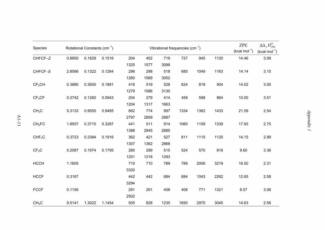
Appendix 1
A1-11
Species Rotational Constants (cm−1) Vibrational frequencies (cm−1)ZPE
(kcal mol−1)
∆∆ f H2980
(kcal mol−1)
CHFCF−Z 0.8850 0.1829 0.1516 204 402 719 727 945 1120 14.46 3.09
1325 1577 3099
CHFCF−E 2.8566 0.1322 0.1264 296 298 518 685 1049 1163 14.14 3.15
1260 1569 3052
CF2CH 0.3880 0.3650 0.1881 416 519 528 624 819 904 14.02 3.00
1279 1586 3130
CF2CF 0.3742 0.1260 0.0943 204 279 414 459 588 864 10.00 3.51
1204 1317 1663
CH3C 5.3133 0.9550 0.9485 662 774 997 1334 1362 1433 21.59 2.54
2797 2859 2887
CH2FC 1.8557 0.3715 0.3287 441 511 914 1060 1159 1339 17.93 2.75
1388 2845 2885
CHF2C 0.3723 0.3384 0.1916 362 421 527 811 1115 1125 14.15 2.99
1307 1362 2868
CF3C 0.2087 0.1974 0.1795 280 299 515 524 570 816 9.60 3.36
1201 1218 1293
HCCH 1.1605 710 710 789 789 2006 3219 16.50 2.31
3320
HCCF 0.3167 442 442 684 684 1043 2262 12.65 2.58
3294
FCCF 0.1156 291 291 408 408 771 1321 8.57 3.06
2502
CH2C 9.5141 1.3022 1.1454 505 828 1235 1650 2970 3045 14.63 2.56

Appendix 1
A1-12
Species Rotational Constants (cm−1) Vibrational frequencies (cm−1)ZPE
(kcal mol−1)
∆∆ f H2980
(kcal mol−1)
CHFC 3.4765 0.3821 0.3443 360 780 1044 1157 1691 3018 11.51 2.68
CF2C 0.4245 0.3592 0.1946 351 494 585 928 1297 1706 7.67 2.88
CCH 1.5328 496 496 1654 3234 8.41 2.36
CCF 0.3697 218 218 1003 2072 5.02 2.77
CH2CO 9.4884 0.3370 0.3254 439 555 646 993 1131 1399 19.17 2.79
2124 3015 3105
CHFCO 1.7613 0.1517 0.1396 242 472 561 668 1024 1169 15.44 3.07
1408 2152 3106
CF2CO 0.3491 0.1288 0.0941 207 273 378 442 673 794 11.07 3.52
1315 1451 2209
CHCO 27.3099 0.3613 0.3565 485 553 606 1172 2207 3013 11.49 2.75
CFCO 37.0140 0.1318 0.1314 204 433 590 940 1691 2286 8.78 3.03
CH3CHO 1.8856 0.3366 0.3016 136 488 764 861 1099 1129 33.58 3.08
1371 1398 1434 1443 1815 2812
2863 2912 2964
CH2FCHO 1.3230 0.1429 0.1322 85 315 515 721 1019 1078 29.72 3.38
1105 1222 1328 1392 1461 1821
2858 2911 2960
CHF2CHO 0.3075 0.1291 0.0998 76 316 369 416 592 978 25.57 3.70
1082 1128 1131 1312 1369 1395
1841 2875 3003
CF3CHO 0.1806 0.0993 0.0977 71 251 309 423 515 515 20.73 4.05
688 835 981 1225 1225 1330
1383 1858 2894

Appendix 1
A1-13
Species Rotational Constants (cm−1) Vibrational frequencies (cm−1)ZPE
(kcal mol−1)
∆∆ f H2980
(kcal mol−1)
CH3CFO 0.3606 0.3236 0.1761 130 394 561 585 837 1002 29.72 3.32
1059 1222 1398 1438 1444 1894
2887 2945 2991
CH2FCFO 0.3440 0.1286 0.0953 112 243 443 528 635 870 25.84 3.62
1034 1121 1167 1238 1421 1468
1925 2913 2960
CHF2CFO 0.1786 0.1107 0.0745 53 224 311 427 542 586 21.50 4.02
747 924 1116 1183 1211 1381
1424 1932 2975
CF3CFO 0.1256 0.0834 0.0686 47 219 233 375 417 501 16.57 4.41
578 678 763 801 1122 1244
1293 1373 1944
CH3CO 2.7440 0.3313 0.3128 87 454 826 938 1037 1356 26.08 3.12
1432 1433 1911 2871 2946 2950
CH2FCO 1.6312 0.1424 0.1343 137 312 496 842 895 1100 22.29 3.30
1215 1346 1451 1925 2908 2964
CHF2CO 0.3213 0.1323 0.1002 57 367 407 411 590 947 18.11 3.65
1133 1150 1319 1366 1940 2977
CF3CO 0.1856 0.1000 0.1000 57 234 388 412 523 531 13.27 4.01
667 795 1203 1241 1268 1960
a ∆∆ ∆ ∆f f fH H H2980
2980
00= −
b Computed from HF/6-31G(d) geometry.

Appendix 1
A1-14
Appendix 1.4 C3 Hydrofluorocarbons: Rotational constants and vibrational frequencies (scaled by 0.8929) obtained at MP2(Full)/6-31G(d)
and HF/6-31G(d) levels of theory respectively and the resulting zero point energies and thermal correctionsa to the heats of formation.
Species Rotational Constants (cm−1) Vibrational frequencies (cm−1)ZPE
(kcal mol−1)
∆∆ f H2980
(kcal mol−1)
C3H6 1.5495 0.3109 0.2720 189 407 572 880 919 954 47.88 3.21
1008 1060 1158 1289 1389 1424
1451 1464 1679 2852 2895 2923
2964 2976 3039
C3H7 1.0384 0.2983 0.2674 118 241 314 481 713 855 52.93 3.76
860 997 1049 1171 1277 1315
1388 1432 1458 1466 1475 2853
2858 2881 2912 2917 2952 3039
C3F6 0.0840 0.0419 0.0328 36 125 170 238 245 351 21.39 5.61
358 457 497 566 586 638
660 751 1025 1198 1228 1254
1342 1404 1832
C3F6H 0.0760 0.0460 0.0398 34 89 143 204 234 287 28.08 5.82
348 447 509 517 567 623
740 840 924 1123 1176 1239
1247 1296 1314 1379 1403 2963
a ∆∆ ∆ ∆f f fH H H2980
2980
00= −

Appendix 2
A2-1
Appendix 2: Phosphorus Compounds
Supplementary Information
Appendix 2.1 Geometric data for molecules in Table 4.1. Bond lengths in Å, angles in
degrees, rotational constants and vibrational frequencies in cm−1.
H2 - 1ΣΣΣΣg - D∞h
G3
Z-matrix
H(1)H(2) 1 0.7375
Rotational Constant
61.5135
Vibrational Frequency
4149
G3X
Z-matrix
H(1)H(2) 1 0.7427
Rotational Constant
60.6414
Vibrational Frequency
4401
H(2)H(1)

Appendix 2
A2-2
O2 - 3ΣΣΣΣg - D∞h
G3
Z-matrix
O(1)O(2) 1 1.2460
Rotational Constant
1.3578
Vibrational Frequency
1784
G3X
Z-matrix
O(1)O(2) 1 1.2064
Rotational Constant
1.4484
Vibrational Frequency
1640
O(2)O(1)

Appendix 2
A2-3
P2 - 1ΣΣΣΣg - D∞h
G3
Z-matrix
P(1)P(2) 1 1.9324
Rotational Constant0.2915
Vibrational Frequency
811
G3X
Z-matrix
P(1)P(2) 1 1.8952
Rotational Constant0.3031
Vibrational Frequency
793
P(2)P(1)

Appendix 2
A2-4
P4 - 1A1 - Td
G3
Z-matrix
P(1)P(2) 1 2.1948P(3) 1 2.1948 2 60.0P(4) 1 2.1948 2 60.0 3 -70.5
Rotational Constants
0.1130, 0.1130, 0.1130
Vibrational Frequencies
363, 363, 466, 466, 466, 615
G3X
Z-matrix
P(1)P(2) 1 2.2112P(3) 1 2.2112 2 60.0P(4) 1 2.2112 2 60.0 3 -70.5
Rotational Constants
0.1113, 0.1113, 0.1113
Vibrational Frequencies
363, 363, 454, 454, 454, 599
P(3) P(4)
P(1)
P(2)

Appendix 2
A2-5
HO - 2ΠΠΠΠ - C∞v
G3
Z-matrix
O(1)H(2) 1 0.9790
Rotational Constant
18.5531
Vibrational Frequency
3569
G3X
Z-matrix
O(1)H(2) 1 0.9761
Rotational Constant
18.6606
Vibrational Frequency
3642
H(2)O(1)

Appendix 2
A2-6
H2O - 1A1 - C2v
G3
Z-matrix
O(1)H(2) 1 0.9686H(3) 1 0.9686 2 103.9
Rotational Constants
26.4131, 14.3801, 9.3109
Vibrational Frequencies
1631, 3635, 3740
G3X
Z-matrix
O(1)H(2) 1 0.9620H(3) 1 0.9620 2 103.7
Rotational Constants
26.6798, 14.6088, 9.4399
Vibrational Frequencies
1647, 3749, 3852
H(2)
O(1)
H(3)
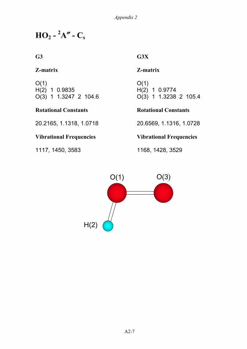
Appendix 2
A2-7
HO2 - 2A″″″″ - Cs
G3
Z-matrix
O(1)H(2) 1 0.9835O(3) 1 1.3247 2 104.6
Rotational Constants
20.2165, 1.1318, 1.0718
Vibrational Frequencies
1117, 1450, 3583
G3X
Z-matrix
O(1)H(2) 1 0.9774O(3) 1 1.3238 2 105.4
Rotational Constants
20.6569, 1.1316, 1.0728
Vibrational Frequencies
1168, 1428, 3529
H(2)
O(1) O(3)
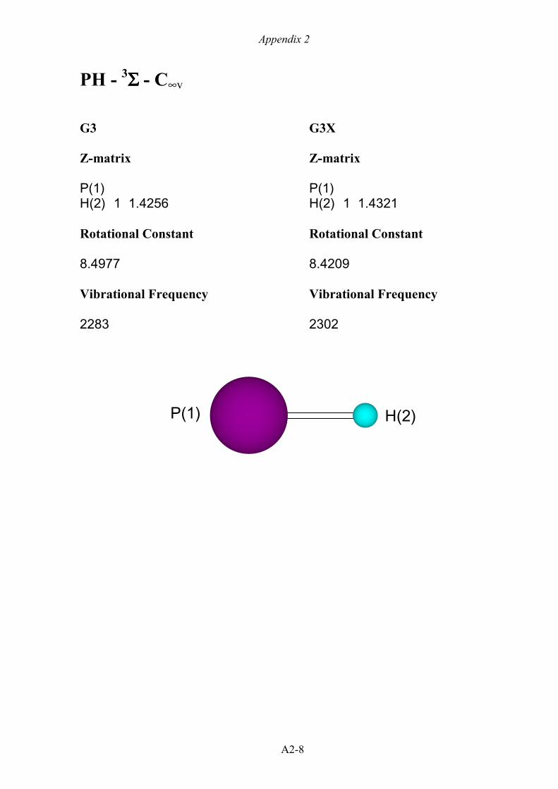
Appendix 2
A2-8
PH - 3ΣΣΣΣ - C∞v
G3
Z-matrix
P(1)H(2) 1 1.4256
Rotational Constant
8.4977
Vibrational Frequency
2283
G3X
Z-matrix
P(1)H(2) 1 1.4321
Rotational Constant
8.4209
Vibrational Frequency
2302
H(2)P(1)

Appendix 2
A2-9
PH2 - 2B1 - C2v
G3
Z-matrix
P(1)H(2) 1 1.4199H(3) 1 1.4199 2 92.5
Rotational Constants
9.2479, 7.9442, 4.2733
Vibrational Frequencies
1123, 2302, 2303
G3X
Z-matrix
P(1)H(2) 1 1.4265H(3) 1 1.4265 2 91.6
Rotational Constants
9.0041, 7.9990, 4.2359
Vibrational Frequencies
1113, 2328, 2338
H(2)
P(1)
H(3)

Appendix 2
A2-10
PH3 - 1A′′′′ - Cs
G3
Z-matrix
P(1)H(2) 1 1.4146H(3) 1 1.4146 2 94.6H(4) 1 1.4146 2 94.6 3 95.0
Rotational Constants
4.5307, 4.5304, 3.8680
Vibrational Frequencies
1018, 1135, 1135, 2323, 2325,2330
G3X
Z-matrix
P(1)H(2) 1 1.4219H(3) 1 1.4219 2 93.3H(4) 1 1.4219 2 93.3 3 93.5
Rotational Constants
4.4376, 4.4374, 3.9147
Vibrational Frequencies
1010, 1126, 1126, 2355, 2364,2367
H(4)H(2)
P(1)
H(3)

Appendix 2
A2-11
P2H2 - 1Ag - Cs
G3
Z-matrix
P(1)P(2) 1 2.0429H(3) 1 1.4221 2 94.7H(4) 2 1.4221 1 94.7 3 180.0
Rotational Constants
4.3429, 0.2501, 0.2364
Vibrational Frequencies
626, 686, 775, 961, 2299, 2311
G3X
Z-matrix
P(1)P(2) 1 2.0351H(3) 1 1.4294 2 94.2H(4) 2 1.4294 1 94.2 3 180.0
Rotational Constants
4.2893, 0.2522, 0.2382
Vibrational Frequencies
611, 678, 766, 962, 2298, 2313
H(4)
P(1)
P(2)
H(3)

Appendix 2
A2-12
P2H4 - 1Ag - Cs
G3
Z-matrix
P(1)P(2) 1 2.2311H(3) 1 1.4170 2 95.2H(4) 1 1.4170 2 95.2 3 -94.1H(5) 2 1.4170 1 95.2 3 -85.9H(6) 2 1.4170 1 95.2 3 180.0
Rotational Constants
2.1786, 0.1937, 0.1917
Vibrational Frequencies
58, 436, 622, 649, 869, 908,1103, 1106, 2311, 2319, 2321,2324
G3X
Z-matrix
P(1)P(2) 1 2.2594H(3) 1 1.4242 2 93.8H(4) 1 1.4242 1 93.8 3 -92.4H(4) 2 1.4242 1 93.8 3 -87.6H(4) 2 1.4242 1 93.8 3 180.0
Rotational Constants
2.1468, 0.1894, 0.1881
Vibrational Frequencies
103, 422, 613, 629, 854, 896,1084, 1093, 2333, 2338, 2340,2351
H(4)
H(5)
P(1)
P(2)
H(3)
H(6)

Appendix 2
A2-13
PO - 2ΠΠΠΠ - C∞v
G3
Z-matrix
P(1)O(2) 1 1.4715
Rotational Constant
0.7381
Vibrational Frequency
1254
G3X
Z-matrix
P(1)O(2) 1 1.4831
Rotational Constant
0.7266
Vibrational Frequency
1241
O(2)P(1)

Appendix 2
A2-14
PO2 - 2A1 - C2v
G3
Z-matrix
P(1)O(2) 1 1.4924O(3) 1 1.4924 2 136.4
Rotational Constants
3.4850, 0.2745, 0.2544
Vibrational Frequencies
409, 1079, 1301
G3X
Z-matrix
P(1)O(2) 1 1.4743O(3) 1 1.4743 2 134.4
Rotational Constants
3.2851, 0.2852, 0.2625
Vibrational Frequencies
378, 1061, 1314
O(2)
P(1)
O(3)

Appendix 2
A2-15
PO3 - 2A2′′′′ - D3h
G3
Z-matrix
P(1)O(2) 1 1.5025O(3) 1 1.5025 2 120.0O(4) 1 1.5025 2 120.0 3 180.0
Rotational Constants
0.3112, 0.3112, 0.1556
Vibrational Frequencies
442, 442, 443, 1028, 1690, 1690
G3X
Z-matrix
P(1)O(2) 1 1.4792O(3) 1 1.4792 2 120.0O(4) 1 1.4792 2 120.0 3 180.0
Rotational Constants
0.3211, 0.3211, 0.1606
Vibrational Frequencies
152, 152, 424, 1009, 1107, 1108
O(4)
P(1)
O(2)
O(3)

Appendix 2
A2-16
PO3 - 2B2 - C2v
Z-matrix
P(1)O(2) 1 1.6076O(3) 1 1.4726 2 111.4O(4) 1 1.4726 2 111.4 3 180.0
Rotational Constants
0.3394, 0.2804, 0.1535
Vibrational Frequencies
343, 431, 434, 856, 1176, 1465
O(3)
P(1)
O(2)
O(4)

Appendix 2
A2-17
PPO - 1ΣΣΣΣ - C∞v
G3
Z-matrix
P(1)P(2) 1 1.9217O(3) 1 1.5029 2 180.0
Rotational Constant
0.1255
Vibrational Frequencies
179, 179, 669, 1275
G3X
Z-matrix
P(1)P(2) 1 1.8926O(3) 1 1.4730 2 180.0
Rotational Constant
0.1298
Vibrational Frequencies
214, 215, 657, 1294
P(2) P(1)O(3)

Appendix 2
A2-18
P2O - 1A1 - C2v
Z-matrix
P(1)O(2) 1 1.7755P(3) 2 1.7755 1 69.0
Rotational Constants
0.6193, 0.2691, 0.1876
Vibrational Frequencies
241, 655, 825
O(2)
P(3)P(1)

Appendix 2
A2-19
P2O2 - 1Ag - D2h
G3
Z-matrix
P(1)O(2) 1 1.6916P(3) 2 1.6916 1 96.6O(4) 3 1.6916 2 83.4 1 0.0
Rotational Constants
0.4158, 0.1707, 0.1210
Vibrational Frequencies
24, 446, 615, 720, 759, 912
G3X
Z-matrix
P(1)O(2) 1 1.6611P(3) 2 1.6611 1 96.5O(4) 3 1.6620 2 83.6 1 0.0
Rotational Constants
0.4298, 0.1773, 0.1255
Vibrational Frequencies
445, 552, 619, 708, 731, 876
O(2)
P(3)P(1)
O(4)

Appendix 2
A2-20
P2O2 - C1
Z-matrix
P(1)O(2) 1 1.7500P(3) 2 1.7479 1 70.9O(4) 3 1.7491 2 83.9 1 50.2
Rotational Constants
0.2922, 0.2168, 0.1569
Vibrational Frequencies
385, 396, 513, 652, 785, 877
O(4)
P(1) P(3)
O(2)

Appendix 2
A2-21
P2O2 - 3A″″″″ - Cs
Z-matrix
P(1)O(2) 1 1.6977P(3) 2 1.6559 1 129.6O(4) 3 1.4938 2 111.5 1 0.0
Rotational Constants
0.4799, 0.0959, 0.0799
Vibrational Frequencies
129, 168, 463, 591, 875, 1275
P(1)
O(2)
P(3)
O(4)

Appendix 2
A2-22
P2O2 - 3A″″″″ - Cs
Z-matrix
P(1)O(2) 1 1.6836P(3) 2 1.6645 1 128.0O(4) 3 1.4895 2 108.6 1 180.0
Rotational Constants
1.2663, 0.0729, 0.0690
Vibrational Frequencies
93, 137, 346, 646, 893, 1291
P(1)
O(2)
P(3)
O(4)

Appendix 2
A2-23
P2O3 - 1A - C2
G3
Z-matrix
O(1)P(2) 1 1.4920O(3) 2 1.6787 1 111.1P(4) 3 1.6787 2 135.3 1 28.3O(5) 4 1.4920 3 111.1 2 28.3
Rotational Constants
0.2676, 0.0693, 0.0584
Vibrational Frequencies
76, 86, 98, 389, 497, 571,833, 1279, 1296
G3X
Z-matrix
O(1)P(2) 1 1.4665O(3) 2 1.6499 1 110.6P(4) 3 1.6499 2 143.8 1 34.5O(5) 4 1.4665 3 110.6 2 34.5
Rotational Constants
0.3024, 0.0636, 0.0567
Vibrational Frequencies
52, 72, 94, 390, 459, 555,841, 1267, 1282
O(1)
P(4)
O(3)
P(2)
O(5)

Appendix 2
A2-24
HPO - 1A′′′′ - Cs
G3
Z-matrix
P(1)O(2) 1 1.5170H(3) 1 1.4530 2 105.6
Rotational Constants
9.0393, 0.6702, 0.6239
Vibrational Frequencies
1007, 1228, 2153
G3X
Z-matrix
P(1)O(2) 1 1.4851H(3) 1 1.4727 2 104.9
Rotational Constants
8.7388, 0.6994, 0.6475
Vibrational Frequencies
998, 1212, 2052
O(2)
P(1)
H(3)
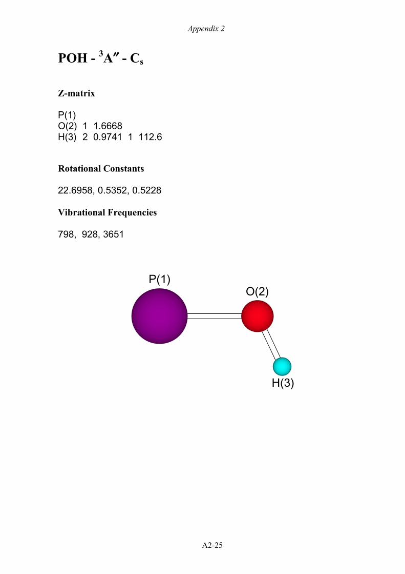
Appendix 2
A2-25
POH - 3A″″″″ - Cs
Z-matrix
P(1)O(2) 1 1.6668H(3) 2 0.9741 1 112.6
Rotational Constants
22.6958, 0.5352, 0.5228
Vibrational Frequencies
798, 928, 3651
O(2)P(1)
H(3)

Appendix 2
A2-26
HPOH - 2A″″″″ - Cs
G3
Z-matrix
P(1)O(2) 1 1.6759H(3) 1 1.4161 2 93.8H(4) 2 0.9730 1 108.9 3 180.0
Rotational Constants
6.2768, 0.5224, 0.4823
Vibrational Frequencies
364, 795, 891, 1091, 2322, 3669
G3X
Z-matrix
P(1)O(2) 1 1.6585H(3) 1 1.4276 2 93.9H(4) 2 0.9637 1 109.7 3 180.0
Rotational Constants
6.2639, 0.5326, 0.4909
Vibrational Frequencies
441, 812, 913, 1115, 2312, 3772
H(3)
P(1)
O(2)
H(4)

Appendix 2
A2-27
HPOH - 2A″″″″ - Cs
Z-matrix
P(1)O(2) 1 1.6701H(3) 1 1.4284 2 98.8H(4) 2 0.9714 1 113.7 3 0.0
Rotational Constants
6.2564, 0.5222, 0.4820
Vibrational Frequencies
178, 797, 878, 1069, 2248, 3685
H(3)
P(1)O(2)
H(4)

Appendix 2
A2-28
H3PO - 1A1 - C3v
G3
Z-matrix
P(1)O(2) 1 1.4977H(3) 1 1.4112 2 117.5H(4) 1 1.4112 2 117.5 3 120.0H(5) 1 1.4112 2 117.5 3 -120.0
Rotational Constants
3.5612, 0.5645, 0.565
Vibrational Frequencies
855, 855, 1112, 1112, 1147, 1247,2380, 2380, 2405
G3X
Z-matrix
P(1)O(2) 1 1.4787H(3) 1 1.4187 2 117.3H(4) 1 1.4187 2 117.3 3 120.0H(5) 1 1.4187 2 117.3 3 -120.0
Rotational Constants
3.5060, 0.5764, 0.5764
Vibrational Frequencies
834, 834, 1104, 1104, 1143,1264, 2345, 2345, 2366
H(4) H(5)
P(1)
O(2)
H(3)

Appendix 2
A2-29
H2POH - 1A′′′′ - Cs
G3
Z-matrix
P(1)O(2) 1 1.6803H(3) 2 0.9705 1 108.0H(4) 1 1.4159 2 99.1 3 132.5H(5) 1 1.4159 2 99.1 3 -132.5
Rotational Constants
3.7301, 0.4754, 0.4722
Vibrational Frequencies
262, 785, 895, 899, 1117, 1142,2321, 2331, 3688
G3X
Z-matrix
P(1)O(2) 1 1.6634H(3) 2 0.9610 1 108.6H(4) 1 1.4267 2 98.8 3 133.4H(5) 1 1.4267 2 98.8 3 -133.4
Rotational Constants
3.6995, 0.4845, 0.4801
Vibrational Frequencies
257, 788, 912, 925, 1137, 1144,2313, 2313, 3804
H(4)
P(1)
O(2)
H(3)
H(5)
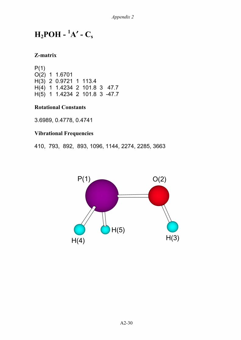
Appendix 2
A2-30
H2POH - 1A′′′′ - Cs
Z-matrix
P(1)O(2) 1 1.6701H(3) 2 0.9721 1 113.4H(4) 1 1.4234 2 101.8 3 47.7H(5) 1 1.4234 2 101.8 3 -47.7
Rotational Constants
3.6989, 0.4778, 0.4741
Vibrational Frequencies
410, 793, 892, 893, 1096, 1144, 2274, 2285, 3663
H(5)
P(1) O(2)
H(3)H(4)

Appendix 2
A2-31
HOPO - 1A′′′′ - Cs
G3
Z-matrix
P(1)O(2) 1 1.6380O(3) 1 1.4960 2 110.5H(4) 2 0.9816 1 112.1 3 0.0
Rotational Constants
1.1834, 0.3082, 0.2445
Vibrational Frequencies
394, 546, 848, 956, 1274, 3591
G3X
Z-matrix
P(1)O(2) 1 1.6163O(3) 1 1.4726 2 111.0H(4) 2 0.9706 1 113.6 3 0.0
Rotational Constants
1.2306, 0.3150, 0.2508
Vibrational Frequencies
379, 556, 837, 944, 1263, 3681
O(3)
P(1)O(2)
H(4)

Appendix 2
A2-32
HOPO - 1A′′′′ - Cs
Z-matrix
P(1)O(2) 1 1.6432O(3) 1 1.4900 2 108.8H(4) 2 0.9771 1 110.6 3 180.0
Rotational Constants
1.2970, 0.2980, 0.2423
Vibrational Frequencies
408, 450, 828, 952, 1296, 3637
O(3)
P(1)
O(2)
H(4)

Appendix 2
A2-33
HPO2 - 1A1 - C2v
Z-matrix
P(1)O(2) 1 1.4793O(3) 1 1.4793 2 134.9H(4) 1 1.4034 2 112.5 3 180.0
Rotational Constants
2.1344, 0.2823, 0.2493
Vibrational Frequencies
475, 663, 1053, 1151, 1454, 2476
O(2)
P(1)
H(4)
O(3)

Appendix 2
A2-34
HOPO2 - 1A′′′′ - Cs
G3
Z-matrix
P(1)O(2) 1 1.6047O(3) 1 1.4728 2 112.1O(4) 1 1.4788 2 113.5 3 180.0H(5) 2 0.9779 1 110.5 3 180.0
Rotational Constants
0.3110, 0.2799, 0.1473
Vibrational Frequencies
391, 433, 450, 515, 899, 1028,1180, 1445, 3623
G3X
Z-matrix
P(1)O(2) 1 1.5846O(3) 1 1.4536 2 112.0O(4) 1 1.4591 2 113.9 3 180.0H(5) 2 0.9677 1 111.2 3 180.0
Rotational Constants
0.3175, 0.2883, 0.1511
Vibrational Frequencies
391, 424, 435, 502, 889, 1036,1179, 1452, 3736
O(3)
P(1)
O(4)
O(2)
H(5)

Appendix 2
A2-35
Appendix 2.2 Computed Heats of Reaction for Twarowski’sa data set.
Reaction No. Reaction0298r H∆ (kcal mol−1)
G3 G3Xb Literaturec Diff(G3X−Lit)
1 H + H → H2 −104.7 −104.6 −104.2 −0.4
2 O + O → O2 −118.0 −119.1 −119.1 0.0
3 H + O → OH −103.2 −103.2 −102.8 −0.4
4 H + OH → H2O −118.0 −118.0 −118.7 0.7
5 H + O2 → HO2 −49.9 −48.9 −48.8 −0.1
6 H + O2 → OH + O 14.8 15.9 16.3 −0.4
7 H2 + OH → H2O + H −13.3 −13.4 −14.5 1.1
8 OH + OH → O + H2O −14.7 −14.8 −15.9 1.1
9 O + H2 → OH + H 1.4 1.4 1.4 0.0
10 HO2 + H → OH + OH −38.6 −38.4 −37.7 −0.7
11 HO2 + H → H2 + O2 −54.8 −55.7 −55.4 −0.3
12 HO2 + O → O2 + OH −53.3 −54.3 −54.0 −0.3
13 HO2 + OH → H2O + O2 −68.1 −69.1 −69.9 0.8
14 H + PO → HPO −65.1 −65.4 −66.9 1.5
15 H + PO2 → HOPO −92.9 −92.2 −94.2 2.0
16 H + PO3 → HOPO2 −115.2 −113.2 −116.0 2.8
17 H + HPO → HPOH −54.1 −53.5
18 H + P → PH −71.7 −72.0
19 PH2 + H → PH3 −81.6 −81.8
20 PH + H → PH2 −75.5 −75.6
21 HPOH + H → H2POH −76.5 −77.3
22 O + PO → PO2 −119.5 −120.9 −122.0 1.1
23 PO2 + O → PO3 −93.7 −95.8 −96.8 1.0
24 HOPO + O → HOPO2 −116.0 −116.7 −118.6 1.9
25 P + O → PO −142.7 −143.9 −143.0 −0.9
26 P2 + O → P2O −89.5 −72.5
27 PH + O → HPO −136.1 −137.3
28 O + P2O → P2O2 −124.8 −126.2
29 OH + PO → HOPO −109.1 −110.0 −113.4 3.5
30 OH + PO2 → HOPO2 −105.7 −105.7 −109.9 4.2
31 OH + PH2 → H2POH −87.9 −89.2
32 PH + OH → HPOH −86.9 −87.5
33 PO + PO → P2O2 −44.6 −46.0
34 PO + PO2 → P2O3 −76.0 −76.4
35 PO + P → P2O −62.5 −63.6
36 P + P → P2 −115.8 −135.0

Appendix 2
A2-36
Reaction No. Reaction0298r H∆ (kcal mol−1)
G3 G3Xb Literaturec Diff(G3X−Lit)
37 P2 + P2 → P4 −52.7 −52.3
38 H2O + PO3 → OH + HOPO2 2.8 4.9 2.7 2.1
39 H2 + PO3 → HOPO2 + H −10.5 −8.6 −11.8 3.2
40 O2 + PO → O + PO2 −1.5 −1.8 −2.9 1.1
41 P + O2 → O + PO −24.8 −24.8 −23.9 −0.9
42 O2 + PH → O + HPO −18.1 −18.2
43 H + HOPO → H2O + PO −8.8 −8.0 −5.3 −2.7
44 H + HOPO → H2 + PO2 −11.8 −12.4 −10.0 −2.4
45 H + HOPO2 → H2O + PO2 −12.3 −12.3 −8.8 −3.5
46 H + PO3 → O + HOPO 0.9 3.5 2.5 1.0
47 H + PO3 → OH + PO2 −9.5 −7.4 −6.1 −1.4
48 H + P2O3 → HOPO + PO −16.9 −15.8
49 H + HPO → H2 + PO −39.6 −39.2 −37.3 −1.9
50 H + PH3 → H2 + PH2 −23.0 −22.8
51 H + PH2 → H2 + PH −29.2 −29.0
52 H + PH → H2 + P −32.9 −32.6
53 H + P2O → OH + P2 −13.7 −30.7
54 H + P2O → PO + PH −9.2 −8.4
55 H + P2O → HPO + P −2.5 −1.8
56 H + P2O2 → PO + HPO −20.4 −19.5
57 H + H2POH → H2O + PH2 −30.0 −28.8
58 H + H2POH → H2 + HPOH −28.2 −27.3
59 H + HPOH → H2O + PH −31.0 −30.5
60 H + HPOH → H2 + HPO −50.6 −51.1
61 O + HOPO → OH + PO2 −10.4 −11.0 −8.6 −2.4
62 O + HOPO2 → O2 + HOPO −1.9 −2.4 −0.6 −1.8
63 O + PO3 → O2 + PO2 −24.3 −23.3 −22.3 −1.0
64 O + P2O3 → PO + PO3 −17.7 −19.4
65 O + P2O3 → PO2 + PO2 −43.6 −44.5
66 O + HPO → H + PO2 −54.5 −55.5 −55.1 −0.4
67 O + HPO → OH + PO −38.2 −37.8 −35.9 −1.9
68 O + P2 → P + PO −27.0 −8.9
69 O + PH3 → OH + PH2 −21.6 −21.4
70 O + PH2 → H + HPO −60.6 −61.6
71 O + PH2 → OH + PH −27.8 −27.6
72 O + PH → H + PO −71.0 −71.9
73 O + PH → OH + P −31.5 −31.2

Appendix 2
A2-37
Reaction No. Reaction0298r H∆ (kcal mol−1)
G3 G3Xb Literaturec Diff(G3X−Lit)
74 O + P2O → O2 + P2 −28.5 −46.6
75 O + P2O → PO + PO −80.2 −80.3
76 O + P2O → PO2 + P −57.0 −57.3
77 O + P2O2 → O2 + P2O 6.8 7.1
78 O + P2O2 → PO + PO2 −74.9 −75.0
79 O + H2POH → OH + HPOH −26.8 −25.9
80 O + HPOH → H + HOPO −93.2 −94.3
81 O + HPOH → OH + HPO −49.1 −49.7
82 OH + PO → H + PO2 −16.3 −17.7 −19.2 1.5
83 OH + HOPO → H2O + PO2 −25.1 −25.8 −24.5 −1.3
84 OH + HOPO → H + HOPO2 −12.8 −13.5 −15.7 2.2
85 OH + PO3 → O + HOPO2 −12.0 −10.0 −13.2 3.2
86 OH + P2O3 → PO + HOPO2 −29.7 −29.3
87 OH + P2O3 → PO2 + HOPO −33.2 −33.6
88 OH + HPO → H2O + PO −52.9 −52.6 −51.8 −0.8
89 OH + HPO → H + HOPO −44.1 −44.6 −46.5 2.0
90 OH + P → H + PO −39.5 −40.7 −40.1 −0.5
91 OH + PH3 → H2O + PH2 −36.4 −36.2
92 OH + PH3 → H + H2POH −6.3 −7.3
93 OH + PH2 → H2O + PH −42.5 −42.4
94 OH + PH2 → H + HPOH −11.5 −11.9
95 OH + PH → H2O + P −46.3 −46.0
96 OH + PH → H + HPO −32.8 −34.1
97 OH + P2O → H + P2O2 −21.6 −23.0
98 OH + P2O → P + HOPO −46.6 −46.4
99 OH + P2O2 → PO + HOPO −64.5 −64.0
100 OH + H2POH → H2O + HPOH −41.5 −40.7
101 OH + HPOH → H2O + HPO −63.9 −64.6
102 HO2 + PO → O2 + HPO −15.1 −16.5 −18.1 1.6
103 HO2 + PO → O + HOPO −44.5 −45.2 −48.4 3.2
104 HO2 + PO → OH + PO2 −54.9 −56.2 −57.0 0.8
105 HO2 + PO2 → O2 + HOPO −42.9 −43.4 −45.4 2.1
106 HO2 + PO2 → O + HOPO2 −41.0 −41.0 −44.9 3.9
107 HO2 + PO2 → OH + PO3 −29.1 −31.0 −31.7 0.7
108 HO2 + HOPO → OH + HOPO2 −51.4 −51.9 −53.5 1.6
109 HO2 + PO3 → O2 + HOPO2 −65.3 −64.3 −67.2 2.9
110 HO2 + HPO → O2 + HPOH −4.2 −4.6

Appendix 2
A2-38
Reaction No. Reaction0298r H∆ (kcal mol−1)
G3 G3Xb Literaturec Diff(G3X−Lit)
111 HO2 + P → O2 + PH −21.8 −23.1
112 HO2 + P → OH + PO −78.1 −79.1 −77.9 −1.2
113 HO2 + P2 → OH + P2O −24.9 −7.7
114 HO2 + PH2 → O2 + PH3 −31.7 −32.9
115 HO2 + PH2 → O + H2POH −23.3 −24.4
116 HO2 + PH → O2 + PH2 −25.6 −26.8
117 HO2 + PH → O + HPOH −22.3 −22.8
118 HO2 + PH → OH + HPO −71.4 −72.5
119 HO2 + P2O → OH + P2O2 −60.2 −61.4
120 HO2 + HPOH → O2 + H2POH −26.6 −28.4
121 PO + HOPO2 → HOPO + PO2 −3.5 −4.2 −3.5 −0.7
122 PO + PO3 → PO2 + PO2 −25.8 −25.2 −25.3 0.1
123 PO + P2O → PO2 + P2 −30.0 −48.4
124 PO + P2O2 → PO2 + P2O 5.3 5.3
125 PO + H2POH → HOPO + PH2 −21.2 −20.8
126 PO + HPOH → HOPO + PH −22.2 −22.4
127 PO + HPOH → HPO + HPO −11.0 −11.9
128 PO2 + HPO → H + P2O3 −10.9 −11.0
129 PO2 + HPO → PO + HOPO −27.8 −26.8 −27.3 0.5
130 PO2 + P → PO + PO −23.2 −23.0 −20.9 −2.0
131 PO2 + PH3 → HOPO + PH2 −11.2 −10.4
132 PO2 + PH2 → HOPO + PH −17.4 −16.6
133 PO2 + PH → PO + HPO −16.6 −16.3
134 PO2 + PH → HOPO + P −21.1 −20.2
136 PO2 + P2O → PO3 + P2 −4.2 −23.3
136 PO2 + P2O → P2O3 + P −13.4 −12.8
137 PO2 + P2O → PO + P2O3 −31.4 −30.5
138 PO2 + H2POH → HOPO + HPOH −16.4 −15.0
139 PO2 + H2POH → HOPO2 + PH2 −17.7 −16.6
140 PO2 + HPOH → HOPO + HPO −38.8 −38.8
141 PO2 + HPOH → HOPO2 + PH −18.7 −18.2
142 HOPO + PO3 → PO2 + HOPO2 −22.3 −20.9 −21.8 0.9
143 HOPO + P2O → HOPO2 + P2 −26.5 −44.2
145 HOPO + P2O2 → HOPO2 + P2O 8.8 9.5
145 HOPO2 + P → PO + HOPO −26.7 −27.2 −24.4 −2.8
146 HOPO2 + PH → HOPO + HPO −20.0 −20.6
147 PO3 + HPO → PO + HOPO2 −50.1 −47.8 −49.1 1.3

Appendix 2
A2-39
Reaction No. Reaction0298r H∆ (kcal mol−1)
G3 G3Xb Literaturec Diff(G3X−Lit)
148 PO3 + P → PO + PO2 −49.0 −48.1 −46.2 −1.9
149 PO3 + PH3 → HOPO2 + PH2 −33.6 −31.3
150 PO3 + PH2 → HOPO2 + PH −39.7 −37.5
152 PO3 + PH → HPO + PO2 −42.4 −41.5
152 PO3 + PH → HOPO2 + P −43.5 −41.1
153 PO3 + P2O → PO2 + P2O2 −31.1 −30.4
154 PO3 + H2POH → HOPO2 + HPOH −38.7 −35.9
156 PO3 + HPOH → HOPO2 + HPO −61.1 −59.7
156 HPO + P → PO + PH −6.7 −6.6
157 HPO + PH2 → PO + PH3 −16.6 −16.4
158 HPO + PH → PO + PH2 −10.4 −10.2
159 HPO + HPOH → PO + H2POH −11.4 −11.9
161 P + PH → H + P2 −44.0 −63.0
161 P + P2O → PO + P2 −53.2 −71.4
162 P + P2O2 → PO + P2O −17.9 −17.7
164 P + HPOH → HPO + PH −17.6 −18.6
164 PH + PH3 → PH2 + PH2 6.1 6.2
165 PH3 + HPOH → PH2 + H2POH 5.1 4.6
166 PH2 + PH → P + PH3 −9.9 −9.8
168 PH2 + HPOH → HPO + PH3 −27.5 −28.4
168 PH + PH → P + PH2 −3.7 −3.6
169 PH + P2O → HPO + P2 −46.5 −64.8
170 PH + P2O2 → HPO + P2O −11.3 −11.1
171 PH + H2POH → PH2 + HPOH 1.0 1.6
172 PH + HPOH → HPO + PH2 −21.4 −22.2
173 PH + HPOH → P + H2POH −4.7 −5.3
174 P2O + P2O → P2 + P2O2 −35.3 −53.7
175 HPOH + HPOH → HPO + H2POH −22.4 −23.8
a A. Twarowski, Combustion and Flame, 1995, 102, 41.
b Using experimental 0298f H∆ for H, O and P and G3X(RAD) type
0298f H∆ for PO and PO2.
c Using experimental 0298f H∆ for H, O, P, OH, H2O and Bauschlicher’s CBS data for PO, PO2, PO3, HPO,
HOPO, HOPO2 (C. W. Bauschlicher, Jr., J. Phys. Chem. A, 1999, 103, 11126.).

Appendix 2
A2-40
Appendix 2.3 Transition State Geometries (Z-matrices with bond lengths in Å and angles in
degrees).
1a: H + PO2 →→→→ HOPO
1000, 1250 K 1500, 1750, 2000 K
P P
O 1 1.497 O 1 1.500
O 1 1.464 2 129.0 O 1 1.464 2 128.1
H 2 2.501 1 95.6 3 0.0 H 2 2.426 1 96.8 3 0.0
1b: HOPO + H →→→→ PO2 + H2
P
O 1 1.564
O 1 1.491 2 121.4
H 2 1.310 1 122.2 3 0.0
H 4 0.858 2 178.9 1 0.0
1c: H2 + OH →→→→ H2O + H
O
H 1 0.979
H 1 1.293 2 98.8
H 3 0.841 1 167.3 2 0.0

Appendix 2
A2-41
2a: PO2 +OH →→→→ HOPO2
1000 K 1250 K
P P
O 1 1.481 O 1 1.480
O 1 1.482 2 129.4 O 1 1.482 2 129.3
O 1 2.927 2 118.7 3 −180.0 O 1 2.839 2 117.8 3 −180.0H 4 0.961 1 112.0 2 180.0 H 4 0.962 1 110.7 2 180.0
1500 K 1750 K
P P
O 1 1.480 O 1 1.479
O 1 1.482 2 129.2 O 1 1.481 2 129.2
O 1 2.794 2 117.4 3 −180.0 O 1 2.747 2 116.9 3 −180.0H 4 0.962 1 110.3 2 180.0 H 4 0.963 1 110.0 2 180.0
2000 K
P
O 1 1.479
O 1 1.481 2 129.3
O 1 2.699 2 116.5 3 −180.0H 4 0.963 1 110.0 2 180.0
2b: HOPO2 + H →→→→ PO2 + H2O
P
O 1 1.483
O 1 1.487 2 135.7
O 1 1.761 2 112.3 3 156.1
H 4 0.989 1 107.2 2 21.3
H 4 1.285 1 135.3 2 −106.8

Appendix 2
A2-42
Appendix 2.4 Transition State Vibrational Frequencies and Rotational Constants (in cm−1).
Reaction Temperature(s) Rotational Constants Vibrational Frequencies
1a: H + PO2 → HOPO 1000, 1250 K 1.2566 0.2936 0.2380 340i 82 152 406 1022 1329
1500, 1750, 2000 K 1.2632 0.2946 0.2389 444i 81 169 407 997 1321
1b: HOPO + H → PO2 + H2 All 1.0019 0.2722 0.2140 2668i 224 270 469 774 787
899 1276 1477
1c: H2 + OH → H2O + H All 18.5846 2.9867 2.5732 2813i 628 675 1283 1443 3602
2a: PO2 +OH → HOPO2 1000 K 0.2919 0.1124 0.0812 200i 86 126 164 426 470
1087 1212 3982
1250 K 0.2918 0.1154 0.0827 211i 93 134 175 428 504
1089 1211 3978
1500 K 0.2916 0.1219 0.0860 236i 108 152 199 432 579
1095 1207 3967
1750 K 0.2915 0.1255 0.0877 250i 117 162 212 434 620
1097 1201 3961
2000 K 0.2914 0.1294 0.0896 265i 127 173 226 437 663
1100 1193 3953
2b: HOPO2 + H → PO2 + H2O All 0.2708 0.2481 0.1321 3665i 244 279 327 438 531
632 738 1115 1238 1405 3530

Appendix 3
A3-1
Appendix 3: NNH + O Supplementary
Information
Appendix 3.1 B3LYP/6-31G(2df,p) geometries (Z-matrices) for minima and first order
saddle points on the N2OH potential energy surface (in Å and degrees).
N2 - 1ΣΣΣΣg NH - 3ΣΣΣΣ
N N
N 1 1.099 H 1 1.045
NO - 2ΠΠΠΠ OH - 2ΠΠΠΠ
N O
O 1 1.151 H 1 0.976
NNH - 2A′′′′ NNO - 1ΣΣΣΣ
N N
N 1 1.175 N 1 1.128
H 1 1.059 2 117.3 O 1 1.186 2 180.0
HNO - 1A′′′′ NN-H - 2A′′′′
N N
O 1 1.201 N 1 1.117
H 1 1.069 2 108.7 H 1 1.542 2 119.0

Appendix 3
A3-2
trans-ONNH - 2A′′′′ cis-ONNH - 2A′′′′
N N
N 1 1.245 N 1 1.229
O 1 1.201 2 132.2 O 1 1.210 2 139.3
H 2 1.024 1 107.5 3 180.0 H 2 1.037 1 110.0 3 0.0
ONHN - 2A′′′′ ONN-H - 2A′′′′
N N
N 1 1.251 N 1 1.142
O 1 1.242 2 129.7 O 1 1.188 2 173.0
H 1 1.045 2 112.7 3 180.0 H 2 1.650 1 113.7 3 0.0
ON2-H - 2A′′′′ NNOHsq - 2A′′′′
N N
N 1 1.163 N 1 1.215
O 1 1.207 2 155.6 O 1 1.408 2 96.8
H 1 1.512 2 100.3 3 180.0 H 2 1.268 1 89.0 3 0.0
NNOHtr - 2A′′′′ ONNH c-t TS - 2A
N N
N 1 1.155 N 1 1.259
O 1 1.420 2 141.8 O 1 1.201 2 133.0
H 1 1.171 3 61.6 2 180.0 H 2 1.019 1 116.7 3 90.9

Appendix 3
A3-3
ONHN-ONNHt - 2A′′′′
N
N 1 1.251
O 1 1.212 2 142.3
H 1 1.216 2 65.7 3 180.0

Appendix 3
A3-4
Appendix 3.2 B3LYP/6-31G(2df,p) rotational constants and harmonic vibrational frequencies for minima and first order saddle points on the
N2OH potential energy surface (in cm−1).
Species Rotational Constant(s) Scaled Vibrational Frequencies
N2 1.9942 2395
NH 16.4281 3199
NO 1.7036 1956
HO 18.6606 3642
NNH 22.0461 1.5489 1.4472 1108 1854 2757
NNO 0.4207 615 615 1321 2328
HNO 18.4723 1.4287 1.3262 1549 1658 2768
trans-ONNH 6.3081 0.4135 0.3881 653 770 1258 1348 1711 3383
cis-ONNH 5.5599 0.4162 0.3872 573 755 1211 1331 1724 3190
ONHN 3.6496 0.4427 0.3948 550 939 1249 1404 1536 3077
NN-H 11.6966 1.5727 1.3863 1100i 641 2191
ONN-H 7.3044 0.3850 0.3657 946i 381 617 663 1284 2213
ON2-H 4.9909 0.4196 0.3871 1479i 668 727 815 1274 1949
NNOHsq 2.0273 0.5747 0.4477 1868i 689 905 1000 1605 2030
NNOHtr 5.9012 0.3731 0.3509 1635i 498 514 714 1803 2211
ONNH c-t TS 5.3473 0.4073 0.3910 1133i 629 832 1244 1637 3464
ONHN-ONNHt 6.0159 0.4075 0.3816 2225i 445 665 1257 1689 2255

Appendix 3
A3-5
Appendix 3.3 B3LYP/6-31G(2df,p) geometries (Z-matrices) for variational transition states
on the N2OH potential energy surface (in Å and degrees).
trans-ONNH →→→→ NNH + O - 2A′′′′
1000 K 1500 K
N N
N 1 1.170 N 1 1.169
O 1 2.799 2 107.2 O 1 2.574 2 107.0
H 2 1.055 1 118.0 3 180.0 H 2 1.053 1 117.8 3 180.0
2000 K 2500 K
N N
N 1 1.169 N 1 1.170
O 1 2.374 2 106.5 O 1 2.199 2 106.3
H 2 1.051 1 117.3 3 180.0 H 2 1.047 1 116.2 3 180.0
cis-ONNH →→→→ NNH + O - 2A′′′′
1000 K 1500 K
N N
N 1 1.170 N 1 1.169
O 1 3.001 2 112.7 O 1 2.901 2 111.4
H 2 1.054 1 118.9 3 0.0 H 2 1.053 1 119.1 3 0.0
2000 K 2500 K
N N
N 1 1.168 N 1 1.167
O 1 2.751 2 110.1 O 1 2.551 2 108.3
H 2 1.051 1 119.5 3 0.0 H 2 1.049 1 119.9 3 0.0

Appendix 3
A3-6
ONHN →→→→ NNH + O - 2A′′′′
1000 K 1500 K
N N
N 1 1.168 N 1 1.165
O 1 3.024 2 134.9 O 1 2.799 2 134.6
H 1 1.055 2 119.5 3 180.0 H 1 1.052 2 120.7 3 180.0
2000 K 2200 K
N N
N 1 1.157 N 1 1.147
O 1 2.393 2 134.3 O 1 2.093 2 131.4
H 1 1.045 2 124.9 3 180.0 H 1 1.035 2 131.2 3 180.0
trans-ONNH →→→→ NO + NH - 2A
1000 K 1500 K
N N
N 1 2.349 N 1 2.224
O 1 1.142 2 110.0 O 1 1.141 2 110.1
H 2 1.042 1 89.6 3 154.8 H 2 1.042 1 90.9 3 145.0
2000 K 2400 K
N N
N 1 2.124 N 1 2.099
O 1 1.141 2 110.1 O 1 1.147 2 110.2
H 2 1.041 1 92.2 3 140.9 H 2 1.041 1 92.3 3 139.2

Appendix 3
A3-7
cis-ONNH →→→→ NO + NH - 2A
1000 K 1500 K
N N
N 1 2.324 N 1 2.199
O 1 1.142 2 109.9 O 1 1.141 2 110.1
H 2 1.042 1 90.3 3 154.0 H 2 1.041 1 91.3 3 144.9
2000 K 2500 K
N N
N 1 2.099 N 1 2.074
O 1 1.141 2 110.1 O 1 1.141 2 110.1
H 2 1.041 1 92.4 3 139.9 H 2 1.041 1 92.7 3 141.5
ONHN →→→→ HNO + N - 4A
1000 K 1500 K
N N
N 1 2.169 N 1 2.119
O 1 1.207 2 117.4 O 1 1.208 2 117.0
H 1 1.051 2 99.5 3 121.5 H 1 1.050 2 99.8 3 122.0
2000 K 2500 K
N N
N 1 2.069 N 1 2.044
O 1 1.200 2 116.6 O 1 1.211 2 116.4
H 1 1.048 2 100.2 3 122.5 H 1 1.047 2 100.4 3 122.8

Appendix 3
A3-8
NNH + O →→→→ N2 + OH - 2A′′′′
1000 K 1500 K
N N
N 1 1.165 N 1 1.162
O 1 3.991 2 119.0 O 1 3.841 2 119.5
H 1 1.075 2 119.0 3 0.0 H 1 1.081 2 119.5 3 0.0
2000 K 2500 K
N N
N 1 1.158 N 1 1.156
O 1 3.691 2 120.4 O 1 3.641 2 120.6
H 1 1.091 2 120.4 3 0.0 H 1 1.095 2 120.6 3 0.0

Appendix 3
A3-9
Appendix 3.4 B3LYP/6-31G(2df,p) rotational constants and harmonic vibrational frequencies for variational transition states on the N2OH
potential energy surface (in cm−1).
Reaction Temp. /K Rotational Constants Scaled Vibrational Frequencies
NNH + O → trans-ONNH 1000 2.2571 0.1664 0.1550 118i 124 253 1064 1874 2826
1500 2.3111 0.1918 0.1771 130i 164 334 1051 1882 2866
2000 2.3510 0.2200 0.2012 146i 210 408 1041 1885 2920
2500 2.4076 0.2490 0.2256 216i 260 499 1038 1878 2988
NNH + O → cis-ONNH 1000 1.9769 0.1492 0.1387 118i 100 242 1068 1878 2838
1500 1.9520 0.1597 0.1476 129i 106 290 1064 1884 2855
2000 1.9367 0.1768 0.1620 139i 122 319 1059 1892 2881
2500 1.9186 0.2042 0.1846 155i 142 392 1052 1902 2923
NNH + O → ONHN 1000 3.0576 0.1308 0.1254 102i 103 171 1057 1875 2822
1500 3.0968 0.1488 0.1420 115i 129 227 1038 1892 2858
2000 3.2448 0.1919 0.1812 119i 199 312 998 1941 2968
2200 3.1956 0.2403 0.2235 177i 303 448 991 1996 3120
trans-ONNH → NO + NH 1000 2.3006 0.2307 0.2105 155i 97 256 575 1944 3223
1500 2.3483 0.2510 0.2287 227i 116 300 651 1935 3226
2000 2.3895 0.2693 0.2446 306i 131 343 722 1923 3231
2400 2.4007 0.2740 0.2489 325i 129 355 738 1918 3232
cis-ONNH → NO + NH 1000 2.3069 0.2347 0.2140 166i 103 264 590 1943 3223
1500 2.3584 0.2555 0.2325 245i 116 310 668 1933 3228
2000 2.3990 0.2742 0.2489 326i 134 355 738 1919 3232
2500 2.4147 0.2791 0.2530 346i 134 368 763 1914 3235

Appendix 3
A3-10
Reaction Temp. /K Rotational Constants Scaled Vibrational Frequencies
ONHN → HNO + N 1000 2.1767 0.2518 0.2296 248i 252 614 1392 1586 2957
1500 2.1734 0.2615 0.2375 290i 273 658 1382 1573 2977
2000 2.1686 0.2717 0.2457 336i 295 698 1373 1555 2999
2500 2.1656 0.2770 0.2500 358i 306 717 1368 1545 3011
NNH + O → N2 + OH 1000 2.6851 0.0879 0.0851 118i 103 307 1065 1844 2532
1500 2.7579 0.0940 0.0909 133i 125 361 1059 1849 2454
2000 2.8617 0.1006 0.0972 155i 147 424 1053 1847 2338
2500 2.8909 0.1030 0.0994 166i 153 453 1053 1840 2287