quantum chemistry (in oslo) -...

Quantum Chemistry (in Oslo)

Trygve Helgaker

Centre for Theoretical and Computational Chemistry (CTCC),Department of Chemistry, University of Oslo, Norway

Computational Physics SeminarDepartment of Physics, University of Oslo, Norway

March 11, 2010

T. Helgaker (CTCC, University of Oslo) Quantum Chemistry (in Oslo) Quantum Chemistry in Oslo 1 / 52

Chemistry and mathematics

“Every attempt to employ mathematical methods in the study of chemical

questions must be considered profoundly irrational. If mathematical analysis

should ever hold a prominent place in chemistry—an aberration which is

happily impossible—it would occasion a rapid and widespread degradation of

that science.”

August Comte, 1748–1857

“The more progress sciences make, the more they tend to enter the

domain of mathematics, which is a kind of center to which they all converge.

We may even judge the degree of perfection to which a science has arrived by

the facility with which it may be submitted to calculation.”

Adolphe Quetelet, 1796–1874

— these different views are still with us today


Chemistry: a many-body problem!"#$%&'()*++

,+$,-)./01)+2(0/3#$+

!!At the deepest level, molecules are simple:

!! charged particles in motion !! governed by the laws of quantum mechanics

!"#$"%

“The underlying physical laws necessary for the

mathematical treatment of a large part of physics

and the whole of chemistry are thus completely known and the difficult is only that the exact

application of these laws leads to equations that are

too complicated to be soluble” Dirac (1927)

…but it is

a many-body problem…


The computer—the tool of quantum chemistry

I Help from unexpected quarters. . .

I ENIAC (Electronic Numerical Integrator and Computer) (1946)

I the world’s first general-purpose electronic computerI designed to calculate artillery firing tablesI 27 metric tons, 17468 vacuum tubes, 385 multiplies per secondI “Giant Brain”: thousand times faster than mechanical computers

I the first four programmers


Playstation 3

I Since then computers have developed at an amazing speed

I The computer industry is no longer driven by military needs. . .


Moore’s law (1964)

I Computers improve by a factor of two every 18 months

I Computers are today 10 000 times more powerful than 25 years ago!

I This is a development no one could have foreseen in the 1930s

I Quantum-chemical calculations have become routine


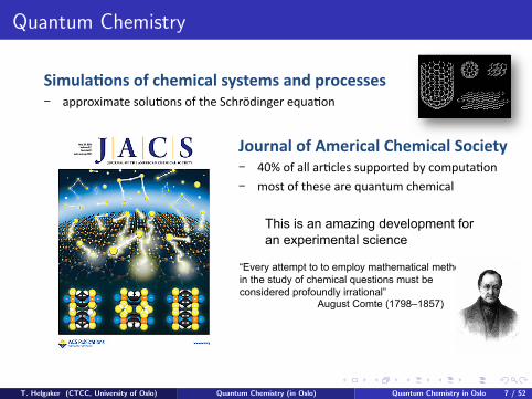
Quantum Chemistry!"#$%"&'()*&+,%-.'

/+&"0#12$,'23'()*&+(#0',.,%*&,'#$4'5-2(*,,*,'

!! !""#$%&'!()*+$,-.$/+*$0*(1)*231#45&/6)#*)7-!.$/*

62"-$#0'23'7&*-+(#0'8)*&+(#0'/2(+*%.'

!! 89:*$0*!,,*!#.3,)+*+-""$#()5*;<*3$'"-(!.$/*

!! '$+(*$0*(1)+)*!#)*7-!/(-'*31)'&3!,*

=>?@>*

“Every attempt to to employ mathematical methods

in the study of chemical questions must be

considered profoundly irrational” August Comte (1798–1857)

This is an amazing development for

an experimental science


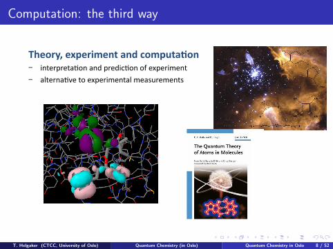
Computation: the third way!"#$%&'(")*+&,-+&,./0+1'2+

3,-"/24+-5$-/.#-)&+')0+6"#$%&'(")+

!! !"#$%&%$#'()"*'"+*&%$+!,()"*)-*$.&$%!/$"#*

!! '0#$%"'(1$*#)*$.&$%!/$"#'0*/$'23%$/$"#2*

45675*


Computer usage NOTUR 2007!"#$%&'()%*+,')-"&%().//0)


Quantum chemistry

I Chemical systems are difficult many-body problems

I with modern computers, the molecular many-body problem has become tractable

I Today, a large number of chemical problems have become amenable to calculation:

I molecular structure and spectroscopic constantsI reaction enthalpies and equilibrium constantsI reactivity, reaction rates, and dynamicsI interaction with applied electromagnetic fields and radiation

I Nowadays, quantum-chemical calculations are routinely carried out by nonspecialists:

I computation constitutes about one quarter of all chemical researchI we are number crunchers

I Quantum chemistry has been responsible for many qualitative models in chemistry

I such models are good and usefulI however, they do not constitute the bread and butter of quantum chemistry

I Quantum chemists must provide tools that compete with experiment

I ideally, our results should be as accurate as experiment: chemical accuracyI if we cannot consistently provide high accuracy, we will be out of business


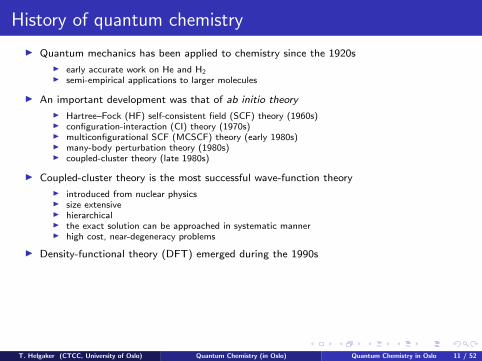
History of quantum chemistry

I Quantum mechanics has been applied to chemistry since the 1920s

I early accurate work on He and H2I semi-empirical applications to larger molecules

I An important development was that of ab initio theory

I Hartree–Fock (HF) self-consistent field (SCF) theory (1960s)I configuration-interaction (CI) theory (1970s)I multiconfigurational SCF (MCSCF) theory (early 1980s)I many-body perturbation theory (1980s)I coupled-cluster theory (late 1980s)

I Coupled-cluster theory is the most successful wave-function theory

I introduced from nuclear physicsI size extensiveI hierarchicalI the exact solution can be approached in systematic mannerI high cost, near-degeneracy problems

I Density-functional theory (DFT) emerged during the 1990s


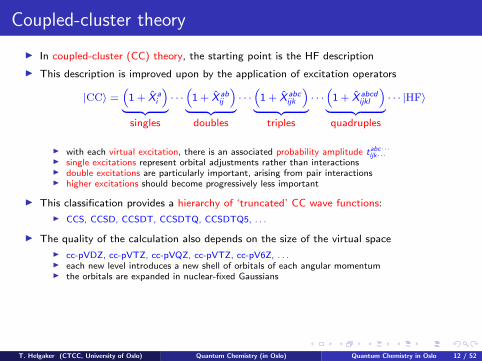
Coupled-cluster theory

I In coupled-cluster (CC) theory, the starting point is the HF description

I This description is improved upon by the application of excitation operators

|CC〉 =“

1 + X ai

”| {z }

singles

· · ·“

1 + X abij

”| {z }

doubles

· · ·“

1 + X abcijk

”| {z }

triples

· · ·“

1 + X abcdijkl

”| {z }quadruples

· · · |HF〉

I with each virtual excitation, there is an associated probability amplitude tabc···ijk···

I single excitations represent orbital adjustments rather than interactionsI double excitations are particularly important, arising from pair interactionsI higher excitations should become progressively less important

I This classification provides a hierarchy of ‘truncated’ CC wave functions:

I CCS, CCSD, CCSDT, CCSDTQ, CCSDTQ5, . . .

I The quality of the calculation also depends on the size of the virtual space

I cc-pVDZ, cc-pVTZ, cc-pVQZ, cc-pVTZ, cc-pV6Z, . . .I each new level introduces a new shell of orbitals of each angular momentumI the orbitals are expanded in nuclear-fixed Gaussians


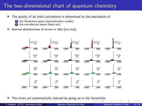
The two-dimensional chart of quantum chemistry

I The quality of ab initio calculations is determined by the description of

1 the N-electron space (wave-function model);2 the one-electron space (basis set).

I Normal distributions of errors in AEs (kJ/mol)

-200 200

HFDZ

-200 200 -200 200

HFTZ

-200 200 -200 200

HFQZ

-200 200 -200 200

HF5Z

-200 200 -200 200

HF6Z

-200 200

-200 200

MP2DZ

-200 200 -200 200

MP2TZ

-200 200 -200 200

MP2QZ

-200 200 -200 200

MP25Z

-200 200 -200 200

MP26Z

-200 200

-200 200

CCSDDZ

-200 200 -200 200

CCSDTZ

-200 200 -200 200

CCSDQZ

-200 200 -200 200

CCSD5Z

-200 200 -200 200

CCSD6Z

-200 200

-200 200

CCSD(T)DZ

-200 200 -200 200

CCSD(T)TZ

-200 200 -200 200

CCSD(T)QZ

-200 200 -200 200

CCSD(T)5Z

-200 200 -200 200

CCSD(T)6Z

-200 200

I The errors are systematically reduced by going up in the hierarchies


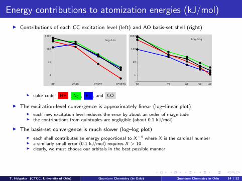
Energy contributions to atomization energies (kJ/mol)

I Contributions of each CC excitation level (left) and AO basis-set shell (right)

HF CCSD CCSDT CCSDTQ

1

10

100

1000

Log!Lin

DZ TZ QZ 5Z 6Z

1

10

100

1000Log!Log

I color code: HF , N2 , F2 , and CO

I The excitation-level convergence is approximately linear (log–linear plot)

I each new excitation level reduces the error by about an order of magnitudeI the contributions from quintuples are negligible (about 0.1 kJ/mol)

I The basis-set convergence is much slower (log–log plot)

I each shell contributes an energy proportional to X−4 where X is the cardinal numberI a similarly small error (0.1 kJ/mol) requires X > 10I clearly, we must choose our orbitals in the best possible manner


Coupled-cluster convergence

Bond distances (pm)

RHF SD T Q 5 rel. theory exp. err.HF 89.70 1.67 0.29 0.02 0.00 0.01 91.69 91.69 0.00N2 106.54 2.40 0.67 0.14 0.03 0.00 109.78 109.77 0.01F2 132.64 6.04 2.02 0.44 0.03 0.05 141.22 141.27 −0.05CO 110.18 1.87 0.75 0.04 0.00 0.00 112.84 112.84 0.00

Harmonic vibrational constants ωe (cm−1)

RHF SD T Q 5 rel. theory exp. err.HF 4473.8 −277.4 −50.2 −4.1 −0.1 −3.5 4138.5 4138.3 0.2N2 2730.3 −275.8 −72.4 −18.8 −3.9 −1.4 2358.0 2358.6 −0.6F2 1266.9 −236.1 −95.3 −15.3 −0.8 −0.5 918.9 916.6 2.3CO 2426.7 −177.4 −71.7 −7.2 0.0 −1.3 2169.1 2169.8 0.7


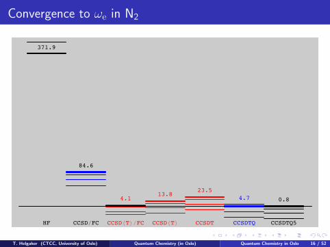
Convergence to ωe in N2

371.9

84.6

4.113.8

23.54.7 0.8

HF CCSD!FC CCSD"T#!FC CCSD"T# CCSDT CCSDTQ CCSDTQ5


The emergence of DFT

I The traditional methods of quantum chemistry are capable of high accuracyI nevertheless, most calculations are performed using density-functional theory (DFT)

I What is the reason for the poularity of DFT?I the standard methods are (at least for high accuracy) very expensive


Density-functional theory

I In chemistry, we view the electronic energy as a functional Eλ[v ] of the potential

v(r) =P

KZKrK

Coulomb potential

I The ground-state energy with external potential v and coupling strength λ:

Eλ[v ] = infΨ→N

˙Ψ˛Hλ[v ]

˛Ψ¸

Hλ[v ] = T + λW +P

i v(ri ), W =P

i>j r−1ij , 0 ≤ λ ≤ 1

I It is possible to perform this minimization in two steps

Eλ[v ] = infρ→N

“Fλ[ρ] +

Rv(r)ρ(r) dr

”Hohenberg–Kohn variation principle

Fλ[ρ] = infΨ→ρ

˙Ψ˛Hλ[0]

˛Ψ¸

Levy constrained-search functional

I The universal density functional Fλ[ρ] depends only on the density

I the density depends only on three spatial coordinatesI no need for the wave function?

I However, the form of Fλ[ρ] is unknown

I In applications of DFT, parametrized approximations to Fλ[ρ] are made

I typically assessed by comparison with experiment

T. Helgaker (CTCC, University of Oslo) The universal density functional and Lieb’s theory Quantum Chemistry in Oslo 18 / 52

The Lieb convex-conjugate functional

I In Lieb’s theory (1983), Fλ[ρ] is defined as the convex conjugate to Eλ[v ]:

Fλ[ρ] = supv

`Eλ[v ]−

Rv(r)ρ(r) dr

´the Lieb variation principle

Eλ[v ] = infρ

`Fλ[ρ] +

Rv(r)ρ(r) dr

´the Hohenberg–Kohn variation principle

I the two variation principles are Legendre–Fenchel (LF) transforms

I The possibility of the LF formulation follows from the convexity of −Eλ[v ] in v :

x1 x2

f!x1"f!x2"

c f!x1"!!1"c" f!x2"f!x2"

c x1!!1"c"x2

f!c x1!!1"c"x2"

I it then has a convex conjugate partner: the Lieb functional Fλ[ρ]I conjugate functions have inverse first derivatives

I A convex functional and its conjugate partner satisfy Fenchel’s inequality:

Fλ[ρ] ≥ Eλ[v ]−R

v(r)ρ(r) dr ⇔ Eλ[v ] ≤ Fλ[ρ] +R

v(r)ρ(r) dr

I either variation principle sharpens Fenchel’s inequality into an equality


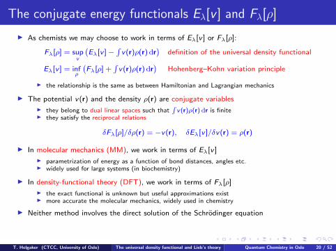
The conjugate energy functionals Eλ[v ] and Fλ[ρ]

I As chemists we may choose to work in terms of Eλ[v ] or Fλ[ρ]:

Fλ[ρ] = supv

`Eλ[v ]−

Rv(r)ρ(r) dr

´definition of the universal density functional

Eλ[v ] = infρ

`Fλ[ρ] +

Rv(r)ρ(r) dr

´Hohenberg–Kohn variation principle

I the relationship is the same as between Hamiltonian and Lagrangian mechanics

I The potential v(r) and the density ρ(r) are conjugate variables

I they belong to dual linear spaces such thatR

v(r)ρ(r) dr is finiteI they satisfy the reciprocal relations

δFλ[ρ]/δρ(r) = −v(r), δEλ[v ]/δv(r) = ρ(r)

I In molecular mechanics (MM), we work in terms of Eλ[v ]

I parametrization of energy as a function of bond distances, angles etc.I widely used for large systems (in biochemistry)

I In density-functional theory (DFT), we work in terms of Fλ[ρ]

I the exact functional is unknown but useful approximations existI more accurate the molecular mechanics, widely used in chemistry

I Neither method involves the direct solution of the Schrodinger equation


Lieb’s theory for approximate energies

I Lieb’s theory may be applied to any exact or approximate energy that is concave:

Fmodλ [ρ]

LF←→ Emodλ [v ]

I examples: the lowest state of any spin symmetryI examples: all variationally determined energies such as EHF

λ [v ] and EFCIλ [v ]

I For nonconcave energies, Fmodλ [ρ] is well-defined but not strictly conjugate to Emod

λ [v ]

I instead, Fmodλ [ρ] is conjugate to the least concave upper bound to the energy

Emodλ [v ]

LF−→ F modλ [ρ]

LF←→ eEmodλ [v ] ≥ Emod

λ [v ]

!4 !2 2 4

!2

!1

1

2

3

4

!4 !2 2 4

!2

!1

1

2

3

4

I examples: EMP2λ [v ] and ECCSD

λ [v ]

T. Helgaker (CTCC, University of Oslo) Approximate energies Quantum Chemistry in Oslo 21 / 52

Kohn–Sham theory

I Density-functional theory in a nutshell:

Eλ[v ] = infρ→N

“Fλ[ρ] +

Rv(r)ρ(r) dr

”Hohenberg–Kohn variation principle

Fλ[ρ] = infΨ→ρ

˙Ψ˛T + λW

˛Ψ¸

universal density functional

I the universal density functional is an unknown quantity, the kinetic energy being most difficult

I Let us relate it to the corresponding noninteracting quantity:

Fλ[ρ] = F0[ρ] +

Z λ

0F ′λ[ρ] dλ = Ts[ρ] + λJ[ρ] + Exc,λ[ρ]

where

Ts[ρ] = F0[ρ] = infΨ→ρ

˙Ψ˛T˛Ψ¸

noninteracting kinetic energy

J[ρ] =

ZZρ(r1)ρ(r2)r−1

12 dr1dr2 Coulomb energy

Exc,λ[ρ] = Fλ[ρ]− Ts[ρ]− λJ[ρ] exchange–correlation energy

I A noninteracting system can be solved exactly, at low cost, by introducing orbitals

ρ(r) =X

iφi (r)

∗φi (r)

I In Kohn–Sham theory, we solve a noninteracting problem in an effective potentialˆ− 1

2∇2 + veff(r)

˜φi (r) = εiφi (r), veff(r) = v(r) + vJ(r) + δExc[ρ]

δρ(r)

I veff(r) is adjusted such that the noninteracting density is equal to the truedensity

I it remains to specify the exchange–correlation functional Exc[ρ]


The exchange–correlation functional

I The exact exchange–correlation functional is unknown

I we must rely on approximations

I Local-density approximation (LDA)

I XC functional modeled after the uniform electron gas (which is known exactly)

ELDAxc [ρ] =

Zf (ρ(r)) dr local dependence on density

I widely applied in condensed-matter physicsI not sufficiently accurate to compete with traditional methods of quantum chemistry

I Generalized-gradient approximation (GGA)

I introduce a dependence also on the density gradient

EGGAxc [ρ] =

Zf (ρ(r,∇ρ(r)) dr local dependence on density and its gradient

I Becke’s gradient correction to exchange (1988) changed the situationI the accuracy became sufficient to compete in chemistryI indeed, surprisingly high accuracy for energetics


Exchange–correlation functionals (plural)

I The exchange–correlation energy contains several contributions

Exc[ρ] = F [ρ]− Ts[ρ]− J[ρ]

I exchange (dominant), correlation, kinetic-energy correction

I The Dirac exchange with Becke’s gradient correction:

EX =Pσ

Rρσ`EDiracσ (r) + EBecke

σ (r)´dr

EDiracσ (r) = − 3

4

`6π

´1/3ρ

1/3σ (r)

EBeckeσ (r) = − βρ

1/3σ (r)s2

σ(r)

1+6βsσ(r) sinh−1 sσ(r), sσ(r) =

|∇ρσ(r)|ρ

4/3σ (r)

I the Becke correction contains the adjustable parameter β = 0.0042I fitted to HF exchange of noble-gas atoms

I The Becke correction is often used with the LYP (Lee–Yang–Parr) correlation functional

I contains four adjustable parameters, fitted to the helium-atom correlation energy

I The resulting functional is known under the acronym BLYP

I a bewildering variety of functionals has been developedI sometimes chosen to satisfy exact conditions, other times fitted to data


Hybrid DFT

I We have already introduced orbitals to evaluate the kinetic energy

I why not use the orbitals to evaluate the exact HF exchange?I this is both a good and bad idea . . .

I The replacement of functional exchange with exact exchange makes things worse

I at least for energetics...I it is difficult to find a correlation functional to match exact exchangeI this has to do with the delocalization of the exact exchange hole

I However, some proportion of exact exchange is a good thing for energetics

I in B3LYP, 20% is used: good for energeticsI this has for many years been the most popular functional

I For other properties, 100% exact exchange is better. . .

I polarizabilities, excitation energies

I Attempts have been made to use orbitals in a variety of manners

I dispersion is not described by local and semi-local functionalsI traditional quantum chemistry describes dispersion wellI elements of MP2 introduced into DFT


A plethora of exchange–correlation functionals

exchange, Slater local exchange, and the nonlocal gradientcorrection of Becke88. Thus,

ExcB3LYP ! a0Ex

exact " !1 # a0"ExSlater " ax#Ex

B88 " acEcVWN

" !1 # ac"EcLYP. [11]

Becke obtained the hybrid parameters {a0, ax, ac} $ {0.20, 0.72,0.19} (3) from a least-squares fit to 56 atomization energies, 42IPs, and 8 proton affinities (PAs) of the G2-1 set of atoms andmolecules (4). B3LYP leads to excellent thermochemistry (0.13eV MAD) and structures for covalently systems but does notaccount for London dispersion (all noble gas dimers are pre-dicted unstable).

Following B3LYP, we introduce the extended hybrid func-tional, denoted as X3LYP:

ExcX3LYP ! a0Ex

exact " !1 # a0"ExSlater " ax#Ex

X " acEcVWN

" !1 # ac"EcLYP. [12]

We determined the hybrid parameters {a0, ax, ac} $ {0.218,0.709, 0.129} in X3LYP just as for XLYP. Thus, we normalizedthe mixing parameters of Eq. 10 and redetermined {ax1, ax2} ${0.765, 0.235} for X3LYP. The FX(s) function of X3LYP (Fig.1) agrees with FGauss(s) for larger s.

Results and DiscussionWe tested the accuracy of XLYP and X3LYP for a broad rangeof systems and properties not used in fitting the parameters.Table 1 compares the overall performance of 17 different flavorsof DFT methods, showing that X3LYP is the best or nearly best

Table 1. MADs (all energies in eV) for various level of theory for the extended G2 set

Method

G2(MAD)

H-Ne, Etot TM #E He2, #E(Re) Ne2, #E(Re) (H2O)2, De(RO . . . O)#Hf IP EA PA

HF 6.47 1.036 1.158 0.15 4.49 1.09 Unbound Unbound 0.161 (3.048)G2 or best ab initio 0.07a 0.053b 0.057b 0.05b 1.59c 0.19d 0.0011 (2.993)e 0.0043 (3.125)e 0.218 (2.912)f

LDA (SVWN) 3.94a 0.665 0.749 0.27 6.67 0.54g 0.0109 (2.377) 0.0231 (2.595) 0.391 (2.710)GGA

BP86 0.88a 0.175 0.212 0.05 0.19 0.46 Unbound Unbound 0.194 (2.889)BLYP 0.31a 0.187 0.106 0.08 0.19 0.37g Unbound Unbound 0.181 (2.952)BPW91 0.34a 0.163 0.094 0.05 0.16 0.60 Unbound Unbound 0.156 (2.946)PW91PW91 0.77 0.164 0.141 0.06 0.35 0.52 0.0100 (2.645) 0.0137 (3.016) 0.235 (2.886)mPWPWh 0.65 0.161 0.122 0.05 0.16 0.38 0.0052 (2.823) 0.0076 (3.178) 0.194 (2.911)PBEPBEi 0.74i 0.156 0.101 0.06 1.25 0.34 0.0032 (2.752) 0.0048 (3.097) 0.222 (2.899)XLYPj 0.33 0.186 0.117 0.09 0.95 0.24 0.0010 (2.805) 0.0030 (3.126) 0.192 (2.953)

Hybrid methodsBH & HLYPk 0.94 0.207 0.247 0.07 0.08 0.72 Unbound Unbound 0.214 (2.905)B3P86l 0.78a 0.636 0.593 0.03 2.80 0.34 Unbound Unbound 0.206 (2.878)B3LYPm 0.13a 0.168 0.103 0.06 0.38 0.25g Unbound Unbound 0.198 (2.926)B3PW91n 0.15a 0.161 0.100 0.03 0.24 0.38 Unbound Unbound 0.175 (2.923)PW1PWo 0.23 0.160 0.114 0.04 0.30 0.30 0.0066 (2.660) 0.0095 (3.003) 0.227 (2.884)mPW1PWp 0.17 0.160 0.118 0.04 0.16 0.31 0.0020 (3.052) 0.0023 (3.254) 0.199 (2.898)PBE1PBEq 0.21i 0.162 0.126 0.04 1.09 0.30 0.0018 (2.818) 0.0026 (3.118) 0.216 (2.896)O3LYPr 0.18 0.139 0.107 0.05 0.06 0.49 0.0031 (2.860) 0.0047 (3.225) 0.139 (3.095)X3LYPs 0.12 0.154 0.087 0.07 0.11 0.22 0.0010 (2.726) 0.0028 (2.904) 0.216 (2.908)Experimental — — — — — — 0.0010 (2.970)t 0.0036 (3.091)t 0.236u (2.948)v

#Hf, heat of formation at 298 K; PA, proton affinity; Etot, total energies (H-Ne); TM #E, s to d excitation energy of nine first-row transition metal atoms andnine positive ions. Bonding properties [#E or De in eV and (Re) in Å] are given for He2, Ne2, and (H2O)2. The best DFT results are in boldface, as are the most accurateanswers [experiment except for (H2O)2].aRef. 5.bRef. 19.cRef. 4.dRef. 35.eRef. 38.fRef. 34.gRef. 37.hRef. 7.iRef. 10.j1.0 Ex (Slater) % 0.722 #Ex (B88) % 0.347 #Ex (PW91) % 1.0 Ec (LYP).k0.5 Ex (HF) % 0.5 Ex (Slater) % 0.5 #Ex (B88) % 1.0 Ec (LYP).l0.20 Ex (HF) % 0.80 Ex (Slater) % 0.72 #Ex (B88) % 1.0 Ec (VWN) % 0.81 #Ec (P86).m0.20 Ex (HF) % 0.80 Ex (Slater) % 0.72 #Ex (B88) % 0.19 Ec (VWN) % 0.81 Ec (LYP).n0.20 Ex (HF) % 0.80 Ex (Slater) % 0.72 #Ex (B88) % 1.0 Ec (PW91, local) % 0.81 #Ec (PW91, nonlocal).o0.25 Ex (HF) % 0.75 Ex (Slater) % 0.75 #Ex (PW91) % 1.0 Ec (PW91).p0.25 Ex (HF) % 0.75 Ex (Slater) % 0.75 #Ex (mPW) % 1.0 Ec (PW91).q0.25 Ex (HF) % 0.75 Ex (Slater) % 0.75 #Ex (PBE) % 1.0 Ec (PW91, local) % 1.0 #Ec (PBE, nonlocal).r0.1161 Ex (HF) % 0.9262 Ex (Slater) % 0.8133 #Ex (OPTX) % 0.19 Ec (VWN5) % 0.81 Ec (LYP).s0.218 Ex (HF) % 0.782 Ex (Slater) % 0.542 #Ex (B88) % 0.167 #Ex (PW91) % 0.129 Ec (VWN) % 0.871 Ec (LYP).tRef. 27.uRef. 33.vRef. 32.

Xu and Goddard PNAS ! March 2, 2004 ! vol. 101 ! no. 9 ! 2675

CHEM

ISTR

Y


Reaction Enthalpies (kJ/mol)

B3LYP CCSD(T) exp.CH2 + H2 → CH4 −543 1 −543 1 −544(2)C2H2 + H2 → C2H4 −208 −5 −206 −3 −203(2)C2H2 + 3H2 → 2CH4 −450 −4 −447 −1 −446(2)CO + H2 → CH2O −34 −13 −23 −2 −21(1)N2 + 3H2 → 2NH2 −166 −2 −165 −1 −164(1)F2 + H2 → 2HF −540 23 −564 −1 −563(1)O3 + 3H2 → 3H2O −909 24 −946 −13 −933(2)CH2O + 2H2 → CH4 + H2O −234 17 −250 1 −251(1)H2O2 + H2 → 2H2O −346 19 −362 3 −365(2)CO + 3H2 → CH4 + H2O −268 4 −273 −1 −272(1)HCN + 3H2 → CH4 + NH2 −320 0 −321 −1 −320(3)HNO + 2H2 → H2O + NH2 −429 15 −446 −2 −444(1)CO2 + 4H2 → CH4 + 2H2O −211 33 −244 0 −244(1)2CH2 → C2H4 −845 −1 −845 −1 −844(3)


Ab-initio studies of the universal density functional

I Lieb’s theory allows us to study the universal density functional from wave functions

Fλ[ρ] = supv

`Eλ[v ]−

Rv(r)ρ(r) dr

´the Lieb variation principle

Eλ[v ] = infρ

`Fλ[ρ] +

Rv(r)ρ(r) dr

´the Hohenberg–Kohn variation principle

I we have recently implemented Lieb’s variation principleI first such implementation beyond small 2- and 4-electron atomsI Andy Teale and Sonia Coriani

I The Lieb variation principle provides a new tool for DFTI benchmark excisting functionalsI develop new ones

I We expand the potential v in simple functions and determine the coefficients

vc(r) = vext(r) + (1− λ)vref(r) +X

t

ct gt(r)

I Kohn–Sham decomposition of the exchange–correlation functional:

Fλ[ρ] = F0[ρ] +

Z λ

0F ′λ[ρ] dλ = Ts[ρ] + λJ[ρ] + Exc,λ[ρ]

I this is the adiabatic connnection

I We express the XC functional by integration over λ:

Exc,λ[ρ] =

Z λ

0Wλ[ρ] dλ


The adiabatic connection: the dissociation of H2

I To study static correlation, we consider H2 dissociationI RHF, BLYP, and FCI levels of theory in the aug-cc-pVQZ basis

2 4 6 8-1.2

-1.1

-1.0

-0.9

-0.8

-0.7

-0.6

-0.5

FCI

BLYP

HF


Adiabatic connection: XC curves for H2R = 0.7 bohr

I At short distances, exchange (−0.827Eh) dominates over correlation (−0.039Eh) energy

I BLYP curve performs well, reproducing HF exchange and FCI correlation

I The BLYP and CI curves are nearly linear, indicative of dynamical correlation

0.0 0.2 0.4 0.6 0.8 1.0

-0.9

-0.8

-0.7

-0.6

-0.5

-0.4

R = 0.7 bohrFCI

BLYP

HF



I The overall picture is similar to that at R = 0.7 bohr

I Most notably, the exchange energy decreases in magnitude from −827 to −661 mEh

I The correlation energy increases slightly in magnitude, from −39 to −41 mEh

0.0 0.2 0.4 0.6 0.8 1.0

-0.9

-0.8

-0.7

-0.6

-0.5

-0.4

R = 1.4 bohr

FCI

BLYP

HF



I The exchange energy decreases further in magnitude from −661 to −477 mEh

I The correlation energy increases in magnitude from −41 to −77 mEh

I The FCI curve now curves more strongly, indicative of static correlation

I The BLYP functional overestimates exchange but works well by LYP error cancellation

0.0 0.2 0.4 0.6 0.8 1.0

-0.9

-0.8

-0.7

-0.6

-0.5

-0.4

R = 3.0 bohr

FCI

BLYP

HF



I The overall picture is similar to that at R = 3.0 bohr

I However, the static-correlation curvature of the FCI curve is now more pronounced

I The (nonconvex) BLYP curve strongly underestimates the magnitude of the XC energy

I The BLYP curve now benefits less from error cancellation

0.0 0.2 0.4 0.6 0.8 1.0

-0.9

-0.8

-0.7

-0.6

-0.5

-0.4

R = 5.0 bohr

FCI

BLYP

HF



I At R = 10 bohr, the two atoms are separated and correlation is essentially static

I Dynamical correlation is now less than 1 Eh (dispersion)

I The BLYP functional works mostly by overestimating the exchange energy

I It still has a nonzero slope, indicative of dynamic correlation!

0.0 0.2 0.4 0.6 0.8 1.0

-0.9

-0.8

-0.7

-0.6

-0.5

-0.4

R =10.0 bohr

FCI

BLYP

HF


A two-parameter CI model applied to the H2 moleculeI A better two-parameter model is obtained from a two-level CI model

Eλ,c[ρ] =1

2∆E −

1

2

p∆E 2 + 4w2λ2, ∆E = h + gλ

Wλ,c[ρ] =1

2g −

g(h + gλ) + 4w2λ

2p

(h + gλ)2 + 4w2λ2

I excellent least-square fits with two adjustable parametersI good fits to initial gradient and end point

0.0 0.2 0.4 0.6 0.8 1.0

-0.25

-0.20

-0.15

-0.10

-0.05

0.00

Λ

Wc,

Λ�

a.u.

R = 0.7 a.u.

R = 1.4 a.u.

R = 3.0 a.u.

R = 5.0 a.u.

R = 7.0 a.u.

R = 10.0 a.u.


Molecular properties

I Over the last decade, DFT has become the workhorse of chemistry

I its popularity stems from its ability to provide good structures and energetics

I DFT is widely used also for molecular properties

I response theoryI geometric, electric, magnetic perturbationsI static and dynamic perturbationsI linear and nonlinear response

I For most properties, the application of DFT has been a success

I a revolution in the calculation of nuclear spin–spin coupling constants

I Excitation energies are an interesting case

I important chemical property of moleculesI accessible from linear-response theoryI some excitations are well reproduced, others poorlyI the failures highlight deficiencies in the exchange–correlation potential


Response theory

I The expectation value of A in the presence of a perturbation Vω of frequency ω:˙t˛A˛t¸

=˙0˛A˛0¸

+

Z〈〈A; Vω〉〉ω exp (−iωt) dω + · · ·

I the linear-response function 〈〈A; Vω〉〉ωI carries information about the first-order change in the expectation value

I The linear-response function may be represented compactly as:

〈〈A; Vω〉〉ω = −A[1]T È[2] − ωS[2]

´−1V

[1]ω| {z }

linear equations

←

8<: E[2] electronic Hessian

S[2] metric matrix

A[1] = vecÀDS− SDA

Í In practice, the response functions are evaluated by solving a set of linear equations`

E[2] − ωS[2]Ń[1] = −V

[1]ω

〈〈A; Vω〉〉ω = A[1]TN[1]

I Excitation energies as poles of linear response function (RPA):È[2] − ωS[2]

´X = 0


Indirect nuclear spin–spin coupling constants

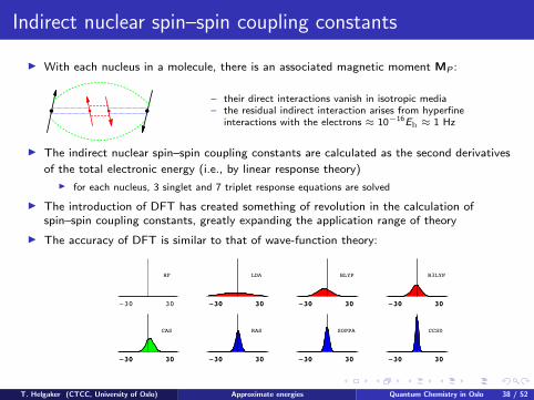
I With each nucleus in a molecule, there is an associated magnetic moment MP :

– their direct interactions vanish in isotropic media– the residual indirect interaction arises from hyperfine

interactions with the electrons ≈ 10−16Eh ≈ 1 Hz

I The indirect nuclear spin–spin coupling constants are calculated as the second derivatives

of the total electronic energy (i.e., by linear response theory)

I for each nucleus, 3 singlet and 7 triplet response equations are solved

I The introduction of DFT has created something of revolution in the calculation ofspin–spin coupling constants, greatly expanding the application range of theory

I The accuracy of DFT is similar to that of wave-function theory:

!30 30

CAS

!30 30 !30 30

RAS

!30 30 !30 30

SOPPA

!30 30 !30 30

CCSD

!30 30

!30 30

HF

!30 30

LDA

!30 30 !30 30

BLYP

!30 30 !30 30

B3LYP

!30 30


NMR spectra: nuclear magnetic spin transitions

I Effective NMR spin Hamiltonian

H = −X

i

BT(I− σi )Miz +Xi<j

KijMi ·Mj

σi = d2E/dBdMi , Kij = d2E/dMidMj

I Simulated 200 MHz NMR spectra of vinyllithium (C2H3Li)

0 100 200

MCSCF

0 100 200 0 100 200

B3LYP

0 100 200

0 100 200

experiment

0 100 200 0 100 200

RHF

0 100 200


Valinomycin C54H90N8O18

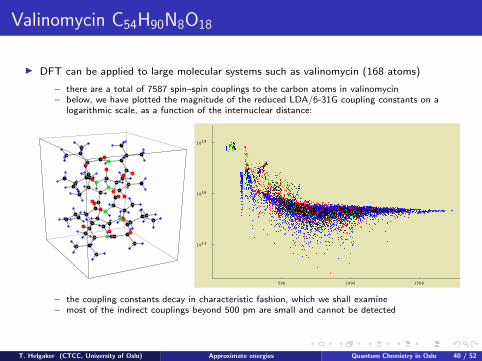
I DFT can be applied to large molecular systems such as valinomycin (168 atoms)

– there are a total of 7587 spin–spin couplings to the carbon atoms in valinomycin– below, we have plotted the magnitude of the reduced LDA/6-31G coupling constants on a

logarithmic scale, as a function of the internuclear distance:

500 1000 1500

1019

1016

1013

– the coupling constants decay in characteristic fashion, which we shall examine– most of the indirect couplings beyond 500 pm are small and cannot be detected


Dalton Program System


Towards large systems!"#$%&'()$%*+%(','-+.'/(

•! !"#$%&'($)*+(',$"-.*#("*/0+12#$$0*$#(3"*–! 2'-+4/#5'6#$*2'./*/0+12#$$0*.2#$".*24,12#$$0*'(*7137*&1/7*162("#.163*.0./"-*.18"*

–! 7'&"9"(:*16*$#(3"*.0./"-.:*6"#($0*#$$*2'6/(1,45'6.*#("*16.1361;2#6/*

–! /7"."*.7'4$)*,"*("2'3618")*#6)*#9'1)")*16*/7"*2'-+4/#5'6.*

–! 1)"#$$0:*2'./*.7'4$)*162("#."*16*+('+'(5'6*/'*.0./"-*.18"*


BP86/6-31G** KS matrix in linear polyene chains

æ æ ææ

æ

à

à

à

à

à

ì

ì

ì

ì

ì

ò

ò

ò

ò

ò

ô ôô

ôô

50 100 150 200 2500

10

20

30

40

Number of carbons

Tim

eHsL

NF

FF

Linsol

XC


BP86/6-31G** gradient in linear polyene chains

0

5

10

15

20

25

30

35

40

45

50

0 50 100 150 200 250

XCONENF-JFF-J


Example: titin molecule

Proteins under external load

Structure optimized at PB86/6-31g (S:6-31g(d))

Titin Model Protein [4]

[4] Liang, J. And Fernandex, J. M., ACS Nano, 3 (7), (2009)

I 392 atoms, BP86, 6-31G/Ahlrichs-Coulomb-Fit w/ 6-31G* on 5 atoms

I Total timings each SCF iteration: KS-matrix 4–6 m; RH/DIIS 30 s

I Total timings each geometry step: RH/DIIS energy 1 h 10 m; forces 9 m

I Francesca Iozzi, Andreas Krapp, Patrick Merlot, Simen Reine


Molecules in finite magnetic fields

I New code (LONDON) for calculations in finite magnetic fields

I London orbitals: hybrid plane-wave-Gaussian (PWG) orbitals

ωκ,c (r) = exp(iκ · r)| {z }plane wave

Slm(r) exp(−ar2A)| {z }

solid-harmonic Gaussian

I mixed basis for periodic boundary conditions and scattering studies

I gauge-origin independent magnetic properties at zero field

I McMurchie–Davidson PWG screened developed and implemented

I Erik Tellgren and Alessandro Soncini

æ

æ

æ

æ

æ

æ

æ

æ

æ

æ

æ

æ

æ

æ

æ

æ

æ

æ

æ

ææ

ææææææææææææææ

ææ

æææææ

ææææææææææææææ

ææ

æææææææææææ

æææ

ææ

æ

æ

æ

æ

æ

æ

æ

æ

æ

æ

æ

æ

æ

æ

æ

æ

æ

æ

æ

-0.04 -0.02 0.02 0.04

-756.710

-756.705

-756.700

-756.695

-756.690

-756.685

-756.680


F2 potential-energy curve in a perpendicular magnetic field

I The magnetic field changes the shape of the potential-energy curve

2.5 3.0 3.5 4.0 4.5 5.0 5.5

-198.7

-198.6

-198.5

-198.4

B=0.00

B=0.05

B=0.10

B=0.45

B=0.30

I diamagnetic behaviour in the molecular limitI paramagnetic behaviour in the atomic limit

I The bond length of F2 increases with increasing magnetic field


Computational Chemistry

I We are chemists!

I Apply existing quantum chemical methodology to chemical relevant questions

I Close collaboration with experimentalists

I to analyze experimental resultsI to get ideas for new experiments

I Two recent examples from UiO collaborations


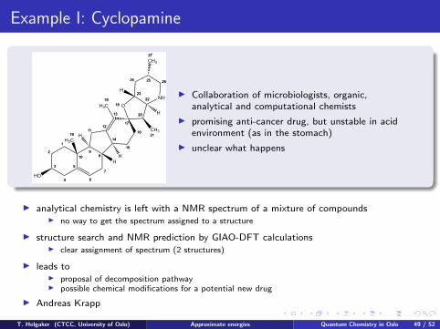
Example I: Cyclopamine

33

44

55

1010

11

22

66

77

88

99

1414

1212

1111

1515

1616

1717

1313

O1818

2323

2222

2020

2424 2525 2626

NH

CH3

2727

HO

H

H3C

1818

H

H

H3C

1919

H

CH32121H

I Collaboration of microbiologists, organic,analytical and computational chemists

I promising anti-cancer drug, but unstable in acidenvironment (as in the stomach)

I unclear what happens

I analytical chemistry is left with a NMR spectrum of a mixture of compoundsI no way to get the spectrum assigned to a structure

I structure search and NMR prediction by GIAO-DFT calculationsI clear assignment of spectrum (2 structures)

I leads toI proposal of decomposition pathwayI possible chemical modifications for a potential new drug

I Andreas Krapp


Example II: Organometallic catalysis

I observation of specific selectivity of a catalyst: why?

I mapping of the important parts of the potential energy hypersurface

I selectivity determining step located

I leads to molecular understanding of reaction process and ideas for modifications

I Andreas Krapp


Other work in our group

I molecular dynamics (Volodya Rybkin, Vebjørn Bakken)

I finite-element calculation of Coulomb interactions (Michael Przybytek)

I periodic boundary conditions (Johannes Rekkedal, Thomas Bondo Pedersen)

I range-separated DFT (Francesca Iozzi, Andy Teale)


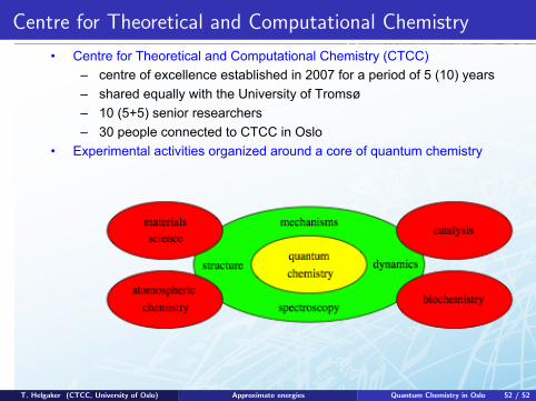
Centre for Theoretical and Computational Chemistry

QSD & CTCC, Department of Chemistry, University of Oslo

•! Centre for Theoretical and Computational Chemistry (CTCC)

–! centre of excellence established in 2007 for a period of 5 (10) years

–! shared equally with the University of Tromsø

–! 10 (5+5) senior researchers

–! 30 people connected to CTCC in Oslo

•! Experimental activities organized around a core of quantum chemistry


quantum chemistry (in oslo) -...

Documents