quantum corrections to thermopower and conductivity in graphene

PHYSICAL REVIEW B 89, 075411 (2014)

Quantum corrections to thermopower and conductivity in graphene

Aleksander P. Hinz* and Stefan Kettemann†

School of Engineering and Science, Jacobs University Bremen, Bremen 28759, Germanyand Asia Pacific Center for Theoretical Physics (APCTP) and Division of Advanced Materials Science, Pohang University of Science

and Technology (POSTECH), San31, Hyoja-dong, Nam-gu, Pohang 790-784, South Korea

Eduardo R. Mucciolo‡

Department of Physics, University of Central Florida, Orlando, Florida 32816-2385, USA(Received 12 April 2013; revised manuscript received 16 January 2014; published 11 February 2014)

The quantum corrections to the conductivity and thermopower in monolayer graphene are studied. We usethe recursive Green’s-function method to calculate numerically the conductivity and thermopower of graphene.We then analyze these weak-localization corrections by fitting with the analytical theory as a function of theimpurity parameters and gate potential. As a result of the quantum corrections to the thermopower, we findlarge magnetothermopower, which is shown to provide a very sensitive measure of the size and strength ofthe impurities. We compare these analytical and numerical results with existing experimental measurements ofmagnetoconductance of single-layer graphene and find that the average size and strength of the impurities inthese samples can thereby be determined. We suggest favorable parameter ranges for future measurements of themagnetothermopower.

DOI: 10.1103/PhysRevB.89.075411 PACS number(s): 65.80.Ck, 72.20.Pa, 73.22.Pr

I. INTRODUCTION

Since its synthesis, graphene [1] has attracted a lot of at-tention, both for its novel electronic properties and its possibleapplications. One of the most remarkable aspects is that theweak-localization effect, which is a typical low-temperaturephenomenon due to quantum corrections to the conductivityδσ , can be observed up to a temperature range of 200 Kelvin ingraphene [2,3]. It has been theoretically predicted that the signof these corrections strongly depends on the kind of impuritiesin the graphene sample [4], so that both positive and nega-tive magnetoconductivity, the so-called weak-antilocalizationeffect, can be observed. This effect is well known to occurdue to spin-orbit interaction, even though the latter is typicallyvery weak in graphene. Noting that the graphene lattice iscomposed of two sublattices, one can formulate the sublatticedegree of freedom as an isospin which is strongly coupled tothe momentum. Thereby, any elastic scattering that breaks thegraphene sublattice symmetry is expected to result in weakantilocalization. This is made more complicated, however, bythe fact that there is another discrete degree of freedom ingraphene, i.e., the two degenerate Dirac cones, which cancorrespondingly be formulated by introducing a pseudospinindex. Accordingly, any scattering which mixes these two val-leys can result in yet another change of the sign of the quantumcorrection to the conductivity, and thereby to the restoration ofweak localization. More recently, thermopower S in graphenehas been measured by several groups [5–8]. The classicalthermopower of graphene has been calculated with a rangeof different methods. The experiments show good agreementwith the Mott formula, which corresponds to the leading termof the Sommerfeld expansion at low temperatures and large

*Corresponding author: [email protected]†[email protected]‡[email protected]

gate voltages [9]. Close to the Dirac point, thermopower showsan unusual behavior, being linear in gate voltage, and changingsign. Thus, while usually thermopower is expected to increaseas the Fermi energy, electron density, and thereby conductivityare lowered, in graphene the thermopower becomes smaller asthe Dirac point is approached and the electron density andconductivity are reduced.

The main aims of this paper are, first, to find out if thereare sizable quantum corrections to the thermopower δS ingraphene and whether they are sensitive to weak magneticfields and, second, to present and analyze the combinedanalytical and numerical theory in order to provide the basisfor a more quantitative analysis of experimental results onthe magnetoconductance of graphene. This will allow one tocharacterize samples, in particular the density, strength, andsize of carrier scatterers, more accurately.

We restrict our attention to the diffusion term of thethermopower and do not consider the phonon drag contri-bution, which becomes relevant only at high temperatures.In normal metals, the quantum corrections to the diffusionthermopower are known to be dominated by the weak-localization corrections to the conductivity, yielding δS/S ≈−δσ/σ [10–12]. Thus, when the conductivity is reduced bythe weak-localization correction, the thermopower becomesenhanced. This is expected since the thermopower is knownto increase from a metal towards an insulator. Because ofthe particular electronic properties of graphene, where thesign of the quantum correction can change upon varyingthe gate voltage, it could be expected that these quantumcorrections to thermopower are particularly large in graphene.We therefore determine the strength and the sign of theresulting magnetothermopower and analyze in detail how itchanges with impurity parameters such as range, density, andstrength, and with gate voltage.

This paper is organized as follows. We start in Sec. II witha short introduction to the electronic properties of graphene.

1098-0121/2014/89(7)/075411(21) 075411-1 ©2014 American Physical Society

http://dx.doi.org/10.1103/PhysRevB.89.075411

HINZ, KETTEMANN, AND MUCCIOLO PHYSICAL REVIEW B 89, 075411 (2014)

We introduce the model for the description of the impuritypotential in Sec. III and list the resulting momentum scatteringrates and their dependence on the impurity matrix elements.In Sec. IV A, we give a brief review of transport theory, inparticular the theory of weak-localization corrections to theconductivity and its application to graphene. In Sec. IV B,we review the theory of thermopower and address leadingquantum corrections.

In Sec. V, we present a numerical method to calculate theconductance which is based on the recursive Green’s-functiontechnique (Sec. V B). We introduce the Hamiltonian thatmodels impurities in graphene for the numerical calculationin Sec. V C and relate it in Sec. VI to the impurity modelintroduced in Sec. III. This connection makes it possible todisplay the related transport scattering rates from Secs. IIIand IV as functions of the sample parameter of the numericalmethod (Sec. V), which is done in Sec. VI B.

In Sec. VII, we present the numerical results for theconductance (Sec. VII A) and thermopower (Sec. VII B). InSec. VIII, we analyze the numerical results by fitting them tothe analytical results (Sec. VIII A). In Sec. VIII B, we attemptan ab initio analysis. To this end, we use the relation of thescattering rates to the impurity parameters of the numericalcalculations and insert it in the analytical formulas given inSec. IV. In Sec. VIII C, we present the analytical results forthe quantum corrections to the conductance at zero magneticfield. In Sec. VIII D, we present the results for the quantumcorrections to the thermopower at zero magnetic field and theresulting magnetic field dependence of the thermopower. InSec. IX, we compare the numerical and analytical results withexperimental results on weak-localization corrections to theconductance. Finally, we draw the conclusions and summarizeour results in Sec. X. In Appendix A, the Hamiltonian isgiven in matrix notation. In Appendix B, we present analyticalresults for the magnetoconductance when the warping rate isneglected, 1/τw = 0.

II. ELECTRONIC STRUCTURE OF GRAPHENE

Let us start with a brief review of the electronic propertiesof graphene, introducing the notation used in this paper. Wefollow the convention of McCann and co-workers [4]. For anoverview and comparison of notations, see also [13–16].

Graphene is a two-dimensional layer of carbon atomsarranged in a honeycomb lattice. These carbon atoms areconnected by strong σ bonds with their three neighboringatoms. The corresponding energy bands are filled valencebonds, lying deep below the Fermi energy. The π bond leadsto the formation of a π band, which is exactly half filledin ungated and undoped graphene. Thus, to study transportproperties, we can restrict the model to this π band. The basisof the Bravais lattice consists of two atoms, with each oneforming one sublattice, named A and B sublattice.

The electronic band structure shows two degenerate half-filled cones, which in momentum space are located on thesites of the hexagonal reciprocal lattice. Close to zero energy,i.e., the Dirac points, the dispersion is, in good approximation,linear. Each Dirac cone is part of a sublattice, the K and K′valleys.

Accordingly, the Hamiltonian can be written as a 4 × 4matrix which, close to the Dirac points in linear approximation,becomes

H1 = vF ζ3 ⊗ �σ · �k, (1)

where ζ3 is the diagonal Pauli matrix in K-K′ space, kx and ky

are components of the momentum �k in the plane, and

�σ =(

σ1

σ2

), (2)

with σ1,2 the nondiagonal Pauli matrices in the sublattice (A,B)space. The next correction term to the dispersion is quadraticand given by

H2 = −μ[σ1(k2x − k2

y

)− 2σ2(kxky)]ζ0, (3)

where μ is the parameter of warping, which is given by [17,18]

μ = 3ta20

8. (4)

In this notation, the four-component Bloch states are given by

��T = (�AK,�BK,�BK′ ,�AK′ ). (5)

The Hamiltonian can be more compactly written in the isospinand pseudospin notation, which is particularly convenient forthe purpose of understanding the sign of weak-localizationcorrections to the conductivity. Following the definition ofMcCann and co-authors [4], we set

0 = ζ0 ⊗ σ0, 1 = ζ3 ⊗ σ1, (6)

2 = ζ3 ⊗ σ2, 3 = ζ0 ⊗ σ3, (7)

and

0 = ζ0 ⊗ σ0, 1 = ζ1 ⊗ σ3, (8)

2 = ζ2 ⊗ σ3, 3 = ζ3 ⊗ σ0, (9)

where σi , i = 1,2,3, are the Pauli matrices and σ0 is the identitymatrix in the sublattice (A,B) space, and ζi , i = 1,2,3, are thePauli matrices and ζ0 is the identity matrix in K-K′ space. Thevector of the 4 × 4 matrices, �T = (1,2,3), is the isospinvector referring to the sublattice (A,B) degrees of freedom,and �T = (1,2,3) is the pseudospin vector referring tothe valley (K, K′) degrees of freedom.

In this notation, the Hamiltonian H1 + H2 can be writtenas

H0 = H1 + H2

= vF� · �k︸︷︷︸

Dirac cone

− μ1( � · �k)31( � · �k)1︸︷︷︸Warping correction to the Dirac cone

. (10)

Note that H1 is independent of the pseudospin �, while thewarping term H2 breaks the pseudospin symmetry.

III. IMPURITIES IN GRAPHENE

Disorder can have many different origins in graphene, suchas adatoms and vacancies, while substitutional defects arerather unlikely due to the strength of the σ bonding. For thepurpose of the transport calculations, it is rather convenient toclassify the disorder according to whether it breaks the isospin

075411-2

QUANTUM CORRECTIONS TO THERMOPOWER AND . . . PHYSICAL REVIEW B 89, 075411 (2014)

symmetry (A, B sublattices) or the the pseudospin symmetry(K, K′ valleys). Thus, the Hamiltonian of nonmagnetic disorderhas, in the representation of the pseudospin � and the isospin�, the general form [4]

Himp = I V0,0 (�r) +3∑

i,j=1

ijVi,j (�r) , (11)

where I is the identity matrix. V0,0 (�r) is the part of thedisorder potential which leaves both the isospin and thepseudospin symmetry invariant, while the other terms arebreaking either of these symmetries with the amplitudesVi,j (�r). We note that this disorder Hamiltonian is invariantunder time reversal, � → − � and � → −�, and thus indeeddescribes nonmagnetic disorder. See Appendix A for theexplicit matrix representation of the Hamiltonian.

The corresponding scattering rates in Born approximationare given by

τ−1ij = (πνV 2

i,j

)/�, (12)

where ν is the density of states per spin and valley. We canthus define the total scattering rate as

τ−1 := τ−100 +

∑i,j=1,2,3

τ−1ij . (13)

The intervalley scattering rate is obtained by summing overall matrix elements which couple to the transverse pseudospincomponents 1 and 2, yielding

τ−1i := 4τ−1

⊥⊥′ + 2τ−13⊥ , (14)

where we introduced ⊥ = 1,2 to denote the transverse compo-nents, noting that τ−1

i1 = τ−1i2 =: τ−1

i⊥ and τ−11j = τ−1

2j =: τ−1⊥j ,

since V 21,j = V 2

2,j =: V 2⊥,j and V 2

i,1 = V 2i,2 =: V 2

i,⊥.The intravalley scattering rate is accordingly given by

τ−1z := 2τ−1

⊥3 + τ−133 . (15)

The trigonal warping term in the kinetic energy of grapheneresults in an asymmetry of the dispersion at each valleywith respect to momentum inversion [19], while the totalHamiltonian including both valleys preserves that symmetry.Therefore, the pseudospin is expected to precess in thepresence of the warping term. In the presence of elasticscattering, the pseudospin channels are expected to relaxaccordingly, as in motional narrowing, in proportion to thescattering time τ ,

τ−1w = 2τ

(E2

F μ

�v2

)2

. (16)

IV. TRANSPORT THEORY

A. Weak localization corrections to the conductancein graphene

Quantum corrections to the conductance, the so-calledweak-localization corrections, originate from the quantuminterference of electrons propagating through the sample.On time scales t exceeding the elastic mean free time τ ,electrons move diffusively and their return probability can beenhanced due to the constructive interference of the amplitudes

for propagation on closed diffusion paths, as long as thattime t does not exceed the phase-coherence time τφ(T ). Inthe presence of spin-orbit interaction, the spin precesses asthe electron moves on closed paths, and the phase of theamplitudes for clockwise and anticlockwise propagation nolonger matches, unless the total spin of these two propagationsadds up to zero. This spin singlet channel leads to destructiveinterference and thereby an enhancement of the conductance,i.e., the weak-antilocalization correction.

Since the spin-orbit interaction in graphene is weak, in theabsence of magnetic impurities, there are two independentspin channels in graphene and the quantum corrections aredoubled due to this spin degeneracy. However, since theelectron momentum �p is directly coupled to the isospin �(due to the A-B sublattice degree of freedom) in the electronHamiltonian of Eq. (10), any momentum scattering will resultin the breaking of the isospin symmetry. Therefore, thereis a finite contribution from the interference of two closedelectron paths whose total isospin is zero, leading to weakantilocalization in the isospin singlet channel.

Let us now consider the influence of the pseudospindegree of freedom of the two valleys in graphene on theweak-localization corrections. Formulating the conductancecorrections in the representation of pseudospin singlet andtriplet modes, one has, in two dimensions [4],

δσ = 2e2De

π�

∫d2Q

(2π )2

(−C00 + C1

0 + C20 + C3

0

), (17)

where De is the diffusion constant, which in graphene is relatedto the elastic-scattering time as De = v2

F τ , and the momentumintegral has an upper cutoff 1/le, where le = vF τ is the elasticmean free path. The superscript corresponds to the pseudospinand the subscript corresponds to the isospin.

Without magnetic field ( �B = 0), the Cooperon modes Cj

0are given by

Cj

0 ( �Q) = 1(De

�Q2 + j

0 + τ−1φ

) . (18)

Here, τ−1φ (T ) is the dephasing rate caused by electron-electron

and electron-phonon interactions, which provides the low-energy cutoff of the diffusion pole of Eq. (18). The elasticscattering from impurities can break the pseudospin symmetryand results in the following pseudospin relaxation rates:

00 = 0, (19)

30 = 2τ−1

i , (20)

10 = 2

0 = τ−1i + τ−1

∗ , (21)

where

τ−1∗ = τ−1

z + τ−1w . (22)

Thus, the pseudospin-triplet Cooperon modes are attenuated.Performing the integral over momentum, one thus obtainslogarithmic weak-localization corrections at B = 0,

δσ = e2

πhθ

(τφ

τtr,τφ

τi

,τφ

τ∗

), (23)

075411-3


where

θ

(τφ

τtr,τφ

τi

,τφ

τ∗

)

=[

2 lnτφ

τtr− ln

(1 + 2

τφ

τi

)− 2 ln

(1 + τφ

τi

+ τφ

τ∗

)],

(24)

and τtr ≈ 2τ . The dependence of the various scattering rates[Eqs. (14)–(16)] on the impurity-potential amplitudes Vij

is given by Eq. (12). One can see that both the sign and

the amplitude of the weak-localization corrections dependstrongly on the impurity type.

As we will study in detail below, impurities with largecorrelation lengths mix valleys weakly, 1/τi ≈ 0, and thereforeonly attenuate two of the pseudospin triplet modes, in a similarway as the relaxation rate due to the warping term of Eq. (16).This effect leads to the vanishing of the weak-localizationeffect and a flat magnetoconductance.

Upon applying an external magnetic field, the weak-localization corrections are suppressed. Solving the Cooperonequation in the presence of a magnetic field by summing overthe Landau levels, one finds that �σ (B) = σ (B) − σ (B = 0)is given by

�σ (B) = e2

πh

Pseudospin singlet︷︸︸︷[F

(τ−1B

τ−1φ

) Pseudospin triplet︷︸︸︷−F

(τ−1B

τ−1φ + 2τ−1

i

)− 2 · F

(τ−1B

τ−1φ + τ−1

i + τ−1∗

)]︸︷︷︸

Isospin singlet

, (25)

where the function F (z) in Eq. (25) is given by

Ffull(z) = −ψ

(1

2+ τB

τtr

)+ ψ

(1

2+ 1

z

)+ ln[zτB/τtr],

(26)

where ψ(z) is the digamma function and the magnetic rate is

τ−1B = 4eDeB

�. (27)

For weak magnetic fields, one can use the simplified form [4]

F (z) = ln(z) + ψ(1/2 + z−1). (28)

FIG. 1. τφ/τ∗-τφ/τi diagram illustrating the transition from pos-itive magnetoconductance (PMC) to negative magnetoconductance(NMC) as obtained from Eq. (30). The transition is indicated by thedashed black line, corresponding to �σ (B) = 0. This behavior is ingood agreement with experiments [3].

Equation (25) can be expanded for small magnetic fields,yielding

�σ (B) ≈ e2

24πh

(4eDBτφ

�

)2

β

(τφ

τ∗,τφ

τi

), (29)

where

β

(τφ

τ∗,τφ

τi

)=[

1 − 1(1 + 2 τφ

τi

)2 − 2(1 + τφ

τi+ τφ

τ∗

)2]. (30)

In Fig. 1, we plot the curve obtained from the solutionof �σ (B) = 0 as a function of the parameters τφ/τ∗ andτφ/τi . This curve separates the region of positive and negativemagnetoconductance. We note that this separation line does notcoincide with the curve δσ (B = 0) = 0, which correspondsto the vanishing of the weak-localization correction andseparates the parameter space regions of weak localizationand weak antilocalization (corresponding to negative andpositive quantum corrections to the conductivity at B = 0,respectively). As seen in Eq. (23), the latter separation linedepends on an additional parameter, i.e., the total scatteringrate 1/τ .

B. Thermopower

Applying a thermal gradient ∇T to a metallic sampleinduces not only a thermal current but also an electrical currentdensity, �j = σ ( �E + ∇μ/e) − η∇T , where �E is an appliedelectric field and μ is the chemical potential. Here, η denotesthe thermoelectric coefficient. Under open circuit conditions,the thermal gradient results in a finite voltage U proportionalto the temperature difference �T , where the proportionalityconstant is the thermopower: S = η/σ . At low temperatures,the thermopower is dominated by the diffusion of the electronsin the sample and the phonon drag contribution becomes small.Expanding in the ratio of temperature to Fermi energy andkeeping the leading term, one arrives at the Mott formula,which relates the thermopower S to the derivative of the

075411-4


conductivity with respect to the Fermi energy,

S = π2

3

k2BT

e

[d ln[σ (E)]

dE

]E=EF

. (31)

This formula is valid for low temperatures, T EF , and largechemical potential. For T = 0 K, which is the case in thispaper, the chemical potential is equal to the Fermi energy.

Here, e = −|e| is the negative electron charge. Thus, whenthe carriers have negative charge, thermopower is expected tobe negative, while for holes, it becomes positive. We note thatthe elemental unit of thermopower is given by a ratio of naturalconstants, S0 = kB/|e| ≈ 86 μV/K.

Furthermore, this formula is valid not only classically butalso includes quantum corrections through the conductivity.Thus, expanding in the quantum correction to the conductivityδσ , we can write the leading quantum corrections to thethermopower, δS, as

δS

S= −δσ

σ+[dδσ (E)

dE

]E=EF

/[dσ (E)

dE

]E=EF

. (32)

This relation is also supported by direct diagrammatic calcula-tions of quantum corrections [10–12]. In standard metals, thelast term on the right-hand side (r.h.s.) of Eq. (32) is small andthe thermopower is dominated by the quantum correction tothe conductivity. In this work, we revisit this relation to findout whether this also holds for graphene or whether the secondterm in Eq. (32) is sizable.

V. THE RECURSIVE GREEN’S-FUNCTION METHOD

In this section, we introduce the numerical method usedto calculate the electrical conductivity and thermopower. Weemploy the recursive Green’s-function method [20,21], whichhas been previously applied to graphene in Refs. [22–25].Below, we begin by reviewing the essential elements of thismethod.

The graphene sample is assumed to be connected totwo semi-infinite leads, which are modeled by a squarelattice. When contacting the leads at the zigzag edges ofthe graphene sample, there is no wave-function mismatchbetween the propagating modes in the square lattice leadsand the graphene sample, provided that a proper energy shiftis used [26]. The graphene sample is sliced transversely intoN equal cells, with each cell containing M sites. We study thetransport as a function of N by changing the length L of thesample, and as a function of M by changing the sample widthW . When the free edges are of the armchair type, the sampledimensions are related to N and M by L

a0=

√3

2 (N2 − 1) +

√3

6

and Wa0

= M − 1, where a0 = 2.46 A is the lattice constant setas the distance between two atoms of the same sublattice. SeeFig. 2.

A. The conductivity

In two dimensions, the electrical conductivity σ is relatedto the conductance G by the standard expression σ = LG/W

and thus can be expressed in terms of retarded Green’s function

FIG. 2. (Color online) Slicing of graphene shown for two honey-comb cells when the contacts are at zigzag edges. Red and green dotsindicate the two sublattices A and B; the connecting bonds of thesites are solid lines. The vertical slices, on the right side, are markedwith vertical gray lines. a0 represents the lattice constant, indicatedin blue.

through the Caroli formula,

σ = L

W

2e2

hTrs( LGR RGA

), (33)

where GA/R denotes the advanced/retarded Green’s functionconnecting two opposite contact regions (right and left). Here,Trs denotes the trace over transverse sites at the lead-sampleinterface. The matrix elements of the level width matrix p

can be expressed in term of the transverse wave functions χν(i)of the lead propagating modes,

p(i,i ′) =∑

ν

χν(i)�vν

a0χν(i ′). (34)

Here, the sum runs over the propagation modes ν and vν isthe longitudinal propagation velocity. Next we describe themethod used to obtain the Green’s functions of the sample.

B. The Green’s function

In order to obtain the Green’s-function amplitude GRpq(i,j )

between sites i,j at the contacts p,q, we start with the surfaceGreen’s function of one of the contacts, which is presumedto be known. Then we add one slice of transverse sites i =1, . . . ,M and calculate the Green’s function from the contactup to that slice. We repeat the procedure, adding slice by slice,until the end of the sample is reached. This procedure is donefrom left to right and then in the opposite direction in order tocalculate the full Green’s function of the system. The slicingis displayed in Fig. 2.

Each line in Fig. 2 represents a hopping amplitude from onesublattice to another. This is described by the hopping matrixU . This matrix, together with the Green’s function of everynew single slice gn and the Green’s function that includesthe contacts and the sample up to slice n, defining G(0), areinserted in the Dyson equation G = G(0) + G(0)V G to obtainthe new G. One can easily understand that the speed of theprocedure strongly depends on the slicing scheme adopted. Ingeneral, more slices mean more steps to calculate, but each

075411-5


slice consists of fewer atom sites and so its calculation isdone faster since an inversion at each slice is required. Thecomplexity of the calculation scales as O(NM3).

The Green’s function of the contacts has been derivedpreviously and is given by [27]

Gsemi(ν) = 2pν

(2 |tx |)2

[1 −

√1 −

(2 |tx |pν

)2], (35)

with

pν = −Vgate + 2|ty | cos

(πν

M + 1

)+ i0+, (36)

where ν = 1, . . . ,M represents the modes of the transversewave function and t i is the hopping rate in the i direction. Wecan transform Gsemi(ν) from the channel representation intoGsemi(j,j ′) in the site representation by

Gsemi(j,j ′) =M∑

ν=1

χ∗ν (j )Gsemi(ν)χν(j ′), (37)

with the transverse wave functions χν(j ) given by

χν(j ) =√

2

M + 1sin

(πνj

M + 1

). (38)

C. Inclusion of impurities

We now look at the model disorder used in the numericalcalculations. The sites of the graphene sample are occupiedby uniformly randomly distributed Gaussian scatterers witha random potential Vn ∈ [−δV,δV ]. We can write, for theoverall potential resulting from all Nimp scatterers at the points�Rn,

V ( �rj ) =Nimp∑n=1

Vn( �rj ) =Nimp∑n=1

Vne− | �rj − �Rn |2

2ξ2 . (39)

Here, ξ is the range of the potential and �rj are the lattice sites.The concentration of scatterers is given by nimp = Nimp/Ntot,where Ntot is the total number of lattice sites. We focus onpairwise uncorrelated impurities, 〈VnVn′ 〉 = 〈V 2

n 〉δn,n′ , eachvanishing on average, 〈Vn〉 = 0.

We use as an input parameter the dimensionless correlationstrength K0, which is defined by the equation for the impurity-potential correlation function as

〈V (�ri)V ( �rj )〉 = K0(�vF )2

2πξ 2e

−| �ri− �rj |22ξ2 . (40)

In the limit of dilute impurities, summing over all sites i,j

yields

K0 = LW

(�v0)2N2tot

Ntot∑i=1

Ntot∑j=1

〈V (�ri)V ( �rj )〉. (41)

Inserting Eq. (39) into Eq. (41) and using the relations

Ntot = 4√

3

3

LW

a0and vF =

√3

2

ta20

�, (42)

we get [28]

K0 = (δV )2�, (43)

where δV is the half width of the box distribution of theamplitude of the Gaussian impurities Vn, defined in Eq. (39),and

� =√

3

9

(1

t

)2 1

Ntot

Nimp∑n=1

[Ntot∑i=1

e(− (| �ri− �Rn |)2

2ξ2 )

]2

. (44)

Thus, the parameter � depends on L, W , and ξ and is propor-tional to the concentration of impurities nimp = Nimp/(LW ). Itis useful to introduce the typical impurity strength amplitudeVta, which is related to K0 and � by

Vta ≡√⟨

V 2n

⟩ = √1

3(δV )2 =

√1

3

K0

�. (45)

VI. CONNECTION BETWEEN THE TWO IMPURITYDESCRIPTIONS FROM SECS. III AND V C

A. Impurity potential

In this section, we establish the link between the descriptionof the impurities in graphene in the pseudospin and isospinrepresentation, as introduced in Sec. III, and the Gaussian im-purities introduced in the previous section [13,28]. McCannand co-workers assume that the different components of theimpurity potential given by Eq. (11) are uncorrelated,

〈Vi,j (�r)Vi ′,j ′ (�r ′)〉 = V 2i,j δ(�r − �r ′)δi,iδj,j , (46)

where i,j denote the pseudospin and isospin indices asintroduced in Eq. (11). We can decompose the potential dueto one impurity at a given site of the lattice, Vn(�r), in Fouriercomponents. Defining the vector connecting sublattices as �m,we find, for the Fourier component of Vn(�r) on sublatticeA [13,29],

V�q,n =√

3a02

2

∑�r

Vn(�r)e−i/��q�r , (47)

and for sublattice B,

V ′�q,n =

√3a0

2

2

∑�r

Vn(�r − �m)e−i/��q�r , (48)

where the sum is over all elementary cells. We assumeV�q,n and V ′

�q,nto be slow functions of the momentum �q.

Thus, the quantity V�q,n is proportional to the first-orderscattering amplitude for electrons on the same sublatticewhere the impurity resides, while V ′

�q,nis the one for electrons

on the other sublattice. We will explicitly consider two values:the intravalley scattering, q = 0, and the intervalley scattering,q = k0, where k0 connects the two different valleys in thereciprocal space and has the amplitude k0 = 2h/3a0. We thushave V0,n and V ′

0,n for intravalley scattering in K-K′ space andVk0,n and V ′

k0,nfor intervalley scattering. Intravalley scattering

means that the electron that is scattered does not leave theoriginal cone-shaped valley in k space, while in the intervalleyscattering process, the electron starts in the K valley and endsafter scattering in the K′ valley, or vice versa.

Equations (47) and (48) can now be displayed in the formof Eq. (11) using a 4 × 4 matrix notation. For impurities Vn(�r)located on sublattice A in the elementary cell �rn and small �q,

075411-6


we can approximate

V A�q,n =

⎛⎜⎜⎜⎜⎝

V0,n 0 0 V �k0,ne−2i �k0 �rn

0 V ′0,n 0 0

0 0 V ′0,n 0

V �k0,ne2i �k0 �rn 0 0 V0,n

⎞⎟⎟⎟⎟⎠e−i �q �rn ,

(49)

and, equivalently, for impurities in sublattice B,

V B�q,n =

⎛⎜⎜⎜⎜⎝

V ′0,n 0 0 0

0 V0,n V �k0,ne−2i �k0 �rn 0

0 V �k0,ne2i �k0 �rn V0 0

0 0 0 V ′0,n

⎞⎟⎟⎟⎟⎠e−i �q �rn ,

(50)

where we used the fact that V ′�k0,n

vanishes due to the symmetryof graphene (otherwise, we would not have any zeros in thesecondary diagonal, but terms involving V ′

�k0,ne−2i �k0 �rn ).

As the next step, we convert Eqs. (49) and (50) into onesingle impurity-potential matrix that can be compared withEq. (11). This is done by calculating the autocorrelationfunction 〈〈V�q ⊗ V−�q〉〉, with V�q = 1/2

∑Nimp

n=1 (V A�q,n

+ V B�q,n

), setby ⟨⟨

Vq ⊗ V T−q

⟩⟩ = nimp

2

⟨V A

�q,n ⊗ V A−�q,n + V B

�q,n ⊗ V B−�q,n

⟩, (51)

where the averaging 〈〈·〉〉 is with respect to the positions of theimpurities and the impurity strength Vn, whereas the averaging〈·〉 is only with respect to Vn. The normalization factors arealready included in the prefactor of the r.h.s. of Eq. (51).

A comparison of Eq. (51) with the matrix notation ofthe impurity, as introduced in Eq. (11), leads, with the helpof Eq. (45) and the use of the impurity position averagedparameter 〈�〉 from Eq. (44), to the following set of equations:

V0,02 = 1/4(V0 + V ′

0)2, (52)

V3,32 = 1/4(V0 − V ′

0)2, (53)

V⊥⊥2 = 1/8V 2�k0, (54)

where

V0 =√⟨

V 20,n

⟩ = V/�∑

�re− �r2

2ξ2 , (55)

V ′0 =

√⟨V ′2

0,n

⟩ = V/�∑

�re− (�r+ �m)2

2ξ2 , (56)

V �k0=√⟨

V 2�k0,n

⟩ = V/�∑

�re−i �k0�re− �r2

2ξ2 , (57)

V = 4√

3√

K0t, (58)

� =∑

�r

(e− �r2

2ξ2 + e− (�r+ �m)2

2ξ2). (59)

Note that V is a measure of the total impurity strengthaveraged over all impurities. Since K0 is proportional to theirconcentration nimp, V increases with nimp as

V ∼ √nimp.

In the limit of short-range impurities, ξ → 0, we find

V0 = V �k0= V, (60)

V ′0 = V ′

�k0= 0, (61)

while for long-range impurities, ξ → ∞, we find

V0 = V ′0 = V/2, (62)

V �k0= V ′

�k0= 0. (63)

In that limit, given by Eq. (63), only V0,0 is not zero. We cansee here that due to symmetry, V ′

�k0is always 0 and we are

left with only one parameter V . This is shown in Fig. 3. Alsodisplayed are the potential terms V0 + V ′

0, V0 − V ′0, and V �k0

which, as we have seen above, are proportional to the impurityscattering matrix elements V0,0, V3,3, and V⊥⊥.

Within the simplified picture of this section, the last result isagain consistent with short-range scatterers mixing valleys andsublattices, while long-range scatterers mix only sublattices.

B. Scattering rates

We now calculate the scattering rates of Eqs. (14) and (15)and combine them with the potential Fourier componentsof Eqs. (52)–(54). (Note: We restrict ourselves here to the

()

()

FIG. 3. (Color online) V0, V �k0, and V ′

0 as set by Eqs. (49) and (50). (a) Effective potentials V0, Vk0 , and V ′0 in dependence on ξ . (b) Potential

terms V0 + V ′0, V0 − V ′

0, and Vk0 in dependence on ξ . For short-range impurities, V0 and V �k0approach V because the potential is localized only

at the sites of one of the sublattices. Wider impurities also cover the neighboring sublattice and V ′0 start to increase and V0, Vk0 decrease. Also

visible is the faster decrease of V0 − V ′0 than V �k0

. ξ in units of the lattice constant a0.

075411-7


Born approximation. Going beyond that approximation, oneneeds to include all multiple impurity scattering, which yieldscorrections that depend logarithmically on energy [14] andcan yield, according to Mott’s law, additional contributions tothermopower.) The density of state per spin and per valley ν,which is given by

ν = kF APC

2π�2v0= APCEF

2π�2v20

, (64)

is inserted into the general expression for the scattering rate,given by Eq. (12), where

kF = EF

v0, (65)

and APC = a20

√3/2 is the area of the primitive unit cell.

In the case of Gaussian scatterers of Eqs. (52)–(54), andEqs. (49) and (50), only the main- and off-diagonal matrixelements of Eq. (11) are nonzero. This helps us simplifyEqs. (14) and (15), so that we find

1/τ−13 ⊥ = 1/τ−1

⊥ 3 = 0, (66)

resulting in

1/τi = 4

τ⊥⊥, (67)

1/τz = 1/τ33. (68)

Inserting Eqs. (52)–(54) and by using Eqs. (12) and (16) leadsto

1

τi

= (1/2)πνV 2k0

�, (69)

1

τz

= (1/4)πν(V0 − V ′0)2

�, (70)

1

τ00= (1/4)πν(V0 + V ′

0)2

�. (71)

Now, using Eq. (64), we find

1

τi

= V 2k0

APCEF

4�3v20

, (72)

1

τz

= (V0 − V ′0)2APCEF

8�3v20

, (73)

1

τ00= (V0 + V ′

0)2APCEF

8�3v20

, (74)

1

τw

= 16�2μ2E3

F

(V0 + V ′0)2APC

. (75)

Since the dephasing rate 1/τφ = 0 in the numerical calcu-lations, the low-energy cutoff is provided by the Thoulessenergy [30],

ET = D

2= v2

0τT R

2= 4�

3v40

(V0 + V ′0)22APCEF

, (76)

where is the length or width of the sample, depending onwhich one is smaller, τT R = 2τ0 ≈ 2τ00, if we have 1/τ00 �

1/τij , for i,j �= 0, and D is the diffusion constant given by [31]

D = v20τT R/2. (77)

Thus, we get the following ratios:

τφ

τi

= V 2k0

(V0 + V ′0)22A2

PCE2F

32�6v60

, (78)

τφ

τz

= (V0 − V ′0)2(V0 + V ′

0)22A2PCE2

F

64�6v60

, (79)

τφ

τw

= 4μ22E4F

�v40

. (80)

Since the factors (V0 + V ′0)2, (V0 − V ′

0)2, and V 2�k0

depend onthe impurity parameters V and ξ , as shown in Fig. 3, by tuningone of these parameters and the system size , and Fermienergy EF , one can move in the τφ/τi-τφ/τ∗ diagram of Fig. 1.This phase diagram is equivalent to what has been shown inthe experimental paper [3], where the temperature has beenvaried to reach the different regions of the diagram. By tuningthese parameters, a change from weak localization to weakantilocalization can be observed. We note that a change ofthe impurity concentration changes τφ/τi and τφ/τz, while theratio originating from the warping rate τφ/τw is independentof the impurity concentration nimp.

For the magnetic rate 1/τB , we find, accordingly,

1

τB

= 64Be�2v4

0

(V0 + V ′0)2APCEF

. (81)

VII. NUMERICAL RESULTS

All results presented in the following are for samples witharmchair edges. Most calculations have also been done withzigzag edges, especially in the case of small systems, but theydo not show any significant difference and are, consequently,not displayed here. We consider always samples with anaspect ratio of 1, L ≈ W , ranging from N = 20 and M = 48;M = 30, N = 72; up to M = 80, N = 192. The correlationlength ξ is given in units of a0, the lattice constant. Thecorrelated disorder strength K0 is the dimensionless parameter,defined in Eq. (43). For small systems, we use ξ/a0 =0.5, . . . ,3 and K0 = 0.5, . . . ,4, while for the larger system, weconsider only ξ/a0 = 0.5, . . . ,2 and K0 = 0.5, . . . ,2. Unlessexplicitly mentioned otherwise, the impurity density is set tonimp = 0.03, meaning that 3% of the atomic sites are occupiedby impurities. The experiments on weak antilocalization [3]indicate, indeed, that this is a realistic concentration ofimpurities in these graphene samples. We also performed thecalculations for higher densities up to nimp = 0.3.

Impurities are uniformly distributed across the sample.For each impurity realization, we calculate the electricalconductivity as delineated above. We run the numericalcalculations for Nc = 5000 different realizations in order toaverage the results for the conductivity and thermopower.For the larger systems, Nc = 1000 turns out to be sufficient,since self-averaging improves with increasing system size.The Fermi energy EF is displayed in units of the hoppingparameter t , which is set to 2.7 eV. We consider the range

075411-8


FIG. 4. (Color online) Average conductance G, as calculated numerically with the recursive Green’s-function method for dimensionsN = 30 and M = 72. The Fermi energy EF is varied as indicated in the figure. (a) Positive magnetoconductance, weak-localization effect atsmall correlation length ξ = 1. (b) Negative magnetoconductance, weak-antilocalization effect at larger correlation length ξ = 3. (c) Changebetween positive and negative magnetoconductance by tuning EF . The lines are a guide for the eye.

EF /t = 0, . . . ,0.1, where EF = 0 corresponds to the Diracpoint. The magnetic field is displayed as the magnetic flux� through the whole sample in units of the magnetic fluxquantum �0.

A. Conductivity

1. Magnetoconductance sign

Numerical results for the magnetoconductivity are dis-played in Fig. 4. We can distinguish the weak localizationfrom the weak antilocalization by the sign of the magnetocon-ductance:

�σsgn(B) = sgn

(d�σ (B)

dB

). (82)

Negative magnetoconductance �σsgn(B) = −1 at weak mag-netic fields B corresponds to weak antilocalization, since themagnetic field reduces the quantum correction and therebythe conductance. Positive magnetoconductance �σsgn(B) = 1corresponds to weak localization. As seen in Figs. 5, this signcan change at large magnetic fields. This occurs as soon asthe magnetic rate 1/τB exceeds all symmetry-breaking rates1/τij defined in Eq. (12). We note that the two-dimensionalsamples considered in the numerical calculations are rathersmall, with length L and width W that are much smallerthan the magnetic length lB for moderate magnetic fieldsB (lB = 0.026 μm

√T/B). Therefore, the sensitivity of the

conductivity to an external magnetic field B is reduced and themagnetic rate 1/τB becomes suppressed for lB � L,W to [32]

1/τB = cDLW

l4B

, (83)

where c is a geometrical factor of order unity. On the otherhand, the symmetry-breaking rates 1/τij , given by Eq. (12),do not depend on the system dimensions L and W . Onlythe relaxation rate originating from the warping term, 1/τw,acquires a small sample size dependence and becomes smallerwhen Dτw � LW . Therefore, as seen in Fig. 4, the changeof the weak-localization corrections occurs only when themagnetic fluxes through the samples correspond to hugemagnetic fields. This is due to the small samples considered inthe numerical calculations.

As seen in Fig. 4(a), for small correlation length, oneobserves positive magnetoconductance, while at larger correla-tion lengths, negative magnetoconductance occurs for the sameimpurity strength K0; see Fig. 4(b). As we will analyze in detailbelow, this can be explained by the reduction of the intervalleyscattering amplitude Vk0 with the increase of the correlationlength ξ , as shown in Fig. 3.

A transition between positive and negative magnetocon-ductance is observed as a function of the Fermi energy EF ,as seen in Fig. 4(c). Similar transitions can be observed whenchanging K0 or nimp, which we do not show here.

FIG. 5. (Color online) Samples of numerical results showingstrongly nonmonotonic magnetoconductance.

075411-9


FIG. 6. (Color online) Schematic plots of different types of mag-netoconductance σ (B). At Bmax, all weak-localization corrections aresuppressed. If the magnetoconductance is monotonous as in cases (1),the amplitude is �σ (Bmax). Otherwise, the magnetoconductance hasa maximum at B = Bex, as in case (2).

2. Magnetoconductance amplitude

In addition to the sign of the magnetoconductance, theamplitude of the magnetoconductance �σ is important andcan reveal more information on the nature of the impurities inthe sample. As a measure of the amplitude of the magneto-conductance, we take the difference between the conductanceat the first extremum Bex and the one at zero magnetic field(B = 0),

�σ (Bex) := σ (Bex) − σ (B = 0). (84)

Positive �σ (Bex) thus means that there is a weak-localizationdip at weak magnetic fields, while negative values correspondto the amplitude of the weak-antilocalization peak. We summa-rize the different types of magnetoconductivity schematicallyin Fig. 6. The amplitude �σ (Bex) is indicated by arrows,both in the case when there is no sign change �σsgn(B) asthe magnetic field is increased (1), as well as when the signchanges (2). The quantum conductance corrections vanish atlarge magnetic fields, when lB is of the order of the elasticmean free path le. This magnetic field we denote as Bmax, asdefined by lBmax = le.

As seen in Fig. 4, there are still statistical fluctuations onsmaller magnetic field scales, despite the large number ofrealizations Nc = 5000, which we used in the averaging ofthe conductance.

3. Phase diagrams

a. Magnetoconductance sign. In order to study the crossoverbetween positive and negative magnetoconductance as afunction of the three impurity parameters ξ , K0, and EF ,we use Eq. (82) at weak magnetic fields to assign thevalue �σsgn(B → 0) = −1 for negative magnetoconductance(NMC) and �σsgn(B → 0) = 1 for positive magnetoconduc-tance (PMC). With this information, we create three suchsign phase diagrams, varying two parameters while the thirdparameter stays fixed, see Fig. 7. For better visualization,the diagrams are colored yellow for negative and red forpositive magnetoconductance. The crossing line is highlightedby the black line. We note that the numerical data is givenonly at the crossings of grid lines. We use an interpolationmethod to get the continuous crossing line. As seen inthe ξ − K0 diagram, Figs. 7(a) and 7(b), PMC occurs forshort-range impurities with ξ < a0 in the whole range ofimpurity strengths K0. This is expected since short-range

4

FIG. 7. (Color online) Numerical magnetoconductance signphase diagrams calculated with Eq. (82): (a),(b) as a function ofcorrelation length ξ and impurity strength parameter K0 at fixedFermi energy, (c) as a function of K0 and EF for fixed ξ , and (d) asa function of ξ and EF for fixed K0. Positive magnetoconductanceis indicated by the red area, while negative magnetoconductance isyellow. The system size is fixed to M = 30 and N = 72.

impurities cause intervalley scattering and thereby suppressthe pseudospin-triplet Cooperons.

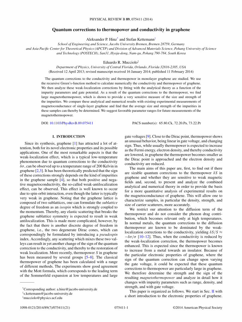
For impurities with larger correlation lengths (ξ > a0),NMC is observed for strong K0 and large EF , as seen inFig. 7(c). Surprisingly, there is a regime at weak K0 and smallEF where PMC occurs even for large ξ , see Fig. 7(d). Weobserved similar behavior for other sizes M and N, whichwe do not display here. In the EF − K0 diagram, we see achange from PMC to NMC when moving away from the Diracpoint. At the Dirac point, we observe a change at K0 ≈ 1.For EF > 0.05 t, only NMC is observed for ξ = 2a0. Theξ − EF phase diagram shows that for ξ a0, PMC occursindependent of the Fermi energy. At larger ξ , a change toNMC occurs, as expected.

In order to get a simpler representation of the results,we merge all three two-dimensional phase diagrams intoone three-dimensional phase diagram, in which each of theparameters ξ , K0, and EF is represented by one axis; seeFig. 8.

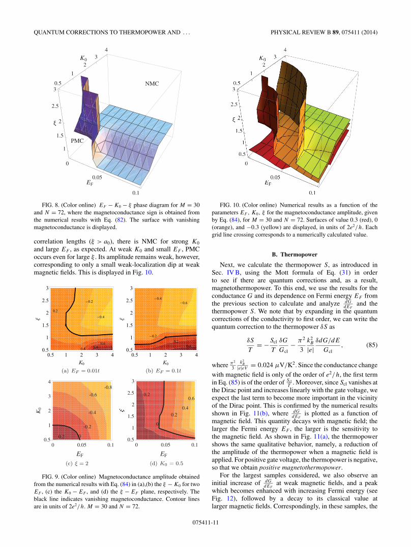
b. Magnetoconductance amplitude. Using Eq. (84), wedetermine the amplitude of the magnetoconductance and plotit in contour plots in the ξ − K0, the EF − K0, and theξ − EF plane, respectively, in Fig. 9. In these figures, thecontour lines are tagged with the corresponding numberscalculated from Eq. (84). The main features already observedin the magnetoconductance sign phase diagrams can be seenin Fig. 9: PMC occurs for short-range impurities with ξ a0, irrespective of K0 and EF . For impurities with larger

075411-10


FIG. 8. (Color online) EF − K0 − ξ phase diagram for M = 30and N = 72, where the magnetoconductance sign is obtained fromthe numerical results with Eq. (82). The surface with vanishingmagnetoconductance is displayed.

correlation lengths (ξ > a0), there is NMC for strong K0

and large EF , as expected. At weak K0 and small EF , PMCoccurs even for large ξ . Its amplitude remains weak, however,corresponding to only a small weak-localization dip at weakmagnetic fields. This is displayed in Fig. 10.

FIG. 9. (Color online) Magnetoconductance amplitude obtainedfrom the numerical results with Eq. (84) in (a),(b) the ξ − K0 for twoEF , (c) the K0 − EF , and (d) the ξ − EF plane, respectively. Theblack line indicates vanishing magnetoconductance. Contour linesare in units of 2e2/h. M = 30 and N = 72.

FIG. 10. (Color online) Numerical results as a function of theparameters EF , K0, ξ for the magnetoconductance amplitude, givenby Eq. (84), for M = 30 and N = 72. Surfaces of value 0.3 (red), 0(orange), and −0.3 (yellow) are displayed, in units of 2e2/h. Eachgrid line crossing corresponds to a numerically calculated value.

B. Thermopower

Next, we calculate the thermopower S, as introduced inSec. IV B, using the Mott formula of Eq. (31) in orderto see if there are quantum corrections and, as a result,magnetothermopower. To this end, we use the results for theconductance G and its dependence on Fermi energy EF fromthe previous section to calculate and analyze dG

dEFand the

thermopower S. We note that by expanding in the quantumcorrections of the conductivity to first order, we can write thequantum correction to the thermopower δS as

δS

T= −Scl

T

δG

Gcl− π2

3

k2B

|e|δdG/dE

Gcl, (85)

where π2

3k2B

|e|eV = 0.024 μV/K2. Since the conductance change

with magnetic field is only of the order of e2/h, the first termin Eq. (85) is of the order of Scl

T. Moreover, since Scl vanishes at

the Dirac point and increases linearly with the gate voltage, weexpect the last term to become more important in the vicinityof the Dirac point. This is confirmed by the numerical resultsshown in Fig. 11(b), where dG

dEFis plotted as a function of

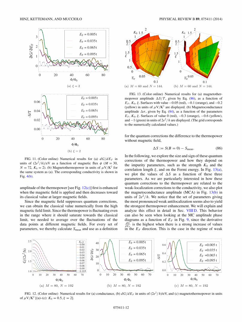
magnetic field. This quantity decays with magnetic field; thelarger the Fermi energy EF , the larger is the sensitivity tothe magnetic field. As shown in Fig. 11(a), the thermopowershows the same qualitative behavior, namely, a reduction ofthe amplitude of the thermopower when a magnetic field isapplied. For positive gate voltage, the thermopower is negative,so that we obtain positive magnetothermopower.

For the largest samples considered, we also observe aninitial increase of dG

dEFat weak magnetic fields, and a peak

which becomes enhanced with increasing Fermi energy (seeFig. 12), followed by a decay to its classical value atlarger magnetic fields. Correspondingly, in these samples, the

075411-11


FIG. 11. (Color online) Numerical results for (a) dG/dEF inunits of (2e2/h)/eV as a function of magnetic flux φ (M = 30,N = 72, K0 = 2). (b) Magnetothermopower in units of μV/K2 forthe same system as (a). The corresponding conductivity is shown inFig. 4(b).

amplitude of the thermopower [see Fig. 12(c)] first is enhancedwhen the magnetic field is applied and then decreases towardits classical value at larger magnetic fields.

Since the magnetic field suppresses quantum corrections,we can obtain the classical value numerically from the highmagnetic field limit. Since the thermopower is fluctuating evenin the range where it should saturate towards the classicallimit, we needed to average over the fluctuations of thedata points at different magnetic fields. For every set ofparameters, we thereby calculate Smean and use as a definition

FIG. 13. (Color online) Numerical results for (a) magnetother-mopower amplitude �S/T , given by Eq. (86), as a function ofEF , K0, ξ . Surfaces with value −0.05 (red), −0.1 (orange), and −0.2(yellow) in units of μV/K2 are displayed. (b) Magnetoconductanceamplitude �σ , given by Eq. (84), as a function of the parametersEF , K0, ξ . Surfaces of value 0 (red), −0.3 (orange), −0.6 (yellow),and −1 (green) in units of 2e2/h are displayed. (The grid correspondsto the numerically calculated values.)

for the quantum corrections the difference to the thermopowerwithout magnetic field,

�S := S(B = 0) − Smean. (86)

In the following, we explore the size and sign of these quantumcorrections of the thermopower and how they depend onthe impurity parameters, such as the strength K0 and thecorrelation length ξ , and on the Fermi energy. In Fig. 13(a),we plot the values of �S as a function of these threeparameters. As we are particularly interested in how thesequantum corrections to the thermopower are related to theweak-localization corrections to the conductivity, we also plotthe magnetoconductance amplitude (MCA) in Fig. 13(b) inunits of 2e2/h. We notice that the set of parameters givingthe most pronounced weak antilocalization seems also to yieldthe strongest thermopower enhancement. We will explain andanalyze this effect in detail in Sec. VIII D. This behaviorcan also be seen when looking at the MC amplitude phasediagrams as a function of EF in Fig. 9, since the derivativedGdEF

is the highest when there is a strong increase of valuesin the EF direction. This is the case in the regime of weak

FIG. 12. (Color online) Numerical results for (a) conductance, (b) dG/dEF in units of (2e2/h)/eV, and (c) magnetothermopower in unitsof μV/K2 [(a)–(c): K0 = 0.5, ξ = 2].

075411-12


antilocalization, while a smaller change is observable in theweak-localization regime; see Figs. 9(c) and 9(d).

VIII. ANALYSIS OF NUMERICAL RESULTS

In order to get a better understanding of these numericalresults for the magnetoconductance and the magnetother-mopower, we compare them with the analytical expressionof Eq. (25) and use the scattering rates 1/τz and 1/τi andthe effective dephasing rate 1/τφ as fitting parameters. Wealso attempt an ab initio calculation where we use the inputparameters of the numerical calculations to calculate directlythe different scattering rates 1/τij , insert these in the analyticalexpression, and compare the result with the numerical ones.

A. Fitting of the numerical results

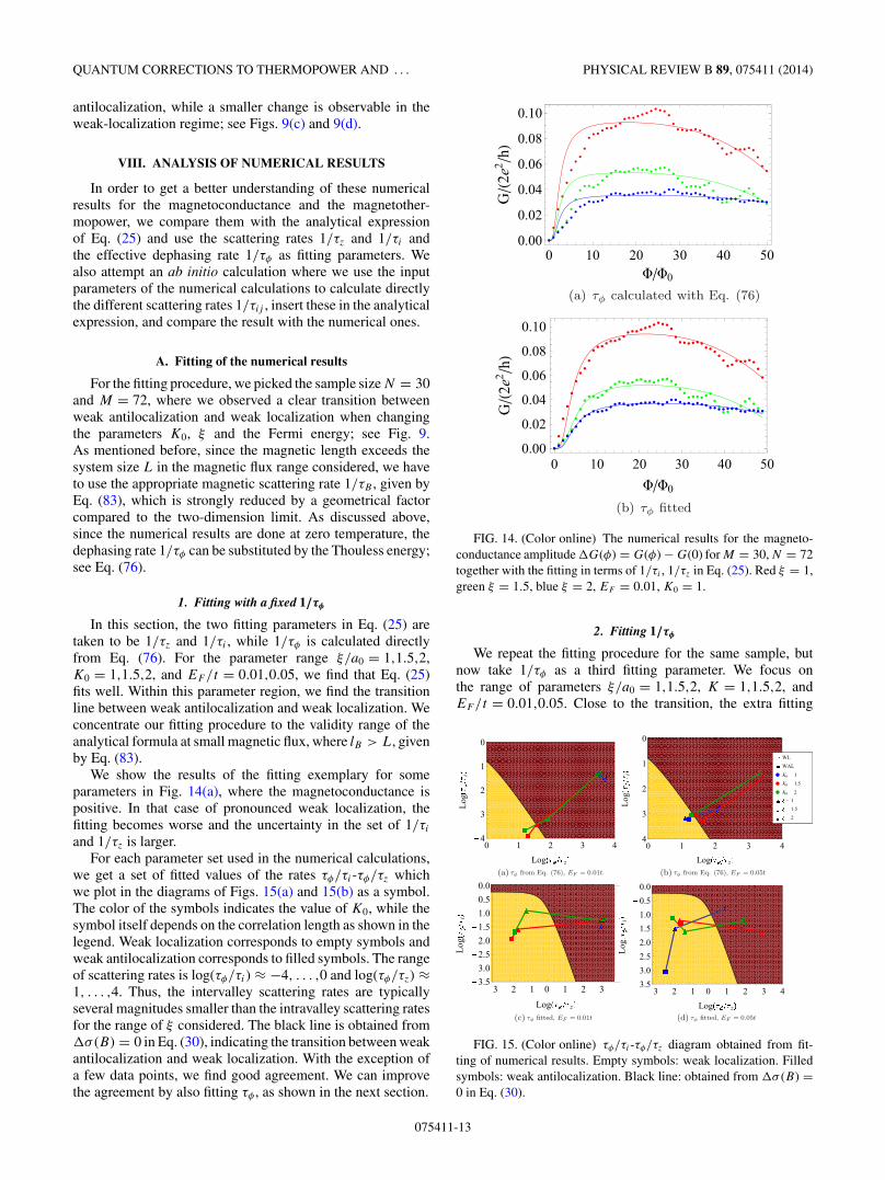
For the fitting procedure, we picked the sample size N = 30and M = 72, where we observed a clear transition betweenweak antilocalization and weak localization when changingthe parameters K0, ξ and the Fermi energy; see Fig. 9.As mentioned before, since the magnetic length exceeds thesystem size L in the magnetic flux range considered, we haveto use the appropriate magnetic scattering rate 1/τB , given byEq. (83), which is strongly reduced by a geometrical factorcompared to the two-dimension limit. As discussed above,since the numerical results are done at zero temperature, thedephasing rate 1/τφ can be substituted by the Thouless energy;see Eq. (76).

1. Fitting with a fixed 1/τφ

In this section, the two fitting parameters in Eq. (25) aretaken to be 1/τz and 1/τi , while 1/τφ is calculated directlyfrom Eq. (76). For the parameter range ξ/a0 = 1,1.5,2,K0 = 1,1.5,2, and EF /t = 0.01,0.05, we find that Eq. (25)fits well. Within this parameter region, we find the transitionline between weak antilocalization and weak localization. Weconcentrate our fitting procedure to the validity range of theanalytical formula at small magnetic flux, where lB > L, givenby Eq. (83).

We show the results of the fitting exemplary for someparameters in Fig. 14(a), where the magnetoconductance ispositive. In that case of pronounced weak localization, thefitting becomes worse and the uncertainty in the set of 1/τi

and 1/τz is larger.For each parameter set used in the numerical calculations,

we get a set of fitted values of the rates τφ/τi-τφ/τz whichwe plot in the diagrams of Figs. 15(a) and 15(b) as a symbol.The color of the symbols indicates the value of K0, while thesymbol itself depends on the correlation length as shown in thelegend. Weak localization corresponds to empty symbols andweak antilocalization corresponds to filled symbols. The rangeof scattering rates is log(τφ/τi) ≈ −4, . . . ,0 and log(τφ/τz) ≈1, . . . ,4. Thus, the intervalley scattering rates are typicallyseveral magnitudes smaller than the intravalley scattering ratesfor the range of ξ considered. The black line is obtained from�σ (B) = 0 in Eq. (30), indicating the transition between weakantilocalization and weak localization. With the exception ofa few data points, we find good agreement. We can improvethe agreement by also fitting τφ , as shown in the next section.

FIG. 14. (Color online) The numerical results for the magneto-conductance amplitude �G(φ) = G(φ) − G(0) for M = 30, N = 72together with the fitting in terms of 1/τi , 1/τz in Eq. (25). Red ξ = 1,green ξ = 1.5, blue ξ = 2, EF = 0.01, K0 = 1.

2. Fitting 1/τφ

We repeat the fitting procedure for the same sample, butnow take 1/τφ as a third fitting parameter. We focus onthe range of parameters ξ/a0 = 1,1.5,2, K = 1,1.5,2, andEF /t = 0.01,0.05. Close to the transition, the extra fitting

FIG. 15. (Color online) τφ/τi-τφ/τz diagram obtained from fit-ting of numerical results. Empty symbols: weak localization. Filledsymbols: weak antilocalization. Black line: obtained from �σ (B) =0 in Eq. (30).

075411-13


parameter does not change the result significantly. The resultof the fitting procedure for some parameter values is displayedin Fig. 14(b). As in Sec. VIII A 1, we display the resulting1/τi , 1/τz, and 1/τφ in a τφ/τi-τφ/τz diagram in Figs. 15(c)and 15(d).

We find that the results fall in the range log(τφ/τi) ≈−3, . . . ,0 and log(τφ/τz) ≈ −3, . . . ,3. The agreement withthe analytical results, i.e., the black solid line in Fig. 15, isimproved. All numerical results fall on the expected side ofthe weak-antilocalization to weak-localization transition line.

B. Ab initio calculation

In this section, we will attempt an ab initio calculation inthe sense that we use the input parameters of the numericalcalculations to calculate directly the different scattering rates1/τij , insert them into the analytical formula of Eq. (30) forthe weak-localization corrections, and compare the latter to thenumerical results. For this calculation, we choose the followingparameter ranges. The impurity width ξ is varied from 0.05a0

to 1.5a0 in steps of 0.05a0, the impurity strength V is variedfrom 0.5 eV to 5 eV in steps of 0.5 eV (corresponding to K0

between approximately 0.05 and 2) and EF from 0.01t to 0.1t

in steps of 0.01t (note that the analytical result is not valid tooclose to the Dirac point EF = 0). The impurity concentrationis set to 3% as before, if not explicitly mentioned otherwise.

1. Conductance

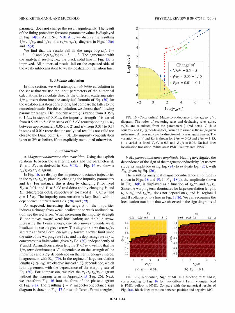
a. Magnetoconductance sign transition. Using the explicitrelations between the scattering rates and the parameters ξ ,V , and EF , as derived in Sec. VI B, in Fig. 16 we show aτφ/τi-τφ/τ∗ diagram.

In Fig. 16, we display the magnetoconductance trajectoriesin the τφ/τi-τφ/τ∗ plane by changing the impurity parametersand EF . For instance, this is done by changing ξ for fixedEF = 0.01t and V = 5 eV (red dots) and by changing V andEF (blue/green dots), respectively, for fixed ξ = 0.05 a0 andξ = 1.5 a0. The impurity concentration is kept fixed, with itsdependence inferred from Eqs. (78) and (79).

As expected, increasing the range ξ of the impuritiesinduces a change from weak localization to weak antilocaliza-tion; see the red arrow. When increasing the impurity strengthV , one moves toward weak localization; see the blue arrow.Increasing the Fermi energy, one also moves towards weaklocalization; see the green arrow. The diagram shows that τφ/τ∗saturates at fixed Fermi energy EF toward a lower limit sincethe ratio of the warping rate 1/τw and the dephasing rate τφ/τw

converges to a finite value, given by Eq. (80), independently ofV and ξ . At small correlation lengths (ξ a0), we find that the1/τz term dominates; a V 4 dependence on the strength of theimpurities and a EF dependence on the Fermi energy emerge,in agreement with Eq. (79). In the regime of large correlationlengths (ξ � a0), we observe instead a E4

F dependence, whichis in agreement with the dependence of the warping rate ofEq. (80). For comparison, we plot the τφ/τi-τφ/τz diagramwithout the warping term in Appendix B (Fig. 26). Next,we transform Fig. 16 into the form of the phase diagramof Fig. 7(a). The resulting ξ − V magnetoconductance signdiagram is shown in Fig. 17 for two different Fermi energies.

FIG. 16. (Color online) Magnetoconductance in the τφ/τi-τφ/τ∗diagram. The ratios of scattering rates and dephasing rates τφ/τi ,τφ/τ∗ are calculated from the parameters ξ (red dots), V (bluesquares), and EF (green triangles), which are varied in the range givenin the inset. Arrows indicate the direction of increasing parameter. Thevariation with V and EF is shown for ξ/a0 = 0.05 and ξ/a0 = 1.15;ξ is varied at fixed V/eV = 0.5 and EF /t = 0.04. Dashed line:localization transition. White area: PMC. Yellow area: NMC.

b. Magnetoconductance amplitude. Having investigated thedependence of the sign of the magnetoconductivity, let us nowstudy its amplitude using Eq. (84) to evaluate Eq. (25), withFfull given by Eq. (26).

The resulting analytical magnetoconductance amplitude isshown in Figs. 18 and 19. In Fig. 18(a), the amplitude shownin Fig. 18(b) is displayed as a function of τφ/τi and τφ/τ∗.Since the warping term dominates for large correlation lengths(ξ > a0) and τφ/τW does not depend on ξ and V , regions Iand II collapse onto a line in Fig. 18(b). We can recognize thelocalization transition that we observed in the sign diagrams of

FIG. 17. (Color online) Sign of MC as a function of V and ξ ,corresponding to Fig. 16 for two different Fermi energies. Redis PMC; yellow is NMC. Compare with the numerical results ofFig. 7(a). Black line: transition between positive and negative MC.

075411-14


FIG. 18. (Color online) (a) MC amplitude analytically calcu-lated, given by Eq. (84), in units of 2e2/h. Black line: transitionbetween PMC and NMC. Positive numbers and red color: weaklocalization. (b) MC amplitude as a function of τφ/τi and τφ/τ∗.

Fig. 17. In addition, we see that in the range of the localizationtransition obtained by the numerical calculation in Fig. 8, weobserve weak antilocalization with a small amplitude whenclose to the Dirac point for small back Fermi energies andfor weak scatterers (small V,K0). A small weak-localizationamplitude is suppressed already by a weak magnetic field.Thus, in the numerical calculations, it is difficult to identify aregion with a weak-localization amplitude. We typically find,by comparison, that the low-energy cutoff in the numericalcalculation is larger than the one obtained from the Thoulessenergy, given by Eq. (76).

C. Quantum correction to conductance at B = 0

The quantum correction to the conductance shown inEq. (23) is plotted in Fig. 20 as a function of impurity strengthV (and, correspondingly, K0) and the correlation length ξ . Wenote that the transition line between a positive and a negative

FIG. 19. (Color online) Analytically calculated magnetoconduc-tance amplitude, given by Eq. (84), as a function of ξ, V , and EF .Surfaces with value −1 (red), 0 (orange), and 1 (yellow) in units of2e2/h are displayed. Grid lines are guides to the eye.

quantum correction at B = 0, as indicated by the dashedline, does not coincide with the transition from negative topositive magnetoconductance, which is indicated by the thickblack line. Therefore, there is a region, denoted as II, wherethe quantum correction to the conductance is positive butthe conductance increases with magnetic field, as one wouldexpect for weak localization. Only in region I does the positivequantum correction coincide with the NMC expected for weakantilocalization. In region III, the negative quantum correctionsyields PMC, as expected for weak localization. These regionscan be related to the different types of magnetoconductancesketched in Fig. 6: applying a magnetic field in the region II,we expect a nonmonotonic magnetoconductance, where theconductance first increases, reaching a maximum at B = Bex,and then decays toward the classical conductance, as in case (2)of Fig. 6. In the other regions, I and III, the MC is monotonic,with PMC in region III and NMC in region I.

In Fig. 20(c), the result for the quantum correction shown inFig. 20(a) is displayed as a function of τφ/τi and τφ/τ∗. Sincethe warping term is dominant for large correlation lengthsξ > a0, and τφ/τW does not depend on ξ and V , the regions Iand II collapse onto a line in Fig. 20(c).

D. Quantum corrections to thermopower

In this section, we use the analytical theory to study thequantum corrections to the thermopower and the resultingmagnetic field dependence. In particular, we find out inwhich regime these corrections are large and whether, ingraphene, they are dominated by the quantum corrections tothe Fermi energy slope of the conductance rather than bythe weak-localization corrections to the conductance, as instandard metals.

1. Quantum corrections at zero magnetic field

We first consider the amplitude of the quantum correctionsto the thermopower as defined by Eq. (86), namely, as thedifference between the value at zero magnetic field andthe classical thermopower. Thus we need to use the weak-localization correction to the conductance at zero magneticfield, δσ (B = 0) [see Eqs. (23) and (25)], and insert it into theMott formula.

By inserting the dependence of the scattering rates on theFermi energy, as given by Eqs. (72)–(74) and (76), we obtainthe slope of the Fermi energy dependence of the conductanceat B = 0 as

∂δσ (B = 0)

∂EF

= e2

πh

1

EF

ϑ (ti ,tz,tw) , (87)

where

ϑ (ti ,tz,tw) = −2 + 2

1 + 2ti+ 4(1 − tw)

1 + ti + tz + tw, (88)

which depends on the parameter ratios ti = τφ/τi and tz =τφ/τz, as well as explicitly on the warping rate ratio tw =τφ/τw.

We note that while the quantum corrections to the con-ductivity are diverging, in the limit of 1/τφ → 0, whichcorresponds to low temperatures and large system sizes,the quantum corrections to the slope of the Fermi energy

075411-15


FIG. 20. (Color online) Analytically calculated quantum correction to the conductance at zero magnetic field, δσ (B = 0) in units of 2e2/h

for two different Fermi energies, (a) EF = 0.01t and (b) EF = 0.1t . Black dashed line: transition from positive to negative quantum correction,δσ (B = 0) = 0. Black line: Transition from PMC to NMC. (c) Same as (a), but displayed as a function of τφ/τi and τφ/τ∗.

dependence of the conductance, given by Eq. (87), converge toa finite value of order e2

πh1

EF, which depends on the scatterings

rates as follows:(1) When the warping term is negligible, tw ≈ 0, the

function ϑ converges to −2 for large ti , i.e., the weak-localization regime, as seen in Fig. 21(a). In the weak-antilocalization regime of small intervalley scattering (ti 1),ϑ turns positive.

(2) When the warping term dominates, and tz → 0, thefunction ϑ is negative and converges for large intervalleyscattering ti � 1, i.e., the weak-localization regime, to −6,as seen in Fig. 21(b). Remarkably, ϑ (and, thereby, dδσ/dEF )remains for tz → 0 negative for all values of ti , even in theregime of weak antilocalization.

In Fig. 22, ϑ is plotted as a function of ξ and V . For smallFermi energy, EF = 0.01t , ϑ is positive in the whole region ofweak antilocalization [corresponding to phase I in Figs. 20(a)and 20(b)]. This positive enhancement of ϑ [and thereforepositive quantum correction to the slope of the Fermi energydependence of the conductance at B = 0, given by Eq. (87)]matches well with the numerical results of Sec. VII B. Inthat regime, the intravalley scattering rate 1/τz is expectedto dominate over the warping rate, and the values of ϑ indeedagree with those obtained in Fig. 21(a) where tw = 0. At higher

FIG. 21. (Color online) The function ϑ , given by Eq. (88), (a) forτφ/τw = 0 and (b) for τφ/τz = 0. The continuous black line indicatesthe sign change of the function ϑ . Dashed line: transition betweenPMC and NMC.

Fermi energies, shown in Fig. 22(b), the warping rate becomesmore important, as tW ∼ E4

F increases faster than tz with EF .Indeed, ϑ remains negative for all values of ξ and V , inagreement with Fig. 21(b), where the intralayer scattering rateis set to zero, tz = 0. In the regime I of weak antilocalization,only a slight increase of ϑ is seen, while it remains negative.

Now we are in a position to consider the quantum correc-tions to the thermopower δS as given in Eq. (85). For smallFermi energies, these corrections are dominated by the secondterm in Eq. (85), resulting in the weak-antilocalization regime

(I) in a negative correction δS/T < 0 of order π2

3k2B

|e|eV =0.024 μV/K2. In the regime of weak localization, the quantumcorrection to the thermopower becomes positive. Since theclassical magnetoconductance increases with gate voltage, wefind that the first term in Eq. (85) becomes dominant at largeFermi energies, and one recovers δS/Scl ≈ −δG/Gcl, whichis characteristic of standard metals. To study the competitionbetween these two terms in more detail, we need an expressionfor the classical conductivity. In the strong scattering limit ofGaussian impurities and for Coulomb scatterers, one obtains a

FIG. 22. (Color online) ϑ , given by Eq. (88), for two differentFermi energies as a function of ξ and V . As in Figs. 20(a) and 20(b),the black dashed line indicates the transition from positive to negativequantum correction to the conductance, δσ (B = 0) = 0. Black line:transition from PMC to NMC.

075411-16


FIG. 23. (Color online) Analytically calculated δS/T obtainedfrom Eq. (90) in units of μV/K2 for two different Fermi energies.Black line: transition from PMC to NMC. Dashed line: δσ = 0. Whitearea: weak-localization correction to conductance exceeds classicalvalue.

quadratic dependence on Fermi energy [17],

σcl = 4e2

πh+ cξ

2e2E2F

hV 2, (89)

which is well justified in the limit of strong scatterers [13].The prefactor cξ is of the order of unity and increases fromshort-range to long-range scatterers by a factor of 2 [13]. Notethat we use here the notation introduced in Sec. VI, where V

is a measure of the total impurity strength averaged over allimpurities and increases with the density of impurities nimp asV ∼ √

nimp. We then obtain Scl by inserting Eq. (89) into theMott formula, given by Eq. (31). We obtain Scl by insertingEq. (89) into the Mott formula, given by Eq. (31). With Eq. (24)for δσ and Eq. (87) for ∂δσ/∂EF , we can use Eq. (85) to findthe dependence of δS/T on the impurity parameter and theFermi energy. We obtain

δS

T= π2k2

BV 2

3|e|(2V 2 + πE2F

) ( πEF

2V 2 + πE2F

θ − 1

2EF

ϑ

). (90)

This result is displayed in Fig. 23, where we set cξ = 1. Thewhite area corresponds to the regime where σDiff �σ (B =0), where Eq. (85) is no longer valid. [We note that, moregenerally, one needs to take into account that the classicalconductivity given by Eq. (89) depends also on the range ofimpurities, and for weak scatterers it may attain a weakerlogarithmic energy dependence [13]. This will change these

results quantitatively, but is not expected to change themqualitatively, which is why we choose Eq. (89) and leave theinclusion of a more consistent quantitative analysis for theclassical conductivity for future studies.]

Comparing the results with Fig. 22, we can see that the termdue to the quantum corrections to the Fermi energy slope ofthe conductance, i.e., the ϑ term in Eq. (90), is dominant in ourparameter range. The quantum corrections of the conductance,i.e., the θ term, play a minor role here. However, that termgains importance with higher Fermi energy. For small Fermienergy, the intravalley scattering 1/τz dominance is visiblein phase I weak antilocalization (WAL), where we detect anegative amplitude of the correction δS/T , while in phase IIand III, the correction is positive. For higher Fermi energy, thewarping term 1/τw is becoming dominant and we can observea positive correction for the complete phase I and II, and evena small correction for parts of phase III.

To see the connection between the electrical conductivitycorrection and the thermopower correction, we plot δσ

versus δS/T in Fig. 24. We focus on the range of weakantilocalization (phases I and II). For small Fermi energy,shown in Fig. 24(a), we can see the transition from positiveto negative thermopower correction δS when increasing theimpurity size ξ . We find negative δS < 0 in phase I, whilepositive δS > 0 is seen in phase II. An increase of the impuritystrength is moving the system toward positive δS > 0. Thisbehavior changes at higher Fermi energy [see Fig. 24(b)], sincethe warping term becomes more important. For short-rangeimpurities, the system in phase II does not show a clear relationbetween δσ and δS/T . An increase of the impurity strengthtends to lower the thermopower correction. With increasingimpurity range, when ξ ≈ a0, we observe an increase of thethermopower correction with an increase of the conductivitycorrection near the transition from NMC to PMC. For longer-ranged impurities, the system is in phase I of NMC. In thatregime, we find good agreement with the numerical resultsand observe a clear relation between an increase of δS/T andδσ . We note that the detailed parameter dependence may vary,depending on the value of the classical conductance σDiff andthe low-energy cutoff 1/τφ .

2. Magnetothermopower

Next, we consider how these quantum corrections changewhen applying a magnetic field. We focus first on the derivative

FIG. 24. (Color online) Analytically calculated δS/T -δσ diagram at zero magnetic field displaying the relation between the quantumcorrections to thermopower and conductivity corrections for the phases of WAL, I and II, for various impurity parameters ξ and V , for twodifferent Fermi energies. Dotted black lines: same impurity strength for different ξ .

075411-17


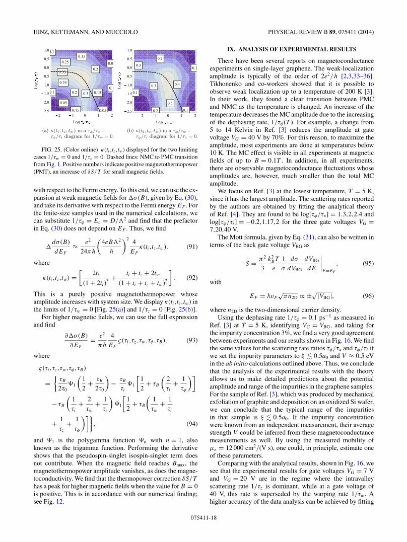
FIG. 25. (Color online) κ(ti ,tz,tw) displayed for the two limitingcases 1/τw = 0 and 1/τz = 0. Dashed lines: NMC to PMC transitionfrom Fig. 1. Positive numbers indicate positive magnetothermopower(PMT), an increase of δS/T for small magnetic fields.

with respect to the Fermi energy. To this end, we can use the ex-pansion at weak magnetic fields for �σ (B), given by Eq. (30),and take its derivative with respect to the Fermi energy EF . Forthe finite-size samples used in the numerical calculations, wecan substitute 1/τφ = Ec = D/2 and find that the prefactorin Eq. (30) does not depend on EF . Thus, we find

�dσ (B)

dEF

≈ e2

24πh

(4eB2

�

)24

EF

κ(ti ,tz,tw), (91)

where

κ(ti ,tz,tw) =[

2ti

(1 + 2ti)3 + ti + tz + 2tw

(1 + ti + tz + tw)2

]. (92)

This is a purely positive magnetothermopower whoseamplitude increases with system size. We display κ(ti ,tz,tw) inthe limits of 1/τw = 0 [Fig. 25(a)] and 1/τz = 0 [Fig. 25(b)].

For higher magnetic fields, we can use the full expressionand find

∂�σ (B)

∂EF

= e2

πh

4

EF

ς (τi,τz,τw,τφ,τB), (93)

where

ς (τi,τz,τw,τφ,τB)

={

τB

2τ0�1

(1

2+ τB

2τ0

)− τB

τi

�1

[1

2+ τB

(2

τi

+ 1

τφ

)]

− τB

(1

τi

+ 2

τw

+ 1

τz

)�1

[1

2+ τB

(1

τw

+ 1

τi

+ 1

τz

+ 1

τφ

)]}, (94)

and �1 is the polygamma function �n with n = 1, alsoknown as the trigamma function. Performing the derivativeshows that the pseudospin-singlet isospin-singlet term doesnot contribute. When the magnetic field reaches Bmax, themagnetothermopower amplitude vanishes, as does the magne-toconductivity. We find that the thermopower correction δS/T

has a peak for higher magnetic fields when the value for B = 0is positive. This is in accordance with our numerical finding;see Fig. 12.

IX. ANALYSIS OF EXPERIMENTAL RESULTS

There have been several reports on magnetoconductanceexperiments on single-layer graphene. The weak-localizationamplitude is typically of the order of 2e2/h [2,3,33–36].Tikhonenko and co-workers showed that it is possible toobserve weak localization up to a temperature of 200 K [3].In their work, they found a clear transition between PMCand NMC as the temperature is changed. An increase of thetemperature decreases the MC amplitude due to the increasingof the dephasing rate, 1/τφ(T ). For example, a change from5 to 14 Kelvin in Ref. [3] reduces the amplitude at gatevoltage VG = 40 V by 70%. For this reason, to maximize theamplitude, most experiments are done at temperatures below10 K. The MC effect is visible in all experiments at magneticfields of up to B = 0.1T . In addition, in all experiments,there are observable magnetoconductance fluctuations whoseamplitudes are, however, much smaller than the total MCamplitude.

We focus on Ref. [3] at the lowest temperature, T = 5 K,since it has the largest amplitude. The scattering rates reportedby the authors are obtained by fitting the analytical theoryof Ref. [4]. They are found to be log[τφ/τ∗] = 1.3,2,2.4 andlog[τφ/τi] = −0.2,1.17,2 for the three gate voltages VG =7,20,40 V.

The Mott formula, given by Eq. (31), can also be written interms of the back gate voltage VBG as

S = π2

3

k2BT

e

1

σ

dσ

dVBG

dVBG

dE

∣∣∣∣E=EF

, (95)

with

EF = �vF

√πn2D ∝ ±

√|VBG|, (96)

where n2D is the two-dimensional carrier density.Using the dephasing rate 1/τφ = 0.1 ps−1 as measured in

Ref. [3] at T = 5 K, identifying VG = VBG, and taking forthe impurity concentration 3%, we find a very good agreementbetween experiments and our results shown in Fig. 16. We findthe same values for the scattering rate ratios τφ/τ∗ and τφ/τi ifwe set the impurity parameters to ξ � 0.5a0 and V ≈ 0.5 eVin the ab initio calculations outlined above. Thus, we concludethat the analysis of the experimental results with the theoryallows us to make detailed predictions about the potentialamplitude and range of the impurities in the graphene samples.For the sample of Ref. [3], which was produced by mechanicalexfoliation of graphite and deposition on an oxidized Si wafer,we can conclude that the typical range of the impuritiesin that sample is ξ � 0.5a0. If the impurity concentrationwere known from an independent measurement, their averagestrength V could be inferred from these magnetoconductancemeasurements as well. By using the measured mobility ofμe = 12 000 cm2/(V s), one could, in principle, estimate oneof these parameters.

Comparing with the analytical results, shown in Fig. 16, wesee that the experimental results for gate voltages VG = 7 Vand VG = 20 V are in the regime where the intravalleyscattering rate 1/τz is dominant, while at a gate voltage of40 V, this rate is superseded by the warping rate 1/τw. Ahigher accuracy of the data analysis can be achieved by fitting

075411-18


the experimental data at different gate voltages to the sameparameters and making use of the analytical gate voltagedependence of τφ/τi and τφ/τ∗, as in Eq. (80).

There have been several reports on the measurements ofthermopower in single-layer graphene [5–8]. We found abovethat the magnitude of the quantum corrections to thermopoweris of the order of 1 μV/T 2 [see Figs. 13(a) and 24], which isnot much smaller than the measured values for the classicalthermopower of single-layer graphene [6–8]. We note that thedependence of δσ on EF strongly depends on the Fermi energydependence of the dephasing rate 1/τφ . At low temperatures,the dephasing is dominated by the electron-electron scattering,yielding [37]

1

τφ

= αkBT

2EF τ0ln(2EF τ0/�). (97)

Since 1/τ0 ∼ EF , given by Eq. (74), close to the Dirac point,one finds that τφ is independent of the Fermi energy EF , ingood agreement with the experimental results [3].

High magnetic field thermopower measurements at roomtemperature have been performed [38] and a theory based onthe self-consistent Born approximation (SCBA) has been givenin Ref. [39]. The temperature scale of these experiments rangesfrom room temperature down to several Kelvin, which wouldalso be the right temperature range to observe the magnetother-mopower due to quantum corrections studied here. To this end,the thermopower measurements would have to be performedat magnetic fields below Bmax ∼ 0.1 Tesla. We are not awarethat such measurements have been performed to date.

As mentioned before, the weak-localization correctionsto the conductance and thermopower become suppressedwhen the magnetic length lB is on the order of the elasticmean free path le = vτ or when 1/τ ∼ v/lB , which definesthe maximal magnetic field Bmax at which weak-localizationcorrections can be expected. The spacing between theLandau levels in graphene is known to be anomalously large,�ωc = √

2v/lB . The condition where Landau levels becomesmeared out by disorder yields, therefore, 1/τ ∼ v/lB ,and in the weak-localization regime, B < Bmax effects ofLandau bands can indeed be disregarded. For B > Bmax, themagnetoconductance is classical, but can also be sensitive tothe range of impurities and acquire a

√B dependence [40,41].

Thus, the magnetothermopower accordingly can be expectedto become stronger than previously known [39].

There is increasing evidence that adatoms and vacancies areimportant to understand the transport properties of graphene.The transport theory of graphene with such strong impuritiesforming resonances has recently been studied in Ref. [42],where it was found that there is a regime close to the Diracpoint where the transport differs from the predictions basedon the transport theory with nonresonant impurities used here.It will therefore be important to study the thermopower in thepresence of such impurities. However, Ref. [42] confirms thatthere is a regime away from the Dirac point where the effectof strong impurities can be described by the model used here.

X. CONCLUSIONS AND DISCUSSION

We have studied the quantum corrections to the conductivityand the thermopower in monolayer graphene by analyzing

numerical results in conjunction with the analytical theory.The quantum corrections to the thermopower result in largemagnetothermopower, which we demonstrate to be a verysensitive measure of the impurities in graphene. While thereare experimental measurements of magnetoconductance ofsingle-layer graphene which could be used to determinethe average range and strength of the impurities, futuremeasurements of the magnetothermopower could provideadditional information about the graphene samples. The strongmagnetic field dependence of the thermopower, i.e., themagnetothermopower, is a direct measure of the quantumcorrections to the thermopower. In contrast to usual metals, itsamplitude in graphene is not simply related to the amplitude ofthe electrical conductivity, but is also governed by the quantumcorrection to the gate voltage slope of the conductivity.

We demonstrate that the numerical calculations not onlycan be fitted with the analytical theory, but we even find goodagreement when the scattering rates entering the analyticaltheory are calculated directly from the numerical inputparameters. This allows a more detailed understanding, sincethe dependence on gate voltage and other variable parameterscan be studied, revealing more accurate information on theimpurity parameters in graphene.

Besides the sign of the magnetoconductance, showing atransition between PMC and NMC, we also analyzed the am-plitude of the quantum corrections. We found that the transitionfrom PMC to NMC does not coincide with the transitionfrom positive to negative quantum corrections at vanishingmagnetic field B = 0. We analyzed the relation between theamplitude of the quantum corrections to the conductance andthe magnetothermopower. It appeared strongest close to theDirac point and for long-range impurities.

Here, we studied the thermopower using the Mott formula,which is only valid for small ratios T/EF . Still, experimentsshow that it remains valid close to the Dirac point [5,9]. We in-tend to study its validity in the future by using directly the Kuboformula for the thermopower. For the aspect ratio 1 studied inthis paper, we did not find a strong sensitivity to the form of theboundary conditions, i.e., armchair or zigzag. The quantumcorrections are expected to increase for larger aspect ratios.Also the warping rate 1/τw is expected to be sensitive to theaspect ratio, being suppressed when the width of the graphenesamples is reduced. This effect is similar to the reduction ofthe Dyakonov-Perel spin scattering rate in quantum wires [43].The other rates 1/τi and τz are expected to depend only weaklyon the aspect ratio. We note that we assumed in this paperthat the dominant impurity scattering processes are elastic.The effect of magnetic scatterers on the weak-localizationcorrections in graphene will be studied in a separate work.

ACKNOWLEDGMENTS

The authors would like to thank Hyunyong Lee, Paul Wenk,Vincent Sacksteder, Seung-Geol Nam, and Prof. Hu Jong Leefor useful discussions. We gratefully acknowledge that thisresearch was supported by the World Class University (WCU)program, Division of Advanced Materials Science as well asthe Asian Pacific Center of Theoretical Physics (APCTP) atPOSTECH university. We also thank the Jacobs UniversityFoundation for supporting this research.

075411-19


APPENDIX A: MATRIX NOTATION OF THE HAMILTONIAN

For a better understanding of the structure of our formulation, it useful to write the Hamiltonian in matrix notation. We presenthere H1, H2, and Himp in this way. In particular, the Himp matrix makes it easier to see the connection of each part of the impuritypotential to the isospin-pseudospin description and the matrix notation of the Gaussian potential which is shown in Sec. VI. Wehave

H1 = vF ζ3 ⊗ �σ · �k (A1)

= vF

⎛⎜⎝

0 kx − iky 0 0kx + iky 0 0 0

0 0 0 kx + iky

0 0 kx − iky 0

⎞⎟⎠, (A2)

and

H2 = μ[σ1(k2x − k2

y

)− 2σ2(kxky)]

(A3)

= μ

⎛⎜⎜⎜⎝

0 (kx + iky)2 0 0

(kx − iky)2 0 0 0

0 0 0 (kx + iky)2

0 0 (kx − iky)2 0

⎞⎟⎟⎟⎠ . (A4)

The second term of the impurity Hamiltonian, as given in Eq. (11), can be rewritten in matrix form as⎛⎜⎜⎜⎝

V3,3 V1,3 − iV2,3 V3,1 − iV3,2 −V1,1 + iV1,2 + iV2,1 + V2,2

V1,3 + iV2,3 −V3,3 V1,1 − iV1,2 + iV2,1 + V2,2 V3,1 − iV3,2

V3,1 + iV3,1 V1,1 + iV1,2 − iV2,1 + V2,2 −V3,3 V1,3 − iV2,3

−V1,1 − iV1,2 − iV2,1 + V2,2 V3,1 + iV3,1 V1,3 + iV2,3 V3,3

⎞⎟⎟⎟⎠ .

(A5)

APPENDIX B: MAGNETOCONDUCTANCE FOR 1/τw → 0

In Fig. 26, we present the results of the ab initio calculations for the MC as a function of τφ/τi and τφ/τz.

FIG. 26. (Color online) Magnetoconductance in the τφ/τi-τφ/τz diagram for 1/τw = 0. The ratios of scattering rates and dephasing ratesτφ/τi , τφ/τz are calculated from the parameters ξ (red dots), V (blue squares), and EF (green triangles), which are varied in the range givenin the inset. Arrows indicate the direction of increasing parameter. The variation with V and EF is shown for ξ/a0 = .05; ξ is varied at fixedV/eV = 0.5 and EF /t = .04. Dashed line: localization transition. White area: PMC. Yellow area: NMC.

075411-20


[1] K. S. Novoselov, A. K. Geim, S. V. Morozov, D. Jiang, Y. Zhang,S. V. Dubonos, I. V. Grigorieva, and A. A. Firsov, Science 306,666 (2004).

[2] D.-K. Ki, D. Jeong, J.-H. Choi, H.-J. Lee, and K.-S. Park, Phys.Rev. B 78, 125409 (2008).

[3] F. V. Tikhonenko, A. A. Kozikov, A. K. Savchenko, and R. V.Gorbachev, Phys. Rev. Lett. 103, 226801 (2009).

[4] E. McCann, K. Kechedzhi, V. I. Fal’ko, H. Suzuura, T. Ando,and B. L. Altshuler, Phys. Rev. Lett. 97, 146805 (2006).

[5] S.-G. Nam, D.-K. Ki, and H.-J. Lee, Phys. Rev. B 82, 245416(2010).

[6] J. G. Checkelsky and N. P. Ong, Phys. Rev. B 80, 081413(2009).

[7] Y. M. Zuev, W. Chang, and P. Kim, Phys. Rev. Lett. 102, 096807(2009).

[8] P. Wei, W. Bao, Y. Pu, C. N. Lau, and J. Shi, Phys. Rev. Lett.102, 166808 (2009).

[9] T. Lofwander and M. Fogelstrom, Phys. Rev. B 76, 193401(2007).

[10] V. V. Afonin, Y. M. Gal’perin and V. L. Gurevich, Zh. Eksp.Teor. Fiz 87, 335 (1984) [Sov. Phys. JETP 60, 194 (1984)].

[11] V. V. Afonin, Y. M. Gal’perin, and V. L. Gurevich, Phys. Rev. B33, 8841 (1986).

[12] M. J. Kearney and P. N. Butcher, J. Phys. C 21, L265 (1988).[13] P. M. Ostrovsky, I. V. Gornyi, and A. D. Mirlin, Phys. Rev. B

74, 235443 (2006).[14] I. L. Aleiner and K. B. Efetov, Phys. Rev. Lett. 97, 236801

(2006).[15] S. Guruswamy, A. LeClair, and A. W. W. Ludwig, Nucl. Phys.

B 583, 475 (2000).[16] D. V. Khveshchenko, Phys. Rev. Lett. 97, 036802 (2006).[17] A. H. Castro Neto, F. Guinea, N. M. R. Peres, K. S. Novoselov,

and A. K. Geim, Rev. Mod. Phys. 81, 109 (2009).[18] T. Ando, T. Nakanishi, and R. Saito, J. Phys. Soc. Jpn. 67, 2857

(1998).[19] V. I. Falko, K. Kechedzhi, E. McCann, B. Altshuler, H. Suzuura,

and T. Ando, Solid State Commun. 143, 33 (2007).[20] P. A. Lee and D. S. Fisher, Phys. Rev. Lett. 47, 882 (1981).[21] R. A. Jalabert, H. U. Baranger, and A. D. Stone, Phys. Rev. Lett.

65, 2442 (1990).

[22] E. R. Mucciolo and C. H. Lewenkopf, J. Phys.: Condens. Matter22, 273201 (2010).

[23] E. R. Mucciolo, A. H. Castro Neto, and C. H. Lewenkopf, Phys.Rev. B 79, 075407 (2009).

[24] C. H. Lewenkopf, E. R. Mucciolo, and A. H. Castro Neto, Phys.Rev. B 77, 081410 (2008).

[25] C. Lewenkopf and E. Mucciolo, J. Comput. Electron. 12, 203(2013).

[26] H. Schomerus, Phys. Rev. B 76, 045433 (2007).[27] D. Ferry and S. Goodnick, Transport in Nanostructures, Cam-

bridge Studies in Semiconductor Physics and MicroelectronicEngineering (Cambridge University Press, Cambridge, UK,1997).

[28] A. Rycerz, J. Tworzydlo, and C. W. J. Beenakker, Europhys.Lett. 79, 57003 (2007).

[29] T. Ando, J. Phys. Soc. Jpn. 74, 777 (2005).[30] J. T. Edwards and D. J. Thouless, J. Phys. C 5, 807 (1972).[31] P. A. Lee and T. V. Ramakrishnan, Rev. Mod. Phys. 57, 287

(1985).[32] I. L. Aleiner and V. I. Fal’ko, Phys. Rev. Lett. 87, 256801 (2001).[33] J. Eroms and D. Weiss, New J. Phys. 11, 095021 (2009).[34] X. Wu, X. Li, Z. Song, C. Berger, and W. A. de Heer, Phys. Rev.

Lett. 98, 136801 (2007).[35] F. V. Tikhonenko, D. W. Horsell, R. V. Gorbachev, and A. K.

Savchenko, Phys. Rev. Lett. 100, 056802 (2008).[36] D. Horsell, F. Tikhonenko, R. Gorbachev, and A. Savchenko,

Phil. Trans. R. Soc. A 366, 245 (2008).[37] B. L. Altshuler, A. G. Aronov, and D. E. Khmelnitsky, J. Phys.

C 15, 7367 (1982).[38] X. Liu, D. Wang, P. Wei, L. Zhu, and J. Shi, Phys. Rev. B 86,

155414 (2012).[39] B. Dora and P. Thalmeier, Phys. Rev. B 76, 035402 (2007).[40] P. S. Alekseev, A. P. Dmitriev, I. V. Gornyi, and V. Yu.

Kachorovskii, Phys. Rev. B 87, 165432 (2013).[41] G. Vasileva, P. Alekseev, Y. Ivanov, Y. Vasilev, D. Smirnov,

H. Schmidt, R. Haug, F. Gouider, and G. Nachtwei, JETP Lett.96, 471 (2012).

[42] G. Trambly de Laissardiere and D. Mayou, Phys. Rev. Lett. 111,146601 (2013).

[43] S. Kettemann, Phys. Rev. Lett. 98, 176808 (2007).

075411-21

http://dx.doi.org/10.1126/science.1102896








http://dx.doi.org/10.1103/PhysRevLett.103.226801
































http://dx.doi.org/10.1088/0022-3719/21/9/004

http://dx.doi.org/10.1088/0022-3719/21/9/004

http://dx.doi.org/10.1088/0022-3719/21/9/004

http://dx.doi.org/10.1088/0022-3719/21/9/004









http://dx.doi.org/10.1016/S0550-3213(00)00245-5

http://dx.doi.org/10.1016/S0550-3213(00)00245-5

http://dx.doi.org/10.1016/S0550-3213(00)00245-5

http://dx.doi.org/10.1016/S0550-3213(00)00245-5





http://dx.doi.org/10.1103/RevModPhys.81.109




http://dx.doi.org/10.1143/JPSJ.67.2857




http://dx.doi.org/10.1016/j.ssc.2007.03.049












http://dx.doi.org/10.1088/0953-8984/22/27/273201

http://dx.doi.org/10.1088/0953-8984/22/27/273201

http://dx.doi.org/10.1088/0953-8984/22/27/273201

http://dx.doi.org/10.1088/0953-8984/22/27/273201









http://dx.doi.org/10.1007/s10825-013-0458-7

http://dx.doi.org/10.1007/s10825-013-0458-7

http://dx.doi.org/10.1007/s10825-013-0458-7

http://dx.doi.org/10.1007/s10825-013-0458-7





http://dx.doi.org/10.1209/0295-5075/79/57003

http://dx.doi.org/10.1209/0295-5075/79/57003

http://dx.doi.org/10.1209/0295-5075/79/57003

http://dx.doi.org/10.1209/0295-5075/79/57003





http://dx.doi.org/10.1088/0022-3719/5/8/007

http://dx.doi.org/10.1088/0022-3719/5/8/007

http://dx.doi.org/10.1088/0022-3719/5/8/007

http://dx.doi.org/10.1088/0022-3719/5/8/007









http://dx.doi.org/10.1088/1367-2630/11/9/095021

http://dx.doi.org/10.1088/1367-2630/11/9/095021

http://dx.doi.org/10.1088/1367-2630/11/9/095021

http://dx.doi.org/10.1088/1367-2630/11/9/095021









http://dx.doi.org/10.1098/rsta.2007.2159




http://dx.doi.org/10.1088/0022-3719/15/36/018

http://dx.doi.org/10.1088/0022-3719/15/36/018

http://dx.doi.org/10.1088/0022-3719/15/36/018

http://dx.doi.org/10.1088/0022-3719/15/36/018













http://dx.doi.org/10.1134/S0021364012190137

http://dx.doi.org/10.1134/S0021364012190137

http://dx.doi.org/10.1134/S0021364012190137

http://dx.doi.org/10.1134/S0021364012190137









quantum corrections to thermopower and conductivity in graphene

Documents